THE DISTRIBUTIONAL IMPACT OF FISCAL POLICY IN … · THE DISTRIBUTIONAL IMPACT OF FISCAL POLICY IN INDONESIA* Jon Jellema, Matthew Wai-Poi, and Rythia Afkar† CEQ Working Paper 40

1

THE DISTRIBUTIONAL IMPACT OF FISCAL POLICY IN INDONESIA

Jon Jellema, Matthew Wai-Poi and Rythia Afkar

Working Paper 40 May 2017

The CEQ Working Paper Series

The CEQ Institute at Tulane University works to reduce inequality and poverty through rigorous tax and benefit incidence analysis and active engagement with the policy community. The studies published in the CEQ Working Paper series are pre-publication versions of peer-reviewed or scholarly articles, book chapters, and reports produced by the Institute. The papers mainly include empirical studies based on the CEQ methodology and theoretical analysis of the impact of fiscal policy on poverty and inequality. The content of the papers published in this series is entirely the responsibility of the author or authors. Although all the results of empirical studies are reviewed according to the protocol of quality control established by the CEQ Institute, the papers are not subject to a formal arbitration process. The CEQ Working Paper series is possible thanks to the generous support of the Bill & Melinda Gates Foundation. For more information, visit www.commitmentoequity.org.

The CEQ logo is a stylized graphical representation of a Lorenz curve for a fairly unequal distribution of income (the bottom part of the C, below the diagonal) and a concentration curve for a very progressive transfer (the top part of the C).

THE DISTRIBUTIONAL IMPACT OF FISCAL POLICY IN INDONESIA*

Jon Jellema, Matthew Wai-Poi, and Rythia Afkar†

CEQ Working Paper 40

MAY 2017

ABSTRACT

In recent years, income inequality has become a pressing issue in Indonesian politics. From 2000-2014, a rise in GDP per capita coincided with a 10% rise in the country’s Gini coefficient. This paper uses the 2012 National Socioeconomic Survey (SUSENAS) collected by the Central Statistical Agency in Indonesia and 2012 public expenditure and revenue data from the Audit Board of the Republic of Indonesia (BPK), to generate an empirical framework that assesses the redistributive impact of several fiscal measures undertaken by the Indonesian government. This paper finds that every income decile represented in SUSENAS is a net receiver from fiscal policy after taxes, transfers, in-kind transfers and subsidies are all added to “market income” to create “final income.” Gains amongst the poorest household are made much greater by the inclusion of in-kind transfers for health and education. However, SUSENAS included very few of the richest 0.5% of Indonesians, who account for the majority of personal income tax (PIT) collections, so it was assumed that Indonesians do not pay income tax. Interestingly, this study finds that 40% of the poor, measured at “consumable income,” are impoverished by taxes and transfers. This percentage drops considerably with the addition of in-kind transfers. Overall, it was found that fiscal policy does reduce inequality and poverty by a modest amount. The Gini index is lowered from 0.394 to 0.370 under the study’s baseline scenario, which differs only slightly from scenarios utilizing different underlying assumptions. The poverty headcount (measured at $1.25 UDS per day) is reduced from 12.1% to 10.5%.

Keywords: fiscal incidence, taxation, social spending, inequality, poverty, Indonesia JEL Codes: H22, D31, I38

* This paper was published as a chapter of The Distributional Impact of Fiscal Policy: Evidence from Developing Countries, edited by Gabriela Inchauste and Nora Lustig, World Bank, 2017. This study has been produced by the Commitment to Equity (CEQ) Institute and possible thanks to the generous support from the Bill & Melinda Gates Foundation. Launched in 2008, the CEQ project is an initiative of the Center for Inter-American Policy and Research (CIPR) and the department of Economics, Tulane University, the Center for Global Development and the Inter-American Dialogue. The CEQ project is housed in the Commitment to Equity Institute at Tulane. For more details visit www.commitmentoequity.org. † Jon Jellema is Associate Director for Africa, Asia and Europe at the CEQ Institute; Matthew Wai-Poi is Senior Economics at the World Bank in Jakarta; Rythia Afkar is an Economist at the World Bank.

4

1. Introduction

Fifteen years of sustained income growth helped Indonesia cut its poverty rate by more than half since the beginning of the new millennium: it stood at just over 11 percent of the population in 2014, down from 24 percent during the 1997–98 Asian Financial Crisis (World Bank 2016). 1 However, the benefits from expanding, more efficient macroeconomic conditions have been shared disproportionately: between 2003 and 2010, real per capita consumption of the richest 10 percent of Indonesians grew by over 6 percent per year, but consumption of the poorest two-fifths of the population grew by less than 2 percent per year (World Bank 2016). This disparity explains a recent uptick in inequality in Indonesia: the Gini coefficient increased by approximately 10 percentage points, from approximately 0.30 in 2000 to 0.41 in 2014.2 Worsening inequality has alarmed the public and politicians alike: nearly 90 percent of Indonesians recently said it was “urgent” that the government address inequality. The executive administration implemented significant fuel subsidy reforms in late 2014 and early 2015 and reallocated expenditures to programs that reduce inequality and foster balanced economic growth (World Bank 2016). To illuminate the impact of fiscal policies and public programs on poverty and inequality in Indonesia, we catalogue the distributional welfare consequences of Indonesia’s public revenues and expenditures, quantify the impact of these fiscal activities on both inequality and poverty, and estimate how effectively they redistribute income between the rich and the poor. We generate these estimates using the Commitment to Equity (CEQ) analytical methodology as described in the CEQ Handbook (Lustig and Higgins 2013; Lustig, 2018) as well as in Inchauste and Lustig (2017). The CEQ project uses standard fiscal incidence analysis to allocate to the representative individuals in a national household survey both the burdens of household-based revenue collection instruments (direct and indirect taxes) and the benefits from direct, indirect, and in-

1 The poverty rate is defined as the percentage of population living below the national poverty line of Rp 302,735 (US$25) per person per month (in 2014). Real gross domestic product (GDP) per capita grew by 5.4 percent annually (on average) between 2000 and 2014. This growth has also helped create a larger consumer class than ever before: 45 million people—approximately 18 percent of all Indonesians—are now “economically secure,” defined as middle-class households that are economically secure from poverty and vulnerability; the economic security line in 2014 was about Rp 1 million (US$83) in consumption per person per month (World Bank 2016). 2 The Gini index is measured in Indonesia in terms of the distribution of per capita consumption rather than distribution of per capita income. See World Bank (2016) for an extended discussion.

5

kind transfers financed by public expenditures.3 The magnitude of total burdens and benefits are taken directly from budget figures and administrative data, and their distribution among individuals in the household survey is informed by program rules, policy statements, and relevant regulations. Verified, cumulative expenditure and revenue figures and the micro-level distribution of individuals are equally important empirical keystones in the CEQ method. This creates an opportunity for straightforward international comparison and the incorporation of differing income levels, spending priorities, and socioeconomic composition via a common empirical methodology. Indonesia-based researchers have traced the distributional consequences of a generalized fiscal process as well as some individual fiscal policy elements. For example, Damuri and Perdana (2003) apply a computable general equilibrium (CGE) model to estimate the impact of general fiscal expansion on poverty and welfare across the entire income distribution; their results indicate that urban households and nonagricultural rural households benefit the most from expansionary fiscal policy. Hadiwibowo (2010) suggests that “development expenditures” specifically increase investment and accelerate economic growth, with positive domino effects on poverty. Dartanto (2013) examines the impact of Indonesian energy subsidies (also through a CGE model) and finds that reducing the then-current fuel subsidy by 25 percent would have contributed to an increase in the headcount poverty rate by just less than one quarter of a percentage point, while foregone subsidy expenditures would have—had they been reallocated as general government expenditures—reduced poverty incidence by just over one quarter of a percentage point. This report builds on previous findings by empirically generating a greater range of fiscal policy impacts on poverty and inequality, both overall and from individual revenue and expenditure components. Nationally representative macro datasets and micro datasets are used in one empirical analytical framework to estimate and describe the contribution of the main components of fiscal policy to the reduction of both poverty and inequality. The analysis covers about 44 percent of total tax revenues and 56 percent of primary government expenditures. It also includes the user fees collected directly from individuals using public health and education services as well as the indirect impacts of energy subsidies and consumption-based indirect taxes on household welfare. In other words, the analysis summarized here provides more details on the impact of each fiscal policy element while preserving generality and the ability to aggregate those impacts to describe fiscal policy generally—in so doing, accommodating a greater empirical range of sources of potential welfare impacts. 3 For the Indonesia CEQ assessment, we use household survey data from the 2012 National Socioeconomic Survey (SUSENAS) conducted by the Central Statistics Agency (http://microdata.bps.go.id/mikrodata/index.php/catalog/SUSENAS). Public expenditure and revenue magnitude data come from fiscal year 2012 audited budget and administrative data (BPK 2013).

6

Our findings indicate that despite a relatively low social spending base and relatively little revenue collection from direct income taxation, Indonesia’s fiscal policy does reduce both inequality and poverty. However, those fiscal policy impacts are modest: poverty or inequality statistics measured after the application of fiscal policy are only slightly reduced from those measured on the basis of pre-fiscal-policy incomes. If we look at “consumable” transfers only,4 nearly two-fifths of individuals who are poor at the level of “consumable income”5 have paid more in taxes than they have received in transfers: in other words, nearly 40 percent of the consumable-income poor have been impoverished by fiscal policy in Indonesia.6 A second striking result is that although local, unregulated user fees for publicly delivered health and education services are a significant cost for most users regardless of income level, in practice the burden of such fees is distributed to slightly reduce inequality.7 In other words, in a highly decentralized administrative and executive framework (such as Indonesia’s), local public bodies can alter the effect of centrally determined policy. The rest of the paper proceeds as follows: The next section provides an overview of the key fiscal tools used by government as well as the mechanisms by which those tools redistribute income between the rich and the poor. The “Data, Assumptions, and Income Concepts” section summarizes the data sources, discusses the construction of the CEQ income concepts, and describes the allocative assumptions used in the analysis. The “Results Overview” presents the findings concerning the progressivity of fiscal policy, the fiscal system’s impact on horizontal equity, the effectiveness of spending, and whether the reduction in poverty or inequality achieved is commensurate with the amount spent. The concluding section summarizes the findings, compares them with others in the CEQ country set, and briefly points toward policy changes that could further reduce poverty and inequality in Indonesia.

4 “Consumable” transfers include direct and indirect cash (or near-cash) transfers because they can be directly transformed into goods and services the household wishes to consume. “In-kind transfers” (such as for education and health care) are not “consumable” in the same way. 5 In general, “consumable income” = “market income” (pretax wages, salaries, income earned from capital assets, and private transfers) − direct and indirect taxes paid + cash transfers + indirect subsidies. (For a more detailed discussion of how the CEQ income concepts are constructed, see Inchause and Lustig (2017) or Lustig and Higgins (2013) and Lustig (2018)). “Poor” is defined here as those whose consumable income is less than or equal to US$1.25 per day in 2005 purchasing power parity (PPP) terms. 6 The “consumable income” poor headcount (at the US$1.25 PPP per day poverty line) is approximately 10.5 percent, and approximately 40 percent of those individuals are impoverished by Indonesia’s fiscal policy interventions. However, if we include the monetized value of in-kind public health and education services—large expenditures (in magnitude) that cover significant portions of the poor, near-poor, and nonpoor populations—there are very few net fiscal payers. 7 The magnitude and pervasiveness of local, unregulated user fees—often charged by the unit actually providing the service—is unique to Indonesia within the CEQ country set, but worldwide this empirical fact is likely seen in other fiscal systems.

7

2. The Government’s Fiscal Toolkit

In the aftermath of the 1997–98 Asian Financial Crisis and the political and social upheaval that ended the Suharto dictatorship at the end of the 20th century, Indonesia has steadily strengthened its democratic institutions and decentralized its fiscal and administrative framework. Not unrelatedly, it has also expanded social spending on public goods and services as well as a social safety net specifically for the poor and vulnerable: social assistance expenditures have nearly doubled, from approximately 0.35 percent of gross domestic product (GDP) in 2004 to approximately 0.70 percent of GDP in 2014. This era coincided with robust macroeconomic growth and sound fiscal management: growth in real GDP per capita averaged 5.4 percent between 2000 and 2014, while the annual fiscal deficit never exceeded 2 percent (of GDP) from 2001 to 2012. Hence, the increased social spending was easily absorbed into regular budgets; in fact, the debt-to-GDP ratio has fallen from a peak of 82 percent in 2001 to a roughly stable 30 percent (or less) since 2008.

Taxes

By the standards of most middle-income countries, Indonesia’s tax system generates comparatively few resources (table 1): within the CEQ country set, only Mexico raises less of its public expenditures from taxes.8 Approximately three-quarters of all public revenues in Indonesia come from taxes (and the remainder through natural resource rents and royalties), so the public revenue base is low compared with the rest of the CEQ country set.9

Within the total set of tax revenues, approximately equal shares are generated from direct taxes on incomes (of individuals and corporate entities) and indirect taxes on individuals’ and corporate entities’ expenditures (table 1). Approximately 80 percent of direct taxes are generated from corporate income taxes, while about 70 percent of indirect taxes (primarily value added and excise taxes) are generated from individual or household expenditures.

Table 1 also shows the share of total government revenues (about 36 percent) included in the current incidence analysis. As in most of the CEQ country set, indirect taxes are relatively more important than direct taxes for public revenue generation. This means that the average Indonesian household’s tax burden is primarily from indirect consumption and expenditure taxes.

8 The CEQ set includes 26 countries, with per capita incomes ranging from less than US$2,000 to over US$14,000 in 2005 PPP terms (Lustig 2016). The World Bank classifies middle-income countries as having a per capita gross national income in 2014 of US$1,046–US$12,735 (see http://data.worldbank.org/about/country-and-lending-groups). Under the Bank’s definitions, Indonesia is classified as a lower-middle-income country, while Mexico is classified as an upper-middle-income country. 9 Coupled with Indonesia’s consistently low fiscal deficits and now-stable debt burdens, this low revenue base in turn means there are few public revenues available to turn into public expenditures, as further discussed in the next section.

8

Table 1. Government Revenues in Indonesia, 2012 Percentage of GDP

Revenue source 2012

Included in incidence analysis

Total general government revenue 16.2 5.3

Tax revenue 11.9 5.2

Direct taxes 5.6 0.0

Personal income tax 1.2 0.0a

Corporate income tax 4.4 n.a.

Indirect taxes 5.9 4.0

Value added taxes (VAT)b 4.1 2.9

Specific excise duties 1.2 1.2

International trade taxes 0.6 n.a.

Other taxes 0.4 n.a.

Nontax revenuec 4.3 0.1

Source: BPK 2013.

Note: n.a. = not applicable.

a. The personal income tax burden is imputed to be zero for all households represented in the National Socioeconomic Survey (SUSENAS) survey. For a more detailed discussion, see the “Data, Assumptions, and Income Concepts” section of this paper.

b. VAT revenues not included in the incidence analysis are those collected from nongovernmental organizations, corporate consumption activities, and other nonhousehold sources.

c. Nontax revenue includes natural resource royalties, social security contributions, and user fees paid for publicly provided health and education services. Only social security contributions and user fees are included in the incidence analysis.

Direct personal income taxes (PIT) are commonly engineered to be progressive in that the share paid in direct taxes rises with the taxpayer’s income. The amount of revenue collected from Indonesia’s direct taxes (combining personal and corporate income taxes) is, at 5.6 percent of GDP, on par with Chile, Colombia, Mexico, or Peru (Lustig 2016). However, the share of total direct taxes from PIT in Indonesia, at about 20 percent, is lower than in those other countries: in Peru, for example, the PIT share is 30 percent, and in Mexico it is 44 percent.

9

This report also analyzes the value added tax (VAT)10 and tobacco excise taxes, which impose significant burdens on the households represented in the National Socioeconomic Survey (SUSENAS).11 We calculate and apply an effective VAT rate, defined as the value of VAT collections (as reported in budget documents) divided by the total sales value of all goods subject to VAT (the taxable base). In 2012, this effective VAT rate was, at about 5.2 percent, approximately half the policy VAT rate of 10 percent. Collectively, the VAT and tobacco excise taxes represented nearly 45 percent of all tax revenues, and 33 percent of total government revenues, in 2012. PIT burdens—representing approximately 10 percent of all tax revenues and 7 percent of total government revenues, in 2012—were not allocated because the narrow, de facto application of PIT collection means that households represented in SUSENAS have zero expected income tax burdens.12

Expenditures

Government expenditures in Indonesia are small relative to the other members of the CEQ country set, which is unsurprising given the country’s small revenue base, its nearly balanced budget condition, and its declining debt stock. For example, total primary government spending came to about 16 percent of GDP in 2012 (table 2). Social expenditures alone (direct cash transfers plus all in-kind transfers) were smaller (5.6 percent of GDP) and subsidy spending higher (4.1 percent of GDP) in Indonesia in 2012 than in any of the other CEQ countries (Lustig 2016). For example, in Chile, Colombia, Mexico, and Peru, social spending ranged from 9 percent to 13 percent of GDP (including spending on subsidies of 0–1.4 percent of GDP

10 In Indonesia, food goods that are considered necessities (rice, corn, sago [palm starch], soybeans and soy products, and salt) and basic essential services (health care, education, banking and other financial services, and other public services) are VAT-exempt. The standard VAT rate (in 2012) was 10 percent, although some firms and activities are subject to output VAT based on a deemed percentage of transaction value; such firms and activities do not claim refunds for input VAT. 11 The analysis summarized in this report excludes public revenues generated from corporate or industry income tax payments (4.5 percent of GDP in 2012) as well as nontax revenues (4.3 percent of GDP in 2012). 12 Most of Indonesia’s PIT is paid by high-income, formal wage earners (or formal business owners), of whom very few are represented in the SUSENAS national household survey (as discussed further in the “Data, Assumptions, and Income Concepts” section).

10

Table 2. Government Expenditures in Indonesia, 2012

Percentage of GDP

Expenditure type Total

Included in incidence analysis

Total expendituresa 17.47 9.06

Primary government spendingb 16.25 9.06

Social spendingc 4.86 4.61

Total cash transfers 0.39 0.33

Raskin rice subsidiesd 0.23 0.23

Poor Student Education Support (BSM) 0.08 0.08

Conditional cash transfer (Hopeful Family Program, or PKH) 0.02 0.02

Noncontributory pensions 0.06 n.a.

In-kind transfers 4.47 4.28

Education 3.40 3.40

Health 0.88 0.88

Housing and urban 0.19 n.a.

Other social spendinge n.a. n.a.

Contributory pensions 0.76 0.76

Non-social spending (incl. public sector pensions) 10.63 3.69

Indirect subsidies 4.08 3.69

Energy 3.69 3.69

Others 0.39 n.a.

Other non-social spendingf 6.55 n.a.

Debt service 1.23 n.a.

Source: BPK 2013.


a. Total expenditures = primary government spending + debt service (interest and amortization).

b. Primary government spending = social spending + contributory pensions + non-social spending.

c. Social spending = total cash transfers (including noncontributory pensions) + total in-kind transfers + other social spending.

d. The Raskin rice subsidy program is treated as a direct cash transfer because the subsidized rice distributed through the program is often resold for cash.

11

e. “Other social spending” includes a considerable number of small social assistance programs that could not be identified in administrative sources and thus could not be included in the analysis.

f. “Other non-social spending” includes, among other things, public sector pensions, infrastructure, administration, and law, order, and justice.

In 2012, approximately one quarter of public expenditures went to social spending, and about 70 percent of that amount was for education.13 Less than 0.5 percent of GDP was dedicated to direct cash transfers to individuals (table 2). Indonesia is one of only three CEQ countries that spends less than 1 percentage point of GDP on cash transfers (the others being Guatemala and Peru). Indonesia’s subsidized rice program, known as Raskin, which distributes centrally purchased rice to local marketplaces where it is sold at subsidized prices, is treated as a direct cash transfer for the following reason: recent and historical estimates indicate that rice distributed through Raskin represents less than 10 percent of the market for rice, and because there are no formal or practical restrictions on Raskin rice resale, Raskin rice is for most individuals an asset that can be quickly be turned into cash (Jellema and Noura 2012).14 Other social spending items include in-kind transfers in health, education, and housing. As mentioned earlier, most social spending goes toward public education. This study uses analysis to allocate, among a household income and expenditure survey population, direct cash transfers incidence, contributory pensions, and in-kind transfers in the form of health and education; these items (excluding contributory pensions as well as housing and urban in-kind expenditures) account for 98 percent of social spending. (The rightmost column of table 2 indicates how much of spending is included in the current incidence analysis.) We also allocate energy subsidy expenditures even though they are not strictly “social” spending. With energy subsidies included, about 57 percent of total primary government spending is covered in the incidence analysis.

3. Data, Assumptions, and Income Concepts

To determine the size of the transfer received or the taxes contributed by households and individuals, taxes and transfers are allocated to individual households. To accomplish this we use the September 2012 SUSENAS, which contains data on household expenditures, cash transfers, and utilization of educational and health services collected from approximately

13 Beginning in 2009, Indonesia implemented (within a national budget) a constitutional amendment requiring that a minimum of 20 percent of total budgeted government expenditures go to education. 14 The agency responsible for stockpiling rice for distribution, as Raskin rice, to local marketplaces also sets a farm-gate price floor and has sole control and responsibility for rice imports, meaning that in some years it may be providing a subsidy to rice suppliers as well as to rice consumers (Jellema and Noura 2012).

12

71,000 representative households across the country over a period of 12 months. Per capita values are obtained by dividing the total tax paid or transfer received by the total number of permanent household members. To calculate the indirect burdens and benefits of indirect consumption taxes or subsidies, we use a year-2011 input-output table for the Indonesian economy.15

Construction of Income Concepts and Income Tax Variables

Available SUSENAS data do not contain individual or household income reports or any of the CEQ “market income” components (wages and salaries, investment income, or pension income, for example). Therefore we derive the CEQ “market income” measure—our primary income concept (that is, the income concept that is free of direct fiscal policy impacts)—from consumption expenditures instead.

We derive the other income concepts from this total consumption expenditure by either subtracting or adding various fiscal interventions. These interventions include, but are not limited to, direct cash transfers, pension contributions, direct taxes, and the imputed rental value of owner-occupied housing.16 “Net market income” (or income after taxes) is simply consumption expenditures minus direct cash transfers; and “disposable income” is equal to consumption expenditures.

Indonesia’s direct PIT is assumed to be borne entirely by the income recipient.17 PIT in Indonesia is levied on gross income from all sources less exemptions and deductions (for example, for child dependents, pension income, occupational expenses, or pension contributions). Because SUSENAS does not report gross or net-of-tax incomes nor PIT paid, we use the derived market income measure to impute the expected household PIT burden.

Relative to the derived market incomes of those households represented in the SUSENAS survey, PIT statutes detail a high “tax threshold” (the income level above which individuals are required to register with the tax authorities and/or file tax returns). For example, the individual tax threshold is approximately US$5.60 per day in 2005 purchasing power parity (PPP) terms; there are no representative individuals in the 2012 SUSENAS with derived market incomes exceeding this level. For a two-parent, two-child, two-income household, the threshold is approximately US$8,116 PPP annually (about Rp 50 million); there were 25,000 to 35,000

15 For more details about the use of input-output tables in the CEQ analyses, see Lustig and Higgins (2013) and Lustig (2018). 16 There is concern that SUSENAS does not adequately contact or receive information from households at the top of the income distribution. The absence of such households means the upper end of the SUSENAS-based market income distribution is truncated; this is true whether market income is directly reported or derived from consumption expenditures. Together with the Bank Indonesia (the country’s central bank) and the Finance Ministry’s Fiscal Policy Office, the Poverty Global Practice in the World Bank’s Jakarta office is assembling a framework for incorporating these wealthy households into SUSENAS-based analysis (Wai-Poi, Wihardja, and Mervisiano, forthcoming). 17 There were no payroll or social security taxes in Indonesia in 2012.

13

households in SUSENAS with estimated total income at or exceeding that level. However, pension contributions can be deducted, and pension incomes are exempt (up to a limit), so some of these households will have paid no income taxes.

Additionally, tax directorate records indicate that the income group with the largest single contribution (31 percent) to total PIT revenues is a very rich group of approximately 4,000 individuals (less than 0.01 percent of approximately 60 million Indonesian households), while a 25 percent share of total PIT revenues (in 2012) is attributed to a rich group of approximately 32,000 individuals (again less than 0.1 percent of Indonesian households) whose reported incomes start at 10 times median income. In other words, over half of PIT revenues appear to be contributed by fewer than 0.5 percent of Indonesian households, whose incomes are at least 10 times the median income. Secondary sources indicate that 80 percent or more of PIT revenues come from less than 2 percent of the population. Both of these observations imply that the average SUSENAS respondent will not be liable for income taxes, while even a “90th percentile” SUSENAS respondent may either not be liable for taxes (depending on his or her household composition) or may not arrange withholding (if self-employed).

Tax directorate records also indicate that PIT filers in the lowest reported-income group provide about 12 percent of total PIT collections, and we estimate (based on the 25,000–35,000 households with household income above the PIT threshold) that we could find in SUSENAS proxy households for at most 1.5 percent of the 2.6 million verified filers in that group. So we would be able to sensibly allocate within SUSENAS at most 0.2 percent of total PIT collections. This in turn would mean allocating approximately US$21 million among 24 million individuals (in the richest SUSENAS expenditure decile), or about US$0.90 per individual (per year) in the richest SUSENAS decile. That figure is less than 0.01 percent of per capita income in that decile. Hence, we imputed PIT to be zero for all households represented in SUSENAS.18

Allocating Contributory Pensions and Cash Transfers

Indonesia’s public expenditures include a contributory pension scheme for civil servants (including formally contracted teachers, the police, and the military). The fiscal incidence literature sometimes incorporates contributory pensions as part of market income (deferred income) and sometimes as separate revenue and expenditure streams (a tax-and-transfer scheme).19 The results discussed below include a benchmark case in which contributory pensions are treated as part of market income and a sensitivity analysis where pension incomes are classified as government transfers and pension contributions as a direct tax (one’s market

18 We do not propose that no SUSENAS household pays PIT. Rather, SUSENAS does not record actual PIT payments made, so we estimate the magnitude of the total PIT payments generated from SUSENAS households. However, the estimate of total PIT payments generated from SUSENAS households is small enough that all SUSENAS households would rationally have an empirical expectation of zero for their own PIT burden. 19 For references on both sides, see Lustig and Higgins (2013) and Lustig (2018).

14

income is lowered by exactly one’s pension contribution amount to arrive at net market income).20

Pension status is not recorded in SUSENAS, so individuals potentially making contributions to (as well as those potentially receiving income from) the pension system were identified using individual characteristics such as relationship to household head, age, education, sector of work, and most importantly participation in other benefit schemes for civil servants. Both less- and more-restrictive condition sets were used, and the final number of potential pension system participants was adjusted in line with the other taxes and transfers analyzed. Contribution and benefit amounts were adjusted using parameters from an imputed wage regression carried out in a secondary labor force survey.21

In contrast, for nearly all direct cash or near-cash transfers included in the incidence analysis,22 we can use direct identification to determine whether a household received a benefit and the magnitude of the benefit received: there are SUSENAS questions that ask the respondent to indicate which transfers were received, how much was received (when a particular transfer was received), and which subsidized items were consumed. 23 Two important exceptions are contributory pensions (covered directly above) and Indonesia’s conditional cash transfer (CCT), known locally as the Hopeful Family Program (Program Keluarga Harapan), or PKH.

To allocate PKH transfers, we first generated household per capita consumption deciles in the 2013 SUSENAS, which directly identifies CCT receipt. Because no planned (or actual) CCT coverage increases occurred between 2012 and 2013, we applied the 2013 CCT shares (by region and by household per capita consumption expenditure decile) to the 2012 CCT administrative records to generate a 2012 CCT “quota” for each region and, within each region, for each decile. We then allocated that region-decile quota randomly among all CCT-eligible households24 in each region-decile. In essence, we are “backcasting” directly identified CCT concentration shares (in 2013) onto the 2012 distribution of households.25 The eligible

20 We do not include an incidence analysis of the pension contributions paid by the employer (the government of Indonesia) but potentially borne by the employees (civil servants) in the form of lower wages. Although these contributions are not shown in the tables and graphs, additional results for the case in which pensions are a transfer are available upon request. 21 The National Labour Force Survey (Survei Angkatan Kerja Nasional, or SAKERNAS) also does not contain pension status information. 22 Allocative assumptions for indirect transfers—consumption subsidies—are covered at the beginning of this section. 23 Even when the “event” of paying a tax or receiving a benefit can be identified directly, it is not always possible to directly identify the amounts paid or received. When inference or imputation is needed to estimate a value of a tax or benefit for a directly identified payer or recipient, the “CEQ Master Workbook: Indonesia” provides the details on the algorithms used to estimate these values (Afkar, Jellema, and Wai-Poi 2015). 24 Eligibility conditions were also not revised between 2012 and 2013. 25 In other words, we are simulating an observed conditional distribution of benefits and beneficiaries in a new sample of households with a similar distribution of characteristics that underlie the observed conditional distribution.

15

2012 households that were allocated the CCT received the observed (from administrative records) average transfer amount.

Allocating Energy Subsidies and Indirect Taxes

Consumption taxes and subsidies—Indonesia’s VAT, tobacco excise tax, and 2012-era subsidies for fuels and electricity—are shifted forward to consumers, meaning that we assume consumers have perfectly inelastic demands for goods and services. For the direct effect of the VAT and energy subsidies, we calculate household burdens or benefits by multiplying total household expenditures by the effective tax or subsidy rate26 but make no further adjustments to, for example, expenditures made in rural areas or areas where some sellers are informal and therefore not registered for VAT.

For the indirect effects of the VAT regime (which exempts foods considered basic necessities and basic financial, health, and education services) and the fuel subsidy regime, we use a “cost push” assumption for all economic sectors: if input prices change for producers as a result of policy or regulatory decisions, those producer price changes will be pushed on to the final sale price of the good or service in question. For the direct effect of the tobacco excise, we use an average of statutory rates for the most commonly sold types of cigarettes; neither the household data nor the budget data would allow calculation of an effective tobacco excise.27

Allocating In-Kind Health and Education Transfers

The monetized value of in-kind public education and health benefits is generated by the “government cost” approach. In essence, we use per-beneficiary input costs obtained from administrative fiscal data as the measure of average benefits. This approach is equivalent to asking the following question: how much would the income of a household have to be increased if it wanted to consume the subsidized public service at the full cost to the government?

SUSENAS provides information on educational enrollment by level and type (public versus private institutions), so in-kind education benefits are equal to the average public spending per student by level (preschool, primary, lower-secondary, upper-secondary, and tertiary) and by type (public or private). Indonesia provides public revenues to some private education providers through the placement of civil servant teachers as well as through “operational grants” that are available to all schools providing Indonesia’s “basic” nine-year education (the primary through lower-secondary level). We therefore generated an algorithm (based on

26 For energy subsidies, we calculate the rate as the difference between the government’s “reference” price (available in official decrees or administrative documentation) and the sale price (which is widely publicized and easily verified) as a percentage of the reference price. 27 Processed tobacco is not used as an input in any other economic sector represented in Indonesia’s input-output table, so the indirect effects of the tobacco excise are assumed to be zero.

16

estimated total public education expenditures arriving at private school facilities) to generate average public spending in private schools per private student by level.28

SUSENAS also provides partial information on the use of inpatient or outpatient health facilities at public or private providers.29 Because the administrative and operational borders between public and private services are porous—some private services can be acquired at public service-provider locations, and publicly subsidized services can be acquired at private service-provider locations—the rough typology of utilization contained in SUSENAS is likely in error part of the time.

For publicly provided services, service provider-specific fees are common and unavoidable in both the education and health sectors in Indonesia. For health in particular, the border between “publicly” and “privately” provided services is porous, and a determination of whether the fees paid end up as “private” income or as “public” revenues cannot be made without some assumptions. We develop an algorithm that allocates the fees paid (for health or education services acquired) to the public or private provision systems.30 For health care service fees, the algorithm allocates incompletely classified health fees 31 paid based on observed health service consumption where the service type and service provider type are clearly indicated (and the individual’s consumption expenditure is known). Basically, we take all instances where a household recorded consumption of a private or public inpatient or outpatient service to calculate “unit fees” (for each market income decile) paid by a household for a service. We also calculate health care visit frequencies by provider and service type (again for each market income decile). We then allocate total health care service fees paid to each health care service-utilizing household according to these frequencies and unit costs by decile, by provider type, and by service type.

We treat these user fees in two different ways: as a baseline case and in an alternative scenario. Our baseline case assumes the fees are an excise tax on the service acquired; when they are so treated, we update the benefit provided to be equal to the government’s “unit cost” for services provided (as discussed earlier) minus this “excise tax” paid to the public provision system. Though fees are charged and collected by a lower level of government than the level providing the in-kind transfer (which we value at the average unit expenditure), our baseline scenario implicitly treats these two different levels as one overarching public sector; to access the public sector benefit, individuals must pay a fee to the public sector, which reduces the net benefit received.

28 For details on the algorithms used to estimate these values, see the “CEQ Master Workbook: Indonesia” (Afkar, Jellema, and Wai-Poi 2015). 29 SUSENAS does not always contain complete utilization information for all four combinations of service and service-provider types. 30 For details on the algorithms used, see the “CEQ Master Workbook: Indonesia” (Afkar, Jellema, and Wai-Poi, 2015). 31 In contrast, concerning observed education fees, there is complete information on the service provider type, so an allocative algorithm is unnecessary.

17

An alternative scenario, which we discuss further near the end of the “Results Overview” section, treats payments of public service provider fees as disposable income (which would have been spent in the same amounts and on the same services in the absence of public expenditures on the same services). When we make this alternative assumption, consumable and final incomes are neither decreased nor increased by the imposition of these fees. As a consequence, final incomes are larger (for households who consumed public services) than in the baseline scenario because the value of the in-kind transfer is not reduced. The consequences of these alternative assumptions as well as the progressivity and marginal impacts of public service fees are explored in the next section.

4. Results Overview

Fiscal policy reduces both inequality and poverty in Indonesia (table 3).32 For example, the Gini coefficient is reduced from 0.394 at “market income” (the “before taxes and transfers” welfare indicator) to 0.370—that is, a decline of approximately 2.5 percentage points—after all taxes (PIT, VAT, and excises) and transfers (including cash transfers, consumption subsidies, and the monetized value of education and health care)33 are applied to compute the “final income” concept. From market to consumable income, the headcount extreme poverty rate (the percentage of the population with incomes below US$1.25 per day in PPP exchange rate terms) falls from approximately 12.0 percent to 10.5 percent, while the incidence of poverty measured at the national poverty expenditure line34 falls from 12.9 percent to 11.4 percent.35

32 As Bibi and Duclos (2010) and Lustig (2016) explain, the potential impact of any individual intervention should not be calculated by taking the difference between consecutive pairs of income concepts. For example, taking the difference between the Gini coefficient for postfiscal income (or “consumable income”) and disposable income is not equal to the contribution of indirect subsidies and indirect taxes to the decline of inequality from market income to postfiscal income. Because (a) the contribution of each intervention is path dependent; (b) we are showing one possible path; and (c) the actual path is unobserved, there is an error component to our estimates when they are arranged sequentially. We can compare, however, the impact of interventions on any indicator with respect to market income (which is what we do in this section). Therefore, perhaps a more precise way of stating our result is the following: without the redistributive process set in motion (via taxes and transfers) by Indonesia’s fiscal policy, measured inequality would be higher (in a static setting). 33 The quality or effectiveness of publicly provided health and education services varies widely in Indonesia, while the available outcome measures indicate that health and education service quality is uncorrelated with official public expenditure levels (Jellema and Noura 2012). We do not have primary or secondary source information that would allow us to make quality adjustments to services provided or to calculate the government’s cost for an “effective” or “standard” unit of health care or education. Because any public service will contain more or less of an effective unit of the service, we are misestimating the distribution of these effective units by making the “government cost” assumption. However, by including the unofficial fees paid into public provision systems, we are lowering our misestimate by lowering the value of the government’s contribution (or lowering the effective units provided) in proportion to the unofficial fees paid by the individual. 34 The national poverty line in Indonesia is calculated by expenditure level rather than income level. As of 2014, the poor were those living below expenditure of about Rp 302,735 (US$25) per person per month (Aji 2015; World Bank 2016).

18

In 2012, the net positive redistribution implemented through Indonesia’s fiscal systems, from market income to disposable income, adds about US$11 to those in the bottom decile (those with per capita market incomes of Rp 2.4 million per year, or US$274). At the median, the net positive redistribution is valued at approximately US$6.50, while the market income in that decile is Rp 5.1 million (US$567) per year.

Table 3. Poverty and Inequality in Indonesia, by Income Concept

Indicator

Market income

a

Disposable incomeb

Consumable incomec

Final incomed

Inequality indicators

Gini coefficient 0.394 0.390 0.391 0.370

Theil indexe 0.308 0.302 0.301 0.272

90/10f 5.05 4.92 4.97 4.52

Poverty headcount

National poverty line (%) 12.9 11.6 11.4 —

National extreme poverty line (%) 4.7 3.9 3.9 —

US$1.25 PPP per day (%) 12.1 10.8 10.5 —

US$2.50 PPP per day (%) 56.4 55.9 54.8 —

Sensitivity analysis: pensions treated as transfer



US$1.25 PPP per day (%) 12.6 10.8 10.6 —

Sensitivity analysis: public service fees not treated as a tax



US$1.25 PPP per day (%) 12.6 10.8 10.6 —

Sources: Based on BPK 2013 and 2012 National Socioeconomic Survey (SUSENAS) data.

Note: — = not available. PPP = purchasing power parity. PPP is in 2005 U.S. dollars. The Gini coefficient is an indicator of inequality, ranging from 0 (completely equal) to 1 (most unequal). The national poverty line in 2014 was defined as expenditure of Rp 302,735 (US$25) per person per month. The national extreme poverty line is defined as 80 percent of the poverty line, or Rp 242,188 (U$20) per person per month. “US$1.25 PPP per day”

35 The poverty calculations include the combined effect of all taxes, cash transfers, and indirect subsidies. In line with international practice, we exclude the monetary value of education and health services in calculating the impact of fiscal policy on poverty rates because households are unaware of how much the government spends on these services and as a result do not view these services as part of their income.

19

and “US$2.50 PPP per day” refer to international extreme poverty and poverty lines, respectively, in terms of per capita income.

a. “Market income” comprises pretax wages, salaries, income earned from capital assets (rent, interest, or dividends), and private transfers.

b. “Disposable income” = market income − payments for personal income taxes + direct cash transfers to net market income.

c. “Consumable income” = disposable income – indirect taxes (VAT and excises) + indirect subsidies.

d. “Final income” = consumable income + value of in-kind transfers (such as for education and health care). Poverty headcounts at “final income” are not available because the net addition to household income from the consumption of publicly provided in-kind services is not available.

e. The Theil index, a measurement of economic inequality and other economic phenomena, is a member of the family of generalized entropy inequality measures (Theil 1967).

f. The 90/10 ratio measures how the relatively rich fare compare with the relatively poor. It is calculated as the average income of those in the 90th percentile divided by the average income of those in the 10th percentile (Lustig and Higgins 2013; Lustig, 2018).

The bottom two sets of rows of table 3 present the overview for two different sensitivity analyses: (a) one that considers pensions to be government transfers (and pension contributions a tax on market income), and (b) one that does not treat public service fees (for public health or public education service access) as taxes. Because the reductions in equality are nearly equivalent36 in both our benchmark scenario and the first sensitivity analysis (which treats pensions as transfers and pension contributions as a direct tax), we will not discuss these minor differences in great detail. However, the latter sensitivity analysis (which treats public service fees as in-kind transfers instead of as an indirect tax) is discussed in greater detail near the end of this paper.

Indonesia’s fiscal policy provides net positive transfers (on average) for any household regardless of its position in the income distribution and at every income concept (figure 1).37 In other words, on average, disposable incomes are higher than market incomes, consumable incomes are higher than disposable incomes, and final incomes are higher than consumable incomes for households anywhere in the market income distribution. Because nontax revenues (primarily resource rents) are approximately as large as total VAT or total corporate income tax collections38 and are much larger than excise or PIT collections, a significant portion of public expenditures are financed from instruments that do not create a direct burden on households.

36 And the headcount poverty rates are predictably larger when income is reduced by, for example, excluding pensions from market income or excluding pension contributions from disposable income. 37 Caveats are necessary here: this is true for the set of representative households that appear in the SUSENAS survey and for which the direct PIT is assumed to be zero. PIT is assumed to be zero because the vast majority of households have implied market incomes below the tax threshold (as discussed earlier in the “Data, Assumptions, and Income Concepts” section. 38 These three instruments (nontax revenue, VAT, and corporate income tax) each contribute approximately one-quarter of all public revenues (table 1).

20

In addition, PIT is largely paid by wealthier Indonesians who are largely not captured in SUSENAS; these tax revenues are not part of the current incidence analysis. These facts both explain (in part) why most Indonesian households—and all the representative households captured in SUSENAS—receive net positive transfers from Indonesia’s fiscal system.

Figure 1. Extent to Which Disposable, Consumable, and Final Income Exceed Market Income in Indonesia, by Income Decile, 2012

Source: Based on 2012 National Socioeconomic Survey (SUSENAS) data.

Note: “Market income” comprises pretax wages, salaries, income earned from capital assets (rent, interest, or dividends), and private transfers. “Disposable income” = market income − payments for personal income taxes + direct cash transfers to net market income. “Consumable income” = disposable income – indirect taxes (VAT and excises).

Relative to other countries in the CEQ set, a larger share of the Indonesian population are net recipients: for example, in Armenia in 2011, fourth-decile households are already net contributors to public revenues (and all wealthier deciles remain net contributors), while in Brazil (2009), South Africa (2010), and Uruguay (2009), eighth-decile households turn net contributors (Woolard, Zikhali, and Maboshe 2014 and references therein).

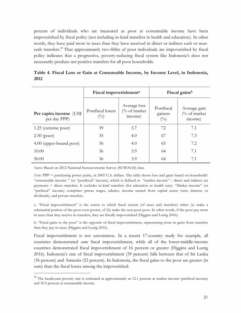
It is somewhat surprising—given that an average SUSENAS household in any decile is a fiscal policy net “winner”—that the rate at which fiscal policy makes individuals poor is significant. The figures for fiscal impoverishment and fiscal gains to the poor39 summarize how many of the poor lost or gained via the application of fiscal policy elements as well as the magnitudes of those losses or gains (table 4). When we define poverty as per capita income of less than US$1.25 per day PPP, after the fiscal instruments mentioned above are applied, nearly 40

39 See Higgins and Lustig (2016) for the elaboration of the fiscal impoverishment and fiscal gains to the poor indexes.

0%

10%

20%

30%

40%

50%

1 2 3 4 5 6 7 8 9 10

Shareofm

arketincom

e

disposableincomeconsumableincomefinalincome

21

percent of individuals who are measured as poor at consumable income have been impoverished by fiscal policy (not including in-kind transfers in health and education). In other words, they have paid more in taxes than they have received in direct or indirect cash or near-cash transfers.40 That approximately two-fifths of poor individuals are impoverished by fiscal policy indicates that a progressive, poverty-reducing fiscal system like Indonesia’s does not necessarily produce net positive transfers for all poor households.

Table 4. Fiscal Loss or Gain at Consumable Income, by Income Level, in Indonesia, 2012

Per capita income (US$ per day PPP)

Fiscal impoverishmenta Fiscal gainsb

Postfiscal losers

(%)

Average loss (% of market

income)

Postfiscal gainers

(%)

Average gain (% of market

income)

1.25 (extreme poor) 39 3.7 72 7.1

2.50 (poor) 35 4.0 67 7.3

4.00 (upper-bound poor) 36 4.0 65 7.2

10.00 36 3.9 64 7.1

50.00 36 3.9 64 7.1


Note: PPP = purchasing power parity, in 2005 U.S. dollars. The table shows loss and gains based on households’ “consumable income ” (or “postfiscal” income), which is defined as “market income” – direct and indirect tax payments + direct transfers. It excludes in-kind transfers (for education or health care). “Market income” (or “prefiscal” income) comprises pretax wages, salaries, income earned from capital assets (rent, interest, or dividends), and private transfers.

a. “Fiscal impoverishment” is the extent to which fiscal system (of taxes and transfers) either (a) make a substantial portion of the poor even poorer, of (b) make the non-poor poor. In other words, if the poor pay more in taxes than they receive in transfers, they are fiscally impoverished (Higgins and Lustig 2016).

b. “Fiscal gains to the poor” is the opposite of fiscal impoverishment, representing more in gains from transfers than they pay in taxes (Higgins and Lustig 2016).

Fiscal impoverishment is not uncommon. In a recent 17-country study for example, all countries demonstrated some fiscal impoverishment, while all of the lower-middle-income countries demonstrated fiscal impoverishment of 16 percent or greater (Higgins and Lustig 2016). Indonesia’s rate of fiscal impoverishment (39 percent) falls between that of Sri Lanka (36 percent) and Armenia (52 percent). In Indonesia, the fiscal gains to the poor are greater (in sum) than the fiscal losses among the impoverished. 40 The headcount poverty rate is estimated at approximately at 12.1 percent at market income (prefiscal income) and 10.5 percent at consumable income.

22

Equity of Fiscal Policy between Similar Households

As shown in table 4, some, but not all, poor households are impoverished by fiscal policy (excluding in-kind transfers). This finding indicates that horizontal equity (the degree to which individuals with similar income levels have similar transfer receipts and tax burdens) is incomplete. This incomplete horizontal equity limits the total redistributive effect of fiscal policy,41 and the overall redistributive effect of fiscal policy in Indonesia is small (as shown earlier in table 3). Table 5 quantifies the impact of incomplete horizontal equity on this redistributive effect.

Table 5 indicates that while reranking (RR, a measure of horizontal inequity) in Indonesia is relatively small, so too is the vertical equity (VE) component: RR is about two-fifths the size of VE in Indonesia, which is a larger relative share than in Brazil and South Africa, where fiscal policy has a much larger total redistributive effect (from market to postfiscal income). One of the consequences of Indonesia’s fiscal system—in which major transfers (energy subsidies) and taxes (VAT and excise taxes) are universal but do not cover everyone with equal net transfer amounts—is that some fiscal redistribution occurs between similar households.

Table 5. Redistributive, Vertical Equity, and Reranking Effects of Fiscal Policy in Indonesia Relative to Other CEQ Countries

Indicator

South Africa (2010)

Bolivia (2009)

Brazil (2009)

Indonesia

(2012)

Gini (market income)a 0.771 0.503 0.579 0.394

Gini (consumable income)b 0.695 0.503 0.546 0.391

Redistributive effectc 0.077 0.000 0.033 0.004

Vertical equity (VE)d 0.083 0.003 0.048 0.006

Reranking effect (RR)e 0.006 0.003 0.014 0.003

Horizontal inequity (RR/VE)f 0.075 1.000 0.300 0.418

Sources: Higgins and Pereira 2014 (Brazil); Paz-Arauco et al. 2014 (Bolivia); World Bank estimates based on 2012 National Socioeconomic Survey (SUSENAS) data (Indonesia). South Africa data from Inchauste, Lustig, Maboshe, Purfield, Woolard and ZIkhali (2017).

Note: CEQ = Commitment to Equity project. Indicators are calculated from income-based data for Bolivia, Brazil, and South Africa and from consumption-based data in the case of Indonesia. The Gini coefficient measures the inequality of income distribution. A value of 0 indicates full equality, and 1 indicates maximum inequality.

a. Market income comprises pretax wages, salaries, income earned from capital assets (rent, interest, or dividends), and private transfers. 41 For a more detailed discussion of vertical equity (VE), reranking (RR), and redistributive effects, see Inchauste and Lustig (2017) and Duclos and Araar (2006), (Inchauste, Lustig, Maboshe, Purfield, Woolard and Zikhali 2017).

23

b. Consumable income = market income − direct taxes and indirect taxes (value added and excise) + direct cash transfers + indirect subsidies.

c. The “redistributive effect” refers to the change in inequality associated with direct and indirect taxes as well as direct transfers and subsidies. It is calculated as the difference between the market income and consumable income Gini coefficients.

d. “Vertical equity” refers to the proportionality and progressivity of taxation, whereby the taxes paid increase with the amount of earned income.

e. The “reranking effect” is when fiscal interventions alter the relative position of individuals across the distribution (for example, if individual A was poorer than individual B before a fiscal intervention, but B is poorer than A after the intervention for no good reason).

f. “Horizontal inequity” refers to a situation where prefiscal and postfiscal income rankings are not preserved, calculated as the RR effect as a proportion of the VE effect, or RR/VE.

Fiscal policy has only a modest impact on the poverty headcount in Indonesia, but table 6 below shows that Indonesia is one of the rare CEQ countries where net indirect consumption taxes do not increase the poverty headcount (fiscal impoverishment notwithstanding). Net indirect subsidies are positive for every decile (as shown earlier in figure 1), meaning households in every decile collectively received more subsidy benefits (through consumption) than they paid in taxes (on consumption) on average.

Table 6. Poverty Headcount in Selected Countries, by Income Concept Percentage living on US$2.50 per person per day PPP

Country Market incomea Disposable incomeb Consumable incomec

Armenia (2011) 31.3 28.9 34.9

Bolivia (2009) 19.6 17.6 20.2

Brazil (2009) 15.1 11.2 16.3

Costa Rica (2010) 5.4 3.9 4.2

El Salvador (2011) 14.7 12.9 14.4

Ethiopia (2011) 81.7 82.4 84.2

Guatemala (2010) 35.9 34.6 36.5

Indonesia (2012) 56.4 55.9 54.9

Mexico (2010) 12.6 10.7 10.7

Peru (2009) 15.2 14.0 14.5

South Africa (2010) 46.2 33.4 39.0

Uruguay (2009) 5.1 1.5 2.3

Sources: Beneke, Lustig, and Oliva, 2018 (El Salvador); Bucheli et al. 2014 (Uruguay); Cabrera, Lustig, and Morán 2015 (Guatemala); Higgins and Pereira 2014 (Brazil); Jaramillo 2014, 2015 (Peru); Paz-Arauco et al. 2014 (Bolivia); Sauma and Trejos 2014 (Costa Rica); Scott 2014 (Mexico). World Bank estimates based on 2012 National

24

Socioeconomic Survey (SUSENAS) data (Indonesia). Armenia, Ethiopia, and South Africa data from Younger and Khachatryan (2017), Hill, Inchauste, Lustig, Tsehaye and Woldehanna (2017) and Inchauste, Lustig, Maboshe, Purfield, Woolard and ZIkhali (2017), respectively.

Note: PPP = purchasing power parity, in 2005 U.S. dollars.

a. Market income comprises pretax wages, salaries, income earned from capital assets (rent, interest, or dividends), and private transfers.

b. Disposable income = market income – direct taxes + direct cash transfers.

c. Consumable income = disposable income − indirect taxes (value added and excise) + indirect subsidies.

Marginal Contributions of Fiscal Policy Elements to Income Redistribution

The Kakwani progressivity index for taxes and transfers indicates that only two spending items (pension income and tertiary education spending) are regressive in Indonesia, while only the tobacco excise tax is absolutely regressive (table 7).42 Civil servant pensions were not designed as a social policy instrument but are a nonsalary benefit for government employees; and regressivity in tertiary education expenditures is driven by enrollment—the small number of students reaching the tertiary level are disproportionately nonpoor—rather than by program design.

42 Table 7 shows the marginal impact of pension income. For the pension system (that is, the cumulative impact of pension contributions made by households and pension benefits received by households) the marginal impact on inequality reduction is positive (at disposable, consumable, and final income). The VAT regime does include exemptions for basic foodstuffs, public transport, and other necessities and is likely better described as “neutral,” rather than regressive, in both design and operation. Furthermore, the Kakwani index for total indirect taxes is approximately zero, indicating a neutral indirect tax regime. (For a further explanation of the Kakwani index, see Inchauste and Lustig [2017]).

25

Table 7. Marginal Contributions of Expenditures and Taxes to Inequality Reduction in Indonesia, 2012

Fiscal intervention

Kakwanie

Magnitude (% of GDP)

Marginal inequality reduction, from market incomea

Disposable incomeb

Consumable incomec

Final incomed

Redistributive effect n.a. n.a. 0.0043 0.0036 0.0237

Contributory pensionf −0.209 0.76 0.0002 0.0001 −0.0001

Direct transfers 0.640 0.33 0.0042 0.0041 0.0037

PKH 0.854 0.02 0.0008 0.0008 0.0007

Scholarships 0.669 0.08 0.0003 0.0003 0.0003

Rasking 0.596 0.23 0.0030 0.0030 0.0028

Indirect taxes −0.042 5.3 n.a. −0.0031 −0.0022

VAT 0.015 4.1 n.a. 0.0010 0.0015

Tobacco excise −0.134 1.2 n.a. −0.0043 −0.0038

Indirect subsidies 0.056 3.7 n.a. 0.0026 0.0014

In-kind education 0.363 2.7 n.a. n.a. 0.0193

Primary 0.471 0.85 n.a. n.a. 0.0089

Junior Secondary 0.425 1.05 n.a. n.a. 0.0083

Senior Secondary 0.288 0.34 n.a. n.a. 0.0023

Tertiary −0.085 0.37 n.a. n.a. −0.0007

In-kind health 0.273 0.89 n.a. n.a. 0.0031


Note: n.a. = not applicable. PKH = Hopeful Family Program (Program Keluarga Harapan). VAT = value added taxes.


b. Disposable income = market income − payments for personal income taxes + direct cash transfers.

c. Consumable income = disposable income – indirect taxes (VAT and excises) + indirect subsidies.

d. Final income = consumable income + value of in-kind transfers (such as for education and health care).

e. The Kakwani coefficient is a typical measure of progressivity, using market income as the base. For taxes, it is the difference between the concentration coefficient of the tax and the Gini for market income. For transfers, it is

26

the difference between the Gini for market income and the concentration coefficient of the transfer. (See Inchauste and Lustig [2017] for a further explanation).

f. The marginal contribution of the contributory pension system is the cumulative impact of pension contributions made by households and pension benefits received by households. The marginal impact of pension benefits by themselves is negative, meaning income inequality is higher when pension income is added.

g. The Raskin rice subsidy program is treated as a direct cash transfer because the subsidized rice distributed through the program is often resold for cash.

Table 7 also summarizes marginal impacts on inequality (as summarized by the Gini coefficient) along with the magnitude of tax revenues collected or transfer expenditures made. Direct transfers—PKH, Raskin, and Poor Student Education Support (BSM)—collectively have a larger marginal impact on inequality than do energy subsidies, but subsidies receive a budget allocation that is 10 times the allocation for direct transfers. Likewise, education (cumulatively) has an impact on inequality more than 10 times the impact of energy subsidies, but subsides receive a budget allocation that is one-third again as large as that for education. Inequality is neither much increased nor decreased even though most policy instruments available do reduce inequality.

Cash and near-cash transfers, energy subsidies, and in-kind transfers (in health and education) are all progressive with respect to market income. But notice that transfers provided via subsidy spending or in-kind provision of services are received indirectly through consumption, which means that households consuming either more (as in the case of energy subsidies) or higher-valued types (as in the case of tertiary education or health) will receive proportionately larger shares of the transfers available.

Indonesia’s direct transfers do reduce poverty by approximately 1 percentage point although little is spent on them (table 8). Within the set of direct transfers, the subsidized rice program’s (Raskin) impact on poverty is two to three times that of PKH although the expenditures are over 10 times as high.

The same pattern happens across transfer types as well: although energy subsidies’ impact on poverty reduction (4 percentage points) is approximately four times the impact of direct transfers (1 percentage point), the budget allocation for subsidies exceeds the budget allocation for direct transfers by a factor greater than 10. So, not all poor households are covered by direct transfer initiatives, and direct transfer beneficiaries receive amounts that are small (relative to their own incomes); consequently the impact on poverty from direct transfer expenditures is modest. The impact on poverty is greater from energy subsidy programs, but the magnitudes of those subsidy expenditures are several times greater (proportionally) than are direct transfer magnitudes.

27

Table 8. Marginal Contributions of Transfers, Taxes, and Subsidies to Poverty Reduction in Indonesia, 2012

Fiscal intervention


Marginal poverty reduction, from market incomea

Disposable incomeb

Consumable incomec

Poverty reduction impact (at income of US$1.25 per day PPP)

n.a. 0.0124 0.0153

Direct transfers 0.33 0.0118 0.0113

PKH 0.02 0.0025 0.0027

Scholarships 0.08 0.0012 0.0011

Raskind 0.23 0.0079 0.0081

Indirect taxes 5.3 n.a. −0.0273

VAT 4.1 n.a. −0.0145

Tobacco excise 1.2 n.a. −0.0157

Indirect subsidies 3.7 n.a. 0.0410


Note: n.a. = not applicable. PPP = purchasing power parity (in 2005 U.S. dollars). PKH = Hopeful Family Program (Program Keluarga Harapan). VAT = value added taxes.




d. The Raskin rice subsidy program is treated as a direct cash transfer because the subsidized rice distributed through the program is often resold for cash.

Effect of Social Spending on Incomes

We generate Beckerman-Immervoll efficiency indexes for marginal poverty reduction contributions (from market to disposable income) in table 9. The vertical expenditure efficiency (VEE) indicator shows that less than one quarter of total direct cash benefits available (PKH, BSM, Raskin) are transferred to the poor (at the national poverty line). The larger transfers (BSM and Raskin) both have target beneficiaries defined as eligible households or individuals who are “poor or near poor,” so we also look at VEE at the national

28

vulnerability line: nearly two-fifths (37 percent) of direct transfers reach the moderate-poverty-line poor.43

Table 9. Direct Transfers and Poverty Reduction

Beckerman-Immervoll indicator

National poverty linea

National vulnerability lineb

VEE 0.22 0.37

S 0.12 0.06

PRE 0.20 0.35

Change in poverty rate (%) −1.3 −1.3

PGE 0.16 0.10

Change in poverty gap (%)c −0.4 −0.5


Note: VEE = vertical expenditure efficiency, the percentage of direct transfers that go to the poor. S = spillover, the share of transfer expenditures that move households over the poverty line, thus benefiting those who are no longer poor. PRE = poverty reduction effectiveness, the percentage of reduction in the poverty headcount rate. PGE = poverty gap efficiency, the extent to which transfers cover the gap between poor households’ incomes and the poverty line (Beckerman 1979; Immervoll et al. 2009).

a. The 2014 national poverty line was expenditure of about Rp 302,735 (US$25) per person per month.

b. The 2014 national vulnerability line is 1.5 times the poverty line, or Rp 454,103 per person per month (US$37.50).

c. The poverty gap is the average percentage by which poor individuals fall below a given poverty line.

The spillover (S) index, at 0.12, indicates that direct-transfer magnitudes rarely exceed the strictly necessary amount required for poor beneficiaries to reach poverty-line income; in other words, transfer levels are appropriately specified given coverage. 44 The poverty reduction effectiveness (PRE) indicator, which is the product of VEE times (1−S), shows that in Indonesia only 20 percent of direct transfer spending actually helped reduce the headcount poverty rate, and only 35 percent helped to reduce the vulnerability rate. The poverty gap efficiency (PGE) indicator shows that in Indonesia the distribution of direct transfers eliminates 16 percent of the (pretransfer) poverty gap. Indonesia’s PGE confirms two weaknesses constraining the impact of direct transfers on poverty reduction: coverage is low, meaning the majority of poor households’ incomes or expenditures are unchanged after direct transfers are distributed; and transfer values are small for those who actually receive them. 43 The “national poverty line” in Indonesia is calculated by expenditure level rather than income level. As of 2014, the poor were those living below expenditure of about Rp 302,735 (US$25) per person per month (Aji 2015; World Bank 2016). The “national vulnerability line” is set at 1.5 times the poverty line, or Rp 454,103 per person per month (US$37.50). 44 However, the objective of Indonesian social assistance programs is not solely to put the poor over the poverty line; that is, they are not designed to have no “spillover.”

29

Ultimately, households in the poorest decile receive direct transfers, indirect subsidies, and in-kind transfers that are worth 30 percent of their market income; indirect taxes represent about 7 percent of their market income. So, in net terms—and again for the poorest decile—direct transfers boost market income by approximately 4 percent, net subsidies provide a boost of approximately 2 percent, and net in-kind transfers provide a boost of approximately 19 percent.45 For the richest decile, the analogous numbers are 0.05 percent, 1.0 percent, and 3.0 percent—meaning that the survey households in the richest decile are cumulative recipients of public expenditures rather than net contributors to public revenues (as shown earlier in figure 1).

In-Kind Transfers and the Distribution of Utilization

In-kind transfers of health and education services are the largest social expenditures we consider; the only other public expenditure category of commensurate magnitude is subsidies. Because receipt of in-kind transfers requires use of the services provided, and we value those services at the (uniform, average) cost to the government of providing them, the redistributive effect of this set of transfers is driven entirely by the distribution of use: if certain income groups use the service with greater frequency (or if they consume higher-valued types of the public service with greater frequency), they will receive greater shares of total in-kind expenditures.

Enrollment rates are high for all income groups in Indonesian primary schools and then decline rapidly for lower-income students from primary to lower-secondary; from lower- to upper-secondary; and from upper-secondary to tertiary (figure 2). The rate of tertiary enrollment in the poorest three deciles is essentially zero; while few SUSENAS individuals overall are enrolled in tertiary education. Nearly 100 percent of those enrolled in tertiary education come from households with at least median per capita incomes. Use of health care services, on the other hand, is distributed approximately uniformly across income deciles (figure 3).

45 Because indirect taxes and public service access fees are a burden (and subsidies and in-kind benefit transfers become a benefit) conditional on consumption, it is easier to express indirect subsidies or taxes and in-kind transfers or access fees in “net” terms.

30

Figure 2. Gross School Enrollment Rates in Indonesia, by Income Decile, 2012


Figure 3. Health Care Service Utilization Rates in Indonesia, by Income Decile, 2012


As table 7, indicated earlier, cumulative public education services do reduce inequality, but the results vary noticeably by education level.46 For example, the marginal impact of primary and

46 The private education sector in Indonesia also benefits from public education spending primarily through the placement of civil servant teachers (provided to all education levels) and an “operational funds” budget that is

0%

20%

40%

60%

80%

100%

SD SMP SMU Tertiary

Perc

enta

ge o

f Sc

hool

-age

enr

olle

d

Poorest Decile Richest Decile

0%5%10%15%20%25%30%35%40%45%

Poorestdecile

2 3 4 5 6 7 8 9 Richestdecile

Percen

tageofD

ecileReceivingHealth

Be

nefits

31

lower-secondary education transfers are estimated to be nearly 1 percentage point, while for upper-secondary the estimated marginal impact is closer to 0.2 percentage points. Tertiary education expenditures have a negative estimated marginal impact which is nevertheless small (at less than 0.1 percentage point). This across-education-levels pattern can be predicted from figure 2, which shows that education utilization gaps between poorer and richer households are smallest for primary education and grow steadily larger from lower-secondary to tertiary levels. Public health services provided have a positive marginal impact on inequality, but the impact is smaller than that for education.

Most individuals using public health and education services in Indonesia pay non-negotiable fees to access those systems; such fees are most often charged by the unit providing the service (such as the school, hospital, or clinic). This practice indicates that centrally provided public expenditures do not completely cover the locally prevailing inclusive cost of public provision. Our baseline scenario treats them as excise taxes (levied at the public service provider), while the centrally budgeted expenditures accruing to a particular service are treated as a subsidy, so that to each public health care or education service accrues a “net” subsidy (equal to the central-level unit subsidy minus the local-level tax). 47 It is this “net” subsidy that was summarized earlier in table 8 and in the text preceding table 7.

We can also treat the payment of non-negotiable, unregulated fees as disposable income (which would have been spent in the same amounts and on the same services in the absence of public expenditures on the same services). Theoretically, these “membership” or access fees are unrelated to the central government’s cost of providing the health care or education services utilized.48 When we treat these fees as the price of access to the public provision system (rather than as an indirect tax on the consumption of public services), we can then also provide to households the full cost of provision of public services (rather than the “net” subsidy as described above); our third sensitivity analysis does exactly that.

provided on a per-student basis to both private and public education providers at the primary and lower-secondary levels. 47 An implication of this scenario is that households or individuals acquiring public services value the service acquired at some level higher than the central government’s cost of provision; the “tax” paid by service-utilizing individuals is treated as revenue by the government. 48 This alternative scenario may capture a form of “insurance” provided by the fee-collecting institution. Theories of administrative and political decentralization propose that local-level actors have more and higher-quality information regarding local preferences and budgets on both the supply and demand sides of any transaction. Indonesia’s fee system—which is a burden on users only and which allows for price discrimination under limited competition—can be regarded as a locally determined and affordable “premium” charged to likely users that ensures the continued effective operation of the facilities users visit. The costs of “continued effective operation” include (but are not limited to) capital depreciation as well as maintaining a sufficient labor productivity level. (Under limited competition, skilled health care service labor will have outside options). In other words, the fees charged to users insure those same users against decreasing productivity or the facility going offline altogether. If the fees charged do accomplish this insurance function, then in the event that such fees were abolished, the poverty headcount (as measured by expenditure levels) would not necessarily change although health status might decline (on average), leading to lower broadly measured welfare, particularly among those households unable to afford the nonsubsidized cost of provision.

32

To summarize this alternative conceptualization (which forms one of the sensitivity analyses in our analytical framework), table 10 presents the Gini and concentration coefficients for the distribution of disposable income before and after these fees are paid as well as the distribution of the in-kind health and education transfers with respect to disposable income.

Table 10. Marginal Contributions of In-Kind Transfers to Inequality Reduction in Indonesia, by Income Concept, 2012

In-kind transfer type

Kakwanie


Marginal inequality reduction, from market incomea

Disposable incomeb

Consumable incomec

Final incomed

Redistributive effect

In-kind fees as tax n.a. n.a. 0.0043 0.0036 0.0237

In-kind fees as income n.a. n.a. 0.0051 0.0044 0.0258

In-kind fees as income

Public health fees 0.271 0.15 0.0019 0.0019 0.0020

Public education fees −0.170 0.52 −0.0027 −0.0026 −0.0009

In-kind public spending

In-kind health spending 0.284 0.9 n.a. n.a. 0.0028

In-kind education spending 0.361 2.7 n.a. n.a. 0.0174

All in-kind spending + fees 0.495 4.2 n.a. n.a. 0.0197






d. Final income = consumable income + value of in-kind transfers (such as for education and health care).

e. The Kakwani coefficient is a typical measure of progressivity, using market income as the base. For taxes, it is the difference between the concentration coefficient of the tax and the Gini for market income. For transfers, it is the difference between the Gini for market income and the concentration coefficient of the transfer. (For further explanation, see Inchauste and Lustig [2017]).

33

Public education access fees have a negative Kakwani coefficient, indicating that those with higher income shares pay decreasing shares of these fees. This result is due in part to a higher rate of private education among richer households: fees paid for privately provided education do not contribute to public revenues and therefore cannot be turned into public expenditures. Fees paid for public health system access are progressively distributed and pro-poor in that the fee shares are smaller (for all but the richest decile) than market income or disposable income shares.49

The Gini coefficient on disposable income measured without these public service fees included is approximately three-tenths of a percentage point higher (at 0.3934) than the Gini coefficient on disposable income measured with public service fees included (0.3899). This indicates that the reduction in the Gini coefficient is larger when these fees are levied; without public health and education service access fees, measured inequality (at disposable income) would be greater.50

5. Conclusions

This report assesses the distributional impact of a subset of the public revenue collection and spending instruments and finds that fiscal policy does reduce both poverty and inequality in Indonesia. However, the magnitudes are modest. Indonesian fiscal policy does not harm many individuals: fiscal impoverishment is low when in-kind transfers are included. However fiscal impoverishment is much higher when we examine only those tax and expenditure instruments that have a direct impact on consumable income: nearly 40 percent of poor individuals (at post-fiscal, consumable income) have been impoverished by fiscal policy.

We have allocated just over 70 percent of total tax revenue collected from households (and about 44 percent of total tax revenues) including VAT and excise taxes; PIT burdens are expected to be zero for SUSENAS households. We have allocated 56 percent of primary government expenditures with a focus on social spending including direct cash transfers, health and education spending, and non-social fuel subsidy spending.

49 Some individuals may not be accessing health care service providers because of anticipated fees. If individuals constrained in this way are more often from poorer deciles, poorer households bear a greater burden (from these fees) than the statistics in table 10 indicate. The SUSENAS household survey does not allow us to identify individuals who did not visit health care providers because of anticipated fees. The same caveats apply to fees charged by public education providers. 50 Inequality (as measured by the Gini coefficient) is slightly lower at final income under this alternative scenario than under our benchmark case (where public service fees are treated as an indirect tax on public service consumption), shown earlier in table 3. This result is logical because, in the alternative scenario, we do not remove the equalizing effect of the public service fees through their characterization as an indirect tax.

34

Summary of Fiscal Impacts

Indonesia’s (2012-era) fiscal policy reduced poverty and inequality through a slightly regressive indirect tax system and slightly progressive social spending. Everyone in Indonesia contributes consumption-based tax revenues, and those resources are redistributed as government expenditure on direct and indirect transfers and in-kind spending that raises incomes for everyone—raising incomes for the poorest individuals proportionately more than for the richest individuals. Approximately 3.6 million individuals were lifted out of poverty (at the US$2.50 or US$1.25 per day PPP lines or at the prevailing national poverty line) as a result of the tax-and-transfer system.

Fiscal resources are replenished with household contributions, mainly from taxes on consumption. Total consumption taxes actually increase inequality (marginally). The larger of the taxes (VAT) has a positive marginal impact on inequality while the smaller tobacco excise has a negative marginal impact on inequality. Kakwani coefficients (as shown in table 7) indicate that VAT is progressively distributed (with respect to market income): the share of total VAT paid rises with market income.

Direct transfers are equalizing and more effectively target the poor than in-kind transfers or subsidies. They are also quite small in magnitude—total spending on all direct transfers representing less than half a percentage point of GDP—and either provide relatively small benefit packages or do not have very broad coverage (or both). The marginal inequality and poverty reduction impacts of these direct transfers are therefore muted.

In-kind benefits, which are much larger in both expenditure and coverage magnitudes, are received only by individuals using a publicly provided service. Poorer households in Indonesia have far lower rates of access to secondary- and tertiary-level education (and approximately equal rates of access to health care services) than do rich households. Even so—and because the lower-cost types of such public services (elementary education or outpatient health care, for example) have positive marginal inequality reduction impacts—overall the public provision of services, and especially the provision of basic education, are equalizing. The combination of social spending (direct and in-kind transfers) and energy subsidies is modestly inequality- and poverty-reducing.

Energy subsidies and education spending alone account for approximately 80 percent of all public expenditures analyzed here. Energy subsidies in 2012 had a positive marginal impact on inequality reduction. As a consequence, the resulting net subsidy on consumption (subsidies received through consumption minus taxes paid through consumption) is slightly progressive (with respect to disposable income) and poverty-reducing. Because very few individuals pay more in taxes than they receive in transfers, Indonesia’s fiscal system boosts market income (on average) not just among poor households, but also among middle-income and rich households.

35

CEQ Comparison and Policy Implications

Compared with the rest of the CEQ country set, Indonesia has relatively low prefiscal inequality (in terms of market income). However, Armenia and Ethiopia (for example), which have similarly low prefiscal inequality, surpass Indonesia in terms of poverty or inequality reduction through fiscal policy while spending similarly low amounts.

The particularly modest impacts on inequality and poverty of Indonesia’s fiscal practices have to do in part with a low revenue base: Indonesia’s PIT collections and the effective indirect tax rate (on consumption) are both low by CEQ-country standards. These modest impacts also stem from Indonesia’s prioritization of energy subsidies: its untargeted energy subsidies have broad coverage among poor, middle-income, and rich households and account for total expenditures more than 10 times as large as the country’s direct transfers. Regardless of the optimal magnitude of fiscal expenditures in Indonesia, then, policy makers can still reduce income equality and reduce the number of impoverished citizens by shifting fiscal priorities away from untargeted subsidies and toward targeted transfers.

36

References

Afkar, Rythia, Jon Jellema, and Matthew Wai-Poi. 2015. “CEQ Master Workbook: Indonesia. Version: March 15, 2015.” Commitment to Equity (CEQ) Data Center, CEQ Institute, Tulane University, New Orleans.

Aji, Priasto. 2015. “Summary of Indonesia’s Poverty Analysis.” ADB Papers on Indonesia No. 4. Asian Development Bank, Manila.

Beckerman, W. 1979. “The Impact of Income Maintenance Payments on Poverty in Britain, 1975.” Economic Journal 89 (354):261–79.

Beneke, Margarita, Nora Lustig, and Jose Andres Oliva. 2018. "The Impact of Taxes and Social Spending on Inequality and Poverty in El Salvador." Chapter 15 in Commitment to Equity Handbook. Estimating the Impact of Fiscal Policy on Inequality and Poverty, edited by Nora Lustig (Brookings Institution Press and CEQ Institute, Tulane University). Advance online version available at http://www.commitmentoequity.org/publications/handbook.php.

Bibi, Sami, and Jean-Yves Duclos. 2010. “A Comparison of the Poverty Impact of Transfers, Taxes and Market Income across Five OECD Countries.” Bulletin of Economic Research 62 (4):387–406.

BPK (Audit Board of the Republic of Indonesia), Laporan Keuangan Pemerintah Pusat Tahun 2012, Annual audit report BPK, (Jakarta, 2013), http://www.bpk.go.id/lkpp.

BPS Statistics Indonesia, National Socioeconomic Survey, (Jakarta, 2012), http://microdata.bps.go.id/mikrodata/index.php/catalog/SUSENAS.

Bucheli, Marisa, Nora Lustig, Maximo Rossi, and Florencia Amabile. 2014. "Social Spending, Taxes and Income Redistribution in Uruguay." The Redistributive Impact of Taxes and Social Spending in Latin America. Special Issue, Public Finance Review 42 (3):413-433. doi: http://dx.doi.org/10.1177%2F1091142113493493.

Maynor, Cabrera, Lustig Nora, and Hilcias E. Moran. 2015. "Fiscal Policy, Inequality, and the Ethnic Divide in Guatemala." World Development 76 (December):263-279. doi: 10.1016/j.worlddev.2015.0.

Damuri, Yose Rizal, and Ari A. Perdana. 2003. “The Impact of Fiscal Policy on Income Distribution and Poverty: A Computable General Equilibrium Approach for Indonesia.” Economics Working Paper No. WPE068. Center for Strategic and International Studies (CSIS), Jakarta, Indonesia.

Dartanto, Teguh. 2013. “Reducing Fuel Subsidies and the Implication on Fiscal Balance and Poverty in Indonesia: A Simulation Analysis.” Energy Policy 58 (July 2013):117–34.

37

Duclos, Jean-Yves, and Abdelkrim Araar. 2006. Poverty and Equity: Measurement, Policy, and Estimation with DAD. New York: Springer and International Development Research Centre.

Hadiwibowo, Yuniarto. 2010. “Fiscal Policy, Investment and Long-Run Economic Growth: Evidence from Indonesia.” Asian Social Science 6 (9):3–11.

Higgins, Sean, and Nora Lustig. 2016. "Can a Poverty-reducing and Progressive Tax and Transfer System Hurt the Poor?" Journal of Development Economics 122 (September):63-75. doi: 10.1016/j.jdeveco.2016.04.001.

Higgins, Sean, and Claudiney Pereira. 2013. "The Effects of Brazil’s High Taxation and Social Spending on the Distribution of Household Income." The Redistributive Impact of Taxes and Social Spending in Latin America. Special Issue, Public Finance Review 42 (3):346–67. doi: 10.1177/1091142113501714.

Hill, Ruth, Gabriela Inchauste, Nora Lustig, Eyasu Tsehaye and Tassew Woldehanna. 2017. “A Fiscal Incidence Analysis for Ethiopia,” in The Distributional Impact of Fiscal Policy: Experience from Developing Countries, edited by Gabriela Inchauste and Nora Lustig Washington DC: World Bank.

Immervoll, Herwig, Horacio Levy, José Ricardo Nogueira, Cathal O’Donoghue, and Rozane Bezerra de Siqueira. 2009. “The Impact of Brazil’s Tax-Benefit System on Inequality and Poverty.” In Poverty, Inequality, and Policy in Latin America, edited by Stephan Klasen and Felicitas Nowak-Lehmann, 271–301. Cambridge, MA: MIT Press.

Inchauste, Gabriela and Nora Lustig. 2017. “Overview: Fiscal Policy and Redistribution." In The Distributional Impact of Fiscal Policy: Experience from Developing Countries, edited by Gabriela Inchauste and Nora Lustig. Washignton DC: World Bank.

Inchauste, Gabriela, Nora Lustig, Mashekwa Maboshe, Catriona Purfield, Ingrid Woolard and Precious Zikhali. 2017. “The Distributional Impact of Fiscal Policy in South Africa,” in The Distributional Impact of Fiscal Policy: Experience from Developing Countries, edited by Gabriela Inchauste and Nora Lustig. Washington DC: World Bank.

Jaramillo, Miguel. 2014. “The Incidence of Social Spending and Taxes in Peru.” The Redistributive Impact of Taxes and Social Spending in Latin America. Special Issue, Public Finance Review 42 (3):391–412.

———. 2015. "CEQ Master Workbook: Peru. Version: August 7, 2015." CEQ Data Center (CEQ Institute, Tulane University).

Jellema, Jon, and Hassan Noura. 2012. “Protecting Poor and Vulnerable Households in Indonesia.” Public Expenditure Review. World Bank, Washington, DC.

38

Lustig, Nora. 2016. "Fiscal Policy, Inequality and the Poor in the Developing World." Commitment to Equity (CEQ) Working Paper Series 23. Tulane University, Department of Economics, October.

———, ed. 2018. Commitment to Equity Handbook. Estimating the Impact of Fiscal Policy on Inequality and Poverty. (Brookings Institution Press and CEQ Institute, Tulane University). Advance online version available at http://www.commitmentoequity.org/publications/handbook.php.

Lustig, Nora, and Sean Higgins. 2013. "Commitment to Equity Assessment (CEQ): Estimating the Incidence of Social Spending, Subsidies and Taxes. Handbook." CEQ Working Paper 1. Center for Inter-American Policy and Research and Department of Economics, Tulane University and Inter-American Dialogue, September.

Paz Arauco, Veronica, George Gray Molina, Wilson Jimenez Pozo, and Ernesto Yanez Aguilar. 2013. "Explaining Low Redistributive Impact in Bolivia." The Redistributive Impact of Taxes and Social Spending in Latin America. Special Issue, Public Finance Review 42 (3). doi: 10.1177/1091142113496133.

Sauma, Pablo, and Juan Diego Trejos. 2014. "Social Public Spending, Taxes, Redistribution of Income, and Poverty in Costa Rica." CEQ Working Paper 18. Center for Inter-American Policy and Research and Department of Economics, Tulane University and Inter-American Dialogue, March.

Scott, John. 2014. "Redistributive Impact and Efficiency of Mexico’s Fiscal System." The Redistributive Impact of Taxes and Social Spending in Latin America. Special Issue, Public Finance Review 42 (3):368-390. doi: 10.1177/1091142113497394.

Theil, H. 1967. Economics and Information Theory. Chicago: Rand McNally and Company.

Wai-Poi, Matthew, Monica Wihardja, and Michaelino Mervisiano. Forthcoming. “The Problem with Taxes: Estimating Top Incomes in Indonesia.” Working Paper. World Bank, Jakarta.

Inchauste, Gabriela, Nora Lustig, Mashekwa Maboshe, Catriona Purfield, Ingrid Woolard, and Precious Zikhali. 2016. "CEQ Master Workbook: South Africa. Version: March 6, 2016." CEQ Data Center (CEQ Institute, Tulane University and the World Bank).

World Bank. 2016. “Indonesia’s Rising Divide: Why Inequality Is Rising, Why It Matters and What Can Be Done.” Research project report. World Bank, Jakarta.

Younger, Stephen D. and Artsvi Khachatryan. 2017. “Fiscal Incidence in Armenia,” in The Distributional Impact of Fiscal Policy: Experience from Developing Countries, edited by Gabriela Inchauste and Nora Lustig. Washington DC: World Bank.

Documents

THE DISTRIBUTIONAL IMPACT OF FISCAL POLICY IN … · THE DISTRIBUTIONAL IMPACT OF FISCAL POLICY IN INDONESIA* Jon Jellema, Matthew Wai-Poi, and Rythia Afkar† CEQ Working Paper 40