THE EFFECT OF ANTHROPOGENIC EMISSIONS ON THE …

www.tjprc.org [email protected]

THE EFFECT OF ANTHROPOGENIC EMISSIONS ON THE RECENT RISE IN

GLOBAL TEMPERATURE ANOMALIES

SARVA SANJAY

Student IBDP-2, Podar International School, Mumbai, India

ABSTRACT

Climate change is one of the most important issues currently facing mankind. One of the most important questions is

determining the extent of climate change as well as the extent to which human activities cause climate change.

Determining the answer to this question has important ramifications in shaping policy decisions to curb carbon

emissions. The goal of this paper is to establish a relationship between the net human contribution to atmospheric

carbon dioxide and the global temperature anomaly. To do this, we first form a climate model describing the relations

between carbon dioxide concentration in the atmosphere and the temperature anomaly. Then we examine the

components of the global carbon budget and form an expression for the human contribution to atmospheric carbon

dioxide. In our results section, we use data from various databases to confirm the relation between carbon dioxide

concentration and temperature anomalies; compare the projected gain in atmospheric carbon dioxide and the actual

growth and construct a relation between the net human contribution to atmospheric carbon dioxide and temperature

anomalies. We observe that there exists a strong correlation between the human contribution and the increasing

temperature anomalies which is logarithmic in nature. Finally, we elaborate on any errors or uncertainties in our data.

KEYWORDS: Anthropogenic, Global Temperature & Anomalies

Received: Aug 26, 2021; Accepted: Sep 16, 2021; Published: Sep 27, 2021; Paper Id.: IJPRDEC20215

INTRODUCTION

The purpose of this paper is to confirm a correlation between the increase in global temperatures to anthropogenic

emissions. For this, we do not use global mean temperatures as actual temperature measurements are difficult to

gather from all places over the globe. Instead, we use global temperature anomalies which refers to the departure of

global temperatures from a reference value. We prefer to use temperature anomalies over mean temperatures as

they are easier to measure and produce a greater accuracy over a larger area. We also cannot directly human

emissionsas there exist both land and ocean sinks which absorb carbon dioxide and whose values vary with time.

As not all human emission are absorbed by the atmosphere, we shall be evaluating the net anthropogenic

contribution to atmospheric carbon dioxide i.e. the amount of human emissions which are released into the

atmosphere after being absorbed by ocean and land sinks. Hence my research question is

“How does the global temperature anomaly vary with the net anthropogenic contribution to atmospheric

carbon dioxide?”.

In order to answer this question, we must divide it into two parts (1) What is the relation between carbon

dioxide concentration in the atmosphere and temperature anomaly? (2) How much of the growth in atmospheric

carbon dioxide can be attributed to human activities? In order to answer these questions, we must develop a climate

model as well as a carbon budget and then compare data using existing databases to see whether the data matches

Orig

ina

l Article

International Journal of Physics

and Research (IJPR)

ISSN (P): 2250–0030; ISSN (E): 2319–4499

Vol. 11, Issue 2, Dec 2021, 43–58

© TJPRC Pvt. Ltd.

44 Sarva Sanjay

Impact Factor (JCC): 4.8905 NAAS Rating: 4.00

with the model developed.

THEORY

One of the reasons why carbon dioxide plays a unique role in the increase in global temperatures is due to its unique

structure and spectroscopy. A gas molecule absorbs radiation of a particular wavelength only if the energy absorbed can be

used to increase the internal energy of the molecule. This is achieved through a transition from a lower to higher state.

Since these states within a molecule are discrete, molecules can only absorb radiations of certain wavelengths. These

transitions could either be electronic, which require high energy radiations from the ultraviolet spectrum, or vibrational,

which require low energy radiations from the far-infrared spectrum. Some absorption can also take place due to rotational

transitions in the near-infrared spectrum1.

The vibrational state of a CO2 molecule is defined by a combination of three normal vibrational modes and by a

quantized energy level within each mode. Vibrational transitions involve changes in the energy level (vibrational

amplitude) of one of the normal modes. In the "symmetric stretch" mode the CO2 molecule has no dipole moment, since

the distribution of charges is perfectly symmetric; transition to a higher energy level of that mode does not change the

dipole moment of the molecule and is therefore forbidden. Changes in energy levels for the two other, asymmetric, modes

change the dipole moment of the molecule and are therefore allowed. In this manner, CO2 has absorption lines in the near-

IR. Contrast the case of N2 . The N2 molecule has a uniform distribution of charge and its only vibrational mode is the

symmetric stretch. Transitions within this mode are forbidden, and as a result, the N2 molecule does not absorb in the near-

IR.

More generally, molecules that can acquire a charge asymmetry by stretching or flexing (CO2, H2O, N2O, O3,

hydrocarbons...) are greenhouse gases; molecules that cannot acquire charge asymmetry by flexing or stretching (N2, O2,

H2) are not greenhouse gases. Atomic gases such as the noble gases have no dipole moment and hence no greenhouse

properties. Examining the composition of the Earth's atmosphere, we see that the principal constituents of the atmosphere

(N2, O2, Ar) are not greenhouse gases. Most other constituents, found in trace quantities in the atmosphere, are greenhouse

gases. The important greenhouse gases are those present at concentrations sufficiently high to absorb a significant fraction

of the radiation emitted by the Earth; the list includes CO2, H2O, N2O, O3 and chlorofluorocarbons (CFCs). By far the most

important greenhouse gas is water vapor because of its abundance and its extensive IR absorption features.

By plotting the efficiency of absorption of radiation by the atmosphere we can see that, the atmosphere is nearly

100% opaque in the UV spectrum due to electronic transitions in O2 and O3 and nearly transparent to the visible spectrum.

The efficiency once again increases to 100% at IR wavelengths due to greenhouse gases. Therefore, we can conclude that

greenhouse gases play a significant role in the warming of the atmosphere as most of the absorption by the atmosphere is

by greenhouse gases.

We must now model the atmosphere taking into account the heating caused due to the greenhouse effect for which

we need to make a few assumptions about the structure and behaviour of the atmosphere. We neglect any absorption in the

visible spectrum by the atmosphere. We also assume thermodynamic equilibrium which means that alocalised atmospheric

volume below 40kms is considered to be isotropic (emissions are non-directional) with uniform temperature.We define the

effective emission temperature to be the temperature of the Earth in the absence of an atmosphere, only taking into account

1Jacob, Daniel. Introduction to Atmospheric Chemistry. Illustrated, Princeton University Press, 1999.

The Effect of Anthropogenic Emissions on the Recent Rise in Global Temperature Anomalies 45


its reflectivity and its distance from the Sun. As the rate of absorption and emission are the same we can equate the solar

insolation and the heat radiated by the Earth (calculated using the Stefan-Boltzmann law by assuming the Earth to be a

black-body at 𝑇𝑒). This gives us2-

𝑆π𝑟2(1 − α) = 4π𝑟2σ𝑇𝑒4

Where 𝑆 stands for the solar constant (the amount of solar radiation received per unit area), and α stands for the

albedo of the Earth. The flux density emitted is defined as-

𝐹 = σ𝑇4

𝐹 =𝑆(1 − α)

4

The relationship between surface temperature 𝑇𝑠, effective emission temperature 𝑇𝑒 and vertical optical depth τ𝑔

as given by Chamberlain2 is:

𝑇𝑠4 = 𝑇𝑒

4 (1 +3τ𝑔

4)

𝑇𝑠4 =

𝐹𝑒

σ(1 +

3τ𝑔

4)

𝑇𝑠4 =

(1 − α)𝑆

4σ(1 +

3τ𝑔

4)

Using the given expression for surface temperature, we can now calculate the heat flux from the ground to

atmosphere or 𝐹𝑔→𝑎 by considering the surface to be a blackbody emitting radiation at 𝑇𝑠.

𝐹𝑔→𝑎 = σ𝑇𝑠4

𝐹𝑔→𝑎 =(1 − α)𝑆

4(1 +

3τ

4)

Differentiating the equation with respect to τ𝑔 gives us:

𝑑𝐹𝑔→𝑎

𝑑τ=

3(1 − α)𝑆

16

Or,

Δ𝐹𝑔→𝑎 =3(1 − α)𝑆

16Δτ

The value of τ varies with CO2 concentration by the following formula taken from Lenton et al3:

τ𝐶𝑂2= 1.73(𝐶𝑂2)0.263

Where CO2 concentration is expressed in ppm 10-6. If CO2 concentration is expressed in ppm, then:

2Chamberlain, Joseph, and Donald Hunten. Theory of Planetary Atmospheres, Volume 36, Second Edition: An Introduction to Their Physics and

Chemistry (International Geophysics). 2nd ed., Academic Press, 1989 3LENTON, TIMOTHY M. “Land and Ocean Carbon Cycle Feedback Effects on Global Warming in a Simple Earth System Model.” Tellus B, vol. 52,

no. 5, 2000, pp. 1159–88. Crossref, doi:10.1034/j.1600-0889.2000.01104.x.

46 Sarva Sanjay


τ𝐶𝑂2= 0.457(𝐶𝑂2)0.263

More generally, we express the equation in the form:

𝜏 = 𝑎𝐶𝑏

Let us assume that we wish to measure temperature anomalies in the atmosphere at a time 𝑡0, where the optical

depth was τ0 and the CO2 concentration was 𝐶0. This gives us our initial conditions:

τ0 = 𝑎(𝐶0)𝑏

Diving equation u by equation v:

τ

τ0

= (𝐶

𝐶0

)𝑏

Δτ + τ0

τ0

= (𝐶

𝐶0

)𝑏

Δτ = τ0 ((𝐶

𝐶0

)𝑏

− 1)

Δτ = τ0 (𝑒𝑏 𝑙𝑛

𝐶

𝐶0 − 1)

Substituting the value of Δτ in our relationship between Δ𝐹 and Δ𝜏 gives us:

Δ𝐹𝑔→𝑎 =3(1 − α)𝑆𝜏0

16(𝑒

𝑏 𝑙𝑛𝐶

𝐶0 − 1)

As we are concerned with the increase in surface temperatures, we shall look at the flux from the atmosphere to

the ground and its corresponding radiative forcing. We denote the fraction of heat that is returned from the atmosphere to

the surface as 𝑓𝑎. Therefore we can write 𝐹𝑎→𝑔 as:

Δ𝐹𝑎→𝑔 = 𝑓𝑎Δ𝐹𝑔→𝑎

Δ𝐹𝑎→𝑔 = 𝑓𝑎

3(1 − α)𝑆τ0

16(𝑒

𝑏 𝑙𝑛𝐶

𝐶0 − 1)

Using the approximation 𝑒𝑥 = 1 + 𝑥 for |𝑥| < 1, and taking x = b ln𝐶

𝐶0 we get:

Δ𝐹𝑎→𝑔 = 𝑓𝑎

3(1 − α)𝑆τ0𝑏

16ln

C

C0

To simplify the above expression, we write it as:

Δ𝐹𝑎→𝑔 = β 𝑙𝑛𝐶

𝐶0

(

(1)

Where 𝛽 = 𝑓𝑎3(1−𝛼)𝑆𝜏0𝑏

16. As per Mhyre et al4 the value of 𝛽 is approximately 5.35.In a simple global energy

4 Myhre, Gunnar, et al. “New Estimates of Radiative Forcing Due to Well Mixed Greenhouse Gases.” Geophysical Research Letters, vol. 25, no. 14,

1998, pp. 2715–18. Crossref, doi:10.1029/98gl01908.



balance model, the difference between these (positive) radiative perturbations and the increased outgoing long-wave

radiation that is assumed to be proportional to the surface warming Δ𝑇 leads to an increased heat flux, Δ𝑄 given by the

equation5:

Δ𝑄 = Δ𝐹 − λΔ𝑇

Heat is taken up by the oceans which increases ocean temperatures.For a constant forcing, the system usually

approaches a new equilibrium where the heat uptake Δ𝑄is zero and the radiative forcing is fully countered by increased the

outgoing long wave radiation. Therefore at this point, we can claim that,

Δ𝐹 = λΔ𝑇 (2)

Where λ is defined as the climate feedback parameter and its reciprocal𝑆′ =Δ𝑇

Δ𝐹, is the climate sensitivity

parameter.

FEEDBACK MECHANISMS

In addition to the radiative forcing produced due to the rise in carbon dioxide concentration, additional feedback loops are

generated in response to the perturbations. This is because other parameters in the atmosphere (particularly water vapour

and ice) change contributes to the cycle. These feedback loops can have an amplifying or damping effect on the sensitivity

parameter. We define a net feedback parameter 𝑓 as6:

f =Δ𝑇0

Δ𝑇𝑒𝑞

HereΔ𝑇𝑒𝑞 as the change in the equilibrium change of global mean surface temperature and Δ𝑇0refers to the change

in surface temperature required to restore radiative equilibriumif no feedback took place. We also know that:

Δ𝑇𝑒𝑞 = Δ𝑇0 + Δ𝑇𝑓𝑒𝑒𝑑𝑏𝑎𝑐𝑘

Where Δ𝑇𝑓𝑒𝑒𝑑𝑏𝑎𝑐𝑘 is the additional temperature change resulting from feedback loops. The system gain 𝑔 is

defined as:

𝑔 =Δ𝑇𝑓𝑒𝑒𝑑𝑏𝑎𝑐𝑘

Δ𝑇𝑒𝑞

From this relation it follows that:

𝑔 =Δ𝑇𝑒𝑞 − Δ𝑇0

Δ𝑇𝑒𝑞

𝑔 = 1 −1

𝑓

Since there exist several feedback mechanisms we express Δ𝑇𝑓𝑒𝑒𝑑𝑏𝑎𝑐𝑘 as the sum of each individual

5 Knutti, Reto, and Gabriele C. Hegerl. “The Equilibrium Sensitivity of the Earth’s Temperature to Radiation Changes.” Nature Geoscience, vol. 1, no.

11, 2008, pp. 735–43. Crossref, doi:10.1038/ngeo337.

6Hansen, J., et al. "Climate sensitivity: Analysis of feedback mechanisms." feedback 1 (1984): 1-3.

48 Sarva Sanjay


feedbacks𝑇𝑖i.eΔ𝑇𝑓𝑒𝑒𝑑𝑏𝑎𝑐𝑘 = Σ𝑇𝑖. Hence the gain is also expressed as sum of each individual gain.

𝑔 = Σ𝑔𝑖

However the same cannot be said about the feedback factors. For example if

𝑔 = 𝑔1 + 𝑔2

𝑓 =𝑓1𝑓2

𝑓1 + 𝑓2 − 𝑓1𝑓2

One consequence of this nature of feedbacks is that if there is a relatively large feedback and a moderate or small

feedback, the resulting net feedback would be drastically increased.

Returning to Equation 2 and substituting expression for F from Equation 1 in it we have:

𝑆′ =Δ𝑇

Δ𝐹

Δ𝑇 = 𝑆′β 𝑙𝑛𝐶

𝐶0

Let 𝐶 = 2𝐶0. The corresponding Δ𝑇 is denoted as 𝑆 which is theequilibrium climate sensitivity. It is the

equilibrium global average temperature change for a doubling of carbon dioxide concentrations5.

S = 𝑆′β ln 2 (3)

Therefore can write the equation for global temperature anomaly more simply as

Δ𝑇 =𝑆

𝑙𝑛 2𝑙𝑛

𝐶

𝐶0 (4)

The Δ𝑇 in this equation refers to the change in temperature considering the feedback response i.e.Δ𝑇𝑒𝑞. Using this

we can express 𝑆 as:

S = fΔ𝑇0(2×𝐶𝑂2)

S =1

1 − 𝑔Δ𝑇0 (2×𝐶𝑂2)

Here Δ𝑇0 (2×𝐶𝑂2) is the increase in surface temperature on doubling of carbon dioxide while neglecting feedback.

Its value is about 1.2 K.

The equilibrium climate sensitivity𝑆 factor is difficult to ascertain. This is primarily due to uncertainties in

determining the extent to which feedback mechanisms impact temperature. Various climate models produce varying results

for the value of 𝑆. constraints from observed recent climate change support the overall assessment that climate sensitivity

is very likely (more than 90% probability) to be larger than 1.5 °C and likely (more than 66% probability) to be between 2

and 4.5 °C, with a most likely value of about 3 °C. More recent studies support these conclusions7.

Global Carbon Budget

7Tomassini, Lorenzo, et al. “Robust Bayesian Uncertainty Analysis of Climate System Properties Using Markov Chain Monte Carlo Methods.” Journal of

Climate, vol. 20, no. 7, 2007, pp. 1239–54. Crossref, doi:10.1175/jcli4064.1.



In order to assess the contribution of human emissions to the increase in temperature anomalies we must understand the

nature of the carbon dioxide cycle, the balance that existed prior to the industrial revolution and the global carbon budget

for anthropogenic emissions

The components for the global carbon budget include the following8

Emissions from fossil fuel combustion and oxidation from all energy and industrial processes including that

emitted from cement manufacturing (𝐸𝐹𝑂𝑆). This figure includesinclude the combustion of fossil fuels through a

wide range of activities (e.g. transport, heating and cooling, industry, fossil industry own use, and natural gas

flaring), the production of cement, and other process emissions (e.g. the production of chemicals and fertilizers) as

well as CO2 uptake during the cement carbonation process.

Emissions from deliberate human activities on land including those leading to land use change(𝐸𝐿𝑈𝐶).This figure

includes CO2 fluxes from deforestation, afforestation, logging and forest degradation (including harvest activity),

shifting cultivation (cycle of cutting forest for agriculture, then abandoning), and regrowth of forests following

wood harvest or abandonment of agriculture. Emissions from peat burning and drainage are added from external

data sets. Only some land-management activities are included in our land-use change emissions estimates. Some

of these activities lead to emissions of CO2 to the atmosphere, while others lead to CO2 sinks. 𝐸𝐿𝑈𝐶is the net sum

of emissions and removals due to all anthropogenic activities considered.

The growth rate of atmospheric carbon dioxide expressed in Gt/yr(𝐺𝐴𝑇𝑀).

The sink of carbon dioxide on the ocean(𝑆𝑂𝐶𝐸𝐴𝑁).

The sink of carbon dioxide on the land(𝑆𝐿𝐴𝑁𝐷). The sink action is brought about by the combined effects of

fertilization by rising atmospheric CO2 and N inputs on plant growth, as well as the effects of climate change such

as the lengthening of the growing season in northern temperate and boreal areas. SLAND does not include land sinks

directly resulting from land use and land-use change (e.g. regrowth of vegetation) as these are part of the land-use

flux (ELUC), although system boundaries make it difficult to attribute CO2 fluxes on land exactly

between SLAND and ELUC

We would expect that the total sink in the land and the ocean and the gain in atmospheric carbon dioxide would

equal the amount emitted from fossil fuels and human activities on land.In other words we would expect that,

𝐸𝐹𝑂𝑆 + 𝐸𝐿𝑈𝐶 = 𝐺𝐴𝑇𝑀 + 𝑆𝑂𝐶𝐸𝐴𝑁 + 𝑆𝐿𝐴𝑁𝐷

We now express the projected growth in atmospheric growth as:

𝐺𝐴𝑇𝑀 = (𝐸𝐹𝑂𝑆 + 𝐸𝐿𝑈𝐶) − (𝑆𝑂𝐶𝐸𝐴𝑁 + 𝑆𝐿𝐴𝑁𝐷) (5)

If anthropogenic activity is a major cause for climate change we would expect the actual annual growth in carbon

dioxide to have a strong correlation with our projected values as we take natural sources to be negligible. We also have an

expression for total human contribution as:

8 Friedlingstein, Pierre, et al. “Global Carbon Budget 2020.” Earth System Science Data, vol. 12, no. 4, 2020, pp. 3269–340. Crossref, doi:10.5194/essd-

12-3269-2020.

50 Sarva Sanjay


𝐶ℎ𝑢𝑚𝑎𝑛 = ∑ 𝐺𝐴𝑇𝑀𝑖

𝑛

𝑖=0

Database Authentication

For this investigation, I shall be using databases from a variety of sources. The time period that I shall be investigating is

between 1970-2020. This is because temperature anomalies for the period 1980-2020 are measured relative to the 1950-

1980 average temperatures, the values of which are taken from the data published by NASA’s Goddard Institute for Space

Studies (GISS)9. The institute utilises satellite data to record global temperature anomalies which are much more accurate

compared to those measured on the ground as they are prone to coverage bias i.e. they do not cover all regions of the

planet.10 I shall be taking data about the global carbon dioxide concentrations from the Mauna Lao Observatory of the

National Oceanic and Atmospheric Organisation reported in parts per million volume (ppm)11. This data is accepted by the

International Panel for Climate Change and is therefore safe to use.

We obtain the values of emissions from combustion of fossil fuels, emissions from the land use change, land sink

and ocean sink are taken from the Global Carbon Budget 20205. The data for this was obtained through compiling and

averaging several other reliable research papers and databases. They are reported in units of gigaton carbon per year. We

use the data from the budget to calculate the projected growth in atmospheric carbon dioxide each year and then compare it

to the growth rate data from the NOAA12. The rise in atmospheric carbon dioxide is converted from GtCyr-1ppm to using

by multiplying it by 2.13. By assessing the correlation between the projected gain and the actual gain, we can determine

whether or not human activity has caused the rise in carbon dioxide levels and similarly the rise in temperature.

RESULTS

The graphs for the global temperature anomaly vs time (in years) and carbon dioxide concentration vs time are:

9 Change, Nasa Global Climate. “Global Surface Temperature | NASA Global Climate Change.” Climate Change: Vital Signs of the Planet,

climate.nasa.gov/vital-signs/global-temperature. Accessed 9 Apr. 2021.

10 Chylek, Petr, et al. “Limits on Climate Sensitivity Derived from Recent Satellite and Surface Observations.” Journal of Geophysical Research, vol.

112, no. D24, 2007. Crossref, doi:10.1029/2007jd008740.

11 “Global Monitoring Laboratory - Carbon Cycle Greenhouse Gases.” The Global Monitoring Laboratory (GML) of the National Oceanic and

Atmospheric Administration, gml.noaa.gov/ccgg/trends/data.html. Accessed 9 Apr. 2021.

12 “---.” The Global Monitoring Laboratory (GML) of the National Oceanic and Atmospheric Administration , gml.noaa.gov/ccgg/trends/gr.html.

Accessed 9 Apr. 2021.



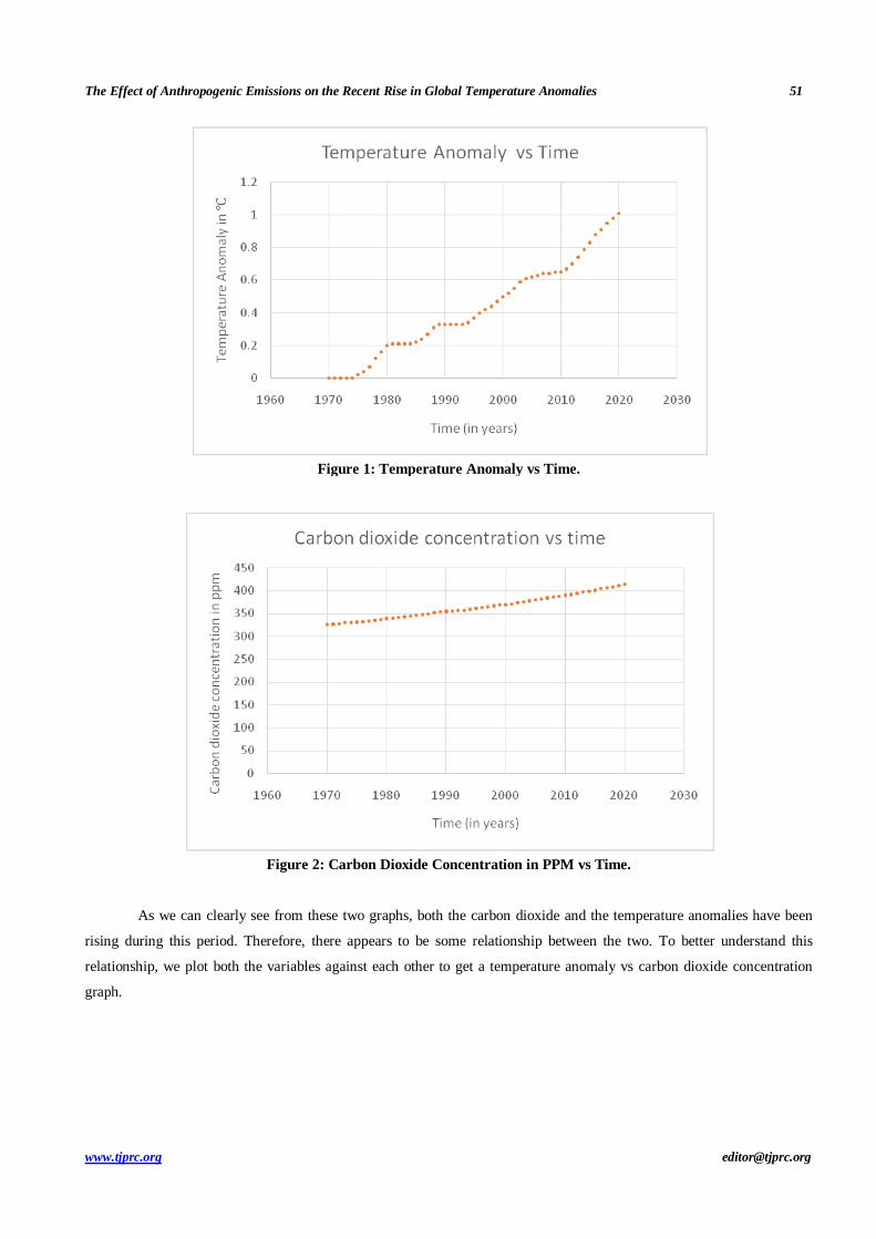
Figure 1: Temperature Anomaly vs Time.

Figure 2: Carbon Dioxide Concentration in PPM vs Time.

As we can clearly see from these two graphs, both the carbon dioxide and the temperature anomalies have been

rising during this period. Therefore, there appears to be some relationship between the two. To better understand this

relationship, we plot both the variables against each other to get a temperature anomaly vs carbon dioxide concentration

graph.

52 Sarva Sanjay


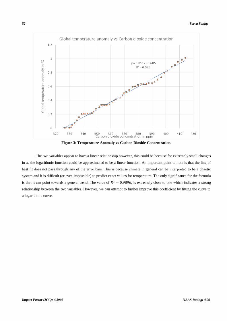
Figure 3: Temperature Anomaly vs Carbon Dioxide Concentration.

The two variables appear to have a linear relationship however, this could be because for extremely small changes

in 𝑥, the logarithmic function could be approximated to be a linear function. An important point to note is that the line of

best fit does not pass through any of the error bars. This is because climate in general can be interpreted to be a chaotic

system and it is difficult (or even impossible) to predict exact values for temperature. The only significance for the formula

is that it can point towards a general trend. The value of 𝑅2 = 0.9896, is extremely close to one which indicates a strong

relationship between the two variables. However, we can attempt to further improve this coefficient by fitting the curve to

a logarithmic curve.



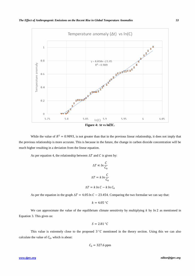
Figure 4: Δt vs lnC.

While the value of 𝑅2 = 0.9893, is not greater than that in the previous linear relationship, it does not imply that

the previous relationship is more accurate. This is because in the future, the change in carbon dioxide concentration will be

much higher resulting in a deviation from the linear equation.

As per equation 4, the relationship between Δ𝑇 and 𝐶 is given by:

Δ𝑇 ∝ 𝑙𝑛𝐶

𝐶0

Δ𝑇 = 𝑘 𝑙𝑛𝐶

𝐶0

Δ𝑇 = 𝑘 𝑙𝑛 𝐶 − 𝑘 𝑙𝑛 𝐶0

As per the equation in the graph Δ𝑇 = 4.05 𝑙𝑛 𝐶 − 23.454. Comparing the two formulae we can say that:

𝑘 = 4.05 °𝐶

We can approximate the value of the equilibrium climate sensitivity by multiplying 𝑘 by 𝑙𝑛 2 as mentioned in

Equation 3. This gives us:

𝑆 = 2.81 °𝐶

This value is extremely close to the proposed 3 °𝐶 mentioned in the theory section. Using this we can also

calculate the value of 𝐶0, which is about:

𝐶0 = 327.6 ppm

54 Sarva Sanjay


This is exactly the carbon dioxide concentration in the year 1972. Hence the data observed trend in temperature

anomalies matches that predicted by our model.

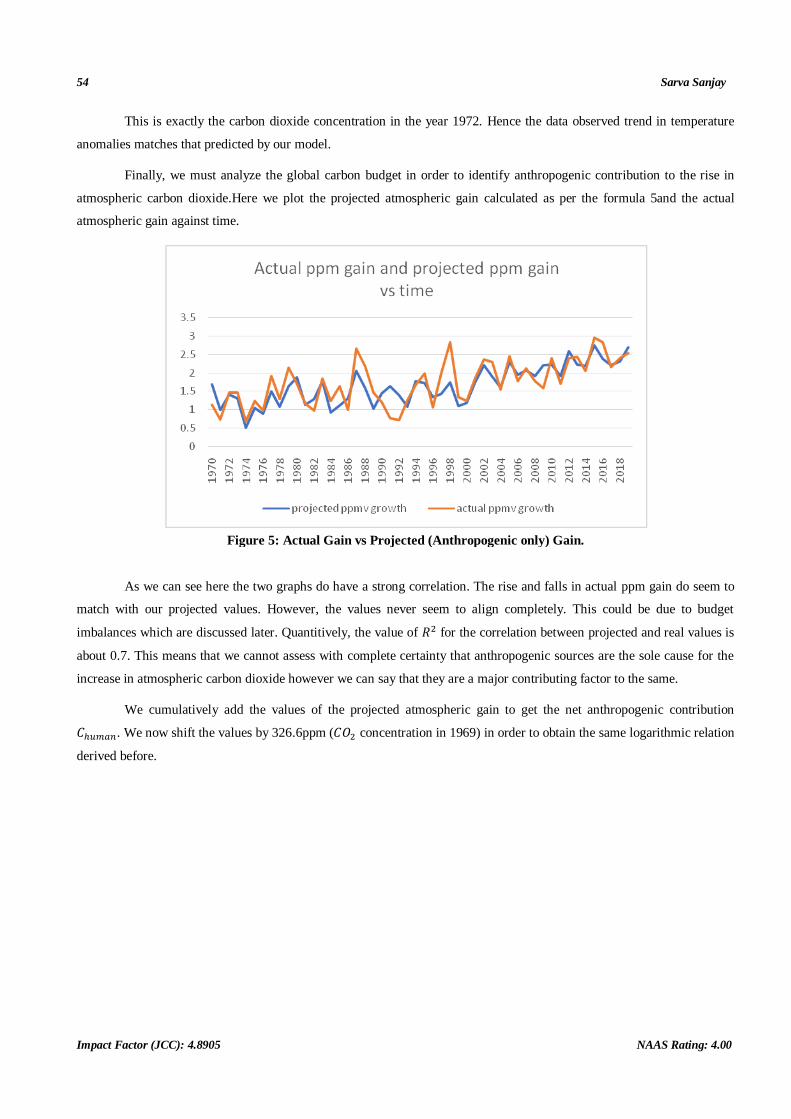
Finally, we must analyze the global carbon budget in order to identify anthropogenic contribution to the rise in

atmospheric carbon dioxide.Here we plot the projected atmospheric gain calculated as per the formula 5and the actual

atmospheric gain against time.

Figure 5: Actual Gain vs Projected (Anthropogenic only) Gain.

As we can see here the two graphs do have a strong correlation. The rise and falls in actual ppm gain do seem to

match with our projected values. However, the values never seem to align completely. This could be due to budget

imbalances which are discussed later. Quantitively, the value of 𝑅2 for the correlation between projected and real values is

about 0.7. This means that we cannot assess with complete certainty that anthropogenic sources are the sole cause for the

increase in atmospheric carbon dioxide however we can say that they are a major contributing factor to the same.

We cumulatively add the values of the projected atmospheric gain to get the net anthropogenic contribution

𝐶ℎ𝑢𝑚𝑎𝑛. We now shift the values by 326.6ppm (𝐶𝑂2 concentration in 1969) in order to obtain the same logarithmic relation

derived before.



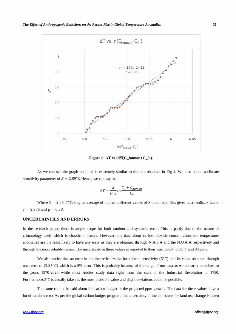
Figure 6: ΔT vs ln(C_human+C_0 ).

As we can see the graph obtained is extremely similar to the one obtained in Fig 4. We also obtain a climate

sensitivity parameter of 𝑆 = 2.89°𝐶.Hence, we can say that

Δ𝑇 =𝑆

𝑙𝑛 2𝑙𝑛

𝐶0 + 𝐶ℎ𝑢𝑚𝑎𝑛

𝐶0

Where 𝑆 = 2.85°𝐶(Taking an average of the two different values of S obtained). This gives us a feedback factor

𝑓 = 2.375 and 𝑔 = 0.58.

UNCERTAINTIES AND ERRORS

In the research paper, there is ample scope for both random and systemic error. This is partly due to the nature of

climatology itself which is chaotic in nature. However, the data about carbon dioxide concentration and temperature

anomalies are the least likely to have any error as they are obtained through N.A.S.A and the N.O.A.A respectively and

through the most reliable means. The uncertainty in these values is reported to their least count, 0.01°𝐶 and 0.1ppm.

We also notice that an error in the theoretical value for climate sensitivity (3°𝐶) and its value obtained through

our research (2.85°𝐶) which is a 5% error. This is probably because of the range of our data as we constrict ourselves to

the years 1970-2020 while most studies study data right from the start of the Industrial Revolution in 1750.

Furthermore,3°𝐶 is usually taken as the most probable value and slight deviations could be possible.

The same cannot be said about the carbon budget or the projected ppm growth. The data for these values have a

lot of random error.As per the global carbon budget program, the uncertainty in the emissions for land use change is taken

56 Sarva Sanjay


as 0.7 GtCyr-1, for ocean sink as 0.4GtCyr-1, for land sink as 0.9GtCyr-1 and for fossil fuel emissions at about 5%

percentage uncertainty. The uncertainty in cement carbonation is neglected as its value is too small (reported in megatons

carbon per year instead of gigatons carbon per year). Taking average of all uncertainties for fossil fuel emissions brings it

to an uncertainty of about 0.12 GtCyr-1. Using the formulae for uncertainty we can say that uncertainty in projected

atmospheric growth to be about 2.12 GtCyr-1 or 1.00ppm. This error is extremely high and, in some cases, even greater

than 100%. The reason behind this error is that the global carbon budget takes an average of several datasets each of which

have varying values. This error could be reduced by selecting one of those datasets, but this would make it susceptible to

systemic errors in the process of measurement. The error in the actual atmospheric gain is 0.1ppm which is reported to its

least count5.

The carbon budget also does not incorporate certain data which leads to a budget imbalance. For example, it does

not consider the anthropogenic contribution of 𝐶𝑂 and 𝐶𝐻4 in the carbon budget. They assume that all carbon monoxide

emissions arising from fossil fuel burning eventually convert into carbon dioxide and hence must not be double counted.

The anthropogenic emission of methane is not included in 𝐸𝐹𝑂𝑆 because fugitive emissions are not included in fuel

inventories. They eventually contribute to the carbon dioxide emission however their impact is assumed to be negligible.

Other anthropogenic changes in the sources of CO and CH4 from wildfires, vegetation biomass, wetlands, ruminants, or

permafrost changes are similarly assumed to have a small effect on the CO2 growth rate.Similarly, the contribution of

carbonates other than those from cement is also ignored.The missing processes include CO2 emissions associated with the

calcination of lime and limestone outside cement production. Finally a loss of sink capacity by the land due to the

replacement of from vegetation types that can provide a large carbon sink per area unit (typically, forests) to others less

efficient in removing CO2 from the atmosphere (typically, croplands) is also not included.

The main reason for the imbalance in the carbon budget is most likely the errors in 𝑆𝐿𝐴𝑁𝐷 and 𝑆𝑂𝐶𝐸𝐴𝑁. For

example, underestimation of the SLAND by DGVMs was reported following the eruption of Mount Pinatubo in 1991 which

caused the emission of sulphur aerosols into the sky which in turn caused diffused radiation which increased

photosynthetic activity thus enhancing the land sink13. Similar such examples have also been reported.

CONCLUSIONS

Despite the various sources of uncertainty and errors, we are able to assess the following details. Firstly, global

temperature anomaly is directly proportional to the natural log of the carbon dioxide concentration divided by the initial

concentration with an overall climate sensitivity estimated at about 3°𝐶. Second, we can say that most, if not all, of the

recent rise in carbon dioxide concentration are a result of anthropogenic activity. Using this we may conclude that the net

anthropogenic contribution to the gain in atmospheric carbon dioxide is the direct cause behind the rising global

temperature anomalies and that there exists a logarithmic relation between the two.

REFERENCES

1. Jacob, Daniel. Introduction to Atmospheric Chemistry. Illustrated, Princeton University Press, 1999.

2. Chamberlain, Joseph, and Donald Hunten. Theory of Planetary Atmospheres, Volume 36, Second Edition: An Introduction to

Their Physics and Chemistry (International Geophysics). 2nd ed., Academic Press, 1989.

13 Mercado, Lina M., et al. "Impact of changes in diffuse radiation on the global land carbon sink." Nature 458.7241 (2009): 1014-1017.



3. Lenton, Timothy M. “Land and Ocean Carbon Cycle Feedback Effects on Global Warming in a Simple Earth System Model.”

Tellus B, vol. 52, no. 5, 2000, pp. 1159–88. Crossref, doi:10.1034/j.1600-0889.2000.01104.x.

4. Myhre, Gunnar, et al. “New Estimates of Radiative Forcing Due to Well Mixed Greenhouse Gases.” Geophysical Research

Letters, vol. 25, no. 14, 1998, pp. 2715–18. Crossref, doi:10.1029/98gl01908.

5. Knutti, Reto, and Gabriele C. Hegerl. “The Equilibrium Sensitivity of the Earth’s Temperature to Radiation Changes.” Nature

Geoscience, vol. 1, no. 11, 2008, pp. 735–43. Crossref, doi:10.1038/ngeo337.

6. Hansen, J., et al. "Climate sensitivity: Analysis of feedback mechanisms." feedback 1 (1984): 1-3.

7. Tomassini, Lorenzo, et al. “Robust Bayesian Uncertainty Analysis of Climate System Properties Using Markov Chain Monte

Carlo Methods.” Journal of Climate, vol. 20, no. 7, 2007, pp. 1239–54. Crossref, doi:10.1175/jcli4064.1.

8. Friedlingstein, Pierre, et al. “Global Carbon Budget 2020.” Earth System Science Data, vol. 12, no. 4, 2020, pp. 3269–340.

Crossref, doi:10.5194/essd-12-3269-2020.

9. Change, Nasa Global Climate. “Global Surface Temperature | NASA Global Climate Change.” Climate Change: Vital Signs

of the Planet, climate.nasa.gov/vital-signs/global-temperature. Accessed 9 Apr. 2021.

10. Chylek, Petr, et al. “Limits on Climate Sensitivity Derived from Recent Satellite and Surface Observations.” Journal of

Geophysical Research, vol. 112, no. D24, 2007. Crossref, doi:10.1029/2007jd008740.

11. “Global Monitoring Laboratory - Carbon Cycle Greenhouse Gases.” The Global Monitoring Laboratory (GML) of the

National Oceanic and Atmospheric Administration, gml.noaa.gov/ccgg/trends/data.html. Accessed 9 Apr. 2021.

12. “---.” The Global Monitoring Laboratory (GML) of the National Oceanic and Atmospheric Administration,

gml.noaa.gov/ccgg/trends/gr.html. Accessed 9 Apr. 2021.

13. Mercado, Lina M., et al. "Impact of changes in diffuse radiation on the global land carbon sink." Nature 458.7241 (2009):

1014-1017.

14. Sarkar, Angshuman, Geethanjali Ravindran, and Vishnuvardhan Krishnamurthy. "A brief review on the effect of cadmium

toxicity: from cellular to organ level." Int J Biotechnol Res 3.1 (2013): 17-36.

15. Kashyap, Rachit, and K. S. Verma. "Seasonal variation of certain heavy metals in Kuntbhyog lake of Himachal Pradesh,

India." J Environ Ecol Fam Urb Stud 1.1 (2015): 15-26.

16. Srikanth, P., et al. "Analysis of heavy metals by using atomic absorption spectroscopy from the samples taken around

Visakhapatnam." International Journal of Environment, Ecology, Family and Urban Studies 3.1 (2013): 127-132.

17. Husain, Mohammed A. "An analysis of the Constraints of Policy Framework for Physical Planning in a Changing Climate in

Nigeria." International Journal of Environment, Ecology, Family and Urban Studies (IJEEFUS) ISSN (P) (2014): 2250-0065.

Documents

THE EFFECT OF ANTHROPOGENIC EMISSIONS ON THE …