THE EFFECT OF INTERNAL VARIABILITY ON ANTHROPOGENIC

THE EFFECT OF INTERNAL VARIABILITY ON ANTHROPOGENIC CLIMATE PROJECTIONS

Asgeir Sorteberg

Bjerknes Centre for Climate Research, University of Bergen, Norway

Nils Gunnar Kvamstø

Geophysical Institute, University of Bergen, Norway

Abstract An ensemble of climate change simulations is presented, with special emphasis on the spread among the different member. Using a single model ensemble, the spread in the climate change estimates may be interpreted as the effect of internal variability. As expected, the areas of significant changes increased with the strength of the CO2 forcing. For temperature this change was rapid in the absence of other external forcings 90% of the global area showed a significant change in 20-year averaged annual temperature around year 30. The global fraction for precipitation at the same time was around 30% which increased to 60% around doubling of CO2. The reduction of the spread by averaging over a longer period was investigated. An increase in averaging period from 15 to 30 years reduced the annual and seasonal grid point temperature spread by around 20% in most areas. The impact on the precipitation spread was about two third of that. This might provide some information on the design (resolution versus length of time period) of regional climate simulations. Analysis on the number of ensemble members needed to sample internal variability indicate that to require the same level of certainty for a Arctic temperature change as a tropical or subtropical the number of ensemble members should be increased by a factor of 5 to 6.

INTRODUCTION

Simulation of future climate change encompasses a wide range of uncertainties. Some are related to uncertainties in future external forcings like solar variability and emission of greenhouse gases and particles, while other are related to our understanding of the climate system and uncertainties due to internal climate variability. Thus, the spread among model results may both be due to real intermodel differences (parameterisations, level of sophistication, resolution), but also due to insufficient sampling of the natural internal variability of the climate system, which will add ‘noise’ to the climate signal imposed by changes in the external forcings. As computer capacity has increased the use of multiple realizations for more reliable estimates of the anthropogenic influence on future climate has become more common. These ensembles are either produced by a number of different models or a single model with perturbed model physics or perturbed initial conditions.

In this study we attempt to quantify the uncertainties related to insufficient sampling of internal variability using a single model with perturbed initial conditions. This uncertainty is depending on several factors. The length of the temporal averaging (averaging the results over a longer time period will smooth out natural variability), and

the spatial averaging (averaging over a larger area may reduce the natural variability). Thus we expect zonal means to be less influenced by natural variability than gridpoint values. In addition the strength of the external forcing and how strongly the external forcing is acting on the chosen meteorological parameter is important (eg. a stronger CO2 increase will reduce the relative influence of the natural variability on the result and natural variability may be more important for meteorological parameters that is less affected my increased CO2). As the amount of spatial or geographical averaging increases we expect the climate signal to be better defined, however this is on the expense of the geographical and temporal information content of the simulations. In this paper we do not cover the effect of spatial averaging on the signal and noise, but focus on the effect of temporal averaging and the strength of the external forcing. We believe an investigation into the changes in signal and noise behaviour might provide insight into how to best design global and regional climate change simulations and aid choices regarding the question of the number of ensemble members versus the complexity and therefore computationally cost of running the model.

The methodology and experimental setup is given in section 2. Section 3 discusses the changes in the models signal and noise with temporal averaging and strength of the external forcing while section 4 discusses the implication of this for the number of ensemble members needed to significantly detect a climate change. Section 5 discusses the single model spread (which represents natural variability) versus the multimodel spread (which represents both natural variability and real model differences).

METHODOLOGY AND EXPERIMENTAL SETUP An ensemble (consisting of 5 members) of CMIP2 (1% increase in CO2 per year) simulation with the coupled Bergen Climate Model (BCM) (Furevik et al., 2004) has been performed. The Bergen BCM consists of the atmospheric model ARPEGE/IFS together with a global version of the ocean model MICOM (including a dynamic-thermodynamic sea-ice model. The coupling between the two models is done with the software package OASIS. The atmosphere model has a linear TL63 (2.8°) resolution with 31 vertical levels. MICOM has an approximately 2.4° resolution with 24 isopycnal vertical levels. Key quantities regarding climatic means and variability of the control integration have been evaluated against available observations in Furevik et al. (2004). Evaluation of the variability and the stability of AMOC and other oceanic variability in the BCM and in the ocean only model run with daily forcing from NCEP/NCAR reanalysis (Kalnay et.al., 1996) has been investigated in a series of papers (Bentsen et al., 2002; Gao et al., 2003; Nilsen et al., 2003; Dutay et al., 2002). In general the model's Atlantic Meridional Overturning Circulation (AMOC) strength and variability is realistic with the AMOC being among the less sensitive to both a CO2 increase (10-15% AMOC reduction at doubling of CO2) and to freshwater perturbations (Otterå et al., 2003; 2004a; 2004b). The initial conditions for the CMIP2 members have been taken from 300-year control integration (Figure 1). The true state of the AMOC, which is a good measure of the poleward oceanic heat transport, is not exactly known and each experiment has been

initialized in different phases of the AMOC to span the natural variability (maximum difference in AMOC initial state between the different members was around 3 Sverdrups) of the AMOC. The simulations are integrated for 80 years until doubling of CO2 is reached. By systematically choose different initial states of the ocean heat transport we ensure that the spread among the different members are not underestimated as might be the case if only the atmospheric state is perturbed. Results indicate that the AMOC has a ‘memory’ of one to two decades (Collins et al., 2005), thus the initial state of the AMOC is assumed to directly influence the simulation during the first few decades. However, the initial state may have indirect effects on the simulations for a longer time since it might affect the initiation or enhance/reduce the strength of other feedbacks in the system.

Figure 1: The AMOC of the control simulation and the start of the five CMIP2 members.

ANALYSIS METHODS In a linear framework the temperature of the control and climate change simulation at a certain time may written as a function of the unperturbed mean control integration ( cntrlT ), plus a deterministic anthropogenic signal ( fT ) and internal variability under the

control ( 'cntrlT ) and climate change scenario ( '

2cmipT ), respectively '

cntrlcntrlcntrl TTT += (1) '

22 cmipfcntrlcmip TTTT ++= (2) Thus, difference in temperature between the control and climate change simulation at a certain time can be represented as:

( ) ( )''22 cntrlcmipfcntrlcmip TTTTTT −+=−=∆ (3)

For an ensemble of simulations fT is the deterministic (anthropogenic) signal which we

want to detect and give a certain confidence, while ( )''2 cntrlcmip TT − represent the random

(internal variability) component of the simulated climate change for a certain time period. The ensemble mean temperature change ({ }T∆ ) may then be written as: { } ( ){ }''

2 cntrlcmipf TTTT −+=∆ (4)

where { } indicates averaging over the ensemble members. We assume that the { }T∆ estimate from the n number of ensemble members is an unbiased estimate of the models ‘true’{ }T∆ , that the ensemble members are independent and that there is no covariability between the forced component and the temperature change variability. Thus, an unbiased estimate of the variance of the ensemble means change ( 2

T∆σ ) is:

{ }( ) ( ) ( ){ }[ ]11

1

2''2

''21

2

2

−−−−

=−

∆−∆= �� ==

∆ n

TTTT

n

TTn

i cntrlcmipcntrlcmip

n

iTσ (5)

which has a uncertainty that can be estimated using the chi-square relationship between the estimated variance of the ensemble mean change ( 2

T∆σ ) and the true variance ( 2

,TRUET∆σ ) :

2)2/1(

22

,22/

2 )1()1(

αα χσσ

χσ

−

∆∆

∆ −<<

− TTRUET

T nn (6)

where 2

2/αχ and 2)2/1( αχ − are properties of the chi-square distribution.

As the variance ( 2T∆σ ) only depend on the internal variability of the control and climate

change simulation, this is a measure of the climatic noise. From the above expression it is clear that the natural variability noise is a function of the spatial and temporal averaging of both the control and climate change simulations. In this paper the climate change ( T∆ ) is calculated as the difference between the temperature in the climate change simulation for a given time period and the mean temperature of the control integration over the 80 years of the climate change simulation. Thus, ''

cmipcntrl TT < and the variance of the

ensemble mean change ( 2T∆σ ) should be interpreted mainly as variance related to natural

variability within the climate change simulations. The signal-to-noise ratio is given as the absolute value of the ratio of the ensemble mean change over the standard deviation of the ensemble mean change:

{ }��

��

� ∆=∆T

Tabs

NS

σ (7)

Assuming that the temperature changes of the ensemble members are normal distributed, we may calculate the 100(1-�) % confidence interval for the true ensemble mean change given a infinite number of ensemble members ({ }TRUET∆ ) using the Student’s t-test:

{ } { } { }n

tTTn

tT TTRUE

T ∆∆ +∆<∆<−∆σσ

αα 2/2/ (8)

where 2/αt is a property of the t-distribution. Rearranging the above equation gives an estimate of the number of ensemble members required to calculate the climate change within a certain threshold ( E± ):

22/ �

�

��

�= ∆

Et

n Tσα (9)

THE BCM ENSEMBLES MEAN RESPONSE AND SIGNAL-TO-NOISE RATIO

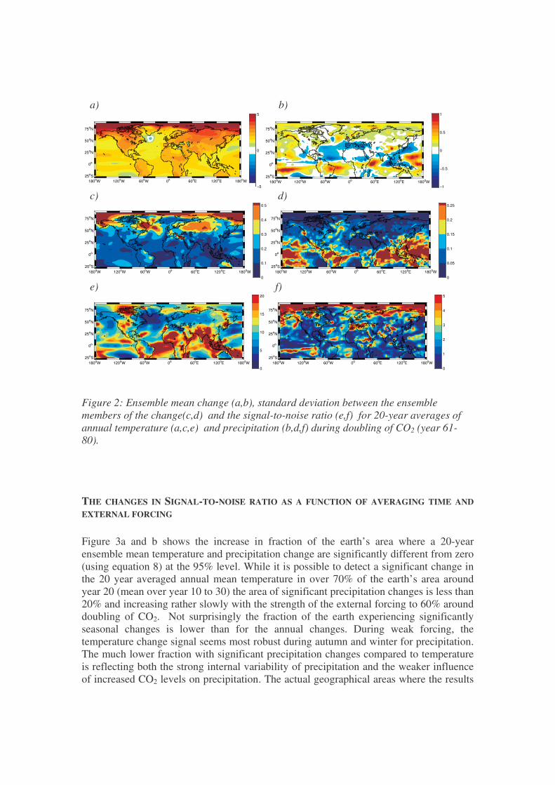
It seems fair to assume that the relative effect of natural variability on the climate change results will decline with the strength of the external forcing and to the extent the changes in external forcing influence the weather parameter we are interested in. Thus, in our 1% CO2 increase per year simulations, we expect the signal-to-noise ratio to increase with time during the integrations and be higher for weather parameters which is more strongly influenced by the changes in external forcing. Figure 2a and b shows the ensemble mean BCM annual temperature and precipitation change (equation 4), the standard deviation among the different members (equation 5) and the signal-to-noise ratio (equation 7) based on averages over year 60-80 when the external forcing it is relatively strong (a doubling of CO2). As with many other coupled models the BCM has a temperature change signature showing an Arctic climate change amplification (Figure 2a) and a particularly pronounced amplification over the Arctic ocean due to reduction of the sea ice. This is also the area showing the largest spread among the ensemble members (Figure 2c). Hence, in contrast to popular belief, even though the Arctic may have a large sensitivity to anthropogenic greenhouse gas changes its large internal variability does make it hard to attribute any climate variability to a particular external cause. The BCM simulations indicate part of the tropics as having the largest signal-to-noise ratio for temperature and therefore (given a case with a globally equal distribution of observations) the place where one easiest could attribute a climate change to human influence (Figure 2e). The picture is different for precipitation where the strongest changes are in the tropical areas, with a fairly pronounced intensification of the wintertime Hadley cell circulation (Figure 2f). In the tropics the spread among the different members (Figure 2d) follows the amplitude of the mean change. Surprisingly, the Arctic is the area of the largest signal-to-noise ratio for precipitation (Figure 2f). However, the signal-to-noise ratio is generally smaller than for temperature woldwide.

a) b)

−5

0

5

180oW 120oW 60oW 0o 60oE 120oE 180oW 25oS

0o

25oN

50oN

75oN

−1

−0.5

0

0.5

1


0o

25oN

50oN

75oN

c) d)

0

0.1

0.2

0.3

0.4

0.5


0o

25oN

50oN

75oN

0

0.05

0.1

0.15

0.2

0.25


0o

25oN

50oN

75oN

e) f)

0

5

10

15

20


0o

25oN

50oN

75oN

0

1

2

3

4

5


0o

25oN

50oN

75oN

Figure 2: Ensemble mean change (a,b), standard deviation between the ensemble members of the change(c,d) and the signal-to-noise ratio (e,f) for 20-year averages of annual temperature (a,c,e) and precipitation (b,d,f) during doubling of CO2 (year 61-80).

THE CHANGES IN SIGNAL-TO-NOISE RATIO AS A FUNCTION OF AVERAGING TIME AND EXTERNAL FORCING Figure 3a and b shows the increase in fraction of the earth’s area where a 20-year ensemble mean temperature and precipitation change are significantly different from zero (using equation 8) at the 95% level. While it is possible to detect a significant change in the 20 year averaged annual mean temperature in over 70% of the earth’s area around year 20 (mean over year 10 to 30) the area of significant precipitation changes is less than 20% and increasing rather slowly with the strength of the external forcing to 60% around doubling of CO2. Not surprisingly the fraction of the earth experiencing significantly seasonal changes is lower than for the annual changes. During weak forcing, the temperature change signal seems most robust during autumn and winter for precipitation. The much lower fraction with significant precipitation changes compared to temperature is reflecting both the strong internal variability of precipitation and the weaker influence of increased CO2 levels on precipitation. The actual geographical areas where the results

show statistical significant changes around doubling of CO2 is given by the areas having a signal-to-noise ratio above 2 in Figure 2e,f. a.) b.)

10 20 30 40 50 60 700

10

20

30

40

50

60

70

80

90

100

CENTER YEAR FOR 20 YEAR AVERAGES

FRA

CT

ION

OF

EA

RT

H (%

)

ANNUALDJFMAMJJASON

10 20 30 40 50 60 700

10

20

30

40

50

60

70

80

90

100

CENTER YEAR FOR 20 YEAR AVERAGES

FRA

CT

ION

OF

EA

RT

H (%

)

ANNUALDJFMAMJJASON

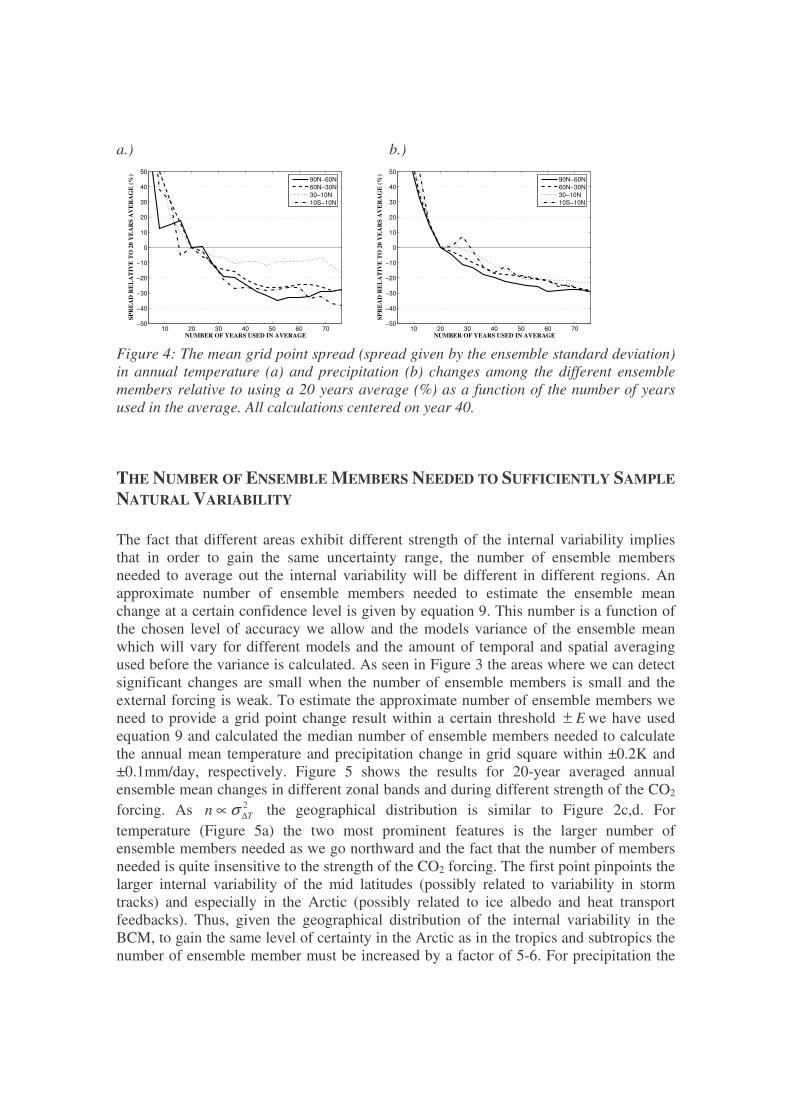
Figure 3: Fraction of global area witch have a 95% significant change in the 20-year averaged ensemble mean of temperature (a) and precipitation (b) as a function of simulation time (ie. The strength of the external forcing). As computer power still is a limiting factor when climate simulations are performed, there is a trade-off between the complexity and resolution of the model and the simulation length. Most regional downscaling simulations are performed over time slices of 15-30 years (IPCC, 2001), an important quantity is therefore how much the noise due to internal variability can be reduced when the length of the simulation is increased and the result can be averaged over a longer time period. Figure 4 shows the gain in increasing the averaging period relative to using a 20-year period. The changes were calculated by comparing the mean grid point spread among the different ensemble members (given by the ensemble standard deviation (equation 5) in selected zonal bands when different number of years is used in the averaging. All averages are centered on year 40 (e.g. If number of years used in averages is 10 the mean is the average from year 35 to 45. If the number of years are 20 it’s the average from year 30 to 50 etc.). For annual temperatures the spread for the 30-year average is reduced with around 20% in the Arctic, mid-latitude and tropical area and 10% for the subtropical area compared to the 20 year average, while for averaging times beyond 40-50 years the spread remains fairly constant (Figure 4a). The gain in reducing the precipitation spread when increasing the number of years used in the averaging is less. A reduction of 20% is not reached before the number of years is increased from 20 to over 40 (Figure 4b).

a.) b.)

10 20 30 40 50 60 70−50

−40

−30

−20

−10

0

10

20

30

40

50

NUMBER OF YEARS USED IN AVERAGE

SPR

EA

D R

EL

AT

IVE

TO

20

YE

AR

S A

VE

RA

GE

(%)

90N−60N60N−30N30−10N10S−10N

10 20 30 40 50 60 70−50

−40

−30

−20

−10

0

10

20

30

40

50

NUMBER OF YEARS USED IN AVERAGE

SPR

EA

D R

EL

AT

IVE

TO

20

YE

AR

S A

VE

RA

GE

(%)

90N−60N60N−30N30−10N10S−10N

Figure 4: The mean grid point spread (spread given by the ensemble standard deviation) in annual temperature (a) and precipitation (b) changes among the different ensemble members relative to using a 20 years average (%) as a function of the number of years used in the average. All calculations centered on year 40.

THE NUMBER OF ENSEMBLE MEMBERS NEEDED TO SUFFICIENTLY SAMPLE NATURAL VARIABILITY The fact that different areas exhibit different strength of the internal variability implies that in order to gain the same uncertainty range, the number of ensemble members needed to average out the internal variability will be different in different regions. An approximate number of ensemble members needed to estimate the ensemble mean change at a certain confidence level is given by equation 9. This number is a function of the chosen level of accuracy we allow and the models variance of the ensemble mean which will vary for different models and the amount of temporal and spatial averaging used before the variance is calculated. As seen in Figure 3 the areas where we can detect significant changes are small when the number of ensemble members is small and the external forcing is weak. To estimate the approximate number of ensemble members we need to provide a grid point change result within a certain threshold E± we have used equation 9 and calculated the median number of ensemble members needed to calculate the annual mean temperature and precipitation change in grid square within ±0.2K and ±0.1mm/day, respectively. Figure 5 shows the results for 20-year averaged annual ensemble mean changes in different zonal bands and during different strength of the CO2 forcing. As 2

Tn ∆∝ σ the geographical distribution is similar to Figure 2c,d. For temperature (Figure 5a) the two most prominent features is the larger number of ensemble members needed as we go northward and the fact that the number of members needed is quite insensitive to the strength of the CO2 forcing. The first point pinpoints the larger internal variability of the mid latitudes (possibly related to variability in storm tracks) and especially in the Arctic (possibly related to ice albedo and heat transport feedbacks). Thus, given the geographical distribution of the internal variability in the BCM, to gain the same level of certainty in the Arctic as in the tropics and subtropics the number of ensemble member must be increased by a factor of 5-6. For precipitation the

result are reversed. The tropical areas have a much stronger internal variability and therefore require a larger number of ensemble members. Given the fact that we have only 5 members the uncertainty in the calculation of the ensemble variance and therefore the number of ensemble members needed are large and should only be interpreted as indicative values. Bearing in mind the uncertainties, the results indicate that the number of members needed is quite insensitive to the strength of the CO2 forcing. This is consistent with our linear framework, where the variance of the ensemble mean change is only a function of the internal variability (equation 5). In addition this indicates that the amplitude of the internal variability is not significantly changed by the increased CO2 forcing. For the Arctic this last point may be somewhat surprising. Intuitively, a reduced ice and snow extent should lead to a reduced strength of the ice and snow albedo feedbacks and therefore reduced the internal variability. To test this one of the members was continued until 10 times CO2 was reached. The results showed that the internal variability of the Arctic was gradually reduced. Thus, in the case of the Arctic areas, the argument that the CO2 forcing does not influence the internal variability probably only holds for a moderate increase in the CO2 forcing. Note the 2E dependence in the estimation of the ensemble numbers (equation 9), thus if the thresholds E was reduced with a factor 2 the number of ensemble member needed would increase by a factor 4. a.) b.)

0

5

10

15

20

25

30

35

NU

MB

ER

OF

EN

SEM

BL

E M

EM

BE

RS

10S−10N 10N−30N 30N−60N 60N−90N

AVG. YEAR 20−39

AVG. YEAR 40−59

AVG. YEAR 60−79

0

5

10

15

20

25

30

35

NU

MB

ER

OF

EN

SEM

BL

E M

EM

BE

RS

10S−10N 10N−30N 30N−60N 60N−90N

AVG. YEAR 20−39AVG. YEAR 40−59AVG. YEAR 60−79

Figure 5: Median number of ensemble members needed to 95% confidently detect a annual mean gridpoint change in temperature(left) within ±0.2K and precipitation (right) within ±0.1mm/day in different areas. The number of ensemble members needed are calculated based on 20-year averages, for a weak (black), medium (grey) and strong (white) CO2 forcing.

THE SINGLE MODEL ENSEMBLE SPREAD VERSUS A MULTIMODEL ENSEMBLE SPREAD

The spread in result among different models may both be due to real intermodel differences, but also due to insufficient sampling of the internal variability of the climate system. By investigating the spread of the one model ensemble to the spread of a multimodel ensemble running the same 1% per year CO2 increase scenario, we may get knowledge of how much of the multimodel spread that can be attributed to insufficient sampling of internal variability. Figure 6 provides the precipitation and temperature change for the 5 BCM members and for 15 other models averaged over year 20-39 and 60-79, weak and strong CO2 forcing, respectively. With the exception of the Arctic, the BCM simulations are generally lower than the multimodel ensemble mean when it comes to precipitation changes and fairly close to the mean for temperature.

ARCTIC (60-90ºN)

0 0.5 1 1.5 2 2.5 3 3.5 4 4.5−5

0

5

10

15

20

TEMPERATURE CHANGE (C)

PRE

CIP

ITA

ION

CH

AN

GE

(%)

BCMOTHER MODELSMEAN OTHER MODELS

0 0.5 1 1.5 2 2.5 3 3.5 4 4.5−5

0

5

10

15

20


PRE

CIP

ITA

ION

CH

AN

GE

(%)


MID LATITUDES (30-60ºN)

0 0.5 1 1.5 2 2.5 3 3.5 4 4.5−5

0

5

10

15

20


PRE

CIP

ITA

ION

CH

AN

GE

(%)


0 0.5 1 1.5 2 2.5 3 3.5 4 4.5−5

0

5

10

15

20


PRE

CIP

ITA

ION

CH

AN

GE

(%)


SUB-TROPICS (10-30ºN)

0 0.5 1 1.5 2 2.5 3 3.5 4 4.5−5

0

5

10

15

20


PRE

CIP

ITA

ION

CH

AN

GE

(%)


0 0.5 1 1.5 2 2.5 3 3.5 4 4.5−5

0

5

10

15

20


PRE

CIP

ITA

ION

CH

AN

GE

(%)


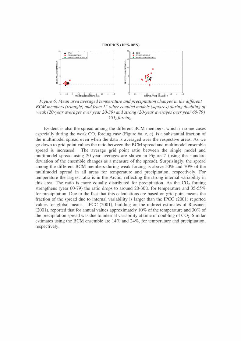
TROPICS (10ºS-10ºN)

0 0.5 1 1.5 2 2.5 3 3.5 4 4.5−5

0

5

10

15

20


PRE

CIP

ITA

ION

CH

AN

GE

(%)


0 0.5 1 1.5 2 2.5 3 3.5 4 4.5−5

0

5

10

15

20


PRE

CIP

ITA

ION

CH

AN

GE

(%)


Figure 6: Mean area averaged temperature and precipitation changes in the different

BCM members (triangle) and from 15 other coupled models (squares) during doubling of weak (20-year averages over year 20-39) and strong (20-year averages over year 60-79)

CO2 forcing.

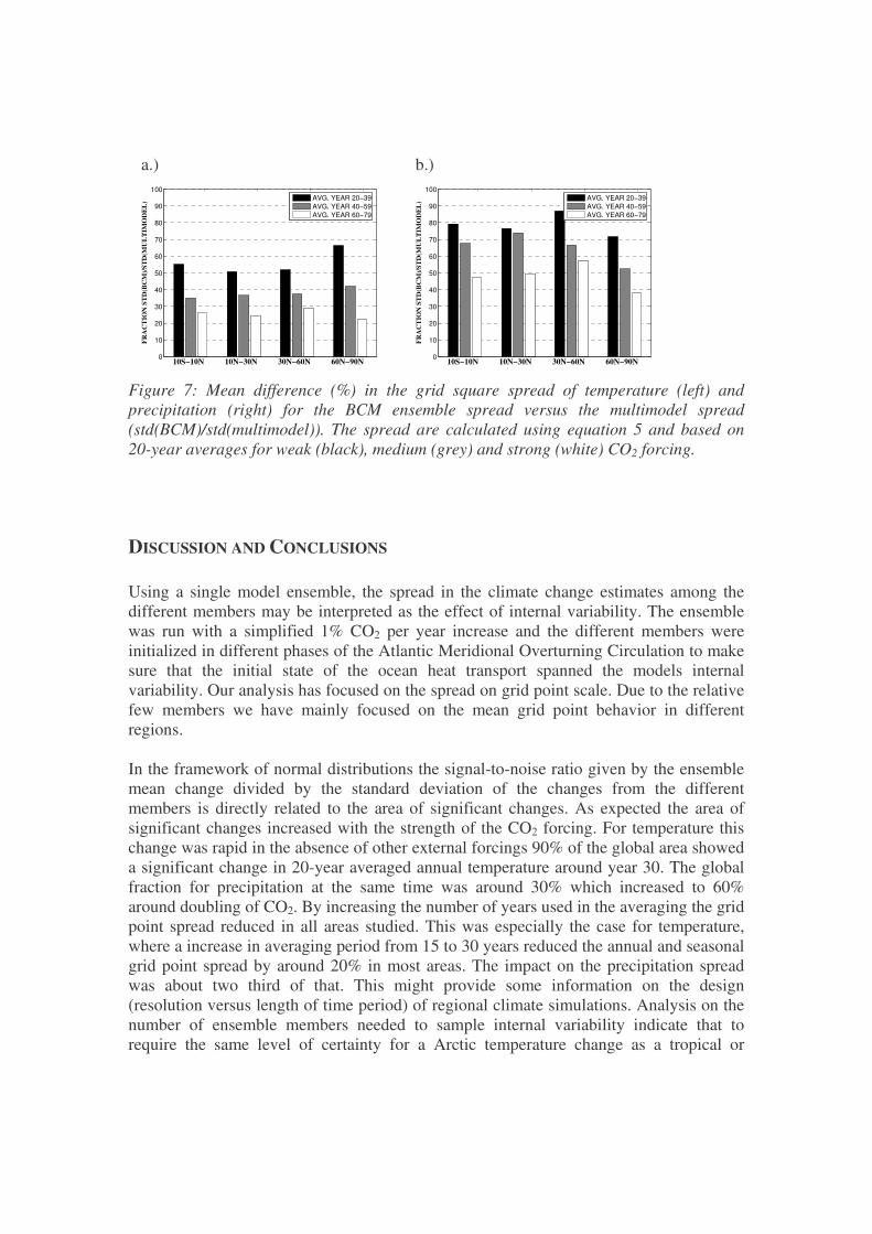
Evident is also the spread among the different BCM members, which in some cases especially during the weak CO2 forcing case (Figure 6a, c, e), is a substantial fraction of the multimodel spread even when the data is averaged over the respective areas. As we go down to grid point values the ratio between the BCM spread and multimodel ensemble spread is increased. The average grid point ratio between the single model and multimodel spread using 20-year averages are shown in Figure 7 (using the standard deviation of the ensemble changes as a measure of the spread). Surprisingly, the spread among the different BCM members during weak forcing is above 50% and 70% of the multimodel spread in all areas for temperature and precipitation, respectively. For temperature the largest ratio is in the Arctic, reflecting the strong internal variability in this area. The ratio is more equally distributed for precipitation. As the CO2 forcing strengthens (year 60-79) the ratio drops to around 20-30% for temperature and 35-55% for precipitation. Due to the fact that this calculations are based on grid point means the fraction of the spread due to internal variability is larger than the IPCC (2001) reported values for global means. IPCC (2001), building on the indirect estimates of Raisanen (2001), reported that for annual values approximately 10% of the temperature and 30% of the precipitation spread was due to internal variability at time of doubling of CO2. Similar estimates using the BCM ensemble are 14% and 24%, for temperature and precipitation, respectively.

a.) b.)

0

10

20

30

40

50

60

70

80

90

100

FRA

CT

ION

ST

D(B

CM

)/ST

D(M

UL

TIM

OD

EL

)

10S−10N 10N−30N 30N−60N 60N−90N


0

10

20

30

40

50

60

70

80

90

100

FRA

CT

ION

ST

D(B

CM

)/ST

D(M

UL

TIM

OD

EL

)

10S−10N 10N−30N 30N−60N 60N−90N


Figure 7: Mean difference (%) in the grid square spread of temperature (left) and precipitation (right) for the BCM ensemble spread versus the multimodel spread (std(BCM)/std(multimodel)). The spread are calculated using equation 5 and based on 20-year averages for weak (black), medium (grey) and strong (white) CO2 forcing.

DISCUSSION AND CONCLUSIONS Using a single model ensemble, the spread in the climate change estimates among the different members may be interpreted as the effect of internal variability. The ensemble was run with a simplified 1% CO2 per year increase and the different members were initialized in different phases of the Atlantic Meridional Overturning Circulation to make sure that the initial state of the ocean heat transport spanned the models internal variability. Our analysis has focused on the spread on grid point scale. Due to the relative few members we have mainly focused on the mean grid point behavior in different regions. In the framework of normal distributions the signal-to-noise ratio given by the ensemble mean change divided by the standard deviation of the changes from the different members is directly related to the area of significant changes. As expected the area of significant changes increased with the strength of the CO2 forcing. For temperature this change was rapid in the absence of other external forcings 90% of the global area showed a significant change in 20-year averaged annual temperature around year 30. The global fraction for precipitation at the same time was around 30% which increased to 60% around doubling of CO2. By increasing the number of years used in the averaging the grid point spread reduced in all areas studied. This was especially the case for temperature, where a increase in averaging period from 15 to 30 years reduced the annual and seasonal grid point spread by around 20% in most areas. The impact on the precipitation spread was about two third of that. This might provide some information on the design (resolution versus length of time period) of regional climate simulations. Analysis on the number of ensemble members needed to sample internal variability indicate that to require the same level of certainty for a Arctic temperature change as a tropical or

subtropical the number of ensemble members should be increased by a factor of 5 to 6 and vice versa for precipitation. REFERENCES Bentsen, M., H. Drange, T. Furevik and T. Zhou (2004), Variability of the Atlantic thermohaline circulation in an

isopycnic coordinate OGCM, Clim. Dynam. In Press Collins M., Botzet, A. Carril, H. Drange, A. Jouzeau, M. Latif, O.H. Otteraa, H. Pohlmann, A. Sorteberg, R. Sutton, L.

Terray (2005), Interannual to Decadal Climate Predictability: A Multi-Perfect-Model-Ensemble. J. of Climate, submitted.

Dutay, J.-C., J.L. Bullister, S.C. Doney, J.C. Orr, R. Najjar, K. Caldeira, J.-M. Champin, H. Drange, M. Follows, Y. Gao, N. Gruber, M.W. Hecht, A. Ishida, F. Joos, K. Lindsay, G. Madec, E. Maier-Reimer, J.C. Marshall, R.J. Matear, P. Monfray, G.-K. Plattner, J. Sarmiento, R. Schlitzer, R. Slater, I.J. Totterdell, M.-F. Weirig, Y. Yamanaka, and A. Yool (2002), Evaluation of ocean model ventilation with CFC-11: comparison of 13 global ocean models. Ocean Modelling, 4, 89-120

Furevik T., Bentsen, M., Drange, H., Kindem, I.K.T., Kvamstø, N.G., and Sorteberg, A. (2003): Description and Validation of the Bergen Climate Model: ARPEGE coupled with MICOM, Climate Dynamics, No. 21, pp. 27-51, 2003

Gao, Y., H. Drange and M. Bentsen (2003), Effects of diapycnal and isopycnal mixing on the ventilation of CFCs in the North Atlantic in an isopycnic coordinate OGCM, Tellus, 55B, 837-854.

IPCC, (2001): Climate Change 2001. The scientific basis. Eds. J. T. Houghton, Y. Ding, M. Nogua, D. Griggs, P. Vander Linden, K. Maskell, Cambridge Univ. Press., Cambridge, U.K.

Kalnay, E., M. Kanamitsu, R. Kistler, W. Collins, D. Deaven, L. Gandin, M. Iredell, S. Saha, G. White, J. Woolen, Y. Zhu, M. Chelliah, W. Ebisuzaki, W. Higgins, J. Janowiak, K. C. Mo, C. Ropelewski, J. Wang, A. Leetma, R. Reynolds, R. Jenne, and D. Joseph, 1996: The NCEP/NCAR 40-year reanalysis project. Bulletine of Amer. Meteorol. Soc., 77, 437-471.

Nilsen, J. E. Ø., Y. Gao, H. Drange, T. Furevik and M. Bentsen (2003): Simulated North Atlantic-Nordic Seas water mass exchanges in an isopycnic coordinate OGCM, Geophys. Res. Lett., 30, 1536

Otterå, O. H., H. Drange, M. Bentsen, N. G. Kvamstø and D. Jiang (2003): The sensitivity of the present day Atlantic meriodinal overturning circulation to anomalous freshwater input, Geophysical Research Letters, Vol. 30, No. 17, pp. 3-1-3-4.

Otterå, O. H. and H. Drange (2004a): A possible coupling between the Arctic fresh water, the Arctic sea ice cover and the North Atlantic Drift. A case study. Advances in Atmospheric Sciences, Vol. 21, No. 5, pp. 784-801.

Otterå, O. H. H. Drange, M. Bentsen, N. G. Kvamstø and D. Jiang (2004b): Transient response of enhanced freshwater to the Nordic Seas-Arctic Ocean in the Bergen Climate Model, Tellus, Vol. 56, pp. 342-361

Raisanen J. (2001). Co2-induced climate change in CMIP2 experiments. Quantification of agreement and role of internal variability. J. of Climate, 14, 2088-2104.

Documents

THE EFFECT OF INTERNAL VARIABILITY ON ANTHROPOGENIC