South Dakota State UniversityOpen PRAIRIE: Open Public Research Access InstitutionalRepository and Information Exchange

Department of Economics Staff Paper Series Economics

4-22-2014

The Effect of Biotechnology and Biofuels on U.S.Corn Belt Cropping Systems.Scott FaustiSouth Dakota State University

Evert Van der SluisSouth Dakota State University

Bahir QasmiSouth Dakota State University

Jonathan Lundgren

Follow this and additional works at: http://openprairie.sdstate.edu/econ_staffpaper

Part of the Agricultural and Resource Economics Commons

This Article is brought to you for free and open access by the Economics at Open PRAIRIE: Open Public Research Access Institutional Repository andInformation Exchange. It has been accepted for inclusion in Department of Economics Staff Paper Series by an authorized administrator of OpenPRAIRIE: Open Public Research Access Institutional Repository and Information Exchange. For more information, please contactmichael.biondo@sdstate.edu.

Recommended CitationFausti, Scott; Van der Sluis, Evert; Qasmi, Bahir; and Lundgren, Jonathan, "The Effect of Biotechnology and Biofuels on U.S. Corn BeltCropping Systems." (2014). Department of Economics Staff Paper Series. Paper 203.http://openprairie.sdstate.edu/econ_staffpaper/203

i

The Effect of Biotechnology and Biofuels

on U.S. Corn Belt Cropping Systems

by

Scott Fausti, Evert Van der Sluis, Bashir Qasmi and Jonathan Lundgren

Economics Staff Paper No. 2014-1 April 22, 2014

Papers in the SDSU Economics Staff Paper series are reproduced and distributed to encourage discussion of research, extension, teaching, and public policy issues. Although available to anyone on request, the papers are intended primarily for peers and policy makers. Papers are normally critiqued by some colleagues prior to publication in this series. However, they are not subject to the formal review requirements of South Dakota State University’s Agricultural Experiment Station and Extension Service publications. *Scott Fausti is a Professor of Economics; Evert Van der Sluis is a Professor of Economics; Bashir A. Qasmi is an Associate Professor; and Jonathan Lundgren is with the Agricultural Research Service in Brookings, SD. Contact Author: Scott Fausti, South Dakota State University, Department of Economics, Box 504 Scobey Hall, Brookings, SD (Ph 605-688-6848. E-mail scott.fausti@sdstate.edu

ii

The Effect of Biotechnology and Biofuels on U.S. Corn Belt Cropping Systems

Abstract

The effects of transgenic crop and federal biofuel policy on state-level cropping patterns in

the Corn Belt region are investigated (2000-2012). The literature links the expansion of corn

acreage to the supplanting of small grain and hay acreage in this region. Empirical evidence

generated by a random intercept model with fixed effects indicates that the intensification of

corn acres planted was positively impacted by biotech advancements in energy and

agriculture. This suggests producers are moving away from diverse cropping patterns and

the rotational practices associated with a diverse crop planting strategy. However, the

empirical evidence suggests that the effects of these biotech advancements on producer

planting decisions are heterogeneous across states. Thus, future policy changes affecting

producer corn production decisions will not be uniform across States.

1

The Effect of Biotechnology and Biofuels on U.S. Corn Belt Cropping Systems

1. Introduction:

An empirical investigation into the linkage between the usage of genetically-enhanced crops in

production agriculture, bioenergy produced from these crops, and their combined effects on cropping

patterns at the state level in the U.S. Corn Belt region is conducted based on annual data from 2000 to

2012. The United States experienced dramatic changes in row crop production practices during this

period, particularly in the Corn Belt region, as documented by, for example, Wallander et al. 2011.

The objective of this study is to identify how ethanol (ethyl alcohol) policy, relative corn (Maize)

to soybean (Glycine max) prices, and adoption rates of genetically modified (GM) corn affect corn

acreage intensity differences across States. Our findings suggest that the effects of changes in bioenergy

policy, relative crop prices, and the ability of GM technology to continue to provide pest protection

(Landis et al. 2008; Hutchison et al. 2010; Gassmann et al. 2011) on producer cropping decisions vary by

state across the Corn Belt region. Hence, future agricultural policy decisions need to recognize that

producer reaction to changes in the above factors will be depended on geographical location (Van der

Sluis et al. 2002).

We investigate the relationship between the rapid increase in the reliance on GM varieties in

corn production, the simultaneous upsurge in corn-based biofuel production and the associated

increase in the derived demand for corn on state-level corn acreage intensity. Our empirical results

suggest cropping patterns were affected by the rapid increase in ethanol production due to biofuel

policies, facilitated in part by the increased reliance on genetically-enhanced corn varieties, and the

increased profitability of growing corn relative to other crops. These factors have contributed

significantly to the increase in the proportion of corn acres planted in the U.S. Corn Belt region, but our

analysis shows that the effect on corn production intensity varies between states.

2

2. Linking GM Corn Production, Ethanol Production, and Corn Acreage Intensity

The evolution of agricultural practices in the eleven states of the Corn Belt region (IA, IL, IN, NE, KS, MI,

MN, MO, OH, SD, and WI) over the last quarter-century has resulted in a movement away from

conventional row crop production practices. These conventional cropping practices helped maintain soil

fertility (crop rotation effect) and reduce the damage associated with weed and insect pests that

negatively impact crop productivity. Today, the U.S. crop production system relies heavily on chemical

and genetic technology to maintain soil fertility and keep agricultural pests at bay. This transition has

been supported by changes in U.S. energy and agricultural policy decisions, and advancements in

biotechnology that, in turn, have fostered the growth of the ethanol and agricultural seed industries.

2.1 U.S. Agricultural and Energy Policies

The period between 1996 and 2012 has been identified in the literature as a transitional one in

American agriculture. During this period, row crop producers have moved away from conventional crop

rotation practices to a more crop-intensive production system, especially for corn and soybean

production (Wallander et al. 2011; Johnston 2014). Claassen et al. (2010), maintain that changes in U.S.

cropping decisions by producers were facilitated primarily by policy changes embodied in the 1996 Farm

Bill (P.L. 104-127), commonly referred to as the “Freedom to Farm Act” (FFA), which decoupled the

income support system for row crop producers and removed the set-aside requirements for support

payments (Mercier 2011). Claassen et al. (2010) assert that these policy changes allowed agricultural

producers to respond more directly to market signals, policy incentives, and changes in technology. The

latter include the use of GM crops, which enabled farmers to reduce labor requirements for crop

production during the planting season, as first documented by Fernandez-Cornejo and McBride (2002).

The development of corn and soybean-based biofuel conversion technology as alternatives to

fossil fuels allowed U.S. energy policy to include programs that require using minimal levels of biofuels

blended in with transportation fuels. The overall goal of these mandates is to have biofuels become an

3

important source of energy for the U.S. economy. The two primary legislative mandates are the 2005

Energy Policy Act and the Energy Independence and Security Act of 2007. The legislation sets minimum

annual consumption levels in four broad-based biofuel categories: cellulosic, biomass-based diesel,

undifferentiated-advanced, and renewable energy. The mandate for all biofuels in 2022 is set at 36

billion gallons. Currently, the corn-starch based ethanol production cap is set to reach 15 billion gallons

in 2015, and remain fixed going forward (Schnepf and Yacobucci 2013). However, corn-based ethanol is

by far the main source of biofuel production because of its cost advantage relative to alternative

biofuels. Given the current state of production technology for non-corn-starch based ethanol

alternatives, the 36 billion gallon ethanol mandate is unrealistic unless the 15 billion gallon cap is

removed from corn-starch based ethanol production.

2.2 Biofuel Commercialization

According to the Renewable Fuels Association (2014) the U.S. produced 175 million gallons of ethanol in

1980, 848 million gallons in 1990, and 1.622 billion gallons in 2000. In 2000, the U.S produced 9.97

billion bushels of corn which indicates that the ethanol industry consumed about 6.5 percent of the U.S.

corn crop that year. Thus, in the first 20 years of its existence, only a small percentage of the annual corn

crop flowed into the ethanol industry.

California’s decision to ban the use of MTBE (methyl tertiary-butyl ether) and use ethanol as a

gasoline additive substitute provided the initial increase in demand that fueled expansion of the ethanol

industry. Passage of the 2005 Energy Policy Act created a renewable fuel standards policy in the United

States that imposed ethanol mandates and spurred refiners nationwide to increase their demand for

ethanol as the U.S. made a rapid conversion from MTBE to ethanol (EPA, 2014).

Statistics provided by the Renewable Fuels Association (2014) indicate that 95 ethanol plants

produced 3.9 billion gallons in 2005. In the same year, the U.S. produced 11.1 billion bushels of corn.

The estimated share of the 2005 corn production consumed by the ethanol industry reached 12.9

4

percent in 2005.1 By the end of 2013, the number of ethanol plants in the United States had increased to

210, with a total capacity of 15 billion gallons, and a total production of 13.3 billion gallons per year. In

2013, the U.S. produced 13.9 billion bushels of corn. Using a FAPRI 2012 conversion rate of 2.77, the

ethanol industry consumed approximately 34 percent- of the 2013 corn crop. The corn-based ethanol

industry has grown from a minor to a major industry in less than 15 years (Cai and Stiegert 2014). This

rapid expansion contributed to corn price increases which, in turn, sent a positive market signal to row

crop producers to substantially increase their corn production. Changes in the agricultural production

policies due to the 1996 Freedom to Farm Act allowed producers to increasingly shift production

practices toward corn after corn, corn and soybean rotations, double cropping, and move away from

planting other conventional crops in a rotation. To accomplish this switch, producers made a rapid

transition from planting conventional to GM seed.

2.3 Commercialization of GM Seed Technology for Corn and Soybeans

GM crop varieties were first introduced for commercial production in the United States in 1996. Since

then, farmers have rapidly adopted herbicide tolerance (HT: glufosinate), insect resistance (Bt: Bacillus

thuringeiensis), and stacked (both traits) GM corn and soybean varieties. The U.S. adoption rates of GM

corn and soybeans increased from zero in 1995, to 25 percent and 54 percent in 2000, and to 90 percent

and 93 percent in 2013, respectively (Economic Research Service, 2014).

Numerous authors have noted the rapid adoption and diffusion of GM crops, and various

studies provide documentation of an array of implications of the increased reliance on GM crop varieties

(e.g. Benbrook 2004; Cattaneo et al. 2006, Benbrook 2009; Fernandez-Cornejo et al. 2014). In their

analysis of adoption and diffusion decisions and patterns, Scandizzo and Savastano (2010) suggest that

once farmers begin to adopt GM crops in their production systems, producers reach a point where it

becomes too costly to switch back to conventional crop varieties (pp.144-145). The authors provide

1 We used the Food and Agricultural Policy Research Institute (FAPRI) 2005 conversion rate of 2.71 gallons per

bushel to estimate corn production usage by the ethanol industry for 2005.

5

several reasons for why irreversibility may occur. They argue that producers find it difficult to return to

conventional crops because they have incomplete information about pest pressures at the time of

planting. Learning and experimenting with new technologies involves sunk costs. Adopting GM crops

requires making investments specific to the new technology (among other things, increased use of

larger scale specialized, and no-till equipment, etc.). The authors suggest that GM crop adoption and

diffusion may reduce biodiversity, enhance pest resistance, and cause irreversible biological effects due

to the spread of genes to non-target wild species (p.145). Thus, the irreversibility of the adoption of GM

crops and their high diffusion rates represent a dramatic change in the types of agriculture observed,

including the types of crops planted and cropping patterns.

The issue of the diffusion of GM crops linked to the intensification of the same crops extends

beyond the borders of the U.S. For example, Cap and Malach (2012) reported on changes in land use

patterns due to the increased area planted to soybeans in general, and the increased reliance on GM

soybeans in particular, in four South American nations. The authors found that the commercial

availability of glyphosate-tolerant soybean varieties contributed to an increase in the area planted to

soybeans in three of the four main South American soybean-producing nations.

2.4 Cropping Pattern over time

Corn Belt states have experienced a significant change in crop production patterns since the

passage of the FFA in 1996. In particular, these states experienced a major shift away from small grains,

wheat (Triticum), and hay, toward corn and soybeans (Table 1). According to Johnston (2014), Wallander

et al. (2011), and Claassen et al. (2010), the cropping system in the Corn Belt and Eastern Northern

Plains underwent substantial change since the mid-1990s. Johnston (2014) has documented the

conversion of grasslands in the Prairie Pothole Region (PPR) of the U.S. into corn-soybean acreage.

Johnston presents data indicating that this change in the cropping pattern has resulted in the

supplanting of wheat and other small grains in the PPR. Claassen et al. (2010) identifies a significant

6

conversion of marginal production acres (grasslands, hay-land) to cropland in the Eastern Northern

Plains. Wallander et al. (2011) note that the increase in the U.S. corn and soybean acreage over the past

decade has coincided with the increased incidence of double cropping, the conversion of hay land, and a

reduction in cotton (Gossypium hirsutum) acreage.

The extensive literature on changing cropland patterns has linked the emergence of corn-based

ethanol production to changes in cropping patterns in general. However, no econometric analyses have

been conducted on the role of federal ethanol policies, relative crop prices, and GM seed adoption in

state-level cropping patterns using a “mixed model” approach. Given the heterogeneous nature of

individual State climate and soil conditions, understanding the effects of policy and technology on state

cropping patterns must account for state-level characteristics. To capture the heterogeneity between

states, a mixed modeling approach that incorporates both random and fixed effects was adopted.

3. Data

Our analysis is based on secondary state‐level data on crop acres planted and GM corn coverage in

eleven northern Corn Belt states for each year between 2000 and 2012, resulting in a total of 143

observations. In particular, our data set includes state-level cropland acres planted for IA, IL, IN, NE, KS,

MI, MN, MO, OH, SD, and WI between 1996 and 2012, collected from the National Agricultural Statistics

Service (2014). We also collected annual GM crop adoption rates for the eleven northern Corn Belt

states from the Economic Research Service (2014) from 2000 to 2012 (genetically modified crop

adoption rates for years prior to 2000 were not available). A policy dummy variable was created based

on the passage of the 2005 Energy Policy Act and the Energy Independence and Security Act of 2007.

The dummy variable has a value of one for the years 2005 to 2012, zero otherwise. Annual average corn

and soybean prices were collected from the National Agricultural Statistics Service (2014).

7

4. Methodology

Given the nature of our state-level pooled time series/cross-sectional data set, we adopted a linear

mixed modeling approach to investigate the effect of GM corn adoption and the enactment of ethanol

policies on changes in state-level corn acreage intensity. Our objective is to investigate how corn

acreage planted as a proportion of total cropland acres planted in the eleven-state region has changed

during this transition period. We hypothesize that agricultural sector heterogeneity between states – for

example, differences in climate, soil, landscape, and state agricultural policies – has resulted in dissimilar

responses to the introduction of biotechnology and bioenergy policy during the transition period

covered in our study.

Using annual data, we apply a mixed regression modeling approach to estimate a fixed effects

model with a random intercept by state. Four models were estimated: a) no interaction terms (the

simple model), b) the GMCS/State interaction term model; c) the RFS/State interaction term model, and

d) the PR/State interaction term model. We hypothesize that data on acres planted are clustered due to

the heterogeneity of individual state characteristics.2 The dependent variable is the ratio of corn acres

planted to total acres planted, or corn acreage intensity (CAI) by state. Explanatory variables include the

ratio of annual corn to soybean prices (PR); an ethanol policy dummy variable (RFS=1 for years from

2005 to 2012); and the state‐level percentage of corn acres planted with GM corn seed (GMCS). We

assume each of these explanatory variables has a positive relationship with CAI. We also created fixed

effects interaction terms designed to identify the effect of GMCS adoption rates, RFS policy on state-

level CAI, and the effect of the change in the relative price of corn to soybeans on State level CAI.3 The

price ratio variables captures the market valuation of corn relative to other crops, the GMCS variable

2 Clustered data refer to attributes associated with an individual state’s agricultural sector, such as climate, soil

type, landscape, and state-level agricultural policies that would result in a clustering of similar cropping patterns between geographically related states. The existence of cluster data will result in biased standard errors. Clustering was verified and a correction procedure was implemented. 3 The fixed effects interaction terms for GMCS and PR represent individual state slope coefficients for the

explanatory variables.

8

reflects the supply side impact of biotechnology on corn production, and the RFS policy dummy variable

captures the increased demand for corn due to corn-based ethanol production policy incentives.

The standard assumptions associated with the linear mixed model (LML) are listed in equations

1-4. Using the standard vector notation provided on page 121 in the SAS/Stat 9.3 User Guide (SAS

Institute, 2011), we define the general structure of the model:

( )

( ) and

( )

The dependent variable CAI denotes the vector of dependent variable observations. Matrix X is

the design matrix associated with β, which represents the vector of unknown fixed effects parameters.

Matrix Z is the design matrix associated with ϒ, representing the vector of unknown random effects

parameters. The error term, ε, reflects an unknown random error. Equation 4 states that ϒ and ε are

independent, which implies that the variance of CAI (SAS Institute, 1999: p. 2087) can be defined as:

[ ] 4

G and R are the covariance matrices associated with ϒ and ε, respectively.5 The LML procedure in SAS

provides great flexibility when dealing with regression diagnostic issues (SAS Institute, 1999). First, we

employed a “sandwich estimator” approach to produce robust standard errors associated for β (SAS

Institute, 1999, chapter 41; and Diggle et al., 1994).

We estimated four models. The first model is a simple random intercept model containing fixed

effects for the PR, GMCS, and RFS variables. The second model is a random intercept model with a

4 The superscript notation “T” denotes the transpose matrix operation. We also examined the correlation

between the model’s residuals and the exogenous variables. All correlation coefficients were less than 0.01. Thus, exogeneity is confirmed. 5 The default covariance structure for the Mixed procedure is variance components (SAS 1999: p. 2088). Other

covariance structures for G and R were investigated. The variance components structure was selected based on the “Null Model Likelihood Ratio Test.”

9

GMCS interaction term, where the simple model is extended by adding a fixed effects interaction term

for State*GMCS.6 The interaction variable’s parameter estimate, δ, is a slope coefficient, reflecting for

the effect of each specific state’s GM corn adoption rate on the proportion of corn acres planted. The

third model is a random intercept model with the RFS interaction term, where the simple model is

extended by adding a fixed effects interaction term for state*RFS. The interaction variable’s parameter

estimate, δ, captures each individual state’s fixed effects intercept adjustment coefficient for the effect

of federal ethanol policy on the same state’s proportion of corn acres planted. The fourth model is a

random intercept model with the PR interaction term, where the simple model is extended by adding a

fixed effects interaction term for state*PR. The interaction variable’s parameter estimate, δ, captures

the state-specific fixed effects estimated slope coefficient for the effect of the change in the relative

price of corn to soybeans on corn acres planted.7 The linear form of the general model to be estimated

is:

∑ ∑

∑

∑

The parameter α is the fixed intercept, the subscript “i” denotes the state, “j” denotes explanatory

variables, and “t” denotes time. Regression diagnostic analyses confirmed that the mixed model

approach was more robust than a simple fixed effects model.8 Furthermore, the variance components

estimating procedure found that the variance associated with matrix G’s contribution to the variance of

matrix V (covariance matrix for CAI) was significant at the five percent level or less in all four models

(Table 4). Regression diagnostics confirmed the absence of serial correlation in all four models.

6 A test for random versus fixed slope model specification was conducted for the GMCS adoption rate. The

random slope assumption was rejected at the 5 percent level. 7 Note, due to multicollinearity, the interaction effects needed to be modeled separately.

8 A restricted maximum likelihood estimation procedure was employed. To gauge goodness of fit of the mixed

model approach, we ran a simple fixed effects only model. The log likelihood statistic for this comparison model is – 458.8. The Null Model Likelihood Ratio test rejects the null hypothesis that the two models are equivalent at P< 0.001.

10

5. Empirical Results

5.1 Summary Statistics

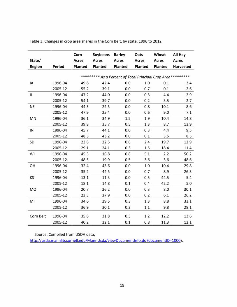
Tables 1 through 3 summarize changes in cropping patterns in the northern Corn Belt between 1996 and

2012, divided over the first part (1996-2004) and the second part (2005-2012) of the period. The tables

indicate that, relative to the first period, each state in our sample experienced an increase in corn acres

planted in the second period, both in absolute terms as well as measured as a proportion of total acres

planted. From the first to the second period, the regional average of the proportion of corn acres

planted out of total acres planted increased from 35.8 percent to 40.2 percent, while the proportion of

soybean acres out of total acres planted remained unchanged at about 32 percent. This indicates that

the increase in corn acres planted between the two periods took place at the expense of areas planted

to wheat, hay, and other crops. Furthermore, the increase in corn acre intensity suggests that producers

moved away from conventional crop rotation practices that included not only corn and soybeans but

other crops as well. These results are consistent with the findings of Wallander et al. (2011).

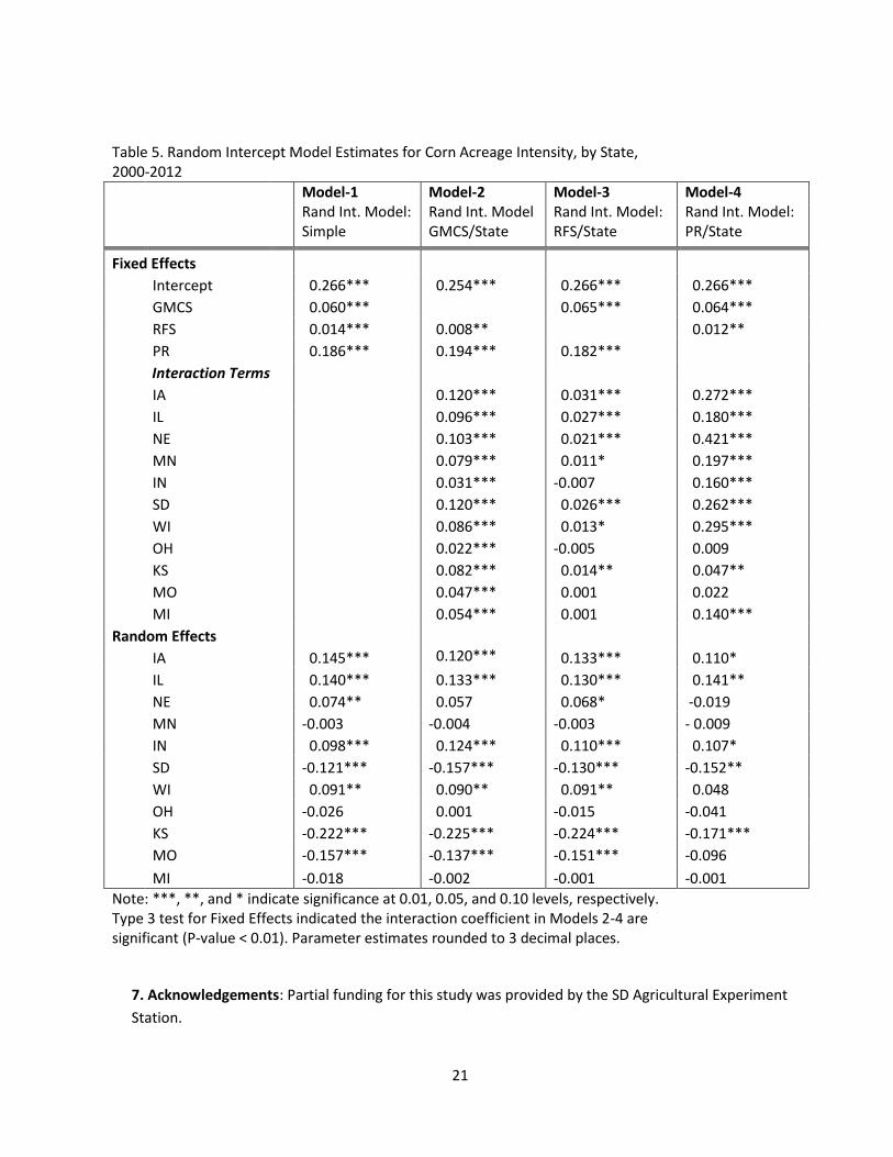
5.2 Regression Results

Four models were estimated: (a) Model-1, Simple Random Intercept Model, (b) Model-2, Random

Intercept Model with GMCS/State interaction terms, (c) Model-3, Random Intercept Model with

RFS/State interaction terms, and d) Model-4, Random Intercept Model with Price-Ratio/State interaction

terms. The fit statistics and regression results for the four estimated models used in our analysis are

provided in Tables 4 and 5. We provided estimated Intraclass Correlation Coefficients (ICC) for each

model (Table 4). The ICC estimates are greater than eighty percent for all four models. This statistical

evidence supports our conclusion that the effect of biotech advancements on producer planting

decisions are heterogeneous across states.

5.21 Model-1

Model-1 provides estimates for the fixed effects parameter estimates at the regional level. All

11

fixed effects parameter estimates are statistically significant at the one percent level. These findings

suggest that an increase in the corn-to-soybean price ratio, the adoption and diffusion of GM corn

technology, and the passage of the biofuels acts of 2005 and 2007 all positively affected corn acreage

intensity in the Corn Belt region. The fixed effects intercept has a value of 0.266, which can be

interpreted as an estimate of the regional average of the proportion of corn acres to total acres planted.

The random intercept coefficients reflect the deviation from the regional average. The coefficients for

KS, MO, and SD are statistically significant and negative, implying that these states’ intercepts are

smaller than the regional average intercept. The coefficients for MN, OH, and MI are not statistically

significant, implying that these states’ intercepts are at the regional average. The random intercept

coefficients of the remaining five states are statistically significant and positive, which implies that these

states’ intercepts are above the regional average. The simple mixed model confirms that GMCS adoption

rate, relative crop prices, and biofuel policy each contributed to an increase in corn acreage intensity in

the eleven states. Furthermore, the random intercept estimates confirm heterogeneity in cropping

decisions across states due to individual state attributes, including those related to agricultural

production and state-specific policies.

5.22 Model-2

In an effort to capture the state-specific effects of the adoption and diffusion of GM corn

technology on cropping pattern changes, we dropped the GMCS fixed effects variable and introduced

interaction terms (Model-2). The positive state-specific fixed effects slope coefficients for the

GMCS/State indicate that corn acreage intensity in all states was positively impacted by the

intensification of GM corn adoption. However, comparison of the state-specific GMCS interaction

coefficients in Model-2 with the GMCS coefficient (0.060) in Model-1 shows that in seven of the Corn

Belt states (IA, IL, KS, NE, MN, SD, and WI) the adoption and diffusion of transgenic corn varieties

disproportionately contributed to the increased corn acreage intensity in comparison to the region as a

12

whole. In the remaining four states (IN, OH, MO, and MI) the spread of GM corn varieties had a smaller

impact on corn acreage intensity relative to the regional average as estimated in Model-1. With respect

to the regional intercept and individual state random intercept estimates, the only noteworthy change

was that NE’s random intercept became insignificant. Regional fixed effects estimates for RFS and PR

remained positive and significant.

5.23 Model-3

Similarly, to assess the impact of the federal biofuel policy on cropping pattern changes by state,

we dropped the RFS as a regional explanatory variable and instead introduced state-specific RFS

interaction terms (Model-3). Comparing the state-specific fixed effects interaction coefficients in Model-

3 with the RFS coefficient (0.0136) in Model-1 helps identify those states where the RFS policies

intensified corn acreage plantings and where the effects are above the regional average.9 The results

indicate that the two federal biofuel laws had a disproportionately stronger impact on corn production

patterns in IA, IL, NE, and SD relative to the region overall. On the other hand, the impacts of federal

biofuel laws on cropping patterns in MN and WI were slightly below the regional average estimate

provided by model-1. This perhaps is due to state-level policies favoring biofuels production and usage

prior to the passage of federal regulations. The parameter estimates for the states in which the biofuel

laws had a particularly strong impact on changing cropping patterns (IA, IL, NE, and SD) were highly

significant, while those for the two states for which the biofuel laws had a slightly smaller impact than

for the northern Corn Belt region as a whole (MN and WI) were statistically significant at the five

percent level. The parameter estimate for KS was equal to that of the region overall, and was significant

at five percent. The parameter estimates for the remaining biofuel-state interaction terms (IN, MI, MO,

9 Given that RFS is a bivariate dummy variable, the parameter estimate for this variable represents a shift in

the intercept for the 2005-2012 period relative to the 2000 to 2004 period. In addition, an individual state’s intercept is a function of the regional fixed effects intercept plus the state’s individual random intercept estimate. Thus, the RFS interaction term provides an estimate of the shift in an individual state’s intercept due to biofuel legislation in the post 2004 period, relative to the pre-2004 period.

13

and OH) were not statistically significant. This implies that federal biofuel policy did not alter corn

acreage levels in these states relative to the 2000-2004. The unevenness of the effect of federal biofuel

policy on the proportion of corn acres planted suggests state-level idiosyncratic attributes played a role

in federal policy effectiveness. Regional fixed effects estimates for GMCS and PR remained positive and

significant.

5.24 Model-4

The final model investigates the effect of a change in relative crop price (PR) on a State’s corn

acreage intensity. In this model, we dropped the regional relative crop price variable and replaced it

with a State*PR interaction term. Similar to model 2, the interaction parameter estimates reflect

individual state fixed effects slope coefficients. The positive state-specific fixed effects slope coefficients

indicate that corn acreage intensity in nine of the states was positively impacted by an increase the

market price of corn relative to the price of soybeans. OH and MO had insignificant parameter

estimates, suggesting that corn acreage intensity was not affected by the PR ratio.

A comparison of the state-specific PR interaction coefficients in Model-4 with the PR coefficient

(0.1858) in Model-1 indicates that five of the states (IA, NE, MN, SD, and WI) had a significantly stronger

positive response to a change in relative price, as compared to the regional average with respect to corn

acre intensity. In four states (KS, MO, MI, and OH) the parameter estimates indicate a very weak corn

acreage response to a change in relative price compared to the regional average. The parameter

estimates for IL and IN indicate they had a similar acreage response to a change in relative prices in

comparison to the regional average. State heterogeneity also appears to be a viable explanation for the

variation in producer planting decision response to a change in relative crop price.

The Price-Ratio model’s regional fixed effects estimates for the intercept, the GMCS and RFS

parameters are very similar to simple model estimates. The random intercept assumption continued to

be statistically justified with a p-value less than 0.04 (the weakest of the four models). However, the

14

random intercept estimates for NE, WI, and MO became insignificant. Otherwise, the random intercept

estimates for Model-4 are consistent with Model-1.

5.3 Synopsis of Empirical Results

The parameter estimates of the random intercept component for the models 1-3 are highly

consistent, as are those of the fixed effects intercepts, which range from 0.254 to 0.266. This range

reflects the proportion of corn acres planted at the state level assuming that GM corn diffusion and

biofuel policies were unchanged. The random intercept is interpreted as the state-specific deviation

from the fixed effects intercept for the region as a whole. All states not having a statistically significant

random intercept reflect a proportion of corn acres planted equal to the regional average. These states

include MI, MN, and OH for all four models. Model-2 also includes NE and model-4 adds WI and MO.

States with statistically significant positive random intercept terms indicate that the proportions of corn

acres planted in these states were above the regional average prior the introduction of GM corn seed

and implementation of biofuel policies. The states with statistically significant and negative coefficients

represent those with less corn intensity than the regional average prior to the widespread diffusion of

GM corn and implementation of biofuel policy incentives.

One interesting insight gleaned from the parameter estimates for IN, MI, MO and OH is that

each of these states had GMCS/state interaction parameter estimates below the regional average

estimate provided in Model-1. These same states also were the only ones with insignificant RFS

interaction parameter estimates and these states were also less sensitive to changes in relative price as

compared to the regional state average. We conclude that these results suggest that the sensitivity of

corn acreage intensity to GMCS adoption and relative price changes are factors that affect biofuel policy

effectiveness in terms of changing corn acreage intensity. Thus we believe that the results indicate that

there is a positive relationship between increased GM corn diffusion and increasing corn acre intensity

due to the passage of biofuel policies. These results suggest that the sensitivity of corn acreage intensity

15

to the GM corn adoption contributed to the success of biofuel policy with respect to corn-starch based

ethanol production goals.

6. Discussion

Empirical evidence generated by a random intercept model with fixed effects indicates that the

intensification of corn acres planted was positively impacted by biotech advancements in energy and

agriculture. This suggests producers are moving away from diverse cropping patterns and the rotational

practices associated with a diverse crop planting strategy. As a result, total acres planted in small grains,

and hay has declined in the Corn Belt region. We conclude that corn acreage intensification can be

linked to past government policy decisions in the areas of energy and agriculture.

The empirical results presented demonstrate that state-level corn acreage intensification due to

the introduction of GM corn and biofuel technology was not homogenous across the eleven-state region

during the 13 year transition period covered in this study. The empirical results suggest that producer

corn acreage response to agriculture and energy policy decisions varies by geographical location. Thus,

future changes in ethanol energy policy, relative crop prices, and the ability of GM technology to provide

pest protection will also have a heterogeneous effect on producer cropping decisions. Future

agricultural policy decisions need to recognize that producer reaction to changes in the above factors

will depend on geographical location.

The evidence also suggests that the significant increase in corn acreage intensity over the period

of analysis is linked to biofuel policies and GM corn adoption. Furthermore, the proportion of soybean

acres has remained stable in the pre- and post-RFS periods. This indicates a decline in the acres

allocated to alternative crops used in conventional rotation practices in the region (Table 1). Empirical

evidence also indicates that five of the eleven states (IA, IL, KS, MO, and SD) experienced a double-digit

percentage increase in corn acres planted between the two periods. This suggests that the effects of

16

using GM corn technology on the production side and biofuel policies on the demand side vary by state.

Empirical evidence suggests that IN, MI, MO, and OH experienced a below-average boost from the use

of GM corn on corn acres planted. These four states were also the one where biofuel policy had no

effect on corn intensity. The identification of the heterogonous factors across states may provide

additional insights on how cropping patterns will change in the future in response to policy changes.

Cropping pattern changes in general and the growing dominance of corn in U.S. crop production

systems in the eleven states have shed light on host of expected and unexpected consequences. For

example, the relatively high corn prices experienced over the past several years contributed to a decline

in the production of other crops, price increases of other crops globally, and an increase in the cost of

raising livestock. Corn production intensification facilitated in part by the reliance on GM varieties also

resulted in increased corn pest resistance (e.g., Gassmann et al. 2011) and increased planted acre

coverage with insecticide (Fausti et al. 2012). Both the extent of the pest resistance and the subsequent

increase in insecticide-acreage-coverage were unanticipated at the onset of the widespread use of crop

biotechnology.

While based on data collected in the eleven-state region sometimes referred to as the U.S. Corn

Belt, this study is also of interest to other regions of the United States. Corn production has expanded

not only in response to the widespread adoption of GM corn varieties and biofuel policies, but also as a

consequence of other forces such as climate change and plant breeding technology improvements.

Thus, the issues addressed in our study represent a challenge for and are of critical importance to

agriculture in the future throughout the United States.

17

Table 1. Changes in principal crops area in the Corn Belt, 1996 to 2012

Avg. (1996-2004) Avg. (2005-2012) Change in Area

Crops 1,000 acres % 1,000 acres % 1,000 acres %

Corn, Planted Acres 64283 35.8 71044 40.2 6760 11

Soybean, Planted Acres 57103 31.8 56651 32.1 -452 -1

Barley1, Planted Acres 524 0.3 226 0.1 -297 -57

Oats1, Planted Acres 2077 1.2 1378 0.8 -699 -34

Wheat, Planted Acres 22331 12.4 20053 11.3 -2278 -10

Hay, Harvested Acres 24375 13.6 21454 12.1 -2921 -12

Others 8886 4.9 5945 3.4 -3727 -41.9

Total Planted Area 179580 100.0 176751 100.0 -2829 -2

1 Oats: Avena sativa; Barley: Hordeum vulgare. Source: Compiled from USDA data,

http://usda.mannlib.cornell.edu/MannUsda/viewDocumentInfo.do?documentID=1000).

18

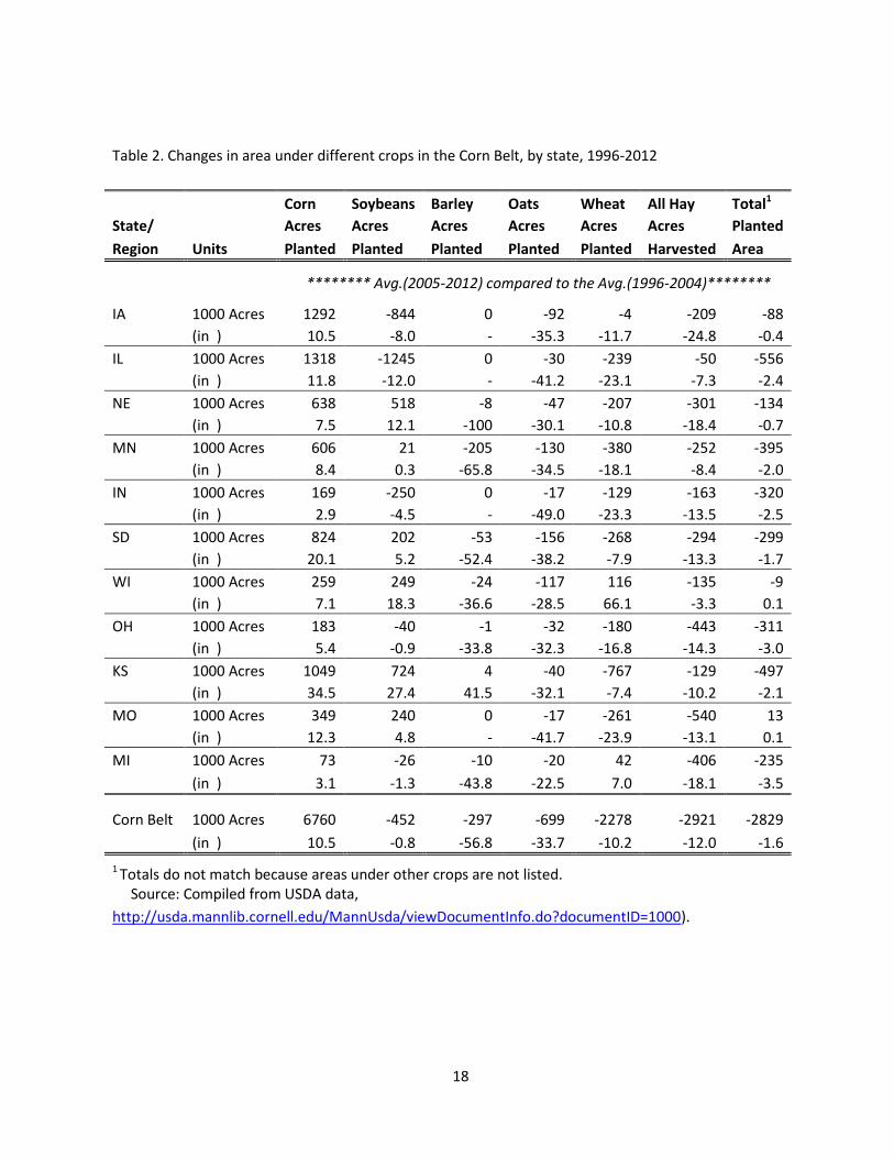
Table 2. Changes in area under different crops in the Corn Belt, by state, 1996-2012

Corn Soybeans Barley Oats Wheat All Hay Total1

State/

Acres Acres Acres Acres Acres Acres Planted

Region Units Planted Planted Planted Planted Planted Harvested Area

******** Avg.(2005-2012) compared to the Avg.(1996-2004)********

IA 1000 Acres 1292 -844 0 -92 -4 -209 -88

(in ) 10.5 -8.0 - -35.3 -11.7 -24.8 -0.4

IL 1000 Acres 1318 -1245 0 -30 -239 -50 -556

(in ) 11.8 -12.0 - -41.2 -23.1 -7.3 -2.4

NE 1000 Acres 638 518 -8 -47 -207 -301 -134

(in ) 7.5 12.1 -100 -30.1 -10.8 -18.4 -0.7

MN 1000 Acres 606 21 -205 -130 -380 -252 -395

(in ) 8.4 0.3 -65.8 -34.5 -18.1 -8.4 -2.0

IN 1000 Acres 169 -250 0 -17 -129 -163 -320

(in ) 2.9 -4.5 - -49.0 -23.3 -13.5 -2.5

SD 1000 Acres 824 202 -53 -156 -268 -294 -299

(in ) 20.1 5.2 -52.4 -38.2 -7.9 -13.3 -1.7

WI 1000 Acres 259 249 -24 -117 116 -135 -9

(in ) 7.1 18.3 -36.6 -28.5 66.1 -3.3 0.1

OH 1000 Acres 183 -40 -1 -32 -180 -443 -311

(in ) 5.4 -0.9 -33.8 -32.3 -16.8 -14.3 -3.0

KS 1000 Acres 1049 724 4 -40 -767 -129 -497

(in ) 34.5 27.4 41.5 -32.1 -7.4 -10.2 -2.1

MO 1000 Acres 349 240 0 -17 -261 -540 13

(in ) 12.3 4.8 - -41.7 -23.9 -13.1 0.1

MI 1000 Acres 73 -26 -10 -20 42 -406 -235

(in ) 3.1 -1.3 -43.8 -22.5 7.0 -18.1 -3.5

Corn Belt 1000 Acres 6760 -452 -297 -699 -2278 -2921 -2829

(in ) 10.5 -0.8 -56.8 -33.7 -10.2 -12.0 -1.6

1 Totals do not match because areas under other crops are not listed. Source: Compiled from USDA data,

http://usda.mannlib.cornell.edu/MannUsda/viewDocumentInfo.do?documentID=1000).

19

Table 3. Changes in crop area shares in the Corn Belt, by state, 1996 to 2012

Corn Soybeans Barley Oats Wheat All Hay

State/

Acres Acres Acres Acres Acres Acres

Region Period Planted Planted Planted Planted Planted Harvested

********* As a Percent of Total Principal Crop Area*********

IA 1996-04 49.8 42.4 0.0 1.0 0.1 3.4

2005-12 55.2 39.1 0.0 0.7 0.1 2.6

IL 1996-04 47.2 44.0 0.0 0.3 4.4 2.9

2005-12 54.1 39.7 0.0 0.2 3.5 2.7

NE 1996-04 44.3 22.5 0.0 0.8 10.1 8.6

2005-12 47.9 25.4 0.0 0.6 9.0 7.1

MN 1996-04 36.1 34.9 1.5 1.9 10.4 14.8

2005-12 39.8 35.7 0.5 1.3 8.7 13.9

IN 1996-04 45.7 44.1 0.0 0.3 4.4 9.5

2005-12 48.3 43.2 0.0 0.1 3.5 8.5

SD 1996-04 23.8 22.5 0.6 2.4 19.7 12.9

2005-12 29.1 24.1 0.3 1.5 18.4 11.4

WI 1996-04 45.3 16.8 0.8 5.1 2.2 50.2

2005-12 48.5 19.9 0.5 3.6 3.6 48.6

OH 1996-04 32.4 43.6 0.0 1.0 10.4 29.8

2005-12 35.2 44.5 0.0 0.7 8.9 26.3

KS 1996-04 13.1 11.3 0.0 0.5 44.5 5.4

2005-12 18.1 14.8 0.1 0.4 42.2 5.0

MO 1996-04 20.7 36.2 0.0 0.3 8.0 30.1

2005-12 23.3 37.9 0.0 0.2 6.1 26.2

MI 1996-04 34.6 29.5 0.3 1.3 8.8 33.1

2005-12 36.9 30.1 0.2 1.1 9.8 28.1

Corn Belt 1996-04 35.8 31.8 0.3 1.2 12.2 13.6

2005-12 40.2 32.1 0.1 0.8 11.3 12.1

Source: Compiled from USDA data,

http://usda.mannlib.cornell.edu/MannUsda/viewDocumentInfo.do?documentID=1000).

20

Table 4. Variance Components Statistics and Global Fit Statistics

Model-1 Model-2 Model-3 Model-4

Rand Int. Model: Simple

Rand Int. Model: GMCS/State

Rand Int. Model: RFS/State

Rand Int. Model: PR/State

Covariance Parameter

Covariance Par Est. & Z statistic

Covariance Par Est. & Z statistic

Covariance Par Est. & Z statistic

Covariance Par Est. & Z statistic

Random Int. 0.01541: Z=2.23 0.01544: Z=2.20 0.01505: Z=2.23 0.01386: Z=1.75

Residual 0.000329: Z=8.03 0.000329: Z=7.71 0.000311: Z=7.71 0.000337: Z=7.71

Intraclass Corr coef. ICC = 82.4% ICC = 84% ICC = 83% ICC= 80%

Fit Statistics

-2 Log Likelihood -648.6 -619.7 -594.9 -638.1

AIC -644.6 -615.7 -590.9 -634.1

BIC -643.8 -614.9 -590.1 -633.3

21

Table 5. Random Intercept Model Estimates for Corn Acreage Intensity, by State, 2000-2012

Model-1 Rand Int. Model: Simple

Model-2 Rand Int. Model GMCS/State

Model-3 Rand Int. Model: RFS/State

Model-4 Rand Int. Model: PR/State

Fixed Effects

Intercept 0.266*** 0.254*** 0.266*** 0.266***

GMCS 0.060*** 0.065*** 0.064***

RFS 0.014*** 0.008** 0.012**

PR 0.186*** 0.194*** 0.182***

Interaction Terms

IA

0.120*** 0.031*** 0.272***

IL

0.096*** 0.027*** 0.180***

NE

0.103*** 0.021*** 0.421***

MN

0.079*** 0.011* 0.197***

IN

0.031*** -0.007 0.160***

SD

0.120*** 0.026*** 0.262***

WI

0.086*** 0.013* 0.295***

OH

0.022*** -0.005 0.009

KS

0.082*** 0.014** 0.047**

MO

0.047*** 0.001 0.022

MI

0.054*** 0.001 0.140***

Random Effects

IA

0.145*** 0.120*** 0.133*** 0.110*

IL

0.140*** 0.133*** 0.130*** 0.141**

NE

0.074** 0.057 0.068* -0.019

MN

-0.003 -0.004 -0.003 - 0.009

IN

0.098*** 0.124*** 0.110*** 0.107*

SD

-0.121*** -0.157*** -0.130*** -0.152**

WI

0.091** 0.090** 0.091** 0.048

OH

-0.026 0.001 -0.015 -0.041

KS

-0.222*** -0.225*** -0.224*** -0.171***

MO

-0.157*** -0.137*** -0.151*** -0.096

MI -0.018 -0.002 -0.001 -0.001

Note: ***, **, and * indicate significance at 0.01, 0.05, and 0.10 levels, respectively. Type 3 test for Fixed Effects indicated the interaction coefficient in Models 2-4 are significant (P-value < 0.01). Parameter estimates rounded to 3 decimal places.

7. Acknowledgements: Partial funding for this study was provided by the SD Agricultural Experiment

Station.

22

8. References Benbrook, C., & InfoNet, B. (2004). Genetically engineered crops and pesticide use in the United States: the first nine years. Union of Concerned Scientists. Benbrook, C. (2009). Impacts of genetically engineered crops on pesticide use: The first thirteen years. The Organic Center, November. Cai, X., & Stiegert, K. W. (2014). Market Analysis of Ethanol Capacity. International Food and Agribusiness Management Review, 17(1), 83. Cap, E., & Malach, V. (2012, June). The Changing Patterns In Land Allocation To Soybeans And Maize In Argentina And The Americas And The Role Of Gm Varieties. A Comparative Analysis. In 2012 Conference, August 18-24, 2012, Foz do Iguacu, Brazil (No. 126376). International Association of Agricultural Economists. Cattaneo, M. G., Yafuso, C., Schmidt, C., Huang, C. Y., Rahman, M., Olson, C., ... & Carriere, Y. (2006). Farm-scale evaluation of the impacts of transgenic cotton on biodiversity, pesticide use, and yield. Proceedings of the National Academy of Sciences, 103(20), 7571-7576. Claassen, R., Carriazo, F., and Ueda, K. (2010). “Grassland Conversion for Crop Production in the United States: Defining Indicators for Policy Analysis.” OECD Agri-environmental Indicators: Lessons Learned and Future Directions. http://www.oecd.org/tad/sustainable-agriculture/44807867.pdf Diggle, P., Liang, K. and Zeger, S. (1994), Analysis of Longitudinal Data, Oxford: Clarendon Press. Economic Research Service (2014). “Genetically Engineered Varieties of Corn, upland cotton, and soybeans, by State and for the Unites States, 2000-13.” Data Set Accessed January 15, 2014. http://www.ers.usda.gov/datafiles/Adoption_of_Genetically_Engineered_Crops_in_the_US/alltables.xls Environmental Protection Agency (2014). Web Page: http://www.epa.gov/mtbe/gas.htm Accessed January 15, 2014. Fausti, S. W., McDonald, T. M., Lundgren, J. G., Li, J., Keating, A. R., & Catangui, M. (2012). Insecticide use and crop selection in regions with high GM adoption rates. Renewable Agriculture and Food Systems, 27(04), 295-304. Fernandez-Cornejo, J., & McBride, W. D. (2002). Adoption of bioengineered crops. ERS Agricultural Economic Report No. AER810. Fernandez-Cornejo, J., Wechsler, S., Livingston, M., & Mitchell, L. (2014). Genetically Engineered Crops in the United States (No. 164263). United States Department of Agriculture, Economic Research Service. Food and Agricultural Policy Research Institute (2014). Biofuel Conversion Factors 2005 and 2012. Web Page: http://www.fapri.missouri.edu/outreach/publications/2006/biofuelconversions.pdf. Accessed January 15, 2014.

23

Gassmann, A. J., Petzold-Maxwell, J. L., Keweshan, R. S., & Dunbar, M. W. (2011). Field-evolved resistance to Bt maize by western corn rootworm. PLoS One, 6(7), e22629. Hutchison, W. D., Burkness, E. C., Mitchell, P. D., Moon, R. D., Leslie, T. W., Fleischer, S. J., ... & Raun, E. S. (2010). Areawide suppression of European corn borer with Bt maize reaps savings to non-Bt maize growers. Science, 330(6001), 222-225. Johnston, C. A. (2014). Agricultural expansion: land use shell game in the US Northern Plains. Landscape Ecology, 29(1), 81-95. Landis, D. A., Gardiner, M. M., van der Werf, W., & Swinton, S. M. (2008). Increasing corn for biofuel production reduces biocontrol services in agricultural landscapes. Proceedings of the National Academy of Sciences, 105(51), 20552-20557. Mercier, S. (2011). “Review of U.S. Food and Ag. Policy.” http://foodandagpolicy.org/policy/publications. National Agricultural Statistics Service. (2014). USDA Economics, Statistics and Market Information System, Albert R. Mann Library, Cornell University. Web Site: http://usda.mannlib.cornell.edu/MannUsda/viewDocumentInfo.do?documentID=1000 Accessed January 15, 2014. Renewable Fuels Association (2014). Web Page: (http://www.ethanolrfa.org/) Accessed January 15, 2014. SAS Institute. (2011). SAS/STAT® User’s Guide: Chapter 6, Version 9.3. Cary, NC: SAS Institute Inc: http://support.sas.com/documentation/cdl/en/statug/63962/HTML/default/viewer.htm#statug_mixed_sect003.htm Accessed October 2013. SAS Institute. (1999). SAS/STAT® User’s Guide: Chapter 41, Version 8. Cary, NC: SAS Institute Inc. Scandizzo, P. L., & Savastano, S. (2010). The adoption and diffusion of GM crops in United States: A real option approach. Ag Bio Forum 13(2), 142-157. Schnepf, R., & Yacobucci, B. D. (2013). Renewable Fuel Standard (RFS): overview and issues. Congressional Research Service: Washington, DC. http://www.fas.org/sgp/crs/misc/R40155.pdf Accessed January 15, 2014. Van der Sluis, E., Diersen, M. A., & Dobbs, T. L. (2002). Agricultural biotechnology: Farm-level, market, and policy considerations. Journal of Agribusiness, 20(1), 51-66. Wallander, S., Claassen, R., & Nickerson, C. J. (2011). The ethanol decade: an expansion of US corn production, 2000-09 (No. 117982). United States Department of Agriculture, Economic Research Service.

24