The effect of high temperature induced variation of specific heat on the hypersonic turbulent boundary layer and its computation

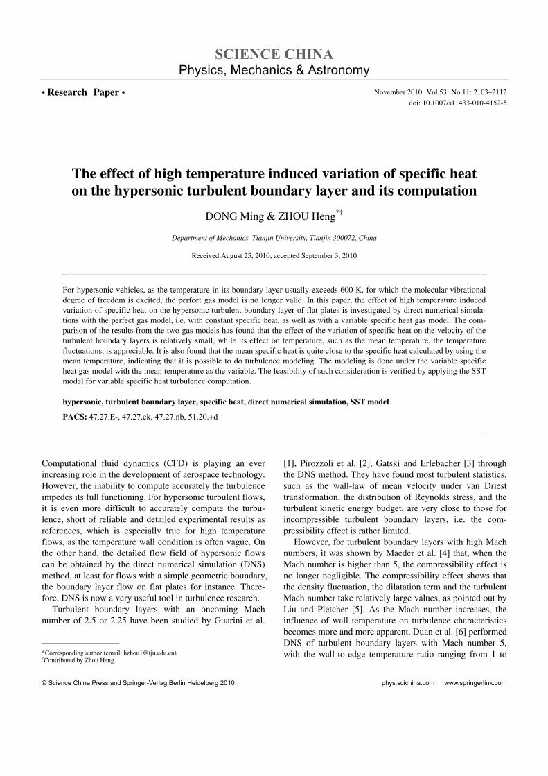
SCIENCE CHINA Physics, Mechanics & Astronomy

© Science China Press and Springer-Verlag Berlin Heidelberg 2010 phys.scichina.com www.springerlink.com

*Corresponding author (email: [email protected]) †Contributed by Zhou Heng

• Research Paper • November 2010 Vol.53 No.11: 2103–2112

doi: 10.1007/s11433-010-4152-5

The effect of high temperature induced variation of specific heat on the hypersonic turbulent boundary layer and its computation

DONG Ming & ZHOU Heng*†

Department of Mechanics, Tianjin University, Tianjin 300072, China

Received August 25, 2010; accepted September 3, 2010

For hypersonic vehicles, as the temperature in its boundary layer usually exceeds 600 K, for which the molecular vibrational degree of freedom is excited, the perfect gas model is no longer valid. In this paper, the effect of high temperature induced variation of specific heat on the hypersonic turbulent boundary layer of flat plates is investigated by direct numerical simula-tions with the perfect gas model, i.e. with constant specific heat, as well as with a variable specific heat gas model. The com-parison of the results from the two gas models has found that the effect of the variation of specific heat on the velocity of the turbulent boundary layers is relatively small, while its effect on temperature, such as the mean temperature, the temperature fluctuations, is appreciable. It is also found that the mean specific heat is quite close to the specific heat calculated by using the mean temperature, indicating that it is possible to do turbulence modeling. The modeling is done under the variable specific heat gas model with the mean temperature as the variable. The feasibility of such consideration is verified by applying the SST model for variable specific heat turbulence computation.

hypersonic, turbulent boundary layer, specific heat, direct numerical simulation, SST model

PACS: 47.27.E-, 47.27.ek, 47.27.nb, 51.20.+d

Computational fluid dynamics (CFD) is playing an ever increasing role in the development of aerospace technology. However, the inability to compute accurately the turbulence impedes its full functioning. For hypersonic turbulent flows, it is even more difficult to accurately compute the turbu-lence, short of reliable and detailed experimental results as references, which is especially true for high temperature flows, as the temperature wall condition is often vague. On the other hand, the detailed flow field of hypersonic flows can be obtained by the direct numerical simulation (DNS) method, at least for flows with a simple geometric boundary, the boundary layer flow on flat plates for instance. There-fore, DNS is now a very useful tool in turbulence research.

Turbulent boundary layers with an oncoming Mach number of 2.5 or 2.25 have been studied by Guarini et al.

[1], Pirozzoli et al. [2], Gatski and Erlebacher [3] through the DNS method. They have found most turbulent statistics, such as the wall-law of mean velocity under van Driest transformation, the distribution of Reynolds stress, and the turbulent kinetic energy budget, are very close to those for incompressible turbulent boundary layers, i.e. the com-pressibility effect is rather limited.

However, for turbulent boundary layers with high Mach numbers, it was shown by Maeder et al. [4] that, when the Mach number is higher than 5, the compressibility effect is no longer negligible. The compressibility effect shows that the density fluctuation, the dilatation term and the turbulent Mach number take relatively large values, as pointed out by Liu and Pletcher [5]. As the Mach number increases, the influence of wall temperature on turbulence characteristics becomes more and more apparent. Duan et al. [6] performed DNS of turbulent boundary layers with Mach number 5, with the wall-to-edge temperature ratio ranging from 1 to

2104 DONG Ming, et al. Sci China Phys Mech Astron November (2010) Vol. 53 No. 11

5.4. They found that as the wall temperature decreases, the compressibility effect increases, and the near wall turbulent structures become much less chaotic.

All the mentioned work of DNS used the perfect gas model, so the specific heat was taken as a constant. How-ever, when the temperature in boundary layers exceeds 600 K, the vibrational degrees of freedom of nitrogen and oxy-gen molecules are excited, so the specific heat is no longer constant, neither the perfect gas model is appropriate. If the temperature is higher than 2500 K, the dissociation and chemical reaction of the molecules should also be taken into account.

For a high Mach number in laboratories, the temperatures of the oncoming flow are often reduced to a very low level, usually several tens of K. In those cases, even if the Mach number reaches 6, the highest temperature in the boundary layer is still lower than 600 K, implying the variation of specific heat unnecessary. Thus in performing DNS of tur-bulent boundary layers with oncoming Mach number 6, Dong et al. [7–9] still used the perfect gas model, because the oncoming temperatures were only 79 K, in accordance with corresponding experiments. However, for real flying vehicles, the environmental temperature is usually of the order 200 K, so the highest temperature in the boundary layer can exceed 1500 K, if the flying Mach number is 6, which means that the perfect gas model is no longer valid. The consequence is, the experiments done in the laboratory may not produce results directly corresponding to the real flight condition. In such cases, DNS becomes a useful tool for the study of turbulent boundary layers by using gas models with real gas effects being taken into consideration.

In fact, Malik and Anderson [10] did a stability analysis of hypersonic boundary layer with the vibrational degree of freedom and dissociation of molecules being taken into consideration, and they found that the first mode waves be-came more stable, whereas the second mode waves became more unstable. Jia and Cao [11] also studied the influence of variable specific heat on the stability of hypersonic boundary layers. Hornung [12] studied the problem of hy-personic real gas effect on transition. Apparently, the varia-tion of specific heat also influences the turbulence charac-teristics in turbulent boundary layers. To correctly predict the heat flux of flying vehicles must include the variable specific heat due to a high temperature.

In this paper, three cases of hypersonic turbulent bound-ary layers, in which the highest temperatures are still below 2500 K, are computed with both the perfect gas model and the variable specific heat gas model, to study the influence of variable specific heat on the turbulence characteristics.

Although we can use DNS to study turbulent flows with simple geometric boundaries, it is highly unrealistic to use DNS for engineering designs, for which turbulence model-ing is still the only practical method. However, the existing turbulence models are always based on the perfect gas model. If the gas is imperfect, additional variables would

appear, implying that we need additional governing equa-tions, unless the average specific heat ratio can be obtained by simply referring to average temperature. This paper will prove that this is indeed approximately true, and verify the feasibility of turbulence modeling under the variable spe-cific heat gas model by applying the SST turbulence model [13] to the hypersonic turbulent boundary layer with vari-able specific heat.

1 Method of direct numerical simulation

1.1 Governing equations

The nondimensional continuity, momentum and energy equations are

( ) 0

( ) 0

[( ) ] 0

jj

ii j ij ij

j

ss j i ij j

j

ut x

uu u p

t x

ee p u u q

t x

ρ ρ

ρρ δ σ

ρρ σ

⎧∂ ∂+ =⎪

∂ ∂⎪⎪∂ ∂⎪ + + − =⎨

∂ ∂⎪⎪∂ ∂⎪ + + − + =

∂ ∂⎪⎩

(1)

where, , , [ , , ]jp u u v wρ = are the density, pressure and

velocity with stream-wise, normal-wise and span-wise

components u, v, w, respectively; 2

2 ,3ij ij ij kkS Sσ μ μδ= −

the viscous stress tensor, ( / / ) / 2,ij i j j iS u x u x= ∂ ∂ + ∂ ∂ the

strain tensor; μ, the viscosity coefficient, ,ijδ the unit ten-

sor; / ,j jq T xκ= − ∂ ∂ the heat flux, and κ is the heat con-

ductivity coefficient; es, the unit total energy, M, the Mach number, and γ, the specific heat ratio.

In addition, the state equation reads

2/ .P T Mρ γ= (2)

For the perfect gas model, the specific heat is taken as constant, the specific heat ratio 1.4,γ = and the unit total

energy 2/ [ ( 1) ] / 2.s i ie T M u uγ γ= − +

For the variable specific heat gas model with a tempera-ture higher than 600 K, but below 2500 K, the specific heat can be expressed as a function of temperature [14]. For the specific heat with a constant volume, it is

2 /

/ 2

5 e( ) ,

2 (e 1)

ve

ve

T Tve

v T T

Tc T R R

T

⎛ ⎞= + ⎜ ⎟ −⎝ ⎠ (3)

while for the specific heat with a constant pressure, it is

2 /

/ 2

7 e( ) ,

2 (e 1)

ve

ve

T Tve

p T T

Tc T R R

T

⎛ ⎞= + ⎜ ⎟ −⎝ ⎠ (4)

DONG Ming, et al. Sci China Phys Mech Astron November (2010) Vol. 53 No. 11 2105

where veT is a temperature representing the vibrational

characteristics of molecules, selected to be 3030 K [11], and R is the gas constant.

Then the specific heat ratio can be expressed as:

2 /

/ 2

2 /

/ 2

7 e( ) 2 (e 1)

( ) .( ) 5 e

2 (e 1)

ve

ve

ve

ve

T Tve

T Tp

T Tv ve

T T

Tc T T

Tc T T

T

γ

⎛ ⎞+ ⎜ ⎟ −⎝ ⎠= =⎛ ⎞+ ⎜ ⎟ −⎝ ⎠

(5)

The unit total energy can be expressed as:

2/

5( ) / 2.

2 e 1ve

ves i iT T

Te T M u uγ⎡ ⎤= + +⎢ ⎥−⎣ ⎦

(6)

1.2 Difference scheme, computational mesh and boundary conditions

The non-linear terms in eq. (1) are computed by the 7th or-der upwind difference scheme, the viscous terms are com-puted by the 6th order central difference scheme, and the time derivative terms are computed by the 2nd order Runge-Kutta method.

Uniform meshes are adopted in the stream-wise direction, the mesh size is *

00.2 ,δ where *0δ is the displacement

thickness of the boundary layer at the inlet of the computa-tional domain, the number of grids is 1101, and the stream-wise extent of the computational domain is 220 *

0 ;δ

non-uniform meshes are adopted in the normal-wise direc-tion, the number of grids is 61, the normal-wise extent of computational domain is 40 *

0 ,δ and the mesh size at the

wall is 0.00513 *0 ;δ uniform meshes are adopted in the

span-wise direction, the mesh size is 0.2045 *0 ,δ and the

number of grids is 256. Non-slip and adiabatic or isothermal conditions are em-

ployed at the wall, and the boundary conditions at the upper boundary of the computational domain are set by the on-coming flow; periodic boundary conditions are employed in the span-wise direction. A buffer zone is added downstream to the effective computational domain, and the stream-wise grid number is 100.

For DNS of the turbulent boundary layer, we need an appropriate inflow condition. The most effective way to specify the inflow condition is to use a known turbulent flow field, obtained by the temporal mode DNS of a turbu-lent flow with the same boundary condition, the same Mach number and the same Reynolds number [15]. But we can even specify the inflow condition by using the flow field obtained by the temporal mode DNS for turbulent flow with a different Mach number, a different Reynolds number, and a different temperature condition, (see [8,9]). In this paper, the latter method is employed, and there will be a transient section downstream of the inlet for the turbulent flow to

become fully developed, and the length of the transient sec-tion is about 100 *

0δ in the stream-wise direction, which

will be discarded before analyzing the results. The results shown in the subsequent Figures, with the stream-wise length of about 120 *

0 ,δ do not include this transient zone.

2 Cases computed

The parameters for the three cases studied are shown in Ta-ble 1, in which x0 represents the distance between the lead-ing edge of the plate and the upstream bound of the final useful section of the computational domain. Case I and Case II have the same Mach number, but with different wall temperature conditions, while Case I and Case III share the same wall temperature condition, but with a different Mach number. Under the perfect gas model, when the oncoming Mach number is 7.4, the adiabatic wall temperature will be about 10.75Te, or about 2435 K, which almost reaches the upper limit for the validity of eq. (5). Therefore, in this paper, cases with a Mach number higher than 7.4 are not studied.

The oncoming flow corresponds to the condition of air at a height of 30000 meters above the sea level, for which the temperature is 226.5 K, the acoustic speed is 301.7 m/s, the density is 0.01841 kg/m3, and the kinematic viscosity coef-ficient is 1.475×10−5 Pa s. The Reynolds number based on the displacement thickness *

0δ at the entrance of the com-

putational domain is 10000. Each case is computed by two different gas models: model (i), the perfect gas model with the specific heat ratio 1.4γ = ; model (ii), the variable spe-

cific heat gas model with the specific heat ratio being de-termined by eq. (5).

3 Verification of DNS results

When the statistics of compressible turbulent flows are studied, the variation of density should be considered. So both the Favre average and Reynolds average are intro-duced:

,u u u u u′ ′′= + = + (7)

Table 1 Parameters for the three cases studied

Case number

Gas model

Mach number

Wall temperature condition

*0δ (mm) x0

(m) Case I-i i

Case I-ii ii 6 adiabatic 4.4 0.70

Case II-i i

Case II-ii ii 6 Isothermal Tw=3 4.4 0.70

Case III-i i

Case III-ii ii 7.4 adiabatic 3.6 0.48


where u is the Reynolds averaged value and u the Favre averaged value of the quantity u, while u′ and u′′ are the fluctuations under Reynolds average and Favre average

respectively. The relationship /u uρ ρ= holds.

3.1 Comparison of results with different mesh sizes

In order to ensure a sufficiently fine mesh size, the mesh size is refined in either the stream-wise or the span-wise direction for Case I-i, and then results are compared, as shown in Figure 1. The solid line represents the results with the mesh size stated in sec. 1.2, the dashed line represents the results with the mesh number doubled in the x direction, and the dot dashed line represents the results with the mesh number doubled in the z direction. The abscissa in Figure 1(a) represents the stream-wise coordinate x, while the or-dinate represents the wall friction coefficient (Cf curve) whose definition is as follows:

w2

,/ 2fC

u

τρ∞ ∞

= (8)

where, /u yτ μ= ∂ ∂ represents the viscous stress, the

subscript w implies its value at the wall, and the subscript ∞ implies the value of the oncoming flow. The abscissa in Figure 1(b) represents either the stream-wise mean velocity or the mean temperature, while the ordinate represents the normal-wise coordinate. Clearly the results remain almost unchanged as the mesh size is refined, implying the mesh size adopted in this paper is fine enough.

3.2 Comparison of the results with those in other re-ports

The results in Case I-i are compared with those in other reports.

The comparison of wall friction coefficient is shown in Figure 2, where the abscissa represents the Reynolds num-ber based on the momentum thickness Reθ, the solid line is

the result computed in this paper, and the filled square symbol is the results of DNS for the Mach number 6 turbu-lent boundary layer on a flat plate computed by Maeder et al. [4]. It can be seen the trend of the two results are consistent.

The comparison of the near-wall-law of the mean stream-wise velocity is shown in Figure 3, where the solid line is the results computed by Li et al. [16] for a Mach number 6 turbulent boundary layer on a flat with Reθ =1.095 ×105, the dot dashed line is the results computed in this pa-per, and the dashed lines are the linear-law and log-law curves respectively. The abscissa is the normal-wise coor-dinate expressed in a wall unit; whereas the ordinate is the mean stream-wise velocity under the van Driest transforma-tion, also expressed in a wall unit. The definition is as fol-lows:

1/2

0( / ) d .

u

c wu uρ ρ+

+ += ∫ (9)

It can be seen that, in the region 200,y+ < which contains

the linear-law region and a part of log-law region, the re-sults computed in this paper agree well with that computed by Li, while in the outer region, the two curves differ from each other, because the Reynolds number differs for the two cases, which in turn implies the difference of the thickness of boundary layer for the two cases.

The comparison of turbulence intensity is shown in Fig-ure 4. The ordinate is the turbulence intensity, i.e. the ratio of the root-mean-square value of velocity fluctuations with respect to the mean stream-wise velocity. In the figure, the unfilled symbols represent the experimental results of in-compressible turbulent flows, the lines without a symbol are the results of Li et al. [16], and the solid lines with filled symbols are our results. As can be seen that, our rms /w w′

agrees well with the results of Li et al., but for rms /u u′ and

rms / ,v v′ they are not completely identical, with yet similar

general trends. The incomplete agreement may be due to the major difference of Reynolds numbers between ours and those of Li et al.

Figure 1 Comparison of the results with the mesh refined. (a) The wall friction coefficient; (b) the mean profile.


Figure 2 Comparison of the wall friction coefficient.

Figure 3 Comparison of the near-wall-law.

Figure 4 The turbulence intensity.

The governing equation of turbulent kinetic energy

/ 2i ik u u′′ ′′= in compressible flow can be written as:

( ) ,t dk C P T D Mt

ρ ε∂= − + + + Π + Π + + −

∂ (10)

where, ( ) /j jC u k xρ= −∂ ∂ is the contribution to the turbu-

lent kinetic energy from the nonlinear convection term,

/ ,i j i jP u u u xρ ′′ ′′= − ∂ ∂ the production from the mean veloc-

ity gradient, ( / 2) / ,i i j jT u u u xρ ′′ ′′ ′′= −∂ ∂ the turbulent trans-

port term, ( ) / ,t j jp u x′ ′′Π = −∂ ∂ the pressure diffusion term,

/ ,d i ip u x′ ′′Π = ∂ ∂ the pressure dilatation term, D =

( ) / ,i ij iu xσ′′ ′∂ ∂ the viscous diffusion term, ( /i ij jM u xσ′′= ∂ ∂

/ ),ip x−∂ ∂ the mass flux contribution associated to density

fluctuations, and / ,ij i ju xε σ ′ ′′= ∂ ∂ the viscous dissipation.

The comparisons of P, T, D and −ε are shown in Figure 5, with other terms neglected out of their smallness. In the figure, the dashed lines represent the results of a Mach number 2.25 flat plate turbulent boundary layer, computed by Pirozzoli et al. [2], the solid lines represent the results computed by Li et al. [16], and curves with symbols are our results. It can be seen that, the T, D and −ε terms are all close to Li’s results, with a poor agreement of P term in the region y+>10, because this term depends explicitly on the mean velocity gradient. In Li et al.’s case, the Reynolds number is much larger than ours, implying that their bound-ary layer thickness is much larger than ours. The distribu-tions of the mean velocity gradient in their case must be appreciably different from our case under the y+ coordinate.

4 Results of DNS

4.1 Wall friction coefficient and boundary layer thick-ness

The stream-wise distribution of wall friction coefficients are shown in Figure 6, where the solid lines are the results of the perfect gas model, while the dashed lines are the results of the variable γ gas model. As can be seen, the difference of results from the two gas models is almost negligible. It is because the constant or variable γ only affects velocity in-directly through viscosity, which implicitly depends, while not strongly, on temperature.

The stream-wise distributions of the displacement thick-

Figure 5 The turbulent kinetic energy budget.


Figure 6 Cf curves.

nesses of the boundary layer are shown in Figure 7, where the definition of the lines is the same as for Figure 6. The displacement thickness of a boundary layer is defined as:

*

0e e

1 d ,u

yu

δ ρδρ

⎛ ⎞= −⎜ ⎟

⎝ ⎠∫ (11)

where δ is the nominal boundary layer thickness, and the subscript ‘e’ refers to the value at the edge of the boundary layer. As can be seen, for Case I and Case III, the results of the perfect gas model are a little higher than those from the variable γ gas model, while for Case II, the difference is negligible. Since the mean density ρ appears in the inte-

gral in eq. (11), if the perfect gas model and the variable γ gas model yield different density distributions, then the boundary layer thicknesses from the two gas models must be different.

It can be seen from Figure 8(b) that the difference of mean temperature between results of the two gas models is the most obvious for Case III, and most unobvious for Case II, with Case I in-between. The density is inversely propor-tional to the temperature, and thus the differences of the boundary layer thickness from the two gas models is under-standable.

Figure 7 Thickness of the boundary layer.

4.2 The mean flow profiles

The mean flow profiles are shown in Figure 8, where the ordinate is the normal-wise coordinate y, ,u the mean

stream-wise velocity, and ,T the mean temperature. The

definition of the lines is the same as in Figure 6. For all the three cases, the mean velocity profiles from the two gas models are close to each other. However, for the mean temperature, the differences are more obvious. The maxi-mum difference of the mean temperature from the two gas modes is 0.85, 0.2 or 1.6 for the three cases respectively, which is understandable that the more the maximum tem-perature in the boundary layer exceeds 600 K, which is the upper limit for the application of perfect gas model, the bigger the influence of the variable γ will be.

The near-wall-law of stream-wise velocity is shown in

Figure 9. As can be seen, the cu+ computed by the two

models agrees well up to the log law region. The difference becomes larger above the log law region, and the differ-ences for Case I and Case III are much larger than that for Case II, which is conceivable, because the wall units, as the coordinates in Figure 9, are different for the two gas models, and the temperature near the wall from the two models has

Figure 8 The mean flow profiles. (a) The mean stream-wise velocity; (b) the mean temperature.


Figure 9 The near-wall-law.

larger differences in Case I and Case III, compared with those in Case II. The differences of the wall units from the two gas models are also larger in Case I and Case III, com-pared with those in Case II.

Figure 10 shows the distribution of the mean specific heat ratio γ, where the ordinate is the normal-wise coordi-nate normalized by the displacement thickness δ * of the boundary layer. The solid lines represent the result of con-stant specific heat ratio, i.e. γ =1.4; the dashed lines repre-

sent the mean specific heat ratio ( )Tγ from the DNS, us-

ing the variable γ gas model. As can be expected, the more the temperature exceeds 600 K, the larger deviation from

Figure 10 The specific heat ratio.

the value 1.4 will be. The dot-dash lines shown in the figure are the specific heat ratio computed by eq. (5), but with the independent variable being the mean temperature obtained

by the DNS using variable γ gas model, namely ( )Tγ . No-

tice that the difference of ( )Tγ and ( )Tγ is not large for

all the three cases, implying that turbulence modeling can also be readily applied to the variable γ case. All we need

to do is to replace ( )Tγ , which is not available in turbu-

lence modeling, by ( )Tγ , which can easily be obtained

during turbulence modeling.

Figure 11 The rms value of velocity fluctuations. (a) Case I; (b) Case II; (c) Case I.


4.3 The fluctuations

Figure 11 shows the distributions of the rms value of veloc-ity fluctuation, where the solid lines are the results from DNS with the perfect gas model, and the dashed lines are the results from DNS with the variable γ model. As can be seen, the differences between results from two gas models are not big.

However, as shown in Figure 12, for the r-m-s value of temperature fluctuations, the differences are much more appreciable, at least for Case I and Case III, while for Case II, the difference is small. Evidently for Cases I and III, the highest mean temperature in the boundary layer is far

Figure 12 The rms value of temperature fluctuation.

beyond 600 K while for Case II, the highest temperature in the boundary layer is not so high.

The distributions of turbulent Mach number are shown in Figure 13. In all the three cases, the maximum turbulent Mach number is higher under the variable γ gas model, compared with that under the perfect gas model. When the variation of specific heat is considered, the changes of the distribution of velocity fluctuation are not appreciable, as shown in Figure 11, while the mean acoustic speed de-creases appreciably due to the decrease of the mean tem-perature, as shown in Figure 8(b), thus leading to a larger turbulent Mach number.

5 The application of turbulence modeling for turbulent flow of variable γ gas

In deriving equations for turbulence modeling, averaging technique is used, from which an averaged specific heat

ratio, ( )Tγ , would appear. This would be a new variable,

requiring an additional equation for its computation. How-ever, as is shown in Figure 10, the difference between

( )Tγ and ( )Tγ is not big, so one may replace ( )Tγ by

( )Tγ , and ( )Tγ can be calculated by using eq. (5), with-

out a new governing equation and new complexity in turbu-lence modeling.

Figure 13 The turbulent Mach number. (a) Case I; (b) Case II; (c) Case I.


The SST turbulence model [12] is tested in this paper for all the three cases in Table 1. Each case is computed by two gas models, namely the perfect gas model with a constant γ =1.4, and the variable γ gas model, in which γ is calculated

by eq. (5), with the mean temperature T as the argument of the function.

The results are shown in Figure 14, where Figures 14(a), 14(c) and 14(e) stand for mean velocities, and Figures 14(b), 14(d) and 14(f) display mean temperatures. Lines labeled with γ =const_DNS refer to DNS results using the perfect gas model, lines labeled with γ =γ (T)_DNS refer to DNS results using the variable γ gas model, lines labeled with γ =const_SST refer to results from the SST model with the perfect gas model, and lines labeled with γ =γ (T)_SST refer

to results from the SST model, in which γ is determined by

eq. (5), with the mean temperature T as the argument of the function.

As can be seen from the figures, the SST model does yield results not too different from the results of DNS, both for the perfect gas model and the variable γ gas model. The velocity differences are small, while the temperature differ-ences are somewhat larger.

For the mean velocity, although results from DNS do not agree very well with their counterparts from SST modeling, the results computed by DNS with the perfect gas model and the variable γ gas model are close to each other; while the results computed by the SST model with the two models are also close to each other.

Figure 14 Comparison of the mean flow profiles. (a) Mean velocity in Case I; (b) mean temperature in Case I; (c) mean velocity in Case II; (d) mean tem-perature in Case II; (e) mean velocity in Case III; (f) mean temperature in Case III.


For the mean temperature, the results computed by DNS with the variable γ gas model is lower than that computed with the perfect model, and the small-to-large order of the differences from the two modes is Case II<Case I<Case III; and results from SST turbulence modeling show the same tendency.

We also tested other turbulence models, such as the BL model, qualitatively, with the same results.

Therefore, the turbulence modeling is also applicable in the case of the variable γ gas model. However, further stud-ies are needed to meet the requirement of accuracy.

6 Conclusion

(1) For hypersonic turbulent boundary layers on flat plates, the change from the perfect gas model to the variable γ gas model does not have a significant effect on the wall friction coefficient, boundary layer thickness, mean velocity, and the r-m-s value of velocity fluctuations;

(2) However, the change of the gas model does have an appreciable effect on the mean temperature and the rms value of temperature fluctuation. Both the mean temperature and the rms value of temperature fluctuation under the variable γ gas model are lower than those under the perfect gas model;

(3) The compressibility effect on the hypersonic turbu-lent boundary layer becomes stronger when the variation of the specific heat is considered;

(4) Under the variable γ gas model, turbulence modeling is still a useful tool for turbulence computation. All that is required is to calculate γ by eq. (5), with the mean tempera-ture as its argument. However, the models should be im-proved to meet the accuracy requirement in its engineering applications.

This work was supported by the National Natural Science Foundation of

China (Grant Nos. 10632050, 90716007 and 10772134) and The National Basic Research Program of China (Grant No. 2009CB724103).

1 Guarini S E, Moser R D, Shariff K, et al. Direct numerical simulation of a supersonic turbulent boundary layer at Mach 2.5. J Fluid Mech, 2000, 414: 1–33

2 Pirozzoli S, Grasso F, Gatski T B. Direct numerical simulation and analysis of a spatially evolving supersonic turbulent boundary layer at M=2.25. Phys Fluids, 2004, 16: 530–545

3 Gatski T B, Erlebacher G. Numerical simulation of a spatially evolv-ing supersonic turbulent boundary layer. NASA Tech. Memo, 2002-211934, 2002

4 Maeder T, Adams N A, Kleiser L. Direct simulation of turbulent su-personic boundary layers by an extended temporal approach. J Fluid Mech, 2001, 429: 187–216

5 Liu K, Pletcher R H. Compressibility and variable density effects in turbulent boundary layers. J Heat Transfer, 2007, 129: 441–448

6 Duan L, Beekman I, Martin M P. Direct numerical simulation of hy-personic turbulent boundary layers. Part 2. Effect of wall temperature. J Fluid Mech, 2010, 655: 419–445

7 Dong M, Direct numerical simulation of a spatially evolving hyper-sonic blunt cone turbulent boundary layer at Mach 6 (in Chinese). Acta Aerodyn Sin, 2009, 27: 199–205

8 Dong M, Zhou H. Inflow boundary condition for DNS of turbulent boundary layers on supersonic blunt cones. Appl Math Mech, 2008, 29: 985–998

9 Dong M, Zhou H. The improvement of turbulence modeling for the aerothermal computation of hypersonic turbulent boundary layers. Sci China Phys Mech Astron, 2010, 53: 369–379

10 Malik M R, Anderson E C. Real gas effects on hypersonic bound-ary-layer stability. Phys Fluids A-Fluid Dyn, 1991, 3: 803–821

11 Jia W, Cao W. The effects of variable specific heat on the stability of hypersonic boundary layer on a flat plate. Appl Math Mech, 2010, 31: 979–986

12 Hornung H. Hypersonic Real-Gas Effects on Transition. In: IUTAM Symposium on One Hundred Years of Boundary Layer Research. Netherlands: Springer, 2006. 335–344

13 Menter F R. Two-equation eddy viscosity turbulence models for en-gineering applications. AIAA J, 1994, 32: 1598–1605

14 Tong B G, Kong X Y, Deng G H. Dynamics of Gas Flow. Beijing: Higher Education Press (in Chinese), 1990. 342–345

15 Huang Z F, Zhou H. Inflow conditions for spatial direct numerical simulation of turbulent boundary layers. Sci China Ser G-Phys Mech Astron, 2008, 51: 1106–1115

16 Li X L, Fu D X, Ma Y W. Direct numerical simulation of a spatially evolving supersonic turbulent boundary layer at Ma=6. Chin Phys Lett, 2006, 23: 1519–1522

Documents

The effect of high temperature induced variation of specific heat on the hypersonic turbulent boundary layer and its computation