University of Mississippi University of Mississippi

eGrove eGrove

Electronic Theses and Dissertations Graduate School

2016

The Effect Of Hyperparameters In The Activation Layers Of Deep The Effect Of Hyperparameters In The Activation Layers Of Deep

Neural Networks Neural Networks

Clay Lafayette Mcleod University of Mississippi

Follow this and additional works at: https://egrove.olemiss.edu/etd

Part of the Computer Sciences Commons

Recommended Citation Recommended Citation Mcleod, Clay Lafayette, "The Effect Of Hyperparameters In The Activation Layers Of Deep Neural Networks" (2016). Electronic Theses and Dissertations. 451. https://egrove.olemiss.edu/etd/451

This Thesis is brought to you for free and open access by the Graduate School at eGrove. It has been accepted for inclusion in Electronic Theses and Dissertations by an authorized administrator of eGrove. For more information, please contact egrove@olemiss.edu.

Copyright 2016 Clay McLeodALL RIGHTS RESERVED

ABSTRACT

Deep neural networks (DNNs), and artificial neural networks (ANNs) in general, have recently received

a great amount of attention from both the media and the machine learning community at large. DNNs

have been used to produce world-class results in a variety of domains, including image recognition, speech

recognition, sequence modeling, and natural language processing. Many of most exciting recent deep neural

network studies have made improvements by hardcoding less about the network and giving the neural network

more control over its own parameters, allowing flexibility and control within the network. Although much

research has been done to introduce trainable hyperparameters into transformation layers (GRU [7], LSTM

[13], etc), the introduction of hyperparameters into the activation layers have been largely ignored. This

paper serves several purposes: to (1) equip the reader with the background knowledge, including theory and

best practices for DNNs, which help contextualize the contributions of this paper, (2) to describe and verify

the effectiveness of current techniques in the literature that utilize hyperparameters in the activation layer,

and (3) to introduce some new activation layers that introduce hyperparameters into the model, including

activation pools (APs) and parametric activation pools (PAPs), and study the effectiveness of these new

constructs on popular image recognition datasets.

ii

ACKNOWLEDGEMENTS

I am thankful to several people for their crucial advice and unwavering support while writing this thesis.

Thank you to Dr. Dawn Wilkins, — you have been both an invaluable mentor and a great friend to

me for the past four years. Thank you for supporting my wandering research ambitions through both my

undergraduate and graduate theses, none of which would have been possible without your guidance and

insight. Thank you to my fellow scholars in Ole Miss Computer Science department, particularly Morgan

Dock, Andrew Henning, and Ajay Sharma, for your feedback concerning the research methods and

results included in this thesis. Thank you to the Mississippi Center for Supercomputing Research

for the use of their supercomputers and their responsiveness in settings up tools I needed to conduct this

research. Thank you to my close friends Jordan Pearce and Joey Linn for keeping me accountable in

my pursuits and encouraging me to continue growing as an individual. Last, I’d like to thank my family,

and especially my loving girlfriend Jane Pittman: thank you for your patience during late nights and

unmatched support during these last two years while working on this thesis.

iii

TABLE OF CONTENTS

ABSTRACT . . . . . . . . . . . . . . . . . . . . . . . . . . . . . . . . . . . . . . . . . . . . . . . . . . ii

ACKNOWLEDGEMENTS . . . . . . . . . . . . . . . . . . . . . . . . . . . . . . . . . . . . . . . . . . iii

LIST OF TABLES . . . . . . . . . . . . . . . . . . . . . . . . . . . . . . . . . . . . . . . . . . . . . . . v

LIST OF FIGURES . . . . . . . . . . . . . . . . . . . . . . . . . . . . . . . . . . . . . . . . . . . . . . vi

1 INTRODUCTION . . . . . . . . . . . . . . . . . . . . . . . . . . . . . . . . . . . . . . . . . . . . . 1

2 BACKGROUND . . . . . . . . . . . . . . . . . . . . . . . . . . . . . . . . . . . . . . . . . . . . . . 3

3 THEORETICAL CONCEPTS . . . . . . . . . . . . . . . . . . . . . . . . . . . . . . . . . . . . . . 13

4 EXPERIMENTS . . . . . . . . . . . . . . . . . . . . . . . . . . . . . . . . . . . . . . . . . . . . . . 18

5 FURTHER WORK/CONCLUSION . . . . . . . . . . . . . . . . . . . . . . . . . . . . . . . . . . . 29

BIBLIOGRAPHY . . . . . . . . . . . . . . . . . . . . . . . . . . . . . . . . . . . . . . . . . . . . . . . 31

VITA . . . . . . . . . . . . . . . . . . . . . . . . . . . . . . . . . . . . . . . . . . . . . . . . . . . . . . 35

iv

LIST OF TABLES

1 Model architectures for MNIST experiment . . . . . . . . . . . . . . . . . . . . . . . . . . . . 19

2 Best accuracy for MNIST model . . . . . . . . . . . . . . . . . . . . . . . . . . . . . . . . . . 20

3 Model architectures for CIFAR10 experiment . . . . . . . . . . . . . . . . . . . . . . . . . . . 23

4 Best accuracy for DeepCNet models using constant learning rates . . . . . . . . . . . . . . . . 26

5 Best accuracy for DeepCNet models using dynamic learning rates . . . . . . . . . . . . . . . . 26

v

LIST OF FIGURES

1 Typical hierarchical structure of neural networks . . . . . . . . . . . . . . . . . . . . . . . . . 1

2 Example of a neural network with 3 layers . . . . . . . . . . . . . . . . . . . . . . . . . . . . . 4

3 Sigmoid activation functions . . . . . . . . . . . . . . . . . . . . . . . . . . . . . . . . . . . . . 9

4 Rectifier activation functions . . . . . . . . . . . . . . . . . . . . . . . . . . . . . . . . . . . . 11

5 Architecture for activation pools . . . . . . . . . . . . . . . . . . . . . . . . . . . . . . . . . . 14

6 Effect of MReLU coefficients on cost function . . . . . . . . . . . . . . . . . . . . . . . . . . . 17

7 Cost function comparison: ReLU vs. MReLU . . . . . . . . . . . . . . . . . . . . . . . . . . . 17

8 MNIST accuracy for different learning rates . . . . . . . . . . . . . . . . . . . . . . . . . . . . 21

9 CIFAR10 accuracy for increasing learning rates . . . . . . . . . . . . . . . . . . . . . . . . . . 24

10 CIFAR10 accuracy for dynamic learning rates . . . . . . . . . . . . . . . . . . . . . . . . . . . 27

vi

CHAPTER 1

INTRODUCTION

Best practice for neural network layer design follows a fairly formulaic, layer-based approach that is

reminiscent of human biology. In this paradigm, layers in a neural network are constructed as the combination

of smaller sub-nets. Each of these sub-nets performs a specific transformation of the input data, such a

recurrent or convolutional layer. After each transformation, the output signal is fed into some mapping

(activation) function that normalizes the output signal. These sub-nets are layered on top of one another

to construct a hierarchical knowledge representation. Figure 1 shows a typical hierarchical neural network

architecture.

Tra

nsf

orm

ati

on

Act

ivat

ion

Tra

nsf

orm

atio

n

Act

ivat

ion

Tra

nsf

orm

atio

n

Act

ivat

ion

Act

ivat

ion

X Y

First sub-net Second sub-net Third sub-net

Figure 1: Typical hierarchical structure of neural networks.

Different variations of the transformation layers in these subnets have been heavily documented and

studied in the literature. Furthermore, each transformation layer type has several hyperparameters that

can be tuned to achieve optimal performance. Though many different types of activation layers have been

proposed, most are simply mathematically convenient mapping functions that remain the same throughout

the training process. In other words, the effect of hyperparameters within the activation layer has not been

heavily studied. Many of deep learning’s world-class results are the product of improved performance by

allowing the neural network access to train its own hyperparameters [18, 13, 7]. The inclusion of trainable

hyperparameters to the network adds computational complexity but gives the neural network more control

over its configuration, which often leads to better performance. It is clear that techniques that take advantage

of adding hyperparameters could be important in achieving the best results for DNNs in the future.

1

The contributions of this paper are as follows:

• Equip the reader with the background knowledge, including theory and best practices for DNNs, which

help contextualize the contributions of this paper. Readers that are familiar with the foundational

concepts of DNNs can skip this section.

• Describe and verify the effectiveness of techniques already described in the literature that introduce

hyperparameters into the activation layer (such as parametric rectified linear units) against current

best practices.

• Introduce some new activation layers that introduce hyperparameters into the model, including acti-

vation pools (APs) and parametric activation pools (PAPs), and study the effectiveness of these new

constructs on popular image recognition datasets. Our hope is that successful experiments on these

image datasets would qualify further experiments with much larger models applied to a variety of

datasets and domains.

2

CHAPTER 2

BACKGROUND

Note: This section is intended to inform the reader of some basic concepts and best practices in deep

learning. Readers that understand the foundational concepts of deep neural networks can skip to the next

section.

In recent years, the field of Deep Neural Networks (DNNs), also known as deep learning, has

received attention from both the media and the machine learning community at large. A deep neural net-

work is a special type of Artificial Neural Network (ANN), where the number of hidden layers is increased

dramatically to form a much more expressive network. This technique is relatively new to the literature,

although the exact number of layers the differentiate between traditional shallow learning and deep learning

is not yet agreed upon [32]. What is clear, however, is that deep neural networks possess several advantages

over their ANN ancestors, including the auto-encoding of features, hierarchical construction for better inter-

pretation by humans, and better sequence modeling. Concretely, DNNs have proven state of the art in image

recognition [18, 22, 12, 37, 35], speech recognition [27, 20, 31], natural language processing [11, 5, 8, 34] and

many other interesting areas [25, 9, 19, 24, 38].

However, many researchers have their doubts about the claims of deep neural networks being the pathway

to intelligent machines. In a recent survey of the machine learning community [1], approximately 61% of

respondents said that deep learning only partially lived up to the hype surrounding it, 19% responded that

deep learning did achieve its lofty goals, 13% said that deep learning did not achieve its goal, and 8%

were undecided. Increasing skepticism further is the fact that closely examining what deep neural networks

learn proves that deep neural networks don’t learn anything close to the same representation that humans

learn [2, 15]. In fact, artificial neural networks (and specifically, deep neural networks) seem to simply

be extremely efficient input-to-output mapping constructs with no real magic involved: training multiple

deep neural networks with different initialization parameters on the same dataset yields vastly different final

configurations, and there are no guarantees of accuracy or robustness when you change the dataset even by

a slight margin [15].

3

Structure

I1

I2

I3

In

O1

O2

O3

On

Inputlayer W1

Hiddenlayer W2

Outputlayer

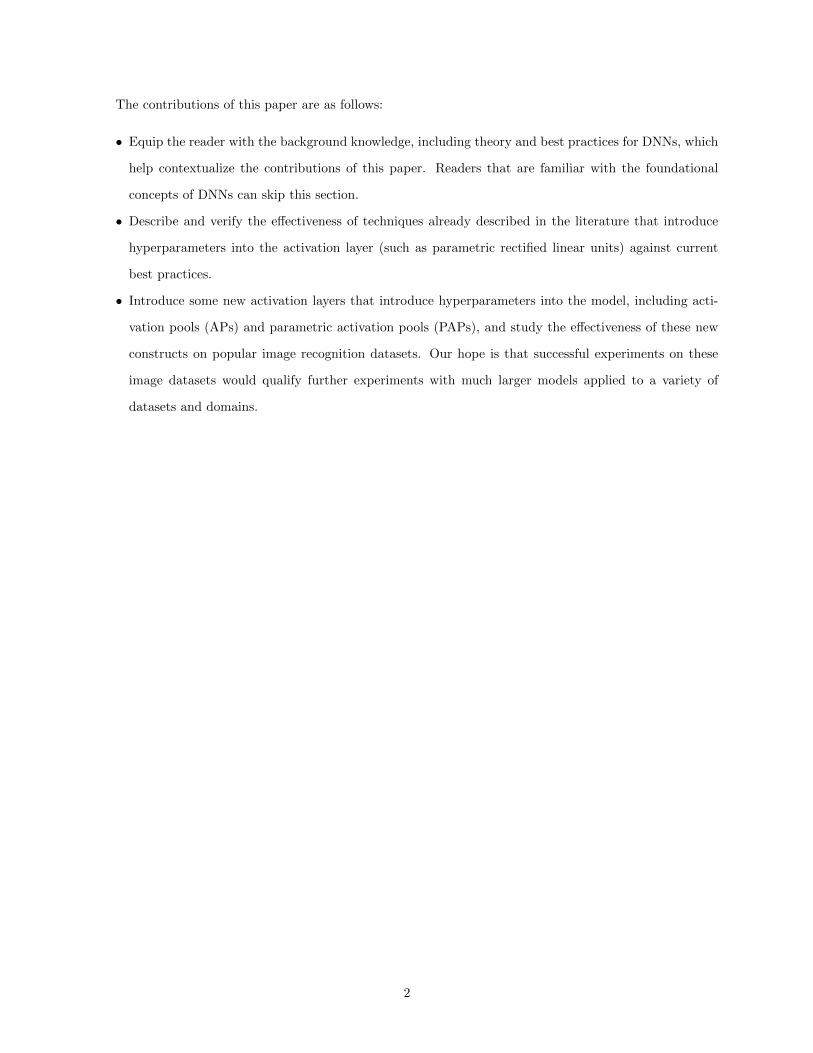
Figure 2: Example of a neural network with 3 layers.

4

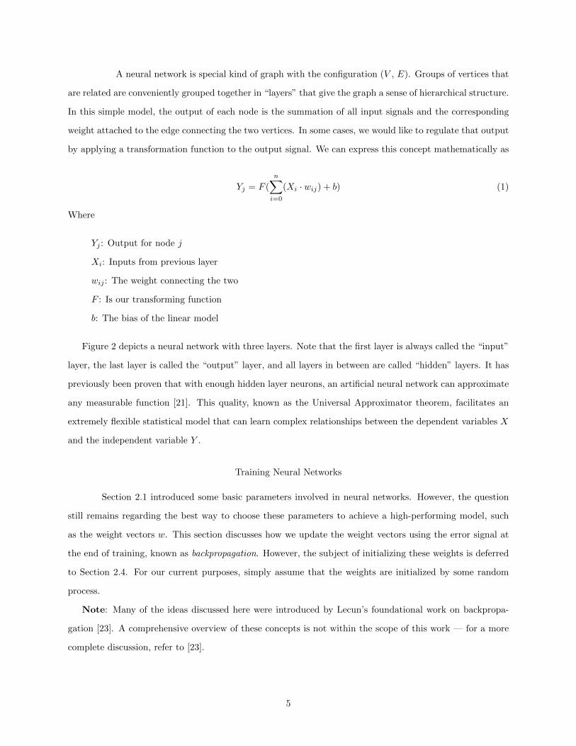
A neural network is special kind of graph with the configuration (V , E). Groups of vertices that

are related are conveniently grouped together in “layers” that give the graph a sense of hierarchical structure.

In this simple model, the output of each node is the summation of all input signals and the corresponding

weight attached to the edge connecting the two vertices. In some cases, we would like to regulate that output

by applying a transformation function to the output signal. We can express this concept mathematically as

Yj = F (

n∑i=0

(Xi · wij) + b) (1)

Where

Yj : Output for node j

Xi: Inputs from previous layer

wij : The weight connecting the two

F : Is our transforming function

b: The bias of the linear model

Figure 2 depicts a neural network with three layers. Note that the first layer is always called the “input”

layer, the last layer is called the “output” layer, and all layers in between are called “hidden” layers. It has

previously been proven that with enough hidden layer neurons, an artificial neural network can approximate

any measurable function [21]. This quality, known as the Universal Approximator theorem, facilitates an

extremely flexible statistical model that can learn complex relationships between the dependent variables X

and the independent variable Y .

Training Neural Networks

Section 2.1 introduced some basic parameters involved in neural networks. However, the question

still remains regarding the best way to choose these parameters to achieve a high-performing model, such

as the weight vectors w. This section discusses how we update the weight vectors using the error signal at

the end of training, known as backpropagation. However, the subject of initializing these weights is deferred

to Section 2.4. For our current purposes, simply assume that the weights are initialized by some random

process.

Note: Many of the ideas discussed here were introduced by Lecun’s foundational work on backpropa-

gation [23]. A comprehensive overview of these concepts is not within the scope of this work — for a more

complete discussion, refer to [23].

5

Backpropagation

The most common method for updating parameters in neural networks is through backpropagation.

Take, for instance, a neural network mapping function, defined as

Y = F(X) (2)

Where

X: Input

Y : Predicted output

F : NN mapping function

From this equation, we can derive a loss function which indicates how well our model currently fits the data.

There are many loss functions that could be used. However, the categorical cross-entropy function

(CCE) loss function is the most appropriate for the classification experiments in this paper. This loss function

quantifies the error in terms of misclassified datapoints, which is appropriate for our image classification tasks

in Section 4. This loss function is expressed mathematically as:

E = − 1

n

n∑i=1

[Yiln(Yi) + (1− Yi)ln(1− Yi)

](3)

Because a neural network is within the broader family of sequential graph-based structures, the output

of any given layer (notably, including the final output layer) Hi is a function of the state of the current layer

and all the output of the previous layer Hi−1 which depends on S1, · · · , Si−1. Thus, once error is computed,

we can compute the derivative of the loss function with the respect to the state of the n − 1 layer and its

input. Formally, we can express this as

∂E∂Si

=∂E

∂Hi−1· ∂Hi−1

∂S(4)

Keen observers will note that this derivation is simply the chain rule. The main takeaway is that, given

enough time, we can compute the derivative of the loss function with respect to every parameter of the

network through a process called backpropagation. These values can used to tune our model by adjusting

the parameters through an optimization function. Many optimization functions exist, however, this paper

will use the standard stochastic gradient descent algorithm which is expressed as

St = St−1 − η∂E

∂St−1(5)

6

Where

St: New configuration of the layer

St−1: Old configuration of the layer

η: learning rate (generally around 0.01)

An understanding of backpropagation is extremely important for the comprehension of the ideas intro-

duced in this paper, notably:

• Adding more trainable parameters to the model increasing the amount of variables which have to be

tuned in the model. This negatively impacts the amount of time it takes to train a neural network.

• Training a neural network through backpropagation is a balancing act. Adding more trainable param-

eters to the model can start to adversely affect performance if the parameters of the model cannot

converge, creating a curse of dimensionality effect. More parameters for backpropagation to balance

means it is more difficult for a network to converge.

• The selection of the learning rate η is crucial: if the learning rate is too low, the network takes too

long to train. If the learning rate is too high, the network “skips over” the best solution because it

is trying to cover too much ground each training iteration. The goal is to choose the highest possible

learning rate without adversely affecting performance. The ideas proposed in Section 3 are mainly to

increase the maximum learning rate.

Vanishing/Exploding Gradients

The introduction of gradient based learning into our network also introduces several potential prob-

lems, especially in Recurrent Neural Networks (RNNs) [14, 3, 30]. As the error is propagated backwards

from the last time-step towards the first time-step, the gradients can experience a drifting problem where the

gradients at the beginning of the network either grow or shrink exponentially. In this section, an attempt

will be made to convince the reader of the severity of vanishing and exploding gradients in RNNs.

Note: the following analysis is simplified for the purposes of this paper and loosely follows [30]. For a

more complete view of vanishing or exploding gradients, please refer to their fantastic work.

Consider the gradient for a recurrent neural network layer, expressed as

∂E∂Si

=∑

1≤t≤T

∂Et∂Si

(6)

For our purposes, it is sufficient to note that the computation of each term ∂EtSi

requires the error to be

backpropagated from the inputs 1→ t. For any given input, we can backpropagate the error by the equation

7

∂Xt

∂Xk=∏t≥i>k

∂Xi

∂Xi−1(7)

Here, the problem becomes obvious: as the gradients due to the inputs shift backwards in time, the

denominator of each term in this product can easily drive that term towards 0 or ∞, show by the equations

lim∂Xi−1→β

∂Xi

∂Xi−1=

0, when β =∞

∞, when β = 0

(8)

When you consider the product of these terms, it is clear that multiple terms can easily create a feedback

loop that pushes the value towards 0 or ∞. Furthermore, the magnitude of the problem increases as the

number of terms being multiplied increases. Thus, gradients for the earlier time-steps in RNNs can easily

be distorted. This phenomena caused researchers much trouble when modeling time series data of long

periods of time until the invention of the Long Short Term Memory (LSTM) [13] and Gated Recurrent

Unit (GRU) [7] layers. In Section 3, we propose some constructs that should decrease the potential for

vanishing/exploding gradients.

Activation Functions

In neural networks, an activation function is a squashing function that takes as its input the sum-

mation of all connected input signals and maps that value to a scaled output. This process is roughly related

to how human neurons work where some combination of input connections determines whether the neuron

should fire or not. Applying an activation function to the output of each layer normalizes the network and

helps prevent exploding weights in the network.

Sigmoid Activation Functions

A sigmoid function is a class of function that produces a sigmoid, or ‘S-shaped’ curve. Sigmoid

functions are good choices for squashing functions as they provide sufficient non-linearity to learn quickly

while treating very high or very-low values of x the same. Three common sigmoid functions are the logistic

function [23], the hyperbolic tangent function [23], and the softsign function [4] given by

8

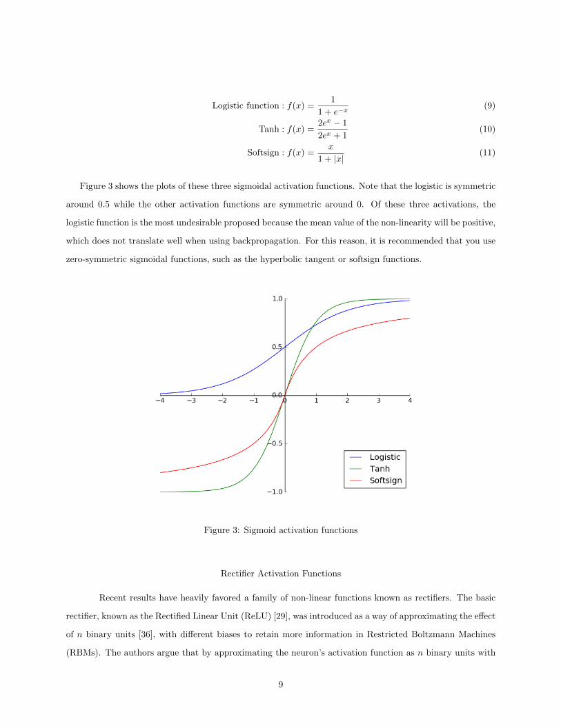
Logistic function : f(x) =1

1 + e−x(9)

Tanh : f(x) =2ex − 1

2ex + 1(10)

Softsign : f(x) =x

1 + |x|(11)

Figure 3 shows the plots of these three sigmoidal activation functions. Note that the logistic is symmetric

around 0.5 while the other activation functions are symmetric around 0. Of these three activations, the

logistic function is the most undesirable proposed because the mean value of the non-linearity will be positive,

which does not translate well when using backpropagation. For this reason, it is recommended that you use

zero-symmetric sigmoidal functions, such as the hyperbolic tangent or softsign functions.

Figure 3: Sigmoid activation functions

Rectifier Activation Functions

Recent results have heavily favored a family of non-linear functions known as rectifiers. The basic

rectifier, known as the Rectified Linear Unit (ReLU) [29], was introduced as a way of approximating the effect

of n binary units [36], with different biases to retain more information in Restricted Boltzmann Machines

(RBMs). The authors argue that by approximating the neuron’s activation function as n binary units with

9

different biases will operate more similarly to how neurons actually fire without increasing computational

complexity.

Another major benefit arising from ReLUs is that they tend to produce sparse networks [26]. The intuition

is that sparsity in neural networks is important for robustness — if the output of a neuron is non-zero, that

neuron’s parameters would be “tuned” by backpropagation. Thus, enforcing a structure where it is difficult

for the activation function to be close to zero is akin to saying that every input should affect every neuron

in the network. This idea is not consistent with our current understanding of the brain and, in fact, produces

worse results than sparse networks. Thus, sparsity is often viewed with favor by researchers, especially in

deeper neural networks where the problem is exacerbated with the growing number of neurons.

There are many different forms of rectifiers, such as the vanilla Rectified Linear Unit (ReLU) [29], the

Leaky Rectified Linear Unit (LReLU) [26], the Parametric Rectified Linear Unit (PReLU) [18], and the

Exponential Linear Unit (ELU) [10], which are given by

ReLU : f(x) =

x, if x > 0

0, otherwise

(12)

LReLU : f(x, α) =

x, if x > 0

αx, otherwise

(13)

PReLU : f(x, α) =

x, if x > 0

αx, otherwise

where α is trainable. (14)

ELU : f(x, α) =

x, if x > 0

α(ex − 1), otherwise

(15)

Figure 4 shows the output of these activation functions. Note that the functions for the LReLU and the

PReLU are the same. The different between these two functions is that the α parameter is a trainable part

of the network in the PReLU and a constant in the LReLU. All of these derivations have different benefits

in neural networks — different rectifiers work better on different types of data and even within the same

subject area! For our purposes, it is sufficient to recognize the benefits of rectifiers in general and to point

out the introduction of trainable parameters into the activation function, as is the case with the PReLU.

10

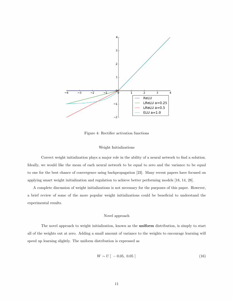
Figure 4: Rectifier activation functions

Weight Initializations

Correct weight initialization plays a major role in the ability of a neural network to find a solution.

Ideally, we would like the mean of each neural network to be equal to zero and the variance to be equal

to one for the best chance of convergence using backpropagation [23]. Many recent papers have focused on

applying smart weight initialization and regulation to achieve better performing models [18, 14, 28].

A complete discussion of weight initializations is not necessary for the purposes of this paper. However,

a brief review of some of the more popular weight initializations could be beneficial to understand the

experimental results.

Novel approach

The novel approach to weight initialization, known as the uniform distribution, is simply to start

all of the weights out at zero. Adding a small amount of variance to the weights to encourage learning will

speed up learning slightly. The uniform distribution is expressed as

W ∼ U [ − 0.05, 0.05 ] (16)

11

Lecun’s Distribution

Presented in [23, Sec 4.6], Lecun’s distribution assumes a linear model and is based on the following

argument: suppose we have a neural network activation layer that uses tanh(X) as a non-linear squashing

function. In order for convergence to occur quickly, the weights should be initialized so that (1) the weights

are not too small, causing the gradient function to be small and (2) the tanh is not saturated (the weights are

not too large), also causing the gradient function to be small. Assuming that the data is properly normalized,

all we need to do is initialize the weights to have µ = 0 and σ = 1. Thus, we can draw values from a uniform

random distribution that will give us these characteristics. Lecun’s distribution is expressed as

W ∼ U[− 1√nj,

1√nj

](17)

Glorot Normalized Distribution

The Glorot initialization was derived in [14, 4.2]. Building on research presented in [6], the authors

attempt to derive an activation function that keeps data flowing through all layers of the deep neural network

while avoiding exploding and vanishing gradients [3]. By asserting that the activation functions be linear

and making some reasonable assumptions about the nature of the network, the authors arrive at the function

W ∼ U

[−

√6

√nj + nj+1

,

√6

√nj + nj+1

](18)

For a full analysis, please refer to the paper listed above.

He Distribution

By 2014, the trend in the literature has changed from activation functions such as the sigmoid and

softplus activation functions to ReLUs [18][pg. 4]. All previous initializations assumed a linear activation

function, which is not suitable for ReLU or its variations. Thus, the authors of derive a theoretically sound

initialization for networks utilizing the ReLU activation family, given as

W ∼ U

[−

√6

nj,

√6

nj

](19)

For a full analysis, please refer to the paper listed above.

12

CHAPTER 3

THEORETICAL CONCEPTS

PReLUs (introduced in Section 2.3) are the first known example of introducing hyperparameters into

the activation function layer that we are aware of. Here, the hyperparameter α (the slope of the negative

part) is included as a trainable parameter of the network. By including this trainable parameter in the

model, the authors achieved significant performance improvements over the standard ReLU networks while,

at the same time, surpassing human-level recognition of objects in an image recognition task [18]. These

results certainly warrant further investigation into trainable activation functions. Thus, we introduce the

concept of activation pools (APs) and parametric activation pools (PAPs).

Activation Pools

The intuition behind an activation pool is simple: instead of transforming an input signal by one

activation function, we

1. Split the incoming signal by a some coefficient.

2. Push the scaled signal through multiple activation functions.

3. Merge the signal back together by summing the signals.

This system can be viewed as a voting system where different activation functions get to vote on the

what the output value should be. Figure 5 illustrates the architecture of an activation pool.

In activation pools, the branching factor αi is a constant that is not a trainable parameter of the network.

Conversely, the parametric activation pool introduces the branching factor α as a trainable parameter for the

model. However, it is generally not wise to allow the branching factors to range from (−∞,∞), as adding

multiple activation functions could combine exponentially to explode your network. Therefore, the following

two constraints are suggested:

13

Figure 5: Architecture for activation pools

14

• Threshold: A threshold is applied for each branching factor αi such that αij = max(min(αi0, αij),−αi0)

where αij is the branching factor at time-step j and αi0 is the branching factor of αi at initialization.

The guarantees that αi ∈ [−αi0, αi0] at any time-step.

• Scaling factor: For more constricted cases, we can enforce that the sum of the branching factors is

1. E.g.i∑αi = 1. In our experiments, we achieve this by using thresholding.

Momentum

The architecture of activation pools allows for some very interesting combinations of activation func-

tions. One particularly interesting concept is the idea of adding momentum to an activation function. This

construct, inspired by a proportional—integral—derivative controller (PID controller) in electrical engineer-

ing, can be conceptualized as incorporating past errors (the derivative signal) and future expected errors

(the integral signal) into the equation.

Momentum for ReLU

This idea becomes clear when examining a particular activation function. Take for instance a

standard implementation of ReLU (Section 2.3). Loosely speaking, we can represent the PID functions for

ReLU as follows:

Derivative : f(x) =

1, if x > 0

0, otherwise

(20)

Proportional : f(x) =

x, if x > 0

0, otherwise

(21)

Integral : f(x) =

x2

2 , if x > 0

0, otherwise

(22)

(23)

In many cases (including case of the ReLU), the integral signal is not suitable for use in neural networks

— applying the input by an exponential factor could quickly cause some weight vectors to explode, leading to

instability in the network. Thus, we will refer to a Momentum ReLU as only the proportional and derivative

signals of a ReLU activation function.

15

The relationship between the ReLU and the derivative signal (a step function) can be expressed in a more

intuitive way: suppose we have a Momentum ReLU with the constraint that all of the branching coefficients

must sum to 1. When all of the signal is flowing through the ReLU branch and none of the signal flowing

through the step function branch, the Momentum ReLU acts exactly as a standard ReLU. Increasing the

amount of signal that flows to the step function, however, will proportionally decrease the amount of signal

flowing to the ReLU. Since the step function is simply a constant value, it will not add any gradient with

respect to the cost function when training by backpropagation. Thus, adding more signal to the step function

is equivalent to reducing the amount of gradient the ReLU branch can contribute in the training process.

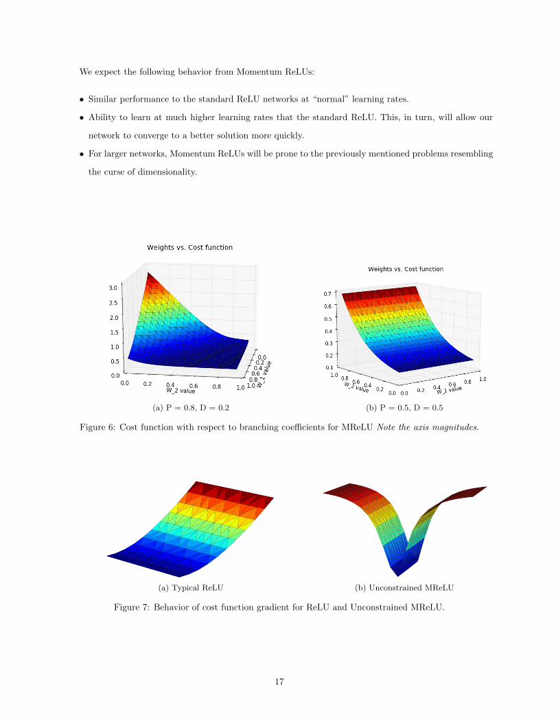
Concretely, as more of the signal flows to the step function instead of to the ReLU, the gradient surface with

respect to the cost function can become smoother. This phenomena is easily verified empirically and shown

in Figure 6.

By relaxing the constraint that the branching coefficients must sum to 1, we can also achieve some

interesting results. Unconstrained Momentum ReLUs are also able to find clearly defined local minima

as shown in Figure 7. This is primarily because the network can compound the ReLU signal by a linear

factor (namely, the branching coefficient which is now unbounded). However, this behavior may desired or

undesired behavior depending on your application and network design.

From this analysis, it is clear that adding momentum to the ReLU activation function produces several

interesting characteristics, including both theoretical (the ability for the backpropagation to maintain some

idea of where the training error has been in the past) and practical (the ability of the network to tweak

the slope of the activation layer’s cost gradient) nuances. As always, there are some trade-offs to consider

when introducing more trainable parameters into your model, such as computational complexity and the

potential curse of dimensionality. However, these detriments are easy to estimate and depend on your specific

implementation.

16

We expect the following behavior from Momentum ReLUs:

• Similar performance to the standard ReLU networks at “normal” learning rates.

• Ability to learn at much higher learning rates that the standard ReLU. This, in turn, will allow our

network to converge to a better solution more quickly.

• For larger networks, Momentum ReLUs will be prone to the previously mentioned problems resembling

the curse of dimensionality.

(a) P = 0.8, D = 0.2 (b) P = 0.5, D = 0.5

Figure 6: Cost function with respect to branching coefficients for MReLU Note the axis magnitudes.

(a) Typical ReLU (b) Unconstrained MReLU

Figure 7: Behavior of cost function gradient for ReLU and Unconstrained MReLU.

17

CHAPTER 4

EXPERIMENTS

All of the following experiments are trained on a single NVIDIA Tesla K20m GPU in the Mississippi

Center for Supercomputing Research’s GPU cluster using the popular deep learning libraries Theano and

Keras. All models are trained using Nesterov-flavored stochastic gradient descent with a weight decay of

1e−6 and a momentum factor of 0.9. Weight initializations are used appropriately as described in Section

2.4. All sources and results can be found on Github 1.

MNIST Classification

We first evaluate our new activation constructs on the MNIST training dataset2 to create a baseline

for performance and to motivate further experiments. The MNIST dataset is an image classification dataset

that is comprised of 28x28x1 images of handwritten digits [0..9]. The models are trained and validated on

the 60,000 training images then tested on the 10,000 testing images. The primary goal of this experiment us

to compare the performance of the activation layers presented against the standard ReLU activation layers

in the same model, not to achieve world-class results. Thus, no image preprocessing is performed and very

little thought was given to the tuning of the model itself.

Standard Model. The standard model consists of shallow, fully-connected (FC) building blocks with

dropout to prevent overfitting [33]. The only difference between the architectures tested was the activation

layer following each FC layer in the model. Since even simple models can achieve high accuracy quickly on

the MNIST training set, only two building blocks with 512 FC nodes each are needed. Table 1 shows the

model architectures for each activation layer tested.

1http://github.com/claymcleod/pap-experiment2http://yann.lecun.com/exdb/mnist/

18

layer name output dim ReLU PReLU MReLU MReLU (threshold)

FC 1 512 FCx512

AC 1 512 relu prelu mrelu mrelu-t

DO 1 512 20% dropout

FC 2 512 FCx512

AC 2 512 relu prelu mrelu mrelu-t

DO 2 512 20% dropout

output 10 FCx10 and softmax

Table 1: Model architectures for MNIST experiment. Note that the activation layers are different for eachmodel tested.

19

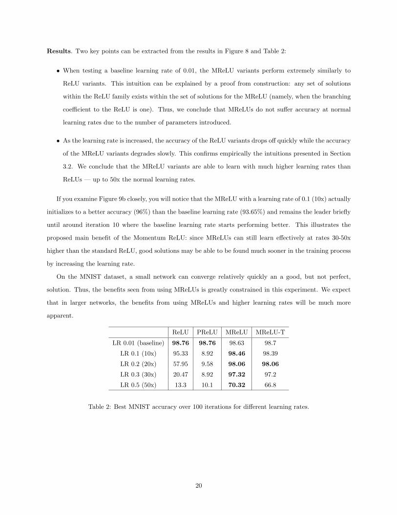
Results. Two key points can be extracted from the results in Figure 8 and Table 2:

• When testing a baseline learning rate of 0.01, the MReLU variants perform extremely similarly to

ReLU variants. This intuition can be explained by a proof from construction: any set of solutions

within the ReLU family exists within the set of solutions for the MReLU (namely, when the branching

coefficient to the ReLU is one). Thus, we conclude that MReLUs do not suffer accuracy at normal

learning rates due to the number of parameters introduced.

• As the learning rate is increased, the accuracy of the ReLU variants drops off quickly while the accuracy

of the MReLU variants degrades slowly. This confirms empirically the intuitions presented in Section

3.2. We conclude that the MReLU variants are able to learn with much higher learning rates than

ReLUs — up to 50x the normal learning rates.

If you examine Figure 9b closely, you will notice that the MReLU with a learning rate of 0.1 (10x) actually

initializes to a better accuracy (96%) than the baseline learning rate (93.65%) and remains the leader briefly

until around iteration 10 where the baseline learning rate starts performing better. This illustrates the

proposed main benefit of the Momentum ReLU: since MReLUs can still learn effectively at rates 30-50x

higher than the standard ReLU, good solutions may be able to be found much sooner in the training process

by increasing the learning rate.

On the MNIST dataset, a small network can converge relatively quickly an a good, but not perfect,

solution. Thus, the benefits seen from using MReLUs is greatly constrained in this experiment. We expect

that in larger networks, the benefits from using MReLUs and higher learning rates will be much more

apparent.

ReLU PReLU MReLU MReLU-T

LR 0.01 (baseline) 98.76 98.76 98.63 98.7

LR 0.1 (10x) 95.33 8.92 98.46 98.39

LR 0.2 (20x) 57.95 9.58 98.06 98.06

LR 0.3 (30x) 20.47 8.92 97.32 97.2

LR 0.5 (50x) 13.3 10.1 70.32 66.8

Table 2: Best MNIST accuracy over 100 iterations for different learning rates.

20

(a) ReLU/PReLU results for different learning rates using the Standard architecture for MNIST.

(b) MReLU/MReLU (threshold) results for different learning rates using the Standard architecturefor MNIST.

Figure 8: MNIST accuracy for different learning rates.

21

CIFAR10

Next, we test these constructs against the more challenging CIFAR10 dataset3. CIFAR10 is an image

classification dataset that is comprised of 32x32x3 color images of 10 different classes of objects, where each

pixel has a red, a blue, and a green channel. Expanding the images from black and white to color presents a

chance to create many more interesting convolutional filters, so the network takes longer to converge. Thus,

the CIFAR10 dataset is appropriate for comparing the performance and convergence of different activation

layers in the same network.

In this experiment, the models are trained and validated on the 50,000 training images then tested on

the 10,000 testing images. Now that the basis for further exploration has been established, we will examine

the effects of the activation layers proposed in this paper against standard ReLU activation layers in more

complex networks and datasets. No image preprocessing is performed and very little thought was given to

the tuning of the model itself.

DeepCNet Model. Currently, the best reported results that we are aware of for the CIFAR10 dataset

achieved 96.53% accuracy through heavy data augmentation, fractional max-pooling, and a model known as a

DeepCNet [16]. DeepCNets (introduced in [17]) use many stacks of convolutional layers and 2x2 max-pooling

to retain spatial information effectively. However, this slow max-pooling technique means DeepCNets require

a significant number of layers to encapsulate all of the information in an image, which leads to relatively slow

convergence. Combined with the ability to learn at much higher learning rates from our proposed activation

layers, we expect both the performance and the convergence time of the DeepCNet to improve.

The model presented is relatively small compared to other DeepCNets due to memory constraints of

our GPU. As with the last experiment, the only difference between the different models tested are the ac-

tivation layers utilized. For those familiar with the DeepCNet notation, the model used is denoted as a

DeepCNet(5, 25) with an additional C1 at the end of the model. A dropout of 20% was used to prevent

overfitting [33]. Techniques such as data augmentation and batch normalization were not used, since we

were not attempting to achieve world class results. Table 3 shows the model architectures for each activation

layer tested.

Preliminary Experiments. Before we can test the absolute performance of each of the activation layers,

we first need to have some intuition about the highest learning rate which each activation layer can learn a

statistical mapping. This experiment also serves as a general confirmation that Momentum ReLUs can learn

3https://www.cs.toronto.edu/ kriz/cifar.html

22

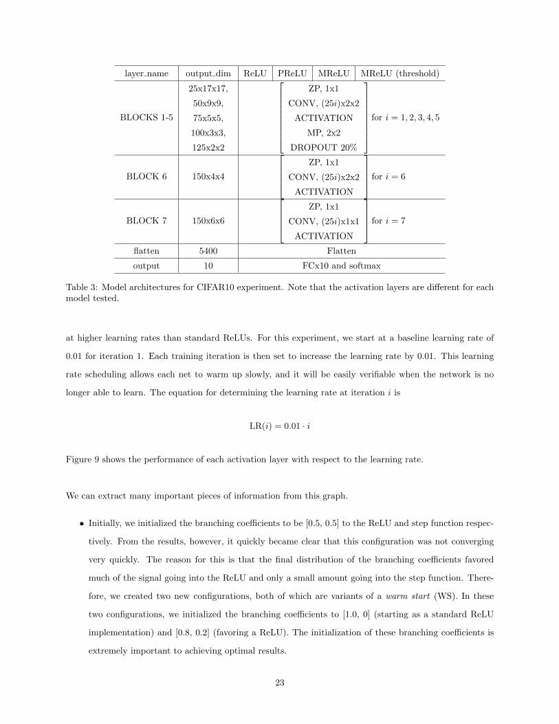
layer name output dim ReLU PReLU MReLU MReLU (threshold)

BLOCKS 1-5

25x17x17,

50x9x9,

75x5x5,

100x3x3,

125x2x2

ZP, 1x1

CONV, (25i)x2x2

ACTIVATION

MP, 2x2

DROPOUT 20%

for i = 1, 2, 3, 4, 5

BLOCK 6 150x4x4

ZP, 1x1

CONV, (25i)x2x2

ACTIVATION

for i = 6

BLOCK 7 150x6x6

ZP, 1x1

CONV, (25i)x1x1

ACTIVATION

for i = 7

flatten 5400 Flatten

output 10 FCx10 and softmax

Table 3: Model architectures for CIFAR10 experiment. Note that the activation layers are different for eachmodel tested.

at higher learning rates than standard ReLUs. For this experiment, we start at a baseline learning rate of

0.01 for iteration 1. Each training iteration is then set to increase the learning rate by 0.01. This learning

rate scheduling allows each net to warm up slowly, and it will be easily verifiable when the network is no

longer able to learn. The equation for determining the learning rate at iteration i is

LR(i) = 0.01 · i

Figure 9 shows the performance of each activation layer with respect to the learning rate.

We can extract many important pieces of information from this graph.

• Initially, we initialized the branching coefficients to be [0.5, 0.5] to the ReLU and step function respec-

tively. From the results, however, it quickly became clear that this configuration was not converging

very quickly. The reason for this is that the final distribution of the branching coefficients favored

much of the signal going into the ReLU and only a small amount going into the step function. There-

fore, we created two new configurations, both of which are variants of a warm start (WS). In these

two configurations, we initialized the branching coefficients to [1.0, 0] (starting as a standard ReLU

implementation) and [0.8, 0.2] (favoring a ReLU). The initialization of these branching coefficients is

extremely important to achieving optimal results.

23

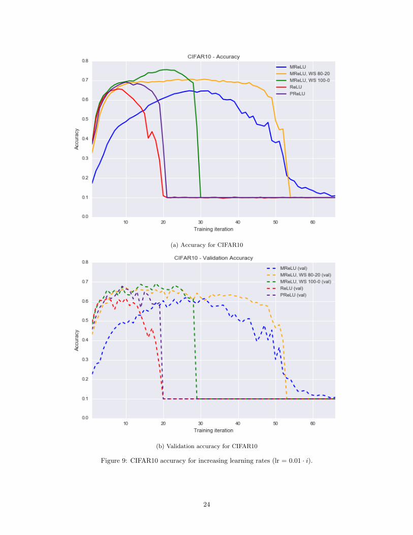
(a) Accuracy for CIFAR10

(b) Validation accuracy for CIFAR10

Figure 9: CIFAR10 accuracy for increasing learning rates (lr = 0.01 · i).

24

• As you can see from the graph, each flavor of the MReLU has it’s own advantages: it is clear that the

initialization of the branching coefficients is a tradeoff between performance and learnability.

– A configuration of [1.0, 0.0] achieves the highest accuracy, but sacrifices learnability at higher

learning rates.

– A configuration of [0.5, 0.5] continues to learn for the longest amount of time, but it achieves the

lowest accuracy.

– A configuration of [0.8, 0.2] most resembles to desired distribution of the branching coefficients.

We found that this configuration was a good balance between the two, as high accuracy and

learnability were both achieved.

• Every MReLU configuration achieves similar or better accuracy than the standard ReLU/PReLU while

retaining much higher learnability.

• The PReLU does, in fact, outperform the standard ReLU in both accuracy and learnability as described

in [18].

Constant LR Experiments. Now that we have established a range of reasonable learning rates for each

activation function, it would be useful to understand how each activation function reacts for constant learning

rates. Table 4 shows the accuracy for each activation function tested at different constant learning rates

and the training iteration that accuracy was achieved (in parenthesis). This results of this experiment yield

several interesting results:

• The standard MReLU implementation with [0.5, 0.5] branching factor learns much slower than the

other implementations. Note that most of the MReLU’s reach their maximum accuracy at the last

training iteration, meaning that it is continuing to learn all the way until the last iteration. More

training iterations might improve the improve the maximum accuracy scores for the MReLU.

• Conversely, the MReLUs that are initialized with a [0.8, 0.2] branching factor generally outperform

the standard ReLUs.

• PReLUs consistenly match or outperform all of the implementations, confirming the findings of [18].

The results of this experiment seem puzzling at first: the PReLU implementations perform relatively poorly

with dynamic learning rates but outperform all of the other activation layers tried with constant learning

rates. It seems, therefore, that to take advantage of the Momentum-based activation functions, we should

build some dynamic based learning rate experiment with optimal learning rates to test whether or not

MReLU variants can yield better results.

25

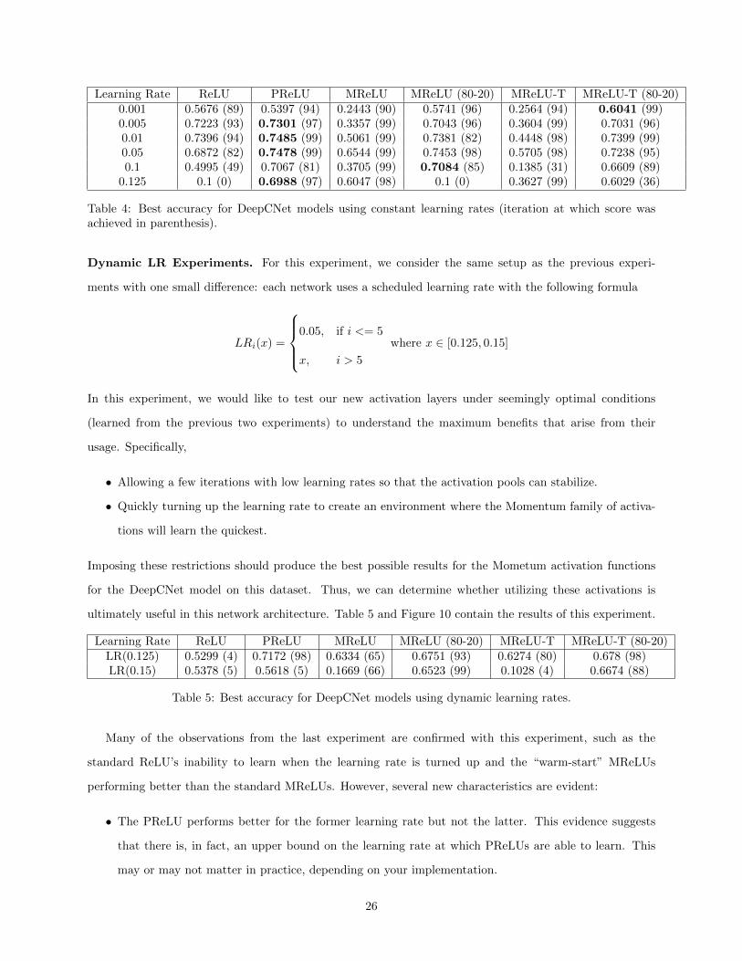
Learning Rate ReLU PReLU MReLU MReLU (80-20) MReLU-T MReLU-T (80-20)0.001 0.5676 (89) 0.5397 (94) 0.2443 (90) 0.5741 (96) 0.2564 (94) 0.6041 (99)0.005 0.7223 (93) 0.7301 (97) 0.3357 (99) 0.7043 (96) 0.3604 (99) 0.7031 (96)0.01 0.7396 (94) 0.7485 (99) 0.5061 (99) 0.7381 (82) 0.4448 (98) 0.7399 (99)0.05 0.6872 (82) 0.7478 (99) 0.6544 (99) 0.7453 (98) 0.5705 (98) 0.7238 (95)0.1 0.4995 (49) 0.7067 (81) 0.3705 (99) 0.7084 (85) 0.1385 (31) 0.6609 (89)

0.125 0.1 (0) 0.6988 (97) 0.6047 (98) 0.1 (0) 0.3627 (99) 0.6029 (36)

Table 4: Best accuracy for DeepCNet models using constant learning rates (iteration at which score wasachieved in parenthesis).

Dynamic LR Experiments. For this experiment, we consider the same setup as the previous experi-

ments with one small difference: each network uses a scheduled learning rate with the following formula

LRi(x) =

0.05, if i <= 5

x, i > 5

where x ∈ [0.125, 0.15]

In this experiment, we would like to test our new activation layers under seemingly optimal conditions

(learned from the previous two experiments) to understand the maximum benefits that arise from their

usage. Specifically,

• Allowing a few iterations with low learning rates so that the activation pools can stabilize.

• Quickly turning up the learning rate to create an environment where the Momentum family of activa-

tions will learn the quickest.

Imposing these restrictions should produce the best possible results for the Mometum activation functions

for the DeepCNet model on this dataset. Thus, we can determine whether utilizing these activations is

ultimately useful in this network architecture. Table 5 and Figure 10 contain the results of this experiment.

Learning Rate ReLU PReLU MReLU MReLU (80-20) MReLU-T MReLU-T (80-20)LR(0.125) 0.5299 (4) 0.7172 (98) 0.6334 (65) 0.6751 (93) 0.6274 (80) 0.678 (98)LR(0.15) 0.5378 (5) 0.5618 (5) 0.1669 (66) 0.6523 (99) 0.1028 (4) 0.6674 (88)

Table 5: Best accuracy for DeepCNet models using dynamic learning rates.

Many of the observations from the last experiment are confirmed with this experiment, such as the

standard ReLU’s inability to learn when the learning rate is turned up and the “warm-start” MReLUs

performing better than the standard MReLUs. However, several new characteristics are evident:

• The PReLU performs better for the former learning rate but not the latter. This evidence suggests

that there is, in fact, an upper bound on the learning rate at which PReLUs are able to learn. This

may or may not matter in practice, depending on your implementation.

26

(a) Accuracy for CIFAR10 with dynamic learning rate

(b) Validation accuracy for CIFAR10 with dynamic learning rate

Figure 10: CIFAR10 accuracy for dynamic learning rates.

27

• As with the last experiment, MReLUs with a “warm-start” perform better in general than standard

MReLUs. However, standard MReLUs also appear to have an upper bound on the learning rates at

which they are able to learn, as seen by their poor performance at the higher learning rate. “Warm-

start” MReLUs continue to perform well at both learning rates.

Despite these results, ultimately our optimal environment did not produce better accuracy rates in the

same amount of iterations than the results in Table 4 at much lower learning rates. Thus, the new activation

layers are not currently a viable alternative to PReLUs for this network architecture and dataset.

28

CHAPTER 5

FURTHER WORK/CONCLUSION

While the accuracy did not improve using the DeepCNet architecture on the CIFAR10 dataset,

several important benefits of Mometum ReLUs and activation pools in general were observed. In fact,

there are several directions that could not be covered in this paper that might realize the potential of these

constructs.

Datasets

Tackling the CIFAR10 dataset with large number of parameters was an ambituous goal. PReLUs

have been firmly established as best practice on many image recognition datasets, including the CIFAR10

dataset [18, 17]. We suspect that the reason for this is that PReLUs provide a moderate level of variability

while maintaining stability for deep models: as you increase the number of trainable parameters, the curse

of dimensionality diminishes any returns you might gain from increased flexibility.

However, the results on the MNIST dataset (Section 4.1) suggest that PReLUs do not work well for all

image recognition datasets at high learning rates. In fact, PReLUs are not generally used (to our knowledge)

in practice outside of the image recognition domain. Conversely, the Momentum ReLU variant generally

outperforms a standard ReLU on all datasets. Thus, applying MReLUs to different datasets might yield

vastly improved results over the standard ReLU.

Models

As noted in Section 5.1, we believe that much of the shortcomings of the Momentum ReLU variants

for the CIFAR10 dataset is due to the curse of dimensionality. Deeper models are often preferred when

classifying image data because of their ability to construct a hierarchical set of features exploiting spatial

characteristics. Since we did not anticipate the strong effect of the curse of dimensionality, we selected a

relatively deep architecture for our model that performed well on similar image recognition tasks. From

Section 4.1, it is clear that Momentum ReLU variants perform better in shallow architectures than in deeper

architectures. Thus, we submit that these ideas applied to much shallower models might be more successful.

29

Activation Pools

While we believe that the ideas submitted for momentum-based activation pools might be useful

in practice, they are certainly not the only way to benefit from the use of activation pools. Many other

combinations of activation functions (with both constant and dynamic branching parameters) might be

useful for different domains. In general, we encourage the reader to pursue activation functions that produce

cost functions with a balance of smoothness and steepness. This, in turn, will allow gradient descent to (a)

converge the quickest and (b) have the most likely chance of consistently finding a global minimum.

Conclusion

This paper examines the performance of hyperparameters in activation layers for deep neural net-

works. The primary contribution of this paper is the introduction of activation pools and, specifically, the

concept of momentum in activation functions, as a possible useful construct for training at higher learning

rates. The performance of these activation functions were compared against standard ReLU implementations,

as well as other activation functions containing hyperparameters (namely, the parametric ReLU).

We find that the results suggest that momentum-based ReLUs can continue to learn at higher learning

rates across many network architectures and datasets compared to standard activation functions. However,

expectations should be tempered because this ability does not necessarily increase performance, either more

quickly or absolutely, for large network architectures. We believe that this outcome can primarily be at-

tributed to the curse of dimensionality — as one adds more trainable parameters to the model, it becomes

much harder for the weights to stabilize towards a global solution. However, we expect these momentum-

based models to consistently outperform standard activation functions in shallower networks across most

datasets.

30

BIBLIOGRAPHY

31

[1] Deep learning: does reality match the hype? Available at http://vote.sparklit.com/poll.spark/203792.

[2] How convolutional neural networks see the world. Available at http://blog.keras.io/how-convolutional-

neural-networks-see-the-world.html.

[3] Bengio, Y., Simard, P., and Frasconi, P. Learning long-term dependencies with gradient descent

is difficult. Neural Networks, IEEE Transactions on 5, 2 (1994), 157–166.

[4] Bergstra, J., Desjardins, G., Lamblin, P., and Bengio, Y. Quadratic polynomials learn bet-

ter image features. Tech. rep., Technical Report 1337, Departement dInformatique et de Recherche

Operationnelle, Universite de Montreal, 2009.

[5] Bordes, A., Chopra, S., and Weston, J. Question answering with subgraph embeddings. arXiv

preprint arXiv:1406.3676 (2014).

[6] Bradley, D. M. Learning in modular systems. Tech. rep., DTIC Document, 2010.

[7] Cho, K., van Merrienboer, B., Bahdanau, D., and Bengio, Y. On the properties of neural

machine translation: Encoder-decoder approaches. arXiv preprint arXiv:1409.1259 (2014).

[8] Cho, S. J. K., Memisevic, R., and Bengio, Y. On using very large target vocabulary for neural

machine translation.

[9] Ciodaro, T., Deva, D., De Seixas, J., and Damazio, D. Online particle detection with neural

networks based on topological calorimetry information. In Journal of Physics: Conference Series (2012),

vol. 368, IOP Publishing, p. 012030.

[10] Clevert, D.-A., Unterthiner, T., and Hochreiter, S. Fast and accurate deep network learning

by exponential linear units (elus). arXiv preprint arXiv:1511.07289 (2015).

[11] Collobert, R., Weston, J., Bottou, L., Karlen, M., Kavukcuoglu, K., and Kuksa, P.

Natural language processing (almost) from scratch. The Journal of Machine Learning Research 12

(2011), 2493–2537.

[12] Farabet, C., Couprie, C., Najman, L., and LeCun, Y. Learning hierarchical features for scene

labeling. Pattern Analysis and Machine Intelligence, IEEE Transactions on 35, 8 (2013), 1915–1929.

[13] Gers, F. A., Schmidhuber, J., and Cummins, F. Learning to forget: Continual prediction with

lstm. Neural computation 12, 10 (2000), 2451–2471.

32

[14] Glorot, X., and Bengio, Y. Understanding the difficulty of training deep feedforward neural net-

works. In International conference on artificial intelligence and statistics (2010), pp. 249–256.

[15] Goodfellow, I. J., Shlens, J., and Szegedy, C. Explaining and harnessing adversarial examples.

arXiv preprint arXiv:1412.6572 (2014).

[16] Graham, B. Fractional max-pooling. arXiv preprint arXiv:1412.6071 (2014).

[17] Graham, B. Spatially-sparse convolutional neural networks. arXiv preprint arXiv:1409.6070 (2014).

[18] He, K., Zhang, X., Ren, S., and Sun, J. Delving deep into rectifiers: Surpassing human-level per-

formance on imagenet classification. In Proceedings of the IEEE International Conference on Computer

Vision (2015), pp. 1026–1034.

[19] Helmstaedter, M., Briggman, K. L., Turaga, S. C., Jain, V., Seung, H. S., and Denk, W.

Connectomic reconstruction of the inner plexiform layer in the mouse retina. Nature 500, 7461 (2013),

168–174.

[20] Hinton, G., Deng, L., Yu, D., Dahl, G. E., Mohamed, A.-r., Jaitly, N., Senior, A., Van-

houcke, V., Nguyen, P., Sainath, T. N., et al. Deep neural networks for acoustic modeling in

speech recognition: The shared views of four research groups. Signal Processing Magazine, IEEE 29, 6

(2012), 82–97.

[21] Hornik, K., Stinchcombe, M., and White, H. Multilayer feedforward networks are universal

approximators. Neural networks 2, 5 (1989), 359–366.

[22] Krizhevsky, A., Sutskever, I., and Hinton, G. E. Imagenet classification with deep convolutional

neural networks. In Advances in neural information processing systems (2012), pp. 1097–1105.

[23] LeCun, Y. A., Bottou, L., Orr, G. B., and Muller, K.-R. Efficient backprop. In Neural

networks: Tricks of the trade. Springer, 2012, pp. 9–48.

[24] Leung, M. K., Xiong, H. Y., Lee, L. J., and Frey, B. J. Deep learning of the tissue-regulated

splicing code. Bioinformatics 30, 12 (2014), i121–i129.

[25] Ma, J., Sheridan, R. P., Liaw, A., Dahl, G. E., and Svetnik, V. Deep neural nets as a method

for quantitative structure–activity relationships. Journal of chemical information and modeling 55, 2

(2015), 263–274.

[26] Maas, A. L., Hannun, A. Y., and Ng, A. Y. Rectifier nonlinearities improve neural network

acoustic models. In Proc. ICML (2013), vol. 30, p. 1.

33

[27] Mikolov, T., Deoras, A., Povey, D., Burget, L., and Cernocky, J. Strategies for training large

scale neural network language models. In Automatic Speech Recognition and Understanding (ASRU),

2011 IEEE Workshop on (2011), IEEE, pp. 196–201.

[28] Mishkin, D., and Matas, J. All you need is a good init. arXiv preprint arXiv:1511.06422 (2015).

[29] Nair, V., and Hinton, G. E. Rectified linear units improve restricted boltzmann machines. In

Proceedings of the 27th International Conference on Machine Learning (ICML-10) (2010), pp. 807–814.

[30] Pascanu, R., Mikolov, T., and Bengio, Y. On the difficulty of training recurrent neural networks.

arXiv preprint arXiv:1211.5063 (2012).

[31] Sainath, T. N., Mohamed, A.-r., Kingsbury, B., and Ramabhadran, B. Deep convolutional

neural networks for lvcsr. In Acoustics, Speech and Signal Processing (ICASSP), 2013 IEEE Interna-

tional Conference on (2013), IEEE, pp. 8614–8618.

[32] Schmidhuber, J. Deep learning in neural networks: An overview. Neural Networks 61 (2015), 85–117.

[33] Srivastava, N., Hinton, G., Krizhevsky, A., Sutskever, I., and Salakhutdinov, R. Dropout:

A simple way to prevent neural networks from overfitting. The Journal of Machine Learning Research

15, 1 (2014), 1929–1958.

[34] Sutskever, I., Vinyals, O., and Le, Q. V. Sequence to sequence learning with neural networks. In

Advances in neural information processing systems (2014), pp. 3104–3112.

[35] Szegedy, C., Liu, W., Jia, Y., Sermanet, P., Reed, S., Anguelov, D., Erhan, D., Van-

houcke, V., and Rabinovich, A. Going deeper with convolutions. In Proceedings of the IEEE

Conference on Computer Vision and Pattern Recognition (2015), pp. 1–9.

[36] Teh, Y. W., and Hinton, G. E. Rate-coded restricted boltzmann machines for face recognition.

Advances in neural information processing systems (2001), 908–914.

[37] Tompson, J. J., Jain, A., LeCun, Y., and Bregler, C. Joint training of a convolutional network

and a graphical model for human pose estimation. In Advances in neural information processing systems

(2014), pp. 1799–1807.

[38] Xiong, H. Y., Alipanahi, B., Lee, L. J., Bretschneider, H., Merico, D., Yuen, R. K., Hua,

Y., Gueroussov, S., Najafabadi, H. S., Hughes, T. R., et al. The human splicing code reveals

new insights into the genetic determinants of disease. Science 347, 6218 (2015), 1254806.

34