THE EFFECT OF MACROECONOMIC VARIABLES ON PORTFOLIO

RETURNS OF THE PENSION INDUSTRY IN KENYA

ELIZABETH WANJIKU

D63/79427/2012

A RESEARCH PROJECT SUBMITTED IN PARTIAL FULFILMENT

OF THE REQUIREMENTS FOR THE AWARD OF THE DEGREE OF

MASTER OF FINANCE, SCHOOL OF BUSINESS, UNIVERSITY OF

NAIROBI,

OCTOBER 2014

ii

DECLARATION

I, Elizabeth Wanjiku, do hereby declare that this research proposal is my original work and

has not been presented for a degree in any other University

Signed;

Elizabeth Wanjiku ……………………………….. Date………………………………

D63/79427/2012

This research project has been submitted for examination with my approval as the University

Supervisor.

Mr. Herick Ondigo

Lecturer,

Department of Finance and Accounting

School of Business,

University of Nairobi

Signed………………………………. Date……………………………….

iii

ACKNOWLEDGEMENTS

I am grateful to the Almighty God for his love mercy and protection. It is the Lord’s grace

that has brought me this far. We make plans but the Lord crowns them.

I wish to acknowledge, with gratitude the contribution of my supervisor Mr. Herrick Ondigo

who tirelessly guided me through the whole process, his patience in reading, correcting errors

and making suggestions for further improvement have enabled me to successfully complete

this project. I also wish to express my gratitude is extended to Mr. Cyrus Iraya who

moderated this document and whose comments were also source of improvement.

I also acknowledge the significant contribution of my lecturers who provided encouragement

and mentorship over the last two years. I thank my colleagues for their support, input and

suggestions. I wish to thank also my classmates and friends for their encouragement through

the course period.

My sincere gratitude to my family and friends for their unfailing support especially their

continued prayers, care and encouragement throughout the course.

Finally, I wish to thank all not mentioned above, but who in one way or another have

contributed to the success of this project through spiritual, moral and material support.

iv

DEDICATION

This dissertation is dedicated to my mother, for her unwavering love, good counsel care and

support.

v

TABLE OF CONTENTS

DECLARATION......................................................................................................................................... ii

ACKNOWLEDGEMENTS ...................................................................................................................... iii

DEDICATION............................................................................................................................................ iv

LIST OF TABLES ...................................................................................................................................... v

LIST OF FIGURES ................................................................................................................................. viii

LIST OF ABBREVIATIONS ................................................................................................................. viii

ABSTRACT ................................................................................................................................................. x

CHAPTER ONE ......................................................................................................................................... 1

INTRODUCTION ....................................................................................................................................... 1

1.1 Background of the Study .................................................................................................................... 1

1.1.1 Macroeconomic Variables ........................................................................................................... 2

1.1.2 Portfolio Returns .......................................................................................................................... 3

1.1.3 Effect of Macro Economic Variables on Portfolio Returns ......................................................... 4

1.1.4 Pension Funds in Kenya ............................................................................................................... 6

1.2 Research Problem ............................................................................................................................... 7

1.3 Objective of the Study ........................................................................................................................ 8

1.4 Value of the study ............................................................................................................................... 8

CHAPTER TWO ........................................................................................................................................ 9

LITERATURE REVIEW ........................................................................................................................ 10

2.1 Introduction ....................................................................................................................................... 10

2.2 Theoretical Review ........................................................................................................................... 10

2.2.1 Portfolio Theory ......................................................................................................................... 10

2.2.2 Capital Asset Pricing Model ...................................................................................................... 11

2.2.3 Arbitrage Pricing Theory ........................................................................................................... 12

2.2.4 Multi-Factor Models .................................................................................................................. 13

2.2.5 Efficient Market Hypothesis ...................................................................................................... 13

2.3 Determinants of Portfolio Returns .................................................................................................... 15

2.3.1 Macroeconomic Variables ............................................................................................................. 15

2.3.2 Investment policy ........................................................................................................................... 15

2.3.3 Security Selection .......................................................................................................................... 15

2.4 Empirical Review .............................................................................................................................. 17

2.4.1 International Evidence ............................................................................................................... 17

2.4.2 Local Evidence ........................................................................................................................... 19

2.5 Summary of the Literature Review ................................................................................................... 22

vi

CHAPTER THREE .................................................................................................................................. 24

RESEARCH METHODOLOGY ............................................................................................................ 24

3.1 Introduction ....................................................................................................................................... 24

3.2 Research Design ................................................................................................................................ 24

3.3 Data Collection ................................................................................................................................. 24

3.4 Data Analysis .................................................................................................................................... 25

3.4.1 Analytical Model........................................................................................................................ 25

3.4.2 Test of significance .................................................................................................................... 25

CHAPTER FOUR ..................................................................................................................................... 26

DATA ANALYSIS, RESULTS AND DISCUSSION ............................................................................. 26

4.1 Introduction ....................................................................................................................................... 26

4.2 Descriptive Statistics ......................................................................................................................... 26

4.2.1 Descriptive Statistics of the Variables ....................................................................................... 26

4.2.2 Normal P – P Plot of Regression Standardized Residuals ......................................................... 27

4.3 Inferential Statistics .......................................................................................................................... 28

4.3.1 Correlation Analysis .................................................................................................................. 28

4.3.2 Detailed Analysis of Regression Results ................................................................................... 28

4.3.4 Test of Overall Regression Model Significance ........................................................................ 30

4.3.5 Model Summary ......................................................................................................................... 30

4.4 Interpretation of the Findings ............................................................................................................ 31

CHAPTER FIVE ...................................................................................................................................... 33

SUMMARY, CONCLUSION AND RECOMMENDATIONS ............................................................. 33

5.1 Introduction ....................................................................................................................................... 33

5.2 Summary ........................................................................................................................................... 33

5.3 Conclusion ........................................................................................................................................ 34

5.4 Recommendation for policy .............................................................................................................. 34

5.5 Limitation of the Study ..................................................................................................................... 35

5.6 Suggestions for Further Research ..................................................................................................... 35

REFERENCES .......................................................................................................................................... 37

APPENDICES ........................................................................................................................................... 40

APPENDIX 1: REGISTERED FUND MANAGERS IN KENYA AS AT JUNE 2014. ......... ……40

APPENDIX II: PARTICIPATING SCHEMES AND FUND MANAGERS IN THE STUDY ..... 40

APPENDIX III: WEIGHTED AVERAGE PERFORMANCE OF PARTICIPATING

SCHEMES FROM 2007 TO 2014 ....................................................................................................... 41

APPENDIX IV: RAW DATA .............................................................................................................. 42

vii

LIST OF TABLES

Table 4.1 : Descriptive Statistics of the Variables.....................................................26

Table 4.2 : Correlation analysis ................................................................................28

Table 4.3 : Detailed analysis of regression results ...................................................29

Table 4.4: Analysis of Variance (ANOVA) .............................................................30

Table 4.5 : Regression Model Summary ..................................................................31

viii

LIST OF FIGURES

LIST OF FIGURES

Figure 4.1: Normal P - P Plot of regression Residuals ..................................................... 27

ix

LIST OF ABBREVIATIONS

APT Arbitrage Pricing Theory

CAPM Capital Asset Pricing Model

CBK Central Bank of Kenya

CBR Central Bank Rate

GDP Gross Domestic Product

GNP Gross National Product

EXR Exchange rate

INF Inflation

INT Interest Rate

JSE Johannesburg Stock Exchange

KNBS Kenya National Bureau of Statistics

NSE Nairobi Securities Exchange

RBA Retirement Benefits Authority

x

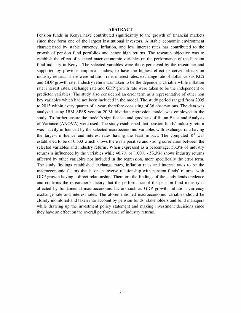
ABSTRACT

Pension funds in Kenya have contributed significantly to the growth of financial markets

since they form one of the largest institutional investors. A stable economic environment

characterized by stable currency, inflation, and low interest rates has contributed to the

growth of pension fund portfolios and hence high returns. The research objective was to

establish the effect of selected macroeconomic variables on the performance of the Pension

fund industry in Kenya. The selected variables were those perceived by the researcher and

supported by previous empirical studies, to have the highest effect perceived effects on

industry returns. These were inflation rate, interest rates, exchange rate of dollar versus KES

and GDP growth rate. Industry return was taken to be the dependent variable while inflation

rate, interest rates, exchange rate and GDP growth rate were taken to be the independent or

predictor variables. The study also considered an error term as a representative of other non

key variables which had not been included in the model. The study period ranged from 2005

to 2013 within every quarter of a year, therefore consisting of 36 observations. The data was

analyzed using IBM SPSS version 20.Multivariate regression model was employed in the

study. To further ensure the model’s significance and goodness of fit, an F test and Analysis

of Variance (ANOVA) were used. The study established that pension funds’ industry return

was heavily influenced by the selected macroeconomic variables with exchange rate having

the largest influence and interest rates having the least impact. The computed R2 was

established to be of 0.533 which shows there is a positive and strong correlation between the

selected variables and industry returns. When expressed as a percentage, 53.3% of industry

returns is influenced by the variables while 46.7% or (100% - 53.3%) shows industry returns

affected by other variables not included in the regression, more specifically the error term.

The study findings established exchange rates, inflation rates and interest rates to be the

macroeconomic factors that have an inverse relationship with pension funds’ returns, with

GDP growth having a direct relationship. Therefore the findings of the study lends credence

and confirms the researcher’s theory that the performance of the pension fund industry is

affected by fundamental macroeconomic factors such as GDP growth, inflation, currency

exchange rate and interest rates. The aforementioned macroeconomic variables should be

closely monitored and taken into account by pension funds’ stakeholders and fund managers

while drawing up the investment policy statement and making investment decisions since

they have an effect on the overall performance of industry returns.

1

CHAPTER ONE

INTRODUCTION

1.1 Background of the Study

Numerous studies have been conducted in developed capital markets with regard to

the relationship between asset prices and interest rates and results of most studies

suggest that stock and bond returns are predictable and that one may be used to

forecast the other. Whenever the interest rate on Treasury securities rises, investors

tend to switch out of stocks, causing stock prices to fall (Juli 2002). A precondition

for macroeconomic uncertainty to be related to volatility in financial markets is that

the new information released in the announcement moves asset prices. If financial

markets do not react to macroeconomic news, there is no reason to expect that

uncertainty about economic fundamentals is reflected in bond and stock market

volatility.

The stock exchange acts as the most important market for capital and a well

developed capital market is essential to promote economic development of any

country. Beber et al (2008), a number of researchers in various countries have found

significant relationships between macroeconomic variables and stock prices. These

studies concerned multi-factor models as well as single- factor models which

incorporate macroeconomic variables as explanatory factors of variation in equity

returns,

Roll and Ross (1980) posits that the factors derived by factor analysis should be

fundamental economic aggregates such as GNP or interest rates. Furthermore, they

acknowledged that the APT could not specify these economic factors. Finally they

suggested an investigation of economic factors that are proxy by derived factors in the

APT, Roll and Ross (1986) were the first to employ specific macroeconomic factors

as proxies for undefined variables in the APT. The three researchers attempted to

express the equity returns as a function of macroeconomic variables. Since economic

forces like interest rates, Treasury bill rates can influence expected dividends and the

discount rate, it was concluded that stock prices hence stock returns are systematically

affected by economic variables.

2

During the period 2011 to 2012, the Kenyan economy experienced high volatility in

some of the economy’s key macroeconomic variables that was characterized by very

high lending interest rates, high unexpected rates of inflation and a weakening of the

Kenya shilling against other currencies. This led to Central Bank of Kenya increasing

the base lending rates in a bid to cab inflation and stabilize the Kenya shilling. This

had an impact on the returns of various investments in the country since more funds

were being channeled towards consumption rather than investments. Nyamute (1998)

noted that the state of the economy influences the way stock prices move. When it’s a

period of depression or recession, investments (including investment in shares) are

depressed and therefore the demand for stocks will fall leading to the downward

change in their prices and the vice versa incase of economic boom.

In Kenya, Pension funds control relatively large amounts of capital and are among the

largest institutional investors. Their investments include stocks, bonds and deposits

among others. This study therefore aims to determine the effect of selected

macroeconomic variables on Pension fund returns, (Rono et al 2010).

1.1.1 Macroeconomic Variables

Brinson et al. (1991) defined macro economic variables as those that are pertinent to a

broad economy at the regional or national level and affect a large population rather

than a few selected individuals. The variables indentified as having major influence

include; inflation, gross domestic product (GDP), currency exchange rate, interest

rates, legal and regulatory environment and risk. Illo (2012) carried out a study to

establish the effect of macroeconomic factors affecting commercial banks financial

performance in Kenya. The author identified interest rates, GDP growth rate, currency

exchange rate, money supply and inflation as the main macroeconomic factors

affecting commercial banks financial performance.

The key macro-economic variables that influence the investment markets include

interest rates, inflation, economic growth, exchange rates, current account and fiscal

deficits. Although it has been debated whether economic news had a significant

impact on stock prices, Pearce, Roley (1985) and Wasserfallen (1989), it is now

widely understood that stock prices react in response to and that macroeconomic

3

variables have explanatory power over prices and returns. McQueen and Roley (1993)

show that the stock market response to macroeconomic news is dependent upon the

state of the economy, while Flannery and Protopapakis (2002) highlight that

macroeconomic factors influence both stock market volatility and returns.

The Kenyan financial markets have been greatly affected by market volatility in

recent years. The global financial crisis of 2008/2009 and the steep depreciation of the

Kenya shilling in 2011, all affected financial asset prices significantly. Pension

schemes as significant investors in financial assets have been significantly affected by

this volatility. There is no doubt that there has been significant market volatility as

evident from the NSE index, Treasury bill rate movement and offshore indices. This

has resulted mainly from aftershocks of the global financial crisis. The market

volatility has impacted on pension scheme performance very strongly, with good

period’s showing significant positive growth and bad periods of negative

performance. These swings are exacerbated by a significant negative correlation

between the NSE prices and interest rates on government securities which together

constitute 70% of pension scheme assets, (RBA policy briefs 2011/2012).

1.1.2 Portfolio Returns

According to Wiley et al. (2012), return is defined as the increase in the value of an

investment over a period of time, expressed as a percentage of the value of the

investment at the start of the period. Pension fund’s portfolio managers invest in

Listed Equities, Private Equity, government securities, commercial papers, corporate

bonds, call and term deposits, property and offshore. The Pension fund industry is

regulated by the Retirements Benefits Authority who set limits on the various asset

classes: RBA guidelines have limited pension fund portfolio managers to investing

mainly in government securities (90% r 100%) and NSE stock (70%) with only 30%

allowed for fixed deposits, 15% in offshore 30% in immovable property and real

estate and 10% in other assets. Therefore, pension fund investments are mainly

limited to bonds and equities listed at the Nairobi Securities Exchange, (RBA ACT

Rev 2010).

4

All the assets of a pension fund are usually marked to market. The closing prices are

often provided by the Nairobi Securities Exchange on a daily basis and are updated

into the fund managers and custodian systems at the end of every month. Therefore an

increase in market values of bonds and stocks reflects an increase in the portfolio

returns. These are captured as unrealized capital gains. Pension fund returns therefore

include, dividends on stocks, capital gains on stocks, coupons on government bonds,

capital gains from increments in valuation of bonds, interest on corporate bonds,

interest earned on call and fixed deposits, increase in the market value of property

owned by a scheme and increase in the market values and dividends on offshore

investments. Since RBA allows Pension fund to invest up to 70% in listed stocks and

up to 100% in treasury securities, it follows that pension fund portfolios mainly

consist of Stocks and treasury securities listed at the Nairobi Stock Exchange.

Therefore, this study will mainly focus on how the prices of the two asset classes are

affected by volatility of macroeconomic variables, (RBA ACT Rev 2010).

1.1.3 Effect of Macro Economic Variables on Portfolio Returns

Various theories such as the, modern portfolio theory and arbitrage pricing theory,

have established that macroeconomic variables specifically affecting portfolio returns

include; interest rate volatility, gross domestic product (GDP), currency exchange

rates, inflation, money supply and industrial production, asset prices are commonly

believed to react sensitively to economic news. Daily experience seems to support the

view that individual asset prices are influenced by a wide variety of unanticipated

events and that some events have a more pervasive effect on asset prices than do

others. Consistent with the ability of investors to diversify, modern financial theory

has focused on pervasive, or systematic, influences as the likely source of investment

risk, (Ross et al 1986).

Ross et al. (1986), points out those unanticipated changes in the riskless interest rate

will therefore influence pricing, and, through their influence on the time value of

future cash flows, they will influence returns. The discount rate also depends on the

risk premium; hence, unanticipated changes in the premium will influence return.

Changes in the expected rate of inflation would influence nominal expected cash

flows as well as the nominal rate of interest. To the extent that pricing is done in real

5

terms, unanticipated price-level changes will have a systematic effect, and to the

extent that relative prices change along with general inflation, there can also be a

change in asset valuation associated with changes in the average inflation rate.

According to Ross et al. (1986), there is no satisfactory theory would argue that the

relation between financial markets and the macro economy is entirely in one

direction. However, stock prices are usually considered as responding to external

forces, even though they may have a feedback on the other variables. It is apparent

that all economic variables are endogenous in some ultimate sense. By the

diversification argument that is implicit in capital market theory, only general

economic state variables will influence the pricing of large stock market aggregates.

Any systematic variables that affect the economy's pricing operator or that influence

dividends would also influence stock market returns.

Stock return volatility has been a concern in the financial sector around the world.

Stock markets in emerging market especially in African have gained prominence

since the market has developed a step further to risk diversification apart from the

primary role of providing an alternative source of capital for investment. High

volatility of stock return is attributable to high risk, since most investors are risk

averse; they tend to shy off from the market due to uncertainty in expected returns.

High market volatility increases unfavorable market risk premium. Therefore, it is

critical for policy makers to reduce the stock market volatility and ultimately enhance

economy stability in order to improve the effectiveness of the asset allocation

decisions (Poon and Tong, 2010).

Researchers have in the past concentrated on establishing the effects of foreign

exchange rate fluctuation on stock return volatility. Mixed results have been evident

with some results indicating that exchange rate fluctuation has an impact on stock

return volatility as some contradicting. Singh et al (2011) investigated the cause and

effect relationship of foreign exchange rate volatility with stock returns in Taiwan.

The findings of the study indicated a positive relationship and that foreign exchange

rate volatility has an impact of stock return volatility. Hsing (2011) too studied the

JSE using GARCH models and found a positive relationship between exchange rate

and stock return volatility.

6

1.1.4 Pension Funds in Kenya

A pension fund is a common asset pool meant to generate stable growth over the long

term, and provide pensions for employees when they reach the end of their working

years and commence retirement. Pension funds are established by employers to

facilitate and organize the investment of employees' retirement funds contributed by

both the employers and employees. In Kenya, pension funds are often referred to as

Retirement Benefits Schemes and are regulated by the Retirement Benefits Authority.

In most pension funds in Kenya, the employers contribute twice what the employees

contribute.

According to the Retirement Benefits Act, retirement benefits scheme” means any

scheme or arrangement (other than a contract for life assurance) whether established

by a written law for the time being in force or by any other instrument, under which

persons are entitled to benefits in the form of payments, determined by age, length of

service, amount of earnings or otherwise and payable primarily upon retirement, or

upon death, termination of service, or Retirement Benefits Act (Cap. 197 ) upon the

occurrence of such other event as may be specified in such written law or other

instrument.

Pension funds in Kenya have contributed significantly to the growth of financial

markets since they form one of the largest institutional investors. A stable economic

environment characterized by stable currency, inflation, and low interest rates has

contributed to the growth of pension fund portfolios and hence high returns. However,

when interest rates shot up in 2011/2012, the stock and bond prices of existing bonds

declined sharply, and since the assets have to be marked to market, this adversely

affected the portfolio of most schemes such that majority of them reported negative

returns for that year RBA policy briefs (2012). Due to the increase in inflation,

companies overhead cost increased causing their net returns to decrease. This also

resulted to a decline in the dividends by most companies listed at the Nairobi

Securities Exchange. As a result, members retiring and hence leaving the schemes

during the period had to consider either deferring their benefits until the market

recovered or cashing in negative returns. This put fund managers on the spot with the

beneficiaries of the pension funds since it contradicted the purpose of a pension

7

scheme which is to save and investors expect their savings to gain interest not erode

their savings.

1.2 Research Problem

According to CAPM, macro-economic variables form the systematic risk component

in a portfolio and as such the effects are not diversifiable. According to Kung’u

(2013), a positive relationship, depicted by increased portfolio returns, is expected

between the rate of GDP growth, stable inflation, low interest rates and appreciation

of the Kenya shilling versus a foreign currency. However a negative relationship,

depicted by a drop in portfolio returns, is expected between unexpected inflation

increased lending interest rates, decreased GDP growth and depreciation of the Kenya

shilling. There are other variables which have an impact on portfolio returns, such as

size of the fund, asset allocation by fund managers, asset selection and market timing.

In Kenya various institutions invest in the financial markets, these include insurance

companies, unit trusts, commercial banks and Pension schemes. Portfolio managers

prefer to diversify their investments into the various classes mainly shares, bonds and

bank deposits. According to Economic Survey (2010), the average interest rate on 91-

day treasury bills fell to 6.82 % in December 2009 from 8.59% in December 2008.

Inflation eased from 16.2% in 2008 to 9.2% in 2009 (KNBS, 2010). The average

annual inflation was 4.1 percent in 2010 down from a high of 10.5 percent recorded in

2009 (KNBS, 2011). During this period, the stock market experienced recovery

therefore resulting to positive returns on investments. However, in the period

2011/2012 the Kenyan Economy experienced high volatility in its key economic

variables which was characterized by high unexpected inflation, depreciation of the

local currency and high interest rates. This impacted greatly on the financial markets,

the stock market prices and bond values declined sharply, resulting into low and in

some cases, negative returns on investments.

A lot of research has been carried recently on the effect of macroeconomic variables

on stock prices of companies listed at Nairobi Securities Exchange. Maina (2011)

found that share prices are affected by macroeconomic variables, Kungu (2013) found

that financial performance of Private Equity firms is affected by fundamental

macroeconomic factors such as GDP, inflation, currency exchange rate, interest

8

lending rates and market risk, while Olweny (2011) concluded that, foreign exchange

rate, Interest rate and Inflation rate, affect stock return.

However, there exists a research gap since these studies focus on how prices of stocks

are affected by volatility of macroeconomic variables and therefore fail to consider

that institutional investors diversify their portfolios into different asset classes. There

is also a research gap since some of the studies done indicate that the effect of

macroeconomic variables on returns is present but not significant. This study will

therefore seek to focus how the returns of a portfolio consisting of various asset

classes namely, listed stocks and corporate bonds, government securities and bank

deposits is affected by volatility in key macroeconomic variables and conclusively

answer the question; what is the effect of volatility of macroeconomic variables on the

returns of pension funds’ returns in Kenya?

1.3 Objective of the Study

To establish the relationship between macro-economic variables and portfolio returns

of pension funds in Kenya.

1.4 Value of the Study

The findings of the study will help the portfolio managers to better predict the effects

of the macroeconomic variables on their portfolios in good time to be able to hedge or

reduce the negative impacts in bad seasons in as well as maximize returns in good

seasons.

The findings of the study will also be useful to the RBA, by providing information

that will further assist in establishing policies that will ensure that pensioners’ returns

are maximized and objectives of pension schemes are met.

The findings can also be used by to Central Bank of Kenya in managing monetary

policy while at the same time ensuring investments and economic growth is not

affected.

The findings will guide trustees of pension funds in better understanding their

investments and in making Investment decisions on assets that respond to the macro-

economic variables environment while maintaining the limits set by RBA and the

Investment Policy Statement.

9

The empirical findings of this proposed research will also contribute to the body of

knowledge on financial markets and pension funds in Kenya.

10

CHAPTER TWO

LITERATURE REVIEW

2.1 Introduction

This chapter will review the theories guiding the study, followed by a review of the

previous theoretical and empirical literature on the role of macroeconomic variables

in determining portfolio returns. The chapter will be completed by a section of

conclusions from the literature review indicating the gaps that the literature is

addressing.

2.2 Theoretical Review

This section discusses the theories such as portfolio theory, CAPM and APT that

explain portfolio returns with relation to systematic and unsystematic risk. The

theories identify systematic risk as that which cannot be diversified away such as

variability on macroeconomic variables and political upheavals. The EMH explains

that in an efficient market; where all information is available to all parties at the same

time, it is impossible to make abnormal returns.

2.2.1 Portfolio Theory

The basic portfolio model was developed by Markowitz (1952) and one basic

assumption of this theory is that as an investor you want to maximize the returns from

your investments for a given level of risk. According to Markowitz, the full spectrum

of investments must be considered because the returns from all these investments

interact, and this relationship between the returns for assets in the portfolio is

important.

Markowitz (1952) contends that investors are basically risk averse; meaning that,

given a choice between two assets with equal rates of return, they will select the asset

with the lower level of risk. Therefore there is generally a positive relationship

between the rates of return on various assets and their measures of risk. Markowitz

derived the expected rate of return for a portfolio of assets and an expected risk

measure. Markowitz also showed that the variance of the rate of return was a

meaningful measure of portfolio risk under a reasonable set of assumptions, and he

derived the formula for computing the variance of a portfolio. This portfolio variance

11

formula indicated the importance of diversifying your investments to reduce the total

risk of a portfolio and also showed how to effectively diversify.

According to Markowitz (1952), a single asset or portfolio of assets is considered to

be efficient if no other asset or portfolio of assets offers higher expected return with

the same or lower risk, or lower risk with the same or higher expected return. One of

the best-known measures of risk is the variance, or standard deviation of expected

returns. It is a statistical measure of the dispersion of returns around the expected

value whereby larger variance or standard deviation indicates greater dispersion. The

idea is that the more disperse the expected returns, the greater the uncertainty of

future returns. The expected rate of return for a portfolio of investments is simply the

weighted average of the expected rates of return for the individual investments in the

portfolio. The weights are the proportion of total value for the investment. The

variance, or standard deviation, is a measure of the variation of possible rates of

return, from the expected rate of return.

2.2.2 Capital Asset Pricing Model

The Capital Asset Pricing Model (CAPM) was developed in the 1960s by Sharpe

(1964), Treynor (1962), Lintner (1965) and Mossin(1966) .It is an extension of the

portfolio theory and develops a model for pricing all risky assets. It allows investors

to determine the required rate of return for any risky asset. The major factor that

allowed portfolio theory to develop into capital market theory is the concept of a risk-

free asset. Several authors considered the implications of assuming the existence of a

risk-free asset, that is, an asset with zero variance. Such an asset would have zero

correlation with all other risky assets and would provide the risk-free rate of return

(RFR).A risky asset is one from which future returns are uncertain, and this

uncertainty is measured by the variance, or standard deviation, of expected returns.

According to Sharpe (1964), a portfolio that includes all risky assets is referred to as

the market portfolio. Since the market portfolio contains all risky assets, it is a

completely diversified portfolio meaning that all the risk unique to individual assets in

the portfolio is diversified away. Specifically, the unique risk of any single asset is

offset by the unique variability of all the other assets in the portfolio. This unique

12

(diversifiable) risk is also referred to as unsystematic risk. This implies that only

systematic risk, which is defined as the variability in all risky assets caused by

macroeconomic variables, remains in the market portfolio. This systematic risk,

measured by the standard deviation of returns of the market portfolio, can change over

time if and when there are changes in the macroeconomic variables that affect the

valuation of all risky assets.

Examples of such macroeconomic variables would be variability of growth in the

money supply, interest rate volatility, and variability in such factors as industrial

production, corporate earnings, and corporate cash flow. The standard deviation of

your portfolio will eventually reach the level of the market portfolio, where you will

have diversified away all unsystematic risk, but you still have market or systematic

risk. You cannot eliminate the variability and uncertainty of macroeconomic factors

that affect all risky assets,

2.2.3 Arbitrage Pricing Theory

The Arbitrage Pricing Theory (APT) was originally developed by Ross (1976).It is a

one-period model in which every investor believes that the stochastic properties of

returns of capital assets are consistent with a factor structure. Ross argues that if

equilibrium prices offer no arbitrage opportunities over static portfolios of the assets,

then the expected returns on the assets are approximately linearly related to the factor

loadings. The factor loadings, or betas, are proportional to the returns’ covariances

with the factors.

The APT contends that there are many such factors that affect returns, in contrast to

the CAPM, where the only relevant risk to measure is the covariance of the asset with

the market portfolio that is, the asset’s beta. These factors include, inflation, growth in

GNP, major political upheavals changes in interest rates among others. However, in

application of the theory, the factors are not identified (Reilly and Brown, 2011).

The model-derived rate of return will then be used to price the asset correctly, the

asset price should equal the expected end of period price discounted at the rate

implied by model. If the price diverges, arbitrage should bring it back into line. The

13

theory is based on the idea that, in competitive financial markets arbitrage will assure

equilibrium pricing according to risk and return. Similar to the CAPM, the unique

effects are independent and will be diversified away in a large portfolio APT assumes

that, in equilibrium, the return on a zero-investment, zero-systematic-risk portfolio is

zero when the unique effects are diversified away (Reilly and Brown, 2011).

2.2.4 Multi-Factor Models

The multi factor models such as the Henrikson in 1984 use the concept of arbitrage

pricing model by introducing more factors in the model to introduce the excess return

of an equally weighted portfolio of the funds. Bello and Janjigian (1997) proposed an

extended Treynor and Mazuy’s measure to cover assets that are not in the main index

used to encompass the case of funds that includes bonds. For more general hybrid

funds, Comer (2006) suggested a multi-factor timing measure to consider systematic

risks of the funds to the market, to small stocks, to growing stocks, to long maturity

bonds, to short maturity bonds, to high quality bonds and to low quality bonds.

Henriksson (1984) tried to solve problems that might happen due to both the omission

of relevant factors and issues concerning the choice of the benchmark portfolio in the

Henriksson and Merton model (1981).

Henriksson and Merton (1981) extended measure of market timing includes two more

factors and a second dummy variable to introduce the excess return of an equally

weighted portfolio of the funds. Finally, Chan et al. (2002) proposed a Henriksson and

Merton timing measure in a three factor context, which is computed with the same

three factor model of Fama and French. Ferson and Schadt (1996) proposed a

conditional model that produces conditional betas. By extension, they proposed to

consider a conditional Treynor and Mazuy’s coefficient and a conditional Henriksson

and Merton’s coefficient.

2.2.5 Efficient Market Hypothesis

Fama (1970) presented the efficient market theory in terms of a fair game model,

contending that investors can be confident that a current market price fully reflects all

available information about a security and the expected return based upon this price is

14

consistent with its risk. There are three forms of market efficiency; weak form, semi

strong form and strong form which are discussed below:

The weak-form EMH assumes that current stock prices fully reflect all security

market information, including the historical sequence of prices, rates of return, trading

volume data, and other market-generated information, such as odd-lot transactions,

block trades, and transactions by exchange specialists. Because it assumes that current

market prices already reflect all past returns and any other security market

information, this hypothesis implies that past rates of return and other historical

market data should have no relationship with future rates of return(that is, rates of

return should be independent). Therefore, this hypothesis contends that you should

gain little from using any trading rule that decides whether to buy or sell a security

based on past rates of return or any other past market data.

The semi-strong form asserts that security prices adjust rapidly to the release of all

public information; that is, current security prices fully reflect all public information.

Public information also includes all nonmarket information, such as earnings and

dividend announcements, price-to-earnings (P/E) ratios, dividend-yield (D/P) ratios,

price book value (P/BV) ratios, stock splits, news about the economy, and political

news. This hypothesis implies that investors who base their decisions on any

important new information after it is public should not derive above-average risk-

adjusted profits from their transactions, considering the cost of trading because the

security price already reflects all such new public information.

The strong-form EMH contends that stock prices fully reflect all information from

public and private sources. This means that no group of investors has monopolistic

access to information relevant to the formation of prices. Therefore, this hypothesis

contends that no group of investors should be able to consistently derive above-

average risk-adjusted rates of return. The strong form EMH encompasses both the

weak-form and the semi strong-form EMH. Further, the strong form EMH extends the

assumption of efficient markets, in which prices adjust rapidly to the release of new

public information, to assume perfect markets, in which all information is cost free

and available to everyone at the same time.

15

2.3 Determinants of Portfolio Returns

This section discusses the factors that determine variations in portfolio returns and the

different strategies used by portfolio managers in trying to maximize investors’

returns.

2.3.1 Macroeconomic Variables

It is commonly believed that asset prices react sensitively to economic news.

Macroeconomic variables (GDP, currency exchange rates, inflation, money supply

and industrial production), have explanatory power over prices and returns. Recession

and unexpected increased in inflation reduces investor confidence in the market leads

to a fall prices since the profitability of corporates. News of a recovery in the

economy enhances investor confidence which in turn leads to a rise in asset prices.

Errunza and Hogan (1998), highlighted that macroeconomic factors can influence

both stock market volatility and returns.

2.3.2 Investment Policy

This is also known as strategic asset allocation. It deals with how investors divide

their portfolio among three major asset categories: cash, bonds and stocks. The asset-

allocation decision, otherwise known as investment policy, is arguably the most

important determinant of a portfolio's long-term return. A study by landmark Brinson,

Hood and Beebower, "Determinants of Portfolio Performance" (1986, 1991) argues

that investment policy accounts for 94% of the variation in returns in a portfolio,

leaving market timing and stock selection to account for only 6%. In their sample of

pension plans, active investment decisions by plan sponsors and managers, both in

terms of selection and timing, did little to improve performance over the 10-year

period from December 1977 to December 1987.

2.3.3 Security Selection

This refers to the choice of specific securities within an asset class. Based on risk

considerations, the investor establishes the asset allocation strategy. Trading

strategies, rules and concepts based on fundamental and technical analysis have been

devised by both academics and practitioners in assisting the investors in their decision

making process. Innovative investors opt to employ information technology to

16

improve the efficiency in the process. This is done through transforming trading

strategies into computer known languages so as to exploit the logical processing

power of the computer. This greatly reduces the time and effort in short-listing the list

of attractive stocks. Hoernemann et al (2005), challenges the prevalent notion that

more than 90% of the variability of returns is determined by strategic asset allocation.

They then present an alternative study, which uses a slightly different framework and

covers a longer time horizon than the earlier work, includes alternative assets, and

utilizes synthetic portfolios. Using identical calculations, they find that on average

strategic asset allocation explained 77.5% of the variability of portfolio returns, while

security selection accounted for 10.3%, and tactical asset allocation explained 5.6%.

Though the authors thus agree that strategic asset allocation is a major determinant of

investment performance, they argue that the investment process should not be limited

to strategic asset allocation, as managers can potentially add value through tactical

asset allocation and security selection. Although the contributions of security

selection and tactical asset allocation may seem small, the power of compounding

returns makes them significant to individual investors.

2.3.4 Market Timing

This is the act of attempting to predict the future direction of the market, typically

through the use of technical indicators or economic data. According to Jagannathan et

al. (1985), market timing is a strategy in which the investor tries to identify the best

times to be in the market and when to get out. Relying heavily on forecasts and

market analysis, market timing is often utilized by brokers, financial analysts, and

mutual fund portfolio managers to attempt to reap the greatest rewards for their

clients. Managers may adjust the interest rate sensitivity such as duration of the

portfolio to time changes in interest rates. They may vary the allocation to asset

classes differing in credit risk or liquidity, and tune the portfolio’s exposure to other

economic factors.

17

2.4 Empirical Review

This section reviews previous research done on the effect of macroeconomic variables

on asset prices and returns, both locally and internationally.

2.4.1 International Evidence

Feldestein (1983) carried out a study to investigate the relationship between inflation

and the stock market in the US and found that when the steady-state rate of inflation is

higher, share prices increase at a faster rate. More specifically, when the inflation rate

is steady, share prices rise in proportion to the price level to maintain a constant ratio

of share prices to real earnings. In contrast, an increase in the expected future rate of

inflation causes a concurrent fall in the ratio of share prices to current earnings.

Although share prices then rise from this lower level at the higher rate of inflation, the

ratio of share prices to real earnings is permanently lower. This permanent reduction

in the price-earnings ratio occurs because, under prevailing tax rules, inflation raises

the effective tax rate on corporate source income. Inflation rate is defined as the rate,

at which prices generally increase. In order to understand the structural relation

between inflation and share prices, it is crucial to distinguish between the effect of a

high constant rate of inflation and the effect of an increase in the rate of inflation

expected for the future.

Jorion (1990) sought to investigate the exchange rate exposure on U.S multinationals.

He found that those exchange rates were four times as volatile as interest rates and ten

times as volatile as inflation rates. The rapid expansion in international trade and the

adoption of floating exchange rates by countries in the developed and developing

world was a harbinger of a new era of increased foreign exchange volatility For the

Investor, changes in exchange rates poses a foreign exchange risk. High fluctuations

in exchange rates can lead to big losses in an investor’s portfolio of investments due

to uncertainty of return on investments. This is due to the fact that movements in

foreign exchange rates affect the prices of goods on the international markets and this

in turn affects the profit margin of exporting and importing companies.

Ritter (2004) studied the relationship between economic growth and equity returns in,

using data for the period 1900 to 2002. He found that for 16 countries representing

perhaps 90% f world market capitalization in 1900, there was a negative correlation

18

between per capita income growth and real equity returns. In the short run there is

ample evidence that unexpected changes in economic growth affect stock prices.

Stock prices decline when the probability of an economic recession increases, since

recession affects corporate profitability and stock prices increase when the probability

of economic recovery increases. The effects should however be transitory and should

not have a significant effect on the present value of dividends for a given firm.

Though economic growth does result in a higher standard of living for consumers, it

does not necessarily translate into higher present value of dividends per share for the

owners of the existing capital stock. As such he concluded that whether future

economic growth is high or low in given country has little to do with future equity

returns in that country.

Humpe and Macmillian (2007) carried out a study to investigate the relationship that

exists between a number of macroeconomic variables and stock prices in the US and

Japan within the framework of a standard discount model. They applied co integration

analysis using Johansen (1991) procedure in order to model the long term relationship

between industrial productions. The macroeconomic variables used were consumer

price index, long term interest rates and stock prices in the US and Japan. Using the

US data they found evidence of a single co integration vector between stock prices,

interest rates, industrial production, inflation and long term interest rates. In their

findings, stock prices were positively related to industrial production, inflation and

long term interest rates. However, they found an insignificant (although positive)

relationship between US stock prices and interest rates. For Japanese data they found

two co integrating vectors. The first one provided that stock prices are positively

related to industrial production but negatively related to interest rates. The second one

found out that industrial production was negatively related to interest rate and the rate

of inflation. This is because a rise in the interest rate reduces the present value of

future dividend’s income, which should depress stock prices. Conversely, low interest

rates result in a lower opportunity cost of borrowing. Lower interest rates stimulate

investments and economic activities, which would cause prices to rise.

Gazi and Mahmudul (2009) sought to find evidence supporting the existence of share

market efficiency based on the monthly data from January 1988 to March 2003 and

also show empirical relationship between stock index and interest rate for fifteen

19

developed and developing countries. To investigate the reasons of market

inefficiency, relationship between share price and interest rate and changes of share

price and changes in interest rate were determined through both time series and panel

regressions. For all of the countries it is found that interest rate has significant

negative relationship with share price and for six countries, it is found that changes of

interest rate has significant negative relationship with changes of share price.

2.4.2 Local Evidence

Olweny and Omondi (2011) sought to investigate the effect of Macro-economic

factors on the stock return volatility on the Nairobi Securities Exchange, Kenya. The

study focused on the effect of foreign exchange rate, interest rate and inflation rate

fluctuation on stock return volatility at the Nairobi Securities Exchange. It used

monthly time series data for a ten years period between January 2001 and December

2010. Empirical analysis employed was Exponential Generalized Autoregressive

Conditional Heteroscedasticity (EGARCH) and Threshold Generalized Conditional

Heteroscedasticity (TGARCH). The main findings of the research study are as

follows: the stock returns are symmetric but leptokurtic and not normally distributed.

The results showed evidence that Foreign exchange rate, Interest rate and Inflation

rate, affect stock return volatility. On foreign exchange rate, magnitude of volatility is

relatively low at 0.209138 and significant since the probability is almost zero, 0.3191.

This implies that the impact of foreign exchange on stock returns is relatively low

though significant. Volatility persistence was found low at -0.251925 and significant.

This implies the effect of shocks takes a short time to die out following a crisis

irrespective of what happens to the market. There was evidence of leverage effect

0.6720. This means that volatility rise more following a large price fall than following

a price rise of the same magnitude.

Kasuvu (2012) examined the effects inflation on investment in treasury securities by

Commercial banks in Kenya. The study used a descriptive survey and covered the

period from 2001 to 2011. The findings show that that there is no significant

relationship between inflation rate and investment in treasury securities by

commercial banks in Kenya. Further it found that there is no significant relationship

between level of investment in treasury securities by commercial banks and lending

20

rates offered by Kenyan banks. However the study shows that there is significant

relationship between level of investment in treasury securities and maturity periods of

treasury bonds.

Sifunjo and Mwasaru (2012) examined the causal relationship between foreign

exchange rates and stock prices in Kenya from November 1993 to May 1999. The

data set consisted of monthly observations of the NSE stock price index and the

nominal Kenya shillings per US dollar exchange rates. The objective was to establish

the causal linkages between leading prices in the foreign exchange market and the

Nairobi Securities Exchange (NSE). The empirical results show that foreign exchange

rates and stock prices are non stationary both in first differences and level forms, and

the two variables are integrated of order one, in Kenya. Secondly, the study tested for

co integration between exchange rates and stock prices. The results show that the two

variables are co integrated. Thirdly, the study used error-correction models instead of

the classical Granger-causality tests since the two variables are co integrated. The

empirical results indicated that exchange rates Granger-causes stock prices in Kenya.

There is unidirectional causality from exchange rates to stock prices.

From this study, the direction of Granger-causality from exchange rates to stock

prices has a numbers of implications for individual investors, corporate investors,

financial regulators and market intermediaries. Sharp fluctuations in the stock prices

arising from fluctuations in foreign exchange rates can cause panic among portfolio

managers. This will induce them to liquidate portions of their portfolios to hedge

against currency losses. The net impact will be a slump in the NSE index, an indicator

of poor trading condition on the stock market. High volatility in the stock market

makes it difficult for investors in the foreign exchange market and stock market to

protect their investment against an adverse turn in market developments.

Chirchir (2013) carried out a study to examine how changes in interest rates

(represented by the weighted average lending rate by commercial banks in Kenya)

and stock prices ( proxied by the NSE 20 share index) are related to each other for

Kenya over the period October 2002 to September 2012. The research used Toda and

Yamamoto (1995) method to determine the relationship between stock prices and

21

interest rates. The results indicated that there is no significant causal relationship

between interest rate and share price. However he also observed that when interest

rates increase the share prices decline which attests to the expected relationship as

proposed by Fama.

Mmasi (2013) sought to assess the causality relationship between inflation and

interest rate in Kenya. The study used a correlational design using

secondarydatafrom1961 to 2011 on interest rate, inflation rate, money supply, and

GDP growth rates. Analysis was performed using descriptive analysis, Granger-

causality tests, correlation analysis, and regression analysis. On the causal relationship

between interest rate and inflation rate, the study found unidirectional relationship

which ran from inflation to interest rate. With the direction of relationship examined,

a further analysis was run to examine whether inflation rate significantly influenced

interest rate. The study revealed that inflation rate did not have a significant impact on

interest rate. The results further showed that GDP growth has a negative and

significant impact on interest rates in Kenya while money supply had a positive and

significant impact on interest rate. The study concludes that there is a unidirectional

relationship that runs from inflation to interest rates. The study further concludes that

inflation does not have significant effect interest rates but GDP growth and money

supply have a significant impact on interest rates in Kenya.

Ombaka (2013) carried out a study to establish the effect of inflation and money supply on

the returns of firms listed at the Nairobi Securities Exchange. The study adopted correlation

study design and monthly empirical time series data to analyze and describe the effect of

inflation and money supply on the returns of firms listed at Nairobi Securities Exchange.

Secondary data on consumer price index, money supply and Nairobi Securities Exchange all

share index (NASI) was used to describe the relationship between the variables. The study

found out that Stock Market Returns seems to have decreased as a result of increase in

inflation meaning that the two variables have an inverse relationship. The study found out that

a unit increase in inflation leads to 2.741 decreases in Stock Market Returns. On the other

hand, it was found that Money Supply has a positive relationship with Stock Market Returns.

The study found out that a unit increase in Money Supply leads to 0.054 increases in Stock

Market Returns. The findings of this study show that both Inflation and Money Supply

explains only 36.1% of the change in Stock Market Returns. This implies that the changes in

22

Stock Market Returns are largely affected by other factors other than the two. The study

found out that Stock Market Returns seems to have decreased as a result of increase in

inflation meaning that the two variables have an inverse relationship. The study found

out that a unit increase in inflation leads to 2.741 decreases in Stock Market Returns.

He also found that Money Supply has a positive relationship with Stock Market

Returns. The study found out that a unit increase in Money Supply leads to 0.054

increases in Stock Market Returns. The findings of his study however show that both

Inflation and Money Supply explains only 36.1% of the change in Stock Market

Returns.

2.5 Summary of the Literature Review

From the studies conducted earlier, it is evident that macroeconomic variables

selected to examine the determinants of stock prices differ slightly across studies. A

significant part of the existing literature has established the relations between

macroeconomic variables and stock prices indicating a unidirectional causality

running from the macro environment to the financial markets. Some of the studies

done conclude that there is indeed a relationship between macro-economic variables

and asset prices. However, there exists a research gap since the researches differ on

the level significance of these effects on portfolio returns. Kasuvu (2012) concludes

that there is no significant relationship between inflation rate and investment in

treasury securities, while Mmasi (2013) concludes that the direction of the

relationship between inflation and interest rate in Kenya is unidirectional indicating

therefore that an increase in inflation results to increased interest rates which in turn

increase the coupon rate for treasury bond issued by the government. Chirchir (2013)

concludes that there is no significant causal relationship between interest rate and

share price while Fama 1981explains that in theory, the interest rates and the stock

prices have a negative correlation since a rise in the interest rate reduces the present

value of future dividend’s income, which should depress stock prices. Jorion (1990)

points out that for the Investor, changes in exchange rates poses a foreign exchange

risk and as such high fluctuations in exchange rates, can lead to big losses in an

investor’s portfolio of investments due to uncertainty of return on investments.

However, according to the research by Olweny and Omondi (2011) the impact of

foreign exchange on stock returns is relatively low though significant.

23

The study therefore aims to give conclusive results on the significance of the

volatility of selected macroeconomic variables. It is also evident from the studies

done that the focus has mainly been on the relationship between macroeconomic

variables and the stocks listed at the Nairobi Securities Exchange. There are however

various investment classes that institutional investors have at their disposal. Stocks are

considered to be risky assets and as such institutional investors like pension funds,

insurance companies, mutual funds, prefer to diversify their portfolio with the aim of

hedging against adverse effects in the stock market. This research therefore will look

at a portfolio as containing not only of listed stocks, but also other assets such as

treasury bonds, corporate bonds, deposits, offshore securities and property. The aim is

to determine the effect of macroeconomic variables on the returns of a portfolio that is

diversified into the various asset classes, by examining the effect of macroeconomic

variables on the quarterly industry returns of the pension funds in Kenya.

24

CHAPTER THREE

RESEARCH METHODOLOGY

3.1 Introduction

This chapter outlines the methodological techniques that were used in the study. The

section describes the research design, data collection, data analysis and lastly the

model that was used in the study.

3.2 Research Design

A research design is a plan, structure and strategy of investigation conceived with the

aim of obtaining answers to a research question or problem. This study used

descriptive case study to determine the relationship between macroeconomic variables

(GDP growth, inflation, interest rates and exchange rates) and average pension

industry returns. To define the descriptive type of research, Creswell (1994) stated

that the descriptive method of research is to gather information about the present

existing condition. Descriptive research reports the percentage summary on a single

variable. The aim of descriptive research is to verify formulated hypotheses or

research questions that refer to the present situation in order to explain it. The results

verified formulated hypothesis from existing theories and those formed from

empirical studies carried out on the area.

3.3 Data Collection

Data for this study was from secondary sources. The data was obtained from Kenya

National Bureau of Statistics, Central Bank of Kenya, Nairobi Securities Exchange

and Government of Kenya publications, Pension Scheme administrators, Alexander

Forbes actuaries, fund managers and custodians. Industry returns were measured by

the time weighted return, Interest rates were measured using the 91 day Treasury bill

rate, exchange rate was measured in Kenya shillings against the US dollar, and annual

inflation rate and GDP growth rate were also used. The study used quarterly data for

the period 2005 to 2013.

25

3.4 Data Analysis

The study was aimed to establish the relationship between industry returns and

macroeconomic variables. Multiple regression analysis was used based on arbitrage

pricing theory.

3.4.1 Analytical Model

The regression equation tested was as follows;

Rt = βo + β1 INF + β2 INT + β3EXR+ β4GDP+e Where;

Rt= quarterly Industry Returns (from Alexander Forbes quarterly afcass reports)

INF = quarterly annual Inflation rate

INT = quarterly annual Interest rate

EXR = quarterly annual Exchange rate

GDP = quarterly GDP growth rate

β0 = Constant term

βi = coefficient of variable i which measures the change in industry returns as a result

of a unit change in the selected macroeconomic variables.

e = error term which measures variations in the dependent variable not explained by

the model which means there are other factors that influence the industry returns.

The package used was IBM Statistical Package for the Social Scientist (SPSS) and

data analysis was done using summary statistics, correlation analysis and regression

analysis. These techniques will be were used to explain the relationship between the

dependent variable (industry returns) and independent variables (inflation rate,

interest rate, exchange rate, GDP).

3.4.2 Test of significance

The study tested the level of statistical significance of the findings of at5% using the

Analysis of variance technique (ANOVA). A 5% level of significance is another way

of saying that 95% of the time that a sample is taken from the population, the study

will be likely to generate the same results. The ANOVA solves the difficulty that

arises with either z-test or t-test when examining the significance of the difference

amongst more than two samples at the same time. If the results of the test fall within

the 5% level of significance, it means that the sample selected is a true representation

of the population.

26

CHAPTER FOUR

DATA ANALYSIS, RESULTS AND DISCUSSION

4.1 Introduction

This chapter presents the results, finding and discussion with reference to and based on

the research topic and study objectives. The results are shown in summary tables and

analysis charts. The data used in this study was primarily obtained from KNBS, afcass

actuary reports, CBK and fund managers reports. Multivariate linear regression has been

employed in this study where a number of selected independent variables such as

inflation rate, interest rate, exchange rate and GDP growth rate are regressed against a

restricted and identified dependent variable which is industry returns of pension funds. A

goodness of fit statistic, confidence interval and correlation analysis has been employed

to further explain the relationship between the independent macroeconomic variables and

industry returns.

4.2 Descriptive Statistics

This section describes the main features of data collection quantitatively for simpler

interpretation of the data.

4.2.1 Descriptive Statistics of the Variables

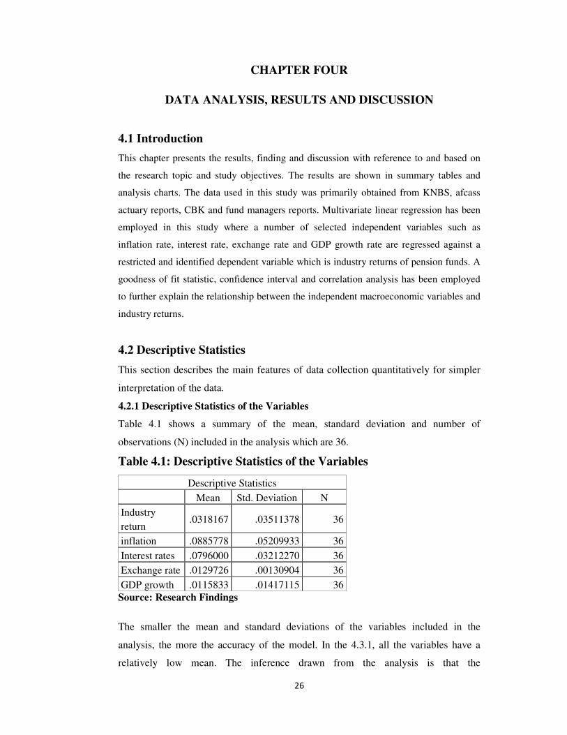
Table 4.1 shows a summary of the mean, standard deviation and number of

observations (N) included in the analysis which are 36.

Table 4.1: Descriptive Statistics of the Variables

Descriptive Statistics

Mean Std. Deviation N

Industry

return .0318167 .03511378 36

inflation .0885778 .05209933 36

Interest rates .0796000 .03212270 36

Exchange rate .0129726 .00130904 36

GDP growth .0115833 .01417115 36

Source: Research Findings

The smaller the mean and standard deviations of the variables included in the

analysis, the more the accuracy of the model. In the 4.3.1, all the variables have a

relatively low mean. The inference drawn from the analysis is that the

27

macroeconomic variables have a significant impact on the industry returns of pension

funds.

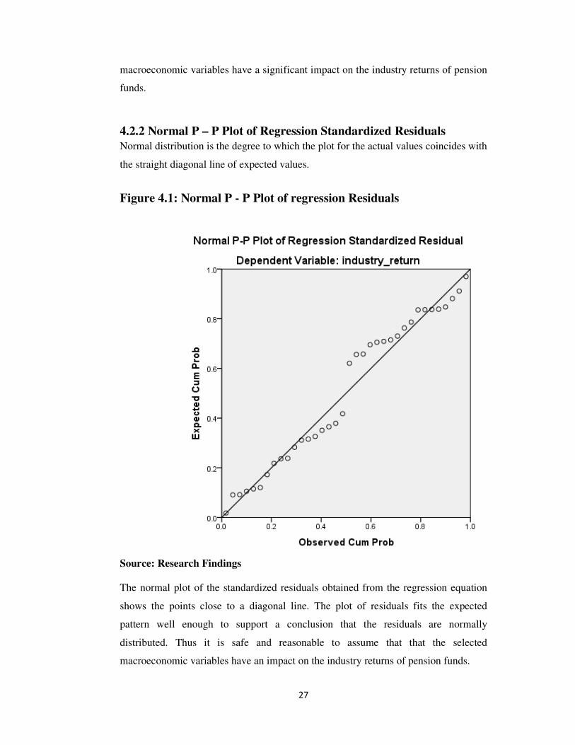
4.2.2 Normal P – P Plot of Regression Standardized Residuals

Normal distribution is the degree to which the plot for the actual values coincides with

the straight diagonal line of expected values.

Figure 4.1: Normal P - P Plot of regression Residuals

Source: Research Findings

The normal plot of the standardized residuals obtained from the regression equation

shows the points close to a diagonal line. The plot of residuals fits the expected

pattern well enough to support a conclusion that the residuals are normally

distributed. Thus it is safe and reasonable to assume that that the selected

macroeconomic variables have an impact on the industry returns of pension funds.

28

4.3 Inferential Statistics

This section of data analysis extends beyond the immediate data to properties of the

data that will be used to make judgments, by determining the relationship between the

independent and dependent variables, their correlation, the significance of their

relationship and the goodness of fit of the model.

4.3.1 Correlation Analysis

The correlation coefficient is a measure of linear association between two variables. It

measures of the strength of the association between the two variables. This data

analysis used the Pearson's correlation coefficient between two variables which is

defined as the covariance of the two variables divided by the product of their standard

deviations.

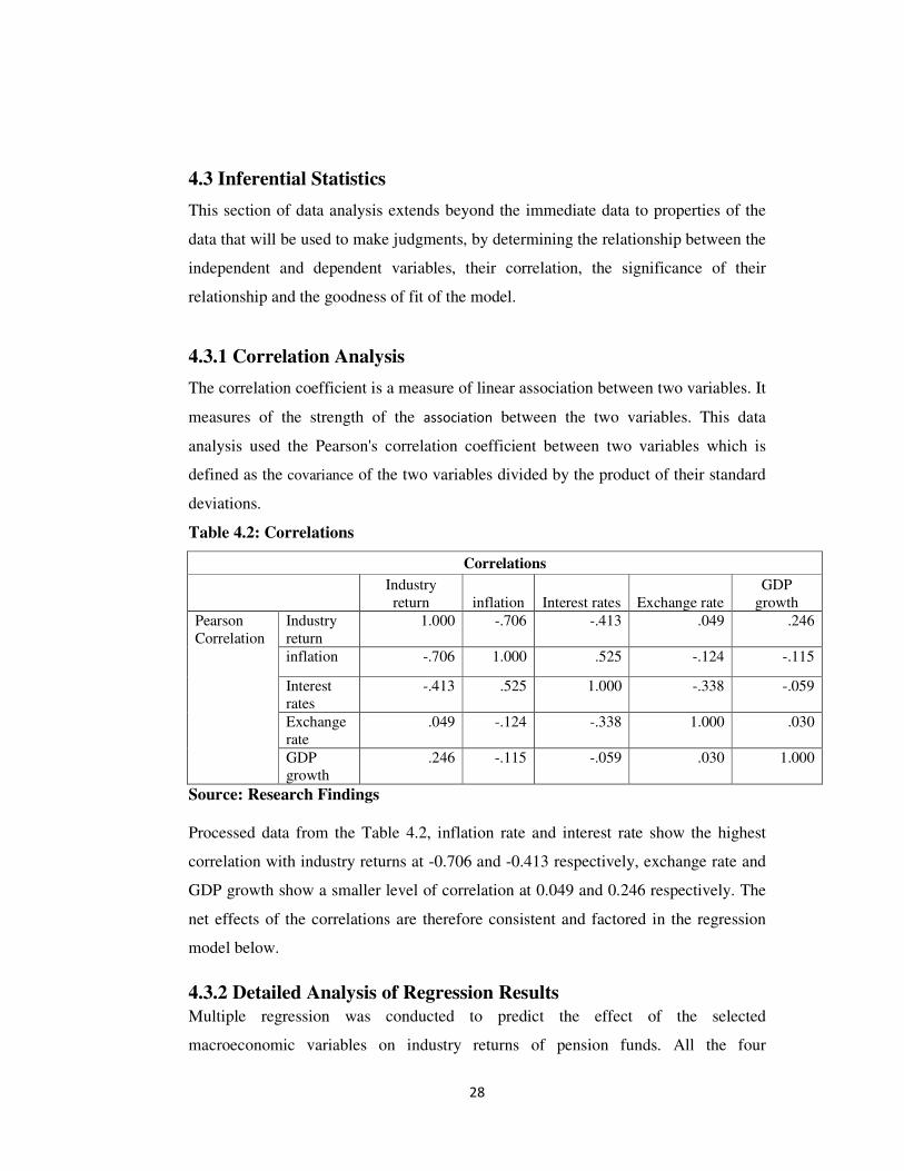
Table 4.2: Correlations

Correlations

Industry

return inflation Interest rates Exchange rate

GDP

growth

Pearson

Correlation

Industry

return

1.000 -.706 -.413 .049 .246

inflation -.706 1.000 .525 -.124 -.115

Interest

rates

-.413 .525 1.000 -.338 -.059

Exchange

rate

.049 -.124 -.338 1.000 .030

GDP

growth

.246 -.115 -.059 .030 1.000

Source: Research Findings

Processed data from the Table 4.2, inflation rate and interest rate show the highest

correlation with industry returns at -0.706 and -0.413 respectively, exchange rate and

GDP growth show a smaller level of correlation at 0.049 and 0.246 respectively. The

net effects of the correlations are therefore consistent and factored in the regression

model below.

4.3.2 Detailed Analysis of Regression Results

Multiple regression was conducted to predict the effect of the selected

macroeconomic variables on industry returns of pension funds. All the four

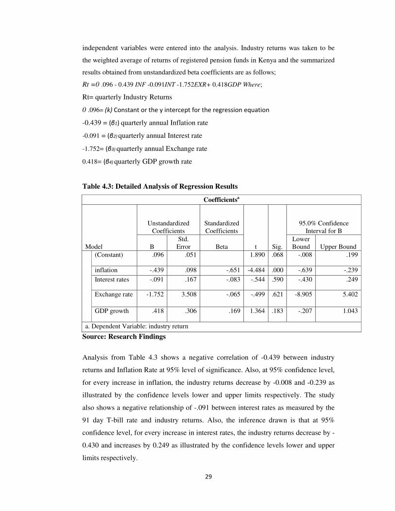
29

independent variables were entered into the analysis. Industry returns was taken to be

the weighted average of returns of registered pension funds in Kenya and the summarized

results obtained from unstandardized beta coefficients are as follows;

Rt =0 .096 - 0.439 INF -0.091INT -1.752EXR+ 0.418GDP Where;

Rt= quarterly Industry Returns

0 .096= (k) Constant or the y intercept for the regression equation

-0.439 = (β1) quarterly annual Inflation rate

-0.091 = (β2) quarterly annual Interest rate

-1.752= (β3) quarterly annual Exchange rate

0.418= (β4) quarterly GDP growth rate

Table 4.3: Detailed Analysis of Regression Results

Coefficientsa

Model

Unstandardized

Coefficients

Standardized

Coefficients

t Sig.

95.0% Confidence

Interval for B

B

Std.

Error Beta

Lower

Bound Upper Bound

(Constant) .096 .051 1.890 .068 -.008 .199

inflation -.439 .098 -.651 -4.484 .000 -.639 -.239

Interest rates -.091 .167 -.083 -.544 .590 -.430 .249

Exchange rate -1.752 3.508 -.065 -.499 .621 -8.905 5.402

GDP growth .418 .306 .169 1.364 .183 -.207 1.043

a. Dependent Variable: industry return

Source: Research Findings

Analysis from Table 4.3 shows a negative correlation of -0.439 between industry

returns and Inflation Rate at 95% level of significance. Also, at 95% confidence level,

for every increase in inflation, the industry returns decrease by -0.008 and -0.239 as

illustrated by the confidence levels lower and upper limits respectively. The study

also shows a negative relationship of -.091 between interest rates as measured by the

91 day T-bill rate and industry returns. Also, the inference drawn is that at 95%

confidence level, for every increase in interest rates, the industry returns decrease by -

0.430 and increases by 0.249 as illustrated by the confidence levels lower and upper

limits respectively.

30

Results from the analysis above show a negative relationship of -1.752 between

exchange rate and industry returns. Also, the inference drawn is that at 95%

confidence level, for every increase in dollar/KES exchange rate, the industry returns

decreases by -8.905 and increases by 5.402 as illustrated by the confidence levels

lower and upper limits respectively. There exists a positive relationship of .418

between industry returns and GDP growth Rate. Also, the inference drawn is that at

95% confidence level, for every increase in GDP rate, the industry returns decrease by

-0.207 and increase by 1.043as illustrated by the confidence levels lower and upper

limits respectively.

4.3.4 Test of Overall Regression Model Significance

The model significance was tested using the F-test. The F value is employed in

testing statistical model that have been aligned to a data set.

Table 4.4: Analysis of Variance (ANOVA)

ANOVAa

Model Sum of

Squares

df Mean Square F Sig.

1

Regression .023 4 .006 8.829 .000b

Residual .020 31 .001

Total .043 35

a. Dependent Variable: industry return)

b. Predictors: (Constant), GDP growth, exchange rate, inflation, interest rates

Source: Research Findings

The F value from Table 4.4 for 36 observations and 4 predictor variables at 5%

significance level is 2.64. The computed F value is 8.829. Therefore since 8.829 >

2.64, there exists a significant relationship between the macro-economic variables and

industry returns.

4.3.5 Model Summary

The R square measure (R2) shows how well the study data fits into the preconceived

model or how a model explains and forecasts future outcomes. It also measures the

goodness of fit of the model and the value expressed as ranging between -1 and 1.

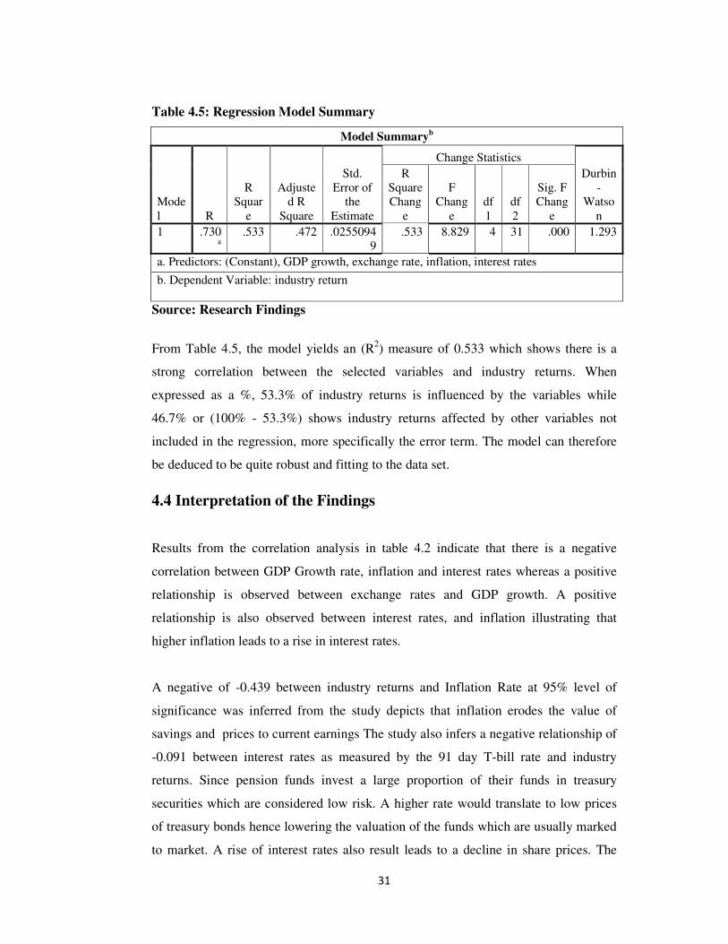
31

Table 4.5: Regression Model Summary

Model Summaryb

Mode

l R

R

Squar

e

Adjuste

d R

Square

Std.

Error of

the

Estimate

Change Statistics

Durbin

-

Watso

n

R

Square

Chang

e

F

Chang

e

df

1

df

2

Sig. F

Chang

e

1 .730a

.533 .472 .0255094

9

.533 8.829 4 31 .000 1.293

a. Predictors: (Constant), GDP growth, exchange rate, inflation, interest rates

b. Dependent Variable: industry return

Source: Research Findings

From Table 4.5, the model yields an (R2) measure of 0.533 which shows there is a

strong correlation between the selected variables and industry returns. When

expressed as a %, 53.3% of industry returns is influenced by the variables while

46.7% or (100% - 53.3%) shows industry returns affected by other variables not

included in the regression, more specifically the error term. The model can therefore

be deduced to be quite robust and fitting to the data set.

4.4 Interpretation of the Findings

Results from the correlation analysis in table 4.2 indicate that there is a negative

correlation between GDP Growth rate, inflation and interest rates whereas a positive

relationship is observed between exchange rates and GDP growth. A positive

relationship is also observed between interest rates, and inflation illustrating that

higher inflation leads to a rise in interest rates.

A negative of -0.439 between industry returns and Inflation Rate at 95% level of

significance was inferred from the study depicts that inflation erodes the value of

savings and prices to current earnings The study also infers a negative relationship of

-0.091 between interest rates as measured by the 91 day T-bill rate and industry

returns. Since pension funds invest a large proportion of their funds in treasury

securities which are considered low risk. A higher rate would translate to low prices

of treasury bonds hence lowering the valuation of the funds which are usually marked

to market. A rise of interest rates also result leads to a decline in share prices. The

32

study also shows negative relationship of -1.752 between exchange rate and industry

returns. The inference is that depreciation of the local currency results in lower returns

for pension funds in Kenya. There exists a positive relationship of 0.418 between

industry returns and GDP growth Rate. The inference is that high GDP rates are a

result of accelerated growth of firms, having a portfolio of firms, post higher returns

during boom periods. Therefore an increase in growth of these firms indicates an

increase in their earnings hence a rise asset prices which in return results to an

increase in shareholders returns.

The computed R

2 was established to be of 0.533 which shows there is a positive and

strong correlation between the selected variables and industry returns. When

expressed as a percentage, 53.3% of industry returns is influenced by the variables

while 46.7% or (100% - 53.3%) shows industry returns affected by other variables not

included in the regression, more specifically the error term. This indicates that the

model is quite reliable in predicting the future effect of selected macroeconomic

variables on industry returns of pension funds in Kenya. The research also established

positive correlation between the dependent and independent variables albeit to

varying degrees. The Durbin Watson test of auto correlation was employed to detect

the presence of autocorrelation among variables. Auto correlation measures the

relationship between variables separated by a time lag. The model was therefore

inferred to be quite robust and fitting to the identified data set. To further test the

models significance and goodness of fit, F test and Analysis of Variance (ANOVA)

were used which showed that from the 36 observations representing every quarter for

a period of 9 years and 4 predictor variables, the F test statistic was 2.64. The

computed F value from the study was 8.829. Since 8.829 > 2.64 hence there exists a

significant relationship between the predictor variables and dependent variable.

33

CHAPTER FIVE

SUMMARY, CONCLUSION AND RECOMMENDATIONS

5.1 Introduction

This chapter draws a summary of the key observations, inferences, findings and

conclusions arising from the study.

5.2 Summary

The aim of this research was to establish the effect of selected macroeconomic

variables on the industry returns of Pension Funds in Kenya. The selected variables

were those perceived by the researcher and supported by previous empirical studies,

to have the highest effect perceived effects on industry returns. These were inflation

rate, interest rates, exchange rate of dollar versus KES and GDP growth rate. Industry

return was taken to be the dependent variable while inflation rate, interest rates,

exchange rate and GDP growth rate were taken to be the independent or predictor

variables. The study also considered an error term as a representative of other non key

variables which had not been included in the model. The study period ranged from

2005 to 2013 within every quarter of a year, therefore consisting of 36 observations.

The data was analyzed using IBM SPSS version 20.

The study established that pension funds’ industry return was heavily influenced by

the selected macroeconomic variables where a negative relationship was inferred

between inflation rate, interest rates and exchange rate whereas GDP had positive

relationship with industry returns. The findings from the study are in tandem with the

earlier estimated hypothesis of existence of a negative relationship between in

inflation and industry returns of pension funds, which is consistent with previous

studies done to study relationship between inflation and share prices where an

increase in the expected future rate of inflation causes a concurrent fall in the ratio of

share Feldestein (1983). Gazi and Mahmudul (2009) had found evidence that interest

rates have a significant negative relationship with share prices. Jorion (1990) found

that for the Investor, changes in exchange rates pose a foreign exchange risk. High

fluctuations in exchange rates can lead to big losses in an investor’s portfolio of

investments due to uncertainty of return on investments.

34

The computed R2 was established to be of 0.533 which shows there is a positive and

strong correlation between the selected variables and industry returns. The research

also established positive correlation between the dependent and independent variables

albeit to varying degrees. The model was therefore inferred to be quite robust and

fitting to the identified data set. To further test the models significance and goodness

of fit, F test and Analysis of Variance (ANOVA) were used which showed that from

the 36 observations representing every quarter for a period of 9 years and 4 predictor

variables, the F test statistic was 2.64. The computed F value from the study was

8.829. Since 8.829 > 2.64 hence there exists a significant relationship between the

predictor variables and dependent variable.

5.3 Conclusion

The study established varying degrees of influence between the independent macro

economic variables selected for the study and industry returns of pension funds. From

the variable with the highest influence to the one with the least, their correlation can

be ranked as inflation rate, interest rate, exchange rate and GDP growth rate. The

objective of the study, which was to establish the effect of selected macroeconomic

variables on the industry returns of Pension funds, was therefore achieved.

A number of studies align to the same hypothesis that there are identifiable effects of

the selected macroeconomic variables on returns though none has been specific to the

returns of Pension funds. Empirical and studies carried out and reviewed in the

empirical literature include; Feldestein (1983), Fama 1981, Chirchir (2013, Olweny

and Omondi (2011) Ross et al (1986) and Illo (2012) among others. They all point out

to existence of a relationship and consistent findings as those established in the study.

5.4 Recommendation for policy

The study established that the selected macroeconomic variables had an effect on the

financial risk. Preparation of the Investment policy should take into account inflation

rate and exchange rate in particular as having the greatest influence on the direction

taken by returns of Pension Funds. All the variables had a correlation with industry

though for some of the variables it was small and not as significant.

35

Inflation, exchange rates and GDP growth rate, in that respective order were

established to be the macroeconomic factors that had the greatest effect on pension

funds’ returns while interest rates showed a negative relationship albeit to a small

extent. Hence, these macro economic variables should be carefully be considered by

industry regulators in the pension industry when setting up limits on asset classes for

pension fund investments. All other stakeholders such as pensioners, pension fund

trustees and administrators should also consider these factors when making decisions

with regard to Pension.

5.5 Limitation of the Study

Due to the constantly evolving macro economic climate, the study may likely be

exceeded by new macroeconomic variables such as unaccounted legal regulations and

taxation instituted by the government thorough the relevant regulatory bodies. They

are key variables with a likely possible impact on performance of the pension fund

industry but whose effect has not been captured in the study.

The study relied on secondary data publicly available in CBK, KNBS which are

government databases due to the scale and cost constraints of the information. The

researcher cannot therefore independently validate the data if it was not prepared

objectively.

The Pension Fund industry is still a developing industry and is governed by the

Retirement Benefits Act which came into operation in 1997. There is therefore a

limitation in terms of information for the prior years when the industry players were

still reorganizing themselves. The last couple of years have also seen a lot of changes

in terms of regulations governing the industry.

5.6 Suggestions for Further Research

Though pension fund’s portfolio managers usually include diverse their investments

to mitigate risk, the classes of investments are limited in terms of proportions that the

funds can invest in a specific class. The investment classes are also not as diverse

hence limiting fund managers to low risk investments. There is therefore a gap as to

the effect of these regulations on the performance of pension funds.

36

Studies also need to be carried out to establish the impact of portfolio management

practices and performance because apart from the macroeconomic variables

identified, there are other key influences on returns of pension funds. There are gaps

in relationship between strategic asset allocation, security selection, and market

timing on pension funds’ returns.

Since the pension industry in Kenya is still developing, further research needs to be

carried in already developed markets to determine the policies adopted by these

markets and how they differ from the Kenyan market. This might result into the

adoption of better market practices and hedging mechanisms.

37

REFERENCES

Beber, A. and Brandt W. (2008), “Resolving Macroeconomic Uncertainty in Stock

and Bond Markets”, Oxford journals

Brinson, GP. , Singer D.B, Gilbert L.B (1991) “Determinants of Portfolio

Performance II: An update”, Financial Analysts Journal

Chirchir, D. (2013), “The relationship between share prices and interest rates:

evidence from Kenya”, School of business, University of Nairobi

Fama E, & R. Fench (1989) “Business conditions and expected returns on stocks and

bonds” The journal of financial economics

Fama, E (1981), “Stock returns, real activity, inflation and money”. American

Economic Review

Feldstein M. (1983), “Inflation and the stock market” University of Chicago Press

Gazi S, & A. Mahmudul A. (2009),“Relationship between Interest Rate and Stock

Price: Empirical Evidence from Developed and Developing Countries”,

International Journal of Business and Management, Vol 4, No. 3, 43-51

Hsing, Y. (2004),“Impacts of Fiscal Policy, Monetary Policy, and Exchange Rate

Policyon Real GDP in Brazil: A VAR Model” Brazilian Electronic Journal of

Economics, 6 (1).

Humpe A. and Macmillian P. (2007), “Can macroeconomic variables explain long

term stock movements?”Centre for Dynamic Macroeconomic Analysis in its

Series, CDMA working paper no. 0720, School of Economics and Finance,

University of St. Andrews.

Kimani D.K & Mutuku C.M. (2013), “Inflation Dynamics on the overall Stock

Market performance” Business Journals

38

Kisaka, S.E, & Mwasaru, A. (2012). “The causal relationship between stock prices

and exchange rates in Kenya”, Research Journal of Finance and Accounting,

Baele L.,Bekaert G, and Inghelbrecht K. (2010), “The determinants of stock and Bond

Return Co movements”, oxford journals

Mmasi B.S (2013), “An investigation of the relationship between interest rate and

inflation in Kenya”, Unpublished MBA project report University of Nairobi

Mutuku N. (2012), “RBA policy briefs 2011/2012” Research & Development

Department Retirement Benefits Authority, retrieved from www.rba.go.ke

Mwai A.M (2013), “The relationship between macroeconomic variables and share

prices of companies listed at the Nairobi securities exchange”, Unpublished

MBA project report, University of Nairobi.

Nai-fu Chen, Richard Roll and Stephen A. Ross, (1986) “Economic forces and the

stock market”, the journal of Business

Njau, D.K (2013) “The effect of selected macroeconomic variables on the financial

performance of private equity firms in Kenya”, unpublished MBA report,

University of Nairobi

Nyamute M.N (1998), “The relationship between NSE index and Major

Macroeconomic Variables”, unpublished MBA project report, University of

Nairobi

Ochieng, D.E, &Owiro A.E, (2012) “The relationship between macroeconomic

variables and stock market performance in Kenya” DBA Africa management

Review

Olweny, T. and Kennedy O. (2011), “The effect of macroeconomic factors on stock

return volatility in The Nairobi Stock Exchange, Kenya”, Business Journal

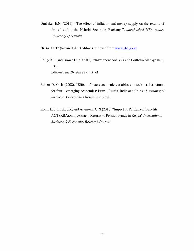
39

Ombaka, E.N, (2011), “The effect of inflation and money supply on the returns of

firms listed at the Nairobi Securities Exchange”, unpublished MBA report,

University of Nairobi

“RBA ACT” (Revised 2010 edition) retrieved from www.rba.go.ke

Reilly K. F and Brown C. K (2011), “Investment Analysis and Portfolio Management,

10th

Edition”, the Dryden Press, USA.

Robert D. G, Jr (2008), “Effect of macroeconomic variables on stock market returns

for four emerging economies: Brazil, Russia, India and China” International

Business & Economics Research Journal

Rono, L. J, Bitok, J.K, and Asamoah, G.N (2010) “Impact of Retirement Benefits

ACT (RBA)on Investment Returns to Pension Funds in Kenya” International

Business & Economics Research Journal

40

APPENDICES

APPENDIX 1: REGISTERED FUND MANAGERS IN KENYA AS

AT JUNE 2014

1. African Alliance Kenya Management Company Limited.

2. Amana Capital Limited.

3. Apollo Asset Management Company Limited

4. Pinebridge Investment East Africa Limited

5. Aureos Kenya Managers Limited

6. British-American Asset Management Managers Limited.

7. CIC Asset Management Company Limited

8. Co-op Trust Investment Services Limited

9. Dry associates Limited

10. Genesis Kenya Investment Management Services Limited.

11. ICEA Asset Management Limited.

12. InvesteQ Capital Limited

13. Madison Asset Management Company Limited

14. Old Mutual Asset Managers (Kenya) Limited.

15. Sanlam Investment Management Kenya Limited.

15. Standard Chartered Investment Services Limited

17. Stanbic Investment Management Services (East Africa) Limited.

18. Zimele Asset Management Company Limited.

19. Jubilee Financial Services

Source: RBA Website

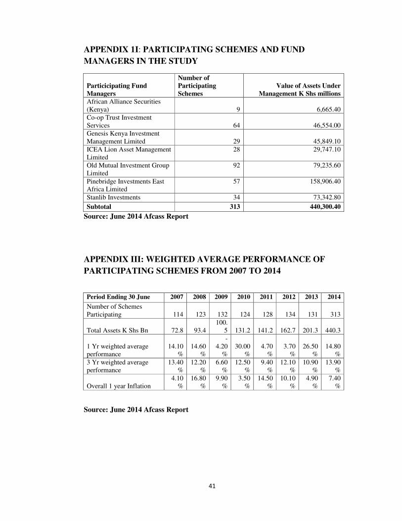
41

APPENDIX 1I: PARTICIPATING SCHEMES AND FUND

MANAGERS IN THE STUDY

Particicipating Fund

Managers

Number of

Participating

Schemes

Value of Assets Under

Management K Shs millions

African Alliance Securities

(Kenya) 9 6,665.40

Co-op Trust Investment

Services 64 46,554.00

Genesis Kenya Investment

Management Limited 29 45,849.10

ICEA Lion Asset Management

Limited

28 29,747.10

Old Mutual Investment Group

Limited

92 79,235.60

Pinebridge Investments East

Africa Limited

57 158,906.40

Stanlib Investments 34 73,342.80

Subtotal 313 440,300.40

Source: June 2014 Afcass Report

APPENDIX III: WEIGHTED AVERAGE PERFORMANCE OF

PARTICIPATING SCHEMES FROM 2007 TO 2014

Period Ending 30 June 2007 2008 2009 2010 2011 2012 2013 2014

Number of Schemes

Participating 114 123 132 124 128 134 131 313

Total Assets K Shs Bn 72.8 93.4

100.

5 131.2 141.2 162.7 201.3 440.3

1 Yr weighted average

performance

14.10

%

14.60

%

-

4.20

%

30.00

%

4.70

%

3.70

%

26.50

%

14.80

%

3 Yr weighted average

performance

13.40

%

12.20

%

6.60

%

12.50

%

9.40

%

12.10

%

10.90

%

13.90

%

Overall 1 year Inflation

4.10

%

16.80

%

9.90

%

3.50

%

14.50

%

10.10

%

4.90

%

7.40

%

Source: June 2014 Afcass Report

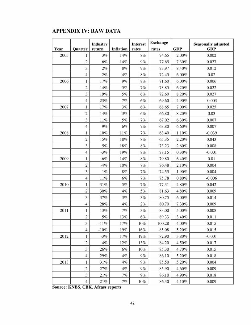
42

APPENDIX IV: RAW DATA

Year Quarter

Industry

return Inflation

Interest

rates

Exchange

GDP

Seasonally adjusted

GDP rates

2005 1 3% 14% 8% 74.65 2.00% 0.002

2 6% 14% 9% 77.65 7.30% 0.027

3 2% 8% 9% 73.97 8.40% 0.012

4 2% 4% 8% 72.45 6.00% 0.02

2006 1 17% 9% 8% 71.60 6.00% 0.006

2 14% 5% 7% 73.85 6.20% 0.022

3 19% 5% 6% 72.60 8.20% 0.027

4 23% 7% 6% 69.60 4.90% -0.003

2007 1 17% 3% 6% 68.65 7.00% 0.025

2 14% 3% 6% 66.80 8.20% 0.03

3 11% 5% 7% 67.02 6.30% 0.007

4 9% 6% 7% 63.80 6.60% 0.007

2008 1 10% 11% 7% 63.40 1.10% -0.039

2 15% 18% 8% 65.35 2.20% 0.043

3 5% 18% 8% 73.23 2.60% 0.008

4 -3% 19% 8% 78.15 0.30% -0.001

2009 1 -6% 14% 8% 79.80 6.40% 0.01

2 -4% 10% 7% 76.48 2.10% 0.004

3 1% 8% 7% 74.55 1.90% 0.004

4 11% 6% 7% 75.78 0.80% -0.006

2010 1 31% 5% 7% 77.31 4.80% 0.042

2 30% 4% 5% 81.63 4.80% 0.009

3 37% 3% 3% 80.75 6.00% 0.014

4 28% 4% 2% 80.70 7.30% 0.009

2011 1 13% 7% 3% 83.00 5.00% 0.008

2 5% 13% 6% 89.33 3.40% 0.011

3 -11% 17% 10% 100.28 4.00% 0.015

4 -10% 19% 16% 85.08 5.20% 0.015

2012 1 -3% 17% 19% 82.90 3.80% -0.001

2 4% 12% 13% 84.20 4.50% 0.017

3 26% 6% 10% 85.30 4.70% 0.015

4 29% 4% 9% 86.10 5.20% 0.018

2013 1 31% 4% 9% 85.50 5.20% 0.004

2 27% 4% 9% 85.90 4.60% 0.009

3 21% 7% 9% 86.10 4.90% 0.018

4 21% 7% 10% 86.30 4.10% 0.009

Source: KNBS, CBK. Afcass reports