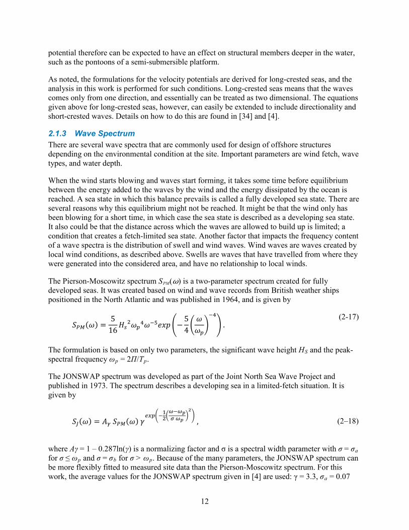
Embed Size (px)
Citation preview
NREL is a national laboratory of the U.S. Department of Energy Office of Energy Efficiency & Renewable Energy Operated by the Alliance for Sustainable Energy, LLC This report is available at no cost from the National Renewable Energy Laboratory (NREL) at www.nrel.gov/publications.
Contract No. DE-AC36-08GO28308
The Effect of Second-Order Hydrodynamics on a Floating Offshore Wind Turbine L. Roald Eidgenössische Technische Hochschule Zürich Laboratory for Energy Conversion
J. Jonkman and A. Robertson National Renewable Energy Laboratory
Technical Report NREL/TP-5000-61452 May 2014
NREL is a national laboratory of the U.S. Department of Energy Office of Energy Efficiency & Renewable Energy Operated by the Alliance for Sustainable Energy, LLC This report is available at no cost from the National Renewable Energy Laboratory (NREL) at www.nrel.gov/publications.
Contract No. DE-AC36-08GO28308
National Renewable Energy Laboratory 15013 Denver West Parkway Golden, CO 80401 303-275-3000 • www.nrel.gov
The Effect of Second-Order Hydrodynamics on a Floating Offshore Wind Turbine L. Roald Eidgenössische Technische Hochschule Zürich Laboratory for Energy Conversion
J. Jonkman and A. Robertson National Renewable Energy Laboratory
Prepared under Task No. WE11.5070
Technical Report NREL/TP-5000-61452 May 2014

NOTICE
This report was prepared as an account of work sponsored by an agency of the United States government. Neither the United States government nor any agency thereof, nor any of their employees, makes any warranty, express or implied, or assumes any legal liability or responsibility for the accuracy, completeness, or usefulness of any information, apparatus, product, or process disclosed, or represents that its use would not infringe privately owned rights. Reference herein to any specific commercial product, process, or service by trade name, trademark, manufacturer, or otherwise does not necessarily constitute or imply its endorsement, recommendation, or favoring by the United States government or any agency thereof. The views and opinions of authors expressed herein do not necessarily state or reflect those of the United States government or any agency thereof.
This report is available at no cost from the National Renewable Energy Laboratory (NREL) at www.nrel.gov/publications.
Available electronically at http://www.osti.gov/scitech
Available for a processing fee to U.S. Department of Energy and its contractors, in paper, from:
U.S. Department of Energy Office of Scientific and Technical Information P.O. Box 62 Oak Ridge, TN 37831-0062 phone: 865.576.8401 fax: 865.576.5728 email: mailto:[email protected]
Available for sale to the public, in paper, from:
U.S. Department of Commerce National Technical Information Service 5285 Port Royal Road Springfield, VA 22161 phone: 800.553.6847 fax: 703.605.6900 email: [email protected] online ordering: http://www.ntis.gov/help/ordermethods.aspx
Cover Photos: (left to right) photo by Pat Corkery, NREL 16416, photo from SunEdison, NREL 17423, photo by Pat Corkery, NREL 16560, photo by Dennis Schroeder, NREL 17613, photo by Dean Armstrong, NREL 17436, photo by Pat Corkery, NREL 17721.
Printed on paper containing at least 50% wastepaper, including 10% post consumer waste.


ii
Acknowledgments First, I wish to thank Dr. Jason Jonkman and Dr. Amy Robertson, my supervisors at NREL, for their support and interest throughout the project. They always found time to discuss my work and help me with any obstacles, and their input and ideas are very much valued. Working with them has allowed me not only to expand my knowledge of wind energy and hydrodynamics, but also to have a lot of fun along the way. I truly appreciate the opportunity to work on this project for my master thesis, and also thank Dr. Jonkman for his help in facilitating my stay at NREL.
I would like to thank my supervisor in Zurich, Dr. Ndaona Chokani, for motivating me and providing input on my work. I am very grateful for Dr. Chokani’s help with the organization of my thesis.
Further, thanks are due Professor Reza S. Abhari—head of the Laboratory for Energy Conversion at ETH Zurich, and my tutor—for his role in my education and for giving me the opportunity to pursue this project at NREL.
Thanks to Jan Muren of 4subsea, Norway, for invaluable input and for introducing me to hydrodynamics and offshore wind technology in the first place.
Many thanks to all the people I have been working with at NREL. Special thanks to Bonnie Jonkman for helping me change FAST to output wave amplitudes, turning my uneasiness about compiling FAST into confidence, and for helping me run my TurbSim cases. Thank you Senu Sirnivas for all the discussions about floating offshore platforms and the oil and gas industry perspective, and for introducing me to John Halkyard of John Halkyard and Associates, whom I also thank for looking into my TLP questions. Thanks to Marco Masciola, for interesting discussions and valuable input—as well as for sharing the WAMIT dongle with me. I also thank Cynthia Szydlek and Beverly Cisneros for solving all formalities regarding my stay at NREL, and Billy Hoffman and Rodd Hamann for creating solutions to all IT problems encountered throughout this work. Thank you Walt Musial, supervisor of the offshore wind energy program, and Fort Felker, the National Wind Technology Center director, for your interest in my project and for allowing me to pursue this opportunity at the NWTC.
Finally, I extend sincere thanks to my friends and family for your support throughout my education. A special thanks to Matthias Thaler, who came all the way from Switzerland to share this experience in Colorado with me.
iii
Acronyms and Abbreviations BEM blade-element / momentum BVP boundary-value problem CoG center of gravity CoB center of buoyancy DOF degree of freedom FAST Fatigue, Aerodynamics, Structures, and Turbulence FFT fast Fourier transform GDF geometric data file IEA International Energy Agency IEC International Electrotechnical Commission JONSWAP Joint North Sea Wave Project KC Keulegan-Carpenter number Re Reynolds number LTF linear transfer function metocean meteorological and oceanographic MIT Massachusetts Institute of Technology NPAN number of body panels NREL National Renewable Energy Laboratory NWTC National Wind Technology Center OC3 Offshore Code Comparison Collaborative O&G oil and gas PARTR partition radius PSD power spectral density QTF quadratic transfer function RAO response amplitude operator SCALE size of the free surface panels TLP tension leg platform UMaine University of Maine WAMIT Wave Analysis at MIT

iv
Nomenclature A, Am amplitude of a regular incident wave, amplitude of
the mth wave with frequency ωm A, Aij Hydrodynamic added-mass matrix, (i,j) component
of hydrodynamic-added-mass matrix A0 water-plane area of the support platform when it is
in its undisplaced position B, Bij Radiation damping matrix, (i,j) component of the
radiation damping matrix C, Cij linear hydrostatic restoring matrix, (i,j) component
of the linear hydrostatic restoring matrix D diameter of structure
PlatformidF ith component of the total external load acting on a
differential element of cylinder in Morison’s equation, other than those loads transmitted from the wind turbine and the weight of the support platform
ViscousidF ith component of the viscous-drag load acting on a
differential element of cylinder in Morison’s equation
dz length of a differential element of cylinder in Morison’s equation
fv vortex shedding frequency fij radiation force coefficient for a force in ith system
degree of freedom, associated with a motions in the jth system degree of freedom
Fext,i wave excitation force in ith system degree of freedom
𝐹𝑒𝑥𝑡,𝑖(1) first-order wave excitation force in ith system degree
of freedom 𝐹𝑒𝑥𝑡,𝑖
(2) second-order wave excitation force in ith system degree of freedom
g gravitational acceleration constant h water depth Hs significant wave height i when not used as a subscript, this is the imaginary
number, 1− κ wave number of an incident wave Kij (i,j) component of the matrix of wave-radiation-
retardation kernels or impulse-response functions of the radiation problem

v
Lij (i,j) component of the matrix of alternative formulations of the wave-radiation-retardation kernels or impulse-response functions of the radiation problem
Mij (i,j) component of the body-mass (inertia) matrix n discrete-time-step counter qj system degree-of-freedom j (without the subscript,
q represents the set of system degrees of freedom) jq first time derivative of system degree-of-freedom j
(without the subscript, q represents the set of first time derivatives of the system degrees of freedom)
jq second time derivative of system degree-of-freedom j (without the subscript, q represents the set of second time derivatives of the system degrees of freedom)
S one-sided power spectral density of the wave elevation per unit time
t simulation time tn discrete-time step Tp peak-spectral period V wind speed x,y,z set of orthogonal axes making up a Cartesian
reference frame xB, yB, zB coordinates of the center of buoyancy xG, yG, zG coordinates of the center of gravity β incident-wave propagation heading direction γ peak shape parameter in the JONSWAP spectrum δij (i,j) component of the Kronecker-Delta function
(i.e., identity matrix), equal to unity when i j= and zero when i j≠
ζ instantaneous elevation of incident waves 𝜁(1) first-order instantaneous elevation of incident waves 𝜁(2) second-order instantaneous elevation of incident
waves ξ platform motion amplitude ξ platform velocity ξ platform acceleration π the ratio of a circle’s circumference to its diameter ρ water density ωj the angular frequency of an incident wave or
frequency of oscillation of mode of motion j of the platform
ωp peak-spectral angular frequency
vi
Executive Summary Offshore winds are generally stronger and more consistent than wind on land. A significant part of the offshore wind resource, however, can be found in deep water—where floating turbines are the only economical means of harvesting the energy. The design of offshore floating wind turbines uses design codes that can simulate the entire coupled system behavior. At the present, most codes include only first-order hydrodynamics, which induce forces and motions varying with the same frequency as the incident waves. Effects due to second- and higher-order hydrodynamics are often ignored in the offshore industry, because the forces induced typically are smaller than the first-order forces. Second-order hydrodynamics, however, do induce forces and motions at the sum-frequency and difference-frequency of the incident waves. Because of the frequency content, second-order hydrodynamics can excite eigenfrequencies of the system, leading to large oscillations that strain the mooring system or to vibrations that cause fatigue damage to the structure. Observations of supposed second-order responses in the DeepCwind model tests performed in spring 2011 sparked interest about how second-order excitation affects wind turbines.
In this report, first- and second-order hydrodynamic analysis used in the offshore oil and gas industry is applied to two different wind turbine concepts—a spar and a tension leg platform (TLP). The results are calculated in the frequency domain using WAMIT, with system matrices derived from linearization of turbine models in FAST. The second-order forces and motions are compared to first-order forces and motions (and also to time-domain response and loads induced by aerodynamic loading as solved by FAST). Further, it presents an analysis of second-order effects in the DeepCwind model tests, including a comparison of the model test results to WAMIT results, an assessment of how wind loading influences the second-order response and an assessment of how second-order effects influence system loads. The comparison to WAMIT results showed relatively large differences. The last part of this report discusses reasons for these differences, as well as important limitations to the second-order calculations in WAMIT.
vii
Table of Contents List of Figures ............................................................................................................................................. x List of Tables ............................................................................................................................................ xiii 1 Introduction ........................................................................................................................................... 1
1.1 Previous Research ............................................................................................................................ 4 1.2 Goals, Objectives, and Scope ........................................................................................................... 5
2 Hydrodynamics ..................................................................................................................................... 5 2.1 Wave Representation ....................................................................................................................... 7
2.1.1 Regular Waves .................................................................................................................... 7 2.1.2 Irregular Waves ................................................................................................................... 9 2.1.3 Wave Spectrum ................................................................................................................. 12
2.2 The Hydrodynamics Problem for Potential Flow .......................................................................... 14 2.2.1 Boundary Conditions ........................................................................................................ 15 2.2.2 Assumptions...................................................................................................................... 16 2.2.3 Perturbation Series ............................................................................................................ 16
2.3 First-Order Hydrodynamics ........................................................................................................... 17 2.3.1 Radiation Problem ............................................................................................................ 18 2.3.2 Diffraction Problem .......................................................................................................... 19 2.3.3 Hydrostatics ...................................................................................................................... 19 2.3.4 Equations of Motion ......................................................................................................... 21
2.4 Second-Order Hydrodynamics ....................................................................................................... 23 2.5 Limitations to the Potential Flow Formulation of the Hydrodynamics Problem ........................... 27
2.5.1 Potential Flow Assumption ............................................................................................... 27 2.5.2 Wave Modeling ................................................................................................................. 28 2.5.3 Viscous Drag..................................................................................................................... 28 2.5.4 Vortex-Induced Vibrations ............................................................................................... 28 2.5.5 Assumption of Small Wave and Motion Amplitudes ....................................................... 29 2.5.6 Higher-Order Effects ........................................................................................................ 29 2.5.7 Short-Crested Seas ............................................................................................................ 29 2.5.8 Interactions Between Columns ......................................................................................... 30
3 Simulation Codes: Capabilities and Limitations ............................................................................. 30 3.1 Fatigue, Aerodynamics, Structures, and Turbulence (FAST) ........................................................ 30 3.2 Wave Analysis at Massachusetts Institute of Technology (WAMIT) ........................................... 32
4 Environmental Conditions ................................................................................................................. 34 5 Spar Analysis ...................................................................................................................................... 37
5.1 Spar Modeling ................................................................................................................................ 37 5.1.1 FAST Model ..................................................................................................................... 37
5.1.1.1 Derivation of System Matrices ................................................................................... 38 5.1.1.2 Derivation of System Eigenfrequencies ..................................................................... 39
5.1.2 WAMIT Model ................................................................................................................. 40 5.1.2.1 First-Order Convergence Tests .................................................................................. 40 5.1.2.2 Second-Order Convergence Tests .............................................................................. 42 5.1.2.3 PARTR Convergence Test ......................................................................................... 43 5.1.2.4 SCALE Convergence Test ......................................................................................... 43 5.1.2.5 NPAN Convergence Test ........................................................................................... 43 5.1.2.6 Comparison of Forces with Existing Literature ......................................................... 45 5.1.2.7 Comparison with OC3-Hywind .................................................................................. 46 5.1.2.8 Comparison with UpWind.......................................................................................... 46
5.1.3 Validity of Potential Flow Assumption ............................................................................ 46 5.2 Comparison of First-Order Time-Domain and Frequency-Domain Solution ................................ 47
viii
5.3 OC3-Hywind WAMIT Results ...................................................................................................... 51 5.3.1 First-Order Results ............................................................................................................ 51 5.3.2 Second-Order Results ....................................................................................................... 55
5.3.2.1 Difference-Frequency Results .................................................................................... 56 5.3.2.1.1 Difference-Frequency Forces............................................................................... 56 5.3.2.1.2 Difference-Frequency Motions—With and Without Mooring Systems .............. 57 5.3.2.1.3 Approximation By Taking Only Quadratic First-Order Terms into Account...... 59
5.3.2.2 Sum-Frequency Results .............................................................................................. 60 5.3.2.2.1 Sum-Frequency Forces ........................................................................................ 60 5.3.2.2.2 Sum-Frequency Motions, With and Without Mooring ........................................ 62 5.3.2.2.3 Approximation by First-Order Interactions ......................................................... 64
5.4 Comparison of First-Order Response and Second-Order Response in Different Sea States ......... 64 5.4.1 Mean-Drift Force .............................................................................................................. 69
5.5 Comparison of Second-Order Effects to Aerodynamic Forces and Response............................... 71 5.5.1 Mean-Drift Force Versus Wind Turbine Thrust ............................................................... 72 5.5.2 Rotor Thrust: Excitation Frequencies ............................................................................... 73 5.5.3 Motion Response: Wind-Induced Compared to Second-Order ........................................ 75
5.5.3.1 Surge Mean Offset ..................................................................................................... 76 5.5.3.2 Surge, Heave, and Pitch Response Spectra ................................................................ 77
6 Tension Leg Platform Analysis ......................................................................................................... 81 6.1 Tension Leg Platform Modeling .................................................................................................... 81
6.1.1 FAST Model ..................................................................................................................... 81 6.1.1.1 Derivation of System Matrices ................................................................................... 82 6.1.1.2 Derivation of System Eigenfrequencies ..................................................................... 82
6.1.2 WAMIT Model ................................................................................................................. 83 6.1.3 Convergence Tests ............................................................................................................ 84
6.1.3.1 First-Order Convergence Tests .................................................................................. 84 6.1.3.2 Second-Order Convergence Tests .............................................................................. 85
6.1.3.2.1 NPAN Convergence Tests ................................................................................... 85 6.1.3.2.2 PARTR Convergence Tests ................................................................................. 86 6.1.3.2.3 SCALE Convergence Tests ................................................................................. 86
6.1.4 Validity of Potential Flow Assumption ............................................................................ 88 6.2 WAMIT Results ............................................................................................................................. 88
6.2.1 First-Order TLP Results .................................................................................................... 88 6.2.2 Second-Order Tension Leg Platform Results ................................................................... 93
6.2.2.1 Difference-Frequency Results .................................................................................... 93 6.2.2.1.1 Force Results ....................................................................................................... 93 6.2.2.1.2 Quadratic Force Results ....................................................................................... 95 6.2.2.1.3 Motion Results for the Moored Tension Leg Platform ........................................ 96
6.2.2.2 Sum-Frequency Results .............................................................................................. 97 6.2.2.2.1 Force Results ....................................................................................................... 97 6.2.2.2.2 Quadratic Force Results ....................................................................................... 99 6.2.2.2.3 Motion Results ................................................................................................... 100
6.3 Comparison of First-Order and Second-Order Forces and Motions in Different Environments . 101 6.4 Comparison to Aerodynamic Forces............................................................................................ 105 6.5 Response from WAMIT Time Series .......................................................................................... 107
7 DeepCwind Wave Tank Test Results and Analysis ...................................................................... 108 7.1 Analysis of DeepCwind Model Test Results for the OC3-Hywind ............................................. 108
7.1.1 Wave-Only Tests ............................................................................................................ 109 7.1.2 Influence of Wind on Second-Order Effects................................................................... 112 7.1.3 The Influence of Second-Order Effects on Turbine Loads and Accelerations ............... 115
ix
7.2 Analysis of Tension Leg Platform Results from DeepCwind Wave Tank Tests ......................... 117 7.2.1 Wave Loading Only ........................................................................................................ 118 7.2.2 Influence of Wind on Second-Order Effects................................................................... 120 7.2.3 Influence of Second-Order Effects on System Loads and Performance ......................... 122
7.3 Differences Between Model Tests and WAMIT Results ............................................................. 125 7.3.1 Differences in the System Dynamics .............................................................................. 126 7.3.2 Inaccuracies in the Model Test ....................................................................................... 126 7.3.3 Viscous Effects ............................................................................................................... 127 7.3.4 Inaccuracies in WAMIT ................................................................................................. 128 7.3.5 Wave Representation ...................................................................................................... 128 7.3.6 Computation of Second-Order Results in WAMIT ........................................................ 130 7.3.7 General Issues ................................................................................................................. 131
8 Summary and Conclusions ............................................................................................................. 131 9 Recommendations for Future Work ............................................................................................... 134 References ............................................................................................................................................... 135 Appendix: FAST Linearization Process ................................................................................................ 138
x
List of Figures Figure 1. The Hywind 2.3 MW floating turbine by Statoil. Photo by Line Roald ..................................... Figure 2. Concepts for floating offshore wind turbines and their ways to achieve stability [15]. ...... 3 Figure 3. Characterization of importance of different hydrodynamic phenomena based on
structure size, wave height, and wave length [8] .............................................................................. 6 Figure 4. Validity ranges of different wave theories; the horizontal axis is a measure of
shallowness and the vertical axis a measure of wave steepness [3]. ............................................ 8 Figure 5. Wave elevation with and without second-order correction .................................................. 11 Figure 6. JONSWAP spectrum with different peak factors ................................................................... 13 Figure 7. Spectrum of wave elevation, with (black) and without (blue) second-order correction, for
a sea state with Hs = 3.66 m and Tp = 9.7 s ...................................................................................... 14 Figure 8. Oscillating platform in still water (left: radiation problem) and fixed-platform in incident
waves (right: diffraction problem) .................................................................................................... 17 Figure 9. Wavelengths in two different water depths ............................................................................ 29 Figure 10. FAST program structure [18]. ................................................................................................ 31 Figure 11. Buoy positions on the northeast U.S. coast ........................................................................ 34 Figure 12. Scatter diagram for buoy 44005—Gulf of Maine; Hs = significant wave height in meters,
Tp = peak spectral period in seconds............................................................................................... 35 Figure 13. Scatter diagram for buoy 44008—Nantucket; Hs = significant wave height in meters, Tp
= peak spectral period in seconds .................................................................................................... 35 Figure 14. Relations between wind speed and wave height, from different sources; blue: data from
reference site [15], light blue: data for fully developed sea [41], black: representative annual occurrences in the North Atlantic [26], green: interpolated data used for further analysis. ...... 36
Figure 15. Mesh with 931 panels ............................................................................................................. 41 Figure 16. Convergence test for hydrodynamic damping in heave; the black line shows the results
using 9,315 body panels (NPAN = 9,315), the red crosses are the 4,035-panel results, the blue dots show the 931-panel results, and the green triangles are the 195-panel results .................. 42
Figure 17. Convergence test results for surge (left), heave (middle), and pitch (right) .................... 45 Figure 18. Exiting force coefficients of OC3-Hywind from convergence tests .................................. 46 Figure 19. Surge displacement [m] ......................................................................................................... 50 Figure 20. Pitch displacement [deg] ....................................................................................................... 50 Figure 21. Heave displacement [m] ......................................................................................................... 51 Figure 22. Added mass coefficients for OC3 Hywind ........................................................................... 52 Figure 23. Radiation damping for OC3 Hywind...................................................................................... 53 Figure 24. First-order wave excitation forces for OC3 Hywind ............................................................ 53 Figure 25. Translational RAOs for the OC3 Hywind .............................................................................. 54 Figure 26. Detail of RAO magnitudes ...................................................................................................... 55 Figure 27 Rotational RAOs for OC3 Hywind .......................................................................................... 55 Figure 28. Difference-frequency force QTFs; upper part shows force QTFs vs. ω1 and ω2, lower
part shows force QTF vs. difference-frequency (ω1 – ω2), for (from left) surge, heave, and pitch ..................................................................................................................................................... 56
Figure 29. Motion RAOs for a freely floating structure; upper part: 3D motion QTFs, lower part: motion QTFs vs. difference-frequency motion QTFs for (from left to right) surge, heave, and pitch ..................................................................................................................................................... 58
Figure 30. Motion RAOs for a moored structure; the upper part shows three-dimensional motion QTFs; lower part shows motion QTFs vs. difference-frequency motion QTFs. From left to right: surge, heave, and pitch ........................................................................................................... 59
Figure 31. QTFs for the difference-frequency quadratic force for (from left to right) surge, heave, and pitch .............................................................................................................................................. 60
Figure 32. Sum-frequency force QTFs; the upper part shows the contour plots of the three-dimensional QTFs; the lower part shows the QTF plotted against sum-frequency. From left to right: Surge, heave, and pitch ........................................................................................................... 61
Figure 33. Sum-frequency motion QTFs for a freely floating system; the upper part shows QTF magnitude vs. ω1 and ω2, the lower part shows QTF vs. sum-frequency. From left to right: Surge, heave, and pitch ..................................................................................................................... 62
xi
Figure 34. Sum-frequency motion QTFs with mooring system; the upper part shows QTF magnitude vs. ω1 and ω2, the lower part shows QTF vs. sum-frequency. From left to right: Surge, heave, and pitch ........................................................................................................... 63
Figure 35. Sum-frequency force QTF including only the contribution from first-order quadratic interactions. From left: Surge, heave, and pitch ............................................................................. 63
Figure 36. First-order and second-order force coefficients (top) and motion coefficients (bottom), dimensionalized by the sea state Hs = 1.4 m and Tp = 6.5 s; ......................................................... 65
black line: first-order, red crosses: difference-frequency, blue crosses: sum-frequency ................ 65 Figure 37. First-order and second-order force coefficients (top) and motion coefficients (bottom)
for the sea state Hs = 1.4 m and Tp = 6.5 s; second-order contributions at a given frequency are summed and shown for 15 realizations of the sea state (black line: first-order, green crosses/red line: difference-frequency single/mean, cyan crosses/blue line: sum-frequency single/mean) ........................................................................................................................................ 67
Figure 38. First-order and second-order force coefficients (top) and motion coefficients (bottom) for the sea state Hs = 3.66 m and Tp = 9.7 s ..................................................................................... 68
Figure 39. First-order and second-order force coefficients (top) and motion coefficients (bottom) for the sea state Hs = 9.14 m and Tp = 13.6 s ................................................................................... 68
Figure 40. Mean-drift force coefficients for the OC3 Hywind ............................................................... 69 Figure 41. Mean-drift force for the sea states in listed in Table 5. From left to right: Mean-drift
force vs significant wave height, mean-drift force vs peak-spectral period, mean-drift force vs. wave steepness .................................................................................................................................. 70
Figure 42. Mean-drift force and mean wind turbine thrust in cases with operating turbine ................. Figure 43. Mean-drift force and mean turbine thrust in cases with idling turbine ................................. Figure 44. Power spectral density of turbine thrust for a low sea state (Hs = 1.4 m, Tp = 6.5 s, wind
speed = 10.5 m/s) ................................................................................................................................ 74 Figure 45. Power spectral density of turbine thrust for a moderate sea state (Hs = 3.66 m, Tp = 9.7
s, wind speed = 17.6 m/s)................................................................................................................... 75 Figure 46. Power spectral density of turbine thrust for a high sea state (Hs = 9.14 m, Tp = 13.6 s,
wind speed = 35.1 m/s)....................................................................................................................... 75 Figure 47. Surge mean offset ................................................................................................................... 76 Figure 48. Pitch mean offset .................................................................................................................... 77 Figure 49. Surge response in different environmental conditions; the left side shows FAST results,
the right side shows WAMIT results ................................................................................................. 78 Figure 50. Heave response in different environmental conditions; left side: FAST results, right
side: WAMIT results ........................................................................................................................... 79 Figure 51. Pitch response in different environmental conditions; left side: FAST results, right
side: WAMIT results ........................................................................................................................... 80 Figure 52. Heave exciting force coefficients for different discretizations .......................................... 85 Figure 53. Chosen TLP discretization with 4,922 panels ...................................................................... 87 Figure 54. Free-surface discretization with SCALE = 3 and PARTR = 100 ......................................... 87 Figure 55. Keulegan-Carpenter number for the UMaine TLP in different regular waves; the
calculation assumes a constant diameter; at the bottom of the column, where the diameter is larger, the KC number in reality would be smaller.......................................................................... 88
Figure 56. Added-mass coefficients for the UMaine TLP ..................................................................... 89 Figure 57. Hydrodynamic damping coefficients for the UMaine TLP .................................................. 90 Figure 58. Exciting force coefficients for the UMaine TLP ................................................................... 91 Figure 59. Motion RAOs for translational modes of the UMaine TLP .................................................. 92 Figure 60. Detail of motion RAOs for translational modes of the UMaine TLP .................................. 92 Figure 61. Motion RAOs for the rotational modes of the UMaine TLP ................................................ 93 Figure 62. Difference-frequency total force QTFs for UMaine TLP for (from left to right) surge,
heave, and pitch; upper part shows force QTF plotted against incident wave frequencies; lower part shows force QTFs plotted for constant sum-frequency against difference-frequency of incident wave pairs ........................................................................................................................ 94
Figure 63. Difference-frequency quadratic force QTFs for UMaine TLP for (from left to right) surge, heave, and pitch; the upper part shows force QTF plotted against incident wave frequencies; the lower part shows force QTFs plotted against difference-frequency of incident wave pairs 95

xii
Figure 64. Difference-frequency motion QTFs for UMaine TLP for (from left to right) surge, heave, and pitch; the upper part shows motion QTF plotted against incident wave frequencies; the lower part shows motion QTFs plotted for constant sum-frequency against the difference-frequency of incident wave pairs ...................................................................................................... 97
Figure 65. Sum-frequency total force QTFs for UMaine TLP for(from left to right) surge, heave, and sway; the upper part shows force QTF plotted against incident wave frequencies; the lower part shows force QTFs plotted for constant sum-frequency against the difference-frequency of incident wave pairs ........................................................................................................................ 98
Figure 66. Sum-frequency quadratic force QTFs for UMaine TLP for (from left to right) surge, heave, and pitch; the upper part shows the force QTF plotted against incident wave frequencies; the lower part shows force QTFs plotted against sum-frequency of incident wave pairs ..................................................................................................................................................... 99
Figure 67. Sum-frequency motion QTFs of the UMaine TLP for (from left to right) surge, heave, and sway; the upper part shows motion QTF plotted against incident wave frequencies; the lower part shows motion QTFs plotted against sum-frequency of incident wave pairs ..................... 100
Figure 68. First-order and second-order force (upper half) and motion (lower half) coefficients for the sea state Hs = 1.4 m and Tp = 6.5 s. Black line: First-order forces/motions, Blue crosses: Sum-frequency forces/motions for 15 realizations, with blue line showing the mean. Green crosses: Difference-frequency forces/motions for 15 realizations, with red line showing the mean. ................................................................................................................................................. 102
Figure 69. First-order and second-order force (upper part) and motion (lower part) coefficients for the sea state Hs = 3.66 m and Tp = 9.7 s ........................................................................................ 103
Figure 70. First-order and second-order force (upper part) and motion (lower part) coefficients for the sea state Hs=9.14 m and Tp = 13.6 s ........................................................................................ 103
Figure 71. Mean-drift force coefficients in surge for the UMaine TLP ............................................... 104 Figure 72. Mean-drift force against significant wave height .............................................................. 105 Figure 73. Mean-drift force against peak-spectral frequency ............................................................. 105 Figure 74. Mean-drift force against average steepness ...................................................................... 105 Figure 75. Mean-drift force and mean wind turbine thrust for the cases with an operating turbine106 Figure 76. Mean-drift force and mean wind turbine thrust for the cases with an idling turbine .... 106 Figure 77. Motion response from WAMIT time series in different sea states; left: low sea state
(Hs = 1.4 m, Tp = 6.5 s); middle: moderate sea state (Hs = 3.66 m, Tp = 9.7 s); right: high sea state (Hs = 9.14 m, Tp = 13.6 s); upper: surge, middle: heave, bottom: pitch ............................. 108
Figure 78. Power spectral density of wave elevation for wave-only cases ...................................... 111 Figure 79. Power spectral density of surge motion at the waterline for the wave-only cases ....... 111 Figure 80. Power spectral density of the heave motion at the waterline for the wave-only cases 111 Figure 81. Power spectral density of the pitch motion for the wave-only cases ............................. 111 Figure 82. Response (at waterline) of the spar configuration in three different sea states with
different wind conditions; left: normal operating sea state (Hs = 2 m, Tp = 7.5 s), middle: 1-year storm (Hs = 7.1 m, Tp = 12.1s ), right: 100-year storm (Hs = 10.5 m, Tp = 14.3 s); top to bottom: surge, heave, and pitch response (at waterline) ........................................................................... 114
Figure 83. Tower-bending moment for the spar in three different sea states with different wind conditions, measured in the DeepCWind wave tank tests .................................................................
Figure 84. Nacelle acceleration of the spar in three different sea states with different wind conditions, measured in the DeepCWind wave tank tests .................................................................
Figure 85. Power spectral density of the wave elevation in the wave-only DeepCwind tests ........ 119 Figure 86. Power spectral density of the surge motion at waterline for the wave-only cases in the
DeepCwind model tests. .................................................................................................................. 119 Figure 87. Power spectral density of the heave motion at waterline for the wave-only cases in the
DeepCwind model tests ................................................................................................................... 119 Figure 88. Power spectral density of the pitch response for the wave-only cases in the DeepCwind
model tests ........................................................................................................................................ 119 Figure 89. Response of the TLP configuration in three different sea states with different wind
conditions for (from left to right) normal operating sea state (Hs = 2 m, Tp = 7.5 s), 1-year storm (Hs = 7.1 m, Tp = 12.1 s), and 100-year storm (Hs = 10.5 m, Tp = 14.3 s); and showing (from top to bottom) surge, heave, and pitch response (at waterline) ........................................................ 121
xiii
Figure 90. Nacelle accelerations measured for the TLP configuration in the DeepCwind model-scale tests ......................................................................................................................................... 123
Figure 91. Tower-bending moment measured for the TLP configuration in the DeepCwind model-scale tests ......................................................................................................................................... 123
Figure 92. Arrangement of tendons for the TLP .................................................................................. 124 Figure 93. Power spectral density of measured tension in tendon 2 for the DeepCWind model tests125 Figure 94. Photo of the TLP during the wave tank tests ..................................................................... 127 Figure 95. Power spectral density (PSD) of wave elevation for the WAMIT time series (Hs = 3.66 m,
Tp = 9.7 s) .......................................................................................................................................... 129 Figure 96. Power spectral density of wave elevation from the wave tank (wave-only tests) .......... 129 Figure 97. Roll RAO for a TLP configuration calculated with a flexible turbine (“FAST”) and with a
rigid turbine (“WAMIT” and “FAST Rigid Turbine”) [28]. ............................................................. 131
List of Tables Table 1. Environmental Conditions Selected for Investigation ............................................................ 37 Table 2. Main Properties of the OC3-Hywind Turbine ........................................................................... 38 Table 3. Eigenfrequencies of the OC3 Hywind with Rigid Tower......................................................... 39 Table 4. Eigenfrequencies of the OC3 Hywind with Flexible Tower .................................................... 39 Table 5. Sea States for which the mean-drift force is computed ......................................................... 70 Table 6. Main Properties of the University of Maine Tension Leg Platform ........................................ 81 Table 7. Platform Eigenfrequencies of the TLP Configuration Without (Left) and With (Right) Tower
DOFs Included In the FAST Model .................................................................................................... 83 Table 8. Comparison of Difference-Frequency Peak Values to First-Order Peak Values ................. 95 Table 9. Comparison of Peak Values of Difference-Frequency Quadratic QTF to Peak Values of the
Total Difference-Frequency Force QTF ............................................................................................ 96 Table 10. Comparison of Sum-Frequency Peak Values to First-Order Peak Values ......................... 98 Table 11. Comparison of Sum-Frequency Quadratic Force QTFs to Total Sum-Frequency Force
QTFs ..................................................................................................................................................... 99 Table 12. Eigenfrequencies of Spar in the Wave Tank Tests and in WAMIT .................................... 109 Table 13. Test Matrix for the DeepCwind Wave Tank Tests [10]. ....................................................... 109 Table 14. Wind Conditions Used in the Wave Tank Tests .................................................................. 112 Table 15. Eigenfrequencies of the TLP in the Wave Tank Test and in WAMIT ................................. 117
1
1 Introduction Every part of an advanced society depends on a reliable supply of electrical power. Traditionally, this energy has been supplied by non-renewable fossil fuels such as oil, natural gas, coal, and nuclear materials. Facing climate change and depletion of natural resources, the only sustainable option is to “decarbonize” the energy supply by switching to renewable energy. Wind energy generation has been growing quickly for more than a decade, and wind now is the second-largest renewable energy sector after hydropower [12]. Generation capacity has increased from 24 GW in 2001 to 240 GW today, with 2011 being a record year with 42 GW of new installed capacity [42]. Wind energy not only provides clean electricity, it also generates local jobs and increases the security of future supply by decreasing the dependence on fossil fuels and the countries that provide them.
In many parts of the world, the wind resource available on land is located far away from urban load centers, in regions where vacant land is scarce, or in areas that cannot be used for wind parks due to environmental protection. In Europe, the need to place wind turbines where they do not disturb people or wildlife has led to the construction of offshore wind parks. Other reasons for building offshore turbines are that the offshore wind resource generally is characterized by stronger and more consistent winds, and that the resource often is found close to major load centers. The trade-off is higher investment cost, more complicated construction, and more expensive maintenance. Nevertheless, the installed offshore wind power capacity in Europe is now 3,813 MW, with an additional 2,375 MW under construction and projects accounting for 2,910 MW being prepared [7].
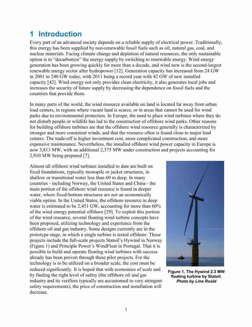
Almost all offshore wind turbines installed to date are built on fixed foundations, typically monopile or jacket structures, in shallow or transitional water less than 60 m deep. In many countries - including Norway, the United States and China - the main portion of the offshore wind resource is found in deeper water, where fixed-bottom structures are not an economically viable option. In the United States, the offshore resource in deep water is estimated to be 2,451 GW, accounting for more than 60% of the wind energy potential offshore [29]. To exploit this portion of the wind resource, several floating wind turbine concepts have been proposed, utilizing technology and experience from the offshore oil and gas industry. Some designs currently are in the prototype stage, in which a single turbine is tested offshore. These projects include the full-scale projects Statoil’s Hywind in Norway (Figure 1) and Principle Power’s WindFloat in Portugal. That it is possible to build and operate floating wind turbines with success already has been proven through these pilot projects. For the technology is to be utilized on a broader scale, the cost must be reduced significantly. It is hoped that with economies of scale and by finding the right level of safety (the offshore oil and gas industry and its verifiers typically are accustomed to very stringent safety requirements), the price of construction and installation will decrease.
Figure 1. The Hywind 2.3 MW floating turbine by Statoil.
Photo by Line Roald

2
Designing, building, and maintaining offshore wind parks requires knowledge about both wind turbines and the marine environment in which they are to function. Important tools for finding the optimal design for a floating turbine are design codes that allow for a coupled simulation of the turbine. A coupled simulation in this case means a time-domain simulation of the entire turbine system, including aerodynamics, hydrodynamics, structural elasticity, and the turbine control system. The codes used for offshore simulations are typically codes which were created for land-based turbines, and augmented with a hydrodynamic module to account for wave interactions, platform motions, and the mooring system later on. The codes that were verified through the OC3 code-to-code comparison project include (among others) FAST by NREL, GH Bladed by GL Garrad Hassan, and HAWC2/SIMO and Riflex by Risoe/MarinTek.
The hydrodynamic modules of most floating wind design codes are limited to calculations using first-order radiation and diffraction, Morison’s equation, or a combination of both. Morison’s equation is a rather empirical but commonly used equation for wave loading on slender structures. It includes viscous drag but uses a long wavelength approximation for the scattering of incident waves. The radiation and diffraction approach incorporates wave reflection and scattering, but ignores all viscous effects by assuming potential flow. Assuming a small wave slope, the radiation and diffraction problem is expanded using a perturbation series, and is split into a first-order, a second-order, and a higher-order part. These parts then can be solved separately. In the offshore industry, it is common to solve only the first-order problem and neglect all other terms. This approach has been adopted for the wind turbine simulation codes mentioned above, and is the reason why only first-order radiation and diffraction has yet been included in the codes. Due to the linearity of the problem, the forces and motions from the first-order problem oscillate at the same frequency as the incident waves.
The second-order terms of the perturbation series form the second-order hydrodynamic problem, which is the topic of interest for this report. The second-order problem addresses interactions between two harmonically oscillating components, resulting in forces and motions at the sum-frequency and difference-frequency of the incident waves. The second-order forces typically are orders of magnitude smaller than the first-order forces, which is why they often are ignored. They can however cause problems due to their frequency content. Offshore structures normally are designed such that their eigenfrequencies are outside the range at which first-order incident waves contain significant energy—above or below 0.25 to 1.25 rad/s (periods of 5 to 25 s). The sum-frequency and difference-frequency forces can excite these eigenfrequencies, and if the damping of the eigenmodes is sufficiently small, the result can be large oscillations or problematic vibrations.
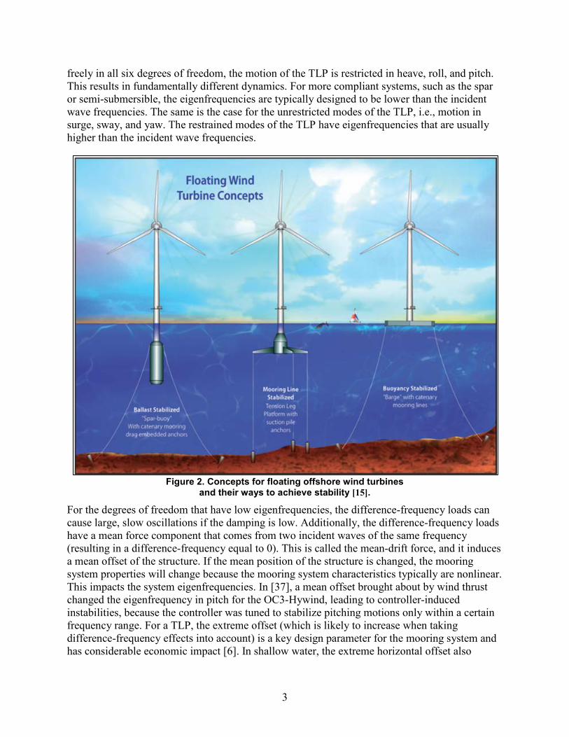
The effects of the second-order forces depend heavily on system eigenfrequencies and floater geometry, and should therefore be studied for a number of different structures. The three main concepts for floating wind turbine platforms are a spar buoy, a semi-submersible, and a tension leg platform (TLP), with some hybrid versions (Figure 2). The main difference between the concepts is the method used to achieve stability. The spar buoy is stabilized by a low center of gravity and the semi-submersible mainly by a large waterline area. The TLP relies on the combination of excess buoyancy and its mooring system for stability. Excess buoyancy of the platform keeps the tension legs (typically called “tendons”) under tension, leading to a very stiff mooring system with high restoring coefficients in heave, roll, and pitch. While the spar and the semi-submersible usually are moored in a manner that allows the structures to move relatively
3
freely in all six degrees of freedom, the motion of the TLP is restricted in heave, roll, and pitch. This results in fundamentally different dynamics. For more compliant systems, such as the spar or semi-submersible, the eigenfrequencies are typically designed to be lower than the incident wave frequencies. The same is the case for the unrestricted modes of the TLP, i.e., motion in surge, sway, and yaw. The restrained modes of the TLP have eigenfrequencies that are usually higher than the incident wave frequencies.
Figure 2. Concepts for floating offshore wind turbines and their ways to achieve stability [15].
For the degrees of freedom that have low eigenfrequencies, the difference-frequency loads can cause large, slow oscillations if the damping is low. Additionally, the difference-frequency loads have a mean force component that comes from two incident waves of the same frequency (resulting in a difference-frequency equal to 0). This is called the mean-drift force, and it induces a mean offset of the structure. If the mean position of the structure is changed, the mooring system properties will change because the mooring system characteristics typically are nonlinear. This impacts the system eigenfrequencies. In [37], a mean offset brought about by wind thrust changed the eigenfrequency in pitch for the OC3-Hywind, leading to controller-induced instabilities, because the controller was tuned to stabilize pitching motions only within a certain frequency range. For a TLP, the extreme offset (which is likely to increase when taking difference-frequency effects into account) is a key design parameter for the mooring system and has considerable economic impact [6]. In shallow water, the extreme horizontal offset also
4
impacts the air gap of the TLP, which is reduced due to a set-down associated with the horizontal movement. The air gap required to keep the turbine rotor out of the waves under any condition therefore must be increased for a larger extreme offset. This influences the required tower height, the system dynamics, and the cost of the turbine. Even though difference-frequency forces cause mean forces and slow oscillations, the rotor thrust on a turbine might have the same effect. The mean thrust that caused the horizontal offset observed in [37] might be of much greater influence than the second-order hydrodynamics. Therefore, a comparison of the second-order effects and the aerodynamic forces is part of the scope of this work.
For a system with high eigenfrequencies, the sum-frequency effects called springing become important. In [38] it is stated that the sum-frequency responses are non-Gaussian, and are determined both by the excitation QTF and the wave damping. The greatest responses typically are generated by groups of short wave components with wave periods “tuned” to half the eigenfrequency of the TLP. Ref. [22] also says that the most important contributions come from short wave pairs where in which both waves have similar wave periods, because the waves tend to cancel each other if the frequency difference gets too large. This means that the largest responses are generated in moderate (frequently occurring) sea states. These descriptions suit the observations of oil and gas TLPs. The sum-frequency effects are known to have significant impact on the fatigue of TLP tendons due to increased loads per cycle and the high number of cycles [32], [22]. The sum-frequency forces also can lead to excitation of eigenmodes in other parts of the structure. Of special concern for wind turbines is the eigenfrequency of the tower. In the UMaine TLP model-scale tests, a coupling between the pitch and tower natural frequencies led to high responses of both the platform and the tower, as reported in [9] and [10]. It also is expected that the sum-frequency forces can induce resonant response in the tower for other platforms.
1.1 Previous Research Difference-frequency effects on offshore structures have been studied since the 1960s, to understand the large scale, slow oscillations induced by difference-frequency forces. The mean-drift forces have been of interest to ocean engineers for an equally long time. The complete formulation of the second-order problem and the computational power needed to solve it was developed during the ’80s, partly in reaction to the need for prediction of sum-frequency loads and responses that were observed on the first TLP platforms. Second- and higher-order hydrodynamic effects, and the development and validation of programs to simulate them, were subjects of extensive research in the early 1990s and still remain active research topics today.
There are very few previous studies applying second-order theory to floating wind turbines. A paper from the UpWind project [26] provides a summary of the theory of second-order hydrodynamics, and results for first- and second-order hydrodynamic coefficients for the OC3 Hywind and a semisubmersible. This work also includes short timeseries of excitation forces and motions in different regular and irregular waves. Agarwal [2] looks at second-order effects on a monopile structure in shallow water, and uses second-order wave kinematics in combination with Morison’s equation to compare linear with non-linear effects. This approach works well as long as the structures are bottom-mounted slender cylinders, but is less accurate for more general structures. In the DeepCwind model tests performed at the MARIN wave basin in Wageningen, Holland, second-order effects were thought to have been observed, as reported in [9] and [10].
5
The significance of these effects inspired new interest in the loads and responses of floating wind turbines that are induced by second-order hydrodynamics, and is one of the reasons for the choice of topic for this report.
1.2 Goals, Objectives, and Scope The task of this work is to apply second-order analysis commonly used in the offshore oil and gas industry to two different wind turbine concepts. The first concept is the OC3-Hywind, a spar buoy concept based on Statoil’s Hywind design and modified by NREL for use in the OC3 project. The second concept is the DeepCwind TLP designed by the University of Maine. The objectives are:
• to gain general insight in the field of second-order hydrodynamics and the implications for floating wind turbines
• to analyze and draw conclusions from the spar and TLP results that give an indication of if/when second-order hydrodynamics are important for floating offshore wind turbines
• to provide a pre-study for the possible implementation of second-order hydrodynamics in FAST.
2 Hydrodynamics The interactions between a floating platform and the water that surrounds it are vitally important to the design of such structures. The determination of loads and motions caused by these interactions is the main subject of the field of marine hydrodynamics. The hydrodynamics can be split into two parts: The influence of fluid motions such as current or waves on the structure, and the influence of the moving structure on the water, which leads to generation of waves. Hydrostatics also must be accounted for to include effects of buoyancy and hydrostatic restoring.
Hydrodynamic loading usually is calculated in terms of integrated dynamic pressure over the wetted surface of the structure. The total forces include contributions from added mass, linear damping (from wave radiation), non-linear drag (from viscosity), buoyancy (hydrostatic restoring), and forces due to both undisturbed and scattered1 incident waves.
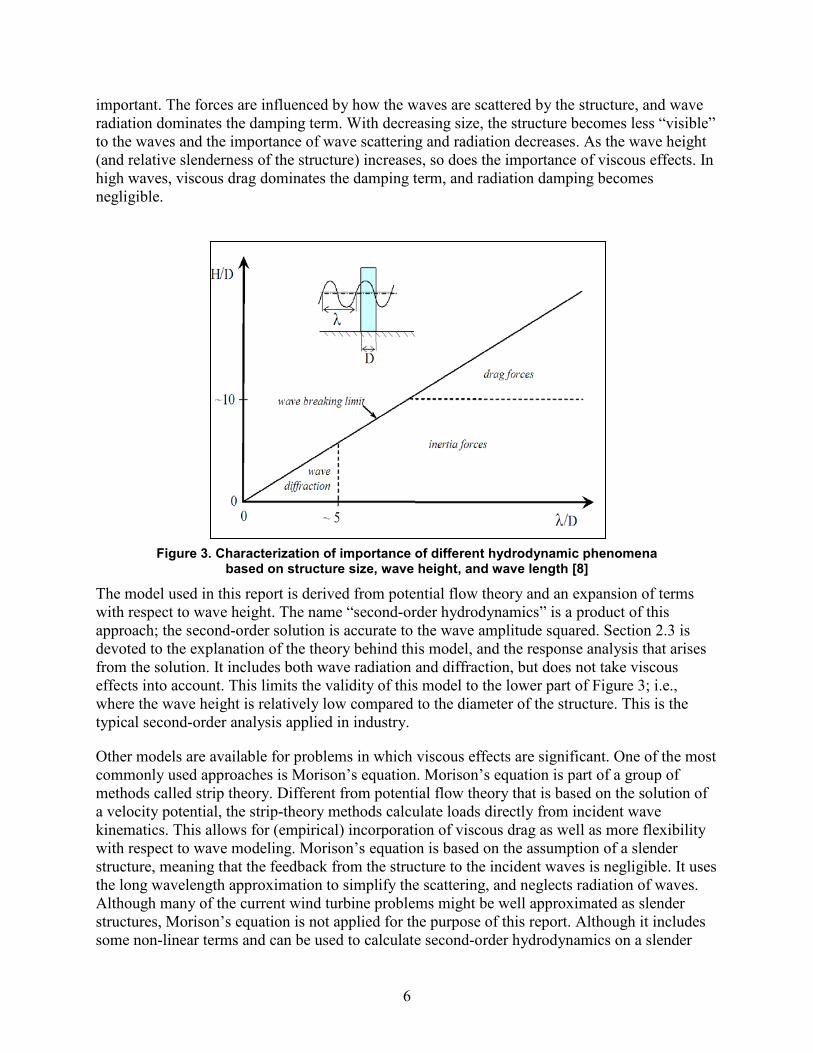
Hydrodynamics is based on the Navier Stokes equations, as all fluid-dynamic problems. To be able to solve practical problems, the mathematical descriptions must be simplified based on assumptions specific to the field of offshore hydrodynamics. The hydrodynamic models commonly used in the offshore industry are therefore all based on assumptions that limit their range of validity. The choice of an appropriate model is important, and depends on parameters such as the characteristic size of the structure and the wave length and wave height of the incident waves. Figure 3 [8] shows what forces are important in different flow regimes. When the size of the structure is large compared to the wave length, wave diffraction and radiation are 1 In this report, the term “scattering” is used for forces due to waves that are reflected by a (fixed) structure, and “diffraction” is used for the total forces experienced by a fixed structure, e.g., due to both scattered and undisturbed waves. This definition is commonly used, but there are many texts that swap the definitions of “scattering” and “diffraction.”
6
important. The forces are influenced by how the waves are scattered by the structure, and wave radiation dominates the damping term. With decreasing size, the structure becomes less “visible” to the waves and the importance of wave scattering and radiation decreases. As the wave height (and relative slenderness of the structure) increases, so does the importance of viscous effects. In high waves, viscous drag dominates the damping term, and radiation damping becomes negligible.
Figure 3. Characterization of importance of different hydrodynamic phenomena based on structure size, wave height, and wave length [8]
The model used in this report is derived from potential flow theory and an expansion of terms with respect to wave height. The name “second-order hydrodynamics” is a product of this approach; the second-order solution is accurate to the wave amplitude squared. Section 2.3 is devoted to the explanation of the theory behind this model, and the response analysis that arises from the solution. It includes both wave radiation and diffraction, but does not take viscous effects into account. This limits the validity of this model to the lower part of Figure 3; i.e., where the wave height is relatively low compared to the diameter of the structure. This is the typical second-order analysis applied in industry.
Other models are available for problems in which viscous effects are significant. One of the most commonly used approaches is Morison’s equation. Morison’s equation is part of a group of methods called strip theory. Different from potential flow theory that is based on the solution of a velocity potential, the strip-theory methods calculate loads directly from incident wave kinematics. This allows for (empirical) incorporation of viscous drag as well as more flexibility with respect to wave modeling. Morison’s equation is based on the assumption of a slender structure, meaning that the feedback from the structure to the incident waves is negligible. It uses the long wavelength approximation to simplify the scattering, and neglects radiation of waves. Although many of the current wind turbine problems might be well approximated as slender structures, Morison’s equation is not applied for the purpose of this report. Although it includes some non-linear terms and can be used to calculate second-order hydrodynamics on a slender
7
cylinder by considering second-order wave kinematics in the incoming waves, it does not allow for proper determination of second-order force contributions on other types of structures. Note also that the definition of slender must be reconsidered in the presence of second-order waves, as the involved wave lengths are significantly shorter.
To describe the interactions between structure and waves, a mathematical description of the waves must be provided. Therefore, an overview of different wave models and their range of validity is presented. The first- and second-order incident wave potentials are presented along with the generalization of linear regular waves to an irregular sea state to provide a basis for description of first- and second-order loads in subsequent sections. The following section is based on [4], [8], [23] and [34] unless another source is cited.
2.1 Wave Representation Ocean waves are of irregular nature, and have random height, shape, length, and propagation speeds. To determine the wave loading and motion response of an offshore structure, engineers mainly rely on two different types of wave descriptions: Deterministic, regular waves of a given wave length, wave height, and wave period; and random, irregular sea states defined by a wave spectrum.
2.1.1 Regular Waves Regular waves often are used to simulate extreme waves or to gain information about the behavior of the system at a given incident wave frequency. Important parameters for a regular wave include the following.
• wave period, T [s]
• wave length, λ [m]
• wave angular frequency, ω = 2Π/T[rad/s]
• wave number, κ = 2Π/λ [1/m]
• wave height, H [m]
• wave crest height, AC [m]
• wave trough depth, AT [m]
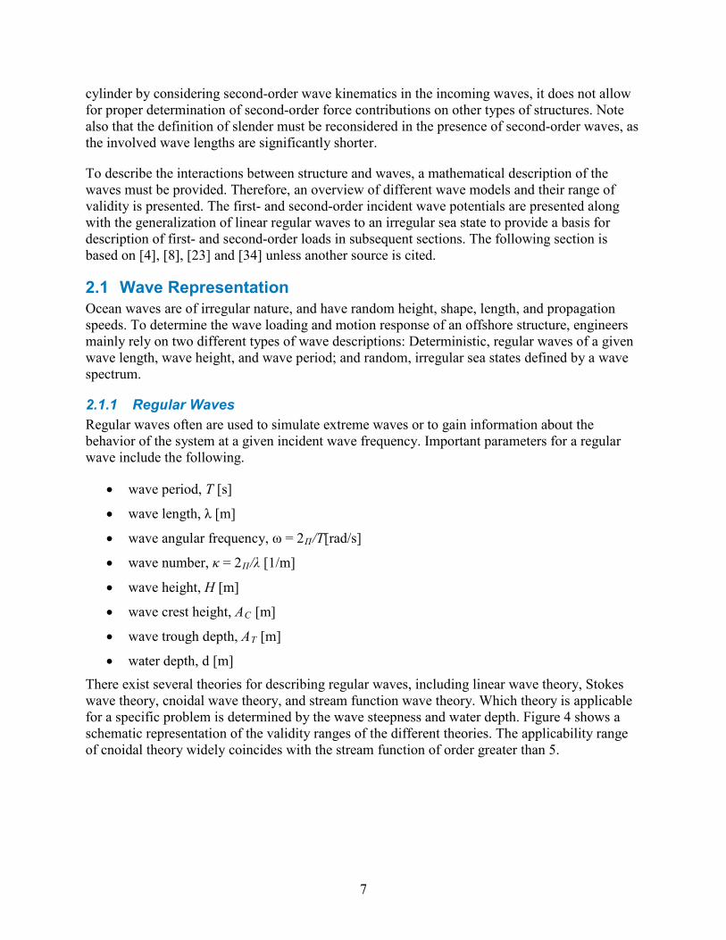
• water depth, d [m] There exist several theories for describing regular waves, including linear wave theory, Stokes wave theory, cnoidal wave theory, and stream function wave theory. Which theory is applicable for a specific problem is determined by the wave steepness and water depth. Figure 4 shows a schematic representation of the validity ranges of the different theories. The applicability range of cnoidal theory widely coincides with the stream function of order greater than 5.
8
Figure 4. Validity ranges of different wave theories; the horizontal axis is a measure of shallowness and the vertical axis a measure of wave steepness [4].
Linear wave theory is the simplest regular wave theory. It can be derived from the first-order hydrodynamic problem for potential flow described above, assuming that there is no body present in the waves. This means that it assumes that the wave amplitudes are small compared to both the wave length and the water depth. It describes the waves as sine waves dependent on time and position, giving the following expression for the wave elevation
ζ(t,x,y) = A sin (ωt+ κ(xcosβ + ysinβ)) , (2-1)
where t is time and (x,y) is the position on the free surface, A is the wave amplitude, ω is the wave angular frequency, and β is the wave heading. The wave number κ depends on the water depth h, the wave frequency ω and the gravitational acceleration g, and is given by
κ = ω2/g for infinite water depth, (2-2)
κtanh (κh) = ω2/g for finite water depth. (2-3)
The velocity potential Φ1 for a sinusoidal wave is known, and is given by Equation 2–4.
𝜙𝐼 =𝑔𝐴𝜔𝑍(𝜅𝑧) sin(𝜔𝑡 + 𝜅(𝑥𝑐𝑜𝑠𝛽 + 𝑦𝑠𝑖𝑛𝛽))
(2-4)
9
The function Z(κz) describes the depth dependence of the potential, and is given by
Z(κz) = eκz for infinite water depth, (2-5)
𝑍(𝜅𝑧) = cosh (𝜅(𝑧+ℎ))cosh (𝜅ℎ)
for finite water depth. (2-6)
An important characteristic of the linear wave is the rapid decay of the velocity potential with water depth—meaning that the influence of the incident waves is limited to the region near the free-surface. This is especially true for shorter waves with a high wave number. For a linear wave, the water particles travel along closed trajectories, and this is why the depth penetration of the potential changes with water depth. In deep water, the water particles travel along circular trajectories. As the water depth decreases, the trajectories become increasingly flatter ellipsoids.
Because the wave is sinusoidal, wave crest height AC is equal to wave trough height AT. They are both equal to the wave amplitude AC = AT = A = H/2. The phase velocity c of the wave is given by
𝑐 = �𝑔𝜅𝑡𝑎𝑛ℎ(𝜅𝑑) for general water depth,
(2-7)
c = gT/(2Π) for deep water. (2-8)
Be aware that the wave length and wave period do not depend explicitly on wave height—which means that a range of different wave heights is possible for a given wave period. The maximum possible wave height for a given wave period is determined by the breaking wave limit, as shown in Figure 4. In the case of steep waves close to the breaking limit, linear wave theory generally is not a good model, and the wave should be modeled using non-linear wave theory. One general characteristic of non-linear regular waves is that they have steeper crests and wider troughs than linear waves, with Ac > AT.
Cnoidal theory is generally valid for shallow water (e.g., wave amplitude is not required to be small compared to water depth), and Stokes theory is applicable for steep waves in deep water. Stream function is a purely numerical theory that has a wider application range. Stokes wave theory builds on the potential flow assumption given above, whereas cnoidal or stream function waves do not require the formulation of a velocity potential. More information and other references for these wave theories can be found in [4].
2.1.2 Irregular Waves Irregular wave theory describes the waves as they are observed on the ocean: random and irregular. A typical assumption is that the surface elevation is part of a statistically stationary process with duration of from 20 minutes to 6 hours. The conditions throughout this period are called “sea state.” A sea state is characterized by a set of parameters, i.e., the significant wave height HS and the peak-spectral period Tp. The significant wave height is defined as the average wave height of the highest one-third of the waves, and is similar to the wave height perceived by humans [30]. The peak period is the period related to the peak of the spectrum, i.e., Tp = 2Π/ωp, where ωp is the wave frequency at the spectrum peak.
10
Irregular waves are modeled as a summation of linear wave components. The simplest model for an irregular sea state is the linear long-crested wave model, where the first-order wave elevation ζ is given by
𝜁(𝑡) = 𝑅𝑒��𝐴𝑗𝑒𝑖𝜔𝑗
𝑁
𝑗=1
� . (2-9)
Here 𝐴𝑗 = 𝑎𝑗𝑒𝑖𝜑𝑗 is the complex wave amplitude belonging to the wave frequency ωj, with magnitude 𝑎𝑗 and random phase 𝜑𝑗. The number of wave components used to describe the sea state is designated N. The random phases are uniformly distributed between 0 and 2Π, and the magnitudes are defined through a wave spectrum S(ω) by the relation
𝑎𝑗2 = 2 𝑆(𝜔𝑗)Δ𝜔𝑗 , (2-10)
where Δωj is the difference between two successive frequencies. If the equal-frequency spacing is used, it is important to be aware that the wave elevation will repeat itself after 2Π/ω s. For long simulations it is practical to use other frequency spacing methods, such as choosing the frequency randomly in the interval (ωj –Δω/2,ωj + Δω/2) [8] or using the equal-energy spacing method [35].
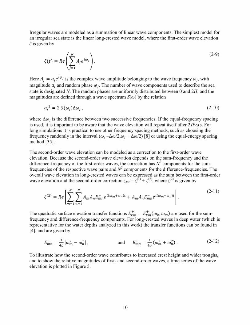
The second-order wave elevation can be modeled as a correction to the first-order wave elevation. Because the second-order wave elevation depends on the sum-frequency and the difference-frequency of the first-order waves, the correction has N2 components for the sum-frequencies of the respective wave pairs and N2 components for the difference-frequencies. The overall wave elevation in long-crested waves can be expressed as the sum between the first-order wave elevation and the second-order correction ζtot = ζ(1) + ζ(2), where ζ(2) is given by
𝜁(2) = 𝑅𝑒 �� �𝐴𝑚𝐴𝑛𝐸𝑚𝑛+ 𝑒𝑖(𝜔𝑚+𝜔𝑛)𝑡 + 𝐴𝑚𝐴𝑛𝐸𝑚𝑛− 𝑒𝑖(𝜔𝑚−𝜔𝑛)𝑡𝑁
𝑛=1
𝑁
𝑚=1
� . (2-11)
The quadratic surface elevation transfer functions 𝐸𝑘𝑚± = 𝐸𝑘𝑚
± (𝜔𝑘,𝜔𝑚) are used for the sum-frequency and difference-frequency components. For long-crested waves in deep water (which is representative for the water depths analyzed in this work) the transfer functions can be found in [4], and are given by
𝐸𝑚𝑛− = 14𝑔
|𝜔𝑚2 − 𝜔𝑛2| , and 𝐸𝑚𝑛+ = 14𝑔
(𝜔𝑚2 + 𝜔𝑛2) . (2-12)
To illustrate how the second-order wave contributes to increased crest height and wider troughs, and to show the relative magnitudes of first- and second-order waves, a time series of the wave elevation is plotted in Figure 5.
11
Figure 5. Wave elevation with and without second-order correction
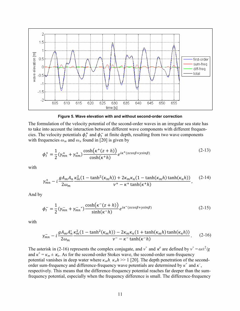
The formulation of the velocity potential of the second-order waves in an irregular sea state has to take into account the interaction between different wave components with different frequen-cies. The velocity potentials 𝜙𝐼+ and 𝜙𝐼− at finite depth, resulting from two wave components with frequencies ωm and ωn found in [20] is given by
𝜙𝐼+ =12
(𝛾𝑚𝑛+ + 𝛾𝑛𝑚+ )cosh�𝜅+(𝑧 + ℎ)�
cosh(𝜅+ℎ) 𝑒𝑖𝜅+(𝑥𝑐𝑜𝑠𝛽+𝑦𝑠𝑖𝑛𝛽) (2-13)
with
𝛾𝑚𝑛+ − 𝑖𝑔𝐴𝑚𝐴𝑛
2𝜔𝑚𝜅𝑚2 (1 − tanh2(𝜅𝑚ℎ)) + 2𝜅𝑚𝜅𝑛(1 − tanh(𝜅𝑚ℎ) tanh(𝜅𝑛ℎ))
𝜈+ − 𝜅+ tanh(𝜅+ℎ) , (2-14)
And by
𝜙𝐼− =12
(𝛾𝑚𝑛− + 𝛾𝑚𝑛− ∗)cosh�𝜅−(𝑧 + ℎ)�
sinh(𝜅−ℎ) 𝑒𝑖𝜅−(𝑥𝑐𝑜𝑠𝛽+𝑦𝑠𝑖𝑛𝛽) (2-15)
with
𝛾𝑚𝑛− − 𝑖𝑔𝐴𝑚𝐴𝑛∗
2𝜔𝑚𝜅𝑚2 (1 − tanh2(𝜅𝑚ℎ)) − 2𝜅𝑚𝜅𝑛(1 + tanh(𝜅𝑚ℎ) tanh(𝜅𝑛ℎ))
𝜈− − 𝜅− tanh(𝜅−ℎ) . (2-16)
The asterisk in (2-16) represents the complex conjugate, and v+ and κ± are defined by v+ = ω±2/g and κ± = κm ± κn. As for the second-order Stokes wave, the second-order sum-frequency potential vanishes in deep water where κmh, κnh >> 1 [20]. The depth penetration of the second-order sum-frequency and difference-frequency wave potentials are determined by κ+ and κ–, respectively. This means that the difference-frequency potential reaches far deeper than the sum-frequency potential, especially when the frequency difference is small. The difference-frequency
12
potential therefore can be expected to have an effect on structural members deeper in the water, such as the pontoons of a semi-submersible platform.
As noted, the formulations for the velocity potentials are derived for long-crested seas, and the analysis in this work is performed for such conditions. Long-crested seas means that the waves comes only from one direction, and essentially can be treated as two dimensional. The equations given above for long-crested seas, however, can easily be extended to include directionality and short-crested waves. Details on how to do this are found in [34] and [4].
2.1.3 Wave Spectrum There are several wave spectra that are commonly used for design of offshore structures depending on the environmental condition at the site. Important parameters are wind fetch, wave types, and water depth.
When the wind starts blowing and waves start forming, it takes some time before equilibrium between the energy added to the waves by the wind and the energy dissipated by the ocean is reached. A sea state in which this balance prevails is called a fully developed sea state. There are several reasons why this equilibrium might not be reached. It might be that the wind only has been blowing for a short time, in which case the sea state is described as a developing sea state. It also could be that the distance across which the waves are allowed to build up is limited; a condition that creates a fetch-limited sea state. Another factor that impacts the frequency content of a wave spectra is the distribution of swell and wind waves. Wind waves are waves created by local wind conditions, as described above. Swells are waves that have travelled from where they were generated into the considered area, and have no relationship to local winds.
The Pierson-Moscowitz spectrum SPM(ω) is a two-parameter spectrum created for fully developed seas. It was created based on wind and wave records from British weather ships positioned in the North Atlantic and was published in 1964, and is given by
𝑆𝑃𝑀(𝜔) =5
16𝐻𝑠2𝜔𝑝4𝜔−5𝑒𝑥𝑝 �−
54�𝜔𝜔𝑝�−4
� . (2-17)
The formulation is based on only two parameters, the significant wave height HS and the peak-spectral frequency ωp = 2Π/Tp.
The JONSWAP spectrum was developed as part of the Joint North Sea Wave Project and published in 1973. The spectrum describes a developing sea in a limited-fetch situation. It is given by
𝑆𝐽(𝜔) = 𝐴𝛾 𝑆𝑃𝑀(𝜔) 𝛾𝑒𝑥𝑝�−12�
𝜔−𝜔𝑝𝜎 𝜔𝑝
�2�
, (2–18)
where Aγ = 1 – 0.287ln(γ) is a normalizing factor and σ is a spectral width parameter with σ = σa for σ ≤ ωp and σ = σb for σ > ωp. Because of the many parameters, the JONSWAP spectrum can be more flexibly fitted to measured site data than the Pierson-Moscowitz spectrum. For this work, the average values for the JONSWAP spectrum given in [4] are used: γ = 3.3, σa = 0.07
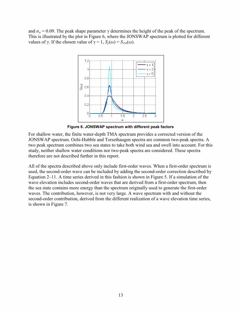
13
and σa = 0.09. The peak shape parameter γ determines the height of the peak of the spectrum. This is illustrated by the plot in Figure 6, where the JONSWAP spectrum is plotted for different values of γ. If the chosen value of γ = 1, Sj(ω) = SPM(ω).
Figure 6. JONSWAP spectrum with different peak factors
For shallow water, the finite water-depth TMA spectrum provides a corrected version of the JONSWAP spectrum. Ochi-Hubble and Torsethaugen spectra are common two-peak spectra. A two peak spectrum combines two sea states to take both wind sea and swell into account. For this study, neither shallow water conditions nor two-peak spectra are considered. These spectra therefore are not described further in this report.
All of the spectra described above only include first-order waves. When a first-order spectrum is used, the second-order wave can be included by adding the second-order correction described by Equation 2–11. A time series derived in this fashion is shown in Figure 5. If a simulation of the wave elevation includes second-order waves that are derived from a first-order spectrum, then the sea state contains more energy than the spectrum originally used to generate the first-order waves. The contribution, however, is not very large. A wave spectrum with and without the second-order contribution, derived from the different realization of a wave elevation time series, is shown in Figure 7.
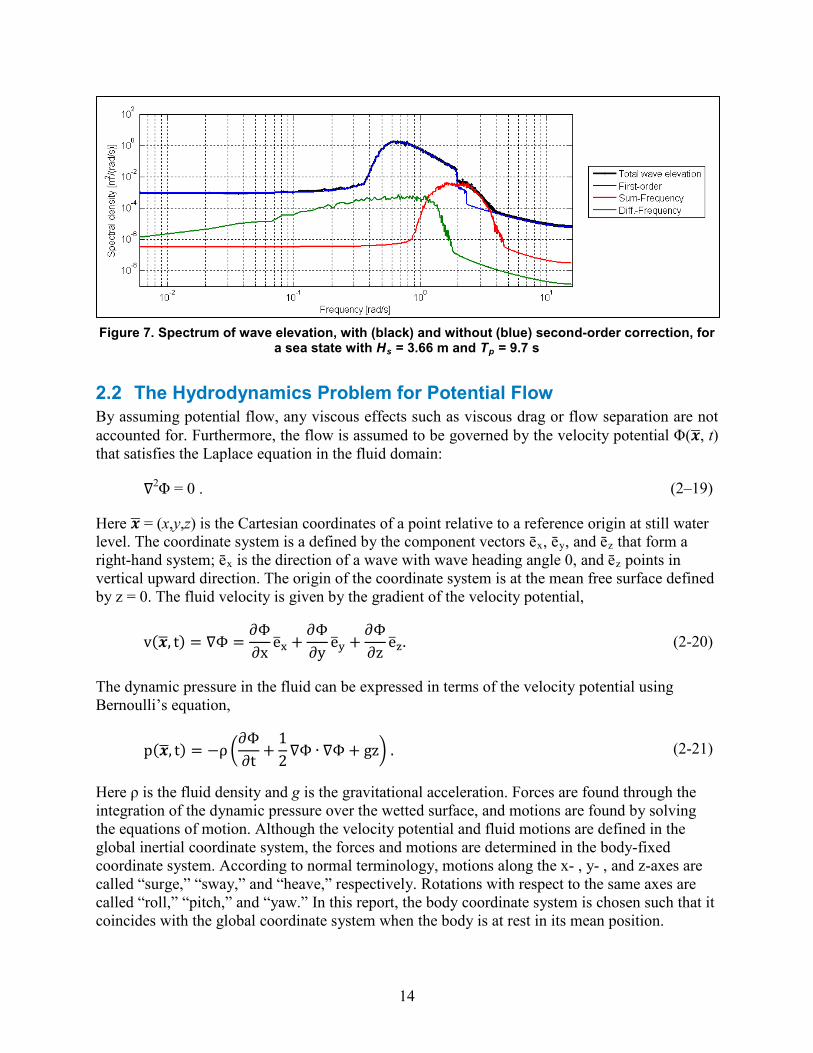
14
Figure 7. Spectrum of wave elevation, with (black) and without (blue) second-order correction, for a sea state with Hs = 3.66 m and Tp = 9.7 s
2.2 The Hydrodynamics Problem for Potential Flow By assuming potential flow, any viscous effects such as viscous drag or flow separation are not accounted for. Furthermore, the flow is assumed to be governed by the velocity potential Φ(𝒙�, t) that satisfies the Laplace equation in the fluid domain:
∇2Φ = 0 . (2–19)
Here 𝒙� = (x,y,z) is the Cartesian coordinates of a point relative to a reference origin at still water level. The coordinate system is a defined by the component vectors ēx, ēy, and ēz that form a right-hand system; ēx is the direction of a wave with wave heading angle 0, and ēz points in vertical upward direction. The origin of the coordinate system is at the mean free surface defined by z = 0. The fluid velocity is given by the gradient of the velocity potential,
v(𝒙�, t) = ∇Φ =∂Φ∂x
e�x +∂Φ∂y
e�y +∂Φ∂z
e�z. (2-20)
The dynamic pressure in the fluid can be expressed in terms of the velocity potential using Bernoulli’s equation,
p(𝒙�, t) = −ρ�∂Φ∂t
+12∇Φ ∙ ∇Φ + gz� . (2-21)
Here ρ is the fluid density and g is the gravitational acceleration. Forces are found through the integration of the dynamic pressure over the wetted surface, and motions are found by solving the equations of motion. Although the velocity potential and fluid motions are defined in the global inertial coordinate system, the forces and motions are determined in the body-fixed coordinate system. According to normal terminology, motions along the x- , y- , and z-axes are called “surge,” “sway,” and “heave,” respectively. Rotations with respect to the same axes are called “roll,” “pitch,” and “yaw.” In this report, the body coordinate system is chosen such that it coincides with the global coordinate system when the body is at rest in its mean position.
15
2.2.1 Boundary Conditions Boundary conditions are imposed on the free surface, on the body surface and on the seabed. At the solid surfaces a no flow condition is imposed. For the sea bed, this implies that the normal velocity at the boundary must be zero, i.e.,
𝑣𝑧 = 𝜕𝛷𝑧𝜕𝑧
= 0 when z = –h, (2-22)
or that the velocity potential converges to zero for infinite water depth,
∇Φ →0 when z →∞ . (2-23)
The impermeability condition requires the relative velocity at the body boundary to be zero:
𝑣𝑛 = 𝜕𝛷𝑛𝜕𝑛�
= 𝑢𝑛 = 𝒖 ∙ 𝒏 at body surface (2-24)
Here, n is the normal vector of the surface and u is the velocity of the structure (which is 0 if the structure is fixed). At the free-surface there are two different boundary conditions. The first is the dynamic boundary condition, which ensures that the pressure on the surface is equal to the air pressure. This is derived from the Bernoulli equation, assuming that the pressure is the same all over the free surface:
− 1𝜌
(𝑝 − 𝑝𝑎) = ∂Φ∂t
+ 12∇Φ ∙ ∇Φ + gz = 0 at the free-surface z = 𝜁. (2-25)
The second condition is the kinematic free-surface boundary condition,which requires a particle on the free-surface to have the same vertical velocity as the free-surface itself. It is is derived by requiring that the substantial derivative of the difference between the free-surface elevation ζ and the instantaneous vertical position of the particle z vanishes, leading to
0 = 𝐷𝐷𝑡
(𝑧 − 𝜁) = 𝜕𝛷𝜕𝑧− 𝜕𝜁
𝜕𝑡− 𝜕𝛷
𝜕𝑥𝜕𝜁𝜕𝑥− 𝜕𝛷
𝜕𝑦𝜕𝜁𝜕𝑦− 𝜕𝛷
𝜕𝑧𝜕𝜁𝜕𝑧
at the free-surface z = 𝜁 . (2-26)
The two free-surface boundary conditions can be combined to give a single condition for the velocity potential,
∂Φ∂t2
+ g∂Φ∂z
+ 2∇Φ ∙ ∇∂Φ∂t
+12∇Φ ∙ ∇(∇Φ ∙ ∇Φ) = 0 ,
(2-27)
which applies on the exact free-surface as given by
𝜁(𝑥,𝑦) = −1𝑔�∂Φ∂t
+12∇Φ ∙ ∇Φ�
𝑧=𝜁 .
(2-28)
The last conditions (2-18) is the radiation condition at infinity. The radiation condition is needed for the solution to be unique because there are no prescribed initial conditions, only a assumption of sinusoidal time dependence at all previous time. The radiation condition states that all waves other than the incident waves are due the presence of the body, and must radiate away from it.
16
Using energy conservation, the waves at infinity must be of the general form given in Equation 2–29 for all potentials except the incident wave potential.
𝛷 ∝ 𝑅−1 2⁄ 𝑒−𝑖𝑘𝑅, as 𝑅 = (𝑥2 + 𝑦2)1 2⁄ → ∞ (2-29)
2.2.2 Assumptions Apart from the assumptions that enable the use of potential flow theory for the description of the problem, there are two requirements that are crucial to the further derivation. First, the wave amplitude is assumed to be small compared to the wave length, i.e., we assume that the wave slope is small. Second, the motion amplitudes also are assumed to be small, in the same order of magnitude as the wave amplitude. With these conditions fulfilled, the following conclusions can be drawn.
• Assuming a small wave, amplitude is consistent with the use of linear wave theory.
• A sufficiently small wave amplitude justifies the expansion of the problem in terms of wave slope.
• With small motion amplitudes and small waves, it is possible to divide the hydrodynamics problem into sub-problems (hydrostatics, radiation, and diffraction) and it is possible to use superposition of different parts of the wave-structure interactions to obtain the overall solution in regular waves.
• The results obtained in regular waves ultimately can be generalized to more representative motions in irregular waves by superposition of sinusoidal components.
For simplicity, the theory is presented for a single structure, ignoring possible interactions with walls or other structures. It also is assumed that all motions are rigid-body motions, and that all waves propagate in the same direction.
2.2.3 Perturbation Series To facilitate the solution of the hydrodynamics problem described above, the velocity potential is expressed as a perturbation series in terms of the incident wave slope as given by
Φ(𝐱�, t) = Φ(1)(𝐱�, t) + Φ(2)(𝐱�, t) + … (2-30)
Here, Φ(1) and Φ(2) are the first- and second-order velocity potentials with respect to the wave amplitude, such that Φ(1) ~ A and Φ(2) ~ A2. The other hydrodynamic quantities also are expanded, leading to first- and second-order expressions for the free-surface elevation, pressure, and motions. The first- and second-order wave elevation is given by
𝜁(1)(𝑥,𝑦) = −1𝑔∂Φ(1)
∂t 𝑧=0 ,
(2-31)
𝜁(2)(𝑥,𝑦) = −1𝑔�∂Φ(2)
∂t+
12∇Φ(1) ∙ ∇Φ(1) −
1g∂Φ(1)
∂t∂2Φ(1)
∂z ∂t�𝑧=0
, (2-32)
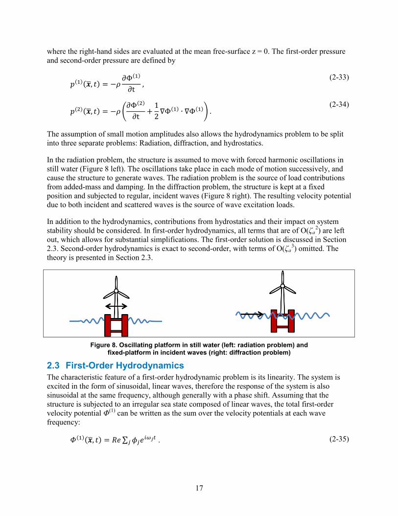
17
where the right-hand sides are evaluated at the mean free-surface z = 0. The first-order pressure and second-order pressure are defined by
𝑝(1)(𝒙�, 𝑡) = −𝜌∂Φ(1)
∂t ,
(2-33)
𝑝(2)(𝒙�, 𝑡) = −𝜌�∂Φ(2)
∂t+
12∇Φ(1) ∙ ∇Φ(1)� .
(2-34)
The assumption of small motion amplitudes also allows the hydrodynamics problem to be split into three separate problems: Radiation, diffraction, and hydrostatics.
In the radiation problem, the structure is assumed to move with forced harmonic oscillations in still water (Figure 8 left). The oscillations take place in each mode of motion successively, and cause the structure to generate waves. The radiation problem is the source of load contributions from added-mass and damping. In the diffraction problem, the structure is kept at a fixed position and subjected to regular, incident waves (Figure 8 right). The resulting velocity potential due to both incident and scattered waves is the source of wave excitation loads.
In addition to the hydrodynamics, contributions from hydrostatics and their impact on system stability should be considered. In first-order hydrodynamics, all terms that are of O(ζa
2) are left out, which allows for substantial simplifications. The first-order solution is discussed in Section 2.3. Second-order hydrodynamics is exact to second-order, with terms of O(ζa
3) omitted. The theory is presented in Section 2.3.
Figure 8. Oscillating platform in still water (left: radiation problem) and fixed-platform in incident waves (right: diffraction problem)
2.3 First-Order Hydrodynamics The characteristic feature of a first-order hydrodynamic problem is its linearity. The system is excited in the form of sinusoidal, linear waves, therefore the response of the system is also sinusoidal at the same frequency, although generally with a phase shift. Assuming that the structure is subjected to an irregular sea state composed of linear waves, the total first-order velocity potential Φ(1) can be written as the sum over the velocity potentials at each wave frequency:
𝛷(1)(𝒙�, 𝑡) = 𝑅𝑒∑ 𝜙𝑗𝑒𝑖𝜔𝑗𝑡𝑗 . (2-35)
18
Here, Φj is the complex velocity potential belonging to the frequency ωj. For simplicity, this section omits the index j that notifies the relation to frequency ωj, with a lowercase Φ referring to the velocity potential belonging to one specific frequency. The velocity potential Φ can be split into the radiation potential ΦR and the diffraction potential ΦD. The diffraction potential can be further decomposed into an incident wave potential Φ1 and a scattered wave potential ΦS as given by
𝜙 = 𝜙𝑅 + 𝜙𝐷 = 𝜙𝑅 + 𝜙𝐼 + 𝜙𝑆 . (2-36)
The total velocity potential and all the separate components satisfy the Laplace equation. Another important simplification in the first-order problem is the linearization of the free-surface boundary condition, which can be expressed as
𝜕𝜙𝜕𝑧− 𝜔2
𝑔𝜙 = 0 on z = 0 . (2-37)
2.3.1 Radiation Problem A structure that moves around in fluid experiences force contributions from added-mass and damping. When a free surface is present, the motion also causes wave generation. This wave radiation leads to a memory effect and an outgoing energy flux that damps the motion. The force in direction i due to a sinusoidal motion of unit amplitude in direction j is given by the force coefficient 𝑓𝑖𝑗(𝜔), computed as
𝑓𝑖𝑗(𝜔) = −𝜌∬ 𝜕𝜙𝑖𝜕𝑛𝜙𝑗𝑑𝑆𝑆𝐵
, 𝑖, 𝑗 = 1, 2, … , 6 . (2-38)
The potentials Φi and Φj are the radiation potentials connected to the forced oscillation of frequency 𝜔 in direction i and j, respectively. They are found by solving the boundary value problem described above, with the boundary condition at the wetted body surface SB being
𝜕𝜙𝑗𝜕𝑛
= 𝑖𝜔𝑛𝑗 , j = 1, 2, 3 (2-39)
𝜕𝜙𝑗𝜕𝑛
= 𝑖𝜔(𝒓 × 𝒏)𝑗−3 , j = 4, 5, 6 (2-40)
where n is the surface normal vector and r is the position vector (x, y, z). The force coefficients take the form
𝑓𝑖𝑗(𝜔) = 𝜔2𝐴𝑖𝑗(𝜔) − 𝑖𝜔𝐵𝑖𝑗(𝜔) (2–41)
with Aij being the contribution from added mass and Bij the damping contribution from wave radiation damping. The total force can be written as
𝐹𝑖(𝜔) = 𝑅𝑒 �∑ 𝜉𝑗𝑒𝑖𝜔𝑡𝑓𝑖𝑗6𝑗=1 (𝜔)� , for 𝑖, 𝑗 = 1, … , 6
= −∑ �𝐴𝑖𝑗(𝜔)�̇�𝑗 + 𝐵𝑖𝑗(𝜔)𝑈𝑗�6𝑗=1 , for 𝑖, 𝑗 = 1, … , 6
(2–42)
19
From the last formulation, it is clear that the added mass Aij adds to the system inertia term as it is multiplied with the body acceleration. The damping contribution also is recognized easily as a term proportional to the velocity. Because the coefficients are real, they are in phase with the motions. Both Aij and Bij are symmetric, such that fij = fji. The damping coefficients Bij are 0 at the infinite and zero frequency limits, whereas the added-mass coefficients Aij have non-zero limits.
2.3.2 Diffraction Problem The wave-excitation forces created by an incident wave of frequency ω can be found from the integral of the pressure over the wetted surface SB. Written in terms of the velocity potentials, the force coefficient Xi is given by
𝑋𝑖 = −𝜌∬ (𝜙𝐼 + 𝜙𝑆) 𝜕𝜙𝑖𝜕𝑛
𝑑𝑆𝑆𝐵 , i = 1, 2, …, 6 . (2–43)
The force coefficient Xi which describes the force in direction i for a regular wave of unit amplitude and frequency ω. The potentials Φi are the radiation potentials of Equation 2–39 and Equation 2–40. As long as only terms of first-order are of interest, this integral can be evaluated at the mean position of the body. This means that the first-order wave excitation forces are independent of whether the structure is freely floating, moored, or fixed, and that the distinctions between these arrangements are of second-order or higher.
The velocity potential of the first-order incident wave Φi is given by Equation (2-4). Because the incident wave potential already is known and the diffraction problem is solved assuming that the structure is at its mean position, the boundary condition for the scattering potential ΦS at the body boundary can be rewritten in terms of the incident wave potential:
𝜕𝜙𝑆𝜕𝑛
= −𝜕𝜙𝐼𝜕𝑛
. (2-44)
With this boundary condition and some mathematics, the integral of Equation 2–43 can even be rearranged to be independent of the scattering potential. To obtain the force from a “real” wave, the force coefficient must be multiplied with the complex amplitude of the incident wave A. The proper expression for the wave excitation load 𝐹𝑒𝑥𝑖 in time domain is then
𝐹𝑒𝑥𝑖 = 𝑅𝑒�𝐴𝑋𝑖𝑒𝑖𝜔𝑡� , i = 1, 2, …, 6 (2-45)
For an irregular sea state, the wave excitation forces 𝐹𝑒𝑥(1) are calculated through superposition
of the forces from all 𝑛𝑊 wave components.
𝐹𝑒𝑥𝑖 = 𝑅𝑒�∑ 𝐴𝑗𝑋𝑖,𝑗𝑒𝑖𝜔𝑗𝑡𝑗 � , i = 1, 2, …, 6 and j =1, …, 𝑛𝑤 (2-46)
2.3.3 Hydrostatics The hydrostatic forces and moments keep a structure floating and in a stable position. Buoyancy forces, gravity restoring terms and changes in the submerged portion of the structure all contribute to the hydrostatic stability. The complete hydrostatic force can be found from the integral of the static pressure over the wetted surface of the body. It is given by
20
𝐹𝑖 = (𝜌𝑉0 − 𝑚)𝑔𝛿𝑖3 − (𝑚𝑦𝐺 − 𝜌𝑉0𝑦𝐵)𝑔𝛿𝑖4 + (𝑚𝑥𝐺 − 𝜌𝑉0𝑥𝐵)𝑔𝛿𝑖5 −�𝑐𝑖𝑗𝜉𝑗
6
𝑗=1
, (2-47)
with i = 1, 2, …, 6. The first three terms are the contributions from the gravity and buoyancy needed to keep the platform in its mean position. The terms (𝑥𝐺 , 𝑦𝐺 , 𝑧𝐺) and (𝑥𝐵, 𝑦𝐵 , 𝑧𝐵) are the position of the center of gravity (CoG) and center of buoyancy (CoB) when the turbine is in the mean position, and V0 is the displaced volume (for a freely floating body pV0 = m, the mass of displaced water equals the mass of the body). The cij in the last term is the components of the hydrostatic stiffness matrix that induce a force or moment as soon as the structure moves and the displacements 𝜉𝑗 are no longer 0.
𝐶 =
⎣⎢⎢⎢⎢⎢⎢⎢⎢⎢⎢⎢⎡ 0 0 0
0 0 00 0 𝜌𝑔𝐴0
0 0 00 0 0
𝜌𝑔�𝑦𝐴0
𝑑𝐴0 −𝜌𝑔�𝑥𝐴0
𝑑𝐴0 0
0 0 𝜌𝑔�𝑦𝐴0
𝑑𝐴0
0 0 −𝜌𝑔�𝑥𝐴0
𝑑𝐴0
0 0 0
𝜌𝑔�𝑦2
𝐴0
𝑑𝐴0 + 𝜌𝑔𝑉0𝑧𝐵 − 𝑚𝑔𝑧𝐺 0 −𝜌𝑔𝑉0𝑥𝐵 + 𝑚𝑔𝑥𝐺
0 𝜌𝑔�𝑥2
𝐴0
𝑑𝐴0 + 𝜌𝑔𝑉0𝑧𝐵 − 𝑚𝑔𝑧𝐺 −𝜌𝑔𝑉0𝑦𝐵 + 𝑚𝑔𝑦𝐺
0 0 0 ⎦⎥⎥⎥⎥⎥⎥⎥⎥⎥⎥⎥⎤
(2-48)
Here A0 is the waterplane area of the undisplaced structure, and the waterplane moments in 𝑥 direction are ∬ 𝑥𝐴0
𝑑𝐴0 and ∬ 𝑥2𝐴0𝑑𝐴0.
This matrix can be simplified for most cases. If the CoG and CoB lie on the centerline of the structure, then there is no coupling from yaw to pitch and roll, and the matrix is symmetric (i.e., (4,6) and (5,6) are 0). Further, if the xz-plane is a symmetry plane, then the (3,4) and (4,3) components are 0. If the yz-plane is also a symmetry plane, the only non-zero components are (3,3), (4,4), and (5,5), and there is no coupling between the modes.
The restoring terms in the hydrostatic stiffness matrix can be divided into three groups:
1. Hydrostatic restoring due to the waterplane moments (all terms that include a surface integral over A0),
2. Hydrostatic restoring due to buoyancy force (all terms that include either xB, yB, or zB), 3. Gravity restoring (all terms that include either xG, yG, or zG).
It is important to be aware that hydrostatics only provides restoring for heave, roll, and pitch. The other modes must be restored by the mooring system. For the body to be statically stable, the coefficients in C have to oppose small displacements ξj. The necessary condition in heave, roll, and pitch is that the corresponding diagonal term is positive. For heave, this always is the case if the waterline area is not 0. For roll and pitch it is a necessary and sufficient condition that the metacentric heights are positive, which is the case when the metacenters zY and zX (given by Equation 2-36) lie above zG.
21
𝑧𝑦 = �∬ 𝑦2𝐴0𝑑𝐴0� 𝑉0� + 𝑧𝐵 and 𝑧𝑥 = �∬ 𝑥2𝐴0
𝑑𝐴0� 𝑉0� + 𝑧𝐵 (2-36)
For a surface-piercing structure, the metacenter always is above the center of buoyancy due to the contribution from the waterplane area, A0. This approach, in which the linear coefficients are used to account for the hydrostatics, is possible only when the motions are relatively small. If the motions are significant enough to cause abrupt changes in water plane area, a different approach in which the instantaneous coefficients of C are calculated must be considered. This, however, is not the case for any of the analyses considered here.
2.3.4 Equations of Motion The coefficients for hydrodynamic excitation forces, added mass, damping, and hydrostatic restoring from the frequency domain can be used to solve the equations of motion. This can be done either in frequency or time domain. The two different methods are based on different assumptions, which make them suitable for different purposes; both are presented below.
When solving the equations in time domain, results from the frequency domain are used to derive time-domain coefficients. For a structure subjected to regular incident waves, which by definition propagate in one direction with a single frequency and amplitude, the equation of motion is given by
(𝑀 + 𝐴(𝜔))�̈� + (𝐵(𝜔) + 𝐵𝑒𝑥𝑡)�̇� + �𝐶ℎ𝑦𝑑𝑟𝑜 + 𝐶𝑒𝑥𝑡�𝑞 = 𝐹𝑒𝑥(1)(𝜔) , (2-49)
where 𝑞 is the instantaneous position of the platform, and is assumed to be a sinusoidal motion 𝑞 = 𝑞� sin(𝜔𝑡). Further, �̇� denotes the velocity and �̈� is the acceleration. M is the mass matrix, A and B are the hydrodynamic added-mass and potential damping at the given frequency, and Chydro is the (frequency-independent) hydrostatic restoring matrix from Equation 2–48. Fex
(1) (ω) is the first-order wave excitation force at the frequency of the incident waves is Fex
(1)(ω). Bext and Cext are external damping and stiffness of the system. In this case, external means any sources of damping or stiffness that is not due to hydrodynamics. Two sources of external damping or stiffness for a wind turbine are the mooring system and the rotor aerodynamics.
When considering irregular waves, the assumption of a single, regular incident wave is no longer correct and Equation 2–49 is not applicable, because the frequency-domain coefficients are no longer directly applicable. They can be used, however, to derive the time-domain coefficients. In this case, the governing equation that must be solved becomes Equation 2–50.
(𝑀 + 𝐴)�̈� + � 𝐾(𝑡 − 𝜏)�̇�(𝜏)𝑑𝜏𝑡
0+ 𝐵𝑒𝑥𝑡�̇� + (𝐶ℎ𝑦𝑑𝑟𝑜 + 𝐶𝑒𝑥𝑡)𝑞 = 𝐹𝑒𝑥(1) (2-50)
M, Bext, Cext, and Chydro are frequency independent and are the same as in Equation 2–49. The wave excitation forces Fex
(1) are calculated through superposition of the forces from all wave components at each time step, as given in Equation 2–46.
The term ∫ 𝐾(𝑡 − 𝜏)�̇�(𝜏)𝑑𝜏𝑡0 is related to the radiation problem, and requires some special
considerations. Only a brief overview is provided here, however; a more thorough explanation can be found in [15], p. 27. Because the body generates waves there is a memory effect related to
22
the free-surface, and all wave radiation loads depend on the motion history of the platform. To use superposition in the radiation problem means that motions are viewed as responses to a succession of individual impulses occurring very close together in time. They all must be taken into account and considered with an appropriate time lag. This is done using a convolution integral in which the function K is called the radiation-retardation kernel, ∫ 𝐾(𝑡 − 𝜏)�̇�(𝜏)𝑑𝜏𝑡
0 .
The equation ∫ 𝐾(𝑡 − 𝜏)�̇�(𝜏)𝑑𝜏𝑡0 accounts for contributions from both added-mass and damping.
The total contribution from the radiation problem can only be found by considering both terms arising from the radiation problem, ∫ 𝐾(𝑡 − 𝜏)�̇�(𝜏)𝑑𝜏𝑡
0 and 𝐴�̈�. Because the two terms are interrelated the formulations for the added mass term and the damping term have to be chosen with regard to each other, and different formulations exist. Another way of expressing the memory effect of the free-surface would for example be by using the acceleration formulation with the convolution kernel L. The two formulations are related to each other as shown in Equation 2–51.
� 𝐾(𝑡 − 𝜏)�̇�(𝜏)𝑑𝜏𝑡
0= � 𝐿(𝑡 − 𝜏)�̈�(𝜏)𝑑𝜏
𝑡
0
(2-51)
Although there are different ways of accounting for the added-mass and damping, what’s important is that all contributions are taken into account without any duplication. Some methods are more common than others, such as that used in HydroDyn [15]. In this case, the added-mass used in the time-domain equation is simply the infinite-frequency limit of the added-mass (Equation 2–52).
𝐴 = lim𝜔→∞
𝐴(𝜔) = 𝐴(∞) (2-52)
In this case, the radiation-retardation kernel K can be found from either the frequency-domain added-mass (Equation 2–53) or from the frequency-domain potential damping (Equation 2–54).
𝐾𝑖𝑗(𝑡) = −2𝜋� 𝜔�𝐴𝑖𝑗(𝜔) − 𝐴𝑖𝑗(∞)� sin(𝜔𝑡)𝑑𝜔∞
0 (2-53)
𝐾𝑖𝑗(𝑡) =2𝜋� 𝐵𝑖𝑗(𝜔) cos(𝜔𝑡)𝑑𝜔∞
0 (2-54)
Equation (2-54) is more commonly used, as it is easier to handle numerically [15]. When all the coefficients are derived using Equation 2–51 through Equation 2–54, Equation 2–50 can be solved.
The other method for deriving time-series from frequency-domain results is to solve the equations of motion directly in frequency domain. This requires the additional assumption of periodic steady-state motions. The first-order equation of motion for a regular incident wave of frequency ω [41] is shown in Equation 2–55.
23
��−𝜔2 �𝑀𝑖𝑗 + 𝐴𝑖𝑗(𝜔)�+ 𝑖𝜔�𝐵𝑖𝑗(𝜔) + 𝐵𝑒𝑥𝑡,𝑖𝑗� + 𝐶𝑖𝑗 + 𝐶𝑒𝑥𝑡,𝑖𝑗�6
𝑗=1
𝑥𝑗 = 𝑎𝑋𝑖(𝜔) (2-55)
Here, 𝑥𝑗 is the amplitude of the motion, a is the amplitude of the incident wave, and 𝑋𝑖 is the force coefficient. The rest of the coefficients are the same as those used in Equation 2–49. This equation results in a complex amplitude of motion called a linear transfer function (LTF) or a response amplitude operator (RAO), as shown in Equation 2–56.
𝜉𝑗 =𝑥𝑗𝑎
= �𝑋𝑖
�−𝜔2�𝑀𝑖𝑗 + 𝐴𝑖𝑗� + 𝑖𝜔�𝐵𝑖𝑗 + 𝐵𝑒𝑥𝑡,𝑖𝑗� + 𝐶𝑖𝑗 + 𝐶𝑒𝑥𝑡,𝑖𝑗�
6
𝑗=1
(2–56)
The magnitude of ξj is the motion amplitude per incident wave amplitude. The phase of ξj describes the phase shift between the motion and the wave elevation. The time series of motion can be derived by taking the real value of a multiplication between the instantaneous wave elevation and the RAO. For an irregular sea state, the time series of motion is found by summing over all wave frequencies at each time step, similar to the approach to find wave forces.
𝑞𝑗(𝑡) = 𝑅𝑒��𝐴𝑗𝜉𝑗𝑒𝑖𝜔𝑗𝑡𝑁
𝑗=1
� (2-57)
As noted above, only periodic steady-state solutions can be computed in the frequency domain. Transients and external force cannot be accounted for, with the result that all motions have the same frequency as the incident waves. When the equations are solved in the time domain, other sources of loading (such as aerodynamics on the rotor) can be included by adding an additional force to the left-hand side of Equation 2–50. Due to the many sources of coupled dynamics and importance of transient behavior, solving the equations in time domain is more precise for a wind turbine.
2.4 Second-Order Hydrodynamics In the second-order hydrodynamic problem, interactions between two harmonically oscillating components—such as two incident linear waves or a wave and the body oscillating at a first-order frequency—are considered. The result is forces and motions at the sum-frequency and difference-frequency of the incident waves. The velocity potential also has a sum-frequency and a difference-frequency part. The total second-order potential takes the form
𝛷(2)(𝒙�, 𝑡) = 𝑅𝑒��𝜙𝑘𝑙+𝑒𝑖(𝜔𝑘+𝜔𝑙)𝑡 + 𝜙𝑘𝑙
−𝑒𝑖(𝜔𝑘−𝜔𝑙)𝑡
𝑙𝑘
, (2-58)
where, Φkl+ and Φkl
- are the velocity potentials at the sum frequencies ωk + ωl and difference frequencies ωk – ωl. The potentials (and the other second-order quantities) fulfill the symmetry relations given by
24
𝜙𝑘𝑙+ = 𝜙𝑙𝑘
+ and 𝜙𝑘𝑙− = 𝜙𝑙𝑘
−∗, (2-59)
where ωk ≥ ωl ≥ 0. Using a similar decomposition as for the first-order problem, the second-order potential can be split into an incident ΦI
(2), a scattering ΦS(2), and a radiation ΦR
(2) potential. At second order, this decomposition generally is not unique, but has the significant advantage that it leaves all complicated second-order effects to the diffraction problem with velocity potential ΦD
(2) = ΦI(2) + ΦS
(2). Therefore, the radiation problem does not have to be solved specifically for the second-order solution. The radiation coefficients are the same as for the first-order solution, they just must be measured for an oscillating motion at the respective sum-frequency or difference-frequency. Hydrostatics also only depends on the motion of the body, and if the second-order motion is included when the equations of motions are solved then the second-order hydrostatic contribution is taken into account.
The diffraction problem is the only part of the hydrodynamics problem that must be solved specifically at second order. It accounts for second-order potential and all quadratic contributions from first-order terms on the body and the free-surface, and is consistent with the definition of the first-order diffraction problem in the sense that it provides the total second-order wave excitation forces and moments (also called “second-order forces”). The second-order forces 𝐹𝑒𝑥
(2) from the diffraction problem can be split into a contribution due to the second-order potential Fp and a contribution due to the first-order quadratic interactions Fq such that 𝐹𝑒𝑥
(2) is given by
𝐹𝑒𝑥(2) = 𝐹𝑝 + 𝐹𝑞 (2-60)
The main difficulty of the second-order problem is related to the solution of the second-order potential, which must fulfill inhomogeneous free-surface and body boundary conditions. The incident wave potential, which is independent of the structure and its motions, can be derived using the first-order incident potential and is given by Equation 2–13 and Equation 2–15. The only potential that must be solved is the scattering potential. The boundary-value problem for the scattering potential at the sum-frequency and difference-frequency of two bichromatic waves can be expressed as
𝛻2𝜙𝑆± = 0 in the entire fluid domain , (2-61)
𝜕𝜙𝑆±
𝜕𝑧= 0 at the sea bed z = -h , (2-62)
−𝜔±2 + 𝑔 𝜕𝜙𝑆±
𝜕𝑧= 𝑄± on the free-surface z = 0 , (2-63)
𝜕𝜙𝑆±
𝜕𝑛= −𝜕𝜙𝐼
±
𝜕𝑛+ 𝐵± on the body surface , (2-64)
and an additional radiation condition at infinity. The free-surface forcing functions 𝑄± are given by
𝑄+ = 12(𝑞𝑚𝑛+ + 𝑞𝑛𝑚+ ) and 𝑄− = 1
2(𝑞𝑚𝑛− + 𝑞𝑛𝑚− ∗) . (2-65)
25
with
𝑞𝑚𝑛+ = −𝑖𝜔𝑛2𝑔
𝜙𝑛(1) �−𝜔𝑚2
𝜕𝜙𝑚(1)
𝜕𝑧+ 𝑔
𝜕2𝜙𝑚(1)
𝜕𝑧2� + 𝑖𝜔𝑛∇𝜙𝑚
(1)∇𝜙𝑛(1) − 𝑞𝐼𝐼𝑚𝑛+ (2-66)
𝑞𝑚𝑛− = 𝑖𝜔𝑛2𝑔
𝜙𝑛(1)∗ �−𝜔𝑚2
𝜕𝜙𝑚(1)
𝜕𝑧+ 𝑔
𝜕2𝜙𝑚(1)
𝜕𝑧2� − 𝑖𝜔𝑛∇𝜙𝑚
(1)∇𝜙𝑛(1)∗ − 𝑞𝐼𝐼𝑚𝑛− (2-67)
Here, 𝑞𝐼𝐼𝑚𝑛+ and 𝑞𝐼𝐼𝑚𝑛− are the forcing functions for the incident wave problem in absence of the structure. The formulation for the forcing functions B± at the body boundary depends on the first-order motions. They can be derived from the body boundary forcing function given by
𝐵 ≡ 𝒏 ∙ �𝜕𝑯𝜕𝑡 𝒓� − 𝒏 ∙ ��𝜩(1) + 𝜶(1) × 𝒓� ∙ ∇�∇𝛷(1) + �𝜶(1) × 𝒏� ∙ �𝑉(1) − ∇𝛷(1)� . (2-68)
Here, Ξ(1) represents the first-order translational motions, α(1) represents the first-order rotational motions and V(1) ≡ ∂/∂t (Ξ(1) + α(1) × r). H is a matrix with second-order elements that are quadratic products of first-order rotational motions, and is given by
𝑯 = −12��𝛼𝑦2 + 𝛼𝑧2� 0 0−2𝛼𝑥𝛼𝑦 (𝛼𝑥2 + 𝛼𝑧2) 0−2𝛼𝑥𝛼𝑧 −2𝛼𝑦𝛼𝑧 �𝛼𝑥2 + 𝛼𝑦2�
� . (2-69)
When the scattering potential is known, the second-order force contribution due to the second-order potential can be calculated using Equation 2–70.
𝐹𝑝 = −𝜌�𝜕�𝜙𝐼(2) + 𝜙𝑆(2)�
𝜕𝑡𝑆𝐵𝒏𝑑𝑆 (2-70)
The other part of the second-order force—which is due to the quadratic interactions between first-order quantities—does not depend on the second-order potential. The total second-order quadratic force contribution is made up of terms that depend on only the first-order potential, that is, the second-order term from the Bernoulli equation, −1
2𝜌∇𝛷(1) ∙ ∇𝛷(1), and terms that depend
on both the first-order potential and the first-order motions. The total quadratic-force component is given by
𝐹𝑞 = 12𝜌𝑔𝜌 ∫ �𝜁𝑟
(1)�2�1 − 𝑛𝑧2𝒏𝑑𝑙𝑤𝑙 − 𝜌∬ �12∇𝛷
(1) ∙ ∇𝛷(1) + �𝜩(1) + 𝜶(1) × 𝒙�∙ 𝜕𝜕𝑡∇𝛷(1)�𝑆𝐵
𝒏𝑑𝑆
+𝜶(1) × 𝐹(1) − 𝜌𝑔𝐴0 �𝛼𝑥(1)𝛼𝑧
(1)𝑥𝐵 + 𝛼𝑦(1)𝛼𝑧
(1)𝑦𝐵� 𝜅 ,
(2-71)
where 𝜁𝑟(1) = 𝜁(1) − �𝛯𝑧
(1) + 𝛼𝑥(1)𝑦 − 𝛼𝑦
(1)𝑥� is the relative first-order wave height, nz is the z component of the normal vector at z = 0 (and nz = 0 for wall-sided bodies).
26
The expressions for the second-order moments Mp and Mq that correspond to Equation 2–70 and Equation 2–71 can be found in [23]. Note that the free-surface (Q) and body surface (B) forcing functions that appear on the left-hand sides of the boundary conditions for the scattering potential require knowledge about the first-order motions, which are calculated using the frequency-domain version of the first-order equations of motions (Equation 2–56).
The second-order wave excitation forces typically are given as quadratic transfer functions for forces (force QTFs), with a force coefficient Xmk± for each pair of incident waves Am and Ak with frequencies ωm and ωk. The force coefficient is calculated assuming that both incident waves are of unit amplitude. To obtain the force in a real sea state, the coefficients must be multiplied by the complex amplitude of both incident waves. The force time series can be calculated through the sum over all incident wave pairs, given by
𝐹𝑒𝑥(2)(𝑡) = 𝑅𝑒 �� �𝐴𝑚𝐴𝑘𝑋𝑚𝑘+𝑒𝑖(𝜔𝑚+𝜔𝑘)𝑡 + 𝐴𝑚𝐴𝑘∗𝑋𝑚𝑘−𝑒𝑖(𝜔𝑚−𝜔𝑘)𝑡
𝑁
𝑘=1
𝑁
𝑚=1
� . (2-72)
As mentioned, the hydrodynamic forces can be split into contributions from the first-order and second-order potential, typically indexed as q (for quadratic first-order contributions) and p (for second-order potential).
𝑋𝑚𝑘± = 𝑋𝑞,𝑚𝑘± + 𝑋𝑝,𝑚𝑘
± (2-73)
As the computational effort needed to solve the second-order potential is substantial, there have been several attempts to find an approximate solution using only the quadratic term. (Another reason for approximate methods is that there existed no comprehensive solution of the second-order problem until the late 1980s.) Both model tests and numerical simulations have shown that this generally is not a good approximation [19]. In some situations, the quadratic term, however, does dominate the potential term, e.g., for difference-frequency forces where the frequency difference is low. The mean-drift force—which is a special case of the difference-frequency problem with ωm = ωk—is even independent of the second-order potential, and can be derived from the first-order potential alone.
Another, more commonly used attempt to reduce computational time was proposed by [34]. If the wave excitation can be assumed to be narrow banded, only terms where ωm ≈ ωk have an influence, and the solution can be restricted to these frequencies.
The second-order forces are calculated as a correction to the first-order forces, similar to the correction for the wave elevation in Equation 2–11. In the frequency domain, the solution is given as quadratic transfer functions for motions (motion QTFs), and the time series of the second-order motions can be calulated from
𝑞(2)(𝑡) = 𝑅𝑒 �� �𝐴𝑚𝐴𝑘𝜉𝑚𝑘+𝑒𝑖(𝜔𝑚+𝜔𝑘)𝑡 + 𝐴𝑚𝐴𝑘∗𝜉𝑚𝑘
−𝑒𝑖(𝜔𝑚−𝜔𝑘)𝑡𝑁
𝑘=1
𝑁
𝑚=1
� . (2-74)
27
Here, ξmk+ and ξmk– are the motion QTFs for the sum-frequency and difference-frequency
components. The time-domain equation is similar to the first-order time-domain equation of motion Equation 2–50, but with the second-order wave excitation force on the right-hand side.
(𝑀 + 𝐴)�̈�(2) + � 𝐾(𝑡 − 𝜏)�̇�(2)(𝜏)𝑑𝜏𝑡
0+ 𝐵𝑒𝑥𝑡�̇�(2) + (𝐶ℎ𝑦𝑑𝑟𝑜 + 𝐶𝑒𝑥𝑡)𝑞(2) = 𝐹𝑒𝑥(2) (2–75)
To calculate the total motions, the first-order and second-order motions can be superimposed linearly. Alternatively, the time-domain equation of motion can be solved to get the total motions directly by including the first-order wave excitation forces on the right-hand side.
(𝑀 + 𝐴)�̈�𝑡𝑜𝑡 + � 𝐾(𝑡 − 𝜏)�̇�𝑡𝑜𝑡(𝜏)𝑑𝜏𝑡
0+ 𝐵𝑒𝑥𝑡�̇�𝑡𝑜𝑡 + (𝐶ℎ𝑦𝑑𝑟𝑜 + 𝐶𝑒𝑥𝑡)𝑞𝑡𝑜𝑡 = 𝐹𝑒𝑥(1) + 𝐹𝑒𝑥(2)
(2-76)
2.5 Limitations to the Potential Flow Formulation of the Hydrodynamics Problem
The potential flow formulation presented above only partly describes the overall physics of the hydrodynamics problem. The assumptions inherent to the formulation and how they apply to a floating wind turbine have to be assessed. The implications of the different assumptions are discussed in more detail in this section.
2.5.1 Potential Flow Assumption The single most important assumption for the formulation is the assumption of potential flow, which is necessary for the definition of a velocity potential. Potential flow theory means that the flow is irrotational and free of viscous effects, i.e., that there is no flow separation, no vortex shedding, and no influence of viscous drag. The three most important parameters to determine the flow regime and to assess whether the potential flow assumption applies to a specific problem are the Keulegan-Carpenter number, the oscillatory Reynolds number, and the diameter to wavelength ratio [14]. The Keulegan-Carpenter number is a dimensionless number that determines the relative importance of drag force to inertia forces, and is given by
𝐾 =𝑉𝑇𝐷
. (2-77)
Here, T is the wave period, V is the fluid velocity amplitude normal to the cylinder and D is the diameter or characteristic length scale of the structure. The velocity V is given by
𝑉 =𝜋𝐻𝑇
cosh (𝜅(𝑧 + ℎ))sinh(𝜅ℎ)
. (2-78)
The wave number 𝜅 is calculated from the dispersion relation Equation 2–2 and Equation 2–3, h is the water depth and z the depth at which the velocity is calculated. Because the product 𝑉𝑇 is dependent mainly on the wave height H, the Keulegan-Carpenter number basically is a depth-dependent (more accurate) version of the wave height to diameter ratio used for flow regime determination in Figure 3. A Keulegan-Carpenter number greater than 2 generally indicates flow
28
separation. The oscillatory Reynolds number describes the ratio between inertia and viscous forces, and is given by
𝑅𝑒 =𝑉𝐷𝜐
, (2-79)
where 𝜐 is the viscosity of the fluid. The diameter to wavelength ratio D/λ determines the relative slenderness of the structure. If this parameter is less than 0.2, then the scattering of incident waves can be assumed to be unimportant, and the theory that assumes a slender structure can be used.
2.5.2 Wave Modeling Because of the need to simplify the free surface boundary condition, first-order and second-order hydrodynamics based on potential flow assume that the waves are linear (first order) or weakly non-linear (second order). In this work, no higher-order waves are considered, such as third-order or higher-order Stokes waves or wave models derived using stream-function theory.
2.5.3 Viscous Drag Viscous drag and any other viscous effects are ignored in this work. Morison’s equation is a widely used approach to determine forces from viscous drag, if needed. As mentioned in the introduction to this section, the forces are determined directly from incident wave kinematics such that the method does not require the definition of a velocity potential. This more direct representation of the waves also allows for introduction of non-linear wave kinematics and current. The force on a cylinder per length is given by
𝑑𝐹 = 𝜌(1 + 𝐶𝑎)𝜋4𝐷2�̇� +
12𝜌𝐶𝑑𝐷𝑢|𝑢| .
(2-80)
The first term is the inertia force and the second term is the force from viscous drag, with Ca and Cd being the added mass and drag coefficients, D the cylinder diameter, and u and �̇� the velocity and acceleration, respectively. If the radiation-diffraction solution is used to calculate the mass force, then the first term should be omitted. Although Morison’s equation ignores any coupling terms in the added mass matrix, the first term is a reasonably accurate approximation of inertial loading for a slender structure. The drag term commonly is used in conjunction with the radiation-diffraction solution to include viscous drag for slender members. The main problem lies within the determination of Cd which is dependent on many different flow parameters. Some typical values are however found in literature, and over decades successfully have been applied to hydrodynamic problems.
2.5.4 Vortex-Induced Vibrations Vortex shedding is known to cause vortex-induced vibrations of floating platforms, especially for relatively slender structures such as a spar or TLP tendons. The vortex-shedding frequency, fv, is determined by the Strouhal number S, the cross-flow velocity U, and the structure diameter D and is given by
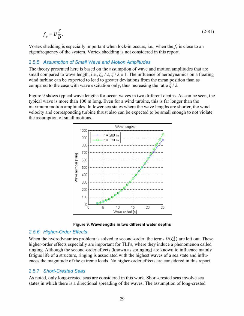
29
𝑓𝑣 = 𝑈𝑆𝐷 . (2-81)
Vortex shedding is especially important when lock-in occurs, i.e., when the fv is close to an eigenfrequency of the system. Vortex shedding is not considered in this report.
2.5.5 Assumption of Small Wave and Motion Amplitudes The theory presented here is based on the assumption of wave and motion amplitudes that are small compared to wave length, i.e., ζa / λ, ξ / λ « 1. The influence of aerodynamics on a floating wind turbine can be expected to lead to greater deviations from the mean position than as compared to the case with wave excitation only, thus increasing the ratio ξ / λ.
Figure 9 shows typical wave lengths for ocean waves in two different depths. As can be seen, the typical wave is more than 100 m long. Even for a wind turbine, this is far longer than the maximum motion amplitudes. In lower sea states where the wave lengths are shorter, the wind velocity and corresponding turbine thrust also can be expected to be small enough to not violate the assumption of small motions.
Figure 9. Wavelengths in two different water depths
2.5.6 Higher-Order Effects When the hydrodynamics problem is solved to second-order, the terms 𝑂(𝜁𝑎3) are left out. These higher-order effects especially are important for TLPs, where they induce a phenomenon called ringing. Although the second-order effects (known as springing) are known to influence mainly fatigue life of a structure, ringing is associated with the highest waves of a sea state and influ-ences the magnitude of the extreme loads. No higher-order effects are considered in this report.
2.5.7 Short-Crested Seas As noted, only long-crested seas are considered in this work. Short-crested seas involve sea states in which there is a directional spreading of the waves. The assumption of long-crested
30
waves usually leads to overly conservative results. Ref. [4] assumes a reduction factor for wave forces and particle velocities—called the “wave kinematics factor”—to account for a reduction in the loads and velocities due to directional spreading.
2.5.8 Interactions Between Columns If a floating platform has more than one surface-piercing column, then the structural loads and motions are influenced by interactions between the columns. The structures analyzed in this report include a spar buoy and a TLP, which only have one column penetrating the water surface. Therefore no interactions are seen. For other concepts, such as the semi-submersible, these interactions might be important. The analysis tools used in this work are capable of modeling such interactions, and these effects therefore could be included in the scope of future work without changing the methodology.
3 Simulation Codes: Capabilities and Limitations The two most important tools used for analysis in this report are the wind turbine simulation code FAST and the hydrodynamics program WAMIT. A brief overview of the capabilities and limitations of these programs is given here.
3.1 FAST FAST is a wind turbine design code developed by the National Renewable Energy Laboratory (NREL). The code is open source and can be downloaded from the National Wind Technology Center (NWTC) website [31]. The code predicts the coupled dynamic response of an entire wind-turbine system in the time domain, taking into account aerodynamics, structural elasticity, control system, and hydrodynamics. The structure of the program is outlined in Figure 10. As shown, FAST consists of several submodules. The main module—which also is called FAST—solves the structural equations of motion of the coupled wind-turbine system at each time step, taking structural elasticity and control-system effects into account.
Aerodynamic loading is accounted for by AeroDyn [28]. AeroDyn is called by FAST at every time step, receiving local blade motions and velocities as inputs. It calculates aerodynamic forces and moments and sends these values to FAST. AeroDyn also computes important wind-turbine parameters such as rotor thrust, generator torque, and power coefficient. Additionally, local quantities such as wind speed or induction factors can be written to the output file. The program can read several different types of wind input, enabling the use of another NREL open-source program, TurbSim [13], as a preprocessor to generate turbulent wind fields.
The hydrodynamics module, HydroDyn, is the subroutine added to FAST most recently. It was developed to meet the need for simulation of offshore wind turbines, including both fixed and floating structures. HydroDyn handles effects due to platform-wave interactions, including hydrodynamic loads, platform motions, and the mooring system.
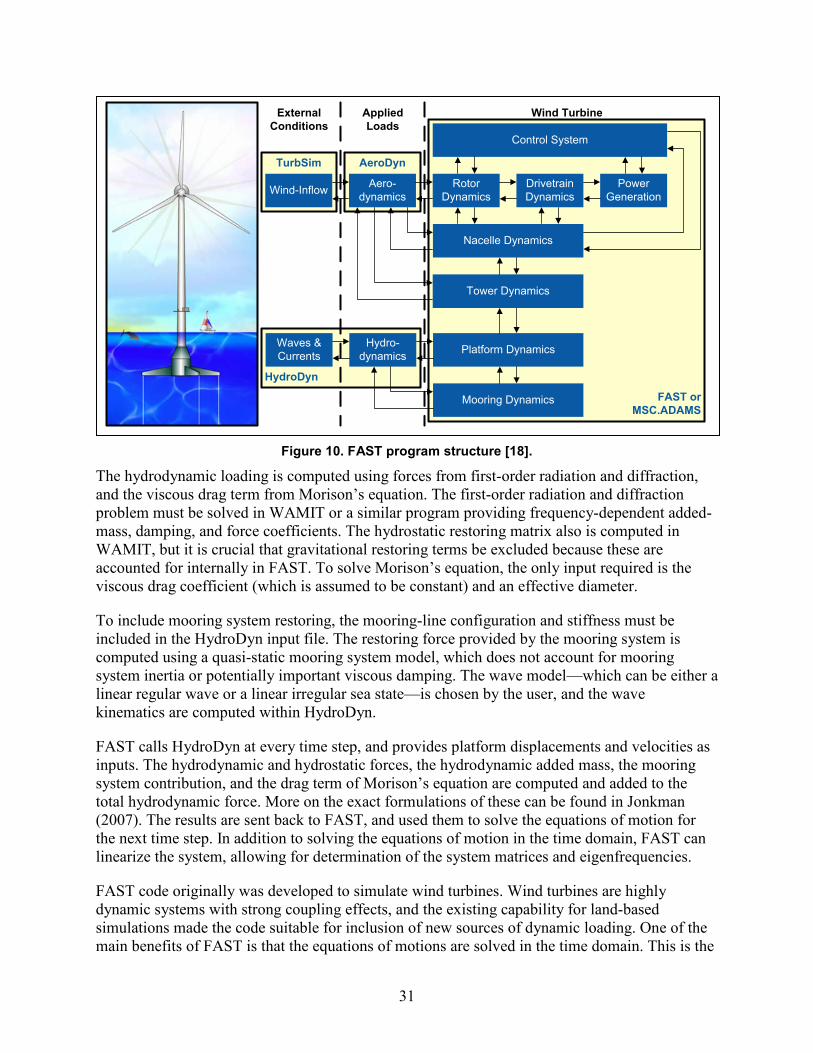
31
Figure 10. FAST program structure [18].
The hydrodynamic loading is computed using forces from first-order radiation and diffraction, and the viscous drag term from Morison’s equation. The first-order radiation and diffraction problem must be solved in WAMIT or a similar program providing frequency-dependent added-mass, damping, and force coefficients. The hydrostatic restoring matrix also is computed in WAMIT, but it is crucial that gravitational restoring terms be excluded because these are accounted for internally in FAST. To solve Morison’s equation, the only input required is the viscous drag coefficient (which is assumed to be constant) and an effective diameter.
To include mooring system restoring, the mooring-line configuration and stiffness must be included in the HydroDyn input file. The restoring force provided by the mooring system is computed using a quasi-static mooring system model, which does not account for mooring system inertia or potentially important viscous damping. The wave model—which can be either a linear regular wave or a linear irregular sea state—is chosen by the user, and the wave kinematics are computed within HydroDyn.
FAST calls HydroDyn at every time step, and provides platform displacements and velocities as inputs. The hydrodynamic and hydrostatic forces, the hydrodynamic added mass, the mooring system contribution, and the drag term of Morison’s equation are computed and added to the total hydrodynamic force. More on the exact formulations of these can be found in Jonkman (2007). The results are sent back to FAST, and used them to solve the equations of motion for the next time step. In addition to solving the equations of motion in the time domain, FAST can linearize the system, allowing for determination of the system matrices and eigenfrequencies.
FAST code originally was developed to simulate wind turbines. Wind turbines are highly dynamic systems with strong coupling effects, and the existing capability for land-based simulations made the code suitable for inclusion of new sources of dynamic loading. One of the main benefits of FAST is that the equations of motions are solved in the time domain. This is the
FAST orMSC.ADAMS
HydroDyn
AeroDyn
External Conditions
Applied Loads
Wind Turbine
TurbSim
Hydro-dynamics
Aero-dynamics
Waves & Currents
Wind-Inflow Power Generation
Rotor Dynamics
Platform Dynamics
Mooring Dynamics
Drivetrain Dynamics
Control System
Nacelle Dynamics
Tower Dynamics
32
key characteristic that allows for inclusion of transient behavior and coupled dynamics of the platform, tower, and rotor. The main limitation of FAST in this context is that it cannot include the influence of second-order hydrodynamics. For wave loading, FAST depends mainly on linear coefficients that must be generated externally. Another limitation is that it is not possible to include wave spreading in the wave model, and all sea states therefore are modeled as long-crested seas.
3.2 Wave Analysis at Massachusetts Institute of Technology (WAMIT) Wave Analysis at MIT (WAMIT) is a three-dimensional panel code designed to compute hydrodynamic loading from the radiation and diffraction problem in the frequency domain. It is a commercial code that is used widely in the offshore industry, and is capable of solving both the first-order and second-order hydrodynamic problem for a structure with arbitrary geometry.
When solving the first-order problem with WAMIT, possible outputs include added-mass, damping, and first-order wave excitation force coefficients. The hydrostatic restoring matrix is a default output, and there are several other options to select output fluid-domain properties such as fluid pressure or particle velocities. The motion RAOs (defined by Equation 2–56, also can be chosen as an output. Moreover, the second-order mean-drift force can be computed as part of the first-order problem, because it depends on quadratic contributions from the first-order potential only. Solving the second-order problem with WAMIT provides second-order force QTFs and second-order motion QTFs. It also is possible to output other properties, e.g., the second-order pressure or incident wave elevation.
The specific incident wave frequencies and wave headings for which the radiation and diffraction problem should be solved must be specified to generate any output from WAMIT. It is important to choose wave frequencies that at least cover the most important range (i.e., with the highest wave energy levels) from 0.25 to 1.25 rad/s. In many cases, a broader range of frequencies is needed, e.g., when WAMIT output is used as an input to FAST. For the frequency-to-time-domain transforms used within HydroDyn to work correctly, frequencies up to 5 rad/s typically are needed. The second-order problem must be solved for all pairs of wave frequencies, therefore the number of frequencies should be kept relatively small for a second-order simulation to keep computational efforts within bounds.
A suitable representation of the body geometry is needed to run WAMIT. Depending on the type of simulation used, the geometry can be modeled by a mesh of quadrilateral panels or by using more sophisticated methods, such as a CAD model from MultiSurf. In this report, the geometry usually is modeled with quadrilateral panels. WAMIT is indifferent to anything above the surface, therefore only the geometry of the platform below the waterline must be modeled. To prevent numerical errors at high frequencies and avoid problems with non-physical waves, the free-surface inside the body also should be meshed. For the second-order problem, the free-surface outside the body also must be meshed to allow the inhomogeneous free-surface condition to be enforced.
To ensure that the chosen discretization is sufficient for obtaining meaningful results, a convergence test should be performed. This is done by running a set of simulations in which the discretization is consistently refined. The accuracy of the first-order quantities primarily is influenced by the number of body panels. The arrangement of the panels also has a smaller
33
impact on the accuracy. Cosine spacing from the waterline to the draft is regarded as the meshing method that gives the most accurate results for a given number of panels. The second-order quantities are influenced by both body discretization and free-surface discretization, so the convergence should be tested for both.
If the first-order motion RAOs are required as an output, then WAMIT must solve for equations of motion. For this purpose, the center of mass and the system inertia, external damping, and external stiffness matrices must be specified. It is important to be aware that formulating the second-order potential requires the first-order body motions as an input, and that the system matrices always must be specified for a second-order simulation.
The damping and stiffness matrices referred to as external contain all damping and stiffness contributions that are not due to hydrodynamic effects, such as mooring system stiffness and aerodynamic damping from a wind turbine. If the body is freely floating without any external damping or stiffness, the system inertia can be specified by the radii of gyration and the vertical position of the center of gravity. The rest is calculated within WAMIT. In any other case, the full 6 x 6 matrices for mass, external damping, and external stiffness must be input. The matrices should account for the inertia and stiffness and damping effects that are induced by the turbine mounted on top of the platform, although this turbine is not modeled in WAMIT. It also should account for mooring-system stiffness. These matrices can be computed through a linearization of the wind turbine model in FAST, however, they only are approximate representations of the unsteady aerodynamic loading or the non-linear mooring-system stiffness of a real turbine.
The WAMIT code originally was created to compute hydrodynamic loading for structures where other sources of loading are negligible in comparison, and where the platform natural frequencies and first-order wave frequencies are the only frequencies important to the motion response. These assumptions might be viable for an oil platform or a ship, but are problematic for analyzing turbines.
The frequency-domain approach assumes a periodic steady-state motion that is not viable for a turbine that is subject to unsteady aerodynamic loading. This means that the motion response calculated in WAMIT only is an approximation of the true response, since the aerodynamic forces are not accounted for. For first-order simulations, this problem can be avoided by using only the frequency-domain forces (calculated at the mean position of the body) as an input to the time-domain simulations, which is t the approach taken in FAST.
For second-order simulations it is more difficult to get around the inaccuracies of the frequency-domain calculations. The formulation of the second-order problem requires knowledge about first-order motions. Because only hydrodynamic loading is included in WAMIT, the first-order motions calculated internally in WAMIT do not include motion contributions from aerodynamics. This means that the second-order hydrodynamic force is computed without accounting for any motions due to aerodynamics. For the calculation of the second-order forces, this is however acceptable if the motion amplitudes of the platform are not too great.
Another consequence of computing the motion amplitudes in WAMIT is that only the platform degrees of freedom can be included. For a large turbine with a high tower, the tower-bending frequency comes into a range where it starts interacting with platform eigenfrequencies. The
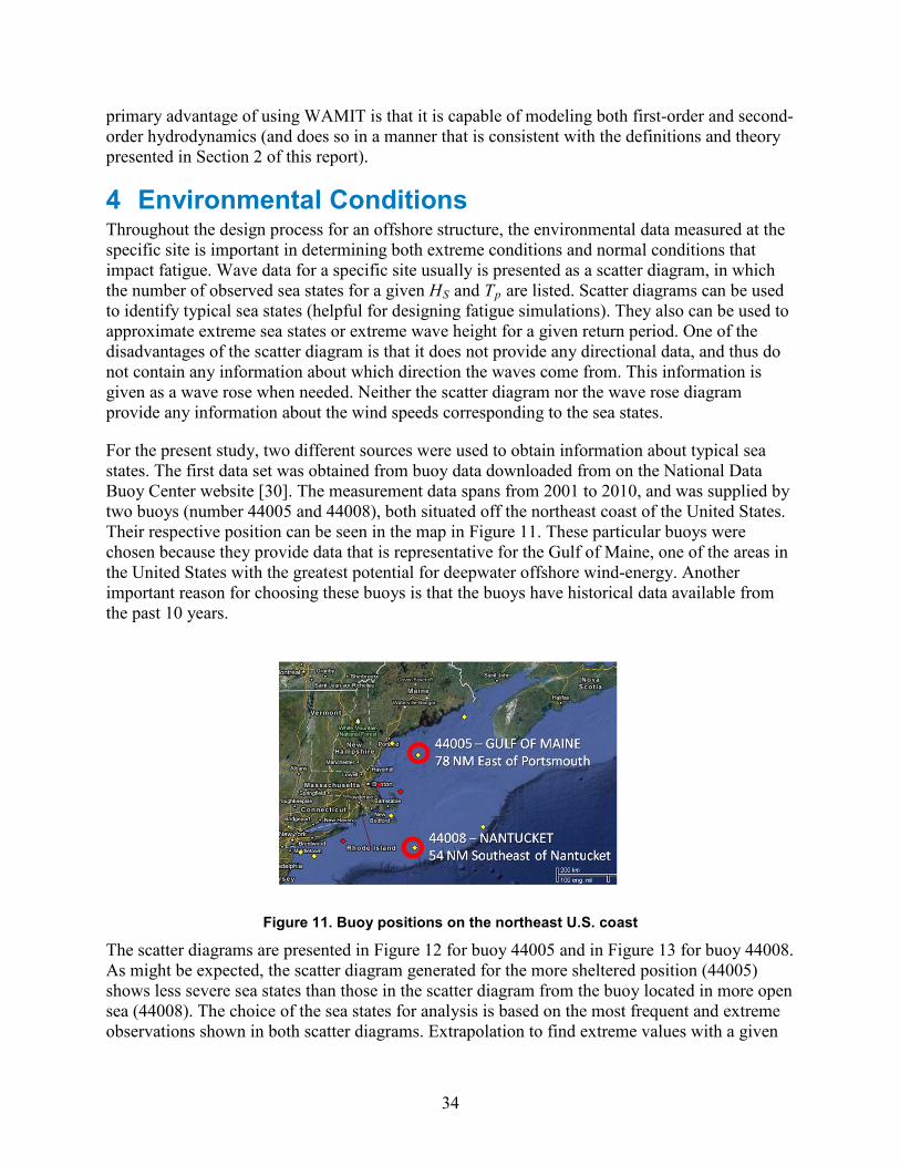
34
primary advantage of using WAMIT is that it is capable of modeling both first-order and second-order hydrodynamics (and does so in a manner that is consistent with the definitions and theory presented in Section 2 of this report).
4 Environmental Conditions Throughout the design process for an offshore structure, the environmental data measured at the specific site is important in determining both extreme conditions and normal conditions that impact fatigue. Wave data for a specific site usually is presented as a scatter diagram, in which the number of observed sea states for a given HS and Tp are listed. Scatter diagrams can be used to identify typical sea states (helpful for designing fatigue simulations). They also can be used to approximate extreme sea states or extreme wave height for a given return period. One of the disadvantages of the scatter diagram is that it does not provide any directional data, and thus do not contain any information about which direction the waves come from. This information is given as a wave rose when needed. Neither the scatter diagram nor the wave rose diagram provide any information about the wind speeds corresponding to the sea states.
For the present study, two different sources were used to obtain information about typical sea states. The first data set was obtained from buoy data downloaded from on the National Data Buoy Center website [30]. The measurement data spans from 2001 to 2010, and was supplied by two buoys (number 44005 and 44008), both situated off the northeast coast of the United States. Their respective position can be seen in the map in Figure 11. These particular buoys were chosen because they provide data that is representative for the Gulf of Maine, one of the areas in the United States with the greatest potential for deepwater offshore wind-energy. Another important reason for choosing these buoys is that the buoys have historical data available from the past 10 years.
Figure 11. Buoy positions on the northeast U.S. coast
The scatter diagrams are presented in Figure 12 for buoy 44005 and in Figure 13 for buoy 44008. As might be expected, the scatter diagram generated for the more sheltered position (44005) shows less severe sea states than those in the scatter diagram from the buoy located in more open sea (44008). The choice of the sea states for analysis is based on the most frequent and extreme observations shown in both scatter diagrams. Extrapolation to find extreme values with a given
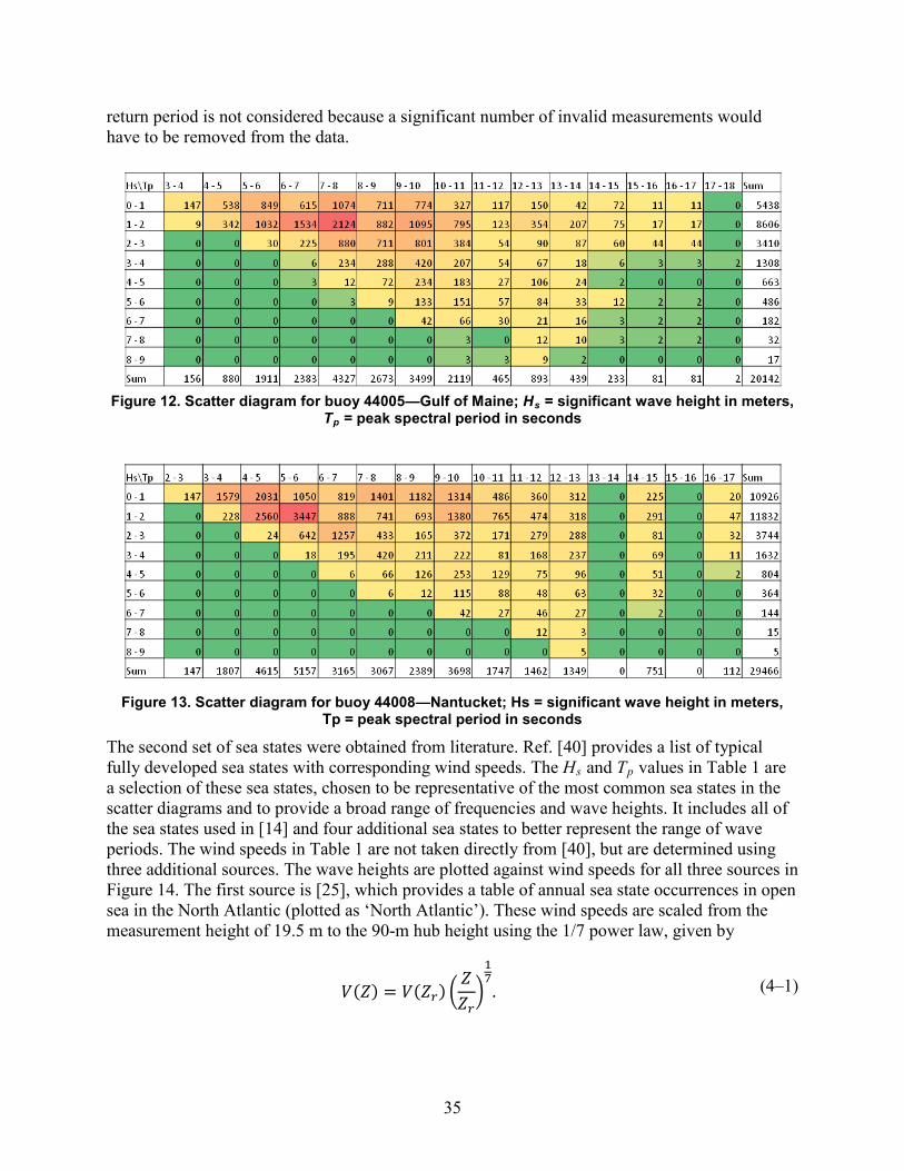
35
return period is not considered because a significant number of invalid measurements would have to be removed from the data.
Figure 12. Scatter diagram for buoy 44005—Gulf of Maine; Hs = significant wave height in meters, Tp = peak spectral period in seconds
Figure 13. Scatter diagram for buoy 44008—Nantucket; Hs = significant wave height in meters, Tp = peak spectral period in seconds
The second set of sea states were obtained from literature. Ref. [40] provides a list of typical fully developed sea states with corresponding wind speeds. The Hs and Tp values in Table 1 are a selection of these sea states, chosen to be representative of the most common sea states in the scatter diagrams and to provide a broad range of frequencies and wave heights. It includes all of the sea states used in [14] and four additional sea states to better represent the range of wave periods. The wind speeds in Table 1 are not taken directly from [40], but are determined using three additional sources. The wave heights are plotted against wind speeds for all three sources in Figure 14. The first source is [25], which provides a table of annual sea state occurrences in open sea in the North Atlantic (plotted as ‘North Atlantic’). These wind speeds are scaled from the measurement height of 19.5 m to the 90-m hub height using the 1/7 power law, given by
𝑉(𝑍) = 𝑉(𝑍𝑟) �𝑍𝑍𝑟�17
. (4–1)
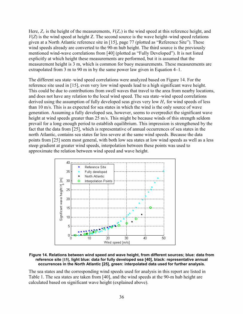
36
Here, Zr is the height of the measurements, V(Zr) is the wind speed at this reference height, and V(Z) is the wind speed at height Z. The second source is the wave height–wind speed relations given at a North Atlantic reference site in [15], page 77 (plotted as “Reference Site”). These wind speeds already are converted to the 90-m hub height. The third source is the previously mentioned wind-wave correlations from [40] (plotted as “Fully Developed”). It is not listed explicitly at which height these measurements are performed, but it is assumed that the measurement height is 3 m, which is common for buoy measurements. These measurements are extrapolated from 3 m to 90 m in by the same power law given in Equation 4–1.
The different sea state–wind speed correlations were analyzed based on Figure 14. For the reference site used in [15], even very low wind speeds lead to a high significant wave height. This could be due to contributions from swell waves that travel to the area from nearby locations, and does not have any relation to the local wind speed. The sea state–wind speed correlations derived using the assumption of fully developed seas gives very low Hs for wind speeds of less than 10 m/s. This is as expected for sea states in which the wind is the only source of wave generation. Assuming a fully developed sea, however, seems to overpredict the significant wave height at wind speeds greater than 25 m/s. This might be because winds of this strength seldom prevail for a long enough period to establish equilibrium. This impression is strengthened by the fact that the data from [25], which is representative of annual occurrences of sea states in the north Atlantic, contains sea states far less severe at the same wind speeds. Because the data points from [25] seem most general, with both low sea states at low wind speeds as well as a less steep gradient at greater wind speeds, interpolation between these points was used to approximate the relation between wind speed and wave height.
Figure 14. Relations between wind speed and wave height, from different sources; blue: data from
reference site [15], light blue: data for fully developed sea [40], black: representative annual occurrences in the North Atlantic [25], green: interpolated data used for further analysis.
The sea states and the corresponding wind speeds used for analysis in this report are listed in Table 1. The sea states are taken from [40], and the wind speeds at the 90-m hub height are calculated based on significant wave height (explained above).
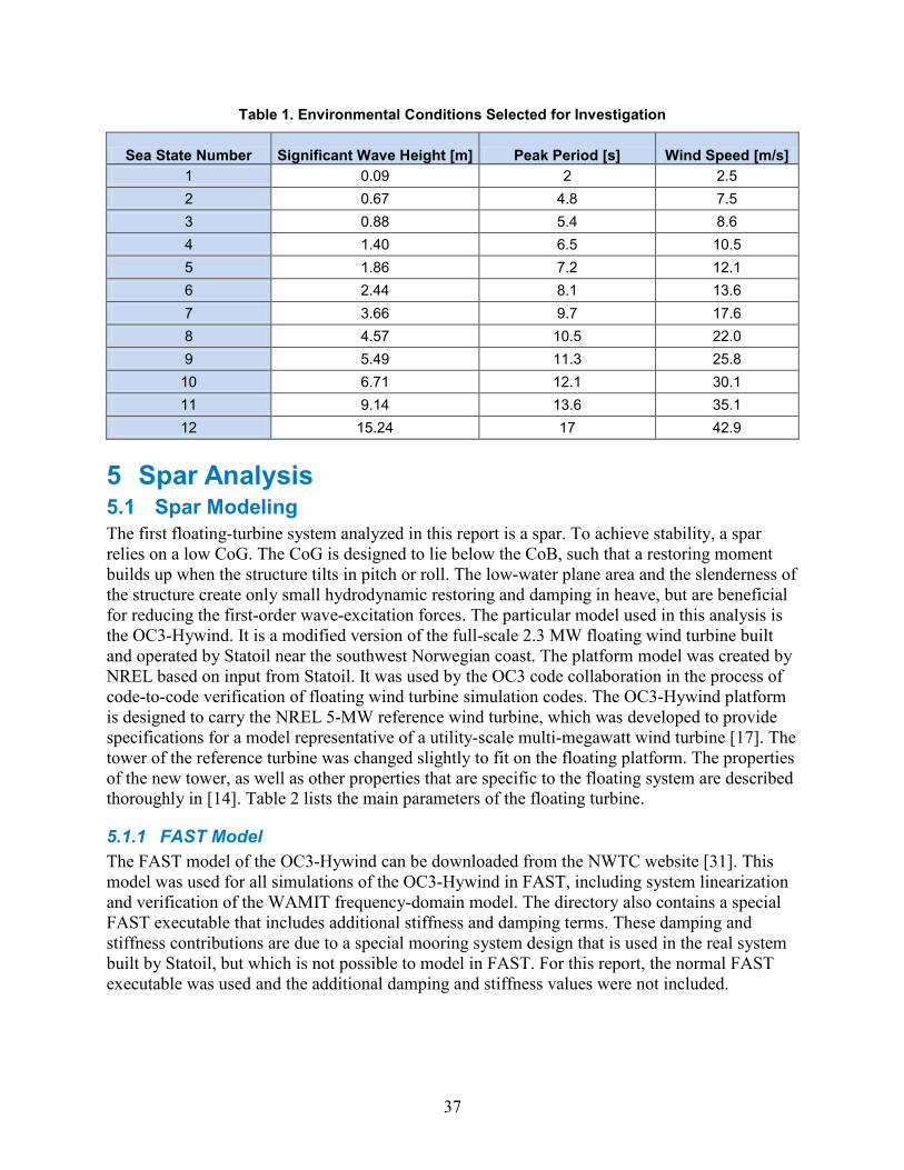
37
Table 1. Environmental Conditions Selected for Investigation
Sea State Number Significant Wave Height [m] Peak Period [s] Wind Speed [m/s] 1 0.09 2 2.5 2 0.67 4.8 7.5 3 0.88 5.4 8.6 4 1.40 6.5 10.5 5 1.86 7.2 12.1 6 2.44 8.1 13.6 7 3.66 9.7 17.6 8 4.57 10.5 22.0 9 5.49 11.3 25.8
10 6.71 12.1 30.1 11 9.14 13.6 35.1 12 15.24 17 42.9
5 Spar Analysis 5.1 Spar Modeling The first floating-turbine system analyzed in this report is a spar. To achieve stability, a spar relies on a low CoG. The CoG is designed to lie below the CoB, such that a restoring moment builds up when the structure tilts in pitch or roll. The low-water plane area and the slenderness of the structure create only small hydrodynamic restoring and damping in heave, but are beneficial for reducing the first-order wave-excitation forces. The particular model used in this analysis is the OC3-Hywind. It is a modified version of the full-scale 2.3 MW floating wind turbine built and operated by Statoil near the southwest Norwegian coast. The platform model was created by NREL based on input from Statoil. It was used by the OC3 code collaboration in the process of code-to-code verification of floating wind turbine simulation codes. The OC3-Hywind platform is designed to carry the NREL 5-MW reference wind turbine, which was developed to provide specifications for a model representative of a utility-scale multi-megawatt wind turbine [17]. The tower of the reference turbine was changed slightly to fit on the floating platform. The properties of the new tower, as well as other properties that are specific to the floating system are described thoroughly in [14]. Table 2 lists the main parameters of the floating turbine.
5.1.1 FAST Model The FAST model of the OC3-Hywind can be downloaded from the NWTC website [31]. This model was used for all simulations of the OC3-Hywind in FAST, including system linearization and verification of the WAMIT frequency-domain model. The directory also contains a special FAST executable that includes additional stiffness and damping terms. These damping and stiffness contributions are due to a special mooring system design that is used in the real system built by Statoil, but which is not possible to model in FAST. For this report, the normal FAST executable was used and the additional damping and stiffness values were not included.
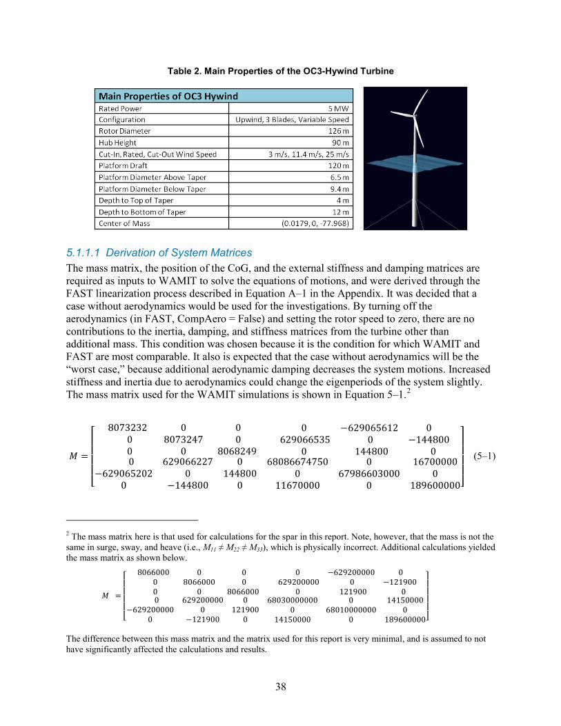
38
Table 2. Main Properties of the OC3-Hywind Turbine
5.1.1.1 Derivation of System Matrices The mass matrix, the position of the CoG, and the external stiffness and damping matrices are required as inputs to WAMIT to solve the equations of motions, and were derived through the FAST linearization process described in Equation A–1 in the Appendix. It was decided that a case without aerodynamics would be used for the investigations. By turning off the aerodynamics (in FAST, CompAero = False) and setting the rotor speed to zero, there are no contributions to the inertia, damping, and stiffness matrices from the turbine other than additional mass. This condition was chosen because it is the condition for which WAMIT and FAST are most comparable. It also is expected that the case without aerodynamics will be the “worst case,” because additional aerodynamic damping decreases the system motions. Increased stiffness and inertia due to aerodynamics could change the eigenperiods of the system slightly. The mass matrix used for the WAMIT simulations is shown in Equation 5–1.2
𝑀 =
⎣⎢⎢⎢⎢⎡ 8073232 0 0
0 8073247 0 0 0 8068249
0 −629065612 0 629066535 0 −144800
0 144800 0 0 629066227 0
−629065202 0 1448000 −144800 0
68086674750 0 167000000 67986603000 0
11670000 0 189600000⎦⎥⎥⎥⎥⎤
(5–1)
2 The mass matrix here is that used for calculations for the spar in this report. Note, however, that the mass is not the same in surge, sway, and heave (i.e., M11 ≠ M22 ≠ M33), which is physically incorrect. Additional calculations yielded the mass matrix as shown below.
𝑀 =
⎣⎢⎢⎢⎢⎡ 8066000 0 0
0 8066000 0 0 0 8066000
0 −629200000 0 629200000 0 −121900
0 121900 0 0 629200000 0
−629200000 0 1219000 −121900 0
68030000000 0 141500000 68010000000 0
14150000 0 189600000⎦⎥⎥⎥⎥⎤
The difference between this mass matrix and the matrix used for this report is very minimal, and is assumed to not have significantly affected the calculations and results.
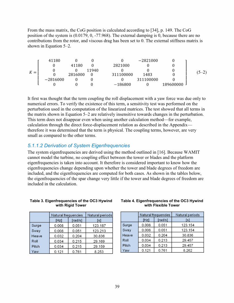
39
From the mass matrix, the CoG position is calculated according to [34], p. 149. The CoG position of the system is (0.0179, 0, -77.968). The external damping is 0, because there are no contributions from the rotor, and viscous drag has been set to 0. The external stiffness matrix is shown in Equation 5–2.
𝐾 =
⎣⎢⎢⎢⎢⎡ 41180 0 0
0 41180 0 0 0 11940
0 −2821000 0 2821000 0 0
0 0 00 2816000 0
−2816000 0 00 0 0
311100000 1483 0
0 311100000 0−186800 0 189600000 ⎦
⎥⎥⎥⎥⎤
(5–2)
It first was thought that the term coupling the roll displacement with a yaw force was due only to numerical errors. To verify the existence of this term, a sensitivity test was performed on the perturbation used in the computation of the linearized matrices. The test showed that all terms in the matrix shown in Equation 5–2 are relatively insensitive towards changes in the perturbation. This term does not disappear even when using another calculation method—for example, calculation through the direct force-displacement relation as described in the Appendix—therefore it was determined that the term is physical. The coupling terms, however, are very small as compared to the other terms.
5.1.1.2 Derivation of System Eigenfrequencies The system eigenfrequencies are derived using the method outlined in [16]. Because WAMIT cannot model the turbine, no coupling effect between the tower or blades and the platform eigenfrequencies is taken into account. It therefore is considered important to know how the eigenfrequencies change depending upon whether the tower and blade degrees of freedom are included, and the eigenfrequencies are computed for both cases. As shown in the tables below, the eigenfrequencies of the spar change very little if the tower and blade degrees of freedom are included in the calculation.
Table 3. Eigenfrequencies of the OC3 Hywind
with Rigid Tower
Table 4. Eigenfrequencies of the OC3 Hywind with Flexible Tower
40
5.1.2 WAMIT Model The geometry of the Hywind is modeled with quadrilateral panels. The spar has two planes of symmetry, therefore only one quarter of the structure must be modeled, leading to shorter simulation time within WAMIT. To achieve more accurate results from the simulations, use cosine spacing for the panels that are close to sharp edges or close to the free surface (this is especially important for second-order hydrodynamic loads). The geometric data file which contains the coordinates of the four vertices of each panel is generated using a MatLab script. This script is based on an existing script developed by Jonkman, but required modification to create a cosine-spaced mesh.
5.1.2.1 First-Order Convergence Tests To determine how many panels are needed to model the structure and to get an overall impression of the accuracy of the results, a common procedure is to perform a convergence test in WAMIT. This test helps to assess the convergence of the results with finer discretizations. The accuracy of the first-order quantities (added mass, hydrodynamic damping, and first-order excitation force coefficients) is influenced almost only by the number of body panels. The arrangement of the panels also has a lesser impact on the accuracy, with cosine spacing from the waterline to the draft regarded as the meshing method and producing the most accurate results for a given number of panels.
The first-order convergence tests are performed with regard to the number of body panels and always with cosine spacing. As suggested in literature, four different meshes where the panel size is reduced consistently from one mesh to another were used. The length of the panel sides was halved in both directions from a coarser to a finer discretization. The four meshes had respectively 195; 931; 4,035; and 9,315 body panels to represent a quarter of the spar. The mesh for the 931 panels is shown in Figure 15.
Convergence tests are performed for added-mass and hydrodynamic-damping coefficients, as well as for wave-excitation force coefficients. These coefficients are frequency dependent, therefore the test must be performed for a range of frequencies. Wave periods from 5 s to 25 s are chosen, because these are the periods at which ocean waves contain significant energy. Also, the zero-frequency and infinite-frequency limits are compared (although these are non-zero only for the added mass). Due to the symmetry of the spar, only head-on waves are considered. To illustrate the results from the tests, values for the damping coefficient B33 is shown in Figure 16.
In the case using 4,035 panels, the simulation results have converged to within 1% for all values (with the solution for 9,315 panels used as a reference value). The situation is the same for 931 panels except for damping in heave, for which the difference is less than 2%. These results only are valid if yaw added mass and damping are not taken into account. The value of yaw added mass and damping are in the order of 10-19, such that even though the results do not converge consistently, the effect of the differences is insignificant. The differences are assumed to be due to the inaccuracies that arise from representing a curved surface with flat panels.
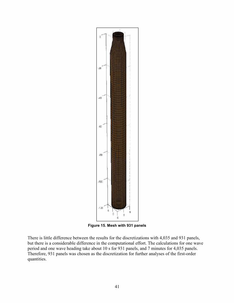
41
Figure 15. Mesh with 931 panels
There is little difference between the results for the discretizations with 4,035 and 931 panels, but there is a considerable difference in the computational effort. The calculations for one wave period and one wave heading take about 10 s for 931 panels, and 7 minutes for 4,035 panels. Therefore, 931 panels was chosen as the discretization for further analyses of the first-order quantities.
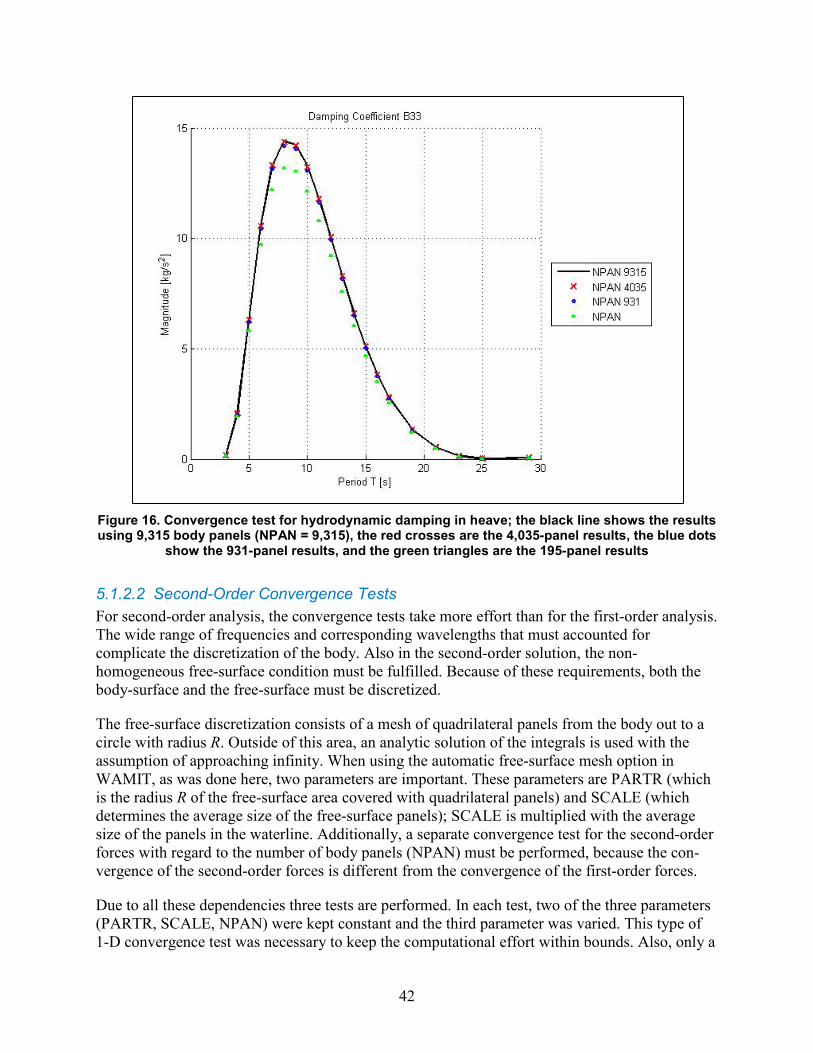
42
Figure 16. Convergence test for hydrodynamic damping in heave; the black line shows the results using 9,315 body panels (NPAN = 9,315), the red crosses are the 4,035-panel results, the blue dots
show the 931-panel results, and the green triangles are the 195-panel results
5.1.2.2 Second-Order Convergence Tests For second-order analysis, the convergence tests take more effort than for the first-order analysis. The wide range of frequencies and corresponding wavelengths that must accounted for complicate the discretization of the body. Also in the second-order solution, the non-homogeneous free-surface condition must be fulfilled. Because of these requirements, both the body-surface and the free-surface must be discretized.
The free-surface discretization consists of a mesh of quadrilateral panels from the body out to a circle with radius R. Outside of this area, an analytic solution of the integrals is used with the assumption of approaching infinity. When using the automatic free-surface mesh option in WAMIT, as was done here, two parameters are important. These parameters are PARTR (which is the radius R of the free-surface area covered with quadrilateral panels) and SCALE (which determines the average size of the free-surface panels); SCALE is multiplied with the average size of the panels in the waterline. Additionally, a separate convergence test for the second-order forces with regard to the number of body panels (NPAN) must be performed, because the con-vergence of the second-order forces is different from the convergence of the first-order forces.
Due to all these dependencies three tests are performed. In each test, two of the three parameters (PARTR, SCALE, NPAN) were kept constant and the third parameter was varied. This type of 1-D convergence test was necessary to keep the computational effort within bounds. Also, only a
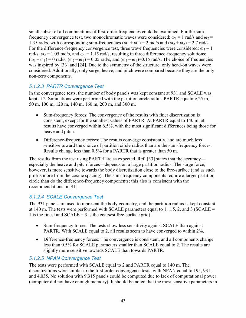
43
small subset of all combinations of first-order frequencies could be examined. For the sum-frequency convergence test, two monochromatic waves were considered: ω1 = 1 rad/s and ω2 = 1.35 rad/s, with corresponding sum-frequencies (ω1 + ω1) = 2 rad/s and (ω2 + ω2) = 2.7 rad/s. For the difference-frequency convergence test, three wave frequencies were considered: ω1 = 1 rad/s, ω2 = 1.05 rad/s, and ω3 = 1.15 rad/s, resulting in three difference-frequency solutions: (ω1 – ω1) = 0 rad/s, (ω2 – ω1) = 0.05 rad/s, and (ω3 – ω1)=0.15 rad/s. The choice of frequencies was inspired by [33] and [24]. Due to the symmetry of the structure, only head-on waves were considered. Additionally, only surge, heave, and pitch were compared because they are the only non-zero components.
5.1.2.3 PARTR Convergence Test In the convergence tests, the number of body panels was kept constant at 931 and SCALE was kept at 2. Simulations were performed with the partition circle radius PARTR equaling 25 m, 50 m, 100 m, 120 m, 140 m, 160 m, 200 m, and 300 m.
• Sum-frequency forces: The convergence of the results with finer discretization is consistent, except for the smallest values of PARTR. At PARTR equal to 140 m, all results have converged within 6.5%, with the most significant differences being those for heave and pitch.
• Difference-frequency forces: The results converge consistently, and are much less sensitive toward the choice of partition circle radius than are the sum-frequency forces. Results change less than 0.5% for a PARTR that is greater than 50 m.
The results from the test using PARTR are as expected. Ref. [33] states that the accuracy—especially the heave and pitch forces—depends on a large partition radius. The surge force, however, is more sensitive towards the body discretization close to the free-surface (and as such profits more from the cosine spacing). The sum-frequency components require a larger partition circle than do the difference-frequency components; this also is consistent with the recommendations in [41].
5.1.2.4 SCALE Convergence Test The 931 panels are used to represent the body geometry, and the partition radius is kept constant at 140 m. The tests were performed with SCALE parameters equal to 1, 1.5, 2, and 3 (SCALE = 1 is the finest and SCALE = 3 is the coarsest free-surface grid).
• Sum-frequency forces: The tests show less sensitivity against SCALE than against PARTR. With SCALE equal to 2, all results seem to have converged to within 2%.
• Difference-frequency forces: The convergence is consistent, and all components change less than 0.5% for SCALE parameters smaller than SCALE equal to 2. The results are slightly more sensitive towards SCALE than towards PARTR.
5.1.2.5 NPAN Convergence Test The tests were performed with SCALE equal to 2 and PARTR equal to 140 m. The discretizations were similar to the first-order convergence tests, with NPAN equal to 195, 931, and 4,035. No solution with 9,315 panels could be computed due to lack of computational power (computer did not have enough memory). It should be noted that the most sensitive parameters in
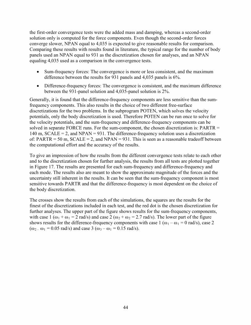
44
the first-order convergence tests were the added mass and damping, whereas a second-order solution only is computed for the force components. Even though the second-order forces converge slower, NPAN equal to 4,035 is expected to give reasonable results for comparison. Comparing these results with results found in literature, the typical range for the number of body panels used an NPAN equal to 931 as the discretization chosen for analyses, and an NPAN equaling 4,035 used as a comparison in the convergence tests.
• Sum-frequency forces: The convergence is more or less consistent, and the maximum difference between the results for 931 panels and 4,035 panels is 6%.
• Difference-frequency forces: The convergence is consistent, and the maximum difference between the 931-panel solution and 4,035-panel solution is 2%.
Generally, it is found that the difference-frequency components are less sensitive than the sum-frequency components. This also results in the choice of two different free-surface discretizations for the two problems. In the subprogram POTEN, which solves the velocity potentials, only the body discretization is used. Therefore POTEN can be run once to solve for the velocity potentials, and the sum-frequency and difference-frequency components can be solved in separate FORCE runs. For the sum-component, the chosen discretization is: PARTR = 140 m, SCALE = 2, and NPAN = 931. The difference-frequency solution uses a discretization of: PARTR = 50 m, SCALE = 2, and NPAN = 931. This is seen as a reasonable tradeoff between the computational effort and the accuracy of the results.
To give an impression of how the results from the different convergence tests relate to each other and to the discretization chosen for further analysis, the results from all tests are plotted together in Figure 17. The results are presented for each sum-frequency and difference-frequency and each mode. The results also are meant to show the approximate magnitude of the forces and the uncertainty still inherent in the results. It can be seen that the sum-frequency component is most sensitive towards PARTR and that the difference-frequency is most dependent on the choice of the body discretization.
The crosses show the results from each of the simulations, the squares are the results for the finest of the discretizations included in each test, and the red dot is the chosen discretization for further analyses. The upper part of the figure shows results for the sum-frequency components, with case 1 (ω1 + ω1 = 2 rad/s) and case 2 (ω2 + ω2 = 2.7 rad/s). The lower part of the figure shows results for the difference-frequency components with case 1 (ω1 – ω1 = 0 rad/s), case 2 (ω2 – ω1 = 0.05 rad/s) and case 3 (ω3 – ω1 = 0.15 rad/s).
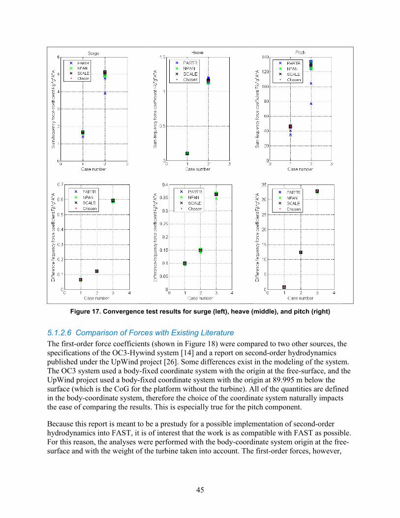
45
Figure 17. Convergence test results for surge (left), heave (middle), and pitch (right)
5.1.2.6 Comparison of Forces with Existing Literature The first-order force coefficients (shown in Figure 18) were compared to two other sources, the specifications of the OC3-Hywind system [14] and a report on second-order hydrodynamics published under the UpWind project [26]. Some differences exist in the modeling of the system. The OC3 system used a body-fixed coordinate system with the origin at the free-surface, and the UpWind project used a body-fixed coordinate system with the origin at 89.995 m below the surface (which is the CoG for the platform without the turbine). All of the quantities are defined in the body-coordinate system, therefore the choice of the coordinate system naturally impacts the ease of comparing the results. This is especially true for the pitch component.
Because this report is meant to be a prestudy for a possible implementation of second-order hydrodynamics into FAST, it is of interest that the work is as compatible with FAST as possible. For this reason, the analyses were performed with the body-coordinate system origin at the free-surface and with the weight of the turbine taken into account. The first-order forces, however,
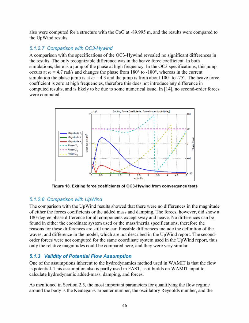
46
also were computed for a structure with the CoG at -89.995 m, and the results were compared to the UpWind results.
5.1.2.7 Comparison with OC3-Hywind A comparison with the specifications of the OC3-Hywind revealed no significant differences in the results. The only recognizable difference was in the heave force coefficient. In both simulations, there is a jump of the phase at high frequency. In the OC3 specifications, this jump occurs at ω = 4.7 rad/s and changes the phase from 180° to -180°, whereas in the current simulation the phase jump is at ω = 4.3 and the jump is from about 100° to -75°. The heave force coefficient is zero at high frequencies, therefore this does not introduce any difference in computed results, and is likely to be due to some numerical issue. In [14], no second-order forces were computed.
Figure 18. Exiting force coefficients of OC3-Hywind from convergence tests
5.1.2.8 Comparison with UpWind The comparison with the UpWind results showed that there were no differences in the magnitude of either the forces coefficients or the added mass and damping. The forces, however, did show a 180-degree phase difference for all components except sway and heave. No differences can be found in either the coordinate system used or the mass/inertia specifications, therefore the reasons for these differences are still unclear. Possible differences include the definition of the waves, and difference in the model, which are not described in the UpWind report. The second-order forces were not computed for the same coordinate system used in the UpWind report, thus only the relative magnitudes could be compared here, and they were very similar.
5.1.3 Validity of Potential Flow Assumption One of the assumptions inherent to the hydrodynamics method used in WAMIT is that the flow is potential. This assumption also is partly used in FAST, as it builds on WAMIT input to calculate hydrodynamic added-mass, damping, and forces.
As mentioned in Section 2.5, the most important parameters for quantifying the flow regime around the body is the Keulegan-Carpenter number, the oscillatory Reynolds number, and the
47
diameter to wavelength ratio. These parameters were evaluated for the OC3-Hywind in different sea states in [14]. The analysis shows that flow separation occurs on the top of the spar in severe sea states (i.e., for wave heights on the order of 5.5 m), and that the potential flow assumption is valid throughout a wide range of conditions. The intention of this report, however, is not to specifically investigate extreme design sea states, but rather to assess the second-order effects as compared to the first-order effects and the influence of the wind, therefore the potential flow assumption is found to be viable. For an assessment of extreme loads, an analysis built on potential flow assumption would yield inaccurate results.
5.2 Comparison of First-Order Time-Domain and Frequency-Domain Solution
WAMIT provides frequency-dependent coefficients that describe the hydrodynamic behavior of a structure. There are two different possibilities for transforming the WAMIT results from the frequency domain into times series, as presented in Section 2.3.4. The coefficients for hydrodynamic excitation forces, added mass, damping, and hydrostatic restoring can be used to solve the equations of motion directly in time domain. Alternatively, the equations of motion can be solved in frequency domain within WAMIT and output in the form of response amplitude operators (RAOs), from which a time series can be derived through a summation.
The two different methods are based on different assumptions and have different limitations. The direct solution by WAMIT in the frequency domain is not able to account for transients or for forces other than the pure hydrodynamic. Although it might be possible to take other forces into account in other programs, all loads would have to be linear. Essentially, this means that the solution is not suitable for direct application to wind turbines, because the non-hydrodynamic forces (which often are highly non-linear) and transient events are important to wind turbine design. The direct solution in WAMIT, however, can be a useful means to perform a first assessment of the second-order hydrodynamic effects on the wind turbine, as there currently are no coupled tools that can take these into account.
Solving the time-domain equations of motion in FAST allows non-linear loading, transients, and the memory effect to be taken into account properly. The structural properties also are linearized before the equations of motion are solved in WAMIT, whereas more of the nonlinearities are directly accounted for in FAST.
A comparison between WAMIT and FAST including only first-order hydrodynamic loading (no aerodynamics or control system) has two purposes. First, it serves as a rough check that purpose-built MatLab code used to generate time series from wave spectrum input and RAOs functions correctly. The main purpose, however, is to gain a better overview of how the two solutions relate to each other. Specifically, it can help determine how well the frequency-domain and time-domain solutions fit after transients have died out, such that it can be concluded whether the memory effects and structural properties are represented well enough by the frequency-domain solution.
The OC3-Hywind was chosen for comparison. To make the two turbine models in FAST and WAMIT as similar as possible, all aerodynamics were turned off and only the platform DOFs were included in the calculation in FAST. Because WAMIT and FAST have very different ways of accounting for mooring system stiffness, the mooring system was completely removed,
48
leaving the turbine freely floating. In WAMIT, this change creates no problems, as the equations of motion are solved around a mean position. For FAST, however, omitting the mooring system created a system which is much more sensitive towards an initial in-equilibrium position. The model required two steps of tuning to avoid unnecessary transients. These tuning steps included the following:
1. Perform Still-Water Simulations. This step involves simulating the turbine in still water to tune the system mass such that the initial position can be set as close as possible to the vertical equilibrium position. If the initial vertical position is not near equilibrium, it leads to large oscillations in heave. Heave is a mode with very little damping, therefore the initial oscillations persist for a significant period of time.
2. Eliminate Oscillations In Pitch. The center of mass of the nacelle-rotor assembly is not at the center of the tower, which causes the center of mass of the entire system to be slightly offset from the centerline of the tower. This offset adds some coupling terms to the inertia matrix, such as coupling between roll and yaw, between sway and yaw, and between heave and pitch. Of these coupling terms, the coupling between heave and pitch is term with the greatest influence on the simulation. The heave oscillations that induced by the unbalanced initial condition—which appear to some extent even after the tuning in Step 1—lead to long-persisting transient motions in pitch as well. To eliminate these oscillations in pitch, the system is changed such that the turbine’s center of mass lies on the centerline of the tower. This change also was applied to the WAMIT model by linearizing the updated FAST model and running WAMIT with the new, uncoupled inertia matrix as input. Note that, even though the coupling terms mentioned above disappear, some coupling terms remain in the inertia matrix (such as the coupling between surge and pitch). What’s important is that are no modes are coupled with heave.
To create time series from WAMIT RAOs, the frequency-domain coefficients must be transformed into a time series. This is performed using MATLAB. The phrase “WAMIT time series” hereinafter is used to identify “time series created by MATLAB using WAMIT input.” To make the WAMIT time series comparable to the FAST time series, the incident waves have to be the same. The two programs, however, use different representations for the wave elevation. A relation between the formulation used in FAST and the formulation that WAMIT is based on (which also commonly is used in ocean engineering) had to be derived to determine how the complex wave amplitudes in the two programs relate. The wave elevation in FAST is calculated by
𝜁(𝑡𝑛) = 1𝑁′∑ 𝑍[𝑘]𝑒𝑗𝜔𝑘𝑡𝑛𝑁′
2
𝑘=−𝑁′2 +1
(but 𝑍 �𝑁′
2� = 0 ) , (5-3)
where ζ(tn) is the wave elevation at time step tn, N' is the number of wave frequencies used in FAST, and Z[k] is the complex wave amplitude in FAST. The theory used in WAMIT defines the wave elevation as
𝜁(𝑡𝑛) = 𝑅𝑒 ��𝑎𝑘𝑒𝑗𝜔𝑘𝑡𝑛
𝑁
𝑘=1
�, (5–4)
49
where ζ(tn) is the wave elevation at time step tn, N' is the number of wave frequencies for which a solution is computed within WAMIT, and ak is the complex wave amplitude corresponding to wave frequency k. The two formulations must be physically the same, i.e., the wave elevation at a given time must be the same regardless of whether the WAMIT or the FAST formulation is used. The relation between the complex wave amplitudes in FAST Z[k] and WAMIT ak er given as
𝜁(𝑡𝑛) = 1𝑁′ � 𝑍[𝑘]𝑒𝑗𝜔𝑘𝑡𝑛
𝑁′2 −1
𝑘=−𝑁′
2 +1
≡ 𝑅𝑒 ��𝑎𝑘𝑒𝑗𝜔𝑘𝑡𝑛
𝑁
𝑘=1
�.
(5–5)
Because Re{c} = c+c∗
2 , the left-hand side of Equation 5-5 can be expressed as
𝜁(𝑡𝑛) = 12��𝑎𝑘𝑒𝑗𝜔𝑘𝑡𝑛
𝑁
𝑘=1
+ ��𝑎𝑘𝑒𝑗𝜔𝑘𝑡𝑛
𝑁
𝑘=1
�
∗
� = 12��𝑎𝑘𝑒𝑗𝜔𝑘𝑡𝑛
𝑁
𝑘=1
+ �𝑎𝑘∗𝑒−𝑗𝜔𝑘𝑡𝑛
𝑁
𝑘=1
�
= 12��𝑎𝑘𝑒𝑗𝜔𝑘𝑡𝑛
𝑁
𝑘=1
+ � 𝑎|𝑘|∗𝑒𝑗𝜔𝑘𝑡𝑛
−1
𝑘=−𝑁
� .
(5–6)
Using ak = a|k|∗ for k < 0 and ωk = ωk , and a0 = 0 results in Equation 5–7.
𝜁(𝑡𝑛) = 12� 𝑎𝑘𝑒𝑗𝜔𝑘𝑡𝑛
𝑁
𝑘=−𝑁
(5–7)
Comparing Equation 5-7 to Equation 5-5, we get the following relations for 𝑎𝑘, 𝑍[𝑘], 𝑁 and 𝑁𝑘:
𝑎𝑘2
= 𝑍[𝑘]𝑁′
and 𝑎𝑘 = 2𝑁′𝑍[𝑘] and 𝑁 = 𝑁′
2− 1 (5–8)
With these relations, both the number of wave components and the complex wave amplitudes that are to be used in MatLab to derive time series from the WAMIT output can be derived from the FAST amplitudes. To get the amplitudes output from FAST, however, the source code must be modified. The necessary changes were provided by Bonnie Jonkman. The amplitudes probably will become a standard output option in a subsequent version of FAST/HydroDyn.
With the wave amplitudes input from FAST, a MatLab script was created to do the summation required to get time series from the RAOs, i.e, to solve Equation 2–57. In the first cases used for the comparison it was seen that due to the low damping in the system, the transients are dominant even after 10 000 s. The longest possible simulation time in FAST normally is 9 999 s, due to overflow in the output. To obtain comparable results, this had to be changed to 99 999 s. A simulation of 20 000 s was run and it is the results from the last 150 s of that simulation that are presented in Figure 19, Figure 20, and Figure 21. As can be seen from the surge and pitch time series in Figure 19 and Figure 20, there are no significant differences between the
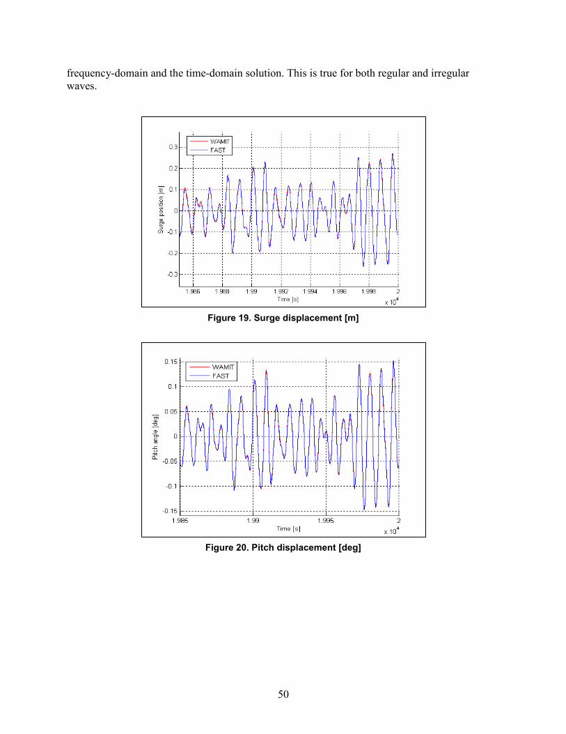
50
frequency-domain and the time-domain solution. This is true for both regular and irregular waves.
Figure 19. Surge displacement [m]
Figure 20. Pitch displacement [deg]
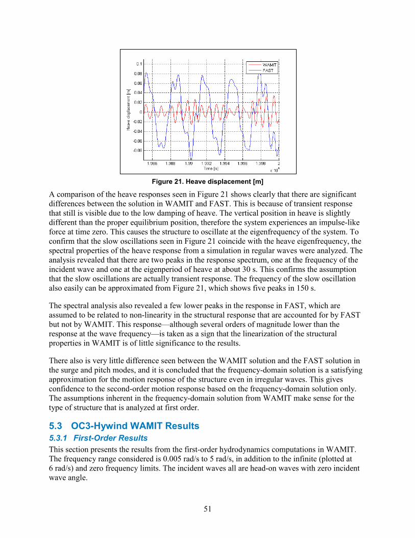
51
Figure 21. Heave displacement [m]
A comparison of the heave responses seen in Figure 21 shows clearly that there are significant differences between the solution in WAMIT and FAST. This is because of transient response that still is visible due to the low damping of heave. The vertical position in heave is slightly different than the proper equilibrium position, therefore the system experiences an impulse-like force at time zero. This causes the structure to oscillate at the eigenfrequency of the system. To confirm that the slow oscillations seen in Figure 21 coincide with the heave eigenfrequency, the spectral properties of the heave response from a simulation in regular waves were analyzed. The analysis revealed that there are two peaks in the response spectrum, one at the frequency of the incident wave and one at the eigenperiod of heave at about 30 s. This confirms the assumption that the slow oscillations are actually transient response. The frequency of the slow oscillation also easily can be approximated from Figure 21, which shows five peaks in 150 s.
The spectral analysis also revealed a few lower peaks in the response in FAST, which are assumed to be related to non-linearity in the structural response that are accounted for by FAST but not by WAMIT. This response—although several orders of magnitude lower than the response at the wave frequency—is taken as a sign that the linearization of the structural properties in WAMIT is of little significance to the results.
There also is very little difference seen between the WAMIT solution and the FAST solution in the surge and pitch modes, and it is concluded that the frequency-domain solution is a satisfying approximation for the motion response of the structure even in irregular waves. This gives confidence to the second-order motion response based on the frequency-domain solution only. The assumptions inherent in the frequency-domain solution from WAMIT make sense for the type of structure that is analyzed at first order.
5.3 OC3-Hywind WAMIT Results 5.3.1 First-Order Results This section presents the results from the first-order hydrodynamics computations in WAMIT. The frequency range considered is 0.005 rad/s to 5 rad/s, in addition to the infinite (plotted at 6 rad/s) and zero frequency limits. The incident waves all are head-on waves with zero incident wave angle.
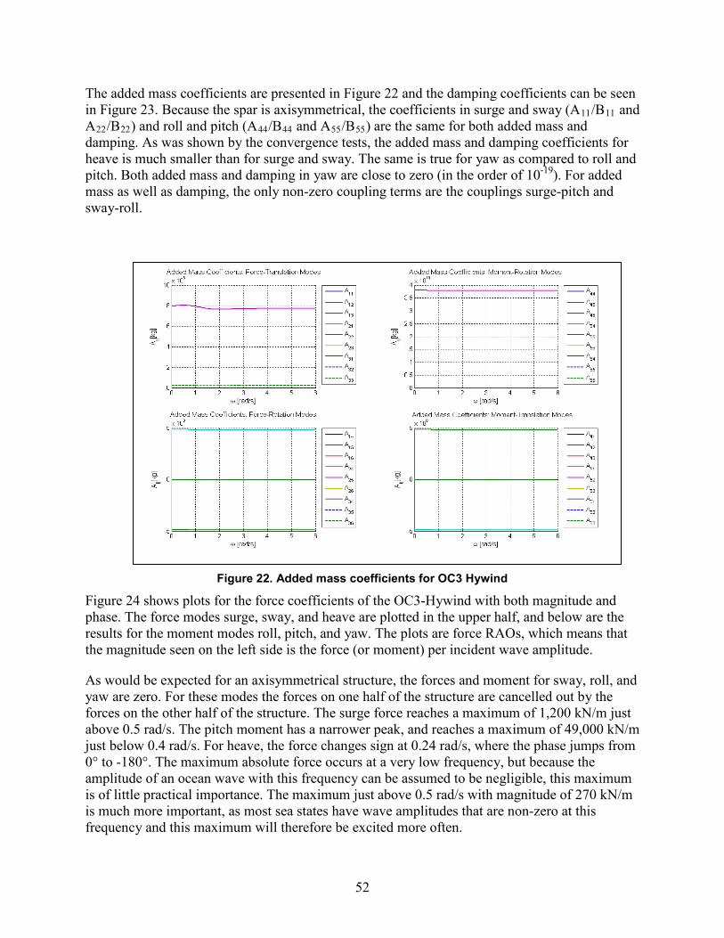
52
The added mass coefficients are presented in Figure 22 and the damping coefficients can be seen in Figure 23. Because the spar is axisymmetrical, the coefficients in surge and sway (A11/B11 and A22/B22) and roll and pitch (A44/B44 and A55/B55) are the same for both added mass and damping. As was shown by the convergence tests, the added mass and damping coefficients for heave is much smaller than for surge and sway. The same is true for yaw as compared to roll and pitch. Both added mass and damping in yaw are close to zero (in the order of 10-19). For added mass as well as damping, the only non-zero coupling terms are the couplings surge-pitch and sway-roll.
Figure 22. Added mass coefficients for OC3 Hywind
Figure 24 shows plots for the force coefficients of the OC3-Hywind with both magnitude and phase. The force modes surge, sway, and heave are plotted in the upper half, and below are the results for the moment modes roll, pitch, and yaw. The plots are force RAOs, which means that the magnitude seen on the left side is the force (or moment) per incident wave amplitude.
As would be expected for an axisymmetrical structure, the forces and moment for sway, roll, and yaw are zero. For these modes the forces on one half of the structure are cancelled out by the forces on the other half of the structure. The surge force reaches a maximum of 1,200 kN/m just above 0.5 rad/s. The pitch moment has a narrower peak, and reaches a maximum of 49,000 kN/m just below 0.4 rad/s. For heave, the force changes sign at 0.24 rad/s, where the phase jumps from 0° to -180°. The maximum absolute force occurs at a very low frequency, but because the amplitude of an ocean wave with this frequency can be assumed to be negligible, this maximum is of little practical importance. The maximum just above 0.5 rad/s with magnitude of 270 kN/m is much more important, as most sea states have wave amplitudes that are non-zero at this frequency and this maximum will therefore be excited more often.
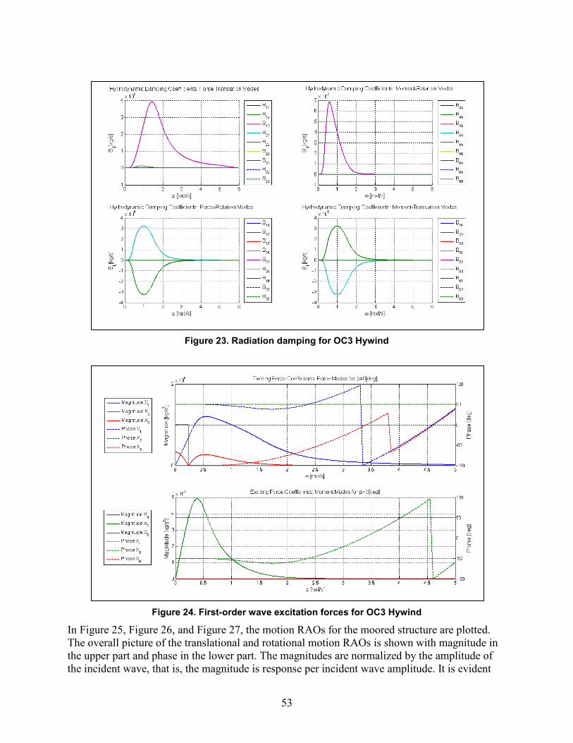
53
Figure 23. Radiation damping for OC3 Hywind
Figure 24. First-order wave excitation forces for OC3 Hywind
In Figure 25, Figure 26, and Figure 27, the motion RAOs for the moored structure are plotted. The overall picture of the translational and rotational motion RAOs is shown with magnitude in the upper part and phase in the lower part. The magnitudes are normalized by the amplitude of the incident wave, that is, the magnitude is response per incident wave amplitude. It is evident
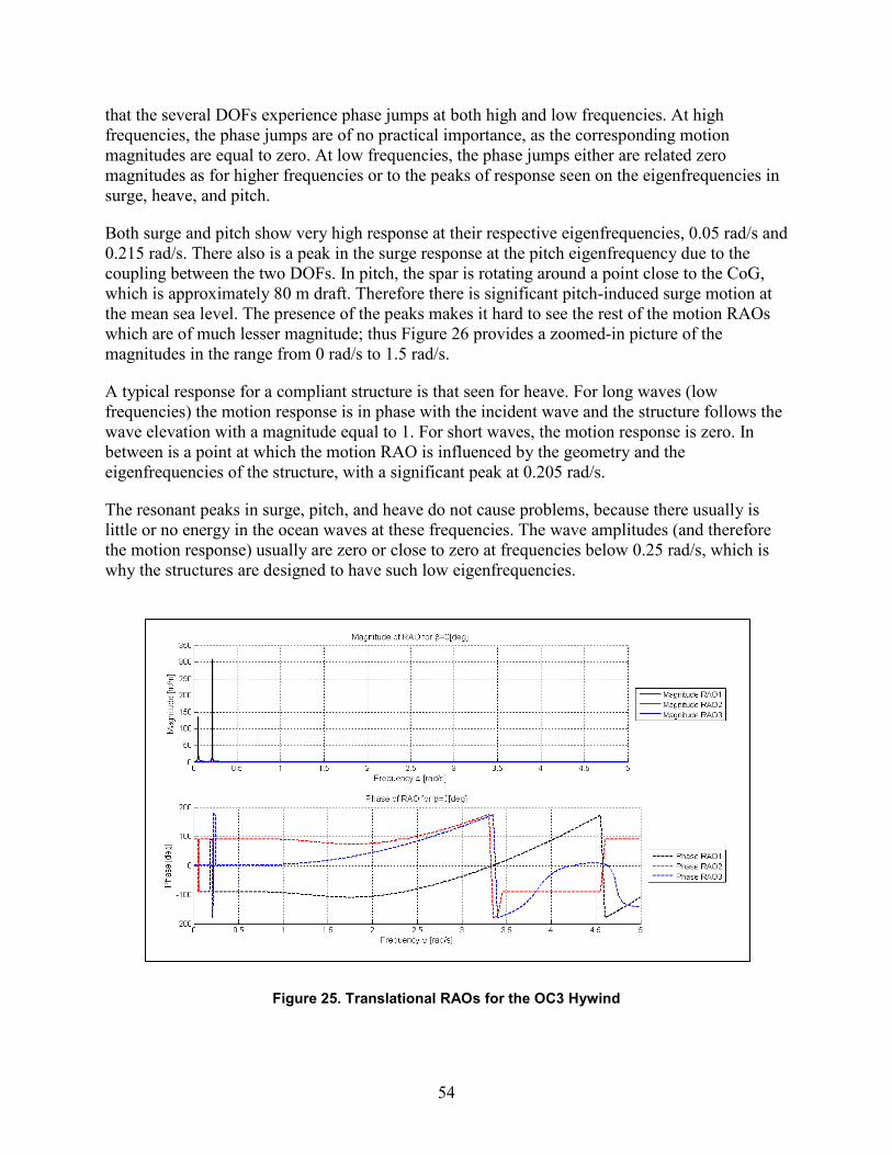
54
that the several DOFs experience phase jumps at both high and low frequencies. At high frequencies, the phase jumps are of no practical importance, as the corresponding motion magnitudes are equal to zero. At low frequencies, the phase jumps either are related zero magnitudes as for higher frequencies or to the peaks of response seen on the eigenfrequencies in surge, heave, and pitch.
Both surge and pitch show very high response at their respective eigenfrequencies, 0.05 rad/s and 0.215 rad/s. There also is a peak in the surge response at the pitch eigenfrequency due to the coupling between the two DOFs. In pitch, the spar is rotating around a point close to the CoG, which is approximately 80 m draft. Therefore there is significant pitch-induced surge motion at the mean sea level. The presence of the peaks makes it hard to see the rest of the motion RAOs which are of much lesser magnitude; thus Figure 26 provides a zoomed-in picture of the magnitudes in the range from 0 rad/s to 1.5 rad/s.
A typical response for a compliant structure is that seen for heave. For long waves (low frequencies) the motion response is in phase with the incident wave and the structure follows the wave elevation with a magnitude equal to 1. For short waves, the motion response is zero. In between is a point at which the motion RAO is influenced by the geometry and the eigenfrequencies of the structure, with a significant peak at 0.205 rad/s.
The resonant peaks in surge, pitch, and heave do not cause problems, because there usually is little or no energy in the ocean waves at these frequencies. The wave amplitudes (and therefore the motion response) usually are zero or close to zero at frequencies below 0.25 rad/s, which is why the structures are designed to have such low eigenfrequencies.
Figure 25. Translational RAOs for the OC3 Hywind
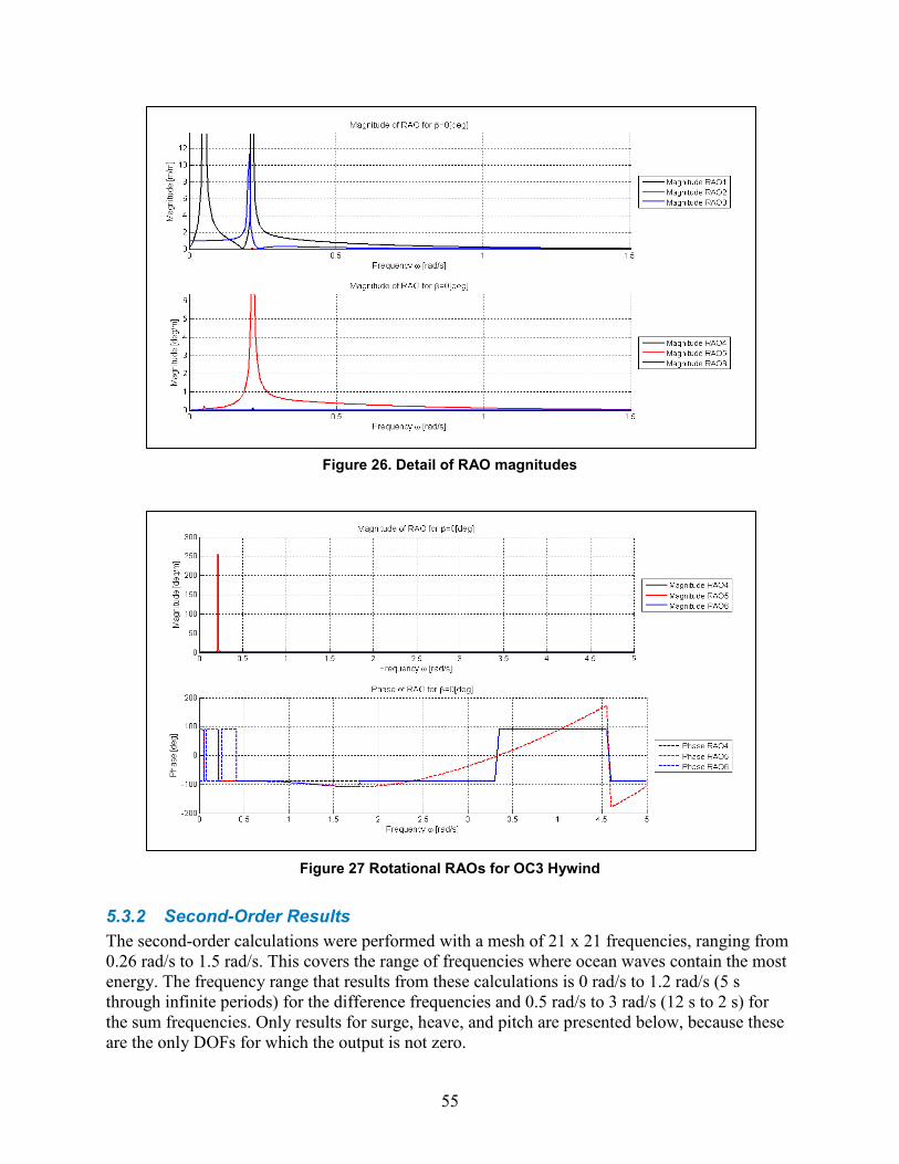
55
Figure 26. Detail of RAO magnitudes
Figure 27 Rotational RAOs for OC3 Hywind
5.3.2 Second-Order Results The second-order calculations were performed with a mesh of 21 x 21 frequencies, ranging from 0.26 rad/s to 1.5 rad/s. This covers the range of frequencies where ocean waves contain the most energy. The frequency range that results from these calculations is 0 rad/s to 1.2 rad/s (5 s through infinite periods) for the difference frequencies and 0.5 rad/s to 3 rad/s (12 s to 2 s) for the sum frequencies. Only results for surge, heave, and pitch are presented below, because these are the only DOFs for which the output is not zero.
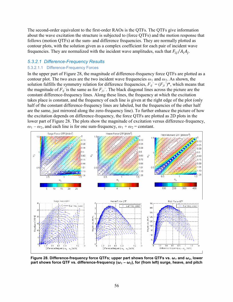
56
The second-order equivalent to the first-order RAOs is the QTFs. The QTFs give information about the wave excitation the structure is subjected to (force QTFs) and the motion response that follows (motion QTFs) at the sum- and difference frequencies. They are normally plotted as contour plots, with the solution given as a complex coefficient for each pair of incident wave frequencies. They are normalized with the incident wave amplitudes, such that 𝐹𝑖𝑗 𝐴𝑖𝐴𝑗⁄ .
5.3.2.1 Difference-Frequency Results 5.3.2.1.1 Difference-Frequency Forces In the upper part of Figure 28, the magnitude of difference-frequency force QTFs are plotted as a contour plot. The two axes are the two incident wave frequencies ω1 and ω2. As shown, the solution fulfills the symmetry relation for difference frequencies, Fij
– = (Fji–)*, which means that
the magnitude of Fij–is the same as for Fj i
–. The black diagonal lines across the picture are the constant difference-frequency lines. Along these lines, the frequency at which the excitation takes place is constant, and the frequency of each line is given at the right edge of the plot (only half of the constant difference-frequency lines are labeled, but the frequencies of the other half are the same, just mirrored along the zero-frequency line). To further enhance the picture of how the excitation depends on difference-frequency, the force QTFs are plotted as 2D plots in the lower part of Figure 28. The plots show the magnitude of excitation versus difference-frequency, ω1 – ω2, and each line is for one sum-frequency, ω1 + ω2 = constant.
Figure 28. Difference-frequency force QTFs; upper part shows force QTFs vs. ω1 and ω2, lower part shows force QTF vs. difference-frequency (ω1 – ω2), for (from left) surge, heave, and pitch
57
The peak of the excitation in surge is found at high incident-wave frequencies in the middle of the difference-frequency range. The greatest value is approximately 27 kN/m2. The difference-frequency at which the peak excitation occurs for heave is about 0.4 rad/s, with a value of 7 kN/m2. The pitch force QTF show much of the same behavior as the heave QTF, with a consistent peak at about 0.45 rad/s, and a peak value of 42 kNm/m2.
The force results only are provided for a restrained configuration, namely that including a mooring system. Because the second-order solution depends on the first-order motions, the second-order forces with and without mooring system differ slightly. In the case of the spar, however, the difference is so minimal that it is not considered necessary to show the results from both configurations.
The second-order motion QTF clearly is of smaller magnitude than the first-order RAOs. Keep in mind, however, that QTFs are normalized with the incident wave amplitude squared. This increases the difference between the first- and second-order RAOs if the waves are small, but increases the relative importance of the second-order parts if the waves are high. Also, the total response at one difference-frequency is the sum of contributions from several pairs of incident waves. For this sum is to be correct, however, all of the (complex) coefficients in the QTF first must be multiplied by the complex amplitudes of the incident waves. The incident wave amplitudes only are available after a certain sea state with certain random phases is selected. Section 5.4, provides an example and compares the second-order forces and motions to first-order forces and motions in specific sea states.
5.3.2.1.2 Difference-Frequency Motions—With and Without Mooring Systems The motion RAOs are shown for both a freely floating platform (not including mooring system stiffness) in Figure 29, and for a moored platform (including mooring system stiffness from FAST linearization) in Figure 30.
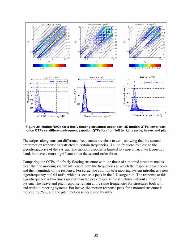
58
Figure 29. Motion RAOs for a freely floating structure; upper part: 3D motion QTFs, lower part: motion QTFs vs. difference-frequency motion QTFs for (from left to right) surge, heave, and pitch
The stripes along constant difference-frequencies are close to zero, showing that the second-order motion response is restricted to certain frequencies, i.e., to frequencies close to the eigenfrequencies of the system. The motion response is limited to a much narrower frequency band, but have a more significant value the second-order forces.
Comparing the QTFs of a freely floating structure with the those of a moored structure makes clear that the mooring system influences both the frequencies at which the response peak occurs and the magnitude of the response. For surge, the addition of a mooring system introduces a new eigenfrequency at 0.05 rad/s, which is seen as a peak in the 2-D surge plot. The response at this eigenfrequency is two times greater than the peak response for structures without a mooring system. The heave and pitch response remain at the same frequencies for structures both with and without mooring systems. For heave, the motion response peak for a moored structure is reduced by 25%, and the pitch motion is decreased by 40%.
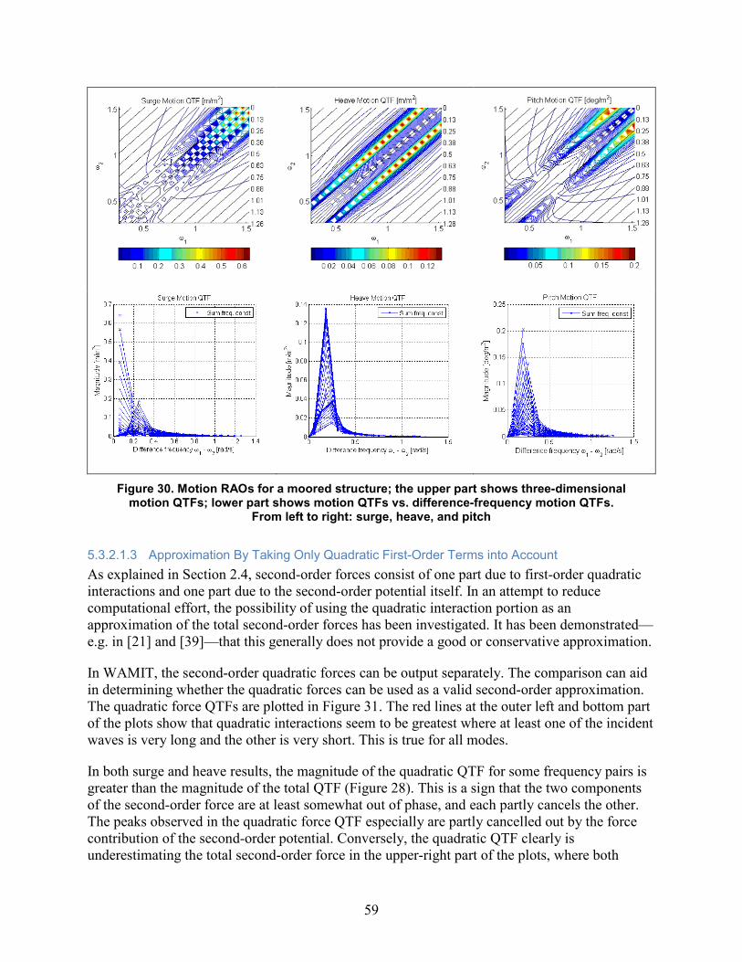
59
Figure 30. Motion RAOs for a moored structure; the upper part shows three-dimensional motion QTFs; lower part shows motion QTFs vs. difference-frequency motion QTFs.
From left to right: surge, heave, and pitch
5.3.2.1.3 Approximation By Taking Only Quadratic First-Order Terms into Account As explained in Section 2.4, second-order forces consist of one part due to first-order quadratic interactions and one part due to the second-order potential itself. In an attempt to reduce computational effort, the possibility of using the quadratic interaction portion as an approximation of the total second-order forces has been investigated. It has been demonstrated—e.g. in [21] and [39]—that this generally does not provide a good or conservative approximation.
In WAMIT, the second-order quadratic forces can be output separately. The comparison can aid in determining whether the quadratic forces can be used as a valid second-order approximation. The quadratic force QTFs are plotted in Figure 31. The red lines at the outer left and bottom part of the plots show that quadratic interactions seem to be greatest where at least one of the incident waves is very long and the other is very short. This is true for all modes.
In both surge and heave results, the magnitude of the quadratic QTF for some frequency pairs is greater than the magnitude of the total QTF (Figure 28). This is a sign that the two components of the second-order force are at least somewhat out of phase, and each partly cancels the other. The peaks observed in the quadratic force QTF especially are partly cancelled out by the force contribution of the second-order potential. Conversely, the quadratic QTF clearly is underestimating the total second-order force in the upper-right part of the plots, where both
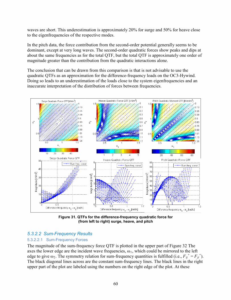
60
waves are short. This underestimation is approximately 20% for surge and 50% for heave close to the eigenfrequencies of the respective modes.
In the pitch data, the force contribution from the second-order potential generally seems to be dominant, except at very long waves. The second-order quadratic forces show peaks and dips at about the same frequencies as for the total QTF, but the total QTF is approximately one order of magnitude greater than the contribution from the quadratic interactions alone.
The conclusion that can be drawn from this comparison is that is not advisable to use the quadratic QTFs as an approximation for the difference-frequency loads on the OC3-Hywind. Doing so leads to an underestimation of the loads close to the system eigenfrequencies and an inaccurate interpretation of the distribution of forces between frequencies.
Figure 31. QTFs for the difference-frequency quadratic force for (from left to right) surge, heave, and pitch
5.3.2.2 Sum-Frequency Results 5.3.2.2.1 Sum-Frequency Forces The magnitude of the sum-frequency force QTF is plotted in the upper part of Figure 32 The axes the lower edge are the incident wave frequencies, ω1, which could be mirrored to the left edge to give ω2. The symmetry relation for sum-frequency quantities is fulfilled (i.e., Fij
+ = Fji+).
The black diagonal lines across are the constant sum-frequency lines. The black lines in the right upper part of the plot are labeled using the numbers on the right edge of the plot. At these
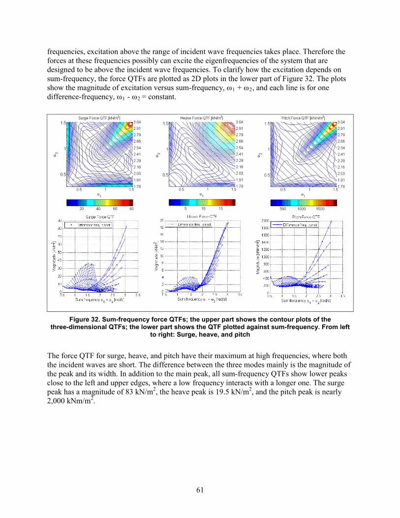
61
frequencies, excitation above the range of incident wave frequencies takes place. Therefore the forces at these frequencies possibly can excite the eigenfrequencies of the system that are designed to be above the incident wave frequencies. To clarify how the excitation depends on sum-frequency, the force QTFs are plotted as 2D plots in the lower part of Figure 32. The plots show the magnitude of excitation versus sum-frequency, ω1 + ω2, and each line is for one difference-frequency, ω1 - ω2 = constant.
Figure 32. Sum-frequency force QTFs; the upper part shows the contour plots of the three-dimensional QTFs; the lower part shows the QTF plotted against sum-frequency. From left
to right: Surge, heave, and pitch
The force QTF for surge, heave, and pitch have their maximum at high frequencies, where both the incident waves are short. The difference between the three modes mainly is the magnitude of the peak and its width. In addition to the main peak, all sum-frequency QTFs show lower peaks close to the left and upper edges, where a low frequency interacts with a longer one. The surge peak has a magnitude of 83 kN/m2, the heave peak is 19.5 kN/m2, and the pitch peak is nearly 2,000 kNm/m2.
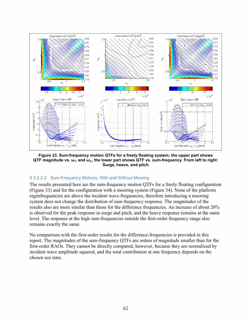
62
Figure 33. Sum-frequency motion QTFs for a freely floating system; the upper part shows QTF magnitude vs. ω1 and ω2, the lower part shows QTF vs. sum-frequency. From left to right:
Surge, heave, and pitch
5.3.2.2.2 Sum-Frequency Motions, With and Without Mooring The results presented here are the sum-frequency motion QTFs for a freely floating configuration (Figure 33) and for the configuration with a mooring system (Figure 34). None of the platform eigenfrequencies are above the incident wave frequencies, therefore introducing a mooring system does not change the distribution of sum-frequency response. The magnitudes of the results also are more similar than those for the difference frequencies. An increase of about 20% is observed for the peak response in surge and pitch, and the heave response remains at the same level. The response at the high sum-frequencies outside the first-order frequency range also remains exactly the same.
No comparison with the first-order results for the difference-frequencies is provided in this report. The magnitudes of the sum-frequency QTFs are orders of magnitude smaller than for the first-order RAOs. They cannot be directly compared, however, because they are normalized by incident wave amplitude squared, and the total contribution at one frequency depends on the chosen sea state.
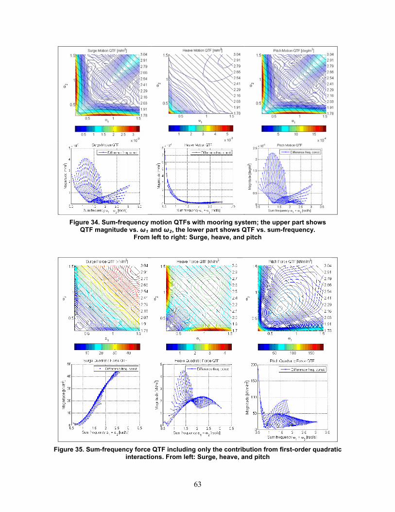
63
Figure 34. Sum-frequency motion QTFs with mooring system; the upper part shows QTF magnitude vs. ω1 and ω2, the lower part shows QTF vs. sum-frequency.
From left to right: Surge, heave, and pitch
Figure 35. Sum-frequency force QTF including only the contribution from first-order quadratic
interactions. From left: Surge, heave, and pitch
64
5.3.2.2.3 Approximation by First-Order Interactions The sum-frequency quadratic force QTF is shown in Figure 35. This is the component of the sum-frequency force that is due to quadratic interactions of first-order terms, and does not include the contribution from the second-order potential.
A comparison of the quadratic QTF to the total QTF in Figure 32 reveals significant differences. For surge, the quadratic QTF is almost constant for a given sum-frequency, although the total QTF shows a peak where both incident waves have equal frequency. The peak also is under-estimated by about 50%. For heave, the quadratic QTF seems to be a decent approximation for low sum-frequencies (in the lower right part of the plot), and the peak of the total force QTF at high sum-frequencies is underestimated by an order of magnitude. The quadratic force QTF for pitch seems to underestimate the peak of the total force QTF by almost two orders of magnitude, and the lower sum-frequencies are better represented by the quadratic force QTF. This is consistent with what was found by the investigation of the second-order loads on a slender cylinder in [39]. The study states that “at low frequencies (long waves), the QTF is well represented by the quadratic part, while at higher frequencies the contribution from the second-order potential is dominating.”
We conclude that the quadratic QTF is not a good approximation for the total sum-frequency forces for the OC3-Hywind.
5.4 Comparison of First-Order Response and Second-Order Response in Different Sea States
The first-order force and motion RAOs and the second-order force and motion QTFs are normalized results that provide the complex force and motion amplitudes in regular waves of unit amplitude. To obtain the force or motion experienced by the platform in the ocean, where the waves no longer are of unit amplitude, the coefficients must be multiplied by the complex amplitude of the incident waves. Examples are provided by Equation 2–57 for first-order quantities and by Equation 2–74 for second-order quantities.
The first-order quantities depend on only a single incident wave, whereas the second-order quantities depend on pairs of incident waves. This means that the first-order quantities are normalized by one wave amplitude and the second-order quantities by two wave amplitudes. Consequently, direct comparison of first- and second-order quantities only is possible after a sea state is chosen and the forces and motions can be computed for the given wave amplitudes.
The complex wave amplitude A = aeiφ is given by an amplitude 𝑎 and a random phase φ. For the waves used here, the amplitudes at frequency ω are determined directly and uniquely from the wave spectrum S(ω), without any randomness included (as normally is included in FAST). The wave spectrum is a Pierson-Moscowitz spectrum.
The comparison between first-order and second-order results is composed of two different parts. In the first part, the first-order RAOs and the second-order QTFs simply are multiplied by the wave spectrum of a given sea state to get the force and motion response induced by each individual wave and by each wave pair. In the second part, all wave pairs that lead to the same sum-frequency or difference-frequency are summed to assess the overall sum-frequency and difference-frequency contributions to the force and motion response.
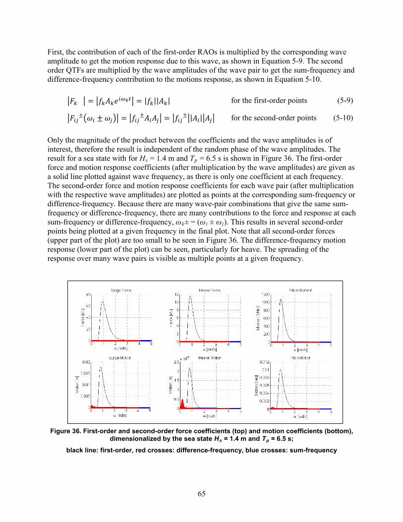
65
First, the contribution of each of the first-order RAOs is multiplied by the corresponding wave amplitude to get the motion response due to this wave, as shown in Equation 5-9. The second order QTFs are multiplied by the wave amplitudes of the wave pair to get the sum-frequency and difference-frequency contribution to the motions response, as shown in Equation 5-10.
�𝐹𝑘 � = �𝑓𝑘𝐴𝑘𝑒𝑖𝜔𝑘𝑡� = |𝑓𝑘||𝐴𝑘| for the first-order points (5-9)
�𝐹𝑖𝑗±�𝜔𝑖 ± 𝜔𝑗�� = �𝑓𝑖𝑗±𝐴𝑖𝐴𝑗� = �𝑓𝑖𝑗
±�|𝐴𝑖|�𝐴𝑗� for the second-order points (5-10)
Only the magnitude of the product between the coefficients and the wave amplitudes is of interest, therefore the result is independent of the random phase of the wave amplitudes. The result for a sea state with for Hs = 1.4 m and Tp = 6.5 s is shown in Figure 36. The first-order force and motion response coefficients (after multiplication by the wave amplitudes) are given as a solid line plotted against wave frequency, as there is only one coefficient at each frequency. The second-order force and motion response coefficients for each wave pair (after multiplication with the respective wave amplitudes) are plotted as points at the corresponding sum-frequency or difference-frequency. Because there are many wave-pair combinations that give the same sum-frequency or difference-frequency, there are many contributions to the force and response at each sum-frequency or difference-frequency, ωk± = (ωi ± ωj). This results in several second-order points being plotted at a given frequency in the final plot. Note that all second-order forces (upper part of the plot) are too small to be seen in Figure 36. The difference-frequency motion response (lower part of the plot) can be seen, particularly for heave. The spreading of the response over many wave pairs is visible as multiple points at a given frequency.
Figure 36. First-order and second-order force coefficients (top) and motion coefficients (bottom), dimensionalized by the sea state Hs = 1.4 m and Tp = 6.5 s;
black line: first-order, red crosses: difference-frequency, blue crosses: sum-frequency
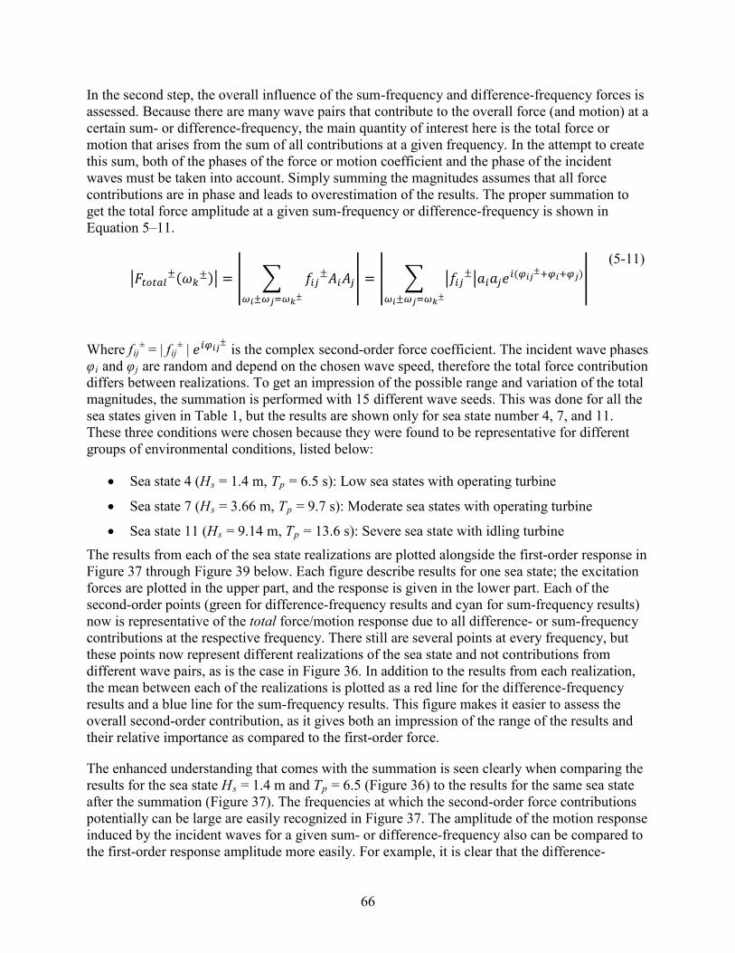
66
In the second step, the overall influence of the sum-frequency and difference-frequency forces is assessed. Because there are many wave pairs that contribute to the overall force (and motion) at a certain sum- or difference-frequency, the main quantity of interest here is the total force or motion that arises from the sum of all contributions at a given frequency. In the attempt to create this sum, both of the phases of the force or motion coefficient and the phase of the incident waves must be taken into account. Simply summing the magnitudes assumes that all force contributions are in phase and leads to overestimation of the results. The proper summation to get the total force amplitude at a given sum-frequency or difference-frequency is shown in Equation 5–11.
�𝐹𝑡𝑜𝑡𝑎𝑙±(𝜔𝑘±)� = � � 𝑓𝑖𝑗
±𝐴𝑖𝐴𝑗𝜔𝑖±𝜔𝑗=𝜔𝑘±
� = � � �𝑓𝑖𝑗±�𝑎𝑖𝑎𝑗𝑒𝑖(𝜑𝑖𝑗
±+𝜑𝑖+𝜑𝑗)
𝜔𝑖±𝜔𝑗=𝜔𝑘±
�
(5-11)
Where fij± = | fij
± | 𝑒𝑖𝜑𝑖𝑗± is the complex second-order force coefficient. The incident wave phases
φi and φj are random and depend on the chosen wave speed, therefore the total force contribution differs between realizations. To get an impression of the possible range and variation of the total magnitudes, the summation is performed with 15 different wave seeds. This was done for all the sea states given in Table 1, but the results are shown only for sea state number 4, 7, and 11. These three conditions were chosen because they were found to be representative for different groups of environmental conditions, listed below:
• Sea state 4 (Hs = 1.4 m, Tp = 6.5 s): Low sea states with operating turbine
• Sea state 7 (Hs = 3.66 m, Tp = 9.7 s): Moderate sea states with operating turbine
• Sea state 11 (Hs = 9.14 m, Tp = 13.6 s): Severe sea state with idling turbine The results from each of the sea state realizations are plotted alongside the first-order response in
Figure 37 through Figure 39 below. Each figure describe results for one sea state; the excitation forces are plotted in the upper part, and the response is given in the lower part. Each of the second-order points (green for difference-frequency results and cyan for sum-frequency results) now is representative of the total force/motion response due to all difference- or sum-frequency contributions at the respective frequency. There still are several points at every frequency, but these points now represent different realizations of the sea state and not contributions from different wave pairs, as is the case in Figure 36. In addition to the results from each realization, the mean between each of the realizations is plotted as a red line for the difference-frequency results and a blue line for the sum-frequency results. This figure makes it easier to assess the overall second-order contribution, as it gives both an impression of the range of the results and their relative importance as compared to the first-order force.
The enhanced understanding that comes with the summation is seen clearly when comparing the results for the sea state Hs = 1.4 m and Tp = 6.5 (Figure 36) to the results for the same sea state after the summation (Figure 37). The frequencies at which the second-order force contributions potentially can be large are easily recognized in Figure 37. The amplitude of the motion response induced by the incident waves for a given sum- or difference-frequency also can be compared to the first-order response amplitude more easily. For example, it is clear that the difference-
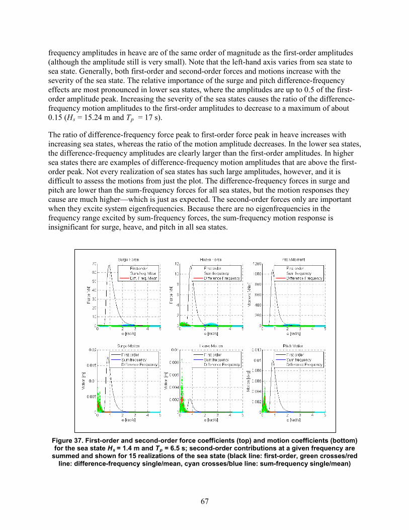
67
frequency amplitudes in heave are of the same order of magnitude as the first-order amplitudes (although the amplitude still is very small). Note that the left-hand axis varies from sea state to sea state. Generally, both first-order and second-order forces and motions increase with the severity of the sea state. The relative importance of the surge and pitch difference-frequency effects are most pronounced in lower sea states, where the amplitudes are up to 0.5 of the first-order amplitude peak. Increasing the severity of the sea states causes the ratio of the difference-frequency motion amplitudes to the first-order amplitudes to decrease to a maximum of about 0.15 (Hs = 15.24 m and Tp = 17 s).
The ratio of difference-frequency force peak to first-order force peak in heave increases with increasing sea states, whereas the ratio of the motion amplitude decreases. In the lower sea states, the difference-frequency amplitudes are clearly larger than the first-order amplitudes. In higher sea states there are examples of difference-frequency motion amplitudes that are above the first-order peak. Not every realization of sea states has such large amplitudes, however, and it is difficult to assess the motions from just the plot. The difference-frequency forces in surge and pitch are lower than the sum-frequency forces for all sea states, but the motion responses they cause are much higher—which is just as expected. The second-order forces only are important when they excite system eigenfrequencies. Because there are no eigenfrequencies in the frequency range excited by sum-frequency forces, the sum-frequency motion response is insignificant for surge, heave, and pitch in all sea states.
Figure 37. First-order and second-order force coefficients (top) and motion coefficients (bottom) for the sea state Hs = 1.4 m and Tp = 6.5 s; second-order contributions at a given frequency are
summed and shown for 15 realizations of the sea state (black line: first-order, green crosses/red line: difference-frequency single/mean, cyan crosses/blue line: sum-frequency single/mean)
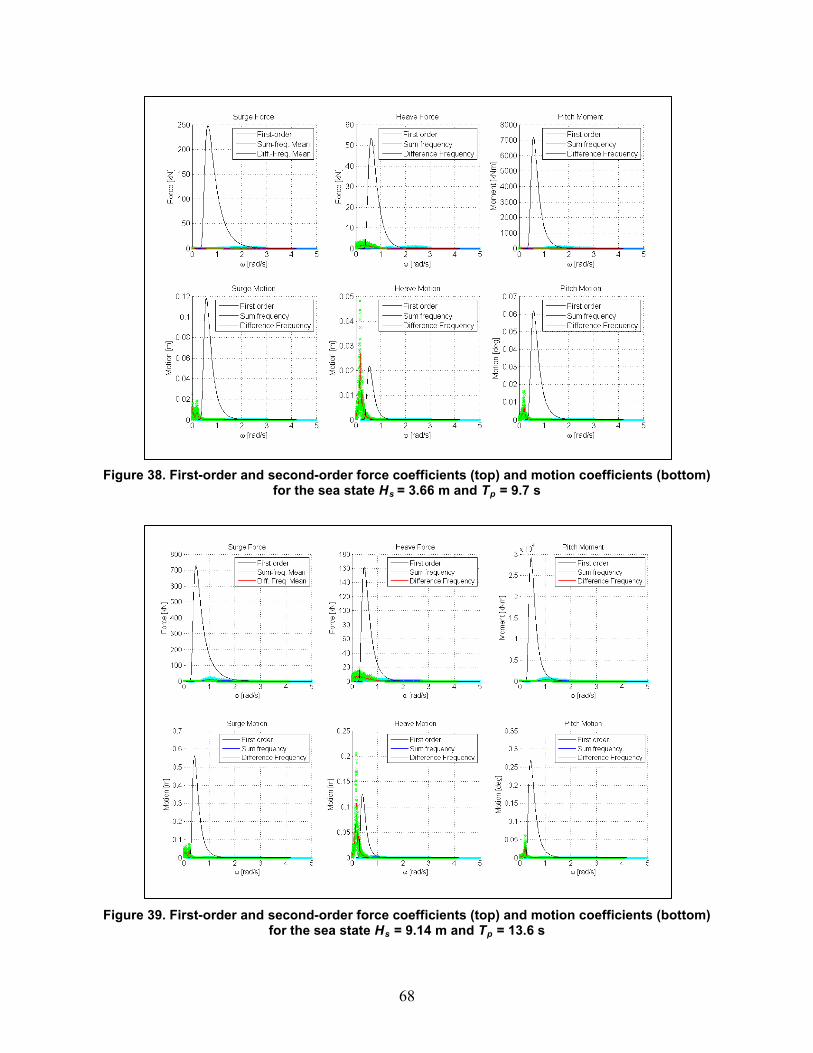
68
Figure 38. First-order and second-order force coefficients (top) and motion coefficients (bottom) for the sea state Hs = 3.66 m and Tp = 9.7 s
Figure 39. First-order and second-order force coefficients (top) and motion coefficients (bottom) for the sea state Hs = 9.14 m and Tp = 13.6 s
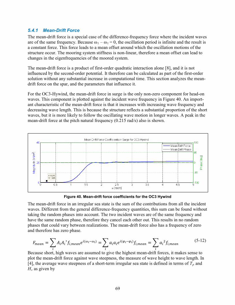
69
5.4.1 Mean-Drift Force The mean-drift force is a special case of the difference-frequency force where the incident waves are of the same frequency. Because ω1 – ω1 = 0, the oscillation period is infinite and the result is a constant force. This force leads to a mean offset around which the oscillation motions of the structure occur. The mooring system stiffness is non-linear, therefore a mean offset can lead to changes in the eigenfrequencies of the moored system.
The mean-drift force is a product of first-order quadratic interaction alone [8], and it is not influenced by the second-order potential. It therefore can be calculated as part of the first-order solution without any substantial increase in computational time. This section analyzes the mean-drift force on the spar, and the parameters that influence it.
For the OC3-Hywind, the mean-drift force in surge is the only non-zero component for head-on waves. This component is plotted against the incident wave frequency in Figure 40. An import-ant characteristic of the mean-drift force is that it increases with increasing wave frequency and decreasing wave length. This is because the structure reflects a substantial proportion of the short waves, but it is more likely to follow the oscillating wave motion in longer waves. A peak in the mean-drift force at the pitch natural frequency (0.215 rad/s) also is shown.
Figure 40. Mean-drift force coefficients for the OC3 Hywind
The mean-drift force in an irregular sea state is the sum of the contributions from all the incident waves. Different from the general difference-frequency quantities, this sum can be found without taking the random phases into account. The two incident waves are of the same frequency and have the same random phase, therefore they cancel each other out. This results in no random phases that could vary between realizations. The mean-drift force also has a frequency of zero and therefore has zero phase.
𝐹𝑚𝑒𝑎𝑛 = �𝐴𝑖𝐴𝑖∗𝑓𝑖,𝑚𝑒𝑎𝑛𝑒𝑖(𝜔𝑖−𝜔𝑖) =𝑖
�𝑎𝑖𝑎𝑖𝑒𝑖(𝜑𝑖−𝜑𝑖)𝑓𝑖,𝑚𝑒𝑎𝑛 = �𝑎𝑖2𝑓𝑖,𝑚𝑒𝑎𝑛𝑖𝑖
(5-12)
Because short, high waves are assumed to give the highest mean-drift forces, it makes sense to plot the mean-drift force against wave steepness, the measure of wave height to wave length. In [4], the average wave steepness of a short-term irregular sea state is defined in terms of Tp and Hs as given by
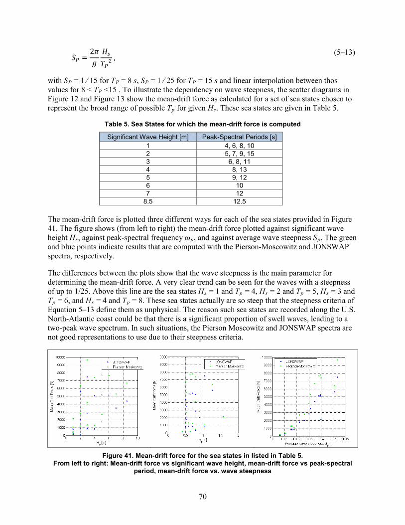
70
𝑆𝑃 =2𝜋𝑔
𝐻𝑠𝑇𝑃2
, (5–13)
with SP = 1 ⁄ 15 for TP = 8 s, SP = 1 ⁄ 25 for TP = 15 s and linear interpolation between thos values for 8 < TP <15 . To illustrate the dependency on wave steepness, the scatter diagrams in Figure 12 and Figure 13 show the mean-drift force as calculated for a set of sea states chosen to represent the broad range of possible Tp for given Hs. These sea states are given in Table 5.
Table 5. Sea States for which the mean-drift force is computed
Significant Wave Height [m] Peak-Spectral Periods [s] 1 4, 6, 8, 10 2 5, 7, 9, 15 3 6, 8, 11 4 8, 13 5 9, 12 6 10 7 12
8.5 12.5 The mean-drift force is plotted three different ways for each of the sea states provided in Figure 41. The figure shows (from left to right) the mean-drift force plotted against significant wave height Hs, against peak-spectral frequency ωp, and against average wave steepness Sp. The green and blue points indicate results that are computed with the Pierson-Moscowitz and JONSWAP spectra, respectively.
The differences between the plots show that the wave steepness is the main parameter for determining the mean-drift force. A very clear trend can be seen for the waves with a steepness of up to 1/25. Above this line are the sea states Hs = 1 and Tp = 4, Hs = 2 and Tp = 5, Hs = 3 and Tp = 6, and Hs = 4 and Tp = 8. These sea states actually are so steep that the steepness criteria of Equation 5–13 define them as unphysical. The reason such sea states are recorded along the U.S. North-Atlantic coast could be that there is a significant proportion of swell waves, leading to a two-peak wave spectrum. In such situations, the Pierson Moscowitz and JONSWAP spectra are not good representations to use due to their steepness criteria.
Figure 41. Mean-drift force for the sea states in listed in Table 5.
From left to right: Mean-drift force vs significant wave height, mean-drift force vs peak-spectral period, mean-drift force vs. wave steepness
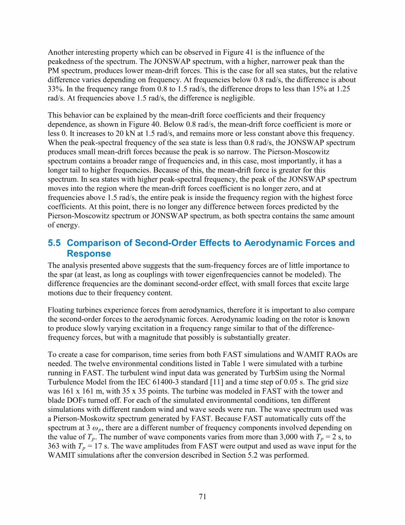
71
Another interesting property which can be observed in Figure 41 is the influence of the peakedness of the spectrum. The JONSWAP spectrum, with a higher, narrower peak than the PM spectrum, produces lower mean-drift forces. This is the case for all sea states, but the relative difference varies depending on frequency. At frequencies below 0.8 rad/s, the difference is about 33%. In the frequency range from 0.8 to 1.5 rad/s, the difference drops to less than 15% at 1.25 rad/s. At frequencies above 1.5 rad/s, the difference is negligible.
This behavior can be explained by the mean-drift force coefficients and their frequency dependence, as shown in Figure 40. Below 0.8 rad/s, the mean-drift force coefficient is more or less 0. It increases to 20 kN at 1.5 rad/s, and remains more or less constant above this frequency. When the peak-spectral frequency of the sea state is less than 0.8 rad/s, the JONSWAP spectrum produces small mean-drift forces because the peak is so narrow. The Pierson-Moscowitz spectrum contains a broader range of frequencies and, in this case, most importantly, it has a longer tail to higher frequencies. Because of this, the mean-drift force is greater for this spectrum. In sea states with higher peak-spectral frequency, the peak of the JONSWAP spectrum moves into the region where the mean-drift forces coefficient is no longer zero, and at frequencies above 1.5 rad/s, the entire peak is inside the frequency region with the highest force coefficients. At this point, there is no longer any difference between forces predicted by the Pierson-Moscowitz spectrum or JONSWAP spectrum, as both spectra contains the same amount of energy.
5.5 Comparison of Second-Order Effects to Aerodynamic Forces and Response
The analysis presented above suggests that the sum-frequency forces are of little importance to the spar (at least, as long as couplings with tower eigenfrequencies cannot be modeled). The difference frequencies are the dominant second-order effect, with small forces that excite large motions due to their frequency content.
Floating turbines experience forces from aerodynamics, therefore it is important to also compare the second-order forces to the aerodynamic forces. Aerodynamic loading on the rotor is known to produce slowly varying excitation in a frequency range similar to that of the difference-frequency forces, but with a magnitude that possibly is substantially greater.
To create a case for comparison, time series from both FAST simulations and WAMIT RAOs are needed. The twelve environmental conditions listed in Table 1 were simulated with a turbine running in FAST. The turbulent wind input data was generated by TurbSim using the Normal Turbulence Model from the IEC 61400-3 standard [11] and a time step of 0.05 s. The grid size was 161 x 161 m, with 35 x 35 points. The turbine was modeled in FAST with the tower and blade DOFs turned off. For each of the simulated environmental conditions, ten different simulations with different random wind and wave seeds were run. The wave spectrum used was a Pierson-Moskowitz spectrum generated by FAST. Because FAST automatically cuts off the spectrum at 3 ωp, there are a different number of frequency components involved depending on the value of Tp. The number of wave components varies from more than 3,000 with Tp = 2 s, to 363 with Tp = 17 s. The wave amplitudes from FAST were output and used as wave input for the WAMIT simulations after the conversion described in Section 5.2 was performed.
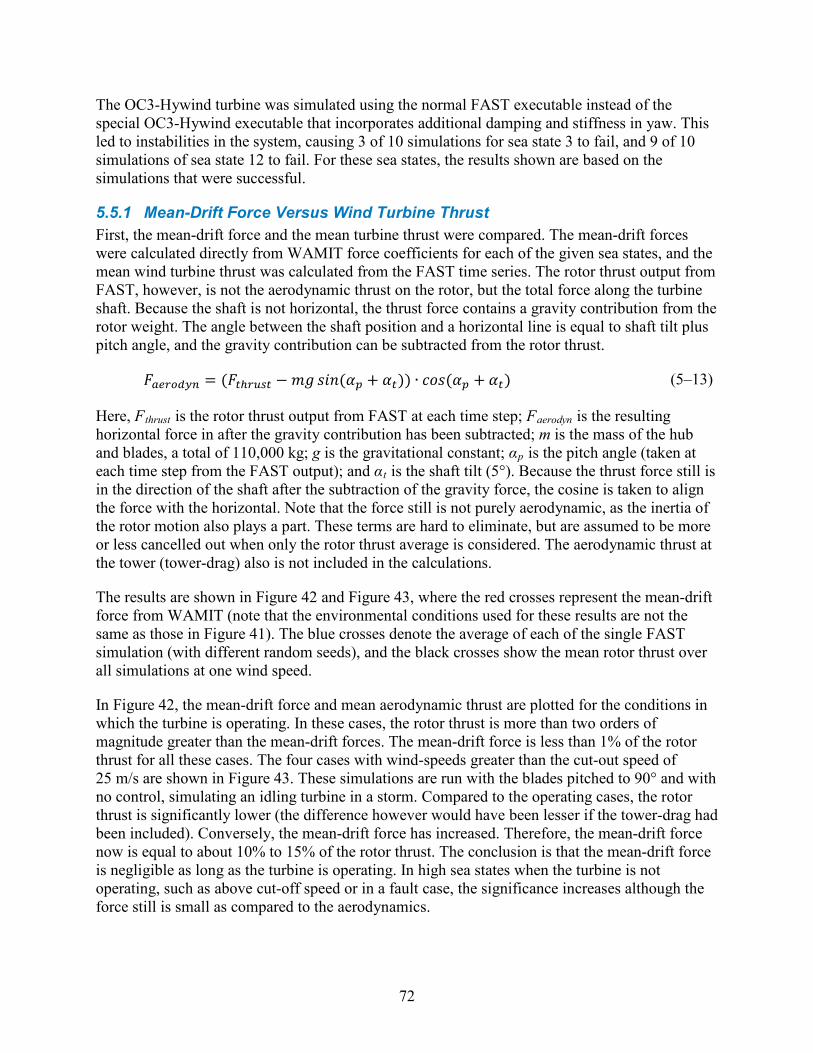
72
The OC3-Hywind turbine was simulated using the normal FAST executable instead of the special OC3-Hywind executable that incorporates additional damping and stiffness in yaw. This led to instabilities in the system, causing 3 of 10 simulations for sea state 3 to fail, and 9 of 10 simulations of sea state 12 to fail. For these sea states, the results shown are based on the simulations that were successful.
5.5.1 Mean-Drift Force Versus Wind Turbine Thrust First, the mean-drift force and the mean turbine thrust were compared. The mean-drift forces were calculated directly from WAMIT force coefficients for each of the given sea states, and the mean wind turbine thrust was calculated from the FAST time series. The rotor thrust output from FAST, however, is not the aerodynamic thrust on the rotor, but the total force along the turbine shaft. Because the shaft is not horizontal, the thrust force contains a gravity contribution from the rotor weight. The angle between the shaft position and a horizontal line is equal to shaft tilt plus pitch angle, and the gravity contribution can be subtracted from the rotor thrust.
𝐹𝑎𝑒𝑟𝑜𝑑𝑦𝑛 = (𝐹𝑡ℎ𝑟𝑢𝑠𝑡 − 𝑚𝑔 𝑠𝑖𝑛(𝛼𝑝 + 𝛼𝑡)) ∙ 𝑐𝑜𝑠 (𝛼𝑝 + 𝛼𝑡) (5–13)
Here, Fthrust is the rotor thrust output from FAST at each time step; Faerodyn is the resulting horizontal force in after the gravity contribution has been subtracted; m is the mass of the hub and blades, a total of 110,000 kg; g is the gravitational constant; αp is the pitch angle (taken at each time step from the FAST output); and αt is the shaft tilt (5°). Because the thrust force still is in the direction of the shaft after the subtraction of the gravity force, the cosine is taken to align the force with the horizontal. Note that the force still is not purely aerodynamic, as the inertia of the rotor motion also plays a part. These terms are hard to eliminate, but are assumed to be more or less cancelled out when only the rotor thrust average is considered. The aerodynamic thrust at the tower (tower-drag) also is not included in the calculations.
The results are shown in Figure 42 and Figure 43, where the red crosses represent the mean-drift force from WAMIT (note that the environmental conditions used for these results are not the same as those in Figure 41). The blue crosses denote the average of each of the single FAST simulation (with different random seeds), and the black crosses show the mean rotor thrust over all simulations at one wind speed.
In Figure 42, the mean-drift force and mean aerodynamic thrust are plotted for the conditions in which the turbine is operating. In these cases, the rotor thrust is more than two orders of magnitude greater than the mean-drift forces. The mean-drift force is less than 1% of the rotor thrust for all these cases. The four cases with wind-speeds greater than the cut-out speed of 25 m/s are shown in Figure 43. These simulations are run with the blades pitched to 90° and with no control, simulating an idling turbine in a storm. Compared to the operating cases, the rotor thrust is significantly lower (the difference however would have been lesser if the tower-drag had been included). Conversely, the mean-drift force has increased. Therefore, the mean-drift force now is equal to about 10% to 15% of the rotor thrust. The conclusion is that the mean-drift force is negligible as long as the turbine is operating. In high sea states when the turbine is not operating, such as above cut-off speed or in a fault case, the significance increases although the force still is small as compared to the aerodynamics.
73
5.5.2 Rotor Thrust: Excitation Frequencies To check the frequency content of the rotor thrust excitation, the time series from FAST were plotted as power spectral densities (PSDs) in Figure 44, Figure 45, and Figure 46. The forces were computed for all twelve environmental conditions in Table 1, but the results are shown only for sea states 4, 7, and 11. These results were found to be representative for different groups of environmental conditions:
• Sea state 4 (Hs = 1.44 m, Tp = 6.5 s): Low sea states with operating turbine
• Sea state 7 (Hs = 3.66 m, Tp = 9.7 s): Moderate sea states with operating turbine
• Sea state 11 (Hs = 9.14 m, Tp = 13.6 s): Severe sea state with idling turbine For the lower sea states, the excitation from rotor thrust at frequencies below the typical incident wave frequency range (0.25 – 1.5 rad/s) dominates. The high-frequency peaks are the harmonics of the rotor frequencies. The excitation also has a peak at about 0.21 rad/s, which is the pitch eigenfrequency. This pitch-frequency peak become more visible as the severity of the environmental condition grows. For the moderate sea state, a clear trend towards more excitation at the wave frequency is shown. The thrust excitation also increased, but no longer is as dominant as previously. In the highest sea states where the turbine no longer is operating, the low-frequency excitation drops by two orders of magnitude. The main rotor-thrust response is now in the wave-frequency domain, and at the pitch frequency.
The excitation both in the wave-frequency range and at the pitch frequency is due to turbine motions. When the turbine moves forward against the wind and then backward again because of the waves, the incident wind speed and hence the rotor thrust increases and decreases with the
Figure 42. Mean-drift force and mean wind turbine thrust in cases with operating turbine
Figure 43. Mean-drift force and mean turbine thrust in cases with idling turbine
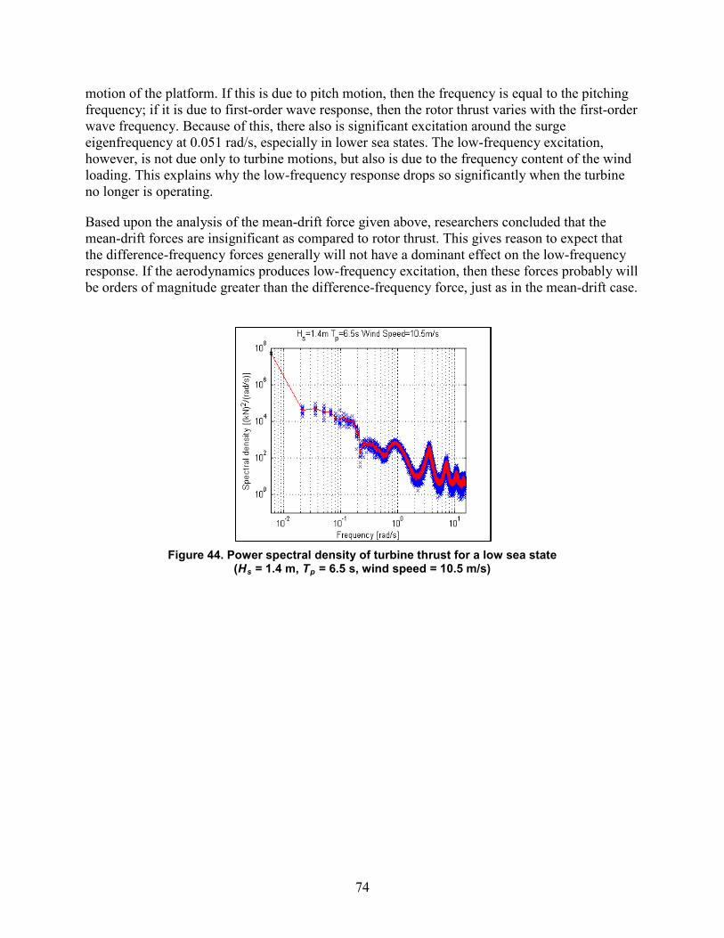
74
motion of the platform. If this is due to pitch motion, then the frequency is equal to the pitching frequency; if it is due to first-order wave response, then the rotor thrust varies with the first-order wave frequency. Because of this, there also is significant excitation around the surge eigenfrequency at 0.051 rad/s, especially in lower sea states. The low-frequency excitation, however, is not due only to turbine motions, but also is due to the frequency content of the wind loading. This explains why the low-frequency response drops so significantly when the turbine no longer is operating.
Based upon the analysis of the mean-drift force given above, researchers concluded that the mean-drift forces are insignificant as compared to rotor thrust. This gives reason to expect that the difference-frequency forces generally will not have a dominant effect on the low-frequency response. If the aerodynamics produces low-frequency excitation, then these forces probably will be orders of magnitude greater than the difference-frequency force, just as in the mean-drift case.
Figure 44. Power spectral density of turbine thrust for a low sea state (Hs = 1.4 m, Tp = 6.5 s, wind speed = 10.5 m/s)
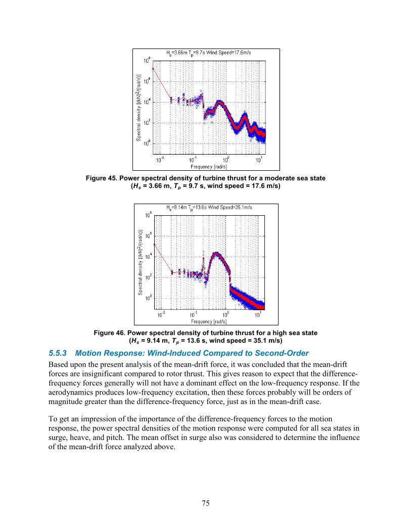
75
Figure 45. Power spectral density of turbine thrust for a moderate sea state (Hs = 3.66 m, Tp = 9.7 s, wind speed = 17.6 m/s)
Figure 46. Power spectral density of turbine thrust for a high sea state (Hs = 9.14 m, Tp = 13.6 s, wind speed = 35.1 m/s)
5.5.3 Motion Response: Wind-Induced Compared to Second-Order Based upon the present analysis of the mean-drift force, it was concluded that the mean-drift forces are insignificant compared to rotor thrust. This gives reason to expect that the difference-frequency forces generally will not have a dominant effect on the low-frequency response. If the aerodynamics produces low-frequency excitation, then these forces probably will be orders of magnitude greater than the difference-frequency force, just as in the mean-drift case.
To get an impression of the importance of the difference-frequency forces to the motion response, the power spectral densities of the motion response were computed for all sea states in surge, heave, and pitch. The mean offset in surge also was considered to determine the influence of the mean-drift force analyzed above.
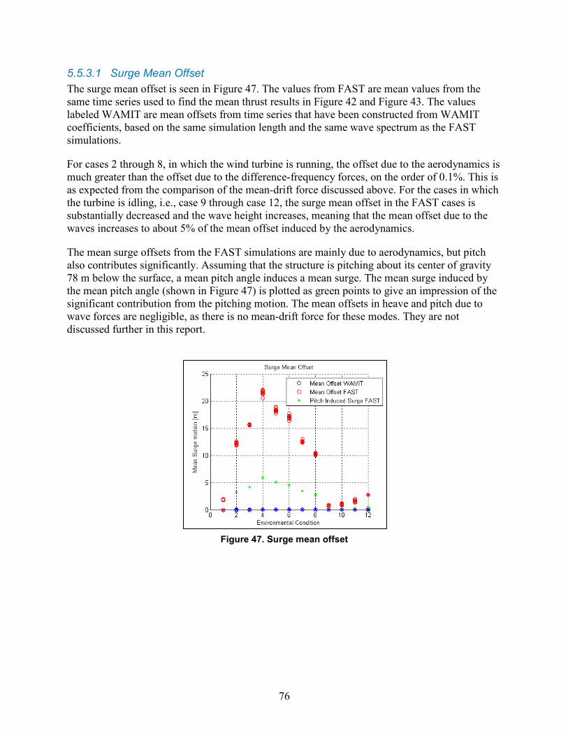
76
5.5.3.1 Surge Mean Offset The surge mean offset is seen in Figure 47. The values from FAST are mean values from the same time series used to find the mean thrust results in Figure 42 and Figure 43. The values labeled WAMIT are mean offsets from time series that have been constructed from WAMIT coefficients, based on the same simulation length and the same wave spectrum as the FAST simulations.
For cases 2 through 8, in which the wind turbine is running, the offset due to the aerodynamics is much greater than the offset due to the difference-frequency forces, on the order of 0.1%. This is as expected from the comparison of the mean-drift force discussed above. For the cases in which the turbine is idling, i.e., case 9 through case 12, the surge mean offset in the FAST cases is substantially decreased and the wave height increases, meaning that the mean offset due to the waves increases to about 5% of the mean offset induced by the aerodynamics.
The mean surge offsets from the FAST simulations are mainly due to aerodynamics, but pitch also contributes significantly. Assuming that the structure is pitching about its center of gravity 78 m below the surface, a mean pitch angle induces a mean surge. The mean surge induced by the mean pitch angle (shown in Figure 47) is plotted as green points to give an impression of the significant contribution from the pitching motion. The mean offsets in heave and pitch due to wave forces are negligible, as there is no mean-drift force for these modes. They are not discussed further in this report.
Figure 47. Surge mean offset
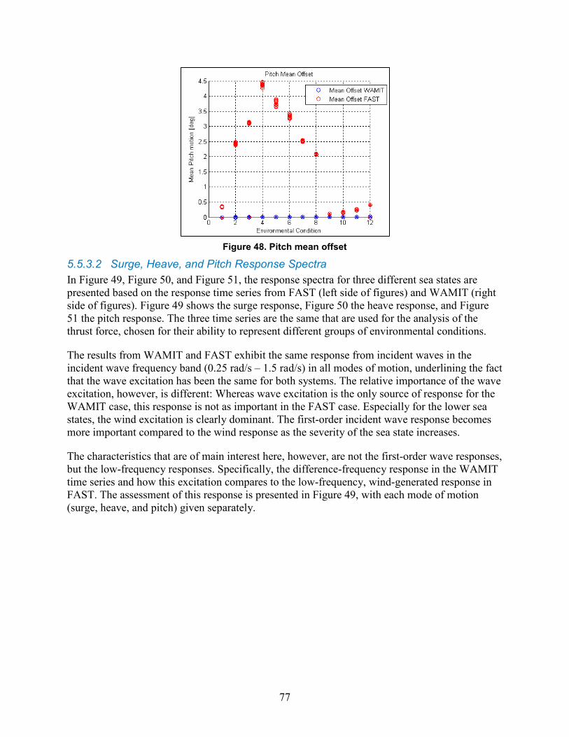
77
Figure 48. Pitch mean offset
5.5.3.2 Surge, Heave, and Pitch Response Spectra In Figure 49, Figure 50, and Figure 51, the response spectra for three different sea states are presented based on the response time series from FAST (left side of figures) and WAMIT (right side of figures). Figure 49 shows the surge response, Figure 50 the heave response, and Figure 51 the pitch response. The three time series are the same that are used for the analysis of the thrust force, chosen for their ability to represent different groups of environmental conditions.
The results from WAMIT and FAST exhibit the same response from incident waves in the incident wave frequency band (0.25 rad/s – 1.5 rad/s) in all modes of motion, underlining the fact that the wave excitation has been the same for both systems. The relative importance of the wave excitation, however, is different: Whereas wave excitation is the only source of response for the WAMIT case, this response is not as important in the FAST case. Especially for the lower sea states, the wind excitation is clearly dominant. The first-order incident wave response becomes more important compared to the wind response as the severity of the sea state increases.
The characteristics that are of main interest here, however, are not the first-order wave responses, but the low-frequency responses. Specifically, the difference-frequency response in the WAMIT time series and how this excitation compares to the low-frequency, wind-generated response in FAST. The assessment of this response is presented in Figure 49, with each mode of motion (surge, heave, and pitch) given separately.
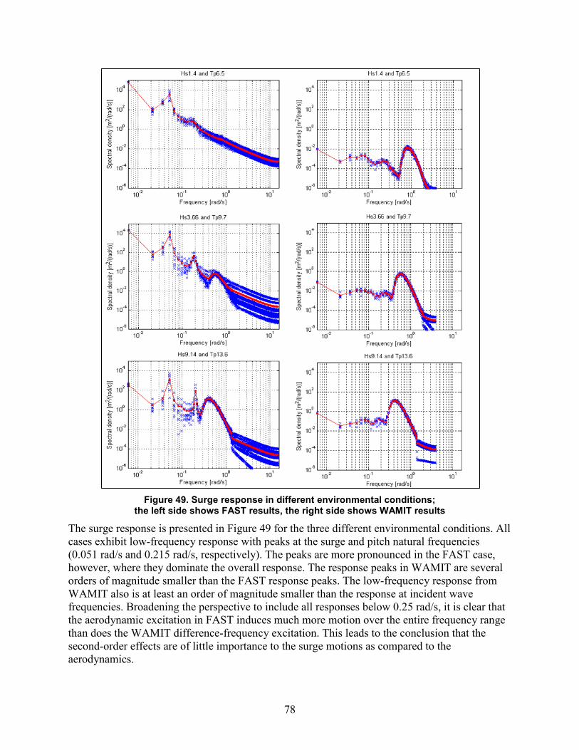
78
Figure 49. Surge response in different environmental conditions; the left side shows FAST results, the right side shows WAMIT results
The surge response is presented in Figure 49 for the three different environmental conditions. All cases exhibit low-frequency response with peaks at the surge and pitch natural frequencies (0.051 rad/s and 0.215 rad/s, respectively). The peaks are more pronounced in the FAST case, however, where they dominate the overall response. The response peaks in WAMIT are several orders of magnitude smaller than the FAST response peaks. The low-frequency response from WAMIT also is at least an order of magnitude smaller than the response at incident wave frequencies. Broadening the perspective to include all responses below 0.25 rad/s, it is clear that the aerodynamic excitation in FAST induces much more motion over the entire frequency range than does the WAMIT difference-frequency excitation. This leads to the conclusion that the second-order effects are of little importance to the surge motions as compared to the aerodynamics.
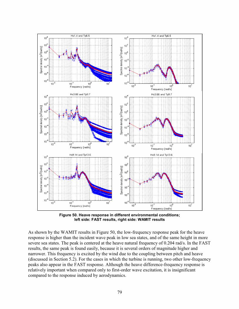
79
Figure 50. Heave response in different environmental conditions; left side: FAST results, right side: WAMIT results
As shown by the WAMIT results in Figure 50, the low-frequency response peak for the heave response is higher than the incident wave peak in low sea states, and of the same height in more severe sea states. The peak is centered at the heave natural frequency of 0.204 rad/s. In the FAST results, the same peak is found easily, because it is several orders of magnitude higher and narrower. This frequency is excited by the wind due to the coupling between pitch and heave (discussed in Section 5.2). For the cases in which the turbine is running, two other low-frequency peaks also appear in the FAST response. Although the heave difference-frequency response is relatively important when compared only to first-order wave excitation, it is insignificant compared to the response induced by aerodynamics.
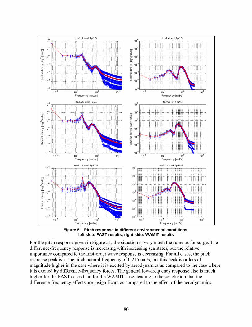
80
Figure 51. Pitch response in different environmental conditions; left side: FAST results, right side: WAMIT results
For the pitch response given in Figure 51, the situation is very much the same as for surge. The difference-frequency response is increasing with increasing sea states, but the relative importance compared to the first-order wave response is decreasing. For all cases, the pitch response peak is at the pitch natural frequency of 0.215 rad/s, but this peak is orders of magnitude higher in the case where it is excited by aerodynamics as compared to the case where it is excited by difference-frequency forces. The general low-frequency response also is much higher for the FAST cases than for the WAMIT case, leading to the conclusion that the difference-frequency effects are insignificant as compared to the effect of the aerodynamics.
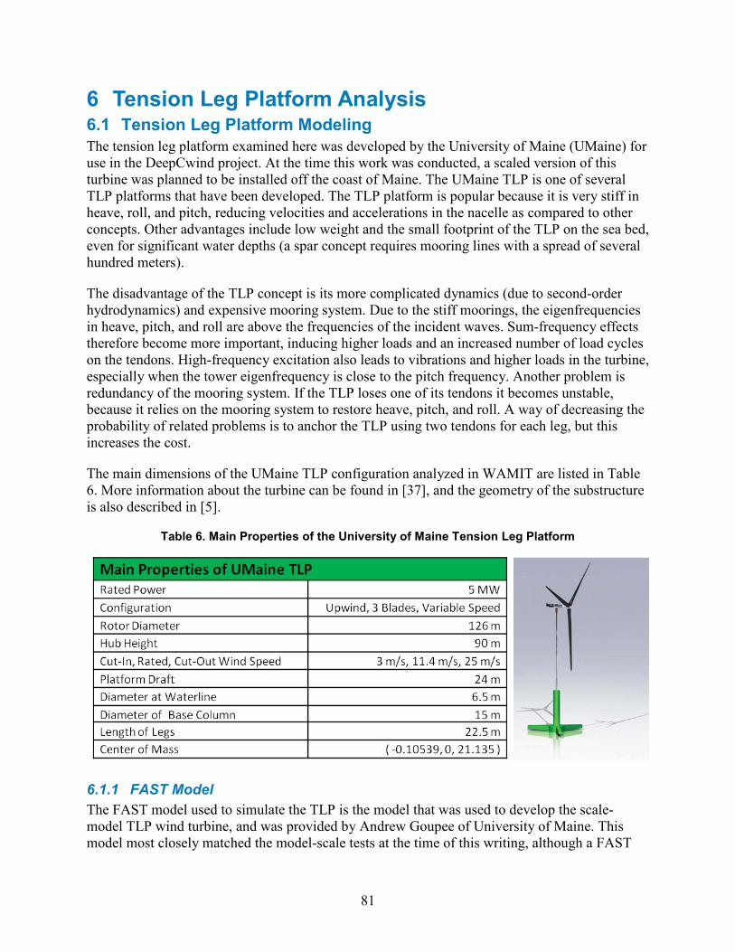
81
6 Tension Leg Platform Analysis 6.1 Tension Leg Platform Modeling The tension leg platform examined here was developed by the University of Maine (UMaine) for use in the DeepCwind project. At the time this work was conducted, a scaled version of this turbine was planned to be installed off the coast of Maine. The UMaine TLP is one of several TLP platforms that have been developed. The TLP platform is popular because it is very stiff in heave, roll, and pitch, reducing velocities and accelerations in the nacelle as compared to other concepts. Other advantages include low weight and the small footprint of the TLP on the sea bed, even for significant water depths (a spar concept requires mooring lines with a spread of several hundred meters).
The disadvantage of the TLP concept is its more complicated dynamics (due to second-order hydrodynamics) and expensive mooring system. Due to the stiff moorings, the eigenfrequencies in heave, pitch, and roll are above the frequencies of the incident waves. Sum-frequency effects therefore become more important, inducing higher loads and an increased number of load cycles on the tendons. High-frequency excitation also leads to vibrations and higher loads in the turbine, especially when the tower eigenfrequency is close to the pitch frequency. Another problem is redundancy of the mooring system. If the TLP loses one of its tendons it becomes unstable, because it relies on the mooring system to restore heave, pitch, and roll. A way of decreasing the probability of related problems is to anchor the TLP using two tendons for each leg, but this increases the cost.
The main dimensions of the UMaine TLP configuration analyzed in WAMIT are listed in Table 6. More information about the turbine can be found in [37], and the geometry of the substructure is also described in [5].
Table 6. Main Properties of the University of Maine Tension Leg Platform
6.1.1 FAST Model The FAST model used to simulate the TLP is the model that was used to develop the scale-model TLP wind turbine, and was provided by Andrew Goupee of University of Maine. This model most closely matched the model-scale tests at the time of this writing, although a FAST
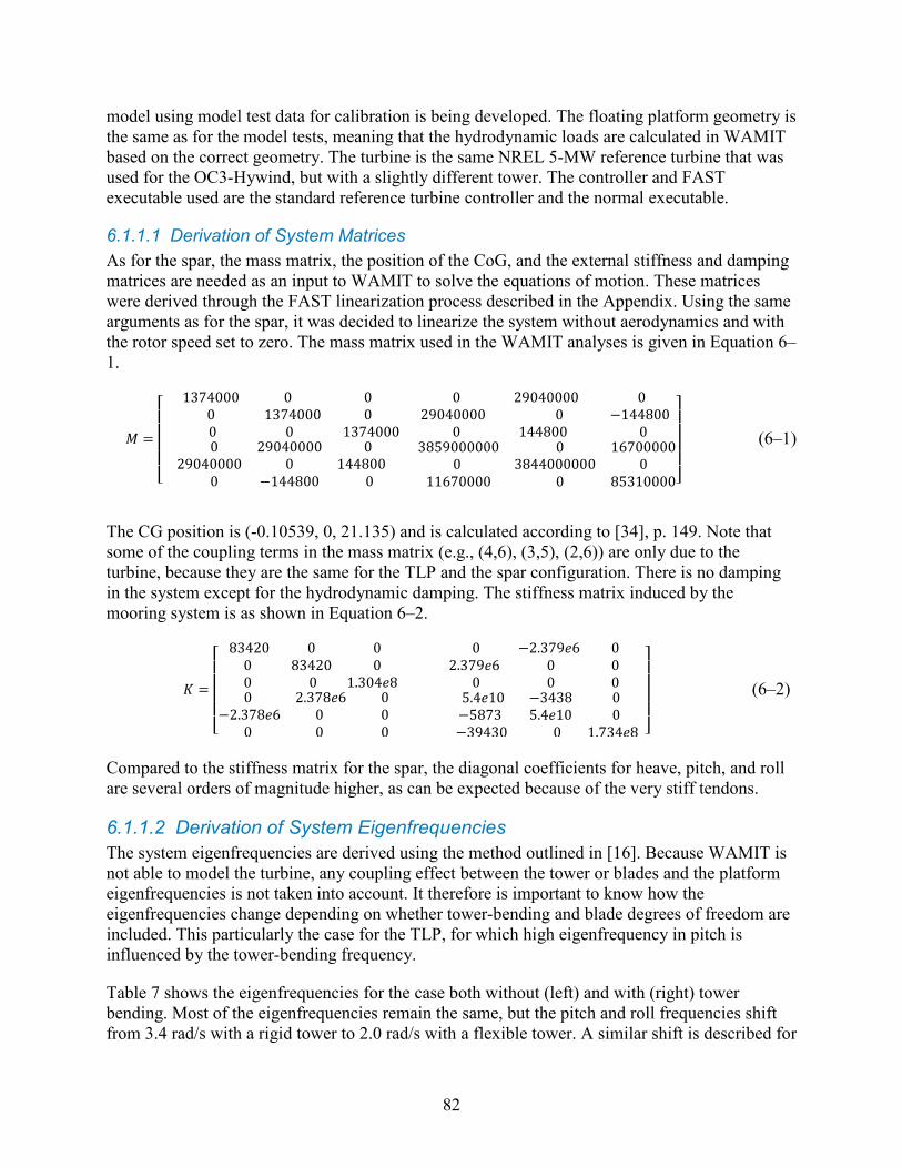
82
model using model test data for calibration is being developed. The floating platform geometry is the same as for the model tests, meaning that the hydrodynamic loads are calculated in WAMIT based on the correct geometry. The turbine is the same NREL 5-MW reference turbine that was used for the OC3-Hywind, but with a slightly different tower. The controller and FAST executable used are the standard reference turbine controller and the normal executable.
6.1.1.1 Derivation of System Matrices As for the spar, the mass matrix, the position of the CoG, and the external stiffness and damping matrices are needed as an input to WAMIT to solve the equations of motion. These matrices were derived through the FAST linearization process described in the Appendix. Using the same arguments as for the spar, it was decided to linearize the system without aerodynamics and with the rotor speed set to zero. The mass matrix used in the WAMIT analyses is given in Equation 6–1.
𝑀 =
⎣⎢⎢⎢⎢⎡ 1374000 0 0
0 1374000 0 0 0 1374000
0 29040000 029040000 0 −144800
0 144800 0 0 29040000 0
29040000 0 144800 0 −144800 0
3859000000 0 167000000 3844000000 0
11670000 0 85310000⎦⎥⎥⎥⎥⎤
(6–1)
The CG position is (-0.10539, 0, 21.135) and is calculated according to [34], p. 149. Note that some of the coupling terms in the mass matrix (e.g., (4,6), (3,5), (2,6)) are only due to the turbine, because they are the same for the TLP and the spar configuration. There is no damping in the system except for the hydrodynamic damping. The stiffness matrix induced by the mooring system is as shown in Equation 6–2.
𝐾 =
⎣⎢⎢⎢⎢⎡
83420 0 00 83420 00 0 1.304𝑒8
0 −2.379𝑒6 0 2.379𝑒6 0 0
0 0 00 2.378𝑒6 0
−2.378𝑒6 0 0 0 0 0
5.4𝑒10 −3438 0−5873 5.4𝑒10 0−39430 0 1.734𝑒8 ⎦
⎥⎥⎥⎥⎤
(6–2)
Compared to the stiffness matrix for the spar, the diagonal coefficients for heave, pitch, and roll are several orders of magnitude higher, as can be expected because of the very stiff tendons.
6.1.1.2 Derivation of System Eigenfrequencies The system eigenfrequencies are derived using the method outlined in [16]. Because WAMIT is not able to model the turbine, any coupling effect between the tower or blades and the platform eigenfrequencies is not taken into account. It therefore is important to know how the eigenfrequencies change depending on whether tower-bending and blade degrees of freedom are included. This particularly the case for the TLP, for which high eigenfrequency in pitch is influenced by the tower-bending frequency.
Table 7 shows the eigenfrequencies for the case both without (left) and with (right) tower bending. Most of the eigenfrequencies remain the same, but the pitch and roll frequencies shift from 3.4 rad/s with a rigid tower to 2.0 rad/s with a flexible tower. A similar shift is described for
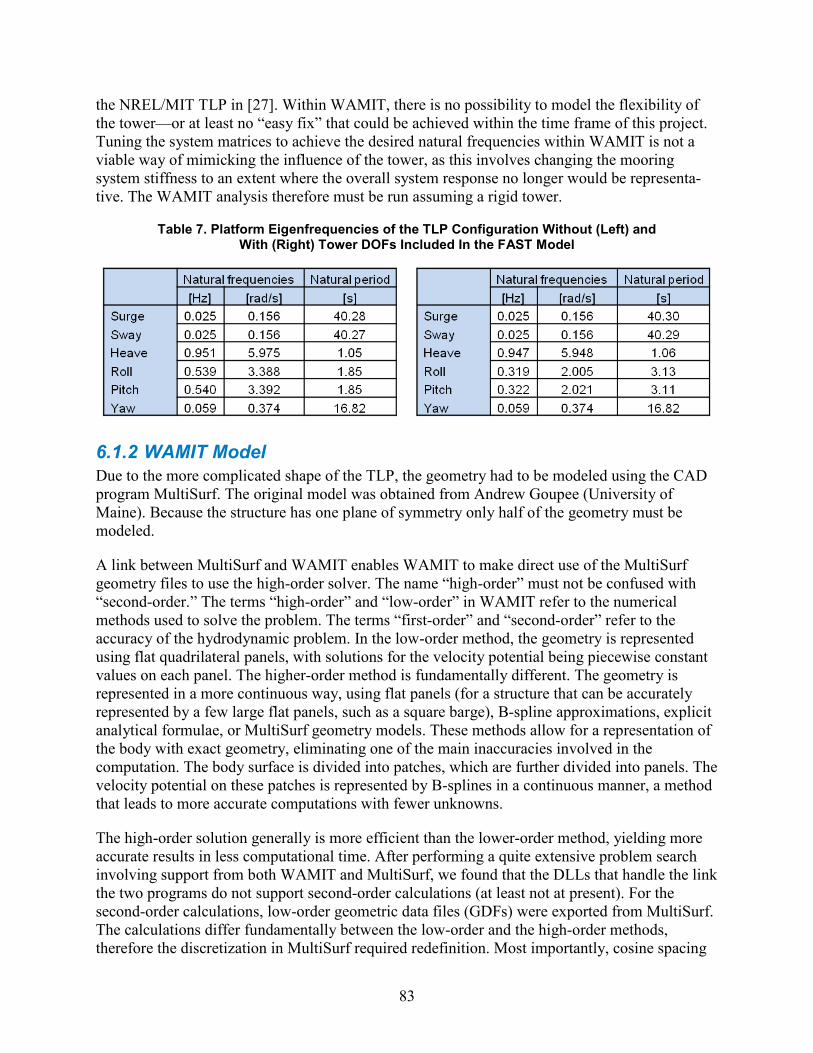
83
the NREL/MIT TLP in [27]. Within WAMIT, there is no possibility to model the flexibility of the tower—or at least no “easy fix” that could be achieved within the time frame of this project. Tuning the system matrices to achieve the desired natural frequencies within WAMIT is not a viable way of mimicking the influence of the tower, as this involves changing the mooring system stiffness to an extent where the overall system response no longer would be representa-tive. The WAMIT analysis therefore must be run assuming a rigid tower.
Table 7. Platform Eigenfrequencies of the TLP Configuration Without (Left) and With (Right) Tower DOFs Included In the FAST Model
6.1.2 WAMIT Model Due to the more complicated shape of the TLP, the geometry had to be modeled using the CAD program MultiSurf. The original model was obtained from Andrew Goupee (University of Maine). Because the structure has one plane of symmetry only half of the geometry must be modeled.
A link between MultiSurf and WAMIT enables WAMIT to make direct use of the MultiSurf geometry files to use the high-order solver. The name “high-order” must not be confused with “second-order.” The terms “high-order” and “low-order” in WAMIT refer to the numerical methods used to solve the problem. The terms “first-order” and “second-order” refer to the accuracy of the hydrodynamic problem. In the low-order method, the geometry is represented using flat quadrilateral panels, with solutions for the velocity potential being piecewise constant values on each panel. The higher-order method is fundamentally different. The geometry is represented in a more continuous way, using flat panels (for a structure that can be accurately represented by a few large flat panels, such as a square barge), B-spline approximations, explicit analytical formulae, or MultiSurf geometry models. These methods allow for a representation of the body with exact geometry, eliminating one of the main inaccuracies involved in the computation. The body surface is divided into patches, which are further divided into panels. The velocity potential on these patches is represented by B-splines in a continuous manner, a method that leads to more accurate computations with fewer unknowns.
The high-order solution generally is more efficient than the lower-order method, yielding more accurate results in less computational time. After performing a quite extensive problem search involving support from both WAMIT and MultiSurf, we found that the DLLs that handle the link the two programs do not support second-order calculations (at least not at present). For the second-order calculations, low-order geometric data files (GDFs) were exported from MultiSurf. The calculations differ fundamentally between the low-order and the high-order methods, therefore the discretization in MultiSurf required redefinition. Most importantly, cosine spacing
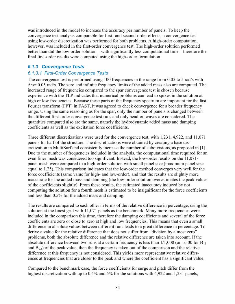
84
was introduced in the model to increase the accuracy per number of panels. To keep the convergence test analysis comparable for first- and second-order effects, a convergence test using low-order discretization was performed for both problems. A high-order computation, however, was included in the first-order convergence test. The high-order solution performed better than did the low-order solution—with significantly less computational time—therefore the final first-order results were computed using the high-order formulation.
6.1.3 Convergence Tests 6.1.3.1 First-Order Convergence Tests The convergence test is performed using 100 frequencies in the range from 0.05 to 5 rad/s with Δω= 0.05 rad/s. The zero and infinite frequency limits of the added mass also are computed. The increased range of frequencies compared to the spar convergence test is chosen because experience with the TLP indicates that numerical problems can lead to spikes in the solution at high or low frequencies. Because these parts of the frequency spectrum are important for the fast Fourier transform (FFT) in FAST, it was agreed to check convergence for a broader frequency range. Using the same reasoning as for the spar, only the number of panels is changed between the different first-order convergence test runs and only head-on waves are considered. The quantities compared also are the same, namely the hydrodynamic added mass and damping coefficients as well as the excitation force coefficients.
Three different discretizations were used for the convergence test, with 1,231, 4,922, and 11,071 panels for half of the structure. The discretizations were obtained by creating a base dis-cretization in MultiSurf and consistently increase the number of subdivisions, as proposed in [1]. Due to the number of frequencies included in the analysis, the computational time required for an even finer mesh was considered too significant. Instead, the low-order results on the 11,071-panel mesh were compared to a high-order solution with small panel size (maximum panel size equal to 1.25). This comparison indicates that the low-order method converges very well for the force coefficients (same value for high- and low-order), and that the results are slightly more inaccurate for the added mass and damping (the low-order solution overestimates the peak values of the coefficients slightly). From these results, the estimated inaccuracy induced by not computing the solution for a fourth mesh is estimated to be insignificant for the force coefficients and less than 0.5% for the added mass and damping.
The results are compared to each other in terms of the relative difference in percentage, using the solution at the finest grid with 11,071 panels as the benchmark. Many more frequencies were included in the comparison this time, therefore the damping coefficients and several of the force coefficients are zero or close to zero at high and low frequencies. This means that even a small difference in absolute values between different runs leads to a great difference in percentage. To derive a value for the relative difference that does not suffer from “division by almost zero” problems, both the absolute difference and the relative difference are taken into account. If the absolute difference between two runs at a certain frequency is less than 1/1,000 (or 1/500 for B11 and B22) of the peak value, then the frequency is taken out of the comparison and the relative difference at this frequency is not considered. This yields more representative relative differ-ences at frequencies that are closer to the peak and where the coefficient has a significant value.
Compared to the benchmark case, the force coefficients for surge and pitch differ from the highest discretization with up to 0.5% and 5% for the solutions with 4,922 and 1,231 panels,
85
respectively. For heave the difference is greater—3.5% and 7.5%—but only as the coefficient drops towards zero at 0.3 rad/s (as shown in Figure 52).
Figure 52. Heave exciting force coefficients for different discretizations
All added mass coefficients converge to within 1.5% for the case with 4,922 panels and 3% for the case with 1,231 panels. The relative differences are about 1.5 times greater for yaw than for other modes, due to the fact that the cylindrical part of the body is represented by flat panels. The damping coefficients converge to within 1% for the case with 4,922 panels and 2% for the case with 1,231 panels. The exceptions are the damping in heave and yaw. The damping of these modes is much greater than for the spar, but still is one order of magnitude (heave) and two orders of magnitude (yaw) smaller than for the other modes. The relative difference for heave and yaw is in the order of 2% with 4,992 panels and 5% with 1,231 panels. Another important effect seen in the convergence tests is that the added mass and damping consistently is over-estimated with a coarser discretization. This is a non-conservative effect that should not be neglected.
6.1.3.2 Second-Order Convergence Tests As explained in Section 5.1, three main parameters influence the second-order solution when using the automatic free-surface mesh option. These parameters are the number of body panels (NPAN), partition radius (PARTR), and the size of the free surface panels (SCALE). The method and the frequencies used for the convergence tests are the same as for the OC3-Hywind.
6.1.3.2.1 NPAN Convergence Tests How the number of body panels influences the second-order results was to be tested with 1,231, 4,922, and 11,071 body panels, with a partition radius of 100 m and the scale parameter set to 2. The 11,071-panel simulation was cancelled due to lack of computer capacity, leaving the only comparison possible being that between 1,231 panels and 4,922 panels. Comparing the two
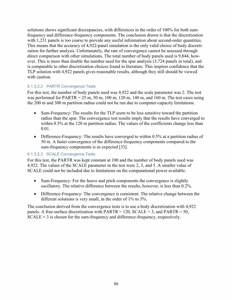
86
solutions shows significant discrepancies, with differences in the order of 100% for both sum-frequency and difference-frequency components. The conclusion drawn is that the discretization with 1,231 panels is too coarse to provide any useful information about second-order quantities. This means that the accuracy of 4,922-panel simulation is the only valid choice of body discreti-zation for further analysis. Unfortunately, the rate of convergence cannot be assessed through direct comparison with other simulations. The total number of body panels used is 9,844, how-ever. This is more than double the number used for the spar analysis (3,724 panels in total), and is comparable to other discretization choices found in literature. This inspires confidence that the TLP solution with 4,922 panels gives reasonable results, although they still should be viewed with caution.
6.1.3.2.2 PARTR Convergence Tests For this test, the number of body panels used was 4,922 and the scale parameter was 2. The test was performed for PARTR = 25 m, 50 m, 100 m, 120 m, 140 m, and 160 m. The test cases using the 200 m and 300 m partition radius could not be run due to computer-capacity limitations.
• Sum-Frequency: The results for the TLP seem to be less sensitive toward the partition radius than the spar. The convergence test results imply that the results have converged to within 0.5% at the 120 m partition radius. The values of the coefficients change less than 0.01.
• Difference-Frequency: The results have converged to within 0.5% at a partition radius of 50 m. A faster convergence of the difference-frequency components compared to the sum-frequency components is as expected [33].
6.1.3.2.3 SCALE Convergence Tests For this test, the PARTR was kept constant at 100 and the number of body panels used was 4,922. The values of the SCALE parameter in the test were 2, 3, and 5. A smaller value of SCALE could not be included due to limitations on the computational power available.
• Sum-Frequency: For the heave and pitch components the convergence is slightly oscillatory. The relative difference between the results, however, is less than 0.2%.
• Difference-Frequency: The convergence is consistent. The relative change between the different solutions is very small, in the order of 1% to 3%.
The conclusion derived from the convergence tests is to use a body discretization with 4,922 panels. A free-surface discretization with PARTR = 120, SCALE = 3, and PARTR = 50, SCALE = 3 is chosen for the sum-frequency and difference-frequency, respectively.
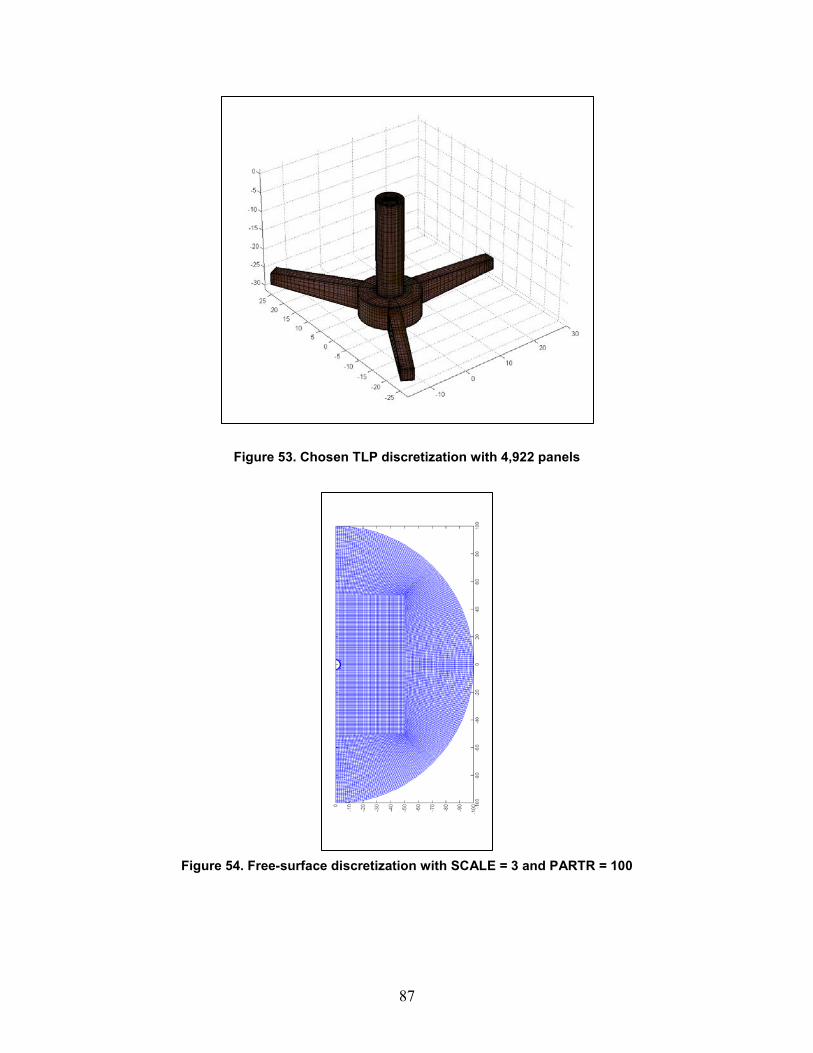
87
Figure 53. Chosen TLP discretization with 4,922 panels
Figure 54. Free-surface discretization with SCALE = 3 and PARTR = 100
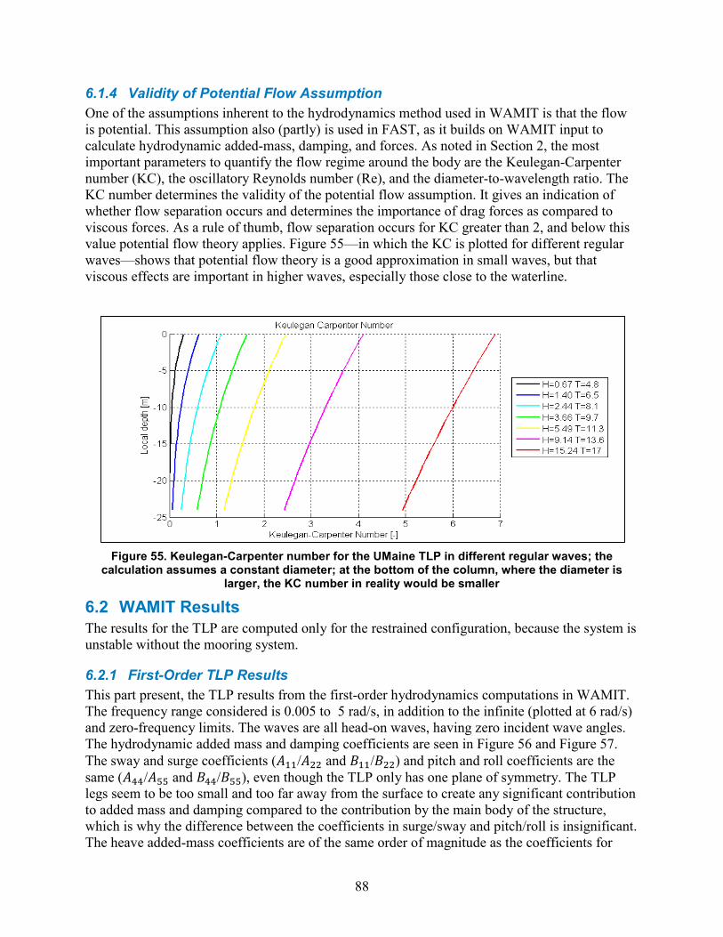
88
6.1.4 Validity of Potential Flow Assumption One of the assumptions inherent to the hydrodynamics method used in WAMIT is that the flow is potential. This assumption also (partly) is used in FAST, as it builds on WAMIT input to calculate hydrodynamic added-mass, damping, and forces. As noted in Section 2, the most important parameters to quantify the flow regime around the body are the Keulegan-Carpenter number (KC), the oscillatory Reynolds number (Re), and the diameter-to-wavelength ratio. The KC number determines the validity of the potential flow assumption. It gives an indication of whether flow separation occurs and determines the importance of drag forces as compared to viscous forces. As a rule of thumb, flow separation occurs for KC greater than 2, and below this value potential flow theory applies. Figure 55—in which the KC is plotted for different regular waves—shows that potential flow theory is a good approximation in small waves, but that viscous effects are important in higher waves, especially those close to the waterline.
Figure 55. Keulegan-Carpenter number for the UMaine TLP in different regular waves; the calculation assumes a constant diameter; at the bottom of the column, where the diameter is
larger, the KC number in reality would be smaller
6.2 WAMIT Results The results for the TLP are computed only for the restrained configuration, because the system is unstable without the mooring system.
6.2.1 First-Order TLP Results This part present, the TLP results from the first-order hydrodynamics computations in WAMIT. The frequency range considered is 0.005 to 5 rad/s, in addition to the infinite (plotted at 6 rad/s) and zero-frequency limits. The waves are all head-on waves, having zero incident wave angles. The hydrodynamic added mass and damping coefficients are seen in Figure 56 and Figure 57. The sway and surge coefficients (𝐴11/𝐴22 and 𝐵11/𝐵22) and pitch and roll coefficients are the same (𝐴44/𝐴55 and 𝐵44/𝐵55), even though the TLP only has one plane of symmetry. The TLP legs seem to be too small and too far away from the surface to create any significant contribution to added mass and damping compared to the contribution by the main body of the structure, which is why the difference between the coefficients in surge/sway and pitch/roll is insignificant. The heave added-mass coefficients are of the same order of magnitude as the coefficients for
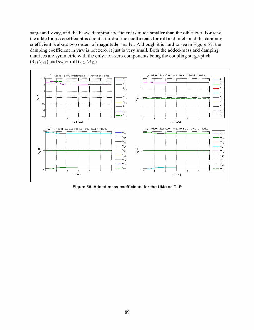
89
surge and sway, and the heave damping coefficient is much smaller than the other two. For yaw, the added-mass coefficient is about a third of the coefficients for roll and pitch, and the damping coefficient is about two orders of magnitude smaller. Although it is hard to see in Figure 57, the damping coefficient in yaw is not zero, it just is very small. Both the added-mass and damping matrices are symmetric with the only non-zero components being the coupling surge-pitch (A15/A51) and sway-roll (A24/A42).
Figure 56. Added-mass coefficients for the UMaine TLP
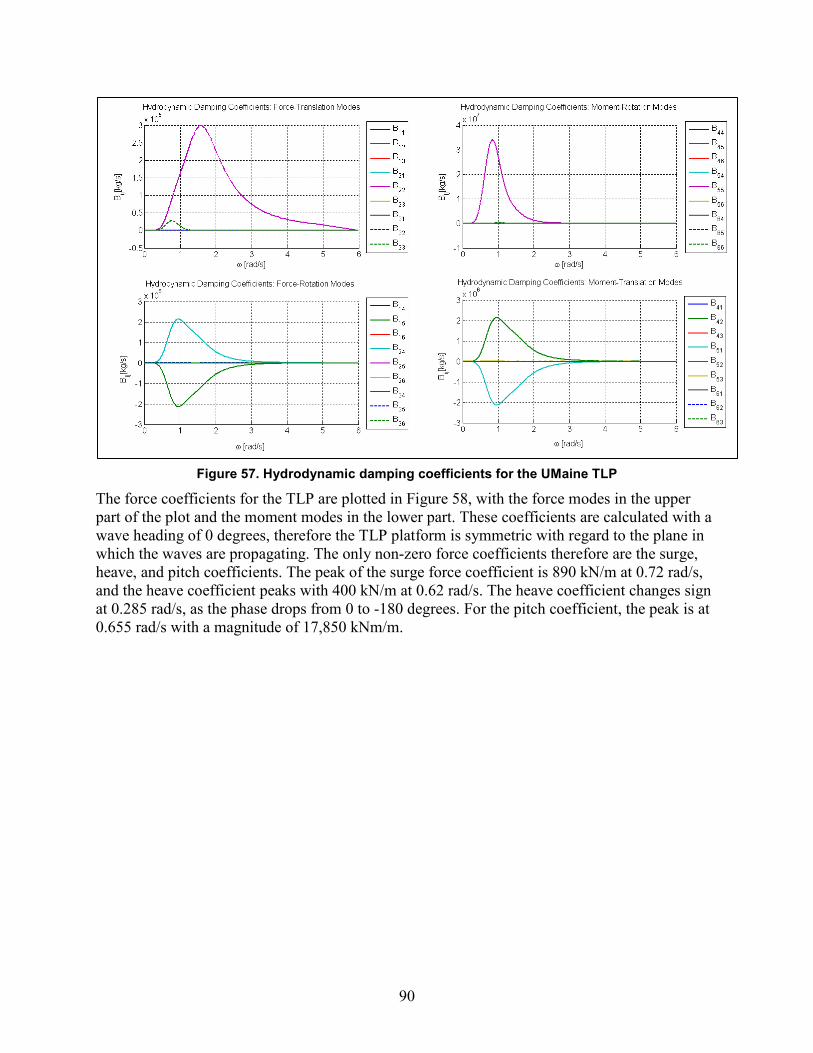
90
Figure 57. Hydrodynamic damping coefficients for the UMaine TLP
The force coefficients for the TLP are plotted in Figure 58, with the force modes in the upper part of the plot and the moment modes in the lower part. These coefficients are calculated with a wave heading of 0 degrees, therefore the TLP platform is symmetric with regard to the plane in which the waves are propagating. The only non-zero force coefficients therefore are the surge, heave, and pitch coefficients. The peak of the surge force coefficient is 890 kN/m at 0.72 rad/s, and the heave coefficient peaks with 400 kN/m at 0.62 rad/s. The heave coefficient changes sign at 0.285 rad/s, as the phase drops from 0 to -180 degrees. For the pitch coefficient, the peak is at 0.655 rad/s with a magnitude of 17,850 kNm/m.
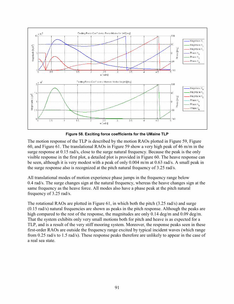
91
Figure 58. Exciting force coefficients for the UMaine TLP
The motion response of the TLP is described by the motion RAOs plotted in Figure 59, Figure 60, and Figure 61. The translational RAOs in Figure 59 show a very high peak of 46 m/m in the surge response at 0.15 rad/s, close to the surge natural frequency. Because the peak is the only visible response in the first plot, a detailed plot is provided in Figure 60. The heave response can be seen, although it is very modest with a peak of only 0.004 m/m at 0.63 rad/s. A small peak in the surge response also is recognized at the pitch natural frequency of 3.25 rad/s.
All translational modes of motion experience phase jumps in the frequency range below 0.4 rad/s. The surge changes sign at the natural frequency, whereas the heave changes sign at the same frequency as the heave force. All modes also have a phase peak at the pitch natural frequency of 3.25 rad/s.
The rotational RAOs are plotted in Figure 61, in which both the pitch (3.25 rad/s) and surge (0.15 rad/s) natural frequencies are shown as peaks in the pitch response. Although the peaks are high compared to the rest of the response, the magnitudes are only 0.14 deg/m and 0.09 deg/m. That the system exhibits only very small motions both for pitch and heave is as expected for a TLP, and is a result of the very stiff mooring system. Moreover, the response peaks seen in these first-order RAOs are outside the frequency range excited by typical incident waves (which range from 0.25 rad/s to 1.5 rad/s). These response peaks therefore are unlikely to appear in the case of a real sea state.
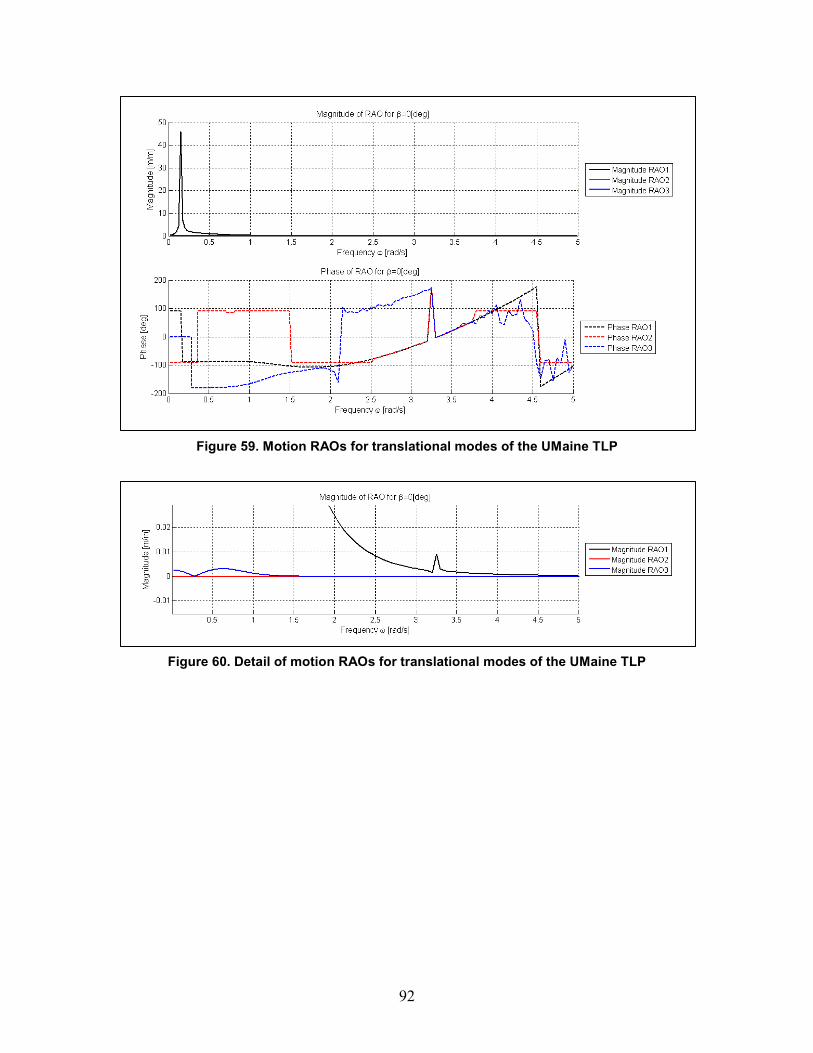
92
Figure 59. Motion RAOs for translational modes of the UMaine TLP
Figure 60. Detail of motion RAOs for translational modes of the UMaine TLP
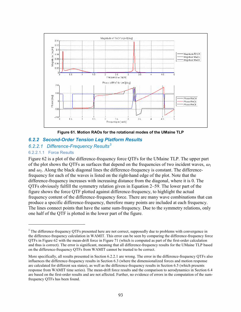
93
Figure 61. Motion RAOs for the rotational modes of the UMaine TLP
6.2.2 Second-Order Tension Leg Platform Results 6.2.2.1 Difference-Frequency Results3 6.2.2.1.1 Force Results Figure 62 is a plot of the difference-frequency force QTFs for the UMaine TLP. The upper part of the plot shows the QTFs as surfaces that depend on the frequencies of two incident waves, ω1 and ω2. Along the black diagonal lines the difference-frequency is constant. The difference-frequency for each of the waves is listed on the right-hand edge of the plot. Note that the difference-frequency increases with increasing distance from the diagonal, where it is 0. The QTFs obviously fulfill the symmetry relation given in Equation 2–59. The lower part of the figure shows the force QTF plotted against difference-frequency, to highlight the actual frequency content of the difference-frequency force. There are many wave combinations that can produce a specific difference-frequency, therefore many points are included at each frequency. The lines connect points that have the same sum-frequency. Due to the symmetry relations, only one half of the QTF is plotted in the lower part of the figure.
3 The difference-frequency QTFs presented here are not correct, supposedly due to problems with convergence in the difference-frequency calculation in WAMIT. This error can be seen by comparing the difference-frequency force QTFs in Figure 62 with the mean-drift force in Figure 71 (which is computed as part of the first-order calculation and thus is correct). The error is significant, meaning that all difference-frequency results for the UMaine TLP based on the difference-frequency QTFs from WAMIT cannot be trusted to be correct.
More specifically, all results presented in Section 6.2.2.1 are wrong. The error in the difference-frequency QTFs also influences the difference-frequency results in Section 6.3 (where the dimensionalized forces and motion response are calculated for different sea states), as well as the difference-frequency results in Section 6.5 (which presents response from WAMIT time series). The mean-drift force results and the comparison to aerodynamics in Section 6.4 are based on the first-order results and are not affected. Further, no evidence of errors in the computation of the sum-frequency QTFs has been found.
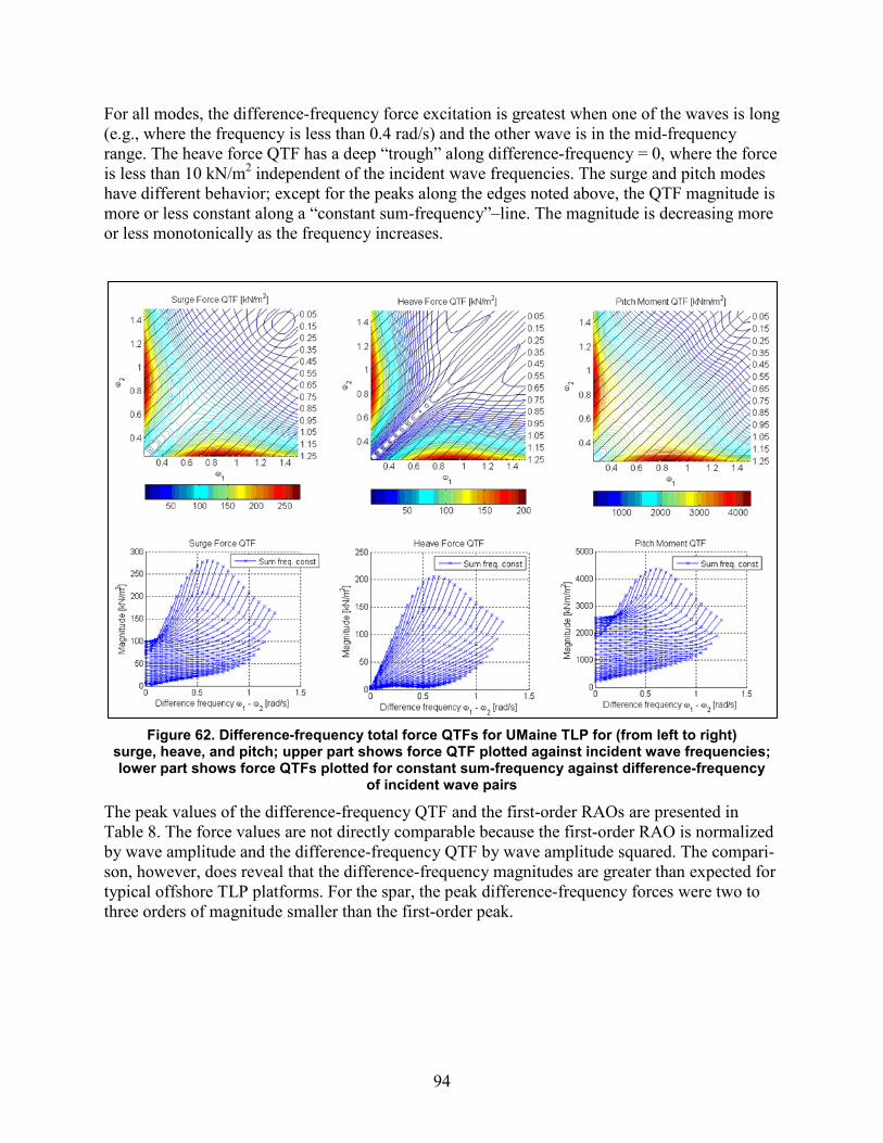
94
For all modes, the difference-frequency force excitation is greatest when one of the waves is long (e.g., where the frequency is less than 0.4 rad/s) and the other wave is in the mid-frequency range. The heave force QTF has a deep “trough” along difference-frequency = 0, where the force is less than 10 kN/m2 independent of the incident wave frequencies. The surge and pitch modes have different behavior; except for the peaks along the edges noted above, the QTF magnitude is more or less constant along a “constant sum-frequency”–line. The magnitude is decreasing more or less monotonically as the frequency increases.
Figure 62. Difference-frequency total force QTFs for UMaine TLP for (from left to right) surge, heave, and pitch; upper part shows force QTF plotted against incident wave frequencies; lower part shows force QTFs plotted for constant sum-frequency against difference-frequency
of incident wave pairs
The peak values of the difference-frequency QTF and the first-order RAOs are presented in Table 8. The force values are not directly comparable because the first-order RAO is normalized by wave amplitude and the difference-frequency QTF by wave amplitude squared. The compari-son, however, does reveal that the difference-frequency magnitudes are greater than expected for typical offshore TLP platforms. For the spar, the peak difference-frequency forces were two to three orders of magnitude smaller than the first-order peak.
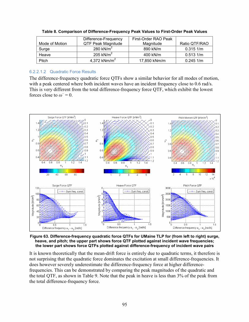
95
Table 8. Comparison of Difference-Frequency Peak Values to First-Order Peak Values
Mode of Motion Difference-Frequency QTF Peak Magnitude
First-Order RAO Peak Magnitude Ratio QTF/RAO
Surge 280 kN/m2 890 kN/m 0.315 1/m Heave 205 kN/m2 400 kN/m 0.513 1/m Pitch 4,372 kNm/m2 17,850 kNm/m 0.245 1/m
6.2.2.1.2 Quadratic Force Results The difference-frequency quadratic force QTFs show a similar behavior for all modes of motion, with a peak centered where both incident waves have an incident frequency close to 0.6 rad/s. This is very different from the total difference-frequency force QTF, which exhibit the lowest forces close to ω– = 0.
Figure 63. Difference-frequency quadratic force QTFs for UMaine TLP for (from left to right) surge, heave, and pitch; the upper part shows force QTF plotted against incident wave frequencies; the lower part shows force QTFs plotted against difference-frequency of incident wave pairs
It is known theoretically that the mean-drift force is entirely due to quadratic terms, it therefore is not surprising that the quadratic force dominates the excitation at small difference-frequencies. It does however severely underestimate the difference-frequency force at higher difference-frequencies. This can be demonstrated by comparing the peak magnitudes of the quadratic and the total QTF, as shown in Table 9. Note that the peak in heave is less than 3% of the peak from the total difference-frequency force.
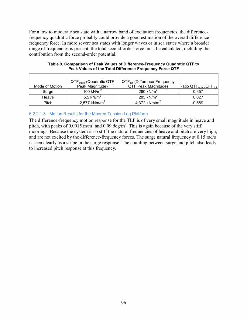
96
For a low to moderate sea state with a narrow band of excitation frequencies, the difference-frequency quadratic force probably could provide a good estimation of the overall difference-frequency force. In more severe sea states with longer waves or in sea states where a broader range of frequencies is present, the total second-order force must be calculated, including the contribution from the second-order potential.
Table 9. Comparison of Peak Values of Difference-Frequency Quadratic QTF to Peak Values of the Total Difference-Frequency Force QTF
Mode of Motion QTFquad (Quadratic QTF
Peak Magnitude) QTFtot (Difference-Frequency
QTF Peak Magnitude) Ratio QTFquad/QTFtot Surge 100 kN/m2 280 kN/m2 0.357 Heave 5.5 kN/m2 205 kN/m2 0.027 Pitch 2,577 kNm/m2 4,372 kNm/m2 0.589
6.2.2.1.3 Motion Results for the Moored Tension Leg Platform The difference-frequency motion response for the TLP is of very small magnitude in heave and pitch, with peaks of 0.0015 m/m2 and 0.09 deg/m2. This is again because of the very stiff moorings. Because the system is so stiff the natural frequencies of heave and pitch are very high, and are not excited by the difference-frequency forces. The surge natural frequency at 0.15 rad/s is seen clearly as a stripe in the surge response. The coupling between surge and pitch also leads to increased pitch response at this frequency.
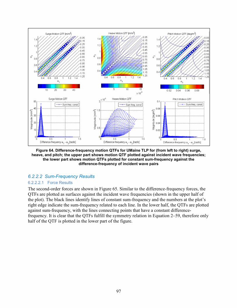
97
Figure 64. Difference-frequency motion QTFs for UMaine TLP for (from left to right) surge, heave, and pitch; the upper part shows motion QTF plotted against incident wave frequencies;
the lower part shows motion QTFs plotted for constant sum-frequency against the difference-frequency of incident wave pairs
6.2.2.2 Sum-Frequency Results 6.2.2.2.1 Force Results The second-order forces are shown in Figure 65. Similar to the difference-frequency forces, the QTFs are plotted as surfaces against the incident wave frequencies (shown in the upper half of the plot). The black lines identify lines of constant sum-frequency and the numbers at the plot’s right edge indicate the sum-frequency related to each line. In the lower half, the QTFs are plotted against sum-frequency, with the lines connecting points that have a constant difference-frequency. It is clear that the QTFs fulfill the symmetry relation in Equation 2–59, therefore only half of the QTF is plotted in the lower part of the figure.
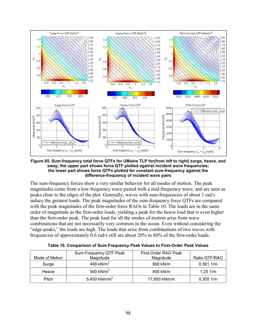
98
Figure 65. Sum-frequency total force QTFs for UMaine TLP for(from left to right) surge, heave, and sway; the upper part shows force QTF plotted against incident wave frequencies; the lower part shows force QTFs plotted for constant sum-frequency against the
difference-frequency of incident wave pairs
The sum-frequency forces show a very similar behavior for all modes of motion. The peak magnitudes come from a low-frequency wave paired with a mid-frequency wave, and are seen as peaks close to the edges of the plot. Generally, waves with sum-frequencies of about 1 rad/s induce the greatest loads. The peak magnitudes of the sum-frequency force QTFs are compared with the peak magnitudes of the first-order force RAOs in Table 10. The loads are in the same order of magnitude as the first-order loads, yielding a peak for the heave load that is even higher than the first-order peak. The peak load for all the modes of motion arise from wave combinations that are not necessarily very common in the ocean. Even without considering the “edge-peaks,” the loads are high. The loads that arise from combinations of two waves with frequencies of approximately 0.6 rad/s still are about 20% to 80% of the first-order loads.
Table 10. Comparison of Sum-Frequency Peak Values to First-Order Peak Values
Mode of Motion Sum-Frequency QTF Peak
Magnitude First-Order RAO Peak
Magnitude Ratio QTF/RAO Surge 499 kN/m2 890 kN/m 0.561 1/m
Heave 500 kN/m2 400 kN/m 1.25 1/m
Pitch 5,450 kNm/m2 17,850 kNm/m 0.305 1/m
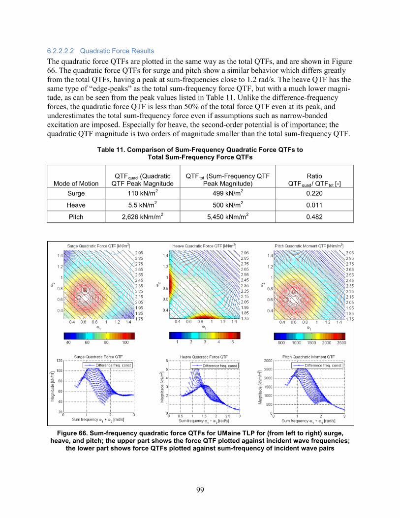
99
6.2.2.2.2 Quadratic Force Results The quadratic force QTFs are plotted in the same way as the total QTFs, and are shown in Figure 66. The quadratic force QTFs for surge and pitch show a similar behavior which differs greatly from the total QTFs, having a peak at sum-frequencies close to 1.2 rad/s. The heave QTF has the same type of “edge-peaks” as the total sum-frequency force QTF, but with a much lower magni-tude, as can be seen from the peak values listed in Table 11. Unlike the difference-frequency forces, the quadratic force QTF is less than 50% of the total force QTF even at its peak, and underestimates the total sum-frequency force even if assumptions such as narrow-banded excitation are imposed. Especially for heave, the second-order potential is of importance; the quadratic QTF magnitude is two orders of magnitude smaller than the total sum-frequency QTF.
Table 11. Comparison of Sum-Frequency Quadratic Force QTFs to Total Sum-Frequency Force QTFs
Mode of Motion QTFquad (Quadratic
QTF Peak Magnitude QTFtot (Sum-Frequency QTF
Peak Magnitude) Ratio
QTFquad/ QTFtot [-] Surge 110 kN/m2 499 kN/m2 0.220
Heave 5.5 kN/m2 500 kN/m2 0.011
Pitch 2,626 kNm/m2 5,450 kNm/m2 0.482
Figure 66. Sum-frequency quadratic force QTFs for UMaine TLP for (from left to right) surge, heave, and pitch; the upper part shows the force QTF plotted against incident wave frequencies;
the lower part shows force QTFs plotted against sum-frequency of incident wave pairs
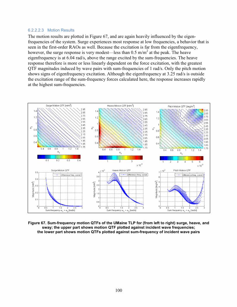
100
6.2.2.2.3 Motion Results The motion results are plotted in Figure 67, and are again heavily influenced by the eigen-frequencies of the system. Surge experiences most response at low frequencies, a behavior that is seen in the first-order RAOs as well. Because the excitation is far from the eigenfrequency, however, the surge response is very modest—less than 0.5 m/m2 at the peak. The heave eigenfrequency is at 6.04 rad/s, above the range excited by the sum-frequencies. The heave response therefore is more or less linearly dependent on the force excitation, with the greatest QTF magnitudes induced by wave pairs with sum-frequencies of 1 rad/s. Only the pitch motion shows signs of eigenfrequency excitation. Although the eigenfrequency at 3.25 rad/s is outside the excitation range of the sum-frequency forces calculated here, the response increases rapidly at the highest sum-frequencies.
Figure 67. Sum-frequency motion QTFs of the UMaine TLP for (from left to right) surge, heave, and
sway; the upper part shows motion QTF plotted against incident wave frequencies; the lower part shows motion QTFs plotted against sum-frequency of incident wave pairs
101
6.3 Comparison of First-Order and Second-Order Forces and Motions in Different Environments4
The first-order RAOs and second-order QTFs cannot be compared to each other directly, because the first-order quantities are normalized with the incident wave amplitude and the second-order quantities are normalized by incident wave amplitude squared. To enable comparison, the forces and motions first must be dimensionalized by the wave amplitudes of a given sea state. The choice of an incident wave spectrum and random phases influences the result, and the comparison therefore should be repeated for a range of different environmental conditions. The goal of the comparison is to assess the total excitation and response at a given frequency, but there are many different incident wave pairs that contribute to the same sum- or difference-frequency. Therefore, all second-order contributions at a certain sum-frequency or difference-frequency are summed together to get the total response at this frequency (described in Section 5.4). The second-order contributions are computed for fifteen different realizations of the sea state to give an impression of the magnitude range of the total response (which differs between realizations because it depends on the random phases of the incident waves).
In the plots shown below, the first-order RAO is rendered as a black line. The magnitude of the first-order quantities is the same in all realizations of the sea state because the wave amplitudes are determined directly from the spectrum, without any randomness included. The magnitude does change between sea states, however, because the wave amplitude for a given frequency is changing. In the figures, the difference-frequency contribution from each realization is plotted as green crosses for every frequency, with the mean computed from the fifteen realizations shown as a red line. The sum-frequency contribution is shown in a similar way, with light blue dots denoting the contribution from one realization and a dark blue line showing the mean among the realizations.
The comparison was made for all twelve environmental conditions in Table 1, but the results are shown only for sea states 4, 7, and 11. These results were found to be representative for different groups of environmental conditions.
• Sea state 4 (Hs = 1.44 m, Tp = 6.5 s): Low sea states with operating turbine
• Sea state 7 (Hs = 3.66 m, Tp = 9.7 s): Moderate sea states with operating turbine
• Sea state 11 (Hs = 9.14 m, Tp = 13.6 s): Severe sea state with idling turbine
In the lower sea states (Figure 68), the second-order forces are modest, with the sum-frequency force in heave being the highest. The surge response is dominated by the difference-frequency response, and a coupling to this difference-frequency response also appears in pitch. The second-order forces were calculated only for the frequency range between 0.25 and 1.5 rad/s, which means that the highest sum-frequency excitation is at 3 rad/s. This is below both the pitch (3.25 rad/s) and heave (6 rad/s) natural frequency, therefore no sum-frequency response occurs at this frequency. The Pierson-Moscowitz spectrum has a long tail to high frequencies, however, therefore the pitch natural frequency actually is excited by the first-order waves in the sea states
4 The difference-frequency results presented in this section are affected by the error in the QTF calculation as described in Section 6.2.2.1.
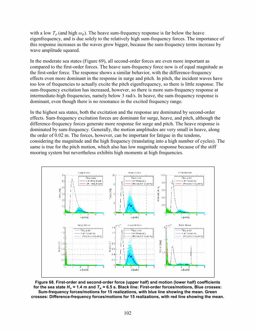
102
with a low Tp (and high ωp). The heave sum-frequency response is far below the heave eigenfrequency, and is due solely to the relatively high sum-frequency forces. The importance of this response increases as the waves grow bigger, because the sum-frequency terms increase by wave amplitude squared.
In the moderate sea states (Figure 69), all second-order forces are even more important as compared to the first-order forces. The heave sum-frequency force now is of equal magnitude as the first-order force. The response shows a similar behavior, with the difference-frequency effects even more dominant in the response in surge and pitch. In pitch, the incident waves have too low of frequencies to actually excite the pitch eigenfrequency, so there is little response. The sum-frequency excitation has increased, however, so there is more sum-frequency response at intermediate-high frequencies, namely below 3 rad/s. In heave, the sum-frequency response is dominant, even though there is no resonance in the excited frequency range.
In the highest sea states, both the excitation and the response are dominated by second-order effects. Sum-frequency excitation forces are dominant for surge, heave, and pitch, although the difference-frequency forces generate more response for surge and pitch. The heave response is dominated by sum-frequency. Generally, the motion amplitudes are very small in heave, along the order of 0.02 m. The forces, however, can be important for fatigue in the tendons, considering the magnitude and the high frequency (translating into a high number of cycles). The same is true for the pitch motion, which also has low magnitude response because of the stiff mooring system but nevertheless exhibits high moments at high frequencies.
Figure 68. First-order and second-order force (upper half) and motion (lower half) coefficients for the sea state Hs = 1.4 m and Tp = 6.5 s. Black line: First-order forces/motions, Blue crosses:
Sum-frequency forces/motions for 15 realizations, with blue line showing the mean. Green crosses: Difference-frequency forces/motions for 15 realizations, with red line showing the mean.
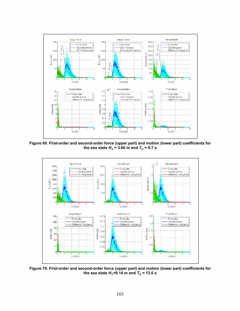
103
Figure 69. First-order and second-order force (upper part) and motion (lower part) coefficients for the sea state Hs = 3.66 m and Tp = 9.7 s
Figure 70. First-order and second-order force (upper part) and motion (lower part) coefficients for the sea state Hs=9.14 m and Tp = 13.6 s
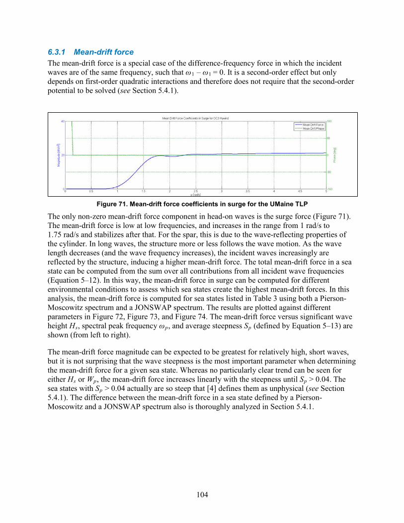
104
6.3.1 Mean-drift force The mean-drift force is a special case of the difference-frequency force in which the incident waves are of the same frequency, such that ω1 – ω1 = 0. It is a second-order effect but only depends on first-order quadratic interactions and therefore does not require that the second-order potential to be solved (see Section 5.4.1).
Figure 71. Mean-drift force coefficients in surge for the UMaine TLP
The only non-zero mean-drift force component in head-on waves is the surge force (Figure 71). The mean-drift force is low at low frequencies, and increases in the range from 1 rad/s to 1.75 rad/s and stabilizes after that. For the spar, this is due to the wave-reflecting properties of the cylinder. In long waves, the structure more or less follows the wave motion. As the wave length decreases (and the wave frequency increases), the incident waves increasingly are reflected by the structure, inducing a higher mean-drift force. The total mean-drift force in a sea state can be computed from the sum over all contributions from all incident wave frequencies (Equation 5–12). In this way, the mean-drift force in surge can be computed for different environmental conditions to assess which sea states create the highest mean-drift forces. In this analysis, the mean-drift force is computed for sea states listed in Table 3 using both a Pierson-Moscowitz spectrum and a JONSWAP spectrum. The results are plotted against different parameters in Figure 72, Figure 73, and Figure 74. The mean-drift force versus significant wave height Hs, spectral peak frequency ωp, and average steepness Sp (defined by Equation 5–13) are shown (from left to right).
The mean-drift force magnitude can be expected to be greatest for relatively high, short waves, but it is not surprising that the wave steepness is the most important parameter when determining the mean-drift force for a given sea state. Whereas no particularly clear trend can be seen for either Hs or Wp, the mean-drift force increases linearly with the steepness until Sp > 0.04. The sea states with Sp > 0.04 actually are so steep that [4] defines them as unphysical (see Section 5.4.1). The difference between the mean-drift force in a sea state defined by a Pierson-Moscowitz and a JONSWAP spectrum also is thoroughly analyzed in Section 5.4.1.
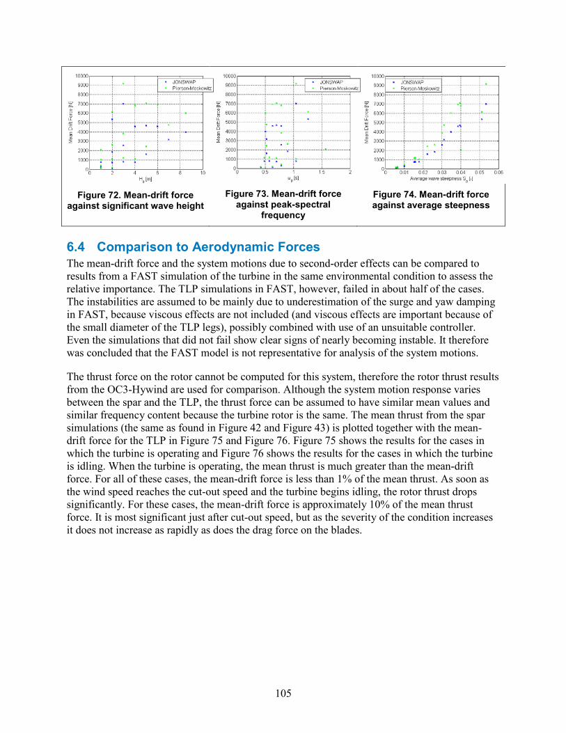
105
Figure 72. Mean-drift force
against significant wave height
Figure 73. Mean-drift force
against peak-spectral frequency
Figure 74. Mean-drift force against average steepness
6.4 Comparison to Aerodynamic Forces The mean-drift force and the system motions due to second-order effects can be compared to results from a FAST simulation of the turbine in the same environmental condition to assess the relative importance. The TLP simulations in FAST, however, failed in about half of the cases. The instabilities are assumed to be mainly due to underestimation of the surge and yaw damping in FAST, because viscous effects are not included (and viscous effects are important because of the small diameter of the TLP legs), possibly combined with use of an unsuitable controller. Even the simulations that did not fail show clear signs of nearly becoming instable. It therefore was concluded that the FAST model is not representative for analysis of the system motions.
The thrust force on the rotor cannot be computed for this system, therefore the rotor thrust results from the OC3-Hywind are used for comparison. Although the system motion response varies between the spar and the TLP, the thrust force can be assumed to have similar mean values and similar frequency content because the turbine rotor is the same. The mean thrust from the spar simulations (the same as found in Figure 42 and Figure 43) is plotted together with the mean-drift force for the TLP in Figure 75 and Figure 76. Figure 75 shows the results for the cases in which the turbine is operating and Figure 76 shows the results for the cases in which the turbine is idling. When the turbine is operating, the mean thrust is much greater than the mean-drift force. For all of these cases, the mean-drift force is less than 1% of the mean thrust. As soon as the wind speed reaches the cut-out speed and the turbine begins idling, the rotor thrust drops significantly. For these cases, the mean-drift force is approximately 10% of the mean thrust force. It is most significant just after cut-out speed, but as the severity of the condition increases it does not increase as rapidly as does the drag force on the blades.
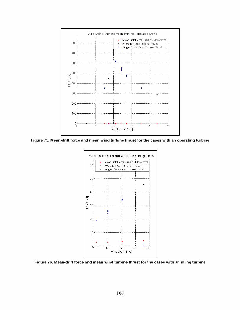
106
Figure 75. Mean-drift force and mean wind turbine thrust for the cases with an operating turbine
Figure 76. Mean-drift force and mean wind turbine thrust for the cases with an idling turbine
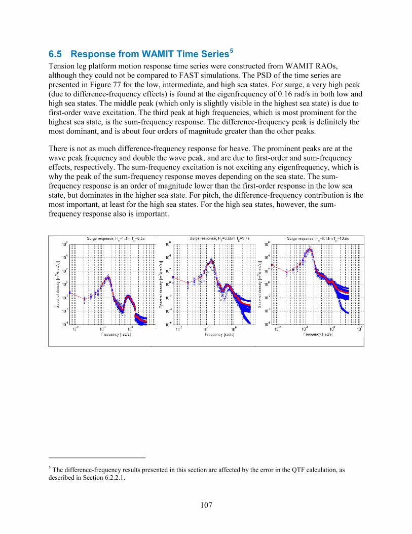
107
6.5 Response from WAMIT Time Series5 Tension leg platform motion response time series were constructed from WAMIT RAOs, although they could not be compared to FAST simulations. The PSD of the time series are presented in Figure 77 for the low, intermediate, and high sea states. For surge, a very high peak (due to difference-frequency effects) is found at the eigenfrequency of 0.16 rad/s in both low and high sea states. The middle peak (which only is slightly visible in the highest sea state) is due to first-order wave excitation. The third peak at high frequencies, which is most prominent for the highest sea state, is the sum-frequency response. The difference-frequency peak is definitely the most dominant, and is about four orders of magnitude greater than the other peaks.
There is not as much difference-frequency response for heave. The prominent peaks are at the wave peak frequency and double the wave peak, and are due to first-order and sum-frequency effects, respectively. The sum-frequency excitation is not exciting any eigenfrequency, which is why the peak of the sum-frequency response moves depending on the sea state. The sum-frequency response is an order of magnitude lower than the first-order response in the low sea state, but dominates in the higher sea state. For pitch, the difference-frequency contribution is the most important, at least for the high sea states. For the high sea states, however, the sum-frequency response also is important.
5 The difference-frequency results presented in this section are affected by the error in the QTF calculation, as described in Section 6.2.2.1.
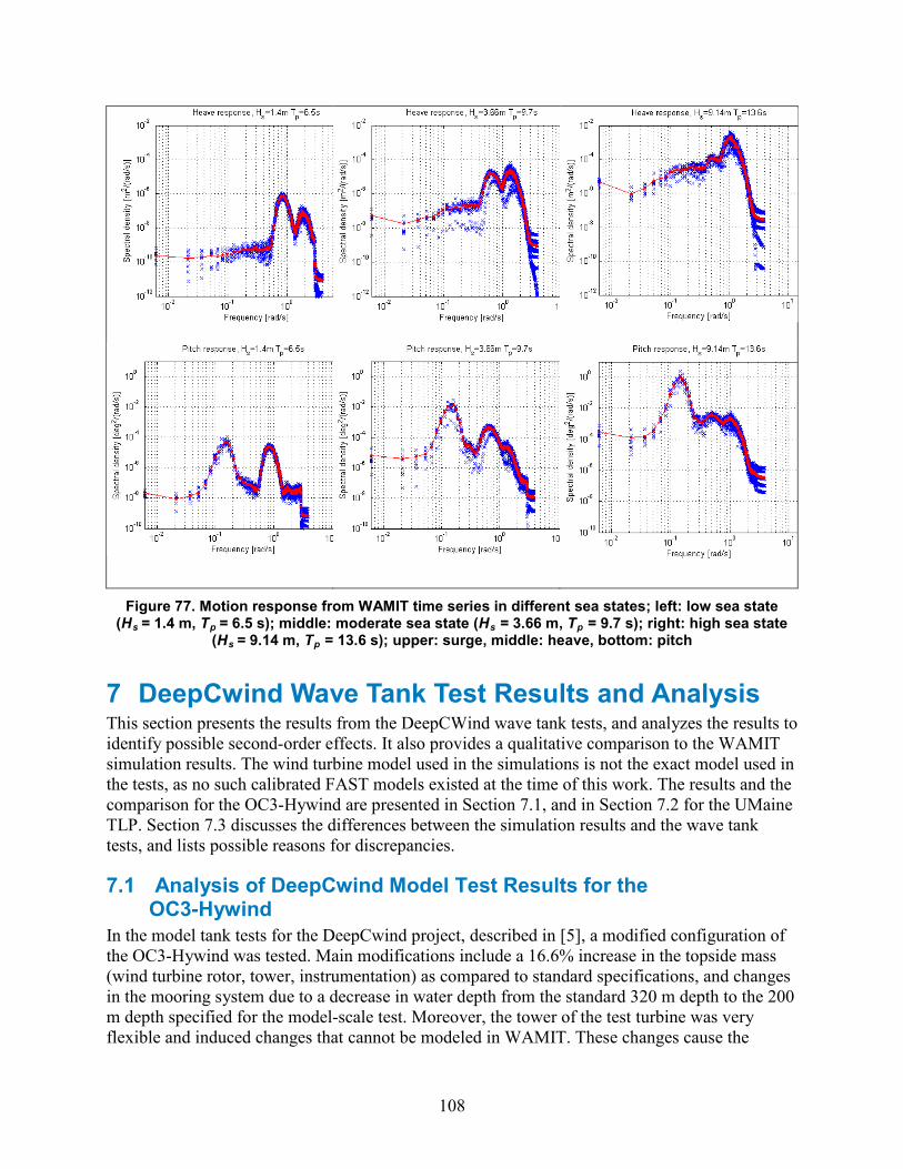
108
Figure 77. Motion response from WAMIT time series in different sea states; left: low sea state (Hs = 1.4 m, Tp = 6.5 s); middle: moderate sea state (Hs = 3.66 m, Tp = 9.7 s); right: high sea state
(Hs = 9.14 m, Tp = 13.6 s); upper: surge, middle: heave, bottom: pitch
7 DeepCwind Wave Tank Test Results and Analysis This section presents the results from the DeepCWind wave tank tests, and analyzes the results to identify possible second-order effects. It also provides a qualitative comparison to the WAMIT simulation results. The wind turbine model used in the simulations is not the exact model used in the tests, as no such calibrated FAST models existed at the time of this work. The results and the comparison for the OC3-Hywind are presented in Section 7.1, and in Section 7.2 for the UMaine TLP. Section 7.3 discusses the differences between the simulation results and the wave tank tests, and lists possible reasons for discrepancies.
7.1 Analysis of DeepCwind Model Test Results for the OC3-Hywind
In the model tank tests for the DeepCwind project, described in [5], a modified configuration of the OC3-Hywind was tested. Main modifications include a 16.6% increase in the topside mass (wind turbine rotor, tower, instrumentation) as compared to standard specifications, and changes in the mooring system due to a decrease in water depth from the standard 320 m depth to the 200 m depth specified for the model-scale test. Moreover, the tower of the test turbine was very flexible and induced changes that cannot be modeled in WAMIT. These changes cause the
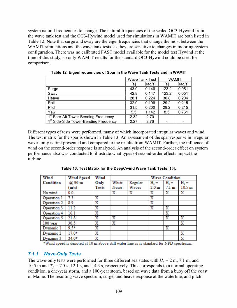
109
system natural frequencies to change. The natural frequencies of the scaled OC3-Hywind from the wave tank test and the OC3-Hywind model used for simulations in WAMIT are both listed in Table 12. Note that surge and sway are the eigenfrequencies that change the most between the WAMIT simulations and the wave tank tests, as they are sensitive to changes in mooring-system configuration. There was no calibrated FAST model available for the model test Hywind at the time of this study, so only WAMIT results for the standard OC3-Hywind could be used for comparison.
Table 12. Eigenfrequencies of Spar in the Wave Tank Tests and in WAMIT
Wave Tank Test WAMIT
[s] [rad/s] [s] [rad/s] Surge 43.0 0.146 123.2 0.051 Sway 42.8 0.147 123.2 0.051 Heave 28.1 0.224 30.8 0.204 Roll 32.0 0.196 29.2 0.215 Pitch 31.5 0.200 29.2 0.215 Yaw 5.5 1.142 8.3 0.761 1st Fore-Aft Tower-Bending Frequency 2.32 2.70 - - 1st Side-Side Tower-Bending Frequency 2.27 2.76 - -
Different types of tests were performed, many of which incorporated irregular waves and wind. The test matrix for the spar is shown in Table 13. An assessment of the spar response in irregular waves only is first presented and compared to the results from WAMIT. Further, the influence of wind on the second-order response is analyzed. An analysis of the second-order effect on system performance also was conducted to illustrate what types of second-order effects impact the turbine.
Table 13. Test Matrix for the DeepCwind Wave Tank Tests [10].
7.1.1 Wave-Only Tests The wave-only tests were performed for three different sea states with Hs = 2 m, 7.1 m, and 10.5 m and Tp = 7.5 s, 12.1 s, and 14.3 s, respectively. This corresponds to a normal operating condition, a one-year storm, and a 100-year storm, based on wave data from a buoy off the coast of Maine. The resulting wave spectrum, surge, and heave response at the waterline, and pitch
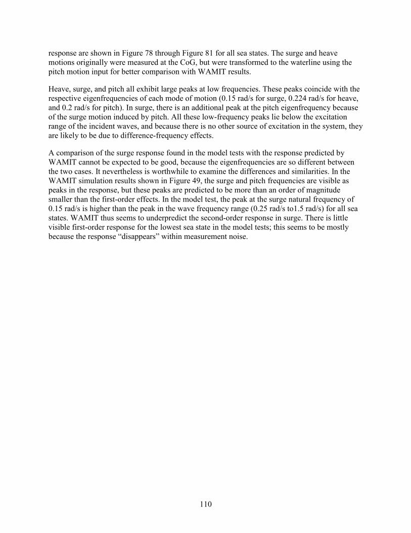
110
response are shown in Figure 78 through Figure 81 for all sea states. The surge and heave motions originally were measured at the CoG, but were transformed to the waterline using the pitch motion input for better comparison with WAMIT results.
Heave, surge, and pitch all exhibit large peaks at low frequencies. These peaks coincide with the respective eigenfrequencies of each mode of motion (0.15 rad/s for surge, 0.224 rad/s for heave, and 0.2 rad/s for pitch). In surge, there is an additional peak at the pitch eigenfrequency because of the surge motion induced by pitch. All these low-frequency peaks lie below the excitation range of the incident waves, and because there is no other source of excitation in the system, they are likely to be due to difference-frequency effects.
A comparison of the surge response found in the model tests with the response predicted by WAMIT cannot be expected to be good, because the eigenfrequencies are so different between the two cases. It nevertheless is worthwhile to examine the differences and similarities. In the WAMIT simulation results shown in Figure 49, the surge and pitch frequencies are visible as peaks in the response, but these peaks are predicted to be more than an order of magnitude smaller than the first-order effects. In the model test, the peak at the surge natural frequency of 0.15 rad/s is higher than the peak in the wave frequency range (0.25 rad/s to1.5 rad/s) for all sea states. WAMIT thus seems to underpredict the second-order response in surge. There is little visible first-order response for the lowest sea state in the model tests; this seems to be mostly because the response “disappears” within measurement noise.
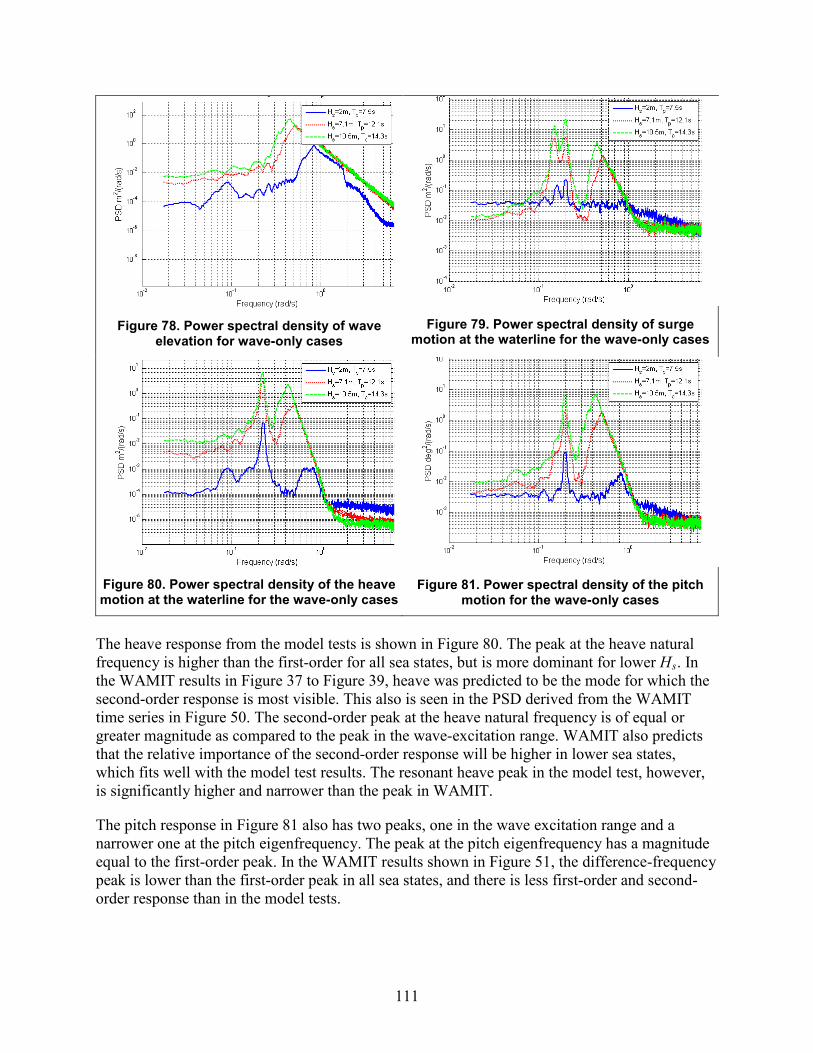
111
Figure 78. Power spectral density of wave
elevation for wave-only cases
Figure 79. Power spectral density of surge
motion at the waterline for the wave-only cases
Figure 80. Power spectral density of the heave motion at the waterline for the wave-only cases
Figure 81. Power spectral density of the pitch
motion for the wave-only cases
The heave response from the model tests is shown in Figure 80. The peak at the heave natural frequency is higher than the first-order for all sea states, but is more dominant for lower Hs. In the WAMIT results in Figure 37 to Figure 39, heave was predicted to be the mode for which the second-order response is most visible. This also is seen in the PSD derived from the WAMIT time series in Figure 50. The second-order peak at the heave natural frequency is of equal or greater magnitude as compared to the peak in the wave-excitation range. WAMIT also predicts that the relative importance of the second-order response will be higher in lower sea states, which fits well with the model test results. The resonant heave peak in the model test, however, is significantly higher and narrower than the peak in WAMIT.
The pitch response in Figure 81 also has two peaks, one in the wave excitation range and a narrower one at the pitch eigenfrequency. The peak at the pitch eigenfrequency has a magnitude equal to the first-order peak. In the WAMIT results shown in Figure 51, the difference-frequency peak is lower than the first-order peak in all sea states, and there is less first-order and second-order response than in the model tests.
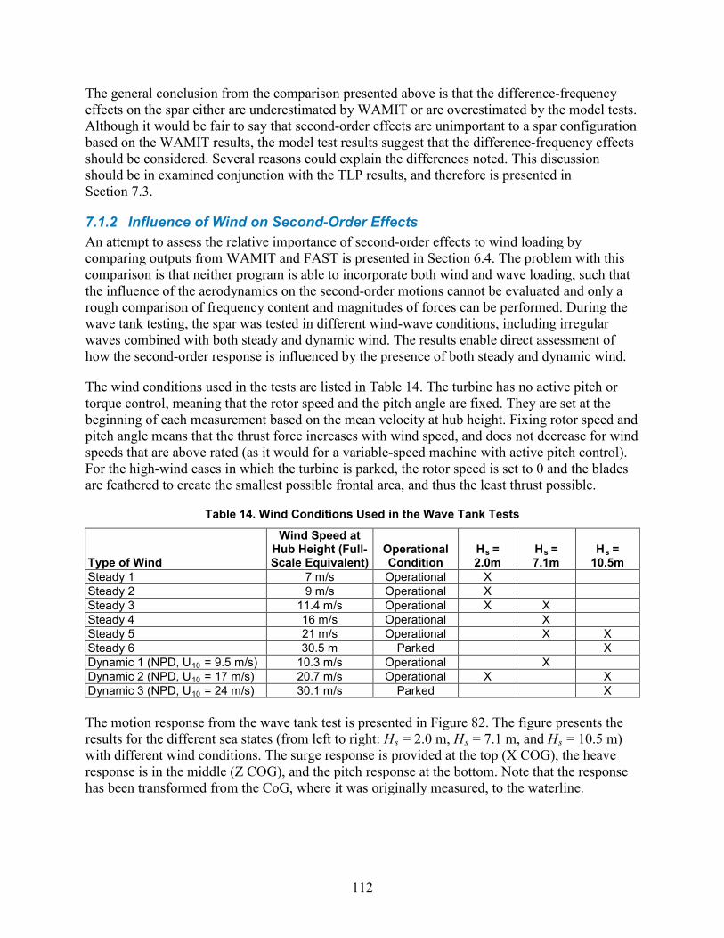
112
The general conclusion from the comparison presented above is that the difference-frequency effects on the spar either are underestimated by WAMIT or are overestimated by the model tests. Although it would be fair to say that second-order effects are unimportant to a spar configuration based on the WAMIT results, the model test results suggest that the difference-frequency effects should be considered. Several reasons could explain the differences noted. This discussion should be in examined conjunction with the TLP results, and therefore is presented in Section 7.3.
7.1.2 Influence of Wind on Second-Order Effects An attempt to assess the relative importance of second-order effects to wind loading by comparing outputs from WAMIT and FAST is presented in Section 6.4. The problem with this comparison is that neither program is able to incorporate both wind and wave loading, such that the influence of the aerodynamics on the second-order motions cannot be evaluated and only a rough comparison of frequency content and magnitudes of forces can be performed. During the wave tank testing, the spar was tested in different wind-wave conditions, including irregular waves combined with both steady and dynamic wind. The results enable direct assessment of how the second-order response is influenced by the presence of both steady and dynamic wind.
The wind conditions used in the tests are listed in Table 14. The turbine has no active pitch or torque control, meaning that the rotor speed and the pitch angle are fixed. They are set at the beginning of each measurement based on the mean velocity at hub height. Fixing rotor speed and pitch angle means that the thrust force increases with wind speed, and does not decrease for wind speeds that are above rated (as it would for a variable-speed machine with active pitch control). For the high-wind cases in which the turbine is parked, the rotor speed is set to 0 and the blades are feathered to create the smallest possible frontal area, and thus the least thrust possible.
Table 14. Wind Conditions Used in the Wave Tank Tests
Type of Wind
Wind Speed at Hub Height (Full-Scale Equivalent)
Operational Condition
Hs = 2.0m
Hs = 7.1m
Hs = 10.5m
Steady 1 7 m/s Operational X Steady 2 9 m/s Operational X Steady 3 11.4 m/s Operational X X Steady 4 16 m/s Operational X Steady 5 21 m/s Operational X X Steady 6 30.5 m Parked X Dynamic 1 (NPD, U10 = 9.5 m/s) 10.3 m/s Operational X Dynamic 2 (NPD, U10 = 17 m/s) 20.7 m/s Operational X X Dynamic 3 (NPD, U10 = 24 m/s) 30.1 m/s Parked X The motion response from the wave tank test is presented in Figure 82. The figure presents the results for the different sea states (from left to right: Hs = 2.0 m, Hs = 7.1 m, and Hs = 10.5 m) with different wind conditions. The surge response is provided at the top (X COG), the heave response is in the middle (Z COG), and the pitch response at the bottom. Note that the response has been transformed from the CoG, where it was originally measured, to the waterline.
113
The most important observations from the results are listed below.
• The first-order response (which is seen as a peak in the frequency range from 0.25 rad/s to 1 rad/s) is not significantly influenced by either steady or dynamic wind.
• Dynamic wind loading has the greatest influence on the low-frequency behavior and increases the response by several orders of magnitude, even for the 9 m/s case. Aerodynamics influences the low-frequency response more strongly when the turbine is operating than when it is not, as is shown by the two cases with the highest wind speeds.
• The cases in which the turbine is operating in high wind (such as 20 m/s dynamic wind or 21 m/s steady wind) influence the behavior at intermediate frequencies the most. The wind loading increases the response between the first-order and second-order peaks in surge and pitch.
• In the dynamic wind case in the lowest sea state, response induced by aerodynamic loading dominates at frequencies of less than 0.5 rad/s. The resonant peaks are still visible at the same frequency, but the magnitude is more than ten times greater. It is likely that the wind dominates the response to this extent because the wind is high (20 m/s at hub height) and the sea state is rather low (Hs = 2.0m).
• Subjecting the turbine to low to moderate steady winds does not significantly change the behavior, not even the mean offset. In pitch, the response peaks become a broader and a little lower with steady wind, and this also is seen in the pitch-induced surge response.
• The heave degree of freedom largely is unaffected by the wind, except for the dynamic-wind case in low sea.
The conclusions drawn from this analysis are that only dynamic wind provides any information about how the system reacts to aerodynamic loading, and not even the mean offset can be estimated based on steady wind. For heave, aerodynamics does not influence the response except if the wind speed is very great as compared to the wave height. In normal sea states, the wind potentially can be orders of magnitude more important than the wave loading, but as the severity of the sea state increases the influence of the wave loading also increases.
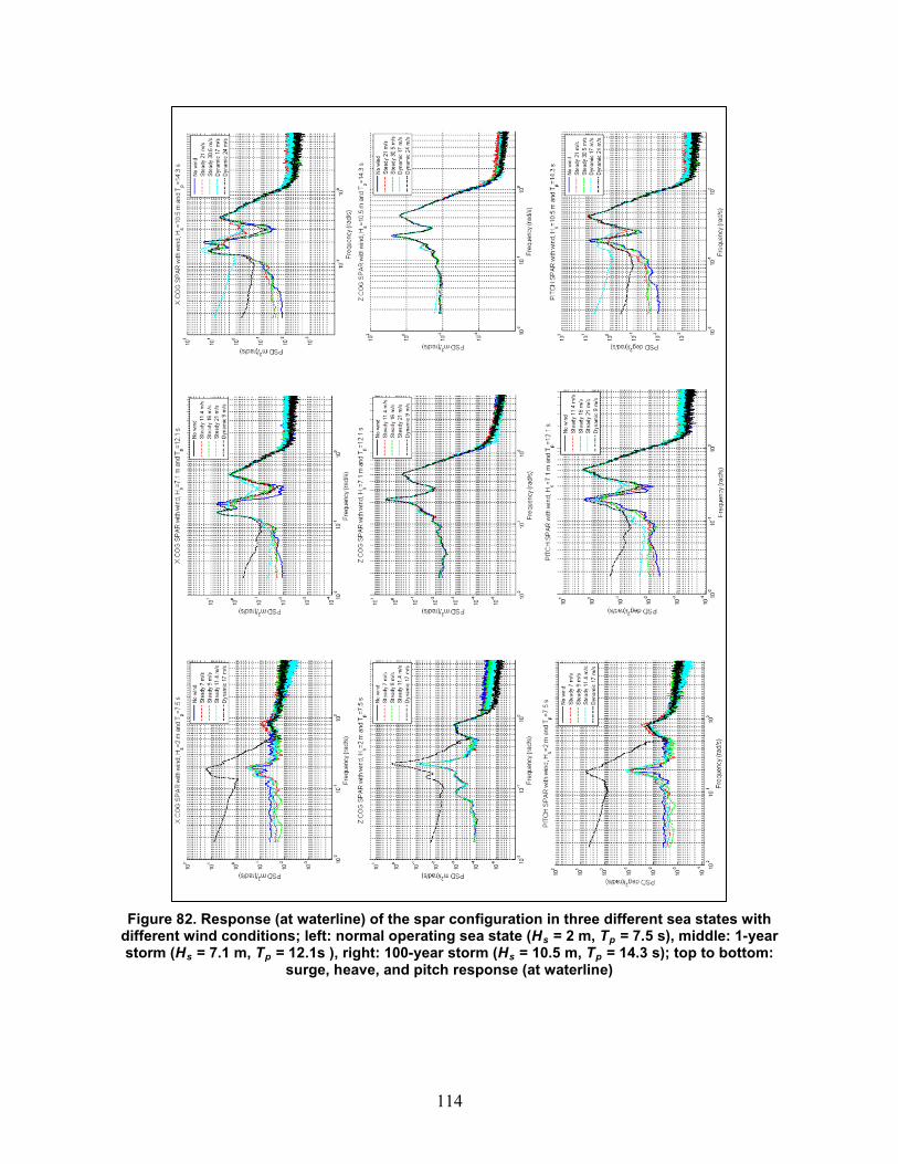
114
Figure 82. Response (at waterline) of the spar configuration in three different sea states with different wind conditions; left: normal operating sea state (Hs = 2 m, Tp = 7.5 s), middle: 1-year storm (Hs = 7.1 m, Tp = 12.1s ), right: 100-year storm (Hs = 10.5 m, Tp = 14.3 s); top to bottom:
surge, heave, and pitch response (at waterline)
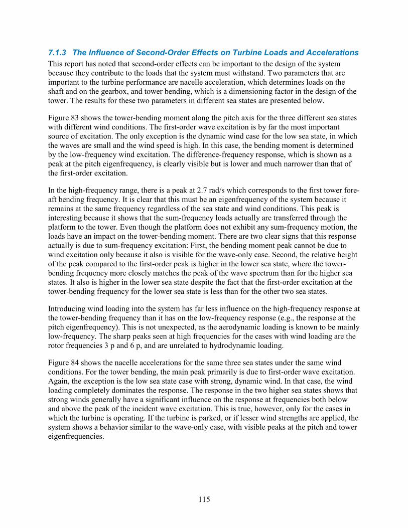
115
7.1.3 The Influence of Second-Order Effects on Turbine Loads and Accelerations This report has noted that second-order effects can be important to the design of the system because they contribute to the loads that the system must withstand. Two parameters that are important to the turbine performance are nacelle acceleration, which determines loads on the shaft and on the gearbox, and tower bending, which is a dimensioning factor in the design of the tower. The results for these two parameters in different sea states are presented below.
Figure 83 shows the tower-bending moment along the pitch axis for the three different sea states with different wind conditions. The first-order wave excitation is by far the most important source of excitation. The only exception is the dynamic wind case for the low sea state, in which the waves are small and the wind speed is high. In this case, the bending moment is determined by the low-frequency wind excitation. The difference-frequency response, which is shown as a peak at the pitch eigenfrequency, is clearly visible but is lower and much narrower than that of the first-order excitation.
In the high-frequency range, there is a peak at 2.7 rad/s which corresponds to the first tower fore-aft bending frequency. It is clear that this must be an eigenfrequency of the system because it remains at the same frequency regardless of the sea state and wind conditions. This peak is interesting because it shows that the sum-frequency loads actually are transferred through the platform to the tower. Even though the platform does not exhibit any sum-frequency motion, the loads have an impact on the tower-bending moment. There are two clear signs that this response actually is due to sum-frequency excitation: First, the bending moment peak cannot be due to wind excitation only because it also is visible for the wave-only case. Second, the relative height of the peak compared to the first-order peak is higher in the lower sea state, where the tower-bending frequency more closely matches the peak of the wave spectrum than for the higher sea states. It also is higher in the lower sea state despite the fact that the first-order excitation at the tower-bending frequency for the lower sea state is less than for the other two sea states.
Introducing wind loading into the system has far less influence on the high-frequency response at the tower-bending frequency than it has on the low-frequency response (e.g., the response at the pitch eigenfrequency). This is not unexpected, as the aerodynamic loading is known to be mainly low-frequency. The sharp peaks seen at high frequencies for the cases with wind loading are the rotor frequencies 3 p and 6 p, and are unrelated to hydrodynamic loading.
Figure 84 shows the nacelle accelerations for the same three sea states under the same wind conditions. For the tower bending, the main peak primarily is due to first-order wave excitation. Again, the exception is the low sea state case with strong, dynamic wind. In that case, the wind loading completely dominates the response. The response in the two higher sea states shows that strong winds generally have a significant influence on the response at frequencies both below and above the peak of the incident wave excitation. This is true, however, only for the cases in which the turbine is operating. If the turbine is parked, or if lesser wind strengths are applied, the system shows a behavior similar to the wave-only case, with visible peaks at the pitch and tower eigenfrequencies.
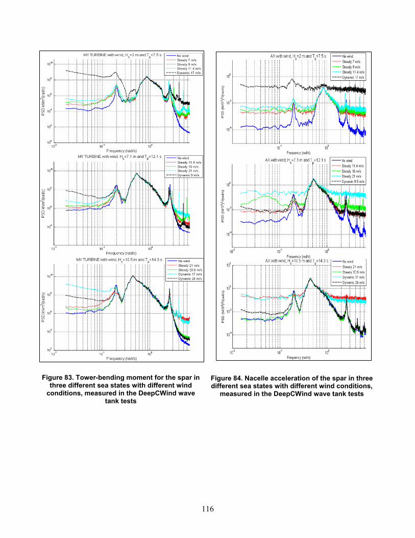
116
Figure 84. Nacelle acceleration of the spar in three different sea states with different wind conditions,
measured in the DeepCWind wave tank tests
Figure 83. Tower-bending moment for the spar in three different sea states with different wind
conditions, measured in the DeepCWind wave tank tests
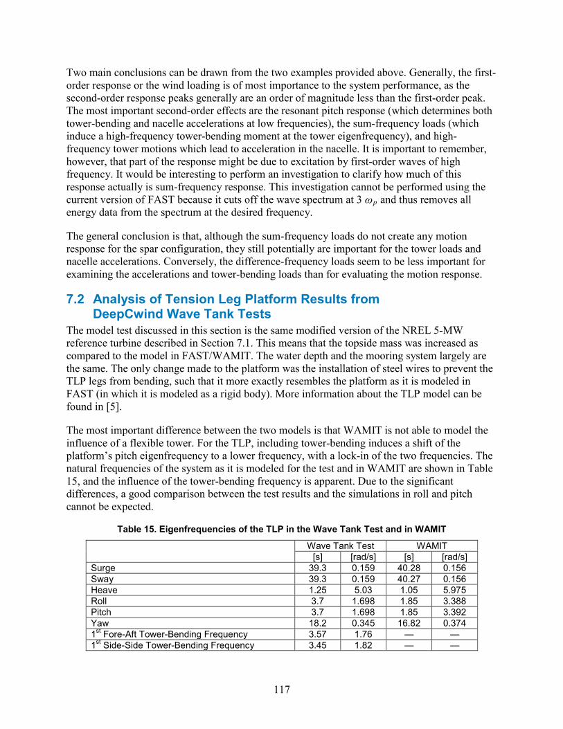
117
Two main conclusions can be drawn from the two examples provided above. Generally, the first-order response or the wind loading is of most importance to the system performance, as the second-order response peaks generally are an order of magnitude less than the first-order peak. The most important second-order effects are the resonant pitch response (which determines both tower-bending and nacelle accelerations at low frequencies), the sum-frequency loads (which induce a high-frequency tower-bending moment at the tower eigenfrequency), and high-frequency tower motions which lead to acceleration in the nacelle. It is important to remember, however, that part of the response might be due to excitation by first-order waves of high frequency. It would be interesting to perform an investigation to clarify how much of this response actually is sum-frequency response. This investigation cannot be performed using the current version of FAST because it cuts off the wave spectrum at 3 ωp and thus removes all energy data from the spectrum at the desired frequency.
The general conclusion is that, although the sum-frequency loads do not create any motion response for the spar configuration, they still potentially are important for the tower loads and nacelle accelerations. Conversely, the difference-frequency loads seem to be less important for examining the accelerations and tower-bending loads than for evaluating the motion response.
7.2 Analysis of Tension Leg Platform Results from DeepCwind Wave Tank Tests
The model test discussed in this section is the same modified version of the NREL 5-MW reference turbine described in Section 7.1. This means that the topside mass was increased as compared to the model in FAST/WAMIT. The water depth and the mooring system largely are the same. The only change made to the platform was the installation of steel wires to prevent the TLP legs from bending, such that it more exactly resembles the platform as it is modeled in FAST (in which it is modeled as a rigid body). More information about the TLP model can be found in [5].
The most important difference between the two models is that WAMIT is not able to model the influence of a flexible tower. For the TLP, including tower-bending induces a shift of the platform’s pitch eigenfrequency to a lower frequency, with a lock-in of the two frequencies. The natural frequencies of the system as it is modeled for the test and in WAMIT are shown in Table 15, and the influence of the tower-bending frequency is apparent. Due to the significant differences, a good comparison between the test results and the simulations in roll and pitch cannot be expected.
Table 15. Eigenfrequencies of the TLP in the Wave Tank Test and in WAMIT
Wave Tank Test WAMIT [s] [rad/s] [s] [rad/s]
Surge 39.3 0.159 40.28 0.156 Sway 39.3 0.159 40.27 0.156 Heave 1.25 5.03 1.05 5.975 Roll 3.7 1.698 1.85 3.388 Pitch 3.7 1.698 1.85 3.392 Yaw 18.2 0.345 16.82 0.374 1st Fore-Aft Tower-Bending Frequency 3.57 1.76 — — 1st Side-Side Tower-Bending Frequency 3.45 1.82 — —
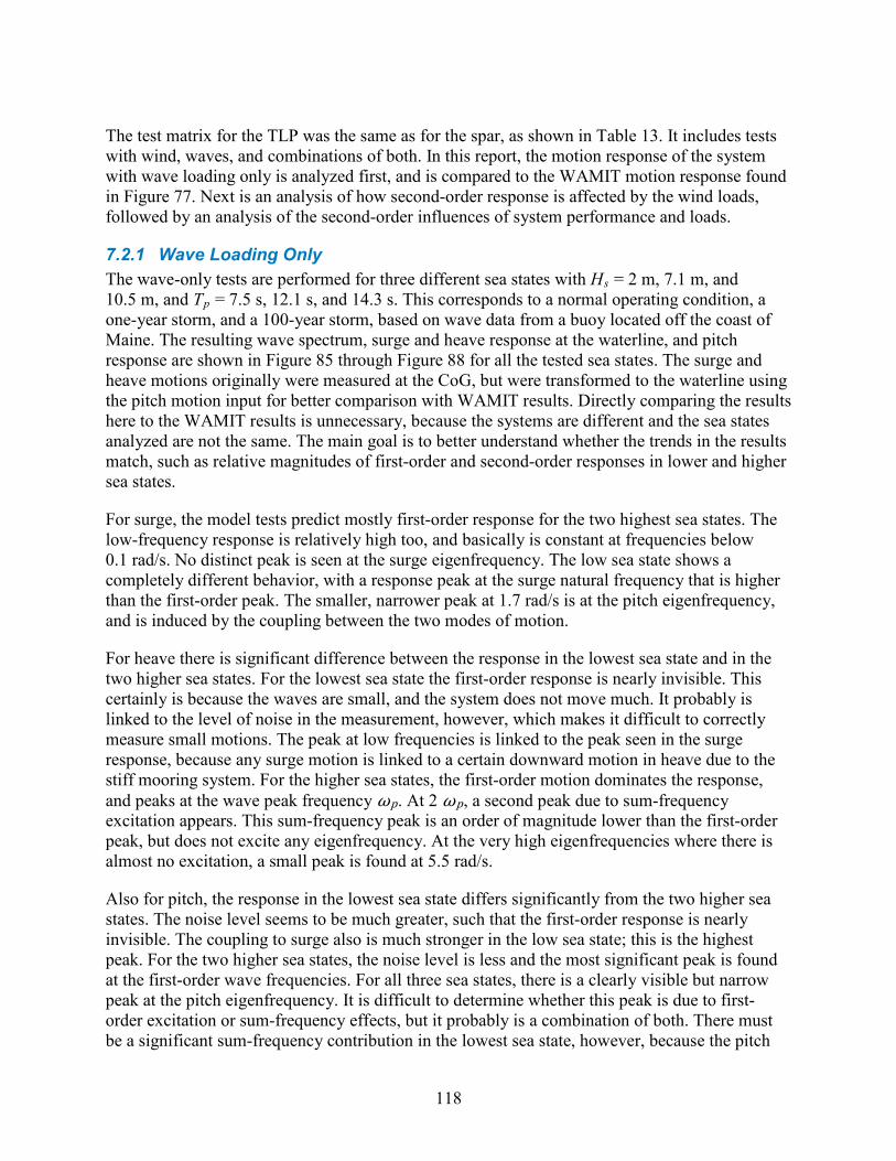
118
The test matrix for the TLP was the same as for the spar, as shown in Table 13. It includes tests with wind, waves, and combinations of both. In this report, the motion response of the system with wave loading only is analyzed first, and is compared to the WAMIT motion response found in Figure 77. Next is an analysis of how second-order response is affected by the wind loads, followed by an analysis of the second-order influences of system performance and loads.
7.2.1 Wave Loading Only The wave-only tests are performed for three different sea states with Hs = 2 m, 7.1 m, and 10.5 m, and Tp = 7.5 s, 12.1 s, and 14.3 s. This corresponds to a normal operating condition, a one-year storm, and a 100-year storm, based on wave data from a buoy located off the coast of Maine. The resulting wave spectrum, surge and heave response at the waterline, and pitch response are shown in Figure 85 through Figure 88 for all the tested sea states. The surge and heave motions originally were measured at the CoG, but were transformed to the waterline using the pitch motion input for better comparison with WAMIT results. Directly comparing the results here to the WAMIT results is unnecessary, because the systems are different and the sea states analyzed are not the same. The main goal is to better understand whether the trends in the results match, such as relative magnitudes of first-order and second-order responses in lower and higher sea states.
For surge, the model tests predict mostly first-order response for the two highest sea states. The low-frequency response is relatively high too, and basically is constant at frequencies below 0.1 rad/s. No distinct peak is seen at the surge eigenfrequency. The low sea state shows a completely different behavior, with a response peak at the surge natural frequency that is higher than the first-order peak. The smaller, narrower peak at 1.7 rad/s is at the pitch eigenfrequency, and is induced by the coupling between the two modes of motion.
For heave there is significant difference between the response in the lowest sea state and in the two higher sea states. For the lowest sea state the first-order response is nearly invisible. This certainly is because the waves are small, and the system does not move much. It probably is linked to the level of noise in the measurement, however, which makes it difficult to correctly measure small motions. The peak at low frequencies is linked to the peak seen in the surge response, because any surge motion is linked to a certain downward motion in heave due to the stiff mooring system. For the higher sea states, the first-order motion dominates the response, and peaks at the wave peak frequency ωp. At 2 ωp, a second peak due to sum-frequency excitation appears. This sum-frequency peak is an order of magnitude lower than the first-order peak, but does not excite any eigenfrequency. At the very high eigenfrequencies where there is almost no excitation, a small peak is found at 5.5 rad/s.
Also for pitch, the response in the lowest sea state differs significantly from the two higher sea states. The noise level seems to be much greater, such that the first-order response is nearly invisible. The coupling to surge also is much stronger in the low sea state; this is the highest peak. For the two higher sea states, the noise level is less and the most significant peak is found at the first-order wave frequencies. For all three sea states, there is a clearly visible but narrow peak at the pitch eigenfrequency. It is difficult to determine whether this peak is due to first-order excitation or sum-frequency effects, but it probably is a combination of both. There must be a significant sum-frequency contribution in the lowest sea state, however, because the pitch
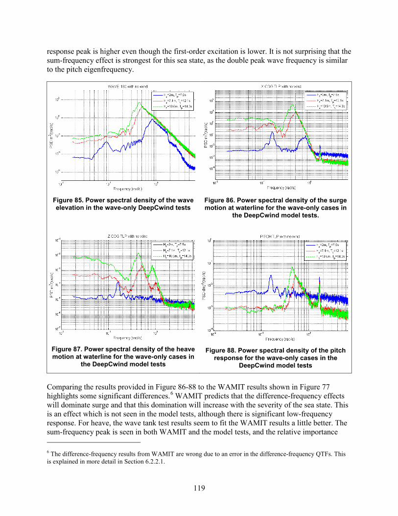
119
response peak is higher even though the first-order excitation is lower. It is not surprising that the sum-frequency effect is strongest for this sea state, as the double peak wave frequency is similar to the pitch eigenfrequency.
Figure 85. Power spectral density of the wave elevation in the wave-only DeepCwind tests
Figure 86. Power spectral density of the surge motion at waterline for the wave-only cases in
the DeepCwind model tests.
Figure 87. Power spectral density of the heave motion at waterline for the wave-only cases in
the DeepCwind model tests
Figure 88. Power spectral density of the pitch
response for the wave-only cases in the DeepCwind model tests
Comparing the results provided in Figure 86-88 to the WAMIT results shown in Figure 77 highlights some significant differences.6 WAMIT predicts that the difference-frequency effects will dominate surge and that this domination will increase with the severity of the sea state. This is an effect which is not seen in the model tests, although there is significant low-frequency response. For heave, the wave tank test results seem to fit the WAMIT results a little better. The sum-frequency peak is seen in both WAMIT and the model tests, and the relative importance 6 The difference-frequency results from WAMIT are wrong due to an error in the difference-frequency QTFs. This is explained in more detail in Section 6.2.2.1.
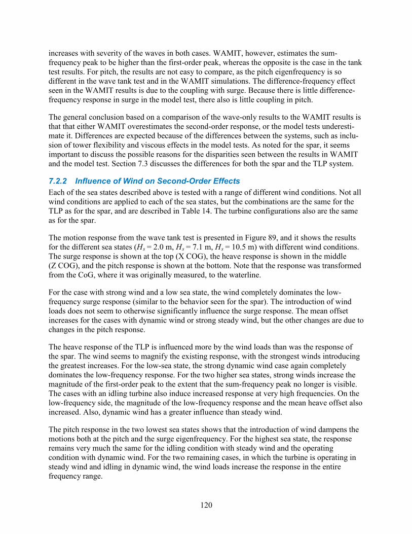
120
increases with severity of the waves in both cases. WAMIT, however, estimates the sum-frequency peak to be higher than the first-order peak, whereas the opposite is the case in the tank test results. For pitch, the results are not easy to compare, as the pitch eigenfrequency is so different in the wave tank test and in the WAMIT simulations. The difference-frequency effect seen in the WAMIT results is due to the coupling with surge. Because there is little difference-frequency response in surge in the model test, there also is little coupling in pitch.
The general conclusion based on a comparison of the wave-only results to the WAMIT results is that that either WAMIT overestimates the second-order response, or the model tests underesti-mate it. Differences are expected because of the differences between the systems, such as inclu-sion of tower flexibility and viscous effects in the model tests. As noted for the spar, it seems important to discuss the possible reasons for the disparities seen between the results in WAMIT and the model test. Section 7.3 discusses the differences for both the spar and the TLP system.
7.2.2 Influence of Wind on Second-Order Effects Each of the sea states described above is tested with a range of different wind conditions. Not all wind conditions are applied to each of the sea states, but the combinations are the same for the TLP as for the spar, and are described in Table 14. The turbine configurations also are the same as for the spar.
The motion response from the wave tank test is presented in Figure 89, and it shows the results for the different sea states (Hs = 2.0 m, Hs = 7.1 m, Hs = 10.5 m) with different wind conditions. The surge response is shown at the top (X COG), the heave response is shown in the middle (Z COG), and the pitch response is shown at the bottom. Note that the response was transformed from the CoG, where it was originally measured, to the waterline.
For the case with strong wind and a low sea state, the wind completely dominates the low-frequency surge response (similar to the behavior seen for the spar). The introduction of wind loads does not seem to otherwise significantly influence the surge response. The mean offset increases for the cases with dynamic wind or strong steady wind, but the other changes are due to changes in the pitch response.
The heave response of the TLP is influenced more by the wind loads than was the response of the spar. The wind seems to magnify the existing response, with the strongest winds introducing the greatest increases. For the low-sea state, the strong dynamic wind case again completely dominates the low-frequency response. For the two higher sea states, strong winds increase the magnitude of the first-order peak to the extent that the sum-frequency peak no longer is visible. The cases with an idling turbine also induce increased response at very high frequencies. On the low-frequency side, the magnitude of the low-frequency response and the mean heave offset also increased. Also, dynamic wind has a greater influence than steady wind.
The pitch response in the two lowest sea states shows that the introduction of wind dampens the motions both at the pitch and the surge eigenfrequency. For the highest sea state, the response remains very much the same for the idling condition with steady wind and the operating condition with dynamic wind. For the two remaining cases, in which the turbine is operating in steady wind and idling in dynamic wind, the wind loads increase the response in the entire frequency range.
121
Figure 89. Response of the TLP configuration in three different sea states with different wind conditions for (from left to right) normal operating sea state (Hs = 2 m, Tp = 7.5 s), 1-year storm
(Hs = 7.1 m, Tp = 12.1 s), and 100-year storm (Hs = 10.5 m, Tp = 14.3 s); and showing (from top to bottom) surge, heave, and pitch response (at waterline)
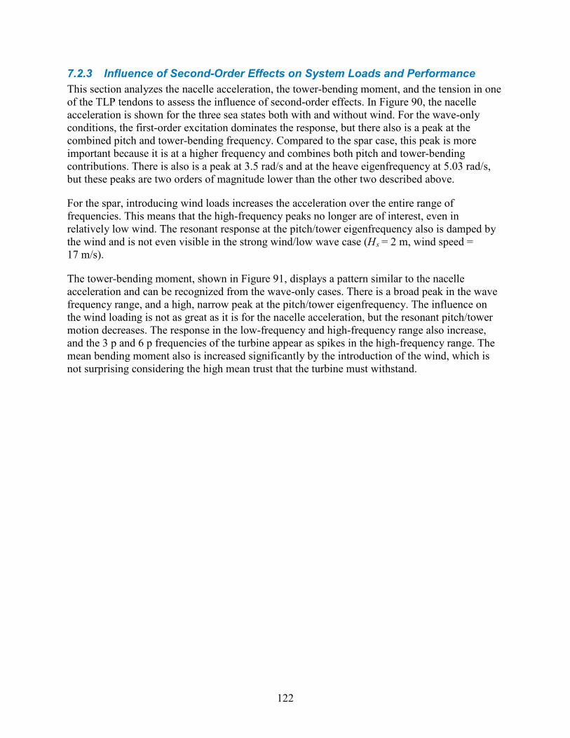
122
7.2.3 Influence of Second-Order Effects on System Loads and Performance This section analyzes the nacelle acceleration, the tower-bending moment, and the tension in one of the TLP tendons to assess the influence of second-order effects. In Figure 90, the nacelle acceleration is shown for the three sea states both with and without wind. For the wave-only conditions, the first-order excitation dominates the response, but there also is a peak at the combined pitch and tower-bending frequency. Compared to the spar case, this peak is more important because it is at a higher frequency and combines both pitch and tower-bending contributions. There is also is a peak at 3.5 rad/s and at the heave eigenfrequency at 5.03 rad/s, but these peaks are two orders of magnitude lower than the other two described above.
For the spar, introducing wind loads increases the acceleration over the entire range of frequencies. This means that the high-frequency peaks no longer are of interest, even in relatively low wind. The resonant response at the pitch/tower eigenfrequency also is damped by the wind and is not even visible in the strong wind/low wave case (Hs = 2 m, wind speed = 17 m/s).
The tower-bending moment, shown in Figure 91, displays a pattern similar to the nacelle acceleration and can be recognized from the wave-only cases. There is a broad peak in the wave frequency range, and a high, narrow peak at the pitch/tower eigenfrequency. The influence on the wind loading is not as great as it is for the nacelle acceleration, but the resonant pitch/tower motion decreases. The response in the low-frequency and high-frequency range also increase, and the 3 p and 6 p frequencies of the turbine appear as spikes in the high-frequency range. The mean bending moment also is increased significantly by the introduction of the wind, which is not surprising considering the high mean trust that the turbine must withstand.
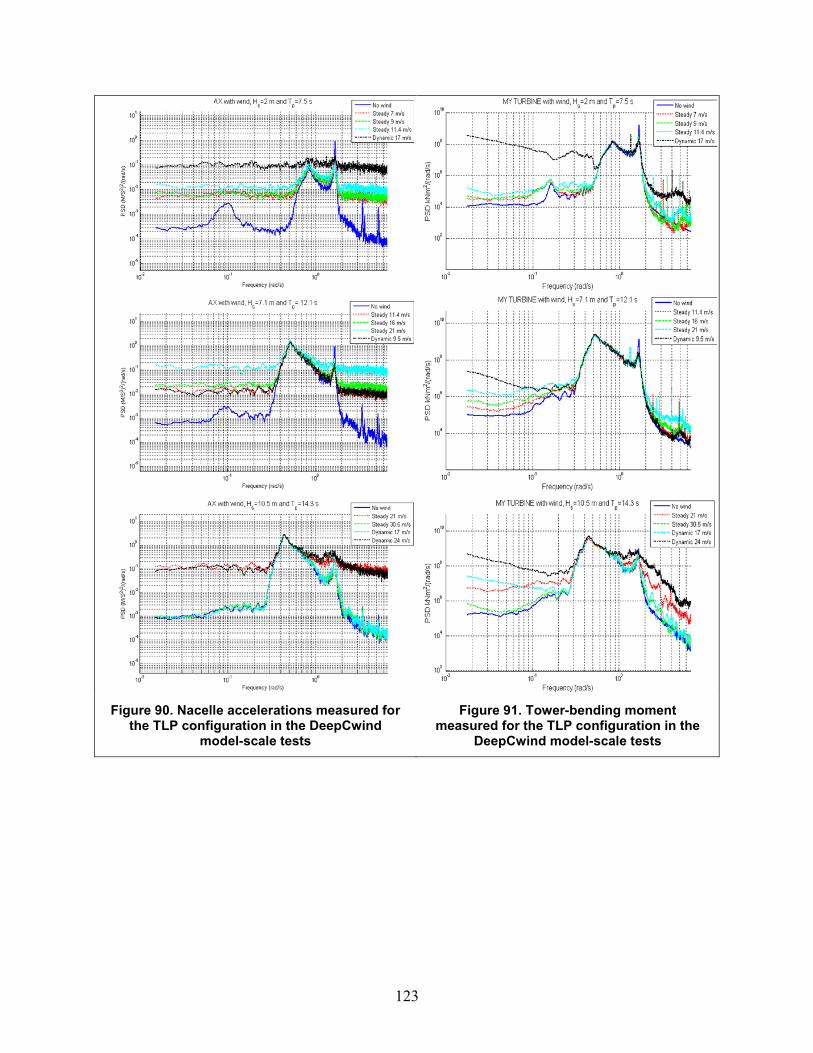
123
Figure 90. Nacelle accelerations measured for
the TLP configuration in the DeepCwind model-scale tests
Figure 91. Tower-bending moment measured for the TLP configuration in the
DeepCwind model-scale tests
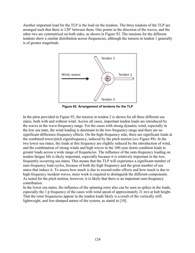
124
Another important load for the TLP is the load on the tendons. The three tendons of the TLP are arranged such that there is 120° between them. One points in the direction of the waves, and the other two are symmetrical on both sides, as shown in Figure 92. The tensions for the different tendons show a similar distribution across frequencies, although the tension in tendon 1 generally is of greater magnitude.
Figure 92. Arrangement of tendons for the TLP
In the plots provided in Figure 93, the tension in tendon 2 is shown for all three different sea states, both with and without wind. Across all cases, important tendon loads are introduced by the waves in the wave-frequency range. For the cases with strong dynamic wind, especially in the low sea state, the wind loading is dominant in the low-frequency range and there are no significant difference-frequency effects. On the high-frequency side, there are significant loads at the combined tower/pitch eigenfrequency, induced by the pitch motion (see Figure 89). In the two lower sea states, the loads at this frequency are slightly reduced by the introduction of wind, and the combination of strong winds and high waves in the 100-year storm condition leads to greater loads across a wide range of frequencies. The influence of the sum-frequency loading on tendon fatigue life is likely important, especially because it is relatively important in the low, frequently occurring sea states. This means that the TLP will experience a significant number of sum-frequency load cycles, because of both the high frequency and the great number of sea states that induce it. To assess how much is due to second-order effects and how much is due to high-frequency incident waves, more work is required to distinguish the different components. As noted for the pitch motion, however, it is likely that there is an important sum-frequency contribution. In the lower sea states, the influence of the spinning rotor also can be seen as spikes in the loads, especially the 1 p frequency of the cases with wind speed of approximately 21 m/s at hub height. That the rotor frequencies appear in the tendon loads likely is a result of the vertically stiff, lightweight, and low-damped nature of the system, as stated in [10].
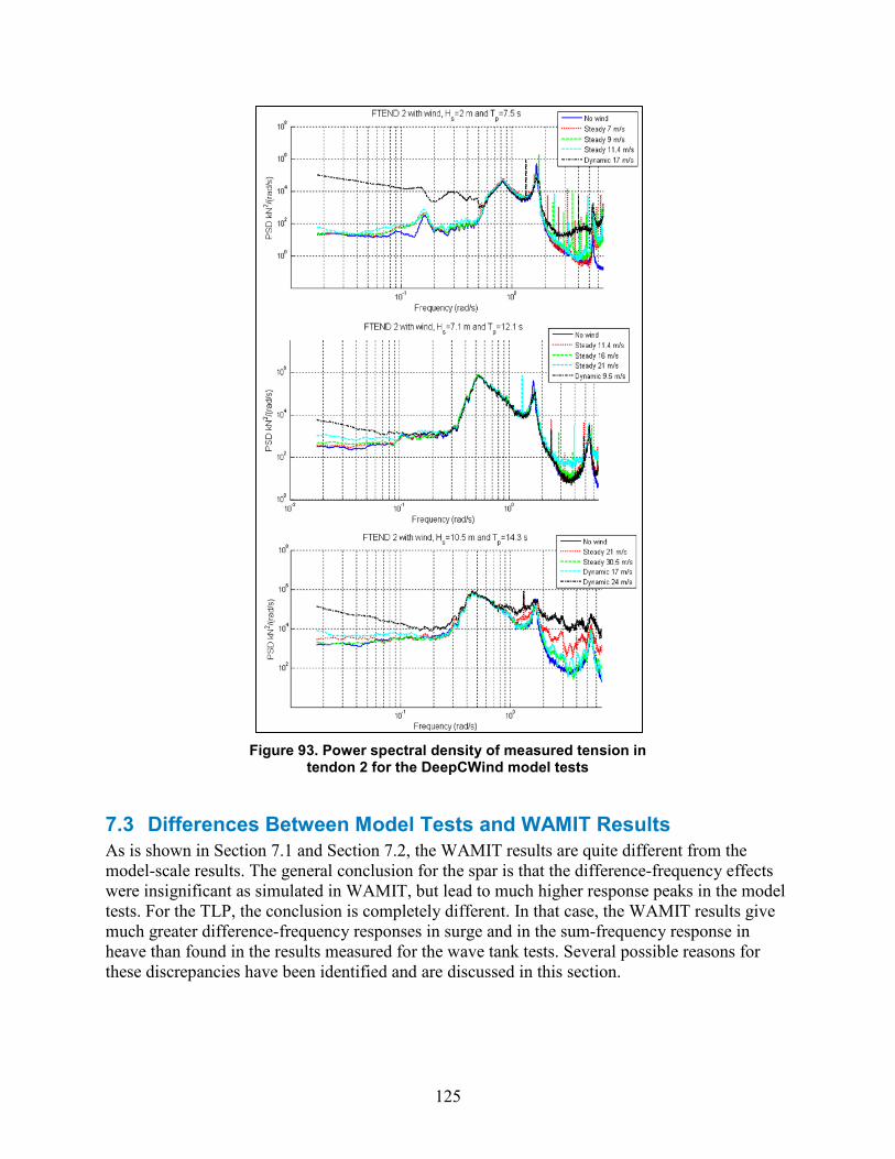
125
Figure 93. Power spectral density of measured tension in tendon 2 for the DeepCWind model tests
7.3 Differences Between Model Tests and WAMIT Results As is shown in Section 7.1 and Section 7.2, the WAMIT results are quite different from the model-scale results. The general conclusion for the spar is that the difference-frequency effects were insignificant as simulated in WAMIT, but lead to much higher response peaks in the model tests. For the TLP, the conclusion is completely different. In that case, the WAMIT results give much greater difference-frequency responses in surge and in the sum-frequency response in heave than found in the results measured for the wave tank tests. Several possible reasons for these discrepancies have been identified and are discussed in this section.
126
7.3.1 Differences in the System Dynamics The systems tested in the wave tank are different from the systems analyzed in WAMIT, as is noted in Section 7.1 and Section 7.2 for the spar and TLP, respectively. The mass of the turbine and rotor is increased by about 16% in the wave tank tests as compared to the reference turbine. The turbine tower is modeled including bending DOFs in the tank test, and the bending motion is very visible. For the spar, the water depth also is changed—from 320 in the WAMIT analysis to 200 m in the wave tank tests. Because of these changes the system dynamics change, with the shift of the eigenfrequencies being the most recognizable result.
For the spar, the surge eigenfrequency is changed from 0.05 rad/s in WAMIT to 0.15 rad/s in the tank test, mainly due to the change in the mooring system. The increased surge response in the tank test could be because the surge eigenfrequency is closer to the wave frequency range, such that there is possibly more or stronger excitation at 0.15 rad/s than 0.05 rad/s. This would fit well with the results observed for the difference-frequency force QTF provided in Figure 28, but does not explain the differences found for heave and pitch. The pitch motion of the system, however, is greatly influenced by the mass distribution—especially the mass high in the tower—so the increase in topside mass could have influenced the pitch results along with the introduction of a flexible tower. The heave is the result that seems to be most consistent across the tank test and the WAMIT analysis. This is reasonable in this context because heave is relatively independent of the mooring system, mass distribution, and tower flexibility.
For the TLP, the pitch eigenfrequency is shifted from 3.25 rad/s in WAMIT to 1.67 rad/s in the tank test. This means that the sum-frequency results for pitch are not at all comparable because the excitation of these two frequencies is so different.
7.3.2 Inaccuracies in the Model Test The system tested in the wave tank included some effects that are not representative of a full-scale system, and are even less representative for a system as it is modeled in WAMIT. The measurement cables used to record wind turbine data were rather heavy as compared to the system itself, as shown in Figure 94. The cables had a significant influence on the system motions and dynamics, as they started swinging when the turbine moved. This is the case for both the TLP and the spar. At this point, it is difficult to assess the significance of these cables.
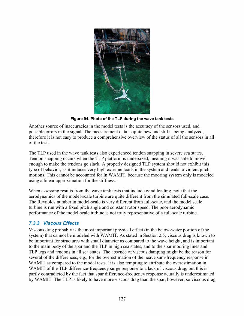
127
Figure 94. Photo of the TLP during the wave tank tests
Another source of inaccuracies in the model tests is the accuracy of the sensors used, and possible errors in the signal. The measurement data is quite new and still is being analyzed, therefore it is not easy to produce a comprehensive overview of the status of all the sensors in all of the tests.
The TLP used in the wave tank tests also experienced tendon snapping in severe sea states. Tendon snapping occurs when the TLP platform is undersized, meaning it was able to move enough to make the tendons go slack. A properly designed TLP system should not exhibit this type of behavior, as it induces very high extreme loads in the system and leads to violent pitch motions. This cannot be accounted for In WAMIT, because the mooring system only is modeled using a linear approximation for the stiffness.
When assessing results from the wave tank tests that include wind loading, note that the aerodynamics of the model-scale turbine are quite different from the simulated full-scale case. The Reynolds number in model-scale is very different from full-scale, and the model scale turbine is run with a fixed pitch angle and constant rotor speed. The poor aerodynamic performance of the model-scale turbine is not truly representative of a full-scale turbine.
7.3.3 Viscous Effects Viscous drag probably is the most important physical effect (in the below-water portion of the system) that cannot be modeled with WAMIT. As stated in Section 2.5, viscous drag is known to be important for structures with small diameter as compared to the wave height, and is important to the main body of the spar and the TLP in high sea states, and to the spar mooring lines and TLP legs and tendons in all sea states. The absence of viscous damping might be the reason for several of the differences, e.g., for the overestimation of the heave sum-frequency response in WAMIT as compared to the model tests. It is also tempting to attribute the overestimation in WAMIT of the TLP difference-frequency surge response to a lack of viscous drag, but this is partly contradicted by the fact that spar difference-frequency response actually is underestimated by WAMIT. The TLP is likely to have more viscous drag than the spar, however, so viscous drag
128
might at least be part of the explanation for the very high surge difference-frequency response produced by WAMIT.
It is possible to introduce an external damping matrix in WAMIT, which can be used to model the effective linear damping to capture the energy dissipation caused by viscous drag. Even if a linear approximation of the full scale drag had been added, however, the difference between the viscous forces in the numerical model and in the wave tank still would have been large. This is due to scaling issues related to the viscous effects—which are not particularly easy to resolve. Froude scaling is used for the waves, therefore the Reynolds number is not scaled correctly and the relative importance of viscous effects to inertia loads is distorted. As stated in [36], this is not so important when inertia-dominated structures are tested, but often creates difficulties for scaling the loads from model-scale to full-scale for drag-dominated structures. Compared to most oil platforms, the wind turbine structures have a small diameter. Therefore is rather questionable to assume that the forces are dominated by inertia forces, especially in the higher sea states. To mitigate the scaling error of the drag forces, models used for wave tank testing of slender structures typically are much greater than for structures that are dominated by inertia forces (e.g., scaling ratios of 1:20 instead of 1:50).
7.3.4 Inaccuracies in WAMIT Although there are many sources that make the model test results less reliable, the WAMIT results also contain inaccuracies. These include inaccuracies due to body discretization, the numerical representation of the hydrodynamic quantities, and inaccurate approximation of the instantaneous platform position during the calculation of second-order forces.
The second-order results consist of several contributions at one difference-frequency or sum-frequency. This raises the concern that inaccuracies are added together, such that tolerable inaccuracy levels become significant. If the spar QTFs are consistently underestimated (e.g., 95% of total), and the TLP QTFs are consistently overestimated (e.g., 105% of total), this could account for the “too low” spar results and the “too high” TLP results.
The most important parameter impacting the accuracy of the WAMIT results—the number of body panels—could not be properly tested for the TLP in the second-order convergence tests due to lack of computational power. The discretization used is similar to the typical discretizations found in literature and more refined than that used for the spar, but it is very difficult to assess the level of inaccuracy. The fact that second-order forces typically are assumed to be an order of magnitude less than the first-order forces provides reason to doubt the accuracy of the TLP QTFs computed by WAMIT. The TLP analyzed here, however, is orders of magnitude smaller than a TLP designed for use by the oil and gas industry. This raises the question whether “typical assumptions” apply at all.
7.3.5 Wave Representation One important possible source of differences between the simulation and the wave tank test results is the wave representation, as different wave spectra were used for the simulations and the wave tank tests. The wave spectrum used to derive the WAMIT time series was imported from FAST, to allow for a comparison of WAMIT time series to time series from FAST. The wave elevation from a WAMIT time series is shown in Figure 95, and the power spectral density of the wave elevation in the wave tank test is shown in Figure 96.
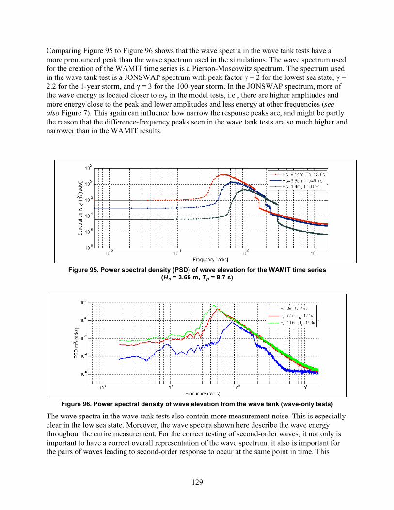
129
Comparing Figure 95 to Figure 96 shows that the wave spectra in the wave tank tests have a more pronounced peak than the wave spectrum used in the simulations. The wave spectrum used for the creation of the WAMIT time series is a Pierson-Moscowitz spectrum. The spectrum used in the wave tank test is a JONSWAP spectrum with peak factor γ = 2 for the lowest sea state, γ = 2.2 for the 1-year storm, and γ = 3 for the 100-year storm. In the JONSWAP spectrum, more of the wave energy is located closer to ωp in the model tests, i.e., there are higher amplitudes and more energy close to the peak and lower amplitudes and less energy at other frequencies (see also Figure 7). This again can influence how narrow the response peaks are, and might be partly the reason that the difference-frequency peaks seen in the wave tank tests are so much higher and narrower than in the WAMIT results.
Figure 95. Power spectral density (PSD) of wave elevation for the WAMIT time series (Hs = 3.66 m, Tp = 9.7 s)
Figure 96. Power spectral density of wave elevation from the wave tank (wave-only tests)
The wave spectra in the wave-tank tests also contain more measurement noise. This is especially clear in the low sea state. Moreover, the wave spectra shown here describe the wave energy throughout the entire measurement. For the correct testing of second-order waves, it not only is important to have a correct overall representation of the wave spectrum, it also is important for the pairs of waves leading to second-order response to occur at the same point in time. This
130
means that the wave spectrum must be correct not only across the whole measurement, but also for shorter periods within the measurement. If this requirement is not fulfilled, then the result could be an unrealistic (i.e., too high or too low) second-order response. The variation of the wave spectra and motion response spectra from the wave-tank tests with respect to time might lead to better understanding of whether this influenced the measurement results.
Another difference between the two wave representations is found at high wave frequencies. The wave spectrum as it is modeled in FAST is cut off at 3 ωp and thus eliminates potentially important first-order excitation at high frequencies. This cut-off frequency is shown in as a drop in the wave elevation PSD in Figure 95 and Figure 96. The cutoff is not as important for the spar, which exhibits very little response at high frequencies. For the TLP, which has significant low-frequency response, however, it can pose a problem. It does not heavily influence the simulation results from WAMIT seen in this report, because the eigenfrequencies of the system are far above the incident-wave frequency range in the WAMIT simulations. If the turbine is modeled with a flexible tower, however, then even a very small first-order wave at 2 rad/s can induce a significant motion response. An analysis of the first-order resonant response at high frequencies in FAST would be helpful for assessing how much of the high-frequency response is from first-order and second-order effects. Such an analysis only is possible if the wave spectrum is not cut off at too low a frequency.
7.3.6 Computation of Second-Order Results in WAMIT Another important issue requiring further investigation is the influence of the first-order RAOs on the second-order results. Both the second-order force contributions Fp and Fq depend on the first-order motions. The second-order potential force Fp also depends on the second-order scattering potential. The boundary-value problem for the scattering potential provided in Equation 2–61 through Equation 2–64 shows that the scattering potential depends on the forcing function B at the body boundary, which is given by Equation 2–64, and that B depends on the first-order motions. The dependence of the quadratic force Fq on the body motions easily is seen in Equation 2–71.
If WAMIT computes correct first-order RAOs, then there is no problem related to these formulations. This is normally the case if the structure above the water can be treated as a rigid body. If the body above the water is not rigid, however, then coupling effects can be important for the response. For the TLP—which has a high pitch frequency—it was noted that the tower-bending frequency and the pitch eigenfrequency mutually influence each other. In [27], the first-order RAOs were computed for a similar TLP system in WAMIT and in FAST with both a rigid and a flexible turbine. The results are shown for roll in Figure 97 (the results for other DOFs are similar). For the case with a rigid turbine, the results from WAMIT (red line) and FAST (blue line) are very similar, and especially the peaks are well aligned. If the turbine tower DOFs are included in the calculation in FAST, however, then the RAO changes significantly (black line). The peak is shifted to lower frequencies. The flexible tower cannot be modeled in WAMIT, therefore the second-order forces are calculated based on the wrong first-order motions.
The next step is to determine how important the inaccuracies of the first-order RAOs are to the second-order results. Of particular interest are the second-order forces, which are the input required for wind turbine simulations. For a system such as the TLP, which is very stiff in roll
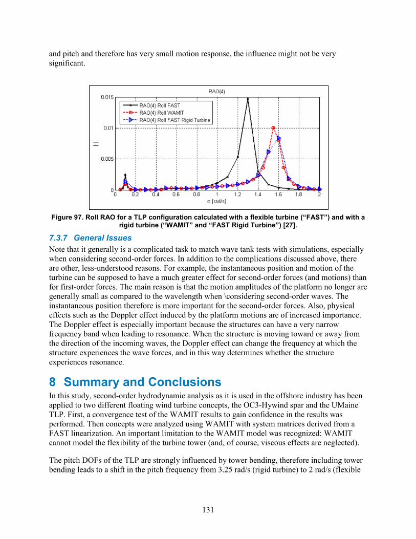
131
and pitch and therefore has very small motion response, the influence might not be very significant.
Figure 97. Roll RAO for a TLP configuration calculated with a flexible turbine (“FAST”) and with a rigid turbine (“WAMIT” and “FAST Rigid Turbine”) [27].
7.3.7 General Issues Note that it generally is a complicated task to match wave tank tests with simulations, especially when considering second-order forces. In addition to the complications discussed above, there are other, less-understood reasons. For example, the instantaneous position and motion of the turbine can be supposed to have a much greater effect for second-order forces (and motions) than for first-order forces. The main reason is that the motion amplitudes of the platform no longer are generally small as compared to the wavelength when \considering second-order waves. The instantaneous position therefore is more important for the second-order forces. Also, physical effects such as the Doppler effect induced by the platform motions are of increased importance. The Doppler effect is especially important because the structures can have a very narrow frequency band when leading to resonance. When the structure is moving toward or away from the direction of the incoming waves, the Doppler effect can change the frequency at which the structure experiences the wave forces, and in this way determines whether the structure experiences resonance.
8 Summary and Conclusions In this study, second-order hydrodynamic analysis as it is used in the offshore industry has been applied to two different floating wind turbine concepts, the OC3-Hywind spar and the UMaine TLP. First, a convergence test of the WAMIT results to gain confidence in the results was performed. Then concepts were analyzed using WAMIT with system matrices derived from a FAST linearization. An important limitation to the WAMIT model was recognized: WAMIT cannot model the flexibility of the turbine tower (and, of course, viscous effects are neglected).
The pitch DOFs of the TLP are strongly influenced by tower bending, therefore including tower bending leads to a shift in the pitch frequency from 3.25 rad/s (rigid turbine) to 2 rad/s (flexible
132
turbine). This problem, however, could not be solved within the time frame of this project, and the turbine only could be modeled as a rigid structure.
The frequency-domain results for the first-order and second-order hydrodynamic quantities such as added mass and damping coefficients, first-order force and motion RAOs, and second-order force and motion QTFs are presented and analyzed. Further, the frequency-domain results were used to generate time series that are compared with simulations that includes aerodynamic loads but no second-order excitation.
The test results from the DeepCwind model tests performed in a wave tank in Wageningen, Netherlands, next were analyzed to find second-order effects. The results first were compared with WAMIT results. The comparison showed that WAMIT underpredicts the second-order response of the spar, but overpredicts the second-order response of the TLP as compared to the model tests. Possible reasons for these differences are listed in Section 7, with the most important being the following.
• Differences in the systems, such as a rigid or flexible turbine, increased topside mass in the tank tests. Changes in the mooring system led to shifts in the surge eigenfrequency (for the spar) and in the pitch eigenfrequency (for the TLP). Additionally, the heavy measurement cables used in the wave tank test likely have an important effect on the system dynamics.
• Viscous effects that are present in the wave tank are not present in the WAMIT analysis. The viscous effects observed in the wave tank are not representative of a full-scale system because of scaling issues.
• Second-order results are based on inaccurate first-order motion RAOs in WAMIT.
• The wave representation differs between the simulations and the tests, with regard both to the chosen spectrum and the cut-off frequency.
Next, the model test results for the cases with combined wind and wave loading were analyzed to determine how the introduction of wind influences the second-order effects. The influence of second-order effects on tower-bending moment and nacelle accelerations also is analyzed. These all are parameters that cannot be analyzed with WAMIT, because WAMIT does not include aerodynamic loading and does not model the structure above the waterline.
Despite differences to WAMIT results and the uncertainties regarding error sources and scaling of viscous forces, some general conclusions can be drawn.
• For the OC3-Hywind spar, the peak values of the second-order QTFs from WAMIT are at least an order of magnitude smaller than the peak values for first-order QTFs.
• The difference-frequency response at the eigenfrequencies is the most important second-order effect for the spar, and is the most significant relative to the first-order response for heave. This is a result that is obtained both from the model tests and from WAMIT. The difference-frequency response is more significant in the model tests, however, than in WAMIT for all degrees of freedom.
133
• For the UMaine TLP, the second-order force QTFs from WAMIT peak at about 50% of the first-order peak, which means that they are much more significant than for the spar.7 This also influences the response calculated by WAMIT, which show high difference-frequency response in surge with a coupling to pitch and significant non-resonant sum-frequency response in heave.
• In the TLP model tests, there is no significant peak in the surge response at the surge eigenfrequency although the low-frequency response is quite high. In heave, non-resonant response from sum-frequency forces is seen, but it is much less than found in WAMIT, probably due to viscous damping. The pitch response cannot be compared between WAMIT and the model test because the eigenfrequencies of the two systems are so different. There is, however, sum-frequency response at the pitch eigenfrequency in the model tests, although it is not very significant.
• Mean-drift forces computed in WAMIT are very small as compared to aerodynamic thrust from FAST, and therefore can be viewed as insignificant (less than 1% of the mean thrust) as long as the turbine is operating. If the turbine is idling, then the relative significance of the mean-drift forces increases, but they never comprise more than about 15% of the mean thrust force (even without including aerodynamic forces due to tower drag). This behavior is confirmed by the wave tank tests, in which dynamic wind increases the mean offset of the turbine by several orders of magnitude.
• The PSD of rotor thrust time series and surge response time series from FAST show that aerodynamics induces significant low-frequency loads and responses. This means that the difference-frequency effects are likely to be unimportant in comparison. The wave tank test confirmed this. In a low sea state with high wind (e.g., Hs = 2 m, wind speed at hub height = 21 m/s), the low-frequency response below 0.5 rad/s is completely dominated by aerodynamics. High aerodynamic loading also increases the motion response at high frequencies, and tends to decrease the importance of sum-frequency peaks.
• For the TLP, the sum-frequency response in pitch is considered the most important second-order effect because of the coupling between the pitch and tower eigenfrequency. This also is important because sum-frequency pitch motions translate into nacelle accelerations and tower-bending moments, and also have a significant effect on the tendon loads. This means that care is required for choosing the pitch eigenfrequency, and ideally it should be designed to be at a higher frequency than in the model tests, further away from the wave-frequency range.
• For the spar, the sum-frequency loads were found to be translated to the tower even though they do not induce any pitch motion. The sum-frequency loads excite the tower-bending frequency and, as such, induce a tower-bending moment and nacelle accelerations.
No clear conclusion about whether second-order effects are important to the design of a turbine can be determined from the analysis presented. Difference-frequency effects seem to induce
7 The difference-frequency results calculated based on WAMIT output are affected by the error in the QTF calculation, as described in Section 6.2.2.1. This error is significant enough that the difference-frequency results for the TLP cannot be trusted.
134
possibly large response, but most often probably will be dominated by aerodynamics. Sum-frequency excitation is important to platform motions when the eigenfrequency is just above the incident wave range, but also can excite tower bending in other systems. The main outcome of this work is presenting a method for analyzing the second-order effects of a wind turbine, and simultaneously examining limitations to this method. The most important conclusion probably is that the type of analysis used for large offshore oil platforms is not necessarily directly applicable to the typically much smaller wind turbine structures. Further, a great number of results have been presented. Although the results are not easy to interpret, it is hoped that they can form a basis for future work.
9 Recommendations for Future Work If second-order hydrodynamics were implemented in FAST, it then would be a valuable tool for further analysis of the second-order effects. It would allow for modeling of the turbine as a flexible body, and the influence of second-order effects on the overall turbine loads would be easier to analyze as they could be calculated both alone and in combination with first-order loads. These results then could be compared to simulations that include only first-order loads. Further, FAST could be used to assess the effect of second-order hydrodynamics for a much wider range of different environmental conditions than is possible in model tests.
Before this can be done, however, some problems must be resolved. Most importantly, the accuracy of the method used to calculate second-order results in WAMIT must be assessed. A possible way to determine the influence of the first-order RAO on the second-order forces might be to create two systems with the same geometry, but with different mass and external damping/stiffness matrices. These two systems would experience the same first-order loads, but would have different first-order RAOs. This would lead to differences in the second-order loads that only are due to the differences in the first-order motions. If the differences are significant, then the next question would whether there is a way to include tower bending in WAMIT, or a way to import correct first-order motion response to WAMIT.
There also are many steps that can be taken to better understand the differences between the model tests and WAMIT. One possibility would be to rerun the WAMIT cases with additional damping that is adjusted to the damping in the wave tank test, as presented in Goupee et al. (2012b). If WAMIT is rerun, then the FAST models that are under development as part of the DeepCwind project could be used to get the linearized system matrices. These FAST models are meant to match the turbine models tested in the tank best as is possible, but were not available at the time of this work. Throughout the process of matching the FAST model to the model-test results, the understanding of the model test will also be increased and perhaps lead to new insight about why test results differ so widely between WAMIT and the wave tank. Moreover, full-scale floating-turbine data from the pilot projects would be very valuable for increasing the understanding of the influence of second-order effects.
This work only is the beginning of a complete assessment of second-order effects. Many parameters influence the second-order effects, such as water depth, short- or long-crestedness of the sea state, and the size (i.e., diameter) of the structure. It is important that future work assess the influence of these parameters, for example if the turbine was scaled from 5 MW to 10 MW. A structure with several columns, such as the semi-submersible tested in the DeepCwind tests,

135
also can experience interaction effects that increase the effect of the second-order loads. The impact of second-order effects on extreme loads and fatigue for a wide range of turbine configurations must be understood before a conclusion can be drawn about whether these effects are important.
References [1] AeroHydro Inc (2012), “MultiSurf for WAMIT 8.0.”, AeroHydro Inc. Accessed April 14,
2013: http://www.aerohydro.com/tutorials.htm [2] Agarwal, P. (2008). Simulation Structural Reliability Offshore Wind Turbines. Ph.D.
Dissertation. Austin, TX: University of Texas at Austin. [3] Bir, G. (October 2008). User’s Guide to MBC3 (Draft). Golden, CO: National Renewable
Energy Laboratory. Accessed April 14, 2013: http://wind.nrel.gov/designcodes/ postprocessors/mbc/.
[4] Det Norske Veritas (2007). Recommended Practice DNV RP-C205 Environmental Conditions and Environmental Loads. Høvik, Norway: Det Norske Veritas.
[5] de Ridder, E.J.; Koop, A.H.; Doeveren, A.G. (December 2011). DeepCwind Floating Wind Turbine Model Tests. Report No. 24602-1-OB. Wageningen, Netherland: Maritime Research Institute (MARIN).
[6] Eatock Taylor, R.; Natvig, B. J. (1994). “Effect of Wave Drift Damping on TLP Horizontal Offsets.” Prepared for BOSS ’94, 7th Int’l Conf. on the Behaviour of Offshore Structures, July 12–15, 1994. Boston, MA: MIT.
[7] European Wind Energy Association (2012). Accessed February 2012: www.ewea.org. [8] Faltinsen, O. M. (1990). Sea Loads on Ships and Offshore Structures. Cambridge, UK:
Cambridge University Press. [9] Goupee, A.J.; Koo, B.; Kimball, R.W.; Lambrakos, K.F. (2012a). “Experimental
Comparison of Three Floating Wind Turbine Concepts.” Proceedings of the 31st International Conference on Ocean, Offshore and Arctic Engineering; June 10–15, 2012, Rio de Janeiro, Brazil
[10] Goupee, A.J.; Koo, B.; Lambrakos, K.F.; Kimball, R.W. (2012b). “Offshore Wind Energy: Model Tests for Three Floating Wind Turbine Concepts.” Proceedings of the Offshore Technology Conference; April 30 to May 3, 2012, Houston, TX.
[11] International Electrotechnical Commission (IEC 2009). IEC 61400–3. 1st edition. “Wind Turbines—Part 3: Design Requirements for Offshore Wind Turbines.” Geneva, Switzerland: International Electrotechnical Commission
[12] “IEA Energy Statistics—Renewables and Waste in World in 2009.” (2012). International Energy Agency. Accessed April 14, 2013: http://www.iea.org/stats/renewdata.asp? COUNTRY_CODE =29.
[13] Jonkman, B. (2009). TurbSim User’s Guide: Version 1.50. NREL/TP-500-46198. Golden, CO: National Renewable Energy Laboratory.
[14] Jonkman, J. (2010). Definition of the Floating System for Phase IV of OC3. NREL/TP-500- 47535. Golden, CO: National Renewable Energy Laboratory. Accessed April 14, 2013: www.nrel.gov/docs/fy10osti/47535.pdf.
[15] Jonkman, J. (2007). Dynamics Modeling and Loads Analysis of an Offshore Floating Wind Turbine. Ph.D. Thesis. NREL/TP-500-41958. Golden, CO: National Renewable Energy Laboratory. Accessed April 14, 2013: www.nrel.gov/docs/fy08osti/41958.pdf.

136
[16] Jonkman, J. M.; Buhl, M. L., Jr. (2005). FAST User’s Guide. NREL/EL-500-38230. Golden, CO: National Renewable Energy Laboratory. Accessed April 14, 2013: wind.nrel.gov/designcodes/simulators/fast/FAST.pdf.
[17] Jonkman, J.; Butterfield, S.; Musial, W.; Scott, G. (2009). Definition of a 5-MW Reference Wind Turbine for Offshore System Development. NREL/TP-500-38060. Golden, CO: National Renewable Energy Laboratory. Accessed April 14, 2013: www.nrel.gov/docs/fy09osti/38060.pdf .
[18] Jonkman, J., NREL Wind Turbine Modelling Workshop, National Renewable Energy Laboratory, March 2nd, 2012 https://wind.nrel.gov/forum/wind/viewtopic.php?f=4&t=589
[19] Kim, M.-H.; Yue, D.K.P. (1990a). “The Complete Second-Order Diffraction Solution for an Axisymmetric Body. Part 1. Monochromatic Incident Waves.” J. Fluid Mech. (200); pp. 235–264.
[20] Kim, M.-H.; Yue, D.K.P. (1990b). “The Complete Second-Order Diffraction Solution for an Axisymmetric Body. Part 2. Bichromatic Incident Waves and Body Motions.” J. Fluid Mech. (211), pp. 557–593.
[21] Krokstad, J.R.; Stansberg, C.T.; Nestegård, A.; Marthinsen, T. (1996). “A New Non-Slender Ringing Load Approach Verified Against Experiments.” 15th OMAE Conference, Florence .
[22] Kvitrud, A. (2012). “Høyere Ordens Lastvirkninger (Ringing and Springing).” Accessed April 2, 2013: http://home.online.no/~akvitrud/ringing-status-1994.htm .
[23] Lee, C.-H. (1995). WAMIT Theory Manual. Cambridge, MA: MIT. Accessed April 14, 2013: www.wamit.com/Publications/tmanual.pdf .
[24] Lee, C.-H.; Newman, J.N. (2005). “Computation of Wave Effects Using the Panel Method.” Preprint, in Chakrabart, S.K., Numerical Models in Fluid-Structure Interaction, WAMIT Inc. Accessed April 14, 2013: www.wamit.com/Publications/wit2003.pdf .
[25] Lewis, E.V. ed. (1988). Principles of Naval Architecture (Second Revision). “Volume II. Resistance, Propulsion and Vibration., Society of Naval Architects and Marine Engineers (SNAME).
[26] Lucas, J. (2011). UpWind Project: Comparison of a First- and Second-Order Hydrodynamic Results for Floating Offshore Wind Structures. Bristol, UK: Garrad Hassan & Partners Ltd.
[27] Matha, D. (2010). Model Development and Loads Analysis of an Offshore Wind Turbine on a Tension Leg Platform, with a Comparison to Other Floating Turbine Concepts. NREL/SR-500-45891. Golden, CO: National Renewable Energy Laboratory. Accessed April 14, 2013: www.nrel.gov/docs/fy10osti/45891.pdf .
[28] Moriarty, D.J.; Hansen, A.C. (2005). AeroDyn Theory Manual. NREL/EL-500-36881. Golden, CO: National Renewable Energy Laboratory. Accessed April 14, 2013: wind.nrel.gov/designcodes/simulators/aerodyn/AD_Theory.pdf .
[29] Musial, W.; Ram, B. (2010). Large Scale Offshore Wind Power in the United States. NREL/TP-500-40745. Golden, CO: National Renewable Energy Laboratory. Accessed April 14, 2013: www.nrel.gov/wind/pdfs/40745.pdf .
[30] National Data Buoy Center (NDBC 2013). http://www.ndbc.noaa.gov/ (accessed April 3, 2013).
[31] National Wind Technology Center (NWTC 2013). Simulation code download available at http://wind.nrel.gov/designcodes/simulators/ (accessed April 3, 2013).
137
[32] Nielsen, F. G. (1996). “Hydrodynamics in Industry. Some Examples with Special Emphasis on Marine Applications.” Grue, J.; Gjevik, B.; Weber, J.E. Eds. Waves and Nonlinear Processes in Hydrodynamics Series: Fluid Mechanics and Its Applications. The Netherlands: Kluwer Academic Publishers.
[33] Newman, J.N. (1992). “Sensitivity of Wave Loads to the Discretization of Bodies.” Prepared for BOSS ’92, 6th Int’l Conference on the Behaviour of Offshore Structures, July 7–10, 1992. London, U.K.: BPP Tech Services Ltd. pp. 50–64.
[34] Newman, J.N. (1977). Marine Hydrodynamics. Cambridge, MA: MIT Press. [35] Orcina Ltd. (2013). OrcaFlex Manual. Daltongate, Cumbria, UK: Orcina Ltd. Accessed
April 3, 2013: http://www.orcina.com/SoftwareProducts/OrcaFlex/Documentation/ index.php .
[36] Petterson, B. (August 1993). Hydrodynamikk og havmiljø grunnkurs, Del III: Bølgekrefter (foreløpig utgave). Faculty of Marine Technology, Norwegian University of Science and Technology, NTNU–Trondheim.
[37] Robertson, A.N.; Jonkman, J.M. (2011). “Loads Analysis of Several Offshore Floating Wind Turbine Concepts.” Proceedings of the Twenty-First (2011) International Offshore and Polar Engineering Conference; June 19–24, 2011, Maui, Hawaii.
[38] Stansberg, C.T. (1997). “Comparing Ringing Loads from Experiments with Cylinders of Different Diameters—An Empirical Study.” BOSS, Int’l Conference on the Behaviour of Offshore Structures. Delft: The Netherlands.
[39] Stansberg, C.T. (1993). “Statistical Properties of Nonlinear Wave-Induced High Frequency Responses in Random Waves.” Prepared for Tension Buoyant Platforms Seminar, May 25–26, 1993, London, UK.
[40] Triantafyllou, M.S. and Chryssostomidis, C., Lecture notes [41] WAMIT, Inc. (2002). WAMIT User Manual, Version 6.4., WAMIT Inc. [42] World Wind Energy Association (2012). Accessed February 2012:
http://www.wwindea.org.
138
Appendix: FAST Linearization Process To solve the equations of motion, WAMIT requires information about inertia, damping, and stiffness. If the body is floating freely, then the only necessary input are the radii of gyration and the vertical position of the center of gravity (CoG). In this case, it is assumed that the CoG lies along the line where X = Y =0. If a wind turbine is mounted atop the platform, then the CoG generally is not at X= Y = 0, due to the rotor and nacelle overhang. If the CoG offset is to be taken into account, then a different input format must be used. In this format, the full (X, Y, Z) position of the CoG must be specified, and the full 6 x 6 mass matrix be defined. It also is possible to define 6 x 6 external stiffness and damping matrices to take into account damping and stiffness in the system that are not produced by solving the hydrodynamics/hydrostatics problem for the platform geometry in WAMIT. For a wind turbine, this includes contributions from aerodynamics, rotor gyroscopics, and the mooring system.
To find the system matrices, a model of the wind turbine in FAST is linearized around an operating point, and the outputs are post-processed in MatLab. It is important to understand how FAST uses the hydrodynamic input from WAMIT in the linearization process, such that all effects are included but none are counted twice. The process involves several steps and exchanges of inputs between FAST and WAMIT.
To run FAST for a floating platform, inputs from WAMIT are required to account for hydrodynamics. These inputs include hydrodynamic restoring (“.hst” file), added mass and damping (“.1” file), and wave excitation forces (“.3” file). FAST accounts for the gravity terms of the hydrodynamic restoring internally, therefore these terms must not be included in the “.hst” file. The simplest way to avoid this is by setting the vertical CoG position to zero in WAMIT. When doing this, it is important to remember that the RAOs computed by WAMIT will be incorrect (unless the CoG position actually is 0). The OC3-Hywind directory and other floating wind turbine directories that can be downloaded from the National Wind Technology Center (NWTC) homepage include the WAMIT output files derived in the described fashion, so it is not necessary to run WAMIT to be able to perform FAST analysis or linearization for these turbines.
To obtain the mass, damping, and stiffness inputs required to run WAMIT, a second-order linearization of the model in FAST is run for the operating point of interest. The only DOFs included are the platform DOFs surge, sway, heave, roll, pitch, and yaw. As the aerodynamic inertia, damping, and stiffness change with changing wind conditions, it is important to choose the correct operating point.
It is not possible to linearize FAST with wave radiation damping or time-varying wave excitation, therefore these effects must be turned off in the FAST linearization (RdtnTMax = 0.0 to turn off wave radiation; WaveMod = 0 to turn off all wave excitation). To eliminate damping contributions from viscous drag, the viscous drag can be removed from the linearization by setting the drag coefficient PtfmCD to zero. Rotor gyroscopics can be turned off by setting the rotor speed to zero. It also is important to use the right FAST executable, which means not using the executable specifically designed for the OC3-Hywind (because this includes additional damping). After the linearization is run in FAST, the postprocessing MatLab file “GetMats.m” that is provided with MBC3 should be run, as described in [3].
139
The output from the linearization is as follows:
• the stiffness matrix, including hydrodynamic restoring (with gravity terms)
• the damping matrix, without wave radiation damping
• the mass matrix, including the infinite frequency added mass. From this output, the damping matrix can be used directly. The mass matrix must be postprocessed, that is, the added mass matrix at the infinite frequency limit A∞ must be subtracted from the mass matrix. The best way of doing this is by using the same A∞ that was sent to FAST from WAMIT. The stiffness matrix also must be postprocessed and—because this is a special case—is explained more thoroughly here.
The stiffness matrix K has many different contributions as seen in Equation A–1.
𝐾𝑡𝑜𝑡𝑎𝑙 = 𝐾𝑎𝑒𝑟𝑜 + 𝐾ℎ𝑦𝑑𝑟𝑜𝑠𝑡𝑎𝑡 + 𝐾𝑔𝑟𝑎𝑣𝑅𝑒𝑠𝑡 + 𝐾𝑚𝑜𝑜𝑟𝑖𝑛𝑔 (A-1)
Here Ktotal is the total stiffness of the system, Kaer o is the aerodynamic stiffness, Khydrostat is the stiffness from the hydrostatics, KgravRest provides the gravity-restoring terms, and Kmooring is the stiffness from the mooring system. When WAMIT is run with the CoG at the correct position, the output in the “.hst” file is as shown in Equation A–2.
𝐾𝑊𝐴𝑀𝐼𝑇 = 𝐾ℎ𝑦𝑑𝑟𝑜𝑠𝑡𝑎𝑡 + 𝐾𝑔𝑟𝑎𝑣𝑅𝑒𝑠𝑡 (A-2)
This means that the external stiffness comes from the mooring system and the aerodynamics is determined by subtracting KWAMIT from Ktotal. The stiffness matrix K, however, is calculated during the linearization, as shown in Equation A–3.
𝐾 = �𝜕𝑀𝜕�⃗�
�̈⃗� +𝜕𝐹𝜕�⃗��𝑜𝑝
(A-3)
Usually only the second term is of interest, but if the system is not in equilibrium at the operating point, then the accelerations �̈� value might be high, and the first term from inertia can be significant.
To avoid the problems induced by the inertia term in Equation A–3, the force output from the linearization can be used to get the stiffness matrix. To do this, the FAST “.fst” input file must be changed to output platform forces and moments, such that PtfmFxi, PtfmFyi, PtfmFzi, PtfmMxi, PtfmMyi, and PtfmMzi are included in the output list. By running GetMats.m, the force-displacement characteristics of the system are obtained in the form of the matrix DspCMat. Given that only the platform DOFs are included in the linearization, the rows corresponding to the six platform forces and moments form a 6 x 6 matrix. The desired stiffness matrix of the system, with appropriate sign and units, is given by
𝐾 = −1000 ∙ 𝐷𝑠𝑝𝐶𝑀𝑎𝑡 = 𝐾ℎ𝑦𝑑𝑟𝑜𝑠𝑡𝑎𝑡+𝐾𝑎𝑑𝑑𝑒𝑑𝑀𝑎𝑠𝑠+𝐾𝑚𝑜𝑜𝑟𝑖𝑛𝑔 .
(A-4)
140
To exclude the contributions of the hydrostatics (Khydrostat) and added mass (KaddedMass) from the output in DspCMat, the linearization should be run with zero-valued WAMIT input (i.e., an “.hst”, a “.1”, and a “.3” file that have the same format as the normal input, but contain zero-valued inputs). Using zero-value input also produces the desired mass and damping matrix (not found through DspCMat).