1

The effect of tunnel lining modelling approaches on the seismic response of sprayed

concrete tunnels in coarse-grained soils

Kampas Ga*, Knappett JAb, Brown MJb, Anastasopoulos Ic, Nikitas Nd, Fuentes Rd

a*: Corresponding author, Department of Engineering Science, University of Greenwich, UK,

email: G.Kampas@gre.ac.uk

b: School of Science and Engineering, University of Dundee, Dundee, UK

c: Department of Civil, Environmental and Geomatic Engineering, ETH, Zurich, Switzerland

d: School of Civil Engineering, University of Leeds, UK

Abstract

Major seismic events have shown that tunnels in cohesionless soils may suffer extensive seismic damage. Proper

modelling can be of great importance for predicting and assessing their seismic performance. This paper investigates

the effect of lining structural modelling on the seismic behaviour of horseshoe-shaped tunnels in sand, inspired from

an actual Metro tunnel in Santiago, Chile. Three different approaches are comparatively assessed: elastic models

consider sections that account for: (a) linear elastic lining assuming the geometric stiffness; (b) linear elastic lining

matching the uncracked stiffness of reinforced concrete (RC); and (c) nonlinear RC section, accounting for stiffness

degradation and ultimate capacity, based on moment-curvature relations. It is shown that lining structural modelling

can have major implications on the predicted tunnel response, ranging from different values and distributions of the

lining sectional forces, to differences in the predicted post-earthquake settlements, which can have implications on the

seismic resilience of aboveground structures.

Keywords: Numerical modelling; seismic analysis; tunnel design; nonlinear behaviour; horseshoe section; lining

forces; post-earthquake settlements

1. Introduction

Tunnels constitute critical underground infrastructure, vital for urban transportation and logistics, and thus

for the economy of major urban conurbations. In many cases they are built in high seismicity areas, and

therefore their seismic design can be of paramount importance. Determination of their seismic response is

challenging due to the large number of parameters affecting behaviour, including those associated with

nonlinear soil response, soil–structure interface behaviour, and nonlinear structural response. In general,

their seismic performance is better than above-ground structures since inertia effects are not significant,

with the main source of loading being of kinematic nature, stemming from the dynamic response of the

surrounding soil, which can be carried efficiently by the tunnel acting as a pressure vessel ([1]-[6]).

Despite their advantages over above-ground infrastructure, tunnels have experienced severe earthquake–

induced damage, such as the collapse of the Daikai metro station during the 1995 Kobe earthquake, of

various tunnels in Taiwan during the 1999 Chi-Chi earthquake, and of the Bolu tunnels in Turkey during

the 1999 Kocaeli earthquake ([7]-[13]). Therefore, the assessment of tunnel seismic response has become

the objective of many previous studies, which focussed on tunnels of circular or rectangular cross-section,

in idealized nonlinear soils representing clays or sands (e.g., [5]; [6]; [13]; [14]-[20]). Centrifuge modelling

has been employed to validate numerical models, focusing on nonlinear soil response ([5];[6];[17]-[19]).

The nonlinearity of the tunnel lining response, however, has not been studied in detail so far. Purely elastic

structural behaviour is typically considered for the structural elements that represent the tunnel lining (e.g.,

bending stiffness EI and axial stiffness EA, based on the diameter, wall thickness and Young’s Modulus of

the lining material). Such an idealized elasticity approach cannot be considered adequate for reinforced

2

concrete (RC) tunnel linings, where EI and EA must be defined considering the interaction between the

concrete loaded in compression and the steel loaded in tension (e.g., [21]). Nonetheless, Argyroudis &

Pitilakis [22] introduced strength and capacity of an elastic tunnel through different damage indices (DI),

which were then used by Argyroudis et al. [23] to estimate fragility curves accounting for lining corrosion.

Furthermore, Lee et al. [24] accounted for the nonlinear behaviour of rectangular concrete tunnels by

conducting pseudo-static analyses, replacing the soil with equivalent springs along the normal and the shear

direction.

Aiming to bridge the apparent gap in the literature, this paper examines how the structural modelling

approach used for the tunnel lining affects the predicted tunnel seismic response. For this purpose, a non–

circular (horseshoe shaped) tunnel in cohesionless soil, inspired from an actual sprayed-concrete tunnel in

Santiago de Chile, is used as an illustrative example. Besides tunnel response, the paper explores the

implications of lining nonlinearity on post-seismic deformations at the ground surface (which may affect

overlying infrastructure). A thorough parametric study is conducted, employing a soil constitutive model

that accounts for both the nonlinear pre-yield behaviour and post-yield isotropic hardening. The soil model

has been previously validated against centrifuge mode tests for linear elastic circular tunnels [19].

To quantify the effect of lining nonlinearity, three different structural modelling approaches are

comparatively assessed: (a) linear elastic lining, using the section geometric stiffness (Geometric Elastic

Tunnel: GET); (b) linear elastic lining with EI matching the uncracked RC stiffness (Uncracked Elastic

Tunnel: UET); and (c) nonlinear RC section, accounting for stiffness degradation and ultimate capacity

(based on M relations, Nonlinear Tunnel: NT). The effect of the intensity of the seismic motion is

parametrically explored, using a variety of seismic excitations. Soil properties are also parametrically

explored, varying the relative density of the surrounding soil (sand). The results reveal the importance of

proper modelling of the tunnel lining, offering insights that can be useful for re-interpretation of previous

numerical and physical model simulations where the GET idealisation has been employed.

2. Finite Element Modelling

The numerical analyses are conducted employing the commercial finite element (FE) code PLAXIS 2D

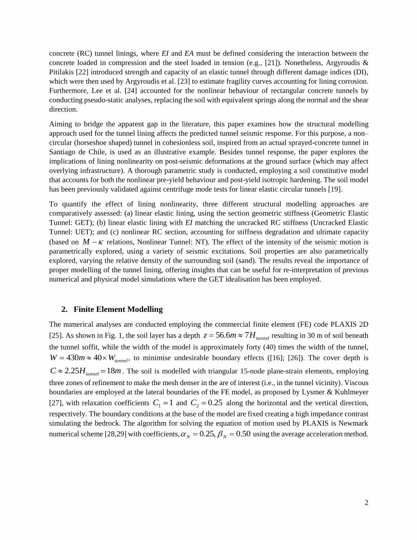
[25]. As shown in Fig. 1, the soil layer has a depth tunnelHmz 76.56 resulting in 30 m of soil beneath

the tunnel soffit, while the width of the model is approximately forty (40) times the width of the tunnel,

tunnelWmW 40430 , to minimise undesirable boundary effects ([16]; [26]). The cover depth is

mHC tunnel 1825.2 . The soil is modelled with triangular 15-node plane-strain elements, employing

three zones of refinement to make the mesh denser in the are of interest (i.e., in the tunnel vicinity). Viscous

boundaries are employed at the lateral boundaries of the FE model, as proposed by Lysmer & Kuhlmeyer

[27], with relaxation coefficients 11 C and 25.02 C along the horizontal and the vertical direction,

respectively. The boundary conditions at the base of the model are fixed creating a high impedance contrast

simulating the bedrock. The algorithm for solving the equation of motion used by PLAXIS is Newmark

numerical scheme [28,29] with coefficients, 50.0,25.0 NN using the average acceleration method.

3

Figure 1. FE model of the horseshoe tunnel, inspired from sprayed-concrete tunnels in Chile.

Since several previous studies have highlighted the importance of damping on the seismic response of

tunnels ([13]; [30]; [31]), two dissipation mechanisms are considered herein: (a) hysteretic damping, due

to nonlinear soil response (described later on); and (b) small additional frequency-dependent Rayleigh

damping:

ik

i

m fcf

c

4

1 (1)

where: is the additional equivalent viscous damping ratio, and if are characteristic frequencies related

to the model. The Rayleigh coefficients are set to 0005.0mc and 005.0kc , based on systematic

centrifuge testing of the soil underpinning the model parameter calibrations used herein ([32]; [33]). These

parameters result to a largely stiffness-proportional additional damping scheme, that filters high frequency

noise without overdamping lower frequencies, where most of the seismic energy is present.

The analyses are conducted in two steps. In the first step, the lining is defined assuming that it is constructed

under ideal conditions and thus no volume loss is considered as part of the analysis, and a geostatic analysis

is conducted. Based on the results of additional parametric analyses, for small volume loss values (less than

1%), the response of the tunnel is insensitive to the volume loss, especially for strong ground motions.

Therefore, the assumption of zero volume loss constitutes an acceptable limitation of the present study, and

the results presented herein can be considered realistic for modern tunnels that experience volume loss of

the order of 1% or lower ([34]; [35]). In the second step, the FE model is subjected to nonlinear dynamic

time history analysis.

2.1. Tunnel section

The horseshoe RC tunnel cross-section is shown in Fig. 2. This is a typical geometry for a sprayed-concrete

tunnel, inspired by Metro tunnels in Santiago de Chile, where the upper part (arch section) is circular with

constant radius mR 35.5 , intersecting at the bottom with a straight beam (flat section). At the joint of the

arch with the flat section, there lining is thicker with additional reinforcement, typically known as

“elephant’s foot” (due to its shape). Cross-sections A-A’ and B-B’ show the dimensions and reinforcement

in the arch and flat sections, respectively. The longitudinal reinforcement ranges from 8mm (D8) to 28mm

(D28). Qualitative moment-curvature ( M ) diagrams corresponding to each section are also shown the

4

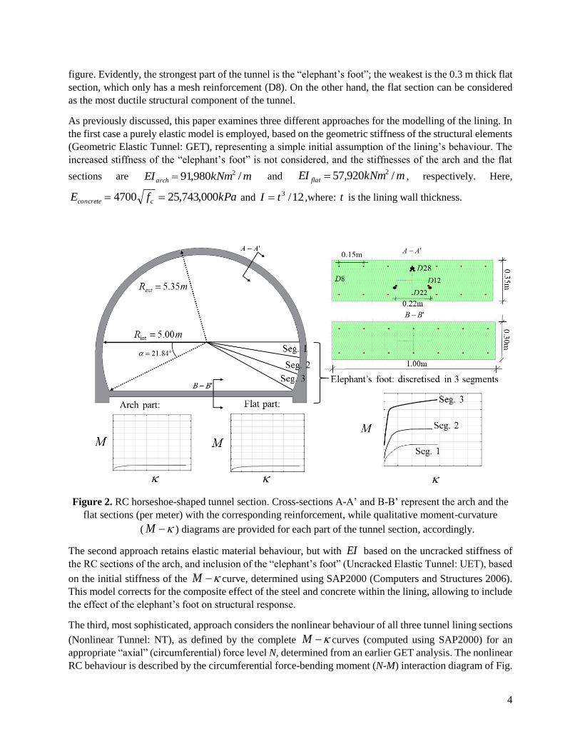
figure. Evidently, the strongest part of the tunnel is the “elephant’s foot”; the weakest is the 0.3 m thick flat

section, which only has a mesh reinforcement (D8). On the other hand, the flat section can be considered

as the most ductile structural component of the tunnel.

As previously discussed, this paper examines three different approaches for the modelling of the lining. In

the first case a purely elastic model is employed, based on the geometric stiffness of the structural elements

(Geometric Elastic Tunnel: GET), representing a simple initial assumption of the lining’s behaviour. The

increased stiffness of the “elephant’s foot” is not considered, and the stiffnesses of the arch and the flat

sections are mkNmEIarch /980,91 2 and mkNmEI flat /920,57 2 , respectively. Here,

kPafE cconcrete 000,743,254700 and 12/3tI ,where: t is the lining wall thickness.

Figure 2. RC horseshoe-shaped tunnel section. Cross-sections A-A’ and B-B’ represent the arch and the

flat sections (per meter) with the corresponding reinforcement, while qualitative moment-curvature

( M ) diagrams are provided for each part of the tunnel section, accordingly.

The second approach retains elastic material behaviour, but with EI based on the uncracked stiffness of

the RC sections of the arch, and inclusion of the “elephant’s foot” (Uncracked Elastic Tunnel: UET), based

on the initial stiffness of the M curve, determined using SAP2000 (Computers and Structures 2006).

This model corrects for the composite effect of the steel and concrete within the lining, allowing to include

the effect of the elephant’s foot on structural response.

The third, most sophisticated, approach considers the nonlinear behaviour of all three tunnel lining sections

(Nonlinear Tunnel: NT), as defined by the complete M curves (computed using SAP2000) for an

appropriate “axial” (circumferential) force level N, determined from an earlier GET analysis. The nonlinear

RC behaviour is described by the circumferential force-bending moment (N-M) interaction diagram of Fig.

5

3a, for both the arch and the flat sections. The points (circles) along the interaction curves signify the

moment capacities of the NT corresponding to the mean peak circumferential forces induced by Takarazuka

(TK) based ground motions (described in the next section) in the GET case. Fig. 3b shows the resulting

moment-curvature diagrams input to the NT models that correspond to section A-A’ in Fig. 2 and to

segments 1-3 of the “elephant’s foot” region for the case of MNN gTKGET 4.169.0, (TK-0.69g excitation).

Additionally, the corresponding UET (initial tangent stiffness of the M curves) and GET stiffnesses

are illustrated. For the UET and NT cases the “elephant’s foot” region is discretised into three distinct

segments to model the transition of the sectional properties within this region.

(a) (b)

Figure 3. (a) Axial force-bending moment interaction diagram for the arch and the flat section,

respectively, with corresponding points from the GET when subjected to the TK-based motions;

(b) Moment-curvature ( M ) curves of the arch section (A-A’), and of segments 1-3 of the elephant’s

foot region (NT model) along with M relations of the corresponding UET and GET models related to

the TK-0.69g ground motion.

Furthermore, a major parameter that can affect the seismic behaviour of tunnels is the interface between

the tunnel and the surrounding soil. In this study, given that the tunnels are formed from concrete sprayed

onto excavated soil, it is assumed that the interface between the shotcrete and the surrounding soil is fully

rough and thus the interface is considered as rigid (no slip condition).

2.2. Soil profile and constitutive modelling

The selected soil profile is based upon the stratigraphy of a real metro tunnel in Santiago, Chile. The soil

layer is modelled with a nonlinear elasto-plastic constitutive model with isotropic hardening after yielding

[36] coupled with a non-associative Mohr-Coulomb yield criterion [37] which is referred to as “hardening

soil model with small-strain stiffness” (HS small model) [38] in PLAXIS 2D. This constitutive model has

been previously validated against centrifuge tests of linear elastic tunnel models in clean sands [19]. The

ability of this model to produce representative site effect (ground motion amplification) in the free-field has

previously been demonstrated against centrifuge tests in [33], for ground motions of different strengths

inducing different amounts of inelastic soil response. However, the “HS small strain” soil model has

6

limitations in fully describing the dynamic behaviour of clean course-grained soils as it is not able to capture

reliably softening effects.

The pre-yield part of the model is represented by a nonlinear relation between the shear modulus, G , and

the shear strain, s , proposed by [39] and later modified by [40]:

7.0,

0385.01

1

s

sG

G

(2)

where: 0G is the small-strain shear modulus; and 7.0,s is the shear strain at 722.0/ 0 GG .

The paper utilises existing soil parameter calibrations for coarse-grained soil materials(see [32; [41]; [42])

with relative densities %100%,60rD , representative of medium dense and very dense sand, with similar

stiffness and strength to those reported for the alluvial material encountered in Santiago de Chile. These are

summarised in Table 1. These parameter calibrations have previously been shown to be applicable to

various granular materials [33] and have been validated against dynamic behaviour observed in centrifuge

experiments [32]. In addition to the nonlinear sG relationship defined by Eq. (2), the model also

accounts for the variation of 0G (and ) with confining stress (i.e., depth, z ):

m

ref

ref pc

c

G

G

'sin'cos'

'sin'cos' '

3

0

0

(3)

Figure 4. Distribution of shear wave velocity with depth for the soils considered in this study.

G

7

where: refG0 is the shear modulus at a reference stress, kPapref 100 ; c ’ is the effective cohesion; ' is

the effective friction angle; '

3 is the effective confining stress; and m is an empirical parameter controlling

the shape of the relationship. Figure 4 presents the distribution with depth of the shear wave velocity,

SV , resulting from:

0G

Vs (4)

The shear wave velocity profile of the soil is characterised as Ground type C ( smsmvs /180/28030,

) after EC8.

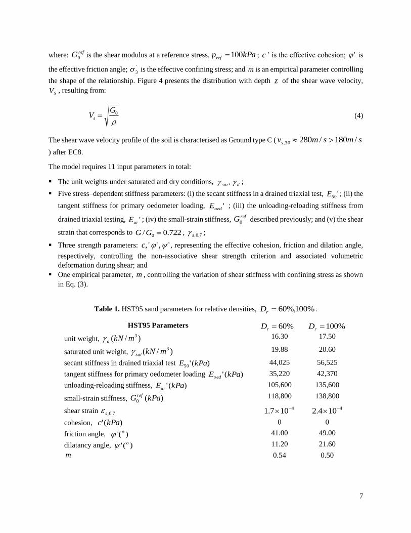
The model requires 11 input parameters in total:

The unit weights under saturated and dry conditions,dsat , ;

Five stress–dependent stiffness parameters: (i) the secant stiffness in a drained triaxial test, '50E ; (ii) the

tangent stiffness for primary oedometer loading, 'oedE ; (iii) the unloading-reloading stiffness from

drained triaxial testing, 'urE ; (iv) the small-strain stiffness, refG0 described previously; and (v) the shear

strain that corresponds to 722.0/ 0 GG , 7.0,s ;

Three strength parameters: ','', c , representing the effective cohesion, friction and dilation angle,

respectively, controlling the non-associative shear strength criterion and associated volumetric

deformation during shear; and

One empirical parameter, m , controlling the variation of shear stiffness with confining stress as shown

in Eq. (3).

Table 1. HST95 sand parameters for relative densities, %100%,60rD .

HST95 Parameters %60rD %100rD

unit weight, )/( 3mkNd 16.30 17.50

saturated unit weight, )/( 3mkNsat 19.88 20.60

secant stiffness in drained triaxial test )('50 kPaE 44,025 56,525

tangent stiffness for primary oedometer loading )(' kPaEoed 35,220 42,370

unloading-reloading stiffness, )(' kPaEur 105,600 135,600

small-strain stiffness, )(0 kPaG ref 118,800 138,800

shear strain 7.0,s 4107.1 4104.2

cohesion, )(' kPac 0 0

friction angle, )(' o 41.00 49.00

dilatancy angle, )(' o 11.20 21.60

m 0.54 0.50

z

8

The case considered in this paper considers the soil to be normally consolidated, such that the initial value

of the coefficient of earth pressure at rest is given by sin10K .

2.3. Ground motions

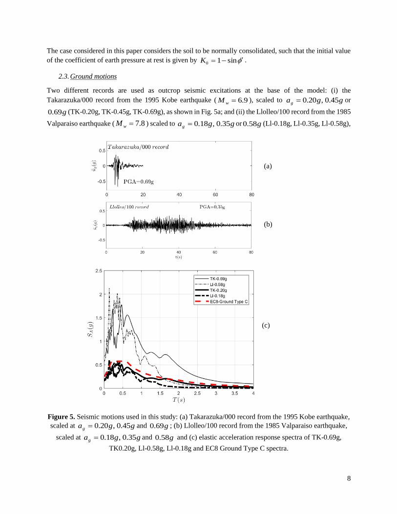
Two different records are used as outcrop seismic excitations at the base of the model: (i) the

Takarazuka/000 record from the 1995 Kobe earthquake ( 9.6wM ), scaled to ggag 45.0,20.0 or

g69.0 (TK-0.20g, TK-0.45g, TK-0.69g), as shown in Fig. 5a; and (ii) the Llolleo/100 record from the 1985

Valparaiso earthquake ( 8.7wM ) scaled to ggag 35.0,18.0 or g58.0 (Ll-0.18g, Ll-0.35g, Ll-0.58g),

Figure 5. Seismic motions used in this study: (a) Takarazuka/000 record from the 1995 Kobe earthquake,

scaled at ggag 45.0,20.0 and g69.0 ; (b) Llolleo/100 record from the 1985 Valparaiso earthquake,

scaled at ggag 35.0,18.0 and g58.0 and (c) elastic acceleration response spectra of TK-0.69g,

TK0.20g, Ll-0.58g, Ll-0.18g and EC8 Ground Type C spectra.

(a)

(b)

(c)

9

as shown in Fig. 5b. The specific two records were selected for two different reasons. The first is considered

representative of a severe seismic scenario, capable of inflicting significant damage to underground

structures, as was the case of the 1995 Kobe earthquale. The second is considered representative for Chile,

as it was recorded during the 1985 Valparaiso earthquake, one of the biggest recent earthquakes that struck

Chile. In addition, the TK-based motions are more intense time histories with coherent, predominant pulses

[43] while the Ll-based records are more far–field, long duration time histories without any distinguishable

predominant pulses.

Fig. 5c illustrates the response spectra of the scaled TK-based and Ll-based records, for the smallest and

largest motions, also showing the design spectra suggested by Eurocode 8 [44] for ground type C for

context. In Fig.5c nominal structural damping of %5 is assumed.

3. The effect of lining model on tunnel response

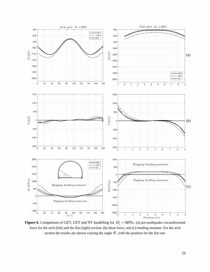
Figure 6 presents the envelopes of the residual pre-earthquake lining forces as a result of the first phase:

geostatic analysis. The bending moment plot convention follows the deformed shape of the lining, thus

negative moment signifies tension on the bottom side of the structural elements. The term “sagging” is used

to refer to negative moments of the arch section and the positive moments of the flat section (i.e.,

representing bending inwards into the tunnel void). The term “hogging” is used to refer to the positive

bending moments of the arch section and the negative of the flat section.

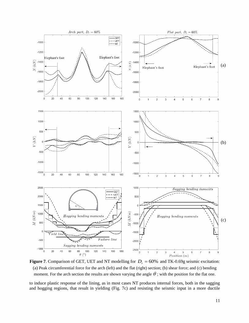
Additionally, Figure 7 shows the envelopes of the lining forces for the GET, UET and NT cases, using TK-

0.69g as seismic excitation. In Fig. 7c, the thick black continuous lines represent the final points of the

M curves defined as failure lines, while, the thick continuous gray lines represent the yield points of

the M curves, defined as yield lines. The yield point is defined as the first yield of any rebar of the

sections shown in Fig. 2 [45]. The three forming “steps” of the yield and failure lines correspond to the

three different segments at the “elephant’s foot” region for the arch section (as shown in Fig. 2), as is the

single step of the yielding and failure lines in the case of the flat section.

A first observation from Fig. 7 is that the arch section develops higher circumferential forces than the flat

section, while the exact opposite is observed for the shear forces where the flat section resembles a typical

beam. This behavior is a result of the different structural forms and more specifically, the arch section tends

to propagate compressive loads as circumferential forces while the flat section tends to bend producing

higher shear forces. Figure 7c illustrates the maximum bending moments developed in the tunnel. While

no yielding is observed close to the tunnel crown, this is not the case for the section close to the “elephant’s

foot”. However, in the case of the flat section, there is yielding all along its length, which is close to failure.

This is an important result that practicing engineers need to consider in the preliminary design, but also in

the detailing of the reinforcement with regards to horseshoe-type tunnel sections.

Regarding the elastic structural models, GET and UET, it is evident from Fig. 7 that UET gives more

conservative results as it represents a stiffer configuration (as shown in Fig. 3). Furthermore, GET

underestimates the internal forces, particularly the bending moments, at the “elephant’s foot” region since

this area is not considered at all in this model. Therefore, it is important to account for changes in the

stiffness along the tunnel section, as the distribution of the internal forces depends highly on that – stiffer

regions attract larger loads and “relieve” accordingly other parts of the tunnel.

The comparison between the UET and NT models reveal interesting aspects of nonlinear structural

behavior, as a function of the seismic demand. It is clear that the ground motion is strong enough

10

Figure 6. Comparison of GET, UET and NT modelling for %60rD : (a) pre-earthquake circumferential

force for the arch (left) and the flat (right) section; (b) shear force; and (c) bending moment. For the arch

section the results are shown varying the angle ; with the position for the flat one.

(a)

(b)

(c)

11

Figure 7. Comparison of GET, UET and NT modelling for %60rD and TK-0.69g seismic excitation:

(a) Peak circumferential force for the arch (left) and the flat (right) section; (b) shear force; and (c) bending

moment. For the arch section the results are shown varying the angle ; with the position for the flat one.

to induce plastic response of the lining, as in most cases NT produces internal forces, both in the sagging

and hogging regions, that result in yielding (Fig. 7c) and resisting the seismic input in a more ductile

(a)

(b)

(c)

12

fashion. Hence, the consideration of the uncracked elastic RC section (UET) may lead to larger lining

sections and more reinforcement demands, since the ductility of the tunnel section is not accounted for.

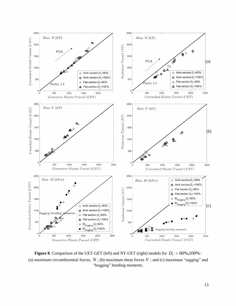
Figure 8 presents a comparison between the peak lining forces for the GET, UET and NT models for relative

soil densities, %100%,60rD . From Figs. 7a and 7b, it can be deduced that the UET model develops

higher peak lining forces in almost all cases examined, since it represents the stiffest configuration (see also

Fig. 7). The only exception is the “sagging” bending moments of the flat section, where the GET predicts

higher values; this is due to the consideration of the “elephant’s foot” region in the UET model assuming

stiffer support of the flat section (higher “hogging” moments) and thus relieving the midspan (“sagging”

moments) accordingly.

Figures 8a, 8b and 8c show that the NT model develops much lower values of peak lining forces, as

expected, due to its more ductile behaviour and to the pre-defined capacity from the M curves. The

differences between the two models also reveal the effect of the nonlinear behaviour of lining structural

elements on the seismic performance of the tunnel. Focusing more on the NT model, from Figs. 8b and 8c,

it is shown that the lower relative density, %60rD , results in larger circumferential forces than for the

very dense case, %100rD . The same is true for the shear forces of the arch section, but the exact

opposite is observed for the shear forces of the flat section, showing that the denser sand tends to dilate

more towards the ground surface inducing higher stresses on the flat section by bending upwards.

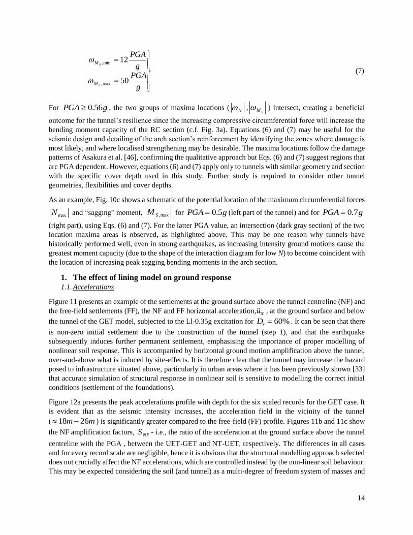
Figure 9 focuses on the peak “sagging” and “hogging” moments for the arch and the flat parts, respectively.

Fig. 9a shows that the arch section does not yield for any seismic excitation (circular markers do not cross

the yielding/dashed or failure/dotted lines, respectively), while the flat section yields and enters the plastic

region extensively along its length and is close to failure for almost all ground motions and for both relative

densities (circular markers above the yielding/dashed line and very close to the failure/dotted line). This is

not unexpected given that the moment capacity of the flat section is substantially lower than that of the arch

(Figure 3a). Conversely, Fig. 9c shows that the “hogging” moments remain in the elastic region, far from

yielding; the values for the arch and the flat sections coincide as the maxima are located near the intersection

(or the “elephant’s foot” region/supports of the flat section). From Figs. 7a and 7c it is evident that the

location of the peak compressive circumferential forces and the “sagging” moments of the arch section are

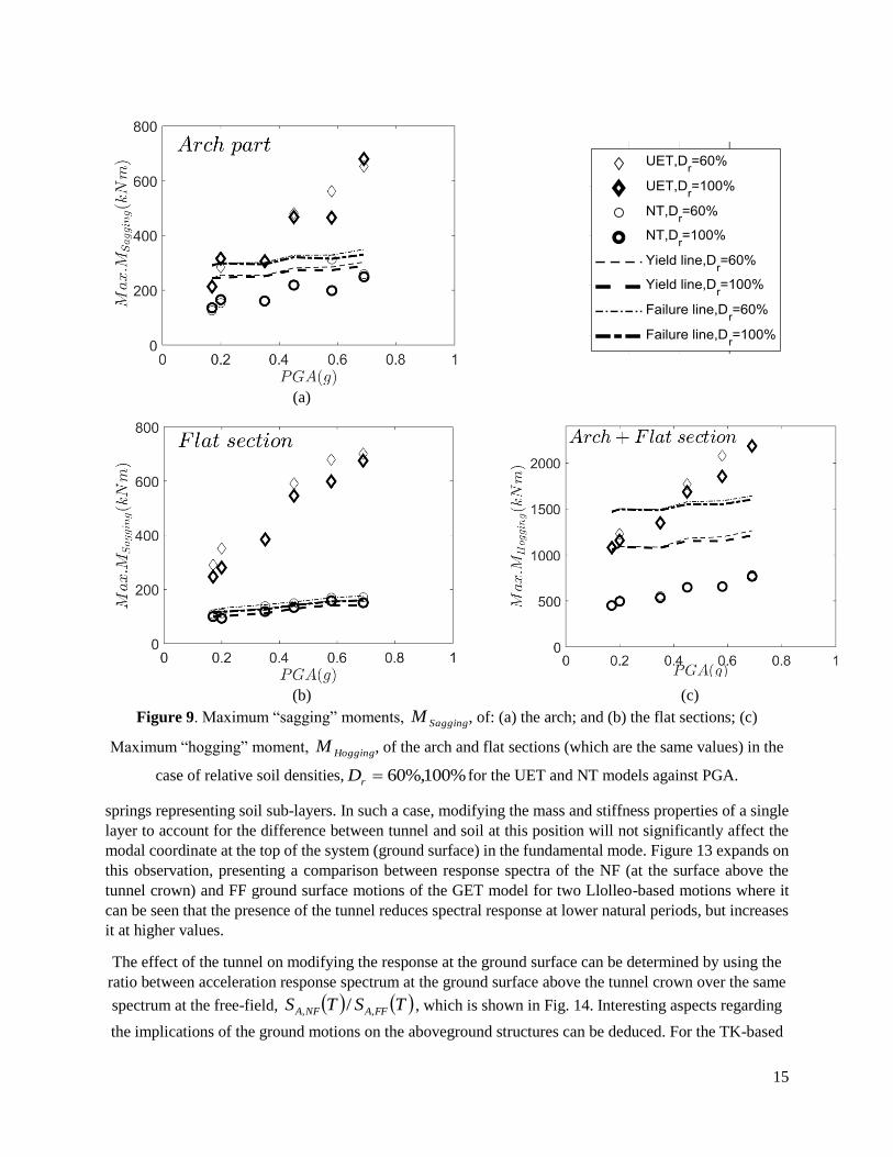
not located at the tunnel crown, but rather at an angle, , away from the tunnel centreline. If it is assumed

that the tunnel centreline is at o0 , Fig. 10 presents the offset angle from the tunnel crown where the

maximum compressive circumferential forces (Fig. 10a) N occur and where the maximum “sagging”

moments (Fig. 10b) SM occur, for all structural models (GET, UET, NT). Figure 10a shows that as the

seismic intensity increases (PGA) the point where the circumferential forces are maximized tends to move

closer to the tunnel centreline and the bounds of these location points are given by:

g

PGA

g

PGA

N

N

3070

3045

max,

min,

(6)

Figure 10b shows that as the PGA increases the location of the maximum “sagging” moments moves away

from the tunnel’s centreline with upper and lower bounds of:

13

Figure 8. Comparison of the UET-GET (left) and NT-UET (right) models for %100%,60rD :

(a) maximum circumferential forces, N ; (b) maximum shear forces V ; and (c) maximum “sagging” and

“hogging” bending moments.

(a)

(c)

(b)

14

g

PGA

g

PGA

S

S

M

M

50

12

max,

min,

(7)

For gPGA 56.0 , the two groups of maxima locations ( N ,SM ) intersect, creating a beneficial

outcome for the tunnel’s resilience since the increasing compressive circumferential force will increase the

bending moment capacity of the RC section (c.f. Fig. 3a). Equations (6) and (7) may be useful for the

seismic design and detailing of the arch section’s reinforcement by identifying the zones where damage is

most likely, and where localised strengthening may be desirable. The maxima locations follow the damage

patterns of Asakura et al. [46], confirming the qualitative approach but Eqs. (6) and (7) suggest regions that

are PGA dependent. However, equations (6) and (7) apply only to tunnels with similar geometry and section

with the specific cover depth used in this study. Further study is required to consider other tunnel

geometries, flexibilities and cover depths.

As an example, Fig. 10c shows a schematic of the potential location of the maximum circumferential forces

maxN and “sagging” moment, max,SM for gPGA 5.0 (left part of the tunnel) and for gPGA 7.0

(right part), using Eqs. (6) and (7). For the latter PGA value, an intersection (dark gray section) of the two

location maxima areas is observed, as highlighted above. This may be one reason why tunnels have

historically performed well, even in strong earthquakes, as increasing intensity ground motions cause the

greatest moment capacity (due to the shape of the interaction diagram for low N) to become coincident with

the location of increasing peak sagging bending moments in the arch section.

1. The effect of lining model on ground response

1.1. Accelerations

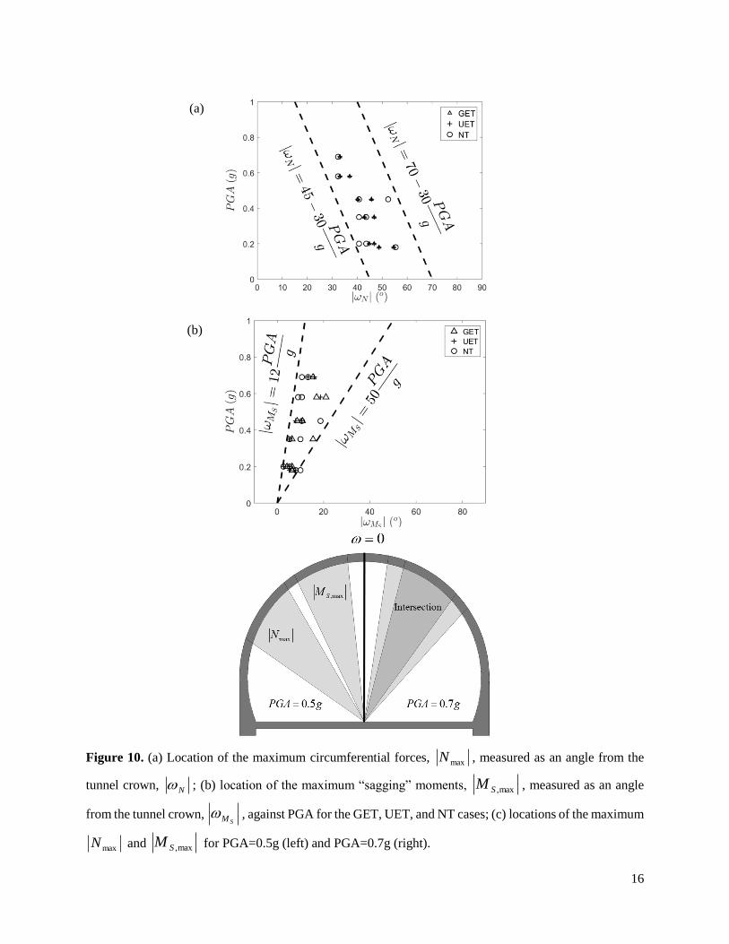
Figure 11 presents an example of the settlements at the ground surface above the tunnel centreline (NF) and

the free-field settlements (FF), the NF and FF horizontal acceleration,�̈�𝑥 , at the ground surface and below

the tunnel of the GET model, subjected to the Ll-0.35g excitation for %60rD . It can be seen that there

is non-zero initial settlement due to the construction of the tunnel (step 1), and that the earthquake

subsequently induces further permanent settlement, emphasising the importance of proper modelling of

nonlinear soil response. This is accompanied by horizontal ground motion amplification above the tunnel,

over-and-above what is induced by site-effects. It is therefore clear that the tunnel may increase the hazard

posed to infrastructure situated above, particularly in urban areas where it has been previously shown [33]

that accurate simulation of structural response in nonlinear soil is sensitive to modelling the correct initial

conditions (settlement of the foundations).

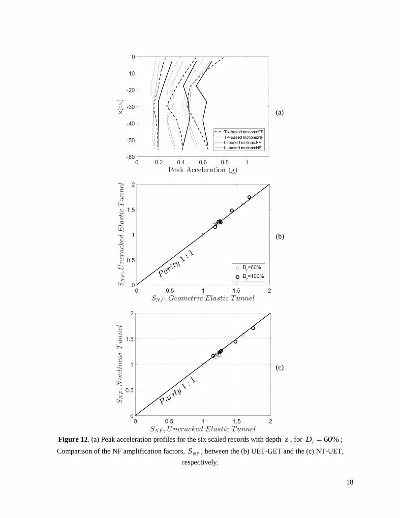
Figure 12a presents the peak accelerations profile with depth for the six scaled records for the GET case. It

is evident that as the seismic intensity increases, the acceleration field in the vicinity of the tunnel

( mm 2618 ) is significantly greater compared to the free-field (FF) profile. Figures 11b and 11c show

the NF amplification factors, NFS - i.e., the ratio of the acceleration at the ground surface above the tunnel

centreline with the PGA , between the UET-GET and NT-UET, respectively. The differences in all cases

and for every record scale are negligible, hence it is obvious that the structural modelling approach selected

does not crucially affect the NF accelerations, which are controlled instead by the non-linear soil behaviour.

This may be expected considering the soil (and tunnel) as a multi-degree of freedom system of masses and

15

(a)

(b) (c)

Figure 9. Maximum “sagging” moments, SaggingM , of: (a) the arch; and (b) the flat sections; (c)

Maximum “hogging” moment, HoggingM , of the arch and flat sections (which are the same values) in the

case of relative soil densities, %100%,60rD for the UET and NT models against PGA.

springs representing soil sub-layers. In such a case, modifying the mass and stiffness properties of a single

layer to account for the difference between tunnel and soil at this position will not significantly affect the

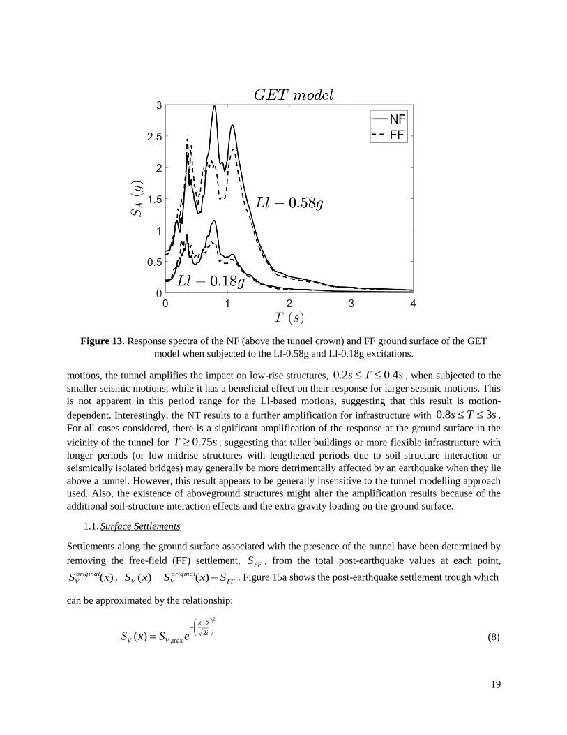
modal coordinate at the top of the system (ground surface) in the fundamental mode. Figure 13 expands on

this observation, presenting a comparison between response spectra of the NF (at the surface above the

tunnel crown) and FF ground surface motions of the GET model for two Llolleo-based motions where it

can be seen that the presence of the tunnel reduces spectral response at lower natural periods, but increases

it at higher values.

The effect of the tunnel on modifying the response at the ground surface can be determined by using the

ratio between acceleration response spectrum at the ground surface above the tunnel crown over the same

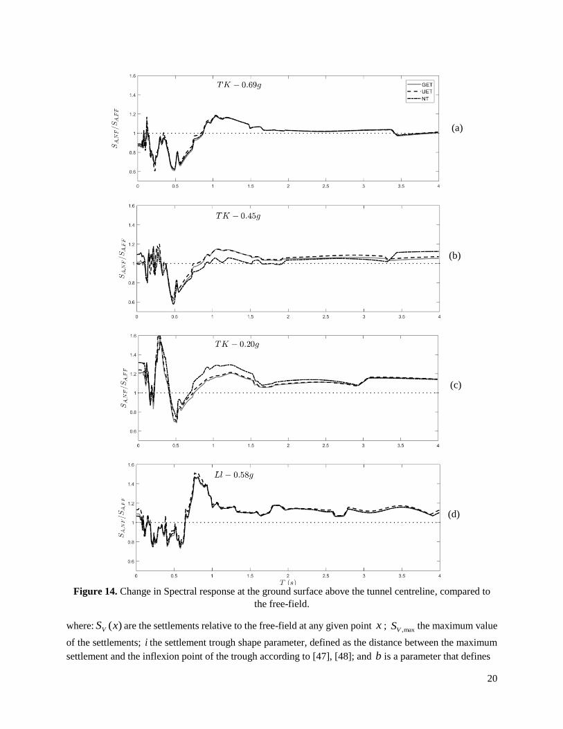
spectrum at the free-field, TSTS FFANFA ,, / , which is shown in Fig. 14. Interesting aspects regarding

the implications of the ground motions on the aboveground structures can be deduced. For the TK-based

16

Figure 10. (a) Location of the maximum circumferential forces, maxN , measured as an angle from the

tunnel crown, N ; (b) location of the maximum “sagging” moments, max,SM , measured as an angle

from the tunnel crown, SM , against PGA for the GET, UET, and NT cases; (c) locations of the maximum

maxN and max,SM for PGA=0.5g (left) and PGA=0.7g (right).

(a)

(b)

17

Figure 11. (a) NF (above the tunnel centreline) and FF settlements at the ground surface; (b) NF and FF

horizontal acceleration, �̈�𝑥, at the ground surface above the tunnel centreline; (c) NF and FF horizontal

acceleration, �̈�𝑥, below the tunnel when the soil profile is excited by (d) Ll-0.35g excitation

(a)

(b)

(c)

(d)

18

Figure 12. (a) Peak acceleration profiles for the six scaled records with depth z , for %60rD ;

Comparison of the NF amplification factors, NFS , between the (b) UET-GET and the (c) NT-UET,

respectively.

(a)

(b)

(c)

19

Figure 13. Response spectra of the NF (above the tunnel crown) and FF ground surface of the GET

model when subjected to the Ll-0.58g and Ll-0.18g excitations.

motions, the tunnel amplifies the impact on low-rise structures, sTs 4.02.0 , when subjected to the

smaller seismic motions; while it has a beneficial effect on their response for larger seismic motions. This

is not apparent in this period range for the Ll-based motions, suggesting that this result is motion-

dependent. Interestingly, the NT results to a further amplification for infrastructure with sTs 38.0 .

For all cases considered, there is a significant amplification of the response at the ground surface in the

vicinity of the tunnel for sT 75.0 , suggesting that taller buildings or more flexible infrastructure with

longer periods (or low-midrise structures with lengthened periods due to soil-structure interaction or

seismically isolated bridges) may generally be more detrimentally affected by an earthquake when they lie

above a tunnel. However, this result appears to be generally insensitive to the tunnel modelling approach

used. Also, the existence of aboveground structures might alter the amplification results because of the

additional soil-structure interaction effects and the extra gravity loading on the ground surface.

1.1. Surface Settlements

Settlements along the ground surface associated with the presence of the tunnel have been determined by

removing the free-field (FF) settlement, FFS , from the total post-earthquake values at each point,

)(xS original

V,

FF

original

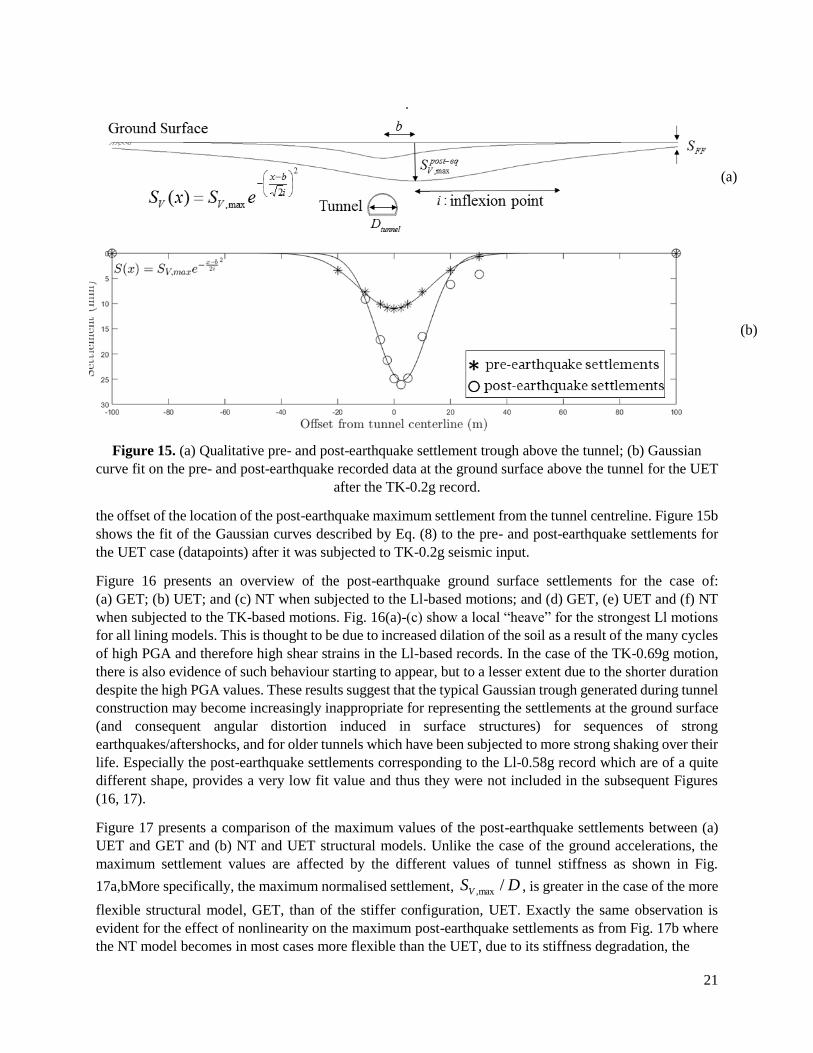
VV SxSxS )()( . Figure 15a shows the post-earthquake settlement trough which

can be approximated by the relationship:

2

2max,)(

i

bx

VV eSxS (8)

20

Figure 14. Change in Spectral response at the ground surface above the tunnel centreline, compared to

the free-field.

where: )(xSV are the settlements relative to the free-field at any given point x ; max,VS the maximum value

of the settlements; i the settlement trough shape parameter, defined as the distance between the maximum

settlement and the inflexion point of the trough according to [47], [48]; and b is a parameter that defines

(a)

(b)

(c)

(d)

21

.

Figure 15. (a) Qualitative pre- and post-earthquake settlement trough above the tunnel; (b) Gaussian

curve fit on the pre- and post-earthquake recorded data at the ground surface above the tunnel for the UET

after the TK-0.2g record.

the offset of the location of the post-earthquake maximum settlement from the tunnel centreline. Figure 15b

shows the fit of the Gaussian curves described by Eq. (8) to the pre- and post-earthquake settlements for

the UET case (datapoints) after it was subjected to TK-0.2g seismic input.

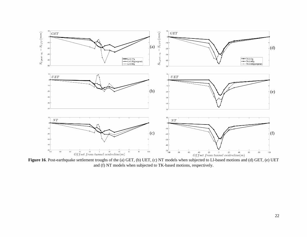
Figure 16 presents an overview of the post-earthquake ground surface settlements for the case of:

(a) GET; (b) UET; and (c) NT when subjected to the Ll-based motions; and (d) GET, (e) UET and (f) NT

when subjected to the TK-based motions. Fig. 16(a)-(c) show a local “heave” for the strongest Ll motions

for all lining models. This is thought to be due to increased dilation of the soil as a result of the many cycles

of high PGA and therefore high shear strains in the Ll-based records. In the case of the TK-0.69g motion,

there is also evidence of such behaviour starting to appear, but to a lesser extent due to the shorter duration

despite the high PGA values. These results suggest that the typical Gaussian trough generated during tunnel

construction may become increasingly inappropriate for representing the settlements at the ground surface

(and consequent angular distortion induced in surface structures) for sequences of strong

earthquakes/aftershocks, and for older tunnels which have been subjected to more strong shaking over their

life. Especially the post-earthquake settlements corresponding to the Ll-0.58g record which are of a quite

different shape, provides a very low fit value and thus they were not included in the subsequent Figures

(16, 17).

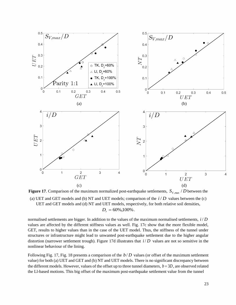
Figure 17 presents a comparison of the maximum values of the post-earthquake settlements between (a)

UET and GET and (b) NT and UET structural models. Unlike the case of the ground accelerations, the

maximum settlement values are affected by the different values of tunnel stiffness as shown in Fig.

17a,bMore specifically, the maximum normalised settlement, DSV /max, , is greater in the case of the more

flexible structural model, GET, than of the stiffer configuration, UET. Exactly the same observation is

evident for the effect of nonlinearity on the maximum post-earthquake settlements as from Fig. 17b where

the NT model becomes in most cases more flexible than the UET, due to its stiffness degradation, the

(a)

(b)

22

Figure 16. Post-earthquake settlement troughs of the (a) GET, (b) UET, (c) NT models when subjected to Ll-based motions and (d) GET, (e) UET

and (f) NT models when subjected to TK-based motions, respectively.

(a) (d)

(e)

(f)

(b)

(c)

23

(a) (b)

(c) (d)

Figure 17. Comparison of the maximum normalized post-earthquake settlements, DSV /max, between the

(a) UET and GET models and (b) NT and UET models; comparison of the Di / values between the (c)

UET and GET models and (d) NT and UET models, respectively, for both relative soil densities,

%100%,60rD .

normalised settlements are bigger. In addition to the values of the maximum normalised settlements, Di /

values are affected by the different stiffness values as well. Fig. 17c show that the more flexible model,

GET, results to higher values than in the case of the UET model. Thus, the stiffness of the tunnel under

structures or infrastructure might lead to unwanted post-earthquake settlement due to the higher angular

distortion (narrower settlement trough). Figure 17d illustrates that Di / values are not so sensitive in the

nonlinear behaviour of the lining.

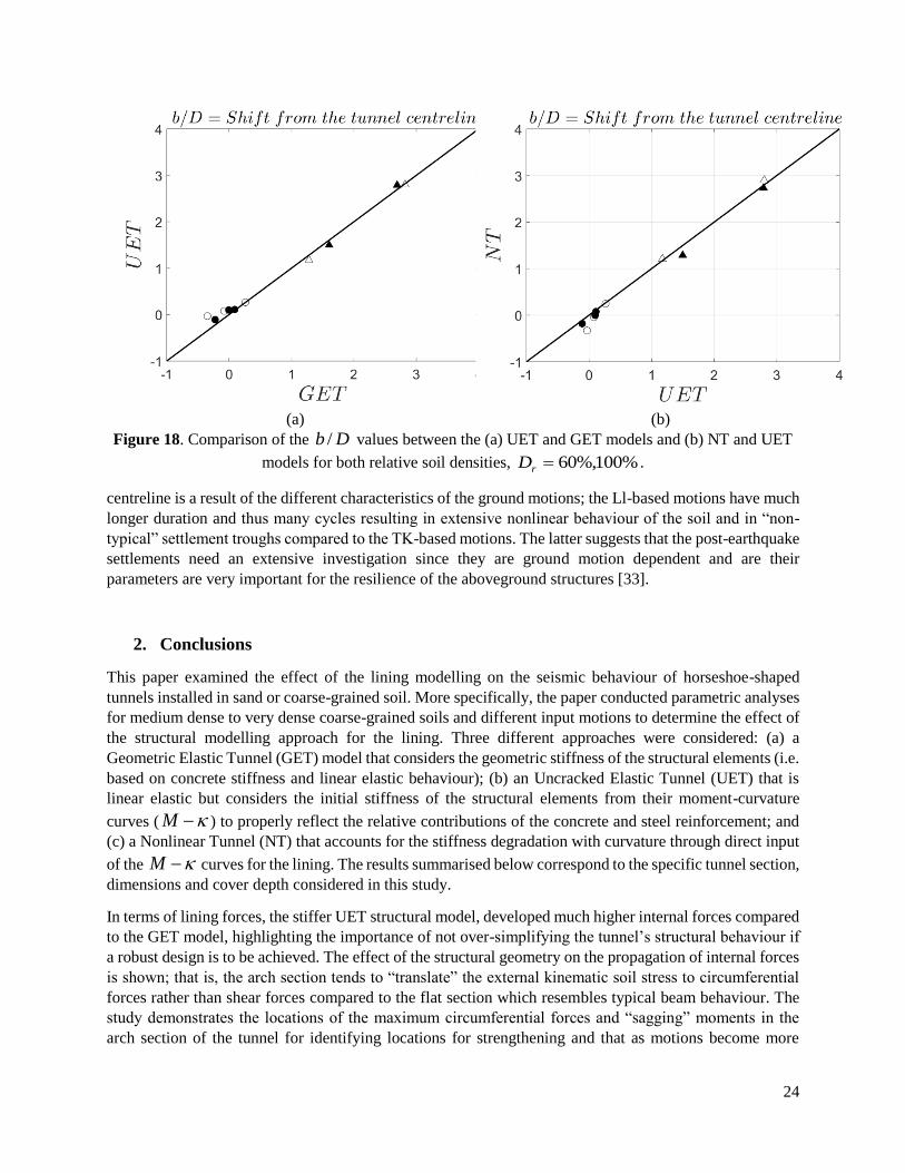
Following Fig. 17, Fig. 18 presents a comparison of the Db / values (or offset of the maximum settlement

value) for both (a) UET and GET and (b) NT and UET models. There is no significant discrepancy between

the different models. However, values of the offset up to three tunnel diameters, Db 3 , are observed related

the Ll-based motions. This big offset of the maximum post-earthquake settlement value from the tunnel

(a)

24

(a) (b)

Figure 18. Comparison of the Db / values between the (a) UET and GET models and (b) NT and UET

models for both relative soil densities, %100%,60rD .

centreline is a result of the different characteristics of the ground motions; the Ll-based motions have much

longer duration and thus many cycles resulting in extensive nonlinear behaviour of the soil and in “non-

typical” settlement troughs compared to the TK-based motions. The latter suggests that the post-earthquake

settlements need an extensive investigation since they are ground motion dependent and are their

parameters are very important for the resilience of the aboveground structures [33].

2. Conclusions

This paper examined the effect of the lining modelling on the seismic behaviour of horseshoe-shaped

tunnels installed in sand or coarse-grained soil. More specifically, the paper conducted parametric analyses

for medium dense to very dense coarse-grained soils and different input motions to determine the effect of

the structural modelling approach for the lining. Three different approaches were considered: (a) a

Geometric Elastic Tunnel (GET) model that considers the geometric stiffness of the structural elements (i.e.

based on concrete stiffness and linear elastic behaviour); (b) an Uncracked Elastic Tunnel (UET) that is

linear elastic but considers the initial stiffness of the structural elements from their moment-curvature

curves ( M ) to properly reflect the relative contributions of the concrete and steel reinforcement; and

(c) a Nonlinear Tunnel (NT) that accounts for the stiffness degradation with curvature through direct input

of the M curves for the lining. The results summarised below correspond to the specific tunnel section,

dimensions and cover depth considered in this study.

In terms of lining forces, the stiffer UET structural model, developed much higher internal forces compared

to the GET model, highlighting the importance of not over-simplifying the tunnel’s structural behaviour if

a robust design is to be achieved. The effect of the structural geometry on the propagation of internal forces

is shown; that is, the arch section tends to “translate” the external kinematic soil stress to circumferential

forces rather than shear forces compared to the flat section which resembles typical beam behaviour. The

study demonstrates the locations of the maximum circumferential forces and “sagging” moments in the

arch section of the tunnel for identifying locations for strengthening and that as motions become more

25

intense, an RC tunnel reinforces itself as the location of maximum circumferential force becomes coincident

with the region of maximum bending moment. In the horseshoe shaped tunnels tested, the springing

locations are key design areas, as is the flat bottom of the tunnel (in the absence of any vehicle load or

stiffening from the track/roadway). Furthermore, medium-dense coarse-grained soils lead to higher lining

forces in most cases with the exception of the flat bottom of the tunnel where the denser soil dilates towards

the ground surface and bends it accordingly.

The modelling approach selected does not appear to affect the acceleration field at the ground surface above

the tunnel significantly, though it does have a more significant effect on ground settlement (both gross and

relative to the free-field), with non-linear behaviour resulting in larger and more rapidly changing

settlements, which could be damaging to surface buildings and infrastructures in the vicinity of the tunnel.

In all cases spectral response at low natural periods ( sTs 4.02.0 i.e. low-rise structures) was motion

sensitive, while for higher periods ( sT 8.0 ) the presence of the tunnel generally increased seismic

response between 20-50% (motion sensitive). It was shown that with extended extensive high PGA shaking,

the typical Gaussian settlement trough which is deepened by lower intensity shaking, changes shape

dramatically in these dilative soils.

Acknowledgements

This work was supported by the Newton Fund: EPSRC, UK & CONICYT Chile: Shaking tunnel vision.

Joint project led by University of Leeds EP/N03435X/1.

References

[1] Dowding CH, Rozen A. Damage to rock tunnels from earthquake shaking. Journal of Geotechnical

Engineering Division 1978; 104(GT2): 175–191.

[2] Wang JN. Seismic design of tunnels: A state-of-the-art approach. Monograph 7. New York: Parsons,

Brinckerhoff, Quade and Douglas, Inc; 1993.

[3] Kawashima, K. Seismic design of underground structures in soft ground, a review. Proceedings of the

International Symposium on Tunneling in Difficult Ground Conditions. Tokyo, Japan; 1999.

[4] Anastasopoulos I, Gazetas G. Analysis of cut-and-cover tunnels against large tectonic deformation.

Bulletin of Earthquake Engineering 2010; 35: 1-12.

[5] Tsinidis G, Pitilakis K and Anagnostopoulos C. Circular tunnels in sand: dynamic response and

efficiency of seismic analysis methods at extreme lining flexibilities. Bulletin of Earthquake

Engineering 2016a; 14: 2903–29.

[6] Tsinidis G, Pitilakis K and Madabhushi G. On the dynamic response of square tunnels in sand.

Engineering Structures 2016b; 125: 419–437.

[7] Iida H, Hiroto T, Yoshida N, Iwafuji M. Damage to Daikai subway station. Special issue on

geotechnical aspects of the January 17 1995 Hyogoken–Nanbu earthquake. Soils Foundations 1996;

283–300.

[8] Nakamura S, Yoshida N, Iwatate T. Damage to Daikai subway station during the 1995 Hyogoken–

Nambu earthquake and its investigation 1996; 287–295.

[9] Ueng TS, Lin ML, and Chen MH. Some geotechnical aspects of 1999 Chi-Chi, Taiwan earthquake.

Proceedings of the Fourth International Conference on Recent Advances in Geotechnical Earthquake

Engineering and Soil Dynamics SPL-10.1, 5 p.1-5; 2001.

26

[10] O’ Rourke TD, Goh SH, Menkiti CO and Mair RJ. Highway tunnel performance during the 1999

Düzce earthquake. In: Proceedings of the 15th International Conference on Soil Mechanics and

Geotechnical Engineering, August 27–31, Istanbul; 2001.

[11] Yoshida N. Damage to subway station during the 1995 Hyogoken-Nambu (Kobe) earthquake. In T.

Kokusho (Ed.), Earthquake geotechnical case histories for performance-based design. Tokyo: CRC

Press, pp. 373–389; 2009.

[12] Hashash YMA, Hook JJ, Schmidt B, Yao JI-C. Seismic design and analysis of underground structures.

Tunnel and Underground Space Technologies 2001; 16(2): 247–293.

[13] Kontoe S Zdravkovic L, Potts DM, Menkiti, CO. On the relative merits of simple and advanced

constitutive models in dynamic analysis of tunnels. Geotechnique 2011; 61(10): 815-829.

[14] Anastasopulos I, Gerolymos N, Drosos V, Kourkoulis R, Georgakakos T, Gazetas G. Nonlinear

response of deep immersed tunnel to strong seismic shaking. Journal of Geotechnical and

Feoenvironmental Engineering 2007; 133(9): 1067-1090.

[15] Anastasopulos I, Gerolymos N, Drosos V, Georgakakos T, Kourkoulis R, Gazetas G. Nonlinear

response of deep immersed tunnel to strong seismic shaking. Bulletin of Earthquake Engineering 2008;

6: 213-239.

[16] Amorosi A, Boldini D. Numerical modelling of the transverse dynamic behaviour of circular tunnels

in clayey soils. Soil Dynamic and Earthquake Engineering 2009; 29(6): 1059–72.

[17] Cilingir U, Madabhushi SPG. Effect of depth on the seismic response of circular tunnels. Canadian

Geotechnical Journal 2011a; 48(1): 117–27.

[18] Cilingir U, Madabhushi SPG. A model study on the effects of input motion on the seismic behaviour

of tunnels. Soil Dynamics and Earthquake Engineering 2011b; 31: 452–62.

[19] Bilotta E, Lanzano G, Madabhushi SPG, Silvestri, F. A numerical Round Robin on tunnels under

seismic actions. Acta Geotechnica 2014; 9: 563-579.

[20] Tsinidis G, Pitilakis K, Madabhushi G and Heron C. Dynamic response of flexible square tunnels:

centrifuge testing and validation of existing design methodologies. Geotechnique 2015; 65(5): 401–

417.

[21] Knappett JA. Discussion on paper “Design charts for seismic analysis of single piles in clay” by A.

Tabesh and H.G. Poulos. Proc. ICE, Geotechnical Engng, 161(GE2): 115-116. DOI:

10.1680/geng.2008.161.2.115; 2008. [22] Argyroudis S., Pitilakis, K. Seismic fragility curves of shallow tunnels in alluvial deposits. Soil

Dynamics and Earthquake Engineering 2012; 98: 244-256.

[23] Argyroudis S, Tsinidis G, Gatti F, Pitilakis K. Effects of SSI and lining corrosion on the seismic

vulnerability of shallow circular tunnels. Soil Dynamics and Earthquake Engineering 2017; 98: 244-

256.

[24] Lee TH, Park D, Nguyen DD, Park JS. Damage analysis of cut-and-cover tunnel structures under

seismic loading. Bulletin of Earthquake Engineering 2016;14: 413-431.

[25] Brinkgreve RBJ and Vermeer PA. Plaxis manual. Version, 7, 5-1; 1998.

[26] Amorosi A, Boldini D, Gaetano E. Parametric study on seismic ground response by finite element

modelling. Computers and Geotechnics 2010; 37: 515-528.

[27] Lysmer J and Kuhlmeyer RL. Finite dynamic model for infinite media. Journal of Engineering

Mechanics Division, ASCE 1969; 95(4): 859–887.

[28] Newmark, N.M. "A Method of Computation for Structural Dynamics" ASCE Journal of Engineering

Mechanics Division, 1959; 85. No EM3.

[29] Chopra, A. K. Dynamics of structures: Theory and applications to earthquake engineering. Englewood

Cliffs, NJ: Prentice Hall, 2001.

[30] Zerwer A, Cascante G and Hutchinson J. Parameter estimation in finite element simulations of

Rayleigh waves. Journal of Geotechnical and Geoenvironmental Engineering 2002; 128(3): 250–261.

[31] Kwok AOL, Stewart JP, Hashash YMA, Matasovic N, Pyke R, Wang Z. Use of exact solutions of

wave propagation problems to guide implementation of nonlinear seismic ground response analysis

procedures. Journal of Geotechnical and Geoenvironmental Engineering 2007; 133(11): 1385–98.

27

[32] Al-Defae, AH, Caucis K, Knappett JA. Aftershocks and the whole-life seismic performance of

granular slopes. Géotechnique 2013; 63(14): 1230–1244.

[33] Knappett JA, Madden P, Caucis K. Seismic structure-soil-structure interaction between pairs of

adjacent building structures. Geotechnique 2015; 65(5): 429-441.

[34] High Speed Two Ltd. (2013). Impacts of Tunnels in the UK. Department of Transport, London.

[35] Coulter S and Martin DC (2004). Ground Deformations Above a Shallow Tunnel Excavated Using Jet

Grouting. Proc. ISRM Regional Symposium EUROCK 2004 and 53rd Geomechanics Colloquy, 155-

160, VGE, Essen.

[36] Schanz T, Vermeer PA, Bonnier PG. The hardening soil model: formulation and verification. In

Beyond 2000 in computation geotechnics (ed. RBJ Brinkgreve), pp. 281–290. Rotterdam, the

Netherlands: Balkema; 1999.

[37] Smith IM, Griffiths DV. Programming the Finite Element Method. John Wiley & Sons, Chisester,

U.K., 2nd edition; 1982.

[38] Benz T. Small-strain stiffness of soils and its numerical consequences. PhD thesis, University of

Stuttgart, Germany; 2006.

[39] Hardin BO, Drnevich VP. Shear modulus and damping in soils: design equations and curves. Journal

of Soil Mechanics Foundations Division ASCE 1972; 98(SM7): 667–692.

[40] Santos JA and Correia AG. Reference threshold shear strain of soil: its application to obtain a unique

strain-dependent shear modulus curve for soil. Proceedings of the 15th international conference on soil

mechanics and geotechnical engineering, Istanbul, Turkey, vol. 1, pp. 267–270; 2001.

[41] Lauder K, Brown MJ, Bransby MF and Boyes S. The influence of incorporating a forecutter on the

performance of offshore pipeline ploughs. Applied Ocean Research Journal 2013; 39: 121-130. DOI:

10.1016/j.apor.2012.11.001.

[42] Bransby MF, Brown MJ, Knappett JA, Hudacsek P, Morgan N, Cathie D, Maconochie A, Yun G,

Ripley AG, Brown N, Egborge R. Vertical capacity of grillage foundations in sand. Canadian

Geotechnical Journal 2011; 48(8): 1246–1265.

[43] Vassiliou MF, Makris N. Estimating time scales and length scales in pulse like earthquake acceleration

records with wavelet analysis. Bulletin of the Seismological Society of America 2011; 101(2): 596–

618.

[44] CEN. Eurocode 8: design of structures for earthquake resistance – Part 5: Foundations, retaining

structures and geotechnical aspects EN 1998- 5:2004. Brussels: European Committee for

Standardization; 2004.

[45] Computers and Structures. SAP 2000 Documentation, University of California, Berkeley, 2006.

[46] Asakura T, Kojima Y, Matsunaga T, Shigeta Y, Tsukada K. Damage to mountain tunnels by

earthquake and deformation mechanism. 11th ISRM Congress, 9-13 July, Lisbon, Portugal; 2007.

[47] Marshall AM, Farrell A, Klar A and Mair R. Tunnels in sands: The effect of size, depth and volume

loss on greenfield displacements. Geotechnique, 2012; 62(5): 385-399.

[48] Zhou B. Tunnelling-induced ground displacements in sand. PhD thesis, University of Nottingham,

2015.

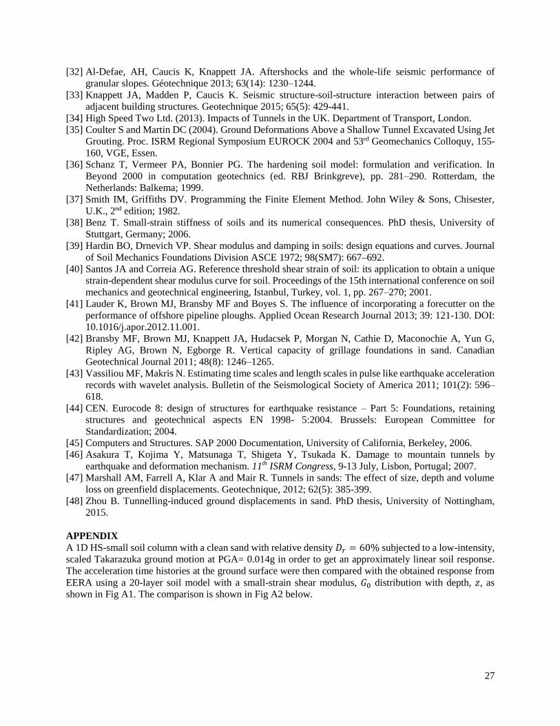
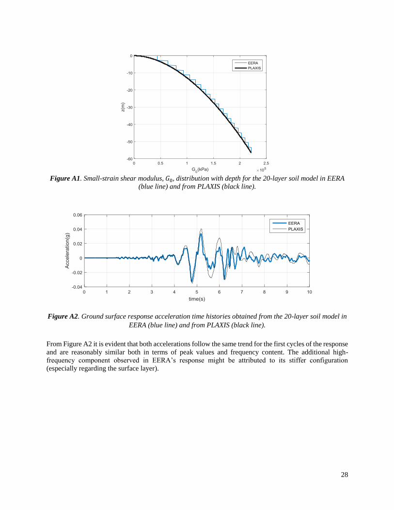
APPENDIX

A 1D HS-small soil column with a clean sand with relative density 𝐷𝑟 = 60% subjected to a low-intensity,

scaled Takarazuka ground motion at PGA= 0.014g in order to get an approximately linear soil response.

The acceleration time histories at the ground surface were then compared with the obtained response from

EERA using a 20-layer soil model with a small-strain shear modulus, 𝐺0 distribution with depth, 𝑧, as

shown in Fig A1. The comparison is shown in Fig A2 below.

28

Figure A1. Small-strain shear modulus, 𝐺0, distribution with depth for the 20-layer soil model in EERA

(blue line) and from PLAXIS (black line).

Figure A2. Ground surface response acceleration time histories obtained from the 20-layer soil model in

EERA (blue line) and from PLAXIS (black line).

From Figure A2 it is evident that both accelerations follow the same trend for the first cycles of the response

and are reasonably similar both in terms of peak values and frequency content. The additional high-

frequency component observed in EERA’s response might be attributed to its stiffer configuration

(especially regarding the surface layer).