THE EFFECTS OF INCOME, WEALTH, AND

THE EFFECTS OF INCOME, WEALTH, AND CAPITAL GAINS TAXATION ON

RISK-TAKING *

J. E. STIGLITZ

I. Introduction, 263.-II. The basic model and some behavioral hypotheses, 264.- III. Wealth tax, 269.- IV. Income taxation, 270. -V. Special treatment of capital gains, 274.- VI. No loss offset, 275.- VII. Welfare implications, 279.

I. INTRODUCTION

In their pioneering article on the effects of taxation on risk- taking, Domar and Musgrave 1 showed that although the imposition of an income tax with full loss-offset might lead to less private risk- taking, total risk-taking would in fact increase.2 If there were no loss-offset, they noted that the amount of risk-taking could either increase or decrease, although the presumption was for the latter. Their analysis rested on individual indifferences curves between risk and mean. The limitations of this kind of analysis are well known.3

The purpose of this note is to investigate the effects on the demand for risky assets of income, capital gains, and wealth taxation, with and without loss-offsets, using a general expected utility maximization model, and to examine the welfare implications of these alternative taxes.

* The research described in this paper was carried out under a grant from the National Science Foundation. After this paper was completed, a paper by J. Mossin, "Taxation and Risk-Taking: An Expected Utility Approach." Economica, XXXV (Feb. 1968), containing some of the results of Sections IV and VI was published. I am indebted to D. Cass and A. Klevorick for their helpful comments.

1. E. Domar and R. Musgrave, "Proportional Income Taxation and Risk-Taking," this Journal, LVI (May 1944), 388-422.

2. For further discussions, see C. Hall, Jr., Fiscal Policy for Stable Growth (New York: Holt, Rinehart and Winston, 1965); R. Musgrave, The Theory of Public Finance (New York: McGraw Hill, 1959); and M. Richter, "Cardinal Utility, Portfolio Selection, and Taxation," Review of Economic Studies, XXVII (June 1960), 152-66.

3. If the measure of risk is variance, then it requires a quadratic utility function, or that the returns from the asset be described by a two-parameter probability distribution. The quadratic utility function has some very peculiar properties, e.g., marginal utility becomes negative at finite incomes and the demand for risky assets decreases with wealth. See J. R. Hicks, "Liquidity," Economic Journal, LXXII (Dec. 1962), 787-802, and K. J. Arrow, Some As- pects of the Theory of Risk Bearing (Helsinki: Yrj6 Johnssonin Saittib, 1965.)

264 QUARTERLY JOURNAL OF ECONOMICS

II. THE BASIC MODEL AND SOME BEHAVIORAL HYPOTHESES

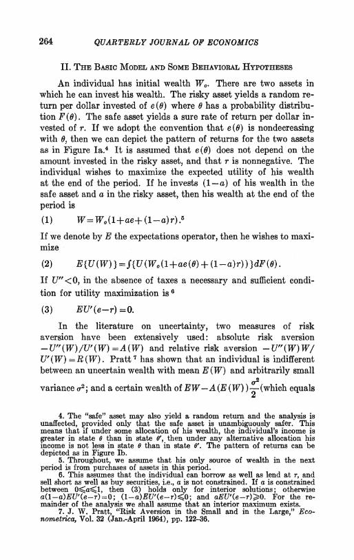
An individual has initial wealth We. There are two assets in which he can invest his wealth. The risky asset yields a random return per dollar invested of e (9) where 9 has a probability distribution F (0). The safe asset yields a sure rate of return per dollar invested of r. If we adopt the convention that e-(9) is nondecreasing with 9, then we can depict the pattern of returns for the two assets as in Figure Ia.4 It is assumed that e (0) does not depend on the amount invested in the risky asset, and that r is nonnegative. The individual wishes to maximize the expected utility of his wealth at the end of the period. If he invests (1-a) of his wealth in the safe asset and a in the risky asset, then his wealth at the end of the period is

(1) W= W0(1+ae+ (1-a)r).5

If we denote by E the expectations operator, then he wishes to maximize

(2) E{U(W)}=-{U(Wo(l+ae(9)+(1-a)r))}dF(9).

If U" <O, in the absence of taxes a necessary and sufficient condition for utility maximization is 6

(3) EU'(e-r)=0.

In the literature on uncertainty, two measures of risk aversion have been extensively used: absolute risk aversion -U"(W)/U'(W) =A(W) and relative risk aversion -U"(W) W U'(W) = R (W). Pratt7 has shown that an individual is indifferent between an uncertain wealth with mean E (W) and arbitrarily small

variance U2; and a certain wealth of EW-A (E (W) ) -2 (which equals

4. The "safe" asset may also yield a random return and the analysis is unaffected, provided only that the safe asset is unambiguously safer. This means that if under some allocation of his wealth, the individual's income is greater in state 0 than in state 0', then under any alternative allocation his income is not less in state 0 than in state 0'. The pattern of returns can be depicted as in Figure Ib.

5. Throughout, we assume that his only source of wealth in the next period is from purchases of assets in this period.

6. This assumes that the individual can borrow as well as lend at r, and sell short as well as buy securities, i.e., a is not constrained. If a is constrained between Oa<1, then (3) holds only for interior solutions; otherwise a(1-a)EU'(e--r)=0; (1-a)EU'(e-r)<O; and aEU'(e-r)>0. For the re- mainder of the analysis we shall assume that an interior maximum exists.

7. J. W. Pratt, "Risk Aversion in the Small and in the Large," Eco- nometrica, Vol. 32 (Jan.-April 1964), pp. 122-36.

EFFECTS OF TAXATION ON RISK-TAKING 265

e (e) r(e)

e FIGURE lB

e (e)

r

a e FIGURE IA

Patterns of Return of Safe and Risky Asset

EW 1-R (E (W) ) j ) ; where a'= o/E (W), the coefficient of vari-

ation). Arrow 8 has argued that: A. Absolute risk aversion decreases as wealth increases. B. Relative risk aversion increases as wealth increases.

These assumptions about the utility function are equivalent to the following assumptions about how the allocation to the risky asset changes as wealth increases:

A.' As wealth increases, more of the risky asset is purchased, i.e., the -risky asset is superior.

8. K. Arrow, op. cit.


B.' As wealth increases, the proportion of one's wealth in the risky asset decreases.

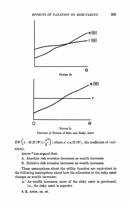
It is easy to show that A and A' and B and B' are equivalent: (3) defines an implicit equation for a in terms of W0. Using the implicit function theorem and integrating by parts, the result is immediate. This result can also be seen graphically as follows. We consider the special case where there are only two states of the world, 01 with probability Pi and 02 with probability P2. If the individual purchases only the safe security, his wealth at the end of the period is represented by the point S in Figure II, with

w(e2)

/

/ TI\

0 w(e,) FIGURE HA

Constant Absolute Risk Aversion

W(01) = W(02) = Wo (1+r). If the individual purchases only the risky asset, his wealth at the end of the period is represented by the point T, with W (01) = Wo (1+e (01) ) and W (02) = Wo (1 +e(02) ), where e (0k) > e(02). Then by allocating different proportions between the two he can obtain any point along the line TS. We have drawn in the same diagram indifference curves for different values of EU, where

(4) EU= piU(W(01) )+p2U(W(02)).

As WO increases, the budget constraint giving different possible. values of W(O1) and W(02) moves outward, but with unchanged slope. The individual maximizes expected utility at the point of


tangency, i.e., where the marginal rate of substitution equals the slope of the budget constraint:

(5) pU'(W (01) e(02)-r

P2U'(W(02)) e(0j)-r

This means that the slope of an Engel curve is given by

(6) dW(2) -U" (W (01) ) /U' (W (01) ) ]A (W (91))

dVdW(01) [-U"((WV(02))/U'(V(02)) ] A (WV(02))

The demand for the risky asset can be written as

(7) aW0o= W (01)-Wo (1 +r) W (02)-Wo (1 +r) e(01)-r e(02)-r

If the risky asset is neither superior nor inferior, then it is easy to see that the Engel curves must have a slope of 450; since with increments in Wo, he purchases only the safe asset, the increments in W(01) and W(02) must be equal:

dW (1) dW(+r) dW(2)

dwo dWo

From equation (5), this means that A(W(1)1) =1 or absolute risk A (W (92))

aversion, -U"/U', is constant. If the risky asset is superior, the Engel curve must have a slope everywhere less than unity; since W(02) <W(01), this means that absolute risk aversion must be de- clining.

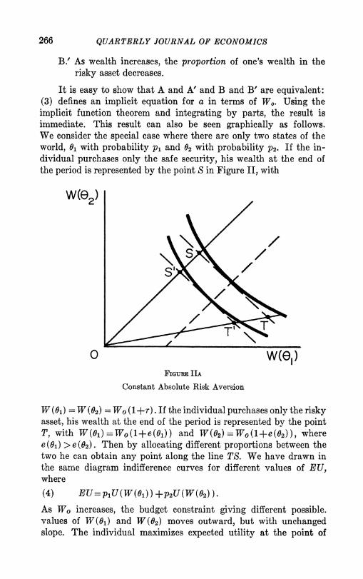
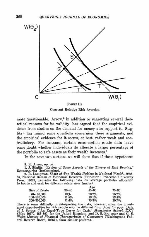
If we divide all terms in equation (7) by WO, we immediately see that if a is to remain constant, then the ratio of W(01) to WO must remain constant and the ratio of W (92) to Wo must remain constant, i.e., W(01) must be proportional to W(02). All Engel curves must be straight lines through the origin, and have unitary elasticity (see Figure IIb), so from equation (6)

dln W (02) -[U" (VW (1) ) W (1) /U' (W (1)) -

din W(91) - U"[U (W(02)) WV(02)/U'(W (02))]

which implies constant relative risk aversion. If a is to decline, as WO increases, the Engel curves must bend upward (towards the "all safe" ray OS). The elasticity must be greater than unity, which implies increasing relative risk aversion. Conversely, if a is to increase as Wo increases, relative risk aversion must be decreasing.

The validity of these testable hypotheses can only be deter- mined empirically. Certainly, the hypothesis that risky assets are not inferior seems reasonable. The second hypothesis is somewhat


w(e2)

0 W(G,) FIGuRE IIB

Constant Relative Risk Aversion

more questionable. Arrow,9 in addition to suggesting several theo- retical reasons for its validity, has argued that the empirical evidence from studies on the demand for money also support it. Stig- litz 1 has raised some questions concerning these arguments, and the empirical evidence for it seems, at best, rather weak and con- tradictory. For instance, certain cross-section estate data leave some doubt whether individuals do allocate a larger percentage of the portfolio to safe assets as their wealth increases.2

In the next two sections we will show that if these hypotheses

9. K. Arrow, op. cit. 1. J. Stiglitz, "Review of Some Aspects of the Theory of Risk Bearing,"

Econometrica (forthcoming). 2. R. Lampman, Share of Top Wealth-Holders in National Wealth, 1922-

56, National Bureau of Economic Research (Princeton: Princeton University Press, 1962), provides the following data on average portfolio allocation to bonds and cash for different estate sizes (males):

Age Size of Estate 30-40 55-60 75-80 70- 80,000 12% 20.2% 26.2%

100-120,000 11.5% 19.1% 23.5% 200-300,000 11.A% 15.3% 20.7%

There is some difficulty in interpreting the data, however, since the investment opportunities for rich people may be different from those for poor. Data of J. Spraos ("An Engel-Type Curve for Cash," Manchester School, XXV (May 1957), 183-89), for the United Kingdom, and D. S. Projector and G. S. Weiss (Survey of Financial Characteristics of Consumers (Washington: Fed- eral Reserve Board, 1966)), show similar patterns.


are correct, then we can make some unambiguous statements about the effects of taxation on risk-taking, independent of the probability distribution of returns for the risky asset, but if these hypotheses are not correct, many of the conclusions of the original Musgrave- Domar analysis may no longer be valid. Our measure of risk-taking is the individual's demand for risky assets; this is simply measured by the fraction of his portfolio devoted to the risky asset. This corresponds to the Domar-Musgrave concept of total (or social) risk-taking. In contrast, there is no obvious corresponding measure of "private risk-taking." One natural measure, which we shall use, is the (subjectively perceived) standard deviation of wealth. In the absence of taxes, this is simply equal to Woao,, where a is the standard deviation of the risky asset.

III. WEALTH TAX

We begin the discussion with an investigation of the effects of the wealth tax, since this is the simplest case to analyze. A proportional wealth tax at the rate t means that wealth at the end of the period is given by

(8) W= Wo (1+ (1-a)r+ae) (1-t).

It should be immediately apparent that changing the tax rate is just equivalent to changing Wo in terms of the effect on risk-taking. Hence we immediately obtain:

Proposition 1 (a). A proportional wealth tax increases, leaves unchanged, or decreases the demand for risky assets as the individual has increasing, constant, or decreasing relative risk aversion.

After tax private risk-taking, P, is given by

P= [E(W-E(W))2]2= [E(Woa(l-t)) (e-Ee))2]?,, = Woa(1-t)o'

where cr2 = E (e - Ee) 2. Whether private risk-taking increases or decreases from an increase in the tax rate depends on whether

dlnP dmna

d In(1-t) d ln(1-t)

But implicit differentiation of the first order condition for expected utility maximization yields

da E {-U"W(e-r)/(1-t)} dt Et-U"(e -r) 2WO}


E {-U"Woa (e-r)2}-EU"Wo(1+r) (e-r)

E{-U"(e-r)2Wo(1-t) } so

dIna WO(1+r)EU"(e-r) d ln(1-t) aE{-U"(e-r)2Wo}

The denominator of the second term on the right-hand side is al-

ways positive. Hence whether -d (1 t) is greater or less than

unity depends on the sign of

-EU"(e-r) =E(-U"/U')U'(e-r) =E(A(W(G)) - A (W (0*) ) U'(e -r) +A (W (0*) ) EU'(e -r)

where 0* is defined by e (0*) = r. The last term equals zero (since utility maximization requires EU'(e-r) = 0). If absolute risk aversion increases with W, in those states of nature where

e (0) > e (0*) = r, A (W (0) ) > A(W (0*) ) , so-}3U"1(e -r) >O0.

Similarly if absolute risk aversion decreases with W,-EU" (e- r) <0. Hence, we have shown: Proposition 1 (b). A proportional wealth tax increases, leaves unchanged, or decreases private risk-taking as the individual has increasing, constant, or decreasing absolute risk aversion.

IV. INCOME TAXATION

The case of income taxation with full loss-offset is only slightly more difficult to analyze. We can write after-tax income, Y, as (9) Y=WO(1-t) [(1-a)r+ae], and his wealth after tax is

W=Wo[1+(1-t) (ae+(1-a)r)].

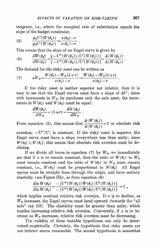
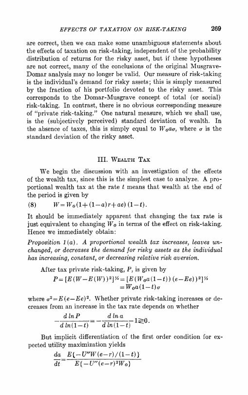
We begin the analysis with the case of only two states of nature. In Figure IIla we have drawn the before-tax budget constraint ST. Income is measured by the distance from, say, T to Wo or S to WO, so an income tax at the rate t reduces the returns from investing in only the safe asset or the risky asset to S' and T', respectively.

The after-tax budget constraint is the line joining T' to S'. It is clearly parallel to ST. Note, however, that a is not constant along a ray through the origin, but along a ray through the point Wo. Thus, it is immediately apparent that in this simple example if individuals have constant or increasing relative risk aversion, or increasing absolute risk aversion, risk-taking will increase. But if


wme2)

S

WO W(el) Fiouis IIIA

Income Tax: Demand for Risky Asset Unchanged

there is decreasing relative risk aversion, just the opposite may occur.

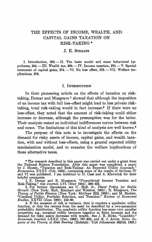
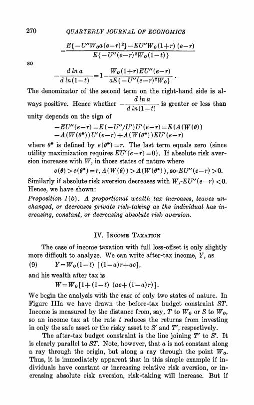
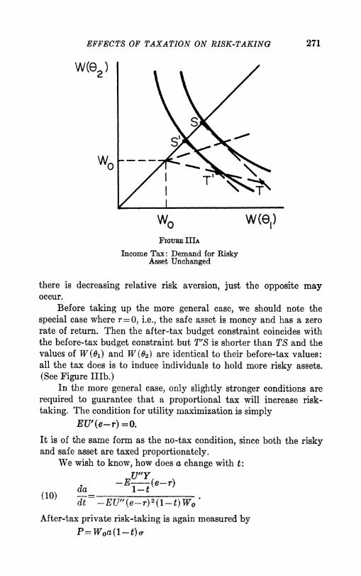
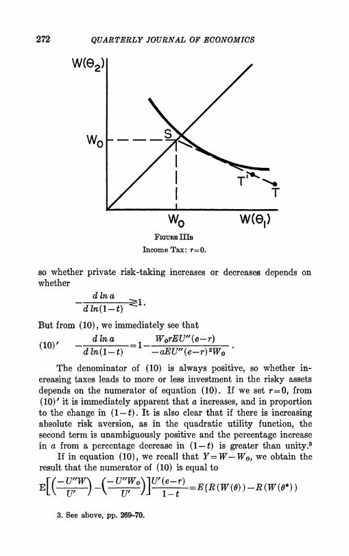
Before taking up the more general case, we should note the special case where r =0, i.e., the safe asset is money and has a zero rate of return. Then the after-tax budget constraint coincides with the before-tax budget constraint but T'S is shorter than TS and the values of W(91) and W(02) are identical to their before-tax values: all the tax does is to induce individuals to hold more risky assets. (See Figure IIIb.)

In the more general case, only slightly stronger conditions are required to guarantee that a proportional tax will increase risk- taking. The condition for utility maximization is simply

EU'(e-r) =0.

It is of the same form as the no-tax condition, since both the risky and safe asset are taxed proportionately.

We wish to know, how does a change with t:

-E (e-r) (10) d--1-

( ct -EU" (e-r) 2 ( 1-t) WO

After-tax private risk-taking is again measured by P=Woa(1-t)a


w(e2)

WO w(e1) FIGURE IIIB

Income Tax: r=0.

so whether private risk-taking increases or decreases depends on whether

d in a

d In(1-t)

But from (10), we immediately see that

(10) d In a WorEU"(e-r) d 1n(1-t) -aEU"(e-r)2WO

The denominator of (10) is always positive, so whether increasing taxes leads to more or less investment in the risky assets depends on the numerator of equation (10). If we set r=O, from (10)' it is immediately apparent that a increases, and in proportion to the change in (1- t). It is also clear that if there is increasing absolute risk aversion, as in the quadratic utility function, the second term is unambiguously positive and the percentage increase in a from a percentage decrease in (1- t) is greater than unity.3

If in equation (10), we recall that Y=W-Wo, we obtain the result that the numerator of (10) is equal to

E 3 S 7=ER(W(0))-R(W(*))

3. See above, pp. 269-70.


-Wo(A(W(0))-A(W(0*)))} U(etr)+{R(W(0*))

-WoA (W(0*))}E P

_ r

where 0* is defined as above. If there is constant or increasing relative risk aversion and constant or decreasing absolute risk aversion, the first term above is unambiguously positive, and by equation (9) the second term is identically zero. Thus, a is increased. But from (10)', if there is decreasing absolute risk aversion, a is increased by a smaller percentage than the percentage decrease in 1- t.

If there is decreasing relative and absolute risk aversion, investment in the risky asset may be unchanged or decreased as the result of the imposition of an income tax. To see this more clearly, consider the following utility function, and assume that the probability of e < 0 is zero:

w

U(W)= A(W-Wo)adW+U(Wo),A>0,a<0. wo

Then, for W> Wo, marginal utility is just U'=A (W-W0)a>0

so absolute risk aversion is U" d n UP -a

->0 UW dW WWo>

and is decreasing, since U" _U a

dW (W-Wo)2<0

while relative risk aversion is -U"W -aW

-U' W-Wo

and is decreasing,

dU"W U = aWo

dW (W= Wo)2O

-U"c -U"Y But since U (W-WO) = , = - a, a constant, it is clear that

the numerator of equation (10) is zero. Thus, for a perfectly well-


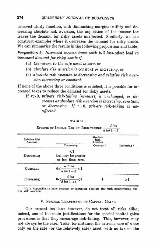
behaved utility function, with diminishing marginal utility and decreasing absolute risk aversion, the imposition of the income tax leaves the demand for risky assets unaffected. Similarly, we can construct examples where it decreases the demand for risky assets. We can summarize the results in the following proposition and table: Proposition 2. Increased income taxes with full loss-offset lead to increased demand for risky assets if

(a) the return to the safe asset is zero, or (b) absolute risk aversion is constant or increasing, or (c) absolute risk aversion is decreasing and relative risk aver-

sion increasing or constant. If none of the above three conditions is satisfied, it is possible for increased taxes to reduce the demand for risky assets.

If r>O, private risk-taking increases, is unchanged, or decreases as absolute risk aversion is increasing, constant, or decreasing. If r = 0, private risk-taking is unaffected.

TABLE I -d 1na

EFFECTS OF INCOME TAX ON RISK-TAKING: d In(1t

Absolute Relative Risk Risk

Aversion Aversion Decreasing Constant * Increasing *

<1 Decreasing but may be greater

or less than zero.

Constant 0<d ma <1 dl1n(1-t)

Increasing 0<d I (1 - <1 1 >1

* It is impossible to have constant or increasing absolute risk with nonincreasing relative risk aversion.

V. SPECIAL TREATMENT OF CAPITAL GAINS

Our present tax laws however, do not treat all risks alike; indeed, one of the main justifications for the special capital gains provisions is that they encourage risk-taking. This, however, may not always be the case. Take, for instance, the extreme case of a tax only on the safe (or the relatively safe) asset, with no tax on the


risky asset. It is easy to show that the demand for the risky asset increases or decreases as

(11) -WOE U"Ir(1 -a) (e - r (1-t) ) +EU'r:::O

and by arguments exactly analogous to those presented above, we can show: Proposition 3(a). A tax on the safe asset alone will increase the demand for the risky asset if there is constant or increasing absolute risk aversion.

Rearranging terms in (11), we obtain the result that the sign of da/dt depends on the sign of

rE { Uj W+1 } U'-WorE (U") (1 +e).

Under limited liability, e > -1, so the second term is unambiguously positive, while the first term is positive if 'relative risk aversion is always less than or equal to unity. Hence, we have shown Proposition 3(b). A tax on the safe asset alone will increase the demand for risky assets if relative risk aversion is less than or equal to unity.

If there is decreasing absolute risk aversion and relative risk aversion is greater than unity it is surely possible for the tax on the safe asset to lead to less rather than more risk-taking. In Sec- tion VII, we shall compare this tax explicitly with a proportional income tax.

VI. No Loss OFFSET

We now examine the effects of no loss-offset provision in an otherwise proportional income tax. After-tax income is given by

WO[l+ae+(1-a)r (1-t)] if e<O. Y=

Wo[1+ (ae+ (1-a)r) (1-t) ] if e>O.

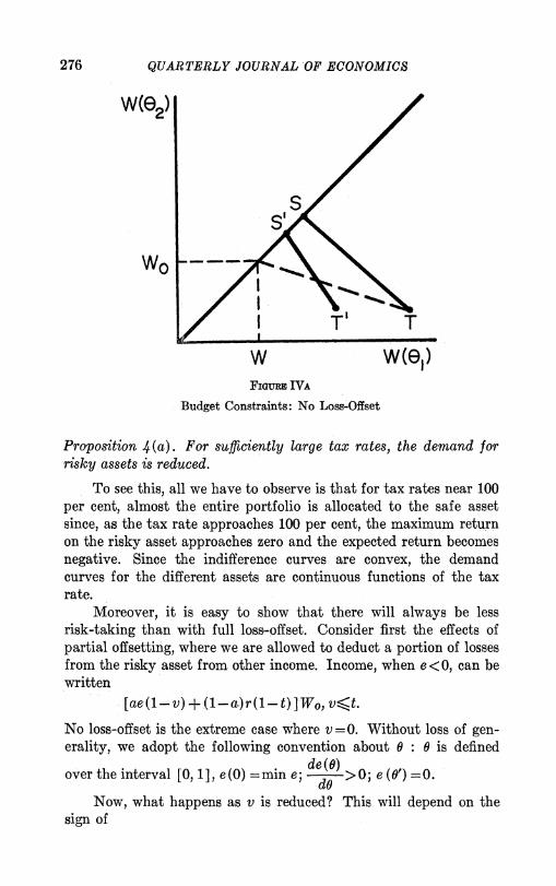
Diagrammatically, the after-tax budget constraint looks as depicted in Figure IVa, if r is greater than zero, or as in Figure IVb, if r= 0. Observe that the value of W (02) if the individual purchases only risky assets is unchanged (i.e., T and T' lie on the same horizontal line). We can see that there is an "income effect" and a "substitution effect," and in the cases discussed in the previous section, these will be of opposite signs, so that the net effect is ambiguous. It is easy to see, however:


W(e2

wo E ~~~T w w(e1) FIGURE IVA

Budget Constraints: No Loss-Offset

Proposition 4(a). For sufficiently large tax rates, the demand for risky assets is reduced.

To see this, all we have to observe is that for tax rates near 100 per cent, almost the entire portfolio is allocated to the safe asset since, as the tax rate approaches 100 per cent, the maximum return on the risky asset approaches zero and the expected return becomes negative. Since the indifference curves are convex, the demand curves for the different assets are continuous functions of the tax rate.

Moreover, it is easy to show that there will always be less risk-taking than with full loss-offset. Consider first the effects of partial offsetting, where we are allowed to deduct a portion of losses from the risky asset from other income. Income, when e <0, can be written

[ae(1-v) + (1-a)r(1-t) ]Wo, v<t.

No loss-offset is the extreme case where v = 0. Without loss of gen- erality, we adopt the following convention about 0 0 is defined

de (0) over the interval [0, 1], e(0) =mine; d >0; e (0') =0.

Now, what happens as v is reduced? This will depend on the sign of


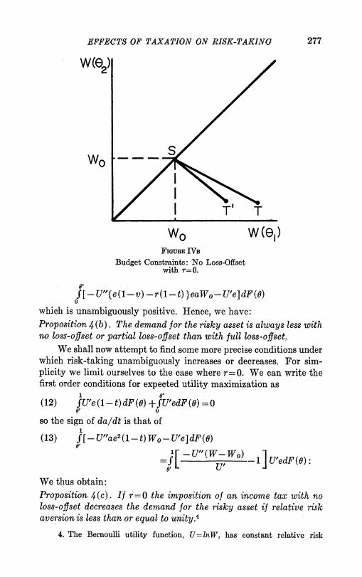
W(e2)

wo C K w

FIGURE IVB

Budget Constraints: No Loss-Offset with r=O.

f[-U"{e(1-v)-r(1-t) }eaWo-U'e]dF(O)

which is unambiguously positive. Hence, we have: Proposition 4 (b). The demand for the risky asset is always less with no loss-offset or partial loss-offset than with full loss-offset.

We shall now attempt to find some more precise conditions under which risk-taking unambiguously increases or decreases. For sim- plicity we limit ourselves to the case where r= 0. We can write the first order conditions for expected utility maximization as

(12) fU'e (1-t) dF (G) +SU'edF () =0 0' ~~~~~0

so the sign of da/dt is that of

(13) f[-U"ae2(1-t)Wo-U'e]dF(O)

-U (W-W ) ]U'edF (0)

We thus obtain: Proposition 4(c). If r= 0 the imposition of an income tax with no loss-offset decreases the demand for the risky asset if relative risk aversion is less than or equal to unity.4

4. The Bernoulli utility function, U=lnW, has constant relative risk


One more condition will now be derived. If we integrate equa- o Y

tion (13) by parts, letting H () =fU'edF () , and a-W we obtain

(14) -fH(O) V +- __W da___ ){dU~Ua

w do

+ {-U (W-W ) 1}H(1).

If there is increasing relative risk aversion the integral expression is negative. Assume that the maximum rate of return is m, so that

U"/W\W- W -U"W W<Wo(m+1); since m/m for

the second term to be negative, all that we require is that relative risk aversion be less than m+1/m at its maximum. If m is 50 per cent, then relative risk aversion need only be less than 3. Thus we have: Proposition 4(d). If r=O, the imposition of an income tax with no loss-offset decreases the demand for the risky asset if there is increasing relative risk aversion, and if the maximum value of relative risk aversion in the relevant region is less than m+l/m, where m is the maximum rate of return.

These results do tend to support the presumption that "social" risk-taking will be reduced by income taxes without loss-offset provisions.

Finally we shall show: Proposition 4(e). If r=0 an income tax with no loss-offset reduces private risk-taking if there is decreasing absolute risk aversion.

1 8' If U2 1 = f e2dF (0) and C22- fe2dF (0) . It is easy to show that private

0' 0 risk-taking decreases if

dBlnra (1-t)221 < ( _ .)2r~ d In (l -t 0 (l0)-21 22

But from (12)

aversion of unity. For small values of W, if the utility function is bounded from below, relative risk aversion must be less than unity, while if the utility function is bounded from above, it must be greater than unity for large values of W. See K. Arrow, op. cit. (This is true provided for large and small W, R(W) is monotonic.)


dIn a of( (-U")e2(1-t)2WO-_U'e(1-t)/a}dF(O)

d ln( -t) -ef'Ute2 (1-t) 2WodF (9) +o0' ( - U") e2WodF (9)

< fJ- U"e2 (1- t) 2WodF (9)

-Of'U"e 2(1- t) 2W0dF (0) - o0'U"e2 WodF(9)

(1-t) 2Bi

(1-t) 2or21+0%22 if U"'>O. But

dA(W) U"' U"E2

dW U' UT2

only if U"'>O.

VII. WELFARE IMPLICATIONS

Even if risk-taking is increased by a given type of tax, it is not clear that such a tax should be adopted: after all, risk-taking is not an end itself. Indeed, there are some who have argued that the stock market pools risk sufficiently effectively that there is no dis- crepancy between social and private risks, and hence no justification for governmental encouragement of risk-taking. It is important to observe, however, that some of the taxes considered may be more effective in obtaining a given end than others. Alternative taxes can be evaluated in terms of (a) losses in expected utility, (b) changes in demands for risky assets, and (c) revenues raised in each state of nature. Note that the last is much more stringent than comparisons simply between average revenues; two taxes may have the same expected revenue, but differ in the revenue they provide in different states of nature.

In this section we shall analyze the welfare implications of the preferential treatment of capital gains. To do this, we shall look at the polar case where risky assets are completely exempt from taxation, and compare its effects with those of alternative taxes.

A. Comparison of taxes with equal loss of expected utility.

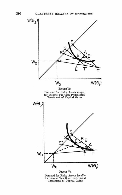
First, we compare the tax on the safe asset only with a proportional income tax. From Figures Va and Vb it is clear that the demand for risky assets may actually be larger with an income tax than with a tax on the safe asset only. ST represents the before-tax budget constraint, S'T' the after-tax budget constraint for the income tax, S"T the after-tax budget constraint for the tax on the safe asset only. We have already noted that if the after-tax income


W(o)

FIGURE YB Demand for Risky Assets Larger for Income Tax than Preferential

Treatment of Capital Gains

w(e2)

wo w(e1) FIGURE VA

Demand for Risky Assets Smaller for Income Tax than Preferential

Treatment of Capital Gains


wMe2) S

WoO wo w(e)

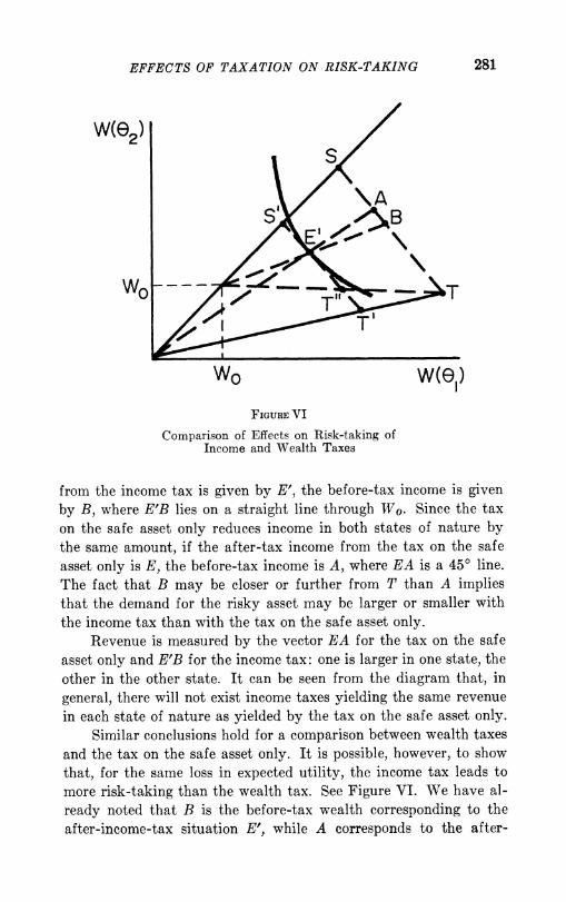
FIGURE VI

Comparison of Effects on Risk-taking of Income and Wealth Taxes

from the income tax is given by E', the before-tax income is given by B, where E'B lies on a straight line through Wo. Since the tax on the safe asset only reduces income in both states of nature by the same amount, if the after-tax income from the tax on the safe asset only is E, the before-tax income is A, where EA is a 450 line. The fact that B may be closer or further from T than A implies that the demand for the risky asset may be larger or smaller with the income tax than with the tax on the safe asset only.

Revenue is measured by the vector EA for the tax on the safe asset only and E'B for the income tax: one is larger in one state, the other in the other state. It can be seen from the diagram that, in general, there will not exist income taxes yielding the same revenue in each state of nature as yielded by the tax on the safe asset only.

Similar conclusions hold for a comparison between wealth taxes and the tax on the safe asset only. It is possible, however, to show that, for the same loss in expected utility, the income tax leads to more risk-taking than the wealth tax. See Figure VI. We have already noted that B is the before-tax wealth corresponding to the after-income-tax situation E', while A corresponds to the after-


wealth-tax situation E', where EA lies on a straight line through the origin. But since A is closer to S than B, the result is immediate.

B. Comparison of taxes of equal revenue.

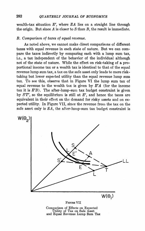
As noted above, we cannot make direct comparisons of different taxes with equal revenue in each state of nature. But we can compare the taxes indirectly by comparing each with a lump sum tax, i.e., a tax independent of the behavior of the individual although not of the state of nature. While the effect on risk-taking of a proportional income tax or a wealth tax is identical to that of the equal revenue lump sum tax, a tax on the safe asset only leads to more risk- taking but lower expected utility than the equal revenue lump sum tax. To see this, observe that in Figure VI the lump sum tax of equal revenue to the wealth tax is given by E'A (for the income tax it is E'B). The after-lump-sum tax budget constraint is given by S'T', so the equilibrium is still at E', and hence the taxes are equivalent in their effect on the demand for risky assets and on expected utility. In Figure VII, since the revenue from the tax on the safe asset only is EA, the after-lump-sum tax budget constraint is

w(e2)

S L E A

.,___L~~~LL

w(e1) FIGURE VII

Comparison of Effects on Expected Utility of Tax on Safe Asset

and Equal Revenue Lump Sum Tax


LL, and the equilibrium is given by E', which implies a higher demand for risky assets but at the cost of a lower level of utility for the tax on the safe asset than for the equal revenue lump sum tax.

The important point to observe is that even if one wished to encourage greater risk-taking, and even if preferential treatment of capital gains did this effectively, it is not clear that preferential treatment of capital gains is the most desirable way of encouraging risk-taking.

COWLES FOUNDATION YALE UNIVERSITY

Documents

THE EFFECTS OF INCOME, WEALTH, AND