The Fourier Transform (What you need to know)wjh/teaching/Fourier/documents/booklet.pdf · The Fourier Transform (What you need to know) ... This slightly odd convention and is to

FOURIER BOOKLET -1

School of Physics

TH

E

U N I V E RS

I TY

OF

ED I N B U

RG

H

The Fourier Transform(What you need to know)

Mathematical Background for:

Senior Honours Modern OpticsSenior Honours Digital Image AnalysisSenior Honours Optical Laboratory ProjectsMSc Theory of Image Processing

Session: 2007-2008Version: 3.1.1

School of Physics Fourier Transform Revised: 10 September 2007

FOURIER BOOKLET -1

Contents1 Introduction 2

1.1 Notation . . . . . . . . . . . . . . . . . . . . . . . . . . . . . . . . . . . . . . 2

2 The Fourier Transform 32.1 Properties of the Fourier Transform . . . . . . . . . . . . . . . . . . . . . . . 42.2 Two Dimensional Fourier Transform . . . . . . . . . . . . . . . . . . . . . . . 52.3 The Three-Dimensional Fourier Transform . . . . . . . . . . . . . . . . . . . . 6

3 Dirac Delta Function 73.1 Properties of the Dirac Delta Function . . . . . . . . . . . . . . . . . . . . . . 83.2 The Infinite Comb . . . . . . . . . . . . . . . . . . . . . . . . . . . . . . . . . 9

4 Symmetry Conditions 104.1 One-Dimensional Symmetry . . . . . . . . . . . . . . . . . . . . . . . . . . . 114.2 Two-Dimensional Symmetry . . . . . . . . . . . . . . . . . . . . . . . . . . . 12

5 Convolution of Two Functions 135.1 Simple Properties . . . . . . . . . . . . . . . . . . . . . . . . . . . . . . . . . 145.2 Two Dimensional Convolution . . . . . . . . . . . . . . . . . . . . . . . . . . 14

6 Correlation of Two Functions 156.1 Autocorrelation . . . . . . . . . . . . . . . . . . . . . . . . . . . . . . . . . . 16

7 Questions 177.1 The sinc() function . . . . . . . . . . . . . . . . . . . . . . . . . . . . . . . . 177.2 Rectangular Aperture . . . . . . . . . . . . . . . . . . . . . . . . . . . . . . . 187.3 Gaussians . . . . . . . . . . . . . . . . . . . . . . . . . . . . . . . . . . . . . 197.4 Differentials . . . . . . . . . . . . . . . . . . . . . . . . . . . . . . . . . . . . 217.5 Delta Functions . . . . . . . . . . . . . . . . . . . . . . . . . . . . . . . . . . 227.6 Sines and Cosines . . . . . . . . . . . . . . . . . . . . . . . . . . . . . . . . . 237.7 Comb Function . . . . . . . . . . . . . . . . . . . . . . . . . . . . . . . . . . 247.8 Convolution Theorm . . . . . . . . . . . . . . . . . . . . . . . . . . . . . . . 257.9 Correlation Theorm . . . . . . . . . . . . . . . . . . . . . . . . . . . . . . . . 277.10 Auto-Correlation . . . . . . . . . . . . . . . . . . . . . . . . . . . . . . . . . 28


-2 FOURIER BOOKLET

1 IntroductionFourier Transform theory is essential to many areas of physics including acoustics and signalprocessing, optics and image processing, solid state physics, scattering theory, and the moregenerally, in the solution of differential equations in applications as diverse as weather model-ing to quantum field calculations. The Fourier Transform can either be considered as expansionin terms of an orthogonal bases set (sine and cosine), or a shift of space from real space to re-ciprocal space. Actually these two concepts are mathematically identical although they areoften used in very different physical situations.The aim of this booklet is to cover the Fourier Theory required primarily for the

• Junior Honours course OPTICS.

• Senior Honours course MODERN OPTICS1 and DIGITAL IMAGE ANALYSIS

• Geoscience MSc course THEORY OF IMAGE PROCESSING .

It also contains examples from acoustics and solid state physics so should be generally usefulfor these courses. The mathematical results presented in this booklet will be used in the abovecourses and they are expected to be known.There are a selection of tutorial style questions with full solutions at the back of the booklet.These contain a range of examples and mathematical proofs, some of which are fairly difficult,particularly the parts in italic. The mathematical proofs are not in themselves an examinal partof the lecture courses, but the results and techniques employed are.Further details of Fourier Transforms can be found in “Introduction to the Fourier Transformand its Applications” by Bracewell and “Mathematical Methods for Physics and Engineering”by Riley, Hobson & Bence.

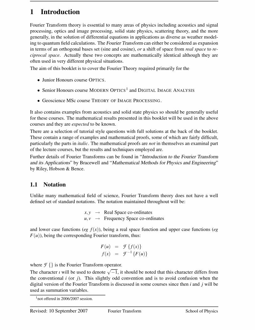
1.1 NotationUnlike many mathematical field of science, Fourier Transform theory does not have a welldefined set of standard notations. The notation maintained throughout will be:

x,y → Real Space co-ordinatesu,v → Frequency Space co-ordinates

and lower case functions (eg f (x)), being a real space function and upper case functions (egF(u)), being the corresponding Fourier transform, thus:

F(u) = F { f (x)}f (x) = F −1 {F(u)}

where F {} is the Fourier Transform operator.The character ı will be used to denote

√−1, it should be noted that this character differs from

the conventional i (or j). This slightly odd convention and is to avoid confusion when thedigital version of the Fourier Transform is discussed in some courses since then i and j will beused as summation variables.

1not offered in 2006/2007 session.

Revised: 10 September 2007 Fourier Transform School of Physics

http://www.ph.ed.ac.uk/~wjh/teaching/optics/

http://www.ph.ed.ac.uk/~wjh/teaching/mo/

http://www.ph.ed.ac.uk/~wjh/teaching/dia/

http://www.ph.ed.ac.uk/~wjh/teaching/toip/

FOURIER BOOKLET -3

-0.4

-0.2

0

0.2

0.4

0.6

0.8

1

-10 -5 0 5 10

sinc(x)

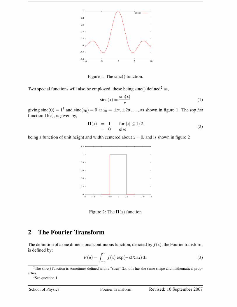
Figure 1: The sinc() function.

Two special functions will also be employed, these being sinc() defined2 as,

sinc(x) =sin(x)

x (1)

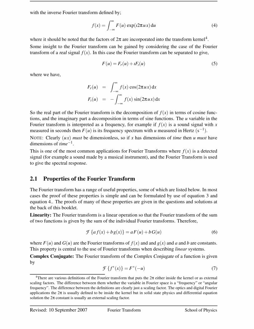
giving sinc(0) = 13 and sinc(x0) = 0 at x0 = ±π, ±2π, . . ., as shown in figure 1. The top hatfunction Π(x), is given by,

Π(x) = 1 for |x| ≤ 1/2= 0 else (2)

being a function of unit height and width centered about x = 0, and is shown in figure 2

0

0.2

0.4

0.6

0.8

1

1.2

-2 -1.5 -1 -0.5 0 0.5 1 1.5 2

Figure 2: The Π(x) function

2 The Fourier TransformThe definition of a one dimensional continuous function, denoted by f (x), the Fourier transformis defined by:

F(u) =

Z ∞

−∞f (x) exp(−ı2πux)dx (3)

2The sinc() function is sometimes defined with a “stray” 2π, this has the same shape and mathematical prop-erties.

3See question 1


-4 FOURIER BOOKLET

with the inverse Fourier transform defined by;

f (x) =

Z ∞

−∞F(u) exp(ı2πux)du (4)

where it should be noted that the factors of 2π are incorporated into the transform kernel4.Some insight to the Fourier transform can be gained by considering the case of the Fouriertransform of a real signal f (x). In this case the Fourier transform can be separated to give,

F(u) = Fr(u)+ ıFı(u) (5)

where we have,

Fr(u) =Z ∞

−∞f (x) cos(2πux)dx

Fı(u) = −Z ∞

−∞f (x) sin(2πux)dx

So the real part of the Fourier transform is the decomposition of f (x) in terms of cosine func-tions, and the imaginary part a decomposition in terms of sine functions. The u variable in theFourier transform is interpreted as a frequency, for example if f (x) is a sound signal with xmeasured in seconds then F(u) is its frequency spectrum with u measured in Hertz (s−1).NOTE: Clearly (ux) must be dimensionless, so if x has dimensions of time then u must havedimensions of time−1.This is one of the most common applications for Fourier Transforms where f (x) is a detectedsignal (for example a sound made by a musical instrument), and the Fourier Transform is usedto give the spectral response.

2.1 Properties of the Fourier TransformThe Fourier transform has a range of useful properties, some of which are listed below. In mostcases the proof of these properties is simple and can be formulated by use of equation 3 andequation 4.. The proofs of many of these properties are given in the questions and solutions atthe back of this booklet.Linearity: The Fourier transform is a linear operation so that the Fourier transform of the sumof two functions is given by the sum of the individual Fourier transforms. Therefore,

F {a f (x)+bg(x)} = aF(u)+bG(u) (6)

where F(u) and G(u) are the Fourier transforms of f (x) and and g(x) and a and b are constants.This property is central to the use of Fourier transforms when describing linear systems.Complex Conjugate: The Fourier transform of the Complex Conjugate of a function is givenby

F { f ∗(x)} = F∗(−u) (7)4There are various definitions of the Fourier transform that puts the 2π either inside the kernel or as external

scaling factors. The difference between them whether the variable in Fourier space is a “frequency” or “angularfrequency”. The difference between the definitions are clearly just a scaling factor. The optics and digital Fourierapplications the 2π is usually defined to be inside the kernel but in solid state physics and differential equationsolution the 2π constant is usually an external scaling factor.


FOURIER BOOKLET -5

where F(u) is the Fourier transform of f (x).Forward and Inverse: We have that

F {F(u)} = f (−x) (8)

so that if we apply the Fourier transform twice to a function, we get a spatially reversed versionof the function. Similarly with the inverse Fourier transform we have that,

F −1 { f (x)} = F(−u) (9)

so that the Fourier and inverse Fourier transforms differ only by a sign.Differentials: The Fourier transform of the derivative of a functions is given by

F{

d f (x)dx

}

= ı2πuF(u) (10)

and the second derivative is given by

F{

d2 f (x)dx2

}

= −(2πu)2 F(u) (11)

This property will be used in the DIGITAL IMAGE ANALYSIS and THEORY OF IMAGE PRO-CESSING course to form the derivative of an image.Power Spectrum: The Power Spectrum of a signal is defined by the modulus square of theFourier transform, being |F(u)|2. This can be interpreted as the power of the frequency com-ponents. Any function and its Fourier transform obey the condition that

Z ∞

−∞| f (x)|2 dx =

Z ∞

−∞|F(u)|2 du (12)

which is frequently known as Parseval’s Theorem5. If f (x) is interpreted at a voltage, thenthis theorem states that the power is the same whether measured in real (time), or Fourier(frequency) space.

2.2 Two Dimensional Fourier TransformSince the three courses covered by this booklet use two-dimensional scalar potentials or imageswe will be dealing with two dimensional function. We will define the two dimensional Fouriertransform of a continuous function f (x,y) by,

F(u,v) =

Z Z

f (x,y) exp(−ı2π(ux+ vy)) dxdy (13)

with the inverse Fourier transform defined by;

f (x,y) =Z Z

F(u,v) exp(ı2π(ux+ vy)) dudv (14)

where the limits of integration are taken from −∞ → ∞6

5Strictly speaking Parseval’s Theorem applies to the case of Fourier series, and the equivalent theorem forFourier transforms is correctly, but less commonly, known as Rayleigh’s theorem

6Unless otherwise specified all integral limits will be assumed to be from −∞ → ∞


-6 FOURIER BOOKLET

Again for a real two dimensional function f (x,y), the Fourier transform can be considered asthe decomposition of a function into its sinusoidal components. If f (x,y) is considered to be animage with the “brightness” of the image at point (x0,y0) given by f (x0,y0), then variables x,yhave the dimensions of length. In Fourier space the variables u,v have therefore the dimensionsof inverse length, which is interpreted as Spatial Frequency.NOTE: Typically x and y are measured in mm so that u and v have are in units of mm−1 alsoreferred to at lines per mm.The Fourier transform can then be taken as being the decomposition of the image into two di-mensional sinusoidal spatial frequency components. This property will be examined in greaterdetail the relevant courses.The properties of one the dimensional Fourier transforms covered in the previous section con-vert into two dimensions. Clearly the derivatives then become

F{

∂ f (x,y)∂x

}

= ı2πuF(u,v) (15)

and withF{

∂ f (x,y)∂y

}

= ı2πvF(u,v) (16)

yielding the important result that,

F {∇2 f (x,y)}

= −(2πw)2 F(u,v) (17)

where we have that w2 = u2 + v2. So that taking the Laplacian of a function in real space isequivalent to multiplying its Fourier transform by a circularly symmetric quadratic of −4π2w2.The two dimensional Fourier Transform F(u,v), of a function f (x,y) is a separable operation,and can be written as,

F(u,v) =

Z

P(u,y)exp(−ı2πvy)dy (18)

whereP(u,y) =

Z

f (x,y) exp(−ı2πux)dx (19)

where P(u,y) is the Fourier Transform of f (x,y) with respect to x only. This property ofseparability will be considered in greater depth with regards to digital images and will lead toan implementation of two dimensional discrete Fourier Transforms in terms of one dimensionalFourier Transforms.

2.3 The Three-Dimensional Fourier TransformIn the three dimensional case we have a function f (~r) where ~r = (x,y,z), then the three-dimensional Fourier Transform

F(~s) =

Z Z Z

f (~r) exp(−ı2π~r .~s) d~r

where~s = (u,v,w) being the three reciprocal variables each with units length−1. Similarly theinverse Fourier Transform is given by

f (~r) =

Z Z Z

F(~s) exp(ı2π~r .~s) d~s


FOURIER BOOKLET -7

This is used extensively in solid state physics where the three-dimensional Fourier Transformof a crystal structures is usually called Reciprocal Space7.The three-dimensional Fourier Transform is again separable into one-dimensional Fourier Trans-form. This property is independent of the dimensionality and multi-dimensional Fourier Trans-form can be formulated as a series of one dimensional Fourier Transforms.

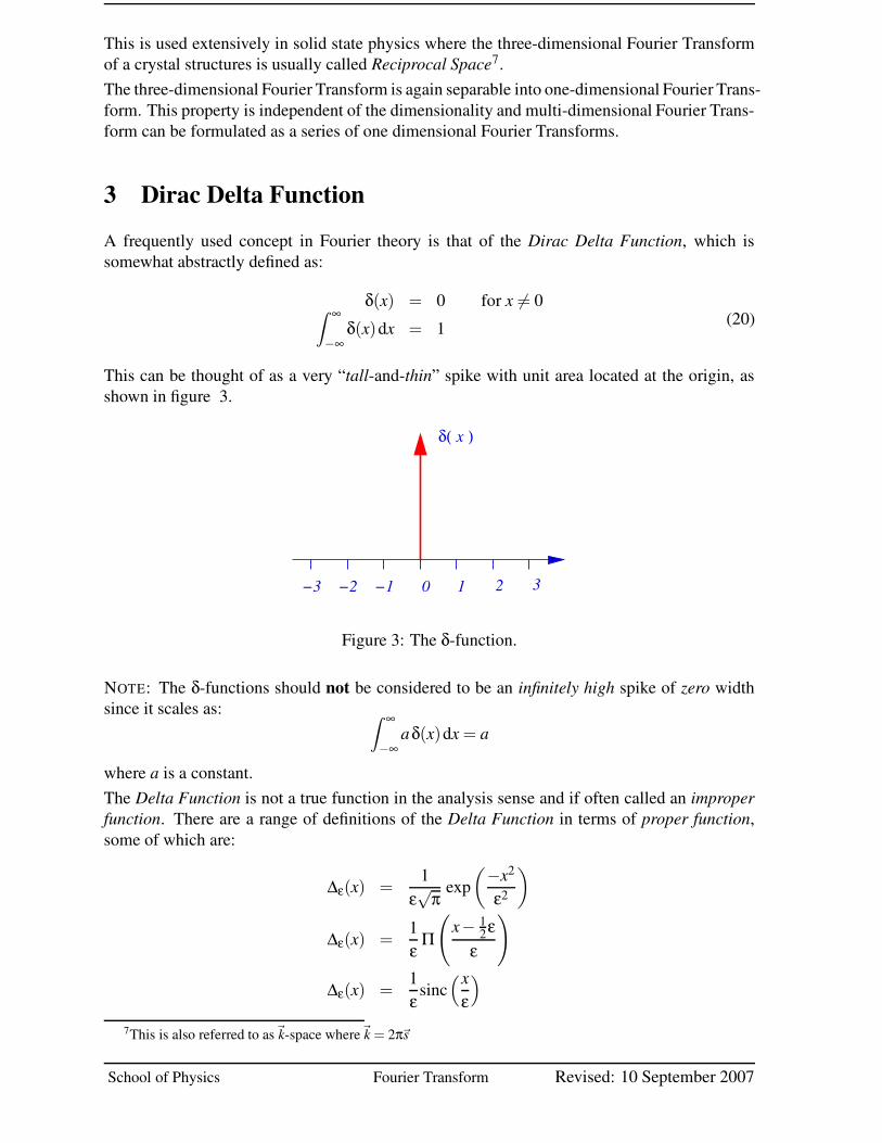
3 Dirac Delta FunctionA frequently used concept in Fourier theory is that of the Dirac Delta Function, which issomewhat abstractly defined as:

δ(x) = 0 for x 6= 0Z ∞

−∞δ(x)dx = 1 (20)

This can be thought of as a very “tall-and-thin” spike with unit area located at the origin, asshown in figure 3.

−3 −2 0−1 1 2 3

xδ( )

Figure 3: The δ-function.

NOTE: The δ-functions should not be considered to be an infinitely high spike of zero widthsince it scales as:

Z ∞

−∞aδ(x)dx = a

where a is a constant.The Delta Function is not a true function in the analysis sense and if often called an improperfunction. There are a range of definitions of the Delta Function in terms of proper function,some of which are:

∆ε(x) =1

ε√

πexp(−x2

ε2

)

∆ε(x) =1ε

Π

(

x− 12ε

ε

)

∆ε(x) =1ε

sinc(x

ε

)

7This is also referred to as~k-space where~k = 2π~s


-8 FOURIER BOOKLET

being the Gaussian, Top-Hat and Sinc approximations respectively. All of these expressionshave the property that,

Z ∞

−∞∆ε(x)dx = 1 ∀ε (21)

and we may form the approximation that,

δ(x) = limε→0

∆ε(x) (22)

which can be interpreted as making any of the above approximations ∆ε(x) a very “tall-andthin”spike with unit area.In the field of optics and imaging, we are dealing with two dimensional distributions, so it isespecially useful to define the Two Dimensional Dirac Delta Function, as,

δ(x,y) = 0 for x 6= 0 & y 6= 0Z Z

δ(x,y)dxdy = 1 (23)

which is the two dimensional version of the δ(x) function defined above, and in particular:

δ(x,y) = δ(x)δ(y). (24)

This is the two dimensional analogue of the impulse function used in signal processing. Interms of an imaging system, this function can be considered as a single bright spot in the centreof the field of view, for example a single bright star viewed by a telescope.

3.1 Properties of the Dirac Delta FunctionSince the Dirac Delta Function is used extensively, and has some useful, and slightly perculiarproperties, it is worth considering these are this point. For a function f (x), being integrable,then we have that

Z ∞

−∞δ(x) f (x)dx = f (0) (25)

which is often taken as an alternative definition of the Delta function. This says that integralof any function multiplied by a δ-function located about zero is just the value of the functionat zero. This concept can be extended to give the Shifting Property, again for a function f (x),giving,

Z ∞

−∞δ(x−a) f (x)dx = f (a) (26)

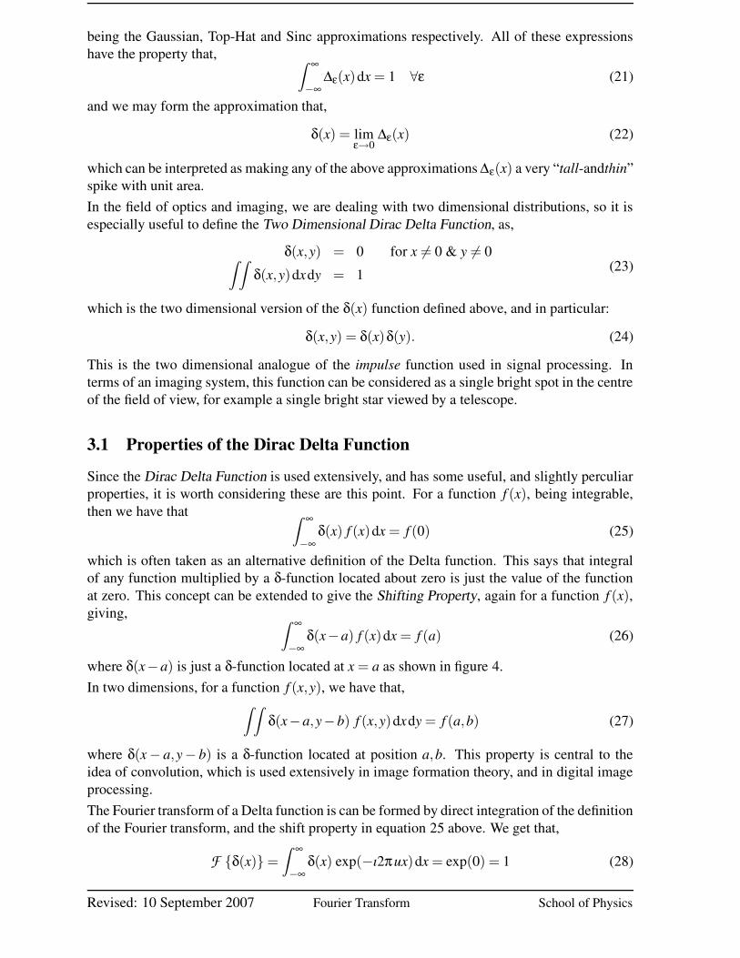
where δ(x−a) is just a δ-function located at x = a as shown in figure 4.In two dimensions, for a function f (x,y), we have that,

Z Z

δ(x−a,y−b) f (x,y)dxdy = f (a,b) (27)

where δ(x − a,y− b) is a δ-function located at position a,b. This property is central to theidea of convolution, which is used extensively in image formation theory, and in digital imageprocessing.The Fourier transform of a Delta function is can be formed by direct integration of the definitionof the Fourier transform, and the shift property in equation 25 above. We get that,

F {δ(x)} =

Z ∞

−∞δ(x) exp(−ı2πux)dx = exp(0) = 1 (28)


FOURIER BOOKLET -9

f(x)f(a)

xa0

Figure 4: Shifting property of the δ-function.

and then by the Shifting Theorem, equation 26, we get that,

F {δ(x−a)} = exp(−ı2πau) (29)

so that the Fourier transform of a shifted Delta Function is given by a phase ramp. It should benoted that the modulus squared of equation 29 is

|F {δ(x−a)}|2 = |exp(−ı2πau)|2 = 1

saying that the power spectrum a Delta Function is a constant independent of its location inreal space.Now noting that the Fourier transform is a linear operation, then if we consider two DeltaFunction located at ±a, then from equation 29 the Fourier transform gives,

F {δ(x−a)+δ(x+a)} = exp(−ı2πau)+ exp(ı2πau) = 2cos(2πau) (30)

while if we have the Delta Function at x = −a as negative, then we also have that,

F {δ(x−a)−δ(x+a)} = exp(−ı2πau)− exp(ı2πau) = −2ısin(2πau). (31)

Noting the relations between forward and inverse Fourier transform we then get the two usefulresults that

F {cos(2πax)} =12 [δ(u−a)+δ(u+a)] (32)

and thatF {sin(2πax)} =

12ı [δ(u−a)−δ(u+a)] (33)

So that the Fourier transform of a cosine or sine function consists of a single frequency givenby the period of the cosine or sine function as would be expected.

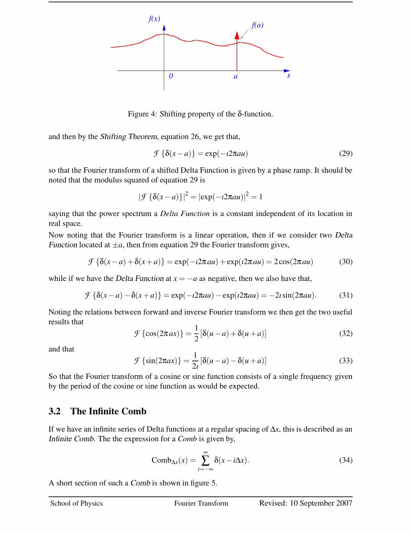
3.2 The Infinite CombIf we have an infinite series of Delta functions at a regular spacing of ∆x, this is described as anInfinite Comb. The the expression for a Comb is given by,

Comb∆x(x) =∞

∑i=−∞

δ(x− i∆x). (34)

A short section of such a Comb is shown in figure 5.


-10 FOURIER BOOKLET

x 2 x 3 x 4 x− x−2 x−3 x−4 x ∆∆∆∆∆ ∆∆∆

x∆

x0

Figure 5: Infinite Comb with separation ∆x

Since the Fourier transform is a linear operation then the Fourier transform of the infinite combis the sum of the Fourier transforms of shifted Delta functions, which from equation (29) gives,

F {Comb∆x(x)} =∞

∑i=−∞

exp(−ı2π i∆xu) (35)

Now the exponential term,

exp(−ı2πi∆xu) = 1 when 2π∆xu = 2πn

so that:∞

∑i=−∞

exp(−ı2π i∆xu) → ∞ when u = n∆x

= 0 else

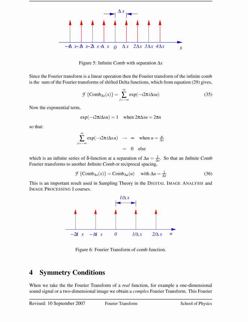
which is an infinite series of δ-function at a separation of ∆u = 1∆x . So that an Infinite Comb

Fourier transforms to another Infinite Comb or reciprocal spacing,

F {Comb∆x(x)} = Comb∆u(u) with ∆u = 1∆x (36)

This is an important result used in Sampling Theory in the DIGITAL IMAGE ANALYSIS andIMAGE PROCESSING I courses.

∆ ∆ ∆ ∆

∆

0 u−2/ x −1/ x 1/ x 2/ x

1/ x

Figure 6: Fourier Transform of comb function.

4 Symmetry ConditionsWhen we take the the Fourier Transform of a real function, for example a one-dimensionalsound signal or a two-dimensional image we obtain a complex Fourier Transform. This Fourier


FOURIER BOOKLET -11

Transform has special symmetry properties that are essential when calculating and/or manip-ulating Fourier Transforms. This section it of the booklet is mainly aimed at the DIGITALIMAGE ANALYSIS and THEORY OF IMAGE PROCESSING courses that make extensive use ofthese symmetry conditions.

4.1 One-Dimensional SymmetryFirstly consider the case of a one dimensional real function f (x), with a Fourier transform ofF(u). Since f (x) is real then from previous we can write

F(u) = Fr(u)+ ıFı(u)

where the real and imaginary parts are given by the cosine and sine transforms to be

Fr(u) =

Z

f (x) cos(2πux)dx

Fı(u) = −Z

f (x) sin(2πux)dx(37)

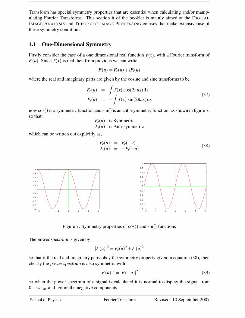
now cos() is a symmetric function and sin() is an anti-symmetric function, as shown in figure 7,so that:

Fr(u) is SymmetricFı(u) is Anti-symmetric

which can be written out explicitly as,

Fr(u) = Fr(−u)Fı(u) = −Fı(−u)

(38)

-1

-0.8

-0.6

-0.4

-0.2

0

0.2

0.4

0.6

0.8

1

-6 -4 -2 0 2 4 6-1

-0.8

-0.6

-0.4

-0.2

0

0.2

0.4

0.6

0.8

1

-6 -4 -2 0 2 4 6

Figure 7: Symmetry properties of cos() and sin() functions

The power spectrum is given by

|F(u)|2 = Fr(u)2 +Fı(u)2

so that if the real and imaginary parts obey the symmetry property given in equation (38), thenclearly the power spectrum is also symmetric with

|F(u)|2 = |F(−u)|2 (39)

so when the power spectrum of a signal is calculated it is normal to display the signal from0 → umax and ignore the negative components.


-12 FOURIER BOOKLET

4.2 Two-Dimensional SymmetryIn two dimensional we have a real image f (x,y), and then as above the Fourier transform ofthis image can be written as,

F(u,v) = Fr(u,v)+ ıFı(u,v) (40)

where after expansion of the exp() functions into cos() and sin() functions we get that

Fr(u,v) =

Z Z

f (x,y) [cos(2πux) cos(2πvy)− sin(2πux) sin(2πvy)] dxdy

and that;

Fı(u,v) =Z Z

f (x,y) [cos(2πux) sin(2πvy)+ sin(2πux) cos(2πvy)] dxdy

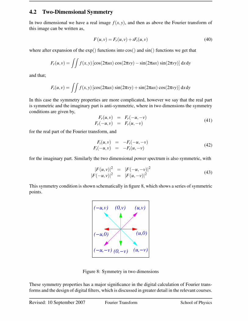
In this case the symmetry properties are more complicated, however we say that the real partis symmetric and the imaginary part is anti-symmetric, where in two dimensions the symmetryconditions are given by,

Fr(u,v) = Fr(−u,−v)Fr(−u,v) = Fr(u,−v) (41)

for the real part of the Fourier transform, and

Fı(u,v) = −Fı(−u,−v)Fı(−u,v) = −Fı(u,−v) (42)

for the imaginary part. Similarly the two dimensional power spectrum is also symmetric, with

|F(u,v)|2 = |F(−u,−v)|2|F(−u,v)|2 = |F(u,−v)|2 (43)

This symmetry condition is shown schematically in figure 8, which shows a series of symmetricpoints.

(−u,v) (0,v) (u,v)

(u,0)

(u,−v)(0,−v)(−u,−v)

(−u,0)

Figure 8: Symmetry in two dimensions

These symmetry properties has a major significance in the digital calculation of Fourier trans-forms and the design of digital filters, which is discussed in greater detail in the relevant courses.


FOURIER BOOKLET -13

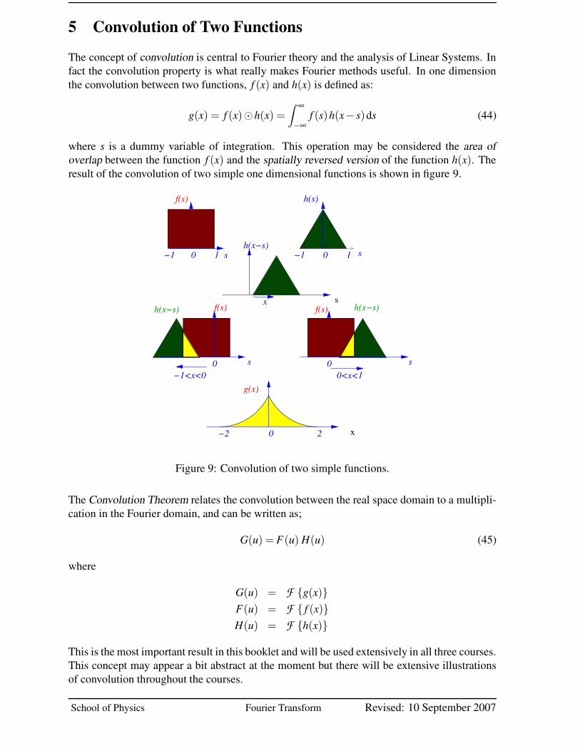
5 Convolution of Two FunctionsThe concept of convolution is central to Fourier theory and the analysis of Linear Systems. Infact the convolution property is what really makes Fourier methods useful. In one dimensionthe convolution between two functions, f (x) and h(x) is defined as:

g(x) = f (x)�h(x) =Z ∞

−∞f (s)h(x− s)ds (44)

where s is a dummy variable of integration. This operation may be considered the area ofoverlap between the function f (x) and the spatially reversed version of the function h(x). Theresult of the convolution of two simple one dimensional functions is shown in figure 9.

x

s

h(s)

h(x−s)

f(s)

f(s) h(x−s)h(x−s) f(s)

0<x<10 s

−1<x<00 s

−1 1 s0 −1 0 1 s

x

−2 0 2

g(x)

Figure 9: Convolution of two simple functions.

The Convolution Theorem relates the convolution between the real space domain to a multipli-cation in the Fourier domain, and can be written as;

G(u) = F(u) H(u) (45)

where

G(u) = F {g(x)}F(u) = F { f (x)}H(u) = F {h(x)}

This is the most important result in this booklet and will be used extensively in all three courses.This concept may appear a bit abstract at the moment but there will be extensive illustrationsof convolution throughout the courses.


-14 FOURIER BOOKLET

5.1 Simple PropertiesThe convolution is a linear operation which is distributative, so that for three functions f (x),g(x) and h(x) we have that

f (x)� (g(x)�h(x)) = ( f (x)�g(x))�h(x) (46)and commutative, so that

f (x)�h(x) = h(x)� f (x) (47)

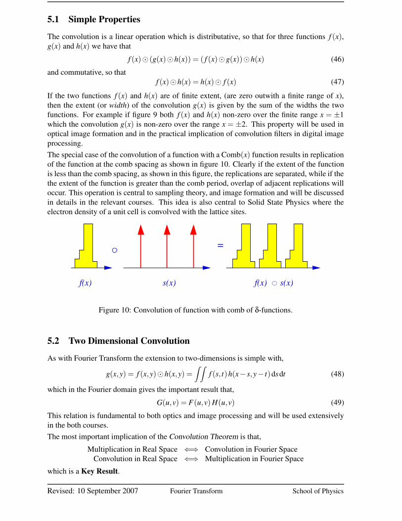
If the two functions f (x) and h(x) are of finite extent, (are zero outwith a finite range of x),then the extent (or width) of the convolution g(x) is given by the sum of the widths the twofunctions. For example if figure 9 both f (x) and h(x) non-zero over the finite range x = ±1which the convolution g(x) is non-zero over the range x = ±2. This property will be used inoptical image formation and in the practical implication of convolution filters in digital imageprocessing.The special case of the convolution of a function with a Comb(x) function results in replicationof the function at the comb spacing as shown in figure 10. Clearly if the extent of the functionis less than the comb spacing, as shown in this figure, the replications are separated, while if thethe extent of the function is greater than the comb period, overlap of adjacent replications willoccur. This operation is central to sampling theory, and image formation and will be discussedin details in the relevant courses. This idea is also central to Solid State Physics where theelectron density of a unit cell is convolved with the lattice sites.

f(x) s(x) f(x) s(x)

=

Figure 10: Convolution of function with comb of δ-functions.

5.2 Two Dimensional ConvolutionAs with Fourier Transform the extension to two-dimensions is simple with,

g(x,y) = f (x,y)�h(x,y) =Z Z

f (s, t)h(x− s,y− t)dsdt (48)

which in the Fourier domain gives the important result that,G(u,v) = F(u,v) H(u,v) (49)

This relation is fundamental to both optics and image processing and will be used extensivelyin the both courses.The most important implication of the Convolution Theorem is that,

Multiplication in Real Space ⇐⇒ Convolution in Fourier SpaceConvolution in Real Space ⇐⇒ Multiplication in Fourier Space

which is a Key Result.


FOURIER BOOKLET -15

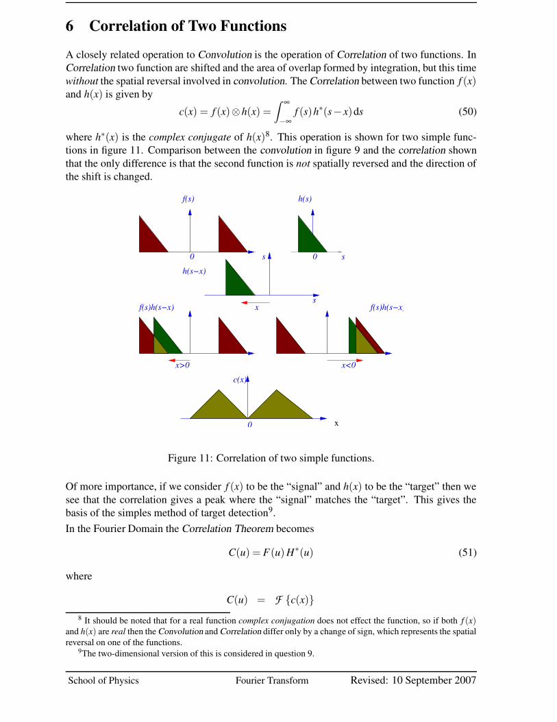
6 Correlation of Two FunctionsA closely related operation to Convolution is the operation of Correlation of two functions. InCorrelation two function are shifted and the area of overlap formed by integration, but this timewithout the spatial reversal involved in convolution. The Correlation between two function f (x)and h(x) is given by

c(x) = f (x)⊗h(x) =Z ∞

−∞f (s)h∗(s− x)ds (50)

where h∗(x) is the complex conjugate of h(x)8. This operation is shown for two simple func-tions in figure 11. Comparison between the convolution in figure 9 and the correlation shownthat the only difference is that the second function is not spatially reversed and the direction ofthe shift is changed.

x

f(s)h(s−x)

h(s)f(s)

h(s−x)

f(s)h(s−x)

x>0c(x)

0

sx

0

0 s

x<0

s

Figure 11: Correlation of two simple functions.

Of more importance, if we consider f (x) to be the “signal” and h(x) to be the “target” then wesee that the correlation gives a peak where the “signal” matches the “target”. This gives thebasis of the simples method of target detection9.In the Fourier Domain the Correlation Theorem becomes

C(u) = F(u) H∗(u) (51)

where

C(u) = F {c(x)}8 It should be noted that for a real function complex conjugation does not effect the function, so if both f (x)

and h(x) are real then the Convolution and Correlation differ only by a change of sign, which represents the spatialreversal on one of the functions.

9The two-dimensional version of this is considered in question 9.


-16 FOURIER BOOKLET

F(u) = F { f (x)}H(u) = F {h(x)}

It should be noted that the Fourier Transform H(u) is generally complex, and the complexconjugation is of vital significance to the operation.This is again a linear operation, which is distributative, but however is not commutative, sinceif

c(x) = f (x)⊗h(x)

then we can show thath(x)⊗ f (x) = c∗(−x)

In two dimensions we have the correlation between two functions given by

c(x,y) = f (x,y)⊗h(x,y) =Z Z

f (s, t)h∗(s− x, t − y)dsdt (52)

which in Fourier space gives,C(u,v) = F(u,v) H∗(u,v) (53)

Correlation is used in optics to to characterise the incoherent optical properties of a system andin digital imaging as a measure of the “similarity” between two images.

6.1 AutocorrelationIf we consider the special case of correlation with two identical real space functions, we obtainthe correlation of the input function with itself, being known as the Autocorrelation, being,

a(x,y) = f (x,y)⊗ f (x,y) (54)

so that in Fourier space we have,

A(u,v) = F(u,v) F∗(u,v) = |F(u,v)|2 (55)

which is the Power Spectrum of the function f (x,y). Therefore the Autocorrelation of a func-tion is given by the Inverse Fourier Transform of the Power Spectrum, giving,

a(x,y) = F −1{|F(u,v)|2}

(56)

In this case the correlation must be commutative, so we have that

a∗(−x,−y) = a(x,y)

If in addition the function f (x) is real, then clearly the correlation of a real function with it selfis real, so that a(x) is real. Therefore for a real function the autocorrelation is symmetric.


FOURIER BOOKLET -17

Workshop Questions

7 Questions

7.1 The sinc() function

State the expression for sinc(x) in terms of sin(x), and prove that

sinc(0) = 1

Sketch the graph ofy = sinc(ax) and y = sinc2(ax)

where a is a constant, and identify the locations of the zeros in each case.

Solution

The definition of sinc(x) is

sinc(x) =sin(x)

x

To find the value as x → 0 take the Taylor expansion about x = 0 to get,

sin(x) = x− x3

3! +x5

5! − . . .

so we have that

sinc(x) = 1− x2

3! +x4

5! − . . .

so, when x = 0 then sinc(0) = 1 as expected.Sketch of sinc(ax) when a = 4

-0.4

-0.2

0

0.2

0.4

0.6

0.8

1

-4 -2 0 2 4

sinc(4*x)

and sketch of sinc2(ax) when a = 4


-18 FOURIER BOOKLET

0

0.1

0.2

0.3

0.4

0.5

0.6

0.7

0.8

0.9

1

-4 -2 0 2 4

sinc(4*x)**2

Both functions have zero in the same place, when ax = ±nπ, so at

xn = ±nπa n = 1,2, . . .

Note the larger a the closer the zero are together.

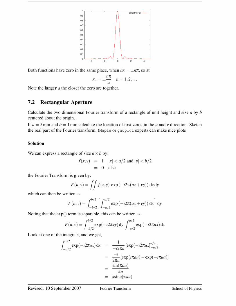
7.2 Rectangular ApertureCalculate the two dimensional Fourier transform of a rectangle of unit height and size a by bcentered about the origin.If a = 5mm and b = 1mm calculate the location of first zeros in the u and v direction. Sketchthe real part of the Fourier transform. (Maple or gnuplot experts can make nice plots)

Solution

We can express a rectangle of size a×b by:f (x,y) = 1 |x| < a/2 and |y| < b/2

= 0 elsethe Fourier Transform is given by:

F(u,v) =

Z Z

f (x,y) exp(−ı2π(ux+ vy)) dxdy

which can then be written as:

F(u,v) =Z b/2

−b/2

[

Z a/2

−a/2exp(−ı2π(ux+ vy)) dx

]

dy

Noting that the exp() term is separable, this can be written as

F(u,v) =Z b/2

−b/2exp(−ı2πvy)dy

Z a/2

−a/2exp(−ı2πux)dx

Look at one of the integrals, and we get,Z a/2

−a/2exp(−ı2πux)dx =

1−ı2πu [exp(−ı2πux]a/2

−a/2

=−ı

2πu [exp(ıπau)− exp(−ıπua)]

=sin(πau)

πu= asinc(πau)


FOURIER BOOKLET -19

The other integral is of exactly the same form, so that the Fourier transform of the rectangle is:

F(u,v) = absinc(πau)sinc(πbv)

The zero of this function occur at:

un = ±na for n = 1,2,3, . . .

vm = ±mb for m = 1,2,3, . . .

which if a = 5mm and b = 1mm then

un = 0.2mm−1,0.4mm−1,0.6mm−1, . . .

vn = 1mm−1,2mm−1,3mm−1, . . .

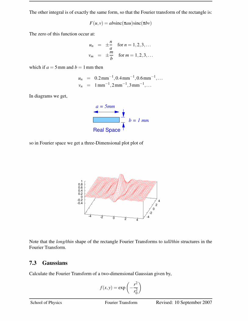
In diagrams we get,

a = 5mm

b = 1 mm

Real Space

so in Fourier space we get a three-Dimensional plot plot of

-4 -2 0 2 4-4

-2 0

2 4-0.4

-0.2 0

0.2 0.4 0.6 0.8

1

Note that the long/thin shape of the rectangle Fourier Transforms to tall/thin structures in theFourier Transform.

7.3 GaussiansCalculate the Fourier Transform of a two-dimensional Gaussian given by,

f (x,y) = exp(

−r2

r20

)


-20 FOURIER BOOKLET

where r2 = x2 + y2 and r0 is the radius of the e−1 point.You may use the standard mathematical identity that

Z ∞

−∞exp(−bx2) exp(iax)dx =

√

πb exp

(

−a2

4b

)

Solution

The Fourier Transform is given by:

F(u,v) =Z Z

exp(

−(x2 + y2)

r20

)

exp(−ı2π(ux+ vy))dxdy

Since the Gaussian and the Fourier kernel are separable, this can be written as

F(u,v) =Z

exp(

−x2

r20

)

exp(−ı2πux)dxZ

exp(

−y2

r20

)

exp(−ı2πvy)dy

so we need only evaluate one integral.Noting the result given that

Z ∞

−∞exp(−bx2)exp(iax)dx =

√

πb exp

(

−a2

4b

)

See “Mathematical Handbook”, M.R. Spiegel, McGraw-Hill, Page 98, Definite Integral 15.73.The given identity is actually,

Z ∞

0exp(−bx2)cos(ax)dx =

12

√

πb exp

(

−a2

4b

)

but this can be extended to the ∞ → ∞ exp() integral required by noting that the cos() is sym-metric so −∞ → ∞ integral is double the 0 → ∞ integral and that sin() is anti-symmetric so theimaginary part of the integral from ∞ → ∞ is zero.Then if be let b = 1/r2

0 and a = 2πu, thenZ

exp(

−x2

r20

)

exp(−ı2πux)dx =

√π

r0exp(

−π2r20u2)

which is also a Gaussian.Key Result: The Fourier Transform of a Gaussian is a Gaussian. It is the only function that isits own Fourier Transform.Exactly the same expression for the y integral, so we get that

F(u,v) =πr2

0exp(

−π2r20(u2 + v2)

)

which is more conveniently written as:

F(u,v) =πr2

0exp(

−w2

w20

)


FOURIER BOOKLET -21

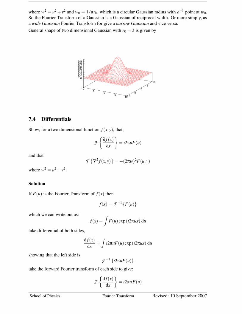
where w2 = u2 + v2 and w0 = 1/πr0, which is a circular Gaussian radius with e−1 point at w0.So the Fourier Transform of a Gaussian is a Gaussian of reciprocal width. Or more simply, asa wide Gaussian Fourier Transform for give a narrow Gaussian and vice versa.General shape of two dimensional Gaussian with r0 = 3 is given by

-10-5

0 5

10-10-5

0 5

10 0 0.1 0.2 0.3 0.4 0.5 0.6 0.7 0.8 0.9 1

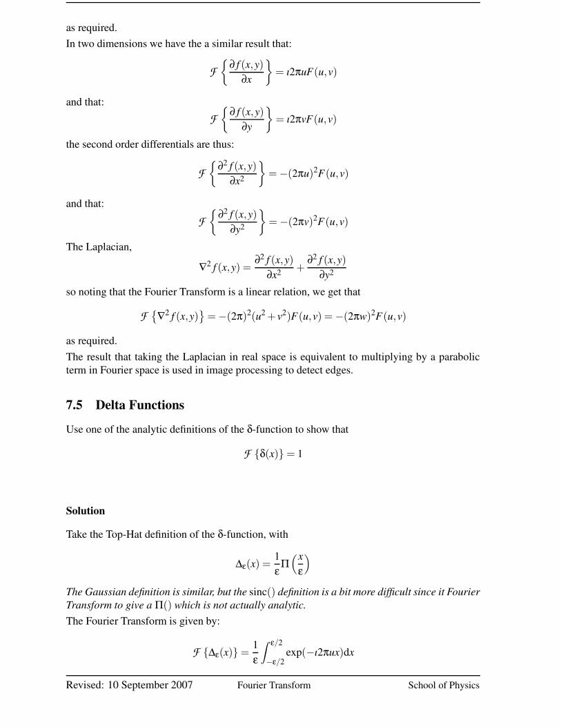
7.4 DifferentialsShow, for a two dimensional function f (x,y), that,

F{

∂ f (x)∂x

}

= ı2πuF(u)

and thatF {∇2 f (x,y)

}

= −(2πw)2F(u,v)

where w2 = u2 + v2.

Solution

If F(u) is the Fourier Transform of f (x) then

f (x) = F −1 {F(u)}

which we can write out as:f (x) =

Z

F(u)exp(ı2πux) du

take differential of both sides,

d f (x)dx =

Z

ı2πuF(u)exp(ı2πux) du

showing that the left side isF −1 {ı2πuF(u)}

take the forward Fourier transform of each side to give:

F{

d f (x)dx

}

= ı2πuF(u)


-22 FOURIER BOOKLET

as required.In two dimensions we have the a similar result that:

F{

∂ f (x,y)∂x

}

= ı2πuF(u,v)

and that:F{

∂ f (x,y)∂y

}

= ı2πvF(u,v)

the second order differentials are thus:

F{

∂2 f (x,y)∂x2

}

= −(2πu)2F(u,v)

and that:F{

∂2 f (x,y)∂y2

}

= −(2πv)2F(u,v)

The Laplacian,

∇2 f (x,y) =∂2 f (x,y)

∂x2 +∂2 f (x,y)

∂y2

so noting that the Fourier Transform is a linear relation, we get that

F {∇2 f (x,y)}

= −(2π)2(u2 + v2)F(u,v) = −(2πw)2F(u,v)

as required.The result that taking the Laplacian in real space is equivalent to multiplying by a parabolicterm in Fourier space is used in image processing to detect edges.

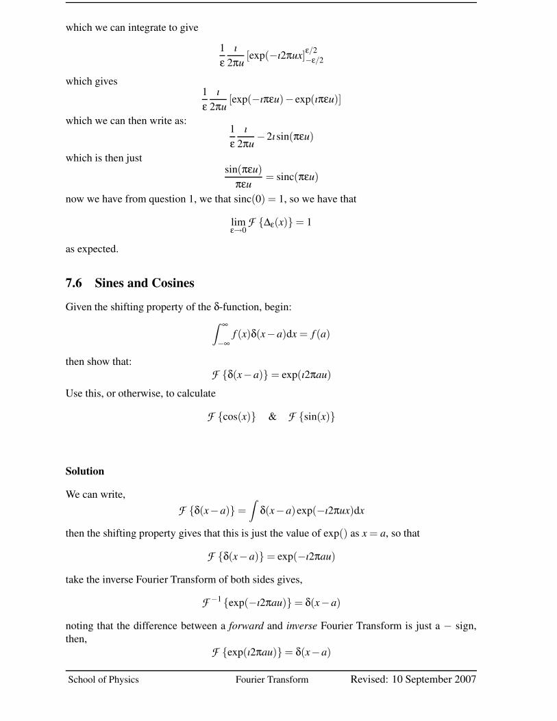
7.5 Delta FunctionsUse one of the analytic definitions of the δ-function to show that

F {δ(x)} = 1

Solution

Take the Top-Hat definition of the δ-function, with

∆ε(x) =1ε

Π(x

ε

)

The Gaussian definition is similar, but the sinc() definition is a bit more difficult since it FourierTransform to give a Π() which is not actually analytic.The Fourier Transform is given by:

F {∆ε(x)} =1ε

Z ε/2

−ε/2exp(−ı2πux)dx


FOURIER BOOKLET -23

which we can integrate to give

1ε

ı2πu [exp(−ı2πux]ε/2

−ε/2

which gives1ε

ı2πu [exp(−ıπεu)− exp(ıπεu)]

which we can then write as:1ε

ı2πu −2ısin(πεu)

which is then justsin(πεu)

πεu = sinc(πεu)

now we have from question 1, we that sinc(0) = 1, so we have that

limε→0

F {∆ε(x)} = 1

as expected.

7.6 Sines and CosinesGiven the shifting property of the δ-function, begin:

Z ∞

−∞f (x)δ(x−a)dx = f (a)

then show that:F {δ(x−a)} = exp(ı2πau)

Use this, or otherwise, to calculate

F {cos(x)} & F {sin(x)}

Solution

We can write,F {δ(x−a)} =

Z

δ(x−a)exp(−ı2πux)dx

then the shifting property gives that this is just the value of exp() as x = a, so that

F {δ(x−a)} = exp(−ı2πau)

take the inverse Fourier Transform of both sides gives,

F −1 {exp(−ı2πau)} = δ(x−a)

noting that the difference between a forward and inverse Fourier Transform is just a − sign,then,

F {exp(ı2πau)}= δ(x−a)


-24 FOURIER BOOKLET

let a = 1/2π and interchange x and u to give,

F {exp(ıx)} = δ(

u− 12π

)

Now, noting that the Fourier Transform is linear, then:

F {cos(x)} =12 [F {exp(ıx)}+F {exp(−ıx)}] = 1

2

[

δ(

u− 12π

)

+δ(

u+1

2π

)]

and similarly,

F {sin(x)} =12ı [F {exp(ıx)}−F {exp(−ıx)}] =

12ı

[

δ(

u− 12π

)

−δ(

u+1

2π

)]

so cos() and sin() Fourier transform to give a single frequency, as expected.

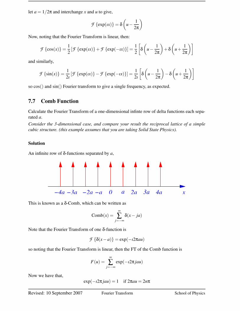
7.7 Comb FunctionCalculate the Fourier Transform of a one-dimensional infinte row of delta functions each sepa-rated a.Consider the 3-dimensional case, and compare your result the reciprocal lattice of a simplecubic structure. (this example assumes that you are taking Solid State Physics).

Solution

An infinite row of δ-functions separated by a,

−3a−4a x4a3a2aa0−a−2aThis is known as a δ-Comb, which can be written as

Comb(x) =∞

∑j=−∞

δ(x− ja)

Note that the Fourier Transform of one δ-function is

F {δ(x−a)} = exp(−ı2πau)

so noting that the Fourier Transform is linear, then the FT of the Comb function is

F(u) =∞

∑j=−∞

exp(−ı2π jau)

Now we have that,exp(−ı2π jau) = 1 if 2πau = 2nπ


FOURIER BOOKLET -25

so that thenu =

na ⇒ exp(−ı2π jau) = 1 ∀ j

to the Fourier Transform

F(u) → ∞ when u = n/a (In Phase)→ 0 when u 6= n/a (Out of Phase)

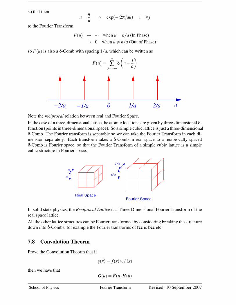
so F(u) is also a δ-Comb with spacing 1/a, which can be written as

F(u) =∞

∑j=−∞

δ(

u− ja

)

−1/a 0 1/a u2/a−2/aNote the reciprocal relation between real and Fourier Space.In the case of a three-dimensional lattice the atomic locations are given by three-dimensional δ-function (points in three-dimensional space). So a simple cubic lattice is just a three-dimensionalδ-Comb. The Fourier transform is separable so we can take the Fourier Transform in each di-mension separately. Each transform takes a δ-Comb in real space to a reciprocally spacedδ-Comb is Fourier space, so that the Fourier Transform of a simple cubic lattice is a simplecubic structure in Fourier space.

Real SpaceFourier Space

1/a

1/aa

a

In solid state physics, the Reciprocal Lattice is a Three-Dimensional Fourier Transform of thereal space lattice.All the other lattice structures can be Fourier transformed by considering breaking the structuredown into δ-Combs, for example the Fourier transforms of fcc is bcc etc.

7.8 Convolution TheormProve the Convolution Theorm that if

g(x) = f (x)�h(x)

then we have thatG(u) = F(u)H(u)


-26 FOURIER BOOKLET

where F(u) = F { f (x)} etc.The Convolution is frequently described as Fold-Shift-Multiply-Add. Explain this be means ofsketch diagrams in one-dimension.

Solution

Convolution is defined as

g(x) = f (x)�h(x) =Z ∞

−∞f (s)h(x− s)ds

Now take the Fourier Transform of both sides, to getZ

g(x)exp(−ı2πux)dx =

Z

[

Z ∞

−∞f (s)h(x− s)ds

]

exp(−ı2πux)dx

The Fourier Transform is linear, so the order of integration does not matter, so we get

G(u) =

Z Z

f (s)h(x− s)exp(−ı2πux)dsdx

Now let t = x− s so we get

G(u) =Z Z

f (s)h(t)exp(−ı2πu(s+ t))dsdt

=Z

f (s)exp(−ı2πus)dsZ

h(t)exp(−ı2πut)dt

= F(u)H(u)

where F(u) = F { f (x)}, H(u) = F {h(x)} and G(u) = F {g(x)}.Convolution can be described as:

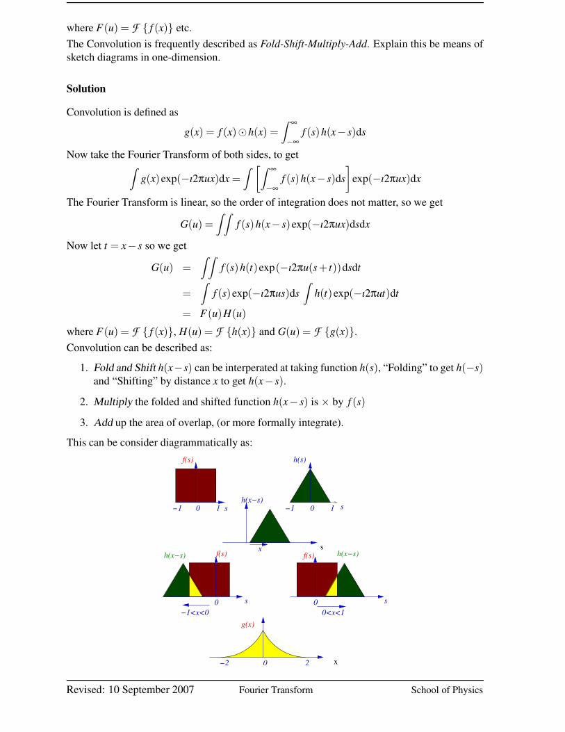
1. Fold and Shift h(x−s) can be interperated at taking function h(s), “Folding” to get h(−s)and “Shifting” by distance x to get h(x− s).

2. Multiply the folded and shifted function h(x− s) is × by f (s)

3. Add up the area of overlap, (or more formally integrate).

This can be consider diagrammatically as:

x

s

h(s)

h(x−s)

f(s)

f(s) h(x−s)h(x−s) f(s)

0<x<10 s

−1<x<00 s

−1 1 s0 −1 0 1 s

x

−2 0 2

g(x)


FOURIER BOOKLET -27

7.9 Correlation TheormProve the Correlation Theorm that if

c(x) = f (x)⊗h(x)

thenC(u) = F(u)H∗(u)

and also thath(x)⊗ f (x) = c∗(−x)

Show how the Correlation of two images is sometimes called “template-matching”.

Solution

Correlation is defined as

c(x) = f (x)⊗h(x) =

Z ∞

−∞f (s)h∗(s− x)ds

Now take the Fourier Transform of both sides, to getZ

c(x)exp(−ı2πux)dx =Z

[

Z ∞


]

exp(−ı2πux)dx

The Fourier Transform is linear, so the order of integration does not matter, so we get

C(u) =

Z Z

f (s)h∗(s− x)exp(−ı2πux)dsdx

Now let t = s− x so we get

C(u) =Z Z

f (s)h∗(t)exp(−ı2πu(s− t))dsdt

=

Z

f (s)exp(−ı2πus)dsZ

h(t)∗ exp(ı2πut)dt

=

Z

f (s)exp(−ı2πus)ds[

Z

h(t)exp(−ı2πut)dt]∗

= F(u)H∗(u)

where F(u) = F { f (x)}, H(u) = F {h(x)} and C(u) = F {c(x)}.Correlation is very similar to convolution except the second function is not folded and thedirection of the shift is reversed. We have that,

c(x) =

Z ∞


so taking the complex conjugate, we have that

c∗(x) =

Z ∞

−∞f ∗(s)h(s− x)ds

Now let t = s− x, so wec∗(x) =

Z ∞

−∞f ∗(t + x)h(t)dt


-28 FOURIER BOOKLET

then letting y = −x, we getc∗(−y) =

Z ∞

−∞h(t) f ∗(t − y)dt

so that we have thath(x)⊗ f (x) = c∗(−x)

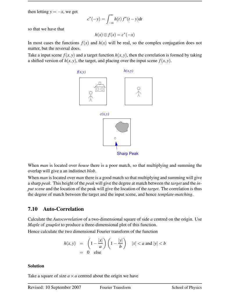
In most cases the functions f (x) and h(x) will be real, so the complex conjugation does notmatter, but the reversal does.Take a input scene f (x,y) and a target function h(x,y), then the correlation is formed by takinga shifted version of h(x,y), the target, and placing over the input scene f (x,y).

Sharp Peak

f(x,y) h(x,y)

c(x,y)

When man is located over house there is a poor match, so that multiplying and summing theoverlap will give a an indistinct blob.When man is located over man there is a good match so that multiplying and summing will givea sharp peak. This height of the peak will give the degree at match between the target and the in-put scene and the location of the peak will give the location of the target. The correlation is thusthe degree of match between the target and the input scene, and hence template-matching.

7.10 Auto-CorrelationCalculate the Autocorrelation of a two-dimensional square of side a centred on the origin. UseMaple of gnuplot to produce a three-dimensional plot of this function.Hence calculate the two dimensional Fourier transform of the function

h(x,y) =

(

1− |x|a

)(

1− |y|b

)

|x| < a and |y| < b

= 0 else

Solution

Take a square of size a×a centred about the origin we have


FOURIER BOOKLET -29

a/2

x

−a/2

y

a

a

a/2−a/2

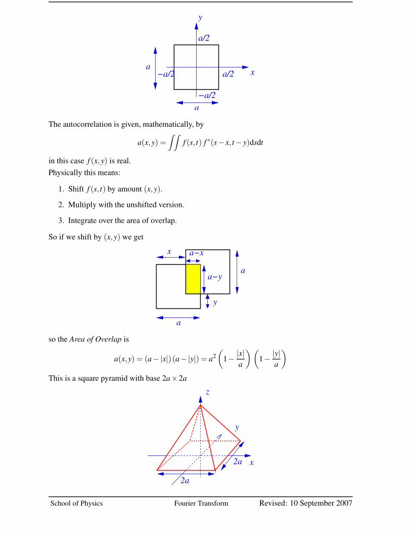
The autocorrelation is given, mathematically, by

a(x,y) =

Z Z

f (s, t) f ∗(s− x, t − y)dsdt

in this case f (x,y) is real.Physically this means:

1. Shift f (s, t) by amount (x,y).

2. Multiply with the unshifted version.

3. Integrate over the area of overlap.

So if we shift by (x,y) we get

x

a

a−y

y

a

a−x

so the Area of Overlap is

a(x,y) = (a−|x|)(a−|y|) = a2(

1− |x|a

) (

1− |y|a

)

This is a square pyramid with base 2a×2az

2a

2a

y

x


-30 FOURIER BOOKLET

Note that the autocorrelation is twice the size of of the original square.The function h(x,y) is the Normalised Autocorrelation, so that

h(x,y) =a(x,y)

a2

The Fourier Transform of h(x,y) is

H(u,v) = F {h(x,y)} =1a2 F {a(x,y)} =

1a2 A(u,v)

The autocorrelation theorem gives at

a(x,y) = f (x,y)⊗ f (x,y)A(u,v) = |F(u,v)|2

Now f (x,y) is a square of size a×a, so from Question 2 we have that.

F(u,v) = a2sinc(πau)sinc(πav)

So we have thatA(u,v) = a4sinc2(πau)sinc2(πav)

and so the required Fourier Transform

H(u,v) = a2sinc2(πau)sinc2(πav)

This is much easier than trying to form the direct Fourier Transform.


Documents

The Fourier Transform (What you need to know)wjh/teaching/Fourier/documents/booklet.pdf · The Fourier Transform (What you need to know) ... This slightly odd convention and is to