The geometry of incompatibility in growing soft tissues

J. Mech. Phys. Solids 146 (2021) 104177

A0

TnTAa

b

c

d

e

A

KFGBSR

1

ivss

hR

Contents lists available at ScienceDirect

Journal of the Mechanics and Physics of Solids

journal homepage: www.elsevier.com/locate/jmps

he geometry of incompatibility in growing soft tissues: Theory andumerical characterizationaeksang Lee a,∗, Maria A. Holland b, Johannes Weickenmeier c, Arun K. Gosain d,drian Buganza Tepole a,e

School of Mechanical Engineering, Purdue University, West Lafayette, IN, USAAerospace & Mechanical Engineering, University of Notre Dame, Notre Dame, IN, USADepartment of Mechanical Engineering, Stevens Institute of Technology, Hoboken, NJ, USALurie Children Hospital, Northwestern University, Chicago, IL, USAWeldon School of Biomedical Engineering, Purdue University, West Lafayette, IN, USA

R T I C L E I N F O

eywords:inite plasticityrowth and remodelingrain mechanicskin mechanicsesidual stress

A B S T R A C T

Tissues in vivo are not stress-free. As we grow, our tissues adapt to different physiological anddisease conditions through growth and remodeling. This adaptation occurs at the microscopicscale, where cells control the microstructure of their immediate extracellular environment toachieve homeostasis. The local and heterogeneous nature of this process is the source of residualstresses. At the macroscopic scale, growth and remodeling can be accurately captured with thefinite volume growth framework within continuum mechanics, which is akin to plasticity. Themultiplicative split of the deformation gradient into growth and elastic contributions bringsabout the notion of incompatibility as a plausible description for the origin of residual stress.Here we define the geometric features that characterize incompatibility in biological materials.We introduce the geometric incompatibility tensor for different growth types, showing that theconstraints associated with growth lead to specific patterns of the incompatibility metrics. Tonumerically investigate the distribution of incompatibility measures, we implement the analysiswithin a finite element framework. Simple, illustrative examples are shown first to explainthe main concepts. Then, numerical characterization of incompatibility and residual stress isperformed on three biomedical applications: brain atrophy, skin expansion, and cortical folding.Our analysis provides new insights into the role of growth in the development of tissue defectsand residual stresses. Thus, we anticipate that our work will further motivate additional researchto characterize residual stresses in living tissue and their role in development, disease, andclinical intervention.

. Introduction

It is well known that soft tissues in their physiological environment are not stress-free (Vaishnav and Vossoughi, 1987). Fornstance, skin has been shown to have pre-strain in vivo (Tepole et al., 2015). This is also observed in the heart and heartalves (Rausch and Kuhl, 2013; Omens et al., 2003). It has been hypothesized that the state of pre-stress of different organs yieldspecific physiological function (Fung, 1995). For example, residual stresses in arteries actually reduce the peak stresses duringystole (Vaishnav and Vossoughi, 1987). Experimentally, the opening angle experiment of arteries was the first method introduced

∗ Corresponding author.

vailable online 17 October 2020022-5096/© 2020 Elsevier Ltd. All rights reserved.

E-mail addresses: [email protected], [email protected] (T. Lee).

ttps://doi.org/10.1016/j.jmps.2020.104177eceived 23 May 2020; Received in revised form 4 September 2020; Accepted 3 October 2020

http://www.elsevier.com/locate/jmps

http://www.elsevier.com/locate/jmps

mailto:[email protected]

mailto:[email protected]

https://doi.org/10.1016/j.jmps.2020.104177

http://crossmark.crossref.org/dialog/?doi=10.1016/j.jmps.2020.104177&domain=pdf

https://doi.org/10.1016/j.jmps.2020.104177

Journal of the Mechanics and Physics of Solids 146 (2021) 104177T. Lee et al.

hI2eaitrs

DhgweaBp

ppdEgsidtq

gudotaaeamuscmg

votgwcobahul

to measure residual deformation (Chuong and Fung, 1986). Thick slices of whole hearts have been dissected and then cut to measurethe opening angle of these slices and, by extension, the residual stress of the heart (Omens and Fung, 1990; Genet et al., 2015).Heart valves have been measured in vivo and ex vivo to quantify their overall pre-strain (Rausch et al., 2011a). Such approacheshave further cemented the existence of pre-strain in vivo, but they are incomplete because they reduce the residual strain field to aomogeneous indicator like the scalar opening angle. The true state of residual deformation is more complex (Fung and Liu, 1989).ndeed, there is evidence that tissues develop heterogeneous patterns of residual deformation during growth (Taber and Humphrey,001). In response to skin expansion, for instance, the residual deformation of skin varies across the entire expanded region (Tepolet al., 2016). Even restricting the attention to the opening angle measurement, significant variation of this pre-strain metric varieslong the length of an artery (Fung, 2013). Thus, although numerous previous studies have confirmed the existence of pre-strainn living tissue, the precise features of this field are still poorly understood. Increasing our understanding of the basic mechanismshat can drive the development of residual strain in soft tissues has significant implications: it would allow estimation of the trueeference configuration, the true mechanical behavior of tissues with respect to a stress-free state, and the way in which residualtrain contributes to the tissue mechanical function in vivo (Lanir, 2009; Rausch et al., 2017).

Residual stresses are not just a feature that emerges from tissue growth and remodeling. The opposite question is equally relevant:oes residual strain and stress guide the growth and remodeling process itself, and if so, how? Advances in mechanobiology haveelped elucidate the way in which cells can sense mechanical cues. Yet, it is not clear how these cues can be coordinated duringrowth and remodeling to achieve a desired homeostatic state that is not stress-free (Humphrey et al., 2014). Work on Drosophilaing disc development has brought up residual stress as a key regulator to explain embryo development patterns that are notxplained by morphogen gradients alone (Nienhaus et al., 2009; Schluck et al., 2013). In Ciarletta et al. (2016), the authors proposeformulation of tissue growth and remodeling by considering a residual stress field directly as a target for tissue homeostasis.

eyond animal tissues, work in plant development has also characterized mismatch in growth rates between adjacent regions of thelant as a source of tissue conflicts that guide plant morphogenesis (Echevin et al., 2019; Rebocho et al., 2017).

Among different theoretical frameworks of growth and remodeling, a phenomenological description adopted from the theory oflasticity has been particularly successful (Lubarda, 2004; Ambrosi et al., 2011; Eskandari and Kuhl, 2015). In finite deformationlasticity, the deformation gradient is multiplicatively split into elastic and inelastic deformations (Lee, 1969). Instead of a plasticeformation, the corresponding tensor in biomechanics is termed the growth deformation tensor (Rodriguez et al., 1994; Taber andggers, 1996), and captures addition of mass by changes in volume (Himpel et al., 2005). The decomposition of the deformationradient tensor plays a key role in understanding the origin of residual stresses observed at the macroscopic scale. The multiplicativeplit in fact introduces a geometric origin for the residual stress (Lubliner, 2008). Growth and elastic deformations are in generalncompatible fields, which means that they cannot be obtained from a displacement field (Skalak et al., 1996). If the growtheformation is incompatible, an incompatible elastic deformation is required to ensure compatibility of the total deformation. Inurn, the necessary incompatibility of the elastic deformation is the source of the residual stress field (Steinmann, 2015). Thus,uantifying the incompatibility of growth fields is intimately linked to the understanding of residual strains.

The notion of incompatibility arising from the multiplicative split of the deformation gradient is common between plasticity androwth, but the physical mechanisms leading to incompatibility and residual stresses are different between the two. In crystals, it isniversally acknowledged that plastic deformation occurs through the movement of a dislocation, which is the most important lineefect in crystals (Lubliner, 2008). Mismatch in the deformation between adjacent regions in the crystal results in the disruptionf the lattice structure (Withers and Bhadeshia, 2001; De Wit, 1981). The defect in the lattice at the atomic scale is captured athe macroscopic scale via the plastic deformation tensor. Defects or imperfections of the lattice accommodated by the dislocationre connected to the storage of additional energy and, hence, residual stress (Hirth et al., 1983; Hurtado and Ortiz, 2013; Menzelnd Steinmann, 2000). Other types of topological defects in crystals can lead to residual stresses, for instance quasi-plastic thermalxpansion (De Wit, 1981; Clayton et al., 2005; Miri and Rivier, 2002). In soft tissues, on the other hand, the physical mechanismt the microscale behind the accumulation of residual stress is still unclear (Lanir, 2009). Hypotheses include: differences inechanical properties between adjacent structures within the tissue (Taber and Humphrey, 2001), different growth rates leading tonequal material accumulation (Vandiver and Goriely, 2009), microstructure reorganization (Taber and Eggers, 1996; Fung, 2013),urface accretion (Tomassetti et al., 2016; Abi-Akl and Cohen, 2020), and multiple and evolving natural configurations for differentonstituents (Humphrey and Rajagopal, 2002). Even if the precise microscopic origin of the residual stress is still in question, theacroscopic observation captured by the framework of finite volume growth condenses the origin of the residual stress field to

eometric mismatches in the soft tissue stress-free configuration due to a heterogeneous growth and remodeling field.In this manuscript, we quantify the geometric incompatibility that arises during growth of soft tissue described by the finite

olume growth framework. This geometric characterization is linked to the origin of residual stress at the continuum scale. Forur analysis, we rely on some well-established tools from crystal physics, such as the re-interpretation of the Burgers vector andhe geometric dislocation density tensor (Kröner, 1959; Cermelli and Gurtin, 2001). In plasticity, the Burgers vector explains theeometry of the dislocation density (Kondo, 1952, 1955; Nye, 1953). Soft tissues do not accumulate dislocations due to growth, bute can still use similar geometric analysis to understand the type of incompatibility possible in growing tissue, and how it may be

onnected to the accumulation of residual stress. We derive the form of the local Burgers vector density for representative scenariosf volumetric, area, and fiber growth. Moreover, we also characterize incompatibility and the associated residual stress for relevantiomedical applications such as human brain atrophy and skin expansion. We believe that our results will provide new insightsnd foster discussion about the geometric incompatibility induced by growth, how it may be related to microscale phenomena, andow it is connected to the accumulation of residual stress. Moreover, we anticipate that this work will not only improve our basicnderstanding of tissue mechanics, but also be useful for medical interventions that trigger growth and remodeling of soft tissues

2

eading to accumulation of residual stress that can impact tissue function.


𝐱ggt

waT

wo

tc𝐅ots

wut

sncida

2

aCahd

2. Materials and methods

2.1. Kinematics of growth

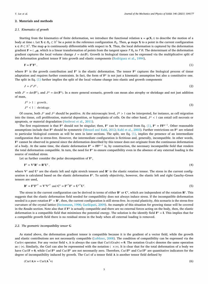
Starting from the kinematics of finite deformation, we introduce the functional relation 𝐱 = 𝝋(𝐗, 𝑡) to describe the motion of abody at time 𝑡. Let 𝐗 ∈ 0 ⊂ R3 be a point in the reference configuration 0. Then, 𝝋 maps 𝐗 to a point in the current configuration∈ ⊂ R3. The map 𝝋 is continuously differentiable with respect to 𝐗. Thus, the local deformation is captured by the deformationradient 𝐅 = ∇0𝝋, which is a linear transformation of points from the tangent space 0 to . The determinant of the deformationradient captures the local volume change 𝐽 = det(𝐅). Growth in biological tissues can be expressed via the multiplicative split ofhe deformation gradient tensor 𝐅 into growth and elastic components (Rodriguez et al., 1994),

𝐅 = 𝐅𝑒𝐅𝑔 , (1)

here 𝐅𝑔 is the growth contribution and 𝐅𝑒 is the elastic deformation. The tensor 𝐅𝑔 captures the biological process of tissuedaptation and requires further constraints. In fact, the form of 𝐅𝑔 is not just a kinematic assumption but also a constitutive one.he split in Eq. (1) further implies the split of the local volume change into elastic and growth components

𝐽 = 𝐽 𝑒𝐽 𝑔 , (2)

ith 𝐽 𝑒 = det(𝐅𝑒), and 𝐽 𝑔 = det(𝐅𝑔). In a more general scenario, growth can mean also atrophy or shrinkage and not just additionf mass,

𝐽 𝑔 > 1 ∶ growth ,

𝐽 𝑔 < 1 ∶ shrinkage .(3)

Of course, both 𝐽 𝑒 and 𝐽 𝑔 should be positive. At the microscopic level, 𝐽 𝑔 > 1 can be interpreted, for instance, as cell migrationinto the tissue, cell proliferation, material deposition, or hyperplasia of cells. On the other hand, 𝐽 𝑔 < 1 can entail cell necrosis orapoptosis, or material degradation (Ambrosi et al., 2011).

The first requirement is that 𝐅𝑔 should not be singular; then, 𝐅𝑒 can be recovered from Eq. (1), 𝐅𝑒 = 𝐅𝐅𝑔−1. Other reasonableassumptions include that 𝐅𝑔 should be symmetric (Menzel and Kuhl, 2012; Kuhl et al., 2003). Further restrictions on 𝐅𝑔 are relatedo particular biological contexts as will be seen in later sections. The split, see Eq. (1), implies the presence of an intermediateonfiguration that is stress-free. However, the intermediate configuration is fictitious and, generally, incompatible. In other words,𝑔 cannot be observed in general since the deformation described by this tensor does not originate from the continuous deformationf a body. At the same time, the elastic deformation 𝐅𝑒 = 𝐅𝐅𝑔−1 is, by construction, the necessary incompatible field that rendershe total deformation compatible. In turn, the need for 𝐅𝑒 to ensure compatibility even in the absence of any external loading is theource of residual stress.

Let us further consider the polar decomposition of 𝐅𝑒,

𝐅𝑒 = 𝐕𝑒𝐑𝑒 = 𝐑𝑒𝐔𝑒 , (4)

here 𝐕𝑒 and 𝐔𝑒 are the elastic left and right stretch tensors and 𝐑𝑒 is the elastic rotation tensor. The stress in the current config-ration is calculated based on the elastic deformation 𝐅𝑒. To satisfy objectivity, however, the elastic left and right Cauchy–Greenensors are used,

𝐁𝑒 = 𝐅𝑒𝐅𝑒⊤ = 𝐕𝑒𝐕𝑒⊤ and 𝐂𝑒 = 𝐅𝑒⊤𝐅𝑒 = 𝐔𝑒⊤𝐔𝑒. (5)

The stress in the current configuration can be derived in terms of either 𝐁𝑒 or 𝐂𝑒, which are independent of the rotation 𝐑𝑒. Thisuggests that the elastic deformation field needed for compatibility does not always induce stress. If the incompatible deformationeeded is a pure rotation 𝐅𝑒 = 𝐑𝑒, then, the current configuration is still stress-free. In crystal plasticity, this scenario is the stress-freeurvature of the crystal lattice (Steinmann, 1996; Garikipati, 2009). An example of this situation for growing tissue will be coveredn the Results section. Note also that if 𝐅𝑔 is actually compatible and there are no external forces acting on the body, then, the elasticeformation is a compatible field that minimizes the potential energy. The solution is the identify field 𝐅𝑒 = 𝐈. This implies that forcompatible growth field there is no residual stress in the body when all external loading is removed.

.2. The geometric incompatibility tensor 𝐆

As stated above, the deformation gradient tensor is compatible because it is the gradient of a vector field, while the growthnd elastic contributions are not necessarily compatible (Lubliner, 2008). The condition of compatibility can be expressed via theurl(∙) operator. For any vector field 𝐯, it is always the case that Curl (Grad𝐯) = 𝟎. The notation Grad(∙) denotes the same operations ∇(∙). Similarly, the Curl can also be represented with the notation ∇ × (∙). It is clear that for the total deformation of a body weave Curl𝐅 = 𝟎, while Curl𝐅𝑔 and Curl𝐅𝑒 are not necessarily zero. Therefore, Curl𝐅𝑔 and Curl𝐅𝑒 are quantitative indicators for theegree of incompatibility induced by growth. The Curl of a tensor field 𝐀 is another tensor field defined by

(Curl𝐀)𝐯 = Curl(𝐀⊤𝐯) (6)

3


ca

C

wiv2g

frgit

aUc

wdaa

for all constant vectors 𝐯. We use the notation Curl(∙) for the operation with respect to the reference configuration 𝐗, compared tourl(∙) which is with respect to the current configuration 𝐱 (Cermelli and Gurtin, 2001). In index notation, the components of Curl𝐀re

(Curl𝐀)𝑖𝑗 = 𝜀𝑖𝑟𝑠𝜕𝐴𝑗𝑠𝜕𝑋𝑟

, (7)

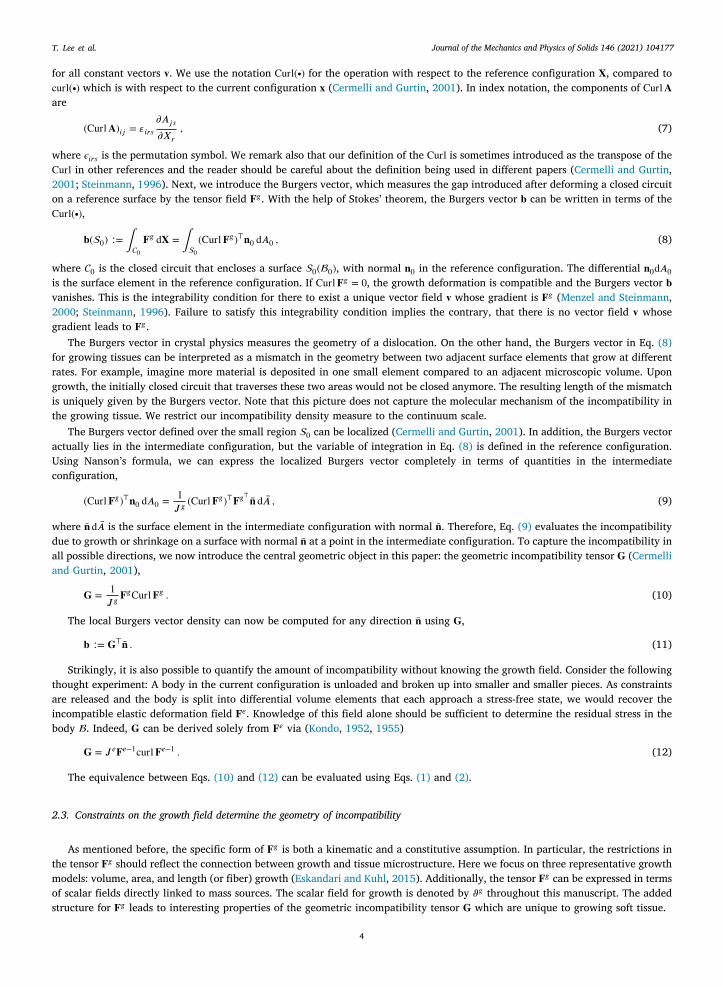
where 𝜖𝑖𝑟𝑠 is the permutation symbol. We remark also that our definition of the Curl is sometimes introduced as the transpose of theCurl in other references and the reader should be careful about the definition being used in different papers (Cermelli and Gurtin,2001; Steinmann, 1996). Next, we introduce the Burgers vector, which measures the gap introduced after deforming a closed circuiton a reference surface by the tensor field 𝐅𝑔 . With the help of Stokes’ theorem, the Burgers vector 𝐛 can be written in terms of theurl(∙),

𝐛(0) ∶= ∫0𝐅𝑔 d𝐗 = ∫0

(Curl𝐅𝑔)⊤𝐧0 d𝐴0 , (8)

here 0 is the closed circuit that encloses a surface 0(0), with normal 𝐧0 in the reference configuration. The differential 𝐧0d𝐴0s the surface element in the reference configuration. If Curl𝐅𝑔 = 0, the growth deformation is compatible and the Burgers vector 𝐛anishes. This is the integrability condition for there to exist a unique vector field 𝐯 whose gradient is 𝐅𝑔 (Menzel and Steinmann,000; Steinmann, 1996). Failure to satisfy this integrability condition implies the contrary, that there is no vector field 𝐯 whoseradient leads to 𝐅𝑔 .

The Burgers vector in crystal physics measures the geometry of a dislocation. On the other hand, the Burgers vector in Eq. (8)or growing tissues can be interpreted as a mismatch in the geometry between two adjacent surface elements that grow at differentates. For example, imagine more material is deposited in one small element compared to an adjacent microscopic volume. Uponrowth, the initially closed circuit that traverses these two areas would not be closed anymore. The resulting length of the mismatchs uniquely given by the Burgers vector. Note that this picture does not capture the molecular mechanism of the incompatibility inhe growing tissue. We restrict our incompatibility density measure to the continuum scale.

The Burgers vector defined over the small region 0 can be localized (Cermelli and Gurtin, 2001). In addition, the Burgers vectorctually lies in the intermediate configuration, but the variable of integration in Eq. (8) is defined in the reference configuration.sing Nanson’s formula, we can express the localized Burgers vector completely in terms of quantities in the intermediateonfiguration,

(Curl𝐅𝑔)⊤𝐧0 d𝐴0 =1𝐽 𝑔

(Curl𝐅𝑔)⊤𝐅𝑔⊤ �̄� d�̄� , (9)

here �̄� d�̄� is the surface element in the intermediate configuration with normal �̄�. Therefore, Eq. (9) evaluates the incompatibilityue to growth or shrinkage on a surface with normal �̄� at a point in the intermediate configuration. To capture the incompatibility inll possible directions, we now introduce the central geometric object in this paper: the geometric incompatibility tensor 𝐆 (Cermellind Gurtin, 2001),

𝐆 = 1𝐽 𝑔

𝐅𝑔Curl𝐅𝑔 . (10)

The local Burgers vector density can now be computed for any direction �̄� using 𝐆,

𝐛 ∶= 𝐆⊤�̄� . (11)

Strikingly, it is also possible to quantify the amount of incompatibility without knowing the growth field. Consider the followingthought experiment: A body in the current configuration is unloaded and broken up into smaller and smaller pieces. As constraintsare released and the body is split into differential volume elements that each approach a stress-free state, we would recover theincompatible elastic deformation field 𝐅𝑒. Knowledge of this field alone should be sufficient to determine the residual stress in thebody . Indeed, 𝐆 can be derived solely from 𝐅𝑒 via (Kondo, 1952, 1955)

𝐆 = 𝐽 𝑒𝐅𝑒−1curl𝐅𝑒−1 . (12)

The equivalence between Eqs. (10) and (12) can be evaluated using Eqs. (1) and (2).

2.3. Constraints on the growth field determine the geometry of incompatibility

As mentioned before, the specific form of 𝐅𝑔 is both a kinematic and a constitutive assumption. In particular, the restrictions inthe tensor 𝐅𝑔 should reflect the connection between growth and tissue microstructure. Here we focus on three representative growthmodels: volume, area, and length (or fiber) growth (Eskandari and Kuhl, 2015). Additionally, the tensor 𝐅𝑔 can be expressed in termsof scalar fields directly linked to mass sources. The scalar field for growth is denoted by 𝜗𝑔 throughout this manuscript. The added

𝑔

4

structure for 𝐅 leads to interesting properties of the geometric incompatibility tensor 𝐆 which are unique to growing soft tissue.


da

w

n

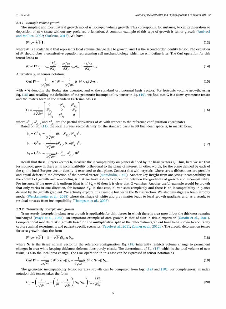
2.3.1. Isotropic volume growthThe simplest and most natural growth model is isotropic volume growth. This corresponds, for instance, to cell proliferation or

eposition of new tissue without any preferred orientation. A common example of this type of growth is tumor growth (Ambrosind Mollica, 2002; Ciarletta, 2013). We have

𝐅𝑔 ∶= 3√

𝜗𝑔𝐈 , (13)

where 𝜗𝑔 is a scalar field that represents local volume change due to growth, and 𝐈 is the second-order identity tensor. The evolutionof 𝜗𝑔 should obey a constitutive equation representing cell mechanobiology which we will define later. The Curl operation for thistensor leads to

(Curl𝐅𝑔)𝑖𝑗 = 𝜖𝑖𝑟𝑠𝜕𝐹 𝑔𝑗𝑠𝜕𝑋𝑟

=𝜕 3√

𝜗𝑔

𝜕𝑋𝑟𝜖𝑖𝑟𝑠𝛿𝑗𝑠 =

𝜕 3√

𝜗𝑔

𝜕𝑋𝑟𝜖𝑖𝑟𝑗 . (14)

Alternatively, in tensor notation,

Curl𝐅𝑔 = 1

3 3√

𝜗𝑔2⋆ ∇𝜗𝑔 = 1

3 3√

𝜗𝑔2(∇𝜗𝑔 × 𝐞𝑖)⊗ 𝐞𝑖 , (15)

with ⋆(∙) denoting the Hodge star operator, and 𝐞𝑖 the standard orthonormal basis vectors. For isotropic volume growth, usingEq. (15) and recalling the definition of the geometric incompatibility tensor in Eq. (10), we find that 𝐆 is a skew-symmetric tensorand the matrix form in the standard Cartesian basis is

𝐆 = 1

3 3√

𝜗𝑔4

⎡

⎢

⎢

⎢

⎣

0 −𝜗𝑔,𝑋3𝜗𝑔,𝑋2

𝜗𝑔,𝑋30 −𝜗𝑔,𝑋1

−𝜗𝑔,𝑋2𝜗𝑔,𝑋1

0

⎤

⎥

⎥

⎥

⎦

, (16)

here 𝜗𝑔,𝑋1, 𝜗𝑔,𝑋2

, and 𝜗𝑔,𝑋3are the partial derivatives of 𝜗𝑔 with respect to the reference configuration coordinates.

Based on Eq. (11), the local Burgers vector density for the standard basis in 3D Euclidean space is, in matrix form,

𝐛1 = 𝐆⊤𝐞1 =1

3 3√

𝜗𝑔4(0, −𝜗𝑔,𝑋3

, 𝜗𝑔,𝑋2)⊤ ,

𝐛2 = 𝐆⊤𝐞2 =1

3 3√

𝜗𝑔4(𝜗𝑔,𝑋3

, 0, −𝜗𝑔,𝑋1)⊤ ,

𝐛3 = 𝐆⊤𝐞3 =1

3 3√

𝜗𝑔4(−𝜗𝑔,𝑋2

, 𝜗𝑔,𝑋1, 0)⊤ .

(17)

Recall that these Burgers vectors 𝐛𝑖 measure the incompatibility on planes defined by the basis vectors 𝐞𝑖. Thus, here we see thatfor isotropic growth there is no incompatibility orthogonal to the plane of interest. In other words, for the plane defined by each ofthe 𝐞𝑖, the local Burgers vector density is restricted to that plane. Contrast this with crystals, where screw dislocations are possibleand entail defects in the direction of the normal vector (Maradudin, 1959). Another key insight from analyzing incompatibility inthe context of growth and remodeling is that we have a direct connection between the gradients of growth and incompatibility.For instance, if the growth is uniform (that is, if 𝜗𝑔,𝐗 = 0) then it is clear that 𝐆 vanishes. Another useful example would be growththat only varies in one direction, for instance 𝑋1. In that case, 𝐛1 vanishes completely and there is no incompatibility in planesdefined by the growth gradient. We actually explore this example further in the Results section. We also investigate a brain atrophymodel (Weickenmeier et al., 2018) where shrinkage of white and gray matter leads to local growth gradients and, as a result, toresidual stresses from incompatibility (Thompson et al., 2003).

2.3.2. Transversely isotropic area growthTransversely isotropic in-plane area growth is applicable for thin tissues in which there is area growth but the thickness remains

unchanged (Pasyk et al., 1988). An important example of area growth is that of skin in tissue expansion (Gosain et al., 2001).Computational models of skin growth based on the multiplicative split of the deformation gradient have been shown to accuratelycapture animal experiments and patient-specific scenarios (Tepole et al., 2011; Zöllner et al., 2012b). The growth deformation tensorfor area growth takes the form

𝐅𝑔 ∶=√

𝜗𝑔𝐈 + (1 −√

𝜗𝑔)𝐍0 ⊗ 𝐍0 , (18)

where 𝐍0 is the tissue normal vector in the reference configuration. Eq. (18) inherently restricts volume change to permanentchanges in area while keeping thickness deformations purely elastic. The determinant of Eq. (18), which is the total volume of newtissue, is also the local area change. The Curl operation in this case can be expressed in tensor notation as

Curl𝐅𝑔 = 1

2√

𝜗𝑔(∇𝜗𝑔 × 𝐞𝑖)⊗ 𝐞𝑖 −

1

2√

𝜗𝑔(∇𝜗𝑔 × 𝐍0)⊗ 𝐍0 . (19)

The geometric incompatibility tensor for area growth can be computed from Eqs. (19) and (10). For completeness, in indexotation this tensor takes the form

𝐺𝑖𝑗 =

(

1√

𝛿𝑖𝑚 +

(

1𝑔 − 1

√

)

𝑁0𝑖𝑁0𝑚

)

𝜖𝑚𝑟𝑠𝜕𝐹 𝑔𝑗𝑠 . (20)

5

𝜗𝑔 𝜗 𝜗𝑔 𝜕𝑋𝑟


H

ti

2

a1gw

wgo

i

Similar to the isotropic case, incompatibility occurs due to gradients in the permanent area change, as is evident from Eq. (19).aving an expression for 𝐆, we can determine the Burgers vector density in any direction. To that end, the most relevant plane

is defined by 𝐍0 or, more rigorously, the normal �̄� in the intermediate configuration. For this particular type of growth we have�̄� = 𝐍0 by construction. The local Burgers vector density 𝐆⊤�̄� becomes

𝐛 = 𝐆⊤�̄� = 1

2√

𝜗𝑔3(𝐬𝛼 ⊗ (∇𝜗𝑔 × 𝐬𝛼))�̄� , (21)

where the vectors 𝐬𝛼 , with 𝛼 = {1, 2}, are the local basis for the surface defined by �̄�. We observe again that the Burgers vectorcorresponding to the plane defined by �̄� is restricted to that plane and will have only components along the 𝐬𝛼 directions. Moreover,if the gradient is aligned with any of the surface basis vectors, then the expression can be further simplified. For instance, withoutloss of generality, assume that ∇𝜗𝑔 is aligned with 𝐬2 and denote 𝐬1 = 𝐬. The vector 𝐬 is the vector on the surface which is orthogonalto the in plane growth gradient. Then,

𝐛 =|∇𝜗𝑔|

2√

𝜗𝑔3𝐬 . (22)

This last expression condenses the key type of incompatibility of area growth. Since the local basis can always be aligned withhe direction of the growth gradient, Eq. (22) shows that the incompatibility is orthogonal to the growth gradient and its magnitudes proportional to the magnitude of the growth gradient scaled with respect to the amount of growth.

.3.3. Uniaxial fiber growthIn tissues such as muscle, growth can occur along the fiber direction (Wisdom et al., 2015; Zöllner et al., 2012a). In addition,

xons in the white matter of the brain also show lengthwise growth induced by chronic overstretch during development (Bray,984). Cortical folding of the brain is a phenomenon that occurs in part due to mechanical instabilities triggered by this type ofrowth coupled to other biological factors (Holland et al., 2015). The heart also has a unique and well-defined fiber structure alonghich growth can occur, especially due to volume overload. For growth along the fiber direction, 𝐅𝑔 is defined as

𝐅𝑔 ∶= 𝐈 + (𝜗𝑔 − 1)𝐟0 ⊗ 𝐟0 , (23)

here 𝐟0 is the fiber direction in the reference configuration. The determinant of Eq. (23) is the volume change, which in the fiberrowth scenario is also the irreversible change in length along the fiber direction. For this specific type of growth tensor, the Curlperator leads to an elegant form

Curl𝐅𝑔 = (∇𝜗𝑔 × 𝐟0)⊗ 𝐟0. (24)

The incompatibility tensor can then be computed based on its definition 𝐆 = (1∕𝜗𝑔)𝐅𝑔Curl𝐅𝑔 . For completeness, we write it inndex notation,

𝐺𝑖𝑗 =( 1𝜗𝑔𝛿𝑖𝑚 + (1 − 1

𝜗𝑔)𝑓0𝑖𝑓0𝑚

)

𝜖𝑚𝑟𝑠𝜕𝜗𝑔

𝜕𝑋𝑟𝑓0𝑗𝑓0𝑠 . (25)

For fiber growth, the fiber direction is unchanged in the intermediate configuration, 𝐟 = 𝐟0. The local Burgers vector density inthe plane defined by the fiber direction 𝐟 is

𝐆⊤𝐟 = 1𝜗𝑔

𝐟0 ⊗ (∇𝜗𝑔 × 𝐟0)𝐟 = 𝟎 . (26)

Thus, in the case of fiber growth, there cannot be incompatibility in the direction of the fiber. Also from Eq. (24), it can be seenthat if the gradient of growth is aligned with the direction of the fiber there is also no incompatibility. We turn our attention to theplanes orthogonal to the fiber direction. Consider the unit vector in the intermediate configuration �̄�, which is locally orthogonalto both the growth gradient and the fiber direction. Then, the local Burgers vector density for the plane defined by �̄� is

𝐆⊤�̄� =|∇𝜗𝑔| sin(𝛽)

𝜗𝑔𝐟0 , (27)

where 𝛽 is the angle between the growth gradient and the fiber direction. Therefore, the incompatibility for fiber growth is alignedwith the fiber direction, and the magnitude of the Burgers vector is proportional to the magnitude of the growth gradient andinversely proportional to the amount of growth. As stated before, if the growth gradient is aligned with the fiber direction, theBurgers vector vanishes. On the contrary, the Burgers vector will have maximum magnitude when the growth gradient is orthogonalto the fiber direction.

In the Results section, we present examples for each of the three growth types. Firstly, we illustrate the concepts derived here withsimple examples of each of the growth tensors, Eqs. (13), (18), and (23). Secondly, we characterize incompatibility and residualstresses for the examples of skin growth during tissue expansion, brain atrophy, and cortical folding due to axon fiber growth.Overall, the notion of the geometric incompatibility tensor 𝐆 takes on specific features for growing soft tissues described with thefinite growth framework. While we limit the present work to this geometric description, the characteristics of 𝐆 and the Burgersvector for the different growth cases raises intriguing questions about the possible molecular origins of these phenomena.

6


ar

2

css

rmpw

2

L

w

gas

t

t

w

w

2.4. Balance equations for growing soft tissues

Growth requires considering the thermodynamics of open systems, as carefully outlined in Menzel and Kuhl (2012). Under thessumption of a quasi-static process, balance equations for linear momentum akin to plasticity are derived. For completeness, weeview the mass specific format of the balance equations in the Lagrangian form, similar to Kuhl and Steinmann (2003b).

.4.1. Balance of massLet the density of the mass element in the reference configuration be 𝜌0 and its rate of change �̇�0. We remark that 𝜌0 is the

urrent density of the material but pulled back to the reference configuration. Then the local form of balance of mass for openystems (growing tissues in our setting) implies the possible flux of mass 𝐑 in the reference configuration and a possible massource 0 term (Kuhl and Steinmann, 2004),

�̇�0 = ∇0 ⋅ 𝐑 +0 . (28)

The flux in the reference configuration is the Piola transform of the corresponding spatial flux, and the mass source in theeference configuration is the pull-back of a corresponding source term in the spatial configuration. The mass change of growingatter can lead to changes in density, volume, or both. In the framework of finite volume growth for soft tissue, the density-reserving notion is implied (Himpel et al., 2005). As a consequence, the mass source will be linked to the time evolution of 𝐅𝑔 , asill be seen later.

.4.2. Balance of linear momentumThe local form of balance of linear momentum for the open systems is obtained by considering the mass change �̇�0 in the

agrangian equations of motion ,

�̇�0𝐯 + 𝜌0�̇� = ∇0 ⋅ 𝐏 + 𝜌0𝐟 , (29)

where 𝐯 is the velocity vector, 𝐏 is the first Piola–Kirchhoff stress, and 𝐟 is the body force field. Under quasi-static conditions andneglecting the mass flux, 𝐑 = 0 and �̇� = 0, Eq. (29) can be simplified considerably,

𝟎 = ∇0 ⋅ 𝐏 + 𝜌0𝐟 . (30)

2.4.3. Balance of entropyLocal balance of entropy is enforced through the Clausius–Duhem inequality. For an open system, the local form of the dissipation

inequality ignoring temperature changes (Zöllner et al., 2012b) can be stated as

𝜌0 ∶= 𝐒 ∶ �̇� − 𝜌0�̇� − 𝑇 𝜌0𝑆0 ≥ 0 , (31)

here 𝐒 = 𝐅−1𝐏 is the second Piola–Kirchhoff stress, �̇� is the rate of change of the Green–Lagrange strain tensor, Ψ = 𝜌0𝜓 is thevolume specific free energy density, 𝑇 is temperature, and 𝑆0 is an external entropy source (Kuhl and Steinmann, 2003a). Forrowing tissues, it is common to assume that added mass does not contribute to additional entropy and 𝑆0 = 0. Hence, neglectingny dissipative mechanisms, Eq. (31) reduces to the standard definition of the second Piola–Kirchhoff stress as the derivative of thetrain energy with respect to its work-conjugate Green–Lagrange strain tensor 𝐄,

𝐒 = 𝜌0𝜕𝜓𝜕𝐄

. (32)

To close this section on the balance equations of growth, we establish the relationship between the mass balance in Eq. (28) andhe growth tensor 𝐅𝑔 . Considering that the density in the current and intermediate configurations is constant, 𝜌𝑔 = 𝜌 = const (Menzel

and Kuhl, 2012), we have 𝜌𝑔 = 𝑗𝑔𝜌0 with 𝑗𝑔 = 𝐽 𝑔−1, then

�̇�𝑔 = �̇�𝑔𝜌0 + 𝑗𝑔 �̇�0 = 0 . (33)

In addition, recall that we neglect flux of mass, 𝐑 = 𝟎, an assumption that is usually employed in the description of growing softissues (Menzel and Kuhl, 2012). Then, Eqs. (28) and (33) yield

�̇�0 = −𝜌0𝐽 𝑔 �̇�𝑔 = −𝜌0𝐽 𝑔𝜕𝑗𝑔

𝜕𝐅𝑔−1∶ �̇�𝑔−1 = −𝜌0𝐅𝑔⊤ ∶ �̇�𝑔−1 , (34)

here we have introduced the growth velocity tensor 𝐋𝑔 = �̇�𝑔𝐅𝑔−1 (Himpel et al., 2005). Using �̇�𝑔𝐅𝑔−1 = −𝐅𝑔 �̇�𝑔−1 we have

𝜌0tr(𝐋𝑔) = 0 , (35)

7

hich is the link between the mass source field and the growth tensor field.


ve

a

caft

i

2.5. Constitutive model for soft tissue mechanics

We consider hyperelastic behavior, which is a common framework for modeling soft tissues. This requires the definition of theolume specific free energy density which depends only on the elastic deformation, Ψ = 𝜌0�̂�(𝐅𝑒, 𝜌0) = Ψ(𝐂𝑒). Moreover, the strainnergy can be written in terms of the invariants of 𝐂𝑒, Ψ = Ψ(𝐼𝑒1 , 𝐼

𝑒2 , 𝐼

𝑒3 ). Two different models are considered. First, we introduce a

compressible neo-Hookean hyperelastic potential of the form

Ψ =𝜇2(𝐼𝑒1 − 3 − 2 ln(𝐽 𝑒)) + 𝜆

2ln2(𝐽 𝑒) , (36)

where 𝐼𝑒1 = tr(𝐂𝑒) = tr(𝐁𝑒) is the first invariant of 𝐂𝑒 and 𝐁𝑒, 𝐼𝑒3 = det(𝐂𝑒) = det(𝐁𝑒) = 𝐽 𝑒2 is the third invariant of 𝐂𝑒 and 𝐁𝑒, and 𝜇nd 𝜆 are the Lame’s parameters. The second Piola–Kirchhoff stress tensor follows from Eq. (32),

𝐒𝑒 = 2 𝜕Ψ𝜕𝐂𝑒

= (𝜆 ln(𝐽 𝑒) − 𝜇)𝐂𝑒−1 + 𝜇𝐈 . (37)

Alternatively, the Kirchhoff stress is given by

𝝉𝑒 = 2𝐁𝑒 𝜕Ψ𝜕𝐁𝑒

= (𝜆 ln(𝐽 𝑒) − 𝜇)𝐢 + 𝜇𝐁𝑒 , (38)

where 𝐢 is the spatial second-order identity tensor. The rationale for introducing both the Lagrangian and the Eulerian stress tensors isthat the finite element implementation can be formulated for either setting. Obviously, both expressions of the stress are equivalent.

Many soft tissues are characterized by a high degree of collagen content (Daly, 1982). Collagen is the most common structuralprotein in mammals. It is observed in the microstructure of tissues as a fiber network (Brown, 1973; Piérard and Lapière,1987). Mechanically, this fibrous architecture endows tissues with a characteristic exponential behavior under tensile loading (Joret al., 2011). Among several hyperelastic strain energy potentials that capture this response, we employ the one proposed byGasser–Ogden–Holzapfel (GOH) (Gasser et al., 2005),

Ψ = Ψiso(𝐂𝑒) + Ψaniso(𝐂

𝑒,𝐇𝛼) + Ψvol(𝐽 𝑒) with

Ψiso(𝐂𝑒) =

𝜇2(𝐼𝑒1 − 3) ,

Ψaniso(𝐂𝑒,𝐇𝛼) =

𝑘12𝑘2

(exp (𝑘2⟨𝐸𝛼⟩2) − 1) , and

Ψvol(𝐽 𝑒) =𝜆2

(

𝐽 𝑒2 − 12

− ln(𝐽 𝑒))

,

(39)

where 𝐼𝑒1 = 𝐽 𝑒−

23 𝐼𝑒1 is the first invariant of 𝐂

𝑒, the isochoric part of 𝐂𝑒, and 𝐸𝛼 ≡ 𝐂

𝑒∶ 𝐇𝛼 − 1 is the pseudo-invariant with respect

to the symmetric generalized structure tensor 𝐇𝛼 = 𝜅𝐈 + (1 − 3𝜅)𝐚𝛼 ⊗ 𝐚𝛼 with fiber direction 𝐚𝛼 = 𝐅𝑔𝐚0𝛼∕|𝐅𝑔𝐚0𝛼| in the intermediateonfiguration, 𝐚0𝛼 in the reference configuration. The notation ⟨⋅⟩ in Eq. (39) denotes the Macaulay brackets. The parameters 𝑘1, 𝑘2,nd 𝜅 capture the response of the fiber family: 𝑘1 describes the tensile response, 𝑘2 is dimensionless and expresses nonlinearity of theiber response, and 𝜅 is another dimensionless parameter that indicates dispersion in the range 0 to 1∕3, from perfectly anisotropico perfectly isotropic. The second Piola–Kirchhoff stress tensor of GOH potential can be derived from the strain energy,

𝐒𝑒 = 2𝜕Ψiso𝜕𝐂𝑒

+ 2𝜕Ψaniso𝜕𝐂𝑒

+ 2𝜕Ψvol𝜕𝐂𝑒

= 𝜇𝜕𝐼

𝑒1

𝜕𝐂𝑒+ 2𝑘1⟨𝐸𝛼⟩ exp

(

𝑘2⟨𝐸𝛼⟩2)

𝐽 𝑒−23 P ∶

𝜕𝐸𝛼𝜕𝐂

𝑒 + 𝜆2

(

𝐽 𝑒 − 1𝐽 𝑒

) 𝜕𝐽 𝑒

𝜕𝐂𝑒,

(40)

where

P = I − 13𝐂𝑒−1 ⊗ 𝐂𝑒 = I − 1

3𝐂𝑒−1

⊗ 𝐂𝑒, (41)

s the fourth order projection tensor, with I = 12 (𝐈⊗𝐈 + 𝐈⊗𝐈) the fourth order identity tensor, {∙⊗◦}𝑖𝑗𝑘𝑙 = {∙}𝑖𝑘{◦}𝑗𝑙 and {∙⊗◦}𝑖𝑗𝑘𝑙 =

{∙}𝑖𝑙{◦}𝑗𝑘. The derivatives in (40) can be expanded further,

𝜕𝐼𝑒1

𝜕𝐂𝑒= 𝐽 𝑒−

23(

𝐈 − 13𝐼𝑒1𝐂

𝑒−1),𝜕𝐸𝛼𝜕𝐂

𝑒 = 𝐇𝛼 , and 𝜕𝐽 𝑒

𝜕𝐂𝑒= 𝐽 𝑒

2𝐂𝑒−1 . (42)

The corresponding Kirchhoff stress can be obtained by pushing-forward the second Piola-Kirchoff stress tensor,

𝝉𝑒 = 𝐅𝑒𝐒𝑒𝐅𝑒⊤ = 𝜇(𝐁𝑒− 1

3𝐼𝑒1𝐢) + 2𝑘1⟨𝐸𝛼⟩ exp (𝑘2⟨𝐸𝛼⟩2)𝐽

𝑒− 23 (𝐡𝛼 −

13(𝐂

𝑒∶ 𝐇𝛼)𝐢) +

𝜆4(𝐽 𝑒2 − 1)𝐢 , (43)

where 𝐁𝑒= 𝐽 𝑒−

23 𝐁𝑒 is the isochoric part of 𝐁𝑒 and 𝐡𝛼 = 𝐅

𝑒𝐇𝛼𝐅

𝑒⊤= 𝜅𝐁

𝑒+ (1 − 3𝜅)𝐚𝛼 ⊗ 𝐚𝛼 is the push-forward of the symmetric

generalized structure tensor of 𝐇 with 𝐚 = 𝐅𝑒𝐚 = 𝐽 𝑒−

13 𝐅𝑒𝐚 the fiber vector in the current configuration.

8

𝛼 𝛼 𝛼 𝛼


tei2

wcs2(

2.6. Constitutive model for growth

Continuing directly from Eq. (35), the rate of change of mass dictates the change in the growth tensor 𝐅𝑔 . Furthermore, recallinghe different types of growth, the rate of change in mass can be directly linked to the evolution of the scalar field 𝜗𝑔 . The constitutivequation for the rate of change of this scalar field, �̇�𝑔 , is often coupled to either mechanical cues, or to biological processesndependent of mechanical input (Göktepe et al., 2010). Mechanically-coupled growth is separated into stress-driven (Himpel et al.,005) or strain-driven (Tepole et al., 2011) approaches,

�̇�𝑔 = 𝑘𝑔(𝜗𝑔 , 𝜗𝑒)𝜙𝑔(𝐌𝑒) or �̇�𝑔 = 𝑘𝑔(𝜗𝑔 , 𝜗𝑒)𝜙𝑔(𝐅𝑒) , (44)

here 𝐌𝑒 = 𝐂𝑒𝐒𝑒 is the Mandel stress which is the power conjugate to 𝐋𝑔 (Epstein and Maugin, 2000), and 𝜙𝑔(⋅) is the growthriterion that activates growth based on whether the stress or strain exceeds a certain threshold. The function 𝑘𝑔(𝜗𝑔 , 𝜗𝑒) dictates thehape of the curve. An overview of different functions for 𝑘𝑔(𝜗𝑔 , 𝜗𝑒) and 𝜙𝑔(⋅) are available in the literature (Lubarda and Hoger,002; Rausch et al., 2011b; Zöllner et al., 2012b; Lee et al., 2020). For example, the strain-driven approach from Zöllner et al.2013) is

𝑘𝑔(𝜗𝑔) = 1𝜏

(

𝜗max − 𝜗𝑔𝜗max − 1

)𝛾and

𝜙𝑔(𝜗𝑒) = ⟨𝜗𝑒 − 𝜗crit⟩ = ⟨

𝜗𝜗𝑔

− 𝜗crit⟩ ,(45)

where 𝜏−1 adjusts the adaptation speed, 𝜗max is the upper limit of growth, 𝛾 regulates the shape of the growth curve, and 𝜗crit

controls the homeostatic state (Göktepe et al., 2010). We have recently proposed a growth rate curve with saturation as the inputincreases (Lee et al., 2020). Using a Hill function to control the growth rate with saturation at increasing 𝜗𝑒 we have

�̇�𝑔 =𝑘(𝜗𝑒 − 𝜗crit )𝑛

𝐾𝑛 + (𝜗𝑒 − 𝜗crit )𝑛(46)

with biological parameters 𝑘, 𝐾, and 𝑛 (Lee et al., 2020).On the other hand, non-mechanically coupled growth is also relevant, for instance during morphogenesis or development. In

these situations, the growth rate could be coupled to biological factors or cytokines (Tepole, 2017). Here we do not couple thegrowth field to other inputs but only deal with prescribed functions of growth as a function of time and location

𝜗𝑔 = 1 + 𝑅(𝐗, 𝑡). (47)

2.7. Finite element implementation

The numerical implementation of the examples shown in the following sections was achieved by programming a user subroutinein the nonlinear finite element package Abaqus (Dassault Systems, Waltham, MA), similar to Zöllner et al. (2013).

The global problem of finding the displacements incrementally is left to the Abaqus nonlinear solver. Our user subroutine is usedat the integration point level. For each integration point, we keep an internal variable with the value of the growth field 𝜗𝑔 at theend of the previous converged step. The integration point subroutine takes in the current total deformation 𝐅 and updates 𝜗𝑔 . Forthe mechanically-coupled growth problem, 𝜗𝑔𝑡+𝛥𝑡 is determined by an implicit Euler backward scheme

𝖱𝑔 = 𝜗𝑔𝑡+𝛥𝑡 − 𝜗𝑔𝑡 − �̇�

𝑔(𝐅𝑒)𝛥𝑡 , (48)

where 𝖱𝑔 is the residual of the local growth update problem, and 𝜗𝑔𝑡+𝛥𝑡 and 𝜗𝑔𝑡 are the growth values at the integration point at thecurrent and previous time steps, respectively. Eq. (48) is solved via Newton–Raphson iterations (Zöllner et al., 2013). Once growthhas been updated, the elastic deformation is calculated from 𝐅𝑒 = 𝐅𝐅𝑔−1, and the corresponding stress is evaluated.

The global Newton–Raphson iterations carried out by the Abaqus solver require the stress tensor and the consistent tangent. Thus,our user subroutine first calculates the fourth order Eulerian tangent 𝐜 by linearization of the elastic Kirchhoff stress in Eqs. (38) or(43) with respect to 𝐁𝑒,

𝐜 = 4𝐁𝑒 𝜕2Ψ𝜕𝐁𝑒𝜕𝐁𝑒

𝐁𝑒 = 𝐜𝑒 + 𝐜𝑔 , (49)

where 𝐜𝑒 corresponds to the partial derivative when 𝐅𝑔 is held constant, and it corresponds to the usual elastic constitutive moduli.In contrast, 𝐜𝑔 is the derivative at constant 𝐅. For the non-mechanically coupled growth problem defined in Eq. (47), 𝜗𝑔 is a functionof the reference position and time only, and 𝐜𝑔 = 0. For an overview of the specific form of 𝐜𝑔 for different growth formulations,the reader is referred to Holland (2018).

The tangent 𝐜 is further modified to obtain the tangent corresponding to the Jaumann stress rate used in Abaqus: 𝐜abaqus =(𝐜+ 1

2 (𝜏⊗𝐢+ 𝐢⊗𝜏 + 𝜏⊗𝐢+ 𝐢⊗𝜏))∕𝐽 . The user subroutine allows us to solve for the evolving deformation of the growing body. Duringpostprocessing, we use the shape functions to interpolate 𝐅𝑔 and calculate the geometric incompatibility tensor 𝐆 as defined inEq. (10). Code for the different examples is also attached as part of this submission.

9


ctb

st

dtaF

fSrovml

i

tToeigvgs

tssde

Table 1Kinematics of growth for non-mechanically coupled examples.

Growth type Growth tensor Growth indicator

Isotropic volume growth (unidirectional field) 𝐅𝑔 = 3√

𝜗𝑔𝐈 𝜗𝑔 = 1 + 14𝑋1𝑡

Isotropic volume growth (multi-directional field) 𝐅𝑔 = 3√

𝜗𝑔𝐈 𝜗𝑔 = 1 + 14𝑓 (𝑅)𝑡, 𝑅 =

√

𝑋21 +𝑋

22 +𝑋

23

Area growth 𝐅𝑔 =√

𝜗𝑔𝐈 + (1 −√

𝜗𝑔 )𝐍0 ⊗ 𝐍0 𝜗𝑔 = 1 + 14𝑓 (𝑅)𝑡, 𝑅 =

√

𝑋21 +𝑋

22

Fiber growth 𝐅𝑔 = 𝐈 + (𝜗𝑔 − 1)𝐟0 ⊗ 𝐟0 𝜗𝑔 = 1 + 14𝑋2𝑡

3. Results

We first quantify the incompatibility in four illustrative examples in which the growth field is entirely prescribed, i.e., it is notoupled to any mechanical input. The growth fields for these examples are summarized in Table 1. The examples are chosen to showhe features of each type of growth and also the consequences of seeing different characteristics for the gradients of growth across theody. For each of these cases we compute the metrics of incompatibility defined in the Methods section, and show the corresponding

residual stress when no other external forces are applied to the body. Next, we turn our attention to mechanically-coupled growthexamples which correspond to relevant biomedical applications. The first of these examples is brain atrophy which involves volumegrowth. The second is skin expansion where area growth is considered. The last example is cortical folding of the brain with fibergrowth based on axonal orientation.

3.1. Isotropic volume growth driven by a unidirectional field

We start with the simplest example for non-mechanically coupled isotropic volume growth. The domain is a 1 × 1 × 1 mm3 cubediscretized with 1000 C3D8 elements. The growth variable 𝜗𝑔 is prescribed as a function of time and space

𝜗𝑔 ∶= 1 + 14𝑋1𝑡 , (50)

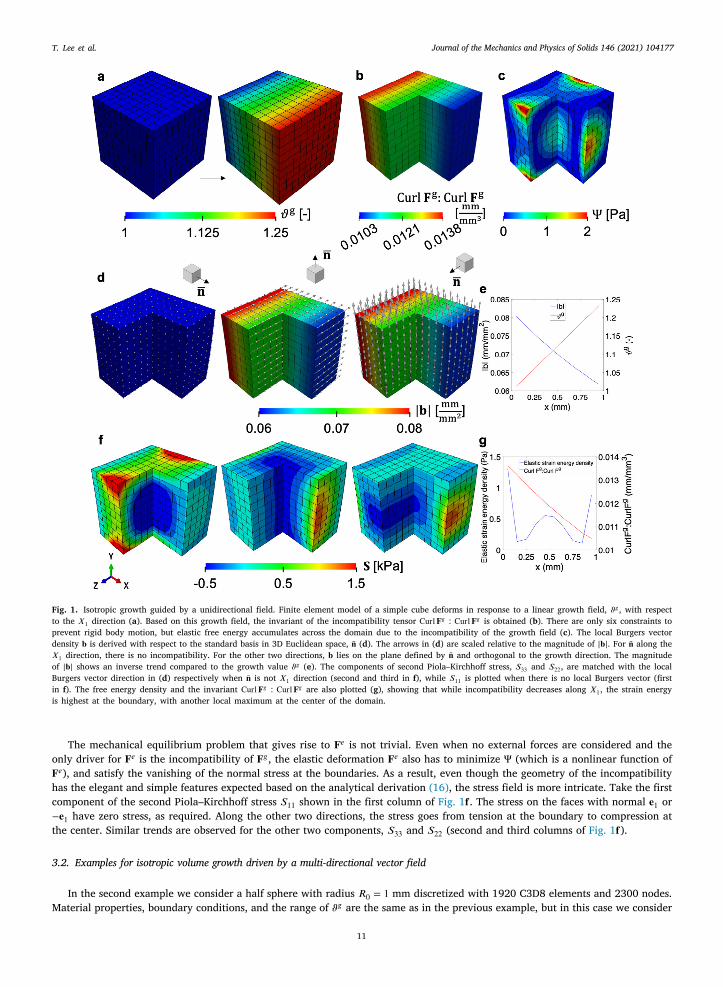
with time 𝑡 ∈ [0, 1]. This function leads to a 25% volume increase across the domain (Fig. 1𝐚). The growth field is non-uniform,howing a non-zero gradient in the direction of the 𝑋1 coordinate. The rationale for this field is to isolate a simple pattern of growthhat can be caused by a morphogen gradient for example.

The finite element model has 1331 nodes and we constrain only three translations and three rotations in order to allow freeeformation except for rigid body motions. Zero-traction natural boundary conditions are applied on all six boundary surfaces. Forhe material behavior we consider the neo-Hookean hyperelastic potential introduced before, with 𝜇 = 0.55 MPa (Lee et al., 2020)nd the initial compressibility 𝜈 = 0.4. Upon growth, the cube deforms solely due to growth into the configuration depicted inig. 1a. The contour plot in this panel is the growth variable 𝜗𝑔 , showing the desired gradient along 𝑋1.

The amount of incompatibility can be boiled down to the single invariant Curl𝐅𝑔 ∶ Curl𝐅𝑔 , which is motivated by similar scalarields in gradient plasticity related to energy stored as a consequence of crystal defects (Hurtado and Ortiz, 2013; Menzel andteinmann, 2000). While in our case the scalar field does not correspond to an energy quantity, it is an invariant field which overallelates to the degree of incompatibility and is therefore useful to visualize. The scalar Curl𝐅𝑔 ∶ Curl𝐅𝑔 changes in the same directionf the gradient of 𝜗𝑔 (Fig. 1b), which matches the intuition that incompatibility is related to mismatch between adjacent differentialolumes with different growth. Note, however, that even though the gradient of the volume change is constant, the incompatibilityetric is not. This occurs because even though the volume growth increases linearly with 𝑋1, the growth tensor is actually not a

inear function of 𝜗𝑔 . To achieve volume growth of 𝜗𝑔 , a differential volume element has to grow 3√

𝜗𝑔 in all directions.The local Burgers vector density 𝐛 can be calculated for any plane in the intermediate configuration. We choose the standard basis

n 3D Euclidean space as the normals of interest, e.g., �̄� = 𝐅𝑔𝐞1∕|𝐅𝑔𝐞1| and so on for the other two directions (Fig. 1𝐝). For the planecorresponding to the growth gradient, �̄� = 𝐅𝑔𝐞1∕|𝐅𝑔𝐞1|, the Burgers vector vanishes. This occurs because on the plane orthogonal tohe growth gradient, growth is uniform and therefore compatible. This follows directly from the definition of Curl𝐅𝑔 in Eq. (15).he local Burgers vector density in the other two planes is restricted to the corresponding plane. This was noted in the derivationf 𝐆 for the different growth types. In the case of isotropic growth fields it is always true that �̄�⊤𝐆�̄� = 0 for any normal �̄�. In thisxample it also becomes evident that 𝐛 is orthogonal to the growth gradient. The magnitude of the local Burgers vector density |𝐛|s also not constant over the domain (Fig. 1e). Instead, maybe albeit surprisingly, the magnitude is greater in the region with leastrowth, and decreases as growth increases. This can be explained by the fact that 𝐆 is scaled by the determinant of the permanentolume change. Even though on one end of the cube the growth is small, the relative difference in adjacent volume elements isreater in these regions compared to the relative mismatch in size between adjacent volume elements that have undergone moreubstantial growth.

To visualize the consequences of nonuniform growth on the development of residual stress, the second Piola–Kirchhoff stressensor 𝐒 is represented along each of the 𝐛 directions in Fig. 1𝐝 and the result is depicted in Fig. 1𝐟 . For the first panel of Fig. 1𝐟 ,ince the Burgers vector is not defined, we showed the first component of the second Piola–Kirchhoff stress 𝑆11. There are residualtresses in all three directions. The magnitude of the stress is not necessarily aligned with the magnitude of the local Burgers vectorensity. To get a better understanding of how the elastic deformation is distributed, Fig. 1𝐜 shows the contours of the elastic strain

𝑔 𝑔

10

nergy, and Fig. 1𝐠 compares the elastic strain energy against the scalar invariant of incompatibility Curl𝐅 ∶ Curl𝐅 .


Fig. 1. Isotropic growth guided by a unidirectional field. Finite element model of a simple cube deforms in response to a linear growth field, 𝜗𝑔 , with respectto the 𝑋1 direction (a). Based on this growth field, the invariant of the incompatibility tensor Curl𝐅𝑔 ∶ Curl𝐅𝑔 is obtained (b). There are only six constraints toprevent rigid body motion, but elastic free energy accumulates across the domain due to the incompatibility of the growth field (c). The local Burgers vectordensity 𝐛 is derived with respect to the standard basis in 3D Euclidean space, �̄� (d). The arrows in (d) are scaled relative to the magnitude of |𝐛|. For �̄� along the𝑋1 direction, there is no incompatibility. For the other two directions, 𝐛 lies on the plane defined by �̄� and orthogonal to the growth direction. The magnitudeof |𝐛| shows an inverse trend compared to the growth value 𝜗𝑔 (e). The components of second Piola–Kirchhoff stress, 𝑆33 and 𝑆22, are matched with the localBurgers vector direction in (d) respectively when �̄� is not 𝑋1 direction (second and third in f), while 𝑆11 is plotted when there is no local Burgers vector (firstin f). The free energy density and the invariant Curl𝐅𝑔 ∶ Curl𝐅𝑔 are also plotted (g), showing that while incompatibility decreases along 𝑋1, the strain energyis highest at the boundary, with another local maximum at the center of the domain.

The mechanical equilibrium problem that gives rise to 𝐅𝑒 is not trivial. Even when no external forces are considered and theonly driver for 𝐅𝑒 is the incompatibility of 𝐅𝑔 , the elastic deformation 𝐅𝑒 also has to minimize Ψ (which is a nonlinear function of𝐅𝑒), and satisfy the vanishing of the normal stress at the boundaries. As a result, even though the geometry of the incompatibilityhas the elegant and simple features expected based on the analytical derivation (16), the stress field is more intricate. Take the firstcomponent of the second Piola–Kirchhoff stress 𝑆11 shown in the first column of Fig. 1𝐟 . The stress on the faces with normal 𝐞1 or−𝐞1 have zero stress, as required. Along the other two directions, the stress goes from tension at the boundary to compression atthe center. Similar trends are observed for the other two components, 𝑆33 and 𝑆22 (second and third columns of Fig. 1𝐟).

3.2. Examples for isotropic volume growth driven by a multi-directional vector field

In the second example we consider a half sphere with radius 𝑅0 = 1 mm discretized with 1920 C3D8 elements and 2300 nodes.Material properties, boundary conditions, and the range of 𝜗𝑔 are the same as in the previous example, but in this case we consider

11


Ttt

t

lsI𝐛v

vmScw

wltr

3

tiahB

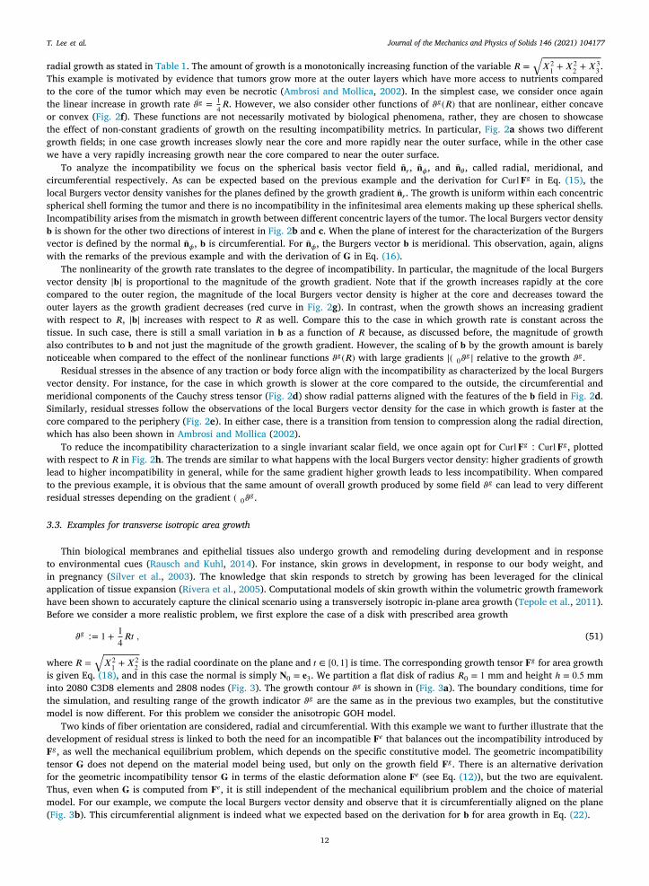
radial growth as stated in Table 1. The amount of growth is a monotonically increasing function of the variable 𝑅 =√

𝑋21 +𝑋2

2 +𝑋33 .

his example is motivated by evidence that tumors grow more at the outer layers which have more access to nutrients comparedo the core of the tumor which may even be necrotic (Ambrosi and Mollica, 2002). In the simplest case, we consider once againhe linear increase in growth rate 𝜗𝑔 = 1

4𝑅. However, we also consider other functions of 𝜗𝑔(𝑅) that are nonlinear, either concaveor convex (Fig. 2f). These functions are not necessarily motivated by biological phenomena, rather, they are chosen to showcasehe effect of non-constant gradients of growth on the resulting incompatibility metrics. In particular, Fig. 2a shows two different

growth fields; in one case growth increases slowly near the core and more rapidly near the outer surface, while in the other casewe have a very rapidly increasing growth near the core compared to near the outer surface.

To analyze the incompatibility we focus on the spherical basis vector field �̄�𝑟, �̄�𝜙, and �̄�𝜃 , called radial, meridional, andcircumferential respectively. As can be expected based on the previous example and the derivation for Curl𝐅𝑔 in Eq. (15), theocal Burgers vector density vanishes for the planes defined by the growth gradient �̄�𝑟. The growth is uniform within each concentricpherical shell forming the tumor and there is no incompatibility in the infinitesimal area elements making up these spherical shells.ncompatibility arises from the mismatch in growth between different concentric layers of the tumor. The local Burgers vector densityis shown for the other two directions of interest in Fig. 2b and c. When the plane of interest for the characterization of the Burgers

ector is defined by the normal �̄�𝜙, 𝐛 is circumferential. For �̄�𝜙, the Burgers vector 𝐛 is meridional. This observation, again, alignswith the remarks of the previous example and with the derivation of 𝐆 in Eq. (16).

The nonlinearity of the growth rate translates to the degree of incompatibility. In particular, the magnitude of the local Burgersvector density |𝐛| is proportional to the magnitude of the growth gradient. Note that if the growth increases rapidly at the corecompared to the outer region, the magnitude of the local Burgers vector density is higher at the core and decreases toward theouter layers as the growth gradient decreases (red curve in Fig. 2g). In contrast, when the growth shows an increasing gradientwith respect to 𝑅, |𝐛| increases with respect to 𝑅 as well. Compare this to the case in which growth rate is constant across thetissue. In such case, there is still a small variation in 𝐛 as a function of 𝑅 because, as discussed before, the magnitude of growthalso contributes to 𝐛 and not just the magnitude of the growth gradient. However, the scaling of 𝐛 by the growth amount is barelynoticeable when compared to the effect of the nonlinear functions 𝜗𝑔(𝑅) with large gradients |∇0𝜗𝑔| relative to the growth 𝜗𝑔 .

Residual stresses in the absence of any traction or body force align with the incompatibility as characterized by the local Burgersector density. For instance, for the case in which growth is slower at the core compared to the outside, the circumferential anderidional components of the Cauchy stress tensor (Fig. 2d) show radial patterns aligned with the features of the 𝐛 field in Fig. 2d.

imilarly, residual stresses follow the observations of the local Burgers vector density for the case in which growth is faster at theore compared to the periphery (Fig. 2e). In either case, there is a transition from tension to compression along the radial direction,hich has also been shown in Ambrosi and Mollica (2002).

To reduce the incompatibility characterization to a single invariant scalar field, we once again opt for Curl𝐅𝑔 ∶ Curl𝐅𝑔 , plottedith respect to 𝑅 in Fig. 2h. The trends are similar to what happens with the local Burgers vector density: higher gradients of growth

ead to higher incompatibility in general, while for the same gradient higher growth leads to less incompatibility. When comparedo the previous example, it is obvious that the same amount of overall growth produced by some field 𝜗𝑔 can lead to very differentesidual stresses depending on the gradient ∇0𝜗𝑔 .

.3. Examples for transverse isotropic area growth

Thin biological membranes and epithelial tissues also undergo growth and remodeling during development and in responseo environmental cues (Rausch and Kuhl, 2014). For instance, skin grows in development, in response to our body weight, andn pregnancy (Silver et al., 2003). The knowledge that skin responds to stretch by growing has been leveraged for the clinicalpplication of tissue expansion (Rivera et al., 2005). Computational models of skin growth within the volumetric growth frameworkave been shown to accurately capture the clinical scenario using a transversely isotropic in-plane area growth (Tepole et al., 2011).efore we consider a more realistic problem, we first explore the case of a disk with prescribed area growth

𝜗𝑔 ∶= 1 + 14𝑅𝑡 , (51)

where 𝑅 =√

𝑋21 +𝑋2

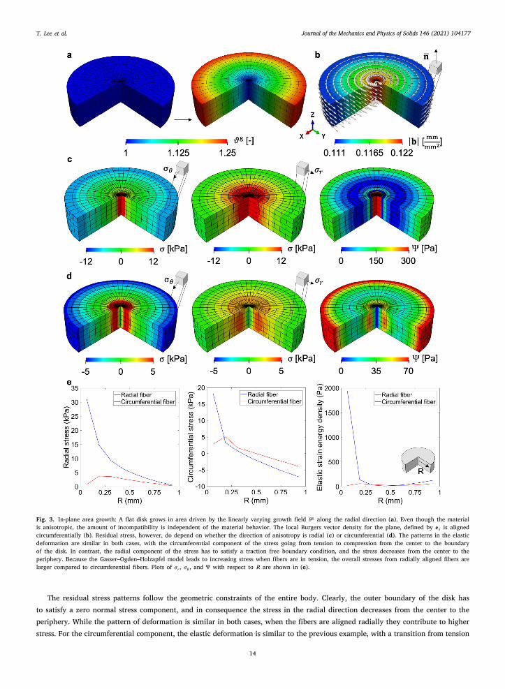
2 is the radial coordinate on the plane and 𝑡 ∈ [0, 1] is time. The corresponding growth tensor 𝐅𝑔 for area growthis given Eq. (18), and in this case the normal is simply 𝐍0 = 𝐞3. We partition a flat disk of radius 𝑅0 = 1 mm and height ℎ = 0.5 mminto 2080 C3D8 elements and 2808 nodes (Fig. 3). The growth contour 𝜗𝑔 is shown in (Fig. 3a). The boundary conditions, time forthe simulation, and resulting range of the growth indicator 𝜗𝑔 are the same as in the previous two examples, but the constitutivemodel is now different. For this problem we consider the anisotropic GOH model.

Two kinds of fiber orientation are considered, radial and circumferential. With this example we want to further illustrate that thedevelopment of residual stress is linked to both the need for an incompatible 𝐅𝑒 that balances out the incompatibility introduced by𝐅𝑔 , as well the mechanical equilibrium problem, which depends on the specific constitutive model. The geometric incompatibilitytensor 𝐆 does not depend on the material model being used, but only on the growth field 𝐅𝑔 . There is an alternative derivationfor the geometric incompatibility tensor 𝐆 in terms of the elastic deformation alone 𝐅𝑒 (see Eq. (12)), but the two are equivalent.Thus, even when 𝐆 is computed from 𝐅𝑒, it is still independent of the mechanical equilibrium problem and the choice of materialmodel. For our example, we compute the local Burgers vector density and observe that it is circumferentially aligned on the plane(Fig. 3b). This circumferential alignment is indeed what we expected based on the derivation for 𝐛 for area growth in Eq. (22).

12


Fig. 2. Isotropic volume growth guided by a multi-directional field with different growth distributions: an increasing gradient of 𝜗𝑔 from the inner core to theouter shell (a, left) and a case in which 𝜗𝑔 increases rapidly at the core and slowly at the outer layers (a, right). The local Burgers vector density is computedfor each of the two cases and for planes defined by the spherical basis vector corresponding to meridional and circumferential directions �̄�𝜙 and �̄�𝜃 . (b, c). TheBurgers vector vanishes for planes defined by the radial direction �̄�𝑟 and are thus not shown. Stress components aligned with the direction of the Burgers vectorsshow similar trends to the degree of incompatibility for the two cases considered (d, e). The growth fields considered, in addition to the two cases illustratedin the top panels, are shown in f, were the blue curve is the case shown in the left column of a, and the red curve is the right column of a. The magnitudeof the local Burgers vector density |𝐛| is greater for higher growth gradients, but also greater for smaller growth values (g). The scalar metric Curl𝐅𝑔 ∶ Curl𝐅𝑔shows the same trends as the magnitude of the local Burgers vector density (h).

Even though the growth field and incompatibility metrics remain the same, the residual stresses change if the GOH materialis considered with a radial fiber family (Fig. 3c) or circumferential fiber family (Fig. 3d). We report the circumferential stress 𝜎𝜃 ,radial stress 𝜎𝑟, and free energy density Ψ. When the fiber is radially distributed, stress along fiber direction is higher than thestress in the circumferential direction (Fig. 3c). The radial component of the stress is in tension and the stress is higher at the centercompared to the periphery of the disk, where it vanishes because of the boundary condition. The circumferential direction followsa more similar pattern compared to the previous cases, with tension at the center and gradually transitioning to compression at theouter layers just as in the simple tumor example. If the fiber orientation is circumferential, the trends in the stress are similar butoverall the stresses and strain energy are lower, particularly due to the lack of fibers in tension in the radial direction (Fig. 3d).

13


Fig. 3. In-plane area growth: A flat disk grows in area driven by the linearly varying growth field 𝜗𝑔 along the radial direction (a). Even though the materialis anisotropic, the amount of incompatibility is independent of the material behavior. The local Burgers vector density for the plane, defined by 𝐞3 is alignedcircumferentially (b). Residual stress, however, do depend on whether the direction of anisotropy is radial (c) or circumferential (d). The patterns in the elasticdeformation are similar in both cases, with the circumferential component of the stress going from tension to compression from the center to the boundaryof the disk. In contrast, the radial component of the stress has to satisfy a traction free boundary condition, and the stress decreases from the center to theperiphery. Because the Gasser–Ogden–Holzapfel model leads to increasing stress when fibers are in tension, the overall stresses from radially aligned fibers arelarger compared to circumferential fibers. Plots of 𝜎𝑟, 𝜎𝜃 , and Ψ with respect to 𝑅 are shown in (e).

The residual stress patterns follow the geometric constraints of the entire body. Clearly, the outer boundary of the disk hasto satisfy a zero normal stress component, and in consequence the stress in the radial direction decreases from the center to theperiphery. While the pattern of deformation is similar in both cases, when the fibers are aligned radially they contribute to higherstress. For the circumferential component, the elastic deformation is similar to the previous example, with a transition from tension

14


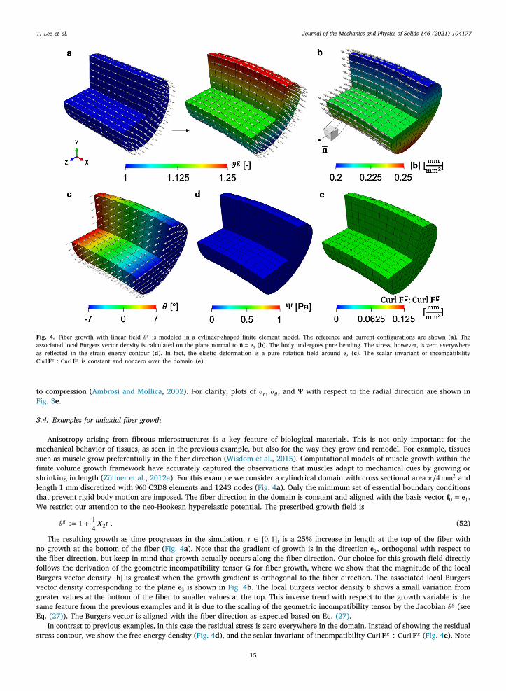
Fig. 4. Fiber growth with linear field 𝜗𝑔 is modeled in a cylinder-shaped finite element model. The reference and current configurations are shown (a). Theassociated local Burgers vector density is calculated on the plane normal to �̄� = 𝐞3 (b). The body undergoes pure bending. The stress, however, is zero everywhereas reflected in the strain energy contour (d). In fact, the elastic deformation is a pure rotation field around 𝐞3 (c). The scalar invariant of incompatibilityCurl𝐅𝑔 ∶ Curl𝐅𝑔 is constant and nonzero over the domain (e).

to compression (Ambrosi and Mollica, 2002). For clarity, plots of 𝜎𝑟, 𝜎𝜃 , and Ψ with respect to the radial direction are shown inFig. 3e.

3.4. Examples for uniaxial fiber growth

Anisotropy arising from fibrous microstructures is a key feature of biological materials. This is not only important for themechanical behavior of tissues, as seen in the previous example, but also for the way they grow and remodel. For example, tissuessuch as muscle grow preferentially in the fiber direction (Wisdom et al., 2015). Computational models of muscle growth within thefinite volume growth framework have accurately captured the observations that muscles adapt to mechanical cues by growing orshrinking in length (Zöllner et al., 2012a). For this example we consider a cylindrical domain with cross sectional area 𝜋∕4mm2 andlength 1 mm discretized with 960 C3D8 elements and 1243 nodes (Fig. 4a). Only the minimum set of essential boundary conditionsthat prevent rigid body motion are imposed. The fiber direction in the domain is constant and aligned with the basis vector 𝐟0 = 𝐞1.We restrict our attention to the neo-Hookean hyperelastic potential. The prescribed growth field is

𝜗𝑔 ∶= 1 + 14𝑋2𝑡 . (52)

The resulting growth as time progresses in the simulation, 𝑡 ∈ [0, 1], is a 25% increase in length at the top of the fiber withno growth at the bottom of the fiber (Fig. 4a). Note that the gradient of growth is in the direction 𝐞2, orthogonal with respect tothe fiber direction, but keep in mind that growth actually occurs along the fiber direction. Our choice for this growth field directlyfollows the derivation of the geometric incompatibility tensor 𝐆 for fiber growth, where we show that the magnitude of the localBurgers vector density |𝐛| is greatest when the growth gradient is orthogonal to the fiber direction. The associated local Burgersvector density corresponding to the plane 𝐞3 is shown in Fig. 4b. The local Burgers vector density 𝐛 shows a small variation fromgreater values at the bottom of the fiber to smaller values at the top. This inverse trend with respect to the growth variable is thesame feature from the previous examples and it is due to the scaling of the geometric incompatibility tensor by the Jacobian 𝜗𝑔 (seeEq. (27)). The Burgers vector is aligned with the fiber direction as expected based on Eq. (27).

In contrast to previous examples, in this case the residual stress is zero everywhere in the domain. Instead of showing the residualstress contour, we show the free energy density (Fig. 4d), and the scalar invariant of incompatibility Curl𝐅𝑔 ∶ Curl𝐅𝑔 (Fig. 4e). Note

15


c

T

Td

t

3

ladwaia

bt

uda

wteniof

3

Temi

that there is incompatibility induced by the growth field, and that the cylinder deforms due to the prescribed growth. Yet, there isno residual stress. Recall that the elastic deformation tensor should counteract the incompatibility introduced by 𝐅𝑔 . However, thepolar decomposition of 𝐅𝑒 in Eq. (4) reveals that a pure rotation field could be able to get a globally compatible 𝐅 with no stress.This is in fact what is happening here. In matrix form, using the Cartesian basis, the growth tensor is

𝐅𝑔 =⎡

⎢

⎢

⎣

1 + 𝑎𝑋2 0 00 1 00 0 1

⎤

⎥

⎥

⎦

, (53)

for some non-zero value 𝑎. This growth field is incompatible as illustrated in Fig. 4b and e. We propose that the elastic deformationan be a rotation 𝐅𝑒 = 𝐑𝑒. We suggest this solution expressed in matrix form

𝐅𝑒 =⎡

⎢

⎢

⎣

cos 𝜃 sin 𝜃 0− sin 𝜃 cos 𝜃 0

0 0 1

⎤

⎥

⎥

⎦

. (54)

his rotation should be such that the total deformation 𝐅 = 𝐅𝑔𝐅𝑒 is compatible. The total deformation gradient is

𝐅 =⎡

⎢

⎢

⎣

(1 + 𝑎𝑋2) cos 𝜃 sin 𝜃 0−(1 + 𝑎𝑋2) sin 𝜃 cos 𝜃 0

0 0 1

⎤

⎥

⎥

⎦

. (55)

o show that this is the case, all we need to do is to show that there is a vector field whose gradient leads to Eq. (55). Consider theeformation map

𝝋 =(

𝑋2 sin(𝑎𝑋1) +1𝑎sin(𝑎𝑋1), 𝑋2 cos(𝑎𝑋1) +

1𝑎cos(𝑎𝑋1), 𝑋3

)

. (56)

The deformation gradient 𝐅 in Eq. (55) is actually the gradient of the map 𝝋 in Eq. (56), with 𝜃 = 𝑎𝑋1. Furthermore, this has tobe the solution of the problem since, by reducing to a rotation, 𝐅𝑒 leads to zero stress while also satisfying mechanical equilibrium.Numerically, Fig. 4c shows that the elastic deformation 𝐅𝑒 from our finite element solution is actually a pure rotation around 𝐞3hat varies along 𝑋1 as expected.

.5. Brain atrophy

Commonly, the idea of tissue growth is associated with an increase in mass; however, as noted after introducing Eq. (3), volumeoss can also be considered, as in the case of tissue atrophy. A representative example is atrophy and shrinkage of the brain as

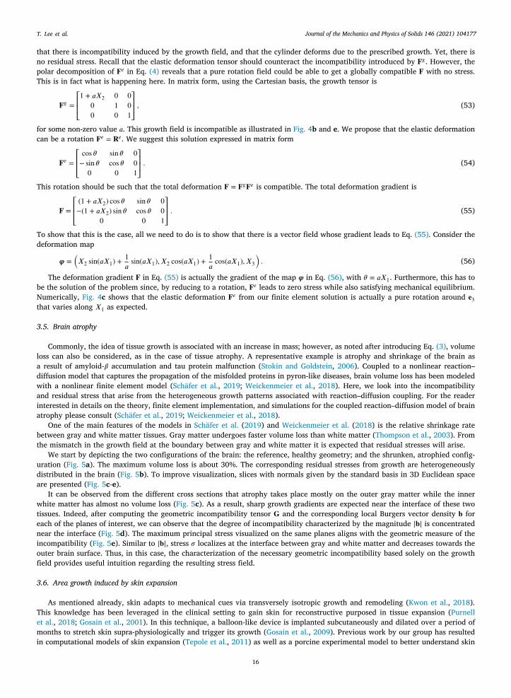
result of amyloid-𝛽 accumulation and tau protein malfunction (Stokin and Goldstein, 2006). Coupled to a nonlinear reaction–iffusion model that captures the propagation of the misfolded proteins in pyron-like diseases, brain volume loss has been modeledith a nonlinear finite element model (Schäfer et al., 2019; Weickenmeier et al., 2018). Here, we look into the incompatibilitynd residual stress that arise from the heterogeneous growth patterns associated with reaction–diffusion coupling. For the readernterested in details on the theory, finite element implementation, and simulations for the coupled reaction–diffusion model of braintrophy please consult (Schäfer et al., 2019; Weickenmeier et al., 2018).

One of the main features of the models in Schäfer et al. (2019) and Weickenmeier et al. (2018) is the relative shrinkage rateetween gray and white matter tissues. Gray matter undergoes faster volume loss than white matter (Thompson et al., 2003). Fromhe mismatch in the growth field at the boundary between gray and white matter it is expected that residual stresses will arise.

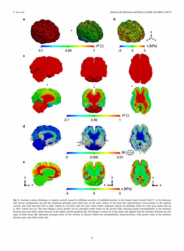
We start by depicting the two configurations of the brain: the reference, healthy geometry; and the shrunken, atrophied config-ration (Fig. 5a). The maximum volume loss is about 30%. The corresponding residual stresses from growth are heterogeneouslyistributed in the brain (Fig. 5b). To improve visualization, slices with normals given by the standard basis in 3D Euclidean spacere presented (Fig. 5c-e).

It can be observed from the different cross sections that atrophy takes place mostly on the outer gray matter while the innerhite matter has almost no volume loss (Fig. 5c). As a result, sharp growth gradients are expected near the interface of these two

issues. Indeed, after computing the geometric incompatibility tensor 𝐆 and the corresponding local Burgers vector density 𝐛 forach of the planes of interest, we can observe that the degree of incompatibility characterized by the magnitude |𝐛| is concentratedear the interface (Fig. 5d). The maximum principal stress visualized on the same planes aligns with the geometric measure of thencompatibility (Fig. 5e). Similar to |𝐛|, stress 𝜎 localizes at the interface between gray and white matter and decreases towards theuter brain surface. Thus, in this case, the characterization of the necessary geometric incompatibility based solely on the growthield provides useful intuition regarding the resulting stress field.

.6. Area growth induced by skin expansion

As mentioned already, skin adapts to mechanical cues via transversely isotropic growth and remodeling (Kwon et al., 2018).his knowledge has been leveraged in the clinical setting to gain skin for reconstructive purposed in tissue expansion (Purnellt al., 2018; Gosain et al., 2001). In this technique, a balloon-like device is implanted subcutaneously and dilated over a period ofonths to stretch skin supra-physiologically and trigger its growth (Gosain et al., 2009). Previous work by our group has resulted

16

n computational models of skin expansion (Tepole et al., 2011) as well as a porcine experimental model to better understand skin


Fig. 5. Isotropic volume shrinkage or negative growth caused by diffusion–reaction of misfolded proteins in the human brain: Growth field 𝜗𝑔 in the referenceand current configuration (a) and the maximum principal stress field seen on the outer surface of the brain (b). Representative cross-sections in the sagittal,coronal, and axial direction (left to right column in c–e) show that the inner white matter undergoes almost no shrinkage while the outer gray matter has upto 30% volume loss (c). The local Burgers vector density can be calculated solely based on the growth field, showing greater incompatibility at the interfacebetween gray and white matter because of the higher growth gradients (d). The Burgers vectors are in the plane and aligned with the interface between the twotypes of brain tissue (d). Maximum principal stress on the sections of interest reflects the incompatibility characterization, with greater stress at the interfacebetween gray and white matter (e).

17


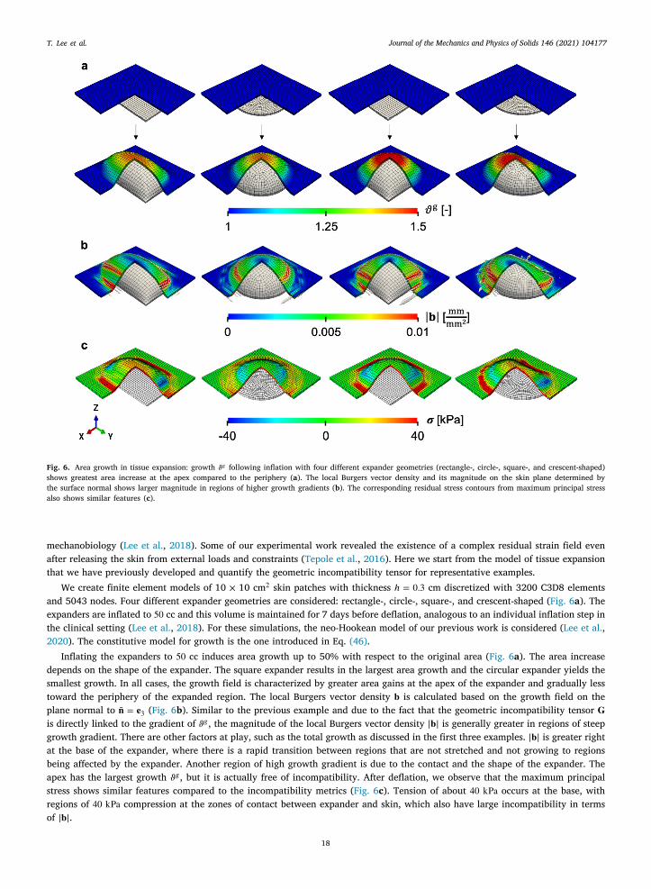
Fig. 6. Area growth in tissue expansion: growth 𝜗𝑔 following inflation with four different expander geometries (rectangle-, circle-, square-, and crescent-shaped)shows greatest area increase at the apex compared to the periphery (a). The local Burgers vector density and its magnitude on the skin plane determined bythe surface normal shows larger magnitude in regions of higher growth gradients (b). The corresponding residual stress contours from maximum principal stressalso shows similar features (c).

mechanobiology (Lee et al., 2018). Some of our experimental work revealed the existence of a complex residual strain field evenafter releasing the skin from external loads and constraints (Tepole et al., 2016). Here we start from the model of tissue expansionthat we have previously developed and quantify the geometric incompatibility tensor for representative examples.

We create finite element models of 10 × 10 cm2 skin patches with thickness ℎ = 0.3 cm discretized with 3200 C3D8 elementsand 5043 nodes. Four different expander geometries are considered: rectangle-, circle-, square-, and crescent-shaped (Fig. 6a). Theexpanders are inflated to 50 cc and this volume is maintained for 7 days before deflation, analogous to an individual inflation step inthe clinical setting (Lee et al., 2018). For these simulations, the neo-Hookean model of our previous work is considered (Lee et al.,2020). The constitutive model for growth is the one introduced in Eq. (46).

Inflating the expanders to 50 cc induces area growth up to 50% with respect to the original area (Fig. 6a). The area increasedepends on the shape of the expander. The square expander results in the largest area growth and the circular expander yields thesmallest growth. In all cases, the growth field is characterized by greater area gains at the apex of the expander and gradually lesstoward the periphery of the expanded region. The local Burgers vector density 𝐛 is calculated based on the growth field on theplane normal to �̄� = 𝐞3 (Fig. 6b). Similar to the previous example and due to the fact that the geometric incompatibility tensor 𝐆is directly linked to the gradient of 𝜗𝑔 , the magnitude of the local Burgers vector density |𝐛| is generally greater in regions of steepgrowth gradient. There are other factors at play, such as the total growth as discussed in the first three examples. |𝐛| is greater rightat the base of the expander, where there is a rapid transition between regions that are not stretched and not growing to regionsbeing affected by the expander. Another region of high growth gradient is due to the contact and the shape of the expander. Theapex has the largest growth 𝜗𝑔 , but it is actually free of incompatibility. After deflation, we observe that the maximum principalstress shows similar features compared to the incompatibility metrics (Fig. 6c). Tension of about 40 kPa occurs at the base, withregions of 40 kPa compression at the zones of contact between expander and skin, which also have large incompatibility in termsof |𝐛|.

18


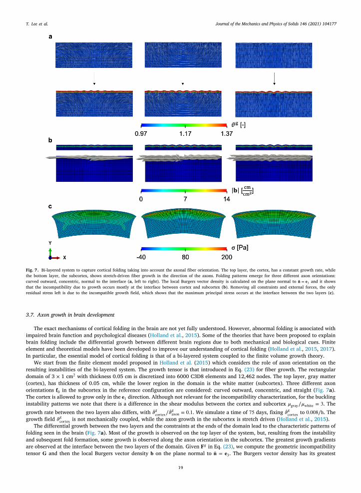
Fig. 7. Bi-layered system to capture cortical folding taking into account the axonal fiber orientation. The top layer, the cortex, has a constant growth rate, whilethe bottom layer, the subcortex, shows stretch-driven fiber growth in the direction of the axons. Folding patterns emerge for three different axon orientations:curved outward, concentric, normal to the interface (a, left to right). The local Burgers vector density is calculated on the plane normal to �̄� = 𝐞3 and it showsthat the incompatibility due to growth occurs mostly at the interface between cortex and subcortex (b). Removing all constraints and external forces, the onlyresidual stress left is due to the incompatible growth field, which shows that the maximum principal stress occurs at the interface between the two layers (c).

3.7. Axon growth in brain development

The exact mechanisms of cortical folding in the brain are not yet fully understood. However, abnormal folding is associated withimpaired brain function and psychological diseases (Holland et al., 2015). Some of the theories that have been proposed to explainbrain folding include the differential growth between different brain regions due to both mechanical and biological cues. Finiteelement and theoretical models have been developed to improve our understanding of cortical folding (Holland et al., 2015, 2017).In particular, the essential model of cortical folding is that of a bi-layered system coupled to the finite volume growth theory.

We start from the finite element model proposed in Holland et al. (2015) which considers the role of axon orientation on theresulting instabilities of the bi-layered system. The growth tensor is that introduced in Eq. (23) for fiber growth. The rectangulardomain of 3 × 1 cm2 with thickness 0.05 cm is discretized into 6000 C3D8 elements and 12,462 nodes. The top layer, gray matter(cortex), has thickness of 0.05 cm, while the lower region in the domain is the white matter (subcortex). Three different axonorientations 𝐟0 in the subcortex in the reference configuration are considered: curved outward, concentric, and straight (Fig. 7a).The cortex is allowed to grow only in the 𝐞1 direction. Although not relevant for the incompatibility characterization, for the bucklinginstability patterns we note that there is a difference in the shear modulus between the cortex and subcortex 𝜇gray∕𝜇white = 3. Thegrowth rate between the two layers also differs, with �̇�𝑔cortex∕�̇�

𝑔axon = 0.1. We simulate a time of 75 days, fixing �̇�𝑔cortex to 0.008∕h. The

growth field 𝜗𝑔cortex is not mechanically coupled, while the axon growth in the subcortex is stretch driven (Holland et al., 2015).The differential growth between the two layers and the constraints at the ends of the domain lead to the characteristic patterns of

folding seen in the brain (Fig. 7a). Most of the growth is observed on the top layer of the system, but, resulting from the instabilityand subsequent fold formation, some growth is observed along the axon orientation in the subcortex. The greatest growth gradientsare observed at the interface between the two layers of the domain. Given 𝐅𝑔 in Eq. (23), we compute the geometric incompatibilitytensor 𝐆 and then the local Burgers vector density 𝐛 on the plane normal to �̄� = 𝐞 . The Burgers vector density has its greatest

19

3


et

magnitude precisely at the interface between the cortex and subcortex, where the gradient of growth is sharpest. This is the expectedbehavior of the system. The ideal scenario in which no axon growth is considered but only differential isotropic growth betweenthe two layers is allowed, would lead to zero incompatibility in either region. In that case, the incompatibility would be completelyrestricted to a singular region of non-zero incompatibility exactly at the interface. In that case, folds would still form, and the causefor residual stress would be the mismatch along the interface of the two layers (Budday et al., 2014). In fact, an experimentalconfirmation is presented in Budday et al. (2017), where two thin strips of elastomers are deformed elastically to a different extent(and therefore without any incompatibility) and then glued together. The bi-layered system shows the expected instabilities andbuckling patterns, but in the end the only source of incompatibility is precisely at the interface. In our example, incorporating theaxon orientation and growth leads to Burgers vectors mostly aligned with the interface (Fig. 7b). The direction of the axons doesaffect the pattern and magnitude of |𝐛|, as the gradient between cortex and subcortex is greater when the axons are normal to thecortex (second and third columns in Fig. 7a), as opposed to the case in which axons approach the interface tangentially (first columnin Fig. 7a).

The buckling patterns typical of the folded brain exist because of the constraints applied to the system, which is fixed at bothnds. We are interested in the residual stress patterns when there are no external loads and the only constraints imposed are thosehat prevent rigid body motion. The residual stress field that arises solely by the incompatibility is shown in Fig. 7c. We restrict

our attention to the maximum principal stress. There is peak tension at the subcortex right below the interface with the cortex.This is particularly noticeable for the cases in which the axon orientation is normal to the interface. For the case in which the axonorientation is tangential to the interface, the incompatibility is less pronounced and the residual stress is also much lower. Movingaway from the interface, the stress decreases. In the cortex, stresses are actually very small. The growth in the cortex is uniformand this layer is stiffer that the subcortex. As a result, releasing all constraints on the system leads to a constant bending of the toplayer. This overall bending exerts the tensile stresses at the top of the softer subcortex, with small variations corresponding to thegrowth field in the axon direction. Yet, as stated before, the variations in the growth field within the subcortex are small comparedto near the interface with the cortex.

4. Discussion

The exact microscopic origin of residual stress in soft tissues is still an open question. However, it is generally accepted thatthe pre-stress field at the macroscopic level is a consequence of the constant growth and remodeling of living matter (Ambrosiet al., 2011; Humphrey and Rajagopal, 2002; Taber and Humphrey, 2001). Growth and remodeling can be captured within acontinuum mechanics framework in a manner akin to plasticity by splitting the deformation gradient into growth and elasticcontributions (Lee, 1969; Rodriguez et al., 1994). This split is linked to the idea of incompatibility (Skalak et al., 1996), a notionof mismatch and discontinuity between differential volume elements at the microscopic scale. In crystal plasticity, these conceptsare linked to lattice defects. Although the interpretation is not the same for soft tissues, we borrow from the concepts of crystalplasticity to describe the kinematics of incompatibility due to growth. Through this paper, we have presented the distinctive featuresof the geometric incompatibility tensor that exist for three general growth formulations: volume, area, and fiber growth. We alsocompute the geometrically necessary incompatibility for three realistic biomedical problems. Although we focus on the geometryof incompatibility, we show that some features of the residual stress field are closely related to the incompatibility field.

The primary object of the present work was to introduce the geometric incompatibility tensor 𝐆 in the context of growth andremodeling. This tensor is based on the definition of the Burgers vector, which is a measure of the failure to close circuits in asurface after the application of the irreversible deformation 𝐅𝑔 . The generalization of the Burgers vector calculation for any normal𝐧, together with a localization argument, yields the tensor 𝐆, which is closely related to the Curl operator. In the finite volume growththeory, the tensor 𝐅𝑔 is constrained by the biology and by the anatomy or microstructure of the tissue. Growth is also connected tothe thermodynamic balance laws which connect the tensor 𝐅𝑔 to the scalar mass source. These constraints on 𝐅𝑔 allow us to derivespecific features of 𝐆 for different growth modes. The most prominent feature is that the degree and direction of incompatibilitydepend on the magnitude and direction of the growth gradient. There are more subtle features that were discussed for the individualgrowth models.

To better understand these incompatible fields we started with very simple illustrative examples. A key task in our manuscriptwas the numerical implementation of the different growth problems and the subsequent calculation of the incompatibility metricswithin the finite element framework. To that end, we were able to compare our simulations against the analytical derivations. Thefinite element calculations further cemented some of the observations about 𝐆 and the local Burgers vector density 𝐛. For example,the simpler problems confirmed that there is no incompatibility in the direction of the growth gradient, and that for a given planedefined by normal 𝐧 the Burgers vector has to lie in that plane. In contrast, we did not devote much attention to the residual stressresulting from the incompatible growth field. The stress field is more complex because there are several factors that come intoplay beyond the geometry of the permanent deformation. Clearly the 𝐅𝑒 field is generally dependent on the overall geometry andboundary conditions (Ambrosi and Mollica, 2002). That being said, our numerical implementation naturally delivers the residualstresses in our simulations and allows us a side by side comparison of incompatibility patterns and the resulting stress field. Thelast of the representative examples allowed us to showcase that there are incompatible growth fields that do not lead to stress,something that is better understood for crystals (Nye, 1953). In our fiber growth example we showed how a pure rotation 𝐅𝑒 = 𝐑𝑒which is incompatible is sufficient to obtain a total deformation that is compatible but entails no residual stress.

Our idealized problems enabled us to point out the distinctive features of the geometry of incompatibility and to showcase the

20

finite element implementation (which we make available with this manuscript). Yet, we are interested in understanding how these


cPr

foReSagpech

imelu2ncapttdi

5

iiats

C

WT

D

t

incompatible fields look like in realistic applications. We know that residual stress is a feature of living tissue and that it is importantfor function (Fung, 1991). Hence, having presented our tools, we applied them to three relevant biomedical questions. In the brain,for example, we observed that the gradient of growth during development and atrophy is highest at the interface between whiteand gray matter, and this is the region with the highest degree of incompatibility and also residual stress. The perfect experimentalanalogy of an ideal system is the work by Budday et al. (2017), where the compatible deformation of two layers before being gluedtogether leads to residual stress due to the mismatch of deformation at the interface. Our numerical example in the brain addsadditional complexities compared to the idealized experiment. For example, the growth of axons in the white matter can increaseor decrease the degree of incompatibility depending on their orientation with respect to the interface.

From the tissue expansion simulations we also gained valuable insights. It has been discussed in previous computational models,linical experience, and animal experiments, that there is more growth at the apex compared to the periphery (Tepole et al., 2015;urnell et al., 2018). Here we show that, in fact, the residual stress is highest at the periphery and at the beginning of the contactegion between expander and skin. These regions coincide with the sharpest gradients of growth and our incompatibility metrics.

In the illustrative examples at the beginning of the Results, and the biomedical applications that we present afterwards, we haveocused on characterizing the type of geometry associated with growth and remodeling. As pointed out in the introduction, thepposite question is also of utmost interest: Can the constitutive equation for the growth rate take into account incompatibility?esidual stress has indeed been proposed as a key regulator in development of plants and animals (Ciarletta et al., 2016; Rebochot al., 2017). An initial exploration into this question through the lens of the incompatible configurations is presented in theupplemental material, where we show conditions on the growth profile that can lead to constant magnitude of the Burgers vectorlong the growth gradient. A direct dependence on 𝐆 in Eq. (44) is one possible way of connecting the geometric defects due torowth to the growth process itself. Another phenomenon worth discussing is that cellular mechanobiology is most likely not a localhenomenon. Mechanobiology pathways for connective tissue include the production and diffusion of growth factors (Humphreyt al., 2014; Sree and Tepole, 2020). Due to the presence of diffusion of these coupled fields, it is reasonable to anticipate thatonsideration of growth factors will impact growth gradients and, consequently, the incompatibility metrics. Such analysis is,owever, beyond the scope of this paper.

This work is not without limitations. One of the open questions in this work is the precise connection between the geometry ofncompatibility and the residual stress. While the metrics introduced do align in general with the development of residual stress,ore work is needed to elucidate this relationship in more detail. An area of future research in this regard is to understand the

ffect of material properties on the development of residual stress, especially for the mechanically-coupled problems. The other mainimitation is that we have fully focused on the split of the deformation gradient into growth and elastic contributions. This approach isseful in practice, describes growth and remodeling accurately, and is amenable to efficient finite element implementations (Holland,018). However, comparison against other descriptions of growth and remodeling is our future endeavor, such as the evolution ofatural configurations for individual constituents (Humphrey and Rajagopal, 2002), or the notion of a higher-dimensional referenceonfiguration (Tomassetti et al., 2016; Abi-Akl and Cohen, 2020). Furthermore, the multiplicative split into a single pair of growthnd elastic deformations is a valid representation of the final state of residual stress in the tissue, but does not capture the dynamicrocess of growth as a sequence of incremental growth and elastic deformations. This last point connects to one open questionhat we will also continue to investigate in the near future: what is the connection between the geometry of incompatibility andhe microscale remodeling for soft tissues? As we stated repeatedly in the manuscript, soft tissues do not have lattice defects orislocations. While our analysis is useful at the continuum scale, it leaves unanswered the microscopic and molecular origin ofncompatibility in living matter.

. Conclusions

Within the finite volume growth framework, residual stress arises due to the incompatibility of the growth field. Here we exploren detail the geometric characterization of this incompatibility. We implement the calculations of growing tissues and the geometricncompatibility tensor 𝐆 into a nonlinear finite element framework. We showcased idealized scenarios and also relevant biomedicalpplications. Therefore, we expect that this work will further our insight into the origin and characterization of residual stress in softissue, which can be instrumental in understanding disease and designing clinical interventions in which growth and remodeling ofoft tissue plays a central role.

RediT authorship contribution statement

Taeksang Lee: Conceptualization, Methodology, Software, Formal analysis, Writing. Maria A. Holland: Software, Resources,riting. Johannes Weickenmeier: Software, Resources, Writing. Arun K. Gosain: Conceptualization, Writing. Adrian Buganzaepole: Conceptualization, Methodology, Formal analysis, Writing, Supervision.

eclaration of competing interest

The authors declare that they have no known competing financial interests or personal relationships that could have appearedo influence the work reported in this paper.

21


UU

S

R

AA

ABBBBCCCC

CDD

E

EEFF

FFGG

G

G

G

G

HHHHHHHH

J

KK

KKK

KKK

L

Acknowledgments

This work was supported by the National Institute of Arthritis and Musculoskeletal and Skin Diseases, National Institute of Health,nited States under award R01AR074525 to Adrian Buganza and by the National Institute on Aging, National Institute of Health,nited States under award R21AG067442 to Johannes Weickenmeier.

upplementary material

Code associated with this publication can be accessed at https://bitbucket.org/abuganzatepole/incompatibilityfe.

eferences

bi-Akl, R., Cohen, T., 2020. Surface growth on a deformable spherical substrate. Mech. Res. Commun. 103.mbrosi, D., Ateshian, G.A., Arruda, E.M., Cowin, S., Dumais, J., Goriely, A., Holzapfel, G.A., Humphrey, J.D., Kemkemer, R., Kuhl, E., et al., 2011. Perspectives

on biological growth and remodeling. J. Mech. Phys. Solids 59 (4), 863–883.mbrosi, D., Mollica, F., 2002. On the mechanics of a growing tumor. Internat. J. Engrg. Sci. 40 (12), 1297–1316.ray, D., 1984. Axonal growth in response to experimentally applied mechanical tension. Dev. Biol. 102 (2), 379–389.rown, I.A., 1973. A scanning electron microscope study of the effects of uniaxial tension on human skin. Br. J. Dermatol. 89 (4), 383–393.udday, S., Andres, S., Walter, B., Steinmann, P., Kuhl, E., 2017. Wrinkling instabilities in soft bilayered systems. Phil. Trans. R. Soc. A 375 (2093), 20160163.udday, S., Steinmann, P., Kuhl, E., 2014. The role of mechanics during brain development. J. Mech. Phys. Solids 72, 75–92.ermelli, P., Gurtin, M.E., 2001. On the characterization of geometrically necessary dislocations in finite plasticity. J. Mech. Phys. Solids 49 (7), 1539–1568.huong, C.-J., Fung, Y.-C., 1986. Residual stress in arteries. In: Frontiers in Biomechanics. Springer, pp. 117–129.iarletta, P., 2013. Buckling instability in growing tumor spheroids. Phys. Rev. Lett. 110 (15), 158102.iarletta, P., Destrade, M., Gower, A.L., 2016. On residual stresses and homeostasis: an elastic theory of functional adaptation in living matter. Sci. Rep. 6,

24390.layton, J.D., Bammann, D.J., McDowell, D.L., 2005. A geometric framework for the kinematics of crystals with defects. Phil. Mag. 85 (33–35), 3983–4010.aly, C.H., 1982. Biomechanical properties of dermis. J. Investig. Dermatol. 79 (1), 17–20.e Wit, R., 1981. A view of the relation between the continuum theory of lattice defects and non-Euclidean geometry in the linear approximation. Internat. J.

Engrg. Sci. 19 (12), 1475–1506.chevin, E., Le Gloanec, C., Skowrońska, N., Routier-Kierzkowska, A.-L., Burian, A., Kierzkowski, D., 2019. Growth and biomechanics of shoot organs. J. Exp.

Bot. 70 (14), 3573–3585.pstein, M., Maugin, G.A., 2000. Thermomechanics of volumetric growth in uniform bodies. Int. J. Plast. 16 (7–8), 951–978.skandari, M., Kuhl, E., 2015. Systems biology and mechanics of growth. Wiley Interdiscip. Rev.: Syst. Biol. Med. 7 (6), 401–412.ung, Y., 1991. What are the residual stresses doing in our blood vessels? Ann. Biomed. Eng. 19 (3), 237–249.ung, Y.-C., 1995. Stress, strain, growth, and remodeling of living organisms. In: Theoretical, Experimental, and Numerical Contributions to the Mechanics of

Fluids and Solids. Springer, pp. 469–482.ung, Y.-c., 2013. Biomechanics: Mechanical Properties of Living Tissues. Springer Science & Business Media.ung, Y., Liu, S., 1989. Change of residual strains in arteries due to hypertrophy caused by aortic constriction. Circ. Res. 65 (5), 1340–1349.arikipati, K., 2009. The kinematics of biological growth. Appl. Mech. Rev. 62 (3).asser, T.C., Ogden, R.W., Holzapfel, G.A., 2005. Hyperelastic modelling of arterial layers with distributed collagen fibre orientations. J. R. Soc. Interface 3 (6),

15–35.enet, M., Rausch, M., Lee, L.C., Choy, S., Zhao, X., Kassab, G.S., Kozerke, S., Guccione, J.M., Kuhl, E., 2015. Heterogeneous growth-induced prestrain in the

heart. J. Biomech. 48 (10), 2080–2089.öktepe, S., Abilez, O.J., Parker, K.K., Kuhl, E., 2010. A multiscale model for eccentric and concentric cardiac growth through sarcomerogenesis. J. Theoret.

Biol. 265 (3), 433–442.osain, A.K., Santoro, T.D., Larson, D.L., Gingrass, R.P., 2001. Giant congenital nevi: a 20-year experience and an algorithm for their management. Plast. Reconstr.

Surg. 108 (3), 622–636.osain, A.K., Zochowski, C.G., Cortes, W., 2009. Refinements of tissue expansion for pediatric forehead reconstruction: a 13-year experience. Plast. Reconstr.

Surg. 124 (5), 1559–1570.impel, G., Kuhl, E., Menzel, A., Steinmann, P., 2005. Computational modelling of isotropic multiplicative growth. Cmes-Comput. Model. Eng. Sci. 8 (2), 119–134.irth, J.P., Lothe, J., Mura, T., 1983. Theory of Dislocations. American Society of Mechanical Engineers Digital Collection.olland, M.A., 2018. Hitchhiker’s Guide to Abaqus. Zenodo.olland, M., Li, B., Feng, X., Kuhl, E., 2017. Instabilities of soft films on compliant substrates. J. Mech. Phys. Solids 98, 350–365.olland, M.A., Miller, K.E., Kuhl, E., 2015. Emerging brain morphologies from axonal elongation. Ann. Biomed. Eng. 43 (7), 1640–1653.umphrey, J.D., Dufresne, E.R., Schwartz, M.A., 2014. Mechanotransduction and extracellular matrix homeostasis. Nat. Rev. Mol. Cell Biol. 15 (12), 802–812.umphrey, J., Rajagopal, K., 2002. A constrained mixture model for growth and remodeling of soft tissues. Math. Models Methods Appl. Sci. 12 (03), 407–430.urtado, D.E., Ortiz, M., 2013. Finite element analysis of geometrically necessary dislocations in crystal plasticity. Internat. J. Numer. Methods Engrg. 93 (1),

66–79.or, J.W., Nash, M.P., Nielsen, P.M., Hunter, P.J., 2011. Estimating material parameters of a structurally based constitutive relation for skin mechanics. Biomech.

Model. Mechanobiol. 10 (5), 767–778.ondo, K., 1952. On the geometrical and physical foundations of the theory of yielding. In: Proc. 2nd Japan Nat. Congr. Applied Mechanics, Vol. 2. pp. 41–47.ondo, K., 1955. Non-Riemannian geometry of imperfect crystals from a macroscopic viewpoint. In: Memoirs of the Unifying Study of the Basic Problems in

Engineering Science by Means of Geometry, Vol. 1. Division DI, Gakujutsu Bunken Fukyo-Kai, pp. 6–17.röner, E., 1959. Allgemeine kontinuumstheorie der versetzungen und eigenspannungen. Arch. Ration. Mech. Anal. 4 (1), 273.uhl, E., Menzel, A., Steinmann, P., 2003. Computational modeling of growth. Comput. Mech. 32 (1–2), 71–88.uhl, E., Steinmann, P., 2003a. Mass-and volume-specific views on thermodynamics for open systems. Proc. R. Soc. Lond. Ser. A Math. Phys. Eng. Sci. 459

(2038), 2547–2568.uhl, E., Steinmann, P., 2003b. On spatial and material settings of thermo-hyperelastodynamics for open systems. Acta Mech. 160 (3–4), 179–217.uhl, E., Steinmann, P., 2004. Computational modeling of healing: an application of the material force method. Biomech. Model. Mechanobiol. 2 (4), 187–203.won, S.H., Padmanabhan, J., Gurtner, G.C., 2018. Chapter 14 - Mechanobiology of skin diseases and wound healing. In: Verbruggen, S.W. (Ed.), Mechanobiology

in Health and Disease. Academic Press, pp. 415–448.anir, Y., 2009. Mechanisms of residual stress in soft tissues. J. Biomech. Eng. 131 (4).

22

https://bitbucket.org/abuganzatepole/incompatibilityfe

http://refhub.elsevier.com/S0022-5096(20)30403-8/sb1











































































L

L

LLMMMMN

NOO

P

PP

R

R

R

RRRRRS

S

SS

S

SS

STTTT

T

T

T

T

VVWW

WZZ

Z

Lee, E.H., 1969. Elastic-plastic deformation at finite strains. J. Appl. Mech. Trans. ASME 36 (1), 1–6.Lee, T., Bilionis, I., Tepole, A.B., 2020. Propagation of uncertainty in the mechanical and biological response of growing tissues using multi-fidelity Gaussian

process regression. Comput. Methods Appl. Mech. Engrg. 359, 112724.ee, T., Vaca, E.E., Ledwon, J.K., Bae, H., Topczewska, J.M., Turin, S.Y., Kuhl, E., Gosain, A.K., Tepole, A.B., 2018. Improving tissue expansion protocols through

computational modeling. J. Mech. Behav. Biomed. Mater. 82, 224–234.ubarda, V.A., 2004. Constitutive theories based on the multiplicative decomposition of deformation gradient: Thermoelasticity, elastoplasticity, and biomechanics.

Appl. Mech. Rev. 57 (2), 95–108.ubarda, V.A., Hoger, A., 2002. On the mechanics of solids with a growing mass. Int. J. Solids Struct. 39 (18), 4627–4664.ubliner, J., 2008. Plasticity Theory. Courier Corporation.aradudin, A.A., 1959. Screw dislocations and discrete elastic theory. J. Phys. Chem. Solids 9 (1), 1–20.enzel, A., Kuhl, E., 2012. Frontiers in growth and remodeling. Mech. Res. Commun. 42, 1–14.enzel, A., Steinmann, P., 2000. On the continuum formulation of higher gradient plasticity for single and polycrystals. J. Mech. Phys. Solids 48 (8), 1777–1796.iri, M., Rivier, N., 2002. Continuum elasticity with topological defects, including dislocations and extra-matter. J. Phys. A: Math. Gen. 35 (7), 1727.ienhaus, U., Aegerter-Wilmsen, T., Aegerter, C.M., 2009. Determination of mechanical stress distribution in Drosophila wing discs using photoelasticity. Mech.

Dev. 126 (11–12), 942–949.ye, J., 1953. Some geometrical relations in dislocated crystals. Acta Metall. 1 (2), 153–162.mens, J.H., Fung, Y.-C., 1990. Residual strain in rat left ventricle. Circ. Res. 66 (1), 37–45.mens, J., McCulloch, A., Criscione, J., 2003. Complex distributions of residual stress and strain in the mouse left ventricle: experimental and theoretical models.

Biomech. Model. Mechanobiol. 1 (4), 267–277.asyk, K.A., Argenta, L.C., Hassett, C., 1988. Quantitative analysis of the thickness of human skin and subcutaneous tissue following controlled expansion with

a silicone implant. Plast. Reconstr. Surg. 81 (4), 516–523.iérard, G.E., Lapière, C.M., 1987. Microanatomy of the dermis in relation to relaxed skin tension lines and Langer’s lines. Am. J. Dermatopathol. 9 (3), 219–224.urnell, C.A., Gart, M.S., Buganza-Tepole, A., Tomaszewski, J.P., Topczewska, J.M., Kuhl, E., Gosain, A.K., 2018. Determining the differential effects of stretch

and growth in tissue-expanded skin: Combining isogeometric analysis and continuum mechanics in a porcine model. Dermatol. Surg.: Off. Publ. Am. Soc.Dermatol. Surg. [et al.] 44 (1), 48–52.

ausch, M.K., Bothe, W., Kvitting, J.-P.E., Swanson, J.C., Ingels, N.B., Miller, D.C., Kuhl, E., 2011a. Characterization of mitral valve annular dynamics in thebeating heart. Ann. Biomed. Eng. 39 (6), 1690–1702.

ausch, M., Dam, A., Göktepe, S., Abilez, O., Kuhl, E., 2011b. Computational modeling of growth: systemic and pulmonary hypertension in the heart. Biomech.Model. Mechanobiol. 10 (6), 799–811.

ausch, M.K., Genet, M., Humphrey, J.D., 2017. An augmented iterative method for identifying a stress-free reference configuration in image-based biomechanicalmodeling. J. Biomech. 58, 227–231.

ausch, M.K., Kuhl, E., 2013. On the effect of prestrain and residual stress in thin biological membranes. J. Mech. Phys. Solids 61 (9), 1955–1969.ausch, M.K., Kuhl, E., 2014. On the mechanics of growing thin biological membranes. J. Mech. Phys. Solids 63, 128–140.ebocho, A.B., Southam, P., Kennaway, J.R., Bangham, J.A., Coen, E., 2017. Generation of shape complexity through tissue conflict resolution. Elife 6, e20156.ivera, R., LoGiudice, J., Gosain, A.K., 2005. Tissue expansion in pediatric patients. Clin. Plast. Surg. 32 (1), 35–44.odriguez, E.K., Hoger, A., McCulloch, A.D., 1994. Stress-dependent finite growth in soft elastic tissues. J. Biomech. 27 (4), 455–467.chäfer, A., Weickenmeier, J., Kuhl, E., 2019. The interplay of biochemical and biomechanical degeneration in Alzheimer’s disease. Comput. Methods Appl.

Mech. Engrg. 352, 369–388.chluck, T., Nienhaus, U., Aegerter-Wilmsen, T., Aegerter, C.M., 2013. Mechanical control of organ size in the development of the Drosophila wing disc. PLoS

One 8 (10), e76171.ilver, F.H., Siperko, L.M., Seehra, G.P., 2003. Mechanobiology of force transduction in dermal tissue. Skin Res. Technol. 9 (1), 3–23.kalak, R., Zargaryan, S., Jain, R.K., Netti, P.A., Hoger, A., 1996. Compatibility and the genesis of residual stress by volumetric growth. J. Math. Biol. 34 (8),

889–914.ree, V.D., Tepole, A.B., 2020. Computational systems mechanobiology of growth and remodeling: Integration of tissue mechanics and cell regulatory network

dynamics. Curr. Opin. Biomed. Eng. 15, 75–80.teinmann, P., 1996. Views on multiplicative elastoplasticity and the continuum theory of dislocations. Internat. J. Engrg. Sci. 34 (15), 1717–1735.teinmann, P., 2015. Geometrical Foundations of Continuum Mechanics An Application to First- and Second-Order Elasticity and Elasto-Plasticity, first ed. 2015.

ed. In: Lecture Notes in Applied Mathematics and Mechanics, vol. 2.tokin, G., Goldstein, L., 2006. Axonal transport and Alzheimer’s disease. Annu. Rev. Biochem. 75 (1), 607–627.aber, L.A., Eggers, D.W., 1996. Theoretical study of stress-modulated growth in the aorta. J. Theoret. Biol. 180 (4), 343–357.aber, L.A., Humphrey, J.D., 2001. Stress-modulated growth, residual stress, and vascular heterogeneity. J. Biomech. Eng. 123 (6), 528.epole, A.B., 2017. Computational systems mechanobiology of wound healing. Comput. Methods Appl. Mech. Engrg. 314, 46–70.epole, A.B., Gart, M., Purnell, C.A., Gosain, A.K., Kuhl, E., 2015. Multi-view stereo analysis reveals anisotropy of prestrain, deformation, and growth in living

skin. Biomech. Model. Mechanobiol. 14 (5), 1007–1019.epole, A.B., Gart, M., Purnell, C.A., Gosain, A.K., Kuhl, E., 2016. The incompatibility of living systems: characterizing growth-induced incompatibilities in

expanded skin. Ann. Biomed. Eng. 44 (5), 1734–1752.epole, A.B., Ploch, C.J., Wong, J., Gosain, A.K., Kuhl, E., 2011. Growing skin: A computational model for skin expansion in reconstructive surgery. J. Mech.

Phys. Solids 59 (10), 2177–2190.hompson, P.M., Hayashi, K.M., De Zubicaray, G., Janke, A.L., Rose, S.E., Semple, J., Herman, D., Hong, M.S., Dittmer, S.S., Doddrell, D.M., et al., 2003.

Dynamics of gray matter loss in Alzheimer’s disease. J. Neurosci. 23 (3), 994–1005.omassetti, G., Cohen, T., Abeyaratne, R., 2016. Steady accretion of an elastic body on a hard spherical surface and the notion of a four-dimensional reference

space. J. Mech. Phys. Solids 96, 333–352.aishnav, R.N., Vossoughi, J., 1987. Residual stress and strain in aortic segments. J. Biomech. 20 (3), 235–239.andiver, R., Goriely, A., 2009. Differential growth and residual stress in cylindrical elastic structures. Phil. Trans. R. Soc. A 367 (1902), 3607–3630.eickenmeier, J., Kuhl, E., Goriely, A., 2018. Multiphysics of prionlike diseases: Progression and atrophy. Phys. Rev. Lett. 121 (15), 158101.isdom, K.M., Delp, S.L., Kuhl, E., 2015. Use it or lose it: multiscale skeletal muscle adaptation to mechanical stimuli. Biomech. Model. Mechanobiol. 14 (2),

195–215.ithers, P.J., Bhadeshia, H., 2001. Residual stress. Part 2–Nature and origins. Mater. Sci. Technol. 17 (4), 366–375.

öllner, A.M., Abilez, O.J., Böl, M., Kuhl, E., 2012a. Stretching skeletal muscle: chronic muscle lengthening through sarcomerogenesis. PLoS One 7 (10).öllner, A.M., Holland, M.A., Honda, K.S., Gosain, A.K., Kuhl, E., 2013. Growth on demand: reviewing the mechanobiology of stretched skin. J. Mech. Behav.

Biomed. Mater. 28, 495–509.öllner, A.M., Tepole, A.B., Gosain, A.K., Kuhl, E., 2012b. Growing skin: tissue expansion in pediatric forehead reconstruction. Biomech. Model. Mechanobiol.

11 (6), 855–867.

23


































































































Documents

The geometry of incompatibility in growing soft tissues