Embed Size (px)
Citation preview
The University of Southern Mississippi The University of Southern Mississippi
The Aquila Digital Community The Aquila Digital Community
Dissertations
Spring 5-2017
The Impact of Commercial Banking Development on Economic The Impact of Commercial Banking Development on Economic
Growth: A Principal Component Analysis of Association Between Growth: A Principal Component Analysis of Association Between
Banking Industry and Economic Growth in Europe Banking Industry and Economic Growth in Europe
Hugh L. Davis III University of Southern Mississippi
Follow this and additional works at: https://aquila.usm.edu/dissertations
Part of the Econometrics Commons, Finance Commons, Growth and Development Commons, and the
Regional Economics Commons
Recommended Citation Recommended Citation Davis, Hugh L. III, "The Impact of Commercial Banking Development on Economic Growth: A Principal Component Analysis of Association Between Banking Industry and Economic Growth in Europe" (2017). Dissertations. 1408. https://aquila.usm.edu/dissertations/1408
This Dissertation is brought to you for free and open access by The Aquila Digital Community. It has been accepted for inclusion in Dissertations by an authorized administrator of The Aquila Digital Community. For more information, please contact [email protected].
THE IMPACT OF COMMERCIAL BANKING DEVELOPMENT ON ECONOMIC
GROWTH: A PRINCIPAL COMPONENT ANALYSIS OF ASSOCIATION
BETWEEN BANKING INDUSTRY AND ECONOMIC GROWTH IN EUROPE
by
Hugh L. Davis III
A Dissertation
Submitted to the Graduate School
and the Department of Political Science, International Development,
and International Affairs
at The University of Southern Mississippi
in Partial Fulfillment of the Requirements
for the Degree of Doctor of Philosophy
May 2017
THE IMPACT OF COMMERCIAL BANKING DEVELOPMENT ON ECONOMIC
GROWTH: A PRINCIPAL COMPONENT ANALYSIS OF ASSOCIATION
BETWEEN BANKING INDUSTRY AND ECONOMIC GROWTH IN EUROPE
by Hugh L. Davis III
May 2017
Approved by:
________________________________________________
Dr. Joseph St. Marie, Committee Chair
Associate Professor, Political Science, International Development, and International
Affairs
________________________________________________
Dr. Shahdad Naghshpour, Committee Member
Professor, Accounting and Finance, Alabama A & M University
________________________________________________
Dr. Tom Lansford, Committee Member
Professor, Political Science, International Development, and International Affairs
________________________________________________
Dr. Robert Pauly, Committee Member
Associate Research Professor, Political Science, International Development, and
International Affairs
________________________________________________
Dr. Edward Sayre
Chair, Department of Political Science, International Development, and International
Affairs
________________________________________________
Dr. Karen S. Coats
Dean of the Graduate School

COPYRIGHT BY
Hugh L. Davis III
2017
Published by the Graduate School
ii
ABSTRACT
THE IMPACT OF COMMERCIAL BANKING DEVELOPMENT ON ECONOMIC
GROWTH: A PRINCIPAL COMPONENT ANALYSIS OF ASSOCIATION
BETWEEN BANKING INDUSTRY AND ECONOMIC GROWTH IN EUROPE
by Hugh L. Davis III
May 2017
There are significant differences in the economic growth trajectories of Western,
Central and Eastern Europe since the beginning of the democratic movements of the early
1990s. It may be observed that the more developed the region, the lower the growth rate.
There are a number of explanations for this growth rate variance, e.g. cultural, resources,
institutional and/or political. An explanation this research is pursuing is institutional - the
correlation between banking development and economic growth. More specifically, does
banking development have a greater impact on growth where economic development
begins at a lower level?
Very little research has been directed toward the distinction between market and
banking development, and which channel is more effective in stimulating economic
growth. In the research that has utilized banking development metrics, the number of
metrics have been few and very broad spectrum. Because of multicollinearity, increasing
the number of metrics is problematic. A solution is necessary to manage the
multicollinearity that is expected in the expansion of the number of independent
variables. Principal component analysis (PCA) is one option.
This study makes three contributions to the literature with respects to the banking-
to-growth nexus: a) reconstructs the explanation and measurement of banking

iii
development; b) uses principal component analysis to reduce a large number of banking
metrics into a smaller number of components; and, c) the specification of multiple models
focused on the banking development-to-economic growth dynamic. Through PCA,
twenty-one banking variables measuring access, depth, efficiency, and stability are
transformed into components to test the strength of the correlation between banking
development and economic growth in Western, Central and Eastern Europe during the
period (2004 – 2013).

iv
ACKNOWLEDGMENTS
I am deeply grateful to Dr. Shahdad Naghshpour, for his attentiveness and
guidance throughout my dissertation process. He managed my progress in a personal and
customized manner that allowed me the greatest opportunity to succeed. Always the
encourager, even significant revisions to methodology were seen as positive steps to
producing research that was forward moving.
This research is quantitative in nature, but it most certainly is influenced by the
political, cultural, and security backdrop for the theory and intuition. Collectively,
Doctors Pauly, St. Marie, and Butler greatly broadened my worldview and reignited a
thirst for knowledge. Individually, they challenged my preconceptions and introduced
me to new frames of reference. Additionally, each introduced me to their own method of
pedagogy which I have adopted and incorporated in my teaching method. Perhaps that
will be their most lasting contribution.
This body of work, this life opus, has been empowered by many – mentors, dear
friends, and family. Some continue to sojourn while some have gone to be with the Lord,
together, they contributed to shaping my vision for life’s purpose and proffer an
alternative model of life. To Dr. Will Norton, Sr., Walter A. Henrichsen, Captain James
Downing, and Reverend James F. Remeur: forever grateful for a model of life that is
missional which knows no retirement, just a “changing of speed and gears.” To Dr. David
Foster, Dr. William Rhey, Dr. Charles Mason, and Dr. Marcelo Eduardo: for the
challenge and support to be bold enough to undertake a monumental task late in life.
To my classmates, Shawn Lowe, Ed Bee, Richard Baker, Greg Bonadies, Joy Patton,
Melissa Aho, and Madeline Messick: had it not been because of their friendship, it is

v
doubtful that I would have ever completed this chapter of my life. I am reminded of
Ecclesiastes 4:9, 10 … Two are better than one because they have a good return for their
labor: If either of them falls down, one can help the other up. But pity anyone who falls
and has no one to help them up.
.

vi
DEDICATION
Perhaps the greatest cost in any effort like this is the stress and alienation that is
imposed on those you love. I am so very grateful to my wife, Robin, and my sons David,
Layton, and Thomas, for their love, patience, and forbearance as they shared this journey
with me, experiencing the many alternating highs and lows. Blessed is the man whose
family endures these trials and continues to love him anyway.
I am reminded of one of the timeless truths declared in God’s Word: Psalm 16:11
“You make known to me the path of life; in your presence, there is fullness of joy; at
your right hand are pleasures forevermore.” This body of work, exercise of faith, and the
new beginning it affords is dedicated to Him who raised me up and carried me through,
my Lord and God. During this journey, His sovereign hand brought me into relationships
with so many that would shape my preparation and help shoulder the burden of the task
to completion. Through so many, He showed me mercy. May the fruits of this effort
bring Him glory.
vii
TABLE OF CONTENTS
ABSTRACT ........................................................................................................................ ii
ACKNOWLEDGMENTS ................................................................................................. iv
DEDICATION ................................................................................................................... vi
LIST OF TABLES ........................................................................................................... xiv
LIST OF ILLUSTRATIONS ......................................................................................... xviii
LIST OF ABBREVIATIONS .......................................................................................... xix
CHAPTER I - INTRODUCTION ...................................................................................... 1
Problem Statement .......................................................................................................... 2
Purpose Statement ........................................................................................................... 3
Research Question/Hypothesis ....................................................................................... 4
Significance of the Study ................................................................................................ 4
Delimitations ................................................................................................................... 5
Definition of Terms......................................................................................................... 5
Financial Development: .............................................................................................. 5
Finance Led Growth Theory ....................................................................................... 6
Supply-Leading Hypothesis ........................................................................................ 6
Demand-Following Hypothesis .................................................................................. 6
Stages of Development Hypothesis ............................................................................ 6
Backwardness Hypothesis .......................................................................................... 6

viii
Catchup Hypothesis .................................................................................................... 6
Principal Component Analysis (PCA) ........................................................................ 6
Components ................................................................................................................ 7
Organization of the Remaining Chapters ........................................................................ 7
CHAPTER II – LITERATURE REVIEW ......................................................................... 8
Historical Narrative ......................................................................................................... 8
Law to Gurley and Shaw............................................................................................. 8
Robinson to Patrick: Contrarian View ...................................................................... 10
Goldsmith-McKinnon-Shaw to Greenwood and Jovanovic ..................................... 11
Romer-Lucas-Rebelo to Levine ................................................................................ 13
Endogenous Growth Theory ......................................................................................... 17
Resource Allocation Decisions ..................................................................................... 18
Savings Rates ................................................................................................................ 19
Financial Development ................................................................................................. 19
Financial Development and Growth ............................................................................. 21
Financial Institutions Theory ........................................................................................ 22
Banking vs Market-Based Theory ................................................................................ 23
Convergence Theory ..................................................................................................... 24
Spillover ........................................................................................................................ 24
Catchup Effect .............................................................................................................. 25

ix
Backwardness ............................................................................................................... 25
Empirical Analysis ........................................................................................................ 26
Case Studies .................................................................................................................. 26
King and Levine (1993) ............................................................................................ 27
Levine and Zervos (1998) ......................................................................................... 28
Loayza and Ranciere (2002) ..................................................................................... 28
Rioja and Valev (2004) ............................................................................................. 29
Beck and Levine (2004) ............................................................................................ 29
Time Series ................................................................................................................... 29
Arestis and Demetriades (1997)................................................................................ 29
Neusser and Kugler (1998) ....................................................................................... 30
Xu (2000) .................................................................................................................. 30
Christopoulos and Tsionas (2004) ............................................................................ 30
Principal Component Analysis (PCA) .......................................................................... 30
CHAPTER III - METHODOLOGY ................................................................................. 33
Banking Development .................................................................................................. 35
Data ............................................................................................................................... 35
Countries ................................................................................................................... 36
Economic Growth ..................................................................................................... 40
Banking Development Independent Variables ......................................................... 40

x
Access. .................................................................................................................. 40
Depth. .................................................................................................................... 40
Efficiency. ............................................................................................................. 41
Stability. ................................................................................................................ 41
Control Variables ...................................................................................................... 41
Capital Investment ................................................................................................ 42
Human Capital ...................................................................................................... 42
Openness. .............................................................................................................. 42
Government Spending .......................................................................................... 42
Statistical Tests ............................................................................................................. 43
Normality .................................................................................................................. 43
Collinearity ............................................................................................................... 43
Stationarity ................................................................................................................ 43
Principal Component Analysis ..................................................................................... 44
Step One: Is Data Suitable for PCA? .................................................................... 45
Step Two: How Components Will Be Extracted .................................................. 46
Step Three: What is the Criteria for Determining Component Extraction?.......... 46
Step Four: Selection of Rotational Method .......................................................... 46
Step Five: Interpretation and Labeling ................................................................. 46
Principal Component Regression .................................................................................. 47
xi
Model ............................................................................................................................ 47
CHAPTER IV – ANALYSIS ........................................................................................... 49
Data ............................................................................................................................... 49
Balance ...................................................................................................................... 52
Normality .................................................................................................................. 52
Collinearity ............................................................................................................... 55
Stationarity ................................................................................................................ 57
Models........................................................................................................................... 59
Principal Component Analysis ..................................................................................... 59
Sampling Adequacy .................................................................................................. 60
Transformation .......................................................................................................... 61
Determination of the Number of Components to Retain .......................................... 62
Cattell Scree Plot................................................................................................... 64
Review the Eigenvector Loadings. ....................................................................... 66
Varimax and Promax Rotations. ........................................................................... 71
Determine a Descriptive Label for each Component Based Upon the Concentration
of Variables with the Greatest Loadings ................................................................... 77
Interpretation. Variables are Transformed into Components ............................... 77
Europe Summary of Results ..................................................................................... 78
Western Europe Summary of Results: ...................................................................... 78
xii
Central Europe Summary of Results: ....................................................................... 78
Europe Model 1......................................................................................................... 83
Western Europe Model 2 .......................................................................................... 83
Central Europe Model 3 ............................................................................................ 83
Eastern Europe Model 4............................................................................................ 83
Europe Model 1......................................................................................................... 86
Western Europe Model 2 .......................................................................................... 86
Central Europe Model 3 ............................................................................................ 86
Eastern Europe Model 4............................................................................................ 87
CHAPTER V – CONCLUSIONS .................................................................................... 88
Effects of Banking Development on Economic Growth .............................................. 88
Correlation ................................................................................................................ 88
Control Variables ...................................................................................................... 88
Independent Variables/Components ......................................................................... 89
Summary of Regression Results ............................................................................... 90
Comparison ............................................................................................................... 92
Theory ....................................................................................................................... 92
Contributions to Literature ............................................................................................ 93
Utilized a More Thorough Understanding of “Banking Development;” .................. 94

xiii
Incorporated a Significantly Larger Number of Proxies to Fulfill the Thoroughness
of Model Specification;............................................................................................. 94
Adopted Principal Component Analysis in the Model Building Framework; .......... 94
Develop Models that are Banking to Growth Orientation ........................................ 95
Focused on a Specific Geographical Region ............................................................ 95
Limitations of This Study ............................................................................................. 95
Data Set is Limited.................................................................................................... 96
Improve Types of Proxies ......................................................................................... 96
Determination of Causality ....................................................................................... 96
Explanation of the Negative Coefficients ................................................................. 96
Further Study and Research .......................................................................................... 97
Short and Long Run Direction of Causality ............................................................. 97
Improved Depth and Selection of Proxies ................................................................ 97
Cross Country Effects ............................................................................................... 98
BIBLIOGRAPHY ........................................................................................................... 157

xiv
LIST OF TABLES
Table 1 Listing of Countries in the Database.................................................................... 36
Table 2 Proxies for Dimensions of Banking Development .............................................. 50
Table 3 Balanced Data Sets .............................................................................................. 52
Table 4 Balanced Data Sets .............................................................................................. 52
Table 5 Test for Multivariate Normality ........................................................................... 52
Table 6 Shapiro—Wilk Test for Normality ...................................................................... 53
Table 7 Skewness/Kurtosis test for Normality ................................................................. 54
Table 8 Europe Independent Variables PairWise Correlation .......................................... 56
Table 9 Test for Stationarity ............................................................................................. 58
Table 10 Test for Stationarity LLC Unit Root Summary ................................................. 58
Table 11 Summary Table of KMO Sampling Adequacy.................................................. 61
Table 12 Europe PCA Eigenvalues and Proportions ........................................................ 62
Table 13 Western Europe PCA Eigenvalues and Proportions .......................................... 63
Table 14 Central Europe PCA Eigenvalues and Proportions ........................................... 63
Table 15 Eastern Europe PCA Eigenvalues and Proportions ........................................... 64
Table 16 Summary of Components Retained and Cumulative Properties ....................... 64
Table 17 Europe Principal Component Eigenvectors ....................................................... 67
Table 18 Europe Component Eigenvectors > .30 ............................................................. 68
Table 19 Western Europe Component Eigenvectors > .30 ............................................... 69
Table 20 Central Europe Component Eigenvectors > .30 ................................................ 70
Table 21 Eastern European Component Eigenvectors > .30 ............................................ 71
Table 22 Europe Varimax Rotated Component Eigenvectors > .30 ................................. 73
xv
Table 23 Western Europe Varimax Rotated Component Eigenvectors > .30 .................. 74
Table 24 Central Europe Varimax Rotated Component Eigenvectors > .30 .................... 75
Table 25 Eastern Europe Varimax Rotated Component Eigenvectors > .30 .................... 76
Table 26 Europe 1st PC Regression .................................................................................. 80
Table 27 Europe 2nd PC Regression .................................................................................. 81
Table 28 Summary of First PC Regression....................................................................... 82
Table 29 Summary of Second PC Regression .................................................................. 84
Table 30 Summary of the Interpretation and Labeling of the Principal Components ...... 85
Table 31 Model Regression Comparisons ........................................................................ 90
Table 32 Summary of Significant Principal Components ................................................ 92
Table A1. Europe Variable Summary ............................................................................... 99
Table A2. Test for Multivariate Normality ..................................................................... 100
Table A3. Test that correlation matrix is compound symmetric .................................... 100
Table A4. Skewness/Kurtosis Test for Normality .......................................................... 100
Table A5. Shapiro – Wilk Test for Normality ................................................................ 101
Table A6. Balanced Data Sets ........................................................................................ 102
Table A7. Balance Data Sets .......................................................................................... 102
Table A8. Unit Root Tests for Control and Independent Variables ............................... 103
Table A9. LLC Unit Root Summary............................................................................... 110
Table A10. Independent Variables Data Set: Summarized Statistics ............................. 111
Table A11. Western Europe Independent Variables Data Set: Summarized Statistics .. 111
Table A12. Central Europe Independent Variables Data Set: Summarize Statistics ...... 112
Table A13. Eastern Europe Independent Variables Data Set: Summarized Statistics ... 113
xvi
Table A14. Europe Independent Variables PairWise Correlation .................................. 114
Table A15. Western Europe Independent Variables PairWise Correlation .................... 115
Table A16. Central Europe Independent Variables Pair Wise Correlation .................... 117
Table A17. Eastern Europe Independent Variables Pair Wise Correlation .................... 118
Table A18. Europe PCA Eigenvalues and Proportions .................................................. 120
Table A19. Western Europe PCA Eigenvalues and Proportions .................................... 121
Table A20. Central Europe PCA Eigenvalues and Proportions ..................................... 122
Table A21. Eastern Europe PCA Eigenvalues and Proportions ..................................... 123
Table A22. Europe Principal Component Eigenvectors ................................................. 126
Table A23. Western Europe Principal Component Eigenvectors ................................... 128
Table A24. Central Europe Principal Component Eigenvectors .................................... 130
Table A25. Eastern Europe Principal Component Eigenvectors .................................... 133
Table A26. Europe Component Proportions ................................................................... 136
Table A27. Western Europe Component Proportions .................................................... 136
Table A28. Central Europe Component Proportions ...................................................... 137
Table A29. Eastern Europe Component Proportions ...................................................... 138
Table A30. Europe Component Eigenvectors > .30 ....................................................... 139
Table A31. Western Europe Component Eigenvectors > .30 ......................................... 139
Table A32. Central Europe Component Eigenvectors > .30 .......................................... 140
Table A33. Eastern Europe Component Eigenvectors > .30 .......................................... 141
Table A34. Europe Varimax Rotated Component Eigenvectors > .30 ........................... 141
Table A35. Western Europe Varimax Rotated Component Eigenvectors > .30 ............ 142
Table A36. Central Europe Varimax Rotated Component Eigenvectors > .30 .............. 143
xvii
Table A37. Eastern Europe Varimax Rotated Component Eigenvectors > .30 .............. 144
Table A38. Europe Promax Rotated Component Eigenvectors > .30 ............................ 144
Table A39. Western Europe Promax Rotated Component Eigenvectors > .30 .............. 145
Table A40. Central Europe Promax Rotated Component Eigenvectors > .30 ............... 146
Table A41. Eastern Europe Promax Rotated Component Eigenvectors > .30 ............... 147
Table A42. Europe 1st PC Regression............................................................................. 148
Table A43. Europe 2nd PC Regression ............................................................................ 148
Table A44. Western Europe 1st PC Regression .............................................................. 149
Table A45. Western Europe 2nd PC Regression ............................................................. 150
Table A46. Central Europe 1st PC Regression ................................................................ 150
Table A47. Central Europe 2nd PC Regression ............................................................... 151
Table A48. Eastern Europe 1st PC Regression................................................................ 152
Table A49. Eastern Europe 2nd PC Regression ............................................................... 153
Table A50. Europe KMO Sampling Adequacy .............................................................. 153
Table A51. Western Europe KMO Sampling Adequacy ................................................ 154
Table A52. Central Europe KMO Sampling Adequacy ................................................. 155
Table A53. Eastern Europe KMO Sampling Adequacy ................................................. 156
xviii
LIST OF ILLUSTRATIONS
Figure 1. Theories and Hypotheses .................................................................................. 17
Figure 2. Journal Articles with Financial Development and PCA ................................... 31
Figure 3. Number of Panels Investigated ......................................................................... 33
Figure 4. Researched Channels. ....................................................................................... 34
Figure 5. Eastern Europe. ................................................................................................. 37
Figure 6. Central Europe. ................................................................................................. 38
Figure 7. Western Europe. ................................................................................................ 39
Figure 8. Five-Step PCA Protocol. ................................................................................... 45
Figure 9. Europe PCA Scree Plot ..................................................................................... 65
Figure 10. Western Europe PCA Scree Plot ..................................................................... 65
Figure 11. Central Europe PCA Scree Plot ...................................................................... 66
Figure 12. Eastern Europe PCA Scree Plot ...................................................................... 66
Figure A1. Europe PCA Scree Plot ............................................................................. 124
Figure A2. Western Europe PCA Scree Plot............................................................... 124
Figure A3. Central Europe PCA Scree Plot ................................................................ 125
Figure A4. Eastern Europe PCA Scree Plot ................................................................ 125

xix
LIST OF ABBREVIATIONS
USM The University of Southern Mississippi
WCU William Carey University
EMEs Emerging market economies
FDI Foreign direct investment
GDP Gross Domestic Product
IMF International Monetary Fund
LDC Less developed countries
M2 Broad money
OECD Organization for Economic Co-operations
and Development
OLS Ordinary least square
PCA Principal Component Analysis
PCR Principal Component Regression
TFP Total factor productivity
VAR Vector Auto Regression
WB World Bank

1
CHAPTER I - INTRODUCTION
According to Levine (1997) “…a growing body of theoretical and empirical work
would push even skeptics toward the belief that the development of financial markets and
institutions is critical to economic growth…” If financial development is an important
contributor to economic growth, then policies should be developed to facilitate that
development. Cole (1989) defines financial development as:
a) The expansion of financial intermediation;
b) The development of processes, and,
c) The differentiations of instruments.
Financial intermediation is the activity of financial institution serving as a contractual
link between parties with surplus capital and those in need of capital. Intermediary
processes encompass the solutions, systems, and contracts that bring the parties together.
Competition between the intermediaries results in a differentiation (an increase in the
number and variety) of financial instruments (Cole, 1989).
Levine (1997) suggests that based upon a country’s level of economic development,
different causal relationships may occur between financial development and economic
growth. Two theories have been advanced: financial development causes economic
growth, and in contrast, economic growth causes financial development. The direction of
causality between financial development and economic growth is the most significant point
of dispute. The evidence indicates that there is a different direction of causality for less
developed countries (LDCs) than for developed countries. Shaw (1973) suggests that LDCs
benefit from a finance-to-growth nexus because they transition away from self-financing

2
mechanisms. This is in contrast to developed economies where sophisticated borrowers
require more advanced financial services.
There are numerous directions for additional research, e.g. effectiveness of different
channels of finance, improvement in the measurement of financial development, and
resolution of the competing theories of the finance-to-growth nexus. The next section more
formally addresses these issues as unresolved problems
Problem Statement
A number of issues in the finance to growth discussion have not been successful
resolved. The following list three of the most promising for additional research:
1) Little research has focused on which specific financial development channel
(i.e. markets, banking, insurance, mortgages, or foreign direct investment) is
the most effective. The majority of the studies have tested the markets and
banking channels combined, but only Choong (2010) examines banking
specifically.
2) There is also a failure to improve upon the measures of financial development.
The World Bank (2012) offers reflections on different dimensions to describe
financial development, but the literature has not adopt new metrics to follow
suit.
3) Finally, there is ambiguity in the supply-leading versus demand-following
debate. There is no satisfactory explanation in the contrasting studies.
Alternative notions to resolve this discussion have not been successfully
offered and tested.

3
From these problems, this research can formulate a methodology to address some of the
issues presented and advance the discussion of the finance-to-growth debate.
Purpose Statement
This dissertation addresses the three aforementioned unresolved issues.
1) Based upon Choong (2010) this research hypothesizes that banking
development is the most significant channel for economic growth. This is
particularly true in lesser developed economies as banking intermediaries are
the first source of capital beyond retained earnings.
2) Adopting the World Bank (2012) broadened description of financial
development, this study sources additional metrics to quantify access, depth,
efficiency, and stability of the banking channel. This changes the pattern of
using three to five independent variables that describe financial development
to more than twenty new metrics that focus exclusively on measuring the
banking channel.
3) This research proffers that the supply-leading demand-following debate may
be better explained in the context of a country’s level of economic
development. Less developed economies may depend upon the products and
services initiated by banking institutions. As economies become more
developed a shift occurs to the demand-following hypothesis where economic
growth drives banking development.

4
Research Question/Hypothesis
This research will address two points:
1) Can financial/banking development be explained by using a larger number of
variables representing a number of dimensional aspects?
2) Is Patrick (1966) stages of development hypothesis the most reasonable
explanation for the bi-directional causality of the finance-to-growth argument?
Significance of the Study
The literature addresses:
a) Development of theory (Schumpeter, 1911; Patrick, 1966; Shaw, 1973;
Goldsmith, 1968; Merton and Bodie, 1995; and Allen and Gale, 2000)
b) Empirical testing of causality (Goldsmith, 1968; King and Levine, 1993;
Levine, 1999; Levine, Loayza and Beck, 2000; Aghion, Howitt and Mayer-
Foulkes, 2005); and
c) Expansion of the determinants of financial development (Shaw, 1973; World
Bank, 2004).
Since 2000, a growing number of researchers have utilized principal component
analysis (PCA) to improve upon measurement of financial development. PCA is a data
transformational tool which provides a solution to the inherent problem of
multicollinearity found in testing the finance-to-growth dynamic.
This study’s main contribution will be the expansion of the PCA approach by
greatly increasing the number of variables describing the multiple dimensions of financial
development. It also focuses on the banking channel of the bank versus market debate by
drawing on a large number of variables that measure banking access, depth, efficiency,
5
and stability. Finally, the finance-to-growth debate will be tested among less developed,
developing and developed economies of Europe with respect to Patrick (1966) stages of
development hypothesis.
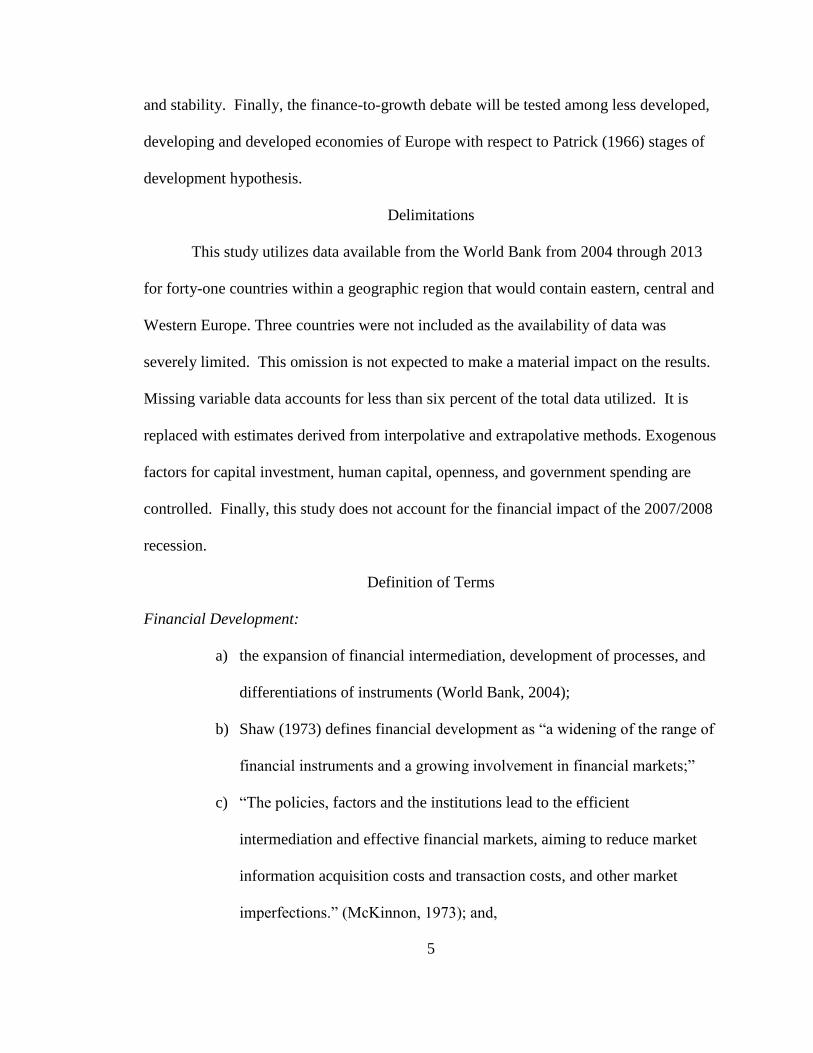
Delimitations
This study utilizes data available from the World Bank from 2004 through 2013
for forty-one countries within a geographic region that would contain eastern, central and
Western Europe. Three countries were not included as the availability of data was
severely limited. This omission is not expected to make a material impact on the results.
Missing variable data accounts for less than six percent of the total data utilized. It is
replaced with estimates derived from interpolative and extrapolative methods. Exogenous
factors for capital investment, human capital, openness, and government spending are
controlled. Finally, this study does not account for the financial impact of the 2007/2008
recession.
Definition of Terms
Financial Development:
a) the expansion of financial intermediation, development of processes, and
differentiations of instruments (World Bank, 2004);
b) Shaw (1973) defines financial development as “a widening of the range of
financial instruments and a growing involvement in financial markets;”
c) “The policies, factors and the institutions lead to the efficient
intermediation and effective financial markets, aiming to reduce market
information acquisition costs and transaction costs, and other market
imperfections.” (McKinnon, 1973); and,
6
d) The costs of acquiring information, enforcing contracts, and making
transactions create incentives for the emergence of particular types of
financial contracts, markets, and intermediaries (Levine, 2005).
Finance Led Growth Theory
Financial development advances economic growth.
Supply-Leading Hypothesis
Financial deepening induces real economic growth.
Demand-Following Hypothesis
Economic growth leads to financial development.
Stages of Development Hypothesis
The stage of economic development determines the direction of causality.
Backwardness Hypothesis
Where countries have more degrees of backwardness, spillover and externalities
have greater effects.
Catchup Hypothesis
The ability or speed of a lesser developed economy to converge with a developing
of developed.
Principal Component Analysis (PCA)
A statistical technique that linearly transforms an original set of variables into a
substantially smaller set of uncorrelated variables that represent most of the information
in the ordinal set of variables (Dunteman, 1989).

7
Components
Clusters of observations as well as outlying and influential observations deduced
from multivariate inter-correlational variables (Dunteman, 1989).
Organization of the Remaining Chapters
Chapter II presents the chronological development of the literature germane to
this dissertation’s hypotheses. The narrative begins with notions dating back to John Law
and Adam Smith and continues with significant contributions from Bagehot, Schumpeter,
Patrick, Goldsmith, and Levine. It covers the development of theory and the
development of methods to test the hypotheses proffered by this research.
Chapter III provides an explanation of the methodology adopted for the
examination of this research’s hypotheses. Following the lead of Griese et al. (2009), the
time series panel data is transformed into principal components and then subjected to
principal component regression. Chapter IV discusses the findings of the principal
component regression and resulting models. Chapter V concludes this research with a
summary and recommendations for further study.

8
CHAPTER II – LITERATURE REVIEW
The literature review is divided into three section: Historical Narrative; Theories
and Hypotheses; and, Empirical Analysis. The Historical Narrative is intended to show
the organized flow of thought as it developed from the earliest discussions to the current
debates. Each successive generation improves upon the research and provides new
questions. The Theories and Hypotheses section provides a more thorough explanation
of the theories that support and the hypotheses that drive the discussion. Finally, the
Empirical Analysis section covers the direction of the hypotheses, researcher tests results,
conflicts between study findings, and statistical testing solutions.
Historical Narrative
The current finance-to-growth debate builds upon a foundation of successive
discussions. The roots of the importance of a financing mechanism find themselves as
far back as John Law and Adam Smith and continued up to Gurley and Shaw in the early
1930s. In the early 1950s counter hypotheses began to be discussed, first with Robinson
(1952) and later refined and defined by Patrick (1966). A third period led by Goldsmith
(1969) and McKinnon (1973) narrowed the focus and began the discussion of the
intermediary roles of markets and banking. The current period includes the introduction
of the endogenous growth theory (Romer, 1986) and empirical analysis by King and
Levine (1993).
Law to Gurley and Shaw
The vast majority of studies begin their finance-to-growth discussion with Walter
Bagehot (1873) or Joseph Schumpeter (1911) but, there is earlier evidence of this
discussion. By deconstruction the institution of banking into banking functions prescribed

9
by Levine (2005) - mobilization of savings (liquidity), evaluation of project viability, and
continuous risk management throughout the life of a project, the discussion can be found
in John Law (1705) and Smith (1776) (De Boyer des Roches, 2013). The functions
Levine list have been a part of banking for centuries in one form or another.
Green (1989) identifies one of these functions, liquidity, with the “real bills
doctrine,” originating in the 17th and 18th centuries. The real bills doctrine asserts that
money can be issued for short term commercial bill of exchange due within the same
production cycle. Output generates its own means of liquidity and banknotes directly
serve the legitimate needs of commerce and trade. John Law in Money and Trade
Considered (1705) proposed that these banknotes could be issued and secured by real
property (Humphrey, 1982). This financing mechanism stimulates manufacturing and
trade, resulting in economic growth (Davis, 1966).
A generation later, Adam Smith in The Wealth of Nations recommended real bills
as a safe commercial bank portfolio asset. Banks in Scotland’s who were considered to
be strong and competitive institutions held these types of notes in their portfolios. The
replacement of specie with paper money like real bills makes his banking theory central
to his theory of economic growth (Laidler, 1981).
Bageot (1873) and Schumpeter (1911) began to formalize the notion that banking
was a significant channel in boosting economic activity. Bagehot (1873) boasted that
“money is economical power … very few are aware how much greater the ready balance
– floating loan fund which can be lent to anyone or for any purpose – is in England.”
Lombard Street fueled the expansion of enterprise in the empire. According to
Schumpeter (1911), as financial intermediaries between savers and borrowers, banks

10
direct surplus capital into investment and investment leads to growth. As agents for
pooled surpluses, resources are reallocated to capital and result in economic growth.
Fisher (1933) explains that creation of debt promotes growth because it allows a
higher rate of return on the use of that debt – investment in capital. Though his article’s
direct point deals with the downside of the overextension of debt, it also stands to reason
that “with ordinary profits and interest, such as through new inventions, new industries,
development of new resources, opening of new lands or new market” economies grow
from the use of debt to fuel this expansion.
Noting a comparative neglect of the financial aspects in the development
discussion, Gurley and Shaw (1955) emphasize the role of financial intermediaries in
improving the efficiency of increasing the supply of loanable funds. Their argument is
based on an observed correlation between economic development and the system of
financial intermediation. Commercial banking is typically the first significant financial
intermediary beyond self-financing through retained earnings. Growth is hindered if
financial intermediaries do not evolve and leaving expansion to be dependent upon self-
financing.
Robinson to Patrick: Contrarian View
Not all economists have agreed with the notion that finance causes growth. A
contrarian opinion asks why do some countries have ineffective financial sectors and
poor economic growth. Joan Robinson (1952) argues that finance development responds
to the growth in demands from the economy. As the economy expands, it requires not
just more of the same financial services, but a broader selection of services. Policy
focused on supplying financial services is misapplied. Direct stimulation of the economy

11
is favored. She is quoted: “where enterprise leads, finance follows.” Other economists
accepted Robinson (1952) and based upon the result of Solow (1956) believed that
financial systems have only minor effects on the rate of investment in physical capital,
and any resulting economic growth (Levine, 1993).
Patrick (1966) followed by providing two terms for the competing hypotheses: the
“supply leading” and the “demand following” relationship between finance and growth.
Supply-leading means that the intentional creation of financial institutions leads to
additional financial products and services which positively affects economic growth.
Demand following postulates that increased demand for financial services occurs because
of economic growth. Patrick (1966) advanced the argument further by proposing a “stage
of development” hypothesis whereby supply-leading financial development can induce
real capital formation in the early stages of economic development … as financial and
economic development proceed, the supply-leading characteristics of financial
development diminish gradually and are eventually dominated by demand-following
development.
Goldsmith-McKinnon-Shaw to Greenwood and Jovanovic
Goldsmith (1968), McKinnon (1973), and Shaw (1973) all stress that the financial
superstructure facilitates the allocation of funds to the best use in the economic system
where the funds yield the highest social return. The quantity and quality of services
provided by this superstructure could partly explain why countries grow at different rates
(King and Levine, 1993).
Goldsmith (1968) makes the case that the separation of the functions of savings
and investment as well as the increasing the range of financial assets increases the

12
efficiency of investment and raises capital formation. This is accomplished through
financial institutions serving as intermediaries, creating products and services for the
pooling and redeployment of capital from savers to borrowers. Financial activities
through these channels increase the rate of economic growth.
McKinnon (1973) investigates the relationship between financial systems
(specifically, domestic capital markets) and economic development. It expanded the
observations to include Argentina, Brazil, Chile, Germany, Korea, Indonesia, and
Taiwan. These case studies strongly suggest that better functioning capital markets,
providing greater liquidity and less friction support economic growth.
Shaw (1973) produces evidence that the health and development of the financial
sector critically matters in economic growth. Monetary systems must have efficiency in
mobilizing savings to induce an increased flow to risk-adjusted loan opportunities
(Moore, 1975). Financial liberalization and deepening stimulate savings and raise rates
of return on investment. Shaw concludes that policies that “deepen” finance stimulate
development (Levine, 2005). The main policy implication of the Goldsmith-McKinnon-
Shaw notion is that government restriction on the banking system (such as interest rate
ceilings, high reserve requirements, and directed credit programs) hinders financial
development and ultimately reduces growth (Khan and Senhadji, 2000).
Financial intermediation promotes growth because it allows for a higher return on
capital. The resulting growth, in turn, provides the additional means to broaden and
deepen financial structures (Greenwood and Jovanovic, 1990). As a result,
intermediation and growth are linked in a continuous development cycle. Freeman
(1986) illustrates how some industries or sectors of the economy have very large capital

13
requirements and thus necessitate the pooling of funds from many different sources.
Financial intermediaries perform this pooling task. This is demonstrated in the direct
customer relationship of the deposit and loan functions of commercial banks as well as in
the indirect connection provided by the stock, bond and futures markets. Regulations,
limits or interference by regulatory authorities on intermediaries, inherently restrict the
finance-to-growth dynamic.
Romer-Lucas-Rebelo to Levine
The Romer (1986), Lucas (1988), and Rebelo (1991) contribution to the body of
knowledge is in the endogenous process of the growth model, where it does not depend
on exogenous technological change. They focus on two channels through which each
financial function may affect economic growth – capital accumulation and innovation.
The financial system affects capital accumulation either by altering the savings rate or by
reallocating savings among different capital producing technologies. Innovation focuses
on the invention of new production processes and goods. Intermediation facilitates
modernization capital and improvement of labor (Romer 1990 and Aghion and Howitt,
1992). The latter is a broader interpretation of "capital" that includes human capital.
Development of human capital (labor) is a driving force behind economic growth
(Grossman and Helpman, 1991). Human capital’s importance is in its ability to overcome
the steady state.
King and Levine (1993) is one of the first to empirically define financial
development using four indicators, each designed to measure some aspect of the financial
services sector. These determinants include: a) the ratio of liquid liabilities to GDP; b)
the ratio of credit issued to nonfinancial private firms to total credit extended; c) the ratio

14
of credit issued to nonfinancial private firms to GDP; and d) distinguishing between
central bank and private bank functions as well as size of intermediaries. King and
Levine’s use of these variables provides a more complete picture of financial
development than a single measure.
Researchers have developed rigorous theories of the evolution of the financial
structures and how the mixture of markets and banks influences economic growth:
Patrick (1966), Merton and Bodie (1995), and Levine (2005) for example. Some
theories stress the advantages of market-based systems, especially in the promotion of
innovative and more R&D based industries (Allen, 1993), while others emphasize how
commercial banking exerts a positive discipline and governance over corporate structure
(Levine, 1999) and (Arestis and Demetriades, 1997). Financial instruments, markets,
and institutions arise to mitigate the effects of information and transaction costs (Levine,
1997).
More recent models separate and test the benefits derived from the bank and
securities markets influences (Arestis and Demetriades (1997), Greenwood and Smith
(1997), and Levine (2002)). Within the financial development discussion, there is some
debate over the contribution of commercial banking versus markets. Arestis and
Demetriades (1997) finds “the effects of banks are more powerful … suggest that the
contribution of stock markets on economic growth may have been exaggerated.”
Banking is a primary, first contact intermediary, necessary for early stimulation of
growth. Greenwood and Smith (1996) investigate the specific markets to growth and
growth to markets discussion and sides with markets providing efficient channeling of
investment capital for large capital investments. Levine (2002) in a broad cross-country

15
review determines that there is no evidence that one channel (markets or banking) is
superior to the other. Among lesser developed countries Tadesse (2002) finds that the
banking channel outperforms the securities market in its effects on economic growth.
This lends support to Patrick’s (1966) stages of growth hypothesis, that the banking
channel is more effectual than the other channels in lesser developed economies. Levine
(2005) summarizes that the body of literature suggests that where there are countries with
better functioning banks and market, the countries grow faster.
According to King and Levine (1993), better financial services expand the scope
and improve the efficiency of factors of growth. This leads to an acceleration of
economic growth. In contrast, policies that repress financial development, impede
innovative activity and slows economic growth. This is due to reduced services provided
by the financial system to savers, entrepreneurs, and producers.
According to Merton and Bodie (1995, p.12) “In a rising to ameliorate transaction
and information costs, financial systems serve one primary function: they facilitate the
allocation of resources, across space and time, in an uncertain environment.” Levine
(2005) states that financial intermediaries work principally to improve:
a) Acquisition of information on firms;
b) Intensity with which creditors may exert corporate control; and
c) Provide risk-reducing arrangements, the pooling of capital, and ease of
making transactions.
Naghshpour (2013) proffers that banks: serve as a more efficient intermediary
between borrower and savers; collecting, processing and evaluating information;
reducing moral hazard; improving the ease and speed of transactions through the creation

16
of money and decreasing frictions; and, innovating new financial products that create
additional opportunities for the transfer of capital.
Theory
Theory suggests that financial institutions, their instruments, and resulting
markets occur to mitigate the effects of information (asymmetric) and transaction cost
(friction). To the degree they are successful, savings rates and investment decisions are
influenced. This section discusses the theoretical foundation for the banking-to-growth
nexus and its particular explanation for more rapid growth in the emerging economies of
Eastern and Central Europe. The discussion is comprised of four parts:
a) Relevance of the endogenous growth theory;
b) Financial development’s impact on resource allocation decisions and
savings rates;
c) Financial development theory; and,
d) Effects of convergence, spillover, and backwardness.
Figure 1 below demonstrates the mapping of the theoretical foundation for the discussion
in this research.

17
Theories and Hypotheses
The neoclassical theory (Solow-Swan model) states that with a proper mix of
labor, capital, and technology economic growth will result. By varying the amounts of
labor and capital in the production process, an equilibrium state can be accomplished.
When innovation occurs, labor and capital adjust to achieve a new equilibrium. Perhaps
the elevation of innovation in the endogenous growth model better explain the
relationship between financial development and economic growth.
Endogenous Growth Theory
Numerous researchers propose that the endogenous growth model demonstrates
that growth is related to financial development. King and Levine (1993) suggests
innovation is the key engine of growth. When financial institutions evaluate innovative
projects, provides the intermediation between savers and borrowers, and monitors the
project going forward, they affect growth. Productivity may be demonstrated in
increased human capital, increased capital efficiencies, and underwriting breakthrough
Endogenous Growth Theory
Convergence
Spill-over
Catch-up
Backwardness
Resource Allocation
Savings Rates
Financial Development
Financial Institutions Theory
Banking and Market Theory

18
innovations. Well-functioning financial markets improve productivity which affects
growth (Demetriades and Hussein, 1996).
Resource Allocation Decisions
Levine (2005) stresses that the theoretical argument for a finance-to-growth
causality should focus on finance’s influence on resource allocation. Resource
allocations do not occur in a vacuum or with randomness, rather they are influenced. The
link between finance and resource allocations can be established by understanding the
functions of finance and its effects.
Financial markets influence growth through resource allocation efficiencies
(Greenwood and Jovanovic, 1990). Without financial markets, individuals would have
far less access to information to consider liquidity, risk and return. Levine (1991) and
Bencivenga and Smith (1991) each propose models that identify channels (markets,
banking, insurance, and FDI) through which financial markets provide access to that
information. Resource allocation decisions can be reinforced, altered, and rechanneled
with improved information sourced from finance.
In a market economy information is valued in order to channel resources to their
highest and best use. Financial institutions as intermediaries, find it necessary to
assimilate, process and disseminate information. This could occur as an entrepreneurial
enterprise or as a necessity to decrease risk and or raise return. If the lack of information
or the cost of developing information provides too strong a “friction” then resource
allocation is negatively affected. Boyd and Prescott (1986) suggests intermediaries
relieve individual investors of the significant fixed cost associated with information. The
cost of information is typically too expensive for an individual investor. Financial

19
institutions and ancillary business can source information to the private sector at a much
less cost. This is a reduction of friction and an inhibitor in resource allocation. Levine
(2005) references Greenwood and Jovanovic (1990), “Assuming that entrepreneurs solicit
capital and that capital is scarce, financial intermediaries that produce better information
on firms will thereby fund more promising firms and induce a more efficient allocation of
capital” (p. 871).
Savings Rates
Increasing and decreasing returns affect savings rate and invoke possibilities of
consumer choice theory. Income and substitution effects are considered. As
intermediaries provide services that result in lower risk and improved resource allocation
savings rates may actually decrease. Financial development may negatively affect
savings rates. Referencing Levhari and Srinivasan (1969), Levine (2005) concludes that
the financial products and services that banks provide which leads to lower risk and
improved resource allocation results in lower savings rates.
Financial Development
According to the Word Bank (2003), financial development means the
improvement of the financial sector. More recently it has been defined in terms of
improvement in access, depth, efficiency, and solvency. It can also be discussed in terms
of benefits and functions.
McKinnon (1973) lists two significant benefits derived from liberalization of
financial markets:
a) increased intermediation between savers and investors, and
b) the efficient flow of resources among people and institutions over time.

20
With less constraints, savings is encouraged and capital accumulation follows.
Furthermore, efficiency in the transferring of capital from less productive to more
productive sectors occurs. “The efficiency, as well as the level of investment, is thus
expected to rise with the financial development that liberalization promotes” (McKinnon,
1973).
Fitzgerald (2007) further describes financial development by offering five broad
functions financial systems provide:
1. Produce information ex ante about investments;
2. Mobilize and pool savings and allocate capital;
3. Monitor investments and exert corporate governance after providing finance;
4. They facilitate the trading, diversification, and management of risk; and
5. To ease the exchange of goods and services.
Information is a key function provided by financial institutions. Ex ante
information regarding investment provides the basis for expectation. Financial
institutions in general and commercial banks specifically create produce ex ante
information to be shared with clients and the market.
The needs of many capital investments require significant financial backing.
Financial institutions mobilize and pool savings from large number of savers, thus
allowing the allocation of capital toward those projects. Patrick (1966) uses the
development of railroad in the United States as an example of a project of such
magnitude that it creates the necessity of a bond market to finance a project.
Intermediation is a continuous process requiring regular monitoring of the capital
investment. Financial institutions exercise that monitoring through corporate governance

21
after providing financing (LaPorta et al., 2000). The general welfare of the asset, asset
class, and the financial system are secured with the continuous oversight and
accountability.
Financial institutions measure and manage risk. Products and services within the
industry efficiently transfer risk from one institution to another that is best able to bear
that risk for a price. The creation of the trading opportunity and the counterparty willing
to accept the risk is a significant function financial development affords for risk
management (Hauner, 2009).
Finally, financial institutions create mechanisms that decreases the friction in the
exchange of goods and services. Levine (1997) states “liquidity is the ease and speed
with which agents can convert assets into purchasing power.” Financial institutions add
to the ease and speed by decreasing the friction – the time and effort that may be
obstacles.
Financial Development and Growth
The simplest expression of the endogenous growth model (known as the AK
model) is shown as Yt = A Kt L where output is a function of capital stock.
According to Pagano (1993) financial development positively affects growth in three
ways:
a) Raising the proportion of savings directed to investment;
b) Increases the social marginal productivity of capital; and,
c) May positively influences the private savings rate.
Leakage is a problem when transforming savings into investment. This occurs in
loan spreads, fees regulations, taxation, and inefficiencies. If development occurs, the

22
leakage is decreased and the growth rate increases. This raises the proportion of savings
directed to investment.
Risk adverse individuals will frequently forgo longer commitment investments
which may be more productive but are also less liquid. Intermediaries (banks) can reduce
this inefficiency by satisfying the liquidity risk of depositors and investing in longer-
term, illiquid, and higher yielding projects. This is facilitated by asset/liability
management practices by the intermediary, only maintaining a level of liquidity
necessary to meet the actual aggregated needs of the depositors. This raises the
productivity of capital.
Private savings rates may increase and in some cases decrease under different
financial development dynamics. Higher liquidity and multiple risk diversification
systems decrease the margin between borrowing and savings rates. According to Pagano
(1993) development may reach such levels of sophistication and efficiency that savings
rates decline.
Financial Institutions Theory
According to Allen and Gale (2000), financial systems are crucial for the
allocation of resources in an economy. As intermediaries in the financial system,
financial institutions channel the savings they receive from households to the corporate
sector. The core of their intermediary role has been based upon reducing the friction of
transaction cost and development asymmetric information. With the added complexity of
products and market participants, Allen and Santomero (1997) offer additional roles – a)
facilitators of risk transfer, and b) reducing participation costs.

23
Financial futures and options markets are examples of risk management. These
risk management tools are typically shared between intermediaries instead of households
and corporate firms. Other sectors desiring to participate in these products and markets
may find the cost prohibitive. Financial institutions can be the gateway through reduced
participation costs. While the former intermediary roles have decreased, these new
purposes are increasing in importance as well as complexity (Allen and Santomero,
1997).
Banking vs Market-Based Theory
Within the finance-to-growth discussion, there is debate over the comparative
importance of bank or market channels. The primary research in this area is in Allen and
Gale (2000), Levine (2000), and Demirguc-Kunt and Levine (2001).
Allen and Gale (2000) discuss the merits of the bank-based vs market-based
systems debate. They posit that it is an argument between two different perspectives –
development economics and corporate finance. Development economics theory focuses
on banks which take in deposits from savers and make loans to borrower. Corporate
finance theory is directed at debt and equity issued by firms.
Levine (1999) offers a reconciling notion that the two are part on one discussion –
financial services. The choice is not between banks or markets, but rather an
environment whereby the particularly effective services are available at particular stages
of economic development. In the earlier stages of development, economies may rely
more on bank-based systems. Banks are first stage growth intermediaries. As the
economies become more developed, market-based systems that depend upon well-
functioning securities markets become more important. Market-based systems are
24
second stage intermediaries and promote long-run economic growth (Demirguc-Kunt and
Levine, 2001).
Convergence Theory
The convergence theory is a notion that all economies should eventually become
equal (converge) in terms of per capita income. Poorer countries will tend to grow at a
faster rate than their richer counterparts. This is attributable to two reasons: (a) poorer
countries can enjoy innovation and technologies by duplication, and (b) developing
countries are not burdened by diminishing returns to capital as the developed.
Easterly and Levine (2001) explains how this may be directly applied to financial
development and growth. It adds an additional qualifier. Convergence is incumbent
upon some threshold level of financial development. Those economies above this
threshold will all converge to the long-run growth rate, while those below will have lower
rates.
Spillover
The spillover or replication of financial depth from more developed economies
may spur economic growth in less developed countries. Yet, the contribution may
strongly depend on the circumstances in the recipient countries (Guiso, Sapienza, and
Zingales, 2004). Chirot (1989) proposes that there are reasons for the problems of
centuries of slow growth and a long history of economic backwardness. It points to
Eastern Europe in contrast to Central Europe where the former was distant from the west,
agriculturally based and had a significant history of elite rule. Central Europe enjoyed
the spillovers from Western Europe because of proximity, but also because the political
structure was more open to development.

25
Catchup Effect
The catch-up effect is that part of the convergence theory explaining why lesser
developed nations may grow faster than developed. The reasoning for this phenomenon
is primarily attributed to access to technology and innovation from nearby advanced
economies. This access allows lesser developed nations to immediately adopt economies
and efficiencies without sinking significant investment in transitioning capital.
It is necessary to state that this effect has not been universally successful. Many
developing economies have failed to see substantial improvements, or at least growth
rates comparable to the developed. Other factors that similarly influence growth like
social, institutional or political differences are thought to limit or suppress growth.
Acemoglu and Robinson (2006) offers a model where institutional development is
blocked by political elites. The heart of this theory is that political elites resist change
and innovation promote change.
Backwardness
“Backwardness” is a consideration in the distinction of varying growth rates.
Gerschenkron, (1952) proposes that where countries have greater degrees of
backwardness, spillover and externalities have greater effects. This is in contrast
developed economies where there is less marginal benefits. Technological and
informational spillovers can have an immediate effect without the cost of development.

26
Empirical Analysis
This section is organized as a summary of the econometric approaches used in the
literature that investigate the finance-to-growth discussion. Levine (2005) attributes the
first empirical analysis to Goldsmith (1968). Goldsmith gathered data from thirty-five
countries for the period 1860 to 1963 and correlated the size of financial intermediaries
with the quality of the financial functions they provide. From this research, Goldsmith
acknowledged a series of shortcomings that later studies should investigate – primarily
further attribution to financial development, more countries, longer time series, additional
controls, and focus on predictability. His list of shortcomings provides a framework to
catalog the follow-up research. This section is divided into a) Case studies, b) Panel data,
c) Time-series, and d) Principal component Analysis.
Case Studies
Case studies by Cameron et al. (1967) and McKinnon (1973) provide the first
measured discussions of the relationship between financial development and growth.
Though lacking statistical analysis, the cases are able to provide observations regarding
the interactions of the political, regulatory, administrative, industrial and financial
structures. These two studies document the relationship of financial intermediaries,
markets, and government intervention during periods of industrialization: e.g. England
1750 -1844; France 1800 – 1870; Germany 1815 – 1870; and, Japan 1868 – 1914. From
the country case studies, Cameron et al. (1967) concludes that banking plays a positive,
growth causing role. Similarly, McKinnon (1973) deduces that developed financial
systems stimulate economic growth.
27
Haber (1991) also uses the case study approach. His study uses firm-level data
for Brazil, Mexico, and the United States and infers that the development of capital
markets leads to both industrial composition and economic growth. Liberalization of
policies and restrictions on Brazilian and Mexican financial markets in the late 19th
century led to growth. Comparisons between Brazil and Mexico highlight that
differences in financial development can have a significant impact on the rate of
economic growth.
On a micro and firm level basis, other researchers like Guiso et al. (2002) find
financial development enhances business start-ups and fosters industrial competition in
Italy. Cull and Xu (2005) observes the advantage of private ownership over public in
encouraging retaining earnings. Bertrand et al. (2007) examines the financial deregulation
of the 1980s and the positive impact on competition in the credit markets.
These examples illustrate the theses developed for countries, sectors, and markets
regarding financial development and describe certain observed behaviors. While these
studies simplify aspects of the finance-to-growth notion, their conclusions may not be
fairly generalized.
The next two sections are organized around econometric approaches that measure
and examine the finance-to-growth relationship.
Panel Data
King and Levine (1993)
King and Levine (1993) takes Goldsmith’s research and increases the number of
countries to 77 for a thirty year period from 1960 to 1989. They also for the first time
specified financial development with three independent variables that measure:

28
a) Size of the intermediaries;
b) Degrees to which bank credit is made available to all parties, public and
private; and
c) Credit to private enterprises.
In the regression, they controlled for other factors associated with economic growth –
income, education, exchange rates, trade, fiscal and monetary policy. Their results are
limited to illustrating the effects of changes in financial (primarily banking) development
and long term growth and not the causes.
Levine and Zervos (1998)
As King and Levine (1993) expanded the banking channel measurements, Levine
and Zervos (1998) attended to the construction of numerous measures of stock market
development. To assess the relationship between stock market development and growth,
they sample 42 countries over the period 1976 – 1993. Their results indicate that the
level of market liquidity (turnover) with banking development (size of assets and
deposits) are significantly correlated with economic growth. Similarly to King and
Levine (1993), this research does not address the issue of causality.
Loayza and Ranciere (2002)
This paper attempts to reconcile the apparent `contradiction between the supply-
leading and the demand-following hypotheses. Loayza and Ranciere (2002) use an
empirical explanation of the apparently opposing effects of financial intermediation.
Employing Pesaran’s Pooled Mean Group Estimator (PMG), the analysis demonstrates a
positive long-run relationship between finance and growth. There is also evidence that a
negative short-run relationship exist. This analysis reflects the ‘stages of growth’ notion
29
posited by Patrick (1966). The significant contribution to the literature is the
identification of causality.
Rioja and Valev (2004)
The impact of financial development varies in the way it affects productivity and
capital accumulation in developed, developing and less developed economies. Rioja and
Valev (2004) test this using the Generalized Method of Moments regression (GMM) for
74 countries. Their results confirm the hypothesis – finance has a strong positive impact
on productivity in developed countries while finance affects capital accumulation in less
developed economies.
Beck and Levine (2004)
This research reviews the impact of two financial channels, markets, and banking,
on economic growth. The study uses panel data for the period 1976-98, and like Rioja
and Valev (2004), applies GMM techniques. The results indicate that markets and banks
positively affect economic growth.
Time Series
Concurrent with the use of panel data is the substantial use of time-series. Time
series studies frequently use Granger causality test and vector auto-regression (VAR)
procedures to determine the direction of causality. Arestis and Demetriades (1997),
Neusser and Kugler (1998), Xu (2000), and Christopoulos and Tsionas (2004) are the
most notable studies utilizing time series.
Arestis and Demetriades (1997)
Arestis and Demetriades (1997) time-series focuses on measures of both markets
and banking in their finance-to-growth investigation. The results indicate that the effects
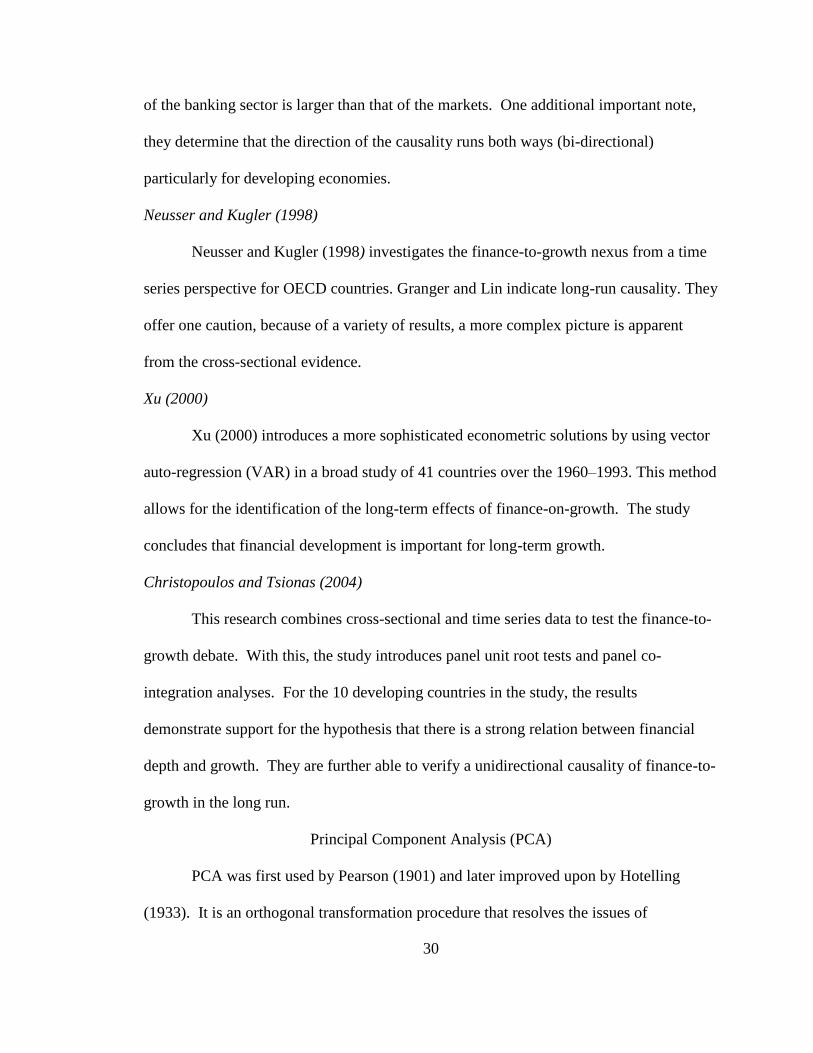
30
of the banking sector is larger than that of the markets. One additional important note,
they determine that the direction of the causality runs both ways (bi-directional)
particularly for developing economies.
Neusser and Kugler (1998)
Neusser and Kugler (1998) investigates the finance-to-growth nexus from a time
series perspective for OECD countries. Granger and Lin indicate long-run causality. They
offer one caution, because of a variety of results, a more complex picture is apparent
from the cross-sectional evidence.
Xu (2000)
Xu (2000) introduces a more sophisticated econometric solutions by using vector
auto-regression (VAR) in a broad study of 41 countries over the 1960–1993. This method
allows for the identification of the long-term effects of finance-on-growth. The study
concludes that financial development is important for long-term growth.
Christopoulos and Tsionas (2004)
This research combines cross-sectional and time series data to test the finance-to-
growth debate. With this, the study introduces panel unit root tests and panel co-
integration analyses. For the 10 developing countries in the study, the results
demonstrate support for the hypothesis that there is a strong relation between financial
depth and growth. They are further able to verify a unidirectional causality of finance-to-
growth in the long run.
Principal Component Analysis (PCA)
PCA was first used by Pearson (1901) and later improved upon by Hotelling
(1933). It is an orthogonal transformation procedure that resolves the issues of
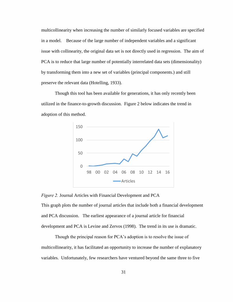
31
multicollinearity when increasing the number of similarly focused variables are specified
in a model. Because of the large number of independent variables and a significant
issue with collinearity, the original data set is not directly used in regression. The aim of
PCA is to reduce that large number of potentially interrelated data sets (dimensionality)
by transforming them into a new set of variables (principal components.) and still
preserve the relevant data (Hotelling, 1933).
Though this tool has been available for generations, it has only recently been
utilized in the finance-to-growth discussion. Figure 2 below indicates the trend in
adoption of this method.
Journal Articles with Financial Development and PCA
This graph plots the number of journal articles that include both a financial development
and PCA discussion. The earliest appearance of a journal article for financial
development and PCA is Levine and Zervos (1998). The trend in its use is dramatic.
Though the principal reason for PCA’s adoption is to resolve the issue of
multicollinearity, it has facilitated an opportunity to increase the number of explanatory
variables. Unfortunately, few researchers have ventured beyond the same three to five
0
50
100
150
98 00 02 04 06 08 10 12 14 16
Articles

32
proxies most used in the literature. One exception is Lipovina-Bozovic et al. (2016)
where in his research the study utilized nine independent variables. As the description
and measurement of financial development is broadened and deepened and the data
collection for those measurements expands, PCA’s contribution should not only be
recognized in its solution for multicollinearity, but also in its greatest strength –
uncovering important underlying structures in the data.
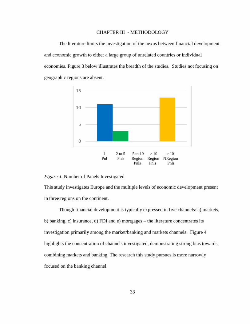
33
CHAPTER III - METHODOLOGY
The literature limits the investigation of the nexus between financial development
and economic growth to either a large group of unrelated countries or individual
economies. Figure 3 below illustrates the breadth of the studies. Studies not focusing on
geographic regions are absent.
Number of Panels Investigated
This study investigates Europe and the multiple levels of economic development present
in three regions on the continent.
Though financial development is typically expressed in five channels: a) markets,
b) banking, c) insurance, d) FDI and e) mortgages – the literature concentrates its
investigation primarily among the market/banking and markets channels. Figure 4
highlights the concentration of channels investigated, demonstrating strong bias towards
combining markets and banking. The research this study pursues is more narrowly
focused on the banking channel
0
5
10
15
1 2 to 5 5 to 10 > 10 > 10
Pnl Pnls Region Region NRegion
Pnls Pnls Pnls
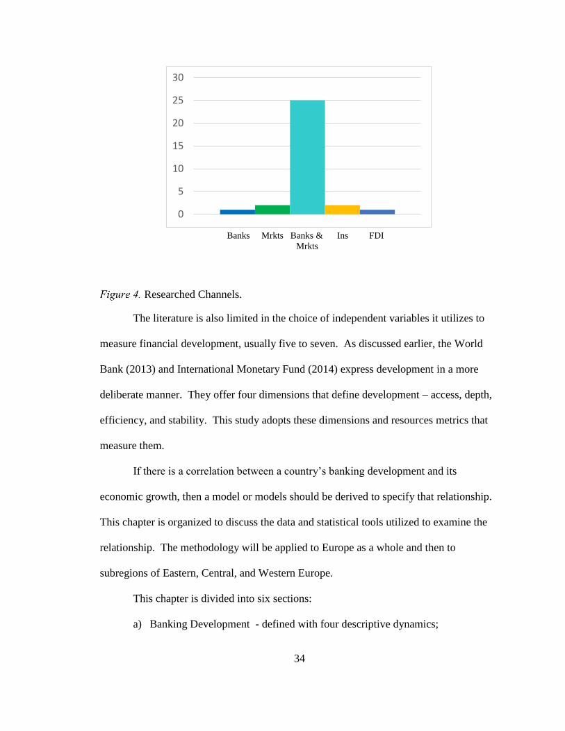
34
Researched Channels.
The literature is also limited in the choice of independent variables it utilizes to
measure financial development, usually five to seven. As discussed earlier, the World
Bank (2013) and International Monetary Fund (2014) express development in a more
deliberate manner. They offer four dimensions that define development – access, depth,
efficiency, and stability. This study adopts these dimensions and resources metrics that
measure them.
If there is a correlation between a country’s banking development and its
economic growth, then a model or models should be derived to specify that relationship.
This chapter is organized to discuss the data and statistical tools utilized to examine the
relationship. The methodology will be applied to Europe as a whole and then to
subregions of Eastern, Central, and Western Europe.
This chapter is divided into six sections:
a) Banking Development - defined with four descriptive dynamics;
0
5
10
15
20
25
30
Banks Mrkts Banks & Ins FDI
Mrkts

35
b) Data - reasons for the selection and use in the statistical analysis;
c) Statistical test - normality, collinearity, and stationarity;
d) Principal Component Analysis;
e) Principal Component Regression; and,
f) Model specification.
Banking Development
Development is vague in both its description and measurement. The largest body
of literature depends upon a few readily available metrics to represent financial
development. The World Bank (2004) first introduce a concept of four dimensions to
describe and measure financial development. These dimensions are access, depth,
efficiency, and solvency. Access and depth provide an external connection between
banking institutions and their customers. Efficiency and stability reflect the internalized
structure and organization of the institutions themselves. This study utilizes the
foundation of four dimensions in its qualification of banking development.
With each dimension, multiple metrics measuring banking attributes and
functions are selected. These metrics provide overlapping explanations. This certainly
can lead to collinearity, but this issue will be dealt with later in this chapter. With the
problem of collinearity, a significantly larger database of metrics is available and thus
improved specification of the models.
Data
The principal source of data for this study is the World Bank’s Data Base 2015.
The database contains as many as four hundred metrics on up to two hundred and six
countries. There are currently seventy-eight financial metrics. This study is utilizing 21

36
independent variables, 4 control variables, and 1 dependent variable in the data set. The
data set is structured as panel data for thirty-eight countries over a ten year period from
2004 to 2013.
Countries
Forty-one countries spanning the European continent are subdivided into three
geographic and economic regions: Eastern Europe, Central Europe, and Western Europe.
The geographic divisions largely overlap the levels of economic development. As
presented earlier in this study, the countries’ level of economic development increases as
they range from east to west. The methodology begins with fifteen countries in Eastern
Europe, seven countries in Central Europe, and nineteen countries of Western Europe.
Table 1 below lists the countries in the studies data set.
Table 1
Listing of Countries in the Database
Eastern Europe Central Europe Western Europe
Albania Serbia Czech Republic Austria Luxembourg
Armenia Slovenia Estonia Belgium Malta
Belarus Turkey Hungary Cyprus Netherlands
Bosnia Ukraine Latvia Denmark Norway
Bulgaria Lithuania Finland Portugal
Croatia Poland France Spain
Kosovo Slovakia Germany Sweden
Macedonia Greece Switzerland
Moldova Ireland U K
Romania Italy
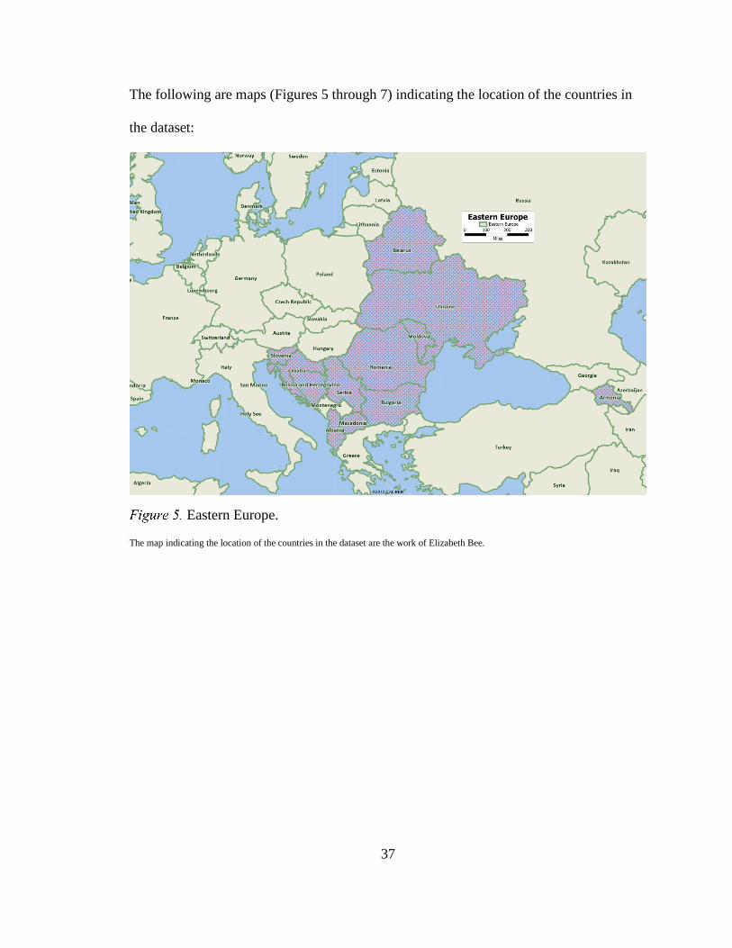
37
The following are maps (Figures 5 through 7) indicating the location of the countries in
the dataset:
Eastern Europe.
The map indicating the location of the countries in the dataset are the work of Elizabeth Bee.
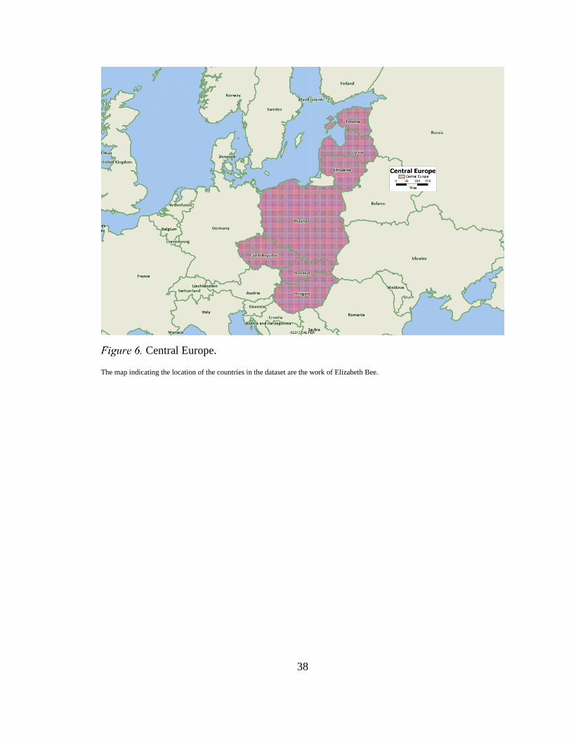
38
Central Europe.
The map indicating the location of the countries in the dataset are the work of Elizabeth Bee.
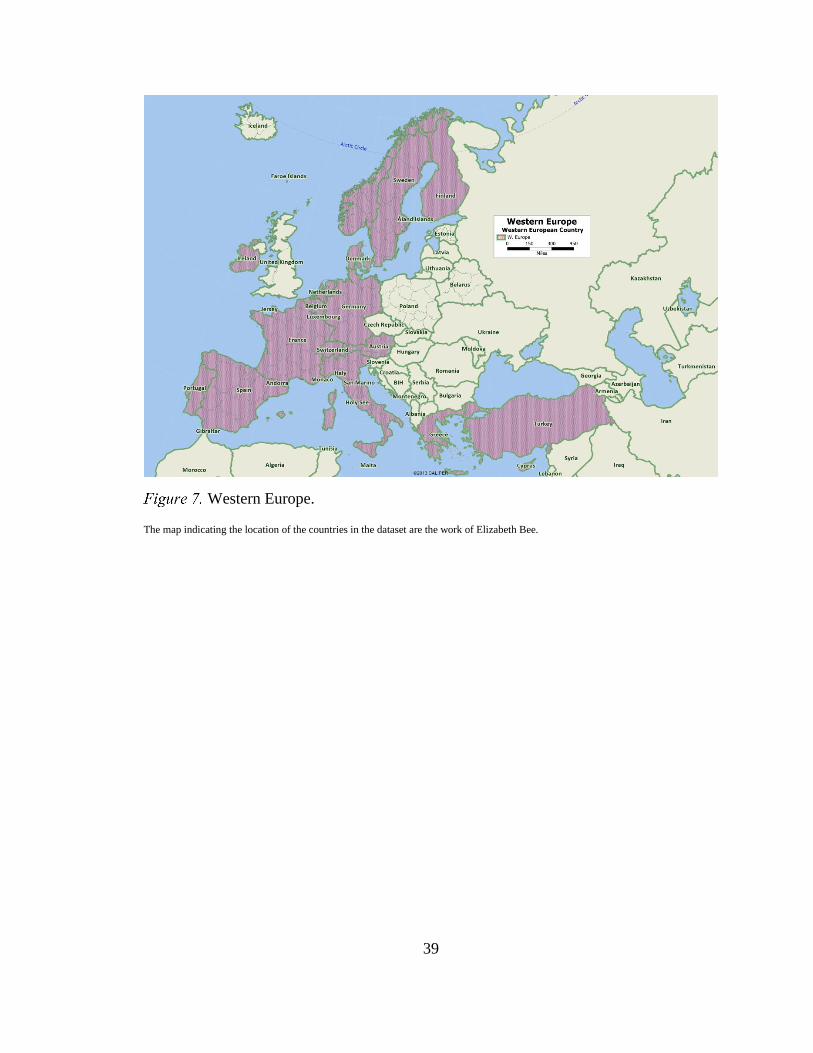
39
Western Europe.
The map indicating the location of the countries in the dataset are the work of Elizabeth Bee.

40
Economic Growth
Following the convention most utilized in the literature, this study adopts the rate
of the change in growth of gross domestic product as its measurement for the dependent
variable.
Banking Development Independent Variables
The richness of the World Bank and International Monetary Fund’s Global
Financial Development database allows for a large number of metrics to be utilized as
independent variables. Thirty-one banking metrics are available, twenty-two are selected
due to the number of countries participating and the depth of years reported. Each of
these variables represents one of four dimensions – access (6), depth (6), efficiency (4),
and stability (6).
Access. The degree to which individuals can and do use banking services.
• ATMs 100,000 adults
• ATMs per 1,000 KM2
• 5 Bank asset concentration
• Bank branch per 100,000 adults
• Bank branch per 1,000 KM2
• Bank concentration
Depth. The size of banking institutions’ components.
• Bank deposits to GDP
• Domestic credit to private sector to GDP
• Deposit money bank assets to deposit money assets
• Deposit money banks’ assets to GDP

41
• Liquid liabilities to GDP
• Private credit by deposit money banks to GDP
Efficiency. The measurement of the management of productivity and
performance.
• Bank cost to income
• Noninterest income to total income
• Overhead costs to total assets
• Return on assets
Stability. The financial and capital stability of the banking industry.
• Capital to assets ratio
• Regulator capital to risk- weighted assets
• Credit to deposits
• Net interest margin
• Non-performing loans
• Return on Equity
Control Variables
In order to examine the effect of banking development on economic growth, this
research utilizes four control variables most often utilized in the literature. These
variables allow us to analyze the true impact of banking on growth as we control for
possible influential effects. The control variables used in this paper include capital
investment, human capital, openness, and government spending. The data is available
from the World Bank.

42
Capital Investment. Apergis et al. (2007) suggests two points of value for
investment – a) an increase in investment results in growth and b) spillover effects and
economies of scale result in growth. Christopoulos and Tsionas (2004) found investment
to have a positive effect and is statistically significant. The studies have focused on
Gross Capital Investment as the singular proxy.
Human Capital. Lucas (1993) finds that higher levels of education creates an
ability for a country to absorb new technologies and become innovative. Enjoying
spillover and applying new information are better suited for more educated populations.
Human capital influences the growth of total factor productivity and does so by attracting
physical capital (Benhabib and Spiegel, 1994). The percent of population with secondary
education is the most frequently used proxy.
Openness. Trade appears to raise income by spurring the accumulation of physical
and human capital. (Barro and Sala-i-Martin, 2004 and Frankel and Romer, 1999). Trade
creates interactions in exchange of ideas, specialization, and dissemination of knowledge
– all resulting in greater growth. The literature utilizes Net Exports for the proxy for
openness.
Government Spending. According to Barro and Sala-i-Martin (1995), government
expenditures on education and infrastructure promotes growth. Similarly, Easterly and
Rebelo (1993) review fiscal policy correlations and conclude that investment in transport
and communication is robust with respect to growth. In lieu of deconstructed
components, this study will use aggregate Expenditures.

43
Statistical Tests
The data is checked for normality, collinearity, and stationarity.
Normality
The assumption of normality for the sample distribution is tested. The three
default test in Stata 12 are:
a) Doornick-Hansen, b) Shapiro-Wilk, and, c) SKtest.
The Doornik-Hansen test for multivariate normality is based on the skewness and
kurtosis of multivariate data (Doornik and Hansen, 2008). Shapiro-Wilk and SKtest are
two other general tests designed to detect departures from normality. All three tests are
comparable in power.
Collinearity
In multiple regression, an event can arise when two or more independent variables
are highly correlated. The collinear variables essentially share the same information
about the dependent variable and are redundant. According to Wooldridge (2010), the
principal danger of such data redundancy is the overfitting in regression models.
Stationarity
A time series is stationary if a shift in one time period to the next doesn’t cause a
change in the shape of the distribution. Since the data in this study is structured in time
series, there is concern for non-stationarity. As a result, some stochastic processes (unit
root) may cause a problem with statistical inference. Its presence can cause spurious
regressions or errant predictions due to invalid assumptions (Granger and Newbold,
1974). A test is necessary to determine the presence of unit root. The Levin-Lin-Chu test
(LLC) is utilized for the four control variables and twenty-two independent variables.

44
This study adopts Cihak et al. (2012) use of the World Bank dimensionalities.
The PCA method provides components derived from variables measuring those four
dimensions to characterize banking development. The result is a single model expressing
all the component(s) without the burden of collinearity.
Principal Component Analysis
Because of the large number of independent variables and a significant issue with
collinearity, the original data set is not directly used in regression. The aim of PCA is to
reduce that large number of potentially interrelated data sets (dimensionality) by
transforming them into a new set of variables (principal components.) and still preserve
the relevant data (Hotelling, 1933). The method defines a set of principal components
with the direction having the greatest variability in the data (Lavrenko, 2015). The value
is that these principal components (PCs) are uncorrelated and retain most of the original
group’s variation.
The process deconstructs the data set into eigenvalues (magnitude), from which
eigenvectors (direction) are constructed. The eigenvectors with the highest eigenvalues
are the principal components. In this study, there are twelve independent variables
measuring the four general aspects of financial development. It is the intention of this
study to utilize PCA to re-expresses a data set into its most meaningful basis. This new
basis has filtered out all the noise that disguises the relationships and exposes the
underlying structure (Shlens, 2014).
Following Gries, Kraft, and Mejerrieks (2009), this study uses PCA to transform
the independent variables into principal components. Qualified components are used in
the regression sequence. To transform the data and select the appropriate components
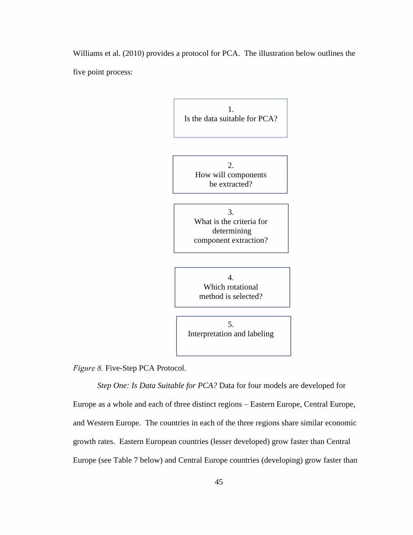
45
Williams et al. (2010) provides a protocol for PCA. The illustration below outlines the
five point process:
1.
Is the data suitable for PCA?
2.
How will components
be extracted?
3.
What is the criteria for
determining
component extraction?
4.
Which rotational
method is selected?
5.
Interpretation and labeling
Five-Step PCA Protocol.
Step One: Is Data Suitable for PCA? Data for four models are developed for
Europe as a whole and each of three distinct regions – Eastern Europe, Central Europe,
and Western Europe. The countries in each of the three regions share similar economic
growth rates. Eastern European countries (lesser developed) grow faster than Central
Europe (see Table 7 below) and Central Europe countries (developing) grow faster than

46
Western Europe (developed.) PCA necessarily requires the data to be collinear. As a
result, the data should to be tested for suitability. According to William et al. (2010) and
Katchova (2013), the Kaiser-Meyer-Olkin (KMO) measure is the recommended test. The
KMO test measures that suitability by providing the proportion of variance which might
be caused by underlying factors
Step Two: How Components Will Be Extracted. Four sets of principal component
are derived from the orthogonal transformation of twenty-two independent variables.
Each set relates to the specific relationships within the European, Eastern, Central, and
Western European economies.
Step Three: What is the Criteria for Determining Component Extraction? The
goal is to reduce the twenty-two independent variables into a lesser number of
components yet maintain a significant amount of the information in the variation. Several
criteria are available to determine an optimal number. According to Williams et al.
(2010), multiple approaches are preferable and two of the most often used are the Kaiser
Rule and the Scree test.
Step Four: Selection of Rotational Method. Rotation produces a more
interpretable solution by maximizing high item loadings (correlations of the independent
variables) and minimizing the low item loadings. Two methods are typically utilized:
Varimax (orthogonal) and Promax (oblique). Varimax rotation first developed by Kaiser
(1958) is the most common rotational technique. While this research uses both,
interpretation is based on the Varimax rotations.
Step Five: Interpretation and Labeling. A singular loading or set of loadings may
be identified as a result of the rotation as having a particular theme or weight. These
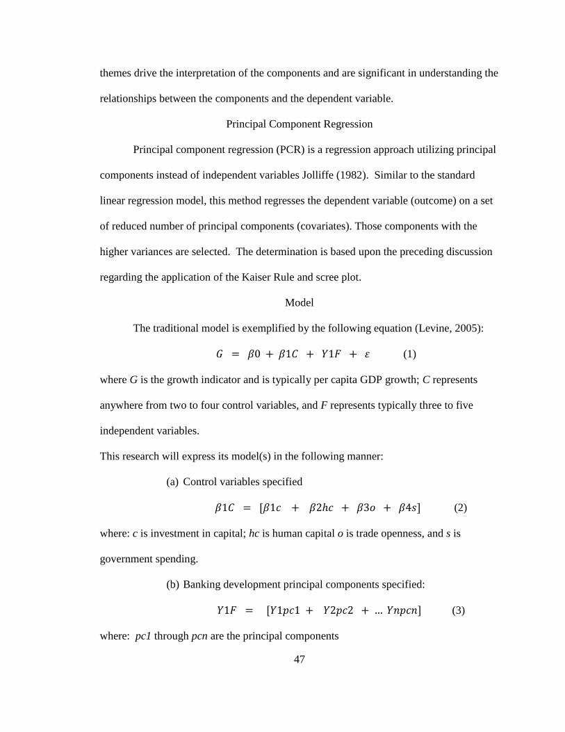
47
themes drive the interpretation of the components and are significant in understanding the
relationships between the components and the dependent variable.
Principal Component Regression
Principal component regression (PCR) is a regression approach utilizing principal
components instead of independent variables Jolliffe (1982). Similar to the standard
linear regression model, this method regresses the dependent variable (outcome) on a set
of reduced number of principal components (covariates). Those components with the
higher variances are selected. The determination is based upon the preceding discussion
regarding the application of the Kaiser Rule and scree plot.
Model
The traditional model is exemplified by the following equation (Levine, 2005):
𝐺 = 𝛽0 + 𝛽1𝐶 + 𝑌1𝐹 + 𝜀 (1)
where G is the growth indicator and is typically per capita GDP growth; C represents
anywhere from two to four control variables, and F represents typically three to five
independent variables.
This research will express its model(s) in the following manner:
(a) Control variables specified
𝛽1𝐶 = [𝛽1𝑐 + 𝛽2ℎ𝑐 + 𝛽3𝑜 + 𝛽4𝑠] (2)
where: c is investment in capital; hc is human capital o is trade openness, and s is
government spending.
(b) Banking development principal components specified:
𝑌1𝐹 = [𝑌1𝑝𝑐1 + 𝑌2𝑝𝑐2 + … 𝑌𝑛𝑝𝑐𝑛] (3)
where: pc1 through pcn are the principal components

48
(c) Aggregate model:
gdp = β0 + β1c + β2hc + β3o + β4s +
Y1pc1 + Y2pc2 + … Ynpcn + ε (4)
where C are the control variables previously mentioned and pc1 through pcn are the
derived components. The number of components (pc1 through pcn) are determined by
the previously mention Kaiser Rule. It is anticipated that number of components may be
five or less.

49
CHAPTER IV – ANALYSIS
Data
This study has not found any body of research that is as inclusive in
characterizing banking development as the twenty-two explanatory variables suggested
herein. Though researchers have increasingly used principal component analysis as a
tool to reveal underlying structures in their data, the number of variables incorporated in
the orthogonal transformation have been typically less than five. Furthermore, they focus
on a broader category of financial sector variables and not the more narrow channel of
banking. The data in his study specifically includes banking variables for the purpose of
regressing economic growth on banking development in Europe, covering less developed,
developing, and developed economies.
The field of data originally included forty-one countries, four control variables
and twenty-two independent variables for a ten year period (2004 – 2013). The forty-one
countries span the European continent and are further subdivided into Western Europe
(19), Central Europe (7), and Eastern Europe (15). Those subdivisions may further
reflect economies that are generally developed, developing, and less developed.
Due to insufficient data, three countries are deleted from the database – Kosovo,
Georgia, and United Kingdom. The reasons for incomplete data vary. Kosovo and
Georgia do not monitor or publish certain banking variables. The United Kingdom
chooses to not make available those banking metrics to the World Bank. The deletion of
these three countries is believed to not have a significant impact upon the methodology.
Twenty-two metrics are chosen to describe banking development. Each of the
independent variables represents one of four dimensions of banking development– access
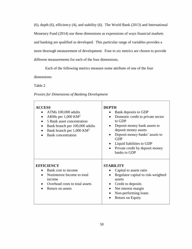
50
(6), depth (6), efficiency (4), and stability (6). The World Bank (2013) and International
Monetary Fund (2014) use these dimensions as expressions of ways financial markets
and banking are qualified as developed. This particular range of variables provides a
more thorough measurement of development. Four to six metrics are chosen to provide
different measurements for each of the four dimensions.
Each of the following metrics measure some attribute of one of the four
dimensions:
Table 2
Proxies for Dimensions of Banking Development
ACCESS
• ATMs 100,000 adults
• ARMs per 1,000 KM2
• 5 Bank asset concentration
• Bank branch per 100,000 adults
• Bank branch per 1,000 KM2
• Bank concentration
DEPTH
• Bank deposits to GDP
• Domestic credit to private sector
to GDP
• Deposit money bank assets to
deposit money assets
• Deposit money banks’ assets to
GDP
• Liquid liabilities to GDP
• Private credit by deposit money
banks to GDP
EFFICIENCY
• Bank cost to income
• Noninterest Income to total
income
• Overhead costs to total assets
• Return on assets
STABILITY
• Capital to assets ratio
• Regulator capital to risk-weighted
assets
• Credit to deposits
• Net interest margin
• Non-performing loans
• Return on Equity

51
Of the metrics listed above, the literature typically restricts its choice to:
a) deposit money bank assets,
b) total bank deposits,
c) liquid liabilities, and
d) private credit by deposit money banks.
These are aggregates of financial institutions balance sheet items and reflect one aspect of
financial development – depth. In contrast, rescaling financial (banking) development
with the World Banks’s four dimensions provides an improved opportunity to measure
and ultimately understanding of development.
The significant addition of independent variables normally raises the risk of
multicollinearity. The collinearity tends to inflate the variance. Furthermore, a large
number of independent variables tend to produce a model that is awkward. Principal
component analysis (PCA) provides a solution. PCA produces components derived from
orthogonally transformed independent variables. Collinearity is resolved and the
resulting number of components should be significantly less than the original number of
variables. Based upon Katchova (2013), the study expects the number of resulting
components for a model to be well less than half of the starting twenty-two independent
variables. Added to that, the strength of the dimensionalities that define development are
determinable from the amount of information about the variance that is retained.
The data is checked for its balance, normality, collinearity, and stationarity.

52
Balance
A balance data set contains all observations in all the time series and panels. As
the Tables 3 and 4 below demonstrate, time series and panel data variables are tested and
determined balanced.
Table 3
Balanced Data Sets
Time Series
tsset cc year, yearly panel variable: cc (strongly balanced)
time variable: year, 2004 to 2013 delta: 1 year
Table 4
Balanced Data Sets
Panel
xtset cc year, yearly panel variable: cc (strongly balanced)
time variable: year, 2004 to 2013 delta: 1 year
Normality
The assumption of normality for the sample distributed is tested. The three tests
applied are Doornick-Hansen, Shapiro-Wilk, and SKtest.
Table 5
Test for Multivariate Normality
Doornik-Hansen chi2 (56) = 28619.6 Prob > chi2 = 0.0000
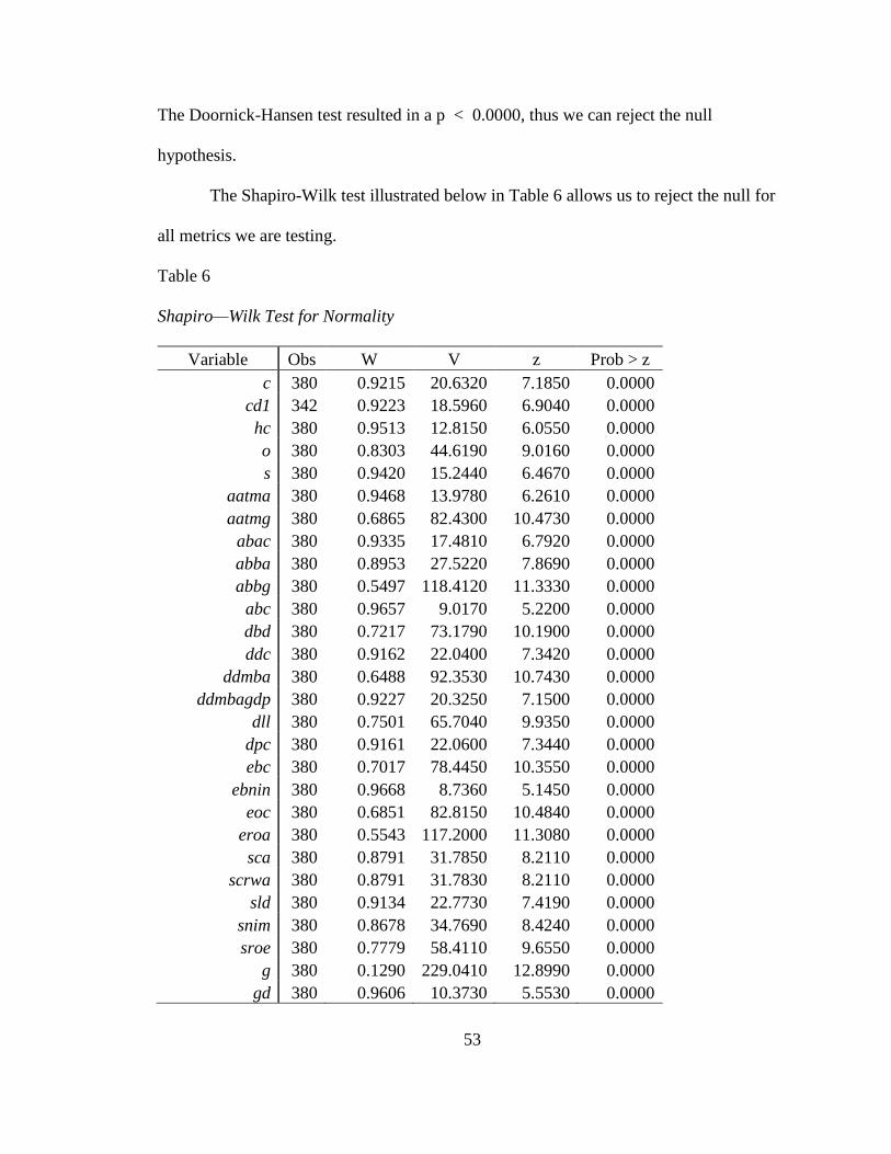
53
The Doornick-Hansen test resulted in a p < 0.0000, thus we can reject the null
hypothesis.
The Shapiro-Wilk test illustrated below in Table 6 allows us to reject the null for
all metrics we are testing.
Table 6
Shapiro—Wilk Test for Normality
Variable Obs W V z Prob > z
c 380 0.9215 20.6320 7.1850 0.0000
cd1 342 0.9223 18.5960 6.9040 0.0000
hc 380 0.9513 12.8150 6.0550 0.0000
o 380 0.8303 44.6190 9.0160 0.0000
s 380 0.9420 15.2440 6.4670 0.0000
aatma 380 0.9468 13.9780 6.2610 0.0000
aatmg 380 0.6865 82.4300 10.4730 0.0000
abac 380 0.9335 17.4810 6.7920 0.0000
abba 380 0.8953 27.5220 7.8690 0.0000
abbg 380 0.5497 118.4120 11.3330 0.0000
abc 380 0.9657 9.0170 5.2200 0.0000
dbd 380 0.7217 73.1790 10.1900 0.0000
ddc 380 0.9162 22.0400 7.3420 0.0000
ddmba 380 0.6488 92.3530 10.7430 0.0000
ddmbagdp 380 0.9227 20.3250 7.1500 0.0000
dll 380 0.7501 65.7040 9.9350 0.0000
dpc 380 0.9161 22.0600 7.3440 0.0000
ebc 380 0.7017 78.4450 10.3550 0.0000
ebnin 380 0.9668 8.7360 5.1450 0.0000
eoc 380 0.6851 82.8150 10.4840 0.0000
eroa 380 0.5543 117.2000 11.3080 0.0000
sca 380 0.8791 31.7850 8.2110 0.0000
scrwa 380 0.8791 31.7830 8.2110 0.0000
sld 380 0.9134 22.7730 7.4190 0.0000
snim 380 0.8678 34.7690 8.4240 0.0000
sroe 380 0.7779 58.4110 9.6550 0.0000
g 380 0.1290 229.0410 12.8990 0.0000
gd 380 0.9606 10.3730 5.5530 0.0000

54
Each of the four control and the twenty-one independent variables have p = 0.0000, thus
we reject the null hypothesis and conclude the data is normally distributed.
The SKtest measures the skewness and kurtosis of the distribution. Table 7
demonstrates the results of the test.
Table 7
Skewness/Kurtosis test for Normality
------- joint ------
Variable Obs Pr(Skewness) Pr(Kurtosis) adj chi2(2) Prob>chi2
c 380 0 0.0001 53.02 0.0000
cd1 342 0 0 47.76 0.0000
hc 380 0 0 56.65 0.0000
o 380 0 0 . 0.0000
s 380 0 0 34.82 0.0000
aatma 380 0 0.0028 37.85 0.0000
aatmg 380 0 0 . 0.0000
abac 380 0 0.0005 29.53 0.0000
abba 380 0 0.0003 60.72 0.0000
abbg 380 0 0 . 0.0000
abc 380 0.2070 0 . 0.0000
dbd 380 0 0 . 0.0000
ddc 380 0 0.0137 43.78 0.0000
ddmba 380 0 0 . 0.0000
ddmbagdp 380 0 0.0058 43.49 0.0000
dll 380 0 0 . 0.0000
dpc 380 0 0.0158 42.99 0.0000
ebc 380 0 0 . 0.0000
ebnin 380 0 0.0012 30.86 0.0000
eoc 380 0 0 . 0.0000
eroa 380 0 0 . 0.0000
sca 380 0 0.0013 58.96 0.0000
scrwa 380 0 0 . 0.0000
sld 380 0 0 66.42 0.0000
snim 380 0 0 . 0.0000
sroe 380 0 0 . 0.0000
g 380 0 0 . 0.0000
gd 380 0 0 40.88 0.0000

55
From the results of the calculations in the far right column, all control and independent
variables have p values less than 0.05, thus allowing a rejection of the null hypothesis
that the data is normally distributed.
For the purposes of this study the normality assumption is unnecessary (Jolliffe,
1982). Following the PCA transformation, principal component regression is run. In
multiple regression models, the estimator is consistent and efficient regardless of
normality of the independent variables. As the sample sizes are not small (n = 380), the t
and f statistics are not adversely affected (Wooldridge, 2010).
Collinearity
As indicated before, this study has an interest in incorporating a larger number of
independent variables that measure banking development in numerous dimensions.
Because of the large number, the regression of growth on these variables is expected to
lead to multicollinearity. Because of this, standard errors will be large and the predictive
power of the model could be inaccurate.
PCA is not negatively affected by collinearity. The test is just the reverse, to be
an effective tool the independent variables need to show collinearity. Table 8
demonstrates that there are significant pairwise correlations of the independent variables.
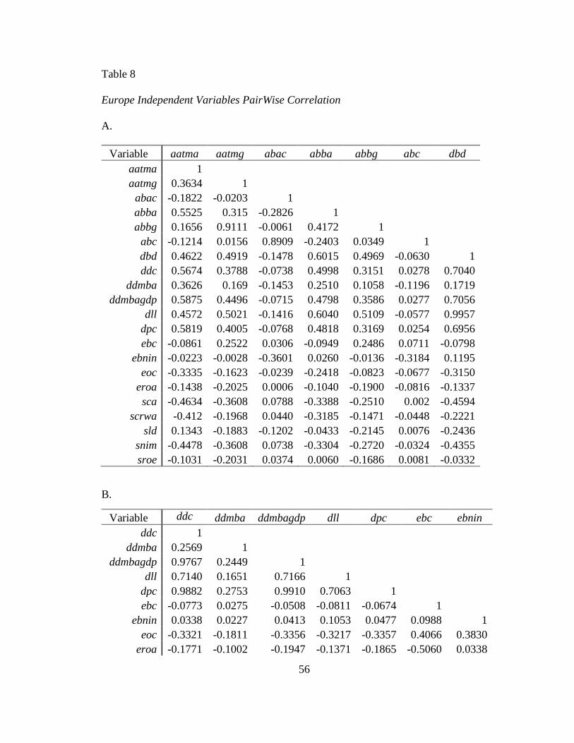
56
Table 8
Europe Independent Variables PairWise Correlation
A.
Variable aatma aatmg abac abba abbg abc dbd
aatma 1
aatmg 0.3634 1
abac -0.1822 -0.0203 1
abba 0.5525 0.315 -0.2826 1
abbg 0.1656 0.9111 -0.0061 0.4172 1
abc -0.1214 0.0156 0.8909 -0.2403 0.0349 1 dbd 0.4622 0.4919 -0.1478 0.6015 0.4969 -0.0630 1
ddc 0.5674 0.3788 -0.0738 0.4998 0.3151 0.0278 0.7040
ddmba 0.3626 0.169 -0.1453 0.2510 0.1058 -0.1196 0.1719
ddmbagdp 0.5875 0.4496 -0.0715 0.4798 0.3586 0.0277 0.7056
dll 0.4572 0.5021 -0.1416 0.6040 0.5109 -0.0577 0.9957
dpc 0.5819 0.4005 -0.0768 0.4818 0.3169 0.0254 0.6956
ebc -0.0861 0.2522 0.0306 -0.0949 0.2486 0.0711 -0.0798
ebnin -0.0223 -0.0028 -0.3601 0.0260 -0.0136 -0.3184 0.1195
eoc -0.3335 -0.1623 -0.0239 -0.2418 -0.0823 -0.0677 -0.3150
eroa -0.1438 -0.2025 0.0006 -0.1040 -0.1900 -0.0816 -0.1337
sca -0.4634 -0.3608 0.0788 -0.3388 -0.2510 0.002 -0.4594
scrwa -0.412 -0.1968 0.0440 -0.3185 -0.1471 -0.0448 -0.2221
sld 0.1343 -0.1883 -0.1202 -0.0433 -0.2145 0.0076 -0.2436
snim -0.4478 -0.3608 0.0738 -0.3304 -0.2720 -0.0324 -0.4355
sroe -0.1031 -0.2031 0.0374 0.0060 -0.1686 0.0081 -0.0332
B.
Variable ddc ddmba ddmbagdp dll dpc ebc ebnin
ddc 1
ddmba 0.2569 1
ddmbagdp 0.9767 0.2449 1
dll 0.7140 0.1651 0.7166 1
dpc 0.9882 0.2753 0.9910 0.7063 1
ebc -0.0773 0.0275 -0.0508 -0.0811 -0.0674 1 ebnin 0.0338 0.0227 0.0413 0.1053 0.0477 0.0988 1
eoc -0.3321 -0.1811 -0.3356 -0.3217 -0.3357 0.4066 0.3830
eroa -0.1771 -0.1002 -0.1947 -0.1371 -0.1865 -0.5060 0.0338
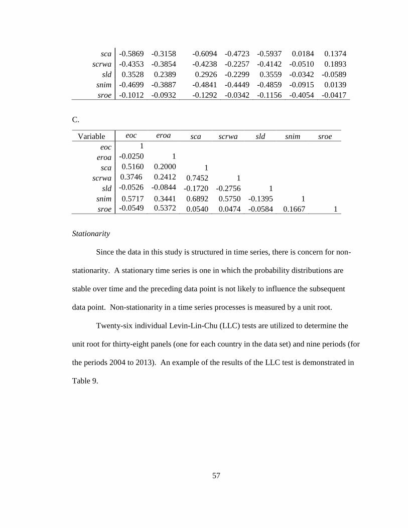
57
sca -0.5869 -0.3158 -0.6094 -0.4723 -0.5937 0.0184 0.1374
scrwa -0.4353 -0.3854 -0.4238 -0.2257 -0.4142 -0.0510 0.1893
sld 0.3528 0.2389 0.2926 -0.2299 0.3559 -0.0342 -0.0589
snim -0.4699 -0.3887 -0.4841 -0.4449 -0.4859 -0.0915 0.0139
sroe -0.1012 -0.0932 -0.1292 -0.0342 -0.1156 -0.4054 -0.0417
C.
Variable eoc eroa sca scrwa sld snim sroe
eoc 1
eroa -0.0250 1
sca 0.5160 0.2000 1
scrwa 0.3746 0.2412 0.7452 1
sld -0.0526 -0.0844 -0.1720 -0.2756 1
snim 0.5717 0.3441 0.6892 0.5750 -0.1395 1 sroe -0.0549 0.5372 0.0540 0.0474 -0.0584 0.1667 1
Stationarity
Since the data in this study is structured in time series, there is concern for non-
stationarity. A stationary time series is one in which the probability distributions are
stable over time and the preceding data point is not likely to influence the subsequent
data point. Non-stationarity in a time series processes is measured by a unit root.
Twenty-six individual Levin-Lin-Chu (LLC) tests are utilized to determine the
unit root for thirty-eight panels (one for each country in the data set) and nine periods (for
the periods 2004 to 2013). An example of the results of the LLC test is demonstrated in
Table 9.
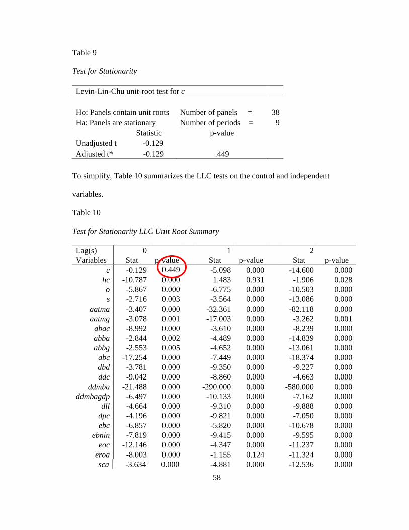
58
Table 9
Test for Stationarity
Levin-Lin-Chu unit-root test for c
Ho: Panels contain unit roots Number of panels = 38
Ha: Panels are stationary Number of periods = 9
Statistic p-value Unadjusted t -0.129
Adjusted t* -0.129 .449
To simplify, Table 10 summarizes the LLC tests on the control and independent
variables.
Table 10
Test for Stationarity LLC Unit Root Summary
Lag(s) 0 1 2
Variables Stat p-value Stat p-value Stat p-value
c -0.129 0.449 -5.098 0.000 -14.600 0.000
hc -10.787 0.000 1.483 0.931 -1.906 0.028
o -5.867 0.000 -6.775 0.000 -10.503 0.000
s -2.716 0.003 -3.564 0.000 -13.086 0.000
aatma -3.407 0.000 -32.361 0.000 -82.118 0.000
aatmg -3.078 0.001 -17.003 0.000 -3.262 0.001
abac -8.992 0.000 -3.610 0.000 -8.239 0.000
abba -2.844 0.002 -4.489 0.000 -14.839 0.000
abbg -2.553 0.005 -4.652 0.000 -13.061 0.000
abc -17.254 0.000 -7.449 0.000 -18.374 0.000
dbd -3.781 0.000 -9.350 0.000 -9.227 0.000
ddc -9.042 0.000 -8.860 0.000 -4.663 0.000
ddmba -21.488 0.000 -290.000 0.000 -580.000 0.000
ddmbagdp -6.497 0.000 -10.133 0.000 -7.162 0.000
dll -4.664 0.000 -9.310 0.000 -9.888 0.000
dpc -4.196 0.000 -9.821 0.000 -7.050 0.000
ebc -6.857 0.000 -5.820 0.000 -10.678 0.000
ebnin -7.819 0.000 -9.415 0.000 -9.595 0.000
eoc -12.146 0.000 -4.347 0.000 -11.237 0.000
eroa -8.003 0.000 -1.155 0.124 -11.324 0.000
sca -3.634 0.000 -4.881 0.000 -12.536 0.000
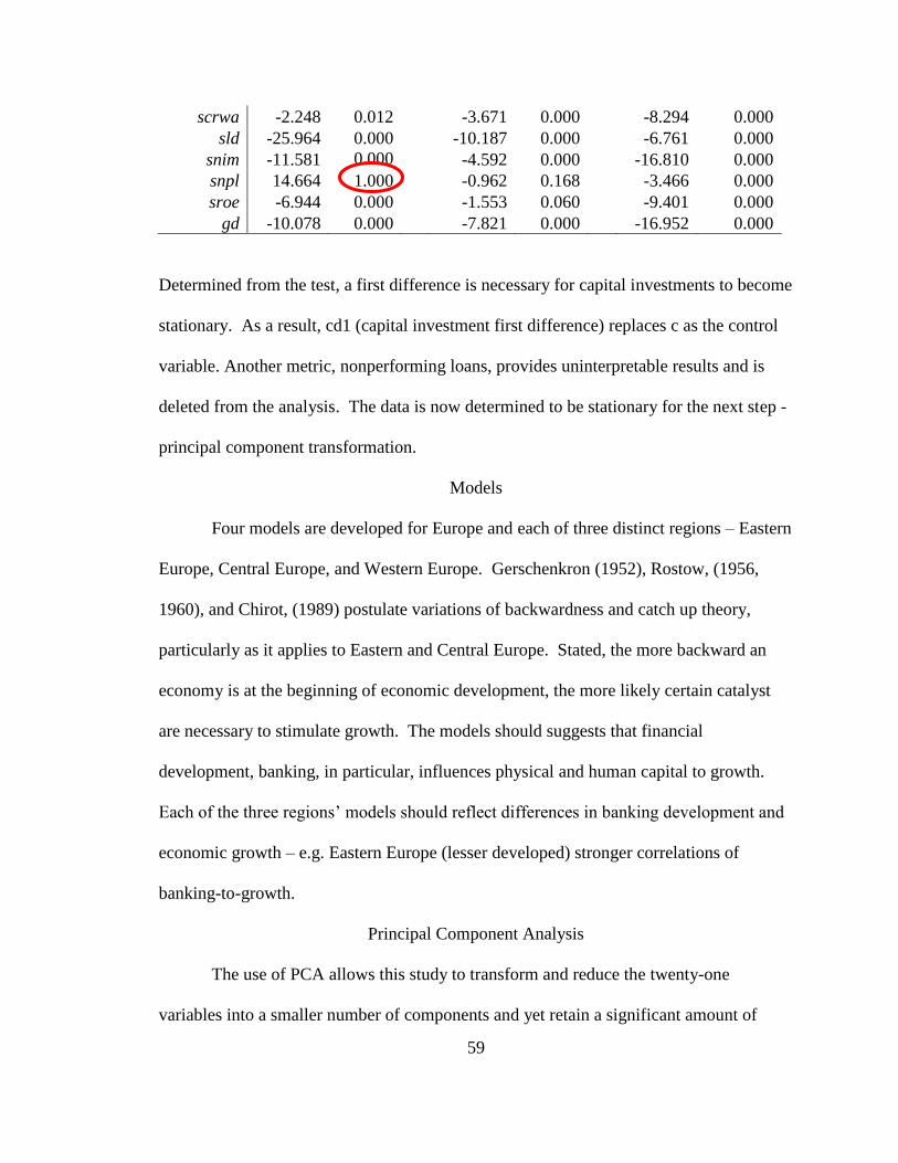
59
scrwa -2.248 0.012 -3.671 0.000 -8.294 0.000
sld -25.964 0.000 -10.187 0.000 -6.761 0.000
snim -11.581 0.000 -4.592 0.000 -16.810 0.000
snpl 14.664 1.000 -0.962 0.168 -3.466 0.000
sroe -6.944 0.000 -1.553 0.060 -9.401 0.000
gd -10.078 0.000 -7.821 0.000 -16.952 0.000
Determined from the test, a first difference is necessary for capital investments to become
stationary. As a result, cd1 (capital investment first difference) replaces c as the control
variable. Another metric, nonperforming loans, provides uninterpretable results and is
deleted from the analysis. The data is now determined to be stationary for the next step -
principal component transformation.
Models
Four models are developed for Europe and each of three distinct regions – Eastern
Europe, Central Europe, and Western Europe. Gerschenkron (1952), Rostow, (1956,
1960), and Chirot, (1989) postulate variations of backwardness and catch up theory,
particularly as it applies to Eastern and Central Europe. Stated, the more backward an
economy is at the beginning of economic development, the more likely certain catalyst
are necessary to stimulate growth. The models should suggests that financial
development, banking, in particular, influences physical and human capital to growth.
Each of the three regions’ models should reflect differences in banking development and
economic growth – e.g. Eastern Europe (lesser developed) stronger correlations of
banking-to-growth.
Principal Component Analysis
The use of PCA allows this study to transform and reduce the twenty-one
variables into a smaller number of components and yet retain a significant amount of

60
information about the variances. The components themselves are correlated with the
variables. Interpreting the components references back to those variables most strongly
correlated. From those variables, we may label the component in a manner that describes
its effect on the dependent variable.
The following are the steps in PCA:
a. Determine sampling adequacy
b. Transform variables into components;
c. Apply the Kaiser rule and scree plot to determine the number of components
to retain;
d. Rotate the orthogonal relationships using Varimax and Promax
e. Review the greatest magnitudes of the eigenvector loadings (correlation
coefficients);
f. Determine a descriptive label for each component based upon the
concentration of variables with the greatest loadings;
g. Perform an initial principal component regression to test statistical
significance
h. Specify the model with significant variables and components
Sampling Adequacy
As mentioned before, PCA necessarily requires the data to have a degree of
collinearity to be suitable for transformation. The Kaiser-Meyer-Olkin (KMO) test
measures the data’s suitability by providing the proportion of variance which might be
caused by underlying factors. KMO values range from 0 to 1. High values indicate
usefulness. Both William et al. (2010) and Parinet et al. (2004) state the data is adequate
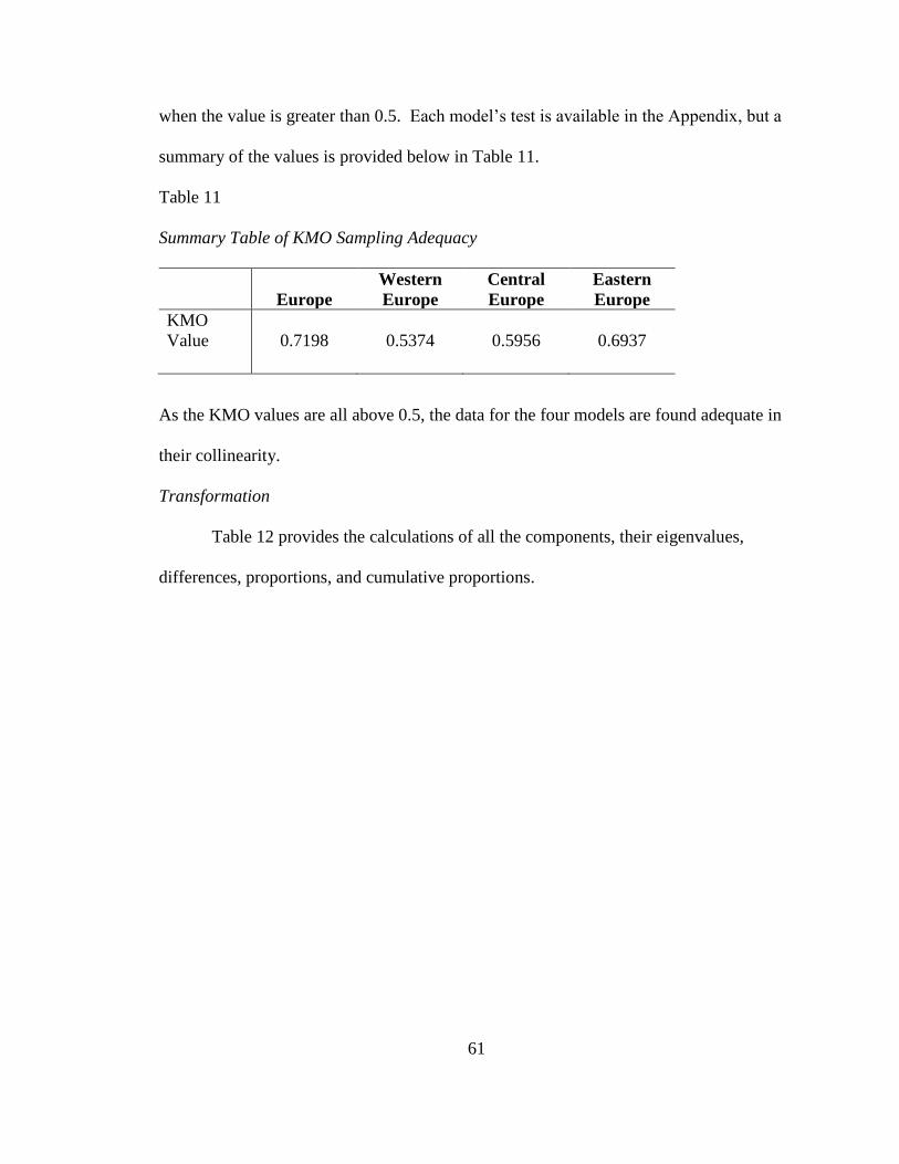
61
when the value is greater than 0.5. Each model’s test is available in the Appendix, but a
summary of the values is provided below in Table 11.
Table 11
Summary Table of KMO Sampling Adequacy
Europe
Western
Europe
Central
Europe
Eastern
Europe
KMO
Value 0.7198
0.5374
0.5956
0.6937
As the KMO values are all above 0.5, the data for the four models are found adequate in
their collinearity.
Transformation
Table 12 provides the calculations of all the components, their eigenvalues,
differences, proportions, and cumulative proportions.
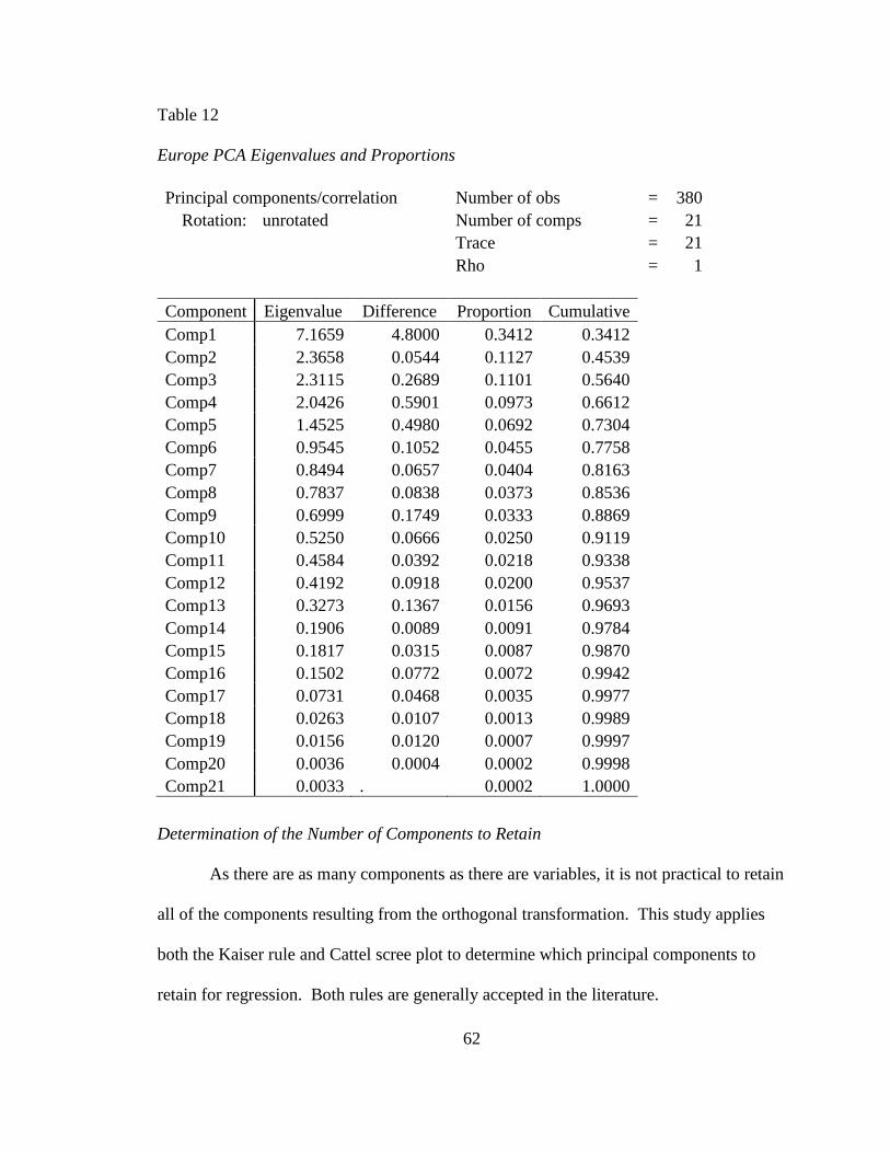
62
Table 12
Europe PCA Eigenvalues and Proportions
Principal components/correlation Number of obs = 380
Rotation: unrotated Number of comps = 21
Trace = 21
Rho = 1
Component Eigenvalue Difference Proportion Cumulative
Comp1 7.1659 4.8000 0.3412 0.3412
Comp2 2.3658 0.0544 0.1127 0.4539
Comp3 2.3115 0.2689 0.1101 0.5640
Comp4 2.0426 0.5901 0.0973 0.6612
Comp5 1.4525 0.4980 0.0692 0.7304
Comp6 0.9545 0.1052 0.0455 0.7758
Comp7 0.8494 0.0657 0.0404 0.8163
Comp8 0.7837 0.0838 0.0373 0.8536
Comp9 0.6999 0.1749 0.0333 0.8869
Comp10 0.5250 0.0666 0.0250 0.9119
Comp11 0.4584 0.0392 0.0218 0.9338
Comp12 0.4192 0.0918 0.0200 0.9537
Comp13 0.3273 0.1367 0.0156 0.9693
Comp14 0.1906 0.0089 0.0091 0.9784
Comp15 0.1817 0.0315 0.0087 0.9870
Comp16 0.1502 0.0772 0.0072 0.9942
Comp17 0.0731 0.0468 0.0035 0.9977
Comp18 0.0263 0.0107 0.0013 0.9989
Comp19 0.0156 0.0120 0.0007 0.9997
Comp20 0.0036 0.0004 0.0002 0.9998
Comp21 0.0033 . 0.0002 1.0000
Determination of the Number of Components to Retain
As there are as many components as there are variables, it is not practical to retain
all of the components resulting from the orthogonal transformation. This study applies
both the Kaiser rule and Cattel scree plot to determine which principal components to
retain for regression. Both rules are generally accepted in the literature.
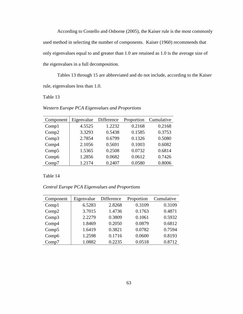
63
According to Costello and Osborne (2005), the Kaiser rule is the most commonly
used method in selecting the number of components. Kaiser (1960) recommends that
only eigenvalues equal to and greater than 1.0 are retained as 1.0 is the average size of
the eigenvalues in a full decomposition.
Tables 13 through 15 are abbreviated and do not include, according to the Kaiser
rule, eigenvalues less than 1.0.
Table 13
Western Europe PCA Eigenvalues and Proportions
Component Eigenvalue Difference Proportion Cumulative
Comp1 4.5525 1.2232 0.2168 0.2168
Comp2 3.3293 0.5438 0.1585 0.3753
Comp3 2.7854 0.6799 0.1326 0.5080
Comp4 2.1056 0.5691 0.1003 0.6082
Comp5 1.5365 0.2508 0.0732 0.6814
Comp6 1.2856 0.0682 0.0612 0.7426
Comp7 1.2174 0.2407 0.0580 0.8006
Table 14
Central Europe PCA Eigenvalues and Proportions
Component Eigenvalue Difference Proportion Cumulative
Comp1 6.5283 2.8268 0.3109 0.3109
Comp2 3.7015 1.4736 0.1763 0.4871
Comp3 2.2279 0.3809 0.1061 0.5932
Comp4 1.8469 0.2050 0.0879 0.6812
Comp5 1.6419 0.3821 0.0782 0.7594
Comp6 1.2598 0.1716 0.0600 0.8193
Comp7 1.0882 0.2235 0.0518 0.8712
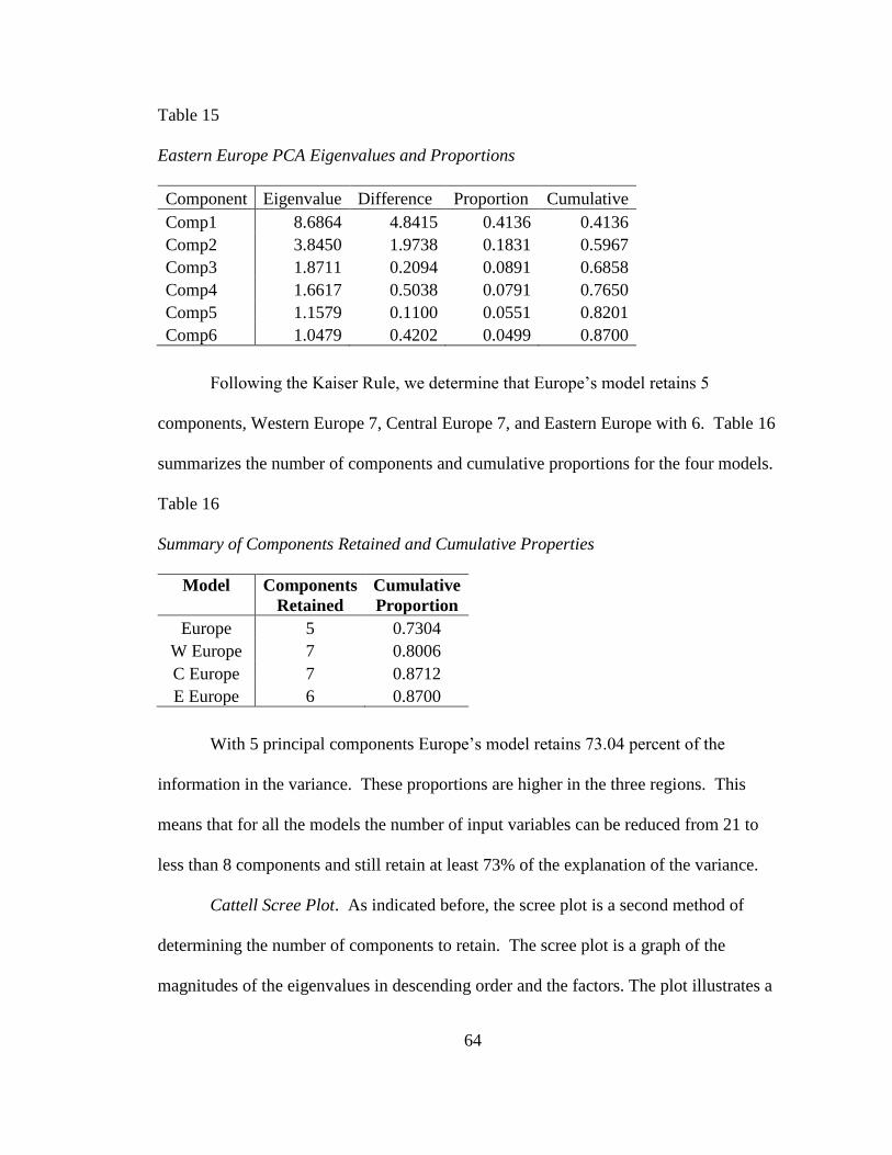
64
Table 15
Eastern Europe PCA Eigenvalues and Proportions
Component Eigenvalue Difference Proportion Cumulative
Comp1 8.6864 4.8415 0.4136 0.4136
Comp2 3.8450 1.9738 0.1831 0.5967
Comp3 1.8711 0.2094 0.0891 0.6858
Comp4 1.6617 0.5038 0.0791 0.7650
Comp5 1.1579 0.1100 0.0551 0.8201
Comp6 1.0479 0.4202 0.0499 0.8700
Following the Kaiser Rule, we determine that Europe’s model retains 5
components, Western Europe 7, Central Europe 7, and Eastern Europe with 6. Table 16
summarizes the number of components and cumulative proportions for the four models.
Table 16
Summary of Components Retained and Cumulative Properties
Model
Components
Retained
Cumulative
Proportion
Europe 5 0.7304
W Europe 7 0.8006
C Europe 7 0.8712
E Europe 6 0.8700
With 5 principal components Europe’s model retains 73.04 percent of the
information in the variance. These proportions are higher in the three regions. This
means that for all the models the number of input variables can be reduced from 21 to
less than 8 components and still retain at least 73% of the explanation of the variance.
Cattell Scree Plot. As indicated before, the scree plot is a second method of
determining the number of components to retain. The scree plot is a graph of the
magnitudes of the eigenvalues in descending order and the factors. The plot illustrates a
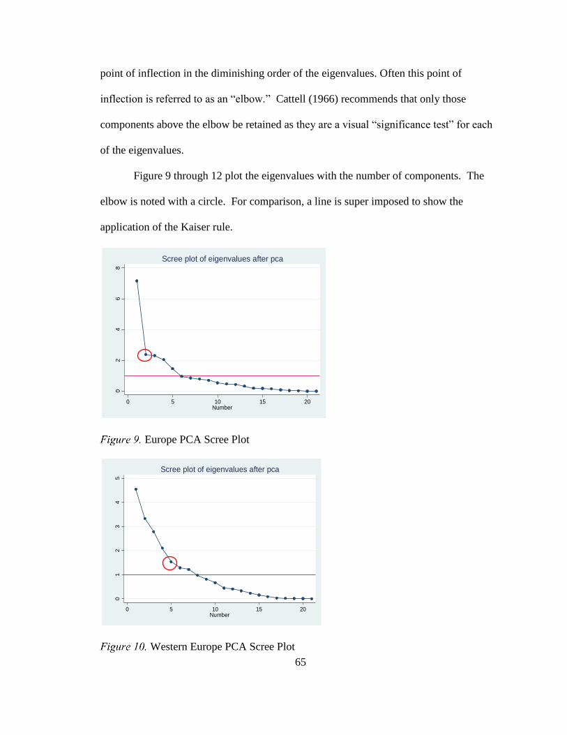
65
point of inflection in the diminishing order of the eigenvalues. Often this point of
inflection is referred to as an “elbow.” Cattell (1966) recommends that only those
components above the elbow be retained as they are a visual “significance test” for each
of the eigenvalues.
Figure 9 through 12 plot the eigenvalues with the number of components. The
elbow is noted with a circle. For comparison, a line is super imposed to show the
application of the Kaiser rule.
Europe PCA Scree Plot
Western Europe PCA Scree Plot
02
46
8
Eig
enva
lues
0 5 10 15 20Number
Scree plot of eigenvalues after pca
01
23
45
Eig
enva
lues
0 5 10 15 20Number
Scree plot of eigenvalues after pca
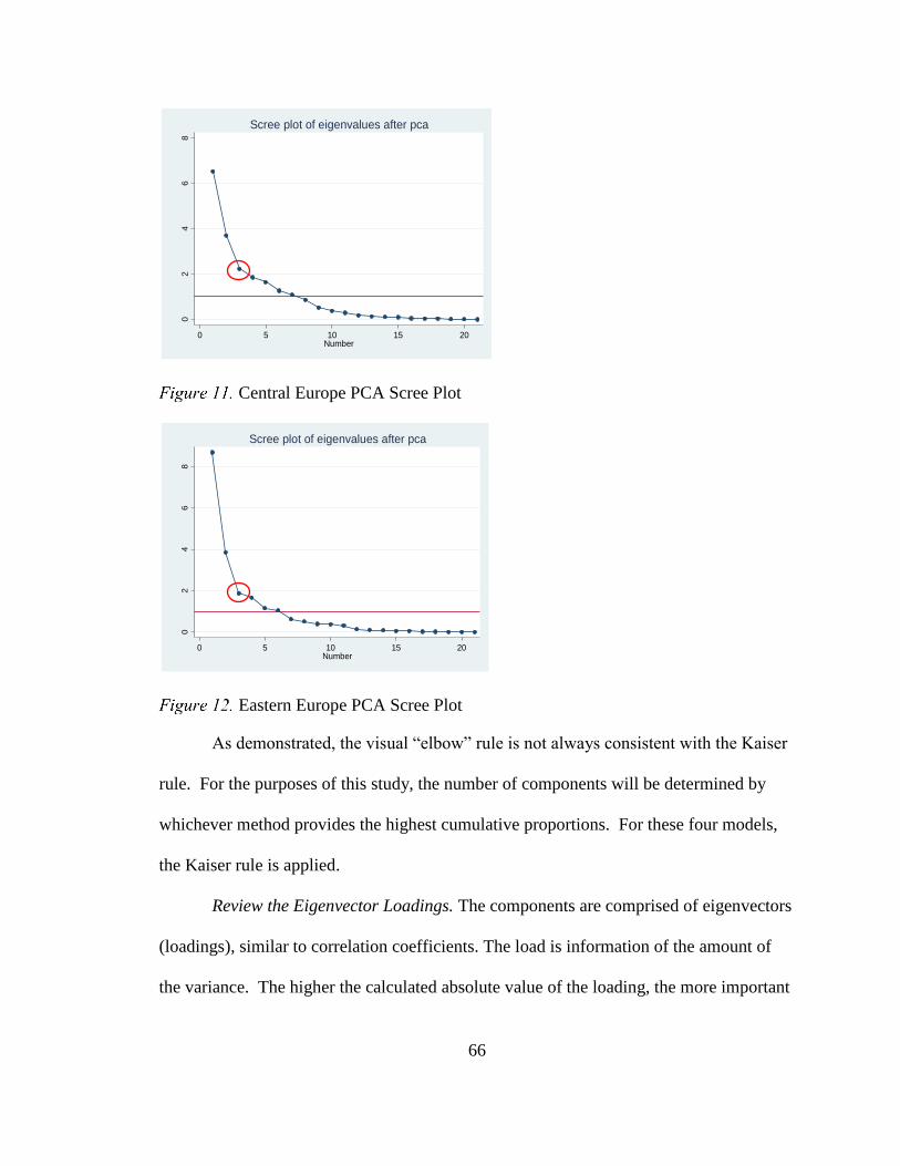
66
Central Europe PCA Scree Plot
Eastern Europe PCA Scree Plot
As demonstrated, the visual “elbow” rule is not always consistent with the Kaiser
rule. For the purposes of this study, the number of components will be determined by
whichever method provides the highest cumulative proportions. For these four models,
the Kaiser rule is applied.
Review the Eigenvector Loadings. The components are comprised of eigenvectors
(loadings), similar to correlation coefficients. The load is information of the amount of
the variance. The higher the calculated absolute value of the loading, the more important
02
46
8
Eig
enva
lues
0 5 10 15 20Number
Scree plot of eigenvalues after pca
02
46
8
Eig
enva
lues
0 5 10 15 20Number
Scree plot of eigenvalues after pca
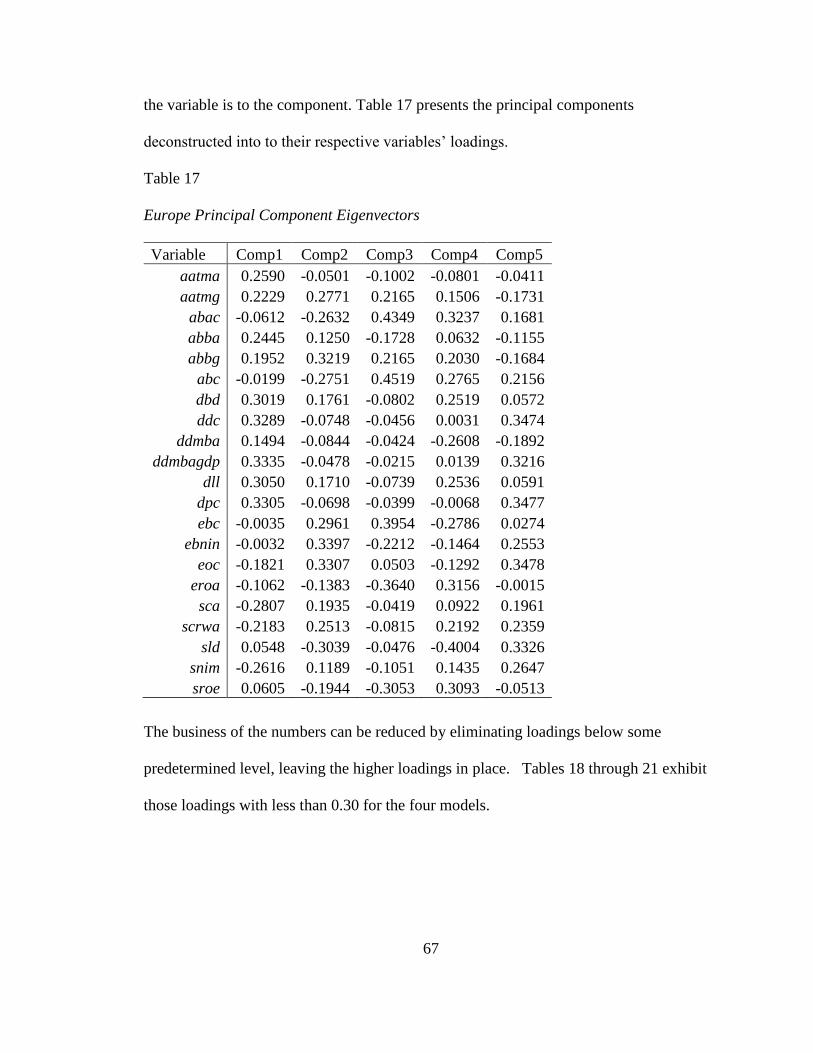
67
the variable is to the component. Table 17 presents the principal components
deconstructed into to their respective variables’ loadings.
Table 17
Europe Principal Component Eigenvectors
Variable Comp1 Comp2 Comp3 Comp4 Comp5
aatma 0.2590 -0.0501 -0.1002 -0.0801 -0.0411
aatmg 0.2229 0.2771 0.2165 0.1506 -0.1731
abac -0.0612 -0.2632 0.4349 0.3237 0.1681
abba 0.2445 0.1250 -0.1728 0.0632 -0.1155
abbg 0.1952 0.3219 0.2165 0.2030 -0.1684
abc -0.0199 -0.2751 0.4519 0.2765 0.2156
dbd 0.3019 0.1761 -0.0802 0.2519 0.0572
ddc 0.3289 -0.0748 -0.0456 0.0031 0.3474
ddmba 0.1494 -0.0844 -0.0424 -0.2608 -0.1892
ddmbagdp 0.3335 -0.0478 -0.0215 0.0139 0.3216
dll 0.3050 0.1710 -0.0739 0.2536 0.0591
dpc 0.3305 -0.0698 -0.0399 -0.0068 0.3477
ebc -0.0035 0.2961 0.3954 -0.2786 0.0274
ebnin -0.0032 0.3397 -0.2212 -0.1464 0.2553
eoc -0.1821 0.3307 0.0503 -0.1292 0.3478
eroa -0.1062 -0.1383 -0.3640 0.3156 -0.0015
sca -0.2807 0.1935 -0.0419 0.0922 0.1961
scrwa -0.2183 0.2513 -0.0815 0.2192 0.2359
sld 0.0548 -0.3039 -0.0476 -0.4004 0.3326
snim -0.2616 0.1189 -0.1051 0.1435 0.2647
sroe 0.0605 -0.1944 -0.3053 0.3093 -0.0513
The business of the numbers can be reduced by eliminating loadings below some
predetermined level, leaving the higher loadings in place. Tables 18 through 21 exhibit
those loadings with less than 0.30 for the four models.
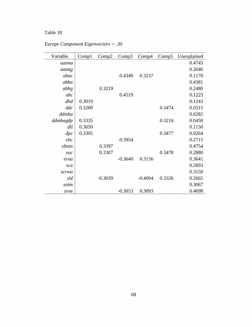
68
Table 18
Europe Component Eigenvectors > .30
Variable Comp1 Comp2 Comp3 Comp4 Comp5 Unexplained
aatma 0.4745
aatmg 0.2640
abac 0.4349 0.3237 0.1170
abba 0.4381
abbg 0.3219 0.2480
abc 0.4519 0.1225
dbd 0.3019 0.1243
ddc 0.3289 0.3474 0.0315
ddmba 0.6282
ddmbagdp 0.3335 0.3216 0.0458
dll 0.3050 0.1150
dpc 0.3305 0.3477 0.0264
ebc 0.3954 0.2715
ebnin 0.3397 0.4754
eoc 0.3307 0.3478 0.2880
eroa -0.3640 0.3156 0.3641
sca 0.2693
scrwa 0.3150
sld -0.3039 -0.4004 0.3326 0.2665
snim 0.3067
sroe -0.3053 0.3093 0.4698
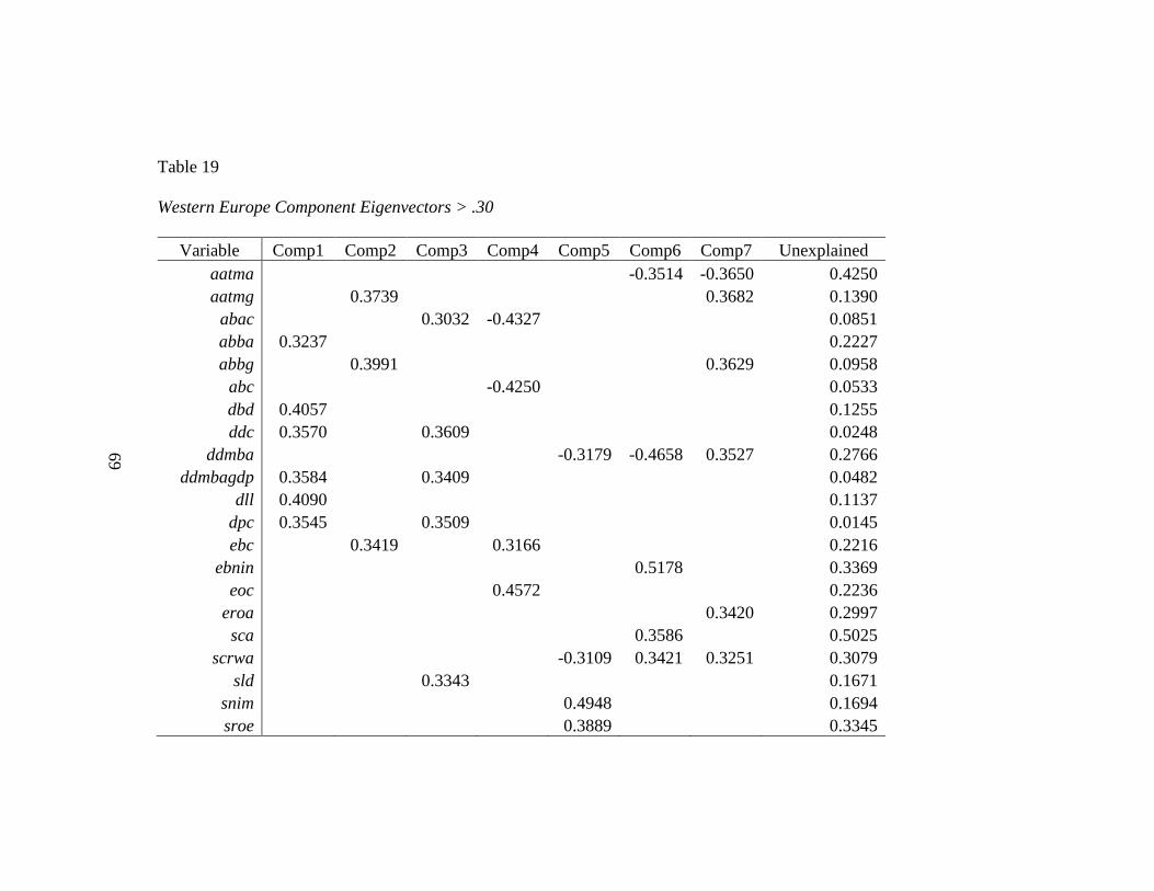
69
Table 19
Western Europe Component Eigenvectors > .30
Variable Comp1 Comp2 Comp3 Comp4 Comp5 Comp6 Comp7 Unexplained
aatma -0.3514 -0.3650 0.4250
aatmg 0.3739 0.3682 0.1390
abac 0.3032 -0.4327 0.0851
abba 0.3237 0.2227
abbg 0.3991 0.3629 0.0958
abc -0.4250 0.0533
dbd 0.4057 0.1255
ddc 0.3570 0.3609 0.0248
ddmba -0.3179 -0.4658 0.3527 0.2766
ddmbagdp 0.3584 0.3409 0.0482
dll 0.4090 0.1137
dpc 0.3545 0.3509 0.0145
ebc 0.3419 0.3166 0.2216
ebnin 0.5178 0.3369
eoc 0.4572 0.2236
eroa 0.3420 0.2997
sca 0.3586 0.5025
scrwa -0.3109 0.3421 0.3251 0.3079
sld 0.3343 0.1671
snim 0.4948 0.1694
sroe 0.3889 0.3345
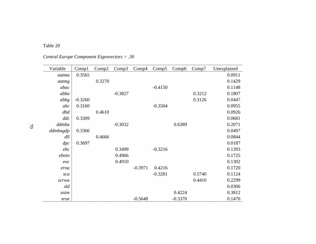
70
Table 20
Central Europe Component Eigenvectors > .30
Variable Comp1 Comp2 Comp3 Comp4 Comp5 Comp6 Comp7 Unexplained
aatma 0.3565 0.0911
aatmg 0.3270 0.1429
abac -0.4150 0.1148
abba -0.3827 0.3212 0.1807
abbg -0.3260 0.3126 0.0447
abc 0.3160 -0.3504 0.0955
dbd 0.4610 0.0926
ddc 0.3309 0.0681
ddmba -0.3032 0.6389 0.2071
ddmbagdp 0.3366 0.0497
dll 0.4666 0.0844
dpc 0.3697 0.0187
ebc 0.3499 -0.3216 0.1393
ebnin 0.4966 0.1725
eoc 0.4910 0.1302
eroa -0.3971 0.4216 0.1720
sca -0.3281 0.5740 0.1124
scrwa 0.4410 0.2299
sld 0.0306
snim 0.4224 0.3812
sroe -0.5648 -0.3370 0.1470
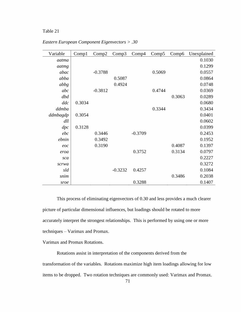
71
Table 21
Eastern European Component Eigenvectors > .30
Variable Comp1 Comp2 Comp3 Comp4 Comp5 Comp6 Unexplained
aatma 0.1030
aatmg 0.1299
abac -0.3788 0.5069 0.0557
abba 0.5087 0.0864
abbg 0.4924 0.0748
abc -0.3812 0.4744 0.0369
dbd 0.3063 0.0289
ddc 0.3034 0.0680
ddmba 0.3344 0.3434
ddmbagdp 0.3054 0.0401
dll 0.0602
dpc 0.3128 0.0399
ebc 0.3446 -0.3709 0.2453
ebnin 0.3492 0.1952
eoc 0.3190 0.4087 0.1397
eroa 0.3752 0.3134 0.0797
sca 0.2227
scrwa 0.3272
sld -0.3232 0.4257 0.1084
snim 0.3486 0.2038
sroe 0.3288 0.1407
This process of eliminating eigenvectors of 0.30 and less provides a much clearer
picture of particular dimensional influences, but loadings should be rotated to more
accurately interpret the strongest relationships. This is performed by using one or more
techniques – Varimax and Promax.
Varimax and Promax Rotations.
Rotations assist in interpretation of the components derived from the
transformation of the variables. Rotations maximize high item loadings allowing for low
items to be dropped. Two rotation techniques are commonly used: Varimax and Promax.

72
The Varimax rotation are orthogonal, preserving the perpendicularity of the axis,
and produces components that are uncorrelated and independent (Kaiser, 1958.) It takes
its name from the maximization of the sum of the variances of the squared correlations
between variables and factors. In contrast, Promax rotations are oblique, interrelated and
results in component structures that are correlated. The objective in using the two
rotations is to provide easier and simpler interpretations. According to Finch (2006) the
two approaches are equally able to identify the underlying structures.
The following tables, 22 through 25, show the Varimax rotations. Groupings of
dimensions are circled. These groupings will aid in the interpretation and labeling of the
components for the PC regression.
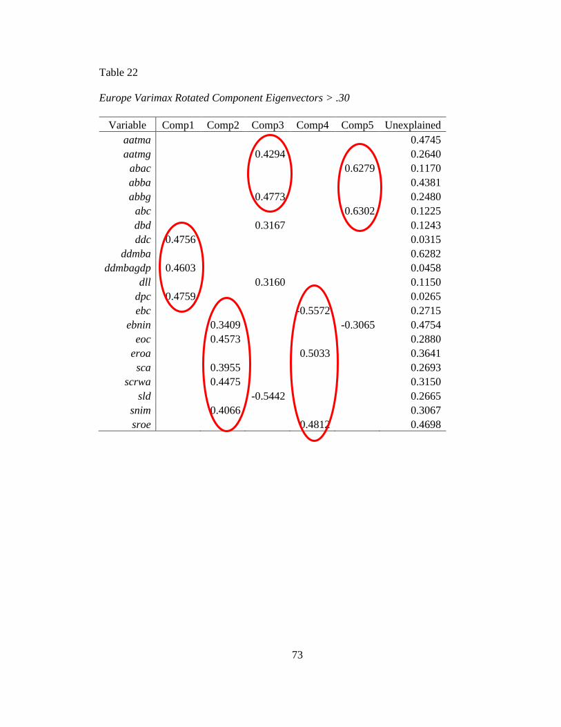
73
Table 22
Europe Varimax Rotated Component Eigenvectors > .30
Variable Comp1 Comp2 Comp3 Comp4 Comp5 Unexplained
aatma
0.4745
aatmg 0.4294 0.2640
abac 0.6279 0.1170
abba 0.4381
abbg 0.4773 0.2480
abc 0.6302 0.1225
dbd 0.3167 0.1243
ddc 0.4756 0.0315
ddmba 0.6282
ddmbagdp 0.4603 0.0458
dll 0.3160
0.1150
dpc 0.4759
0.0265
ebc -0.5572 0.2715
ebnin 0.3409 -0.3065 0.4754
eoc 0.4573 0.2880
eroa 0.5033 0.3641
sca 0.3955 0.2693
scrwa 0.4475 0.3150
sld -0.5442 0.2665
snim 0.4066 0.3067
sroe 0.4812 0.4698
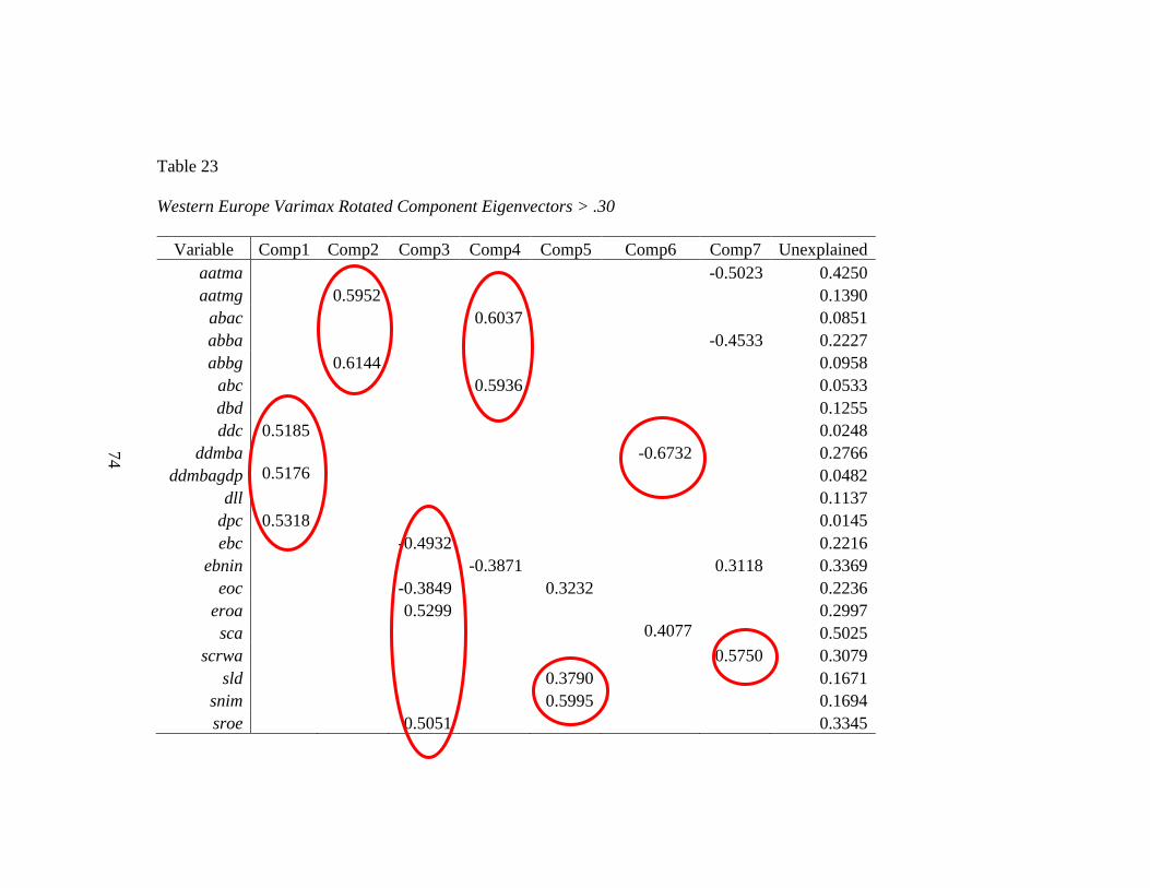
74
Table 23
Western Europe Varimax Rotated Component Eigenvectors > .30
Variable Comp1 Comp2 Comp3 Comp4 Comp5 Comp6 Comp7 Unexplained
aatma -0.5023 0.4250
aatmg 0.5952 0.1390
abac 0.6037 0.0851
abba
-0.4533 0.2227
abbg 0.6144 0.0958
abc 0.5936 0.0533
dbd
0.1255
ddc 0.5185 0.0248
ddmba -0.6732 0.2766
ddmbagdp 0.5176 0.0482
dll 0.1137
dpc 0.5318
0.0145
ebc -0.4932 0.2216
ebnin -0.3871 0.3118 0.3369
eoc -0.3849 0.3232 0.2236
eroa 0.5299 0.2997
sca 0.4077 0.5025
scrwa
0.5750 0.3079
sld 0.3790 0.1671
snim 0.5995 0.1694
sroe 0.5051 0.3345
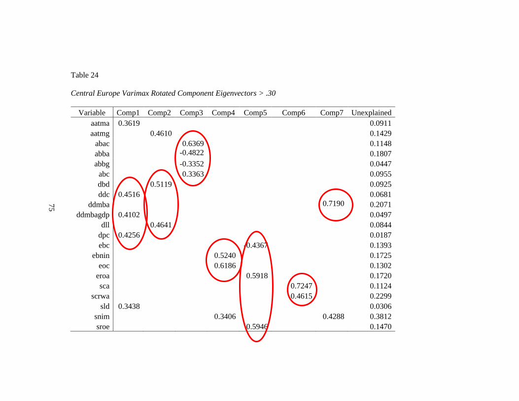
75
Table 24
Central Europe Varimax Rotated Component Eigenvectors > .30
Variable Comp1 Comp2 Comp3 Comp4 Comp5 Comp6 Comp7 Unexplained
aatma 0.3619 0.0911
aatmg 0.4610 0.1429
abac 0.6369 0.1148
abba -0.4822 0.1807
abbg -0.3352 0.0447
abc 0.3363 0.0955
dbd 0.5119 0.0925
ddc 0.4516 0.0681
ddmba
0.7190 0.2071
ddmbagdp 0.4102 0.0497
dll 0.4641 0.0844
dpc 0.4256 0.0187
ebc -0.4367 0.1393
ebnin 0.5240
0.1725
eoc 0.6186 0.1302
eroa 0.5918
0.1720
sca 0.7247 0.1124
scrwa 0.4615 0.2299
sld 0.3438 0.0306
snim 0.3406 0.4288 0.3812
sroe 0.5946 0.1470
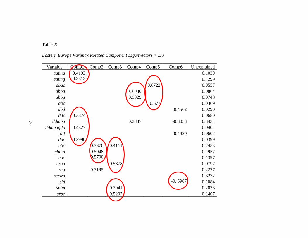
76
Table 25
Eastern Europe Varimax Rotated Component Eigenvectors > .30
Variable Comp1 Comp2 Comp3 Comp4 Comp5 Comp6 Unexplained
aatma 0.4193
0.1030
aatmg 0.3813 0.1299
abac 0.6722 0.0557
abba 0. 6030 0.0864
abbg 0.5929
0.0748
abc 0.677 0.0369
dbd 0.4562 0.0290
ddc 0.3874 0.0680
ddmba
0.3837 -0.3053 0.3434
ddmbagdp 0.4327 0.0401
dll 0.4820 0.0602
dpc 0.3990 0.0399
ebc 0.3370 -0.4111 0.2453
ebnin 0.5048 0.1952
eoc 0.5700
0.1397
eroa 0.5878 0.0797
sca 0.3195 0.2227
scrwa 0.3272
sld -0. 5967 0.1084
snim 0.3941 0.2038
sroe 0.5207 0.1407

77
Determine a Descriptive Label for each Component Based Upon the Concentration of
Variables with the Greatest Loadings
As components are the transformation of the independent variables, they can
share multiple aspects of various dimensions. That is to say, components express more
than just one dimension or the other. Combinations may express internal (operational)
aspects – how efficient banking is managed and the strength and solvency of the
institutions. Combinations may also express external (diffusion) dynamics – how
accessible is banking to the customer base and the depth of the kinds and number of
banking services. When components are blended dimensions they create yet other
descriptors of banking development. When a component shares efficiency and stability
dimensions, this is an internal operations aspect, and when access and depth are
predominant, there is an external aspect of diffusion. These will be used also in the
following models.
Interpretation. Variables are Transformed into Components. Examining the
combination of the highest loading variables lends insight into the interpretation of the
structure of the component. The goal is to find a cluster of variables that define a
component (Katchova, 2013.) As the components’ structure is interpreted, a meaningful
description or theme may be exposed. The components are typically labeled after the
themes they express. This descriptive label is helpful in understanding the model
following principal component regression.

78
Europe Summary of Results:
Comp 1-specifically centered on depth metrics, labeled depth credit;
Comp 2-mainly combined both efficiency and stability, labeled operations costs;
Comp 3-heavily concentrated with access but also includes stability,
labeled access branching;
Comp 4-mostly combines efficiency and stability, labeled operations cost; and,
Comp 5-heavily concentrated with access metrics, access credit.
Overall, the highest loadings came from access credit and access concentration
Western Europe Summary of Results:
Comp 1-specifically centered on depth metrics, labeled depth credit;
Comp 2-specifically centered on access metrics, labeled access branches;
Comp 3-heavily concentrated with efficiency but also includes strong stability,
labeled operations;
Comp 4-heavily loaded with access metrics, labeled access concentration;
Comp 5-heavily concentrated with stability metrics, labeled depth assets;
Comp 6-heavily concentrated with depth metrics, labeled depth assets; and,
Comp 7-strong concentration of both access and stability metrics, labeled access
atms.
Overall, the highest loadings came from access and depth.
Central Europe Summary of Results:
Comp 1-mostly centered on depth metrics, labeled depth credit;
Comp 2-mostly centered on depth metrics, labeled depth deposits;
Comp 3-specifically concentrated with access metrics, labeled access

79
concentration;
Comp 4-heavily loaded with efficiency metrics, labeled efficiency costs;
Comp 5-shares efficiency and stability metrics, labeled operations return;
Comp 6-specifically concentrated with stability metrics, labeled stable capital;
and,
Comp 7-strong concentration of depth metrics, labeled depth assets
Overall, the highest loadings came from stable capital and depth assets
Eastern Europe Summary of Results:
Comp 1-shares access and depth metrics, labeled diffusion assets;
Comp 2- mostly centered on efficiency metrics, labeled efficiency margin;
Comp 3-shares efficiency and stability metrics, labeled operations return;
Comp 4-heavily loaded with access metrics, labeled access branches;
Comp 5-specifically loaded with access metrics, labeled access credit; and
Comp 6-shares depth and stability metrics, labeled stability leverage.
Overall, the highest loadings came from solvency capital and depth assets
Below is an example of an initial principal component regression performed to
test statistical significance. Tables 26 and 27 illustrate the initial and secondary
proposals. Variables in Table 26 that fail to be significant (circled) are deleted in the
second regression.
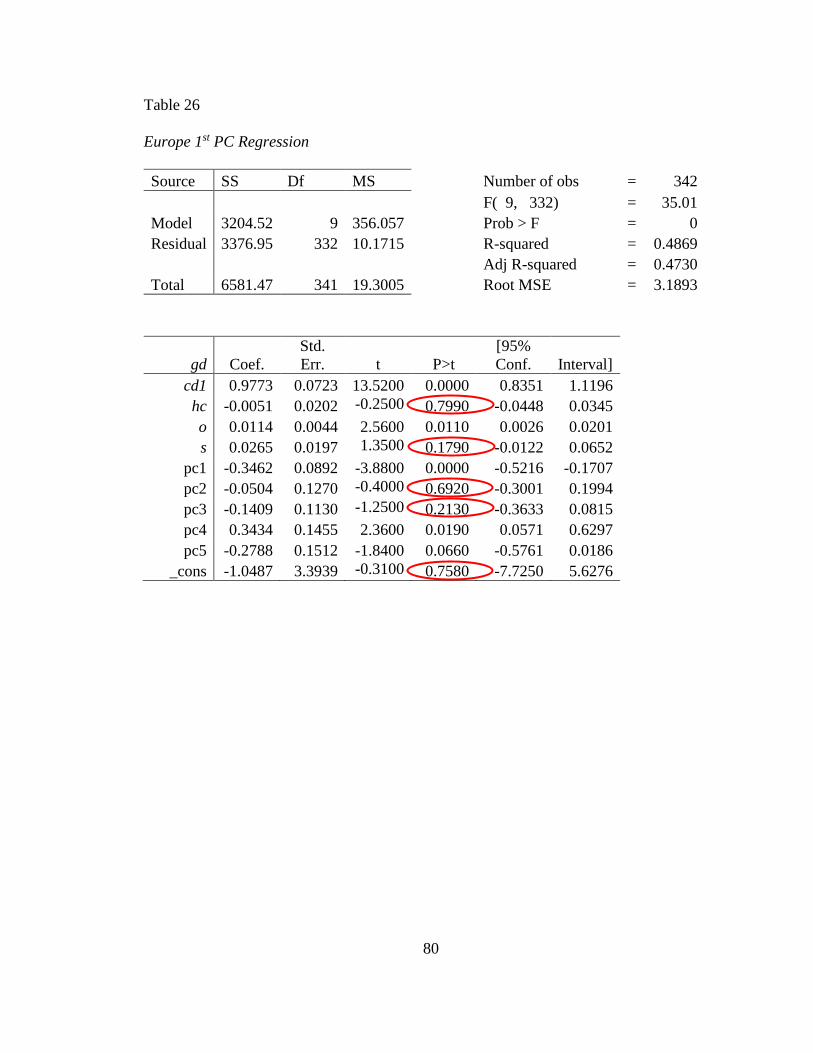
80
Table 26
Europe 1st PC Regression
Source SS Df MS Number of obs = 342
F( 9, 332) = 35.01
Model 3204.52 9 356.057 Prob > F = 0
Residual 3376.95 332 10.1715 R-squared = 0.4869
Adj R-squared = 0.4730
Total 6581.47 341 19.3005 Root MSE = 3.1893
gd Coef.
Std.
Err. t P>t
[95%
Conf. Interval]
cd1 0.9773 0.0723 13.5200 0.0000 0.8351 1.1196
hc -0.0051 0.0202 -0.2500 0.7990 -0.0448 0.0345
o 0.0114 0.0044 2.5600 0.0110 0.0026 0.0201
s 0.0265 0.0197 1.3500 0.1790 -0.0122 0.0652
pc1 -0.3462 0.0892 -3.8800 0.0000 -0.5216 -0.1707
pc2 -0.0504 0.1270 -0.4000 0.6920 -0.3001 0.1994 pc3 -0.1409 0.1130 -1.2500 0.2130 -0.3633 0.0815 pc4 0.3434 0.1455 2.3600 0.0190 0.0571 0.6297 pc5 -0.2788 0.1512 -1.8400 0.0660 -0.5761 0.0186
_cons -1.0487 3.3939 -0.3100 0.7580 -7.7250 5.6276
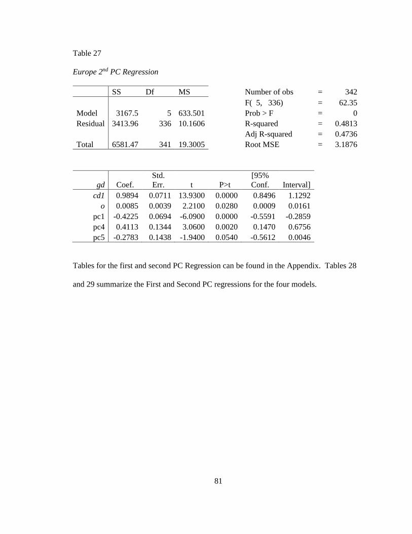
81
Table 27
Europe 2nd PC Regression
SS Df MS Number of obs = 342
F( 5, 336) = 62.35
Model 3167.5 5 633.501 Prob > F = 0
Residual 3413.96 336 10.1606 R-squared = 0.4813
Adj R-squared = 0.4736
Total 6581.47 341 19.3005 Root MSE = 3.1876
gd Coef.
Std.
Err. t P>t
[95%
Conf. Interval] cd1 0.9894 0.0711 13.9300 0.0000 0.8496 1.1292
o 0.0085 0.0039 2.2100 0.0280 0.0009 0.0161 pc1 -0.4225 0.0694 -6.0900 0.0000 -0.5591 -0.2859 pc4 0.4113 0.1344 3.0600 0.0020 0.1470 0.6756 pc5 -0.2783 0.1438 -1.9400 0.0540 -0.5612 0.0046
Tables for the first and second PC Regression can be found in the Appendix. Tables 28
and 29 summarize the First and Second PC regressions for the four models.
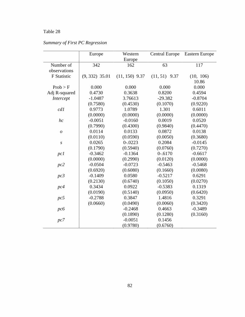
82
Table 28
Summary of First PC Regression
Europe Western
Europe
Central Europe Eastern Europe
Number of
observations
342 162 63 117
F Statistic (9, 332) 35.01 (11, 150) 9.37 (11, 51) 9.37 (10, 106)
10.86
Prob > F 0.000 0.000 0.000 0.000
Adj R-squared 0.4730 0.3638 0.8200 0.4594
Intercept -1.0487
(0.7580)
3.76613
(0.4530)
-29.382
(0.1070)
-0.8704
(0.9220)
cd1 0.9773
(0.0000)
1.0789
(0.0000)
1.301
(0.0000)
0.6011
(0.0000)
hc -0.0051
(0.7990)
-0.0160
(0.4300)
0.0019
(0.9840)
0.0520
(0.4470)
o 0.0114
(0.0110)
0.0133
(0.0590)
0.0872
(0.0050)
0.0138
(0.3680)
s 0.0265
(0.1790)
0-.0223
(0.5940)
0.2084
(0.0760)
-0.0145
(0.7270)
pc1 -0.3462
(0.0000)
-0.1364
(0.2990)
0-.6170
(0.0120)
-0.6617
(0.0000)
pc2 -0.0504
(0.6920)
-0.0723
(0.6080)
-0.5463
(0.1660)
-0.5468
(0.0080)
pc3 -0.1409
(0.2130)
0.0580
(0.6740)
-0.5217
(0.1050)
0.6291
(0.0270)
pc4 0.3434
(0.0190)
0.0922
(0.5140)
-0.5383
(0.0950)
0.1319
(0.6420)
pc5 -0.2788
(0.0660)
0.3847
(0.0490)
1.4816
(0.0060)
0.3291
(0.3420)
pc6 -0.2468
(0.1890)
0.4663
(0.1280)
-0.3489
(0.3160)
pc7 -0.0051
(0.9780)
0.1456
(0.6760)

83
Europe Model 1
Cd1 (investment) and pc1 (depth) are both highly significant. Pc5 (depth
narrow) tests significant also. Added to the model is a marginally significant pc3
(access) at 0.105.
Western Europe Model 2
Control variables hc, o, and s, as well as principal components pc1, pc2, pc3,
pc4, pc6, and pc7 are deleted since they are not statistically significant.
Central Europe Model 3
Three components (pc2, pc6, and pc7) and one control variables (hc) are
eliminated since they did not test significant.
Eastern Europe Model 4
Control variables hc, o, s, and principal components pc2, pc4, and pc6 are deleted
since they are not statistically significant. Following the elimination of the non-
statistically significant variables, a second PC Regression is performed. Table 29
summarizes the four tables found in the Appendix.
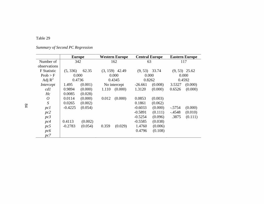
84
Table 29
Summary of Second PC Regression
Europe Western Europe Central Europe Eastern Europe
Number of
observations
342 162 63 117
F Statistic (5, 336) 62.35 (3, 159) 42.49 (9, 53) 33.74 (9, 53) 25.62
Prob > F 0.000 0.000 0.000 0.000
Adj R2 0.4736 0.4345 0.8262 0.4592
Intercept 1.495 (0.001) No intercept -26.661 (0.008) 3.5327 (0.000)
cd1 0.9894 (0.000) 1.110 (0.000) 1.3120 (0.000) 0.6526 (0.000)
Hc 0.0085 (0.028)
O 0.0114 (0.000) 0.012 (0.000) 0.0853 (0.003)
S 0.0265 (0.002) 0.1861 (0.062)
pc1 -0.4225 (0.054) -0.6033 (0.000) -.5754 (0.000)
pc2 -0.5891 (0.111) -.4548 (0.010)
pc3 -0.5254 (0.096) .3875 (0.111)
pc4 0.4113 (0.002) -0.5585 (0.038)
pc5 -0.2783 (0.054) 0.359 (0.029) 1.4760 (0.006)
pc6 0.4796 (0.108)
pc7
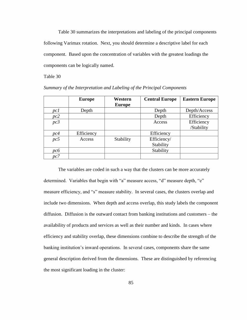
85
Table 30 summarizes the interpretations and labeling of the principal components
following Varimax rotation. Next, you should determine a descriptive label for each
component. Based upon the concentration of variables with the greatest loadings the
components can be logically named.
Table 30
Summary of the Interpretation and Labeling of the Principal Components
Europe Western
Europe
Central Europe Eastern Europe
pc1 Depth Depth Depth/Access
pc2 Depth Efficiency
pc3 Access Efficiency
/Stability
pc4 Efficiency Efficiency
pc5 Access Stability Efficiency/
Stability
pc6 Stability
pc7
The variables are coded in such a way that the clusters can be more accurately
determined. Variables that begin with “a” measure access, “d” measure depth, “e”
measure efficiency, and “s” measure stability. In several cases, the clusters overlap and
include two dimensions. When depth and access overlap, this study labels the component
diffusion. Diffusion is the outward contact from banking institutions and customers – the
availability of products and services as well as their number and kinds. In cases where
efficiency and stability overlap, these dimensions combine to describe the strength of the
banking institution’s inward operations. In several cases, components share the same
general description derived from the dimensions. These are distinguished by referencing
the most significant loading in the cluster:

86
a) Europe has three clusters – depth, efficiency, and access;
b) Western Europe has one cluster – stability;
c) Central Europe has six clusters – depth of credit, depth of deposits, access,
d) efficiency, operations, and stability; and,
e) Eastern Europe has three clusters – diffusion, efficiency, and operations.
The model should be specified with significant variables and components. From
the principal component labels in Table 33 and the coefficients in Table 32 four models
are specified:
Europe Model 1
gde = 1.495 + 0.9894capital + 0.0085technology + 0.0114openness
+ 0.0265government spending - 0.4225depth + 0.4113efficiency
- 0.2783access + εe (5)
Western Europe Model 2
gdw = 1.110capital + 0.012openness + 0.359stability + εw (6)
Central Europe Model 3
gdc = -26.661 + 1.3120capital + 0.0853openness
+ 0.1861government spending - 0.6033depth credit
- 0.5891depth deposits - 0.5254access - 0.5585efficiency

87
+ 1.4760operations + 0 .4796stability + εc (7)
Eastern Europe Model 4
gde = 3.5327 + 0.6551capital - 0.5754diffusion - 0.4548efficiency
+ 0.3875operations + εe (8)

88
CHAPTER V – CONCLUSIONS
This chapter summarizes the effects of banking development on economic growth
in three regions of Europe. These effects have implications in additional research in
growth theory and development policy. A discussion of the specific contributions to the
literature provided by this study follows. Next, the limitations of this research are noted.
Finally, recommendations for further research are offered.
Effects of Banking Development on Economic Growth
Correlation
Europe, as an aggregate, and three regions of Europe are examined. Each region
is characterized by a different level of economic development and is tested for the
supply-following hypothesis. The results demonstrate that banking development has a
strong correlation with economic growth. Four OLS models test this correlation and find
a general association, though the degree of the correlation varies from model to model.
The Europe, Western Europe, and Eastern Europe models share similar Adj. R2s (0.43 to
0.47), but there is a significant outlier with Central Europe (0.81). The p values for the F-
statistics in all four models is < 0.000. We conclude the tests support the hypothesis that
there is correlation between the independent variables and economic growth.
Control Variables
Based on the literature, OLS models utilize four control variables, though not
always at the same time. They are investment, human capital, openness and government
spending. This study introduces all four of the variables to the regression equation. The
tests demonstrate that investment capital is the single most important contributor. All

89
four regressions indicate this control variable is highly significant (p < 0.000). Another
control variable, openness, tested well also. Its results are significant or highly significant
in three models, Europe (p < 0.028), Western Europe (p < 0.000) and Central Europe (p <
0.008). Openness, as measured by total trade, is statistically significance in the more
developed economies of Central and Western Europe, as well as Europe in the aggregate.
Future research should include these two variables as controls.
The remaining control variables are determined to be inconsequential.
Government spending proved to be significant in only one model, Central Europe.
Human capital, as measured by percent of the population with secondary education, was
found not to be statistically significant for any of the models.
Independent Variables/Components
The World Bank’s guidance in broadening the definition of development led this
study to increase the number of proxies for access, depth, efficiency, and solvency
significantly. With twenty-one variables multicollinearity issues is of concern. Recent
literature provides guidance in the use of principal components, an orthogonal
transformation tool which overcomes the problems presented by multicollinearity.
Through this method, twenty-one variables are transformed into five to seven
components that retain at least 72% of the information of the variances.
As the components are deconstructed into their most significant eigenvectors,
they reflect different variable weightings, and can more thoroughly describe the
correlation than just the four generalized dimensions. Central and Eastern Europe’s
greatest association are from depth of products and services available to customers.
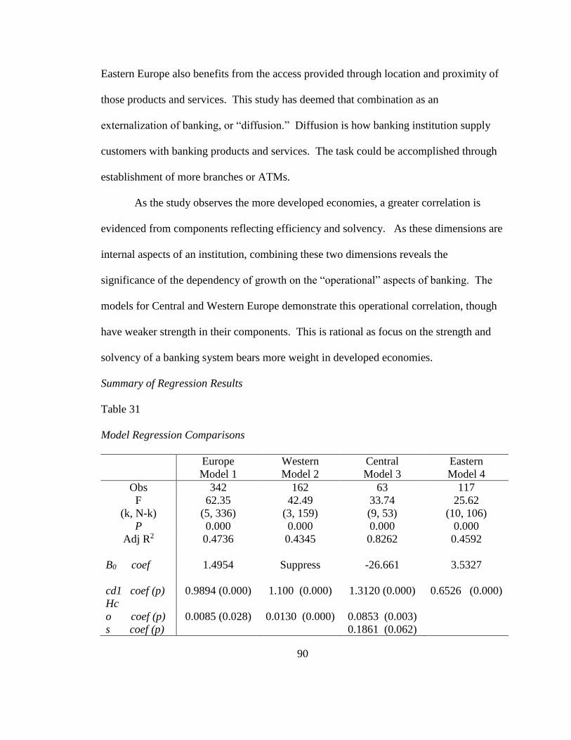
90
Eastern Europe also benefits from the access provided through location and proximity of
those products and services. This study has deemed that combination as an
externalization of banking, or “diffusion.” Diffusion is how banking institution supply
customers with banking products and services. The task could be accomplished through
establishment of more branches or ATMs.
As the study observes the more developed economies, a greater correlation is
evidenced from components reflecting efficiency and solvency. As these dimensions are
internal aspects of an institution, combining these two dimensions reveals the
significance of the dependency of growth on the “operational” aspects of banking. The
models for Central and Western Europe demonstrate this operational correlation, though
have weaker strength in their components. This is rational as focus on the strength and
solvency of a banking system bears more weight in developed economies.
Summary of Regression Results
Table 31
Model Regression Comparisons
Europe
Model 1
Western
Model 2
Central
Model 3
Eastern
Model 4
Obs 342 162 63 117
F
(k, N-k)
62.35
(5, 336)
42.49
(3, 159)
33.74
(9, 53)
25.62
(10, 106)
P 0.000 0.000 0.000 0.000
Adj R2 0.4736 0.4345
0.8262
0.4592
B0 coef 1.4954 Suppress -26.661
3.5327
cd1 coef (p) 0.9894 (0.000) 1.100 (0.000) 1.3120 (0.000) 0.6526 (0.000)
Hc
o coef (p) 0.0085 (0.028) 0.0130 (0.000) 0.0853 (0.003)
s coef (p) 0.1861 (0.062)
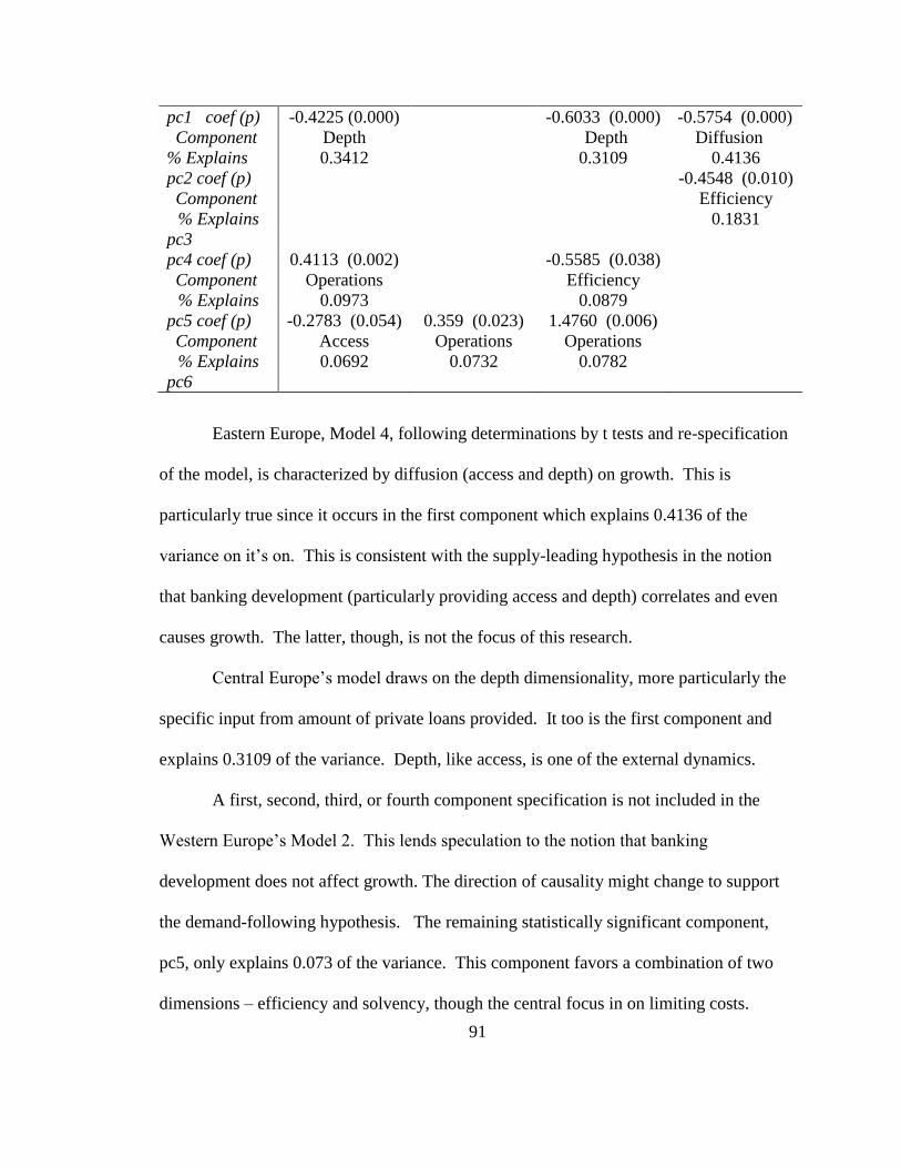
91
pc1 coef (p)
Component
% Explains
-0.4225 (0.000)
Depth
0.3412
-0.6033 (0.000)
Depth
0.3109
-0.5754 (0.000)
Diffusion
0.4136
pc2 coef (p)
Component
% Explains
-0.4548 (0.010)
Efficiency
0.1831
pc3
pc4 coef (p)
Component
% Explains
0.4113 (0.002)
Operations
0.0973
-0.5585 (0.038)
Efficiency
0.0879
pc5 coef (p)
Component
% Explains
-0.2783 (0.054)
Access
0.0692
0.359 (0.023)
Operations
0.0732
1.4760 (0.006)
Operations
0.0782
pc6
Eastern Europe, Model 4, following determinations by t tests and re-specification
of the model, is characterized by diffusion (access and depth) on growth. This is
particularly true since it occurs in the first component which explains 0.4136 of the
variance on it’s on. This is consistent with the supply-leading hypothesis in the notion
that banking development (particularly providing access and depth) correlates and even
causes growth. The latter, though, is not the focus of this research.
Central Europe’s model draws on the depth dimensionality, more particularly the
specific input from amount of private loans provided. It too is the first component and
explains 0.3109 of the variance. Depth, like access, is one of the external dynamics.
A first, second, third, or fourth component specification is not included in the
Western Europe’s Model 2. This lends speculation to the notion that banking
development does not affect growth. The direction of causality might change to support
the demand-following hypothesis. The remaining statistically significant component,
pc5, only explains 0.073 of the variance. This component favors a combination of two
dimensions – efficiency and solvency, though the central focus in on limiting costs.

92
Comparison
The four models vary in their number of qualified components, component
loadings, and statistical significance. Table 32 demonstrates the summary of the number
of principal components that are significant out of the original model’s qualified
components.
Table 32
Summary of Significant Principal Components
Model Europe Western
Europe
Central
Europe
Eastern
Europe
Significant
of Qualified
3
of 5
1
of 7
3
of 5
2
Of 5
One deduction from the analysis is that components have the strongest impact upon
Central Europe first, then Eastern Europe, and finally Western Europe. This is consistent
with the progressive thought that the less developed economies enjoy the greatest benefit
from banking development than the more developed economies.
Theory
The supply-leading hypothesis, particularly as banking development provides
banking products and services with increasing availability by number and proximity, fits
rationally with this finding. Conversely, the lack of power of these components in
developed economies provide less support for the supply-leading hypothesis and
increases possibility for the demand- following hypothesis. This can be generalized as
less developed economies have a greater dependence on banking development to
stimulate growth and the developed economies create demand for more and newer

93
banking products and services. This latter part is the subject of additional causality
research.
Contributions to Literature
World Bank (2005) introduced four dimensions to describe financial/ banking
development – access, depth, efficiency, and stability. Each of these reflect different
aspects of banking and together provide a better description of development. This more
thorough measurement has not been fully utilized in testing the supply-leading hypothesis
in the literature. This study begins with those four dimensions and contributes three
additional alternatives:
a) introduce a significant number of additional banking metrics representing
each of the four dimensions:
b) orthogonal transformation of the metrics into principal components analysis;
and,
c) use the components to redefine the merged dimensions and provide a newer
reflection.
When the dimensions merge through PCA, new aspects surface. Two examples
include:
1) The access and depth combination that results in an outward, ”diffusion”
reflection; and,
2) The efficiency and stability merger that results in an internalized reflection
termed “operations.”

94
The first example speaks to how well banking institutions diffuse themselves into the
economy, reflected by the number of product and services offered and utilized as well as
the proximity to the customer. The second speaks to the strength of the institution, its
profitable nature, and capital foundation.
This study has contributed to the literature in five ways: understanding of banking
development; addition of proxies; adoption of PCA; banking to growth models; and
geographic region differences.
Utilized a More Thorough Understanding of “Banking Development;”
By an understanding from World Bank contributors, financial development has
been pressed to be further defined with four dimensions. These dimensions – access,
depth, efficiency, and solvency – provide a more thorough expression of the dynamics
within development. It is expected that by incorporating this refined explanation into a
model, a clearer correlation between specific metrics of development can be causality
tested.
Incorporated a Significantly Larger Number of Proxies to Fulfill the Thoroughness of
Model Specification;
This study has selected four to six different macro and micro metrics to quantify
the four dimensions. While previous studies have typically used four or less independent
variables, this study expanded the list to twenty-one. These proxies quantify the
dynamics of development in a more thorough manner.
Adopted Principal Component Analysis in the Model Building Framework;

95
For the two reasons of multicollinearity and complexity, principal component
analysis is used to create a series of indexes. The proxies are orthogonally transformed to
create a potential predictor. Each of the components favor some weighted dimension or
combination of dimensions that can further express dynamics.
Develop Models that are Banking to Growth Orientation
Banking development is posited to cause economic growth. The derived
components reflected in this study are thought to demonstrate that relationship. The four
models that are specified share similarities in the dynamics of the expressions. Though
not tested, the differences are expected to be found in the association with growth.
Different aspects of development have varying degrees of association. By dividing
Europe into three sub-regions, these differences may be heightened and measured.
Focused on a Specific Geographical Region
The growth rates regressed on control variables and components to determine
specifications for each of the four models – Europe, Western Europe, Central Europe, and
Eastern Europe. Each model is specified with components having similar and or different
expressions of underlying dimensions. This is expected as the different regions reflect
different growth rates.
Limitations of This Study
There are four principal limitations in this study: depth of the data set, types of
proxies, determination of causality, and explanation of negative coefficients.

96
Data Set is Limited
Accessibility, depth, efficiency and stability have a number of ways to be
measured. Though the micro measurements for the banking industry has expanded
significantly since 1992, the depth for each of those metrics has been inconsistent. There
are variables that would better suit to express the associative relationship and the causal
power, but the period for which the data has been recorded and the breath of countries
reporting is limited.
Improve Types of Proxies
The number of banking metrics is continuing to expand by the World Bank,
United States, and European Central Bank reporting requirements. As the institutions
harmonize their information requirements and data sets, more specific asset and liability
classes, as well as numerous kinds of banking services, can be captured. This adds to the
thoroughness of measuring banking development.
Determination of Causality
Based upon the Adj. R2, each of the four models indicates the associative power
of banking development with economic growth. Different growth rates for the regions
associated with varying dynamics. This study does not test for direction of causality.
This is the greatest unresolved issue with this study.
Explanation of the Negative Coefficients
The goal of regression using the components is to provide a better understanding
of the relationships of the underlying structures of the data and growth. These structures
are formed from the loadings of the variables that go to form the components. If the

97
coefficients and loadings for the components in the model have a meaningful
interpretations, then the goal is achieved.
Interpretation of the principal components is based on the variables that are most
strongly correlated with each component. Interpretations are clearer when the
coefficients are positive. However, in each of this study’s models, there are significant
components with negative coefficients. As these coefficients reflect the signs of the
loadings, interpretations are not always clear or may be counter-intuitive (Jolliffe, 1982).
Further Study and Research
There are three principal directions the research could proceed in investigating the
supply-leading hypothesis: direction of causality, improvement in selection of proxies,
and cross country effects.
Short and Long Run Direction of Causality
This study only reviews the correlation between banking development and
economic growth. As a result, causality cannot be inferred. Incorporation of statistical
tools like panel vector autoregression may provide this next step in the direction of the
causality - even discriminating between lesser developed and developed economies.
Improved Depth and Selection of Proxies
The banking data sets will continue to deepen both by backfilling from secondary
sources as well as the additions of years going forward. New metrics can refine the
meaning of the four dimensions of development proffered by the World Bank - access,
depth, efficiency, and stability. The richness of the description of development and the

98
discovery of new causalities from the created proxies could open opportunities to
establish effective policies.
Cross Country Effects
Commercial banking in evolved economies tend to seek opportunities outside of
their domiciled countries. They are often the first to branch across borders to seek
additional opportunities for their own growth. As a result, this could provide a stimulus
to lesser developed economies. The network of Western European banks branching or
merging with banks in Central and Eastern Europe is similar to a foreign direct
investment. That dynamic has not been analyzed in the literature.
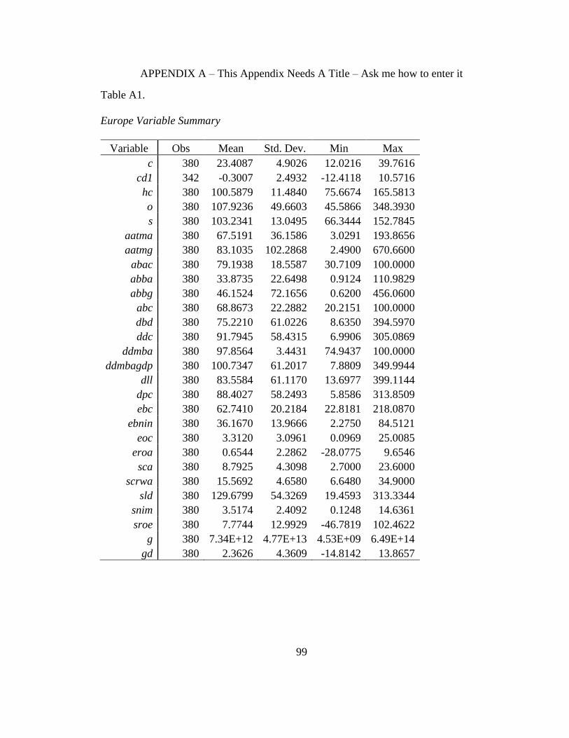
99
APPENDIX A – This Appendix Needs A Title – Ask me how to enter it
Table A1.
Europe Variable Summary
Variable Obs Mean Std. Dev. Min Max
c 380 23.4087 4.9026 12.0216 39.7616
cd1 342 -0.3007 2.4932 -12.4118 10.5716
hc 380 100.5879 11.4840 75.6674 165.5813
o 380 107.9236 49.6603 45.5866 348.3930
s 380 103.2341 13.0495 66.3444 152.7845
aatma 380 67.5191 36.1586 3.0291 193.8656
aatmg 380 83.1035 102.2868 2.4900 670.6600
abac 380 79.1938 18.5587 30.7109 100.0000
abba 380 33.8735 22.6498 0.9124 110.9829
abbg 380 46.1524 72.1656 0.6200 456.0600
abc 380 68.8673 22.2882 20.2151 100.0000
dbd 380 75.2210 61.0226 8.6350 394.5970
ddc 380 91.7945 58.4315 6.9906 305.0869
ddmba 380 97.8564 3.4431 74.9437 100.0000
ddmbagdp 380 100.7347 61.2017 7.8809 349.9944
dll 380 83.5584 61.1170 13.6977 399.1144
dpc 380 88.4027 58.2493 5.8586 313.8509
ebc 380 62.7410 20.2184 22.8181 218.0870
ebnin 380 36.1670 13.9666 2.2750 84.5121
eoc 380 3.3120 3.0961 0.0969 25.0085
eroa 380 0.6544 2.2862 -28.0775 9.6546
sca 380 8.7925 4.3098 2.7000 23.6000
scrwa 380 15.5692 4.6580 6.6480 34.9000
sld 380 129.6799 54.3269 19.4593 313.3344
snim 380 3.5174 2.4092 0.1248 14.6361
sroe 380 7.7744 12.9929 -46.7819 102.4622
g 380 7.34E+12 4.77E+13 4.53E+09 6.49E+14
gd 380 2.3626 4.3609 -14.8142 13.8657
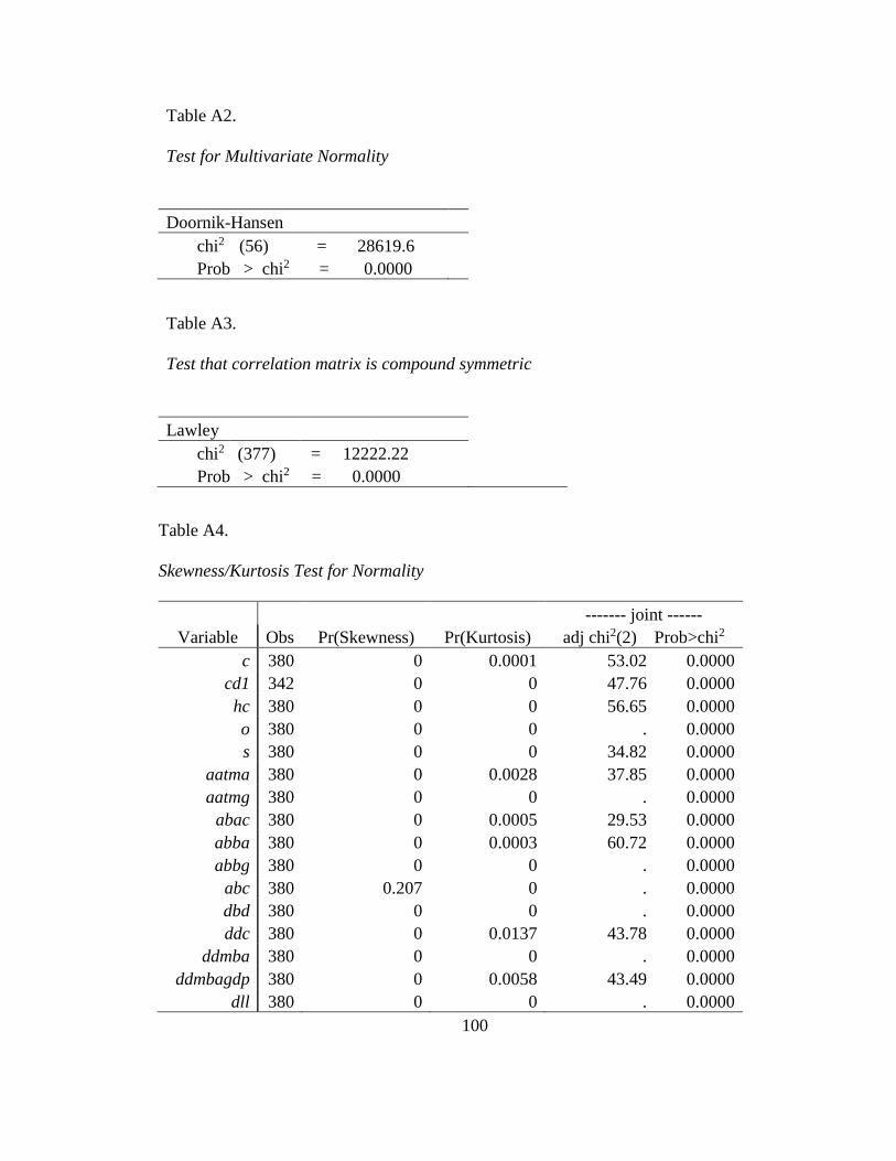
100
Table A2.
Test for Multivariate Normality
Doornik-Hansen chi2 (56) = 28619.6 Prob > chi2 = 0.0000
Table A3.
Test that correlation matrix is compound symmetric
Lawley chi2 (377) = 12222.22 Prob > chi2 = 0.0000
Table A4.
Skewness/Kurtosis Test for Normality
------- joint ------
Variable Obs Pr(Skewness) Pr(Kurtosis) adj chi2(2) Prob>chi2
c 380 0 0.0001 53.02 0.0000
cd1 342 0 0 47.76 0.0000
hc 380 0 0 56.65 0.0000
o 380 0 0 . 0.0000
s 380 0 0 34.82 0.0000
aatma 380 0 0.0028 37.85 0.0000
aatmg 380 0 0 . 0.0000
abac 380 0 0.0005 29.53 0.0000
abba 380 0 0.0003 60.72 0.0000
abbg 380 0 0 . 0.0000
abc 380 0.207 0 . 0.0000
dbd 380 0 0 . 0.0000
ddc 380 0 0.0137 43.78 0.0000
ddmba 380 0 0 . 0.0000
ddmbagdp 380 0 0.0058 43.49 0.0000
dll 380 0 0 . 0.0000
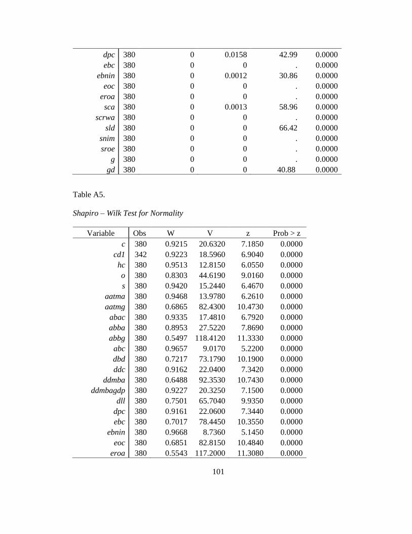
101
dpc 380 0 0.0158 42.99 0.0000
ebc 380 0 0 . 0.0000
ebnin 380 0 0.0012 30.86 0.0000
eoc 380 0 0 . 0.0000
eroa 380 0 0 . 0.0000
sca 380 0 0.0013 58.96 0.0000
scrwa 380 0 0 . 0.0000
sld 380 0 0 66.42 0.0000
snim 380 0 0 . 0.0000
sroe 380 0 0 . 0.0000
g 380 0 0 . 0.0000
gd 380 0 0 40.88 0.0000
Table A5.
Shapiro – Wilk Test for Normality
Variable Obs W V z Prob > z
c 380 0.9215 20.6320 7.1850 0.0000
cd1 342 0.9223 18.5960 6.9040 0.0000
hc 380 0.9513 12.8150 6.0550 0.0000
o 380 0.8303 44.6190 9.0160 0.0000
s 380 0.9420 15.2440 6.4670 0.0000
aatma 380 0.9468 13.9780 6.2610 0.0000
aatmg 380 0.6865 82.4300 10.4730 0.0000
abac 380 0.9335 17.4810 6.7920 0.0000
abba 380 0.8953 27.5220 7.8690 0.0000
abbg 380 0.5497 118.4120 11.3330 0.0000
abc 380 0.9657 9.0170 5.2200 0.0000
dbd 380 0.7217 73.1790 10.1900 0.0000
ddc 380 0.9162 22.0400 7.3420 0.0000
ddmba 380 0.6488 92.3530 10.7430 0.0000
ddmbagdp 380 0.9227 20.3250 7.1500 0.0000
dll 380 0.7501 65.7040 9.9350 0.0000
dpc 380 0.9161 22.0600 7.3440 0.0000
ebc 380 0.7017 78.4450 10.3550 0.0000
ebnin 380 0.9668 8.7360 5.1450 0.0000
eoc 380 0.6851 82.8150 10.4840 0.0000
eroa 380 0.5543 117.2000 11.3080 0.0000
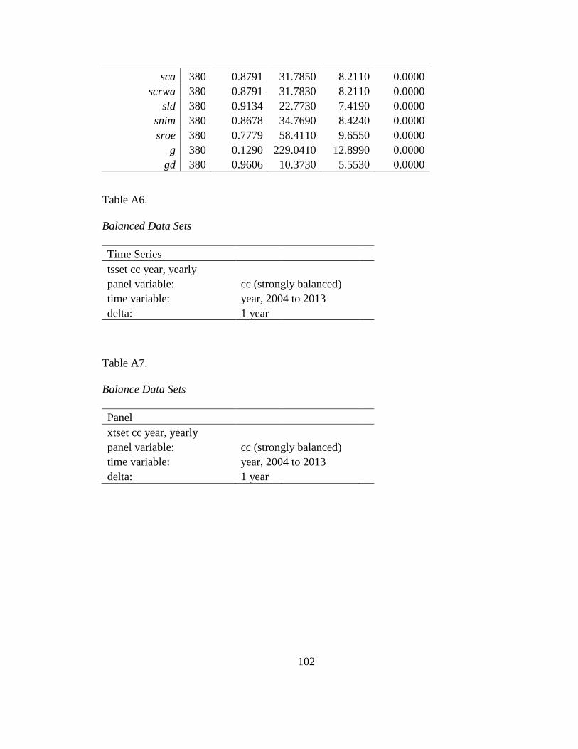
102
sca 380 0.8791 31.7850 8.2110 0.0000
scrwa 380 0.8791 31.7830 8.2110 0.0000
sld 380 0.9134 22.7730 7.4190 0.0000
snim 380 0.8678 34.7690 8.4240 0.0000
sroe 380 0.7779 58.4110 9.6550 0.0000
g 380 0.1290 229.0410 12.8990 0.0000
gd 380 0.9606 10.3730 5.5530 0.0000
Table A6.
Balanced Data Sets
Time Series
tsset cc year, yearly panel variable: cc (strongly balanced)
time variable: year, 2004 to 2013 delta: 1 year
Table A7.
Balance Data Sets
Panel
xtset cc year, yearly panel variable: cc (strongly balanced)
time variable: year, 2004 to 2013 delta: 1 year

103
Table A8.
Unit Root Tests for Control and Independent Variables
Levin-Lin-Chu unit-root test for cd1
Ho: Panels contain unit roots Number of panels = 38 Ha: Panels are stationary Number of periods = 9 Statistic p-value Unadjusted t -18.9366 Adjusted t* -14.1921 0.0000
Levin-Lin-Chu unit-root test for hc
Ho: Panels contain unit roots Number of panels = 38 Ha: Panels are stationary Number of periods = 10 Statistic p-value Unadjusted t -5.6825 Adjusted t* 1.3554 0.9124
Levin-Lin-Chu unit-root test for o
Ho: Panels contain unit roots Number of panels = 38 Ha: Panels are stationary Number of periods = 10 Statistic p-value Unadjusted t -11.5156 Adjusted t* -6.8388 0.0000
Levin-Lin-Chu unit-root test for s
Ho: Panels contain unit roots Number of panels = 38
Ha: Panels are stationary Number of periods = 10
Statistic p-value Unadjusted t -7.7604

104
Levin-Lin-Chu unit-root test for abba
Ho: Panels contain unit roots Number of panels = 38
Ha: Panels are stationary Number of periods = 10
Statistic p-value Unadjusted t -7.1944 Adjusted t* -4.0112 0.0000
Levin-Lin-Chu unit-root test for abbg
Ho: Panels contain unit roots Number of panels = 38
Ha: Panels are stationary Number of periods = 10
Statistic p-value
Adjusted t* -3.1507 0.0008
Levin-Lin-Chu unit-root test for aatma
Ho: Panels contain unit roots Number of panels = 38
Ha: Panels are stationary Number of periods = 10
Statistic p-value Unadjusted t -31.9657 Adjusted t* -34.0419 0.0000
Levin-Lin-Chu unit-root test for aatmg
Ho: Panels contain unit roots Number of panels = 38
Ha: Panels are stationary Number of periods = 10
Statistic p-value Unadjusted t -15.3781 Adjusted t* -14.6710 0.0000
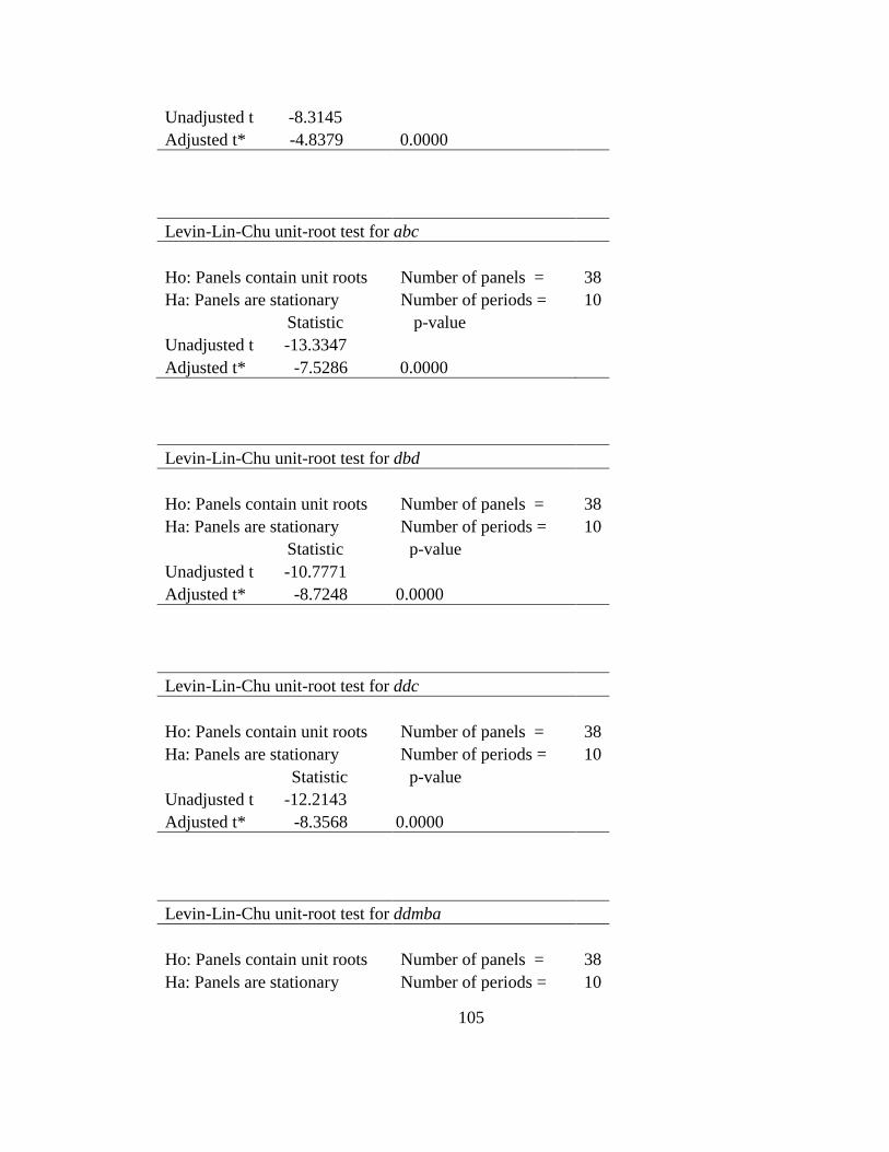
105
Unadjusted t -8.3145 Adjusted t* -4.8379 0.0000
Levin-Lin-Chu unit-root test for abc
Ho: Panels contain unit roots Number of panels = 38
Ha: Panels are stationary Number of periods = 10
Statistic p-value Unadjusted t -13.3347 Adjusted t* -7.5286 0.0000
Levin-Lin-Chu unit-root test for dbd
Ho: Panels contain unit roots Number of panels = 38
Ha: Panels are stationary Number of periods = 10
Statistic p-value Unadjusted t -10.7771 Adjusted t* -8.7248 0.0000
Levin-Lin-Chu unit-root test for ddc
Ho: Panels contain unit roots Number of panels = 38
Ha: Panels are stationary Number of periods = 10
Statistic p-value Unadjusted t -12.2143 Adjusted t* -8.3568 0.0000
Levin-Lin-Chu unit-root test for ddmba
Ho: Panels contain unit roots Number of panels = 38
Ha: Panels are stationary Number of periods = 10
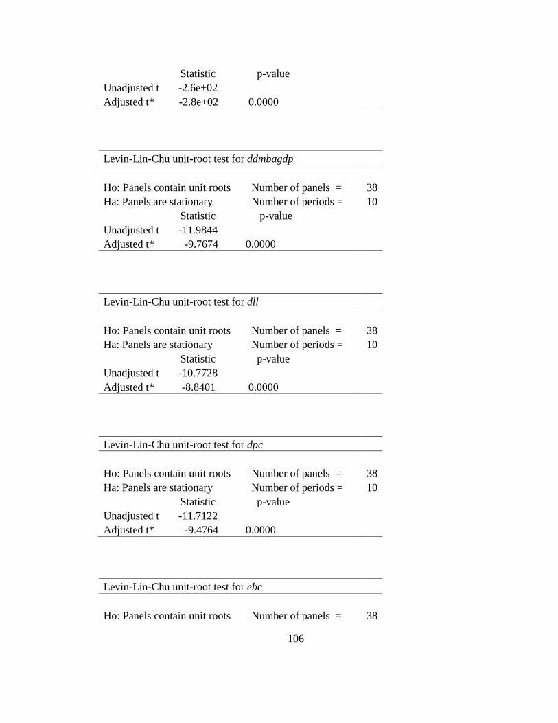
106
Statistic p-value Unadjusted t -2.6e+02 Adjusted t* -2.8e+02 0.0000
Levin-Lin-Chu unit-root test for ddmbagdp
Ho: Panels contain unit roots Number of panels = 38
Ha: Panels are stationary Number of periods = 10
Statistic p-value Unadjusted t -11.9844 Adjusted t* -9.7674 0.0000
Levin-Lin-Chu unit-root test for dll
Ho: Panels contain unit roots Number of panels = 38
Ha: Panels are stationary Number of periods = 10
Statistic p-value Unadjusted t -10.7728 Adjusted t* -8.8401 0.0000
Levin-Lin-Chu unit-root test for dpc
Ho: Panels contain unit roots Number of panels = 38
Ha: Panels are stationary Number of periods = 10
Statistic p-value Unadjusted t -11.7122 Adjusted t* -9.4764 0.0000
Levin-Lin-Chu unit-root test for ebc
Ho: Panels contain unit roots Number of panels = 38
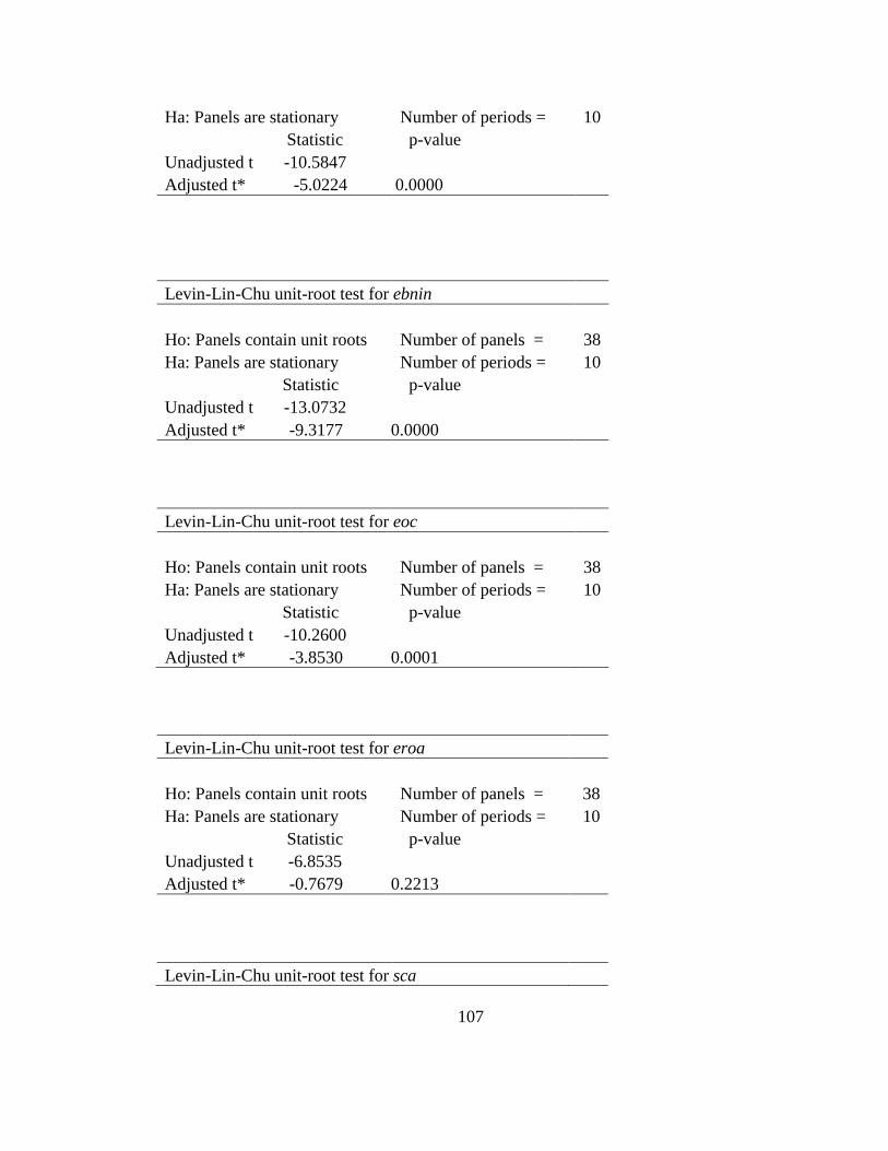
107
Ha: Panels are stationary Number of periods = 10
Statistic p-value Unadjusted t -10.5847 Adjusted t* -5.0224 0.0000
Levin-Lin-Chu unit-root test for ebnin
Ho: Panels contain unit roots Number of panels = 38
Ha: Panels are stationary Number of periods = 10
Statistic p-value Unadjusted t -13.0732 Adjusted t* -9.3177 0.0000
Levin-Lin-Chu unit-root test for eoc
Ho: Panels contain unit roots Number of panels = 38
Ha: Panels are stationary Number of periods = 10
Statistic p-value Unadjusted t -10.2600 Adjusted t* -3.8530 0.0001
Levin-Lin-Chu unit-root test for eroa
Ho: Panels contain unit roots Number of panels = 38
Ha: Panels are stationary Number of periods = 10
Statistic p-value Unadjusted t -6.8535 Adjusted t* -0.7679 0.2213
Levin-Lin-Chu unit-root test for sca
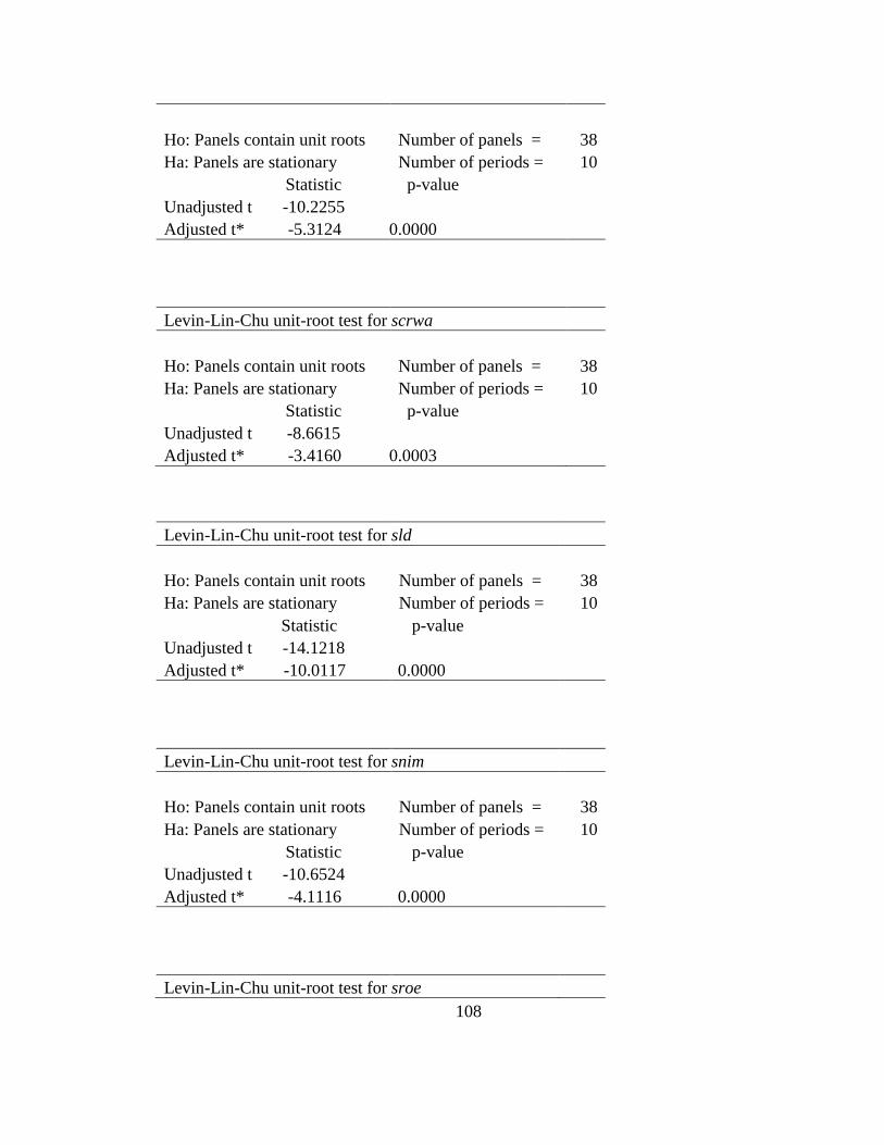
108
Ho: Panels contain unit roots Number of panels = 38
Ha: Panels are stationary Number of periods = 10
Statistic p-value Unadjusted t -10.2255 Adjusted t* -5.3124 0.0000
Levin-Lin-Chu unit-root test for scrwa
Ho: Panels contain unit roots Number of panels = 38
Ha: Panels are stationary Number of periods = 10
Statistic p-value Unadjusted t -8.6615 Adjusted t* -3.4160 0.0003
Levin-Lin-Chu unit-root test for sld
Ho: Panels contain unit roots Number of panels = 38
Ha: Panels are stationary Number of periods = 10
Statistic p-value Unadjusted t -14.1218 Adjusted t* -10.0117 0.0000
Levin-Lin-Chu unit-root test for snim
Ho: Panels contain unit roots Number of panels = 38
Ha: Panels are stationary Number of periods = 10
Statistic p-value Unadjusted t -10.6524 Adjusted t* -4.1116 0.0000
Levin-Lin-Chu unit-root test for sroe
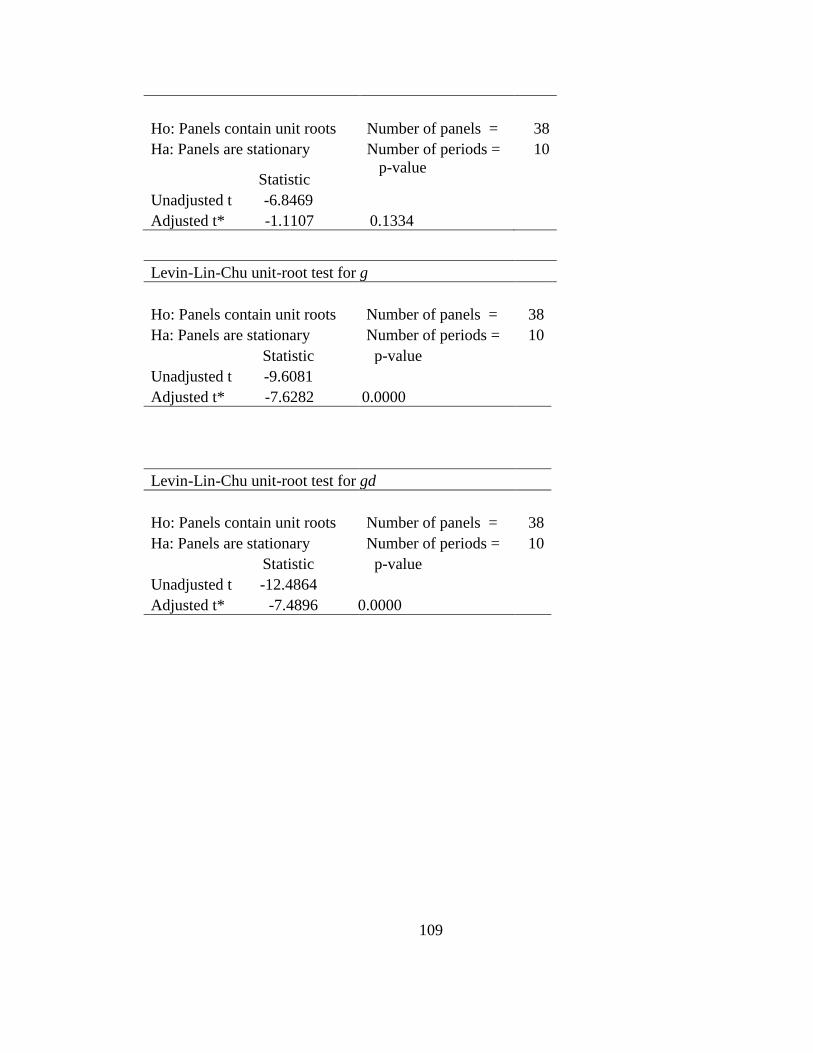
109
Ho: Panels contain unit roots Number of panels = 38
Ha: Panels are stationary Number of periods = 10
Statistic p-value
Unadjusted t -6.8469 Adjusted t* -1.1107 0.1334
Levin-Lin-Chu unit-root test for g
Ho: Panels contain unit roots Number of panels = 38
Ha: Panels are stationary Number of periods = 10
Statistic p-value
Unadjusted t -9.6081
Adjusted t* -7.6282 0.0000
Levin-Lin-Chu unit-root test for gd
Ho: Panels contain unit roots Number of panels = 38
Ha: Panels are stationary Number of periods = 10
Statistic p-value
Unadjusted t -12.4864
Adjusted t* -7.4896 0.0000
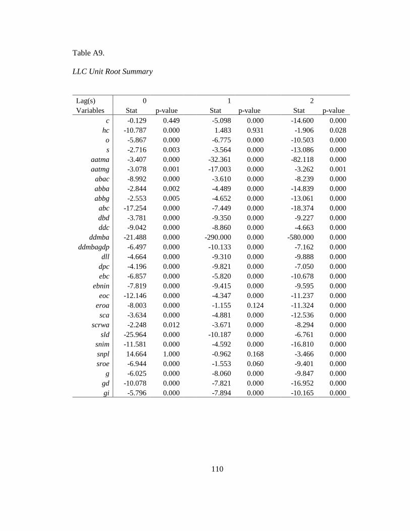
110
Table A9.
LLC Unit Root Summary
Lag(s) 0 1 2
Variables Stat p-value Stat p-value Stat p-value
c -0.129 0.449 -5.098 0.000 -14.600 0.000
hc -10.787 0.000 1.483 0.931 -1.906 0.028
o -5.867 0.000 -6.775 0.000 -10.503 0.000
s -2.716 0.003 -3.564 0.000 -13.086 0.000
aatma -3.407 0.000 -32.361 0.000 -82.118 0.000
aatmg -3.078 0.001 -17.003 0.000 -3.262 0.001
abac -8.992 0.000 -3.610 0.000 -8.239 0.000
abba -2.844 0.002 -4.489 0.000 -14.839 0.000
abbg -2.553 0.005 -4.652 0.000 -13.061 0.000
abc -17.254 0.000 -7.449 0.000 -18.374 0.000
dbd -3.781 0.000 -9.350 0.000 -9.227 0.000
ddc -9.042 0.000 -8.860 0.000 -4.663 0.000
ddmba -21.488 0.000 -290.000 0.000 -580.000 0.000
ddmbagdp -6.497 0.000 -10.133 0.000 -7.162 0.000
dll -4.664 0.000 -9.310 0.000 -9.888 0.000
dpc -4.196 0.000 -9.821 0.000 -7.050 0.000
ebc -6.857 0.000 -5.820 0.000 -10.678 0.000
ebnin -7.819 0.000 -9.415 0.000 -9.595 0.000
eoc -12.146 0.000 -4.347 0.000 -11.237 0.000
eroa -8.003 0.000 -1.155 0.124 -11.324 0.000
sca -3.634 0.000 -4.881 0.000 -12.536 0.000
scrwa -2.248 0.012 -3.671 0.000 -8.294 0.000
sld -25.964 0.000 -10.187 0.000 -6.761 0.000
snim -11.581 0.000 -4.592 0.000 -16.810 0.000
snpl 14.664 1.000 -0.962 0.168 -3.466 0.000
sroe -6.944 0.000 -1.553 0.060 -9.401 0.000
g -6.025 0.000 -8.060 0.000 -9.847 0.000
gd -10.078 0.000 -7.821 0.000 -16.952 0.000
gi -5.796 0.000 -7.894 0.000 -10.165 0.000
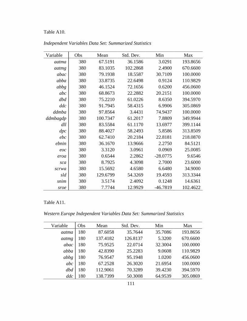
111
Table A10.
Independent Variables Data Set: Summarized Statistics
Variable Obs Mean Std. Dev. Min Max
aatma 380 67.5191 36.1586 3.0291 193.8656
aatmg 380 83.1035 102.2868 2.4900 670.6600
abac 380 79.1938 18.5587 30.7109 100.0000
abba 380 33.8735 22.6498 0.9124 110.9829
abbg 380 46.1524 72.1656 0.6200 456.0600
abc 380 68.8673 22.2882 20.2151 100.0000
dbd 380 75.2210 61.0226 8.6350 394.5970
ddc 380 91.7945 58.4315 6.9906 305.0869
ddmba 380 97.8564 3.4431 74.9437 100.0000
ddmbagdp 380 100.7347 61.2017 7.8809 349.9944
dll 380 83.5584 61.1170 13.6977 399.1144
dpc 380 88.4027 58.2493 5.8586 313.8509
ebc 380 62.7410 20.2184 22.8181 218.0870
ebnin 380 36.1670 13.9666 2.2750 84.5121
eoc 380 3.3120 3.0961 0.0969 25.0085
eroa 380 0.6544 2.2862 -28.0775 9.6546
sca 380 8.7925 4.3098 2.7000 23.6000
scrwa 380 15.5692 4.6580 6.6480 34.9000
sld 380 129.6799 54.3269 19.4593 313.3344
snim 380 3.5174 2.4092 0.1248 14.6361
sroe 380 7.7744 12.9929 -46.7819 102.4622
Table A11.
Western Europe Independent Variables Data Set: Summarized Statistics
Variable Obs Mean Std. Dev. Min Max
aatma 180 87.6058 35.7644 35.7086 193.8656
aatmg 180 137.4182 126.8137 5.3200 670.6600
abac 180 75.9525 22.0714 32.3004 100.0000
abba 180 42.8390 25.2283 9.0608 110.9829
abbg 180 76.9547 95.1948 1.0200 456.0600
abc 180 67.2528 26.3020 21.6954 100.0000
dbd 180 112.9061 70.3289 39.4230 394.5970
ddc 180 138.7399 50.3008 64.9539 305.0869
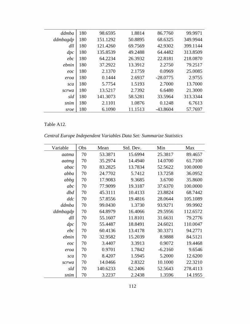
112
ddmba 180 98.6595 1.8814 86.7760 99.9971
ddmbagdp 180 151.1292 50.8895 68.6325 349.9944
dll 180 121.4260 69.7569 42.9302 399.1144
dpc 180 135.8539 49.2488 64.4482 313.8509
ebc 180 64.2234 26.3932 22.8181 218.0870
ebnin 180 37.2922 13.3912 2.2750 79.2517
eoc 180 2.1370 2.1759 0.0969 25.0085
eroa 180 0.1444 2.6937 -28.0775 2.9755
sca 180 5.7754 1.5193 2.7000 13.7000
scrwa 180 13.5217 2.7392 6.6480 21.3000
sld 180 141.3073 58.5281 33.5964 313.3344
snim 180 2.1101 1.0876 0.1248 6.7613
sroe 180 6.1090 11.1513 -43.8604 57.7697
Table A12.
Central Europe Independent Variables Data Set: Summarize Statistics
Variable Obs Mean Std. Dev. Min Max
aatma 70 53.3871 15.6994 25.3817 89.4657
aatmg 70 35.2974 14.4940 14.0700 61.7100
abac 70 83.2825 13.7834 52.5622 100.0000
abba 70 24.7702 5.7412 13.7258 36.0952
abbg 70 17.9083 9.3685 3.6700 35.8600
abc 70 77.9099 19.3187 37.6370 100.0000
dbd 70 45.3111 10.4133 23.8824 68.7442
ddc 70 57.8556 19.4816 28.0644 105.1089
ddmba 70 99.0430 1.3730 93.9271 99.9902
ddmbagdp 70 64.8979 16.4066 29.5956 112.6572
dll 70 55.1607 11.8101 31.6631 79.2776
dpc 70 55.4487 18.8491 24.6021 110.0047
ebc 70 60.4136 13.4178 30.3371 94.2771
ebnin 70 32.9582 15.2039 8.9888 84.5121
eoc 70 3.4407 3.3913 0.9072 19.4468
eroa 70 0.9701 1.7842 -6.2160 9.6546
sca 70 8.4207 1.5945 5.2000 12.6200
scrwa 70 14.0466 2.8322 10.1000 22.3210
sld 70 140.6233 62.2406 52.5643 278.4113
snim 70 3.2237 2.2438 1.3596 14.1955
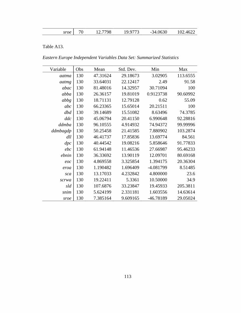
113
sroe 70 12.7798 19.9773 -34.0630 102.4622
Table A13.
Eastern Europe Independent Variables Data Set: Summarized Statistics
Variable Obs Mean Std. Dev. Min Max
aatma 130 47.31624 29.18673 3.02905 113.6555
aatmg 130 33.64031 22.12417 2.49 91.58
abac 130 81.48016 14.32957 30.71094 100
abba 130 26.36157 19.81019 0.9123738 90.60992
abbg 130 18.71131 12.79128 0.62 55.09
abc 130 66.23365 15.65014 20.21511 100
dbd 130 39.14689 15.51082 8.63496 74.3785
ddc 130 45.06794 20.41150 6.990648 92.28816
ddmba 130 96.10555 4.914932 74.94372 99.99996
ddmbagdp 130 50.25458 21.41585 7.880902 103.2874
dll 130 46.41737 17.85836 13.69774 84.561
dpc 130 40.44542 19.08216 5.858646 91.77833
ebc 130 61.94148 11.46536 27.66987 95.46233
ebnin 130 36.33692 13.90119 12.09701 80.69168
eoc 130 4.869558 3.325854 1.394175 20.36304
eroa 130 1.190482 1.696409 -4.081799 8.51485
sca 130 13.17033 4.232842 4.800000 23.6
scrwa 130 19.22411 5.3361 10.50000 34.9
sld 130 107.6876 33.23847 19.45933 205.3811
snim 130 5.624199 2.331181 1.603556 14.63614
sroe 130 7.385164 9.609165 -46.78189 29.05024
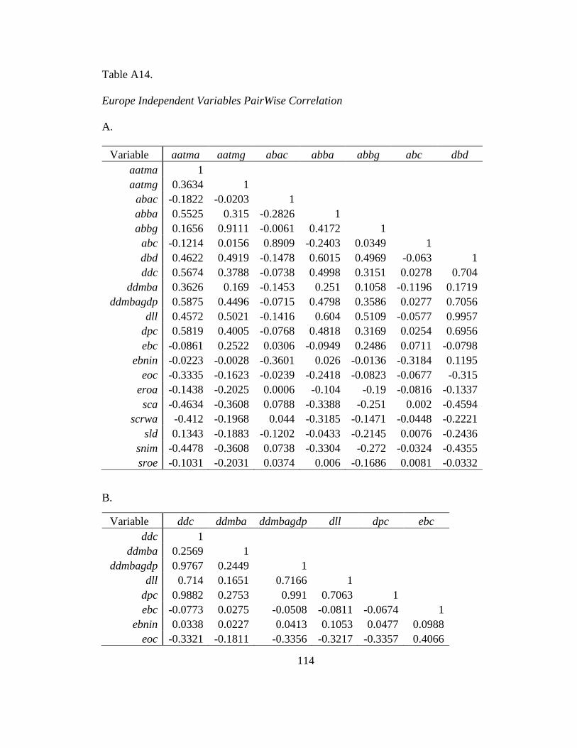
114
Table A14.
Europe Independent Variables PairWise Correlation
A.
Variable aatma aatmg abac abba abbg abc dbd
aatma 1
aatmg 0.3634 1
abac -0.1822 -0.0203 1
abba 0.5525 0.315 -0.2826 1
abbg 0.1656 0.9111 -0.0061 0.4172 1
abc -0.1214 0.0156 0.8909 -0.2403 0.0349 1 dbd 0.4622 0.4919 -0.1478 0.6015 0.4969 -0.063 1
ddc 0.5674 0.3788 -0.0738 0.4998 0.3151 0.0278 0.704
ddmba 0.3626 0.169 -0.1453 0.251 0.1058 -0.1196 0.1719
ddmbagdp 0.5875 0.4496 -0.0715 0.4798 0.3586 0.0277 0.7056
dll 0.4572 0.5021 -0.1416 0.604 0.5109 -0.0577 0.9957
dpc 0.5819 0.4005 -0.0768 0.4818 0.3169 0.0254 0.6956
ebc -0.0861 0.2522 0.0306 -0.0949 0.2486 0.0711 -0.0798
ebnin -0.0223 -0.0028 -0.3601 0.026 -0.0136 -0.3184 0.1195
eoc -0.3335 -0.1623 -0.0239 -0.2418 -0.0823 -0.0677 -0.315
eroa -0.1438 -0.2025 0.0006 -0.104 -0.19 -0.0816 -0.1337
sca -0.4634 -0.3608 0.0788 -0.3388 -0.251 0.002 -0.4594
scrwa -0.412 -0.1968 0.044 -0.3185 -0.1471 -0.0448 -0.2221
sld 0.1343 -0.1883 -0.1202 -0.0433 -0.2145 0.0076 -0.2436
snim -0.4478 -0.3608 0.0738 -0.3304 -0.272 -0.0324 -0.4355
sroe -0.1031 -0.2031 0.0374 0.006 -0.1686 0.0081 -0.0332
B.
Variable ddc ddmba ddmbagdp dll dpc ebc
ddc 1
ddmba 0.2569 1
ddmbagdp 0.9767 0.2449 1
dll 0.714 0.1651 0.7166 1
dpc 0.9882 0.2753 0.991 0.7063 1 ebc -0.0773 0.0275 -0.0508 -0.0811 -0.0674 1
ebnin 0.0338 0.0227 0.0413 0.1053 0.0477 0.0988
eoc -0.3321 -0.1811 -0.3356 -0.3217 -0.3357 0.4066
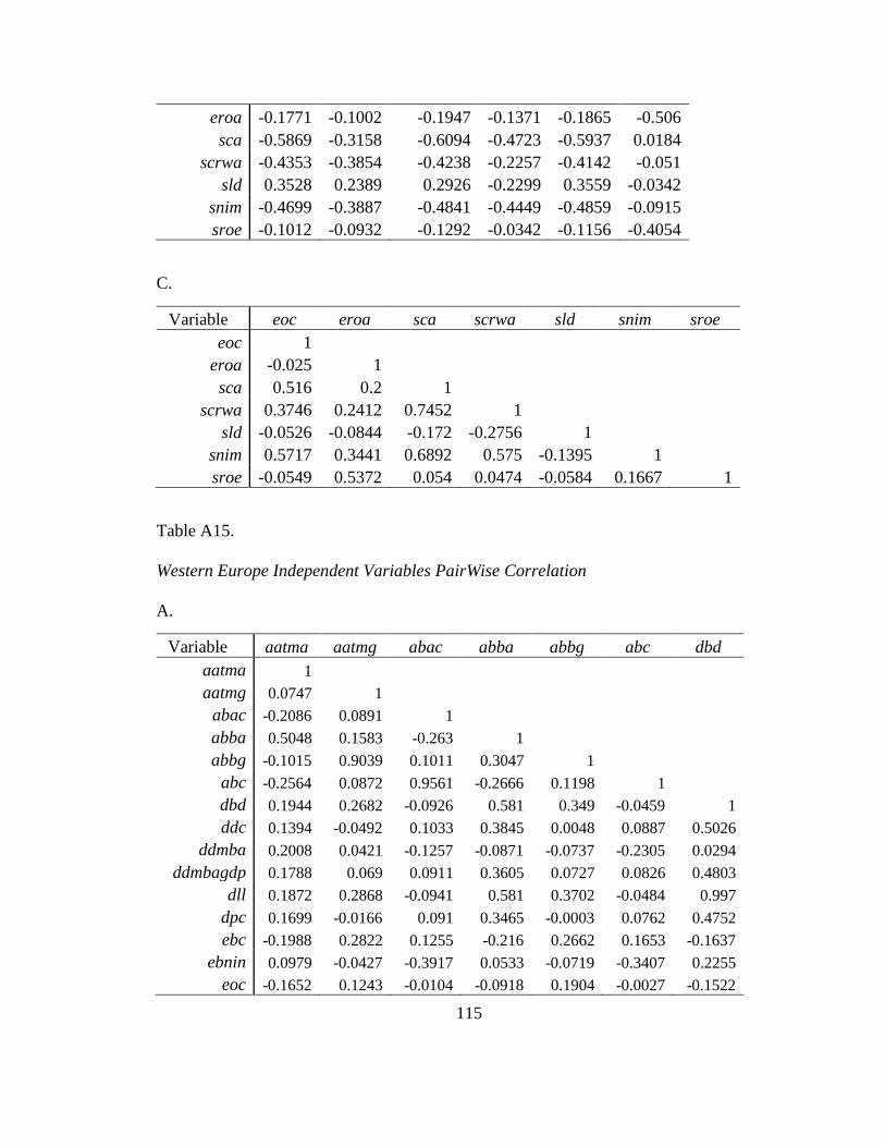
115
eroa -0.1771 -0.1002 -0.1947 -0.1371 -0.1865 -0.506
sca -0.5869 -0.3158 -0.6094 -0.4723 -0.5937 0.0184
scrwa -0.4353 -0.3854 -0.4238 -0.2257 -0.4142 -0.051
sld 0.3528 0.2389 0.2926 -0.2299 0.3559 -0.0342
snim -0.4699 -0.3887 -0.4841 -0.4449 -0.4859 -0.0915
sroe -0.1012 -0.0932 -0.1292 -0.0342 -0.1156 -0.4054
C.
Variable eoc eroa sca scrwa sld snim sroe
eoc 1
eroa -0.025 1
sca 0.516 0.2 1
scrwa 0.3746 0.2412 0.7452 1
sld -0.0526 -0.0844 -0.172 -0.2756 1
snim 0.5717 0.3441 0.6892 0.575 -0.1395 1 sroe -0.0549 0.5372 0.054 0.0474 -0.0584 0.1667 1
Table A15.
Western Europe Independent Variables PairWise Correlation
A.
Variable aatma aatmg abac abba abbg abc dbd
aatma 1
aatmg 0.0747 1
abac -0.2086 0.0891 1
abba 0.5048 0.1583 -0.263 1
abbg -0.1015 0.9039 0.1011 0.3047 1
abc -0.2564 0.0872 0.9561 -0.2666 0.1198 1
dbd 0.1944 0.2682 -0.0926 0.581 0.349 -0.0459 1
ddc 0.1394 -0.0492 0.1033 0.3845 0.0048 0.0887 0.5026
ddmba 0.2008 0.0421 -0.1257 -0.0871 -0.0737 -0.2305 0.0294
ddmbagdp 0.1788 0.069 0.0911 0.3605 0.0727 0.0826 0.4803
dll 0.1872 0.2868 -0.0941 0.581 0.3702 -0.0484 0.997
dpc 0.1699 -0.0166 0.091 0.3465 -0.0003 0.0762 0.4752
ebc -0.1988 0.2822 0.1255 -0.216 0.2662 0.1653 -0.1637
ebnin 0.0979 -0.0427 -0.3917 0.0533 -0.0719 -0.3407 0.2255
eoc -0.1652 0.1243 -0.0104 -0.0918 0.1904 -0.0027 -0.1522
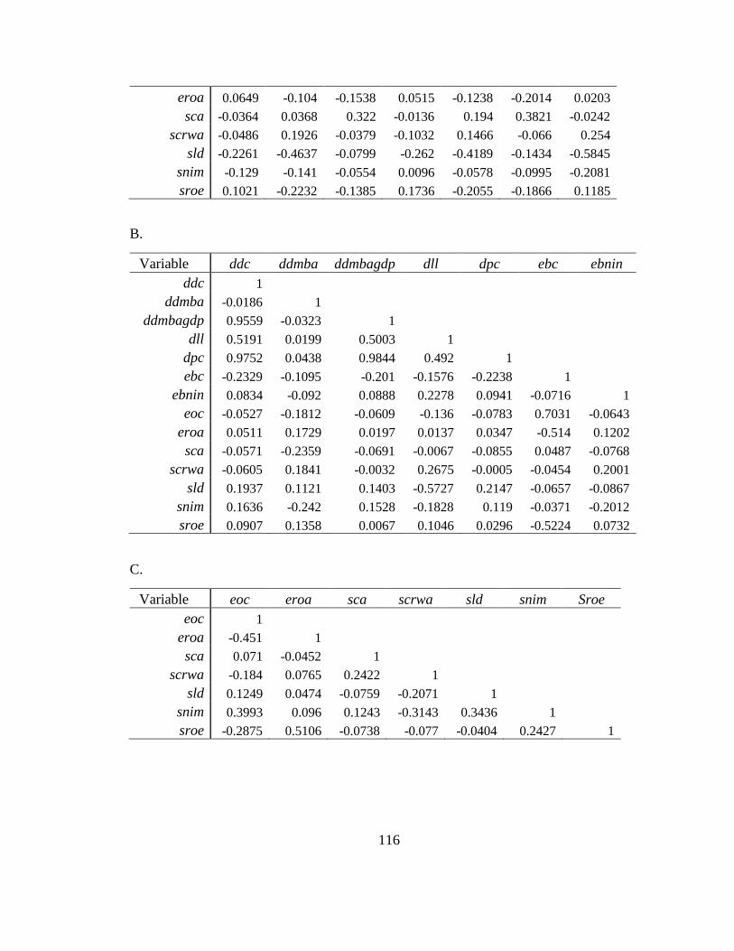
116
eroa 0.0649 -0.104 -0.1538 0.0515 -0.1238 -0.2014 0.0203
sca -0.0364 0.0368 0.322 -0.0136 0.194 0.3821 -0.0242
scrwa -0.0486 0.1926 -0.0379 -0.1032 0.1466 -0.066 0.254
sld -0.2261 -0.4637 -0.0799 -0.262 -0.4189 -0.1434 -0.5845
snim -0.129 -0.141 -0.0554 0.0096 -0.0578 -0.0995 -0.2081
sroe 0.1021 -0.2232 -0.1385 0.1736 -0.2055 -0.1866 0.1185
B.
Variable ddc ddmba ddmbagdp dll dpc ebc ebnin
ddc 1
ddmba -0.0186 1
ddmbagdp 0.9559 -0.0323 1
dll 0.5191 0.0199 0.5003 1
dpc 0.9752 0.0438 0.9844 0.492 1
ebc -0.2329 -0.1095 -0.201 -0.1576 -0.2238 1
ebnin 0.0834 -0.092 0.0888 0.2278 0.0941 -0.0716 1
eoc -0.0527 -0.1812 -0.0609 -0.136 -0.0783 0.7031 -0.0643
eroa 0.0511 0.1729 0.0197 0.0137 0.0347 -0.514 0.1202
sca -0.0571 -0.2359 -0.0691 -0.0067 -0.0855 0.0487 -0.0768
scrwa -0.0605 0.1841 -0.0032 0.2675 -0.0005 -0.0454 0.2001
sld 0.1937 0.1121 0.1403 -0.5727 0.2147 -0.0657 -0.0867
snim 0.1636 -0.242 0.1528 -0.1828 0.119 -0.0371 -0.2012
sroe 0.0907 0.1358 0.0067 0.1046 0.0296 -0.5224 0.0732
C.
Variable eoc eroa sca scrwa sld snim Sroe
eoc 1
eroa -0.451 1
sca 0.071 -0.0452 1
scrwa -0.184 0.0765 0.2422 1
sld 0.1249 0.0474 -0.0759 -0.2071 1
snim 0.3993 0.096 0.1243 -0.3143 0.3436 1
sroe -0.2875 0.5106 -0.0738 -0.077 -0.0404 0.2427 1
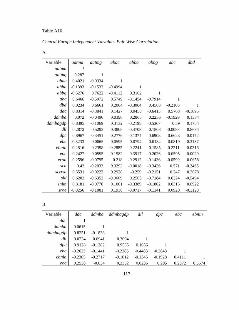
117
Table A16.
Central Europe Independent Variables Pair Wise Correlation
A.
Variable aatma aatmg abac abba abbg abc dbd
aatma 1
aatmg -0.287 1
abac 0.4021 -0.0334 1
abba -0.1393 -0.1533 -0.4994 1
abbg -0.6276 0.7622 -0.4112 0.3162 1
abc 0.6466 -0.5072 0.5749 -0.1454 -0.7914 1
dbd 0.0234 0.6661 0.2064 -0.3064 0.4503 -0.2106 1
ddc 0.8314 -0.3841 0.1427 0.0458 -0.6415 0.5708 -0.1095
ddmba 0.072 -0.0496 0.0398 0.2865 0.2256 -0.1929 0.1334
ddmbagdp 0.8395 -0.1069 0.3132 -0.2198 -0.5367 0.59 0.1784
dll 0.2872 0.5293 0.3805 -0.4708 0.1808 -0.0088 0.8634
dpc 0.8967 -0.3451 0.2776 -0.1374 -0.6908 0.6623 -0.0172
ebc -0.3233 0.0065 0.0595 0.0794 0.0184 0.0819 -0.3187
ebnin -0.2816 0.2398 -0.2885 -0.2241 0.1585 -0.2211 -0.0316
eoc 0.2427 0.0595 0.1582 -0.3917 -0.2026 0.0595 -0.0029
eroa 0.2596 -0.0795 0.218 -0.2912 -0.1436 -0.0599 0.0658
sca 0.43 -0.2033 0.3292 -0.0018 -0.3426 0.571 -0.2465
scrwa 0.5531 -0.0223 0.2928 -0.259 -0.2151 0.347 0.3678
sld 0.6202 -0.6352 -0.0609 0.2505 -0.7184 0.6324 -0.5494
snim 0.3181 -0.0778 0.1061 -0.3389 -0.1802 0.0315 0.0922
sroe -0.0256 -0.1881 0.1938 -0.0717 -0.1141 0.0928 -0.1128
B.
Variable ddc ddmba ddmbagdp dll dpc ebc ebnin
ddc 1
ddmba -0.0615 1
ddmbagdp 0.8251 -0.1838 1
dll 0.0724 0.0941 0.3094 1
dpc 0.9128 -0.1282 0.9565 0.1656 1
ebc -0.2625 -0.1441 -0.2285 -0.4483 -0.2843 1
ebnin -0.2365 -0.2717 -0.1012 -0.1346 -0.1928 0.4111 1
eoc 0.2538 -0.034 0.3352 0.0236 0.285 0.2372 0.5674
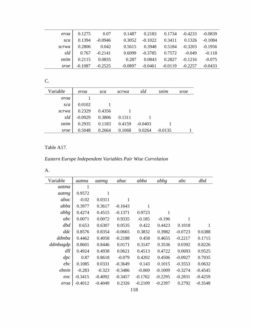
118
eroa 0.1275 0.07 0.1487 0.2183 0.1734 -0.4233 -0.0839
sca 0.1394 -0.0946 0.3052 -0.1022 0.3411 0.1326 -0.1084
scrwa 0.2806 0.042 0.5615 0.3948 0.5184 -0.3203 -0.1956
sld 0.767 -0.2141 0.6099 -0.3785 0.7572 -0.049 -0.118
snim 0.2115 0.0835 0.287 0.0843 0.2827 -0.1216 -0.075
sroe -0.1087 -0.2525 -0.0897 -0.0461 -0.0119 -0.2257 -0.0433
C.
Variable eroa sca scrwa sld snim sroe
eroa 1
sca 0.0102 1
scrwa 0.2329 0.4356 1
sld -0.0929 0.3806 0.1311 1
snim 0.2935 0.1183 0.4159 -0.0403 1
sroe 0.5048 0.2664 0.1068 0.0264 -0.0135 1
Table A17.
Eastern Europe Independent Variables Pair Wise Correlation
A.
Variable aatma aatmg abac abba abbg abc dbd
aatma 1
aatmg 0.9572 1
abac -0.02 0.0311 1
abba 0.3977 0.3617 -0.1643 1
abbg 0.4274 0.4515 -0.1371 0.9723 1
abc 0.0071 0.0072 0.9335 -0.185 -0.196 1
dbd 0.653 0.6307 0.0535 0.422 0.4423 0.1018 1
ddc 0.8576 0.8354 -0.0665 0.3832 0.3982 -0.0723 0.6388
ddmba 0.4462 0.4058 -0.2188 0.458 0.4655 -0.2217 0.1715
ddmbagdp 0.8601 0.8446 0.0171 0.3147 0.3536 0.0392 0.8226
dll 0.4924 0.4938 0.0621 0.4513 0.4722 0.0693 0.9525
dpc 0.87 0.8618 -0.079 0.4202 0.4506 -0.0927 0.7035
ebc 0.1085 0.0331 -0.3649 0.143 0.1015 -0.3553 0.0632
ebnin -0.283 -0.323 -0.3486 -0.069 -0.1009 -0.3274 -0.4545
eoc -0.3415 -0.4092 -0.3457 -0.1762 -0.2295 -0.2831 -0.4259
eroa -0.4012 -0.4049 0.2326 -0.2109 -0.2397 0.2792 -0.3548
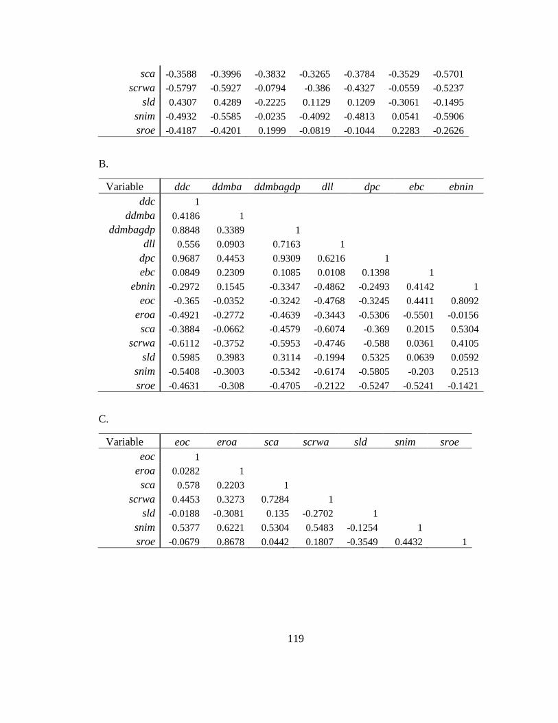
119
sca -0.3588 -0.3996 -0.3832 -0.3265 -0.3784 -0.3529 -0.5701
scrwa -0.5797 -0.5927 -0.0794 -0.386 -0.4327 -0.0559 -0.5237
sld 0.4307 0.4289 -0.2225 0.1129 0.1209 -0.3061 -0.1495
snim -0.4932 -0.5585 -0.0235 -0.4092 -0.4813 0.0541 -0.5906
sroe -0.4187 -0.4201 0.1999 -0.0819 -0.1044 0.2283 -0.2626
B.
Variable ddc ddmba ddmbagdp dll dpc ebc ebnin
ddc 1
ddmba 0.4186 1
ddmbagdp 0.8848 0.3389 1
dll 0.556 0.0903 0.7163 1
dpc 0.9687 0.4453 0.9309 0.6216 1
ebc 0.0849 0.2309 0.1085 0.0108 0.1398 1
ebnin -0.2972 0.1545 -0.3347 -0.4862 -0.2493 0.4142 1
eoc -0.365 -0.0352 -0.3242 -0.4768 -0.3245 0.4411 0.8092
eroa -0.4921 -0.2772 -0.4639 -0.3443 -0.5306 -0.5501 -0.0156
sca -0.3884 -0.0662 -0.4579 -0.6074 -0.369 0.2015 0.5304
scrwa -0.6112 -0.3752 -0.5953 -0.4746 -0.588 0.0361 0.4105
sld 0.5985 0.3983 0.3114 -0.1994 0.5325 0.0639 0.0592
snim -0.5408 -0.3003 -0.5342 -0.6174 -0.5805 -0.203 0.2513
sroe -0.4631 -0.308 -0.4705 -0.2122 -0.5247 -0.5241 -0.1421
C.
Variable eoc eroa sca scrwa sld snim sroe
eoc 1
eroa 0.0282 1
sca 0.578 0.2203 1
scrwa 0.4453 0.3273 0.7284 1
sld -0.0188 -0.3081 0.135 -0.2702 1
snim 0.5377 0.6221 0.5304 0.5483 -0.1254 1
sroe -0.0679 0.8678 0.0442 0.1807 -0.3549 0.4432 1
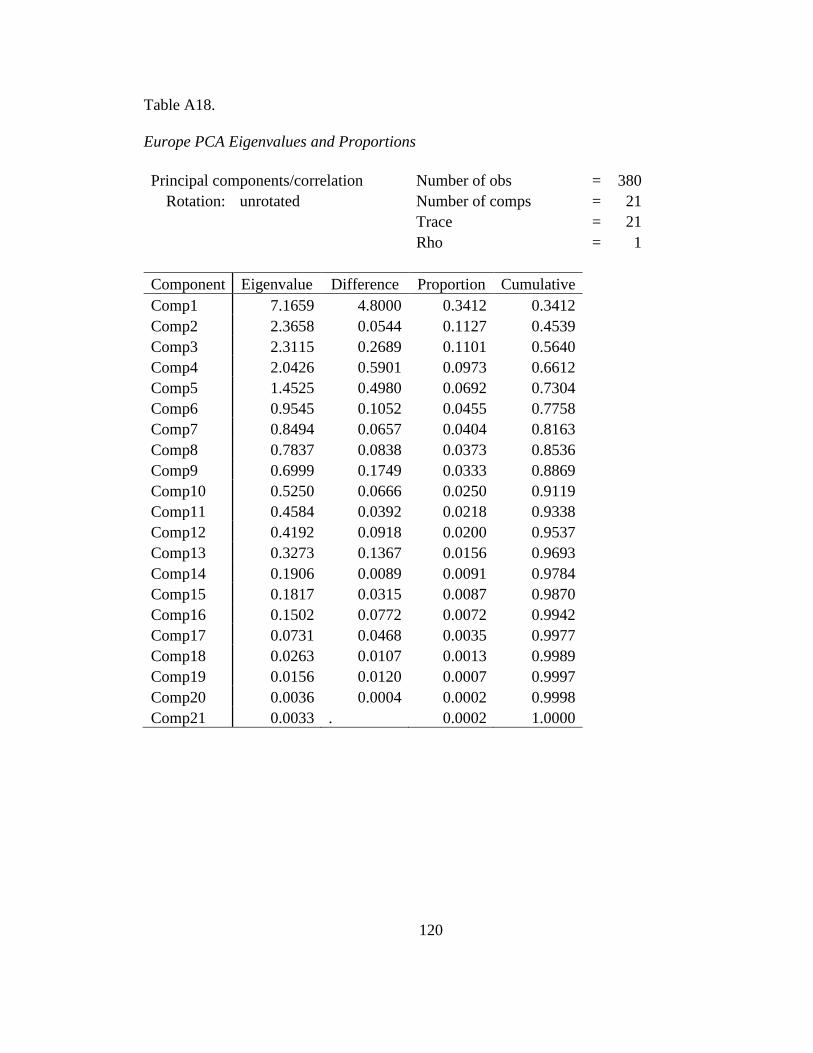
120
Table A18.
Europe PCA Eigenvalues and Proportions
Principal components/correlation Number of obs = 380
Rotation: unrotated Number of comps = 21
Trace = 21
Rho = 1
Component Eigenvalue Difference Proportion Cumulative
Comp1 7.1659 4.8000 0.3412 0.3412
Comp2 2.3658 0.0544 0.1127 0.4539
Comp3 2.3115 0.2689 0.1101 0.5640
Comp4 2.0426 0.5901 0.0973 0.6612
Comp5 1.4525 0.4980 0.0692 0.7304
Comp6 0.9545 0.1052 0.0455 0.7758
Comp7 0.8494 0.0657 0.0404 0.8163
Comp8 0.7837 0.0838 0.0373 0.8536
Comp9 0.6999 0.1749 0.0333 0.8869
Comp10 0.5250 0.0666 0.0250 0.9119
Comp11 0.4584 0.0392 0.0218 0.9338
Comp12 0.4192 0.0918 0.0200 0.9537
Comp13 0.3273 0.1367 0.0156 0.9693
Comp14 0.1906 0.0089 0.0091 0.9784
Comp15 0.1817 0.0315 0.0087 0.9870
Comp16 0.1502 0.0772 0.0072 0.9942
Comp17 0.0731 0.0468 0.0035 0.9977
Comp18 0.0263 0.0107 0.0013 0.9989
Comp19 0.0156 0.0120 0.0007 0.9997
Comp20 0.0036 0.0004 0.0002 0.9998
Comp21 0.0033 . 0.0002 1.0000
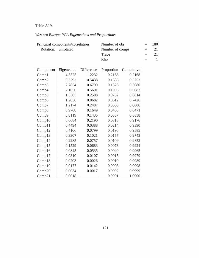
121
Table A19.
Western Europe PCA Eigenvalues and Proportions
Principal components/correlation Number of obs = 180
Rotation: unrotated Number of comps = 21
Trace = 21
Rho = 1
Component Eigenvalue Difference Proportion Cumulative
Comp1 4.5525 1.2232 0.2168 0.2168
Comp2 3.3293 0.5438 0.1585 0.3753
Comp3 2.7854 0.6799 0.1326 0.5080
Comp4 2.1056 0.5691 0.1003 0.6082
Comp5 1.5365 0.2508 0.0732 0.6814
Comp6 1.2856 0.0682 0.0612 0.7426
Comp7 1.2174 0.2407 0.0580 0.8006
Comp8 0.9768 0.1649 0.0465 0.8471
Comp9 0.8119 0.1435 0.0387 0.8858
Comp10 0.6684 0.2190 0.0318 0.9176
Comp11 0.4494 0.0388 0.0214 0.9390
Comp12 0.4106 0.0799 0.0196 0.9585
Comp13 0.3307 0.1021 0.0157 0.9743
Comp14 0.2285 0.0757 0.0109 0.9852
Comp15 0.1529 0.0683 0.0073 0.9924
Comp16 0.0845 0.0535 0.0040 0.9965
Comp17 0.0310 0.0107 0.0015 0.9979
Comp18 0.0203 0.0026 0.0010 0.9989
Comp19 0.0177 0.0142 0.0008 0.9998
Comp20 0.0034 0.0017 0.0002 0.9999
Comp21 0.0018 . 0.0001 1.0000
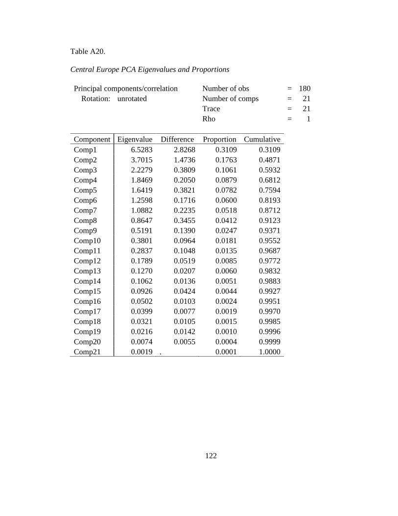
122
Table A20.
Central Europe PCA Eigenvalues and Proportions
Principal components/correlation Number of obs = 180
Rotation: unrotated Number of comps = 21
Trace = 21
Rho = 1
Component Eigenvalue Difference Proportion Cumulative
Comp1 6.5283 2.8268 0.3109 0.3109
Comp2 3.7015 1.4736 0.1763 0.4871
Comp3 2.2279 0.3809 0.1061 0.5932
Comp4 1.8469 0.2050 0.0879 0.6812
Comp5 1.6419 0.3821 0.0782 0.7594
Comp6 1.2598 0.1716 0.0600 0.8193
Comp7 1.0882 0.2235 0.0518 0.8712
Comp8 0.8647 0.3455 0.0412 0.9123
Comp9 0.5191 0.1390 0.0247 0.9371
Comp10 0.3801 0.0964 0.0181 0.9552
Comp11 0.2837 0.1048 0.0135 0.9687
Comp12 0.1789 0.0519 0.0085 0.9772
Comp13 0.1270 0.0207 0.0060 0.9832
Comp14 0.1062 0.0136 0.0051 0.9883
Comp15 0.0926 0.0424 0.0044 0.9927
Comp16 0.0502 0.0103 0.0024 0.9951
Comp17 0.0399 0.0077 0.0019 0.9970
Comp18 0.0321 0.0105 0.0015 0.9985
Comp19 0.0216 0.0142 0.0010 0.9996
Comp20 0.0074 0.0055 0.0004 0.9999
Comp21 0.0019 . 0.0001 1.0000
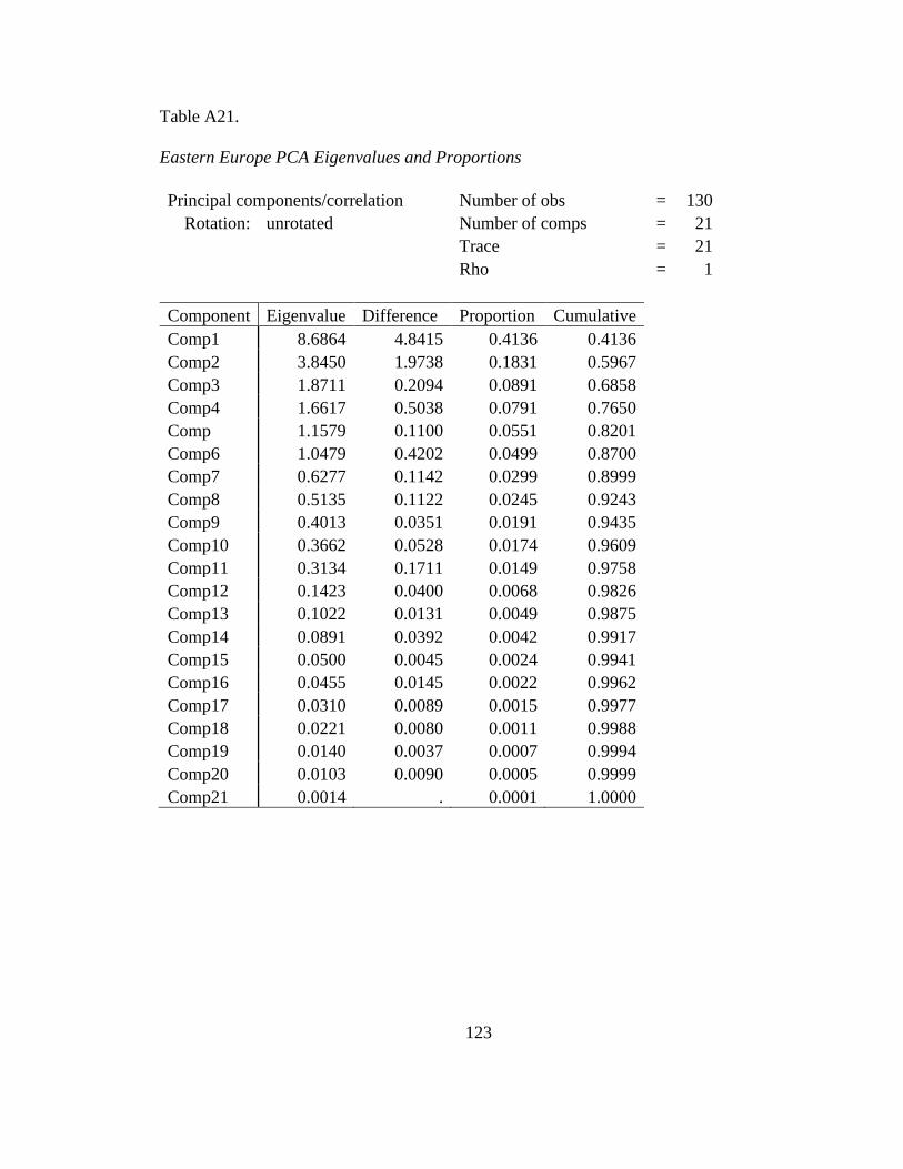
123
Table A21.
Eastern Europe PCA Eigenvalues and Proportions
Principal components/correlation Number of obs = 130
Rotation: unrotated Number of comps = 21
Trace = 21
Rho = 1
Component Eigenvalue Difference Proportion Cumulative
Comp1 8.6864 4.8415 0.4136 0.4136
Comp2 3.8450 1.9738 0.1831 0.5967
Comp3 1.8711 0.2094 0.0891 0.6858
Comp4 1.6617 0.5038 0.0791 0.7650
Comp 1.1579 0.1100 0.0551 0.8201
Comp6 1.0479 0.4202 0.0499 0.8700
Comp7 0.6277 0.1142 0.0299 0.8999
Comp8 0.5135 0.1122 0.0245 0.9243
Comp9 0.4013 0.0351 0.0191 0.9435
Comp10 0.3662 0.0528 0.0174 0.9609
Comp11 0.3134 0.1711 0.0149 0.9758
Comp12 0.1423 0.0400 0.0068 0.9826
Comp13 0.1022 0.0131 0.0049 0.9875
Comp14 0.0891 0.0392 0.0042 0.9917
Comp15 0.0500 0.0045 0.0024 0.9941
Comp16 0.0455 0.0145 0.0022 0.9962
Comp17 0.0310 0.0089 0.0015 0.9977
Comp18 0.0221 0.0080 0.0011 0.9988
Comp19 0.0140 0.0037 0.0007 0.9994
Comp20 0.0103 0.0090 0.0005 0.9999
Comp21 0.0014 . 0.0001 1.0000
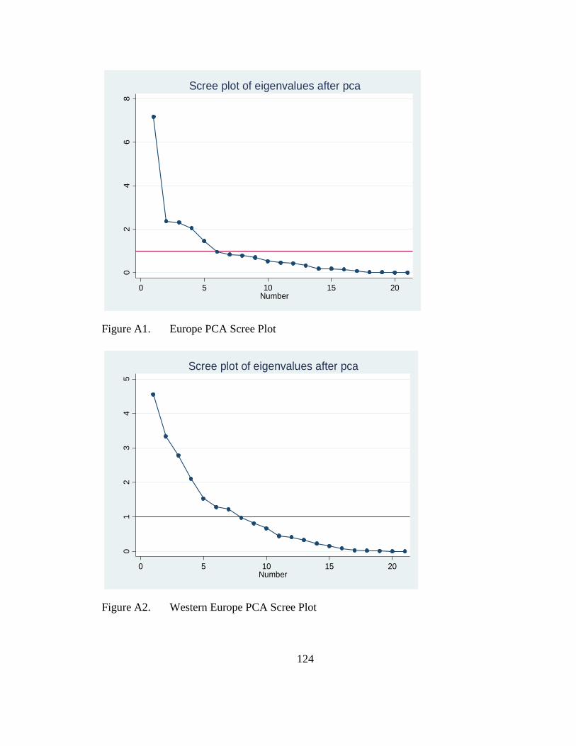
124
Figure A1. Europe PCA Scree Plot
Figure A2. Western Europe PCA Scree Plot
02
46
8
Eig
enva
lues
0 5 10 15 20Number
Scree plot of eigenvalues after pca
01
23
45
Eig
enva
lues
0 5 10 15 20Number
Scree plot of eigenvalues after pca
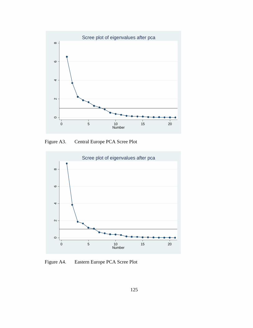
125
Figure A3. Central Europe PCA Scree Plot
Figure A4. Eastern Europe PCA Scree Plot
02
46
8
Eig
enva
lues
0 5 10 15 20Number
Scree plot of eigenvalues after pca
02
46
8
Eig
enva
lues
0 5 10 15 20Number
Scree plot of eigenvalues after pca
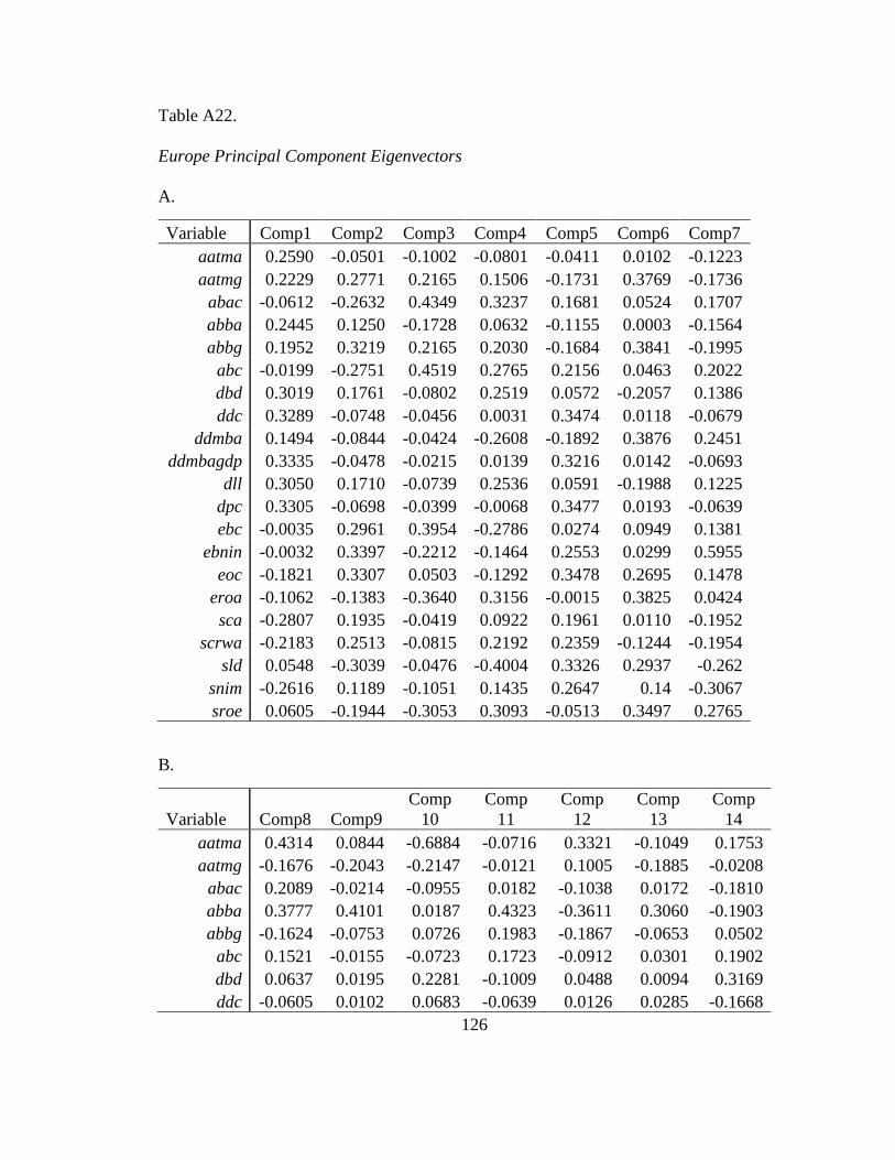
126
Table A22.
Europe Principal Component Eigenvectors
A.
Variable Comp1 Comp2 Comp3 Comp4 Comp5 Comp6 Comp7
aatma 0.2590 -0.0501 -0.1002 -0.0801 -0.0411 0.0102 -0.1223
aatmg 0.2229 0.2771 0.2165 0.1506 -0.1731 0.3769 -0.1736
abac -0.0612 -0.2632 0.4349 0.3237 0.1681 0.0524 0.1707
abba 0.2445 0.1250 -0.1728 0.0632 -0.1155 0.0003 -0.1564
abbg 0.1952 0.3219 0.2165 0.2030 -0.1684 0.3841 -0.1995
abc -0.0199 -0.2751 0.4519 0.2765 0.2156 0.0463 0.2022
dbd 0.3019 0.1761 -0.0802 0.2519 0.0572 -0.2057 0.1386
ddc 0.3289 -0.0748 -0.0456 0.0031 0.3474 0.0118 -0.0679
ddmba 0.1494 -0.0844 -0.0424 -0.2608 -0.1892 0.3876 0.2451
ddmbagdp 0.3335 -0.0478 -0.0215 0.0139 0.3216 0.0142 -0.0693
dll 0.3050 0.1710 -0.0739 0.2536 0.0591 -0.1988 0.1225
dpc 0.3305 -0.0698 -0.0399 -0.0068 0.3477 0.0193 -0.0639
ebc -0.0035 0.2961 0.3954 -0.2786 0.0274 0.0949 0.1381
ebnin -0.0032 0.3397 -0.2212 -0.1464 0.2553 0.0299 0.5955
eoc -0.1821 0.3307 0.0503 -0.1292 0.3478 0.2695 0.1478
eroa -0.1062 -0.1383 -0.3640 0.3156 -0.0015 0.3825 0.0424
sca -0.2807 0.1935 -0.0419 0.0922 0.1961 0.0110 -0.1952
scrwa -0.2183 0.2513 -0.0815 0.2192 0.2359 -0.1244 -0.1954
sld 0.0548 -0.3039 -0.0476 -0.4004 0.3326 0.2937 -0.262
snim -0.2616 0.1189 -0.1051 0.1435 0.2647 0.14 -0.3067
sroe 0.0605 -0.1944 -0.3053 0.3093 -0.0513 0.3497 0.2765
B.
Variable Comp8 Comp9
Comp
10
Comp
11
Comp
12
Comp
13
Comp
14
aatma 0.4314 0.0844 -0.6884 -0.0716 0.3321 -0.1049 0.1753
aatmg -0.1676 -0.2043 -0.2147 -0.0121 0.1005 -0.1885 -0.0208
abac 0.2089 -0.0214 -0.0955 0.0182 -0.1038 0.0172 -0.1810
abba 0.3777 0.4101 0.0187 0.4323 -0.3611 0.3060 -0.1903
abbg -0.1624 -0.0753 0.0726 0.1983 -0.1867 -0.0653 0.0502
abc 0.1521 -0.0155 -0.0723 0.1723 -0.0912 0.0301 0.1902
dbd 0.0637 0.0195 0.2281 -0.1009 0.0488 0.0094 0.3169
ddc -0.0605 0.0102 0.0683 -0.0639 0.0126 0.0285 -0.1668
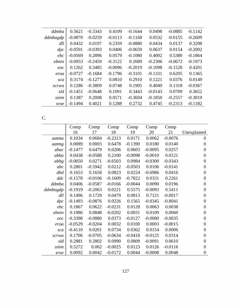
127
ddmba 0.5621 -0.3343 0.4109 -0.1644 0.0498 -0.0885 -0.1142
ddmbagdp -0.0870 -0.0259 -0.0113 -0.1168 0.0532 -0.0155 -0.2609
dll 0.0432 0.0197 0.2359 -0.0880 0.0434 0.0137 0.3208
dpc -0.0591 -0.0393 0.0406 -0.0659 0.0637 0.0154 -0.2002
ebc -0.0569 0.2896 0.0579 -0.1080 0.4002 0.5380 -0.1864
ebnin -0.0953 -0.2459 -0.3122 0.2689 -0.2306 -0.0672 -0.1973
eoc 0.1262 0.3485 -0.0096 -0.2019 -0.1098 -0.1528 0.4201
eroa -0.0727 -0.1684 -0.1796 -0.3101 -0.1331 0.6205 0.1365
sca 0.3174 -0.1277 0.0810 0.2910 0.1221 0.0376 0.0149
scrwa 0.1286 -0.3809 0.0748 0.1905 0.4049 0.1318 -0.0367
sld -0.1451 -0.0648 0.1091 0.3443 -0.0143 0.0709 0.3652
snim 0.1387 0.2008 0.0571 -0.3694 -0.1850 -0.2557 -0.3019
sroe -0.1494 0.4021 0.1288 0.2732 0.4745 -0.2313 -0.1182
C.
Comp
16
Comp
17
Comp
18
Comp
19
Comp
20
Comp
21 Unexplained
aatma 0.1034 0.0684 -0.2313 0.0171 0.0062 -0.0076 0
aatmg 0.0089 0.0003 0.6478 -0.1390 0.0180 0.0140 0
abac -0.1477 0.6479 0.0206 0.0603 -0.0095 0.0257 0
abba 0.0438 -0.0588 0.2100 -0.0098 -0.0010 0.0121 0
abbg -0.0050 0.0271 -0.6503 0.0984 -0.0300 -0.0343 0
abc 0.2801 -0.5942 0.0212 -0.0503 0.0106 -0.0141 0
dbd 0.1653 0.1658 0.0823 0.0224 -0.6986 0.0416 0
ddc -0.1578 -0.0106 -0.1609 -0.7822 0.0331 0.2261 0
ddmba 0.0406 -0.0587 -0.0166 -0.0044 0.0090 0.0196 0
ddmbagdp -0.1919 -0.2063 0.0221 0.5575 -0.0093 0.5411 0
dll 0.1496 0.1729 0.0479 0.0813 0.7121 -0.0017 0
dpc -0.1493 -0.0876 0.0226 0.1565 -0.0345 -0.8041 0
ebc 0.1867 0.0622 -0.0231 0.0128 0.0063 0.0038 0
ebnin 0.1986 0.0848 -0.0202 0.0031 0.0109 0.0060 0
eoc -0.3398 -0.0880 0.0373 -0.0127 -0.0080 -0.0035 0
eroa -0.0529 -0.0204 0.0032 0.0100 0.0003 -0.0015 0
sca -0.4110 0.0201 0.0734 0.0362 0.0154 0.0006 0
scrwa 0.1706 -0.0705 -0.0634 -0.0418 -0.0125 0.0314 0
sld 0.2881 0.2802 0.0990 0.0809 -0.0091 0.0610 0
snim 0.5272 0.062 -0.0025 0.0123 0.0126 -0.0116 0
sroe 0.0092 0.0042 -0.0172 0.0044 -0.0008 0.0048 0
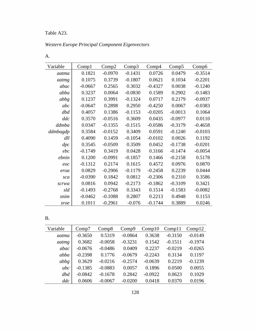
128
Table A23.
Western Europe Principal Component Eigenvectors
A.
Variable Comp1 Comp2 Comp3 Comp4 Comp5 Comp6
aatma 0.1821 -0.0970 -0.1431 0.0726 0.0479 -0.3514
aatmg 0.1075 0.3739 -0.1807 0.0621 0.1034 -0.2201
abac -0.0667 0.2565 0.3032 -0.4327 0.0038 -0.1240
abba 0.3237 0.0064 -0.0830 0.1589 0.2902 -0.1483
abbg 0.1237 0.3991 -0.1324 0.0717 0.2179 -0.0937
abc -0.0647 0.2898 0.2950 -0.4250 0.0067 -0.0383
dbd 0.4057 0.1386 -0.1153 -0.0205 -0.0013 0.1064
ddc 0.3570 -0.0516 0.3609 0.0435 -0.0977 0.0110
ddmba 0.0347 -0.1355 -0.1515 -0.0586 -0.3179 -0.4658
ddmbagdp 0.3584 -0.0152 0.3409 0.0591 -0.1240 -0.0103
dll 0.4090 0.1459 -0.1054 -0.0102 0.0026 0.1192
dpc 0.3545 -0.0509 0.3509 0.0452 -0.1738 -0.0201
ebc -0.1749 0.3419 0.0428 0.3166 -0.1474 -0.0054
ebnin 0.1200 -0.0991 -0.1857 0.1466 -0.2158 0.5178
eoc -0.1312 0.2174 0.1615 0.4572 0.0976 0.0870
eroa 0.0829 -0.2906 -0.1179 -0.2458 0.2239 0.0444
sca -0.0390 0.1842 0.0812 -0.2306 0.2310 0.3586
scrwa 0.0816 0.0942 -0.2173 -0.1862 -0.3109 0.3421
sld -0.1493 -0.2768 0.3343 0.1514 -0.1583 -0.0082
snim -0.0462 -0.1088 0.2807 0.2213 0.4948 0.1153
sroe 0.1011 -0.2961 -0.076 -0.1744 0.3889 0.0246
B.
Variable Comp7 Comp8 Comp9 Comp10 Comp11 Comp12
aatma -0.3650 0.5319 -0.0864 0.3638 -0.3150 -0.0149
aatmg 0.3682 -0.0058 -0.3231 0.1542 -0.1511 -0.1974
abac -0.0676 -0.0486 0.0409 0.2237 -0.0219 -0.0265
abba -0.2398 0.1776 -0.0679 -0.2243 0.3134 0.1197
abbg 0.3629 -0.0216 -0.2574 -0.0639 0.2219 -0.1239
abc -0.1385 -0.0883 0.0057 0.1896 0.0500 0.0055
dbd -0.0842 -0.1678 0.2842 -0.0922 0.0623 0.1029
ddc 0.0606 -0.0067 -0.0200 0.0418 0.0370 0.0196
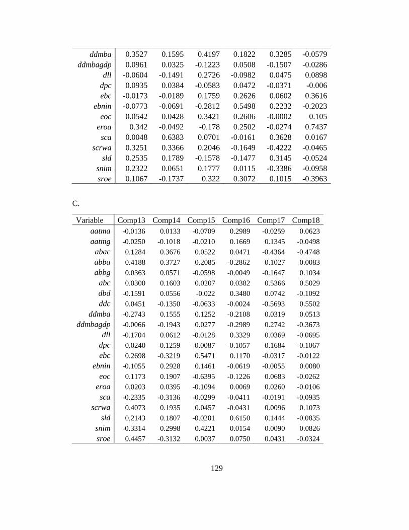
129
ddmba 0.3527 0.1595 0.4197 0.1822 0.3285 -0.0579
ddmbagdp 0.0961 0.0325 -0.1223 0.0508 -0.1507 -0.0286
dll -0.0604 -0.1491 0.2726 -0.0982 0.0475 0.0898
dpc 0.0935 0.0384 -0.0583 0.0472 -0.0371 -0.006
ebc -0.0173 -0.0189 0.1759 0.2626 0.0602 0.3616
ebnin -0.0773 -0.0691 -0.2812 0.5498 0.2232 -0.2023
eoc 0.0542 0.0428 0.3421 0.2606 -0.0002 0.105
eroa 0.342 -0.0492 -0.178 0.2502 -0.0274 0.7437
sca 0.0048 0.6383 0.0701 -0.0161 0.3628 0.0167
scrwa 0.3251 0.3366 0.2046 -0.1649 -0.4222 -0.0465
sld 0.2535 0.1789 -0.1578 -0.1477 0.3145 -0.0524
snim 0.2322 0.0651 0.1777 0.0115 -0.3386 -0.0958
sroe 0.1067 -0.1737 0.322 0.3072 0.1015 -0.3963
C.
Variable Comp13 Comp14 Comp15 Comp16 Comp17 Comp18
aatma -0.0136 0.0133 -0.0709 0.2989 -0.0259 0.0623
aatmg -0.0250 -0.1018 -0.0210 0.1669 0.1345 -0.0498
abac 0.1284 0.3676 0.0522 0.0471 -0.4364 -0.4748
abba 0.4188 0.3727 0.2085 -0.2862 0.1027 0.0083
abbg 0.0363 0.0571 -0.0598 -0.0049 -0.1647 0.1034
abc 0.0300 0.1603 0.0207 0.0382 0.5366 0.5029
dbd -0.1591 0.0556 -0.022 0.3480 0.0742 -0.1092
ddc 0.0451 -0.1350 -0.0633 -0.0024 -0.5693 0.5502
ddmba -0.2743 0.1555 0.1252 -0.2108 0.0319 0.0513
ddmbagdp -0.0066 -0.1943 0.0277 -0.2989 0.2742 -0.3673
dll -0.1704 0.0612 -0.0128 0.3329 0.0369 -0.0695
dpc 0.0240 -0.1259 -0.0087 -0.1057 0.1684 -0.1067
ebc 0.2698 -0.3219 0.5471 0.1170 -0.0317 -0.0122
ebnin -0.1055 0.2928 0.1461 -0.0619 -0.0055 0.0080
eoc 0.1173 0.1907 -0.6395 -0.1226 0.0683 -0.0262
eroa 0.0203 0.0395 -0.1094 0.0069 0.0260 -0.0106
sca -0.2335 -0.3136 -0.0299 -0.0411 -0.0191 -0.0935
scrwa 0.4073 0.1935 0.0457 -0.0431 0.0096 0.1073
sld 0.2143 0.1807 -0.0201 0.6150 0.1444 -0.0835
snim -0.3314 0.2998 0.4221 0.0154 0.0090 0.0826
sroe 0.4457 -0.3132 0.0037 0.0750 0.0431 -0.0324
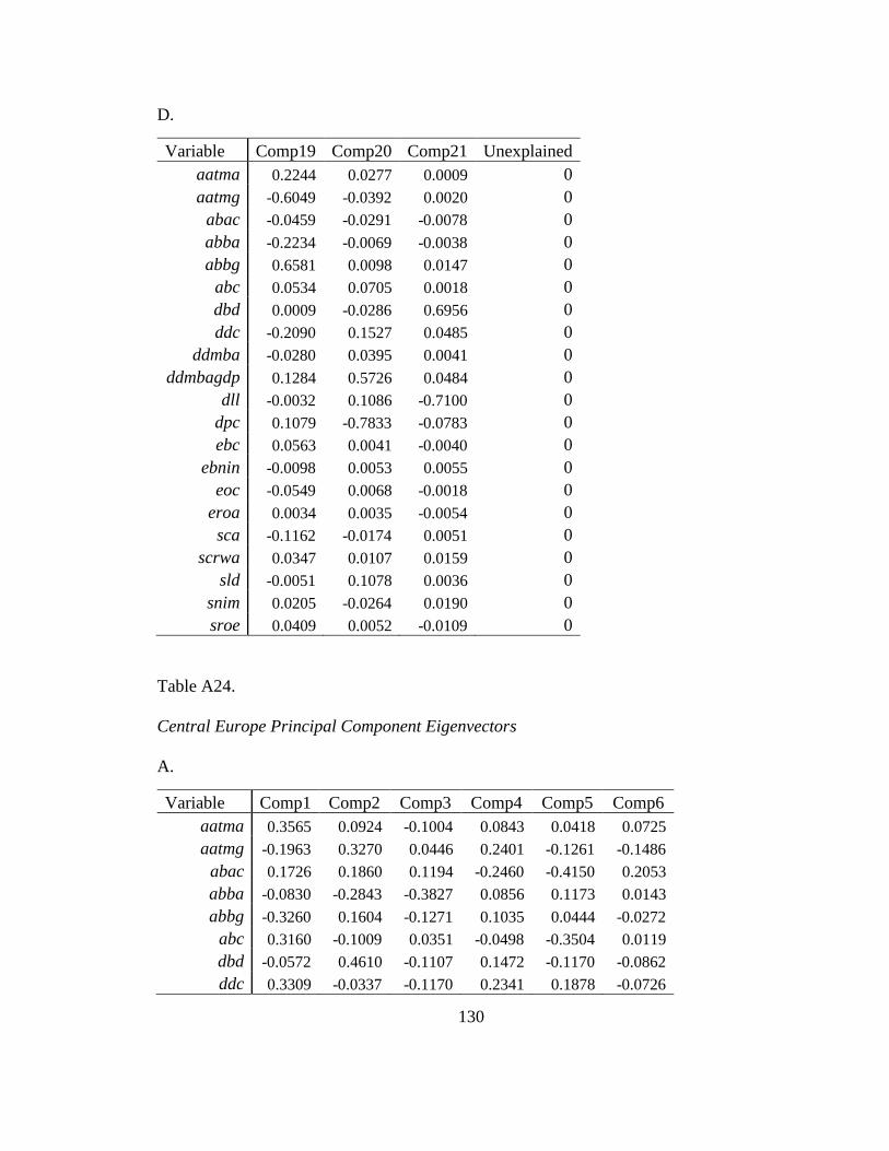
130
D.
Variable Comp19 Comp20 Comp21 Unexplained
aatma 0.2244 0.0277 0.0009 0
aatmg -0.6049 -0.0392 0.0020 0
abac -0.0459 -0.0291 -0.0078 0
abba -0.2234 -0.0069 -0.0038 0
abbg 0.6581 0.0098 0.0147 0
abc 0.0534 0.0705 0.0018 0
dbd 0.0009 -0.0286 0.6956 0
ddc -0.2090 0.1527 0.0485 0
ddmba -0.0280 0.0395 0.0041 0
ddmbagdp 0.1284 0.5726 0.0484 0
dll -0.0032 0.1086 -0.7100 0
dpc 0.1079 -0.7833 -0.0783 0
ebc 0.0563 0.0041 -0.0040 0
ebnin -0.0098 0.0053 0.0055 0
eoc -0.0549 0.0068 -0.0018 0
eroa 0.0034 0.0035 -0.0054 0
sca -0.1162 -0.0174 0.0051 0
scrwa 0.0347 0.0107 0.0159 0
sld -0.0051 0.1078 0.0036 0
snim 0.0205 -0.0264 0.0190 0
sroe 0.0409 0.0052 -0.0109 0
Table A24.
Central Europe Principal Component Eigenvectors
A.
Variable Comp1 Comp2 Comp3 Comp4 Comp5 Comp6
aatma 0.3565 0.0924 -0.1004 0.0843 0.0418 0.0725
aatmg -0.1963 0.3270 0.0446 0.2401 -0.1261 -0.1486
abac 0.1726 0.1860 0.1194 -0.2460 -0.4150 0.2053
abba -0.0830 -0.2843 -0.3827 0.0856 0.1173 0.0143
abbg -0.3260 0.1604 -0.1271 0.1035 0.0444 -0.0272
abc 0.3160 -0.1009 0.0351 -0.0498 -0.3504 0.0119
dbd -0.0572 0.4610 -0.1107 0.1472 -0.1170 -0.0862
ddc 0.3309 -0.0337 -0.1170 0.2341 0.1878 -0.0726
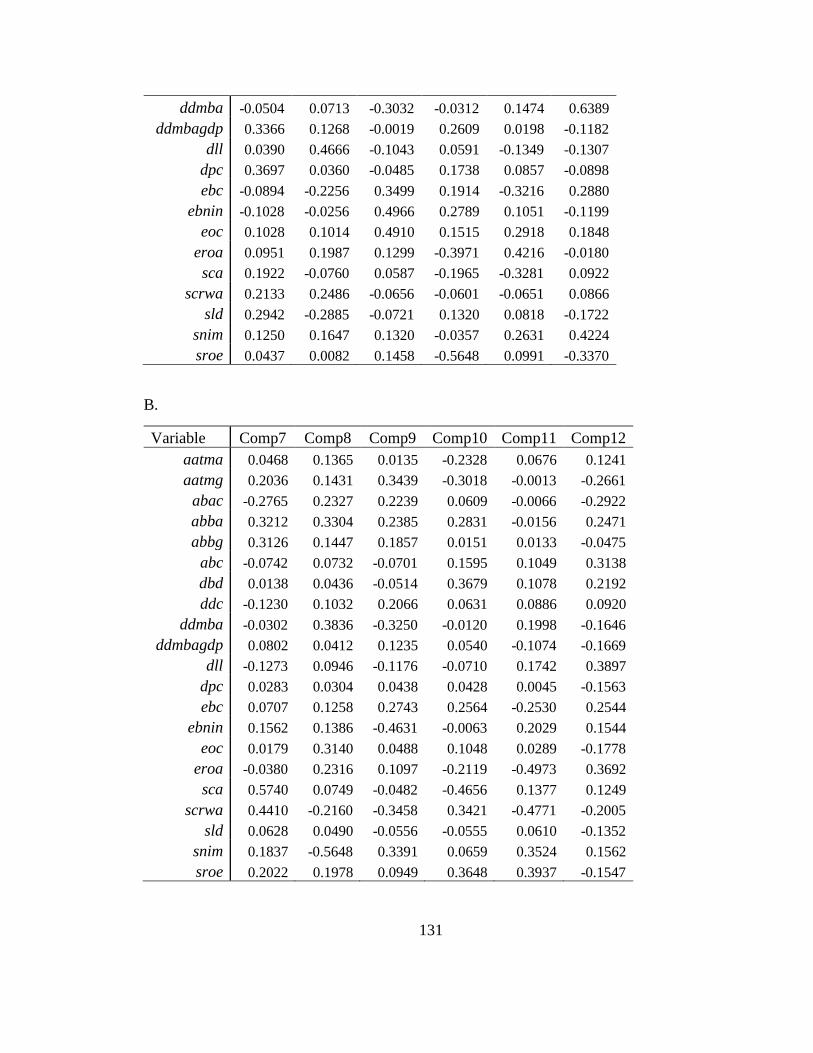
131
ddmba -0.0504 0.0713 -0.3032 -0.0312 0.1474 0.6389
ddmbagdp 0.3366 0.1268 -0.0019 0.2609 0.0198 -0.1182
dll 0.0390 0.4666 -0.1043 0.0591 -0.1349 -0.1307
dpc 0.3697 0.0360 -0.0485 0.1738 0.0857 -0.0898
ebc -0.0894 -0.2256 0.3499 0.1914 -0.3216 0.2880
ebnin -0.1028 -0.0256 0.4966 0.2789 0.1051 -0.1199
eoc 0.1028 0.1014 0.4910 0.1515 0.2918 0.1848
eroa 0.0951 0.1987 0.1299 -0.3971 0.4216 -0.0180
sca 0.1922 -0.0760 0.0587 -0.1965 -0.3281 0.0922
scrwa 0.2133 0.2486 -0.0656 -0.0601 -0.0651 0.0866
sld 0.2942 -0.2885 -0.0721 0.1320 0.0818 -0.1722
snim 0.1250 0.1647 0.1320 -0.0357 0.2631 0.4224
sroe 0.0437 0.0082 0.1458 -0.5648 0.0991 -0.3370
B.
Variable Comp7 Comp8 Comp9 Comp10 Comp11 Comp12
aatma 0.0468 0.1365 0.0135 -0.2328 0.0676 0.1241
aatmg 0.2036 0.1431 0.3439 -0.3018 -0.0013 -0.2661
abac -0.2765 0.2327 0.2239 0.0609 -0.0066 -0.2922
abba 0.3212 0.3304 0.2385 0.2831 -0.0156 0.2471
abbg 0.3126 0.1447 0.1857 0.0151 0.0133 -0.0475
abc -0.0742 0.0732 -0.0701 0.1595 0.1049 0.3138
dbd 0.0138 0.0436 -0.0514 0.3679 0.1078 0.2192
ddc -0.1230 0.1032 0.2066 0.0631 0.0886 0.0920
ddmba -0.0302 0.3836 -0.3250 -0.0120 0.1998 -0.1646
ddmbagdp 0.0802 0.0412 0.1235 0.0540 -0.1074 -0.1669
dll -0.1273 0.0946 -0.1176 -0.0710 0.1742 0.3897
dpc 0.0283 0.0304 0.0438 0.0428 0.0045 -0.1563
ebc 0.0707 0.1258 0.2743 0.2564 -0.2530 0.2544
ebnin 0.1562 0.1386 -0.4631 -0.0063 0.2029 0.1544
eoc 0.0179 0.3140 0.0488 0.1048 0.0289 -0.1778
eroa -0.0380 0.2316 0.1097 -0.2119 -0.4973 0.3692
sca 0.5740 0.0749 -0.0482 -0.4656 0.1377 0.1249
scrwa 0.4410 -0.2160 -0.3458 0.3421 -0.4771 -0.2005
sld 0.0628 0.0490 -0.0556 -0.0555 0.0610 -0.1352
snim 0.1837 -0.5648 0.3391 0.0659 0.3524 0.1562
sroe 0.2022 0.1978 0.0949 0.3648 0.3937 -0.1547
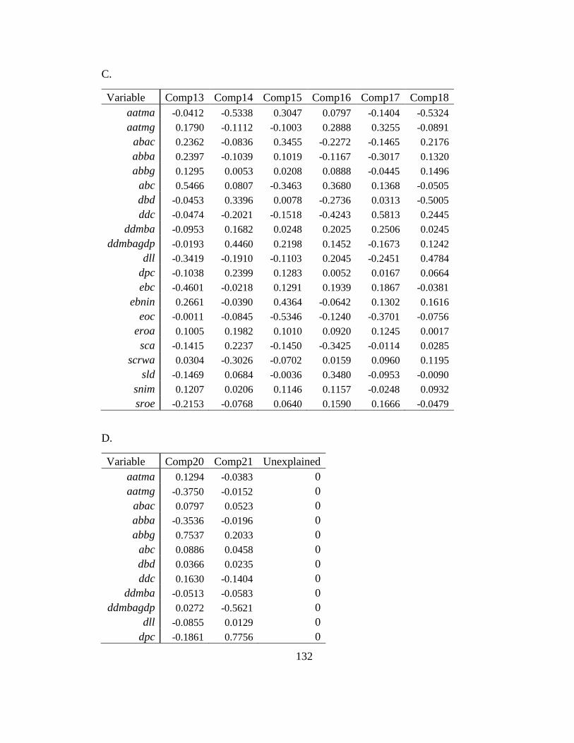
132
C.
Variable Comp13 Comp14 Comp15 Comp16 Comp17 Comp18
aatma -0.0412 -0.5338 0.3047 0.0797 -0.1404 -0.5324
aatmg 0.1790 -0.1112 -0.1003 0.2888 0.3255 -0.0891
abac 0.2362 -0.0836 0.3455 -0.2272 -0.1465 0.2176
abba 0.2397 -0.1039 0.1019 -0.1167 -0.3017 0.1320
abbg 0.1295 0.0053 0.0208 0.0888 -0.0445 0.1496
abc 0.5466 0.0807 -0.3463 0.3680 0.1368 -0.0505
dbd -0.0453 0.3396 0.0078 -0.2736 0.0313 -0.5005
ddc -0.0474 -0.2021 -0.1518 -0.4243 0.5813 0.2445
ddmba -0.0953 0.1682 0.0248 0.2025 0.2506 0.0245
ddmbagdp -0.0193 0.4460 0.2198 0.1452 -0.1673 0.1242
dll -0.3419 -0.1910 -0.1103 0.2045 -0.2451 0.4784
dpc -0.1038 0.2399 0.1283 0.0052 0.0167 0.0664
ebc -0.4601 -0.0218 0.1291 0.1939 0.1867 -0.0381
ebnin 0.2661 -0.0390 0.4364 -0.0642 0.1302 0.1616
eoc -0.0011 -0.0845 -0.5346 -0.1240 -0.3701 -0.0756
eroa 0.1005 0.1982 0.1010 0.0920 0.1245 0.0017
sca -0.1415 0.2237 -0.1450 -0.3425 -0.0114 0.0285
scrwa 0.0304 -0.3026 -0.0702 0.0159 0.0960 0.1195
sld -0.1469 0.0684 -0.0036 0.3480 -0.0953 -0.0090
snim 0.1207 0.0206 0.1146 0.1157 -0.0248 0.0932
sroe -0.2153 -0.0768 0.0640 0.1590 0.1666 -0.0479
D.
Variable Comp20 Comp21 Unexplained
aatma 0.1294 -0.0383 0
aatmg -0.3750 -0.0152 0
abac 0.0797 0.0523 0
abba -0.3536 -0.0196 0
abbg 0.7537 0.2033 0
abc 0.0886 0.0458 0
dbd 0.0366 0.0235 0
ddc 0.1630 -0.1404 0
ddmba -0.0513 -0.0583 0
ddmbagdp 0.0272 -0.5621 0
dll -0.0855 0.0129 0
dpc -0.1861 0.7756 0
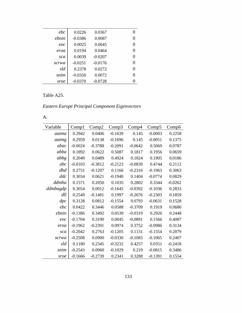
133
ebc 0.0226 0.0367 0
ebnin -0.0386 0.0087 0
eoc 0.0025 0.0045 0
eroa 0.0194 0.0464 0
sca 0.0039 -0.0207 0
scrwa -0.0251 -0.0176 0
sld 0.2378 0.0272 0
snim -0.0350 0.0072 0
sroe -0.0370 -0.0728 0
Table A25.
Eastern Europe Principal Component Eigenvectors
A.
Variable Comp1 Comp2 Comp3 Comp4 Comp5 Comp6
aatma 0.2942 0.0406 -0.1639 0.145 -0.0003 0.2258
aatmg 0.2959 0.0138 -0.1696 0.145 -0.0051 0.1375
abac -0.0024 -0.3788 -0.2091 -0.0642 0.5069 0.0787
abba 0.1892 0.0622 0.5087 0.1817 0.1956 0.0659
abbg 0.2049 0.0489 0.4924 0.1824 0.1905 0.0186
abc -0.0103 -0.3812 -0.2123 -0.0839 0.4744 0.2112
dbd 0.2751 -0.1207 0.1166 -0.2316 -0.1963 0.3063
ddc 0.3034 0.0621 -0.1940 0.1404 -0.0774 0.0829
ddmba 0.1571 0.2050 0.1035 0.2802 0.3344 -0.0262
ddmbagdp 0.3054 0.0012 -0.1645 -0.0392 -0.1036 0.2833
dll 0.2549 -0.1481 0.1997 -0.2676 -0.2303 0.1859
dpc 0.3128 0.0812 -0.1554 0.0793 -0.0631 0.1528
ebc 0.0422 0.3446 0.0588 -0.3709 0.1919 0.0680
ebnin -0.1386 0.3492 0.0539 -0.0319 0.2926 0.2448
eoc -0.1704 0.3190 0.0045 -0.0891 0.1566 0.4087
eroa -0.1962 -0.2391 0.0974 0.3752 -0.0986 0.3134
sca -0.2042 0.2763 -0.1205 0.1131 -0.1554 0.2079
scrwa -0.2508 0.0900 -0.0330 -0.1083 -0.1065 0.2407
sld 0.1180 0.2345 -0.3232 0.4257 0.0351 -0.2418
snim -0.2543 0.0060 -0.1029 0.219 -0.0815 0.3486
sroe -0.1666 -0.2739 0.2341 0.3288 -0.1391 0.1554
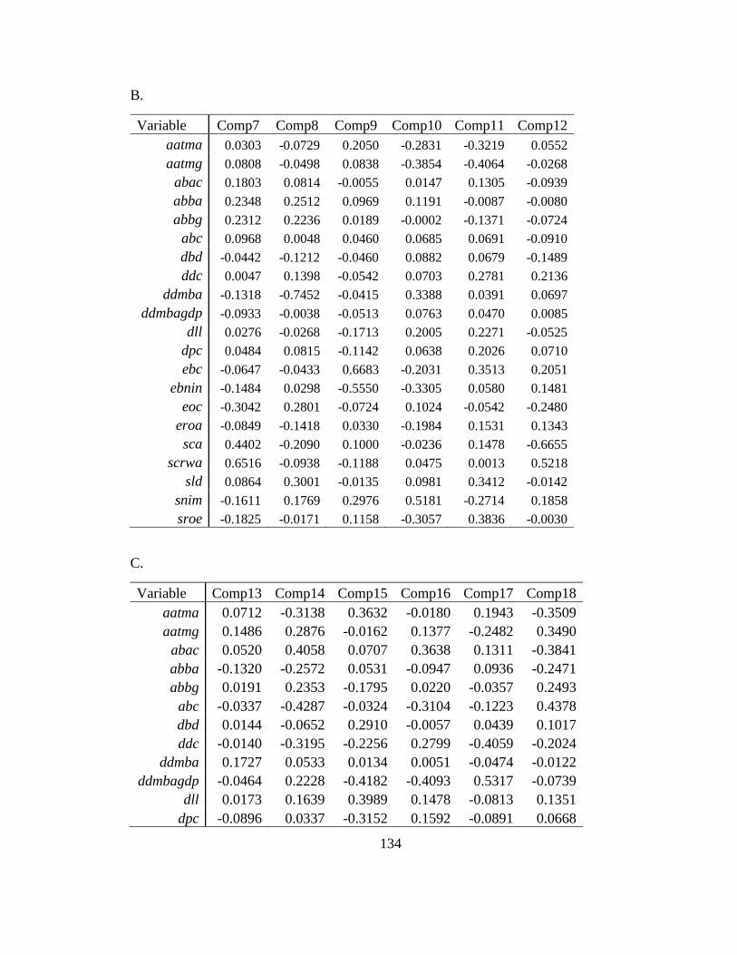
134
B.
Variable Comp7 Comp8 Comp9 Comp10 Comp11 Comp12
aatma 0.0303 -0.0729 0.2050 -0.2831 -0.3219 0.0552
aatmg 0.0808 -0.0498 0.0838 -0.3854 -0.4064 -0.0268
abac 0.1803 0.0814 -0.0055 0.0147 0.1305 -0.0939
abba 0.2348 0.2512 0.0969 0.1191 -0.0087 -0.0080
abbg 0.2312 0.2236 0.0189 -0.0002 -0.1371 -0.0724
abc 0.0968 0.0048 0.0460 0.0685 0.0691 -0.0910
dbd -0.0442 -0.1212 -0.0460 0.0882 0.0679 -0.1489
ddc 0.0047 0.1398 -0.0542 0.0703 0.2781 0.2136
ddmba -0.1318 -0.7452 -0.0415 0.3388 0.0391 0.0697
ddmbagdp -0.0933 -0.0038 -0.0513 0.0763 0.0470 0.0085
dll 0.0276 -0.0268 -0.1713 0.2005 0.2271 -0.0525
dpc 0.0484 0.0815 -0.1142 0.0638 0.2026 0.0710
ebc -0.0647 -0.0433 0.6683 -0.2031 0.3513 0.2051
ebnin -0.1484 0.0298 -0.5550 -0.3305 0.0580 0.1481
eoc -0.3042 0.2801 -0.0724 0.1024 -0.0542 -0.2480
eroa -0.0849 -0.1418 0.0330 -0.1984 0.1531 0.1343
sca 0.4402 -0.2090 0.1000 -0.0236 0.1478 -0.6655
scrwa 0.6516 -0.0938 -0.1188 0.0475 0.0013 0.5218
sld 0.0864 0.3001 -0.0135 0.0981 0.3412 -0.0142
snim -0.1611 0.1769 0.2976 0.5181 -0.2714 0.1858
sroe -0.1825 -0.0171 0.1158 -0.3057 0.3836 -0.0030
C.
Variable Comp13 Comp14 Comp15 Comp16 Comp17 Comp18
aatma 0.0712 -0.3138 0.3632 -0.0180 0.1943 -0.3509
aatmg 0.1486 0.2876 -0.0162 0.1377 -0.2482 0.3490
abac 0.0520 0.4058 0.0707 0.3638 0.1311 -0.3841
abba -0.1320 -0.2572 0.0531 -0.0947 0.0936 -0.2471
abbg 0.0191 0.2353 -0.1795 0.0220 -0.0357 0.2493
abc -0.0337 -0.4287 -0.0324 -0.3104 -0.1223 0.4378
dbd 0.0144 -0.0652 0.2910 -0.0057 0.0439 0.1017
ddc -0.0140 -0.3195 -0.2256 0.2799 -0.4059 -0.2024
ddmba 0.1727 0.0533 0.0134 0.0051 -0.0474 -0.0122
ddmbagdp -0.0464 0.2228 -0.4182 -0.4093 0.5317 -0.0739
dll 0.0173 0.1639 0.3989 0.1478 -0.0813 0.1351
dpc -0.0896 0.0337 -0.3152 0.1592 -0.0891 0.0668
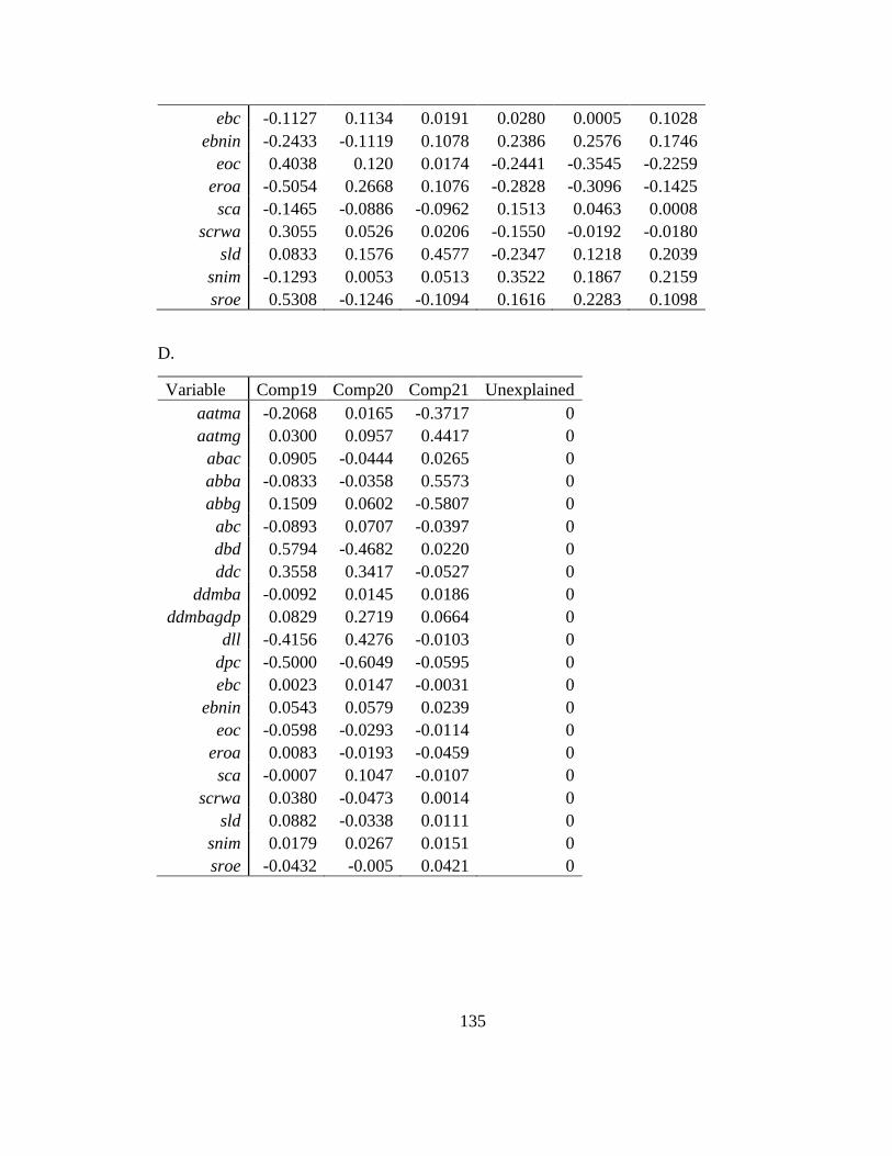
135
ebc -0.1127 0.1134 0.0191 0.0280 0.0005 0.1028
ebnin -0.2433 -0.1119 0.1078 0.2386 0.2576 0.1746
eoc 0.4038 0.120 0.0174 -0.2441 -0.3545 -0.2259
eroa -0.5054 0.2668 0.1076 -0.2828 -0.3096 -0.1425
sca -0.1465 -0.0886 -0.0962 0.1513 0.0463 0.0008
scrwa 0.3055 0.0526 0.0206 -0.1550 -0.0192 -0.0180
sld 0.0833 0.1576 0.4577 -0.2347 0.1218 0.2039
snim -0.1293 0.0053 0.0513 0.3522 0.1867 0.2159
sroe 0.5308 -0.1246 -0.1094 0.1616 0.2283 0.1098
D.
Variable Comp19 Comp20 Comp21 Unexplained
aatma -0.2068 0.0165 -0.3717 0
aatmg 0.0300 0.0957 0.4417 0
abac 0.0905 -0.0444 0.0265 0
abba -0.0833 -0.0358 0.5573 0
abbg 0.1509 0.0602 -0.5807 0
abc -0.0893 0.0707 -0.0397 0
dbd 0.5794 -0.4682 0.0220 0
ddc 0.3558 0.3417 -0.0527 0
ddmba -0.0092 0.0145 0.0186 0
ddmbagdp 0.0829 0.2719 0.0664 0
dll -0.4156 0.4276 -0.0103 0
dpc -0.5000 -0.6049 -0.0595 0
ebc 0.0023 0.0147 -0.0031 0
ebnin 0.0543 0.0579 0.0239 0
eoc -0.0598 -0.0293 -0.0114 0
eroa 0.0083 -0.0193 -0.0459 0
sca -0.0007 0.1047 -0.0107 0
scrwa 0.0380 -0.0473 0.0014 0
sld 0.0882 -0.0338 0.0111 0
snim 0.0179 0.0267 0.0151 0
sroe -0.0432 -0.005 0.0421 0
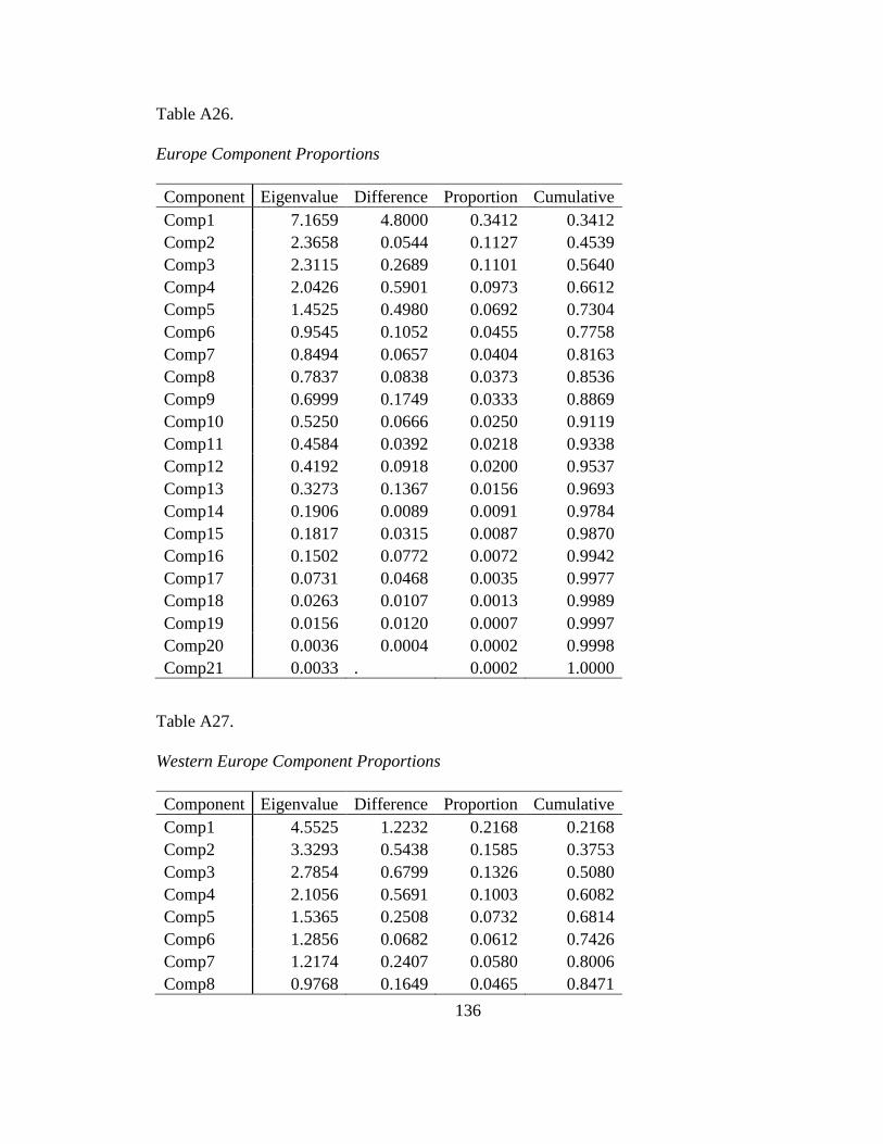
136
Table A26.
Europe Component Proportions
Component Eigenvalue Difference Proportion Cumulative
Comp1 7.1659 4.8000 0.3412 0.3412
Comp2 2.3658 0.0544 0.1127 0.4539
Comp3 2.3115 0.2689 0.1101 0.5640
Comp4 2.0426 0.5901 0.0973 0.6612
Comp5 1.4525 0.4980 0.0692 0.7304
Comp6 0.9545 0.1052 0.0455 0.7758
Comp7 0.8494 0.0657 0.0404 0.8163
Comp8 0.7837 0.0838 0.0373 0.8536
Comp9 0.6999 0.1749 0.0333 0.8869
Comp10 0.5250 0.0666 0.0250 0.9119
Comp11 0.4584 0.0392 0.0218 0.9338
Comp12 0.4192 0.0918 0.0200 0.9537
Comp13 0.3273 0.1367 0.0156 0.9693
Comp14 0.1906 0.0089 0.0091 0.9784
Comp15 0.1817 0.0315 0.0087 0.9870
Comp16 0.1502 0.0772 0.0072 0.9942
Comp17 0.0731 0.0468 0.0035 0.9977
Comp18 0.0263 0.0107 0.0013 0.9989
Comp19 0.0156 0.0120 0.0007 0.9997
Comp20 0.0036 0.0004 0.0002 0.9998
Comp21 0.0033 . 0.0002 1.0000
Table A27.
Western Europe Component Proportions
Component Eigenvalue Difference Proportion Cumulative
Comp1 4.5525 1.2232 0.2168 0.2168
Comp2 3.3293 0.5438 0.1585 0.3753
Comp3 2.7854 0.6799 0.1326 0.5080
Comp4 2.1056 0.5691 0.1003 0.6082
Comp5 1.5365 0.2508 0.0732 0.6814
Comp6 1.2856 0.0682 0.0612 0.7426
Comp7 1.2174 0.2407 0.0580 0.8006
Comp8 0.9768 0.1649 0.0465 0.8471
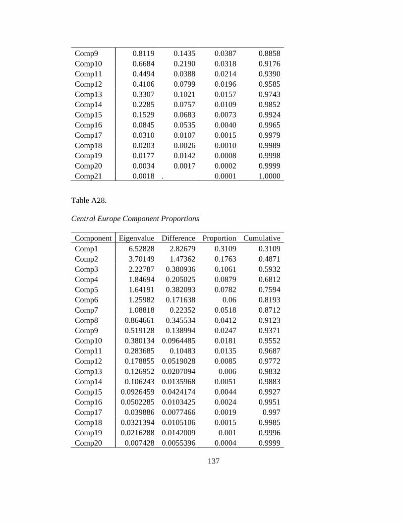
137
Comp9 0.8119 0.1435 0.0387 0.8858
Comp10 0.6684 0.2190 0.0318 0.9176
Comp11 0.4494 0.0388 0.0214 0.9390
Comp12 0.4106 0.0799 0.0196 0.9585
Comp13 0.3307 0.1021 0.0157 0.9743
Comp14 0.2285 0.0757 0.0109 0.9852
Comp15 0.1529 0.0683 0.0073 0.9924
Comp16 0.0845 0.0535 0.0040 0.9965
Comp17 0.0310 0.0107 0.0015 0.9979
Comp18 0.0203 0.0026 0.0010 0.9989
Comp19 0.0177 0.0142 0.0008 0.9998
Comp20 0.0034 0.0017 0.0002 0.9999
Comp21 0.0018 . 0.0001 1.0000
Table A28.
Central Europe Component Proportions
Component Eigenvalue Difference Proportion Cumulative
Comp1 6.52828 2.82679 0.3109 0.3109
Comp2 3.70149 1.47362 0.1763 0.4871
Comp3 2.22787 0.380936 0.1061 0.5932
Comp4 1.84694 0.205025 0.0879 0.6812
Comp5 1.64191 0.382093 0.0782 0.7594
Comp6 1.25982 0.171638 0.06 0.8193
Comp7 1.08818 0.22352 0.0518 0.8712
Comp8 0.864661 0.345534 0.0412 0.9123
Comp9 0.519128 0.138994 0.0247 0.9371
Comp10 0.380134 0.0964485 0.0181 0.9552
Comp11 0.283685 0.10483 0.0135 0.9687
Comp12 0.178855 0.0519028 0.0085 0.9772
Comp13 0.126952 0.0207094 0.006 0.9832
Comp14 0.106243 0.0135968 0.0051 0.9883
Comp15 0.0926459 0.0424174 0.0044 0.9927
Comp16 0.0502285 0.0103425 0.0024 0.9951
Comp17 0.039886 0.0077466 0.0019 0.997
Comp18 0.0321394 0.0105106 0.0015 0.9985
Comp19 0.0216288 0.0142009 0.001 0.9996
Comp20 0.007428 0.0055396 0.0004 0.9999
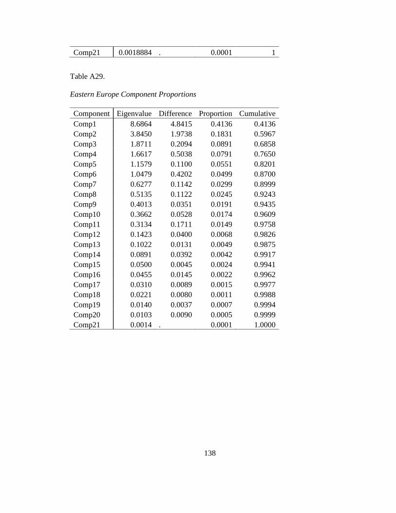
138
Comp21 0.0018884 . 0.0001 1
Table A29.
Eastern Europe Component Proportions
Component Eigenvalue Difference Proportion Cumulative
Comp1 8.6864 4.8415 0.4136 0.4136
Comp2 3.8450 1.9738 0.1831 0.5967
Comp3 1.8711 0.2094 0.0891 0.6858
Comp4 1.6617 0.5038 0.0791 0.7650
Comp5 1.1579 0.1100 0.0551 0.8201
Comp6 1.0479 0.4202 0.0499 0.8700
Comp7 0.6277 0.1142 0.0299 0.8999
Comp8 0.5135 0.1122 0.0245 0.9243
Comp9 0.4013 0.0351 0.0191 0.9435
Comp10 0.3662 0.0528 0.0174 0.9609
Comp11 0.3134 0.1711 0.0149 0.9758
Comp12 0.1423 0.0400 0.0068 0.9826
Comp13 0.1022 0.0131 0.0049 0.9875
Comp14 0.0891 0.0392 0.0042 0.9917
Comp15 0.0500 0.0045 0.0024 0.9941
Comp16 0.0455 0.0145 0.0022 0.9962
Comp17 0.0310 0.0089 0.0015 0.9977
Comp18 0.0221 0.0080 0.0011 0.9988
Comp19 0.0140 0.0037 0.0007 0.9994
Comp20 0.0103 0.0090 0.0005 0.9999
Comp21 0.0014 . 0.0001 1.0000
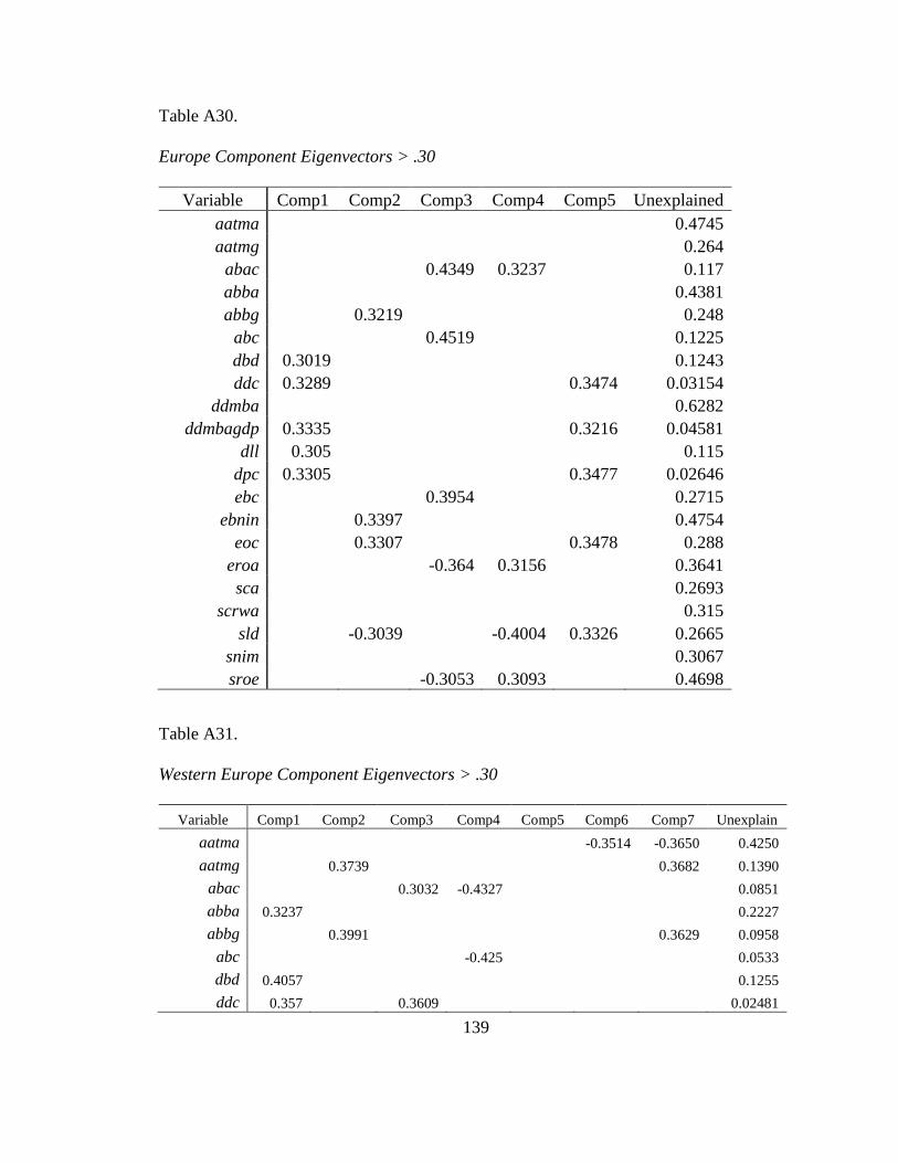
139
Table A30.
Europe Component Eigenvectors > .30
Variable Comp1 Comp2 Comp3 Comp4 Comp5 Unexplained
aatma 0.4745
aatmg 0.264
abac 0.4349 0.3237 0.117
abba 0.4381
abbg 0.3219 0.248
abc 0.4519 0.1225
dbd 0.3019 0.1243
ddc 0.3289 0.3474 0.03154
ddmba 0.6282
ddmbagdp 0.3335 0.3216 0.04581
dll 0.305 0.115
dpc 0.3305 0.3477 0.02646
ebc 0.3954 0.2715
ebnin 0.3397 0.4754
eoc 0.3307 0.3478 0.288
eroa -0.364 0.3156 0.3641
sca 0.2693
scrwa 0.315
sld -0.3039 -0.4004 0.3326 0.2665
snim 0.3067
sroe -0.3053 0.3093 0.4698
Table A31.
Western Europe Component Eigenvectors > .30
Variable Comp1 Comp2 Comp3 Comp4 Comp5 Comp6 Comp7 Unexplain
aatma -0.3514 -0.3650 0.4250
aatmg 0.3739 0.3682 0.1390
abac 0.3032 -0.4327 0.0851
abba 0.3237 0.2227
abbg 0.3991 0.3629 0.0958
abc -0.425 0.0533
dbd 0.4057 0.1255
ddc 0.357 0.3609 0.02481
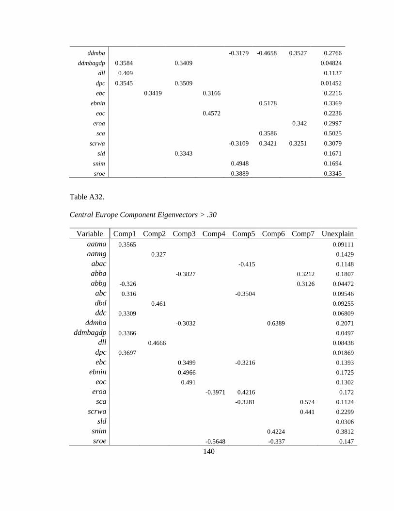
140
ddmba -0.3179 -0.4658 0.3527 0.2766
ddmbagdp 0.3584 0.3409 0.04824
dll 0.409 0.1137
dpc 0.3545 0.3509 0.01452
ebc 0.3419 0.3166 0.2216
ebnin 0.5178 0.3369
eoc 0.4572 0.2236
eroa 0.342 0.2997
sca 0.3586 0.5025
scrwa -0.3109 0.3421 0.3251 0.3079
sld 0.3343 0.1671
snim 0.4948 0.1694
sroe 0.3889 0.3345
Table A32.
Central Europe Component Eigenvectors > .30
Variable Comp1 Comp2 Comp3 Comp4 Comp5 Comp6 Comp7 Unexplain
aatma 0.3565 0.09111
aatmg 0.327 0.1429
abac -0.415 0.1148
abba -0.3827 0.3212 0.1807
abbg -0.326 0.3126 0.04472
abc 0.316 -0.3504 0.09546
dbd 0.461 0.09255
ddc 0.3309 0.06809
ddmba -0.3032 0.6389 0.2071
ddmbagdp 0.3366 0.0497
dll 0.4666 0.08438
dpc 0.3697 0.01869
ebc 0.3499 -0.3216 0.1393
ebnin 0.4966 0.1725
eoc 0.491 0.1302
eroa -0.3971 0.4216 0.172
sca -0.3281 0.574 0.1124
scrwa 0.441 0.2299
sld 0.0306
snim 0.4224 0.3812
sroe -0.5648 -0.337 0.147
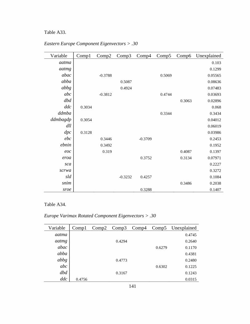
141
Table A33.
Eastern Europe Component Eigenvectors > .30
Variable Comp1 Comp2 Comp3 Comp4 Comp5 Comp6 Unexplained
aatma 0.103
aatmg 0.1299
abac -0.3788 0.5069 0.05565
abba 0.5087 0.08636
abbg 0.4924 0.07483
abc -0.3812 0.4744 0.03693
dbd 0.3063 0.02896
ddc 0.3034 0.068
ddmba 0.3344 0.3434
ddmbagdp 0.3054 0.04012
dll 0.06019
dpc 0.3128 0.03986
ebc 0.3446 -0.3709 0.2453
ebnin 0.3492 0.1952
eoc 0.319 0.4087 0.1397
eroa 0.3752 0.3134 0.07971
sca 0.2227
scrwa 0.3272
sld -0.3232 0.4257 0.1084
snim 0.3486 0.2038
sroe 0.3288 0.1407
Table A34.
Europe Varimax Rotated Component Eigenvectors > .30
Variable Comp1 Comp2 Comp3 Comp4 Comp5 Unexplained
aatma 0.4745
aatmg 0.4294 0.2640
abac 0.6279 0.1170
abba 0.4381
abbg 0.4773 0.2480
abc 0.6302 0.1225
dbd 0.3167 0.1243
ddc 0.4756 0.0315
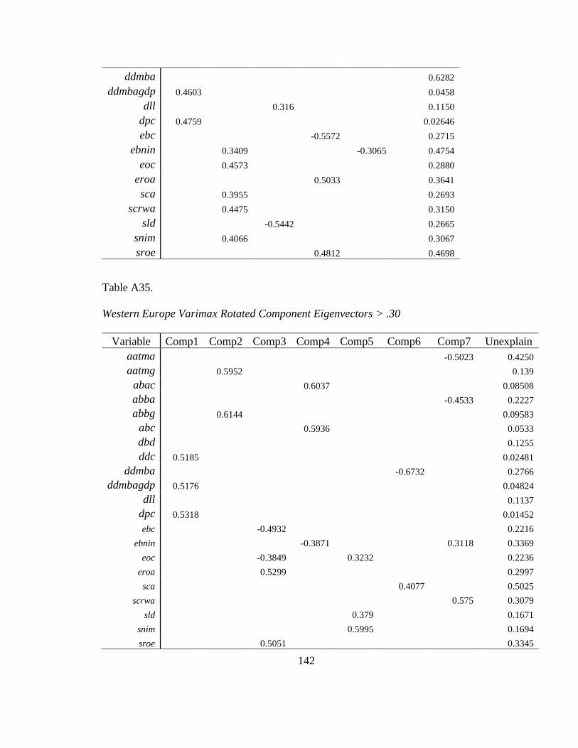
142
ddmba 0.6282
ddmbagdp 0.4603 0.0458
dll 0.316 0.1150
dpc 0.4759 0.02646
ebc -0.5572 0.2715
ebnin 0.3409 -0.3065 0.4754
eoc 0.4573 0.2880
eroa 0.5033 0.3641
sca 0.3955 0.2693
scrwa 0.4475 0.3150
sld -0.5442 0.2665
snim 0.4066 0.3067
sroe 0.4812 0.4698
Table A35.
Western Europe Varimax Rotated Component Eigenvectors > .30
Variable Comp1 Comp2 Comp3 Comp4 Comp5 Comp6 Comp7 Unexplain
aatma -0.5023 0.4250
aatmg 0.5952 0.139
abac 0.6037 0.08508
abba -0.4533 0.2227
abbg 0.6144 0.09583
abc 0.5936 0.0533
dbd 0.1255
ddc 0.5185 0.02481
ddmba -0.6732 0.2766
ddmbagdp 0.5176 0.04824
dll 0.1137
dpc 0.5318 0.01452
ebc -0.4932 0.2216
ebnin -0.3871 0.3118 0.3369
eoc -0.3849 0.3232 0.2236
eroa 0.5299 0.2997
sca 0.4077 0.5025
scrwa 0.575 0.3079
sld 0.379 0.1671
snim 0.5995 0.1694
sroe 0.5051 0.3345
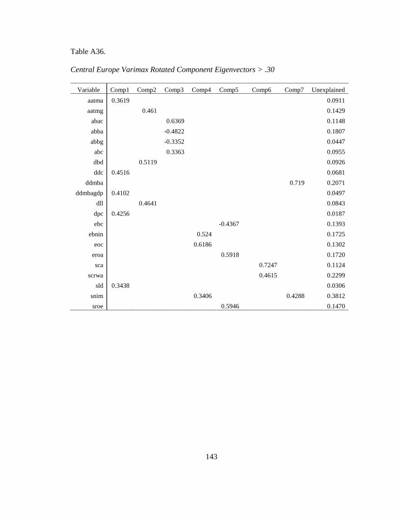
143
Table A36.
Central Europe Varimax Rotated Component Eigenvectors > .30
Variable Comp1 Comp2 Comp3 Comp4 Comp5 Comp6 Comp7 Unexplained
aatma 0.3619 0.0911
aatmg 0.461 0.1429
abac 0.6369 0.1148
abba -0.4822 0.1807
abbg -0.3352 0.0447
abc 0.3363 0.0955
dbd 0.5119 0.0926
ddc 0.4516 0.0681
ddmba 0.719 0.2071
ddmbagdp 0.4102 0.0497
dll 0.4641 0.0843
dpc 0.4256 0.0187
ebc -0.4367 0.1393
ebnin 0.524 0.1725
eoc 0.6186 0.1302
eroa 0.5918 0.1720
sca 0.7247 0.1124
scrwa 0.4615 0.2299
sld 0.3438 0.0306
snim 0.3406 0.4288 0.3812
sroe 0.5946 0.1470
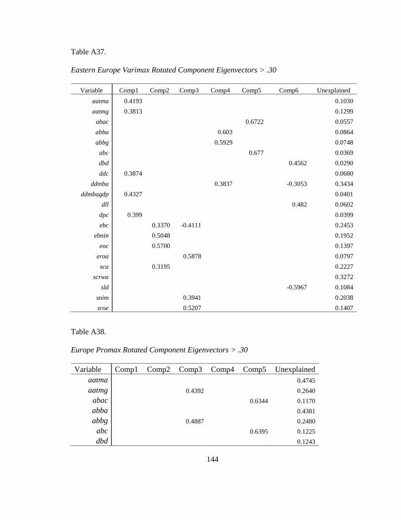
144
Table A37.
Eastern Europe Varimax Rotated Component Eigenvectors > .30
Variable Comp1 Comp2 Comp3 Comp4 Comp5 Comp6 Unexplained
aatma 0.4193 0.1030
aatmg 0.3813 0.1299
abac 0.6722 0.0557
abba 0.603 0.0864
abbg 0.5929 0.0748
abc 0.677 0.0369
dbd 0.4562 0.0290
ddc 0.3874 0.0680
ddmba 0.3837 -0.3053 0.3434
ddmbagdp 0.4327 0.0401
dll 0.482 0.0602
dpc 0.399 0.0399
ebc 0.3370 -0.4111 0.2453
ebnin 0.5048 0.1952
eoc 0.5700 0.1397
eroa 0.5878 0.0797
sca 0.3195 0.2227
scrwa 0.3272
sld -0.5967 0.1084
snim 0.3941 0.2038
sroe 0.5207 0.1407
Table A38.
Europe Promax Rotated Component Eigenvectors > .30
Variable Comp1 Comp2 Comp3 Comp4 Comp5 Unexplained
aatma 0.4745
aatmg 0.4392 0.2640
abac 0.6344 0.1170
abba 0.4381
abbg 0.4887 0.2480
abc 0.6395 0.1225
dbd 0.1243
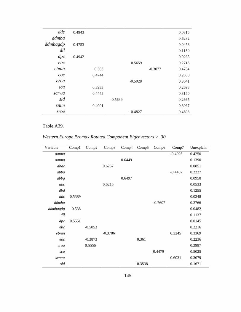
145
ddc 0.4943 0.0315
ddmba 0.6282
ddmbagdp 0.4753 0.0458
dll 0.1150
dpc 0.4942 0.0265
ebc 0.5659 0.2715
ebnin 0.363 -0.3077 0.4754
eoc 0.4744 0.2880
eroa -0.5028 0.3641
sca 0.3933 0.2693
scrwa 0.4445 0.3150
sld -0.5639 0.2665
snim 0.4001 0.3067
sroe -0.4827 0.4698
Table A39.
Western Europe Promax Rotated Component Eigenvectors > .30
Variable Comp1 Comp2 Comp3 Comp4 Comp5 Comp6 Comp7 Unexplain
aatma
-0.4995 0.4250
aatmg
0.6449
0.1390
abac
0.6257
0.0851
abba
-0.4407 0.2227
abbg
0.6497
0.0958
abc
0.6215
0.0533
dbd
0.1255
ddc 0.5389
0.0248
ddmba
-0.7607
0.2766
ddmbagdp 0.538
0.0482
dll
0.1137
dpc 0.5551
0.0145
ebc
-0.5053
0.2216
ebnin
-0.3786
0.3245 0.3369
eoc
-0.3873
0.361
0.2236
eroa
0.5556
0.2997
sca
0.4479
0.5025
scrwa
0.6031 0.3079
sld
0.3538
0.1671
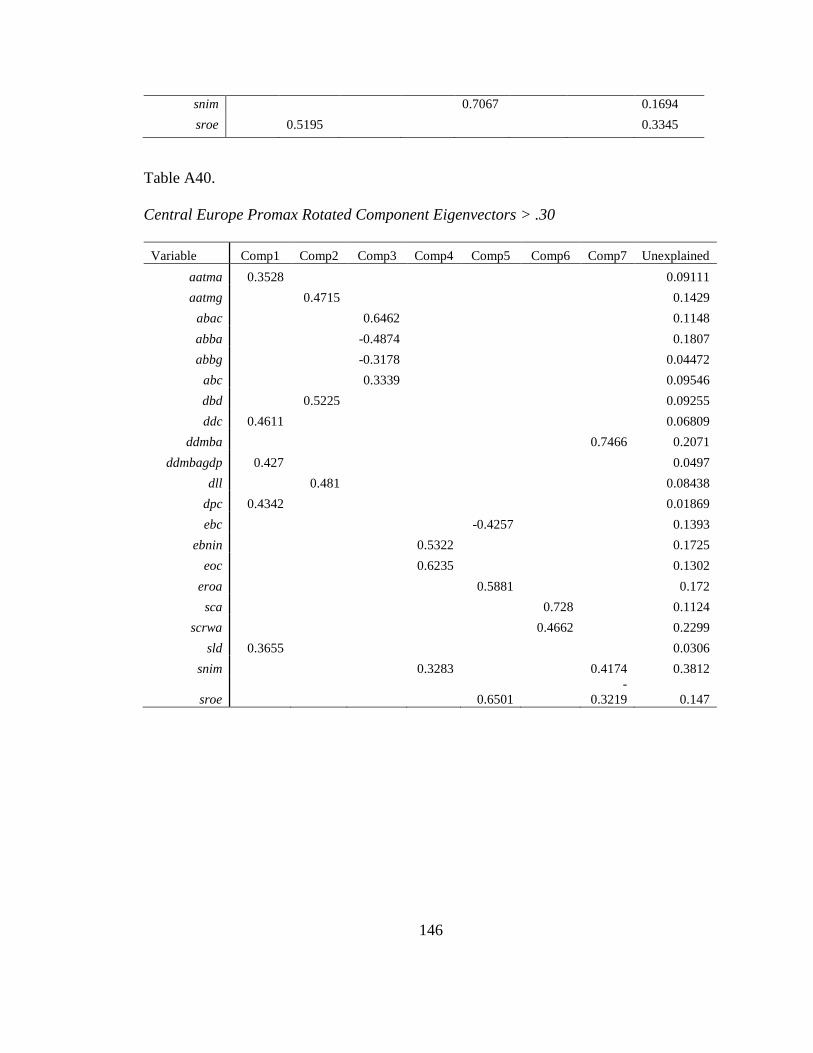
146
snim
0.7067
0.1694
sroe
0.5195
0.3345
Table A40.
Central Europe Promax Rotated Component Eigenvectors > .30
Variable Comp1 Comp2 Comp3 Comp4 Comp5 Comp6 Comp7 Unexplained
aatma 0.3528 0.09111
aatmg 0.4715 0.1429
abac 0.6462 0.1148
abba -0.4874 0.1807
abbg -0.3178 0.04472
abc 0.3339 0.09546
dbd 0.5225 0.09255
ddc 0.4611 0.06809
ddmba 0.7466 0.2071
ddmbagdp 0.427 0.0497
dll 0.481 0.08438
dpc 0.4342 0.01869
ebc -0.4257 0.1393
ebnin 0.5322 0.1725
eoc 0.6235 0.1302
eroa 0.5881 0.172
sca 0.728 0.1124
scrwa 0.4662 0.2299
sld 0.3655 0.0306
snim 0.3283 0.4174 0.3812
sroe 0.6501
-
0.3219 0.147
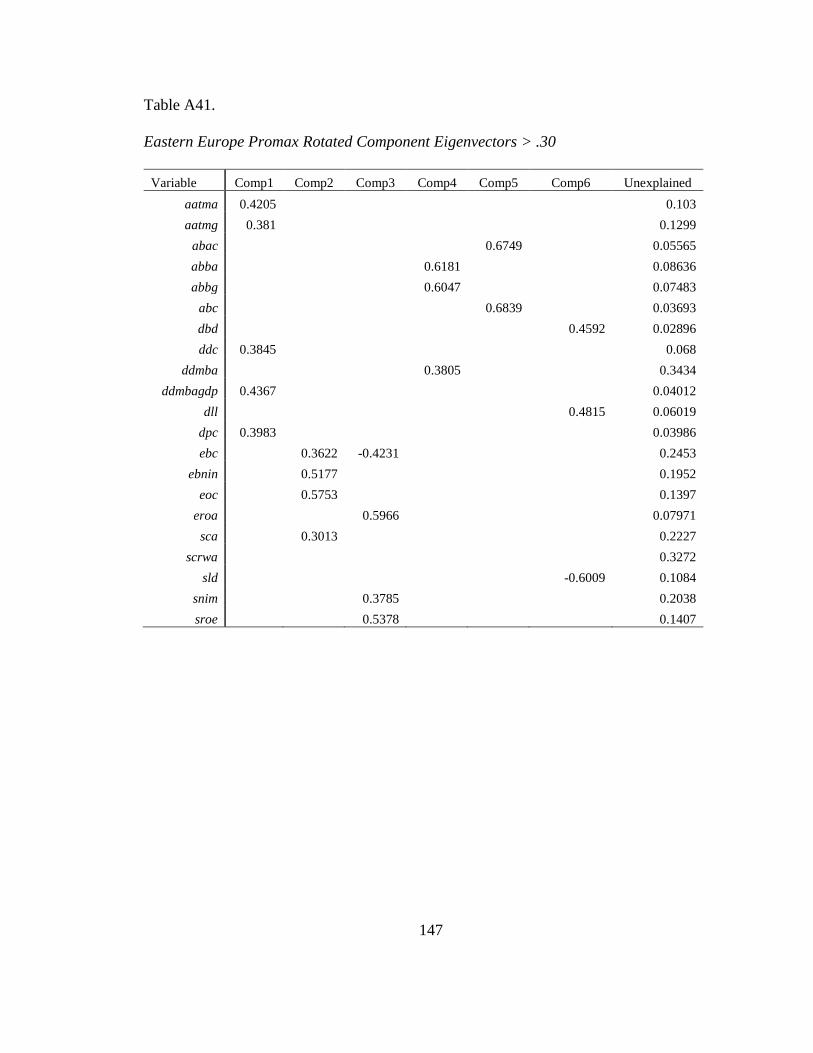
147
Table A41.
Eastern Europe Promax Rotated Component Eigenvectors > .30
Variable Comp1 Comp2 Comp3 Comp4 Comp5 Comp6 Unexplained
aatma 0.4205 0.103
aatmg 0.381 0.1299
abac 0.6749 0.05565
abba 0.6181 0.08636
abbg 0.6047 0.07483
abc 0.6839 0.03693
dbd 0.4592 0.02896
ddc 0.3845 0.068
ddmba 0.3805 0.3434
ddmbagdp 0.4367 0.04012
dll 0.4815 0.06019
dpc 0.3983 0.03986
ebc 0.3622 -0.4231 0.2453
ebnin 0.5177 0.1952
eoc 0.5753 0.1397
eroa 0.5966 0.07971
sca 0.3013 0.2227
scrwa 0.3272
sld -0.6009 0.1084
snim 0.3785 0.2038
sroe 0.5378 0.1407
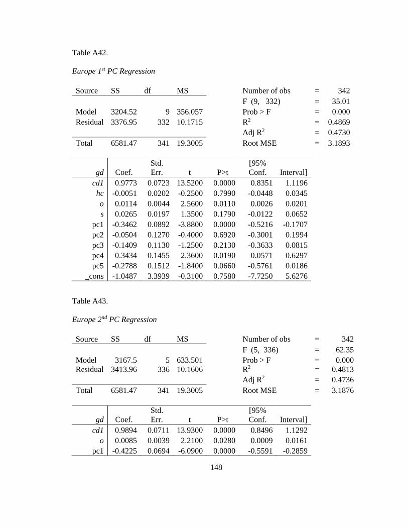
148
Table A42.
Europe 1st PC Regression
Source SS df MS Number of obs = 342
F (9, 332) = 35.01
Model 3204.52 9 356.057 Prob > F = 0.000
Residual 3376.95 332 10.1715 R2 = 0.4869
Adj R2 = 0.4730
Total 6581.47 341 19.3005 Root MSE = 3.1893
gd Coef.
Std.
Err. t P>t
[95%
Conf. Interval]
cd1 0.9773 0.0723 13.5200 0.0000 0.8351 1.1196
hc -0.0051 0.0202 -0.2500 0.7990 -0.0448 0.0345
o 0.0114 0.0044 2.5600 0.0110 0.0026 0.0201
s 0.0265 0.0197 1.3500 0.1790 -0.0122 0.0652
pc1 -0.3462 0.0892 -3.8800 0.0000 -0.5216 -0.1707
pc2 -0.0504 0.1270 -0.4000 0.6920 -0.3001 0.1994 pc3 -0.1409 0.1130 -1.2500 0.2130 -0.3633 0.0815 pc4 0.3434 0.1455 2.3600 0.0190 0.0571 0.6297 pc5 -0.2788 0.1512 -1.8400 0.0660 -0.5761 0.0186
_cons -1.0487 3.3939 -0.3100 0.7580 -7.7250 5.6276
Table A43.
Europe 2nd PC Regression
Source SS df MS Number of obs = 342
F (5, 336) = 62.35
Model 3167.5 5 633.501 Prob > F = 0.000
Residual 3413.96 336 10.1606 R2 = 0.4813
Adj R2 = 0.4736
Total 6581.47 341 19.3005 Root MSE = 3.1876
gd Coef.
Std.
Err. t P>t
[95%
Conf. Interval] cd1 0.9894 0.0711 13.9300 0.0000 0.8496 1.1292
o 0.0085 0.0039 2.2100 0.0280 0.0009 0.0161 pc1 -0.4225 0.0694 -6.0900 0.0000 -0.5591 -0.2859
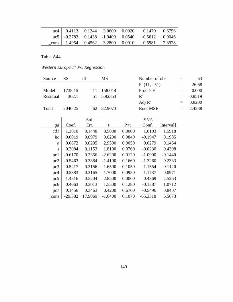
149
pc4 0.4113 0.1344 3.0600 0.0020 0.1470 0.6756 pc5 -0.2783 0.1438 -1.9400 0.0540 -0.5612 0.0046
_cons 1.4954 0.4562 3.2800 0.0010 0.5981 2.3928
Table A44.
Western Europe 1st PC Regression
Source SS df MS Number of obs = 63
F (11, 51) = 26.68
Model 1738.15 11 158.014 Prob > F = 0.000
Residual 302.1 51 5.92353 R2 = 0.8519
Adj R2 = 0.8200
Total 2040.25 62 32.9073 Root MSE = 2.4338
gd Coef.
Std.
Err. t P>t
[95%
Conf. Interval] cd1 1.3010 0.1448 8.9800 0.0000 1.0103 1.5918 hc 0.0019 0.0979 0.0200 0.9840 -0.1947 0.1985 o 0.0872 0.0295 2.9500 0.0050 0.0279 0.1464 s 0.2084 0.1153 1.8100 0.0760 -0.0230 0.4398
pc1 -0.6170 0.2356 -2.6200 0.0120 -1.0900 -0.1440 pc2 -0.5463 0.3884 -1.4100 0.1660 -1.3260 0.2333 pc3 -0.5217 0.3156 -1.6500 0.1050 -1.1554 0.1120 pc4 -0.5383 0.3165 -1.7000 0.0950 -1.1737 0.0971 pc5 1.4816 0.5204 2.8500 0.0060 0.4369 2.5263 pc6 0.4663 0.3013 1.5500 0.1280 -0.1387 1.0712 pc7 0.1456 0.3463 0.4200 0.6760 -0.5496 0.8407
_cons -29.382 17.9069 -1.6400 0.1070 -65.3318 6.5673
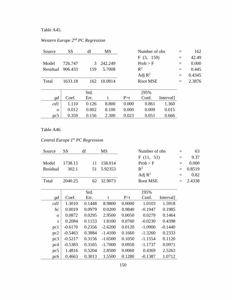
150
Table A45.
Western Europe 2nd PC Regression
Source SS df MS Number of obs = 162
F (3, 159) = 42.49
Model 726.747 3 242.249 Prob > F = 0.000
Residual 906.433 159 5.7008 R2 = 0.445
Adj R2 = 0.4345
Total 1633.18 162 10.0814 Root MSE = 2.3876
gd Coef.
Std.
Err. t P>t
[95%
Conf. Interval] cd1 1.110 0.126 8.800 0.000 0.861 1.360
o 0.012 0.002 8.100 0.000 0.009 0.015 pc5 0.359 0.156 2.300 0.023 0.051 0.666
Table A46.
Central Europe 1st PC Regression
Source SS df MS Number of obs = 63
F (11, 51) = 9.37
Model 1738.15 11 158.014 Prob > F = 0.000
Residual 302.1 51 5.92353 R2 = 0.8519
Adj R2 = 0.82
Total 2040.25 62 32.9073 Root MSE = 2.4338
gd Coef.
Std.
Err. t P>t
[95%
Conf. Interval] cd1 1.3010 0.1448 8.9800 0.0000 1.0103 1.5918 hc 0.0019 0.0979 0.0200 0.9840 -0.1947 0.1985 o 0.0872 0.0295 2.9500 0.0050 0.0279 0.1464 s 0.2084 0.1153 1.8100 0.0760 -0.0230 0.4398
pc1 -0.6170 0.2356 -2.6200 0.0120 -1.0900 -0.1440 pc2 -0.5463 0.3884 -1.4100 0.1660 -1.3260 0.2333 pc3 -0.5217 0.3156 -1.6500 0.1050 -1.1554 0.1120 pc4 -0.5383 0.3165 -1.7000 0.0950 -1.1737 0.0971 pc5 1.4816 0.5204 2.8500 0.0060 0.4369 2.5263 pc6 0.4663 0.3013 1.5500 0.1280 -0.1387 1.0712
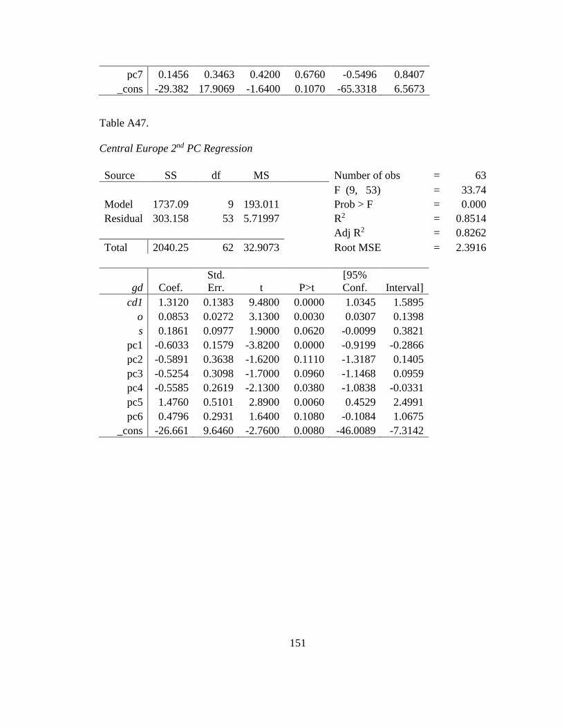
151
pc7 0.1456 0.3463 0.4200 0.6760 -0.5496 0.8407 _cons -29.382 17.9069 -1.6400 0.1070 -65.3318 6.5673
Table A47.
Central Europe 2nd PC Regression
Source SS df MS Number of obs = 63
F (9, 53) = 33.74
Model 1737.09 9 193.011 Prob > F = 0.000
Residual 303.158 53 5.71997 R2 = 0.8514
Adj R2 = 0.8262
Total 2040.25 62 32.9073 Root MSE = 2.3916
gd Coef.
Std.
Err. t P>t
[95%
Conf. Interval] cd1 1.3120 0.1383 9.4800 0.0000 1.0345 1.5895
o 0.0853 0.0272 3.1300 0.0030 0.0307 0.1398 s 0.1861 0.0977 1.9000 0.0620 -0.0099 0.3821
pc1 -0.6033 0.1579 -3.8200 0.0000 -0.9199 -0.2866 pc2 -0.5891 0.3638 -1.6200 0.1110 -1.3187 0.1405 pc3 -0.5254 0.3098 -1.7000 0.0960 -1.1468 0.0959 pc4 -0.5585 0.2619 -2.1300 0.0380 -1.0838 -0.0331 pc5 1.4760 0.5101 2.8900 0.0060 0.4529 2.4991 pc6 0.4796 0.2931 1.6400 0.1080 -0.1084 1.0675
_cons -26.661 9.6460 -2.7600 0.0080 -46.0089 -7.3142
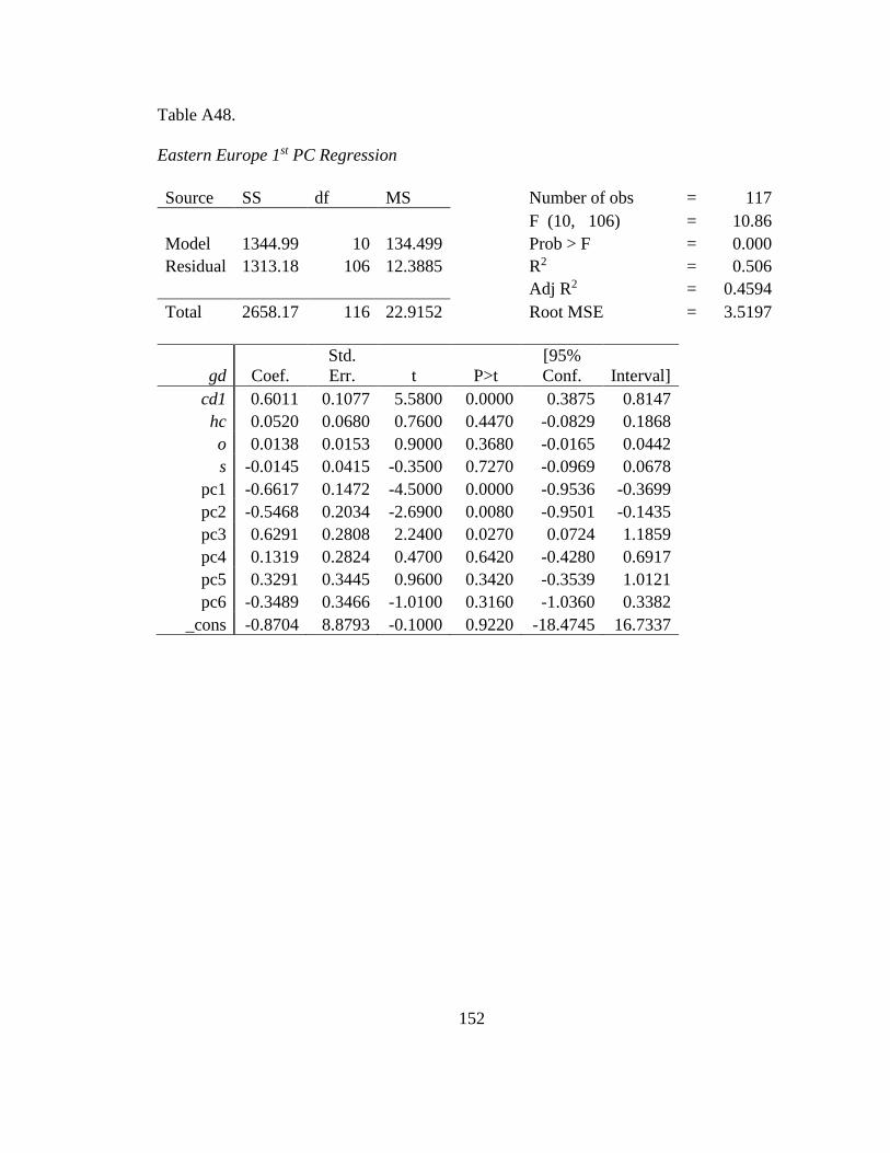
152
Table A48.
Eastern Europe 1st PC Regression
Source SS df MS Number of obs = 117
F (10, 106) = 10.86
Model 1344.99 10 134.499 Prob > F = 0.000
Residual 1313.18 106 12.3885 R2 = 0.506
Adj R2 = 0.4594
Total 2658.17 116 22.9152 Root MSE = 3.5197
gd Coef.
Std.
Err. t P>t
[95%
Conf. Interval] cd1 0.6011 0.1077 5.5800 0.0000 0.3875 0.8147 hc 0.0520 0.0680 0.7600 0.4470 -0.0829 0.1868 o 0.0138 0.0153 0.9000 0.3680 -0.0165 0.0442 s -0.0145 0.0415 -0.3500 0.7270 -0.0969 0.0678
pc1 -0.6617 0.1472 -4.5000 0.0000 -0.9536 -0.3699 pc2 -0.5468 0.2034 -2.6900 0.0080 -0.9501 -0.1435 pc3 0.6291 0.2808 2.2400 0.0270 0.0724 1.1859 pc4 0.1319 0.2824 0.4700 0.6420 -0.4280 0.6917 pc5 0.3291 0.3445 0.9600 0.3420 -0.3539 1.0121 pc6 -0.3489 0.3466 -1.0100 0.3160 -1.0360 0.3382
_cons -0.8704 8.8793 -0.1000 0.9220 -18.4745 16.7337
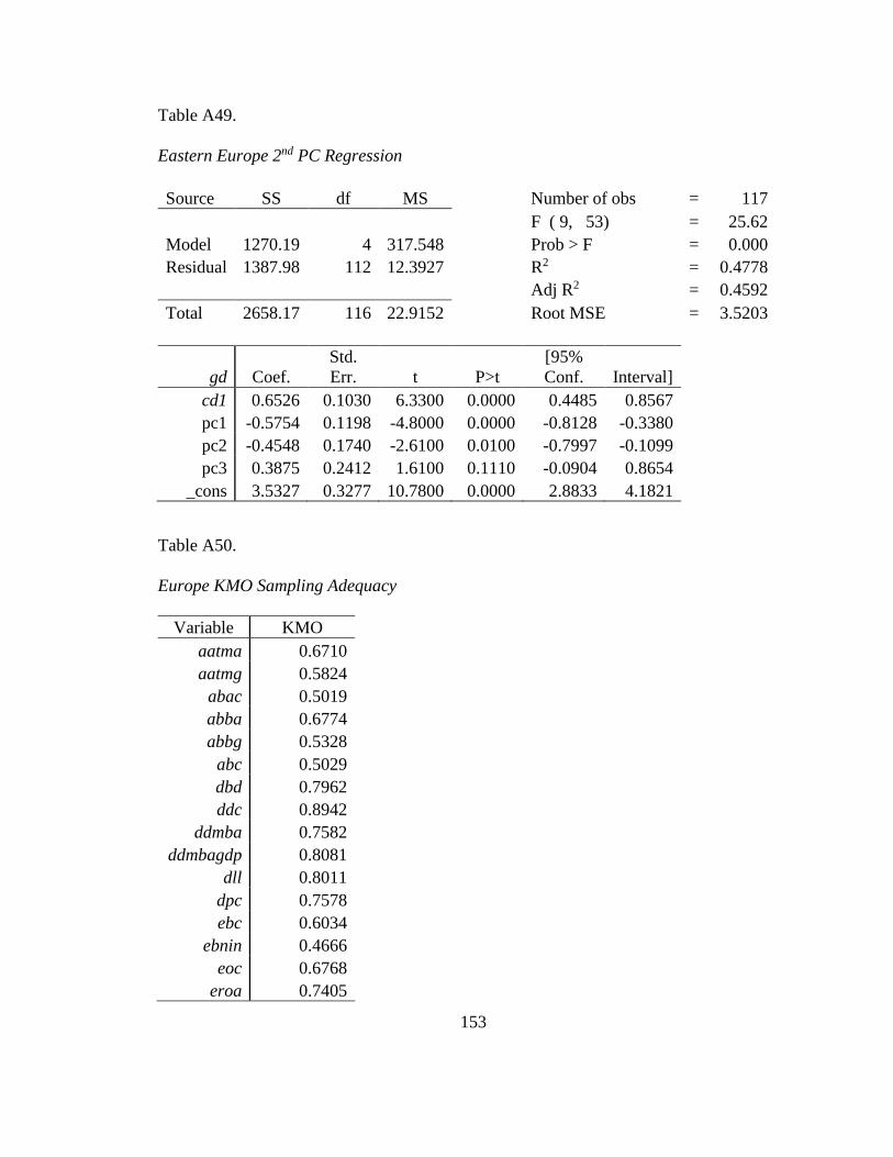
153
Table A49.
Eastern Europe 2nd PC Regression
Source SS df MS Number of obs = 117
F ( 9, 53) = 25.62
Model 1270.19 4 317.548 Prob > F = 0.000
Residual 1387.98 112 12.3927 R2 = 0.4778
Adj R2 = 0.4592
Total 2658.17 116 22.9152 Root MSE = 3.5203
gd Coef.
Std.
Err. t P>t
[95%
Conf. Interval] cd1 0.6526 0.1030 6.3300 0.0000 0.4485 0.8567 pc1 -0.5754 0.1198 -4.8000 0.0000 -0.8128 -0.3380 pc2 -0.4548 0.1740 -2.6100 0.0100 -0.7997 -0.1099 pc3 0.3875 0.2412 1.6100 0.1110 -0.0904 0.8654
_cons 3.5327 0.3277 10.7800 0.0000 2.8833 4.1821
Table A50.
Europe KMO Sampling Adequacy
Variable KMO
aatma 0.6710
aatmg 0.5824
abac 0.5019
abba 0.6774
abbg 0.5328
abc 0.5029
dbd 0.7962
ddc 0.8942
ddmba 0.7582
ddmbagdp 0.8081
dll 0.8011
dpc 0.7578
ebc 0.6034
ebnin 0.4666
eoc 0.6768
eroa 0.7405
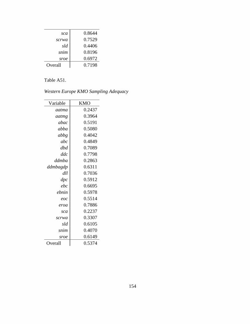
154
sca 0.8644
scrwa 0.7529
sld 0.4406
snim 0.8196
sroe 0.6972
Overall 0.7198
Table A51.
Western Europe KMO Sampling Adequacy
Variable KMO
aatma 0.2437
aatmg 0.3964
abac 0.5191
abba 0.5080
abbg 0.4042
abc 0.4849
dbd 0.7089
ddc 0.7798
ddmba 0.2863
ddmbagdp 0.6311
dll 0.7036
dpc 0.5912
ebc 0.6695
ebnin 0.5978
eoc 0.5514
eroa 0.7886
sca 0.2237
scrwa 0.3307
sld 0.6105
snim 0.4070
sroe 0.6149
Overall 0.5374

155
Table A52.
Central Europe KMO Sampling Adequacy
Variable KMO
aatma 0.7889
aatmg 0.5741
abac 0.4684
abba 0.4039
abbg 0.6010
abc 0.7850
dbd 0.6842
ddc 0.7195
ddmba 0.1807
ddmbagdp 0.5990
dll 0.6641
dpc 0.6517
ebc 0.5467
ebnin 0.4945
eoc 0.4960
eroa 0.3824
sca 0.6449
scrwa 0.7644
sld 0.7602
snim 0.4456
sroe 0.1810
Overall 0.5956
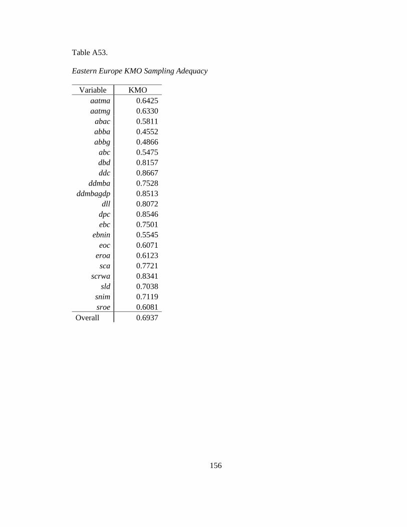
156
Table A53.
Eastern Europe KMO Sampling Adequacy
Variable KMO
aatma 0.6425
aatmg 0.6330
abac 0.5811
abba 0.4552
abbg 0.4866
abc 0.5475
dbd 0.8157
ddc 0.8667
ddmba 0.7528
ddmbagdp 0.8513
dll 0.8072
dpc 0.8546
ebc 0.7501
ebnin 0.5545
eoc 0.6071
eroa 0.6123
sca 0.7721
scrwa 0.8341
sld 0.7038
snim 0.7119
sroe 0.6081
Overall 0.6937

157
BIBLIOGRAPHY
PRIMARY SOURCES
Acemoglu, Daron, and James A. Robinson. 2006. "Economic Backwardness in Political
Perspective." American Political Science Review 100 (1): 115-131.
Allen, Franklin. 1993. "Stock markets and resource allocation." Capital Markets and
Financial Intermediation: 81-108.
Allen, Franklin, and Douglas Gale. 2000. Comparing Financial Systems. MIT Press,
Cambridge, MA.
Allen, Franklin, and Anthony M. Santomero. 1997. “The theory of financial
intermediation.” Journal of Banking & Finance 2 (11): 1461-1485
Apergis, Nicholas, Ioannis Filippidis, and Claire Economidou. 2007. "Financial
deepening and economic growth linkages: a panel data analysis." Review of World
Economics 143 (1): 179-198.
Arestis, Philip, and Panicos Demetriades. 1997. "Financial development and economic
growth: Assessing the evidence." The Economic Journal 107 (442): 783-799.
Bagehot, Walter. 1873. Lombard Street: A Description of the Money Market. Scribner,
Armstrong & Company.
Barro, Robert J., and Xavier Sala-i-Martin. 2004. Economic Growth. MIT Press,
Cambridge, MA.
Bee, Elizabeth. 2017. Contribution of maps.
Bencivenga, Valerie R., and Bruce D. Smith. 1991. “Financial intermediation and
endogenous growth.” Review of Economics Studies 58 (2): 195–209.

158
Benhabib, Jess and Mark Spiegel. 1994. “The role of human capital in economic
development; Evidence from aggregate cross-country data.” Journal of Monetary
Economics 34 (2): 143-173.
Benhabib, Jess, and Mark Spiegel. 2000. “The Role of Financial Development in Growth
and Investment.” Journal of Economic Theory 67 (4): 153-177.
Bertrand, Marianne, Antoinette Schoar, and David Thesmar. 2007. "Banking
deregulation and industry structure: Evidence from the French banking reforms of
1985." The Journal of Finance 62 (2): 597-628.
Boyd, John H., and Edward C. Prescott. 1986. "Financial intermediary-coalitions."
Journal of Economic Theory 38 (2): 211-232.
Cameron, Rondo E., Olga Crisp, Hugh T. Patrick, and Richard Tilly. 1967. Banking in
the early stages of industrialization: a study in comparative economic history.
New York: Oxford University Press.
Cattell, Raymond. B. 1966. “The scree test for the number of factors.” Multivariate
Behavioral Research 1 (2): 629-637.
Chirot, Daniel. 1989. The Origins of Backwardness in Eastern Europe: Economics and
Politics from the Middle Ages until the Early Twentieth Century. University of
California Press-Berkeley.
Christopoulos, Dimitris K., and Efthymios G. Tsionas. 2004. "Financial development and
economic growth: evidence from panel unit root and co-integration tests." Journal
of Development Economics 73 (1): 55-74.

159
Choong, Chee-Keong. 2012. "Does domestic financial development enhance the linkages
between foreign direct investment and economic growth?" Empirical
Economics 42 (3): 819-834.
Cihak, Martin., Asli Demirguc-Kunt, Erik Feyen, and Ross Levine. 2012.
“Benchmarking Financial Systems around the World.” World Bank Policy
Research Paper, 6175.
Cihak, Martin & Asli Demirguc-Kunt, Erik Feyen & Ross Levine. 2013. "Financial
Development in 205 Economies, 1960 to 2010." Journal of Financial
Perspectives, EY Global FS Institute 1 (2): 17-36.
Costello, Anna B. & Jason W. Osborne. 2005. “Best practices in exploratory factor
analysis: four recommendations for getting the most from your analysis.” Pan
Pacific Management Review 12 (2): 131-146.
Cole, David C. 1989. Reform of Financial Systems. Harvard Univ., Harvard Inst. for
International Development.
Cull, Robert, and Lixin Colin Xu. 2005. "Institutions, ownership, and finance: the
determinants of profit reinvestment among Chinese firms." Journal of Financial
Economics 77 (1): 117-146.
Davis, Lance. 1966. The capital markets and industrial concerns: The U.S. and the U.K.,
a comparative study, Economic History Review 19 (2): 255-272.
De Boyer des Roches, Jérôme. 2013. "Bank liquidity risk: From John Law (1705) to
Walter Bagehot (1873)." The European Journal of the History of Economic
Thought 20 (4): 547-57.

160
Demetriades, Panicos O., and Khaled A. Hussein. 1996. “Does financial development
cause economic growth? Time-series evidence from 16 countries.” Journal of
Development Economics 51 (2): 387-411.
Demirguc-Kunt, Asli and Ross Levine. 2001. Financial Structure and Economic Growth:
A Cross-Country Comparison of Banks, Markets, and Development. MIT Press.
Doornik, Jurgen A., and Henrik Hansen. 2008. “An omnibus test for univariate and
Multivariate normality.” Oxford Bulletin of Economics and Statistics 70: 927–
939.
Dunteman, George H. 1989. Principal Component Analysis. No. 69 Sage Publications,
Inc. Newbury Park, California.
Easterly, William, and Sergio Rebelo. 1993. “Fiscal policy and economic growth. An
empirical investigation.” Journal of Monetary Economics 32 (3):417–458.
Easterly, William, and Ross Levine. 2001. “What we have learned from a decade of
empirical research on growth? It’s not factor accumulation: stylized facts and
growth models.” World Bank Economic Review 15 (2): 177-219.
Finch, Holmes. 2006. "Comparison of the performance of varimax and promax rotations:
Factor structure recovery for dichotomous items." Journal of Educational
Measurement 43 (1): 39-52.
Fisher, Irving. 1933. "The debt-deflation theory of great depressions," Econometrica 1
(4): 337-357.
FitzGerald, Valpy. 2007. "Financial development and economic growth: a critical view.
Flat World, Big Gaps, ed. Kwame Sundaram Hyderadad: Orient Longman.”

161
Frankel, Jeffrey, and David Romer. 1999. “Does trade cause growth?” American
Economic Review 89 (3): 379–399.
Freeman, John. 1986. "Entrepreneurs as organizational products: Semiconductor firms
and venture capital firms." Advances in the study of entrepreneurship, innovation,
and economic growth 1: 33-52.
Gerschenkron, Alexander. 1952. “Economic Backwardness in Historical Perspective.” In
The Progress of Underdeveloped Areas, edited by Bert F. Hoselitz. Chicago:
University of Chicago Press.
Goldsmith, Raymond. W. 1968. Financial Structure and Development, New Haven, CT:
Yale University Press.
Granger, Clive W. J., and Paul Newbold. 1974. "Spurious regressions in econometrics."
Journal of Econometrics 2 (2): 111–120.
Green, Roy. 1989. "Real bills doctrine." In Money, pp. 310-313. Palgrave Macmillan
UK.
Greenwood, Jeremy, and Boyan Jovanovic. 1990. “Financial development, growth, and
the distribution of income.” Journal of Political Economy 98:1076–1107.
Greenwood, Jeremy and Bruce D. Smith. 1996. "Financial markets in development, and
the development of financial markets.” Journal of Economic Dynamics and
Control 21 (1):145-181.
Griese, Thomas, Manfred Kraft, & Daniel Meierrieks, 2009. “Linkages between financial
deepening, trade openness and economic development: causality evidence from
Sub-Saharan Africa.” World Development 37 (12): 1849-1860.

162
Grossman, Gene M., and Elhanan Helpman. 1991."Trade, knowledge spillovers, and
growth." European Economic Review 35 (2-3): 517-526.
Guiso, Luigi, Paola Sapienza, and Luigi Zingales. 2004. “The role of social capital in
financial development.” The American Economic Review 94 (3): 526-556.
Gurley, John G., and Edward S. Shaw. 1955. "Financial aspects of economic
development." The American Economic Review 45 (4): 515-538.
Haber, Stephen H. 1991. "Industrial concentration and the capital markets: A
comparative study of Brazil, Mexico, and the United States, 1830–1930." The
Journal of Economic History 51 (03): 559-580.
Hauner, David. 2009. “Public debt and financial development.” Journal of
Development Economics 88 (1): 171-183.
Hotelling, Harold. 1933. “Analysis of a complex of statistical variables into principal
components.” Journal of Education Psychology 24 (6): 417–441.
Hotelling, Harold. 1936. “Simplified calculation of principal components.”
Psychometrika 1 (1): 27–35.
Humphrey, Thomas M. 1982. "The real bills doctrine." Federal Reserve Bank of
Richmond.
Jolliffe, Ian T. 1982. "A note on the use of principal components in regression." Journal
of Applied Statistics 31 (3): 300-303.
Kaiser, Henry F. 1958. ‘The Varimax criterion for analytic rotation in factor analysis’,
Psychometrika 23: 187.
163
Kaiser, Henry F. 1960. “The application of electronic computers to factor analysis.”
Educational Psychological Measurement 20: 141-151.
Katchova, Ani. 2013. Principal Component analysis and Factor Analysis. Econometric
Academy website:sites.google.com/site/economietric academy.
https://youtu.be/hnzW8UxQlvo.
Khan, Mr Mohsin S., and Mr A. Senhadji Semlali. 2000. “Financial development and
economic growth: an overview.” No. 0-209. International Monetary Fund.
King, Robert and Ross Levine. 1993. Finance and growth: Schumpeter might be right.”
The Quarterly Journal of Economics 108 (3): 717-737.
LaPorta, Rafael, Florencio Lopez-de-Silanes, Andrei Shleifer, and Robert Vishny. 2000.
“Investor protection and corporate governance.” Journal of Financial Economics
58 (1): 3-27.
Lavrenko, Victor and Sean Moran. 2015. "Graph regularized hashing." In European
Conference on Information Retrieval, pp. 135-146. Springer International
Publishing.
Law, John. 1966. Money and trade considered. AM Kelley.
Levine, Ross. 1997. “Financial development and economic growth: views and agenda.”
Journal of Economic Literature 35 (2): 688-726.
Levine, Ross. 1999. "Law, finance, and economic growth." Journal of Financial
Intermediation 8 (1): 8-35.
Levine, Ross. 2002. "Bank-based or market-based financial systems: which is better?"
Journal of Financial Intermediation 11 (4): 398-428.

164
Levine, Ross. 2005. “Finance and growth: theory and evidence.” Handbook of Economic
Growth 1: 865-934.
Levine, Ross, Norman Loayza, and Thorsten Beck. 2000. "Financial intermediation and
growth: causality and causes." Journal of Monetary Economics 46 (1): 31-77.
Levine, Ross, and Sara Zervos. 1998. "Stock markets, banks, and economic
growth." American Economic Review: 537-558.
Lipovina-Bozovic, Milena, and Julija Cerovic Smolovic. 2016. "Evidence on Economic
Growth and Financial Development in Montenegro." Management 11 (4): 349-
365.
Loayza, Norman, and Romain Ranciere. 2002. "Financial fragility, financial
development, and growth." World Bank mimeo 88.
Lucas, Robert E. 1988. “On the mechanics of economic development,” Journal of
Monetary Economics 22 (1): 3-42.
Lucas, Robert. E. 1993. “Making a miracle.” Econometrica 61 (2): 251–272.
McKinnon, Ronald. I. 1973. “Money and capital in economic development.” Washington,
DC: Brookings Institution.
Merton, Robert C., and Zvi Bodie. 1995. "A conceptual framework for analyzing the
financial system." The Global Financial System: A Functional Perspective: 3-31
Naghshpour, Shahdad. 2013. Fundamentals of Money and Financial Systems. Business
Expert Press.
Neusser, Klaus, and Maurice Kugler. 1998. "Manufacturing growth and financial
development: evidence from OECD countries." Review of Economics and

165
Statistics 80 (4): 638-646.
Pagano, Marco. 1993. “Financial markets and growth: an overview.” European Economic
Review 37 (2): 613–622.
Patrick, Hugh T. 1966. “Financial development and economic growth in underdeveloped
countries.” Economic Development and Cultural Change 14 (2): 174-189.
Pearson, Karl. 1901. “On lines and planes of closest fit to systems of points in space.”
The London, Edinburgh, and Dublin Philosophical Magazine and Journal of
Science 2 (11): 559–572.
Rebelo, Sergio T. 1991. “Long-Run Policy Analysis and Long-Run Growth.” Journal
of Political Economy, 99 (3): 500-521.
Rioja, Felix, and Neven Valev. 2004. “Does one size fit all? A reexamination of the
finance and growth relationship.” Journal of Development Economics 74 (2):
429-447.
Robinson, Joan. 1952. "The Generalization of the General Theory”, In: the Rate of
Interest and Other Essays, London: MacMillan.
Romer, Paul M. 1986. “Increasing Returns and Long-Run Growth,” Journal of Political
Economy 94: 1002–1037.
Romer, Paul. 1990. “Endogenous technological change.” Journal of Political Economy
98 (5): 71–102.
Rostow, Walt. W. 1956. “The take-off into self-sustained growth.” The Economic
Journal 66 (261): 25-48.
166
Rostow, Walt. W. 1960. The Stages of Economic Growth: A Non-Communist Manifesto.
Cambridge University Press.
Schumpeter, Joseph. 1911. The Theory of Economic Development: An Inquiry into
Profits, Capital, Credit, Interest and Business Cycle. Cambridge, Mass: Harvard
University Press.
Shaw, Edward S. 1973. Financial Deepening in Economic Development. Oxford
University Press, London and New York.
Shlens, Jonathon. 2014. “A tutorial on principal component analysis.” arXiv preprint
arXiv:1404.1100.
Solow, Robert M. 1956. "A contribution to the theory of economic growth." The
Quarterly Journal of Economics 70 (1): 65-94.
Tadesse, Solomon. 2002. "Financial architecture and economic performance:
international evidence." Journal of Financial Intermediation 11 (4): 429-454.
Williams, Brett, Andrys Onsman, and Ted Brown. 2010. "Exploratory factor analysis: A
five-step guide for novices." Australasian Journal of Paramedicine 8 (3).
Wooldridge, Jeffrey M. 2010. Introductory Econometrics: A Modern Approach. Mason,
OH: Southwestern Cengage Learning.
World Bank. 2004. International Bank for Reconstruction and Development / World
Bank 1818 H Street NW, Washington DC 20433.
World Bank. 2012. International Bank for Reconstruction and Development / World
Bank 1818 H Street NW, Washington DC 20433.
World Bank. 2015. World Development Indicators. Washington, DC: World Bank

167
Group. Online at data.worldbank.org/data-catalog/world-development
indicators/.
Xu, Zhenhui. 2000. “Financial Development, investment, and economic growth.”
Economic Inquiry 38 (2): 331-344.
SECONDARY SOURCES
Abbas, SM Ali, and Jakob Christensen. 2007. "The Role of Domestic Debt Markets in
Economic Growth: An Empirical Investigation for Low-Income Countries and
Emerging Markets." IMF Working Papers: 1 – 40. Available at SSRN:
hhtps://.com/abstract=995628.
Abramovitz, Moses. 1986. "Catching Up, Forging Ahead, and Falling Behind." The
Journal of Economic History 46 (2): 385-406.
Adu, George, George Marbuah, and Justice Tei Mensah. 2013. "Financial development
and economic growth in Ghana: Does the measure of financial development
matter?" Review of Development Finance 3 (4): 192-203.
Aghion, Phillipe and Peter Howitt. 1998. Endogenous Growth Theory. MIT Press,
Cambridge, MA.
Aghion Phillipe, Peter Howitt, and David Mayer-Foulkes. 2005. “The effect of financial
development on convergence theory and evidence.” Quarterly Journal of
Economics 120, 173–222.
Amable, Bruno. 1993. “Catch-up and Convergence in a Model of Cumulative Growth.”
International Review of Applied Economics 7 (1): 1-25.
Ang, James B., and Warwick J. McKibbin. 2007. "Financial Liberalization, Financial
168
Sector Development and Growth: Evidence from Malaysia." Journal of
Development Economics 84 (1): 215-233.
Arcand, Jean-Louis, Enrico Berkes, and Ugo Panizza. 2012. “Too Much Finance?
International Monetary Fund.” IMF Working Papers 161.
Asongu, Simplice A. 2015. "Financial sector competition and knowledge economy:
Evidence from SSA and MENA countries." Journal of the Knowledge Economy
6 (4): 717-748.
Atiq, Zeeshan and Emanul Haque. 2014. “Financial Development and Economic
Growth: The Role of Financial Liberalization.” Available at SSRN 2407358.
Ball, V. Eldon, Charles Hallahan, and Richard Nehring. 2004. "Convergence of
productivity: an analysis of the catch-up hypothesis within a panel of states."
American Journal of Agricultural Economics 86 (5): 1315-1321.
Bangake, Chrysost, and Jude C. Eggoh. 2011. "Further evidence on finance-growth
causality: A Panel Data Analysis." Economic Systems 35 (2): 176-188.
Banko, Zoltan, Laszlo Dobos, Janos Abonyi. 2011. Dynamic Principal Component
analysis in Multivariate Time-Series Segmentation. Conservation, Information,
Evolution-towards a sustainable engineering and economy 1 (1): 11-24.
Barnett, William II. 2007. "Dimensions and Economics: Some Problems." Quarterly
Journal of Austrian Economics 7 (1): 95-104.
Barro, Robert J. 1997. Determinants of Economic Growth: A Cross Country Empirical
Study. MIT Press, Cambridge, MA.
Barro, Robert J., and Xavier Sala-i-Martin. 1995. Economic Growth. Boston, Mass.:

169
McGraw Hill.
Baum, Christopher. 2006. An Introduction to Modern Econometrics Using Stata. College
Station, TX: Stata Press.
Bhattacharjee, Sudarshan, and Hariprasad Chic Govinda. 2015. "Commercial Banks’
Performance in India during Sub-Prime Meltdown." Asian Journal of Research in
Banking and Finance 5 (6): 75-84.
Bideleux, Robert and Ian Jeffries. 1998. A History of Eastern Europe: Crisis and
Change. Psychology Press.
Bittencourt, Manoel. 2012. “Financial Development and Economic Growth in Latin
America: Is Schumpeter Right?” Journal of Policy Modeling 34 (3): 341-355.
Brenner, Robert. 1989. “Economic backwardness in Eastern Europe in Light of
Development in the West.” The origins of backwardness in Eastern Europe:
Economics and politics from the middle ages until the early twentieth century:
15-52.
Bryant, Fred B., and Paul R. Yarnold. 1995. "Principal-components analysis and
exploratory and confirmatory factor analysis." In: Grimm & Yarnold, (Eds.),
Reading and Understanding Multivariate Statistics, fourth ed. American
Psychological Association, Washington: 99–136.
Calderón, César, and Lin Liu. 2003. "The direction of causality between financial
development and economic growth." Journal of Development Economics 72 (1):
321-334.
Choi, In and Bhum Suk Chung. 1995. “Sampling frequency and the power of tests for a
170
unit root: A simulation study.” Economics Letters 49 (2): 131-136.
Darrat, Ali F. 1999. “Are financial deepening and economic growth causally related?
Another look at the evidence.” International Economic Journal 13 (3): 19-35.
Dawson, P. J. 2003. "Financial development and growth in economies in transition."
Applied Economics Letters 10 (13): 833-836.
De Gregorio, Jose, and Pablo E. Guidotti. 1995. “Financial development and economic
growth.” World Development 23 (3): 433-448.
Demetriades, Panicos O., and Kul B. Luintel. 1996. "Financial development, economic
growth and banking sector controls: evidence from India." The Economic
Journal: 359-374.
Diaz, Pantoja Augusto, Roberto Carlos Lanuza and Clyde Xaviera Delgadillo. 2013.
“Financial development, trade openness and growth: A causality analysis for the
Central American countries.” Banco Central de Nicaragua.
Draper, Norman, and Harry Smith. 2014. Applied Regression Analysis. Wiley & Sons.
Gaffeo, Edoardo, and Petya Garalova. 2014. "On the finance-growth nexus: additional
evidence from Central and Eastern Europe countries." Economic Change and
Restructuring 47 (2): 89-115.
Graff, Michael. 2002. “Causal Links between Financial Activity and Economic Growth:
Empirical Evidence from a Cross-Country Analysis, 1970-1990.” Bulletin of
Economics Research 54 (2):119-133.
Graff, Michael. 2005. “Socio-economic factors and the finance-growth nexus.” The
European Journal of Finance 11 (3):183-205.
171
Gregor, Paul. 1974. “A note on relative backwardness and industrial structure.” The
Quarterly Journal of Economics 74 (8): 520-527.
Gurley, John G. and Edward S. Shaw. 1967. “Financial structure and economic
development.” Economic Development and Cultural Change 15 (3): 257-268.
Hadi, Ali S. and Robert F. Ling. 1998. “Some Cautionary Notes on the Use of Principal
Component Regression.” The American Statistician 52 (1): 15–19.
Hassan, M.Kabir, Benito Sanchez, and Jung-SukYu. 2011. “Financial development and
economic growth: new evidence from panel data.” The Quarterly Review of
Economics and Finance 51 (1): 88-104.
Heckman, James. J. 2008. “Econometric causality.” International Statistical Review 76
(1): 1-27.
Hicks, John R. 1969. A Theory of Economic History. Vol 163. Oxford: Oxford University
Press.
Hondroyiannis, George, Sarantis Lolos, and Evangelia Papapetrou. 2005. "Financial
markets and economic growth in Greece, 1986–1999." Journal of International
Financial Markets, Institutions and Money 15 (2):173-188.
Huang, Yongfu, and Jonathan Temple. 2005. “Does external trade promote financial
development?” Discussion Paper No. 5150. London: Centre for Economic Policy
Research.
Huang, Yongfu. 2010. Determinants of Financial Development. London. Palgrave
McMillan.
Hue, Qazi Muhammad, and Faridul Islam. 2013. “Does financial development hamper
172
economic growth: empirical evidence from Bangladesh?” Journal of Business
Economics and Management 14 (3): 558-582.
Jalil, Abdul, and Mete Feridun. 2011. “Impact of financial development on economic
growth: empirical evidence from Pakistan.” Journal of Asia Pacific Economy 16
(1): 71-80.
Jolliffe, Ian T. 1989. "Rotation of ill-defined principal components." Applied Statistics 38
(1): 139-147.
Jolliffe, Ian. T. 2002. Principal Component Analysis. Springer Series in Statistics. New
York. 2nd Ed.
Jung, Woo S. 1986. "Financial development and economic growth: international
evidence." Economic Development and Cultural Change 34 (2): 333-346.
Kaiser, Henry F. 1974. “An index of factor simplicity.” Psychometrika 39: 31–36.
Kenza, Medjahed, and Benbouziane Mohamed. 2015. “Financial development and
economic growth in Algeria: An econometric analysis of the transmission
channels.” International Journal of Economic and Business Review 3 (2): 5-14.
Kiyotaki, Nobuhiro and John Moore. 2005. Liquidity and asset prices. International
Economic Review 46 (2): 317-349.
Ledesma, Rubén Daniel, and Pedro Valero-Mora. 2007. "Determining the number of
factors to retain in EFA: An easy-to-use computer program for carrying out
parallel analysis." Practical assessment, research & evaluation 12 (2): 1-11.
Leech, Nancy L, Karen Caplovitz Barrett, and George Arthur Morgan. 2005. SPSS for
Intermediate Statistics. Use and Interpretation. 2nd edition, Lawrence Erlbaum

173
Associates Inc. New Jersey.
Luintel, Kul B., and Mosahid Khan. 1999. "A quantitative reassessment of the finance
growth nexus: Evidence from a multivariate VAR." Journal of Development
Economics 60 (2): 381-405.
Mbate, Michael. 2013. “Domestic debt, private sector credit and economic growth in
Sub-Saharan Africa.” African Development Review 25 (4): 434-446.
Mhadhbi, Khalil. 2014. "Financial development and economic growth: A dynamic panel
data analysis." International Journal of Econometrics and Financial Management
2 (2): 48-58.
Mitchell, Tanisha. 2015. "Bank default prediction: A comparative model using principal
component analysis." Journal of Stock & Forex Trading 4 (149): 2.
Moore, Basil J. 1975. “Financial Deepening in Economic Development.” by Edward S.
Shaw Review by: Basil J. Moore Journal of Money, Credit and Banking 7 (1):
124-130.
Murthy, KV Bhanu. 2015. "Examining the relationship between financial development
and economic development." MUDRA: Journal of Finance and Accounting, 1
(1).
Myant, Martin and Jan Drahokoupil. 2011. Transition Economies: Political Economy in
Russia, Eastern Europe, and Central Asia. Hoboken, New Jersey: Wiley.
Nain, Md Zulquar, and Bandi Kamaiah. 2014. "Financial development and economic
growth in India: Some evidence from non-linear causality analysis." Economic
Change and Restructuring 47 (4): 299-319.

174
Nason, Guy P. 2006. "Stationary and non-stationary times series." Statistics in
Volcanology. Special Publications of IAVCEI 1 000-000.
Olawale, Fatoki, and David Garwe. 2010. “Obstacles to the growth of new SMES in
South Africa: A principal component analysis approach.” African Journal of
Business Management 4 (5): 729-738.
Parinet, Bernard, Antoine Lhote, and Bernard Legube. 2004. "Principal component
analysis: an appropriate tool for water quality evaluation and management
application to a tropical lake system." Ecological Modelling 178 (3): 295-311.
Penn State University. 2016. Lesson 11: Principal Component Analysis (PCA) Stat 505.
https://onlinecourses.science.psu.edu/stat505/node/49.
Pradhan, Rudra P., Mak B. Arvin, and John H. Hall. 2015. "Economic growth,
development of telecommunications infrastructure, and financial development in
Asia, 1991–2012." The Quarterly Review of Economics and Finance 59:25-38.
Pradhan, Rudra P., Mak B. Arvin, Sahar Bahmani, John H. Hall, and Neville R. Norman.
2017. "Finance and growth: Evidence from the ARF countries." The Quarterly
Review of Economics and Finance. February.
Ratna Sahay, Martin Cihak, Papa N’Diaye, Adolfo Barajas, Ran Bi, Diana Ayala,
Yuan Gao, Annette Kyobe, Lam Nguyen, Christian Saborowski, Katsiaryna
Svirydzenka, and Seyed Reza Yousefi. 2015. “Rethinking financial deepening:
stability and growth in emerging markets.” Revista de Economia Institucional 17
(33): 73-107.
Razali, Nornadiah; Wah, Yap Bee. 2011. "Power comparisons of Shapiro-Wilk,
175
Kolmogorov-Smirnov, Lilliefors and Anderson-Darling tests." Journal of
Statistical Modeling and Analytics 2 (1): 21–33.
Rioja, Felix, and Neven Valev. 2004. “Finance and the Sources of Growth at Various
Stages of Economic Development.” Economic Inquiry 42 (1): 127–140.
Rousseau, Peter L., and Paul Wachtel. 1998. "Financial intermediation and economic
performance: historical evidence from five industrialized countries." Journal of
Money, Credit and Banking: 657-678.
Samargandi, Nahla, Jan Fidrmuc, and Sugata Ghosh. 2014. "Financial development and
economic growth in an oil-rich economy: The case of Saudi Arabia." Economic
Modelling 43: 267-278.
Samargandi, Nahla, Jan Fidrmuc, and Sugata Ghosh. 2015. "Is the relationship between
financial development and economic growth monotonic? Evidence from a sample
of middle-income countries." World Development 68: 66-81.
Shan, Jordan, and Alan Morris. 2002. "Does financial development lead economic
growth?" International Review of Applied Economics 16 (2): 153-168.
Simoglou, Alexandros, E. B. Martin, and A. J. Morris. 2002. "Statistical performance
monitoring of dynamic multivariate processes using state space
modelling." Computers & Chemical Engineering 26 (6): 909-920.
Singha, Bulbul. 2015. "The dynamics of finance and growth: empirical evidence from
Bangladesh.” Bangladesh Research Publications Journal 10 (4): 321-329.
Stern, David I. 2011. “From correlation to granger causality.” Crawford School of
Economics and Government Research Paper 13.

176
Stiglitz, Joseph. 1992. “The design of financial systems for the newly emerging
democracies of Eastern Europe,” in C. Clague and G. Raussere (Eds.), The
Emergence of Market Economies in Eastern Europe (Oxford: Basil Blackwell).
Stoicaa, Seyed Mehdian, and Alina Sargu. 2015. “The impact of internet banking on the
performance of Romanian banks: DEA and PCA approach.” Procedia Economic
and Finance 20: 610-622.
Tang, Chor Foon, and Bee Wah Tan. 2014. "The linkages among energy consumption,
economic growth, relative price, foreign direct investment, and financial
development in Malaysia." Quality & Quantity 48 (2): 781-797.
Thompson, Bruce & Larry G. Daniel. 1996. “Factor analytic evidence for the construct
validity of scores: A historical overview and some guidelines.” Educational and
Psychological Measurement 56:197-208.
Varlık, Nimet. 2016. "The Relationship between Financial Development and Financial
Fragility in Turkey, the period of 1990-2014." Ekonomik Yaklasim 27 (98): 141-
176.
Veblen, Thorstein. 1990. Imperial Germany and Industrial Revolution. Transaction
Publishers.
Zhang, Jim., Lanfang Wang, and Susheng Wang. 2012. “Financial development and
economic growth: recent evidence from China.” Journal of Comparative
Economics 40 (3): 393-412.