Embed Size (px)
Citation preview

FEDERAL RESERVE BANK OF SAN FRANCISCO
WORKING PAPER SERIES
The Industry-Occupation Mix of U.S. Job Openings and Hires
Bart Hobijn
Federal Reserve Bank of San Francisco
VU University Amsterdam, and Tinbergen Institute
July 2012
The views in this paper are solely the responsibility of the authors and should not be
interpreted as reflecting the views of the Federal Reserve Bank of San Francisco or the
Board of Governors of the Federal Reserve System.
Working Paper 2012-09 http://www.frbsf.org/publications/economics/papers/2012/wp12-09bk.pdf
The Industry-Occupation Mix
of U.S. Job Openings and Hires
BART HOBIJN 1
Federal Reserve Bank of San Francisco,
VU University Amsterdam, and Tinbergen Institute
This Version: July 11, 2012.
Abstract
I introduce a method that combines data from the U.S. Current Population Survey, Job Openings and Labor
Turnover Survey, and state-level Job Vacancy Surveys to construct annual estimates of the number of job
openings in the U.S. in the Spring by industry and occupation. I present these estimates for 2005-2011. The
results reveal that: (i) During the Great Recession job openings for all occupations declined. (ii) Job openings
rates and vacancy yields vary a lot across occupations. (iii) Changes in the occupation mix of job openings and
hires account for the bulk of the decline in measured aggregate match efficiency since 2007. (iv) The majority of
job openings in all industries and occupations are filled with persons who previously did not work in the same
industry or occupation.
Keywords: Job openings, labor market mobility, measurement, occupations.
JEL-codes: J23, J60, J63.
1 Email: [email protected]. I am grateful to Colin Gardiner, Brian Lucking, and Ted Wiles for their outstanding research
assistance. I would like to thank Mike Elsby, Erica Groshen, Galina Hale, Oscar Jorda, Chris Nekarda, Ayşegül Şahin, and Rob
Valletta for their comments and suggestions. The views expressed in this paper solely reflect those of the author and not
necessarily those of the Federal Reserve Bank of San Francisco, nor those of the Federal Reserve System as a whole.
The Mix of U.S. Job Openings and Hires
2
1. Introduction
Labor markets are characterized by the fact that at any time there are unemployed persons who are
not working who are looking for a job and, at the same time, there are employers who have
vacancies that they have not filled yet.
There is a wealth of data on the characteristics of the pool of unemployed workers in the U.S., in
large part based on the Current Population Survey (CPS). For the unemployed we know their
demographic characteristics, how long they have been searching for a job, whether they have
previous work experience and, if so, in what industry and occupation.
Contrary to the data on the unemployed, U.S. data on job openings, or vacancies,2 are very
sparse. Whereas in many other industrialized countries potential employers register their job
openings with a particular agency, no such organization exists in the U.S. Thus, no official
administrative data on unfilled vacancies is available for the U.S.3 As a result, analyses of U.S.
labor demand have resorted to alternative data sources on vacancies.
Highly aggregated data are available from the Conference Board‟s Help-Wanted (HWI) and
Help-Wanted Online (HWOL) indices. Though these indices have proven to be helpful proxies for
U.S. labor demand, the way they are constructed is not very precise about what constitutes a job
opening and about how representative the set of newspapers and online job sites, that is used as
source data, is.4 Moreover, these indices do not provide much detail on job openings by industry
and occupation.5
Since 2001 the Bureau of Labor Statistics (BLS) publishes a survey-based estimate of the
number of job openings as part of its Job Openings and Labor Turnover (JOLTS) release that is
based on a more formal sampling method than the HWI and HWOL and on a more consistent
definition of what is a job opening.6
2 I use the terms “job opening” and “vacancy” interchangeably throughout this paper. 3 See Ferber (1966, Part II) for an early overview of vacancy data in other countries. 4 For example, because of shifts in vacancy postings in newspapers and online comparing these indices over time requires several
adjustments. Three studies that make such adjustments are Abraham (1987), Valletta (2005), and Barnichon (2010). 5 Proprietary data underlying the HWOL that contains more information on vacancies by occupation can be obtained from the
Conference Board. This is the data used by Şahin et. al. (2011), for example. 6 The formal definition applied in JOLTS can be found at http://www.bls.gov/jlt/jltdef.htm. See Clayton et. al. (2011) for a discussion
of the merits and limitations of the JOLTS data.
Bart Hobijn
3
Figure 1 compares the number of job openings from JOLTS with the number of online help-
wanted ads counted in the HWOL. As can be seen from the figure, both series show a similar
cyclical pattern in the sense that labor demand started to decline mid-2007 and dropped throughout
the recession. The HWOL index shows a much stronger rebound in vacancy postings than the
JOLTS. In fact, it suggests that the number of vacancies in the Spring of 2012 exceeded that in the
2007. The JOLTS measure implies that there were one million job openings less in 2012 than in
2007. The JOLTS data is much more in line with other labor market indicators that suggest a very
slow recovery in labor market conditions after the Great Recession.
In addition to the number of job openings, the JOLTS release contains two other pieces of data.
First, it includes data on job openings by major industry and, second, it also includes the number of
persons actually hired. The fact that JOLTS includes both data on vacancies and hires is very useful,
since it provides direct evidence on the rate with which potential employers and employees are
matched in the labor market. This measure is the number of hires per vacancy, known as the
vacancy yield (Davis, Faberman, and Haltiwanger, 2010).
Many recent studies have focused on movements in the vacancy yield after 2007. The aggregate
vacancy yield rose when the number of unemployed increased and the number of vacancies
declined. However, this increase was much smaller than implied by commonly used matching
functions, like those described in Petrongolo and Pissarides (2001). This suggests a potential
increase in labor market frictions due to a lower efficiency with which the unemployed are matched
with job openings.7
Studies that analyzed industry-level vacancy yield data from JOLTS, like Davis, Faberman and
Haltiwanger (2012) and Barnichon et. al. (2012), have found that a large part of the apparent decline
in aggregate match efficiency is due to the construction sector, which has a vacancy yield that is 2.5
times the average. A shift in the composition of job openings away from construction thus might
result in a decline in measured aggregate match efficiency even if that of each of the underlying
industries does not decline.
7 See, for example, Borowczyk-Martins et. al. (2011) or Sedláček (2011). Several studies specifically focus on the effect of the
decline in match efficiency on the rightward shift in the U.S. Beveridge curve. Among them are Barnichon, Elsby, Hobijn, and
Şahin (2012), Daly, Hobijn, Şahin, and Valletta (2012), Dickens (2009), Dickens and Triest (2012), Lubik (2011), and Sterk
(2010).

The Mix of U.S. Job Openings and Hires
4
Thus, shifts in the composition of vacancies, and of economic activity more generally, have a
big influence on the cyclical fluctuations of the vacancy yield. Because the JOLTS data do not
contain job openings and hires by occupation, it is, however, not possible to use them to figure out
whether the effect of this compositional shift is due to industries hiring workers in different
occupations or whether their overall levels of labor demand have changed. In order to answer this
question one would need data on job openings and hires by industry and occupation, which are not
available.
In this paper, I construct estimates of annual time series of job openings and hires in the U.S. by
industry and occupation covering 2005 through 2011. I do so by combining data from three
different sources. The first is JOLTS, from which I use data on job openings and hires by industry.
The second is the Current Population Survey (CPS) that I use to construct the distribution of hires
by occupation for each industry. The final source is a set of state-level Job Vacancy Surveys (JVSs),
not previously used in the analysis of the U.S. labor market, that contain data on job openings by
occupation. The states in the JVS sample cover about 10 percent of U.S. payrolls and the labor
force.
Using a very parsimonious parameterization of the number of hires per vacancy by industry and
occupation, I combine the data from these three sources to estimate the parameters using exactly
identified method of moments. Unfortunately, because of the lack of information about the
sampling weights in JOLTS and JVSs, it is not possible to calculate standard errors of the estimates.
To check the validity of the results, however, I perform what amounts to an informal test of
overidentifying restrictions using data on vacancies by major industry for a subset of states from the
JVS sample.
The result of the estimation method is a set of estimates of job openings by industry and
occupation during the second quarter of each year in my sample and the number of hires by industry
and occupation from the second quarter of each year in the sample through the first quarter in the
next year. The estimates are restricted to add up to the published data on job openings and hires by
industry from JOLTS.
Four things stand out from the results. They turn out to mainly pertain to the occupation
dimension of the data. First, the Great Recession was broad-based resulting in a decline in the
number of job openings for all occupations. Second, there is a lot of variation in job openings rates
Bart Hobijn
5
and vacancy yields across occupations. Third, the shift in the occupation mix of job openings and
hires since 2007 accounts for the bulk of the decline in measured aggregate match efficiency that
has led to the rightward movement of the Beveridge curve. A large part of this shift is due to the
different cyclical sensitivity of job postings across occupations and will likely unravel as the labor
market recovery gains steam. Finally, the majority of job openings in all industries and occupations
are filled with persons who previously did not work in the same industry or occupation.
The structure of the rest of the paper is as follows. In section 2 I introduce the methodology that
allows me to combine the three data sources to get estimates of job openings and hires by industry-
occupation combination. In section 3 I briefly discuss the data sources. I present the main results on
the industry-occupation mix of job openings and hires in section 4. In section 5 I show how
important the change in this mix has been for movements in the number of hires per vacancy. In
section 6 I provide some evidence on who is hired in the vacancies posted and discuss the
implications of these facts for our understanding of the dynamics of the U.S. labor market. I
conclude in section 7. The appendix contains details on the mathematical results used in the main
text.
2. Methodology
The aim of this paper is to construct annual time series of the number of vacancies and hires by
industry-occupation combination. All of these measures are constructed to add up to the published
industry-level JOLTS data on job openings and hires. I construct these measures by combining data
from JOLTS, the CPS, and state-level JVSs.
Throughout the analysis, I index industries by and occupations by . The
number of industries, , is 17, which is the number of 2-digit NAICS industries for which JOLTS
data are published. The number of occupations, , is 22 which is the number of 2-digit level SOC
codes for which job openings are reported in the state-level JVSs. This makes for 374 industry-
occupation combinations. I skip a time subscript. All variables defined are assumed to apply to the
same year.
For the stock of vacancies, I denote the average number of job openings in the U.S. in industry
for occupation over the three months in the second quarter of a year by . For the flow of hires, I

The Mix of U.S. Job Openings and Hires
6
write the number of hires in the U.S. in industry and occupation from the second quarter of a
year through the first quarter of the next year as . The reason that I evaluate the flow of hires
over a whole year is that I construct these flows from the CPS and that, because I am using 374
industry-occupation cells, shorter time-spans will result in relatively small samples.
My methodology involves combining data for the U.S. from JOLTS with data from state-level
job vacancy surveys. Unfortunately, not all states run such a survey. As a result, I also need to
define the stock of vacancies and flow of hires for the states that run a job vacancy survey (JVS
states). Throughout, I denote these aggregates by an asterisk, *. That is, , is the average number
of job openings in JVS states in industry for occupation over the three months in the second
quarter of a year. The flow of hires in these states is .
Neither nor , nor , nor
are actually observed in the data. JOLTS contains data on
job openings by industry in the U.S., that is
∑ for . (1)
Aggregating the state-level JVSs allows me to construct the number of job openings by occupation
in the JVS states. This provides me with
∑
for . (2)
I use the CPS to construct and in a way that I explain in more detail later in this section.
Given these data, the final step of my methodology is to assume a simple parameterization for
the number of hires per vacancy in industry and occupation , ⁄ , both in the U.S. as well as
in the JVS states. The number of hires per vacancy is known as the vacancy yield and I denote it by
. This parameterization then allows me to impute the number of vacancies by industry and
occupation in the U.S. by combining my three data sources.
Figure 2 summarizes the methodology graphically. I have data on job openings by industry and
on job openings by occupation, from JOLTS and the JVSs respectively. I then use estimates of hires
by industry and occupation that I construct from the CPS and an assumption on the particular
functional form of the vacancy yield by industry-occupation combination to estimate the number of
vacancies by industry and occupation.

Bart Hobijn
7
In the rest of this section I first explain how I construct hires by industry and occupation using
data from the CPS. I then introduce the parameterization of the industry-occupation-specific
vacancy yield, . Finally I describe how the parameters can be estimated and how the procedure
can be interpreted as a form of exactly identified method of moments.
Hires by industry and occupation from the CPS
The CPS does not contain a direct measure of hires. It does contain data on the number of persons
hired in industry in occupation during a month who are still employed at the end of the month.8 I
denote this number by . This is not a direct measure of hires because it misses persons who get
hired during the month and then leave their job before the end of the month. I adjust the CPS
measures for this time-aggregation issue.
In order to do so, I consider the continuous-time monthly hazard rate with which employees in
industry and occupation leave their jobs during the first month of employment, . Given this
hazard rate, the relationship between the CPS measure and the actual level of hires is9
. (3)
Note that, if then the first term on the right-hand side of this equation goes to one. Hence,
for those jobs with low separation rates the number of hires is approximately the same as .
However, there can be substantial discrepancies between and for jobs with high turnover
rates.
The above equation suggests that if one can obtain a measure of the separation rate, , and
combines it with data on , then this would allow for the construction of an estimate of the
number of hires by industry and occupation. This is exactly the first step of the methodology I apply
in this paper. For the construction of both and I use data from the CPS.
8 Throughout, I ignore that the reference periods for JOLTS and the CPS are not exactly the same. JOLTS covers the beginning
through the end of the month, which the CPS covers the week of the 12th of the previous month through the week of the 12th of the
current month. 9 In the Appendix I derive this relationship as the result of the steady-state of a continuous time model of vacancy posting, similar to
that used by David, Faberman, and Haltiwanger (2010).
The Mix of U.S. Job Openings and Hires
8
I assume that the rate at which workers separate from their jobs is equal for those employed at
the beginning of the month and for those who are hired during the month.10
It is the latter separation
rate that equals . Under this assumption I estimate as follows.
Let be the number of persons employed in occupation and industry at the beginning of the
month. In addition, let be the number of these persons who are not employed anymore with the
same employer at the end of the month. Then, the continuous-time monthly separation rate, , is
given by
( ) ( ). (4)
The CPS can be used to measure and . This can be done by matching individuals across
months.11
In the CPS, employed respondents report both the industry in which they work as well as
their occupation. They are also asked whether they are still with the same employer as last month.
This means that I can not only use the CPS to measure and , but also to obtain a count of
.12
In Appendix A I show how (3) and (4) can be combined to obtain an estimate of from the
CPS data on , , and . Similarly, hires for the JVS states, , can be constructed by using
the fact that CPS data contain the state that the respondent resides in.
This method yields a number of hires in an industry, , from the CPS that does not necessarily
coincide with that reported in JOLTS. Because the aim of my analysis is to generate results that are
consistent with published JOLTS data, I reflate the estimated hires share by occupation for each
industry from the CPS by the total number of hires for that industry in JOLTS. Thus, I use the CPS
to construct the distribution of hires in an industry across occupations and use JOLTS to measure
the number of hires in the industry.
After these estimates of the number of hires by industry and occupation are obtained, the next
step is to combine them with the data from JOLTS and the state-level job vacancy surveys to get an
estimate of the number of vacancies by industry and occupation.
10 This assumes that the probability of leaving a job does not depend on the length of tenure. Jovanovic (1979) points out that there is
a negative correlation between tenure and the job separation rate. This means that the time aggregation correction that I apply here
for separations will underestimate the number of separations. However, because data on tenure are not part of the monthly CPS,
data limitations prevent me from correcting for this. 11 The matching procedure I use is similar to that applied by Fallick and Fleischman (2004), Shimer (2007), and Elsby, Hobijn, and
Șahin (2010). 12 is constructed in as similar way as the job-to-job transition variable analized by Fallick and Fleischman (2004) and
Nagypál (2008).
Bart Hobijn
9
From hires to vacancies: Vacancy yield parameterization
Combining the estimated hires obtained from CPS data with the data on job openings from JOLTS
and the state-level JVSs requires a mapping from vacancies into hires. The number of hires per
vacancy is known as the vacancy yield, .13
Throughout, I assume that, up to a constant , the
industry-occupation-specific vacancy yield is the same in the JVS states as in the total U.S. That is
⁄ (
)⁄ for and . (5)
The constant here can be interpreted as a unit-of-measurement adjustment. It represents how
many job openings in JOLTS are reflected in a reported job opening in the JVS‟s.
The hires numbers, and , from the CPS provide us with observations, while the
JOLTS data on industry-level job openings, , and the JVS data on occupation-level job openings,
, add another observations. However, , ,
, and make up unknowns.
This means that there are ( ) more unknowns than we have observations.
To make any further headway with this I assume that the vacancy yield can be parameterized
as
. (6)
Here, and are the industry-specific and occupation-specific relative vacancy yields. These are
relative because, without loss of generality, I normalize
∑
∑ . (7)
This normalization implies that is the average vacancy yield across industries and occupations.
The above parameterization can be interpreted as follows. The average vacancy yield captures
overall labor market conditions, . The industry-specific relative vacancy yields measure how easy
it is for each industry to hire workers. The occupation-specific relative vacancy yield reflects how
many workers get hired per vacancy for one occupation relative to another. The particular
multiplicative functional form, (6), implies that if it is twice as easy to hire a manager as it is to hire
13 In Appendix A I show how these equations can be interpreted as the steady-state outcome of a continuous time vacancy-flow
model similar to that used by Davis, Faberman, and Haltiwanger (2010)
The Mix of U.S. Job Openings and Hires
10
a computer engineer for a manufacturing firm then it is also twice as easy to hire a manager as it is
to hire a computer engineer for an information technology firm.
The normalization of the relative vacancy yields expresses the vacancy yields into
parameters, subject to the two constraints in (7). The resulting parameterization has just
as many parameters as there are observations and constraints; . Thus,
estimation involves solving for these parameters.
Estimation
Because each of the observations can be interpreted as a sample moment taken from either the
JOLTS, CPS, or JVS samples, one can interpret the solution for the unknown parameters as exactly
identified method-of-moments estimates. In practice, however, I have no information about the
sampling properties of the JOLTS and JVS data, which means that formal inference using the
asymptotic distribution of the parameter estimates based on this method-of-moments interpretation
is not possible. As a result, I will limit myself to showing how the point estimates of the parameters
can be obtained.
The point estimates, { }
, * +
, { }
, , and are obtained by jointly solving
the following equations: (i) The vacancy-yield equations that are
given by in (5), (ii) the adding-up constraints defined in (1) and (2), and (iii) the two
normalization constraints in (7).
Since, in my application and , this boils down to solving a system of 789
equations. Fortunately, as I show in Appendix A, this can be done sequentially. After combining all
the equations, it can be shown that the estimates of the occupation-specific relative vacancy yields
are the solution to the following equations
∑ {
∑
}
∑
∑ {
∑
}
(8)
This means that solving the original system of 789 can be reduced to solving 22 equations. As it
turns out, the system of equations in (8) is a contraction mapping. Thus, solving it simply involves
iterating over it by substituting the left-hand side solution into the right-hand side until convergence.
Bart Hobijn
11
After solving for the relative occupation-specific vacancy yields in (8), the average vacancy
yield can be calculated as
∑
∑
, (9)
the relative industry-specific vacancy yields can be calculated using
∑
, for , (10)
and the units of measurement conversion factor between JOLTS and the JVSs equals
∑
∑
. (11)
The above parameter estimates can then be used to construct industry-occupation-specific vacancy
yields and to reflate the hires data to obtain an estimate of the number of vacancies by industry and
occupation for both the U.S. as well as for the JVS states. This is done by using
and
for and , (12)
and completes the set of parameter estimates for a particular year.
3. Data
The methodology in the previous section is specifically tailored to combine data from three
different data sources: (i) the CPS, (ii) JOLTS, and (iii) state-level JVSs. Since the CPS and JOLTS
are widely studied nationwide datasets published by the Census Bureau and the Bureau of Labor
Statistics respectively, I only discuss them very briefly.
The CPS is the U.S. labor force survey that covers about 60,000 households, around 100,000
individuals, each month. Individuals, or rather residences, are part of the survey for 4 months, out of
it for 8, and reenter the survey for an additional 4 months again. This means that, every month,
about three quarters of the respondents were also in the survey the month before. For these
individuals their labor market transitions can be followed. For my analysis the relevant information
is that each of these respondents report in each month whether they are employed, unemployed, or
not participating in the labor market. In addition, those employed report in which industry they

The Mix of U.S. Job Openings and Hires
12
work and what their occupation is.14
They are also asked whether they are still with the same
employer as a month ago. Unemployed persons with a previous work history also report the
industry and occupation they worked in before they became unemployed.
The national industry-level data on job openings and hires that I use are from JOLTS. This is a
monthly survey with a sample of about 16,000 business establishments. A job opening in JOLTS is
an open position at such an establishment that can be filled in 30 days for which the establishment is
actively recruiting outside of its own workforce. My methodology assures that the estimated
number of job openings and hires by occupation and industry add up to those published by industry
in JOLTS. 15
The main data-related contribution I make in this paper is the collection and aggregation of a set
of state-level job vacancy surveys. There are many state-level as well as regional job vacancies
surveys being run in the U.S. I limit my attention to such surveys held during my sample period
from 2005 through 2011 that satisfy three criteria: (i) they explicitly contain state-wide estimates of
the number of job openings by occupation (two-digit SOC codes), (ii) the survey month is in the
second quarter of a year in the sample period, and (iii) the survey instrument used and methodology
applied are similar to the JVS tools provided by the National JVS Workshop.16
I use the first criterion because the data need to be combined with the CPS data that do not
contain more detailed information on location than the state in which the respondent resides. The
second criterion is meant to make the data seasonally comparable across states. With the third
criterion I make sure that there is a comparable definition of what constitutes a job opening across
the state-level surveys that I aggregate.
Table 1 lists the JVSs that satisfy criteria (i) and (iii). The shaded Spring columns are the
surveys that also satisfy the second criterion.17
The states covered by a JVS that qualifies varies
over the seven years in my sample. Some states, like Oklahoma, are only included in one of the
14 For the purpose of my analysis, I consider the primary job for multiple jobholders. 15 Davis et al. (2008) point out several issues with the sampling methods used for the published JOLTS data. They construct adjusted
aggregate estimates of job openings and hires. Such adjusted data are not available at the industry-level that I use. Of course, if
such estimates would come available, the methodology introduced here can be applied to calculate updated results. 16 A description of these JVS tools and of the National JVS Workshop‟s effort to implement job vacancy surveys across the country
can be found at www.jvsinfo.org. A job vacancy in the JVS instrument is a position that a firm is actively recruiting for. 17 This list does not contain some, oft-cited JVSs. These include the one in Milwaukee, WI, the set of regional surveys in Colorado,
and the JVS in Greater Montgomery County, OH. All of these do not satisfy the first criterion in that they are not state-wide.
Arizona, Utah, and Florida publish data on job vacancies that are not based on the type of survey and methodology described in
criterion (iii).
Bart Hobijn
13
seven years, while others, like Minnesota and Louisiana, are in the sample for all seven years. The
states in the sample are geographically dispersed, from New England to the Midwest, to the
Mississippi Delta, to the Pacific Northwest.
For my methodology, it does not necessarily have to be the case that the labor market in these
states is representative for the overall U.S. Instead, the only thing required is that the vacancy yields
by industry and occupation in the states satisfy (5).
What does matter is that the JVS sample covers enough observations in the CPS to be able to
construct the hires measures, . The last two rows of Table 1 show that, for the first six years in
my sample, the JVS states account for about 10 percent of U.S. payroll employment and of the labor
force. In 2011 this drops to around 7.5 percent because Massachusetts did not do a JVS that year. I
use the flow of hires over 12 months as to increase the number of observations from the CPS on
which the hires measure is based.
Though I select the JVSs on the basis of the similarity of the survey instrument and
methodology used, the surveys do differ in terms of their sample design and coverage across states.
In particular, there are three differences worth noting. First, though the sampling weights for all
surveys are based on the Quarterly Census of Employment and Wages (QCEW),18
some surveys
impose a minimum establishment size for a business to be sampled while others do not. Second,
some, but not all, states include temporary help services in their sample. Finally, a number of states
include all government workers and the rest only count those in education and health care.
As for the first two differences, because the CPS does not contain information about either the
size of the establishment where a respondent is employed or enough industry-detail to identify those
employed in temporary help services, there is not much that I can do to adjust my hires measures
across states for these differences. In my parameterization, these differences are partly captured by
the units-of-measurement-adjustment parameter, .
With respect to the third difference, I do adjust the CPS hires measures by state, depending on
whether public administration (NAICS 92) employees are included or not. The final column of
Table 1 lists by state whether or not such workers are included in the JVS and hires measures
constructed from the CPS.
18 The QCEW sample consists of all establishments covered under the Unemployment Insurance (UI) Program and are required to
report wage and employment statistics quarterly to their respective state‟s department of labor.
The Mix of U.S. Job Openings and Hires
14
Because each of the JVSs included is based on a sample size of several thousand establishments,
the total sample on which my JVS-state level measures of job openings are based is much bigger
than the sample size of 16,000 establishments on which the JOLTS data are based.19
4. The mix of vacancies and hires
In this section I present my estimates of the number of job openings by industry and occupation, ,
the relative vacancy yields, and , the average vacancy yield, , and the units of measurement
parameter, . Because my dataset contains 374 industry-occupation combinations, presenting all the
results is simply not feasible. Therefore, I mainly focus on the results by occupation.
All results that I present are based on the parameterization (5) and (6). In the second part of this
section I do an informal test of overidentifying restrictions to investigate the validity of (5) and (6).
I show how the number of job openings by major industry for a subsample of the JVS states implied
by my estimates lines up reasonably well with the actual number reported.
Estimates
Table 2 lists the estimated number of job openings by occupation for the seven years in my sample
period. The main thing that stands out from this table is that the Great Recession was broad-based.
The steep 48 percent drop in the number of job openings between the Spring of 2007 and Spring of
2009, also apparent from the monthly data depicted in Figure 1, is reflected in a drop in the number
of job openings for all occupations.
Not surprisingly, besides “legal occupations” (80 percent drop), the top four occupations that
saw the highest percentage declines in the number of job openings were all construction and
maintenance related. They are from lowest to highest declines “Installation, Maintenance, and
Repair” (66 percent), “Transportation and Material Moving” (68 percent), “Building and Grounds
Cleaning and Maintenance” (69 percent) and “Construction and Extraction” (71 percent).
However, even occupations that are considered to have a tight labor market, like “Computer and
Mathematical,” and health care related occupations also saw a more than one third decline in the
number of vacancies posted.
19 This is the reason I average the number of job openings by industry in JOLTS over the months in the second quarter for each year.
Bart Hobijn
15
During the recovery, from the Spring of 2009 through the Spring of 2011, the number of job
openings increased by 31 percent, resulting in a level of job openings 33 percent below that before
the recession. For all but two occupations,20
the number of job openings in 2011 is below that in
2007.
Occupations with the steepest rebound in job openings have been “Production” and
“Transportation and Material Moving”. Even the hard-hit construction-related occupations have
seen increases in the number of job openings; “Installation, Maintenance, and Repair” (55 percent),
“Building and Grounds Cleaning and Maintenance” (10 percent), and “Construction and
Extraction” (60 percent). These increases are from such low base numbers, however, that the total
number of job openings in these three occupations is still 56 percent below its 2007 level.
Conventional labor market search models, like Mortensen and Pissarides (1994) for example,
imply that tight labor markets are characterized by low unemployment, many vacancies, and low
vacancy yields. Conversely, slack labor markets are typified by high unemployment, few vacancies,
and a high level of hires per vacancy.
Consistent with this, the drop in the number of vacancies from 2007 through 2009 led to a more
than doubling of the average vacancy yield, . This can be seen from the first row of Table 3. It lists
the average vacancy yield for the seven years in my sample. From 2007 to 2009 the average
vacancy yield increased from 1.1 hires per month per vacancy to 2.5 hires per month. A 118 percent
increase of the average vacancy yield over the same period that the number of job openings
declined by 48 percent and the number of unemployed persons increased by 108 percent.
Table 3 also lists the relative vacancy yields by occupation, . Of course, the average of the
relative vacancy yields across occupations is equal to one in any year in the sample because of (7).
What can change over the cycle is the relative position of various occupations.
There is definitely some time-variation in the specific ‟s. However, most of the variation, in
fact 76 percent of it, is between occupations. Some of this is due to “Legal” occupations which are
an outlier in the sample in that, on average, there are 3.5 times as many hires per vacancy in these
positions than on average across occupations. Even if one ignores “Legal” occupations, the
between-occupation variation in vacancy yields still accounts for 62 percent of the total variation.
20 These are “Personal Care and Service” and “Farming, Fishing, and Forestry”.
The Mix of U.S. Job Openings and Hires
16
The remaining time variation in the relative vacancy yields, though only 24 percent of the total
variation, does adhere to the evidence from national and regional labor markets that it is harder to
hire workers in times when the number of job openings per unemployed persons is low and vice
versa.21
This can be seen from a regression of the log relative vacancy yield by occupation on the
log of the number of vacancies per unemployed person in the occupational group22
as well as
occupation-specific fixed effects. Such a regression results in an estimate of the elasticity of the
relative vacancy yield with respect to the number of vacancies per unemployed of -0.12 and is
statistically significant up till the 0.4 percent level. This elasticity is much smaller than that
estimated in aggregate matching functions. This is because those aggregate elasticities also capture
movements in the average vacancy yield, , while the estimate I present here only captures the
response of the relative vacancy yields, .
This estimate of the elasticity indicates that occupations with low relative vacancy yields, for
which it is harder to fill open positions, tend to have higher job openings rates. This turns out to be
true both across occupations as well as within occupations over time. To show this, I start by
presenting estimated job openings rates by occupation.
The job openings rate in JOLTS is measured as the number of job openings as a fraction of the
number of filled and unfilled jobs. The number of filled and unfilled jobs is calculated as the sum of
payroll employment and the number of job openings. Job openings rates by occupation, which I
denote by , are reported in Table 4.23
The table reveals that there is substantial variation in job openings rates across occupations. This
runs contrary to Abraham (1987, page 215 and Table 2, on page 216) who, based on limited data
from pilot vacancy surveys in the U.S. and from Canada, conjectures that “vacancy shares are
roughly equal to employment shares across occupations.” If this conjecture was correct, then job
openings rates should be roughly the same across occupations, which is not the case.
21 Petrongolo and Pissarides (2001) contains a review of economy-wide estimates. Coles and Smith (1996) show that these results are
similar when estimated for regions in England and Wales. 22 The number of unemployed in the occupation groups is measured as the average of the non-seasonally adjusted data over the
second quarter of the year on the number of unemployed by occupation based on the CPS. 23 Payroll employment data by occupation are not part of the monthly Current Employment Statistics published by the BLS.
However, they are collected as part of the Occupational Employment Statistics (OES) which is an annual survey held in May of
each year. Because it is held in May, the timing of the OES data coincides with the second quarter of each year for which my
estimates of job openings are calculated. The job openings rates that I report are based on OES data.
Bart Hobijn
17
Job openings rates across occupations tend to vary for two reasons. The first is that occupations
with high turnover rates tend to have higher job openings rates to facilitate replacement hiring.24
This is the case, for example, for “Construction and Extraction” jobs before the recession as well as
for “Personal Care and Service” jobs.
For other occupations, high vacancy rates indicate a tight labor market. This is the case for
healthcare-related occupations as well as jobs that require technical skills like “Computer and
Mathematical” and “Architecture and Engineering”.
Table 5 shows the results of four panel data regressions that quantify the importance of these
two effects. These regressions yield that, for my estimates, occupations with higher turnover rates
and those for which job openings are relatively harder to fill, i.e. that have a lower , tend to have
higher job openings rates.
The estimates by occupation that I report above are not part of published data. The results by
industry that I obtain are constructed to be consistent with the published numbers of job openings
and hires by industry. What is not published are the estimated relative vacancy yields by industry.
They are listed in Table 6.
The results for the relative vacancy yields by industry are similar to those by occupation in the
sense that the bulk of the variation, two-thirds, is due to variation in relative vacancy yields across
industries. Fluctuations in these relative vacancy yields over time account for the remaining one-
third of the variations. The large variation in vacancy yields across industries has also been pointed
out by Davis et al. (2012) and Barnichon et al. (2012). Just like for the published JOLTS data, I find
that the vacancy yield for the construction sector is the highest among all industries.
At 0.75 the standard deviation of the relative vacancy yields by occupation is larger than that by
industry, which equals 0.49. This difference is driven by the high relative vacancy yield for “Legal”
occupations. When those are taken out, the standard deviation of the relative vacancy yields by
occupation is 0.49, the same as that by industry.
In sum, the four main things to take away from these estimates are the following. First, the
Great Recession that started in December 2007 was very broad-based, leading to a reduction in
labor demand for all occupations. Second, there are large differences in relative vacancy yields
24 As a proxy for occupation-specific turnover rates, I consider the estimated separation rates reported in Table A.1 of the
appendix.
The Mix of U.S. Job Openings and Hires
18
across occupations and the occupations most affected by the recession saw their relative vacancy
yields increase. Third, job openings rates by occupation also vary a lot, contrary to the conjecture by
Abraham (1987). Finally, the lion‟s share of variation in relative vacancy yields by occupation as
well as by industry is due to the variation across industries and occupation not because of
fluctuations in these yields over time. Moreover, relative vacancy yields by occupation vary more
than those by industry.
“Overidentifying restrictions”: JVS data on job openings by major industry
The estimates that I presented above are based on the identifying assumptions (5) and (6). In this
subsection I present evidence to show that these assumptions seem to be reasonable. Of course,
because I do not have standard errors for the estimates, I cannot do any formal statistical inference.
What I do instead is two things. First, I present the estimated values of the units-of-measurement
parameter, , and compare them with an equivalent measure for the HWOL data. Second, I show
that the estimated parameters fit a set of unused data on job openings by major industry in the JVS
states relatively well. This second piece of evidence is an informal test for overidentifying
restrictions.
The next-to-last row of Table 6 contains the estimated parameter for the seven years in the
sample. The average value of across the years is 1.04, which means that, on average, JOLTS
measures 4 percent more job openings than the state-level JVSs. The estimates of do not exhibit
any particular trend over time. So, because JOLTS and the JVSs aim to measure very similar
concepts of a job opening they find a similar number of them.
This is not the case for the HWOL data. This can be seen from the last row of Table 6. It shows
the number of job openings measured in JOLTS per ad counted in the HWOL data, which is the
equivalent measure for the HWOL to the parameter that I estimated for the JVSs. The average of
the number of job openings in JOLTS per ad in HWOL across the years is 0.97. Just like the
average estimate of this is close to one, suggesting that the HWOL captures a very similar concept
of a job opening to JOLTS. This, however, is a bit of a premature conclusion.
In 2005 the number of job openings in JOLTS was 21 percent higher than the number of ads in
the HWOL. In 2011 this had reversed and the number of job openings in JOLTS was 29 percent
lower than the number of HWOL ads. This is indicative of two things. First, the prevalence of
Bart Hobijn
19
posting job openings online increased during the 2005-2011 period. Second, the HWOL capturing
29 percent more ads than the number of job openings in JOLTS in 2011 means that either the
HWOL has a less strict concept of what constitutes a job opening or that different ads counted in the
HWOL, for example on different sites, are actually for the same job opening.
As I discussed in the methodology section, my estimates can be interpreted as obtained by
exactly identified method of moments. However, a lack of data on sampling errors in the source
data that I use and the fact that there are no overidentifying restrictions prevents me from formally
testing the validity of the identifying assumptions (5) and (6). However, there is some additional
information published as part of the JVSs that I use for a more informal test of overidentifying
restrictions.
Many of the JVS states do not only report the job openings by occupation but also report them
by major industry. That is, some JVS states report the equivalent of . The industry level at which
these numbers are reported is much coarser than that used in the JOLTS data. This is why I do not
use the industry level data from the JVSs in my estimation procedure. Instead, I consider how well
the estimates obtained under (5) and (6) fit these unused data.
I do so by constructing an estimate of the hires by industry and occupation, , for the JVS
states that report vacancies by major industry. If the identifying restrictions (5) and (6) hold, then an
estimate of the number of vacancies by industry and occupation can be obtained by reflating these
hires measures using
. (13)
Summing these measures over all occupations and aggregating them to the industry level at which
the JVS job openings by industry are reported gives me an estimate of .
If (5) and (6) are a reasonable approximation of the data then these estimated number of job
openings by industries in the (subset of) JVS states, , should be „close‟ to the actual published
numbers. Because I do not have enough information on sampling errors in the data I cannot
formally consider what „close‟ is and do a statistical test. Instead, I limit myself to a more informal
discussion of whether the actual and estimated s are relatively similar.
The next-to-last column of Table 1 shows for which JVS states data on job openings by industry
are available. Table 7 lists the actual and estimated number of job openings for the major industries
The Mix of U.S. Job Openings and Hires
20
for which they are reported for these JVS states. It also contains columns and rows with the average
fit error, the correlation between the actual and the estimated number of job openings, and the .
The rows display these statistics by industry while the columns show them across industries by
year. The numbers in the lower-right hand corner of the table are for the whole sample.
The average error in terms of the total number of job openings is 3.4 thousand. This is very
small. However, this is not necessarily a good indication of fit. If the sample of JVS states with
industry data was the same as that with occupation data then the sum of the JVS job openings across
industries is the same as that across occupations by construction. Since the estimates are calculated
subject to the adding-up constraint (2), the sum of the estimated number of job openings in JVS
states by occupation equals the actual number of job openings. Thus, if the sample of JVS states
with industry data was the same as that with occupation data then the average forecast error
reported for the total sample in Table 7 would be zero by construction. Hence, this average residual
of 3.4 thousand is simply the result of the JVS sample with industry data being smaller than the one
with occupation data. The same is true for the average error by year.
The average errors within industries reveal that the model generally does a good job fitting the
level of job openings for the industries, except for “Professional and Business Services” and for the
“Government” for which the model severely overpredicts the number of job openings. This suggests
that in those sectors the industry-specific relative vacancy yield in the JVS states is substantially
higher than in the national sample.
For the government sector this is not that surprising. Presumably, the vacancy yield for federal
government positions is lower than that for state and local government jobs. Also the data on
government job openings in the JVS states are likely to oversample state and local government jobs
relative to the national JOLTS data. As a result, they would generate a higher number of hires per
job opening for the government sector than the national data.
The estimates do a better job at capturing cross-industry variation in fitting the number of job
openings than within industry variation over time. This is true for both the correlations and the .
In terms of the correlation, the estimated and actual numbers of job openings have 90 percent of
their variation in common. This is relatively constant over time, varying from 77 percent in 2010 to
95 percent in 2006. There is more variation in the correlation across industries over time. There the
correlation is larger than 0.70 for all but two sectors, namely “Other Services” and “Government”.
Bart Hobijn
21
Overall, the estimated job openings by industry over time have 90 percent of their variation in
common with the actual numbers, as can be seen from the correlation reported in the lower-right
hand corner of the table. At 0.81 the total is slightly lower, which is because the variance of the
estimated job openings is lower than the actual levels of job openings and because the residuals are
positively correlated with the estimated values.
Though these statistics are not a formal test of overidentifying restrictions, they do suggest that
the estimates obtained using the identifying assumptions (5) and (6) imply very reasonable out-of-
sample predictions for the number of job openings by industry in the JVS states. Thus, (5) and (6)
seem to be useful simplifying assumptions that provide a sensible approximation to the actual data.
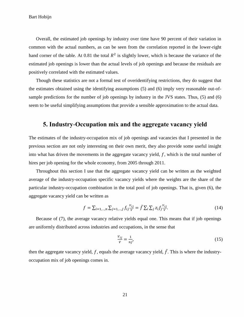
5. Industry-Occupation mix and the aggregate vacancy yield
The estimates of the industry-occupation mix of job openings and vacancies that I presented in the
previous section are not only interesting on their own merit, they also provide some useful insight
into what has driven the movements in the aggregate vacancy yield, , which is the total number of
hires per job opening for the whole economy, from 2005 through 2011.
Throughout this section I use that the aggregate vacancy yield can be written as the weighted
average of the industry-occupation specific vacancy yields where the weights are the share of the
particular industry-occupation combination in the total pool of job openings. That is, given (6), the
aggregate vacancy yield can be written as
∑ ∑
∑ ∑
. (14)
Because of (7), the average vacancy relative yields equal one. This means that if job openings
are uniformly distributed across industries and occupations, in the sense that
, (15)
then the aggregate vacancy yield, , equals the average vacancy yield, . This is where the industry-
occupation mix of job openings comes in.
The Mix of U.S. Job Openings and Hires
22
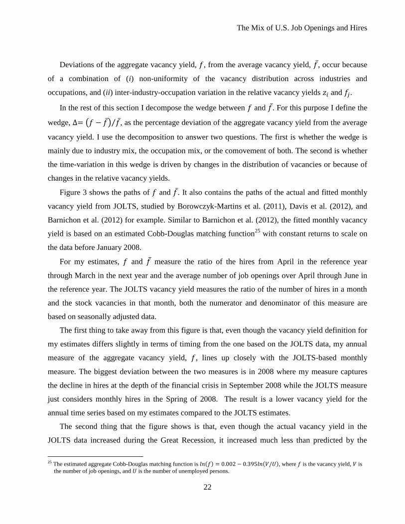
Deviations of the aggregate vacancy yield, , from the average vacancy yield, , occur because
of a combination of (i) non-uniformity of the vacancy distribution across industries and
occupations, and (ii) inter-industry-occupation variation in the relative vacancy yields and .
In the rest of this section I decompose the wedge between and . For this purpose I define the
wedge, ( ) ⁄ , as the percentage deviation of the aggregate vacancy yield from the average
vacancy yield. I use the decomposition to answer two questions. The first is whether the wedge is
mainly due to industry mix, the occupation mix, or the comovement of both. The second is whether
the time-variation in this wedge is driven by changes in the distribution of vacancies or because of
changes in the relative vacancy yields.
Figure 3 shows the paths of and . It also contains the paths of the actual and fitted monthly
vacancy yield from JOLTS, studied by Borowczyk-Martins et al. (2011), Davis et al. (2012), and
Barnichon et al. (2012) for example. Similar to Barnichon et al. (2012), the fitted monthly vacancy
yield is based on an estimated Cobb-Douglas matching function25
with constant returns to scale on
the data before January 2008.
For my estimates, and measure the ratio of the hires from April in the reference year
through March in the next year and the average number of job openings over April through June in
the reference year. The JOLTS vacancy yield measures the ratio of the number of hires in a month
and the stock vacancies in that month, both the numerator and denominator of this measure are
based on seasonally adjusted data.
The first thing to take away from this figure is that, even though the vacancy yield definition for
my estimates differs slightly in terms of timing from the one based on the JOLTS data, my annual
measure of the aggregate vacancy yield, , lines up closely with the JOLTS-based monthly
measure. The biggest deviation between the two measures is in 2008 where my measure captures
the decline in hires at the depth of the financial crisis in September 2008 while the JOLTS measure
just considers monthly hires in the Spring of 2008. The result is a lower vacancy yield for the
annual time series based on my estimates compared to the JOLTS estimates.
The second thing that the figure shows is that, even though the actual vacancy yield in the
JOLTS data increased during the Great Recession, it increased much less than predicted by the
25 The estimated aggregate Cobb-Douglas matching function is ( ) ( ), where is the vacancy yield, is
the number of job openings, and is the number of unemployed persons.
Bart Hobijn
23
estimated aggregate matching function. Before the start of the Great Recession in December 2007
the estimated aggregate Cobb-Douglas matching function fitted the vacancy yield well. However,
the out-of-sample prediction after the end of 2007 is not good. By the Spring of 2011 the fitted
vacancy yield was 27 percent higher than the actual vacancy yield. This suggests there was a
substantial decline in the efficiency with which the unemployed get matched with unfilled job
openings in the labor market. This result is not new.26
Barnichon et al. (2012) show that this decline
in aggregate match efficiency is the main source behind the rightward shift in the U.S. Beveridge
curve since 2008.
The final thing that stands out from the figure is that the estimated average vacancy yield lines
up closely with the fitted vacancy yield. Given that the aggregate vacancy yield from the JVS data
is similar to the actual monthly vacancy yield from the JOLTS data, this implies that the wedge
between the aggregate vacancy yield , and the average vacancy yield, , behaves very much like
the estimated decline in match efficiency in the monthly JOLTS data.
Table 8 contains the time series of and as well as the wedge, . As can be seen from the
table, in 2007 the aggregate vacancy yield was 5 percent below the average vacancy yield. In 2009
this gap peaked at 36 percent. By 2011 this gap had come down somewhat to 26 percent. On
average over the 2005-2007 period the aggregate vacancy yield was 16 percent lower than the
average vacancy yield while during the 2009-2011 period the gap was almost twice as big, at 31
percent. Thus, the shift in the industry-occupation mix of job openings and hires from before to
after the recession has substantially increased the wedge between the aggregate and average
vacancy yields, , to a degree that is similar to the estimated decline in aggregate match efficiency.
So, the observed decline in aggregate match efficiency is in large part accounted for by shift in the
mix of vacancies and hires.
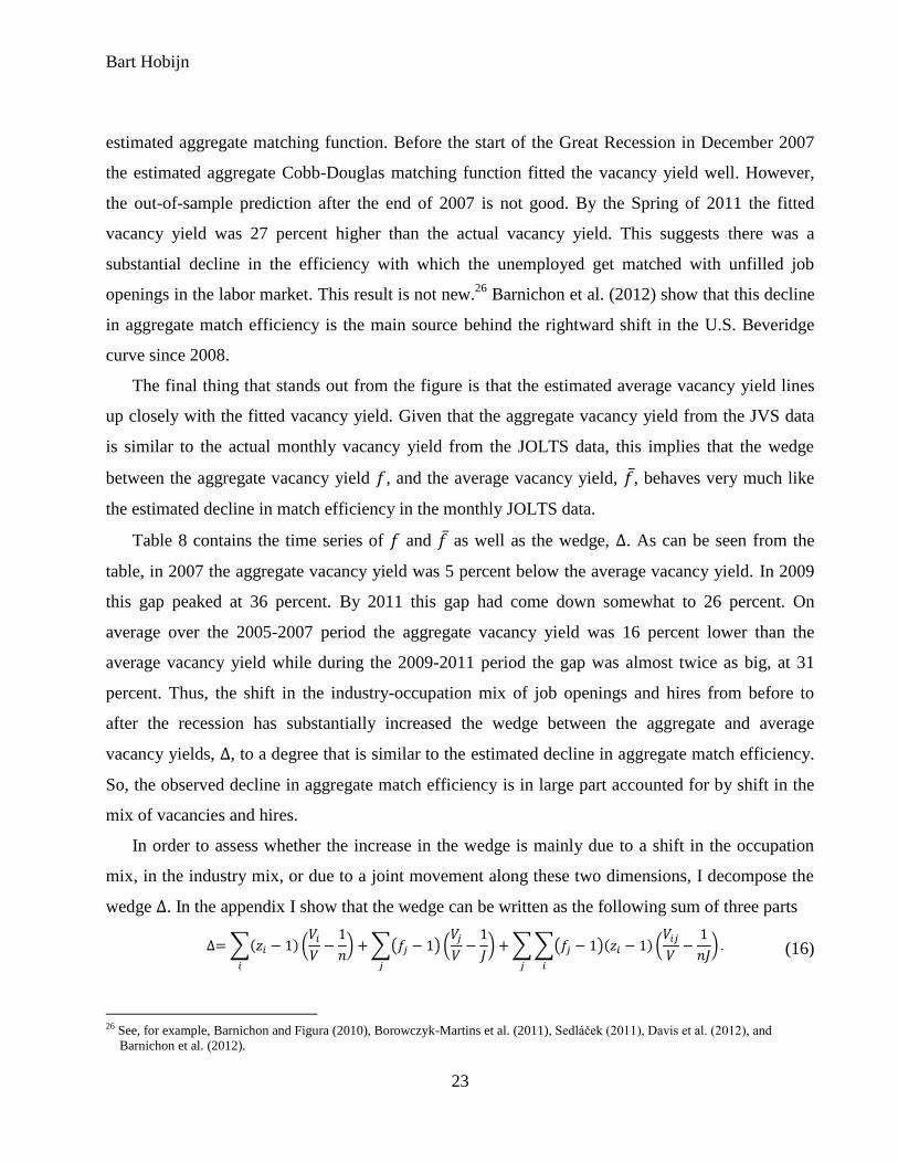
In order to assess whether the increase in the wedge is mainly due to a shift in the occupation
mix, in the industry mix, or due to a joint movement along these two dimensions, I decompose the
wedge . In the appendix I show that the wedge can be written as the following sum of three parts
∑( ) (
)
∑( ) (
)
∑∑( )( ) (
)
(16)
26 See, for example, Barnichon and Figura (2010), Borowczyk-Martins et al. (2011), Sedláček (2011), Davis et al. (2012), and
Barnichon et al. (2012).
The Mix of U.S. Job Openings and Hires
24
The first term on the right-hand side of this expression represents the impact of the cross-
industry composition of vacancies on the wedge, while the second term represents the impact of the
cross-occupation distribution of vacancies. The third term reflects whether the vacancy distribution
is shifted in such a way that the relative vacancy yields across industries and occupations are
correlated.
The last three columns of Table 8 show the decomposition of the wedge into the three right-
hand side parts of (16). These columns show that, on average, the industry mix of vacancies lowers
the aggregate vacancy yield relative to the average vacancy yield by 8 percent. The occupation mix
lowers it by 13 percent. The covariance term has only a small negative effect. Moreover, comparing
the averages for `05-`07 with those for `09-`11 the columns show that the increase in the wedge
since the start of the recession has been completely due to the shift in the occupation mix of
vacancies.27
Thus, a large part of the measured decline in aggregate match efficiency can be attributed to two
developments: (i) A shift in the distribution of vacancies towards occupations with lower relative
vacancy yields, and (ii) A decline in the relative vacancy yields of occupations with a higher than
average number of vacancies.
To quantify which of the occupational groups contribute most to this shift and which of the two
channels discussed above is driving this contribution, I consider the second part of the right-hand
side of (16) in more detail. From that part, it can be seen that the contribution of an occupation, say
, to the wedge equals
( ) .
/. (17)
Equation (17) implies that the contribution of each occupation can be gleaned from a scatter plot
of vacancy shares versus the relative vacancy yield by occupation. Figure 4 shows such a scatterplot
for both the `05-`07 and the `09-`11 periods. The horizontal dashed line in the figure is the line at
which and the vertical dashed line is that at which
.
27 This result is similar to the analysis of mismatch in the U.S. labor market by Şahin et al. (2011). They make much more specific
functional form assumptions about matching functions in particular subsections of the labor market and then calculate a formal
index of mismatch. Where I analyze the industry-occupation mix jointly, they construct separate indices for industries and
occupations and find that occupational mismatch is higher than mismatch across industries.

Bart Hobijn
25
Equation (17) implies that the contribution of an industry to the vacancy yield wedge is equal to
the size of the rectangle that has as one of its corners the data point and as another corner the
intersection of the two dashed lines.
If occupation has an above average relative vacancy yield, , but has a below average
vacancy share,
, then the average vacancy yield would increase if the vacancy distribution
would be more uniform. Thus, such an occupation reduces relative to . This is the case, for
example, for “Legal” positions, , which have a very small share in the total number of
vacancies (Table 2) but have a high rate of hires per vacancy (Table 3). In short, if more positions
were as easy to fill as those for “Legal” occupations this would raise the aggregate vacancy yield.
Just like , all occupations with observations in the upper-left quadrant of Figure 4 contribute
negatively to the vacancy yield wedge.
Reversely, an occupation with a high job openings share and a low relative vacancy yield also
contributes negatively to the wedge. This is, for example, the case for “Healthcare Practitioners and
Technical” jobs, . Other occupations in the lower right hand quadrant also make a negative
contribution to the wedge.
By a similar argument, all occupations in the lower-left and upper-right quadrants help to raise
the wedge. This is, for example, the case for “Office and Administrative Support” in the
upper-right quadrant and “Farming, Fishing, and Forestry” in the lower-left quadrant. There are,
however, very few observations in the upper-right quadrant. As a consequence, in every year the
observations in the upper-left and lower-right quadrants outweigh the other ones and the occupation
mix contribution to the vacancy yield wedge is negative.
As I showed in Table 8, from `09 through `11 the occupation mix dragged down the vacancy
yield wedge much more than before the Great Recession. The scatterplot of Figure 4 reveals which
occupations were the main drivers behind this. The movements of the six biggest contributors are
indicated by arrows. Vertical movements in the points associated with these occupations are
changes in the relative vacancy yields between `05-`07 and `09-`11. Horizontal movements are
changes in the vacancy shares.
The biggest contributor to the change in is “Legal” occupations, . This is because these
job openings became relatively much easier to fill after the recession than before it. The second
biggest contributor is made up of “Sales and Related” positions, , which increased their

The Mix of U.S. Job Openings and Hires
26
vacancy share by about 2 percentage points and became relatively hard to fill as compared to before
the recession. Next are “Construction and Extraction” job openings, , which saw a 2.8
percentage point decline in their vacancy share and went from relatively hard to fill to twice as easy
to fill as the average across occupations. After that, “Office and Administrative Support”, ,
has added most to the decline in the wedge because of the reduction in the positive contribution to
the wedge of this category. Finally, in fifth and sixth place are the two health care related
occupation categories, and . Both these groups did not see a big change in their low
relative vacancy yield but did see a substantial increase in their vacancy shares.
Implications
The results in this section show that the occupation mix of job openings has caused an increased
drag on the aggregate vacancy yield. This drag was caused by the changes in vacancy shares of
various occupations as well as through the relative ease with which job openings for different
occupations get filled. The industry-occupation mix of job openings and hires thus is an important
source of the decline in aggregate match efficiency that has resulted in the recent rightward shift in
the U.S. Beveridge curve.
Conventional models of the labor market with search frictions imply a temporary rightward shift
of the Beveridge curve at the depth of a recession (Mortensen, 1994) and such rightward shifts have
been observed in previous recessions. However, these models generate such shifts for a given level
of aggregate match efficiency and have a hard time explaining a shift as persistent as observed from
`09-`11 (and onwards).
As a result, the measured decline in aggregate match efficiency and the resulting rightward shift
in the Beveridge curve have been interpreted as a sign of an increased level of the natural rate of
unemployment (Kocherlakota, 2010). The analysis in this paper shines a new light on the source of
the decline in match efficiency; it is largely due to the change in the occupation mix of job openings
and hires.
Of course, my analysis does not directly address whether this shift in the mix of job openings is
permanent or largely transitory. However, the results by occupation do provide some insight into
this. As expected, the decline in the demand for construction workers and the increase in the relative
demand for healthcare workers have both been a drag on the aggregate vacancy yield. Because the

Bart Hobijn
27
demand for construction workers is not expected to recover to its pre-recession level and the shift in
demand to healthcare related occupations is indicative of an underlying long-run trend, this is likely
to put downward pressure on the number of hires per vacancy in the medium to long-run, pushing
up the natural rate of unemployment.
This is only part of the story. For the other occupations that contribute to the increase in the
vacancy wedge, which are “Legal”, “Sales and Related”, and “Office and Administrative Support”,
it is reasonable to expect their effect on the vacancy yield wedge to taper off when the labor market
recovers.
In this sense, my results are reminiscent of the discussion between Lilien (1982) and Abraham
and Katz (1986). Lilien (1982) argued that recessions are times of accelerated structural change
because at times of high unemployment the standard deviation of the growth rate of employment
across industries and unemployment rate across occupations spikes. This could be indicative of a
higher degree of cross-industry and occupation reallocation of labor during recessions than during
expansions.28
Instead, Abraham and Katz (1986) argue that these spikes in the standard deviation in
cross-industry employment growth rates are mostly due to differences in the cyclical sensitivity of
industries and do not capture structural reallocation patterns. They point out that most of these
spikes result in negative comovements between the unemployment and job openings rates and that
these negative comovements are driven by cyclical adjustments in the labor market rather than
structural changes.29
Just like increases in cross-industry variation in employment growth, drops in measured match
efficiency have been pointed to as signaling structural increases in labor market frictions. However,
my results indicate that a large part of the recent decline in measured match efficiency is driven by,
most likely, cyclical changes in the industry-occupation mix of job openings and hires. When the
labor market recovers and these shifts reverse measured match efficiency will rebound and the
Beveridge curve will shift inward.
Figure 3 and Table 8 show that some of this rebound has already taken place. The vacancy yield
wedge, , has gone from -36 percent in 2009 to – 26 percent in 2011. This is in line with the results
28 Recent evidence by Carrillo-Tudela and Visschers (2011) and Hobijn (2012) indicates that cross-occupational and cross-industry
mobility actually declines during recessions. 29 Hosios (1994) provides a counterexample. He uses a simple model to show that structural changes in the labor market could also
result in a negative correlation between the unemployment and vacancy rates.

The Mix of U.S. Job Openings and Hires
28
for industry-level and occupational-level mismatch in Şahin et al. (2011), which point to mismatch
having peaked in 2009. Of course, to what extent this rebound will continue remains to be seen.
6. Who is getting hired in which job openings?
Now that I have an estimate of which industries post vacancies for which occupations, the final
question is who actually gets hired in these vacancies. Does a manufacturer that posts a vacancy for
an administrative assistant tend to fill that vacancy with someone who used to work in
manufacturing and is that person likely to have been an administrative assistant in their previous
job?
This question differs from measures of labor market mobility commonly reported. Industry and
occupational mobility are generally measured as the percentage of workers changing industry and
occupation (Kambourov and Manovskii (2008), Moscarini and Thomsson (2008), and Bjelland et
al. (2010)). Less attention has been paid to the hires side. That is, what is the fraction of workers of
different occupations that get hired in particular job openings?
The answer to this question is important because it allows us to consider for which persons job
openings in particular industries and occupations are likely to provide job opportunities. To analyze
this question, I introduce estimates of cross-industry and cross-occupation hiring matrices for April
2005 through March 2012 in Tables 9 and 10 respectively.
These hiring matrices are constructed as follows. For the persons hired in industry in
occupation during a month who are still employed at the end of the month, , the CPS does not
only contain data on their new job. It also contains information on whether or not they have a
previous work history and, if so, in which industry and occupation they held their previous job.
Table 9 cross-tabulates the in terms of the industry in which the person gets hired versus
the industry in which he or she was previously employed for the hires that occurred between April
2005 and March 2012.30
The column sums of the table add up to 100 percent. To give an example,
the 5.1 percent in row 2 and column 3 indicates that one out of twenty persons hired in durables
manufacturing were previously employed in construction. Table 10 provides the same cross-
tabulation but then by occupation instead.
30 This is the same period over which I constructed the hires measures used to estimate the job openings by industry and occupation.
Bart Hobijn
29
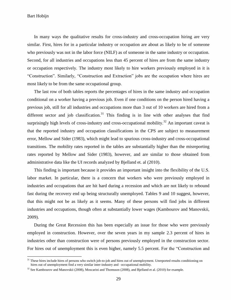
In many ways the qualitative results for cross-industry and cross-occupation hiring are very
similar. First, hires for in a particular industry or occupation are about as likely to be of someone
who previously was not in the labor force (NILF) as of someone in the same industry or occupation.
Second, for all industries and occupations less than 45 percent of hires are from the same industry
or occupation respectively. The industry most likely to hire workers previously employed in it is
“Construction”. Similarly, “Construction and Extraction” jobs are the occupation where hires are
most likely to be from the same occupational group.
The last row of both tables reports the percentages of hires in the same industry and occupation
conditional on a worker having a previous job. Even if one conditions on the person hired having a
previous job, still for all industries and occupations more than 3 out of 10 workers are hired from a
different sector and job classification.31
This finding is in line with other analyses that find
surprisingly high levels of cross-industry and cross-occupational mobility.32
An important caveat is
that the reported industry and occupation classifications in the CPS are subject to measurement
error, Mellow and Sider (1983), which might lead to spurious cross-industry and cross-occupational
transitions. The mobility rates reported in the tables are substantially higher than the misreporting
rates reported by Mellow and Sider (1983), however, and are similar to those obtained from
administrative data like the UI records analyzed by Bjelland et. al (2010).
This finding is important because it provides an important insight into the flexibility of the U.S.
labor market. In particular, there is a concern that workers who were previously employed in
industries and occupations that are hit hard during a recession and which are not likely to rebound
fast during the recovery end up being structurally unemployed. Tables 9 and 10 suggest, however,
that this might not be as likely as it seems. Many of these persons will find jobs in different
industries and occupations, though often at substantially lower wages (Kambourov and Manovskii,
2009).
During the Great Recession this has been especially an issue for those who were previously
employed in construction. However, over the seven years in my sample 2.3 percent of hires in
industries other than construction were of persons previously employed in the construction sector.
For hires out of unemployment this is even higher, namely 5.5 percent. For the “Construction and
31 These hires include hires of persons who switch job-to-job and hires out of unemployment. Unreported results conditioning on
hires out of unemployment find a very similar inter-industry and –occupational mobility. 32 See Kambourov and Manovskii (2008), Moscarini and Thomsson (2008), and Bjelland et al. (2010) for example.
The Mix of U.S. Job Openings and Hires
30
extraction” occupation, these percentages are 2.1 and 5.3 percent respectively. Thus, as the overall
labor market recovers these workers are likely to find jobs outside of construction.
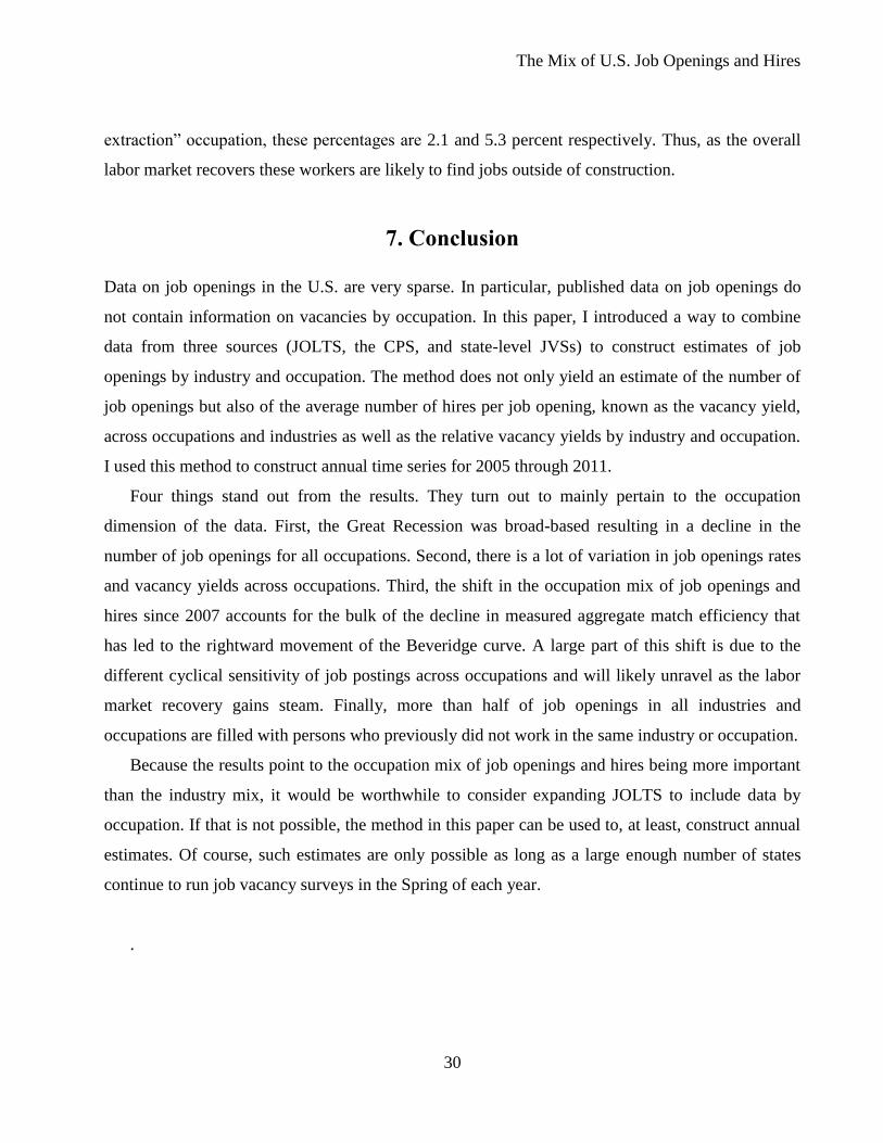
7. Conclusion
Data on job openings in the U.S. are very sparse. In particular, published data on job openings do
not contain information on vacancies by occupation. In this paper, I introduced a way to combine
data from three sources (JOLTS, the CPS, and state-level JVSs) to construct estimates of job
openings by industry and occupation. The method does not only yield an estimate of the number of
job openings but also of the average number of hires per job opening, known as the vacancy yield,
across occupations and industries as well as the relative vacancy yields by industry and occupation.
I used this method to construct annual time series for 2005 through 2011.
Four things stand out from the results. They turn out to mainly pertain to the occupation
dimension of the data. First, the Great Recession was broad-based resulting in a decline in the
number of job openings for all occupations. Second, there is a lot of variation in job openings rates
and vacancy yields across occupations. Third, the shift in the occupation mix of job openings and
hires since 2007 accounts for the bulk of the decline in measured aggregate match efficiency that
has led to the rightward movement of the Beveridge curve. A large part of this shift is due to the
different cyclical sensitivity of job postings across occupations and will likely unravel as the labor
market recovery gains steam. Finally, more than half of job openings in all industries and
occupations are filled with persons who previously did not work in the same industry or occupation.
Because the results point to the occupation mix of job openings and hires being more important
than the industry mix, it would be worthwhile to consider expanding JOLTS to include data by
occupation. If that is not possible, the method in this paper can be used to, at least, construct annual
estimates. Of course, such estimates are only possible as long as a large enough number of states
continue to run job vacancy surveys in the Spring of each year.
.
Bart Hobijn
31
References
Abraham, Katharine G., and Lawrence F. Katz (1986), “Cyclical Unemployment: Sectoral Shifts or
Aggregate Disturbances?” Journal of Political Economy, 94, 507-522.
Abraham, Katharine G. (1987) “Help Wanted Advertising, Job Vacancies and Unemployment,”
Brookings Papers on Economic Activity, 207-243.
Barnichon, Regis (2010), “Building a composite Help-Wanted Index,” Economics Letters, 109(3),
175-178.
Barnichon, Regis, and Andrew Figura (2010), “What Drives Movements in the Unemployment
Rate? A Decomposition of the Beveridge Curve,” Finance and Economics Discussion Series
2010-48, Federal Reserve Board of Governors.
Barnichon, Regis, Michael W.L. Elsby, Bart Hobijn, and Ayșegül Șahin (2012) “Which Industries
are Shifting the Beveridge Curve?” Monthly Labor Review, June, 25-37.
Bjelland, Melissa, Bruce Fallick, John C. Haltiwanger, and Erika McEntarfer (2010) “Employer-to-
Employer Flows in the United States: Estimates Using Linked Employer-Employee Data,”
Center for Economic Studies Working Paper 10-26.
Borowczyk-Martins, Daniel, Grégory Jolivet, and Fabien Postel-Vinay (2011) “Accounting For
Endogenous Search Behavior in Matching Function Estimation,” mimeo, University of Bristol.
Carrillo-Tudela, Carlos, and Ludo Visschers (2011), “Unemployment and Endogenous Reallocation
over the Business Cycle,” mimeo.
Clayton, Richard L., James R. Spletzer, and John C. Wohlford (2011) “Conference Report: JOLTS
Symposium,” Monthly Labor Review, February, 40-47.
Coles, Melvyn G. and Eric Smith (1996), “Cross-Section Estimation of the Matching Function:
Evidence from England and Wales,” Economica, 63, 589-597.
Daly, Mary C., Bart Hobijn, Ayșegül Șahin, and Robert G. Valletta (2012), “A Search and
Matching Approach to Labor Markets: Is the Natural Rate of Unemployment Rising?” Journal
of Economic Perspectives, forthcoming.
Davis, Steven J., R. Jason Faberman, John C. Haltiwanger, and Ian Rucker (2008), “Adjusted
Estimates of Worker Flows and Job Openings in JOLTS,” NBER Working Paper No. 14137.
Davis, Steven J., R. Jason Faberman, and John C. Haltiwanger (2010), “The Establishment-Level
Behavior of Vacancies and Hiring,” NBER Working Paper No. 16265.
Davis, Steven J., R. Jason Faberman, and John C. Haltiwanger (2012) “Recruiting Intensity during
and after the Great Recession: National and Industry Evidence,” American Economic Review:
Papers and Proceedings, forthcoming.
Dickens, William T. (2009), “A New Method for Estimating Time Variation in the NAIRU,”
Understanding Inflation and the Implications for Monetary Policy: A Phillips Curve
Retrospective, 205-228, MIT press.

The Mix of U.S. Job Openings and Hires
32
Dickens, William T., and Robert K. Triest (2012), “Potential Effects of the Great Recession on the
U.S. Labor Market,” B.E. Journal of Macroeconomics, forthcoming.
Elsby, Michael W.L., Bart Hobijn, and Ayșegül Șahin (2010), “The Labor Market in the Great
Recession,” Brookings Papers on Economic Activity, Spring 2010, 1-48.
Fallick, Bruce, and Charles A. Fleischman (2004), “Employer-to-Employer Flows in the U.S. Labor
Market: The Complete Picture of Gross Worker Flows.” Finance and Economics Discussion
Series 2004-34. Washington: Board of Governors of the Federal Reserve System.
Ferber, Robert (ed.) (1966), The Measurement and Interpretation of Job Vacancies, National
Bureau of Economic Research, New York: Columbia University Press.
Hobijn, Bart (2012), “Comments on Potential Effects of the Great Recession on the U.S. Labor
Market, by William T. Dickens and Robert K. Triest,” Berkeley Electronic Journal:
Macroeconomics, forthcoming.
Hosios, Arthur J. (1994), “Unemployment and Vacancies with Sectoral Shifts,” American Economic
Review, 84, 124-144.
Jovanovic, Boyan (1979), “Job Matching and the Theory of Turnover,” Journal of Political
Economy, 87, 972-990.
Kambourov, Gueorgui, and Iourii Manovskii (2008), “Rising Occupational and Industry Mobility in
the United States: 1968-1997,” International Economic Review, 49, 41-79.
Kambourov, Gueorgui, and Iourii Manovskii (2009), “Occupational Mobility and Wage
Inequality,” Review of Economic Studies, 76, 731-759.
Kocherlakota, Narayana (2010). “Inside the FOMC,” Speech at Marquette, Michigan, August 17,
2010.
Lilien, David M. (1982), “Sectoral Shifts and Cyclical Unemployment,” Journal of Political
Economy, 777-793.
Lubik, Thomas A. (2011), “The Shifting and Twisting Beveridge Curve: An Aggregate
Perspective,” mimeo, Federal Reserve Bank of Richmond.
Mellow, Wesley, and Hal Sider (1983), “Accuracy of Response in Labor Market Surveys: Evidence
and Implications,” Journal of Labor Economics, 1, 331-344.
Mortensen, Dale T. (1994), “The Cyclical Behavior of Job and Worker Flows,” Journal of
Economic Dynamics and Control, 18, 1121-1142.
Mortensen, Dale T., and Christopher A. Pissarides (1994), “Job Creation and Job Destruction in the
Theory of Unemployment,” The Review of Economic Studies, 61, 397-415.
Moscarini, Guiseppe, and Thomsson, Kaj (2008), “Occupational and Job Mobility in the US,”
Scandinavian Journal of Economics , 109 (4), 807-836.
Nagypál, Éva (2008), “Worker Reallocation over the Business Cycle: The Importance of Job-to-Job
Transitions,” mimeo, Northwestern University.
Petrongolo, Barbara, and Christopher A. Pissarides (2001), “Looking into the Black Box: A Survey
of the Matching Function.” Journal of Economic Literature, 39, 390-431.

Bart Hobijn
33
Șahin, Ayșegül, Joseph Song, Giorgio Topa, and Gianluca Violante (2011), “Measuring Mismatch
in the U.S. Labor Market,” mimeo, New York University.
Sedláček, Petr (2011), “Match Efficiency and the Cyclical Behavior of Job Finding Rates,” mimeo,
http://www.psedlacek.com/Documents/Working/Sedlacek_MatchEfficiency.pdf
Shimer, Robert (2012), "Reassessing the Ins and Outs of Unemployment," Review of Economic
Dynamics, 15, 127-148.
Sterk, Vincent (2010), “Home Equity, Mobility, and Macroeconomic Fluctuations,” DNB Working
Paper No. 265.
Valletta, Robert G. (2005), “Why Has the U.S. Beveridge Curve Shifted Back? New Evidence
Using Regional Data,” FRBSF Working Paper 2005-25, Federal Reserve Bank of San
Francisco.
A. Mathematical details
Continuous-time vacancy-flow model
The following is essentially a continuous-time version of the vacancy-flow model presented in
Davis, Faberman, and Haltiwanger (2010). I develop the model at the joint industry, indexed by ,
and occupation, indexed by , level. I denote time by the subscript and assume it to be measured in
months. In particular, I consider a representative month, for which ( -.
In terms of notation, is the number of job openings in industry for jobs of occupation .
is the number of persons hired by industry in occupation since the beginning of the month,
i.e. since . This also means that by definition. To match the JOLTS data with data on
labor market flows from the CPS, I define as the number of persons hired in ( ) since the
beginning of the month who are still in the job at time . Just like for hires, since is a flow
variable, .
Similar to Davis, Faberman, and Haltiwanger (2010), the model I use describes the laws of
motion of , , and as a function of hazard and arrival rates.33
I assume that these hazard
and arrival rates are constant over the month we consider. Therefore, I drop their time-subscript.
33 Davis, Faberman, and Haltiwanger (2010) write these laws-of-motion in discrete time that evolves with daily increments. It turns
out that, for the purpose of my analysis, it is more convenient to write them in continuous time where the hazard and arrival rates
are measured in monthly terms.

The Mix of U.S. Job Openings and Hires
34
These rates are defined as follows. Vacancies get filled at the rate and unfilled vacancies get
dropped at the rate . New vacancies are opened at the rate . Workers separate from their jobs,
either because they get laid off, quit, retire, die, emigrate, join the armed forces, etc., at rate .
This means that, at any point in time, the number of vacancies changes for three reasons. First,
some of them get filled. Second, some of them get dropped. Third, new vacancies are added. This
allows me to write the change in the number of vacancies as
( ) . (18)
The change in the number of hires since the beginning of the month is the number of vacancies that
get filled. That is
. (19)
Finally, the change in the number of persons hired since the beginning of the month, who are still
employed at time is given by the new hires at that time, minus those who are leaving their jobs.
That is,
. (20)
These are three differential equations that guide the vacancy and hiring flows. The model is
completed by the initial conditions, , and the given initial level of job openings,
.
The solution to this system of differential equations is the following. Vacancies evolve
according to
( ) ( ), where
. (21)
Here, is the steady-state level of vacancies. Substituting this solution into the law of motion of
hires, (19), yields
0 ( ) 1( ). (22)
Moreover, substituting (21) into (20), results in
, -
0 ( ) 1( ). (23)

Bart Hobijn
35
The general solution derived above depends on the deviation of the level of vacancies at the start of
the month from its steady state. To keep our analysis tractable, I limit myself to the steady-state
solution of this system for the empirical application in the main text.
Steady-state solution of vacancy-flow model: Equations (3) and (5) in main text
The stock of vacancies is a jump variable. If, at the beginning of the month, firms adjust their level
of job openings such that they are constant over the month, then they set . Under this
steady-state assumption, the solution of the model becomes very simple.
Since the model is in steady state, the number of vacancies is constant over time. That is
, for ( -. (24)
The number of hires over the month then equals the fill rate times the number of vacancies
. (25)
This means that the number of hires per vacancy, ⁄ , also known as the vacancy yield,
simply equals . This is why I denote the vacancy yield by in the main text. The number of
workers at the end of the month who have been hired during the month, under the steady-state
assumption, equals
, -
. (26)
The above two equations coincide equations (3) and (5) I use in the main text. There, I do not use
the time subscript and drop it from the equations.
Constructing hires from the CPS
From (4) I find that
(
). (27)
Equation (3) implies that
. (28)
Combining these two gives

The Mix of U.S. Job Openings and Hires
36
( ) ( )
⁄ . (29)
This is what allows me to get a measure of hires in industry and occupation using data from the
CPS. In practice, calculation of by industry and occupation results in unreliable estimates due to
very few observations for some industry-occupation combinations. To deal with this problem, I pool
the data across industries and just calculate a separation rate by occupation. The estimates, , are
reported in Table A.1.
Method of moment estimates
Combining (1) and (2) and the fact that our parameterization of the vacancy yields, (5), gives
∑ ∑
for , (30)
and
∑
∑
for . (31)
Writing these equations in terms of the relative vacancy yields, I obtain
∑
for . (32)
and
∑
for . (33)
Using the normalization restriction, (7), for the relative vacancy yields by occupation and (32)
allows me to write
∑ {
∑
}
∑
∑ {
∑
}
(34)
This is equation (8) in the main text. Except for the relative vacancy yields by occupation, the ‟s,
all other variables in this equation are measured from the data. So, I use this equation to obtain point
estimates of the relative vacancy yields by occupation.
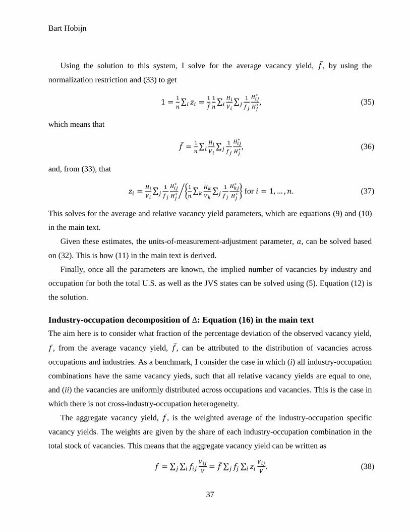
Bart Hobijn
37
Using the solution to this system, I solve for the average vacancy yield, , by using the
normalization restriction and (33) to get
∑
∑
∑
, (35)
which means that
∑
∑
, (36)
and, from (33), that
∑
{
∑
∑
}⁄ for . (37)
This solves for the average and relative vacancy yield parameters, which are equations (9) and (10)
in the main text.
Given these estimates, the units-of-measurement-adjustment parameter, , can be solved based
on (32). This is how (11) in the main text is derived.
Finally, once all the parameters are known, the implied number of vacancies by industry and
occupation for both the total U.S. as well as the JVS states can be solved using (5). Equation (12) is
the solution.
Industry-occupation decomposition of : Equation (16) in the main text
The aim here is to consider what fraction of the percentage deviation of the observed vacancy yield,
, from the average vacancy yield, , can be attributed to the distribution of vacancies across
occupations and industries. As a benchmark, I consider the case in which (i) all industry-occupation
combinations have the same vacancy yieds, such that all relative vacancy yields are equal to one,
and (ii) the vacancies are uniformly distributed across occupations and vacancies. This is the case in
which there is not cross-industry-occupation heterogeneity.
The aggregate vacancy yield, , is the weighted average of the industry-occupation specific
vacancy yields. The weights are given by the share of each industry-occupation combination in the
total stock of vacancies. This means that the aggregate vacancy yield can be written as
∑ ∑
∑ ∑
. (38)

The Mix of U.S. Job Openings and Hires
38
Using that the vacancy shares add up to one and that the respective average vacancy yields
across occupations and industries are also one, allows me to write
∑ ∑
∑∑( )
∑∑( )
∑( )∑( )
∑( ) (
)
∑( ) (
)
∑∑( )( ) (
)
(39)
Thus, the percentage deviation of the observed vacancy yield from the average vacancy yield can be
expressed as
∑( ) (
)
∑( ) (
)
∑∑( )( ) (
)
(40)
Which is equation (16) in the main text.
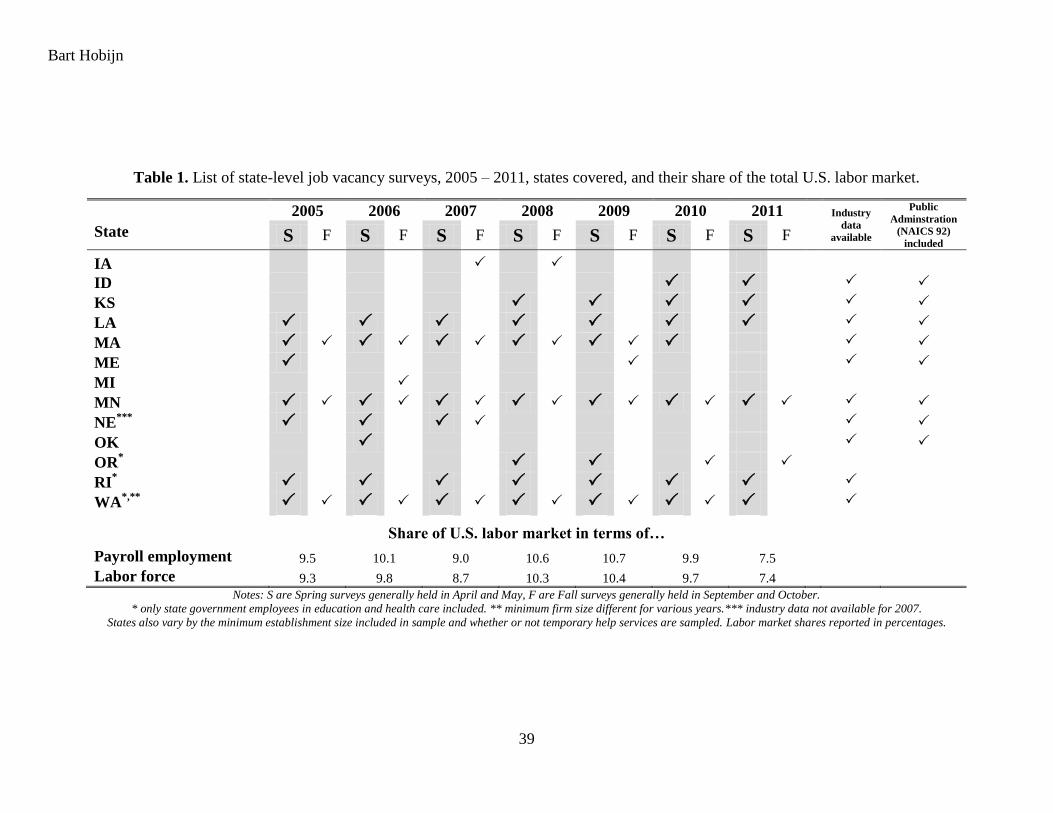
Bart Hobijn
39
Table 1. List of state-level job vacancy surveys, 2005 – 2011, states covered, and their share of the total U.S. labor market.
2005 2006 2007 2008 2009 2010 2011 Industry
data
available
Public
Adminstration
(NAICS 92)
included State S F S F S F S F S F S F S F
IA
ID
KS
LA
MA
ME
MI
MN
NE***
OK
OR*
RI*
WA*,**
Share of U.S. labor market in terms of…
Payroll employment 9.5 10.1 9.0 10.6 10.7 9.9 7.5
Labor force 9.3 9.8 8.7 10.3 10.4 9.7 7.4 Notes: S are Spring surveys generally held in April and May, F are Fall surveys generally held in September and October.
* only state government employees in education and health care included. ** minimum firm size different for various years.*** industry data not available for 2007.
States also vary by the minimum establishment size included in sample and whether or not temporary help services are sampled. Labor market shares reported in percentages.
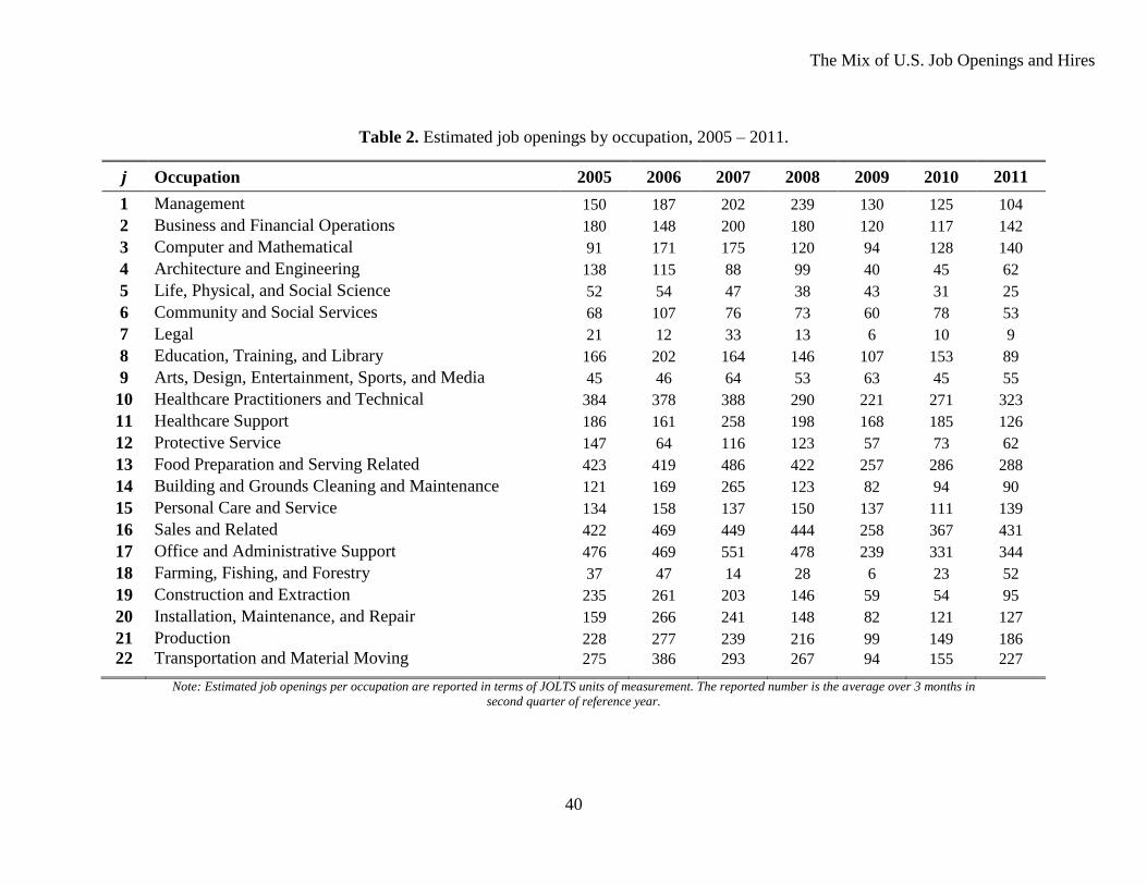
The Mix of U.S. Job Openings and Hires
40
Table 2. Estimated job openings by occupation, 2005 – 2011.
Occupation 2005 2006 2007 2008 2009 2010 2011
1 Management 150 187 202 239 130 125 104
2 Business and Financial Operations 180 148 200 180 120 117 142
3 Computer and Mathematical 91 171 175 120 94 128 140
4 Architecture and Engineering 138 115 88 99 40 45 62
5 Life, Physical, and Social Science 52 54 47 38 43 31 25
6 Community and Social Services 68 107 76 73 60 78 53
7 Legal 21 12 33 13 6 10 9
8 Education, Training, and Library 166 202 164 146 107 153 89
9 Arts, Design, Entertainment, Sports, and Media 45 46 64 53 63 45 55
10 Healthcare Practitioners and Technical 384 378 388 290 221 271 323
11 Healthcare Support 186 161 258 198 168 185 126
12 Protective Service 147 64 116 123 57 73 62
13 Food Preparation and Serving Related 423 419 486 422 257 286 288
14 Building and Grounds Cleaning and Maintenance 121 169 265 123 82 94 90
15 Personal Care and Service 134 158 137 150 137 111 139
16 Sales and Related 422 469 449 444 258 367 431
17 Office and Administrative Support 476 469 551 478 239 331 344
18 Farming, Fishing, and Forestry 37 47 14 28 6 23 52
19 Construction and Extraction 235 261 203 146 59 54 95
20 Installation, Maintenance, and Repair 159 266 241 148 82 121 127
21 Production 228 277 239 216 99 149 186
22 Transportation and Material Moving 275 386 293 267 94 155 227
Note: Estimated job openings per occupation are reported in terms of JOLTS units of measurement. The reported number is the average over 3 months in
second quarter of reference year.
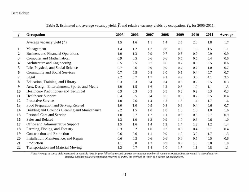
Bart Hobijn
41
Table 3. Estimated and average vacancy yield, , and relative vacancy yields by occupation, , for 2005-2011.
Occupation 2005 2006 2007 2008 2009 2010 2011 Average
Average vacancy yield ( ) 1.5 1.6 1.1 1.4 2.5 2.0 1.8 1.7
1 Management 1.4 1.2 1.2 0.8 0.8 1.0 1.5 1.1
2 Business and Financial Operations 1.0 1.3 0.9 0.7 0.8 0.9 0.9 0.9
3 Computer and Mathematical 0.9 0.5 0.6 0.6 0.5 0.5 0.4 0.6
4 Architecture and Engineering 0.5 0.5 0.7 0.6 0.7 0.8 0.5 0.6
5 Life, Physical, and Social Science 0.7 0.6 0.9 0.9 0.4 0.7 1.0 0.7
6 Community and Social Services 0.7 0.5 0.8 1.0 0.5 0.4 0.7 0.7
7 Legal 2.2 3.7 1.7 4.1 4.9 3.6 4.1 3.5
8 Education, Training, and Library 0.3 0.3 0.4 0.4 0.3 0.2 0.5 0.3
9 Arts, Design, Entertainment, Sports, and Media 1.9 1.5 1.6 1.2 0.6 1.0 1.1 1.3
10 Healthcare Practitioners and Technical 0.3 0.3 0.3 0.5 0.3 0.2 0.3 0.3
11 Healthcare Support 0.4 0.5 0.4 0.5 0.3 0.2 0.5 0.4
12 Protective Service 1.0 2.6 1.4 1.2 1.6 1.4 1.7 1.6
13 Food Preparation and Serving Related 1.0 1.0 0.9 0.8 0.6 0.4 0.6 0.7
14 Building and Grounds Cleaning and Maintenance 2.2 1.5 1.0 1.8 1.6 1.6 1.8 1.6
15 Personal Care and Service 1.0 0.7 1.2 1.1 0.6 0.8 0.7 0.9
16 Sales and Related 1.3 1.0 1.2 0.9 1.0 0.6 0.6 1.0
17 Office and Administrative Support 1.5 1.6 1.4 1.2 1.4 1.3 1.2 1.4
18 Farming, Fishing, and Forestry 0.3 0.2 1.0 0.3 0.8 0.4 0.1 0.4
19 Construction and Extraction 0.6 0.6 1.1 0.9 1.0 3.2 1.7 1.3
20 Installation, Maintenance, and Repair 0.6 0.3 0.6 0.6 0.6 0.5 0.5 0.6
21 Production 1.1 0.8 1.3 0.9 0.9 1.0 0.8 1.0
22 Transportation and Material Moving 1.2 0.7 1.4 1.0 1.7 1.1 0.8 1.1
Note: Average vacancy yield measured as monthly hires in year following second quarter per average number of vacancies outstanding per month in second quarter.
Relative vacancy yield of occupation reported as index, the average of which is 1 across all occupations.
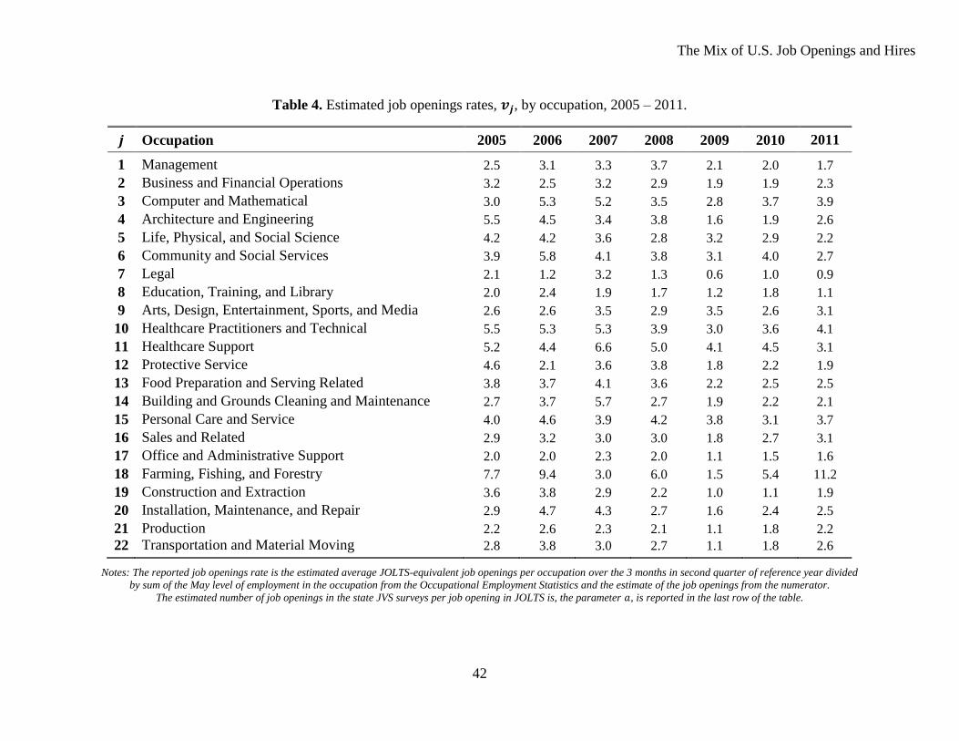
The Mix of U.S. Job Openings and Hires
42
Table 4. Estimated job openings rates, , by occupation, 2005 – 2011.
Occupation 2005 2006 2007 2008 2009 2010 2011
1 Management 2.5 3.1 3.3 3.7 2.1 2.0 1.7
2 Business and Financial Operations 3.2 2.5 3.2 2.9 1.9 1.9 2.3
3 Computer and Mathematical 3.0 5.3 5.2 3.5 2.8 3.7 3.9
4 Architecture and Engineering 5.5 4.5 3.4 3.8 1.6 1.9 2.6
5 Life, Physical, and Social Science 4.2 4.2 3.6 2.8 3.2 2.9 2.2
6 Community and Social Services 3.9 5.8 4.1 3.8 3.1 4.0 2.7
7 Legal 2.1 1.2 3.2 1.3 0.6 1.0 0.9
8 Education, Training, and Library 2.0 2.4 1.9 1.7 1.2 1.8 1.1
9 Arts, Design, Entertainment, Sports, and Media 2.6 2.6 3.5 2.9 3.5 2.6 3.1
10 Healthcare Practitioners and Technical 5.5 5.3 5.3 3.9 3.0 3.6 4.1
11 Healthcare Support 5.2 4.4 6.6 5.0 4.1 4.5 3.1
12 Protective Service 4.6 2.1 3.6 3.8 1.8 2.2 1.9
13 Food Preparation and Serving Related 3.8 3.7 4.1 3.6 2.2 2.5 2.5
14 Building and Grounds Cleaning and Maintenance 2.7 3.7 5.7 2.7 1.9 2.2 2.1
15 Personal Care and Service 4.0 4.6 3.9 4.2 3.8 3.1 3.7
16 Sales and Related 2.9 3.2 3.0 3.0 1.8 2.7 3.1
17 Office and Administrative Support 2.0 2.0 2.3 2.0 1.1 1.5 1.6
18 Farming, Fishing, and Forestry 7.7 9.4 3.0 6.0 1.5 5.4 11.2
19 Construction and Extraction 3.6 3.8 2.9 2.2 1.0 1.1 1.9
20 Installation, Maintenance, and Repair 2.9 4.7 4.3 2.7 1.6 2.4 2.5
21 Production 2.2 2.6 2.3 2.1 1.1 1.8 2.2
22 Transportation and Material Moving 2.8 3.8 3.0 2.7 1.1 1.8 2.6
Notes: The reported job openings rate is the estimated average JOLTS-equivalent job openings per occupation over the 3 months in second quarter of reference year divided
by sum of the May level of employment in the occupation from the Occupational Employment Statistics and the estimate of the job openings from the numerator.
The estimated number of job openings in the state JVS surveys per job opening in JOLTS is, the parameter , is reported in the last row of the table.
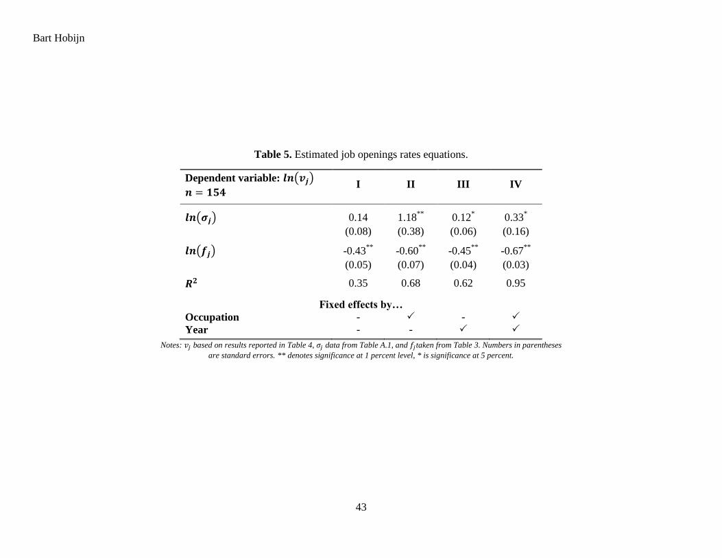
Bart Hobijn
43
Table 5. Estimated job openings rates equations.
Dependent variable: ( )
I II III IV
( ) 0.14 1.18**
0.12*
0.33*
(0.08) (0.38) (0.06) (0.16)
( ) -0.43**
-0.60**
-0.45**
-0.67**
(0.05)
(0.07) (0.04) (0.03)
0.35 0.68 0.62 0.95
Fixed effects by…
Occupation - -
Year - -
Notes: based on results reported in Table 4, data from Table A.1, and taken from Table 3. Numbers in parentheses
are standard errors. ** denotes significance at 1 percent level, * is significance at 5 percent.
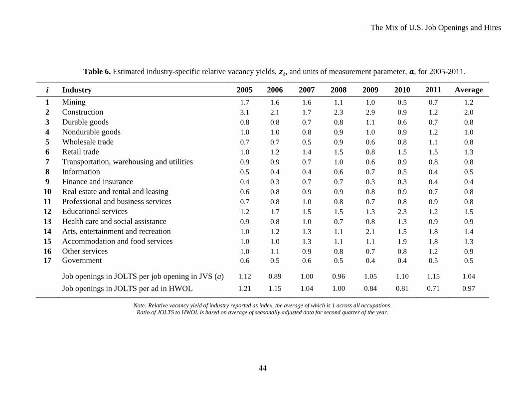
The Mix of U.S. Job Openings and Hires
44
Table 6. Estimated industry-specific relative vacancy yields, , and units of measurement parameter, , for 2005-2011.
Industry 2005 2006 2007 2008 2009 2010 2011 Average
1 Mining 1.7 1.6 1.6 1.1 1.0 0.5 0.7 1.2
2 Construction 3.1 2.1 1.7 2.3 2.9 0.9 1.2 2.0
3 Durable goods 0.8 0.8 0.7 0.8 1.1 0.6 0.7 0.8
4 Nondurable goods 1.0 1.0 0.8 0.9 1.0 0.9 1.2 1.0
5 Wholesale trade 0.7 0.7 0.5 0.9 0.6 0.8 1.1 0.8
6 Retail trade 1.0 1.2 1.4 1.5 0.8 1.5 1.5 1.3
7 Transportation, warehousing and utilities 0.9 0.9 0.7 1.0 0.6 0.9 0.8 0.8
8 Information 0.5 0.4 0.4 0.6 0.7 0.5 0.4 0.5
9 Finance and insurance 0.4 0.3 0.7 0.7 0.3 0.3 0.4 0.4
10 Real estate and rental and leasing 0.6 0.8 0.9 0.9 0.8 0.9 0.7 0.8
11 Professional and business services 0.7 0.8 1.0 0.8 0.7 0.8 0.9 0.8
12 Educational services 1.2 1.7 1.5 1.5 1.3 2.3 1.2 1.5
13 Health care and social assistance 0.9 0.8 1.0 0.7 0.8 1.3 0.9 0.9
14 Arts, entertainment and recreation 1.0 1.2 1.3 1.1 2.1 1.5 1.8 1.4
15 Accommodation and food services 1.0 1.0 1.3 1.1 1.1 1.9 1.8 1.3
16 Other services 1.0 1.1 0.9 0.8 0.7 0.8 1.2 0.9
17 Government 0.6 0.5 0.6 0.5 0.4 0.4 0.5 0.5
Job openings in JOLTS per job opening in JVS (a) 1.12 0.89 1.00 0.96 1.05 1.10 1.15 1.04
Job openings in JOLTS per ad in HWOL 1.21 1.15 1.04 1.00 0.84 0.81 0.71 0.97
Note: Relative vacancy yield of industry reported as index, the average of which is 1 across all occupations.
Ratio of JOLTS to HWOL is based on average of seasonally adjusted data for second quarter of the year.
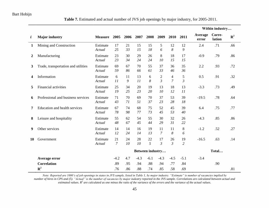
Bart Hobijn
45
Table 7. Estimated and actual number of JVS job openings by major industry, for 2005-2011.
Within industry…
Major industry Measure 2005 2006 2007 2008 2009 2010 2011 Average
error
Corre-
lation R
2
1 Mining and Construction Estimate 17 21 15 15 5 12 12 2.4 .71 .66
Actual 25 33 15 18 6 8 9
2 Manufacturing Estimate 23 30 29 26 8 18 17 -0.9 .79 .86
Actual 23 34 24 24 10 15 15
3 Trade, transportation and utilities Estimate 69 67 70 55 37 36 35 2.2 .93 .72
Actual 59 86 66 61 33 46 36
4 Information Estimate 6 11 13 6 2 4 5 0.5 .91 .32
Actual 11 9 11 8 3 7 3
5 Financial activities Estimate 25 34 20 19 13 18 13 -3.3 .73 .49
Actual 19 25 23 20 10 12 11
6 Professional and business services Estimate 71 70 69 70 37 53 39 -19.5 .78 .64
Actual 43 71 51 37 23 28 18
7 Education and health services Estimate 67 74 68 75 52 45 39 6.4 .75 .77
Actual 78 98 77 73 45 53 40
8 Leisure and hospitality Estimate 55 62 54 55 30 32 26 -4.3 .85 .86
Actual 48 67 45 44 29 31 22
9 Other services Estimate 14 14 16 19 11 11 8 -1.2 .52 .27
Actual 12 24 14 13 7 8 6
10 Government Estimate 21 24 28 22 17 26 19 -16.5 .63 .14
Actual 7 10 10 5 3 3 2
Between industry…
Total…
Average error -4.2 4.7 -4.3 -6.1 -4.3 -4.5 -5.1 -3.4
Correlation .89 .95 .94 .88 .94 .77 .84 .90
R2 .76 .86 .88 .74 .85 .58 .69 .81
Note: Reported are 1000’s of job openings in states in JVS sample, listed in Table 1, by major industry. “Estimate” is number of vacancies implied by
number of hires in CPS and (5). “Actual” is the number of vacancies by major industry reported in the JVS sample. Correlations are calculated between actual and
estimated values. R2 are calculated as one minus the ratio of the variance of the errors and the variance of the actual values.
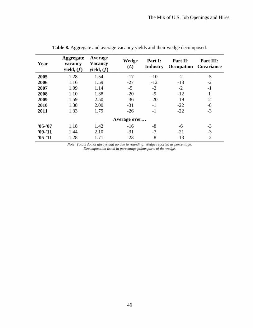
The Mix of U.S. Job Openings and Hires
46
Table 8. Aggregate and average vacancy yields and their wedge decomposed.
Year
Aggregate
vacancy
yield, ( )
Average
Vacancy
yield, ( )
Wedge
( )
Part I:
Industry
Part II:
Occupation
Part III:
Covariance
2005 1.28 1.54 -17 -10 -2 -5
2006 1.16 1.59 -27 -12 -13 -2
2007 1.09 1.14 -5 -2 -2 -1
2008 1.10 1.38 -20 -9 -12 1
2009 1.59 2.50 -36 -20 -19 2
2010 1.38 2.00 -31 -1 -22 -8
2011 1.33 1.79 -26 -1 -22 -3
Average over…
'05-'07 1.18 1.42 -16 -8 -6 -3
'09-'11 1.44 2.10 -31 -7 -21 -3
'05-'11 1.28 1.71 -23 -8 -13 -2
Note: Totals do not always add up due to rounding. Wedge reported as percentage.
Decomposition listed in percentage points parts of the wedge.

Bart Hobijn
47
Table 9. Cross-industry hiring matrix, April 2005 – March 2012.
Hiring industry
Previous industry/status 1 2 3 4 5 6 7 8 9 10 11 12 13 14 15 16 17
1 Mining 35.3 0.4 0.2 0.2 0.5 0.1 0.4 0.0 0.1 0.0 0.2 0.0 0.0 0.1 0.0 0.1 0.1
2 Construction 7.8 42.3 5.1 3.2 3.5 2.2 5.0 2.6 1.1 2.8 3.3 0.7 0.7 1.5 1.8 2.9 1.7
3 Durable goods 4.1 2.8 31.8 5.2 4.6 1.7 2.7 2.3 1.1 1.6 3.2 0.6 0.8 0.6 1.0 1.9 1.0
4 Nondurable goods 2.7 1.2 3.5 24.4 4.7 1.2 1.3 1.2 0.7 0.7 1.9 0.3 0.7 0.3 0.9 1.0 0.7
5 Wholesale trade 1.6 0.9 1.8 2.6 14.9 1.5 1.9 1.1 0.6 0.8 0.9 0.2 0.4 0.6 0.4 0.7 0.4
6 Retail trade 2.8 3.2 4.7 5.2 9.9 21.9 4.9 5.9 6.0 4.7 5.4 2.8 3.8 4.7 5.8 5.3 3.4
7 Transportation, warehousing and utilities 3.9 1.8 2.1 1.7 3.4 1.2 27.1 1.2 0.8 1.5 1.7 0.7 0.6 0.7 0.7 1.3 1.2
8 Information 0.7 0.6 0.7 0.8 0.7 0.8 0.6 22.5 1.3 0.7 1.2 0.5 0.4 1.4 0.5 0.6 0.9
9 Finance and insurance 0.3 0.3 0.8 0.8 1.3 0.9 0.7 1.6 30.7 1.9 2.2 0.7 0.9 0.6 0.5 0.7 1.1
10 Real estate and rental and leasing 0.7 0.6 0.5 0.3 0.7 0.6 0.8 0.4 1.1 19.3 0.8 0.3 0.5 0.4 0.4 0.5 0.7
11 Professional and business services 4.9 3.8 6.1 5.7 5.8 3.6 4.5 6.9 6.1 4.5 25.9 2.4 3.1 2.9 2.8 3.5 5.0
12 Educational services 0.2 0.6 1.1 1.0 1.4 1.8 1.4 2.2 1.9 1.5 2.0 28.0 3.2 3.4 1.7 2.0 3.3
13 Health care and social assistance 0.8 0.6 1.5 1.8 1.9 2.2 1.7 1.7 3.0 2.7 3.0 3.1 31.1 1.9 1.9 2.8 4.8
14 Arts, entertainment and recreation 0.5 0.5 0.5 0.5 0.6 1.3 0.7 1.8 0.5 0.9 0.9 1.2 0.5 16.5 1.6 1.1 0.8
15 Accommodation and food services 1.3 2.3 2.6 3.3 2.9 5.9 2.6 3.2 2.7 3.0 3.6 2.1 3.0 5.7 26.3 3.3 1.7
16 Other services 1.2 1.3 1.6 0.8 1.5 1.5 1.3 1.1 0.7 1.1 1.3 0.9 1.1 1.5 1.1 19.1 1.1
17 Government 0.8 0.5 0.5 0.5 0.5 0.7 1.1 0.7 1.1 0.8 1.2 1.1 1.5 0.9 0.4 0.7 27.9
1-17 Total with previous industry 69.6 63.7 65.1 57.7 59.0 49.0 58.7 56.3 59.5 48.7 58.6 45.6 52.2 43.6 47.9 47.2 55.7
18 Self employment 6.4 9.1 5.5 5.0 7.9 4.3 7.9 7.0 8.0 12.4 8.0 4.2 5.5 4.7 2.9 8.0 5.3
19 NILF 21.8 25.6 28.2 34.7 30.3 43.2 31.8 34.7 31.4 37.9 31.2 49.2 40.6 48.6 44.8 43.2 37.7
20 Missing, incl. armed force and agriculture 2.2 1.5 1.2 2.6 2.9 3.5 1.5 2.0 1.1 0.9 2.2 1.1 1.8 3.1 4.4 1.5 1.4
Addendum:
21 From same industry with previous industry 50.8 66.4 48.9 42.2 25.2 44.7 46.1 40.0 51.6 39.7 44.3 61.5 59.7 37.8 54.9 40.4 50.1
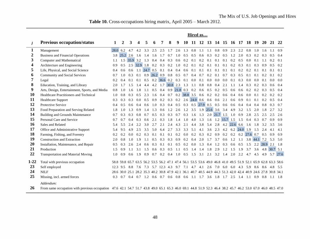
The Mix of U.S. Job Openings and Hires
48
Table 10. Cross-occupations hiring matrix, April 2005 – March 2012.
Hired as…
Previous occupation/status 1 2 3 4 5 6 7 8 9 10 11 12 13 14 15 16 17 18 19 20 21 22
1 Management 28.0 6.2 4.7 4.2 3.3 2.5 2.5 1.7 2.6 1.3 0.8 1.1 1.1 0.8 0.9 2.3 2.2 0.8 1.0 1.6 1.1 0.9
2 Business and Financial Operations 3.8 25.2 2.6 1.6 1.4 1.6 1.7 0.7 1.0 0.5 0.5 0.6 0.3 0.2 0.5 1.2 2.0 0.3 0.2 0.3 0.5 0.4
3 Computer and Mathematical 1.1 1.5 35.9 3.2 1.3 0.4 0.4 0.3 0.6 0.2 0.1 0.2 0.1 0.1 0.1 0.2 0.5 0.0 0.1 1.1 0.2 0.1
4 Architecture and Engineering 0.9 0.5 2.5 32.9 1.8 0.2 0.3 0.2 1.0 0.2 0.1 0.2 0.1 0.1 0.1 0.2 0.3 0.1 0.3 0.9 0.5 0.2
5 Life, Physical, and Social Science 0.4 0.6 0.6 1.1 24.7 0.5 0.1 0.4 0.4 0.6 0.1 0.1 0.1 0.1 0.1 0.1 0.2 0.2 0.1 0.1 0.1 0.1
6 Community and Social Services 0.7 1.0 0.3 0.1 0.9 26.2 0.9 0.8 0.5 0.7 0.4 0.7 0.2 0.1 0.7 0.3 0.5 0.1 0.1 0.2 0.1 0.2
7 Legal 0.2 0.4 0.1 0.1 0.5 0.2 36.6 0.2 0.3 0.1 0.0 0.1 0.0 0.0 0.0 0.1 0.3 0.0 0.0 0.1 0.0 0.0
8 Education, Training, and Library 2.0 1.7 1.5 1.4 4.4 4.2 1.7 30.8 2.3 1.3 1.1 0.8 0.8 0.4 2.1 1.1 1.4 0.3 0.2 0.3 0.6 0.4
9 Arts, Design, Entertainment, Sports, and Media 0.8 1.0 1.6 1.8 1.1 0.5 0.4 0.9 21.8 0.3 0.2 0.6 0.5 0.2 0.5 0.6 0.6 0.2 0.2 0.3 0.5 0.4
10 Healthcare Practitioners and Technical 1.0 0.8 0.3 0.5 2.3 1.6 0.4 0.7 0.2 38.8 3.5 0.6 0.2 0.2 0.6 0.4 0.6 0.0 0.1 0.2 0.2 0.2
11 Healthcare Support 0.3 0.3 0.3 0.0 0.5 0.9 0.2 0.3 0.2 2.6 24.0 0.6 0.6 0.6 2.1 0.6 0.9 0.1 0.1 0.2 0.5 0.4
12 Protective Service 0.4 0.5 0.6 0.4 0.6 1.0 0.3 0.4 0.5 0.3 0.5 27.9 0.5 0.5 0.6 0.6 0.4 0.4 0.4 0.8 0.3 0.7
13 Food Preparation and Serving Related 1.8 1.0 1.3 0.9 1.4 1.3 0.6 1.2 2.6 1.2 3.5 1.9 25.6 3.6 3.4 4.9 3.2 1.5 2.0 1.8 2.7 3.2
14 Building and Grounds Maintenance 0.7 0.3 0.3 0.8 0.7 0.5 0.3 0.3 0.7 0.3 1.6 1.3 2.0 21.7 1.5 1.0 0.9 2.8 2.5 2.5 2.5 2.6
15 Personal Care and Service 0.7 0.7 0.4 0.3 0.6 2.1 0.3 1.8 1.4 1.0 4.0 1.3 1.6 1.2 15.7 1.5 1.5 0.4 0.3 0.7 0.9 0.9
16 Sales and Related 5.4 5.5 2.4 2.2 3.0 2.7 2.1 2.4 4.3 2.1 4.4 3.8 5.4 2.8 4.2 22.6 6.6 1.6 1.8 3.2 3.5 3.6
17 Office and Administrative Support 5.4 9.5 4.9 2.5 3.5 5.0 6.4 2.7 3.3 3.3 5.1 4.1 3.6 2.3 4.2 6.2 24.0 1.9 1.5 2.4 4.1 4.1
18 Farming, Fishing, and Forestry 0.2 0.2 0.0 0.2 0.3 0.1 0.1 0.1 0.2 0.0 0.2 0.3 0.2 0.9 0.2 0.2 0.2 27.6 0.7 0.5 0.9 0.9
19 Construction and Extraction 2.0 0.8 1.0 1.9 1.1 0.5 0.3 0.3 0.9 0.2 0.4 2.0 1.7 3.7 0.6 1.2 1.1 3.8 44.1 7.2 5.3 5.0
20 Installation, Maintenance, and Repair 0.5 0.3 2.6 2.4 0.6 0.3 0.1 0.1 0.5 0.2 0.0 1.3 0.4 1.2 0.3 0.6 0.5 1.5 2.2 28.9 2.1 1.8
21 Production 1.5 0.9 1.1 3.1 1.5 0.6 0.3 0.5 1.1 0.5 1.4 1.4 1.8 2.9 1.2 1.5 1.9 3.7 3.6 4.8 30.7 5.1
22 Transportation and Material Moving 1.0 0.9 0.6 1.9 0.9 0.7 0.2 0.4 1.0 0.5 1.5 3.1 2.1 3.2 1.4 2.0 2.2 4.7 4.5 4.9 5.7 27.6
1-22 Total with previous occupation 58.8 59.8 65.7 63.5 56.2 53.5 56.2 47.1 47.4 56.1 53.5 53.6 49.0 46.8 41.0 49.5 51.9 52.1 65.9 62.8 63.3 58.6
23 Self employed 12.3 9.5 8.8 7.6 7.3 5.7 12.3 4.3 9.7 7.1 4.7 4.1 2.6 7.0 6.0 6.0 4.3 5.9 8.6 8.6 4.8 5.5
24 NILF 28.6 30.0 25.1 28.2 35.3 40.2 30.8 47.9 42.1 36.1 40.7 40.5 44.9 44.3 51.3 42.0 42.4 40.9 24.6 27.8 30.8 34.1
25 Missing, incl. armed forces 0.3 0.7 0.4 0.7 1.2 0.6 0.7 0.6 0.8 0.6 1.1 1.7 3.6 1.8 1.7 2.5 1.4 1.1 0.9 0.8 1.1 1.8
Addendum: 26 From same occupation with previous occupation 47.6 42.1 54.7 51.7 43.8 49.0 65.1 65.3 46.0 69.1 44.8 51.9 52.3 46.4 38.2 45.7 46.2 53.0 67.0 46.0 48.5 47.0
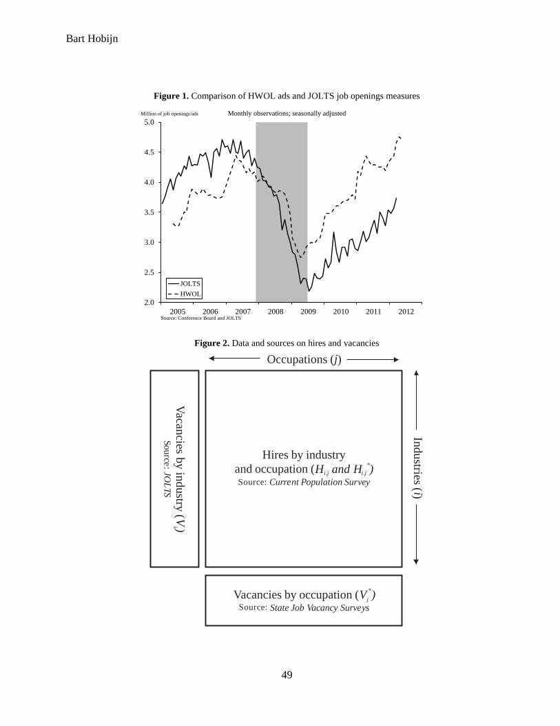
Bart Hobijn
49
Figure 1. Comparison of HWOL ads and JOLTS job openings measures
Figure 2. Data and sources on hires and vacancies
2.0
2.5
3.0
3.5
4.0
4.5
5.0
2005 2006 2007 2008 2009 2010 2011 2012
JOLTS
HWOL
Source: Conference Board and JOLTS
Monthly observations; seasonally adjustedMillion of job openings/ads
Occupations ( )j
Industries (
) i
Vacancies by occupation (V )j
*
Source: State Job Vacancy Surveys
Vacan
cies by in
dustry
( V)i
Source
: JOL
TS
Hires by industry
and occupation ( H )i.j
Source: Current Population Survey
H and i.j
*
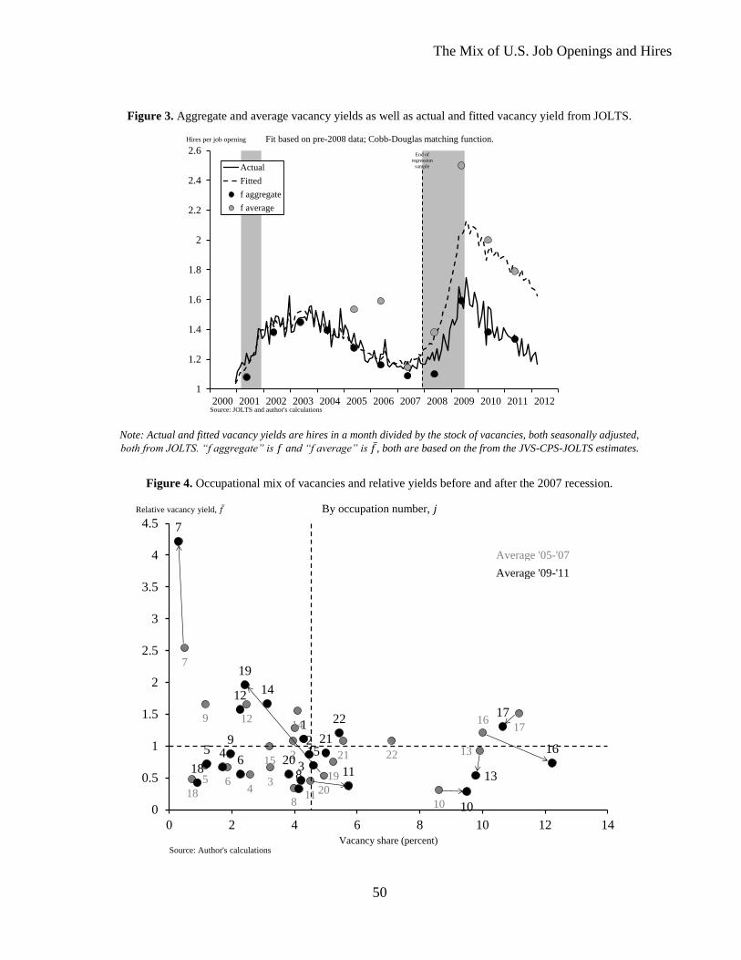
The Mix of U.S. Job Openings and Hires
50
Figure 3. Aggregate and average vacancy yields as well as actual and fitted vacancy yield from JOLTS.
Note: Actual and fitted vacancy yields are hires in a month divided by the stock of vacancies, both seasonally adjusted,
both from JOLTS. “f aggregate” is and “f average” is , both are based on the from the JVS-CPS-JOLTS estimates.
Figure 4. Occupational mix of vacancies and relative yields before and after the 2007 recession.
1
1.2
1.4
1.6
1.8
2
2.2
2.4
2.6
2000 2001 2002 2003 2004 2005 2006 2007 2008 2009 2010 2011 2012
Actual
Fitted
f aggregate
f average
Source: JOLTS and author's calculations
Fit based on pre-2008 data; Cobb-Douglas matching function.Hires per job opening
End of
regression
sample
12
34
5 6
7
8
9
1011
12
13
14
15
1617
18
19
20
21 22
1
2
345
6
7
8
9
10
11
12
13
14
15 16
17
18
19
20
21
22
0
0.5
1
1.5
2
2.5
3
3.5
4
4.5
0 2 4 6 8 10 12 14
Source: Author's calculations
By occupation number,
Vacancy share (percent)
Relative vacancy yield,
Average '09-'11
Average '05-'07
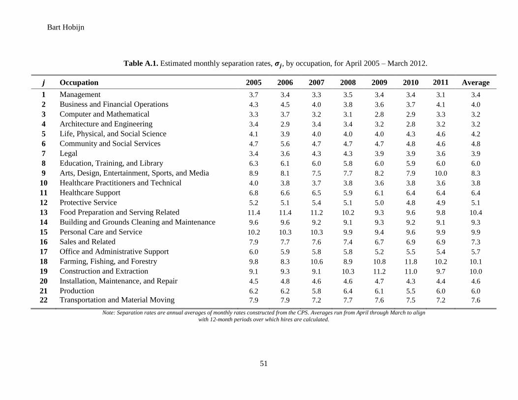
Bart Hobijn
51
Table A.1. Estimated monthly separation rates, , by occupation, for April 2005 – March 2012.
Occupation 2005 2006 2007 2008 2009 2010 2011 Average
1 Management 3.7 3.4 3.3 3.5 3.4 3.4 3.1 3.4
2 Business and Financial Operations 4.3 4.5 4.0 3.8 3.6 3.7 4.1 4.0
3 Computer and Mathematical 3.3 3.7 3.2 3.1 2.8 2.9 3.3 3.2
4 Architecture and Engineering 3.4 2.9 3.4 3.4 3.2 2.8 3.2 3.2
5 Life, Physical, and Social Science 4.1 3.9 4.0 4.0 4.0 4.3 4.6 4.2
6 Community and Social Services 4.7 5.6 4.7 4.7 4.7 4.8 4.6 4.8
7 Legal 3.4 3.6 4.3 4.3 3.9 3.9 3.6 3.9
8 Education, Training, and Library 6.3 6.1 6.0 5.8 6.0 5.9 6.0 6.0
9 Arts, Design, Entertainment, Sports, and Media 8.9 8.1 7.5 7.7 8.2 7.9 10.0 8.3
10 Healthcare Practitioners and Technical 4.0 3.8 3.7 3.8 3.6 3.8 3.6 3.8
11 Healthcare Support 6.8 6.6 6.5 5.9 6.1 6.4 6.4 6.4
12 Protective Service 5.2 5.1 5.4 5.1 5.0 4.8 4.9 5.1
13 Food Preparation and Serving Related 11.4 11.4 11.2 10.2 9.3 9.6 9.8 10.4
14 Building and Grounds Cleaning and Maintenance 9.6 9.6 9.2 9.1 9.3 9.2 9.1 9.3
15 Personal Care and Service 10.2 10.3 10.3 9.9 9.4 9.6 9.9 9.9
16 Sales and Related 7.9 7.7 7.6 7.4 6.7 6.9 6.9 7.3
17 Office and Administrative Support 6.0 5.9 5.8 5.8 5.2 5.5 5.4 5.7
18 Farming, Fishing, and Forestry 9.8 8.3 10.6 8.9 10.8 11.8 10.2 10.1
19 Construction and Extraction 9.1 9.3 9.1 10.3 11.2 11.0 9.7 10.0
20 Installation, Maintenance, and Repair 4.5 4.8 4.6 4.6 4.7 4.3 4.4 4.6
21 Production 6.2 6.2 5.8 6.4 6.1 5.5 6.0 6.0
22 Transportation and Material Moving 7.9 7.9 7.2 7.7 7.6 7.5 7.2 7.6
Note: Separation rates are annual averages of monthly rates constructed from the CPS. Averages run from April through March to align
with 12-month periods over which hires are calculated.