Embed Size (px)
Citation preview

The informational content of empirical measures of real interest rate andoutput gaps for the United Kingdom
Jens D J Larsen
and
Jack McKeown�
� Structural Economic and Monetary Assessment and Strategy Divisions, Mon-etary Analysis, Bank of England. E-mail: [email protected],[email protected].
This paper represents the views and analysis of the authors and should not be thought to representthose of the Bank of England or Monetary Policy Committee members. It has been prepared forthe BIS Autumn 2002 workshop on ‘Monetary policy in a changing environment’. It representswork-in-progress and is not to be qouted without explicit consent. We would like to thank, withoutimplicating, Luca Benati, who has been instrumental in generating the ideas that underlie thispaper, and who has provided extensive technical advice and assistance. We are grateful to PeterAndrews and participants at the BIS workshop for comments on this and earlier drafts. We thankRichard Geare and James Cookson for excellent research assistance.
This paper is work in progress and should not be cited or quoted from without the permission ofthe authors.

Contents
Abstract 3
Summary 4
1 Introduction 1
2 The model 5
3 Estimating the model parameters 8
4 Interpreting the gaps 13
5 Conclusion 23
Data 24
References 25
2

Abstract
In many economies, the monetary policy instrument is the level of short-term nominal interest
rates, but the monetary policy stance might be better characterised by the ex ante real interest rate
that this nominal rate implies, relative to some ‘neutral’ or ‘natural’ real rate of interest. In this
paper, the natural rate of interest and the real interest rate gap – the difference between the actual
and the ‘natural’ real rate of interest – is estimated by applying Kalman filtering techniques to a
small-scale macroeconomic model of the UK economy. In this model, the real interest rate gap,
the output gap and inflation are related via IS-curve and Phillips-curve relationships. The natural
rate of interest is defined as the level of (ex-ante) real interest rates that is consistent with an output
gap of zero, that is output at its ‘natural’ level, in the medium term. Based on these estimates, we
examine whether empirical measures of the real interest rate is a useful tool for policymakers -
does it contain additional information relative to the estimated output gap, and does the real rate
gap have leading indicator properties for the output gap and inflation? Are these gap estimates of
practical use in a policy setting? We find that the real rate gap has leading indicator properties for
both output gap and inflation. Importantly, these properties have varied considerably over time:
breaking our sample into four sub-samples, we find the leading indicator properties for both the
output and real rate gap to be substantially stronger for the sub-sample that comprises most of the
1980s. After the introduction of the inflation target, post 1992, the relationship between the real
interest rate gap and the output gap strengthens, but the leading indicator properties for inflation of
gaps diminishes, as we would expect given an inflation-targeting regime.
3

1 Introduction
The natural rate of interest is an object of interest to monetary policymakers: depending on the
exact definition of the concept, the natural rate may tell the policymaker exactly what the policy
rate should be (Woodford (1999) in his interpretation of Wicksell (1898)), or, combined with the
current policy rate and a measure of inflation expectations, indicate the current policy stance. In
this paper, we pursue the second interpretation by applying Kalman filtering techniques to UK
macroeconomic data to estimate jointly unemployment, output and real rate gaps, along with
expected inflation. The baseline model is a simple macro model where a positive real rate gap, the
difference between the expected short-term real interest rate and the natural rate, causes a negative
output gap, the difference between the actual and the natural level of output, which in turn is
related to the unemployment gap, the difference between the actual and the natural rate of
unemployment, via a variant of Okun’s law. Inflation expectations are formed according to a
generalised Phillips curve. (1) The natural real rate of interest, according to this definition, is the
real interest rate consistent with an output gap of zero in the medium term.
In principle, the model should be estimated jointly, but practical considerations force us to
estimate the model using a more restrictive approach, where we first estimate the model
parameters in blocks, and then jointly filter the data to obtain estimates for the gaps. (2)
Armed with these parameter estimates, we can identify the time-varying natural level of output,
the natural rate of unemployment and the natural rate of interest. We can then, in a straightforward
empirical exercise, assess the extent to which these measures are useful in a practical policy
setting. We first ask whether the estimated gaps are consistent with our priors about economic
history and policy developments—that is, do the estimates pass the ‘plausibility test’? To what
extent do the estimates provide meaningful insights on the developments in output, inflation and
interest rates? Second, we address the issue of which measure is most useful as an indicator of
future inflation or of ‘inflationary pressure’. While a policymaker will always want to consider
more than one indicator, it is nonetheless sensible to ask which gap is measured with greatest
(1) We use the terminology ‘natural’ and ‘gaps’ for output, real interest rates and unemployment. In principle, weshould always use inverted commas: there is nothing natural about the natural rate of interest, and, perhaps moreimportantly, there is a range of different definitions of what constitutes ‘natural’ and a ‘gap’. It is not suggested thatthe UK monetary authorities either did, or indeed should have, identified or responded to the particular concepts asdefined and estimated here.(2) We are still pursuing joint estimation of all model parameters.
1

precision, and which has the strongest indicator properties for future inflation. Thirdly, we ask
what we have we from imposing a model structure and using a maximum-likelihood estimation
technique. Would we be equally well off using simple univariate filtering techniques? A key point
of the exercise is to demonstrate that joint estimation of a model of this nature results in an
informational gain.
We find that the sample we study is characterised by substantial variation in the behaviour all of
the variables. In summary, the estimates of the real interest rate, the output and the unemployment
gap look plausible, and accord with our priors on the impact of economic events over time. We
find the estimated natural rate of interest to be negative towards the end of the 1970s, in line with
our ex-ante real interest rate estimates. But since the mid-1980s, both ex-ante and natural real
rates of interest have been positive. We interpret these estimates as being consistent with the
proposition that policy in the first period was relatively unresponsive to inflation, while policy in
the latter period has been more directly focused on controlling inflation. In terms of indicator
properties, we find that while both the output gap and the real interest rate gap have desirable
indicator properties for inflation over the sample as a whole, in line with the finding by Neiss and
Nelson (2001), this relationship has changed substantially over time. Breaking our sample into
four sub-samples, we find the leading indicator properties for both the output and real rate gap to
be substantially stronger for the sub-sample that comprises most of the 1980s. After the
introduction of the inflation target, post 1992, the relationship between the real interest rate gap
and the output gap strengthens, but the leading indicator properties of both for inflation
diminishes. We argue that this is consistent with the notion that nominal interest rates affect the
output gap via the real rate gap, and that policy is conducted with the aim of keeping expected
inflation constant and actual inflation close to target: in the language of policy rules, if policy were
implemented by changing the real interest rate gap, using short term nominal rates as the
instrument, in response to changes in the output gap and differences between expected inflation
and the target rate, then the deviation between the actual inflation rate and target rate will be close
to white noise: and, with a constant target rate, there will be no correlation between the real
interest rate and output gaps on the one hand, and the inflation on the other. (3)
The theoretical structure we impose on the data is deliberately relatively sparse. The reasoning
behind this choice is essentially one of simplicity and empirical robustness. Essentially, our model
(3) Please note footnote 1. There is no suggestion in this line of argument that UK monetary policy can be describedby or has followed such a rule.
2

consists of generalised IS and Phillips curves, with additional, largely statistical, assumptions
about the behaviour of the natural rate of interest, the natural level of output, and the natural rate
of unemployment: we impose relatively little structure, and ‘let the data speak’.
Laubach and Williams (2001) add further structure by assuming that the natural rate of interest is
related to trend growth of output, by reference to the ‘standard’ consumption Euler equation from
an optimal growth model. Svensson (2002), in his discussion of Laubach and Williams (2001) at
the AEA Annual Meetings, points out that even with such an additional assumption, the model
structure is still insufficient relative to the ‘minimum necessary model structure’ that is needed to
identify the natural rate of interest. Svensson argues that a fully specified dynamic general
equilibrium model, with sufficient structure to identify the real interest rate in a flexible price
economy, is the minimum necessary set of assumptions needed to produce a measure of the
natural rate of interest that can be given a structural interpretation.
Svensson’s interpretation of the concept of the natural rate of interest essentially coincides with
that of Woodford (1999) and Neiss and Nelson (2001). On this view, the natural rate of interest is
the real interest rate in an economy characterised by fully flexible prices, or, equivalently, the real
interest rate that equates actual output with potential output in a sticky price economy. By this
precise definition, it immediately follows that a dynamic general equilibrium structure is
necessary, but also sufficient: if a precise model has been specified, then there is no need to use a
statistical technique, such as the Kalman filter, to uncover latent variables, because these can be
computed directly from the model. And the resulting estimates can be treated as precise guides to
monetary policy: if optimal monetary policy entails setting actual output equal to potential, then
the natural rate of interested calculated from this model provides a direct read on the right level of
real interest rates.
At the other end of the modelling spectrum, where less or no structure is imposed, the ‘natural rate
of interest’ could be estimated by applying simple filtering techniques, such as linear detrending,
moving averages or Hodrick-Prescott filtering, of measures of the real interest rates, or simply as
long-term real interest rates on real assets, such as (forward) real interest rates implied by indexed
linked gilts in the United Kingdom or Treasury Inflation Protected Securities in the United States.
Using such an approach, no structural interpretations of the estimates are possible, and the
estimates cannot be construed as a direct guide to monetary policy.
3
We argue that a modelling approach in between these extremes should provide a useful tool for
monetary policy makers. Conceptually, the dynamic general equilibrium approach is desirable,
because it provides a direct read on optimal policy and a framework in which the movements in
the natural rate of interest can be given a structural interpretation. But in practice, constructing and
estimating a model that would be considered “credible” by policy makers, by virtue of desirable
features or some measure of fit with the data, is not a straightforward task. And solution
techniques and calibration techniques provide an additional obstacle: as Laubach and Williams
(2001) point out, models that rely on log-linear approximations around a non-stochastic
steady-state cannot be used to make inferences about low-frequency movements in the natural rate
of interest, because the long-run natural rate, by construction, is constant. The state of dynamic
general equilibrium modelling in the field of monetary economics is clearly progressing at a rapid
rate, with models such as Christiano, Eichenbaum and Evans (2001) and Smets and Wouters
(2002 providing clear improvements over the simplest baseline models, such as Cooley and
Hansen (1989), and policy models, such as those developed by some central banks, see e.g. Hunt,
Rose and Scott (2000), relying increasingly on structural features. On the other hand, a statistical
approach, with no economic model at all, is less useful in a policy context, because of the lack of
structural interpretation. If the natural rate measure derived from such a model has leading
indicator properties, are these permanent/structural features, or functions of the shocks hitting the
economy in a particular period?
An approach that includes some structure but allows for more empirical flexibility is useful when
assessing the real interest rate and the output gap in the United Kingdom. Over the sample we are
considering, the UK economy is characterised by a number of large shocks and structural changes,
so it is unlikely that a model without some allowance for changes in structural variables, such as
the level of the natural rate of interest, will provide an adequate tool when making an assessment
over time. By pursuing an approach that entails less structure than a dynamic general equilibrium
model, we, loosely speaking, lose the ability to provide a structural interpretation of the data, but
gain a better fitting explanation. The main focus of the paper is to provide a useful tool for
interpreting the data, and provide a feel for the extent to which the estimates of the output and real
rate gaps are useful, in the sense of having informational content, in a policy context.
With this approach, we are clearly not in a position to identify the estimated natural rate of interest
as the ‘optimal interest rate’ in the sense proposed by Woodford (1999). We follow Laubach and
4
Williams (2001) by interpreting the natural rate estimates as broadly measuring the intercept term
in a policy rule, but, in line with Woodford’s definition, doing so from the real side. We do not, at
this stage, model policy: that is nominal interest rates are taken as exogenously given, and, unlike
Plantier and Scrimgeour (2002), we do not attempt to characterise policy in the form of a policy
rule.
We have also estimated the natural rate of unemployment. But the natural rate of unemployment
plays only a small role in our analysis—we do not claim that these estimates are particularly
accurate or interesting in themselves, and acknowledge the fact that estimation of the natural rate
of unemployment is a difficult task in its own right. The estimated unemployment gap provides a
useful cross-check on the estimates of the real rate and the output gap.
The remainder of the paper is organised as follows. In Section 2, we outline the model, while
Section 3 discusses the estimation procedure and the parameter estimates. Section 4 discusses the
properties of our estimates and assess their usefulness is a practical setting. Section 5 concludes.
2 The model
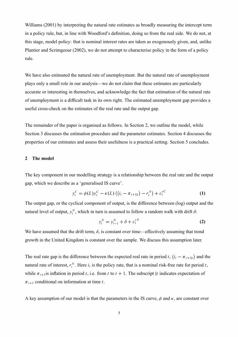
The key component in our modelling strategy is a relationship between the real rate and the output
gap, which we describe as a ‘generalised IS curve’.
yCt � ��L�yCt � ��L���it � � t�1�t
�� r Nt�� �
yCt (1)
The output gap, or the cyclical component of output, is the difference between (log) output and the
natural level of output, yNt , which in turn is assumed to follow a random walk with drift �:
yNt � yNt�1 � � � �yNt (2)
We have assumed that the drift term, �, is constant over time—effectively assuming that trend
growth in the United Kingdom is constant over the sample. We discuss this assumption later.
The real rate gap is the difference between the expected real rate in period t ,�it � � t�1�t
�and the
natural rate of interest, r Nt . Here it is the policy rate, that is a nominal risk-free rate for period t�
while � t�1is inflation in period t , i.e. from t to t � 1. The subscript �t indicates expectation of� t�1 conditional on information at time t .
A key assumption of our model is that the parameters in the IS curve, � and � , are constant over
5
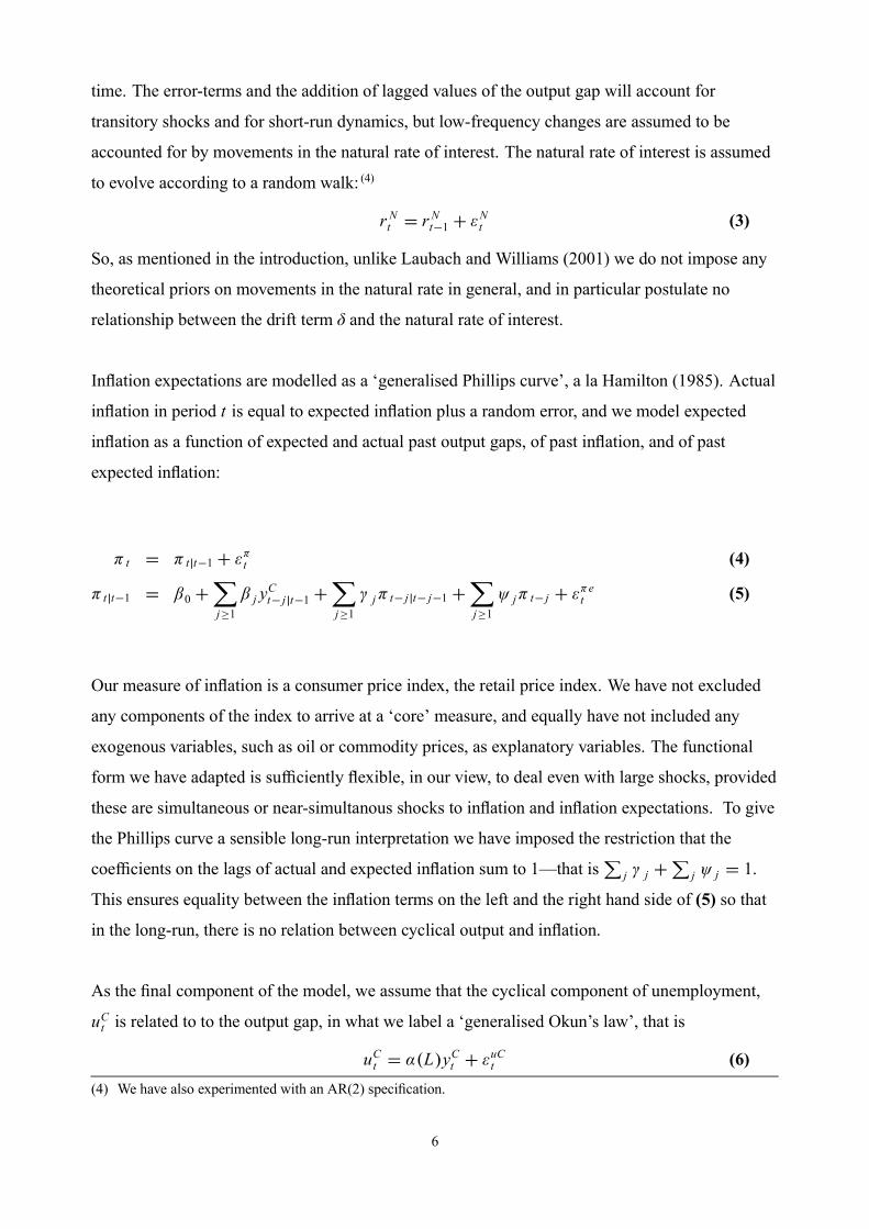
time. The error-terms and the addition of lagged values of the output gap will account for
transitory shocks and for short-run dynamics, but low-frequency changes are assumed to be
accounted for by movements in the natural rate of interest. The natural rate of interest is assumed
to evolve according to a random walk: (4)
r Nt � r Nt�1 � �Nt (3)
So, as mentioned in the introduction, unlike Laubach and Williams (2001) we do not impose any
theoretical priors on movements in the natural rate in general, and in particular postulate no
relationship between the drift term � and the natural rate of interest.
Inflation expectations are modelled as a ‘generalised Phillips curve’, a la Hamilton (1985). Actual
inflation in period t is equal to expected inflation plus a random error, and we model expected
inflation as a function of expected and actual past output gaps, of past inflation, and of past
expected inflation:
� t � � t�t�1 � ��t (4)
� t �t�1 � 0 ��
j�1 j yCt� j �t�1 �
�
j�1 j� t� j �t� j�1 �
�
j�1� j� t� j � ��et (5)
Our measure of inflation is a consumer price index, the retail price index. We have not excluded
any components of the index to arrive at a ‘core’ measure, and equally have not included any
exogenous variables, such as oil or commodity prices, as explanatory variables. The functional
form we have adapted is sufficiently flexible, in our view, to deal even with large shocks, provided
these are simultaneous or near-simultanous shocks to inflation and inflation expectations. To give
the Phillips curve a sensible long-run interpretation we have imposed the restriction that the
coefficients on the lags of actual and expected inflation sum to 1—that is�
j j ��
j � j � 1.This ensures equality between the inflation terms on the left and the right hand side of (5) so that
in the long-run, there is no relation between cyclical output and inflation.
As the final component of the model, we assume that the cyclical component of unemployment,
uCt is related to to the output gap, in what we label a ‘generalised Okun’s law’, that is
uCt � ��L�yCt � �uCt (6)(4) We have also experimented with an AR(2) specification.
6
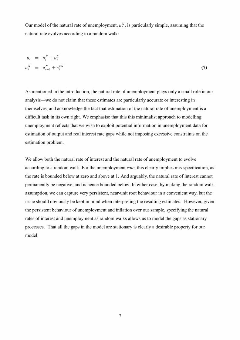
Our model of the natural rate of unemployment, uNt , is particularly simple, assuming that the
natural rate evolves according to a random walk:
ut � uNt � uCtuNt � uNt�1 � �uNt (7)
As mentioned in the introduction, the natural rate of unemployment plays only a small role in our
analysis—we do not claim that these estimates are particularly accurate or interesting in
themselves, and acknowledge the fact that estimation of the natural rate of unemployment is a
difficult task in its own right. We emphasise that this this minimalist approach to modelling
unemployment reflects that we wish to exploit potential information in unemployment data for
estimation of output and real interest rate gaps while not imposing excessive constraints on the
estimation problem.
We allow both the natural rate of interest and the natural rate of unemployment to evolve
according to a random walk. For the unemployment rate, this clearly implies mis-specification, as
the rate is bounded below at zero and above at 1. And arguably, the natural rate of interest cannot
permanently be negative, and is hence bounded below. In either case, by making the random walk
assumption, we can capture very persistent, near-unit root behaviour in a convenient way, but the
issue should obviously be kept in mind when interpreting the resulting estimates. However, given
the persistent behaviour of unemployment and inflation over our sample, specifying the natural
rates of interest and unemployment as random walks allows us to model the gaps as stationary
processes. That all the gaps in the model are stationary is clearly a desirable property for our
model.
7
3 Estimating the model parameters
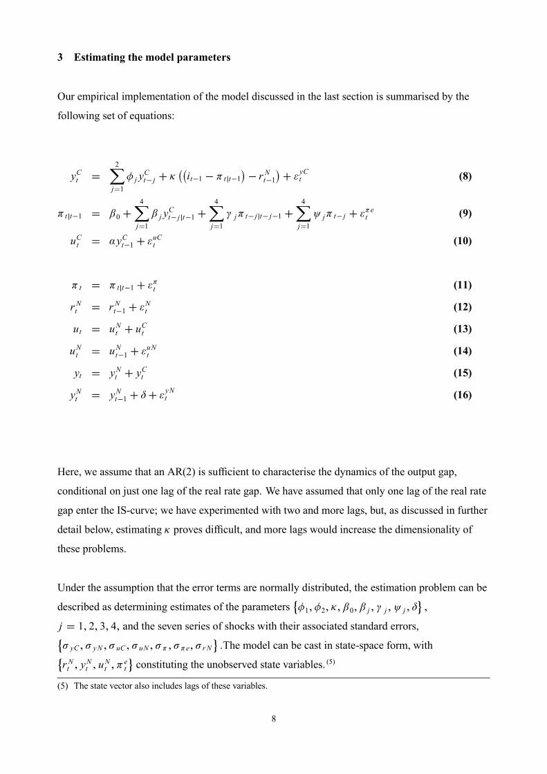
Our empirical implementation of the model discussed in the last section is summarised by the
following set of equations:
yCt �2�
j�1� j yCt� j � �
��it�1 � � t �t�1
�� r Nt�1�� �
yCt (8)
� t �t�1 � 0 �4�
j�1 j yCt� j �t�1 �
4�
j�1 j� t� j �t� j�1 �
4�
j�1� j� t� j � ��et (9)
uCt � �yCt�1 � �uCt (10)
� t � � t�t�1 � ��t (11)
r Nt � r Nt�1 � �Nt (12)
ut � uNt � uCt (13)
uNt � uNt�1 � �uNt (14)
yt � yNt � yCt (15)
yNt � yNt�1 � � � �yNt (16)
Here, we assume that an AR(2) is sufficient to characterise the dynamics of the output gap,
conditional on just one lag of the real rate gap. We have assumed that only one lag of the real rate
gap enter the IS-curve; we have experimented with two and more lags, but, as discussed in further
detail below, estimating � proves difficult, and more lags would increase the dimensionality of
these problems.
Under the assumption that the error terms are normally distributed, the estimation problem can be
described as determining estimates of the parameters��1� �2� �� 0� j � j � � j � �
��
j � 1� 2� 3� 4� and the seven series of shocks with their associated standard errors,� yC� yN � uC� uN � � � �e� r N
��The model can be cast in state-space form, with
�r Nt � yNt � uNt � � et
�constituting the unobserved state variables. (5)
(5) The state vector also includes lags of these variables.
8

3.1 The block approach
In principle, this model can be estimated by maximum likelihood using standard Kalman filtering,
yielding parameter estimates and, by subsequent filtering, estimates of the unobserved variables.
In practice, this approach has proved unsuccessful on UK data: we cannot estimate the parameters
of the model by a system approach and get ‘sensible’ and interpretable estimates of the parameters
of the unobserved state variables. Our interpretation of this problem is partly one of
dimensionality, and partly one of the relatively poor fit of the IS curve to UK data, in particular a
problem of determining the parameter estimate of � . We discuss this issue in detail below. We
have tried to reduce the problem of dimensionality by reducing the number of parameters in the
Phillips curve: while this substantially improves the significance and precision of the parameter
estimates in the Phillips curve, it does not materially improve our ability to provide significant
estimates of ��
Having failed to obtain reasonable system-based maximum likelihood estimates, we proceed
instead by applying maximum likelihood techniques to blocks of the models. Having obtained
parameter estimates from this, we filter the model to obtain joint estimates of the natural rates and
levels and the standard errors of the associated shocks. In the following, we first discuss this block
approach before turning our attention to the joint filtering stage.
Because the model is a set of simultaneous equations with unobserved variables, we cannot
straightforwardly apply single equation techniques. We proceed by first obtaining initial estimates
of the output and unemployment gap, and then use these gaps to estimate the remaining model
parameters, conditional on these initial gap estimates. In practice, we do this by exploiting the
state-space representation of the Hodrick-Prescott filter, see e.g. Stock and Watson (1999), to
obtain initial estimates of the output and unemployment gaps. We replace the equations
characterising the natural rate of unemployment (14) and natural level of output (16) with the
following set of equations:
uNt � 2uNt�1 � uNt�2 � �uNt
yNt � 2yNt�1 � yNt�2 � �yNt (17)
9

while maintaining the assumption that uCt � �yCt � Furthermore, we assume that the signal-to-noise
ratio—that is, the ratio between the standard errors of the shocks to the natural and cyclical
components of output and unemployment—can be characterised by two constants, q1 and q2, so
that:
yN � �q1 yC � uN � �
q2 uC (18)
This in turn implies that
uC � � yC � uN � ��q2 yC (19)
so that for a fixed �q1� q2�, the problem reduces to estimating � and yC . In calibrating q1, the ratio
between the shock to natural and cyclical output, we follow Stock and Watson (1999) and set
q1 � 0�675�1000. Based on experimentation with various values we calibrate the second ratio asq2 � q1�10. (6)
From this first stage, we obtain a preliminary estimate of the output gap, which we label �yCt . Wethen proceed to estimate the parameters of the Phillips curve (9), that is
� j � j � � j � � � �e
�,
treating the output gap gap as an exogenous variable by replacing �yCt� j �t�1 with �yCt� j . From thisestimation procedure, we also obtain a series for expected inflation, �� et ,which we use in thesubsequent estimation of the IS curve, (8).
Table 1 presents a summary of all the parameter estimates obtained using our block estimation
approach. Starting with the output and unemployment block, we find that we obtain a negative
value for the Okun’s law coefficient, significantly less than zero and also greater than -1, according
reasonably with what we would expect for this relationship. The estimate of the standard error of
shocks to the output gap is 1.8% and statistically significant. This value is quite large, but this is
unsurprising given the nature of the multivariate HP-filter. The estimates of the Phillips curve
parameters are all insignificant, apart from the estimate of 3, the second lag of the output gap,
and � , the standard error of the shocks to actual inflation.
�Table 1 approximately here�
The insignificance of the parameter estimates is, at least in part, down to the number of lags we
(6) Whether these values are plausible is, lacking any firm metric, a matter of taste. But we note that the choice of q2only affects the natural level of unemployment and the estimated Okun’s coefficient, �, where the first gets morevolatile while the second increases in absolute size as q2 decreases. In the subsequent stages of the block approach,only the output gap plays a role, so the choice of the value of q2 does not affect these results substantially.
10

have allowed: testing down for significance, we can obtain a specification where all the parameters
are significant. A likliehood ratio test indiactes that this reduced model is superior to the full
model. We report these estimates in the third and fourth column of Table 1. With this specification
we find that the constant term is insignificantly different from zero, which accords with our
rational expectations specification. Reassuringly we also find that the output gap has a positive
impact on inflation, at one lag, as we expect from economic theory and also as we require for the
logic underlying our model. We use this reduced specification for the Phillips curve in estimating
(8).
As mentioned, estimating (8) conditional on �yCt and �� et proves difficult. Unlike typical results forthe US, see e.g. Watson (1986) or Kuttner (1994), the coefficient on the second lag of the output
gap, �2, is insignificant and poorly determined, and we cannot obtain significant estimates of � ,
the parameter that governs the sensitivity of the output gap with respect to the real interest rate
gap. The fact that �2 is insignificant and with large standard errors, is less worrying and accords
with findings that UK GDP growth is less persistent than is found for the United States, see e.g.
Holland and Scott (1998). But an insignificant estimate for � constitutes a problem in the sense
that it suggest no significant relationship between the output and real interest rate gap. As
mentioned, a more comprehensive lag structure provides no solution to the problem: we have
experimented with further lags, and have found that while we get more sizeable estimates, the
parameters remain insignificant, and tend to be off-setting numerically. The parameters may be
poorly determined for a whole host of reasons: even if there is a significant relationship between
the output and real rate gap, it may, for instance, be difficult to estimate if parameters are varying
over time. Our interpretation of the estimation results is that the likelihood function is so flat that
this key parameter is difficult to estimate, and instead we proceed by calibrating � carefully, and
subjecting the resulting series to sensitivity analysis.
The variability of the real interest rate is, at this stage of the estimation procedure, intimately
linked to �: we plot the relationship between � and the estimated standard deviation of the natural
rate of interest in Chart 1 (a). Conditional on an output gap series, �yCt , a lower value of � implies aless variability in the estimated natural rate of interest. Or, put in terms of the way we are
modelling the conditionality, if r Nt is highly time-varying, the real rate gap will tend be smaller
and less persistent. This implies that a larger � will be required to match the (at this stage given)
variation in �yCt . A natural lower bound for � is hence the highest value that implies an
11

(approximately) constant natural rate of interest. There is no natural upper bound for �: in
principle, the variability of the natural rate of interest could exceed that of the ex-ante real interest
rate, see e.g. Rotemberg and Woodford (1997). However, we restrict our attention to values of �
which imply a natural rate of interest that is less volatile than the ex ante real interest rate because
we find these estimates most plausible. So we focus on values of � � 0�35 or less, as shown inChart 1 (a) .
�Chart 1 approximately here�
As for the choice of a benchmark value, a well-determined estimate of r N , the standard error of
the shocks to the natural rate of interest, imposes tight limits on the appropriate choice of �: it is
only for vaules of � of 0.35 or greater that the standard error is significant at the ten percent level.
Chart 1 (b) plots the t-statistics for the estimates of r N as a function of � , and from the chart we
infer that it is only for values of � of .35 or greater that r N is significant. We settle on � � �35 as
benchmark, which in practice implies substantial variation in the natural rate of interest over the
sample, because this value meets both our criteria: the natural rate is less volatile than the ex-ante
real interest rate and r N can be estimated as significant at the 10 percent level. For values of �
significantly greater than .35, the natural rate of interest becomes very volatile, so for the purposes
of the sensitivity analysis, we also consider � � �35 an upper bound, and analyse the implications
of lower values of � .
We report the parameter estimates for three calibrations of �; � � 0�2� 0�275 and 0�35 in Table 2and show the corresponding estimates for the natural real interest rate in Chart 1, panel c). In each
of the three specifications we find a significantly positive value for the first lag of the output gap
and for the standard error of shocks to the IS curve. We are unable to estimate the second lag of
the output gap as significantly different from zero. The standard error of shocks to the IS curve is
estimated as about 0.9 in all three specifications. As discussed above the choice of � is crucial for
our being able to estimate the standard errors of the shocks to the natural real rate as being
significantly different from zero. With � � 0�35 we estimate the standard error of the shocks to thenatural real interest rate as 0.33, slightly smaller than our estimate for the standard error of shocks
to the IS curve and to actual and expected inflation.
�Table 2 approximately here�
12
Our preferred value for � is similar to values estimated in other papers. For example, Nelson and
Nikolov (2002) present an estimate for the IS slope coefficient of 0�36 for the United Kingdom,
obtained from an instrumental variable estimation of a similarly specified IS curve. There are a
number of estimates of the slope of the IS curve from US and euro-area studies, see e.g. Smets and
Wouters (2002) and Rudebusch and Svensson (1999). Notably estimates for the US and euro-area
are typically lower than our estimates, see e.g. the comparison in Nelson and Nikolov (2002). This
is consistent with the notion that in a relatively small, open economy, such as the United
Kingdom, the IS curve may be flatter due to net trade being more interest elastic than domestic
demand. (7) But, at this stage, we have no further substantial evidence to underpin this estimate.
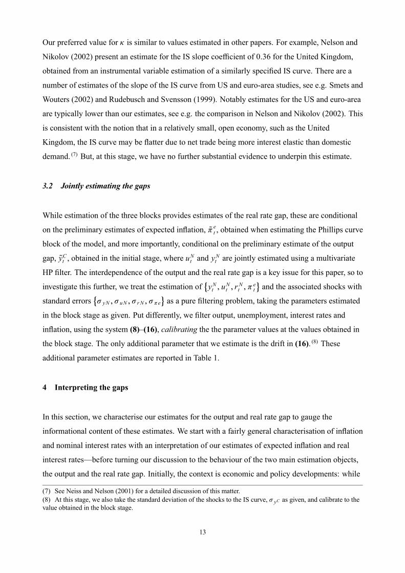
3.2 Jointly estimating the gaps
While estimation of the three blocks provides estimates of the real rate gap, these are conditional
on the preliminary estimates of expected inflation, �� et , obtained when estimating the Phillips curveblock of the model, and more importantly, conditional on the preliminary estimate of the output
gap, �yCt , obtained in the initial stage, where uNt and yNt are jointly estimated using a multivariateHP filter. The interdependence of the output and the real rate gap is a key issue for this paper, so to
investigate this further, we treat the estimation of�yNt � uNt � r Nt � � et
�and the associated shocks with
standard errors� yN � uN � r N � �e
�as a pure filtering problem, taking the parameters estimated
in the block stage as given. Put differently, we filter output, unemployment, interest rates and
inflation, using the system (8)–(16), calibrating the the parameter values at the values obtained in
the block stage. The only additional parameter that we estimate is the drift in (16). (8) These
additional parameter estimates are reported in Table 1.
4 Interpreting the gaps
In this section, we characterise our estimates for the output and real rate gap to gauge the
informational content of these estimates. We start with a fairly general characterisation of inflation
and nominal interest rates with an interpretation of our estimates of expected inflation and real
interest rates—before turning our discussion to the behaviour of the two main estimation objects,
the output and the real rate gap. Initially, the context is economic and policy developments: while
(7) See Neiss and Nelson (2001) for a detailed discussion of this matter.(8) At this stage, we also take the standard deviation of the shocks to the IS curve, � yC as given, and calibrate to thevalue obtained in the block stage.
13
a historic description of the estimates is not the key component of the exercise, it is nonetheless an
important ingredient because it provides an idea of the extent to which the estimates fit our prior
expectations and the consensus interpretation of economic events—that is, do the estimates pass
the plausibility test? Such a description is also helpful for the subsequent discussion of the
statistical properties of the various gaps: in this discussion, we focus on the extent to which the
real interest rate gap and output gap are useful leading indicators for inflation, and whether these
properties vary over time. We also discuss the extent to which our model approach implies an
informational gain relative to techniques, such as HP filtering, that rely less on assumptions about
the structure of the economy.
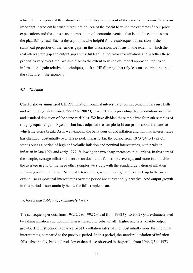
4.1 The data
Chart 2 shows annualised UK RPI inflation, nominal interest rates on three-month Treasury Bills
and real GDP growth from 1966 Q3 to 2002 Q3, with Table 3 providing the information on mean
and standard deviation of the same variables. We have divided the sample into four sub-samples of
roughly equal length—8 years—but have adjusted the sample to fit our priors about the dates at
which the series break. As is well-known, the behaviour of UK inflation and nominal interest rates
has changed substantially over this period: in particular, the period from 1973 Q4 to 1982 Q1
stands out as a period of high and volatile inflation and nominal interest rates, with peaks in
inflation in late 1974 and early 1979, following the two sharp increases in oil prices. In this part of
the sample, average inflation is more than double the full sample average, and more than double
the average in any of the three other samples we study, with the standard deviation of inflation
following a similar pattern. Nominal interest rates, while also high, did not pick up to the same
extent—so ex-post real interest rates over the period are substantially negative. And output growth
in this period is substantially below the full-sample mean.
�Chart 2 and Table 3 approximately here�
The subsequent periods, from 1982 Q2 to 1992 Q3 and from 1992 Q4 to 2002 Q3 are characterised
by falling inflation and nominal interest rates, and substantially higher and less volatile output
growth. The first period is characterised by inflation rates falling substantially more than nominal
interest rates, compared to the previous period. In this period, the standard deviation of inflation
falls substantially, back to levels lower than those observed in the period from 1966 Q3 to 1973
14

Q3, prior to the pick-up in inflation. The inflation targeting period, from 1992 Q4 to 2000 Q3, is
characterised by both low and stable inflation, with mean inflation of 2.5 percent with a standard
deviation of 1.48 percent, and low and stable nominal interest rates. Average output growth in this
period was higher than the level observed in the preceding period, and substantially less volatile.
4.2 Evaluating the estimates
Having characterised the data, we next turn to a discussion of our estimates of inflation
expectations and real interest rates, and subsequently of the natural rates and gaps.
Given our assumptions that link inflation expectations closely to actual inflation, it is unsurprising
to observe that expected inflation, whether the series estimated in the block approach or the series
from the subsequent joint filtering exercise, closely maps the behaviour of actual inflation. We
have reported the statistics of the estimated series in Table 4, together with the statistics for actual
inflation and mapped the series for expected inflation from the joint filtering stage against actual
inflation in Chart 3 (a) and compared it to the block estimate in Chart 3 (b). Both series pick out
the peaks in actual inflation in ’74 and ’79, and inflation expectations exhibit a sustained increase,
in line with actual, towards the end of the 1980s and the early 1990s, corresponding to large peaks
in aggregate demand, rapid rises in house prices and credit growth. And inflation expectations
have followed the subsequent disinflation and stability.
�Chart 3 and Table 4 approximately here�
In terms of model properties, we note that, as we would expect, expected inflation is less volatile
than actual inflation in all sub-samples, and expected inflation less ‘spiky’ than actual. The
estimated forecast errors from the block and joint filtering stage are closely related, with the
jointly filtered estimates being slightly less volatile than the block estimates. Both are stationary,
and the autocorrelation function, not shown here, indicates that the errors are white noise, as
implied by the model assumptions embedded in (11).
The ex-ante real interest rate estimates implied by these inflation expectations are shown in Chart
4 (a) and (b) and compared to ex-post rates. Table 5 give further details. Given the properties of
our estimates of expected inflation, it is unsurprising that ex-ante and ex-post real rates exhibit
15

similar behaviour. In terms of first moments, real interest rates are negative over the period from
1973 Q4 to 1982 Q1, but positive for all subsequent periods. In this period, real interest rates were
substantially more volatile than in subsequent periods, reflecting both the rise in inflation
expectations, but also the fact that the nominal rates used here, the 3 month Treasury Bill rate,
failed to respond strongly to the changes in expected inflation. Ex-ante real rates increased
strongly in the period from 1982 to 1992, reflecting the increased responsiveness of nominal rates
and the fall in expected inflation. Since the introduction of inflation targeting, real interest rates
have fallen from the high level observed in the 1980s, and are substantially less volatile than
observed in the previous periods.
�Chart 4 and Table 5 approximately here�
We characterise the estimated natural level of output and associated output gaps in Table 6 and
Chart 5. Because of the non-stationarity of output, we have characterised the natural level in terms
of growth rates. Both estimates of the natural level are less volatile than actual output growth, with
the estimate from the block stage being the least volatile. Given the nature of the model and the
techniques used for filtering out the unobserved level, this is, of course, unsurprising; the block
estimate is the least volatile, as this is, in essence, an HP-trend. Theoretically, there is no reason
why a smoothed measure of natural output should be preferred: indeed, the motivation for the
literature on estimation of New Keynesian Phillips curves, see e.g. Gali and Gertler (1999), is
motivated by the fact that smoothed or detrended output is a poor proxy for the natural level of
output.
�Chart 5 and Table 6 approximately here�
In output gap space, the difference between the two estimates is less striking: there is some
discrepancy in levels, but excluding the last five years of the sample, the correlation is substantial
at .68. The two series peak at the same times and at the same level, corresponding to the three
peaks in inflation discussed previously. The troughs occur at times of weak growth in aggregate
demand, following the oil price shocks in 1973 and 1979, and the period immediately after the
Gulf War in 1991. And negative output gaps are associated with falling inflation. These
observations, essentially, are consistent with our Phillips curve specification.
16

The divergence between the two gap estimates provides additional insights. Given the nature of
the block estimates, the output gap estimates from this stage are essentially independent of
inflation and interest rates. In the first part of the sample, up till the first spike in inflation, the
continued increase in inflation gives rise to a positive output gap when we allow for inflation
dependence, while the fall in inflation post 1981 has a negative impact on the estimate of the
output gap from the joint filtering stage. Neither of these effects are picked up by the block
estimates: the multivariate HP filter smooths out these effects on the output gap, because the
pick-up in output growth in these period was relatively gradual. Unemployment should affect both
estimates of the output gap—recall, that the block stage includes a joint filtering of the output and
unemployment—this does not provide any substantial help in explaining the difference, because
unemployment was increasing at the same time as inflation.
But from 1995 and onwards, the gaps have diverged, while inflation has remained low and stable:
the natural level of output in the jointly estimated stage is consistently lower than estimates from
the block stage. Part of this is down to the well-known problems with using HP filters towards the
end of the sample—the fact that we have used multivariate filtering does not change this issue, so
some divergence towards the end of the sample is expected. But it is possible that the constant
drift assumption plays a major part: in the joint filtering stage, we have prevented low-frequency
movement in the drift-term, �, while such moves will clearly be picked up by the HP filter.
Laubach and Williams (2001) take account of such movements by modelling low-frequency
movements in drift. (9)
Our estimates of the natural rate of interest and the associate real rate gaps are plotted in Chart 6
(a) and (c) and the associated standard statistics reported in Table 7. The divergence between the
natural rates is substantial, and though both natural rates are negative for sustained periods of
time, the period over which they are negative differs. And we note that as we observed with the
output gap, there is divergence towards the end of the sample—the higher output gap estimate for
the joint filtered estimates translate into an increase in the natural rate of interest. The level
implied by the joint stage towards the end of the sample seems, a priori, too high. However, given
the substantial time variation in our estimates of the natural real rate a better way to assess the
plausibility of the level of these estimates may be to look at the average level over a number of
years rather than at the level in any one period. Furthermore, we may wish to compare our
(9) We are continuing to study the implications of this assumption.
17
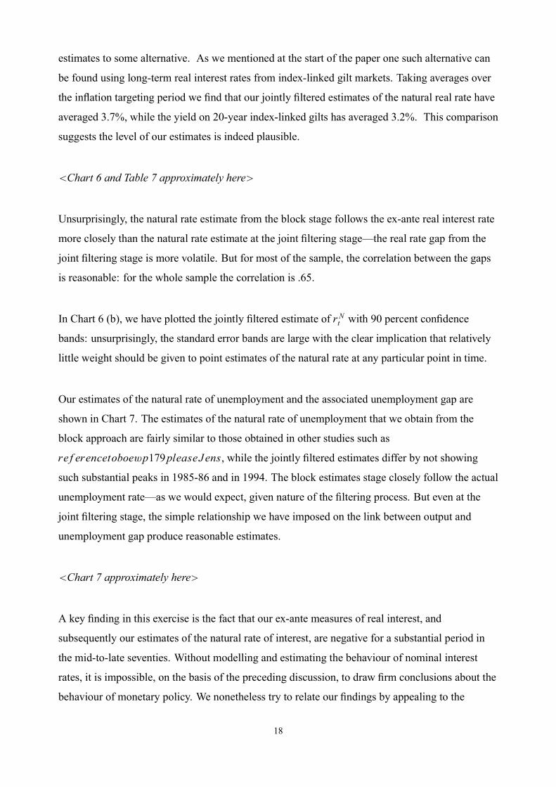
estimates to some alternative. As we mentioned at the start of the paper one such alternative can
be found using long-term real interest rates from index-linked gilt markets. Taking averages over
the inflation targeting period we find that our jointly filtered estimates of the natural real rate have
averaged 3.7%, while the yield on 20-year index-linked gilts has averaged 3.2%. This comparison
suggests the level of our estimates is indeed plausible.
�Chart 6 and Table 7 approximately here�
Unsurprisingly, the natural rate estimate from the block stage follows the ex-ante real interest rate
more closely than the natural rate estimate at the joint filtering stage—the real rate gap from the
joint filtering stage is more volatile. But for most of the sample, the correlation between the gaps
is reasonable: for the whole sample the correlation is .65.
In Chart 6 (b), we have plotted the jointly filtered estimate of r Nt with 90 percent confidence
bands: unsurprisingly, the standard error bands are large with the clear implication that relatively
little weight should be given to point estimates of the natural rate at any particular point in time.
Our estimates of the natural rate of unemployment and the associated unemployment gap are
shown in Chart 7. The estimates of the natural rate of unemployment that we obtain from the
block approach are fairly similar to those obtained in other studies such as
re f erencetoboe�p179pleaseJens, while the jointly filtered estimates differ by not showing
such substantial peaks in 1985-86 and in 1994. The block estimates stage closely follow the actual
unemployment rate—as we would expect, given nature of the filtering process. But even at the
joint filtering stage, the simple relationship we have imposed on the link between output and
unemployment gap produce reasonable estimates.
�Chart 7 approximately here�
A key finding in this exercise is the fact that our ex-ante measures of real interest, and
subsequently our estimates of the natural rate of interest, are negative for a substantial period in
the mid-to-late seventies. Without modelling and estimating the behaviour of nominal interest
rates, it is impossible, on the basis of the preceding discussion, to draw firm conclusions about the
behaviour of monetary policy. We nonetheless try to relate our findings by appealing to the
18
interpretation of the natural rate in this framework as ‘intercept in a policy rule’. For ease of
reference, take a simple policy rule such as that given below, where real interest rates will depend
on the natural rate of interest; the output gap; the difference between inflation and any inflation
target the monetary authority may be pursuing, given by �� and shocks �:
i � � e � rn � y �yc�� ��� � ���� � (20)
In the simplest version of this rule, the parameters are constant—but in principle, and in practice,
for this rule to be a useful description of the data, time-varying parameters are needed. We assume
that shocks are not (strongly) serially correlated, consistent with the interpretation low frequency
movements should be picked up by the natural rate of interest.
How can we interpret the persistently negative estimates of the r N? Actual ex-ante real interest
rates over this period were persistently negative, and to explain this using (20), we could appeal to
either changes in the response parameters y or �, a change in the target rate �� or policy
shocks. If the response parameters were constant, then persistently negative real interest rates
would require that the target rate would need to be increasing faster than a rapidly rising inflation
rate, or that policy shocks would need to be very persistent. So if policy in the 1970s were to be
characterised by a rule that allowed for changes in the natural rate of interest, then given the
negative ex-ante real interest rates, then it is unsurprising that the estimates of the natural rate of
interest are negative. But, as documented by Nelson and Nikolov (2002), policy in the 1970s was
not directed towards managing inflation—other policies, such as income policies and price
controls were used. Only in the 1980s was policy re-directed towards controlling inflation: in this
period, our estimates of the natural and ex-ante real interest rates turn positive. Even as inflation
peaked in 1990, the natural rate of interest remained positive. This broad characterisation is
consistent with the characterisation of ‘monetary policy neglect’ in Nelson and Nikolov (2002),
which suggests that policymakers in the 1970s did not regard monetary policy as a suitable tool
for controlling inflation: a policymaker that followed a policy rule, with a positive and constant
natural rate of interest in our interpretation, would have responded to the inflation shocks with
higher nominal interest rates. Nelson and Nikolov (2002) also present evidence on the ‘real-time
output gap mismeasurement’ hypothesis, advanced in a US context by Orphanides, see e.g.
Orphanides (2000) and Orphanides (2001). Based on this hypothesis both sets of authors suggest
that revisions to official data and estimates of the output gap played a substantial role in explaining
the lack of response of monetary policymakers. While we can provide no additional evidence on
the real time data issue—we use the latest vintage of UK National Accounts data throughout—we
19
will return to the issue of output gap mismeasurement in the next section.
4.3 Indicator properties/Informational gain
Having discussed the properties of the estimated time series, we now turn our attention to
assessing the use of the real interest rate and output gaps as forward-looking indicators for
inflation. In Chart 8, we consider the cross-correlation functions for the real interest rate gap, the
output gap and ex-ante real interest rates, together with the cross-correlation between the real rate
gap and output. In the left column are the cross-correlations from the jointly filtered stage, while
the right column shows the cross-correlations from the block stage. The chart is constructed so
that high correlations to the left of zero indicates leading indicator properties. The dotted lines
indicate 90 percent confidence bands.
�Chart 8 approximately here�
Looking at the entire sample, the model, whether estimated in blocks or by joint filtering, has
desirable indicator properties: both the real rate gap and the output gap lead inflation, with the
expected sign on the correlation being correct, and the real rate gap leads the output gap
significantly. The results from the jointly filtering stage, where we allow for more interaction
between the real interest rate and the output gap, are stronger. These results accord with the DGE
based findings in Neiss and Nelson (2001).
That said, there are, of course, some less desirable properties. First, the cross-correlation functions
for the real rate gap and inflation are virtually flat, with contemporaneous correlation being as high
as leads of the gap. And the ex-ante real interest rate itself is a stronger leading indicator than the
real rate gap: if we had assumed that the natural rate of interest were constant over the entire
sample, the real rate gap would have had stronger leading indicator properties.
But this performance over the entire sample masks substantial differences over sub-samples. Chart
9 provides the same cross-correlations as Chart 8, but broken into the sub-samples previously
discussed; in these charts, we have left out standard error bands to preserve clarity. Notice that the
number of observations in each sub-sample is fairly small—round 40—so although we offer fairly
clear-cut interpretations, it is clear that a (further) degree of caution should be exercised when
20

interpreting these statistics.
�Chart 9 approximately here�
Broadly characterised, we observe that
in all sub-samples, we estimate the expected negative (or insignificant) relationship between thereal interest rate gap and inflation. Similarly, the relationships between the output gap and
inflation, and between the output gap and the real rate gap, have the expected correlation.
the contemporaneous cross-correlation between the real interest rate gap and inflation isstrongest in the early sub-samples, running up to 1982, but the leading indicator properties are
strongest for the 1980s. The cross-correlation for the inflation targeting period is weaker than
for the 80s, particularly at longer lags and is insignificant at all leads and lags. We observe a
similar picture using the estimates from the block stage.
The picture for the output gap is similar in the sense that the correlations are stronger in the1980s than in both the later and earlier part of the sample.
But notably, for the joint filtering estimates, the relationship between the real interest rate gapand the output gap is strong both in the 1980s and the 1990s.
We interpret these results as follows. The relatively strong model performance in the 1982 to 1992
sample co-incides with a period we have characterised as one where inflation and interest rates are
more stable, and where ex-ante real interest rates are consistently positive: following the Nelson
and Nikolov interpretation, which we cannot substantiate further without modelling policy
behaviour explicitly, this is a period where monetary policy was directed towards controlling
inflation, and the links that we emphasise in this model more clearly understood.
But why do the relationships between the gaps and inflation weaken post 1992? We have
previously identified our assumption that the drift term � in (16) is assumed constant as a factor
that could change the dynamics of both the output gap and the real interest rate gap. Another is
that the ‘mix of shocks’ may have changed—this is an explanation on which we can offer limited
evidence given the relative sparse formulation of the model. A third is that a monetary policy
where interest rates respond strongly to predictions about future output gaps in order to stabilise
21
inflation would lead to inflation becoming less persistent and closer to white noise. If interest rates
affect inflation as suggested by this model, then such a policy would maintain or strengthen the
link between the real rate gap and the output gap—this is the means by which policy affects
inflation—and weaken the link between the gaps and inflation. Put another way, consider the
following manipulation of (20):
� � �� � 1�
��i � � e � rn�� y�yc�
�� e (21)
Assume that the target rate remains unchanged. If inflation persistently deviates from target, then
the difference between actual inflation and the target rate would be correlated with the real interest
rate and output gaps. But under under a credible inflation target expected inflation will be equal to
the target, and the deviation between actual inflation and the target will be white noise. In this
case, there will be no link between inflation and the gaps—but the gaps will continue to be
correlated, if the real rate gap responds to (expected) changes in the output gap. The
autocorrelation function for inflation, shown in Chart 10, is consistent with this interpretation:
inflation has become less persistent since 1992 than over the rest of the sample. (10)
�Chart 10 approximately here�
Clearly, any of the conclusions we have drawn on the basis of these estimates should be treated
with caution: for the latter comparisons, the samples are fairly small, and the standard errors large.
And, as stressed previously, we cannot draw firm conclusions about policy without modelling
policy explicitly.
Finally, in Chart 11, we compare the one-sided estimates with a simple (two-sided) HP-filtered
version of the real rate gap to assess the extent to which our modelling approach provides
additional information compared to an approach with no structure. We compare the one-sided
estimates with gap measures based on HP filtering of both the estimated ex-ante real interest and a
simple ex-post real rate. (11) In either case, the HP-filtered gaps have weaker indicator properties
than the model-based estimates.
�Chart 11 approximately here�
(10)Benati (2002) provides a much more comprehensive analysis of this issue.(11)Of course the latter is only available with a one period lag.
22
5 Conclusion
In this paper, we have assessed the usefulness of empirical estimates of the natural rate of interest
and the real rate gap, estimated in a model that allows for interaction between the real rate and the
output gap. We find that, despite empirical difficulties, these estimates are broadly plausible in
terms of accounting for the development of inflation, output growth and real interest rates in the
United Kingdom. Both output and real rate gaps have desirable indicator properties but that these
change substantially over time, in close relation to the dynamics of inflation.
While we think our estimates are useful in a policy context, we stress that we cannot interpret
these measures as an indication of the ‘correct’ level of the policy rate or of a definitive output gap.
The lack of model structure prevents such an interpretation—and as with any such estimates, there
is sufficient uncertainty around any point estimates to shy away from focusing on point estimates.
Our analysis clearly identifies that in periods with substantial structural change, an econometric
structure with constant parameters may struggle to provide interpretable estimates. An obvious,
but substantial, extension to our work is to consider time-varying parameters, particularly in the
relationship between the real interest rate and the output gap. Allowing for changes in this
relationship may substantially change the estimates of the natural rate of interest, particularly in
periods, such as the 1970s, that were characterised by a less coherent policy framework than the
current.
Given that we have focused on interpreting the estimated of the natural rate of interest as
‘intercept in a policy rule’, a natural next step is to estimate policy rules, as done by Laubach and
Williams (2001) for the United States and Plantier and Scrimgeour (2002) for New Zealand. Even
if, as is the case for both these countries and for the United Kingdom, policy is not conducted
according to a rule, a flexible rule—that allows for substantial variation both in response to gaps,
and allow for changes in targets guiding policy—would be useful way of describing policy.
23

Data
The data used in the paper are as follows. The output series is the quarterly growth rate of
seasonally adjusted UK GDP at constant market prices. The inflation data are seasonally adjusted
quarterly changes in UK RPI inflation. From 1992 and onwards, the unemployment data are LFS
unemployment. From 1979 to 1992, the annual LFS unemployment numbers have been
interpolated using the quarterly pattern in the Claimant Count and prior to this the annual numbers
from the OECD Labour Force Stats book have also been interpolated using the quarterly pattern in
the Claimant Count. The interest rate data are the three-month Treasury bill, where this has been
de-annualised to correspond to the return over three months.
24

References
Benati, L (2002), Investigating inflation persistence across monetary regimes. i: Empirical
evidence, Bank of England Mimeo.
Christiano, L, Eichenbaum, M, and Evans, M (2001), Nominal rigidities and the dynamic effects
of a shock to monetary policy, Federal Reserve Bank of Cleveland Working Paper, No. 07/01,
May.
Cooley, T F and Hansen, G D (1989) The inflation tax in a real business cycle model, American
Economic Review, pages 733–747.
Gali, J and Gertler, M (1999) Inflation dynamics: A structural econometric investigation, Journal
of Monetary Economics, Vol. 44, pages 195–222.
Hamilton, J D (1985) Uncovering financial markets expectations of inflation, Journal of Political
Economy, Vol. 93.
Holland, A and Scott, A (1998) The determinants of the UK business cycle, Economic Journal,
Vol. 108, pages 1067–92.
Hunt, B , Rose, D and Scott, A (2000) The core model of the Reserve Bank of New Zealand’s
forecasting and policy system, Economic Modelling, Vol. 17, pages 247–74.
Kuttner, K (1994) Estimating potential output as a latent variable, Journal of Business and
Economic Statistics, Vol. 12, No. 3, July, pages 361–68.
Laubach, T and Williams, J C (2001) Measuring the natural rate of interest, Board of Governors of
the Federal Reserve System, August.
Neiss, K and Nelson, E (2001) The real interest gap as an inflation indicator, Bank of England
Working Paper, No. 130.
25

Nelson, E and Nikolov, K (2002) Monetary policy and stagflation in the United Kingdom, Bank of
England Working Paper, No. 155.
Orphanides, A (2000) The quest for prosperity without inflation, European Central Bank, No. 15.
Orphanides, A (2001) Monetary policy rules, macroeconomic stability and inflation: A view from
the trenches, European Central Bank Working Paper, No. 115.
Plantier, L C and Scrimgeour, D (2002) Estimating a taylor rule for new zealand with a
time-varying neutral real rate, Reserve Bank of New Zealand Discussion Paper, No. 06.
Rotemberg, J J and Woodford, M (1997) An optimization-based econometric framework for the
evaluation of monetary policy, NBER Macroeconomics Annual, Vol. 12, pages 297–346.
Rudebusch, G D and Svensson, L E O (1999) Policy rules for inflation targeting, in Taylor, J B
(ed), Monetary Policy Rules, University of Chicago Press, pages 203–253.
Smets, F and Wouters, R (2002) An estimated stochastic dynamic general equilibrium model of
the euro area, European Central Bank, No. 171, August.
Stock, J and Watson, M (1999) Forecasting inflation, Journal of Monetary Economics, Vol. 44,
No. 2, pages 293–335.
Svensson, L E O (2002) Discussion of: Laubach and Williams: Measuring the natural interest
rate, Speaking notes prepared for presentation to American Economic Association’s Annual
Meeting 2002.
Watson, M (1986) Univariate detrending methods with stochastic trends, Journal of Monetary
Economics.
Wicksell, K (1958) The influence of the rate of interest on commodity prices, in Lindhal, E (ed),
Knut Wicksell, Selected Papers on Economic Theory, Harvard University Press.
26

Woodford, M (1999) A neo-Wicksellian framework for the analysis of monetary policy,
Manuscript, Princeton University.
27
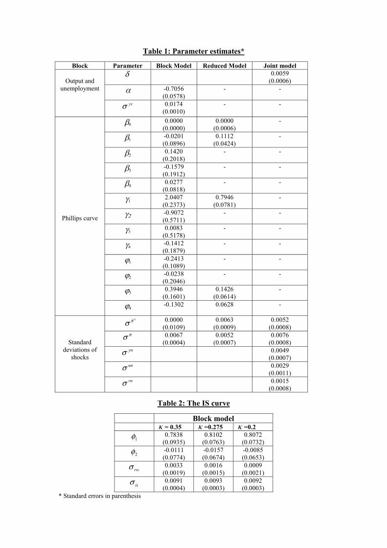
Table 1: Parameter estimates*
Block Parameter Block Model Reduced Model Joint modelδ 0.0059
(0.0006)α -0.7056
(0.0578)- -
Output andunemployment
ycσ 0.0174(0.0010)
- -
β00.0000
(0.0000)0.0000
(0.0006)-
β1-0.0201(0.0896)
0.1112(0.0424)
-
β20.1420
(0.2018)- -
β3-0.1579(0.1912)
- -
β40.0277
(0.0818)- -
γ12.0407
(0.2373)0.7946
(0.0781)-
γ2 -0.9072(0.5711)
- -
γ30.0083
(0.5178)- -
γ4-0.1412(0.1879)
- -
ϕ1-0.2413(0.1089)
- -
ϕ2-0.0238(0.2046)
- -
ϕ30.3946
(0.1601)0.1426
(0.0614)-
Phillips curve
ϕ4-0.1302 0.0628 -
eπσ 0.0000(0.0109)
0.0063(0.0009)
0.0052(0.0008)
πσ 0.0067(0.0004)
0.0052(0.0007)
0.0076(0.0008)
ynσ 0.0049(0.0007)
unσ 0.0029(0.0011)
Standarddeviations of
shocks
rnσ 0.0015(0.0008)
Table 2: The IS curve
Block modelκ = 0.35 κ =0.275 κ =0.2
1φ 0.7838(0.0935)
0.8102(0.0763)
0.8072(0.0732)
2φ -0.0111(0.0774)
-0.0157(0.0674)
-0.0085(0.0653)
rwσ 0.0033(0.0019)
0.0016(0.0015)
0.0009(0.0021)
isσ 0.0091(0.0004)
0.0093(0.0003)
0.0092(0.0003)
* Standard errors in parenthesis

Table 3: UK inflation, nominal interest rates and GDP growth
nominal interest ratemean st. dev mean st. dev mean st. dev
1966-2002 6.81 5.81 8.62 3.08 0.57 0.991966:3-1973:3 6.01 3.10 6.63 1.30 0.78 1.251973:4-1982:1 14.45 6.92 11.31 2.68 0.17 1.381982:2-1992:3 5.08 2.90 10.34 2.42 0.62 0.701992:4-2002:3 2.50 1.48 5.60 0.92 0.71 0.33
output growthactual inflation
Table 4: Actual and expected inflation
expected (joint) expected (block)mean st. dev mean st. dev mean st. dev
1966-2002 6.81 5.81 6.81 4.99 6.86 5.281966:3-1973:3 6.01 3.10 6.34 2.49 6.18 2.511973:4-1982:1 14.45 6.92 14.31 4.90 14.42 5.651982:2-1992:3 5.08 2.90 4.98 2.34 5.12 2.401992:4-2002:3 2.50 1.48 2.48 0.60 2.50 0.91
actual
Table 5: Real interest rates: ex-post and ex-ante
real rate (ex-post) real rate (joint) real rate (block)mean st. dev mean st. dev mean st. dev
1966-2002 1.81 4.84 1.81 4.03 1.80 4.241966:3-1973:3 0.63 2.99 0.29 2.35 0.52 2.461973:4-1982:1 -3.13 6.59 -3.00 4.97 -3.11 5.071982:2-1992:3 5.26 2.00 5.36 1.26 5.23 1.371992:4-2002:3 3.10 1.32 3.13 0.63 3.11 0.75
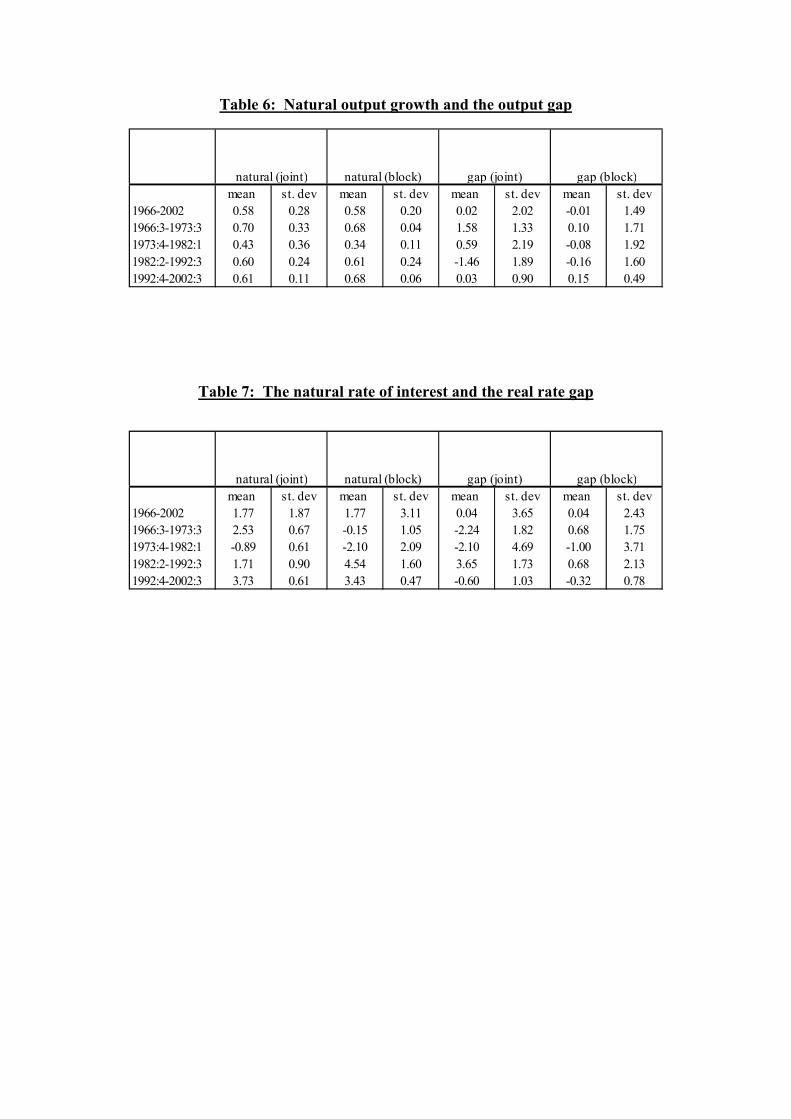
Table 6: Natural output growth and the output gap
mean st. dev mean st. dev mean st. dev mean st. dev1966-2002 0.58 0.28 0.58 0.20 0.02 2.02 -0.01 1.491966:3-1973:3 0.70 0.33 0.68 0.04 1.58 1.33 0.10 1.711973:4-1982:1 0.43 0.36 0.34 0.11 0.59 2.19 -0.08 1.921982:2-1992:3 0.60 0.24 0.61 0.24 -1.46 1.89 -0.16 1.601992:4-2002:3 0.61 0.11 0.68 0.06 0.03 0.90 0.15 0.49
natural (block)natural (joint) gap (joint) gap (block)
Table 7: The natural rate of interest and the real rate gap
mean st. dev mean st. dev mean st. dev mean st. dev1966-2002 1.77 1.87 1.77 3.11 0.04 3.65 0.04 2.431966:3-1973:3 2.53 0.67 -0.15 1.05 -2.24 1.82 0.68 1.751973:4-1982:1 -0.89 0.61 -2.10 2.09 -2.10 4.69 -1.00 3.711982:2-1992:3 1.71 0.90 4.54 1.60 3.65 1.73 0.68 2.131992:4-2002:3 3.73 0.61 3.43 0.47 -0.60 1.03 -0.32 0.78
gap (joint) gap (block)natural (joint) natural (block)
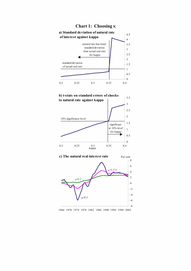
Chart 1: Choosing κ
0
0.5
1
1.5
2
2.5
3
3.5
4
4.5
0.2 0.25 0.3 0.35 0.4
a) Standard deviation of natural rate of interest against kappa
natural rate has lower standard deviation
than actual real rate for kappa
standard deviation of actual real rate
0
0.5
1
1.5
2
2.5
3
3.5
0.2 0.25 0.3 0.35 0.4
b) t-stats on standard errors of shocksto natural rate against kappa
kappa
significant at 10% level
for kappa
10% significance level
-8
-6
-4
-2
0
2
4
6
8
1966 1970 1974 1978 1982 1986 1990 1994 1998 2002
c) The natural real interest rate
κ=0.3
κ=0.275
κ=0.2
Per cent

Chart 2: UK Inflation, interest rates and GDP
-5
0
5
10
15
20
25
30
35
40
1966 1972 1978 1984 1990 1996 2002
a) UK inflation 1966:2002 Per cent
0
2
4
6
8
10
12
14
16
18
1966 1972 1978 1984 1990 1996 2002
b) UK nominal interest rates 1966:2002Per cent
-3
-2
-1
0
1
2
3
4
5
6
1966 1972 1978 1984 1990 1996 2002
c) UK quarterly GDP growth 1966:2002Per cent
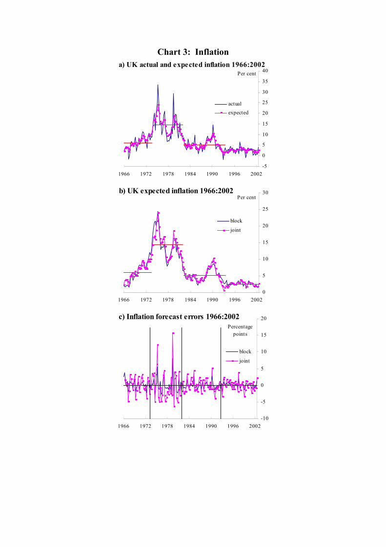
Chart 3: Inflation
-5
0
5
10
15
20
25
30
35
40
1966 1972 1978 1984 1990 1996 2002
actual
expected
a) UK actual and expected inflation 1966:2002Per cent
0
5
10
15
20
25
30
1966 1972 1978 1984 1990 1996 2002
block
joint
b) UK expected inflation 1966:2002Per cent
-10
-5
0
5
10
15
20
1966 1972 1978 1984 1990 1996 2002
block
joint
c) Inflation forecast errors 1966:2002Percentage
points
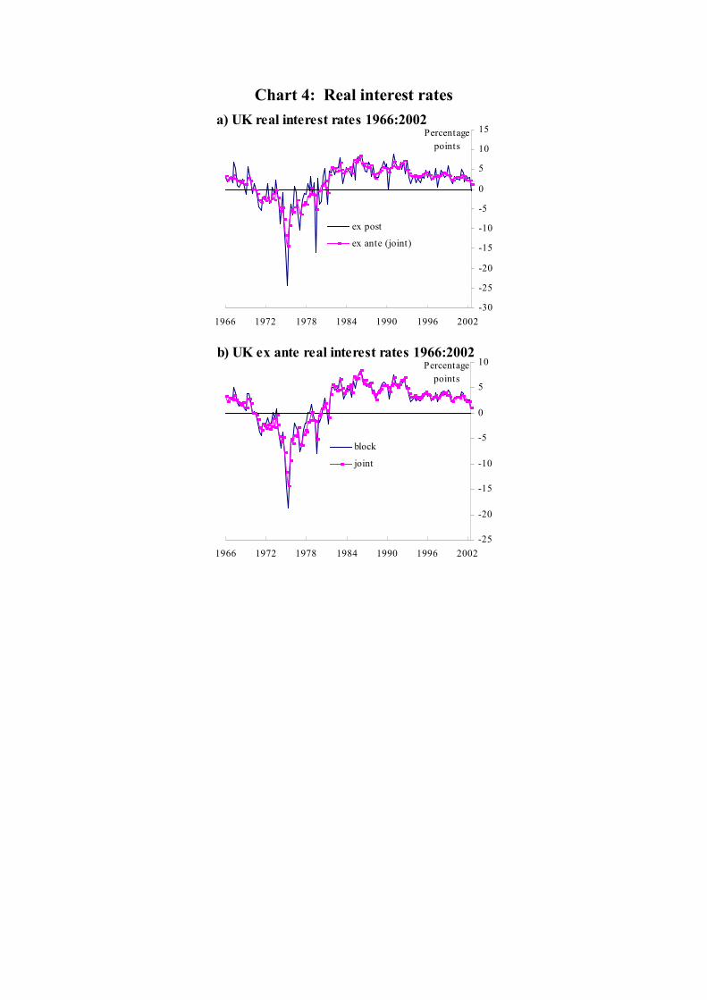
Chart 4: Real interest rates
-30
-25
-20
-15
-10
-5
0
5
10
15
1966 1972 1978 1984 1990 1996 2002
ex post
ex ante (joint)
a) UK real interest rates 1966:2002Percentage
points
-25
-20
-15
-10
-5
0
5
10
1966 1972 1978 1984 1990 1996 2002
block
joint
b) UK ex ante real interest rates 1966:2002Percentage
points

Chart 5: Output
-1
-0.5
0
0.5
1
1.5
2
1966 1970 1974 1978 1982 1986 1990 1994 1998 2002
a) UK natural output growth 1966:2002Per cent
block filteringjoint filtering
-6
-4
-2
0
2
4
6
1966 1970 1974 1978 1982 1986 1990 1994 1998 2002
b) UK output gap 1966:2002 Per cent
block filtering
joint filtering

Chart 6: Natural real interest rates
-8
-6
-4
-2
0
2
4
6
8
1966 1970 1974 1978 1982 1986 1990 1994 1998 2002
a) UK natural real interest rate: 1966:2002Per cent
Block filtering
Joint filtering
-8
-6
-4
-2
0
2
4
6
8
10
12
1966 1970 1974 1978 1982 1986 1990 1994 1998 2002
b) UK natural real interest rate: 1966:2002*Per cent
* Along with 90% confidence bands
-15
-10
-5
0
5
10
1966 1970 1974 1978 1982 1986 1990 1994 1998 2002
c) UK real rate gap 1966:2002 Per cent
block filtering
joint filtering

Chart 7: Unemployment
0
2
4
6
8
10
12
14
1966 1970 1974 1978 1982 1986 1990 1994 1998 2002
a) UK natural rate unemployment 1966:2002Per cent
joint filtering
block estimation
-4
-3
-2
-1
0
1
2
3
1966 1970 1974 1978 1982 1986 1990 1994 1998 2002
b) UK unemployment gap 1966:2002Per cent
block filtering
joint filtering
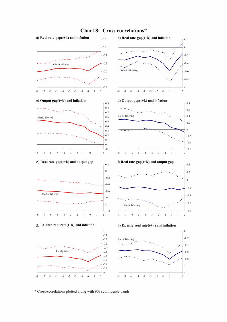
Chart 8: Cross correlations*
-0.9
-0.7
-0.5
-0.3
-0.1
0.1
0.3
-8 -7 -6 -5 -4 -3 -2 -1 0 1 2
a) Real rate gap(t+k) and inflation
Jointly filtered
-1
-0.8
-0.6
-0.4
-0.2
0
0.2
-8 -7 -6 -5 -4 -3 -2 -1 0 1 2
b) Real rate gap(t+k) and inflation
Block filtering
-0.1
0
0.1
0.2
0.3
0.4
0.5
0.6
0.7
0.8
0.9
-8 -7 -6 -5 -4 -3 -2 -1 0 1 2
c) Output gap(t+k) and inflation
Jointly filtered
-0.6
-0.4
-0.2
0
0.2
0.4
0.6
0.8
-8 -7 -6 -5 -4 -3 -2 -1 0 1 2
d) Output gap(t+k) and inflation
Block filtering
-1.2
-1
-0.8
-0.6
-0.4
-0.2
0
0.2
-8 -7 -6 -5 -4 -3 -2 -1 0 1 2
e) Real rate gap(t+k) and output gap
Jointly filtered
-0.8
-0.6
-0.4
-0.2
0
0.2
0.4
-8 -7 -6 -5 -4 -3 -2 -1 0 1 2
f) Real rate gap(t+k) and output gap
Block filtering
-1-0.9-0.8
-0.7-0.6-0.5-0.4-0.3-0.2-0.10
-8 -7 -6 -5 -4 -3 -2 -1 0 1 2
g) Ex ante real rate(t+k) and inflation
Jointly filtered
-1.2
-1
-0.8
-0.6
-0.4
-0.2
0
-8 -7 -6 -5 -4 -3 -2 -1 0 1 2
h) Ex ante real rate(t+k) and inflation
Block filtering
* Cross-correlations plotted along with 90% confidence bands
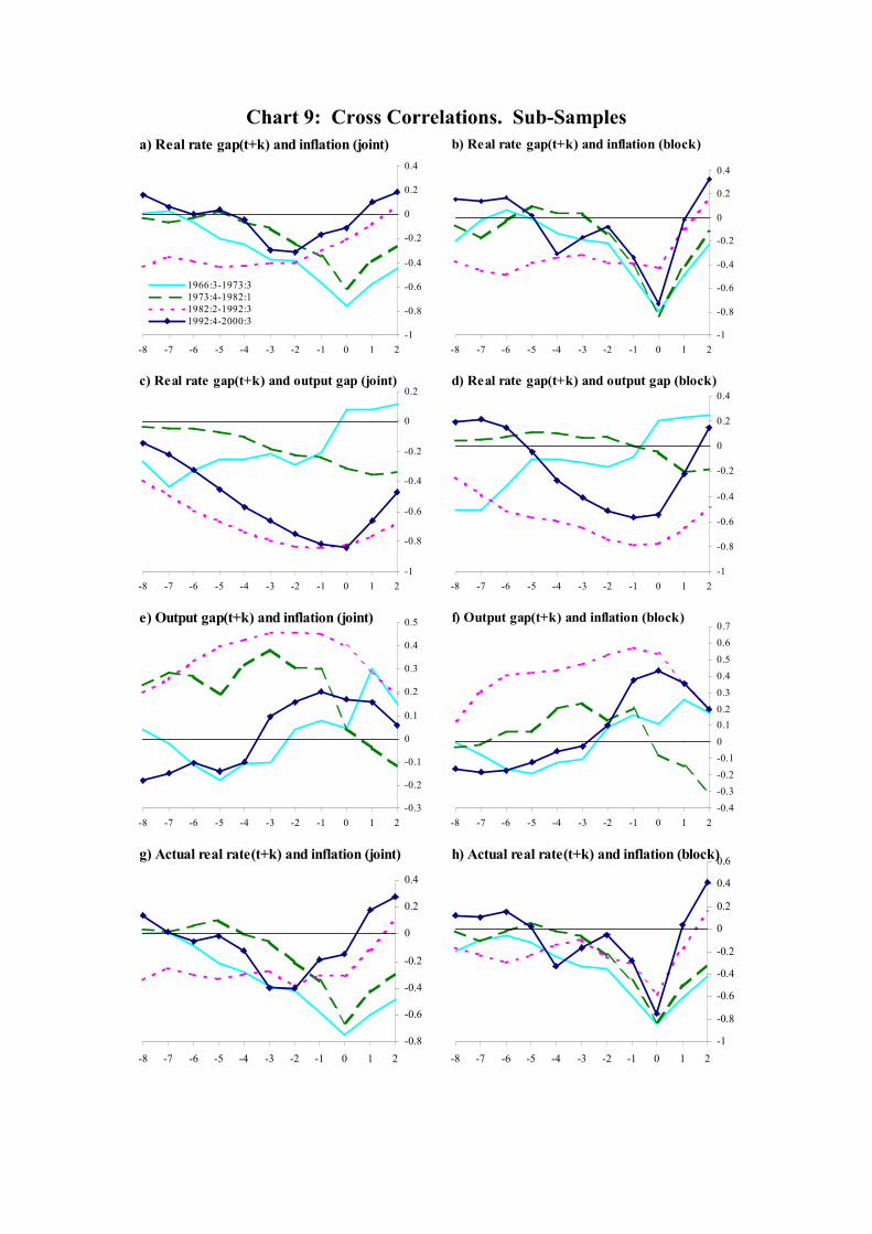
Chart 9: Cross Correlations. Sub-Samples
-1
-0.8
-0.6
-0.4
-0.2
0
0.2
0.4
-8 -7 -6 -5 -4 -3 -2 -1 0 1 2
1966:3-1973:31973:4-1982:11982:2-1992:31992:4-2000:3
a) Real rate gap(t+k) and inflation (joint)
-1
-0.8
-0.6
-0.4
-0.2
0
0.2
0.4
-8 -7 -6 -5 -4 -3 -2 -1 0 1 2
b) Real rate gap(t+k) and inflation (block)
-1
-0.8
-0.6
-0.4
-0.2
0
0.2
-8 -7 -6 -5 -4 -3 -2 -1 0 1 2
c) Real rate gap(t+k) and output gap (joint)
-1
-0.8
-0.6
-0.4
-0.2
0
0.2
0.4
-8 -7 -6 -5 -4 -3 -2 -1 0 1 2
d) Real rate gap(t+k) and output gap (block)
-0.3
-0.2
-0.1
0
0.1
0.2
0.3
0.4
0.5
-8 -7 -6 -5 -4 -3 -2 -1 0 1 2
e) Output gap(t+k) and inflation (joint)
-0.4-0.3-0.2
-0.10
0.10.20.3
0.40.5
0.60.7
-8 -7 -6 -5 -4 -3 -2 -1 0 1 2
f) Output gap(t+k) and inflation (block)
-0.8
-0.6
-0.4
-0.2
0
0.2
0.4
-8 -7 -6 -5 -4 -3 -2 -1 0 1 2
g) Actual real rate(t+k) and inflation (joint)
-1
-0.8
-0.6
-0.4
-0.2
0
0.2
0.4
0.6
-8 -7 -6 -5 -4 -3 -2 -1 0 1 2
h) Actual real rate(t+k) and inflation (block)

Chart 10: ACFs for inflation
-0.4
-0.2
0
0.2
0.4
0.6
0.8
1
-1 -2 -3 -4 -5 -6 -7 -8 -9 -10
a) ACF for inflation: 1966:3- 2002:3
-0.5-0.4-0.3-0.2-0.100.10.20.30.40.50.6
-1 -2 -3 -4 -5 -6 -7 -8 -9 -10
b) ACF for inflation: 1966:3-1973:3
-0.4
-0.3
-0.2
-0.1
0
0.1
0.2
0.3
0.4
0.5
-1 -2 -3 -4 -5 -6 -7 -8 -9 -10
c) ACF for inflation: 1973:4-1982:2
-0.5-0.4
-0.3-0.2-0.1
00.1
0.20.30.4
0.50.6
-1 -2 -3 -4 -5 -6 -7 -8 -9 -10
d) ACF for inflation: 1983:3-1992:3
-0.4
-0.3
-0.2
-0.1
0
0.1
0.2
0.3
0.4
-1 -2 -3 -4 -5 -6 -7 -8 -9 -10
e) ACF for inflation: 1992:4-2002:3

Chart 11: Cross correlations. One-sided estimates
-0.9
-0.7
-0.5
-0.3
-0.1
0.1
0.3
-8 -7 -6 -5 -4 -3 -2 -1 0 1 2
a) One-sided real rate gap(t+k) and inflation
Jointly filtered
-1
-0.8
-0.6
-0.4
-0.2
0
0.2
0.4
0.6
-8 -7 -6 -5 -4 -3 -2 -1 0 1 2
b) HP-filtered one-sided ex ante real rate (t+k)and inflation
-1
-0.8
-0.6
-0.4
-0.2
0
0.2
0.4
0.6
-8 -7 -6 -5 -4 -3 -2 -1 0 1 2
c) HP-filtered ex post real rate (t+k) and inflation