Embed Size (px)
Citation preview
THE INTRINSIC DIMENSIONALITY OF GRAPHS
ROBERT KRAUTHGAMER AND JAMES R. LEE
Abstract. We resolve the following conjecture raised by Levin together with Linial, London,
and Rabinovich [16]. For a graph G, let dim(G) be the smallest d such that G occurs as a (not
necessarily induced) subgraph of Zd∞, the infinite graph with vertex set Zd and an edge (u, v)
whenever ||u− v||∞ = 1. The growth rate of G, denoted ρG, is the minimum ρ such that every ball
of radius r > 1 in G contains at most rρ vertices. By simple volume arguments, dim(G) = Ω(ρG).
Levin conjectured that this lower bound is tight, i.e., that dim(G) = O(ρG) for every graph G.
Previously, it was unknown whether dim(G) could be bounded above by any function of ρG.
We show that a weaker form of Levin’s conjecture holds by proving that dim(G) = O(ρG log ρG)
for any graph G. We disprove, however, the specific bound of the conjecture and show that our
upper bound is tight by exhibiting graphs for which dim(G) = Ω(ρG log ρG). For several special
families of graphs (e.g., planar graphs), we salvage the strong form, showing that dim(G) = O(ρG).
Our results extend to a variant of the conjecture for finite-dimensional Euclidean spaces posed by
Linial [15] and independently by Benjamini and Schramm [22].
1. Introduction
The geometry of graphs, a fascinating area of combinatorics concerned with the geometric rep-
resentation of graphs, has found many algorithmic applications in recent years. A very fruitful
and actively studied line of research involves embedding the metric of a weighted graph into some
finite-dimensional real-normed space (see, for instance, the surveys [13] and [19, ch. 15]). In their
seminal paper [16], Linial, London, and Rabinovich were the first to fully realize the algorithmic im-
portance of low-distortion metric embeddings. However, their initial motivation was to understand
the relationship between the dimensionality of a graph and its combinatorial properties.
A notion of dimensionality is usually based on a particular way of embedding a graph into some
space that possesses an intrinsic dimension (e.g., a finite-dimensional Euclidean space). One then
defines the dimension of a graph to be the least dimension into which it can be embedded. Several
such notions have been extensively studied; see [18]. In [16], the authors wished to express the
Date: today.
2 ROBERT KRAUTHGAMER AND JAMES R. LEE
concept that graphs of “everywhere large diameter” should have low dimensionality. With the help
of Leonid Levin, this concept was was formalized as follows.
Let Zd∞ be the infinite graph with vertex set Zd and an edge (u, v) for two vertices u and v
whenever ||u− v||∞ = 1. For a graph G = (V,E), define dim(G) to be the smallest d such that G
occurs as a (not necessarily induced) subgraph of Zd∞.
For a pair of vertices u, v ∈ V , we define dG(u, v) to be the distance between u and v in the
shortest path metric on G. We denote by
B(v, r) = u ∈ V : dG(u, v) ≤ r
the closed ball of radius r in G centered at v, and define the growth rate of G to be
ρG = infρ : |B(v, r)| ≤ rρ for all v ∈ V and r > 1.
Equivalently, ρG = sup log |B(v,r)|log r : v ∈ V, r > 1. Notice that ρZd∞ = Θ(d), so by a simple counting
argument, we must have dim(G) = Ω(ρG). Levin, together with Linial, London, and Rabinovich
[16], conjectured that O(ρG) dimensions suffice.
Conjecture 1. For any graph G with growth rate ρG, G occurs as a (not necessarily induced)
subgraph of ZO(ρG)∞ . In other words, dim(G) = Θ(ρG).
In [16], it was shown that Conjecture 1 holds for the k-dimensional hypercube and the complete
binary tree, but nothing beyond these two special cases was known. Indeed, it was not known
whether dim(G) could be upper bounded by any function of ρG, even in the seemingly simpler
case when the graph is a tree. Linial [15] asked about a Euclidean analogue to this notion of
dimensionality.
Question 2. For a graph G = (V, E), what is the minimum dimension d, denoted dim2(G), such
that there exists a mapping γ : V → Rd with the following properties?
(1) ||γ(u)− γ(v)||2 ≥ 1 for all u 6= v ∈ V , and
(2) ||γ(u)− γ(v)||2 ≤ 2 for all (u, v) ∈ E.
Benjamini and Schramm [22] independently asked a similar question: Is it the case that, for
every infinite graph G with ρ(G) < ∞, we have dim2(G) < ∞? In what follows, we resolve all these
THE INTRINSIC DIMENSIONALITY OF GRAPHS 3
questions and give tight quantitative bounds. Linial remarked that the condition ||γ(u)−γ(v)||2 ≤ 2
is somewhat arbitrary; indeed, we will see that it can be replaced by ||γ(u) − γ(v)||2 ≤ C for any
fixed C >√
2 while affecting the value of dim2(G) by only a constant factor (see Section 6).
1.1. Results and techniques. In Section 2, we provide a self-contained proof of Levin’s conjecture
for trees. We first perform (two staggered) recursive decompositions of the tree. Each “level” of
the decomposition is responsible for pairs of vertices whose distance (in the tree) falls into a certain
range. For any single level we show that a map drawn from a particular distribution is a good
embedding of the level with high probability. If we embed each level independently and then
concatenate the resulting mappings, the dimension of the host lattice becomes too large. The
key technique, which completes the proof, is a method of handling all the levels using the same
coordinates. The solution involves a careful conservation of randomness between levels of the
induction (an idea which reappears throughout the paper). This result extends to graphs whose
induced simple cycles are of bounded length by known low-distortion embeddings of such graphs
into trees, due to [5, 6].
In Section 3, we give a lower bound on the dimension necessary to embed low-degree expander
graphs which shows that the strong form of Levin’s conjecture does not hold in general. In partic-
ular, we show that for a log n-degree expander G, dim(G) = Ω(ρG log ρG).
In Section 4, using different techniques, but many ideas from our proof for trees, we give a
general upper bound on dim(G) in terms of certain graph decompositions. In this setting, choosing
a good embedding for a level with high probability is more difficult; the approach we use is inspired
by a technique of [21] (which was used there to embed planar graphs into Euclidean space with
low distortion). Again, we must discover a delicate way of handling all the levels simultaneously.
In Section 4.4, we employ the decomposition of [14] (see also [10]), combined with the results of
Section 4, to prove the conjecture for any family of graphs which excludes a fixed minor (this
includes planar graphs, for instance).
In Section 5, we modify a probabilistic decomposition of [17, 3] for use with growth-restricted
graphs. Our modifications are two-fold. First, the parameters of our decomposition depend on ρ
(and not on n = |V | as in [17, 3]). This is essential to our application. Secondly, our decomposition
is local in the sense that events which are far apart (in G) are mutually independent. As a result,
4 ROBERT KRAUTHGAMER AND JAMES R. LEE
we are able to apply the Lovasz Local Lemma, yielding decompositions which, when combined with
the results of Section 4, give dim(G) = O(ρ3G) for any graph G.
To obtain a tight upper bound of dim(G) = O(ρG log ρG), we observe in Section 5.3 that the
many steps of our embedding can be essentially performed “at once,” removing the need to amplify
the individual probabilities at each step. Here, it is essential that every step of the embedding
process is “local” with respect to its “scale.”
Finally, in Section 6, it is shown that all our results for dim(G) hold also for Linial’s variant
dim2(G) [15], yielding a conclusive answer to Question 2, and positively resolving the question of
Benjamini and Schramm. This follows from a standard application of Chernoff-type tail bounds to
the random processes employed in previous sections.
1.2. Related work. Notions of dimensionality were perhaps first considered by Erdos, Harary,
and Tutte [8]. The geometric representations of graphs have been extensively studied in other
settings; see, for instance, the survey of Lovasz and Vesztergombi [18]. As mentioned before, the
related study of low-distortion metric embeddings has received increasing attention in recent years
(see the surveys [13, 19]).
Conjecture 1 is actually a dual of the bandwidth problem for graphs. The bandwidth problem
asks for the minimum stretch of any edge in an embedding of the graph into Z = Z1∞. Conjecture
1 asks for the minimum dimension needed to achieve a stretch of one (no stretch). Interestingly,
the density bound D = max |B(v,r)|2r (a one-dimensional analogue of the growth rate), which is a
straightforward lower bound on the bandwidth, is conjectured to be within a log |V | factor of the
bandwidth (this gap is met, for instance, by expanders). From [9], we know that the bandwidth and
density differ by only a polylog(|V |) factor. However, the techniques employed for the bandwidth
problem do not seem to help in resolving the dual question.
Imposing a growth restriction like |B(v, r)| ≤ rρ on a graph has many analogs in the analysis of
metric spaces, and in Riemannian geometry. For metric spaces, there are the notions of a doubling
metric and Ahlfors Q-regularity (see [12]). A metric space (X, d) is called doubling if it satisfies the
property that every ball in X can be covered by L balls of half the radius. Assouad showed that,
for any fixed 0 < ε < 1, the metric space (X, dε) (with distances raised to the power ε) embeds
into Rk with distortion D, where k and D depend only on L. This theorem is similar in spirit to a
number of the results presented here. Although Assouad’s methods are significantly different and
THE INTRINSIC DIMENSIONALITY OF GRAPHS 5
do not apply to Levin’s problem, the relationship is less than superficial; the techniques of Section
5 were used in [11] to obtain a new (quantitatively optimal) proof of Assouad’s theorem.
1.3. Preliminaries. For a point x = (x1, . . . , xd) ∈ Rd, we write ||x||2 = (∑d
i=1 |xi|2) 12 and
||x||∞ = maxdi=1 |xi|. For a graph G, we write V (G) and E(G) for the vertex and edge set of
G, respectively.
Definition 1.1. For a graph G = (V, E), a map ϕ : V → Zd is a contraction (or contractive) if
(u, v) ∈ E implies ||ϕ(u)−ϕ(v)||∞ ≤ 1. Furthermore, if ϕi is a finite set of mappings, we define
the direct sum, ϕ =⊕
i ϕi to be the mapping ϕ(u) = (ϕ1(u), ϕ2(u), . . .) (i.e., where coordinates are
concatenated).
Notice that if a map ϕ : V → Zd is both contractive and injective, then G occurs as a subgraph
of Zd∞, and in particular, dim(G) ≤ d. We can think of any such embedding ϕ as consisting of
d separate one-dimensional maps ϕ1, . . . , ϕd such that ϕ =⊕n
i=1 ϕi. The following simple lemma
will serve as our guide.
Lemma 1.2. Let G = (V,E) and ϕ =⊕d
i=1 ϕi where ϕi : V → Z, then the following are true.
(1) ϕ is a contraction ⇐⇒ every ϕi is a contraction.
(2) ϕ is injective ⇐⇒ for every pair u, v ∈ V , there exists some ϕi such that ϕi(u) 6= ϕi(v).
Unless otherwise stated, || · || = || · ||∞ and all logarithms are to the base 2.
2. Trees
In this section we show that every tree T with growth rate ρ occurs as a subgraph of Zd∞ with
d = O(ρ) by exhibiting a map ϕ : T → Zd that is both contractive and injective.
2.1. Embedding trees by random walks. In light of Lemma 1.2, it is natural to define a
distribution over random contractions and then argue that some such map must be injective.
Let T = (V, E) be a tree whose growth rate is at most ρ. Fix an arbitrary root r of T , and let
h be the height of T (so that V ⊆ B(r, h)). Define dT to be the shortest path metric on T and
let c > 0 be a sufficiently large constant to be determined later. Let T1, T2, . . . , Tcρ be cρ weighted
copies of T , where the weight of every edge in Ti is chosen independently and uniformly at random
6 ROBERT KRAUTHGAMER AND JAMES R. LEE
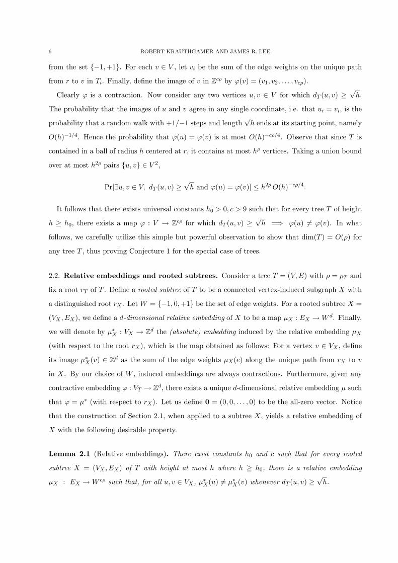
from the set −1,+1. For each v ∈ V , let vi be the sum of the edge weights on the unique path
from r to v in Ti. Finally, define the image of v in Zcρ by ϕ(v) = (v1, v2, . . . , vcρ).
Clearly ϕ is a contraction. Now consider any two vertices u, v ∈ V for which dT (u, v) ≥√
h.
The probability that the images of u and v agree in any single coordinate, i.e. that ui = vi, is the
probability that a random walk with +1/−1 steps and length√
h ends at its starting point, namely
O(h)−1/4. Hence the probability that ϕ(u) = ϕ(v) is at most O(h)−cρ/4. Observe that since T is
contained in a ball of radius h centered at r, it contains at most hρ vertices. Taking a union bound
over at most h2ρ pairs u, v ∈ V 2,
Pr[∃u, v ∈ V, dT (u, v) ≥√
h and ϕ(u) = ϕ(v)] ≤ h2ρ O(h)−cρ/4.
It follows that there exists universal constants h0 > 0, c > 9 such that for every tree T of height
h ≥ h0, there exists a map ϕ : V → Zcρ for which dT (u, v) ≥√
h =⇒ ϕ(u) 6= ϕ(v). In what
follows, we carefully utilize this simple but powerful observation to show that dim(T ) = O(ρ) for
any tree T , thus proving Conjecture 1 for the special case of trees.
2.2. Relative embeddings and rooted subtrees. Consider a tree T = (V, E) with ρ = ρT and
fix a root rT of T . Define a rooted subtree of T to be a connected vertex-induced subgraph X with
a distinguished root rX . Let W = −1, 0, +1 be the set of edge weights. For a rooted subtree X =
(VX , EX), we define a d-dimensional relative embedding of X to be a map µX : EX → W d. Finally,
we will denote by µ∗X : VX → Zd the (absolute) embedding induced by the relative embedding µX
(with respect to the root rX), which is the map obtained as follows: For a vertex v ∈ VX , define
its image µ∗X(v) ∈ Zd as the sum of the edge weights µX(e) along the unique path from rX to v
in X. By our choice of W , induced embeddings are always contractions. Furthermore, given any
contractive embedding ϕ : VT → Zd, there exists a unique d-dimensional relative embedding µ such
that ϕ = µ∗ (with respect to rX). Let us define 0 = (0, 0, . . . , 0) to be the all-zero vector. Notice
that the construction of Section 2.1, when applied to a subtree X, yields a relative embedding of
X with the following desirable property.
Lemma 2.1 (Relative embeddings). There exist constants h0 and c such that for every rooted
subtree X = (VX , EX) of T with height at most h where h ≥ h0, there is a relative embedding
µX : EX → W cρ such that, for all u, v ∈ VX , µ∗X(u) 6= µ∗X(v) whenever dT (u, v) ≥√
h.
THE INTRINSIC DIMENSIONALITY OF GRAPHS 7
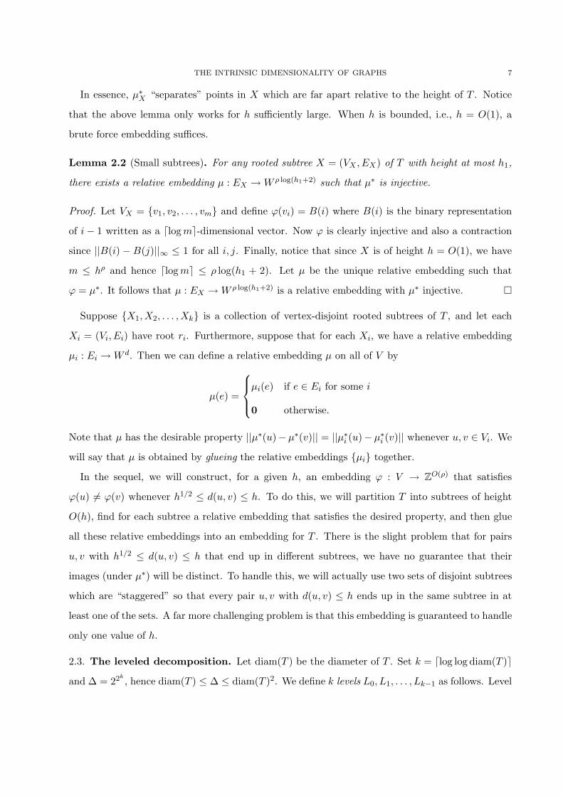
In essence, µ∗X “separates” points in X which are far apart relative to the height of T . Notice
that the above lemma only works for h sufficiently large. When h is bounded, i.e., h = O(1), a
brute force embedding suffices.
Lemma 2.2 (Small subtrees). For any rooted subtree X = (VX , EX) of T with height at most h1,
there exists a relative embedding µ : EX → W ρ log(h1+2) such that µ∗ is injective.
Proof. Let VX = v1, v2, . . . , vm and define ϕ(vi) = B(i) where B(i) is the binary representation
of i− 1 written as a dlog me-dimensional vector. Now ϕ is clearly injective and also a contraction
since ||B(i) − B(j)||∞ ≤ 1 for all i, j. Finally, notice that since X is of height h = O(1), we have
m ≤ hρ and hence dlog me ≤ ρ log(h1 + 2). Let µ be the unique relative embedding such that
ϕ = µ∗. It follows that µ : EX → W ρ log(h1+2) is a relative embedding with µ∗ injective. ¤
Suppose X1, X2, . . . , Xk is a collection of vertex-disjoint rooted subtrees of T , and let each
Xi = (Vi, Ei) have root ri. Furthermore, suppose that for each Xi, we have a relative embedding
µi : Ei → W d. Then we can define a relative embedding µ on all of V by
µ(e) =
µi(e) if e ∈ Ei for some i
0 otherwise.
Note that µ has the desirable property ||µ∗(u)− µ∗(v)|| = ||µ∗i (u)− µ∗i (v)|| whenever u, v ∈ Vi. We
will say that µ is obtained by glueing the relative embeddings µi together.
In the sequel, we will construct, for a given h, an embedding ϕ : V → ZO(ρ) that satisfies
ϕ(u) 6= ϕ(v) whenever h1/2 ≤ d(u, v) ≤ h. To do this, we will partition T into subtrees of height
O(h), find for each subtree a relative embedding that satisfies the desired property, and then glue
all these relative embeddings into an embedding for T . There is the slight problem that for pairs
u, v with h1/2 ≤ d(u, v) ≤ h that end up in different subtrees, we have no guarantee that their
images (under µ∗) will be distinct. To handle this, we will actually use two sets of disjoint subtrees
which are “staggered” so that every pair u, v with d(u, v) ≤ h ends up in the same subtree in at
least one of the sets. A far more challenging problem is that this embedding is guaranteed to handle
only one value of h.
2.3. The leveled decomposition. Let diam(T ) be the diameter of T . Set k = dlog log diam(T )eand ∆ = 22k
, hence diam(T ) ≤ ∆ ≤ diam(T )2. We define k levels L0, L1, . . . , Lk−1 as follows. Level
8 ROBERT KRAUTHGAMER AND JAMES R. LEE
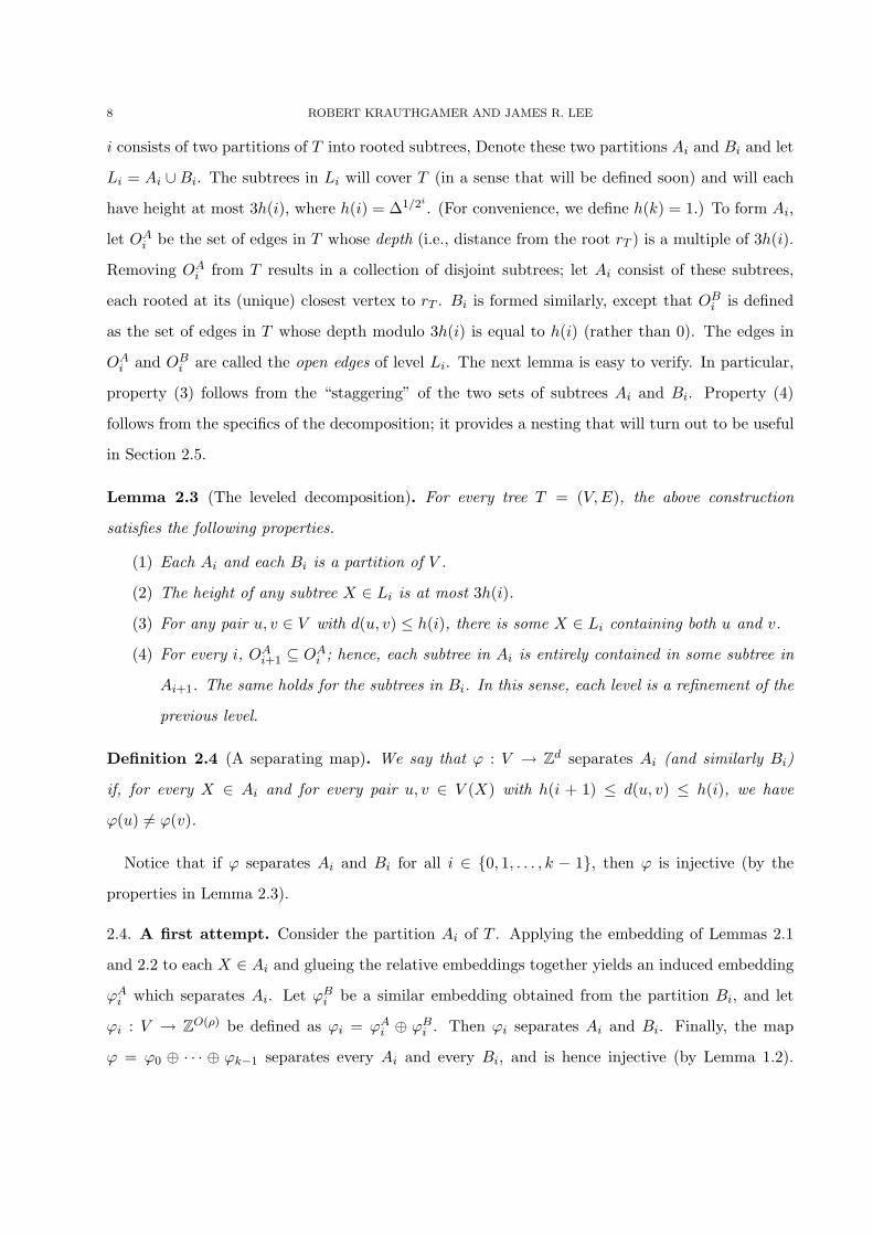
i consists of two partitions of T into rooted subtrees, Denote these two partitions Ai and Bi and let
Li = Ai ∪ Bi. The subtrees in Li will cover T (in a sense that will be defined soon) and will each
have height at most 3h(i), where h(i) = ∆1/2i. (For convenience, we define h(k) = 1.) To form Ai,
let OAi be the set of edges in T whose depth (i.e., distance from the root rT ) is a multiple of 3h(i).
Removing OAi from T results in a collection of disjoint subtrees; let Ai consist of these subtrees,
each rooted at its (unique) closest vertex to rT . Bi is formed similarly, except that OBi is defined
as the set of edges in T whose depth modulo 3h(i) is equal to h(i) (rather than 0). The edges in
OAi and OB
i are called the open edges of level Li. The next lemma is easy to verify. In particular,
property (3) follows from the “staggering” of the two sets of subtrees Ai and Bi. Property (4)
follows from the specifics of the decomposition; it provides a nesting that will turn out to be useful
in Section 2.5.
Lemma 2.3 (The leveled decomposition). For every tree T = (V,E), the above construction
satisfies the following properties.
(1) Each Ai and each Bi is a partition of V .
(2) The height of any subtree X ∈ Li is at most 3h(i).
(3) For any pair u, v ∈ V with d(u, v) ≤ h(i), there is some X ∈ Li containing both u and v.
(4) For every i, OAi+1 ⊆ OA
i ; hence, each subtree in Ai is entirely contained in some subtree in
Ai+1. The same holds for the subtrees in Bi. In this sense, each level is a refinement of the
previous level.
Definition 2.4 (A separating map). We say that ϕ : V → Zd separates Ai (and similarly Bi)
if, for every X ∈ Ai and for every pair u, v ∈ V (X) with h(i + 1) ≤ d(u, v) ≤ h(i), we have
ϕ(u) 6= ϕ(v).
Notice that if ϕ separates Ai and Bi for all i ∈ 0, 1, . . . , k − 1, then ϕ is injective (by the
properties in Lemma 2.3).
2.4. A first attempt. Consider the partition Ai of T . Applying the embedding of Lemmas 2.1
and 2.2 to each X ∈ Ai and glueing the relative embeddings together yields an induced embedding
ϕAi which separates Ai. Let ϕB
i be a similar embedding obtained from the partition Bi, and let
ϕi : V → ZO(ρ) be defined as ϕi = ϕAi ⊕ ϕB
i . Then ϕi separates Ai and Bi. Finally, the map
ϕ = ϕ0 ⊕ · · · ⊕ ϕk−1 separates every Ai and every Bi, and is hence injective (by Lemma 1.2).
THE INTRINSIC DIMENSIONALITY OF GRAPHS 9
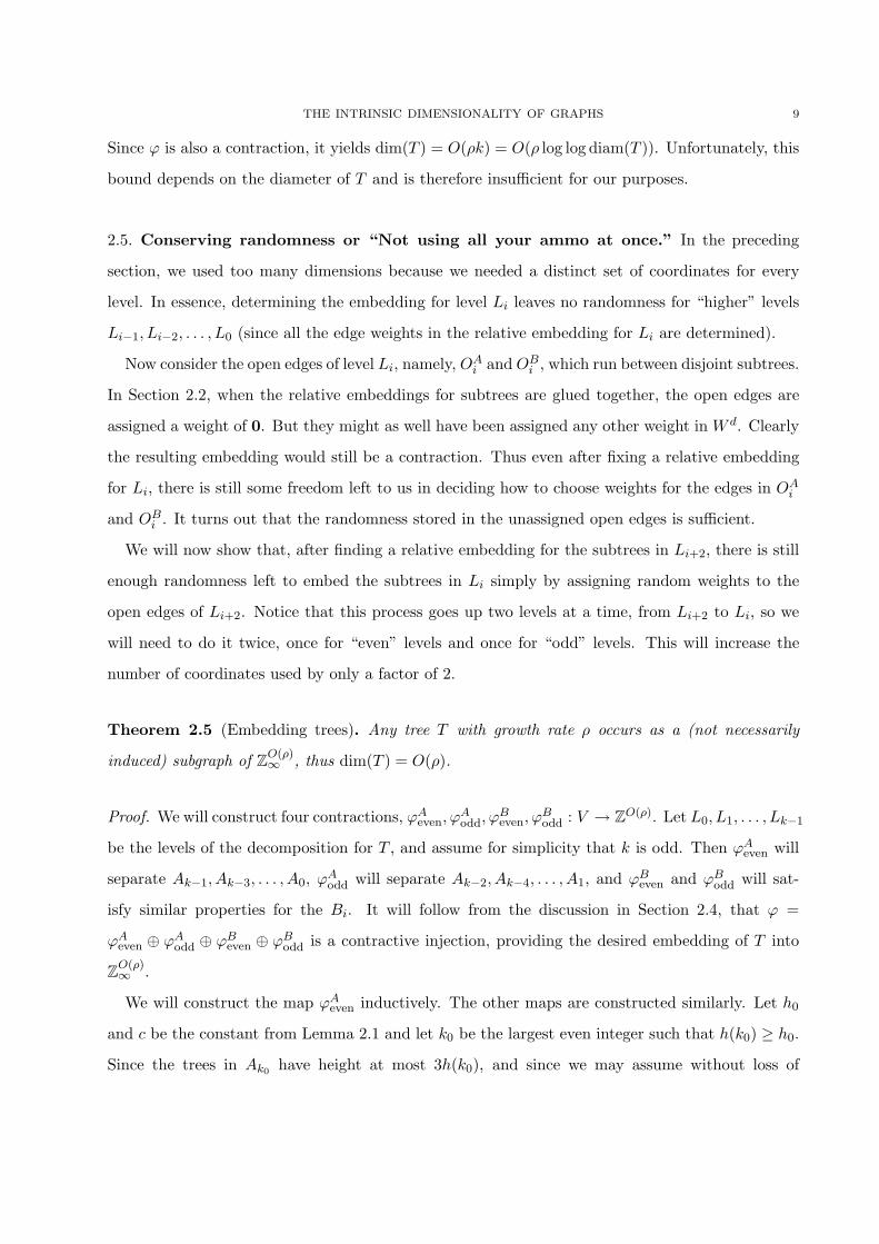
Since ϕ is also a contraction, it yields dim(T ) = O(ρk) = O(ρ log log diam(T )). Unfortunately, this
bound depends on the diameter of T and is therefore insufficient for our purposes.
2.5. Conserving randomness or “Not using all your ammo at once.” In the preceding
section, we used too many dimensions because we needed a distinct set of coordinates for every
level. In essence, determining the embedding for level Li leaves no randomness for “higher” levels
Li−1, Li−2, . . . , L0 (since all the edge weights in the relative embedding for Li are determined).
Now consider the open edges of level Li, namely, OAi and OB
i , which run between disjoint subtrees.
In Section 2.2, when the relative embeddings for subtrees are glued together, the open edges are
assigned a weight of 0. But they might as well have been assigned any other weight in W d. Clearly
the resulting embedding would still be a contraction. Thus even after fixing a relative embedding
for Li, there is still some freedom left to us in deciding how to choose weights for the edges in OAi
and OBi . It turns out that the randomness stored in the unassigned open edges is sufficient.
We will now show that, after finding a relative embedding for the subtrees in Li+2, there is still
enough randomness left to embed the subtrees in Li simply by assigning random weights to the
open edges of Li+2. Notice that this process goes up two levels at a time, from Li+2 to Li, so we
will need to do it twice, once for “even” levels and once for “odd” levels. This will increase the
number of coordinates used by only a factor of 2.
Theorem 2.5 (Embedding trees). Any tree T with growth rate ρ occurs as a (not necessarily
induced) subgraph of ZO(ρ)∞ , thus dim(T ) = O(ρ).
Proof. We will construct four contractions, ϕAeven, ϕ
Aodd, ϕ
Beven, ϕ
Bodd : V → ZO(ρ). Let L0, L1, . . . , Lk−1
be the levels of the decomposition for T , and assume for simplicity that k is odd. Then ϕAeven will
separate Ak−1, Ak−3, . . . , A0, ϕAodd will separate Ak−2, Ak−4, . . . , A1, and ϕB
even and ϕBodd will sat-
isfy similar properties for the Bi. It will follow from the discussion in Section 2.4, that ϕ =
ϕAeven ⊕ ϕA
odd ⊕ ϕBeven ⊕ ϕB
odd is a contractive injection, providing the desired embedding of T into
ZO(ρ)∞ .
We will construct the map ϕAeven inductively. The other maps are constructed similarly. Let h0
and c be the constant from Lemma 2.1 and let k0 be the largest even integer such that h(k0) ≥ h0.
Since the trees in Ak0 have height at most 3h(k0), and since we may assume without loss of
10 ROBERT KRAUTHGAMER AND JAMES R. LEE
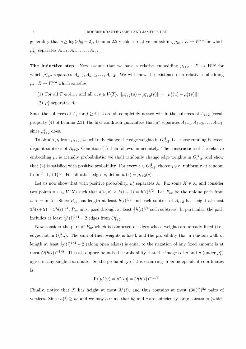
generality that c ≥ log(3h0 + 2), Lemma 2.2 yields a relative embedding µk0 : E → W cρ for which
µ∗k0separates Ak−1, Ak−3, . . . , Ak0 .
The inductive step. Now assume that we have a relative embedding µi+2 : E → W cρ for
which µ∗i+2 separates Ak−1, Ak−3, . . . , Ai+2. We will show the existence of a relative embedding
µi : E → W cρ which satisfies
(1) For all T ∈ Ai+2 and all u, v ∈ V (T ), ||µ∗i+2(u)− µ∗i+2(v)|| = ||µ∗i (u)− µ∗i (v)||;(2) µ∗i separates Ai.
Since the subtrees of Aj for j ≥ i + 2 are all completely nested within the subtrees of Ai+2 (recall
property (4) of Lemma 2.3), the first condition guarantees that µ∗i separates Ak−1, Ak−3, . . . , Ai+2,
since µ∗i+2 does.
To obtain µi from µi+2, we will only change the edge weights in OAi+2, i.e. those running between
disjoint subtrees of Ai+2. Condition (1) then follows immediately. The construction of the relative
embedding µi is actually probabilistic; we shall randomly change edge weights in OAi+2, and show
that (2) is satisfied with positive probability. For every e ∈ OAi+2, choose µi(e) uniformly at random
from −1, +1cρ. For all other edges e, define µi(e) = µi+2(e).
Let us now show that with positive probability, µ∗i separates Ai. Fix some X ∈ Ai and consider
two points u, v ∈ V (X) such that d(u, v) ≥ h(i + 1) = h(i)1/2. Let Puv be the unique path from
u to v in X. Since Puv has length at least h(i)1/2 and each subtree of Ai+2 has height at most
3h(i+2) = 3h(i)1/4, Puv must pass through at least 13h(i)1/4 such subtrees. In particular, the path
includes at least 13h(i)1/4 − 2 edges from OA
i+2.
Now consider the part of Puv which is composed of edges whose weights are already fixed (i.e.,
edges not in OAi+2). The sum of their weights is fixed, and the probability that a random walk of
length at least 13h(i)1/4 − 2 (along open edges) is equal to the negation of any fixed amount is at
most O(h(i))−1/8. This also upper bounds the probability that the images of u and v (under µ∗i )
agree in any single coordinate. So the probability of this occurring in cρ independent coordinates
is
Pr[µ∗i (u) = µ∗i (v)] = O(h(i))−cρ/8.
Finally, notice that X has height at most 3h(i), and thus contains at most (3h(i))2ρ pairs of
vertices. Since h(i) ≥ h0 and we may assume that h0 and c are sufficiently large constants (which
THE INTRINSIC DIMENSIONALITY OF GRAPHS 11
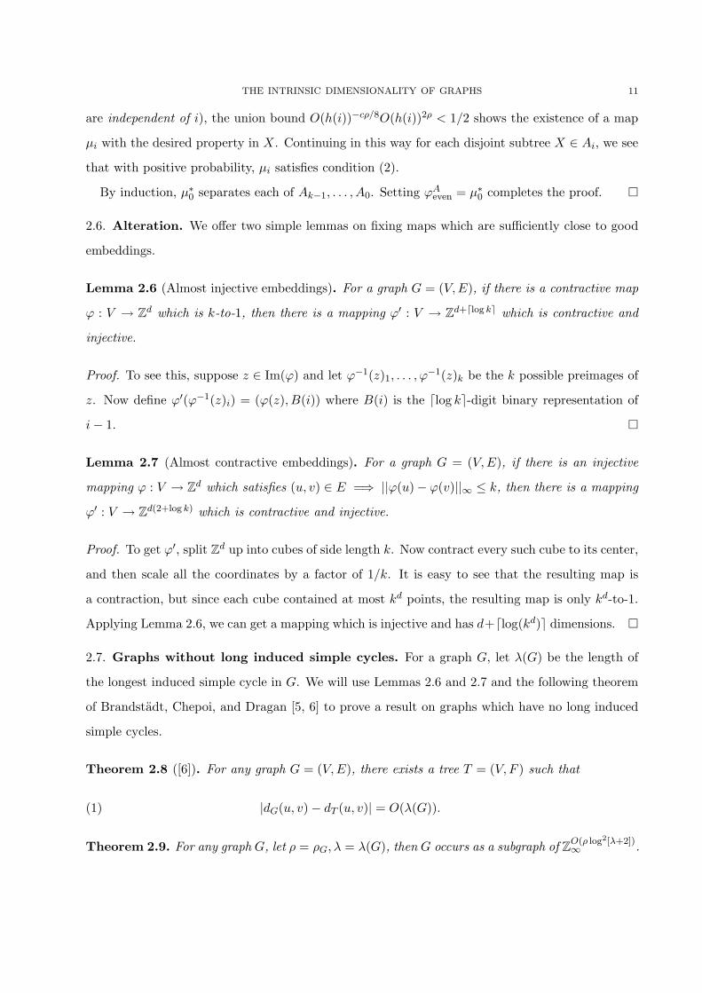
are independent of i), the union bound O(h(i))−cρ/8O(h(i))2ρ < 1/2 shows the existence of a map
µi with the desired property in X. Continuing in this way for each disjoint subtree X ∈ Ai, we see
that with positive probability, µi satisfies condition (2).
By induction, µ∗0 separates each of Ak−1, . . . , A0. Setting ϕAeven = µ∗0 completes the proof. ¤
2.6. Alteration. We offer two simple lemmas on fixing maps which are sufficiently close to good
embeddings.
Lemma 2.6 (Almost injective embeddings). For a graph G = (V, E), if there is a contractive map
ϕ : V → Zd which is k-to-1, then there is a mapping ϕ′ : V → Zd+dlog ke which is contractive and
injective.
Proof. To see this, suppose z ∈ Im(ϕ) and let ϕ−1(z)1, . . . , ϕ−1(z)k be the k possible preimages of
z. Now define ϕ′(ϕ−1(z)i) = (ϕ(z), B(i)) where B(i) is the dlog ke-digit binary representation of
i− 1. ¤
Lemma 2.7 (Almost contractive embeddings). For a graph G = (V, E), if there is an injective
mapping ϕ : V → Zd which satisfies (u, v) ∈ E =⇒ ||ϕ(u)− ϕ(v)||∞ ≤ k, then there is a mapping
ϕ′ : V → Zd(2+log k) which is contractive and injective.
Proof. To get ϕ′, split Zd up into cubes of side length k. Now contract every such cube to its center,
and then scale all the coordinates by a factor of 1/k. It is easy to see that the resulting map is
a contraction, but since each cube contained at most kd points, the resulting map is only kd-to-1.
Applying Lemma 2.6, we can get a mapping which is injective and has d+dlog(kd)e dimensions. ¤
2.7. Graphs without long induced simple cycles. For a graph G, let λ(G) be the length of
the longest induced simple cycle in G. We will use Lemmas 2.6 and 2.7 and the following theorem
of Brandstadt, Chepoi, and Dragan [5, 6] to prove a result on graphs which have no long induced
simple cycles.
Theorem 2.8 ([6]). For any graph G = (V,E), there exists a tree T = (V, F ) such that
|dG(u, v)− dT (u, v)| = O(λ(G)).(1)
Theorem 2.9. For any graph G, let ρ = ρG, λ = λ(G), then G occurs as a subgraph of ZO(ρ log2[λ+2])∞ .
12 ROBERT KRAUTHGAMER AND JAMES R. LEE
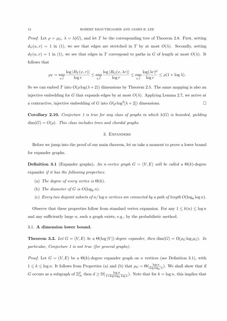
Proof. Let ρ = ρG, λ = λ(G), and let T be the corresponding tree of Theorem 2.8. First, setting
dG(u, v) = 1 in (1), we see that edges are stretched in T by at most O(λ). Secondly, setting
dT (u, v) = 1 in (1), we see that edges in T correspond to paths in G of length at most O(λ). It
follows that
ρT = supx,r
log |BT (x, r)|log r
≤ supx,r
log |BG(x, λr)|log r
≤ supx,r
log(λr)ρ
log r≤ ρ(1 + log λ).
So we can embed T into O(ρ log(λ + 2)) dimensions by Theorem 2.5. The same mapping is also an
injective embedding for G that expands edges by at most O(λ). Applying Lemma 2.7, we arrive at
a contractive, injective embedding of G into O(ρ log2[λ + 2]) dimensions. ¤
Corollary 2.10. Conjecture 1 is true for any class of graphs in which λ(G) is bounded, yielding
dim(G) = O(ρ). This class includes trees and chordal graphs.
3. Expanders
Before we jump into the proof of our main theorem, let us take a moment to prove a lower bound
for expander graphs.
Definition 3.1 (Expander graphs). An n-vertex graph G = (V, E) will be called a Θ(k)-degree
expander if it has the following properties:
(a) The degree of every vertex is Θ(k).
(b) The diameter of G is O(logk n).
(c) Every two disjoint subsets of n/ log n vertices are connected by a path of length O(logk log n).
Observe that these properties follow from standard vertex expansion. For any 1 ≤ k(n) ≤ log n
and any sufficiently large n, such a graph exists, e.g., by the probabilistic method.
3.1. A dimension lower bound.
Theorem 3.2. Let G = (V,E) be a Θ(log |V |)-degree expander, then dim(G) = Ω(ρG log ρG). In
particular, Conjecture 1 is not true (for general graphs).
Proof. Let G = (V,E) be a Θ(k)-degree expander graph on n vertices (see Definition 3.1), with
1 ≤ k ≤ log n. It follows from Properties (a) and (b) that ρG = Θ( log nlog logk n). We shall show that if
G occurs as a subgraph of Zd∞ then d ≥ Ω( log n1+log logk log n). Note that for k = log n, this implies that
THE INTRINSIC DIMENSIONALITY OF GRAPHS 13
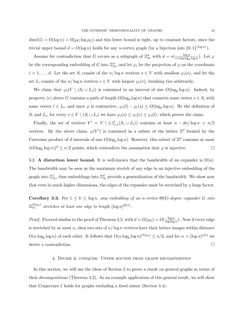
dim(G) = Ω(log n) = Ω(ρG log ρG) and this lower bound is tight, up to constant factors, since the
trivial upper bound d = O(log n) holds for any n-vertex graph (by a bijection into 0, 1dlog ne).
Assume for contradiction that G occurs as a subgraph of Zd∞ with d = o( log n1+log logk log n). Let ϕ
be the corresponding embedding of G into Zd∞, and let ϕi be the projection of ϕ on the coordinate
i = 1, . . . , d. Let the set Si consist of the n/ log n vertices v ∈ V with smallest ϕi(v), and let the
set Li consist of the n/ log n vertices v ∈ V with largest ϕi(v), breaking ties arbitrarily.
We claim that ϕi(V \ (Si ∪ Li)) is contained in an interval of size O(logk log n). Indeed, by
property (c) above G contains a path of length O(logk log n) that connects some vertex s ∈ Si with
some vertex l ∈ Li, and since ϕ is contractive, ϕi(l) − ϕi(s) ≤ O(logk log n). By the definition of
Si and Li, for every v ∈ V \ (Si ∪ Li) we have ϕi(s) ≤ ϕi(v) ≤ ϕi(l), which proves the claim.
Finally, the set of vertices V ′ = V \ (∪di=1(Si ∪ Li)) contains at least n − dn/ log n > n/2
vertices. By the above claim, ϕ(V ′) is contained in a subset of the lattice Zd formed by the
Cartesian product of d intervals of size O(logk log n). However, this subset of Zd contains at most
(O(logk log n))d ≤ n/2 points, which contradicts the assumption that ϕ is injective. ¤
3.2. A distortion lower bound. It is well-known that the bandwidth of an expander is Ω(n).
The bandwidth may be seen as the maximum stretch of any edge in an injective embedding of the
graph into Z1∞, thus embeddings into Zd∞ provide a generalization of the bandwidth. We show now
that even in much higher dimensions, the edges of the expander must be stretched by a large factor.
Corollary 3.3. For 1 ≤ k ≤ log n, any embedding of an n-vertex Θ(k)-degree expander G into
ZO(ρG)∞ stretches at least one edge to length (log n)Ω(1).
Proof. Proceed similar to the proof of Theorem 3.2, with d = O(ρG) = O( log nlog log n). Now if every edge
is stretched by at most α, then two sets of n/ log n vertices have their lattice images within distance
O(α logk log n) of each other. It follows that O(α logk log n)O(ρG) ≤ n/2, and for α = (log n)o(1) we
derive a contradiction. ¤
4. Divide & conquer: Upper bounds from graph decomposition
In this section, we will use the ideas of Section 2 to prove a result on general graphs in terms of
their decompositions (Theorem 4.2). As an example application of this general result, we will show
that Conjecture 1 holds for graphs excluding a fixed minor (Section 4.4).
14 ROBERT KRAUTHGAMER AND JAMES R. LEE
Outline. At a conceptual level, our embedding method for a general graph G bears some similarity
to the case of trees, although several technical aspects differ significantly. We cannot, for example,
form a coordinate by assigning edge weights independently at random (the weights along every
cycle would have to sum to 0). Here is an outline of the proof, with simplified notation and
constants. Our first step is to focus on a single “scale” r, and show a contraction ϕr such that
ϕr(u) 6= ϕr(v) for every two vertices u, v with r1/2 ≤ d(u, v) ≤ r. The construction of ϕr follows a
divide and conquer approach—we decompose the graph into (overlapping) “clusters”, embed each
cluster separately, and then “glue” these embeddings together. The decomposition guarantees that
for every pair u, v as above there exists at least one cluster C that contains them both, hence it
suffices that the embedding ϕC of this cluster satisfies ϕC(u) 6= ϕC(v). The decomposition further
guarantees that each cluster C has diameter at most rO(1), and then the growth rate bound implies
|C| ≤ rO(ρG).
One key difference between trees and general graphs is in the “divide” stage. For trees, we
were able to design such a decomposition directly (Section 2.3), using only two “layers”, i.e. two
partitions of V . When embedding general graphs, we consider decompositions with more layers,
but we must ensure that the number of layers is bounded by, say, O(1) or O(ρG), since it affects
the dimension of the resulting embedding. Furthermore, for trees our decompositions were nested
(in the sense that finer partitions were refinements of coarser ones); for general decompositions we
will have to force this nesting property to hold.
Another key difference is in the “conquer” (or combining) stage. In trees, it is quite easy to glue
embeddings of disjoint subtrees, using the concept of relative embeddings (Section 2.2). In general
graphs, we ensure that embeddings of disjoint clusters can be glued together by restricting ourselves
to cluster embeddings in which the “boundary” of the cluster is mapped to the all-zeros vector. One
side effect of this restriction is that for u, v ∈ C lying on or “close” to the boundary of C, we cannot
require that ϕC(u) 6= ϕC(v). In addition, to embed a single cluster C, we have to resort to a more
sophisticated method, inspired by Rao [21]; roughly speaking, we employ another decomposition
that breaks C into subclusters and map each subcluster independently at random. This inner
decomposition of C into subclusters has the same requirements as the outer decomposition, but it
is applied with a different parameter, namely—each subcluster’s diameter is less than r1/2. To show
that this embedding of C succeeds with high probability we use a union bound over the at most
THE INTRINSIC DIMENSIONALITY OF GRAPHS 15
|C|2 ≤ rO(ρG) pairs u, v ∈ C. Notice that the inner decomposition guarantees, for pairs u, v ∈ C as
above, that ϕC(u) and ϕC(v) are independent, while the outer decomposition limits the size of the
subproblem C, enabling the use of a union bound. On top of this, we have to adapt the technique
of conserving randomness (Section 2.5) to this new embedding method.
Preliminaries. In what follows, let G = (V,E) be a simple graph with growth rate ρ = ρG. A
cluster of G is a simply subset S ⊆ V , though we will usually use this terminology in the context
of a partition which contains S.
Define the boundary of a cluster S as ∂S = u ∈ S : ∃(u, v) ∈ E, v /∈ S. The boundary of a
collection C of clusters is defined as ∂C = ∪S∈C∂S. For a cluster S ⊆ V and a partition P of V ,
the induced partition (on the cluster S) is defined as Q = C ∩ S : C ∈ P \ ∅. As before, let
0 = (0, 0, . . . , 0) be the all-zero vector.
For u, v ∈ V let d(u, v) be the distance between u and v in the shortest path metric of G. We
stress that even when a particular cluster S is considered, d(u, v) denotes the distance in G and
not in S. In particular, define the diameter (sometimes called weak diameter) of S ⊆ V to be
diam(S) = supu,v∈S d(u, v). As usual, for S ⊆ V we define d(u, S) = infv∈S d(u, v).
The padded decomposition. We first discuss our method of choosing clusters. For the rest of
this section, fix an arbitrary constant α > 1. We will not explicitly state the dependence of other
constants on α, but it will be clear that any α = O(1) suffices for our purposes.
Definition 4.1 (The padded decomposition). A set P1, P2, . . . , Pm of m partitions of V is called
an r-padded decomposition of G with m layers if the following properties are satisfied.
(1) If C ∈ ∪mi=1Pi, then diam(C) ≤ rα.
(2) For every u ∈ V there exists some C ∈ ∪mi=1Pi such that B(u, 3r) ⊆ C.
We can now state our main result about embeddings obtained from graph decompositions. Its
proof appears in Section 4.3.
Theorem 4.2 (Embedding via decomposition). Let G be a graph with ρ = ρG. If for every 4 ≤r ≤ diam(G) there exists an r-padded decomposition of G with m layers, then dim(G) = O(m2ρ).
4.1. Relative embeddings. Suppose we are given a cluster S ⊆ V . Define a d-dimensional
relative embedding of S to be a contraction ϕ : S → Zd such that ϕ(∂S) = 0, i.e. the boundary
16 ROBERT KRAUTHGAMER AND JAMES R. LEE
is mapped to 0. Suppose further that we would like to find a relative embedding of S with the
following property (parameterized by r > 0): For every u, v ∈ S with d(u, v) > r and such that
B(u, 3r1/2) ⊆ S, we have ϕ(u) 6= ϕ(v). In other words, since we are imposing the rather stringent
condition that ϕ(∂S) = 0, we only make requirements on vertices that are far enough from the
boundary.
We will produce such an embedding using a technique inspired by the methods of Rao [21]. Each
coordinate is formed by partitioning S into clusters of diameter at most r, so u, v as above must
end up in different clusters. We then define the image of a vertex to be the distance from that
vertex to the boundary of its cluster. To achieve injectiveness with high probability, we “perturb”
the images by randomly contracting each cluster’s boundary inward.
For ease of notation, we define an r-inner decomposition to be an r1/α-padded decomposition; in
this case, clusters have diam(C) ≤ r and vertices have “padding” of the form B(u, 3r1/α). We now
show how to use an r-inner decomposition to produce a good relative embedding.
Lemma 4.3 (Relative embeddings). Suppose that G has an r-inner decomposition with m layers,
and let S ⊆ V be a cluster with |S| ≤ rO(ρ). Then there exists a relative embedding ϕ : S → ZO(mρ)
such that for every u, v ∈ S with d(u, v) > r and B(u, 3r1/α) ⊆ S, we have ϕ(u) 6= ϕ(v).
Proof. The m partitions produced by the r-inner decomposition induce m partitions Q1, . . . , Qm of
S (recall the definition of an induced partition). For each Qj we will construct a map ϕj : S → Zcαρ,
where c > 0 is a constant to be determined later.
Fix some partition Qj and form a single coordinate ϕ0j : S → Z as follows: For every C ∈ Qj ,
choose some rC ∈ 0, 1, . . . , r1/α uniformly at random and let ∂∗C = v ∈ C : d(v, ∂C) ≤ rC(this is the boundary of C randomly contracted inward). Now for each u ∈ S let Cu ∈ Qj be the
cluster containing u and define ϕ0j (u) = d(u, ∂∗Cu
). Recall that d(·, ·) denotes distance in G, and
thus ϕ0j (u) = max0, d(u, ∂Cu)− rCu.
Clearly ϕ0j (u) is a contraction, since (u, v) ∈ E implies that either u and v are in the same cluster
C ∈ Qj and then |d(u, ∂∗C)− d(v, ∂∗C)| ≤ 1, or each of them belongs to the boundary of its cluster
and then ϕ0j (u) = ϕ0
j (v) = 0. It is also clear that u ∈ ∂S implies u ∈ ∂C for some C ∈ Qj and
hence ϕ0j (u) = 0. Thus ϕ0
j (∂S) = 0.
THE INTRINSIC DIMENSIONALITY OF GRAPHS 17
Now independently form cαρ such coordinates (each time picking fresh values for the rC) and
let ϕj be the direct sum of the resulting maps, where c > 0 is a sufficiently large constant to be
determined later. Finally, set ϕ = ϕ1 ⊕ · · · ⊕ ϕm. From the properties of ϕj , we conclude that
ϕ : S → Zcmρ is a contraction which maps ∂S to 0, i.e., a relative embedding.
Consider a pair u, v with d(u, v) > r and such that B(u, 3r1/α) ⊆ S. It follows from property (2)
of Definition 4.1 that there exists a partition Qj of S and a subset C ∈ Qj for which B(u, 3r1/α) ⊆ C.
Since d(u, v) > r, the two vertices u and v must lie in different subsets of Qj . It follows that, in any
single coordinate ϕ0j of the map ϕj , the value of ϕ0
j (u) is distributed uniformly over an interval of
size r1/α independently of the value ϕ0j (v), hence Pr[ϕ0
j (u) = ϕ0j (v)] ≤ r−1/α. Thus the probability
that u and v collide in all cαρ coordinates of ϕj is Pr[ϕj(u) = ϕj(v)] ≤ r−cρ. Since |S| ≤ rO(ρ), there
are at most rO(2ρ) such pairs u, v, and hence the probability that there exists a pair that collides
is at most rO(2ρ)r−cρ < 1/2, if the constant c is chosen to be sufficiently large. The existence of a
map ϕ satisfying the lemma follows. ¤
4.2. A first attempt. Here is a simple approach which will fail in the end, but will give some
intuition as to how the padded decomposition will be used. We will use the padded decomposition
(Definition 4.1) to decompose G into layers of disjoint clusters. Using Section 4.1 we can then find
a relative embedding for each cluster; glueing all these embedding together, we shall arrive at a
good embedding for G. Note that the padded decomposition is being first to decompose the graph
G into clusters which will be separately embedded, and then inside each cluster to compute a good
relative embedding for that cluster.
Let k = dlog log diam(G)e, and set ri = 22ifor i ∈ 1, . . . , k, and r0 = 0. We apply an r-padded
decomposition with r = r1, . . . , rk. For each value of r, this decomposition will break the graph
into clusters of diameter at most rα such that every two vertices within a distance r are contained
in some such cluster S and are “far” from the boundary of S (as otherwise we cannot ensure that
they are “separated” by the relative embedding for S).
An embedding for one level. Assume that i > 1. Let P1, P2, . . . , Pm be the partitions
produced by the ri-padded decomposition. We will show how to construct a contraction ϕi : V →ZO(m2ρ) that satisfies: For every pair u, v ∈ V with ri−1 < d(u, v) ≤ ri, we have ϕi(u) 6= ϕi(v).
18 ROBERT KRAUTHGAMER AND JAMES R. LEE
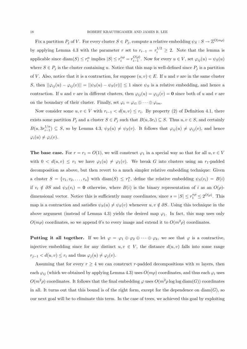
Fix a partition Pj of V . For every cluster S ∈ Pj , compute a relative embedding ψS : S → ZO(mρ)
by applying Lemma 4.3 with the parameter r set to ri−1 = r1/2i ≥ 2. Note that the lemma is
applicable since diam(S) ≤ rαi implies |S| ≤ rαρ
i = rO(ρ)i−1 . Now for every u ∈ V , set ϕij(u) = ψS(u)
where S ∈ Pj is the cluster containing u. Notice that this map is well-defined since Pj is a partition
of V . Also, notice that it is a contraction, for suppose (u, v) ∈ E. If u and v are in the same cluster
S, then ||ϕij(u) − ϕij(v)|| = ||ψS(u) − ψS(v)|| ≤ 1 since ψS is a relative embedding, and hence a
contraction. If u and v are in different clusters, then ϕij(u) = ϕij(v) = 0 since both of u and v are
on the boundary of their cluster. Finally, set ϕi = ϕi1 ⊕ · · · ⊕ ϕim.
Now consider some u, v ∈ V with ri−1 < d(u, v) ≤ ri. By property (2) of Definition 4.1, there
exists some partition Pj and a cluster S ∈ Pj such that B(u, 3ri) ⊆ S. Thus u, v ∈ S, and certainly
B(u, 3r1/αi−1) ⊆ S, so by Lemma 4.3, ψS(u) 6= ψS(v). It follows that ϕij(u) 6= ϕij(v), and hence
ϕi(u) 6= ϕi(v).
The base case. For r = r1 = O(1), we will construct ϕ1 in a special way so that for all u, v ∈ V
with 0 < d(u, v) ≤ r1 we have ϕ1(u) 6= ϕ1(v). We break G into clusters using an r1-padded
decomposition as above, but then revert to a much simpler relative embedding technique: Given
a cluster S = v1, v2, . . . , vs with diam(S) ≤ rα1 , define the relative embedding ψS(vi) = B(i)
if vi /∈ ∂S and ψS(vi) = 0 otherwise, where B(i) is the binary representation of i as an O(ρ)-
dimensional vector. Notice this is sufficiently many coordinates, since s = |S| ≤ rαρ1 ≤ 2O(ρ). This
map is a contraction and satisfies ψS(u) 6= ψS(v) whenever u, v /∈ ∂S. Using this technique in the
above argument (instead of Lemma 4.3) yields the desired map ϕ1. In fact, this map uses only
O(mρ) coordinates, so we append 0’s to every image and extend it to O(m2ρ) coordinates.
Putting it all together. If we let ϕ = ϕ1 ⊕ ϕ2 ⊕ · · · ⊕ ϕk, we see that ϕ is a contractive,
injective embedding since for any distinct u, v ∈ V , the distance d(u, v) falls into some range
rj−1 < d(u, v) ≤ ri and thus ϕj(u) 6= ϕj(v).
Assuming that for every r ≥ 4 we can construct r-padded decompositions with m layers, then
each ϕij (which we obtained by applying Lemma 4.3) uses O(mρ) coordinates, and thus each ϕi uses
O(m2ρ) coordinates. It follows that the final embedding ϕ uses O(m2ρ log log diam(G)) coordinates
in all. It turns out that this bound is of the right form, except for the dependence on diam(G), so
our next goal will be to eliminate this term. In the case of trees, we achieved this goal by exploiting
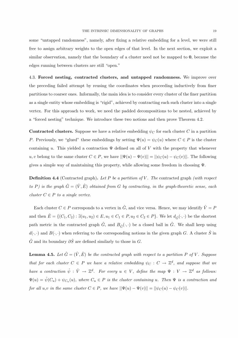
THE INTRINSIC DIMENSIONALITY OF GRAPHS 19
some “untapped randomness”, namely, after fixing a relative embedding for a level, we were still
free to assign arbitrary weights to the open edges of that level. In the next section, we exploit a
similar observation, namely that the boundary of a cluster need not be mapped to 0, because the
edges running between clusters are still “open.”
4.3. Forced nesting, contracted clusters, and untapped randomness. We improve over
the preceding failed attempt by reusing the coordinates when proceeding inductively from finer
partitions to coarser ones. Informally, the main idea is to consider every cluster of the finer partition
as a single entity whose embedding is “rigid”, achieved by contracting each such cluster into a single
vertex. For this approach to work, we need the padded decompositions to be nested, achieved by
a “forced nesting” technique. We introduce these two notions and then prove Theorem 4.2.
Contracted clusters. Suppose we have a relative embedding ψC for each cluster C in a partition
P . Previously, we “glued” these embeddings by setting Ψ(u) = ψC(u) where C ∈ P is the cluster
containing u. This yielded a contraction Ψ defined on all of V with the property that whenever
u, v belong to the same cluster C ∈ P , we have ||Ψ(u)−Ψ(v)|| = ||ψC(u)− ψC(v)||. The following
gives a simple way of maintaining this property, while allowing some freedom in choosing Ψ.
Definition 4.4 (Contracted graph). Let P be a partition of V . The contracted graph (with respect
to P ) is the graph G = (V , E) obtained from G by contracting, in the graph-theoretic sense, each
cluster C ∈ P to a single vertex.
Each cluster C ∈ P corresponds to a vertex in G, and vice versa. Hence, we may identify V = P
and then E = (C1, C2) : ∃(u1, u2) ∈ E, u1 ∈ C1 ∈ P, u2 ∈ C2 ∈ P. We let dG(·, ·) be the shortest
path metric in the contracted graph G, and BG(·, ·) be a closed ball in G. We shall keep using
d(·, ·) and B(·, ·) when referring to the corresponding notions in the given graph G. A cluster S in
G and its boundary ∂S are defined similarly to those in G.
Lemma 4.5. Let G = (V , E) be the contracted graph with respect to a partition P of V . Suppose
that for each cluster C ∈ P we have a relative embedding ψC : C → Zd, and suppose that we
have a contraction ψ : V → Zd. For every u ∈ V , define the map Ψ : V → Zd as follows:
Ψ(u) = ψ(Cu) + ψCu(u), where Cu ∈ P is the cluster containing u. Then Ψ is a contraction and
for all u,v in the same cluster C ∈ P , we have ||Ψ(u)−Ψ(v)|| = ||ψC(u)− ψC(v)||.
20 ROBERT KRAUTHGAMER AND JAMES R. LEE
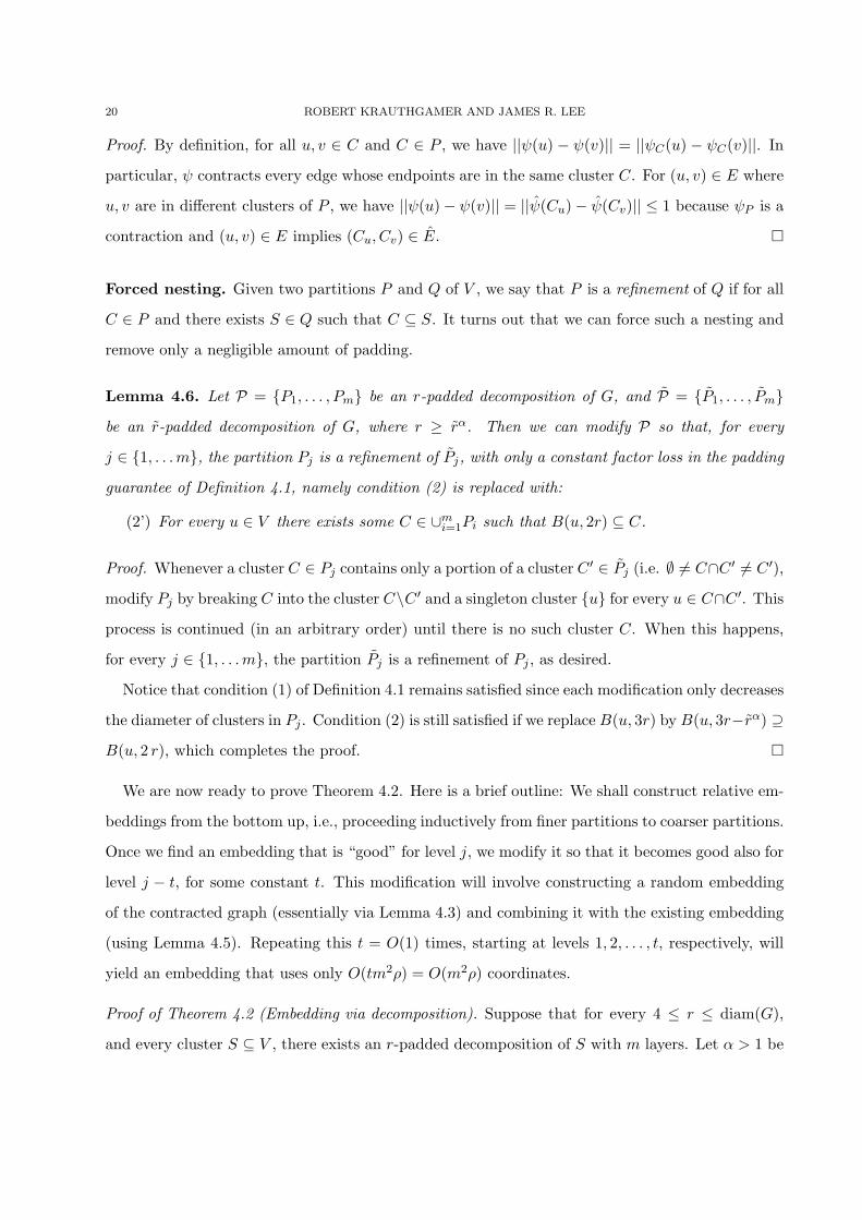
Proof. By definition, for all u, v ∈ C and C ∈ P , we have ||ψ(u) − ψ(v)|| = ||ψC(u) − ψC(v)||. In
particular, ψ contracts every edge whose endpoints are in the same cluster C. For (u, v) ∈ E where
u, v are in different clusters of P , we have ||ψ(u)− ψ(v)|| = ||ψ(Cu)− ψ(Cv)|| ≤ 1 because ψP is a
contraction and (u, v) ∈ E implies (Cu, Cv) ∈ E. ¤
Forced nesting. Given two partitions P and Q of V , we say that P is a refinement of Q if for all
C ∈ P and there exists S ∈ Q such that C ⊆ S. It turns out that we can force such a nesting and
remove only a negligible amount of padding.
Lemma 4.6. Let P = P1, . . . , Pm be an r-padded decomposition of G, and P = P1, . . . , Pmbe an r-padded decomposition of G, where r ≥ rα. Then we can modify P so that, for every
j ∈ 1, . . .m, the partition Pj is a refinement of Pj, with only a constant factor loss in the padding
guarantee of Definition 4.1, namely condition (2) is replaced with:
(2’) For every u ∈ V there exists some C ∈ ∪mi=1Pi such that B(u, 2r) ⊆ C.
Proof. Whenever a cluster C ∈ Pj contains only a portion of a cluster C ′ ∈ Pj (i.e. ∅ 6= C∩C ′ 6= C ′),
modify Pj by breaking C into the cluster C\C ′ and a singleton cluster u for every u ∈ C∩C ′. This
process is continued (in an arbitrary order) until there is no such cluster C. When this happens,
for every j ∈ 1, . . . m, the partition Pj is a refinement of Pj , as desired.
Notice that condition (1) of Definition 4.1 remains satisfied since each modification only decreases
the diameter of clusters in Pj . Condition (2) is still satisfied if we replace B(u, 3r) by B(u, 3r−rα) ⊇B(u, 2 r), which completes the proof. ¤
We are now ready to prove Theorem 4.2. Here is a brief outline: We shall construct relative em-
beddings from the bottom up, i.e., proceeding inductively from finer partitions to coarser partitions.
Once we find an embedding that is “good” for level j, we modify it so that it becomes good also for
level j − t, for some constant t. This modification will involve constructing a random embedding
of the contracted graph (essentially via Lemma 4.3) and combining it with the existing embedding
(using Lemma 4.5). Repeating this t = O(1) times, starting at levels 1, 2, . . . , t, respectively, will
yield an embedding that uses only O(tm2ρ) = O(m2ρ) coordinates.
Proof of Theorem 4.2 (Embedding via decomposition). Suppose that for every 4 ≤ r ≤ diam(G),
and every cluster S ⊆ V , there exists an r-padded decomposition of S with m layers. Let α > 1 be
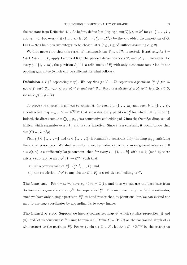
THE INTRINSIC DIMENSIONALITY OF GRAPHS 21
the constant from Definition 4.1. As before, define k = dlog log diam(G)e, ri = 22ifor i ∈ 1, . . . , k,
and r0 = 0. For every i ∈ 1, . . . , k let Pi = P i1, . . . , P
im be the ri-padded decomposition of G.
Let t = t(α) be a positive integer to be chosen later (e.g., t ≥ α3 suffices assuming α ≥ 2).
We first make sure that this series of decompositions P1, . . . ,Pk is nested. Iteratively, for i =
t + 1, t + 2, . . . , k, apply Lemma 4.6 to the padded decompositions Pi and Pi−t. Thereafter, for
every j ∈ 1, . . . m, the partition P i−tj is a refinement of P i
j with only a constant factor loss in the
padding guarantee (which will be sufficient for what follows).
Definition 4.7 (A separating map). We say that ϕ : V → Zd separates a partition P ij if, for all
u, v ∈ V such that ri−1 < d(u, v) ≤ ri and such that there is a cluster S ∈ P ij with B(u, 2ri) ⊆ S,
we have ϕ(u) 6= ϕ(v).
To prove the theorem it suffices to construct, for each j ∈ 1, . . . ,m and each i0 ∈ 1, . . . , t,a contractive map ϕi0,j : V → ZO(mρ) that separates every partition P i
j for which i ≡ i0 (mod t).
Indeed, the direct sum ϕ =⊕
i0,j ϕi0,j is a contractive embedding of G into the O(tm2ρ)-dimensional
lattice, which separates every P ji and is thus injective. Since t is a constant, it would follow that
dim(G) = O(m2ρ).
Fixing j ∈ 1, . . . , m and i0 ∈ 1, . . . , t, it remains to construct only the map ϕi0,j satisfying
the stated properties. We shall actually prove, by induction on i, a more general assertion: If
c = c(t, α) is a sufficiently large constant, then for every i ∈ 1, . . . , k with i ≡ i0 (mod t), there
exists a contractive map ψi : V → Zcmρ such that
(i) ψi separates each of P i0j , P i0+t
j , . . . , P ij , and
(ii) the restriction of ψi to any cluster C ∈ P ij is a relative embedding of C.
The base case. For i = i0 we have ri0 ≤ rt = O(1), and thus we can use the base case from
Section 4.2 to generate a map ψi0 that separates P i0j . This map need only use O(ρ) coordinates,
since we have only a single partition P i0j at hand rather than m partitions, but we can extend the
map to use cmρ coordinates by appending 0’s to every image.
The inductive step. Suppose we have a contractive map ψi which satisfies properties (i) and
(ii), and let us construct ψi+t using Lemma 4.5. Define G = (V , E) as the contracted graph of G
with respect to the partition P ij . For every cluster C ∈ P i
j , let ψC : C → Zcmρ be the restriction
22 ROBERT KRAUTHGAMER AND JAMES R. LEE
of ψi to C; by the induction hypothesis, ψC is a relative embedding of C. It remains to define an
embedding ψ : V → Zcmρ, and then we can let ψi+t : V → Zcmρ be the map yielded by Lemma 4.5.
Since V = P ij is a refinement of P i+t
j , the latter naturally yields a partition P i+tj of V , as follows.
With every cluster S ∈ P i+tj we associate a cluster S = C ∈ V : C ⊆ S in G. It is then easy to
verify that P i+tj = S : S ∈ P i+t
j is a partition of V .
Below, we shall define the mapping ψ on a single cluster S ∈ P i+tj in G. By construction, ψ
will be a relative embedding of that cluster S (with respect to G) i.e. ψ(∂S) = 0, and thus the
resulting embedding will necessarily be a contractive embedding of the entire V . In fact, we shall
define ψ on each S randomly.
Fix a cluster S ∈ P i+tj and the corresponding S ∈ P i+t
j . Now construct an “inner decomposition”
for S, as follows: Take an m-layer r1/αi+t -inner decomposition of G (note that r
1/α2
i+t ≥ 4), and force P ij
to be a refinement of each layer of this inner decomposition using Lemma 4.6. The forced nesting
procedure is applicable because r1/α2
i+t ≥ rαi . This procedure modifies only the inner decomposition
(and not P ij ), changing its padding guarantee to 2r1/α2
i+t . Each layer of the inner decomposition is a
partition of V , and hence induces a partition of S. Denote these m partitions of S by Q1, . . . , Qm.
Since P ij is a refinement of the inner decomposition, each partition Ql of S naturally yields a
partition of S which we shall denote by Ql. (This is similar to the way P i+tj was defined.)
We generate the map ψ : S → Zcαmρ in a random fashion, using an argument similar to Lemma
4.3.1 Fix a partition Ql and form a single coordinate f : S → Z randomly as follows: For every
C ∈ Ql choose a value rC ∈ 0, 1, . . . , ri uniformly at random and let f(w) = max0, dG(w, ∂Ql).Now independently form cαρ such coordinates (each time picking fresh values for the rC), and let
ψl : S → Zcαρ be the direct sum of the resulting maps. We apply the above to every partition Ql
and set ψ = ψ1 ⊕ · · · ⊕ ψm.
Notice that once ψ is defined on S, the map ψi+t yielded by Lemma 4.5 is defined on S. Since
the former map is constructed in a random fashion, the latter mapping is randomized as well. The
next two lemmas analyze this randomized embedding of S.
Claim 4.8. Fix S ∈ P i+tj . Then ψi+t : S → Zcαmρ is a relative embedding of S.
1Applying this lemma directly to S would generate ψ such that ψ(C) 6= ψ(C′) for certain C, C′ ∈ V , but it does notguarantee that as a result ψi+t(u) 6= ψi+t(v) for suitable u ∈ C, v ∈ C′.
THE INTRINSIC DIMENSIONALITY OF GRAPHS 23
Proof. Let us first show that ψ : S → Zcαρ is a relative embedding of S (with respect to G). Indeed,
it is easy to see that every coordinate f generated as above using some partition Ql is a contraction,
and that for every vertex w ∈ ∂S, we have w ∈ ∂Ql and hence f(w) = 0. It follows that ψ, which
is a direct sum of such maps f , is a relative embedding of S.
Now consider ψi+t; we know it is a contraction from Lemma 4.5, so we only need to show that
ψi+t(∂S) = 0. Fix u ∈ ∂S and let Cu ∈ P ij be the cluster containing u. Then u ∈ ∂Cu (recall that
Cu ⊆ S) and thus ψCu(u) = 0. It also follows that Cu ∈ ∂S, and hence ψ(Cu) = 0. By definition,
ψi+t(u) = ψ(Cu) + ψCu(u) = 0, which proves the claim. ¤
Claim 4.9. Fix S ∈ P i+tj . Then with probability at least 1/2, for all u, v ∈ S with ri+t−1 <
d(u, v) ≤ ri+t and with B(u, 2ri+t) ⊆ S, we have ψi+t(u) 6= ψi+t(v).
Proof. Fix u, v ∈ S with ri+t−1 < d(u, v) ≤ ri+t and B(u, 2ri+t) ⊆ S. Let Cu ∈ P ij be the cluster
containing u, and let Cv ∈ P ij be similarly for v. Clearly, u, v ∈ S ∈ P i+t
j ; recalling that P ij is a
refinement of P i+tj we get that Cu, Cv ∈ S.
The ball B = B(u, 2r1/α2
i+t ) is contained in some cluster of the inner decomposition, even after
the forced nesting with P ij . By the above, B ⊆ S and thus B is entirely contained also in some
cluster of some partition Ql of S. Since clusters in P ij have diameter at most rα (in G), we have:
(a) ri+t−1/rαi < dG(Cu, Cv) ≤ ri+t.
(b) BG(Cu, 2r1/α2
i+t /rαi ) is entirely contained in some cluster of Ql.
Now consider ψl(Cu) and ψl(Cv). Clusters in Ql have diameter (in G) at most r1/αi+t ≤ ri+t−1/rα
i ,
so (a) implies that Cu and Cv reside in different clusters of Ql. This, in conjunction with (b)
(and because 2r1/α2
i+t /rαi ≥ ri), implies that each coordinate of ψl(Cu) is distributed uniformly over
an interval of size ri, independently of the corresponding coordinate in ψ(Cv). Recalling that
ψ = ψ1 ⊕ · · · ⊕ ψm, ψi+t(u) = ψi(u) + ψ(Cu), and ψi+t(v) = ψi(v) + ψ(Cv), we get that each of at
least cαρ coordinates of ψi+t(u) is distributed uniformly over an interval of size ri, independently
of the corresponding coordinate in ψi+t(v). Therefore,
Pr[ψi+t(u) = ψi+t(v)] ≤ r−cαρi .
The number of pairs u, v ∈ S is at most |S|2 ≤ (rαi+t)
2ρ = r2t+1αρi , the claim follows via a union
bound if only we choose the constant c ≥ 2t+2. ¤
24 ROBERT KRAUTHGAMER AND JAMES R. LEE
As mentioned before, we use the preceding claim to construct for every S ∈ P i+tj a map ψ : S →
ZO(mρ). This collection of maps gives an embedding ψ : V → ZO(mρ), and using Lemma 4.5 we
produce from it an embedding ψi+t : V → ZO(mρ) that satisfies the induction hypothesis for i + t,
and this completes the proof of Theorem 4.2. ¤
4.4. Graphs excluding a fixed minor. Let G be a graph that excludes a Ks,s minor for some
fixed s. By adapting a decomposition technique of Klein, Plotkin, and Rao [14] we construct, for
any value r ≥ 1, an r-padded decomposition of G with only O(2s) layers. Applying Theorem 4.2,
we then arrive at the main result of this section.
Theorem 4.10 (Excluded minor families). Conjecture 1 is true for any family of graphs that
excludes a fixed minor. For such graphs, dim(G) = O(ρG).
Proof. By Theorem 4.2 it suffices to show how to produce an r-padded decomposition with m = 2s
layers for any graph that excludes a Ks,s minor, as this implies that dim(G) ≤ O(4sρG).
To this end, consider such a graph G = (V,E) and fix a value r. First, construct a Breadth-
First-Search (BFS) tree from an arbitrary vertex v ∈ V , and compute for every vertex its BFS level
(i.e., its distance from v). Then cut the tree every 12r BFS levels by removing any edge connecting
a vertex of BFS-level j to a vertex of BFS-level j + 1 for any j ≡ 0 (mod 12r). Let C0 denote the
resulting set of connected components of G. Next, take another copy of G and cut it similarly but
starting from BFS level 6r, i.e., remove any edge connecting a vertex of BFS-level j to a vertex of
BFS-level j +1 for any j ≡ 6r (mod 12r). Let C1 denote the resulting set of connected components
of G. Now for each Ci, apply the same procedure on all the connected components in Ci, namely,
choose an arbitrary vertex, construct a BFS tree, and form two sets of connected components Ci0
and Ci1 by making the cuts as above (staggered, each at intervals of size 12r). Repeat this process
s times and let Cq for q ∈ 0, 1s denote the 2s final sets of connected components. From [14] we
know that every connected component in every final Cq has diameter at most O(r). In addition,
for every vertex u the entire ball B(u, 3r) is uncut in at least one final set Cq, because each step
performs two different sets of “staggered” cuts, at least one of which must avoid the entire ball
B(u, 3r). ¤
THE INTRINSIC DIMENSIONALITY OF GRAPHS 25
5. A general dimension upper bound
In this section we give a tight upper bound on the dimension of general graphs: dim(G) =
O(ρG log ρG) for any graph G. (In Section 3, we showed that this upper bound is met by expanders.)
First, we devise a decomposition for growth-restricted metrics (Section 5.1) and use Theorem 4.2 to
obtain a weaker upper bound of O(ρ3G) (Section 5.2). Then, by combining the previous arguments
more carefully and utilizing some Chernoff-type tail bounds, we obtain the aforementioned tight
upper bound (Section 5.3). We shall use some terminology from Section 5.2.
5.1. Partitioning of growth-restricted graphs. Linial and Saks [17] and Bartal [3] show that
for any graph G = (V,E) and 1 ≤ r ≤ diam(G), there exists a probabilistic partitioning of G into
disjoint clusters of diameter at most O(r ln |V |), such that for any pair of vertices u, v ∈ V , the
probability that u and v end up in different clusters is at most d(u, v)/r. Let ρ = ρG. In this
section, we give a similar decomposition, but we replace the diameter bound of O(r ln |V |) with a
bound that is independent of |V |, namely O(ρ r ln r), for any r ≥ ρ. Our partitioning method is
similar to those of [17] and [3], but different in a subtle and crucial way: It is local. Events which
are sufficiently far apart are mutually independent.
First, take the continuous exponential distribution with mean r > 0, truncate it at some value
M > 0 and rescale the remaining density function. The resulting distribution, which we denote
Texp(r,M), has density function p(z) = eM/r
r(eM/r−1)e−z/r for z ∈ (0,M).
The partitioning procedure. Let V = v1, v2, . . . , vn and let r ≥ ρ. For each vt ∈ V ,
choose independently a radius rt according to the distribution Texp(r, 8ρr ln r). Now define St =
B(vt, rt) \ ∪t−1i=1B(vi, ri) as the set of vertices v for which B(vt, rt) is the first ball containing v.
Finally, define the set of clusters to be C = S1, . . . , Sn.
It is easy to see that C is a partition of V , and that the (weak) diameter of every cluster C ∈ Cis bounded by diam(C) ≤ 16ρr ln r. Further analysis will require the following simple facts. In
particular, (3) shows that if M ≥ 2r, the truncated exponential distribution is “almost” memoryless.
Fact 5.1. Consider a random variable R ∼ Texp(r,M) for M ≥ 2r > 0. Then,
(1) For all β ≥ 0, Pr[R ≥ β] ≤ 2e−β/r.
(2) For all β ≥ 0, Pr[R ≤ β] ≤ 2(1− e−β/r) ≤ 2β/r.
26 ROBERT KRAUTHGAMER AND JAMES R. LEE
(3) For all β ≥ 0 and R0 ≤ M/2, Pr[R ≤ R0 + β |R ≥ R0] ≤ 2β/r.
For a vertex u ∈ V and x ≥ 0, let Exu be the event that B(u, x) is split between multiple clusters,
i.e., that no cluster C ∈ C fully contains B(u, x).
Lemma 5.2. Let u ∈ V and r ≥ 16ρ, and x ≥ 0. Then Pr[Exu ] ≤ 10x/r.
Proof. Assume x ≤ r (the theorem says nothing for larger x) and let B = B(u, x), Bt = B(vt, rt).
Let us say that the ball B is cut by the ball Bt if ∅ 6= St ∩ B 6= B while for all i < t, Si ∩ B = ∅. Exu
is precisely the event that there is a ball Bt that cuts B. Let us separate these balls Bt into two
classes, depending on the distance from vt to u. Define Efar to be the event that there exists Bt
that cuts B and d(vt, u) ≥ 4ρr ln r. Define Enear to be the event that there exists Bt that cuts Band d(vt, u) < 4ρr ln r.
Fix vt with d(vt, u) ≥ 4ρr ln r and notice that by Fact 5.1,
Pr[Bt cuts B] ≤ Pr[rt ≥ 4ρr ln r − x] ≤ 2r−4ρex/r ≤ 6r−4ρ.
But the number of such vt for which Bt can possibly cut B is at most the number of vertices in a
ball of radius 8ρr ln r + x ≤ r3 which is at most r3ρ. Taking a union bound over all such possible
vt, we see that Pr[Efar] ≤ 6r−4ρr3ρ ≤ 6/rρ ≤ 6/r. Thus we are left only to bound the probability of
Enear.
Let the random variable T be the minimum t such that BT ∩B 6= ∅ (note that possibly vT ∈ B).
The ball BT can either cut B (in which case Exu occurs) or contain B (and then B ⊆ ST is not cut
by any ball Bt). By the principle of deferred decision it suffices to upper bound the conditional
probability Pr[Enear|T = t] for an arbitrary t. To this end, we may assume that d(vt, u) ≤ 4ρr ln r
(as otherwise this conditional probability is 0) and then Enear happens if and only if Bt cuts B,
which in turn happens only if rt ≤ d(vt, u) + x. Hence,
Pr[Enear |T = t] ≤ Pr[rt ≤ d(vt, u) + x | rt ≥ d(vt, u)− x
] ≤ 4x
r,
where we have used Fact 5.1 in conjunction with d(vt, u) ≤ 4ρr ln r. Thus, Pr[Enear] =∑
t Pr[T =
t] · Pr[Enear|T = t] ≤ 4x/r and Pr[Exu ] ≤ Pr[Enear] + Pr[Efar] ≤ 10x/r. ¤
5.2. Layered decomposition of growth-restricted graphs. Now we describe how to obtain
an r-padded decomposition with O(ρG) layers for general graphs G. Plugging these values into
THE INTRINSIC DIMENSIONALITY OF GRAPHS 27
Theorem 4.2 yields an embedding into O(ρ3G) dimensions. We will only be able to show the existence
of such decompositions under the assumption that r ≥ ρ. In the case where r ≤ 16ρ, clusters of
diameter rO(1) have at most ρO(ρ) points, so we will be able to embed these by brute force using
only O(ρ log ρ) dimensions (similar to the base case of Section 4.2). The final result appears in
Theorem 5.5.
Theorem 5.3 (Decomposition theorem). For every graph G = (V,E) and every r ≥ 16ρG, there
exists an r-padded decomposition with m = O(ρG) layers.
Proof. Let ρ = ρG and assume r ≥ 16ρ. To produce a single layer of the decomposition (a
partition of V into clusters), we will use the procedure of Section 5.1, with the parameter r (in that
procedure and in Lemma 5.2) set to r2. Notice that the clusters produced have diameter at most
32ρr2 ln r ≤ r4. For a vertex v ∈ V , let Ev be the event that the ball of radius 3r about v is cut
(i.e., split amongst two or more clusters). From Lemma 5.2, we know that Pr[Ev] ≤ 3/r.
Now produce m layers independently (with fresh random coins each time) and let Emv be the
event that the ball of radius 3r about v is cut in every layer. Clearly Pr[Emv ] ≤ (3/r)m. We would
like to say that Pr[∧
v∈V Emv
]> 0. If we could show this with m = O(ρ), the theorem would follow.
And indeed, this is our goal. We will employ the following symmetric form of the Lovasz Local
Lemma, see e.g. [1].
Lemma 5.4 (Lovasz Local Lemma). Let A1, . . . , An be events in an arbitrary probability space.
Suppose that for each Ai there is a set that contains all but at most d of the other events Aj, such
that Ai is mutually independent of this set of events. If for all i ∈ 1, . . . , n we have Pr[Ai] ≤ p,
and ep(d + 1) ≤ 1, then Pr[∧ni=1Ai] > 0.
Let r1 = 2r3 ln r+6r. An event Emu is mutually independent of all events Em
v for which d(u, v) > r1
because every ball in the partitioning of Section 5.1 has radius at most r3 ln r and thus cannot
intersect both B(u, 3r) and B(v, 3r). It follows that Emu is mutually independent of the set of all
events Emv except those for which v ∈ B(u, r1), and there are at most d = rρ
1 such vertices v. Thus
if Pr[Emu ] ≤ 1/e(d + 1), we can apply the local lemma and the theorem is proved. But this is easily
accomplished by choosing say m = d8ρe. By applying Lemma 5.4 we conclude that there exists an
r-padded decomposition for V (with α = 4). ¤
28 ROBERT KRAUTHGAMER AND JAMES R. LEE
Theorem 5.5. For every graph G with growth rate ρG, dim(G) = O(ρ3G).
Proof (sketch). We provide only a sketch of the proof, since a better upper bound is given in
the next section. We use the proof of Theorem 4.2, except that instead of the induction’s base
case being r = O(1), we start with a level corresponding to r = ρO(1). In this case, clusters
have diameter rO(1) = ρO(1), so we can easily give a relative embedding for each cluster using
only O(ρ log ρ) coordinates, similar to the base case of 4.2. The rest of the proof then proceeds
unchanged, including the inductive step in which we use the decomposition provided by Theorem
5.3. ¤
Remark: Algorithmiziation of the Local Lemma. Although most of the techniques in this
paper can easily be interpreted algorithmically, this is not immediately obvious for our use of the
local lemma. Fortunately, it is not difficult to see that standard techniques suffice (see, e.g., [1,
Chapter 5]).
5.3. A tight upper bound. As mentioned previously, Theorem 5.3, combined with Theorem 4.2,
shows that dim(G) = O(ρ3G) for every graph G. By carefully combining the previous arguments
and utilizing some Chernoff-type tail bounds, we are able to find a tight upper bound, dim(G) =
O(ρG log ρG); see Theorem 5.8 below.
We first strengthen the decomposition of Theorem 5.3. Given m layers (partitions of V ) P1, P2, . . . , Pm,
we say that a vertex u ∈ V is padded in a layer j if there exists a cluster C ∈ Pj such that
B(u, 3r) ⊆ C (otherwise, we say that u is unpadded in layer j). We next show a decomposition in
which every vertex is padded in most of the layers (rather than in one layer).
Theorem 5.6 (Strengthened decomposition theorem). For every graph G = (V, E) and every
r ≥ 36ρG, there exists an r-padded decomposition with m = O(ρG) layers, in which:
(2”) For every u ∈ V there are 34m partitions Pj in which there is C ∈ Pj with B(u, 3r) ⊆ C.
Proof. Similar to the proof of Theorem 5.3, we construct m = O(ρG) layers of randomized partitions
that always satisfy requirement (1), and argue that, with positive probability, requirement (2”) is
satisfied. The probability that u is unpadded in a single layer is at most 3/r (this followed from
Lemma 5.2), so the expected number of layers in which u is unpadded is at most 3m/r. We now
need the following Chernoff-type tail bound (see, e.g., [20, Chapter 4]).
THE INTRINSIC DIMENSIONALITY OF GRAPHS 29
Lemma 5.7 (A tail bound). Let X1, X2, . . . , Xn be independent Poisson trials such that, for 1 ≤i ≤ n, Pr[Xi = 1] = pi and 0 < pi < 1. Then for X =
∑i Xi, µ = E[X], and any δ > 0,
Pr[X > (1 + δ)µ] <
(eδ
(1 + δ)1+δ
)µ
<
(e
1 + δ
)(1+δ)µ
.
Let mu be the expected number of layers in which a vertex u is unpadded, and let Eu be the
event that u is unpadded in more than 14m layers. Then, applying the above lemma,
Pr[Eu] = Pr[Yu >
r
12· 3m
r
]≤ 1
(r/12e)m/4.
Applying Lemma 5.4 the same way we did in the proof of Theorem 5.3 for a suitable m = O(ρG),
we conclude that Pr[∧
v∈V Emv
]> 0. ¤
Theorem 5.8 (Embedding of general graphs). For every graph G = (V,E) with growth rate ρG,
dim(G) = O(ρG log ρG).
Proof. We adapt the proof of Theorem 4.2, as follows. First, we use the strengthened decomposition
from Theorem 5.6. Second, we employ a more careful analysis that exploits the independence of
coordinates constructed from different layers together with the local lemma, instead of applying a
union bound separately in each cluster.
In the sequel, we describe the modifications to that proof. In fact, we will only show that any one
level (in the sense of Section 4.2) can be embedded into O(ρ log ρ) dimensions. Using the nesting
techniques of Section 4.3, the existence of a contractive and injective embedding that uses only
O(ρ log ρ) coordinates follows.
Let ρ = ρG. Fix r = 22iand suppose we are given an r-padded decomposition with m = O(ρ)
layers P1, P2, . . . , Pm strengthened as per Theorem 5.6. We may assume further that m ≥ ρ, because
otherwise we can just duplicate every layer dρ/me times. Let c > 0 be a constant to be determined
later. We shall construct, for each cluster S ∈ Pj , a relative embedding ψS : S → Zc log ρ, such that
for all u, v ∈ V with√
r < d(u, v) ≤ r there exist a layer Pj and a cluster S ∈ Pj such that u, v ∈ S
and ψS(u) 6= ψS(v). Letting ϕj(u) = ψSu(u) where Su ∈ Pj is the cluster containing u, and setting
ϕ = ⊕mj=1ϕj , we will conclude that ϕ(u) 6= ϕ(v) for all u, v ∈ V with
√r < d(u, v) ≤ r. As before,
in the base case we shall replace the requirement√
r < d(u, v) ≤ r with 0 < d(u, v) ≤ r.
30 ROBERT KRAUTHGAMER AND JAMES R. LEE
The base case. Assume 16ρ ≤ r ≤ ρO(1) (note that this is where our decomposition breaks down).
We produce, for every cluster S ∈ Pj , a relative embedding ψS : S → Zc log ρ as follows: If u /∈ ∂S,
then let ψS(u) be a (c log ρ)-dimensional vector chosen uniformly at random from 0, 1c log ρ, and
let ψS(u) = 0 otherwise. This ψS is clearly a contraction.
Consider two vertices u, v with 0 < d(u, v) ≤ r and let Pj be a layer in which u is padded. In this
layer, u and v belong to the same cluster S ∈ Pj and u /∈ ∂S, so Pr[ψS(u) = ψS(v)] ≤ (12)c log ρ = ρ−c.
Let Eu,v be the event that, in the resulting embedding ϕ = ⊕mj=1ϕj , we have ϕ(u) = ϕ(v). For this
event to happen, it must be that in every layer in which u is padded, we have ψS(u) = ψS(v). It
then follows that
Pr[Eu,v] = Pr[ϕ(u) = ϕ(v)] ≤ ρ−cm/2 ≤ ρ−cρ/2.
There are Ω(|V |) events Eu,v and we would like to argue that with positive probability, none of them
occur. Again, the local lemma comes to our rescue. It is not difficult to see that Eu,v is independent
of all events Eu′,v′ for which d(u, u′) > r (because the image of u is chosen independently of the
images of all the corresponding v, u′, and v′). It follows that Eu,v is mutually independent of all
but at most d = r2ρ ≤ ρO(ρ) other events. Choosing the constant c to be a large enough relative to
the constants in the bound r ≤ ρO(1), we see that Pr[Eu,v] ≤ ρ−cρ/2 ≤ 1/e(d + 1). Thus, applying
Lemma 5.4 yields an embedding for which none of the events Eu,v occur.
Higher levels. Assume r ≥ (16ρ)2. Recall that in Theorem 4.2, for each layer Pj and each cluster
S ∈ Pj , we produced a random relative embedding ψS : S → ZO(m log ρ) by constructing (using
Lemma 4.3) O(log ρ) coordinates from each layer of an m-layer r1/2-inner decomposition. Here,
instead, for each S ∈ Pj we shall produce a random relative embedding ψS : S → Zc (which is
of course stronger than using O(log ρ) coordinates), by constructing only c = O(1) coordinates
from layer j of the inner decomposition. More formally, take an m-layer r1/2-inner decomposition
of G. Now for each Pj and each cluster S ∈ Pj , construct each of the c coordinates of ψS as
follows (this is analogous to Lemma 4.3): Let Qj be the partition of S induced by layer j of
the inner decomposition. For every cluster C ∈ Qj , choose rC ∈ 0, 1, . . . , r1/2α uniformly at
random. For every u ∈ S, let Cu ∈ Qj be the cluster containing u, and define the image of u to be
max0, d(u, ∂Cu)− rCu. Clearly, ψS is a relative embedding of S.
THE INTRINSIC DIMENSIONALITY OF GRAPHS 31
Consider two vertices u, v with√
r < d(u, v) ≤ r. Since u is padded in at least 34m layers each
decomposition (i.e., the layers P1, . . . , Pm and in the inner decomposition), we see that for at
least 12m values of j, the vertex u is padded both in Pj and in layer j of the inner decomposition.
Fix such j, and let S ∈ Pj be the cluster containing u. It follows that u, v belong to the same
cluster S ∈ Pj , but to different clusters of the inner decomposition. Since u is padded in layer j
of the inner decomposition, each coordinate of ψS(u) is chosen at random from an interval of size
at least r−1/2α, independently of ψS(v), and thus the probability it collides with the corresponding
coordinate of ψS(v) is at most r−1/2α. Hence,
Pr[ϕj(u) = ϕj(v)] = Pr[ψS(u) = ψS(v)] ≤ r−c/2α,
and the embedding ϕ = ⊕mj=1ϕj satisfies Pr[ϕ(u) = ϕ(v)] ≤ r−cm/4α ≤ r−cρ/4α. Finally, we
would like to apply Lemma 5.4 on the events Eu,v = ϕ(u) = ϕ(v) where√
r < d(u, v) ≤ r. It
can be seen that every event Eu,v is mutually independent of all the other events Eu′,v′ but the
r2ρ events for which d(u, u′) ≤ 3r (because every cluster of the inner decomposition is mapped
independently). Hence, for c > 0 a sufficiently large constant we can apply Lemma 5.4, which
completes the embedding of a single level.
As mentioned before, the theorem follows by incorporating the nesting techniques of Section 4.3.
It is straightforward to verify the details. ¤
6. Related notions of dimensionality
Theorem 6.1 (Euclidean embeddings). The upper bounds for dim(G) in Theorems 5.8 and 4.10
hold also for dim2(G).
Proof. Consider a contractive, injective embedding ϕ of G = (V, E) into Zd∞ such that for some
fixed 0 < ε < 1, and every two distinct vertices u, v, their images ϕ(u) and ϕ(v) differ in at least
εd coordinates. Our proof of Theorems 5.8 can be easily modified to yield such an embedding
(for some universal constant ε) by applying appropriate Chernoff bounds when the coordinates are
formed (see the application of Lemma 5.7 in Section 5.3, for instance). A similar modification to
the proof of Theorem 4.10 results with ε that depends only on the size s of the excluded minor,
namely, ε ≥ Ω(1/4s), because a modified proof of Theorem 4.2 guarantees that the images of every
two distinct vertices are different in Ω(ρ), out of the O(m2ρ), coordinates.
32 ROBERT KRAUTHGAMER AND JAMES R. LEE
Let C = 1/√
ε, then after scaling ϕ by (εd)−12 , this embedding satisfies:
(1) ||ϕ(u)− ϕ(v)||2 ≥ 1 for all u 6= v ∈ V ; and
(2) ||ϕ(u)− ϕ(v)||2 ≤ C for all (u, v) ∈ E.
We now show that, for any fixed 0 < δ < 1, the constant C can be reduced to (1 + δ)√
2 while
increasing the dimension d only to O(d). Let K = K(C) ≥ 1 and ν = ν(C) be determined later.
For x ∈ Rd, let B2(x, r) = y ∈ Rd : ||x − y||2 < r. Since, for any distinct u, v ∈ V , the
balls B2(ϕ(u), 12) and B2(ϕ(v), 1
2) are disjoint, simple volume arguments show that, for all u ∈ V ,
|v ∈ V : ||ϕ(v)− ϕ(u)||2 ≤ 2K| ≤ O(K)d.
We claim that there exists a map β : V → Rc1d, where c1 = c1(K, ν), satisfying
(1) ||β(u)− β(v)||2 ≥ 1 for u 6= v ∈ V with ||ϕ(u)− ϕ(v)||2 ≤ K, and
(2) ||β(u)− β(v)||2 ≤ (1 + ν)√
2. for all u, v ∈ V .
Assuming the existence of such a map β, we arrive at our final map γ : V → RO(d) defined by the
direct sum γ = 1K ϕ⊕ β, which satisfies
(1) ||γ(u)− γ(v)||2 ≥ 1 for all u 6= v ∈ V ; and
(2) ||γ(u)− γ(v)||2 ≤√
2(1 + ν)2 + C2/K2 for all (u, v) ∈ E.
Letting ν(C) → 0 and K(C) →∞, we see that the bound in (2) approaches√
2.
It suffices now to prove the existence of such β. Let c2 = c2(K, ν) be determined later. We
define β(u) to be a random vector in Rc2d, where each coordinate is chosen to be 0 or 1 uniformly
at random. We always have ||β(u)− β(v)||2 ≤√
c2d. Now we argue that if c2 is large enough, then
with positive probability, ||β(u)− β(v)||2 ≥ 11+ν
√c2d/2 whenever u 6= v and ||ϕ(u)− ϕ(v)||2 ≤ K.
Rescaling β will then complete the proof.
Let Yuv be the number of coordinates in which β(u) and β(v) agree. Clearly E[Yuv] = 12c2d.
Furthermore, by standard Chernoff bounds, for any c3 = c3(K, ν) > 0, we can choose c2 to be large
enough so that Pr[Yuv >
(2− 1
(1+ν)2
)E[Yuv]
]≤ 2−c3d. Write y = 2 − 1
(1+ν)2, and let Eu be the
event that there exists some v ∈ B2(ϕ(u),K), for which β(u) and β(v) agree in more than y ·E[Yuv]
coordinates. Since |B2(ϕ(u),K)| ≤ O(K)d, we can choose c3 large enough so that (by a union
bound) Pr[Eu] ≤ 2−c3d/2. Finally, note that each event Eu is mutually independent of all events Ev
for which ϕ(v) /∈ B2(ϕ(u), 2K). Hence, choosing c3 > 0 to be large enough and applying the local
lemma (Lemma 5.4), we see that, with positive probability, for which no event Eu occurs. In this
THE INTRINSIC DIMENSIONALITY OF GRAPHS 33
case, the map β satisfies ||β(u)−β(v)||2 ≥ 11+ν
√c2d/2 whenever u 6= v, and ||β(u)−β(v)||2 ≤
√c2d
whenever (u, v) ∈ E. This proves the existence of the required β and completes the proof of the
theorem. ¤
Theorem 6.2. If G = (V, E) is a Θ(k)-degree expander with 1 ≤ k ≤ log |V |, then dim2(G) =
Ω( log |V |log logk log |V |). For a Θ(log |V |)-degree expander, dim2(G) = Ω(ρG log ρG).
Proof. Similar to that of Theorem 3.2. ¤
Acknowledgments. We are indebted to Nati Linial for his part in initiating this research. We are
particularly grateful to him for valuable discussions in an early stage of the work and for his
suggestion to focus on trees.
References
[1] N. Alon and J. H. Spencer. The probabilistic method. Wiley-Interscience [John Wiley & Sons], New York,
second edition, 2000.
[2] P. Assouad. Plongements lipschitziens dans Rn. Bull. Soc. Math. France, 111(4):429–448, 1983.
[3] Y. Bartal. Probabilistic approximation of metric spaces and its algorithmic applications. In 37th Annual
Symposium on Foundations of Computer Science, pages 184–193. IEEE, 1996.
[4] J. A. Bondy and U. S. R. Murty. Graph theory with applications. American Elsevier Publishing Co.,
Inc., New York, 1976.
[5] A. Brandstadt, V. Chepoi, and F. Dragan. Distance approximating trees for chordal and dually chordal
graphs. J. Algorithms, 30(1):166–184, 1999.
[6] V. Chepoi and F. Dragan. A note on distance approximating trees in graphs. European J. Combin.,
21(6):761–766, 2000.
[7] F. R. K. Chung. Labelings of graphs. In Selected topics in graph theory, 3, pages 151–168. Academic
Press, San Diego, CA, 1988.
[8] P. Erdos, F. Harary, and W. T. Tutte. On the dimension of a graph. Mathematika, 12: 118–122, 1965.
[9] U. Feige. Approximating the bandwidth via volume respecting embeddings. J. Comput. System Sci.,
60(3): 510–539, 2000.
[10] J. Fakcharoenphol and K. Talwar. An improved decomposition theorem for graphs excluding a fixed mi-
nor. Proceedings of 6th Workshop on Approximation, Randomization, and Combinatorial Optimization,
Springer Lecture Notes in Computer Science 2764: 36–46, 2003.
34 ROBERT KRAUTHGAMER AND JAMES R. LEE
[11] A. Gupta, R. Krauthgamer, and J. R. Lee. Bounded geometries, fractals, and low-distortion embeddings.
Proceedings of the 44th Annual Symposium on Foundations of Computer Science, 2003.
[12] J. Heinonen. Lectures on analysis on metric spaces. Universitext. Springer-Verlag, New York, 2001.
[13] P. Indyk. Algorithmic applications of low-distortion geometric embeddings. In Proceedings of the 42nd
Annual IEEE Symposium on Foundations of Computer Science, pages 10–33. October 2001.
[14] P. Klein, S. A. Plotkin, and S. Rao. Excluded minors, network decomposition, and multicommodity
flow. In 25th Annual ACM Symposium on Theory of Computing, pages 682–690, May 1993.
[15] N. Linial. Variation on a theme of Levin. In J. Matousek, Ed., Open Problems, Workshop on Discrete
Metric Spaces and their Algorithmic Applications. Haifa, March 2002.
[16] N. Linial, E. London, and Y. Rabinovich. The geometry of graphs and some of its algorithmic applica-
tions. Combinatorica, 15(2):215–245, 1995.
[17] N. Linial and M. Saks. Low diameter graph decompositions. Combinatorica, 13(4):441–454, 1993.
[18] L. Lovasz and K. Vesztergombi. Geometric representations of graphs. In Paul Erdos, Proc. Conf., Bu-
dapest, 1999.
[19] J. Matousek. Lectures on discrete geometry, Vol. 212 of Graduate Texts in Mathematics. Springer-Verlag,
New York, 2002.
[20] R. Motwani and P. Raghavan. Randomized Algorithms. Cambridge University Press, 1995.
[21] S. Rao. Small distortion and volume preserving embeddings for planar and Euclidean metrics. In Pro-
ceedings of the 15th Annual Symposium on Computational Geometry, pages 300–306. ACM, 1999.
[22] O. Schramm. Personal communication, 2003.