The macroeconomic effects of fiscal policy in Spain€¦ · DOCUMENTO DE TRABAJO Francisco de Castro BANCO DE ESPAÑA SERVICIO DE ESTUDIOS THE MACROECONOMIC EFFECTS OF FISCAL POLICY

DOCUMENTO DE TRABAJO

Francisco de Castro

BANCO DE ESPAÑA

SERVICIO DE ESTUDIOS

THE MACROECONOMICEFFECTS OF FISCAL

POLICY IN SPAIN

Documento de Trabajo n.º 0311

Francisco de Castro(**) BANCO DE ESPAÑA

(*) I wish to acknowledge the comments received from Javier Andrés, Luis J. Álvarez, Carlos Ballabriga, Ángel Estrada, Jordi Galí, Pablo Hernández de Cos, David López Salido, José M. Marqués, C. Martínez Mongay, José M. González-Páramo, Javier Vallés and an anonymous referee. Last, but not least, I would also thank Ralph Wilkinson for reviewing an earlier draft of the manuscript. The views expressed in this paper are the ones of the author and do not necessarily correspond to those of either the Banco de España or the European Commission. All remaining errors are exclusively mine. (**) European Commission - BU1 1/128. B-1049 Brussels. Phone: +32-2-2996556. E-mail: [email protected]

THE MACROECONOMICEFFECTS OF FISCALPOLICY IN SPAIN (*)

Documento de Trabajo n.º 0311

The Working Paper Series seeks to disseminate original research in economics and finance. All papers have been anonymously refereed. By publishing these papers, the Banco de España

aims to contribute to economic analysis and, in particular, to knowledge of the Spanish economy and its international environment.

The opinions and analyses in the Working Paper Series are the responsibility of the authors and,

therefore, do not necessarily coincide with those of the Banco de España or the Eurosystem.

The Banco de España disseminates its main reports and most of its publications via the INTERNET at the following

website: http://www.bde.es

Reproduction for educational and non-commercial purposes is permitted provided that the source is acknowledged

© BANCO DE ESPAÑA, Madrid, 2003 ISSN: 0213-2710 (print)

ISSN: 1579-8666 (online) Depósito legal: M. 37789-2003Imprenta del Banco de España

Abstract

This paper focuses on the effects of fiscal policy in Spain analysed in a VAR context.

Fiscal shocks are found to have small, though significant, effects on GDP, private

consumption, private investment, interest rates and prices. The pattern of responses and the

multipliers obtained seem to accord with some recent pieces of empirical evidence in

several cases, while observing some counterintuitive responses in others. Shocks to

different readings of spending or taxes yield divergent profiles of responses. When the

sample is restricted to the 1990s a different pattern of responses to fiscal shocks is

observed, with GDP and interest rate responses being non-significant.

JEL Classification no.: E62, E32

Keywords: VAR; Identification; Fiscal Shocks.

7

1 Introduction

Fiscal policy has traditionally been considered as a powerful as well as a dangerous

economic tool to smooth cyclical fluctuations. The existing lags between the approval of

measures, their practical implementation and the time in which they take effect lead to the

fact that cyclical conditions may have changed substantially in the meantime. Thus, a

policy measure that could have seemed quite apposite under some specific circumstances

may no longer be accurate after several quarters. Therefore, the use of discretionary fiscal

policy to dampen cyclical fluctuations is, at best, controversial.

In addition, we know surprisingly little about the effects of fiscal policy. Much more

dispersion of beliefs than in the case of monetary policy appears to exist among economists

about the sign and size of its effects. In this respect, the identification of fiscal shocks has

not received as much attention as the study of the effects of monetary policy shocks (see for

instance Bernanke and Mihov, 1998, and Bernanke and Blinder, 1992). One possible

explanation could be the lack of necessary data at high enough frequency. However, some

recent pieces of empirical research on this field, mainly for the US economy, can be found.

Edelberg et al. (1998), Ramey and Shapiro (1998) and Burnside et al. (1999) argue

against using VAR based innovations as measures of fiscal policy shifts and suggest using

dummies for three military build-ups as exogenous fiscal shocks. These episodes are those

considered by Ramey and Shapiro. Mountford and Uhlig (2002) follow a different

approach and identify fiscal shocks from VAR residuals by imposing sign restrictions on

the impulse responses instead of contemporaneous restrictions. However, this approach

might lead to misleading results since recent literature on “non-Keynesian effects” of fiscal

policy may offer theoretical explanations for some facts, e.g. positive output responses to

tax increases under specific circumstances. Under these, fiscal consolidations might bring

about expansionary effects on output.

Blanchard and Perotti (2002) identify a baseline VAR containing three variables:

government spending, net taxes and private real GDP. The identification of the VAR relies

on institutional information on tax-collections and implementation of spending

programmes, and the contemporaneous response of net taxes to GDP innovations is

calculated by using information on tax-base elasticities of different tax categories.

8

Fatás and Mihov (2000) proceed in a different way. They identify their VAR with

respect to spending in order to avoid modelling the contemporaneous interaction between

taxes and economic activity, focusing on the effects of government spending shocks. Thus,

they analyse the responses of different key macroeconomic variables, such as private

consumption, investment, employment, wages or hours worked, to shocks to some

government spending components.

Marcellino (2002) also imposes contemporaneous restrictions to identify a VAR that

includes a wide set of macro variables. The VAR is estimated for the four largest countries

in the Euro Area. He finds non-homogeneous responses among countries along with some

“unusual” sign effects. In the case of Spain only public investment seems to produce

significant effects on the output gap.

More recently Perotti (2002) extends the methodology in Blanchard and Perotti (2002) to

five countries (USA, Canada, Australia, Germany and the United Kingdom) and adds the 3-

month interest rate and prices to the VAR. In his paper, Perotti allows for contemporaneous

interaction between prices and government expenditure, detecting substantial differences in

the responses to fiscal shocks between the cases in which prices affect government

expenditure within the quarter and do not. Moreover, he collects evidence about the size of

the multipliers having reduced markedly in the last twenty years. In addition, some

“counter-intuitive” responses compared with the Keynesian paradigm are found in several

cases.

Some of the “counterfactual” results obtained in the latter case find both theoretical and

empirical support in Alesina and Ardagna (1998) and Alesina et al. (1999), collecting

evidence on “non-Keynesian” effects of fiscal policy in a panel of OECD countries

covering the period 1960-1996. They highlight two potential channels for these effects to

arise. First, on the demand side, the endogenous response of interest rates and second, on

the supply side, the relationships among labour market functioning, investment and

entrepreneurial profits are the main channels through which these “non-Keynesian”

responses could arise. Thus, public spending cuts, notably public wages, tend to reduce the

equilibrium wage, both in competitive and highly indexed sectors, yielding higher profits

and, consequently higher investment. In this context, lower interest rates would reinforce

the response of investment while stimulating private consumption. They also find similar

effects, although of lower magnitude, derived from labour-tax cuts.

9

In the context of EMU, the study of the stabilising ability of fiscal policy gains special

relevance. The single monetary policy leaves Member States with fiscal policy as the only

single instrument on the demand side to offset idiosyncratic shocks. On the other hand, the

Stability and Growth Pact has, in some cases, encouraged fiscal consolidations so as to

achieve close to balance or in surplus budgetary positions in terms of ESA-95. Spain is one

of the most prominent examples. However, recalling some arguments pointed out above,

there is not wide consensus among economists about the effects of this process. While it is

widely accepted that fiscal consolidation helps to reduce inflationary pressures, some argue

that this effort involves non-negligible costs in terms of growth and employment. By

contrast, others subscribe to the view that under certain circumstances fiscal consolidations

may yield positive effects on activity and growth in the medium and even short term,

stemming mainly from the role played by agents’ expectations on consumption and

investment decisions.

In this respect, Von Hagen et al. (2001) analyse the effects of fiscal consolidations in a

panel of OECD countries in the period 1973-1998 and find negative and significant effects

of fiscal policy on output, which are reinforced by the response of monetary policy. When

the estimation is restricted to EU countries in the period 1990-1998, direct traditional

effects of fiscal policy disappear and monetary policy does not respond any more to fiscal

policy. These results suggest that in some countries the “non-Keynesian” effects have

compensated the traditional effects of fiscal policy.

This paper aims at characterising the effects of fiscal policy on a set of key

macroeconomic variables within a VAR approach for the Spanish case. The main

conclusions are: 1) Government expenditure multipliers are found to be slightly above one

in the short term, while negative in the medium and long term; 2) These effects have turned

out to be non-significant in the last decade; 3) Net-tax shocks often produce positive short-

term output multipliers; 4) Government expenditure shocks yield significant effects on

prices of the same sign; 5) Net-tax increases yield negative price responses; 6) Shocks to

fiscal variables produce significant responses of nominal interest rates; 7) Responses of

GDP or prices may differ significantly depending on the spending or tax component

considered. Many of these results are broadly in line with the findings in Perotti (2002).

The rest of the paper is organised as follows: section 2 describes the data and the

methodological issues related to the specification and identification of the VAR; section 3

10

presents the results derived from the estimation of the model in terms of the impulse

response functions and multipliers obtained; section 4 compares the present results with

other empirical studies, while making an assessment of the main findings. Finally, section 5

concludes.

2 Methodology

2.1 The data

The baseline VAR includes quarterly data on real public expenditure (Gt), net taxes (Tt),

real GDP, GDP deflator (Pt) and the three-month interest rate (Rt). As Fatás and Mihov

point out, “these five variables are the minimal set of macroeconomic variables necessary

for the study of the dynamic effects of fiscal policy changes”. Gt is defined as the sum of

public consumption (purchases of goods and services and compensation of civil servants)

and public investment, whereas Tt includes public revenues minus transfers, including

interest payments on government debt1. Fiscal variables refer to the whole general

government sector as defined in ESA-95 and, in both cases, the GDP deflator was

employed so as to obtain the real values. All variables are seasonally adjusted and enter in

logs except the interest rate, which enters in levels. They have been taken from the National

Accounts (published by the National Institute of Statistics, INE) following the methodology

of ESA-95 and from the Banco de España on a quarterly basis. The sample covers the

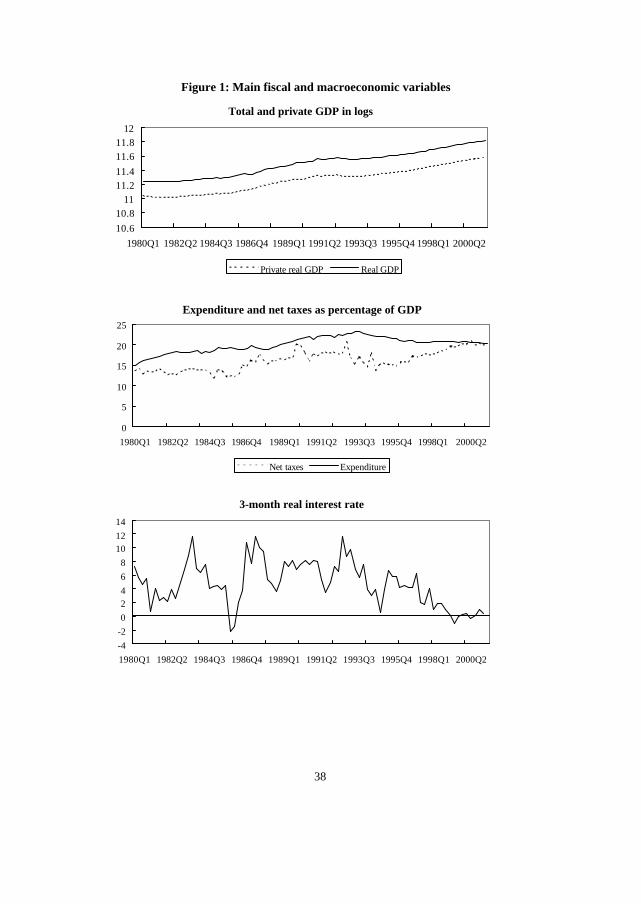
period 1980:1-2001:2. Figure 1 shows a general overview of the period.

2.2 The baseline VAR

The baseline VAR specification in its reduced form can be written as

t

k

iitit UYBCY ++= ∑

=−

1

(1)

1 These two variables have been constructed following Blanchard and Perotti (2002), Fatás and Mihov (2000) and Perotti (2002).

11

where Yt is the vector of endogenous variables (Gt, Rt, GDPt, Tt, Pt). The only deterministic

component is a constant term. Bi is the matrix of coefficients for the ith lag and Ut is the

vector containing the reduced form residuals, which in general will have non-zero

correlations. Equation (1) is estimated by OLS including five lags. The number of lags was

chosen according to the information provided by likelihood ratio tests and the Akaike

information criterion2.

Since the reduced form residuals have little economic significance in that they are

combinations of structural shocks, the identification of such structural components becomes

necessary. Var(U)=Σ is in general not diagonal because the reduced-form residuals are

combinations of the structural shocks. The innovation model can be written as

tt VAU = (2)

where Vt is the vector of the structural orthogonal shocks and DVVE tt =)'( with D

diagonal. Therefore, (2) can be expressed as

gt

pt

ntt

gdpt

rt

gt vuauauauau ++++= 5,14,13,12,1

rt

pt

ntt

gdpt

gt

rt vuauauauau ++++= 5,24,23,21,2

gdpt

pt

ntt

rt

gt

gdpt vuauauauau ++++= 5,34,32,31,3 (3)

ntt

pt

gdpt

rt

gt

ntt vuauauauau ++++= 5,43,42,41,4

pt

ntt

gdpt

rt

gt

pt vuauauauau ++++= 4,53,52,51,5

The system has been identified by using the Choleski decomposition with the order (Gt,

Rt, GDPt, Tt, Pt). Although there are many other alternatives, the arguments below aim at

providing some support to the scheme adopted.

The definition used for public expenditure allows for setting a1,2=a1,3= a1,4=a1,5=0. The

readings contained in Gt are assumed to be predetermined within the quarter with respect to

2 Admittedly, the number of lags seems a little bit awkward for quarterly data. However, given the information collected by the tests mentioned I preferred to set it accordingly. On the other hand, the VAR with four lags did not offer different results from those reported in this paper in terms of impulse responses or multipliers.

12

taxes, output, prices3 and interest rates. Before the reaction of the authorities to changes in

underlying economic conditions takes place, the situation has to be recognised and

assessed. In addition, the approval and implementation phases also take some time. Thus,

spending only depends contemporaneously on its own structural shock without being too

restrictive.

The interest rate is assumed to react with a certain delay to output and price

developments, in that these are not immediately observed. Moreover, the contemporaneous

response of the short-term interest rate to shocks to net taxes is also set to zero.

Consequently, the interest rate is only allowed to respond to expenditure shocks and its own

structural component within the quarter.

On the other hand, monetary policy shocks are assumed to affect output, net taxes and

prices within the same quarter since, in many cases, interest rate movements are anticipated

and their transmission to real variables is relatively fast. Although the hypothesis that

interest rate movements do not affect output and prices contemporaneously has been

extensively used in empirical work (Bernanke and Blinder, 1992, Bernanke and Mihov,

1998, and Christiano et al., 1999, among others), Perotti (2002) admits that “this

assumption is by no means uncontroversial”. Nevertheless, as section 3.3 shows, the bulk

of the results presented here do not seem to be very sensitive to this assumption.

Shocks to net taxes are assumed not to affect activity significantly within the quarter,

since consumption and investment plans take some time to be adapted to the new

conditions as agents will need some time to calibrate the effects of the shock. By contrast,

changes in activity are expected to affect tax collections, notably through personal income

tax withholdings, social security contributions and indirect taxes directly linked to final

consumption. Finally, prices will respond to movements in the rest of the variables of the

system and thus, all the coefficients in the price equation are freely estimated. The baseline

model then becomes

gt

gt vu =

rt

gt

rt vuau += 1,2

3 In any case, this constraint does not seem to be restrictive in the present case, since alternative models were estimated without it and the results obtained were broadly the same (see section 3.3 for further details).

13

gdpt

rt

gt

gdpt vuauau ++= 2,31,3 (3’)

ntt

gdpt

rt

gt

ntt vuauauau +++= 3,42,41,4

pt

ntt

gdpt

rt

gt

pt vuauauauau ++++= 4,53,52,51,5

With this set of restrictions the model is exactly identified. In order to test the sensitivity

of the results to different identification schemes other alternatives were tried. However, in

many cases they produced similar impulse-response functions (see section 3.3) to fiscal

policy shocks.

The identification scheme (3’), as far as government expenditure is concerned, is similar

to those adopted in Blanchard and Perotti (2002), Fatás and Mihov (2000) and Perotti

(2002), in that this variable is taken as predetermined within the quarter with respect to the

rest of the rest of the variables is the VAR. Specifically, Fatás and Mihov (2000) adopt an

identification of a similar system with respect to expenditure, since their sole concern

applies to the effects derived from shocks to this variable. Thus, they avoid modelling the

contemporaneous relationships between net taxes and the rest of the variables in the system.

The rest of the contemporaneous interactions are left unrestricted in the tradition of semi-

structural VAR literature4.

Blanchard and Perotti (2002) analyse the effects of fiscal policy on activity by specifying

a three-variable baseline VAR5. Their methodology is based on the fact that unexpected

net-tax movements are due to their own structural shock and to the unexpected output

responses measured by the GDP reduced-form residuals. The latter are identified through

estimated GDP elasticities of different components of revenues. The identification of GDP

shocks is then achieved by instrumental variables estimation of the elasticities of GDP

reduced form residuals to the structural shocks of expenditure and net taxes. The remaining

residual is taken as the structural shock of output. Perotti (2002) extends this methodology

and includes prices and the 3-month interest rate in the VAR. However, he argues that real

spending should be affected by price shocks within the quarter, in that some spending

programmes are fixed in nominal terms while others are indexed to price developments,

4 See Bernanke and Blinder (1992) and Bernanke and Mihov (1998) for an application to the study of monetary policy shocks. 5 They include neither interest rate nor prices in the VAR.

14

although in the latter case indexation occurs with a considerable lag. Consequently, he

imposes a non-zero price elasticity of real government expenditure.

Marcellino (2002) uses revenues and expenditure to GDP ratios as fiscal variables.

Therefore, the restrictions imposed to identify the VAR have, in this respect, to be different.

Namely, the disbursements-to-GDP ratio is related to contemporaneous values of the output

gap and interest rate.

As explained above, real net taxes are affected by output, expenditure and interest rates

within the quarter. This can also be found in Blanchard and Perotti (2002) and Perotti

(2002). However, they use external information to compute the output elasticities of

different tax-categories. Accordingly, the approach followed here is closer, in this respect,

to that in Marcellino (2002).

Finally, it is worth noting that in the model monetary policy is treated differently from

fiscal policy. Monetary policy shocks take place when the decision of shifting interest rates

is adopted. This is not the case for fiscal policy. The decision to undertake a given

expenditure programme can be announced at a certain point in time. However, the

programme has to be evaluated and its implementation takes some time. Therefore, there

are considerable lags between the period in which it has been decided to undertake an

expenditure programme and its implementation, typically several quarters. Moreover, the

data only reflect the policy measure once the expenditure has been recognised as a liability,

but not before, when the measure was really approved. However, it is precisely at this stage

when we should quantify the effect of a given measure since it is expected to have been

incorporated in agents’ expectations and thus be affecting their decisions. Unfortunately,

the lack of data of such characteristics does not permit assessment fully in depth of the

effects of fiscal policy, at least under this framework, and obliges to take the results with

care.

3 Empirical results

In this section the impulse-response functions and multipliers derived from fiscal shocks

are presented. In all cases, impulse responses are reported for five years and the one-

standard deviation confidence bands have been obtained by Monte Carlo integration

methods with 100 replications.

15

Table 1 shows the variance decomposition of the baseline model. Both fiscal variables

play a crucial role in explaining each other. The forecast error of Gt forty quarters ahead is

mainly explained by itself, by above 60%, whereas net taxes explain a significant share

above 20% and GDP shocks come to explain around 11%. Net taxes are mainly explained

by their own shocks (37.8%), expenditure (36.6%) and output shocks (18%). Regarding

GDP, again shocks to spending (40%), net taxes (22.5%) and GDP itself (33.3%) explain

the biggest share. Although surprising, the high share of variance of output explained by

shocks to government expenditure could be due to the increasing spending-to-GDP ratio

until 1993, linked to the building up of the Welfare State. The same argument applies for

net taxes. Nevertheless, this issue deserves further research. Shocks to interest rate and

prices only seem to play a prominent role in explaining their own forecast errors.

Table 1: Variance decomposition in the baseline VAR

Percentage of the forecast error of:

Quarters

Explained by shocks in:

G R GDP T P G 4 91.14 0.04 1.86 6.09 8.87 8 82.46 0.16 2.39 13.41 1.58 12 73.46 0.15 4.18 19.56 2.65 16 67.61 0.41 7.55 20.40 4.02 20 64.11 1.06 10.38 20.04 4.41 40 61.25 1.55 11.00 22.31 3.89

R 4 24.23 68.61 0.51 5.74 0.91 8 32.84 51.19 0.60 7.37 8.00 12 39.95 42.00 1.27 9.80 6.98 16 40.13 39.54 1.35 12.38 6.60 20 39.77 38.12 1.37 13.96 6.77 40 39.88 37.35 1.79 14.20 6.78

GDP 4 14.15 1.60 81.40 2.57 0.28 8 11.75 4.23 76.44 6.99 0.59 12 8.77 5.41 79.93 4.98 0.91 16 14.26 5.93 73.84 5.23 0.74 20 24.51 5.54 60.42 8.98 0.55 40 40.07 3.57 33.30 22.53 0.53

T 4 17.15 5.45 11.07 66.09 0.24 8 20.41 4.82 17.75 51.56 5.46 12 18.78 6.80 24.51 45.21 4.70 16 20.84 6.91 26.47 41.47 4.31 20 26.49 6.17 25.28 38.32 3.74 40 36.61 4.57 18.00 37.81 3.01

P 4 3.67 0.18 1.28 14.78 80.09 8 15.33 2.64 2.08 13.81 66.14 12 26.77 4.31 1.75 10.76 56.41 16 36.99 3.35 2.42 8.48 48.76 20 43.50 2.75 3.86 7.56 42.33 40 42.64 3.90 11.82 6.20 35.44

16

3.1 The effects of government spending

Figure 2 shows the responses of the endogenous variables to a one-standard deviation

shock to government expenditure. This shock is remarkably persistent, with seventy per

cent of the shock still present after three years, declining thereafter. The effect on GDP is

positive and significant during the first six quarters, with the peak effect in the fourth

quarter at around 0.29%6. Afterwards, it declines steadily and becomes negative and

significant after the 13th quarter.

Following the behaviour of output, net taxes respond recording a significant increase

during almost the first two years, also reaching their peak response in the fourth quarter.

The response of net taxes can partially be explained by the positive response of output and

partly to a reaction of the authorities to financing the increasing expenditure. After the

second year, they decline and this fall becomes significant after 15 quarters. As a result of

the reaction of taxes the budget balance hardly responds during the first two years, which is

somewhat counterintuitive. In the third year, however, a persistent deficit arises.

Prices fall on impact but increase steadily after the third quarter, with the peak response

in the fifth year. This effect is very persistent and also quite intuitive. Nevertheless, it

contrasts with the evidence presented by Fatás and Mihov (2000) for the US and Marcellino

(2002), who find negative price effects after a government expenditure shock. Finally,

nominal and real interest rates rise persistently.

Table 2: Cumulative output multipliers to a government expenditure shock

Quarters

Shock to: 4th q 8th q 12th q 16th q 20th q

Expenditure (Baseline VAR) 1.14 1.04 0.58 -0.05 -0.83

Expenditure

(VAR with long term rates)

1.54

1.55

1.04

0.50

-0.10

The table shows the cumulative multipliers to a one-standard deviation shock to government spending. The baseline VAR contains five variables: Gt, Rt, GDPt, Tt and Pt.

17

The cumulative output multipliers7 to spending shocks are presented in Table 2. These

are slightly above one in the first two years, 1.14 and 1.04 in the fourth and eighth quarters

after the shock respectively, and turn to negative from the 16th quarter onwards.

Since consumption and investment decisions are more closely related to the evolution of

medium or long-term real interest rates, a VAR including bank loan rates with a maturity of

three years or more was estimated. The pattern of responses was similar although the

effects on GDP turned out to be larger, with the cumulative multipliers at around 1.55 in the

first and second year8. On the other hand, long-term rates pose additional drawbacks at the

identification stage in that they are strongly influenced by more permanent and structural

factors. Therefore, the underlying reason behind the choice of the short-term interest rate is

that it basically includes monetary policy decisions and not so much expectations,

facilitating identification.

The short-term multipliers shown here are in line with those found in Willman and

Estrada (2002) with a large-scale macroeconometric model for the Spanish economy, in

that they obtain a multiplier at around 1.25 and 1.40 in the first and second year

respectively, after a shock to public consumption. The negative medium-term values,

however, are in line with those in Perotti (2002).

3.2 The effects of net taxes

Figure 3 shows the responses following an increase of net taxes. Around 85% of the initial

shock disappears after four quarters, although remains significant until the end of the

second year. The response keeps on declining thereafter, becoming negative and only

marginally significant in the fifth year. Government spending falls in the quarter following

the shock, although increasing immediately afterwards to reach its peak in the 10th quarter.

The response of spending is very persistent and remains significant for four years, which

leads to a permanent deficit in the medium term. This provides further support to the

6 Fatás and Mihov (2000) find effects of a similar magnitude for the US economy, although reaching the peak takes more time. 7 The cumulative dynamic multiplier at a given quarter is obtained as the ratio of the cumulative response of GDP and the cumulative response of government expenditure. 8 The corresponding impulse responses are not presented for brevity reasons.

18

hypothesis of the existence of a bias towards deficit in the public sector size (De Castro et

al., 2002).

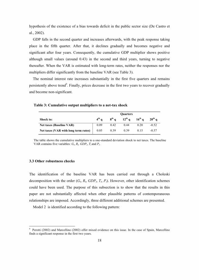
GDP falls in the second quarter and increases afterwards, with the peak response taking

place in the fifth quarter. After that, it declines gradually and becomes negative and

significant after four years. Consequently, the cumulative GDP multiplier shows positive

although small values (around 0.43) in the second and third years, turning to negative

thereafter. When the VAR is estimated with long-term rates, neither the responses nor the

multipliers differ significantly from the baseline VAR (see Table 3).

The nominal interest rate increases substantially in the first five quarters and remains

persistently above trend9. Finally, prices decrease in the first two years to recover gradually

and become non-significant.

Table 3: Cumulative output multipliers to a net-tax shock

Quarters


Net taxes (Baseline VAR) 0.09 0.42 0.44 0.20 -0.52

Net taxes (VAR with long term rates) 0.05 0.39 0.39 0.15 -0.57

The table shows the cumulative multipliers to a one-standard deviation shock to net taxes. The baseline VAR contains five variables: Gt, Rt, GDPt, Tt and Pt.

3.3 Other robustness checks

The identification of the baseline VAR has been carried out through a Choleski

decomposition with the order (Gt, Rt, GDPt, Tt, Pt). However, other identification schemes

could have been used. The purpose of this subsection is to show that the results in this

paper are not substantially affected when other plausible patterns of contemporaneous

relationships are imposed. Accordingly, three different additional schemes are presented.

Model 2 is identified according to the following pattern:

9 Perotti (2002) and Marcellino (2002) offer mixed evidence on this issue. In the case of Spain, Marcellino finds a significant response in the first two years.

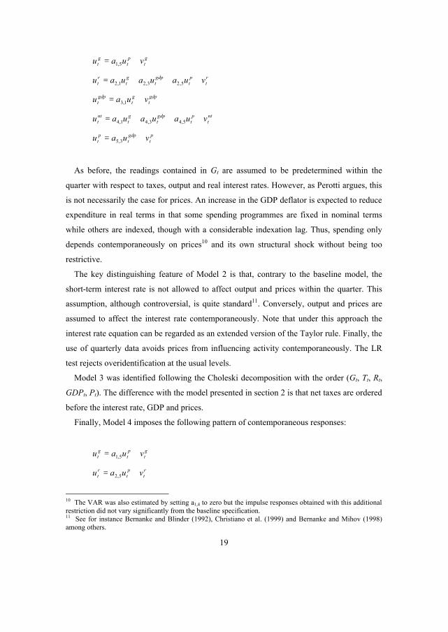
19

gt

pt

gt vuau += 5,1

rt

pt

gdpt

gt

rt vuauauau +++= 5,23,21,2

gdpt

gt

gdpt vuau += 1,3

ntt

pt

gdpt

gt

ntt vuauauau +++= 5,43,41,4

pt

gdpt

pt vuau += 3,5

As before, the readings contained in Gt are assumed to be predetermined within the

quarter with respect to taxes, output and real interest rates. However, as Perotti argues, this

is not necessarily the case for prices. An increase in the GDP deflator is expected to reduce

expenditure in real terms in that some spending programmes are fixed in nominal terms

while others are indexed, though with a considerable indexation lag. Thus, spending only

depends contemporaneously on prices10 and its own structural shock without being too

restrictive.

The key distinguishing feature of Model 2 is that, contrary to the baseline model, the

short-term interest rate is not allowed to affect output and prices within the quarter. This

assumption, although controversial, is quite standard11. Conversely, output and prices are

assumed to affect the interest rate contemporaneously. Note that under this approach the

interest rate equation can be regarded as an extended version of the Taylor rule. Finally, the

use of quarterly data avoids prices from influencing activity contemporaneously. The LR

test rejects overidentification at the usual levels.

Model 3 was identified following the Choleski decomposition with the order (Gt, Tt, Rt,

GDPt, Pt). The difference with the model presented in section 2 is that net taxes are ordered

before the interest rate, GDP and prices.

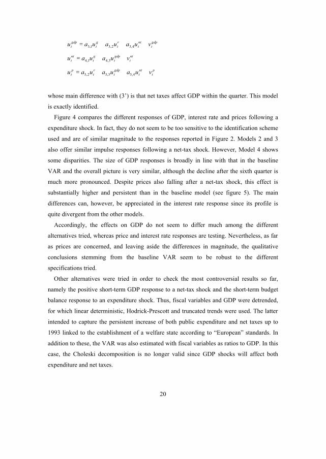
Finally, Model 4 imposes the following pattern of contemporaneous responses:

gt

pt

gt vuau += 5,1

rt

pt

rt vuau += 5,2

10 The VAR was also estimated by setting a1,4 to zero but the impulse responses obtained with this additional restriction did not vary significantly from the baseline specification. 11 See for instance Bernanke and Blinder (1992), Christiano et al. (1999) and Bernanke and Mihov (1998) among others.

20

gdpt

ntt

rt

gt

gdpt vuauauau +++= 4,32,31,3

ntt

gdpt

gt

ntt vuauau ++= 3,41,4

pt

ntt

gdpt

rt

pt vuauauau +++= 4,53,52,5

whose main difference with (3’) is that net taxes affect GDP within the quarter. This model

is exactly identified.

Figure 4 compares the different responses of GDP, interest rate and prices following a

expenditure shock. In fact, they do not seem to be too sensitive to the identification scheme

used and are of similar magnitude to the responses reported in Figure 2. Models 2 and 3

also offer similar impulse responses following a net-tax shock. However, Model 4 shows

some disparities. The size of GDP responses is broadly in line with that in the baseline

VAR and the overall picture is very similar, although the decline after the sixth quarter is

much more pronounced. Despite prices also falling after a net-tax shock, this effect is

substantially higher and persistent than in the baseline model (see figure 5). The main

differences can, however, be appreciated in the interest rate response since its profile is

quite divergent from the other models.

Accordingly, the effects on GDP do not seem to differ much among the different

alternatives tried, whereas price and interest rate responses are testing. Nevertheless, as far

as prices are concerned, and leaving aside the differences in magnitude, the qualitative

conclusions stemming from the baseline VAR seem to be robust to the different

specifications tried.

Other alternatives were tried in order to check the most controversial results so far,

namely the positive short-term GDP response to a net-tax shock and the short-term budget

balance response to an expenditure shock. Thus, fiscal variables and GDP were detrended,

for which linear deterministic, Hodrick-Prescott and truncated trends were used. The latter

intended to capture the persistent increase of both public expenditure and net taxes up to

1993 linked to the establishment of a welfare state according to “European” standards. In

addition to these, the VAR was also estimated with fiscal variables as ratios to GDP. In this

case, the Choleski decomposition is no longer valid since GDP shocks will affect both

expenditure and net taxes.

21

None of these alternatives produced results very different from those already reported. In

fact, expenditure shocks lead to significantly increased prices, interest rates and net taxes.

Moreover, GDP always increased in the short term and tended to fall after some quarters.

Shocks to net taxes reduced prices and in all cases led expenditure and short-term output

upwards. Moreover, shocks to net taxes always showed a lower degree of persistence than

shocks to public expenditure.

3.4 Effects on consumption and investment

In order to account for the responses of private consumption and private investment a 6

variable VAR was estimated (Gt, Rt, Xt, GDPt, Tt, Pt), where Xt is the new variable that is

added in turn to the VAR. The decision to analyse the responses of private consumption or

private investment is self-explanatory because of their share in GDP.

The identification is again carried out by using the Choleski decomposition12 with the

order (Gt, Rt, Xt, GDPt, Tt, Pt). Thus, the imposed pattern of contemporaneous relationships

was:

gt

gt vu =

rt

gt

rt vuau += 1,2

xt

rt

gt

xt vuauau ++= 2,31,3

gdpt

xt

rt

gt

gdpt vuauauau +++= 3,42,41,4 (4)

ntt

gdpt

xt

rt

gt

ntt vuauauauau ++++= 4,53,52,51,5

pt

ntt

gdpt

xt

rt

gt

pt vuauauauauau +++++= 5,64,63,62,61,6

Private consumption and investment react contemporaneously to shocks to government

spending13 and the interest rate. As they are components of output, shocks to consumption

or investment affect GDP contemporaneously. For the same reasons as in the case of GDP,

the Xt component is allowed to affect net taxes and prices within the quarter. Figure 6 shows

12 As in the GDP case, some alternative schemes were tried and all yielded results very similar to the ones reported in this paper.

22

the impulse response functions of private consumption and investment to both government

expenditure and net-tax shocks.

Responses to a shock on government spending

Private consumption reproduces the pattern of GDP and increases steeply until it reaches its

peak in the fourth quarter at around 0.35%. After that, it declines gradually to become

negative and significant in the fifth year.

Private investment falls slightly on impact but increases in the second quarter, reaching

its peak in the third at around 1.1% and remaining positive and significant until the seventh

quarter. Then, it begins to decline and becomes negative and significant from the 14th

quarter onwards. The multipliers presented in Table 4 show values above one in the second

year after the shock in both cases. In the medium term the investment multiplier is

substantially lower than the consumption multiplier. The estimation of the VAR with long-

term rates somewhat inflates the multipliers, more pronouncedly in the case of private

investment, although the profile remains broadly unchanged.

Responses to a shock on net taxes

Following an increase in net taxes, real private consumption rises to reach its peak in the

fourth quarter, remaining significant until the 10th quarter after the shock. Then, it starts to

decline, becoming negative, although non-significant.

Investment falls in the third quarter and then jumps briskly to reach its peak in the fifth

one, declining thereafter and becoming negative and significant in the fifth year. The

multipliers in Table 4 are positive for both GDP components (around 0.6 in the 12th

quarter). However, when the VAR is estimated with long-term real interest rates the

cumulative investment multipliers become considerably lower and negative in the fifth

year. The fact that long-term rates incorporate a non-negligible content of expectations may

be behind this result.

The patterns of response for consumption and investment are quite unexpected, though in

accordance with the effects observed in output. However, the increase in government

expenditure in response to an increase in taxes may be playing a prominent role.

13 Some components of government expenditure are value added produced by the private sector. Thus, a shock in this variable is automatically reflected in disposable income of households and enterprises, which is expected to influence consumption or investment.

23

Table 4: Cumulative multipliers of GDP components

Shock to government expenditure

Quarters

Response of: 4th q 8th q 12th q 16th q 20th q

Private consumption 0.91 1.20 0.98 0.64 0.26

Private consumption


0.80

1.26

1.17

0.95

0.75

Private investment 0.93 1.18 0.79 0.19 -0.33

Private investment


1.51

1.76

1.28

0.77

0.34

Shock to net taxes

Quarters

Response of: 4th q 8th q 12th q 16th q 20th q

Private consumption 0.27 0.49 0.65 0.70 0.60

Private consumption


0.17

0.34

0.52

0.58

0.53

Private investment 0.02 0.57 0.60 0.53 0.26

Private investment


-0.19

0.10

0.05

0.01

-0.29

The table shows the cumulative multipliers to a one-standard deviation shock to government expenditure and net taxes. The VAR contains six variables: Gt, GDPt, Tt, Rt, Pt and the indicated GDP component.

3.5 Effects of changes in government spending components

Following Fatás and Mihov (2000), this subsection aims at comparing the responses of the

key macroeconomic variables considered in this paper to shocks to the different

components of public spending. Thus, the responses to increases in a) purchases of goods

and services (Figure 7), b) compensation of civil servants (Figure 8) and c) public

24

investment (Figure 9) are studied. In order to carry out the analysis, the aggregate

expenditure variable is replaced by the component14 in turn in models (3’) and (4).

The induced responses to a shock to these three components are very different. After the

initial shock, the response of purchases of goods and services shows little persistence and

disappears in the early quarters, becoming non-significant. Following the initial increase,

the response of compensation of civil servants moderates gradually, being significant

during the first two years. Finally, the response of public investment is positive and

significant until the 10th quarter. It shows a higher degree of persistence than the other

spending components.

GDP increases in the first quarters after a shock on public investment15, with the peak

response in the fourth quarter. The response becomes non-significant at the end of the

second year. On the contrary, the GDP response after a shock to purchases of goods and

services is, in general, non-significant in the short term and becomes significant and

negative in the fifth year after the shock. The multipliers in table 5 show that public

investment seems to be more efficient than public consumption items in stimulating

economic activity. This result is in accordance with Baxter and King (1993) and Marcellino

(2002) in the case of Spain. The responses of private consumption and investment show

similar profiles in both cases, increasing in the first quarters after the shock and falling in

the medium term. Contrary to the other spending readings, a shock to compensation of civil

servants reduces output persistently. This pattern is also reproduced in private consumption

and investment. A possible explanation for such effects can be found in Alesina et al.

(1999). In all cases, as expected, the response of net taxes broadly mimics GDP or private

consumption’s profiles.

14 This is the approach adopted by Fatás and Mihov (2000). It could be argued that omitting the rest of the components of public expenditure, once recognised they are important in affecting other macro-variables, might bias the results. However, this is no longer the case here since models that included both total expenditure and the specific component in turn were also estimated and the results were very similar to those presented in this paper, although the estimates were more imprecise. Given the low number of observations compared with the large number of coefficients in the VAR, it made sense to reduce the VAR dimension. The same applies for the case of net taxes’ components.

25

Table 5: Cumulative output multipliers to shocks on spending components

Quarters


Expenditure on goods and services 1.46 2.15 -0.73 -5.40 -14.14

Expenditure on compensation of civil

servants

-0.84

-2.79

-5.71

-10.58

-20.15

Expenditure on public investment 2.42 3.40 3.30 2.37 1.35

The table shows the cumulative multipliers to a one-standard deviation shock to government spending. The baseline VAR contains five variables: SCt, Rt, GDPt, Tt and Pt, where SC is the relevant spending component.

3.6 Effects of changes in components of net taxes

There is a large body of theoretical work on the different economic effects of direct and

indirect taxation. In this subsection the responses of the variables under analysis to shocks

on both types of taxation will be briefly studied.

A shock to indirect taxes shows little persistence and becomes non-significant after two

quarters (see Figure 10). This shock reduces GDP, private consumption and investment.

The reduction is, in all cases, sizeable and significant in the first three years (Table 6 shows

the cumulative output multiplier, which records –3.9 in the 12th quarter). Surprisingly,

public expenditure contracts.

The shock to direct taxes (Figure 11) disappears more gradually than the shock to

indirect taxes. The responses of GDP and private consumption are positive and significant

in the first five quarters, although these become negative in the medium term. The

cumulative multipliers in Table 6 show low, though positive, values until the fourth year. In

any case, direct-tax shocks do not appear to have big effects on activity in the short term

and the expected negative effects arise in the medium term.

In sum, shocks to indirect taxation seem to be clearly contractionary, whereas shocks to

direct taxation do not seem to affect activity significantly in the short term. However, it

must be stressed that the different effects stemming from shocks to indirect and direct taxes

15 Nevertheless, the estimations in this paper might not fully account for the effects of public investment, since some investment programmes with important spillover effects are carried out by State-owned entities not included in the general government accounts according to ESA-95 definitions.

26

are counterintuitive. In principle, one would expect increases in direct taxes to have a more

negative impact on activity than indirect taxes. In addition, the divergent behaviour of

expenditure following the shock is at least striking. Notably, the fall of spending in

response to an indirect-tax shock turns out to be unexpected and no straightforward

explanation is found for it, while the response to a direct-tax shock is in accordance to the

findings in section 3.2 for the baseline VAR.

Table 6: Cumulative output multipliers to shocks on net-tax components

Quarters


Indirect taxes -2.28 -3.22 -3.90 -3.81 -3.16

Direct taxes 0.21 0.44 0.04 -0.81 -2.19

The table shows the cumulative multipliers to a one-standard deviation shock to net taxes. The baseline VAR contains five variables: Gt, Rt, GDPt, TCt and Pt, where TC is the relevant net-tax component.

3.7 The experience of the 1990s

In the recent years a change in the fiscal policy regime seems to have taken place16. A quite

remarkable spending-side oriented consolidation process has been carried out, encouraged

by the Maastricht Treaty criteria and the Stability and Growth Pact. It has been claimed that

expenditure-based fiscal consolidations could, under certain circumstances, involve low

costs in terms of output and employment even in the short term. Moreover, in some

countries with a poor reputation for fiscal discipline and high levels of public debt, credible

spending-oriented consolidation programmes could even be expansionary, in that they

could help to create a more stable macroeconomic framework by reducing real interest

rates. Alesina and Ardagna (1998) Alesina et al. (1999) and Von Hagen et al. (2001) find

evidence along these lines.

The purpose of this sub-section is to assess whether the consolidation process has

involved real costs. Thus, the sample was restricted to the period since 1992 onwards to

estimate again the baseline VAR (3’). Notwithstanding output multipliers to public

16 De Castro and Hernandez de Cos (2002) provide empirical evidence on this statement.

27

expenditure being higher than for the whole sample17 (see Table 7), the GDP response is

broadly non-significant, as Figure 12 shows. In addition, nominal interest rate responses are

not significant either, in line with the findings in Von Hagen et al. (2001). The low

magnitude of the responses and the less persistence shown by fiscal shocks seem to be

behind these results and, in comparison with the whole sample, might reflect a shift in the

fiscal policy regime. This also applies to net-tax shocks that also yield non-significant and

almost null GDP responses.

Therefore, these pieces of empirical evidence might suggest that the consolidation

process in Spain has not involved significant real costs. In fact, some quarters highlight the

positive effects stemming from the consolidation process18 and argue that helping to create

greater macroeconomic stability, the traditional effects of fiscal policy could be offset by

those derived from the improved expectations. In this respect, lower real rates and inflation

in the future, coupled with lower taxes, might ensure higher sustainable growth in the long

term. However, the small number of observations obliges one to view these results with

caution.

Table 7: Cumulative output multipliers (sample 1992Q1-2001Q2)

Quarters


Expenditure 1.83 1.48 1.50 1.84 1.36

Net taxes 0.21 0.29 -0.11 0.24 -0.24

The VAR contains five variables: Gt, Rt, GDPt, Tt and Pt.

17 This outcome might, in principle, be consistent with the higher effectiveness of fiscal policy under fixed exchange rate regimes. 18 Although not explicitly mentioned, the explanatory memorandum to the Budgetary Stability Law, approved in Spain at the end of 2001, makes an explicit recognition of the benefits of continuing further with the consolidation strategy in guaranteeing a greater macroeconomic stability and accordingly a stable framework for higher and sustained growth in the future. González-Páramo (2001) shows a useful discussion on the effects stemming from the consolidation process in Spain.

28

4 Assessment of the results

As noted in the introduction, there are not yet many pieces of empirical literature on the

effects of fiscal policy. However, in order to provide some perspective, the evidence

presented here can be compared with some recent studies already mentioned in this paper.

In addition, some of the results in this paper deserve further comment.

4.1 Government expenditure

One of the most remarkable features of the current study is that following a shock to

government expenditure real output and consumption increase in the first two years and

decline thereafter. While the short-term multipliers are in line with the results obtained by

Willman and Estrada (2002) for Spain, the negative medium-term values contrast with their

findings. On the other hand, GDP and consumption profiles are in accordance with those

obtained by Perotti (2002) in the cases of the USA, Germany, Canada and the United

Kingdom when he restricts the sample period to 1980 onwards. In contrast, the multipliers

he calculates are significantly lower than those reported here and typically below one in the

short term, whereas his the medium-term negative multipliers are in line with those in

Table 2. On the other hand, Edelberg et al. (1998), Blanchard and Perotti (2002), Burnside

et al. (1999) and Fatás and Mihov (2000) show that GDP rises persistently after an

expenditure shock in the US. Mountford and Uhlig (2002) also present positive GDP and

consumption responses in the first two years although again with low multipliers, in line

with the values obtained here.

Private investment profiles are similar to those of GDP and consumption, showing a

close connection between investment and activity, in accordance with the accelerator

hypothesis. Investment responses are in line with the mixed evidence across countries

found by Perotti. For this variable, Blanchard and Perotti and Mountford and Uhlig find a

negative effect after a spending shock, whereas Fatás and Mihov detect effects of the

opposite sign. Edelberg et al. (1998) distinguish between residential and non-residential

investment, obtaining negative responses in the former case and positive in the latter.

29

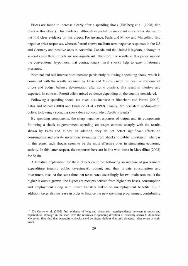
Prices are found to increase clearly after a spending shock (Edelberg et al. (1998) also

observe this effect). This evidence, although expected, is important since other studies do

not find clear evidence on this aspect. For instance, Fatás and Mihov and Marcellino find

negative price responses, whereas Perotti shows medium-term negative responses in the US

and Germany and positive ones in Australia, Canada and the United Kingdom, although in

several cases these effects are non-significant. Therefore, the results in this paper support

the conventional hypothesis that contractionary fiscal shocks help to ease inflationary

pressures.

Nominal and real interest rates increase persistently following a spending shock, which is

consistent with the results obtained by Fatás and Mihov. Given the positive response of

prices and budget balance deterioration after some quarters, this result is intuitive and

expected. In contrast, Perotti offers mixed evidence depending on the country considered.

Following a spending shock, net taxes also increase in Blanchard and Perotti (2002),

Fatás and Mihov (2000) and Burnside et al. (1999). Finally, the persistent medium-term

deficit following a spending shock does not contradict Perotti’s results19.

By spending components, the sharp negative responses of output and its components

following a shock to government spending on wages contrast sharply with the results

shown by Fatás and Mihov. In addition, they do not detect significant effects on

consumption and private investment stemming from shocks to public investment, whereas

in this paper such shocks seem to be the most effective ones in stimulating economic

activity. In this latter respect, the responses here are in line with those in Marcellino (2002)

for Spain.

A tentative explanation for these effects could be: following an increase of government

expenditure (mainly public investment), output, and thus private consumption and

investment, rise. At the same time, net taxes react accordingly for two main reasons: i) the

higher is output growth, the higher are receipts derived from higher tax bases, consumption

and employment along with lower transfers linked to unemployment benefits. ii) in

addition, taxes also increase in order to finance the new spending programmes, contributing

19 De Castro et al. (2002) find evidence of long and short-term interdependence between revenues and expenditure, although in the short term the revenues-to-spending direction of causality seems to dominate. Moreover, they find that expenditure shocks yield persistent deficits that only disappear after seven or eight years.

30

to moderate the response of output. The response of net taxes offsets the higher

expenditure, leaving the budget balance barely changed in the first quarters.

As a result of higher demand pressures, prices and interest rates increase persistently.

The interest response could have a double component regarding the time-horizon. Notably,

the endogenous response of monetary policy in the short term to higher inflation would lead

rates upwards, whereas in the medium term the higher persistent deficits would bring about

additional pressures on debt markets.

The higher real interest rates, reinforced by the phasing out response of public

expenditure would help slow down activity mainly through their effects on investment,

stemming from higher discount rates and user cost of capital. Moreover, higher inflation

would erode competitiveness, undermining potential and effective growth in the medium

term.

Although in the short term these facts seem in principle to fit well the traditional

Keynesian predictions summarised by the standard IS-LM textbook model, the negative

medium-term output multipliers could be due to both the higher interest rates and wage

claims as a result of higher inflation, contributing to reduce entrepreneurial profits and thus

investment (Alesina et al., 1999). This interpretation would be consistent with the negative

response of activity observed after a shock to the government wage bill. According to this

view, fiscal consolidations can even be expansionary due to the better prospects envisaged

by private economic agents (see Von Hagen et al., 2001).

Despite the interest of some results, some caveats should be highlighted. First, fact that

the endogenous response of net taxes leaves the budget balance barely affected in the first

quarters, turns out to be quite counterintuitive and contradicts the results obtained by other

authors. This might stem from two potential sources: On the one hand, quarterly Spanish

fiscal data have been constructed by using a set of indicators, but they do not correspond to

official observed series. In addition, the history of fiscal policy in Spain is somewhat

different from other countries in that the 1980s and early 1990s were characterised by

rapidly increasing public expenditure and revenues associated with the building of the

Welfare State20 following the political change that took place in the second half of the

1970s. This factor could help explain the high share of the variance of output explained by

20 Argimón et al. (1999) provide a detailed description of the evolution of the general government sector in Spain.

31

shocks to government expenditure and might be conditioning the responses observed in

some variables, particularly net taxes. Furthermore, the bulk of spending and tax measures

are decided jointly on an annual basis. Quarterly data do not properly reflect this issue and

obliges to take the results with care. This criticism would also apply to most of the studies

previously mentioned.

Another factor, however, should not be disregarded: in the identified VAR a theoretical

structure linking taxes and output is not imposed, which in principle is the most

controversial issue as far as the identification is concerned. In this respect, Blanchard and

Perotti (2002) constitute an important reference for further research in this field that could

help clarify some aspects of the current paper. This will be left for future work.

4.2 Net taxes

Another striking feature of the current results is that GDP, private consumption and

investment increase in the first few quarters following a shock to net taxes. Although

contrasting sharply with Blanchard and Perotti and Mountford and Uhlig, these short-term

positive responses can also be found in Australia, the USA and the United Kingdom in

Perotti (2002). Moreover, Marcellino (2002) shows that the output gap increases in the

short term in Spain, Italy and France. As pointed out above, Alesina et al. (1999) and Von

Hagen et al. (2001) provide theoretical arguments and empirical evidence on such effects.

They claim that under some specific circumstances such as high or rapidly increasing debt-

to-GDP ratios, fiscal consolidations may have an expansionary effect even in the short term

due to expected lower deficits. Accordingly, higher taxes would lead agents to expect lower

interest rates derived from the consolidation process. The medium-term negative responses,

however, are in accordance with the other studies.

The negative response of prices can only be compared with the papers by Perotti (2002)

and Marcellino (2002). While the former finds mixed evidence across countries Marcellino

obtains non-significant inflation responses in any of the cases considered. However,

regarding the increase of nominal and real interest rates there is greater accord between

Perotti’s and the results shown here. In turn, a similar pattern of response is found by

Marcellino in Spain.

32

The increase in net taxes would lead output and prices to decrease. In this respect,

consumers’ permanent income would decline, although consumption plans take some time

to be adapted to the new situation. On the other hand, public expenditure increases21,

fuelling activity. Thus, the short-term positive reaction of output would stem from the

endogenous increase of public expenditure, whereas the lower permanent income following

a tax shock would lead consumption down in the medium term. In addition, higher taxes,

especially on labour, would reduce the profitability of investment projects and

entrepreneurial profits, discouraging investment in the medium term. This effect would be

reinforced by the loss of efficiency derived from higher taxation.

The budget balance deterioration in the medium term (Perotti also observes this effect in

Germany) as a result of the reaction of government expenditure was, however, to some

extent expected. In this regard, De Castro et al. (2002) detect a bias towards deficit in the

public sector’s size. Accordingly, the interest rate rises permanently due to higher pressure

on debt markets.

So far, the short-term responses do not fit the Keynesian paradigm, since it predicts

different signs for the output responses to spending and tax shocks. However, this paper

shows that in both cases output moves in the same direction in the quarters following the

shock. In this respect, the endogenous response of fiscal variables seems to play a role in

explaining these signs.

As stated above, the short-term positive output responses to a net-tax shock is a result

already obtained by other authors. Despite some theoretical support provided by Alesina et

al. (1999), this result is quite unexpected. In this respect, the caveats highlighted in the

previous sub-section apply here.

In addition, no convincing explanation has been found for the different effects stemming

from shocks to direct and indirect taxes. They could be due to the identification scheme

used. It remains to be checked whether more institutional-based approaches like those used

in Perotti (2002) or Blanchard and Perotti (2002) would offer different conclusions.

21 Brennan and Buchanan (1980), Friedman (1978) and Gramlich (1989), among others, offer theoretical explanations for this behaviour.

33

5 Concluding remarks

This paper aims at investigating the effects of fiscal policy in Spain. Shocks to government

expenditure boost GDP, private consumption and investment, with multipliers close to one

in the short term and negative in the medium and long term. The inclusion of long-term real

interest rates in the VAR increases the magnitude of the responses but in no case do short-

term GDP multipliers breach 1.6. Despite this, the negative effects after expenditure build-

ups in the long term remain. Increases of net taxes also lead GDP, consumption and

investment upwards although the multipliers are below 0.45 in the short term and negative,

as expected, in the medium term. The inclusion of long-term real rates reduces multipliers

only slightly. As far as prices are concerned, real interest rates increase persistently after a

shock to either spending or net taxes, while the GDP deflator rises following a shock to

spending (in contrast with the evidence presented by Fatás and Mihov (2000) for the US)

and declines after a shock to net taxes.

So far the results obtained do not fit the Keynesian view that would predict different

signs for the output response to shocks to spending and taxes. In this respect, the

endogenous response of fiscal variables to both sources of shocks seems to play a role in

explaining output movements. Moreover, shocks to government expenditure are followed

in turn by net taxes and vice-versa, yielding in both cases higher deficits in the medium

term. This supports the hypothesis of the existence of a bias towards deficit in the public

sector size. Furthermore, the negative medium-term output multipliers to spending shocks

constitutes, to some extent, a surprising result which might be explained either by the

persistent increase of the real interest rate or by the higher wage pressures reducing

investment profitability.

It is worth noting, however, that spending programmes and tax amendments are

approved, and thus incorporated in agents’ expectations, well in advance of their being

reflected in public accounts. In addition, they are jointly decided on an annual basis.

Therefore, it is possible that consumption and investment decisions have accounted for

these measures before they are implemented. Accordingly, the multipliers obtained by this

approach would be, to some extent, downward biased. However, the lack of consistent data

makes overcoming this problem difficult in practice.

34

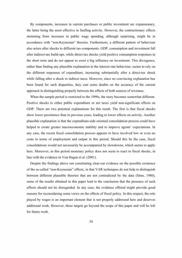
By components, increases in current purchases or public investment are expansionary,

the latter being the most effective in fuelling activity. However, the contractionary effects

stemming from increases in public wage spending, although surprising, might be in

accordance with “non-Keynesian” theories. Furthermore, a different pattern of behaviour

also arises after shocks to different tax-components. GDP, consumption and investment fall

after indirect-tax build-ups, while direct-tax shocks yield positive consumption responses in

the short term and do not appear to exert a big influence on investment. This divergence,

rather than finding any plausible explanation in the interest rate behaviour, seems to rely on

the different responses of expenditure, increasing substantially after a direct-tax shock

while falling after a shock to indirect taxes. However, since no convincing explanation has

been found for such disparities, they cast some doubts on the accuracy of the current

approach in distinguishing properly between the effects of both sources of revenues.

When the sample period is restricted to the 1990s, the story becomes somewhat different.

Positive shocks to either public expenditure or net taxes yield non-significant effects on

GDP. There are two potential explanations for this result. The first is that fiscal shocks

show lower persistence than in previous years, leading to lower effects on activity. Another

plausible explanation is that the expenditure-side oriented consolidation process could have

helped to create greater macroeconomic stability and to improve agents’ expectations. In

any case, the recent fiscal consolidation process appears to have involved low or even no

costs in terms of employment and output in this period. Should this be the case, fiscal

consolidations would not necessarily be accompanied by slowdowns, which seems to apply

here. Moreover, in this period monetary policy does not seem to react to fiscal shocks, in

line with the evidence in Von Hagen et al. (2001).

Despite the findings above not constituting clear-cut evidence on the possible existence

of the so-called “non-Keynesian” effects, in that VAR techniques do not help to distinguish

between different plausible theories that are not contradicted by the data (Sims, 1980),

some of the results obtained in this paper lead to the conclusion that the presence of such

effects should not be disregarded. In any case, the evidence offered might provide good

reasons for reconsidering some views on the effects of fiscal policy. In this respect, the role

played by wages is an important element that is not properly addressed here and deserves

additional work. However, these targets go beyond the scope of this paper and will be left

for future work.

35

A final word of caution is needed. The large endogenous response of net taxes following

an expenditure shock and the short-term output increase after a net-tax shock are

counterintuitive and cast some doubts on the identifying assumptions. In addition, some

aspects already mentioned related to the data base and the history of fiscal policy in Spain

may condition some of the responses observed in some variables, mainly net taxes.

36

References

Alesina, A., and Ardagna, S. (1998), “Tales of Fiscal Adjustment”, Economic Policy 27,

October: pp 489-545.

Alesina, A., Ardagna, S., Perotti, R. and Schiantatarelli, F. (1999), “Fiscal Policy, Profits

and Investment”, National Bureau of Economic Research, Working paper 7270.

Argimón, I., Gómez, A.L., Hernández de Cos, P., and Martí, F. (1999), “El Sector de las

Administraciones Públicas en España”, Estudios Económicos 68, Servicio de

Estudios, Banco de España.

Baxter, M. and King, R.G. (1993), “Fiscal Policy in General Equilibrium”, American

Economic Review 83(3), September: pp 315-334.

Bernanke, B. and Blinder, A. (1992), “The Federal Funds Rate and the Channels of

Monetary Transmission”, American Economic Review 82(4), September, 901-921.

Bernanke, B. and Mihov, I. (1998), “Measuring Monetary Policy”, Quarterly Journal of

Economics 113(3), August, 869-902.

Blanchard, O.J. and Perotti, R. (2002), “An Empirical Characterization of the Dynamic

Effects of Changes in Government Spending and Taxes on Output”, Quarterly

Journal of Economics, Vol 117 N° 4, pp. 1329-1368.

Brennan, G. and J. Buchanan (1980), “The Power to Tax: Analytical Foundations of the

Fiscal Constitution”, Cambridge University Press, Cambridge, Massachusetts.

Burnside, C., Eichenbaum, M. and Fisher, J.D.M. (1999), “Assessing the Effects of Fiscal

Shocks”, mimeo, Northwestern University.

Christiano, L., Eichenbaum, M. and Evans, C.L. (1999), “Monetary Policy Shocks: What

Have We Learned and to What End?”, in Taylor, John B. and Michael Woodford,

eds.: Handbook of Macroeconomics. Volume 1A. Handbooks in Economics, vol.15.

Amsterdam; New York and Oxford: Elsevier Science, North Holland, 65-148.

De Castro, F., González-Páramo, J.M. and Hernández de Cos, P. (forthcoming), “Fiscal

Consolidation in Spain: Dynamic Interdependence of Public Spending and

Revenues”, Investigaciones Económicas.

De Castro, F. and Hernandez de Cos, P. (2002), On the Sustainability of the Spanish Public

Budget Performance. Hacienda Pública Española/Revista de Economía Pública 160

(1/2002), pp 9-27.

37

Edelberg, W., Eichenbaum, M. and Fisher, J.D.M. (1998), “Understanding the Effects of a

Shock to Government Purchases”, National Bureau of Economic Research, Working

Paper 6737.

Fatás, A. and Mihov, I. (2000), “The Macroeconomic Effects of Fiscal Policy”, mimeo,

INSEAD.

Friedman, M. (1978), “The Limitations of Tax Limitations”, Policy Review, summer, pp. 7-

14.

González-Páramo, J.M. (2001), Costes y Beneficios de la Disciplina Fiscal: La Ley de

Estabilidad Presupuestaria en Perspectiva. Instituto de Estudios Fiscales, Estudios

de Hacienda Pública.

Gramlich, F. (1989), “Budget Deficits and National Savings: Are Politicians

Endogenous?”, Journal of Economic Perspectives 3, pp. 23-35.

Marcellino, M (2002), “Some Stylized Facts on Non-Systematic Fiscal Policy in the Euro

Area”, CEPR, Working Paper 3635, November.

Mountford, A. and Uhlig, H. (2002), “What are the effects of fiscal policy shocks?”, CEPR,

Working Paper 3338.

Perotti, R. (2002), “Estimating the Effects of Fiscal Policy in OECD Countries”, European

Central Bank, Working Paper 168, August.

Ramey, V. and Shapiro, M. (1998), “Costly Capital Reallocation and the effects of

Government Spending”, National Bureau of Economic Research, Working Paper

6283.

Sims, C.A. (1980), “Macroeconomics and Reality”, Econometrica 48(1), January, pp 1-48.

Von Hagen, J., Huges Hallet, A. and Strauch, H.. (2001), “Budgetary Consolidation in

EMU”, European Communities, Economic Papers 148, March.

Willman, A. and Estrada, A. (2002), “The Spanish Block of the ESCB-Multi-Country

Model”, Servicio de Estudios, Banco de España, Working Paper 0212.

38

Figure 1: Main fiscal and macroeconomic variables

Total and private GDP in logs

10.610.8

1111.211.411.611.8

12

1980Q1 1982Q2 1984Q3 1986Q4 1989Q1 1991Q2 1993Q3 1995Q4 1998Q1 2000Q2

Private real GDP Real GDP

Expenditure and net taxes as percentage of GDP

0

5

10

15

20

25

1980Q1 1982Q2 1984Q3 1986Q4 1989Q1 1991Q2 1993Q3 1995Q4 1998Q1 2000Q2

Net taxes Expenditure

3-month real interest rate

-4-202468

101214

1980Q1 1982Q2 1984Q3 1986Q4 1989Q1 1991Q2 1993Q3 1995Q4 1998Q1 2000Q2

Figure 2: Responses to an increase in government spending

Response of government spending

-0.005

0.000

0.005

0.010

0.015

0.020

1 3 5 7 9 11 13 15 17 19

Quarters

Response of net taxes

-0.030

-0.020

-0.010

0.000

0.010

0.020

0.030

1 3 5 7 9 11 13 15 17 19

Quarters

Response of GDP

-0.010-0.008-0.006-0.004-0.0020.0000.0020.0040.006

1 3 5 7 9 11 13 15 17 19

Quarters

Response of the 3-month rate

-0.200

0.000

0.200

0.400

0.600

0.800

1.000

1 3 5 7 9 11 13 15 17 19

Quarters

Response of prices

-0.002

-0.001

0.000

0.001

0.002

0.003

0.004

0.005

1 3 5 7 9 11 13 15 17 19

Quarters

Response of budget balance (as % of GDP)

-0.30-0.25-0.20-0.15-0.10-0.050.000.050.10

1 3 5 7 9 11 13 15 17 19

Quarters

Response of ex-post real rate

-0.10

0.00

0.10

0.20

0.30

0.40

0.50

0.60

1 3 5 7 9 11 13 15 17 19

Quarters

39

Figure 3: Responses to an increase in net taxes


-0.004-0.0020.0000.0020.0040.0060.0080.0100.012

1 3 5 7 9 11 13 15 17 19

Quarters


-0.030-0.020-0.0100.0000.0100.0200.0300.0400.0500.060

1 3 5 7 9 11 13 15 17 19

Quarters

Response of GDP

-0.008

-0.006

-0.004

-0.002

0.000

0.002

0.004

0.006

1 3 5 7 9 11 13 15 17 19

Quarters


-0.200-0.1000.0000.1000.2000.3000.4000.5000.600

1 3 5 7 9 11 13 15 17 19

Quarters

Response of prices

-0.003

-0.002

-0.001

0.000

0.001

0.002

0.003

1 3 5 7 9 11 13 15 17 19

Quarters

Response of budget balance (as % of GDP)

-0.20

0.00

0.20

0.40

0.60

0.80

1 3 5 7 9 11 13 15 17 19

Quarters

Response of ex-post real rate

-0.100.000.100.200.300.400.500.600.700.80

1 3 5 7 9 11 13 15 17 19

Quarters

40

Figure 4: Responses of main variables to an increase in government spending in alternative models

Response of GDP

-0.006-0.005-0.004-0.003-0.002-0.0010.0000.0010.0020.0030.004

1 3 5 7 9 11 13 15 17 19

Quarters

Model 2 Model 3 Model 4

Response of the three-month rate

-0.100

0.000

0.1000.200

0.3000.400

0.5000.600

0.700

1 3 5 7 9 11 13 15 17 19

Quarters


Response of prices

-0.002-0.001-0.0010.0000.0010.0010.0020.0020.0030.0030.004

1 3 5 7 9 11 13 15 17 19

Quarters


41

Figure 5: Responses of main variables to an increase in net taxes in alternative models

Response of GDP

-0.004

-0.003

-0.002

-0.001

0.000

0.001

0.002

0.003

1 3 5 7 9 11 13 15 17 19

Quarters


Response of the three-month rate

-0.800

-0.600

-0.400

-0.200

0.000

0.200

0.400

0.600

1 3 5 7 9 11 13 15 17 19

Quarters


Response of prices

-0.012

-0.010

-0.008

-0.006

-0.004

-0.002

0.000

0.002

1 3 5 7 9 11 13 15 17 19

Quarters


42

Figure 6: Responses of main GDP components

Responses to an increase in government spending

Responses to an increase in net taxes

Response of private consumption

-0.008

-0.006

-0.004

-0.002

0.000

0.002

0.004

0.006

1 3 5 7 9 11 13 15 17 19

Quarters


-0.004-0.003-0.002-0.0010.000

0.0010.0020.0030.004

1 3 5 7 9 11 13 15 17 19

Quarters

Response of private investment

-0.020-0.015-0.010-0.0050.0000.0050.010

0.0150.020

1 3 5 7 9 11 13 15 17 19

Quarters


-0.015

-0.010

-0.005

0.000

0.005

0.010

0.015

0.020

1 3 5 7 9 11 13 15 17 19

Quarters

43

Figure 7: Responses to an increase of purchases of goods and services

Response of public purchases of goods and services (Baseline VAR)

-0.010

0.000

0.010

0.020

0.030

0.040

1 3 5 7 9 11 13 15 17 19

Quarters


-0.004

-0.002

0.000

0.002

0.004

0.006

1 3 5 7 9 11 13 15 17 19

Quarters

Response of GDP(Baseline VAR)

-0.005-0.004-0.003-0.002-0.0010.0000.0010.0020.0030.004

1 3 5 7 9 11 13 15 17 19

Quarters


-0.015

-0.010

-0.005

0.000

0.005

0.010

0.015

1 3 5 7 9 11 13 15 17 19

Quarters

Response of net taxes(Baseline VAR)

-0.020-0.015-0.010-0.0050.0000.0050.0100.0150.0200.0250.030

1 3 5 7 9 11 13 15 17 19

Quarters

44

Figure 8: Responses to an increase of compensation of civil servants

Response of compensation of civil servants (Baseline VAR)

-0.010

-0.005

0.000

0.005

0.010

0.015

0.020

1 3 5 7 9 11 13 15 17 19

Quarters


-0.007-0.006-0.005-0.004-0.003-0.002-0.0010.0000.0010.002

1 3 5 7 9 11 13 15 17 19

Quarters


-0.030-0.025-0.020-0.015-0.010-0.0050.0000.0050.0100.015

1 3 5 7 9 11 13 15 17 19

Quarters


-0.012

-0.010-0.008

-0.006-0.004

-0.002

0.0000.002

1 3 5 7 9 11 13 15 17 19

Quarters


-0.030

-0.020

-0.010

0.000

0.010

0.020

1 3 5 7 9 11 13 15 17 19

Quarters

45

Figure 9: Responses to an increase of public investment

Response of public investment(Baseline VAR)

-0.030-0.020-0.0100.0000.0100.0200.0300.0400.0500.060

1 3 5 7 9 11 13 15 17 19

Quarters


-0.008-0.006

-0.004-0.0020.0000.0020.0040.0060.008

1 3 5 7 9 11 13 15 17 19

Quarters


-0.015

-0.010

-0.005

0.000

0.005

0.010

0.015

0.020

1 3 5 7 9 11 13 15 17 19

Quarters


-0.006

-0.004

-0.002

0.000

0.002

0.004

0.006

1 3 5 7 9 11 13 15 17 19

Quarters


-0.030

-0.020

-0.010

0.0000.010

0.020

0.0300.040

1 3 5 7 9 11 13 15 17 19

Quarters

46

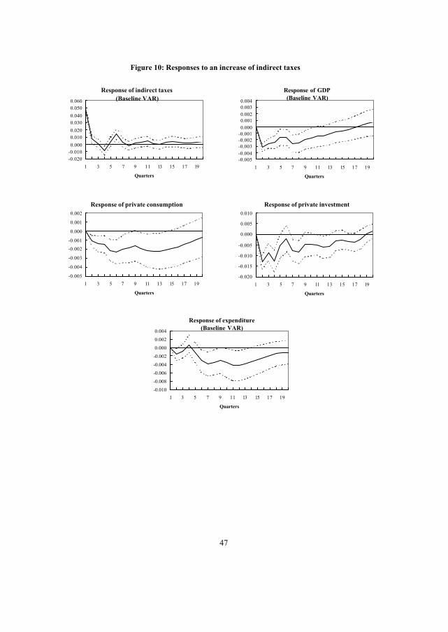
Figure 10: Responses to an increase of indirect taxes

Response of indirect taxes(Baseline VAR)

-0.020-0.0100.0000.0100.0200.0300.0400.0500.060

1 3 5 7 9 11 13 15 17 19

Quarters


-0.005

-0.004

-0.003

-0.002

-0.001

0.000

0.001

0.002

1 3 5 7 9 11 13 15 17 19

Quarters


-0.020

-0.015

-0.010

-0.005

0.000

0.005

0.010

1 3 5 7 9 11 13 15 17 19

Quarters


-0.005-0.004-0.003-0.002-0.0010.0000.0010.0020.0030.004

1 3 5 7 9 11 13 15 17 19

Quarters

Response of expenditure(Baseline VAR)

-0.010

-0.008

-0.006

-0.004

-0.002

0.000

0.002

0.004

1 3 5 7 9 11 13 15 17 19

Quarters

47

Figure 11: Responses to an increase of direct taxes

Response of direct taxes(Baseline VAR)

-0.020

-0.010

0.000

0.010

0.020

0.030

0.040

1 3 5 7 9 11 13 15 17 19

Quarters


-0.006-0.005-0.004-0.003-0.002-0.0010.0000.0010.0020.0030.004

1 3 5 7 9 11 13 15 17 19

Quarters


-0.025-0.020

-0.015-0.010-0.005

0.0000.005

0.0100.015

1 3 5 7 9 11 13 15 17 19

Quarters


-0.010

-0.008

-0.006

-0.004

-0.002

0.000

0.002

0.004

1 3 5 7 9 11 13 15 17 19

Quarters

Response of expenditure(Baseline VAR)

-0.005

0.000

0.005

0.010

0.015

1 3 5 7 9 11 13 15 17 19

Quarters

48

Figure 12a: Responses to an increase in government spending. Sample 1992Q1-2001Q2

Figure 12b: Responses to an increase in net taxes. Sample 1992Q1-2001Q2


-0.005-0.004-0.003-0.002-0.0010.0000.0010.0020.0030.004

1 3 5 7 9 11 13 15 17 19

Quarters

Response of GDP

-0.002

-0.002

-0.001

-0.001

0.000

0.001

0.001

0.002

1 3 5 7 9 11 13 15 17 19

Quarters


-0.020-0.015-0.010-0.0050.0000.0050.0100.0150.020

1 3 5 7 9 11 13 15 17 19

Quarters


-0.150

-0.100

-0.050

0.000

0.050

0.100

0.150

1 3 5 7 9 11 13 15 17 19

Quarters


-0.005

-0.004

-0.003

-0.002

-0.001

0.000

0.001

0.002

1 3 5 7 9 11 13 15 17 19

Quarters

Response of GDP

-0.002

-0.001

0.000

0.001

1 3 5 7 9 11 13 15 17 19

Quarters


-0.020

-0.010

0.000

0.010

0.020

0.030

0.040

1 3 5 7 9 11 13 15 17 19

Quarters


-0.150

-0.100

-0.050

0.000

0.050

0.100

0.150

1 3 5 7 9 11 13 15 17 19

Quarters

49

Documents

The macroeconomic effects of fiscal policy in Spain€¦ · DOCUMENTO DE TRABAJO Francisco de Castro BANCO DE ESPAÑA SERVICIO DE ESTUDIOS THE MACROECONOMIC EFFECTS OF FISCAL POLICY