The Modern Wholesaler:

Global Sourcing, Domestic Distribution, and Scale Economies

Sharat Ganapati, Yale University

sganapati.com, sganapati@gmail.com

⇤

Click here for the latest version

April 6, 2017

Abstract

Half of all transactions in the $6 trillion market for manufactured goods in the United Stateswere intermediated by wholesalers in 2012, up from 32 percent in 1992. Seventy percent of thisincrease is due to disproportionate growth by the largest one percent of wholesalers (i.e., theintensive margin). To understand the origins and implications of these findings, I develop amodel that incorporates downstream buyer demand with wholesaler market entry. Structuralestimates based on detailed administrative data from the U.S. Census Bureau reveal that therise of wholesalers was driven by an intuitive complementarity between their sourcing of goodsfrom abroad and an expansion of their domestic distribution network to reach more buyers. Bothelements require scale economies and lead to increased wholesaler market shares and markups.Counterfactual analysis shows that despite increases in wholesaler market power, intermedi-ated international trade has two benefits for buyers: first, through buyers’ valuation of globallysourced products, and second, through the passed-through benefits of wholesaler economies ofscale. The combined benefits of intermediated international trade in 2007 account for a $314billion net yearly increase in buyer surplus.

Keywords: international trade, intermediation, wholesale trade, geographic differentiation, im-ports, sourcing, returns to scale

⇤I am indebted to my advisors Pinelopi Goldberg and Costas Arkolakis and my dissertation committee membersSteve Berry and Peter Schott. I thank Joe Shapiro, Phil Haile, Samuel Kortum, and Lorenzo Caliendo for addi-tional valuable comments. This work was further guided by feedback from Andrew Bernard, Mitsuru Igami, DavidAtkin, Dan Ackerberg, Fiona Scott Morton, Giovanni Maggi, Kevin Williams, Meredith Startz, Jeff Weaver, MarceloSant’Anna, Jesse Burkhardt, Giovanni Compiani and Ana Reynoso as well as seminar participants at Yale, the 2015Federal Statistical Research Data Center Conference, and the 2016 WEAI and Econcon meetings. This work waspartially conducted with the support of the Carl Arvid Anderson Prize Fellowship. Jonathan Fisher and Shirley Liuat the New York Census Research Data Center and Stephanie Bailey at the Yale Federal Statistical Research DataCenter provided valuable data support. Peter Schott additionally provided concordance tables for international tradedata. Any opinions and conclusions expressed are those of the author and do not necessarily represent the views ofthe U.S. Census Bureau. All results have been reviewed to ensure that no confidential information is disclosed. Allerrors are mine.

1 Introduction

With advances in electronic communication technologies and falling trade costs, we imagine thatthe economy is moving to a frictionless state where buyers and sellers seamlessly connect, bypassingmiddlemen. However, in the distribution of manufactured goods, the opposite has occurred: usingrich United States administrative data over the last two decades, I show that middlemen are moreimportant than ever, doubling the value of distributed goods to three trillion dollars, expandingtheir distribution networks, and connecting domestic buyers to international markets. I find thatthese middlemen do not act as perfectly competitive firms that charge marginal cost. Rather, thelargest intermediaries compete in an increasingly oligopolistic manner, by combining internationaltrade with expanded domestic distribution networks to achieve greater scale economies.

This paper evaluates the implications of the expanding role played by wholesalers, a particulartype of middleman that sells almost exclusively to other businesses, in the distribution of goods in aglobalized economy. I make two principal contributions in this paper. First, I document the growingimportance of wholesalers in distributing imported and domestically produced manufactured goodswithin the United States and show that this increase is driven by the intensive margin, with thelargest wholesalers increasing in size. Second, I use a structural model to rationalize these trends,conduct counterfactuals to quantify their market consequences, and evaluate the role of wholesalersin globalization. In this model, wholesalers first enter, set up global sourcing and distributionnetworks, and determine prices. Downstream firms then decide to buy, choosing between using awholesaler or directly sourcing from a manufacturer.

Structural parameter estimates reveal that the largest wholesalers pay significant fixed coststo set up nation-wide networks to distribute globally sourced products. The increasing combinedfixed costs of international trade and expanded domestic distribution allow the largest wholesalersto exert more market power and raise prices. Downstream buyers receive two benefits from thesewholesalers: the immediate benefit of being able to source from abroad, and a secondary benefitwhere the largest wholesalers exploit increasing returns to scale and improve their distributionnetworks for domestically sourced products. Both benefits are underpinned by two interactingmechanisms. Wholesalers make investments, that are increasingly complementary, to (a) increasethe number of globally sourced varieties and (b) build better distribution networks within the UnitedStates. While I do not delve into the technology underpinning these investments in this paper, Iprovide preliminary evidence of the role of automation and software infrastructure.

This paper unfolds in four parts. First, it uses detailed micro data to characterize the natureand growth of the U.S. wholesale sector. In 2012, wholesale businesses in the United States sold$3.2 trillion in aggregate to downstream buyers. This large figure is driven by wholesaler growth,as transactions intermediated by wholesalers have grown faster than the overall market. From 1997to 2007, the share of transactions intermediated by wholesalers increased 34%, with internationallysourced varieties accounting for half of this gain. This growth is entirely driven by the intensivemargin, through increased market share of the largest 1% of wholesalers. This expansion corre-sponds to these large wholesalers increasing the number of imported varieties by 56% and domestic

2

distribution warehouses by 70%. In contrast, the median wholesaler rarely imported and saw nochange in the number of distribution centers. On the other side of the market, downstream buyersare shown to systematically prefer nearby wholesalers for smaller purchases, being ten times morelikely to to purchase through a wholesaler for shipments worth $1000 or less, compared to shipmentsworth over $1 million.

Second, this paper structurally estimates downstream buyer demand for wholesalers, allowingfor the decomposition of the gains from wholesaling. Downstream buyers can either indirectly sourceintermediate goods from a wholesaler at a markup over manufacturers’ prices an incurring a smallfixed cost, or they can pay a large fixed cost and directly source from a manufacturer, skipping thewholesaler markup and allowing for scale economies. My two-stage demand system captures thistradeoff. Geographically dispersed downstream buyers first choose how much to buy and then choosetheir optimal sourcing strategy from a set of wholesalers. Differentiated wholesalers compete hori-zontally (types of distributed varieties), vertically (distribution quality), and spatially (geographicreach).1 This discrete choice setup with heterogeneous buyers is estimated using both firm-leveland aggregated data to (a) accurately gauge price elasticities, (b) correct for price endogeneity, and(c) allow for multi-product wholesalers. The estimates from the demand model help explain whywholesalers have increased their market shares. The average wholesaler has made it even easier toindirectly procure intermediate goods, while only slightly increasing costs and markups. I find thatdownstream buyers’ value increases in wholesaler-distributed product varieties as well as expansionsin wholesaler domestic distribution networks. These gains more than offset increases in wholesalerprices due to the cost of international sourcing, rising market power, and an adverse shift in buyercomposition.2 In particular, downstream benefits increase the most for buyers from the largestwholesalers, who now provide substantially more international varieties and a denser network ofdistribution centers, without substantially increasing their prices.

Third, the model endogenizes the prices, attributes, and entry decision of wholesalers. In theabsence of detailed and accurate wholesaler cost data, I combine rich demand estimates with market-level assumptions to rationalize and estimate wholesaler costs. Using model-derived demand elastic-ities and first-order profit maximizing conditions, I recover wholesaler marginal costs and operatingprofits from a price-setting supply system with oligopolistic competitors. Subsequently, I considerthe entry costs of wholesalers, who make increasingly large fixed investments in (a) more efficientlysourcing products from far-flung foreign factories and (b) setting up domestic facilities to redistributethese products across the nation. Estimation, based on equilibrium conditions, finds that these twowholesaler innovations positively interact, with investment in international sourcing and domesticdistribution becoming increasingly complementary. This result, combined with demand estimates,

1Wholesalers exhibit a form of competition that is national in some respects, but local in others. For example,demand in the New York market is largely fulfilled by wholesalers in New York, but a large proportion comes fromneighboring New Jersey and Connecticut. Changes in prices, demand, and competition are all spatially interlinked.Estimation of supply and demand in such a market explicitly considers such inter-related regions.

2Are buyers changing or are wholesalers getting better? I find that buyers are growing systematically larger andbecoming more geographically clustered, which would indicate a decrease in wholesaling, as large buyers tend tosource directly from upstream manufacturers.

3

implies that wholesalers in 2007 provide much better products to downstream buyers compared towholesalers in 1997. However, to cover rising investment costs, these high-quality wholesalers requirelarge market shares to produce sufficient operating profits, driving up their market concentration.

Fourth, I quantify the gains from wholesaling by running counterfactuals under the fully esti-mated model. In the principal scenario, indirect sourcing via wholesalers for international products isrestricted to recover the downstream buyer gains from wholesaler-intermediated international trade.3

To disentangle the various benefits of wholesaling, I initially consider the static buyer gains (withoutwholesaler entry/exit) of indirect global sourcing through wholesalers. Subsequently, I recover thesecondary benefits that accrue though wholesaler scale economies by allowing wholesalers to makeentry and exit decisions based on expected profits. Through complementarities in investment, in-creases in international trade positively interact with the size of a wholesaler’s domestic distributionnetwork, compounding and nearly doubling the gain in aggregate buyer surplus. I show how themarket effects are mixed, with the largest wholesalers and smallest downstream purchasers comingout as winners. Specifically, the expansion of wholesalers into international trade in 2007 increaseddownstream purchase volumes by 5%, saving downstream buyers 8% in procurement costs as a per-centage of purchase value ($314 billion). However, due to the costs of investing in internationalsourcing, the largest 1% of wholesalers are able to increase their overall market share by 30% andtheir operating profits by 15%.

De Loecker and Van Biesebroeck (2016)4, summarizing recent work at the intersection of inter-national trade and industrial organization, find that trade studies largely ignore the distortionaryeffects of market power following the introduction or expansion of trade and simultaneously down-play the importance of intranational or localized competition between firms. This paper explicitlycorrects for these gaps in the current trade literature in the context of a very large and importantindustry. I find that trade-induced scale economies, as well as the importance of localized markets,lead to significant operating profits and reduced competition for wholesaler distributors. However,this downside is more than completely offset with the provision of massive reductions in relativeprocurement costs and gains from variety for downstream purchasers.

These results illustrate an important linkage between international trade and market concentra-tion. Public discourse (The Economist, 2016) has highlighted both increasing market power andmarket concentration across the economy as areas of general interest. Possible explanations for thislinkage include technological innovation, firm consolidation, and the influence of large, diversifiedshareholders. This paper introduces another mechanism: the increasing returns to scale introducedby the fixed costs of international trade and their interaction with domestic investments. Simulta-neously, these fixed costs can also explain the related phenomenon of the decreasing importance of

3Gains are all relative to sourcing directly from a manufacturer. Difficulty in sourcing from a manufacturer (bothdomestically and internationally) can offset gains from wholesaling. Future research will study this channel.

4They note that “...the interaction between efficiency and market power tends to be ignored. This is problematicas firms can use higher quality (imported) inputs or favorable locations to differentiate themselves and increase orgain market power” and “A final research avenue we believe to be promising is to study the distinction between localand global competition.”

4

smaller firms, who tend to be less efficient and exert less monopoly power.5

Related Literature

This paper is related to a number of important questions in empirical international trade, is basedon a set of theoretical microeconomic models, and is estimated using an industrial organizationestimation framework. I discuss these literatures in relation to this paper below:

International Trade In international trade, a variety of papers study wholesalers by leveragingtractable general equilibrium frameworks in the style of Melitz (2003). Such frameworks typically al-low for returns from scale due to international trade, but adopt a monopolistic competition structurethat generalizes away from variations in market power. These papers find various cross sectional pre-dictions that are verified in the data (Akerman, 2010; Ahn, Khandelwal and Wei, 2011; Felbermayrand Jung, 2011; Tang and Zhang, 2012; Crozet, Lalanne and Poncet, 2013). In general, these modelsfind that as fixed or variable trade costs fall, the share of trade passing through intermediaries willfall. Similarly, Rauch and Watson (2004), Petropoulou (2008), Antràs and Costinot (2011), andKrishna and Sheveleva (2014) consider alternative theoretical models for the gains from trade. Incontrast to this paper, these studies minimize market power and domestic trade considerations. Thispaper significantly contributes to the literature by allowing for wholesaler heterogeneity, downstreambuyer heterogeneity, and market power. Disregarding wholesaling, studies such as Pavcnik (2002),Gopinath, Gourinchas, Hsieh and Li (2011), Goldberg and Hellerstein (2013), and De Loecker, Gold-berg, Khandelwal and Pavcnik (Forthcoming) consider the effect of trade shocks and liberalizationon markups, firm productivity, and price pass-through. This principally reduced form literatureregresses firm outcomes on trade shocks; this paper directly considers a structural model to parseout the mechanism by which trade increases markups/productivity.6

Theoretical and Empirical Analysis of Intermediation There is an extensive theoretical lit-erature on intermediation.7 Early work by Rubinstein and Wolinsky (1987) endows intermediateswith a special matching ability to connect buyers and sellers.8 As summarized by Spulber (1999),these intermediaries can satisfy a variety of purposes: providing liquidity and facilitating transac-tions, guaranteeing quality and monitoring, market-making by setting prices, and matching buyerswith sellers. This paper empirically addresses these purposes, combining the costs of facilitating

5An alternate explanation may be that wholesalers allow smaller downstream firms to survive as they do not haveto run their own procurement networks.

6A burgeoning new literature exists in choosing the optimal source for intermediate inputs. Such work includesAntràs, Fort and Tintelnot (2014); Gopinath and Neiman (2014); Halpern, Koren and Szeidl (2015); Blaum, Lelargeand Peters (2015).

7A large operations management literature considers the best criteria for choosing an optimal source. Thesepapers tend to build on the economics of contracts literature (Tirole (1988) and Katz (1989)), but focus on theexplicit modeling of the operational details of production. See Tsay and Agrawal (2004) for an example.

8More detailed models as in Townsend (1983); Biglaiser (1993); Biglaiser and Friedman (1994) and Spulber(1996a,b, 1999) add various frictions to both buyers and sellers.

5

transactions and ensuring quality as fixed costs that must be paid by a wholesaler and which allowa wholesaler to charge markups.

The comprehensive structural empirical study of wholesaler markets is sparse. In internationaltrade, their presence has been also documented by Feenstra and Hanson (2004), Bernard, Jensen,Redding and Schott (2010), Bernard, Grazzi and Tomasi (2011), and Abel-Koch (2013), who all findthe rich and enduring presence of such intermediaries. Gopinath, Gourinchas, Hsieh and Li (2011)and Atkin and Donaldson (2012) study the role of prices and pass-through, but do not considerthe exact mechanisms that lead to pass-through.9 Bernard and Fort (2015) and Bernard, Smeetsand Warzynski (2016) explore the emergence of factory-less good producers, which account for aportion of the wholesale industry. As part of a larger NBER project exploring industrialization inthe United States, Barger (1955) summarizes the decline in the wholesale industry from 1869-1948.These papers all point to the importance of wholesalers, but consider their market structure as ablack box.

In industrial organization, recent papers by Salz (2015) and Gavazza (2011) consider informa-tional intermediaries and brokers, as opposed to physical good wholesalers.10 These papers addressSpulber’s last criteria, with wholesalers reducing the cost of matching buyers and sellers, and struc-turally estimate search models where informational brokers simplify the process of acquiring pricesor bids. Salz (2015) focuses on intermediaries both directly reducing search costs and providingan externality that reduces the prices paid by all buyers. In particular, such work abstracts awayfrom competition and quality differentiation between brokers and considers intermediary entry andmarkups as exogenous and invariant to market conditions. This paper endogenizes the entry ofmiddlemen and allows for endogenous middlemen markups. Papers such as Villas-Boas and Heller-stein (2006), Villas-Boas (2007), Nakamura and Zerom (2010), and Goldberg and Hellerstein (2013),consider retailers in a similar fashion to wholesalers. But these papers do not fully account for theincentives for such intermediaries outside of pricing.

Discrete Choice and Market Entry Methodologically this paper elaborates on the demand-side discrete choice framework of McFadden (1973).11 First, it builds on the logic of Hausman,Leonard and McFadden (1995) to allow for an endogenous market size. Second, the model uses awell-defined spatial component of demand as in Davis (2006). A set of aggregate moments fromsurvey data enables precise estimation of buyer heterogeneity as in Petrin (2002). Finally, whilemost demand estimates consider product attributes as exogenous, this paper endogenizes productattributes by combing a market entry model with reasonable timing assumptions along in vein of

9Gopinath et al. (2011) note that their findings suggest “that the correlation between the nominal and real exchangerate for the goods in our sample is not driven by local non-traded costs such as wages or by pricing to market atthe retail level, but rather by pricing to market at the wholesale level.” Atkin and Donaldson (2012) consider themarkups that occur between the factory gate or port of entry and final retail sale for a variety of consumer goods. Themarket structure of these intermediaries does not allow for heterogeneity; the authors assume a number of identicalmiddlemen under Cournot competition to derive welfare effects.

10In addition, these papers are closely related to papers that address real estate brokers. See Bar-Isaac and Gavazza(2015) for a recent example.

11A good overview of these techniques is found in Ackerberg et al. (2007).

6

Seim (2006), Eizenberg (2014), and Wollman (2014).This paper extends Hausman, Leonard and McFadden (1995), which uses Gorman (1970) to

adapt a two-stage demand system to a discrete-choice framework. Buyers decide how much to buybefore choosing the optimal source.12 While Hausman, Leonard and McFadden (1995) considers thenumber of vacations a consumer takes and fits a Poisson arrival function, this paper considers thenumber of downstream orders made and estimates a more general aggregate demand elasticity.13

In general, international trade papers consider an entire nation as a single market.14 However,is a relevant market a city, a state, or an entire nation? This paper’s model follows the spirit ofDavis (2006), Houde (2012) and Murry (2014) and allows for buyers to place differing valuations onsources by distance. While these papers allow for buyers to optimally choose among geographicallydispersed retailers, they still place exogenous restrictions on market size at the city or state levels;this paper extends such frameworks and allows for inter-regional shipments across the country.

The market entry setup takes into account sunk and fixed costs as in Sutton (1991) and Sutton(2001). Firms choose entry based on similar information structures to Seim (2006), where firmsenter based the expected value of operating profits and thus may face ex-post regret. The marketequilibrium solution concepts operate with firms satisfying plausible equilibrium assumptions assummarized in Berry and Reiss (2007).15

The remainder of the paper is as follows. Section 2 outlines the wholesaling industry, providesa case study, and presents a set of important descriptive facts. Section 3 describes the model. Sec-tion 4 explains identification and estimation. Sections 5, 6, and 7 summarize the estimation results,decompose results, and compute counterfactuals. Section 8 discusses alternative and complementaryexplanations and Section 9 concludes.

2 Data and Industry Facts

Market intermediaries come in many varieties and forms: some act as market-makers and others asdistributors. I focus on the latter, which are called wholesalers and defined by the US Census as:

... an intermediate step in the distribution of merchandise. Wholesalers are organizedto sell or arrange the purchase or sale of (a) goods for resale (i.e., goods sold to otherwholesalers or retailers), (b) capital or durable non-consumer goods, and (c) raw andintermediate materials and supplies used in production.16

12This approach contrasts with Hendel (1999), who combines the choice of how much to buy and whom to buy frominto a single stage and doesn’t consider the extensive margin of new buyers.

13A different type of two stage models are also frequently used in choice-set analysis. As reviewed by Manrai andAndrews (1998), buyers first choose a choice set and then choose the optimal choice from within this choice set.

14Arkolakis (2010) allows for a consumer-specific firm-level marketing cost, but still does not allow for firm-levelmarket power beyond monopolistic competition.

15While related work using moment inequalities allows for idiosyncratic fixed cost shocks, this method relaxes theparametric and distributional assumptions in estimating these shocks and allows for tractable counterfactual analysis.This extensive literature was developed econometrically and theoretically by Chernozhukov et al. (2007); Andrewsand Soares (2010); Andrews and Barwick (2012); Pakes et al. (2015). Select empirical examples include Ho and Pakes(2013); Eizenberg (2014); Wollman (2014).

16For full description see Appendix A.

7

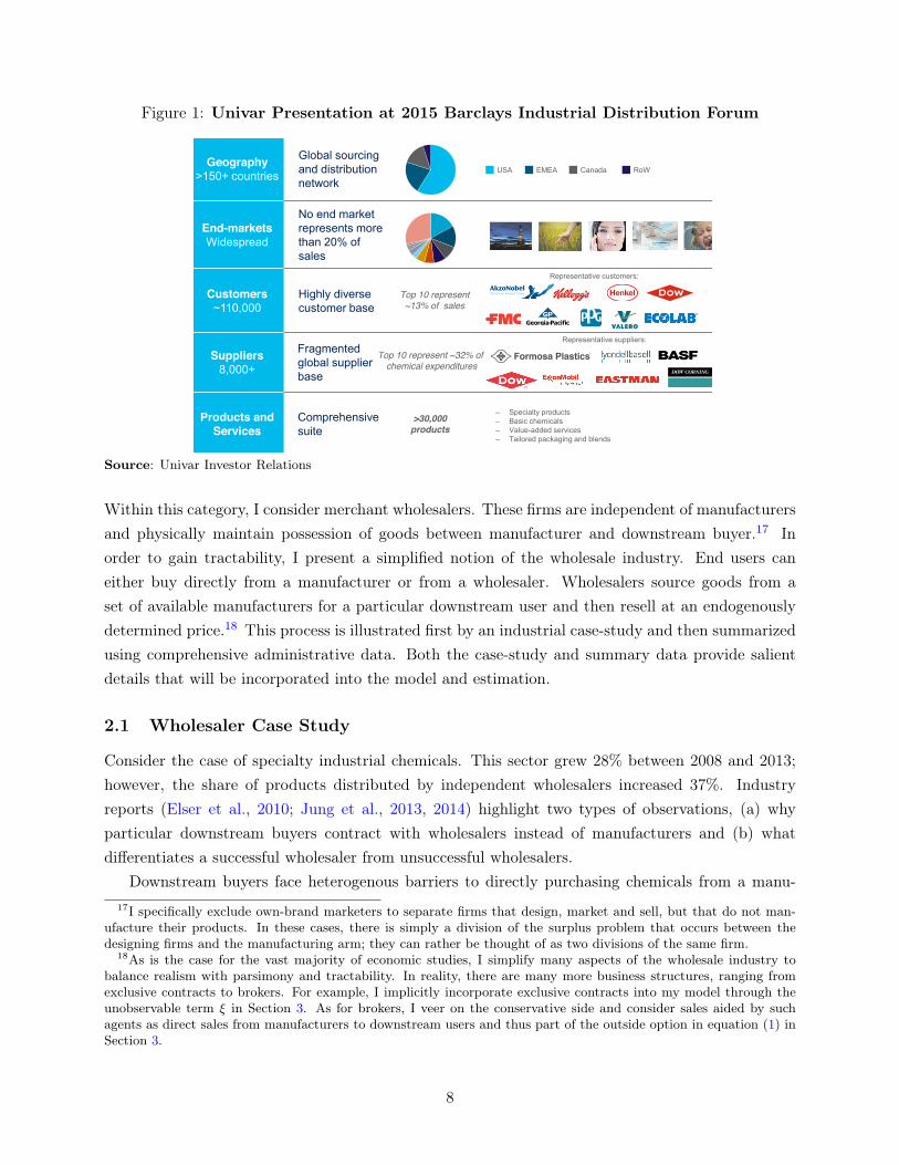
Figure 1: Univar Presentation at 2015 Barclays Industrial Distribution Forum

15 15

Business Diversity Provides Resilience and Stability

Geography >150+ countries

Global sourcing and distribution network

End-markets Widespread

No end market represents more than 20% of sales

Customers ~110,000

Highly diverse customer base

Suppliers 8,000+

Fragmented global supplier base

Products and Services

Comprehensive suite

>30,000 products

USA EMEA Canada RoW

– Specialty products – Basic chemicals – Value-added services – Tailored packaging and blends

Representative customers:

Top 10 represent ~13% of sales

Representative suppliers:

Top 10 represent ~32% of chemical expenditures

Well positioned for growth Source: Univar Investor Relations

Within this category, I consider merchant wholesalers. These firms are independent of manufacturersand physically maintain possession of goods between manufacturer and downstream buyer.17 Inorder to gain tractability, I present a simplified notion of the wholesale industry. End users caneither buy directly from a manufacturer or from a wholesaler. Wholesalers source goods from aset of available manufacturers for a particular downstream user and then resell at an endogenouslydetermined price.18 This process is illustrated first by an industrial case-study and then summarizedusing comprehensive administrative data. Both the case-study and summary data provide salientdetails that will be incorporated into the model and estimation.

2.1 Wholesaler Case Study

Consider the case of specialty industrial chemicals. This sector grew 28% between 2008 and 2013;however, the share of products distributed by independent wholesalers increased 37%. Industryreports (Elser et al., 2010; Jung et al., 2013, 2014) highlight two types of observations, (a) whyparticular downstream buyers contract with wholesalers instead of manufacturers and (b) whatdifferentiates a successful wholesaler from unsuccessful wholesalers.

Downstream buyers face heterogenous barriers to directly purchasing chemicals from a manu-17I specifically exclude own-brand marketers to separate firms that design, market and sell, but that do not man-

ufacture their products. In these cases, there is simply a division of the surplus problem that occurs between thedesigning firms and the manufacturing arm; they can rather be thought of as two divisions of the same firm.

18As is the case for the vast majority of economic studies, I simplify many aspects of the wholesale industry tobalance realism with parsimony and tractability. In reality, there are many more business structures, ranging fromexclusive contracts to brokers. For example, I implicitly incorporate exclusive contracts into my model through theunobservable term ⇠ in Section 3. As for brokers, I veer on the conservative side and consider sales aided by suchagents as direct sales from manufacturers to downstream users and thus part of the outside option in equation (1) inSection 3.

8

facturers. According to a 2009 Boston Consulting Group survey, 80% of downstream buyers withpurchases valued under €100,000 sourced goods indirectly through wholesalers, while larger pur-chasers nearly always sourced directly from a manufacturer. Downstream buyers value traditionaldistributor attributes such price, quality, and globally sourced varieties and are differentiated on twocharacteristics, their size and geographic location.19

In the industrial chemical market, wholesaler distributors perform three functions as they (a)source products from multiple manufacturers, (b) repackage these products, and (c) ship theseproducts to downstream buyers. While the global market for distributors is still fragmented, it isexperiencing rapid consolidation, with the three largest companies in 2011 holding 39% of the NorthAmerican market. In particular, the largest distributors have grown faster than the market, drivenby both organic expansion and market acquisitions. In contrast, smaller distributors face increasingfixed costs, as they try to “combine global reach with strong local presence.”

Consider one of the large speciality chemical distributors, Univar. Univar is a large industrialchemical wholesaler with North American shipments of approximately $10.4 billion in 2014. Thecompany was formed in 1928, increasing its distribution footprint through acquisitions and expan-sions. Today, it sources 30,000 varieties of chemicals and plastics from over 8,000 internationallydistributed suppliers. Univar uses its 8,000 employees to run a distribution network spanning hun-dreds of locations to supply 111,000 buyers. Univar’s business plan is summarized in a slide presentedas Figure 1.

Downstream buyers may need any of a variety of chemicals, and they may source these chemicalsdirectly from manufacturers such as DuPoint and BASF or indirectly through Univar. However,BASF and DuPont facilities may be located in distant locations and only stock their own productlines. Instead of individually sourcing chemicals, downstream buyers may pay a markup and haveUnivar do this for them, and have Univar source the shipments from each respective chemicalmanufacturer and reship them to a convenient loading bay. This tradeoff between convenience andprice is one of the central dynamics underpinning the wholesale industry. This also offers insightinto why the wholesale industry may be gaining market share, as the proliferation of new globalsources and varieties may make it harder to optimally source intermediate products for production.

2.2 Data Description

I bring together a variety of censuses and surveys conducted by the United States Census Bureau,Department of Transportation, and Department of Homeland Security covering international trade,domestic shipments and both the manufacturing and wholesale sectors. In particular, I use the Cen-sus of Wholesale Trade, Census of Manufacturers, Longitudinal Firm Trade Transaction Database,Commodity Flow Survey, and the Longitudinal Business Database, from 1992 to 2012.20

19Smaller downstream buyers “typically lack the critical mass needed to tap into low-cost sources for chemicals fromChina, Eastern Europe, or the Middle East.” In addition, these downstream buyers not only value price, productquality, and technical support, they prize flexibility and speed of delivery, which are highly correlated with geographicproximity.

20This draft only presents aggregated data for 2012. When available, micro-data will be used for 2012.

9

Table 1: Merchant Wholesaler Statistics

Year1997 2002 2007

Sales (2007 $’000) 6,544 7,854 9,995Merchandise Purchases for Resale (2007 $’000) 4,722 5,626 7,104International Sourcing (mean %) 17% 20% 23%Number of International Country Sources (mean) 0.565 0.69 0.793Number of International Country Source-Varieties (mean) 3.825 5.082 6.431Physical Locations (mean) 1.206 1.263 1.300Wholesaler Price (average Sales/Merchandise Purchases) 1.386 1.396 1.407

Product Markets 56 56 56Wholesalers 222,000 218,000 214,000

Average Number of Imported VarietiesSmallest 90% Wholesalers 1.2 1.6 2.2Middle 90-99% Wholesalers 13.7 18.0 24.6Largest 1% Wholesalers 137.4 183.6 213.8

Average Number of Domestic LocationsSmallest 90% Wholesalers 1.0 1.0 1.0Middle 90-99% Wholesalers 1.8 2.0 2.1Largest 1% Wholesalers 14.2 20.7 23.9

Notes: Varieties measured at the HS-8 level. Differences between cells in a row of means are all significant withp < .01.

These databases are linked together every 5-years at the firm level and provide at the aggregatelevel the share of goods distributed by a wholesaler in 56 distinct product categories, correspondingto North American Industry Classification System (NAICS) 5-digit sectors. I will treat each of theseproduct categories as an independent market. I focus on wholesalers independent of manufacturingestablishments and collect details on each wholesaler’s aggregate sales, physical locations, operatingexpenses, and the extent of international trade.21 Additionally survey data provides statistics on thedistribution of the origin, destination, and size of shipments across wholesalers and manufacturers.One limitation of the shipment data is the lack of information on the identity of downstream buyers;I only know the quantity purchased and their geographic location. This will have serious implica-tions on my modeling choices. Certain industries related to petroleum, alcohol, and tobacco areremoved due to data issues. Further details and the process of merging these databases is detailedin Appendix A.

This analysis is based on quantities in terms of producer prices. There are multiple reasons fordoing this, and the first is due to the availability of data. While certain small industries producequantity data, they form only a small portion of the overall goods economy. Secondly, when available,

21These operating expenses are not equivalent to marginal costs, as they are derived from balance sheet data andmay or may not include rents on capital and other fixed investments.

10

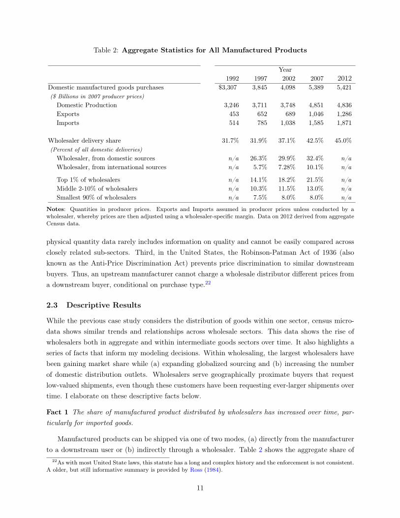
Table 2: Aggregate Statistics for All Manufactured Products

Year1992 1997 2002 2007 2012

Domestic manufactured goods purchases($ Billions in 2007 producer prices)

$3,307 3,845 4,098 5,389 5,421

Domestic Production 3,246 3,711 3,748 4,851 4,836Exports 453 652 689 1,046 1,286Imports 514 785 1,038 1,585 1,871

Wholesaler delivery share(Percent of all domestic deliveries)

31.7% 31.9% 37.1% 42.5% 45.0%

Wholesaler, from domestic sources n/a 26.3% 29.9% 32.4% n/aWholesaler, from international sources n/a 5.7% 7.28% 10.1% n/a

Top 1% of wholesalers n/a 14.1% 18.2% 21.5% n/aMiddle 2-10% of wholesalers n/a 10.3% 11.5% 13.0% n/aSmallest 90% of wholesalers n/a 7.5% 8.0% 8.0% n/a

Notes: Quantities in producer prices. Exports and Imports assumed in producer prices unless conducted by awholesaler, whereby prices are then adjusted using a wholesaler-specific margin. Data on 2012 derived from aggregateCensus data.

physical quantity data rarely includes information on quality and cannot be easily compared acrossclosely related sub-sectors. Third, in the United States, the Robinson-Patman Act of 1936 (alsoknown as the Anti-Price Discrimination Act) prevents price discrimination to similar downstreambuyers. Thus, an upstream manufacturer cannot charge a wholesale distributor different prices froma downstream buyer, conditional on purchase type.22

2.3 Descriptive Results

While the previous case study considers the distribution of goods within one sector, census micro-data shows similar trends and relationships across wholesale sectors. This data shows the rise ofwholesalers both in aggregate and within intermediate goods sectors over time. It also highlights aseries of facts that inform my modeling decisions. Within wholesaling, the largest wholesalers havebeen gaining market share while (a) expanding globalized sourcing and (b) increasing the numberof domestic distribution outlets. Wholesalers serve geographically proximate buyers that requestlow-valued shipments, even though these customers have been requesting ever-larger shipments overtime. I elaborate on these descriptive facts below.

Fact 1 The share of manufactured product distributed by wholesalers has increased over time, par-

ticularly for imported goods.

Manufactured products can be shipped via one of two modes, (a) directly from the manufacturerto a downstream user or (b) indirectly through a wholesaler. Table 2 shows the aggregate share of

22As with most United State laws, this statute has a long and complex history and the enforcement is not consistent.A older, but still informative summary is provided by Ross (1984).

11

domestic absorption of manufactured goods distributed by all wholesalers from 1992 to 2007. In1992, wholesalers accounted for the distribution of just 32% of all manufactured goods. In contrast,in 2007, wholesalers accounted for 42.5% of all shipments to downstream buyers.

Such aggregate trends may be caused by compositional shifts across product types. In particular,products such as chemicals with large wholesale shares have increased in importance over time. Aregression with appropriate controls accounts for this possibility. I regress the wholesaler marketshare by product type23 with yearly and product type fixed effects for 1997, 2002 and 2007 acrossapproximately 400 product types.

wholesale sharei,t = .33

(.01)+ .05

(.01)⇥ I2002 + .09

(.02)⇥ I2007 + ~

�Ii + ✏it

r

2= .92

observations ⇡ 1200

Regressors It are dummy indicators by years, and Ii are indicators for product types. Theseresults imply that wholesale shares increased on average by 5 percentage points from 1997 to 2002and another 4 percentage points from 2002 to 2007, broadly reflecting the change in aggregate marketshares.

Simultaneously, the proportion of goods distributed by wholesalers and acquired abroad hassimilarly increased. The trend is highlighted in Table 2. In 1997, such products accounted for 18%of wholesaler sales and 6% of all domestic purchases. By 2007, these products made up 32% ofwholesalers sales and 10.1% of all domestic purchases.

Fact 2 Wholesalers are becoming more heterogeneous, with the largest wholesalers increasing market

shares and importing a larger share of their products.

Most work on intermediates treat wholesalers in this sector as identical within a market. Asshown in Tables 1 and 2, there is incredible heterogeneity in wholesalers, both inter-temporallyand cross-sectionally.24 Over just 10 years, the average wholesaler has nearly doubled real salesand become 35% more likely to source products internationally, from where they import 68% morevarieties at the Harmonized System 8-digit category level. On average, these wholesalers increasedthe number of domestic distribution centers by 8%, all while decreasing average prices.

Changes across time provide insight into why certain wholesalers are increasing their marketshares. The average wholesaler in the 99.5th percentile of a sector by sales controls nearly 1% ofthe national market, a share hundreds of times larger than the smallest wholesaler. Consideringgeographic and quantity market segmentation, this can easily translate to large effective marketshares in particular segments and thus the ability to exert market power. Additionally, these largewholesalers are differentiated in many other ways; compared to a median wholesaler, they are 4

23I used the SCTG 5-digit code from the Commodity Flow Survey. Similar results hold at higher levels of aggrega-tion.

24Detailed statistics are available in Appendix Tables A1 - A4

12

Table 3: Geographic Spread

2002 Share of Domestic ShipmentsSource/Destination Wholesalers Manufacturers

Same State 54% 32%Same Census Region 67% 47%Same Census Division 75% 60%

Notes: Each cell represents the percent of shipment by overall type of shipper within a geographic scope.

times more likely to import goods from abroad and have nearly 20 times more domestic distributioncenters.

Even starker are the inter-temporal trends across wholesalers The 99th percentile of wholesalershave increased their aggregate market shares 50%, while increasing the average number of importedproduct varieties from 140 to 210 and the number of distribution locations by 68%. In contrast,the median wholesaler’s market share stayed constant, with no measurable change in the numberof domestic distribution centers. Substantial heterogeneity may imply that larger wholesalers makestrategic competitive decisions, while the smallest wholesalers are too small to exert market power.

Having focused primarily on the upstream aspect of the data, I shift to describing the natureand types of buyers in my model.

Fact 3 Wholesalers, in contrast with manufacturers, predominantly ship products to nearby desti-

nations.

Wholesalers specialize in local availability: they form a middle link in getting goods from afactory to retailers and downstream producers. This fact is illustrated in Table 3. For example, awholesaler is nearly 70% more likely than a manufacturer to conduct a shipment within the samestate. The preponderance of local shipments allows wholesalers with distribution centers in relativelyisolated locations to exert local market power.

Fact 4 Smaller buyers predominantly deal with wholesalers, instead of manufacturers.

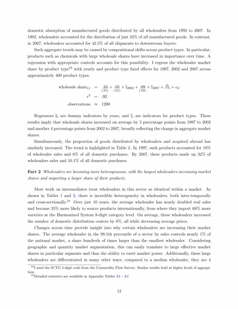
Downstream wholesaler shipments are of much smaller value than manufacturer shipments. Ta-ble 4 shows that shipments worth $1000 or less in producer prices account for 15% of total wholesalershipments, but only 4% of manufacturer shipments. In contrast, shipments of over $1,000,000 ac-count for only 3% of wholesaler shipments, but 15% of manufacturer shipments. Certain wholesalersmay exert market power in small shipments, even if they exhibit smaller overall market shares.

Fact 5 The distribution of buyer types has skewed towards larger shipments over time.

One hypothesis explaining the shift towards wholesaling is the spread of “just in time” man-ufacturing and supply practices. These business models forgo a small number of large deliveriesfor a larger number of smaller shipments. This provides downstream buyers with more flexibility

13

Table 4: Shipment Size in Producer Prices

Shipment Size % by Shipper Type % by Shipment Typelog ($) $

0000 Wholesalers Manufacturers Wholesalers Manufacturers

<6 <1 14.9% 3.9% 71.4% 28.6%7-8 1- 3 12.9% 4.7% 64.1% 35.9%8-9 3- 8 16.9% 8.7% 55.9% 44.1%9-10 8 - 22 24.0% 16.1% 49.3% 50.7%10-11 22 - 60 14.4% 22.8% 29.0% 71.0%11-12 60 - 160 8.8% 19.1% 22.9% 77.1%12-13 160 - 440 4.7% 9.4% 24.3% 75.7%13-14 440 - 1,200 2.1% 5.8% 19.2% 80.8%>14 >1,200 1.3% 9.5% 7.9% 92.1%

Notes: Figures in real 2007 dollars. Quantities equal revenues in producer prices. First two columns each sum to 1.Each row in the last two columns sum to 1.

Figure 2: Distribution of Buyers

0%

5%

10%

15%

20%

25%

<$1000 >$1.2M

Shareo

fPurchases

BuyerPurchaseSizePerShipment(InProducer$)

1997 2002 2007

Figures in real 2007 dollars.

14

Figure 3: Model Timing

Wholesaler Pricing: t2Market Size: t3

Individual Buyer Choice: t4IID Downstream Shock

Aggregate Shocks

Quality + Cost ShocksWholesaler Entry: t1

and reduces inventory costs. In aggregate, such practices would imply that there is a shift towardssmaller order sizes. If wholesalers are more adept at shipping smaller orders, then this may inducea shift of buyers switching to wholesalers. However, this has not occurred, as shown in Figure 2.Downstream buyers have slightly increased the average size of their orders over time.25

3 Model

To compute downstream gains from wholesaling, I construct a demand system paired with a whole-saler supply and entry model. Estimates from the demand model can determine downstream valua-tions for prices and various wholesaler attributes such as international sourcing. The supply modelconsiders the relationship of prices with underlying marginal costs and market competition. Thesetwo stages will help determine the underlying forces driving the increase in wholesaler market shares.Finally, the wholesaler market entry game will produce entry cost estimates for counterfactual esti-mation.

3.1 Model Overview

There are four periods, t1 � t4. Periods t1 � t2 consider the decisions made by wholesalers. Att1, wholesalers make market entry decisions and at t2 wholesalers choose their prices. I will referto stages t1 and t2 as wholesaler entry and wholesaler pricing respectively. Periods t3 and t4

involve the decisions made by downstream buyers searching for suppliers. At period t3, aggregatedownstream demand is determined, and downstream buyers choose how much to buy. Finally at t4,downstream buyers choose between indirectly sourcing through wholesalers or directly sourcing fromupstream sources. I will call stages t3 and t4 market size and downstream choice respectively.

In a pre-period t0, the characteristics of upstream producers and manufacturers are made, theydetermine what to produce and how much to charge for it. This empirical strategy will take decisionsmade at t0 as exogenous and open for future analysis; the focus will be on estimating and solvingstages t1 through t4.

To aid in identification, wholesalers’ entry and investment choices are consolidated in t1. Whole-salers first decide to enter a market and choose their market position. In practice this means that

25A related fact shows that the geographic distribution of buyers has not significantly changed over the same timeperiod.

15

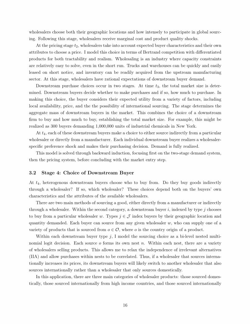
wholesalers choose both their geographic locations and how intensely to participate in global sourc-ing. Following this stage, wholesalers receive marginal cost and product quality shocks.

At the pricing stage t2, wholesalers take into account expected buyer characteristics and their ownattributes to choose a price. I model this choice in terms of Bertrand competition with differentiatedproducts for both tractability and realism. Wholesaling is an industry where capacity constraintsare relatively easy to solve, even in the short run. Trucks and warehouses can be quickly and easilyleased on short notice, and inventory can be readily acquired from the upstream manufacturingsector. At this stage, wholesalers have rational expectations of downstream buyer demand.

Downstream purchase choices occur in two stages. At time t3, the total market size is deter-mined. Downstream buyers decide whether to make purchases and if so, how much to purchase. Inmaking this choice, the buyer considers their expected utility from a variety of factors, includinglocal availability, price, and the the possibility of international sourcing. The stage determines theaggregate mass of downstream buyers in the market. This combines the choice of a downstreamfirm to buy and how much to buy, establishing the total market size. For example, this might berealized as 300 buyers demanding 1,000,000 units of industrial chemicals in New York.

At t4, each of these downstream buyers make a choice to either source indirectly from a particularwholesaler or directly from a manufacturer. Each individual downstream buyer realizes a wholesaler-specific preference shock and makes their purchasing decision. Demand is fully realized.

This model is solved through backward induction, focusing first on the two-stage demand system,then the pricing system, before concluding with the market entry step.

3.2 Stage 4: Choice of Downstream Buyer

At t4, heterogenous downstream buyers choose who to buy from. Do they buy goods indirectlythrough a wholesaler? If so, which wholesaler? These choices depend both on the buyers’ owncharacteristics and the attributes of the available wholesalers.

There are two main methods of sourcing a good, either directly from a manufacturer or indirectlythrough a wholesaler. Within the second category, a downstream buyer i, indexed by type j choosesto buy from a particular wholesaler w. Types j 2 J index buyers by their geographic location andquantity demanded. Each buyer can source from any given wholesaler w, who can supply one of avariety of products that is sourced from o 2 O, where o is the country origin of a product.

Within each downstream buyer type j, I model the sourcing choice as a bi-level nested multi-nomial logit decision. Each source o forms its own nest n. Within each nest, there are a varietyof wholesalers selling products. This allows me to relax the independence of irrelevant alternatives(IIA) and allow purchases within nests to be correlated. Thus, if a wholesaler that sources interna-tionally increases its prices, its downstream buyers will likely switch to another wholesaler that alsosources internationally rather than a wholesaler that only sources domestically.

In this application, there are three main categories of wholesaler products: those sourced domes-tically, those sourced internationally from high income countries, and those sourced internationally

16

from low income countries.26 A wholesaler who procures products from multiple sources (say bothdomestic and foreign products) is considered a multi-product firm that sells products in multiplenests. I place products sold by multi-product wholesalers in their own respective nests. This impliesthat purchases from these multi-source wholesalers could be more substitutable with other multi-source wholesalers than with single-source wholesalers. For manufacturers, who are not the mainfocus of this paper, all possible sources are collected together and valued as the outside option (some-times denoted as direct sourcing). I run this analysis for many product markets m, but suppressthis subscript for clarity. See Figure 4 for a simplified example with just one foreign source.27

A customer i of type j buys from the from wholesaler w in nest n that provides the highestindirect utility:

Ui,j,w,n = �j,w,n + ✏i,j,w,n. (1)

Wholesalers w provide mean benefit �j,w,n to all buyers of type j when selling products from aproduct nest n and customer-specific deviation ✏i,j,w,n. This ✏ is unobserved by the econometricianand can represent unmeasured variables, optimization errors, and idiosyncratic preferences.

Following McFadden (1980) and Cardell (1997), I break up the unobserved deviation ✏ into threeadditive terms:

✏i,j,w,n = ⌫

oi,j,n (�o) + ⌫

ni,j,n (�o,�n) + (1� �o) (1� �n) ✏i,j,w,n

The two ⌫ (·) terms incorporate the unobserved idiosyncratic taste of buyer i to wholesalers toproducts in nest n, and the residual disturbance ✏i,j,w,n is assumed to be drawn from a standardGumbel distribution. The parameter � = (�o,�n) captures the relative weighting between ⌫ and✏.28 The first ⌫o denotes the correlation of ✏ between direct sourcing, indirectly sourcing from high-income foreign countries, and indirectly sourcing from low-income foreign countries. This allows forproducts sourced from abroad to be imperfect substitutes for domestically sourced products. Thesecond ⌫

n denotes the correlation of ✏ of multi-source and single-source wholesalers conditional onsourcing from the same location. This allows for domestic products sourced by globalized wholesalersto be imperfect substitutes for products sourced by domestic-only wholesalers. The parameter �captures the extent to which a buyer prefers a product in a particular nest. In this model, a large�n near 1 implies that products within a given nest are more highly substitutable within the nestthan outside it. I consider alternative forms for ✏ in the Appendix.29

26This is a generalization of the Armington assumption that there is imperfect substitution between foreign anddomestic varieties.

27In this main specification there are 7 disjoint nests; (1) directly sourced products from manufacturers, (2) productssourced domestically by single-source wholesalers, (3) products sourced from low-income countries by single-sourcewholesalers, (4) products sourced from high-income countries by single-source wholesalers, (5) products sourced do-mestically by multi-source wholesales, (6) products sourced from low-income countries by multi-source wholesalers,and (7) products sourced from high-income countries by multi-source wholesalers.

28The distribution ⌫ is uniquely defined in Cardell (1997). Additionally �type > �source and both � 2 [0, 1).29In the Appendix, I allow for one levels of nesting, with the product source (direct, indirect domestic, indirect high

income foreign, and indirect low-income foreign) interacted by wholesaler type (grouping single-source wholesalers

17

Figure 4: Stage 4 - Simplified Sourcing Error Variance Tree Diagram

Unobserved Downstream Buyer Sourcing Correlations

Direct SourcingFrom Manufacturer

Nests

WholesalerDomestic Product

Diversified Wholesalers

w3,d w4,d

Domestic-only Wholesalers

w1,d w2,d

WholesalerForeign Product

(High Income Source)

Diversified Wholesalers

w3,fh w4,fh

Foreign-only Wholesalers

w5,fh w6,fh

WholesalerForeign Product

(Low Income Source)

Diversified Wholesalers

w3,fl w4,fl

Foreign-only Wholesalers

w7,fl w8,d

WholesalerTypes (σn)

SourceTypes (σo)

Outside option

Notes: This tree diagram lists the correlation patterns for unobserved buyer valuations ✏. The top level differentiatesforeign and domestic sources. The second level differentiates wholesalers that sell both foreign and domesticallysourced products from those that only sell either foreign or domestically sourced products. The bottom level nestsdifferentiates between wholesalers, the first subscript denotes the identity of the wholesaler and the second subscriptdenotes the sourcing of a product. The model allows for two different types of foreign sources, those from high-incomecountries and from low-income countries. Wholesalers can belong to multiple bottom level nests, colors highlightwholesalers that participate in multiple nests. Additionally, all direct sourcing in lumped together in an outsideoption. Alternative nesting patterns are listed in the Appendix.

The mean valuation (�j,w,n) of wholesaler w selling product in nest n for buyer of type j, can bedecomposed into observed and unobserved components:

�j,w,n = fj (pw,n, lw,n,aw,m, qj , lj) + ⇠w,n (2)

The function fj (·) captures the preference of buyer type j for a particular wholesaler w sellingproducts in nest n. These preferences are a function of both wholesaler and buyer attributes.In particular, the wholesaler price (pw,n), wholesaler location (lw,n) and observable characteristics(aw,n). The vector aw,n includes characteristics of the wholesaler, such as the number and varietyof international sources, as well as market-level observables, which include market-year fixed effectsas well as indicators for the source of the good and the location of the wholesaler. There are tworelevant buyer attributes: their location (lj ) and their purchase size (qj). Purchase size qj is binnedinto nine groups for tractability. The residual ⇠w,n denotes the unobserved quality of wholesaler w

selling products in nest n; it is realized between stages t3 and t4.I use a linear functional form for �:

�j,w,n = ↵

plog pw,n + ↵

l�stateIl�statew,n,j + ↵

l�regionIl�regionw,n,j + ↵

qlog qj + aw,n↵

a+ ⇠w,n (3)

separately from multiple-source wholesalers). Results are largely unchanged. Robustness tests available on requesttest and reject alternative nesting structures. Non-nested models and generalized mixed logit models, in the vein ofBresnahan et al. (1997) find similar results.

18

The indicator function Ilw,n,j captures the interaction of lj and lw,n; Il�statew,n,j equals one when the

wholesaler and buyer are in the same state and Il�regionw,n,j equals one when the wholesaler and buyer

are in the same Census region. The vector ↵ =

�↵

p,↵

l,↵

q,↵

a�

captures buyer’s sensitivity towholesaler prices, location choices, purchase quantities, and observable characteristics. In particularthe parameters ↵p and ↵

q allow me to capture the trade-off between the variable cost of buying q

units at price p from a wholesaler with the fixed cost of directly sourcing q units of the good from themanufacturer. For a micro-foundation of this particular setup in relation to a downstream buyer’scost minimization problem, see Appendix B.

Conditional wholesaler market share Within buyer type j, the model follows a nested logitspecification (McFadden, 1980) and aggregates across downstream buyers values for their buyer-specific shock ✏. The probability of a purchase from wholesaler w, conditional on a downstreampurchaser type j is a function of mean valuation �j,w,n and parameters �:

sw,n|j = s (�j,w,n;�) . (4)

This function s (·) has a closed form and is derived in Appendix (B.5).

Wholesaler market share The overall market shares of a wholesaler w in nest n aggregatesacross a wholesaler’s market share across all j types of buyers:

sw,n =

X

j2Jsw,n|jµjdj (5)

Where sw,n|j represents the market share of wholesaler w with buyers of type j and µj denotesthe relative mass of buyers of type j. Observed and recovered wholesaler and product attributesare collected as x = [p a ⇠]. While the mass of buyers µj is exogenous in this step, the next stependogenizes this choice.

3.3 Stage 3: Market Size

At t3, downstream buyers make two decisions. First, buyers decide if they should make a purchase.Second, buyers decide how much to buy. Aggregated, these two steps establish the total downstreammarket size by considering both the mass of buyers and their purchase quantities.

Generally, discrete choice models assume that the total mass of possible buyers and their purchasequantities (conditional on buying) are fixed. However, this assumption is not plausible across allintermediate manufactured good markets. If a set of wholesalers enter, perhaps supplying goodsfrom a new foreign market, there may be an increase in the overall downstream market size.

I combine both the number of buyers and how much they buy in a single step. In particular,I consider the elasticity of a market size for a buyer of type j with respect to the valuation of allwholesaler options. While adopting a slightly different functional form, this stage follows Hausmanet al. (1995), where buyers first choose quantity before choosing among a set of discrete choices. This

19

quantity choice incorporates information from the choice set in a parsimonious manner and modelsa situation where buyers must pick their purchase quantities before receiving their idiosyncratic costdraws ✏.

In the absence of aggregate company size data for downstream buyers, I directly consider eachdownstream purchase as an independent purchaser.30 The number of purchasers of type j varieswith the vector x of wholesaler attributes. This allows for an increase in the number of purchasesfollowing increases in aggregate wholesale supplier quality. First, I denote the market share ofpurchases from buyer type j as:

µj =

qjMj (x)P&2J q&M& (x)

.

The set J collects all possible types j. Let Mj (x) denote the mass of downstream buyers of typej and qj their purchase quantities. This function Mj (x) captures two margins; downstream buyerscan (a) choose to make a purchase or (b) change the quantity purchased due to changes in marketcharacteristics x. I assume the number of downstream buyers Mj is a function of their expectedutility, which is denoted as:

Mj (x) = m (EUj)

where m (·) denotes some monotone increasing function, and EUj = Ej [maxw,n Ui,j,w,n] denotes theexpected utility for a buyer of type j integrating across ✏. This expected utility is determined relativeto the utility of directly sourcing from an upstream producer (outside option) and is determined upto a constant.

I parameterize this downstream buyer mass Mj as:

Mj (x) = Aj ⇥ (EUj)�. (6)

The parameter � denotes the elasticity of the number of purchasers relative to the aggregate valuationof purchases. The shifter Aj represents demand by downstream buyers of type j in the absence ofwholesalers. In particular, as shown in Appendix B, this form of two stage decision making isconsistent with simple forms of cost minimization, when costs are realized after production choices.This discrete choice setup allows me to directly measure relative expected utility EUj using the

overall wholesaler share, as EUj =

⇣1� S

Wj

⌘�1. The variable S

Wj is the summed market share of

all wholesalers selling to buyer type j:

S

Wj =

X

w2W

X

n2Nw

sw,n|j .

The set W refers to all wholesalers, and the set Nw refers to the nests wholesaler w sells in.30An alternative formulation would consider the total purchase quantities, however this would require considering

downstream buyers as ex-ante identical, before they make their purchase quantity decisions.

20

Taking logs, I obtain the relationship:

logMj = �� log ⇥1� S

Wj

⇤+ logAj . (7)

This relationship assumes that downstream buyers only realize shocks ✏ in equation (1) once theystate their intent to buy a certain number of goods. For example, suppose a downstream manu-facturer is considering the use of a new chemical in their production process. If the manufacturerperceives these chemicals to be cheap, they will choose to make a purchase; otherwise, they will not.This decision will rely only on the expectation of the shocks ✏, along with the set of purchase optionsand their attributes, which are summarized by EUj and Aj .

Parameters from both demand stages are collected as ✓ = [↵ � � A]. With the downstreambuyer choice problem fully described, the model now describes the behavior of wholesalers.

3.4 Stage 2: Wholesaler Pricing and Marginal Costs

In stage t2, I assume wholesalers compete on price, selling differentiated products.31 This allows meto use a wholesaler’s profit maximization conditions to recover and decompose their marginal costs,and to measure operating profits.

Wholesalers first post their prices and then sell any quantity demanded at that price. As whole-salers are not directly involved in production, they can find sources to meet any reasonable demandedquantity in the short run (see Spulber (1999) for examples).

Wholesaler w maximizes their total operating profits:

⇡w =

X

n2Nw

(pw,n � cw,n)Qw,n (p, ¯x; ✓) , (8)

where pw,n and cw,n represent the price and marginal cost of wholesaler w’s products in nest n 2 Nw.Nw denotes the set of nests/sources for wholesaler w. For example, a multi-source wholesaler mustchoose a price for their domestically sourced and internationally sourced products. The functionQw,n (·) denotes the expected number of purchases conditional of all other wholesalers’ prices p aswell as their non-price attributes ¯

x = [x/p] and takes the form:

Qw,n (p, ¯x; ✓) =

X

j2Jsw,n|j (p, ¯x; ✓) qjMj (p, ¯x; ✓) .

The conditional share function sw,n|j (·) is defined in equation (4) and the market size function Mj (·)is defined in equation (6) for different purchasers buying quantity qj .

Taking the derivative of operating profits with respect to prices and assuming profit maximiza-31I assume pure-strategy prices, that are assumed to be uniquely determined. This is a typical assumption in the

differentiated product demand literature, as in Nevo (2001); Eizenberg (2014). This assumption can by rationalizedwith the conditions imposed in Caplin and Nalebuff (1991).

21

tion, I can derive the marginal cost cw,n as a function of market observables and demand:

c

⇤w,n = c

✓pw,n, Qw,n,

dQw,n0

dpw,n;n, n

0 2 Nw

◆. (9)

This is a function of not only wholesaler price (pw,n) and quantity sold (Qw,n), but also the salesresponsiveness of wholesaler w’s product in nest n (say internationally sourced) with respect to theprice (dQw,n/dpw,n) and the sales responsiveness to the price for some other product in a differentnest n0 (say domestically sourced) sold by the same wholesaler

�dQw,n0

/dpw,n

�. See Appendix C for

a full derivation.These wholesalers face constant marginal costs c⇤w,t, which are a function of observable, recovered,

and unobserved wholesaler-source attributes:32

c

⇤w,n = c (

˜

xw,n, ⌫w,n) = ˜

xw,n� + ⌫w,n. (10)

The vector ˜x = [x/p] includes wholesaler observables, such as the extent of international sourcingand number of domestic distribution locations, as well as the recovered wholesaler-source specificquality shock ⇠ from the demand choice stage. The model also allows for a univariate unobservedmarginal cost shifter ⌫.

3.5 Stage 1: Wholesaler Market Entry

In stage t1, wholesalers make entry decisions and pay fixed cost to realize their attributes x, qualityshocks ⇠, and marginal cost shocks ⌫. When entering the market, wholesalers make two simultaneouschoices: their importing profile and the configuration of their domestic distribution network.

In implementation, N wholesalers are observed entering as with configuration a, which is com-posed of the sourcing strategy s ⇢ S and location configuration l ⇢ L. Sourcing strategies can takeone of several main forms: wholesalers can choose to source domestically, from high-income foreignsources, and/or source low-income foreign sources. Furthermore, wholesalers can choose the numberof foreign varieties to source. Combined, these possibilities form the set S. In terms of distribution,wholesalers can choose to set up distribution in any of the fifty states along with the District ofColumbia.

As in most entry models, this model does not necessarily have a unique equilibrium. It is possiblethat one equilibrium allows for only small wholesalers and another equilibrium allows for only largewholesalers. However, fixed entry costs may still be identified in these models, under the assumptionthat the current market configuration is some equilibrium.33 In particular, two conditions must hold:(1) wholesalers will only enter if their expected operating profits are greater than entry costs, and(2) additional wholesalers of a type will not not earn expected operating profits greater than entrycosts. Once wholesalers pay these fixed costs Ea and enter the market, each wholesaler receives a

32Constant marginal cost does not imply constant returns to scale, as wholesalers pay upfront fixed costs to realizeattributes x in the first stage.

33For an example, see Berry et al. (2015).

22

draw ⇠ that shifts a buyer’s valuation, and ⌫ that shifts marginal costs for the products sold.Returning to the equilibrium conditions, (1) implies that the the upper bound of entry cost ¯

Ea

is:Ea EN

⇠,⌫ [⇡ (a) |N ] =

¯

Ea (11)

The notation EN⇠,⌫ [·|N ] denotes the expectation over random variables (⇠, ⌫) conditional on N whole-

salers of type a = (s, l) participating.If the current market configuration is an equilibrium, then it would be unprofitable for an addi-

tional wholesaler to enter with sourcing strategy s and location configuration l. Condition (2) thenimplies that the lower bound of the entry cost Ea is:

Ea = EN+1⇠,⌫ [⇡ (a) |N + 1] Ea (12)

These bounds do not require a market entry equilibrium to be computed. Rather, they onlyrequire that the current configuration of firms is in equilibrium, which does not need to be unique.Only the computation of counterfactuals require new equilibria calculation.34

4 Estimation and Identification

There are four types of parameters to be estimated: buyer demand parameters (↵,�), aggregatedemand parameters (�,A), marginal cost parameters �, and fixed entry costs Ea. As with themodel’s description, estimation and identification details are described in reverse chronological order,starting with demand, then supply, and finally considering entry.

4.1 Stage 4: Choice of Downstream Buyer

The demand parameters ↵ and � are identified by the distribution of prices, observed wholesalerattributes, plausibly exogenous instruments, aggregate statistics across downstream buyer types, andthe timing assumptions from the multi-stage model. The price coefficient ↵p is identified directlyfrom a set of geographic-based cost-shifters. The geographic and quantity based buyer valuations↵

l and ↵q are identified using a series of closely related aggregate moments. The parameters ↵a and� are identified from the set of observed wholesaler attributes combined with the two-stage entrygame assumptions from Section 3. Parameter � is also identified using geographic variation in thewholesaler choice set for downstream buyers. To simplify computation, I discretize the types ofdownstream buyers. I use 51 geographic bins (the fifty US states + DC) and nine purchase size bins(as shown in the data section).

Price Instruments An identification issue arises from the potential correlation between unob-served quality ⇠ and wholesaler price p. Prices in differentiated product supply system are directly

34Extensions consider the fixed costs of changing the configuration of a particular wholesaler. Wholesalers must notfind it profitable to deviate from their current configuration and this allows us to infer the particular costs of changingfrom a to a0. Such approaches are considered by Eizenberg (2014); Pakes et al. (2015).

23

related to the unobserved quality ⇠, as wholesalers will charge higher prices for higher quality prod-ucts. Thus, a standard ordinary least squares regression of price on market shares may bias pricecoefficients upwards. The simplest instruments are signals of marginal costs, which are correlatedwith a wholesaler’s cost but not the buyer’s valuation ⇠. These instruments shift cost and are relatedto prices in the vast majority of supply models. In my data, I have wholesaler-level accounting costdata c, which do not directly measure marginal costs, but are an informative signal. However, I ex-plicitly assume that marginal costs cw are functions of quality ⇠w; thus, instrumenting a wholesaler’sown cost on the wholesaler’s price is inherently problematic.

Instead, I combine the geographic nature of the Hausman et al. (1994) and Nevo (2001) instru-ments with standard cost-based instruments. Assume that marginal costs cw for wholesaler w hastwo components, cw,⇠ and cw,l, where cw,⇠ is correlated with ⇠. Component cw,l is due to the unob-served cost of doing business in a particular location l. This includes warehouse rents and fork-liftoperator labor costs. While these costs are unobserved, I use the observed average operating costs ofother wholesalers in different product categories within nearby geographic regions. These costs c�w

only share their component c�w,l with cw and are thus correlated. As cost c�w,l is uncorrelated with⇠w, the independence assumption is satisfied. As marginal costs are not directly observable, I useaccounting cost data and form instruments by aggregating across wholesalers in different wholesalesectors at the ZIP code, County, and State levels. I denote this accounting cost c�w,l. For robustness,if ⇠ is correlated geographically with c�w,l, I consider the change in the accounting costs of otherwholesalers, �c�w,l. For example, changes in the accounting costs of medical equipment wholesalersin New Haven county will be used as a price instrument for industrial chemical wholesalers. Thisstrategy assumes that the unobserved product quality for an industrial chemical wholesaler will beuncorrelated with accounting costs for medical equipment wholesalers. I collect these shifters asinstruments Z1

35

Aggregate Moments Aggregate data on shipment patterns identifies downstream preferences forwholesale suppliers conditional on quantities demanded and local distribution. Inbound downstreamshipments from wholesalers can originate from a local distribution facility or from a distant distri-bution facility. The probability of shipments from local facilities pins down a downstream buyer’spreferences for local wholesalers. Inbound downstream shipments can originate from either a whole-saler or manufacturer. The probability of these shipments originating from a wholesaler, conditionalon shipment size, identifies the preference of a downstream buyer for a wholesaler instead of directshipments from a manufacturer.

The relative desirability of direct sourcing versus indirect sourcing is identified by using theestimated aggregate wholesaler market share for a given quantity q:

sW |q =

X

w2W

X

n2Nw

X

j2Jq

sw,n|jµj ,

35Implicit is the assumption that downstream demand is not correlated across industries. However, each of theseproduct groups are small relative to the overall local economies.

24

where sW |q denotes the total market share of all wholesalers conditional on buyer size q. This is afunction of conditional market share sw,n|j and buyer weights µj . Additionally, W represents theset of all wholesalers, Nw represents the sets of nests wholesaler w is present in, and Jq representsthe set of buyer types j that purchase q units. This relationship helps identify ↵

qj , as sW |q differs

from sW |q0 due to log (q) in equation (3).The appeal of a local wholesaler versus a distant wholesaler is captured by the probability that

a particular downstream buyer purchases locally versus nationally. In a similar vein, the desirabilityof a local wholesaler versus a distant wholesaler is identified by matching the estimated share oflocal, regional, and national shipments to their observed shares:

sW |d =

X

w2W

X

n2Nw

X

j2Jsw,n|jµjI {lj = lw}

The indicator function identifies shipments that do not cross state or regional lines, where thelocation of the buyer and the location of the wholesaler correspond. The set J sums across all buyertypes j. This identifies ↵q

j as sW |d differs from the unconditional share due to differences in ↵qjI

qw,n,j

across wholesalers w.In addition, the share of consumers sourcing from wholesaler that (1) source products domes-

tically, (2) that source products globally, and (3) that source both products, in each geography ismatched to observed data. This also helps partially identify the nested logit parameter �, alongwith ↵l

j . Collectively, I denote these aggregate moments as set m.

Nest Correlation Coefficient Estimation uses two additional types of instruments to identifythe nested logit correlation parameter �. The first leverages the fact that wholesalers make locationdecisions and the discrete choice to source internationally, before realizing product quality andmarginal cost draws ⇠ and ⌫. Downstream buyers have similar preferences, but some have differentchoice sets, due to regional variations in wholesaler networks. The second uses the fact that evenwithout wholesalers, there would be a downstream market, and uses estimates of this counterfactualdownstream market size as an instrument.

Nest Market Share Shifters The first instrument’s identification strategy follows the logicof Berry et al. (1995). Essentially, different downstream buyers face different choice sets due towholesaler geographic differentiation. A wholesaler’s entry choices are made before quality ⇠w,o

is drawn, allowing the number and type of competitors to identify the correlation within nest �.In practice, if there are many (few) entrants or wholesalers, then within wholesaler-type observedmarket shares will be small (large). The intuition behind this is illustrated in a simplified casewithout observable downstream buyer heterogeneity and one nest. The demand share equation thentakes the form:

ln (sw,n)� ln (s0) = ↵

plog pw,n + � ln

�sw,n|n

�+ ⇠w,n.

25

The sales share of a wholesaler w selling a product sourced from n, conditional on selling productsin nest n is denoted sw,n|n. This variable is naturally correlated with ⇠w,n as wholesalers withhigher quality draws will not only have higher unconditional market shares, but higher within-typemarket shares. Thus, a valid instrument needs to satisfy the exogeneity criterion, but at the sametime relate to the regressor of interest. As the number and type of wholesalers is chosen beforethe realization of ⇠, exogeneity is satisfied. The estimation strategy generalizes this to include thenumber of competitors within a type (single-source or multiple-source) and sourcing from particularlocations (domestically, high income foreign sources, and low income foreign sources) at the regionaland state level.36 I collect these instruments as Z2.

Aggregate Market Size Shifters The second instrument uses size of the downstream marketas a shifter for the number of wholesalers present. This assumption is similar to that in Berry etal. (2015), where the total population of a consumer market is plausibly exogenous. The largerthe market, the greater the possible profits and thus more wholesaler entry. However, unlike Berryet al. (2015), the total size of the downstream market is endogenous so this strategy requires amodification to split the total downstream market size into two components: one part endogenousto the presence of wholesalers and the other part exogenous to the presence of wholesalers.

While the total market downstream market size is endogenous, there also exists an exogenous“choke” market size, the size of the market without the presence of any wholesalers. This is consistentwith location choices of upstream manufacturing suppliers occurring in a pre-period. The number ofdownstream buyers in this world is related to a baseline demand; in markets with a high downstreambaseline demand, many wholesalers are likely to enter, driving down realized market shares. Thereis likely more business to be “stolen” from competitors and more downstream buyers to serve. In aworld with low baseline downstream demand, fewer wholesalers will enter, but they will individuallyhave larger market shares. Formally consider the value Aj from Equation 6. Even if the total valueof wholesaling is zero, downstream market demand is realized as M

CFj = Aj . By summing across

discrete buyer types j, total counterfactual downstream demand without wholesalers is:

M

CF=

X

j2JM

CFj .

Thus, the aggregate instrument MCF and the disaggregated instruments MCFj are exogenous to ⇠w.

The estimation routine uses the logarithm of a local demand version for location l:

logM

CFl = log

X

j2Jl

M

CFj .

The sum aggregates across the set Jl, which denotes the set of buyer types j that are based inlocation l. I collect these instruments as Z3.

36Estimation considers the logarithm of these variables.

26

Empirical Implementation

Estimation follows Petrin (2002), adapted to a multiple-stage nested-logit model with observablyheterogenous agents. Conditional on parameters and observable data, equations (2) - (5) produceestimates for unobserved quality ⇠ and aggregate moments m. A generalized method of momentsobjective function is constructed using the following two sets of moments:

Z

0⇠ = 0

mdata �m = 0

The matrix Z consists of cost-shifters (Z1, Z2, Z3) and the other exogenous observable attributes ofa wholesaler (the data X, excluding prices p), which are assumed to be chosen before the shock ⇠ isknown. The vector mdata consists of the empirical analogs of estimated aggregate moments m. SeeAppendix B.5 for a full description of the empirical estimation routine.37

4.2 Stage 3: Market Size

The first stage of demand is identified simultaneously with the second stage. I seek to (a) estimatethe elasticity � of the number of downstream purchasers with respect to the aggregate mean utilityprovided by wholesalers and (b) recover the the size of the market without wholesalers A.

Estimation uses equation (7), reproduced below:

logMj = �� log ⇥1� S

Wj

⇤+ log [Aj ] .

This equation shows that the relative value of wholesalers compared to direct sourcing is entirelycaptured by aggregate wholesaler market shares. The object of the estimation is to provide Aj foruse as an instrument in the discrete choice estimation and parameter � to identify the elasticityof aggregate demand. To better explain the identification strategy, I first elaborate on the levelof observation. Each j is composed of three elements: downstream product category c (which isdefined at the year-product level), downstream location l, and downstream purchase quantity q.Denoting Mc,q,l as the total observed downstream purchases and S

Wc,q,l as the aggregate wholesaler

purchase share for product c, in region l, where the shipment size is q units, I estimate the followingrelationship:

logMc,q,l = �� log ⇥1� S

Wc,q,l

⇤+ �c,l + �c,q + �l,q + �c,q,l. (13)

The covariate �c,l represents a fixed effect for a particular product c sold in region l, �c,q representsa fixed effect for a particular product c sold at quantity q, and �l,q represents a fixed effect forshipments of quantity q in a given region l. These covariates represent the local demand for certainproducts, the general nature of that demand, and the market size of that downstream location. The

37Geographic controls are included at the census-division-market level as a robustness check. Results are largelyunchanged.

27

last term �c,q,l represents the deviation of a particular (c, q, l) from the three previous fixed effects.The residual term Aj equals exp (�c,l + �c,q + �l,q + �c,q,l), where the first three linear terms arecontrolled for, but the last term is unobserved. I then collect the set of residual demand shifters invector A = {Aj}.

Identifying variation in can be summarized as follows. Consider the sales of industrial chemicalsin Connecticut. The estimation looks at the deviation in the number of large and small orders fromboth the Connecticut averages for those orders, as well at the deviation within industrial chemicals.Additionally, in contrast to the sixty product markets (over three years) used in the discrete choiceestimation, a more refined set of over 400 products are used in this estimation.

Estimation assumes that E [XD�c,q,l] = 0, where XD includes share of goods sourced fromwholesalers and the three fixed effects. Econometrically, the last lambda, �c,q,l is not controlledfor and may be correlated with wholesaler market shares. A related econometric risk is reversecausation: higher demand M may induce more wholesaler entry. Due to the timing assumptionsmade, structure of demand and explicit product-location fixed effects controlling for wholesalerpresence, I explicitly rule this out.

As a robustness check, I can use geographic instruments (as first used by Hausman (1996)) todiscipline �c,q,l and Mc,q,l. I assume that �c,q,l is uncorrelated with �c,q,l0 for location l 6= l

0 aftercorrecting for the previously mentioned fixed effects. As wholesalers can ship across state-lines, mymodel assumes that S

Wc,q,l is correlated with S

Wc,q,l0 . Thus, I instrument S

Wc,q,l using the average of

S

Wc,q,l0 across all l0 in set of states Ln

l that neighbor location l. This assumes that Mc,q,l is correlatedto Mc,q,l0 only through S

Wc,q,l0 and the fixed effects.38

4.3 Stage 2: Wholesaler Pricing and Marginal Costs

Wholesaler marginal cost identification proceeds in two steps. First, demand estimates help backout implied marginal costs, cw,n for each wholesaler w and product nest n combination. Second,marginal cost parameters � are estimated using least squares.

Marginal costs are directly derived from equation (9). They are a function of the demandparameters ✓ = (↵,�,�), the recovered product qualities ⇠, and aggregate demand shifters A, allconditional on observed and recovered data X = [p a ⇠].39

Once recovered, wholesaler attributes can be projected onto these marginal costs. Marginal costscw,n (✓,A;X) are a function of wholesaler attributes:

log cw,n (✓, ⇠,A;X) =

˜

xw,n� + ⌫w,n, (14)38Another instrumentation strategy would be to use geographic variables exploiting changes in wholesaler costs

across regions, as done in the last demand stage. For robustness, data is aggregated up to the product-location leveland the suggested instrumentation strategy is used, dropping product-location fixed effects. While the magnitude of� is slightly larger, results are broadly similar.

39In implementation, this step needs function Mj , requiring the demand parameter Aj . In the estimation of demand,Aj is assumed to have an idiosyncratic component �c,q,l. (See equation (13)). The estimation routine therefore uses thedistribution of �c,q,l to produce an estimate of the expected value of Aj : ˜Aj = E (Aj). The econometric specification in13 assumes that E [�c,q,l] = A. This step uses the resulting distribution of � and takes an exponential transformationto derive the expectation of A.

28

where ˜

x = [x/p] are all characteristics after omitting price. As a slight departure from the standardmethodology, marginal costs are a function of unobserved quality ⇠. Products with higher ⇠, espe-cially concerning better customer service or availability, are likely to incur higher marginal costs.The structural error ⌫w,n is assumed to be known only after all wholesaler attributes are chosen,but before markups are chosen. I assume that there exists Z⌫ , such that E [⌫Z⌫ ] = 0. As quality⇠ and wholesaler attributes x are chosen or realized in a earlier period, these characteristics form aplausible vector Z⌫ .

In the empirical implementation, standard errors are computed using a parametric bootstrap,where demand estimates are assumed to be a multivariate normal distribution with an estimatedvariance-covariance matrix. Bootstrap draws from this distribution produce estimates of ✓BS thatare used to recompute ⇠BS (✓BS) and cBS,w,n (✓BS ,A;XBS). These new estimates for ⇠BS and cBS

are then used to produce standard errors for estimates for marginal cost parameters �.

4.3.1 Dealing with wholesalers participating in both domestic and international trade

The underlying data only provides prices for wholesalers that source from a single source. Prices formulti-product wholesalers are only reported in aggregate. To get prices and costs by source, multi-product wholesaler details are recovered separately using data from single-product wholesalers. Theprimary estimation of stages 2-4 are done only for single product wholesalers. This stage recoversthe parameters for multi-product wholesalers that source both domestically and from abroad.

For exposition, assume a wholesaler sells both a domestically sourced product D and a interna-tionally sourced product F . Instead of observing prices pw,F and pw,D separately for goods sourcedinternationally and domestically, I only observe the sales weighted average pw, where the weightsare the known sales shares, Mw,F and Mw,D. The pricing estimation stage recovers multiplicativemarkups µw,F and µw,D, as well as data on single-product wholesalers on cw (·). For details onmarkup calculations see Appendix C.

Generalizing away from downstream buyer heterogeneity, this produces the following relationsgoverning prices and costs:

pw = Mw,Dpw,D +Mw,F pw,F (15)

pw,D = µw,Dcw,D (16)

pw,F = µw,F cw,F . (17)

To close the system, I assume that the unobserved component of cost ⌫w,t is identical across domes-tically and internationally sourced goods, rewriting equation (14) as:

log cw,F � log cw,D =

¯

xw,F�F � ¯

xw,D�D (18)

This is justified as wholesalers appear to provide the same levels of customer service to their down-stream buyers, even if product acquisitions costs observably differ, once attributes x are accounted

29

for. A product that originates from China likely is handled and shipped by the same warehouseworker as a product produced in Alabama.40

Equations (15) - (18) can be combined to solve for pw,D, pw,F , cw,D and cw,F .41 This techniqueis easily generalizable to more than two products.

4.4 Stage 1: Wholesaler Market Entry

Market entry cost estimation utilizes a set of equilibrium assumptions. As direct evidence on fixedcosts is sparse, they are recovered indirectly. Bounds for wholesaler entry costs (Ea) for a wholesalerwith configuration a directly uses two equilibrium conditions: (1) wholesalers will only enter iftheir expected operating profits are greater than entry costs, and (2) additional wholesalers of thesame configuration will not earn expected operating profits greater than entry costs. As shown inequations (11) and (12), these equilibrium conditions imply upper bounds ¯

Ea and lower bounds Ea

on entry costs. The following empirical analogs are computed:

E⇠,⌫ [⇡ (a) |N ] =

¯

Ea

Ea = E⇠,⌫ [⇡ (a) |N + 1] ,

where E⇠,⌫ is the expectation over the distribution of quality deviation ⇠ and marginal cost shocks⌫, which take the joint distribution G

a⇠,⌫ for wholesalers of configuration c. The upper-bound takes

the expectation of net profits for the number of wholesalers N as observed currently in the market.The lower-bound takes the expectation of net profits when an extra wholesaler, or N +1 wholesalersare present in the market.

These bounds are empirically implemented by simulating counterfactual net profits ⇡a for eachtype of wholesaler a. This estimation technique can hypothetically provide extremely wide bounds.In practice, due to the number of wholesalers typically available in a market, bounds are relativelynarrow, with the exception of the very largest wholesalers.42

40Single-source wholesalers may be systematically different from multi-source wholesalers; this is controlled for by(a) using x to govern differences in marginal costs and (b) only considering differences in marginal costs, not levels.

41In practice, I use two more equations with two more unknowns. I use �w,D and �w,F from the demand estimationto recover ⇠w,D and ⇠w,F . In this simplified example:

�w,D = ↵plog pw,D + xw,D�D + ⇠w,D,

�w,F = ↵plog pw,F + xw,F �F + ⇠w,F .

42Such bounds are computed for every every possible observed configuration of a wholesaler. As there technicallyare 2

51 possibilities for wholesaler location choices, not all possible configurations are seen in the data and thecounterfactual will only consider the number of locations, not the specific configuration. This revealed preferenceapproach can extended to consider the costs for a particular wholesaler to change their configurations. This is left forfuture research.

30

5 Results

5.1 Stage 4: Choice of Downstream Buyer

Table 5: Downstream Firm Choice Estimates

est/se est/se est/selog (price) -2.496 I{Same State} 3.329 log {Shipment Size} -0.318

0.0665 0.0464 0.0024

log (Locations) 0.179 I{Same Census Region} 1.358

0.0038 0.0817

�o 0.621 I{South Imports} -2.929 I{North Imports} -2.772

0.0130 0.0131 0.0102

�n 0.671 ⇥log (south varieties) 0.654 ⇥log (north varieties) 0.6560.0235 0.0088 0.0071

Fixed Effects Market ⇥ Source, Year ⇥ Source, Census Region ⇥ Year

Notes: Results from optimizing generalized method of moments (GMM) routine using a gradient search. RobustGMM standard errors presented. See text for full regression specification. North refers to high-income country sources.South refers to low-income country sources.

Table 5 reports results from the estimation of downstream buyer choices. All coefficients, exceptfor �, are relative to direct purchases from manufacturers. As noted in Section 4.3.1, estimates arederived from single-source wholesalers.

Buyers are extremely price sensitive, and the estimated price coefficient implies that wholesalersface elastic demand. Wholesalers with multiple locations are generally more appealing than thosewith few locations, regardless of whether they are present in the same location as a downstreambuyer. Omitted fixed effects control for market-source and year-source deviations in valuations.

Three coefficients consider the importance of observed downstream buyer heterogeneity and areprecisely identified by the aggregate moments. A wholesaler in the same state, and to a lesser extentin the same census region, is extremely valuable for downstream buyers. Similarly, the benefit toindirect sourcing versus direct sourcing is declining in shipment size. Quantifying the buyer tradeoffbetween scale and indirect sourcing, wholesalers provide almost no benefit to downstream buyersreceiving the largest shipments.

The nest coefficients � relate to the substitutability between internationally sourced and domes-tically sourced goods, as well as between wholesaler types (single-source versus multi-source). Avalue of 1 implies zero substitutability between these categories, and a value of 0 implies no dif-ferentiation in the substitutability between categories. I find there to be imperfect substitutabilitybetween domestically and internationally produced varieties (�o), as well as between wholesalerswith different sourcing strategies (�n). This is important since it implies that (a) internationallysourced varieties are imperfect substitutes for domestically sourced varieties and (b) multi-source

31

Table 6: Market Size Estimation (1st Demand Stage)

Specification (1) (2) (3) (4)� 0.241 0.214 0.245 0.281

(0.0197) (0.0410) (0.0185) (0.0319)Fixed Effects

Product-Year⇥Location x x x xProduct-Year⇥Shipment Size x x x x

Location⇥Shipment Size x x x x

Product-Year Aggregation SCTG-4 SCTG-4 SCTG-5 SCTG-5Industry Weights X X

Notes: Regression results use the logarithm of total market size as the dependent variable. Robust standard errorsclustered by product-year presented. See text for full regression specification.

wholesalers are imperfect substitutes for single-source wholesalers. An analogy from retail for (a)would be that Parmesan Cheese (from Italy) and Vermont Cheddar (sourced domestically) are im-perfect substitutes. For (b), this implies that buying Parmesan Cheese from an Italian-only grocerystore is different than buying the same cheese from Whole Foods.43

5.2 Stage 3: Market Size

Estimates for the elasticity of the downstream market size with respected to expected utility fromwholesaling are reported in Table 6. Columns (1) - (4) report results across various specifications.Shipments are binned in the same nine size categories as in the demand choice estimates. Locationsconsider the fifty disjoint US states as well as the District of Columbia. Product-year categoriesconsider Standard Classification of Transported Goods (SCTG) good classifications, which are moredisaggregated than the wholesaler NAICS categories used in the demand choice estimation. Columns(1) and (2) consider 4-digit SCTG categories and specifications (3) and (4) consider 5-digit SCTGclassifications. In general, more disaggregated classifications lead to more fixed effects and higherR

2 values, even though the parameter estimates do not significantly change. Columns (2) and (4)weight results based on market size.

In general, all four specifications find precise parameter estimates for the elasticity � between.25 and .30. I will use estimates from specification (4) in the counterfactual analysis as well assubsequent estimation as it is robust to the greatest number of fixed effects and includes the finestlevel of disaggregation.

5.3 Stage 2: Wholesaler Pricing and Marginal Costs

Wholesaler-level marginal costs are broken down in Table 7 following equation (14) and regress thelogarithm of marginal cost on a set of covariates. The specification includes source-product-markets

43As �source ⇡ �wholesaler, the nesting order of these nests are of second order importance, and can be collapsed toone level.

32

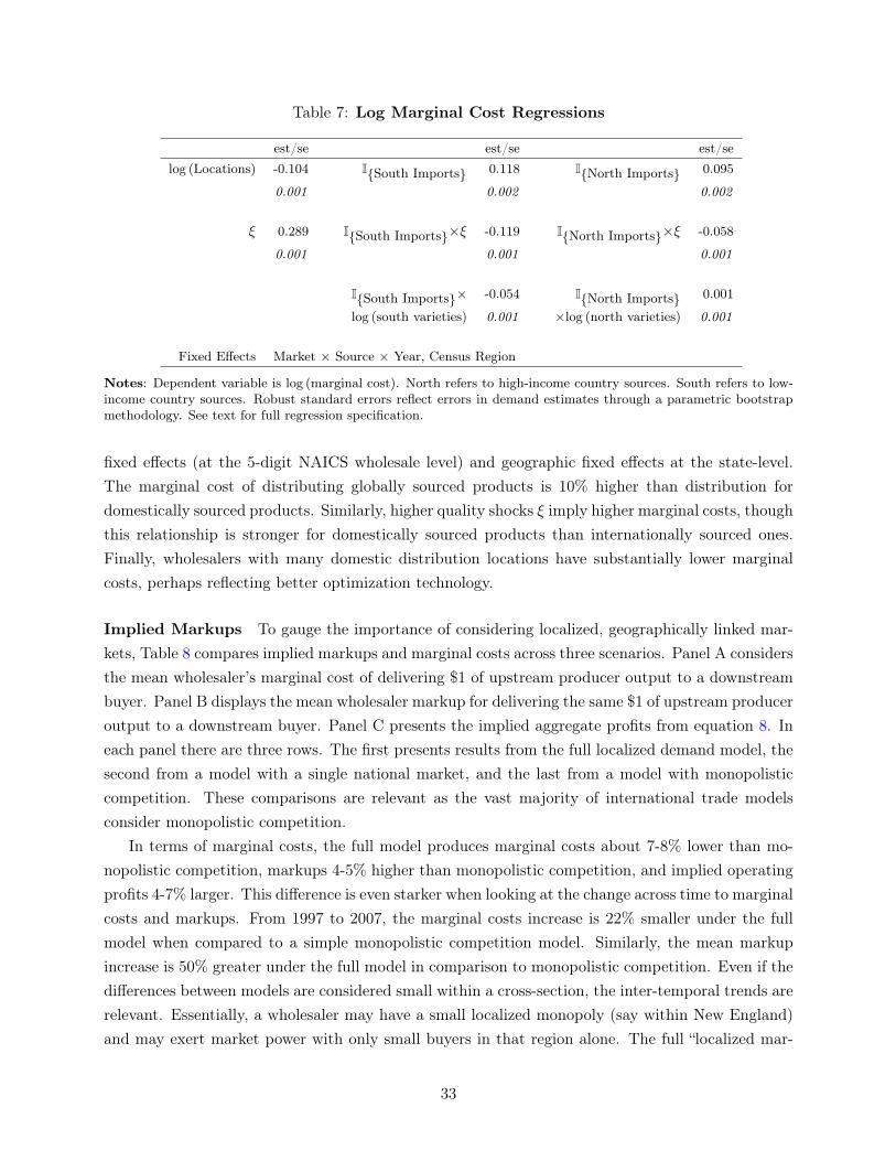
Table 7: Log Marginal Cost Regressions

est/se est/se est/selog (Locations) -0.104 I{South Imports} 0.118 I{North Imports} 0.095

0.001 0.002 0.002

⇠ 0.289 I{South Imports}⇥⇠ -0.119 I{North Imports}⇥⇠ -0.058

0.001 0.001 0.001

I{South Imports}⇥ -0.054 I{North Imports} 0.001

log (south varieties) 0.001 ⇥log (north varieties) 0.001

Fixed Effects Market ⇥ Source ⇥ Year, Census Region

Notes: Dependent variable is log (marginal cost). North refers to high-income country sources. South refers to low-income country sources. Robust standard errors reflect errors in demand estimates through a parametric bootstrapmethodology. See text for full regression specification.

fixed effects (at the 5-digit NAICS wholesale level) and geographic fixed effects at the state-level.The marginal cost of distributing globally sourced products is 10% higher than distribution fordomestically sourced products. Similarly, higher quality shocks ⇠ imply higher marginal costs, thoughthis relationship is stronger for domestically sourced products than internationally sourced ones.Finally, wholesalers with many domestic distribution locations have substantially lower marginalcosts, perhaps reflecting better optimization technology.

Implied Markups To gauge the importance of considering localized, geographically linked mar-kets, Table 8 compares implied markups and marginal costs across three scenarios. Panel A considersthe mean wholesaler’s marginal cost of delivering $1 of upstream producer output to a downstreambuyer. Panel B displays the mean wholesaler markup for delivering the same $1 of upstream produceroutput to a downstream buyer. Panel C presents the implied aggregate profits from equation 8. Ineach panel there are three rows. The first presents results from the full localized demand model, thesecond from a model with a single national market, and the last from a model with monopolisticcompetition. These comparisons are relevant as the vast majority of international trade modelsconsider monopolistic competition.

In terms of marginal costs, the full model produces marginal costs about 7-8% lower than mo-nopolistic competition, markups 4-5% higher than monopolistic competition, and implied operatingprofits 4-7% larger. This difference is even starker when looking at the change across time to marginalcosts and markups. From 1997 to 2007, the marginal costs increase is 22% smaller under the fullmodel when compared to a simple monopolistic competition model. Similarly, the mean markupincrease is 50% greater under the full model in comparison to monopolistic competition. Even if thedifferences between models are considered small within a cross-section, the inter-temporal trends arerelevant. Essentially, a wholesaler may have a small localized monopoly (say within New England)and may exert market power with only small buyers in that region alone. The full “localized mar-

33

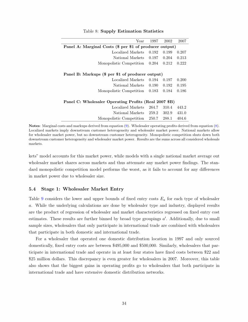
Table 8: Supply Estimation Statistics

Year 1997 2002 2007Panel A: Marginal Costs ($ per $1 of producer output)

Localized Markets 0.192 0.199 0.207National Markets 0.197 0.204 0.213

Monopolistic Competition 0.204 0.212 0.222

Panel B: Markups ($ per $1 of producer output)Localized Markets 0.194 0.197 0.200National Markets 0.190 0.192 0.195

Monopolistic Competition 0.183 0.184 0.186

Panel C: Wholesaler Operating Profits (Real 2007 $B)Localized Markets 264.7 310.4 443.2National Markets 259.2 302.9 431.0

Monopolistic Competition 250.7 288.1 404.6

Notes: Marginal costs and markups derived from equation (9). Wholesaler operating profits derived from equation (8).Localized markets imply downstream customer heterogeneity and wholesaler market power. National markets allowfor wholesaler market power, but no downstream customer heterogeneity. Monopolistic competition shuts down bothdownstream customer heterogeneity and wholesaler market power. Results are the sums across all considered wholesalemarkets.

kets” model accounts for this market power, while models with a single national market average outwholesaler market shares across markets and thus attenuate any market power findings. The stan-dard monopolistic competition model performs the worst, as it fails to account for any differencesin market power due to wholesaler size.

5.4 Stage 1: Wholesaler Market Entry

Table 9 considers the lower and upper bounds of fixed entry costs Ea for each type of wholesalera. While the underlying calculations are done by wholesaler type and industry, displayed resultsare the product of regression of wholesaler and market characteristics regressed on fixed entry costestimates. These results are further binned by broad type groupings a

0. Additionally, due to smallsample sizes, wholesalers that only participate in international trade are combined with wholesalersthat participate in both domestic and international trade.

For a wholesaler that operated one domestic distribution location in 1997 and only sourceddomestically, fixed entry costs are between $495,000 and $500,000. Similarly, wholesalers that par-ticipate in international trade and operate in at least four states have fixed costs between $22 and$25 million dollars. This discrepancy is even greater for wholesalers in 2007. Moreover, this tablealso shows that the biggest gains in operating profits go to wholesalers that both participate ininternational trade and have extensive domestic distribution networks.

34

Table 9: Average Entry Costs Across Product Markets (’000 2007 Dollars)

Year 1997 2007

Wholesaler type /# of Locations

DomesticDistributor

InternationalImporter

DomesticDistributor

InternationalImporter

One State [$495 500] [1,046 1,076] [629 638] [1,398 1,462]

Two States [3,098 3,142] [3,903 4,137] [4,042 4,113] [5,040 5,386]

Three States [4,485 4,546] [6,285 6,808] [8,473 8,772] [11,870 13,700]

Four-Six States [8,963 9,189] [9,285 9,895] [15,080 15,660] [23,740 28,140]

Seven+ States [36,910 38,880] [36,630 40,820] [39,820 42,470] [51,180 57,050]

Notes: Each cell displays bounds for fixed entry costs. Results are the product of regression of wholesaler and marketcharacteristics regressed on fixed entry cost estimates.

Table 10: Increasing in Returns to Scale + Global Sourcing:Change in Operating Profits from 1997 to 2007

Wholesaler Type

Number of DistributionWarehouses

DomesticDistributor

InternationalImporter

One State 28% 36%

Two States 31% 30%

Three States 93% 101%

Four-Six States 70% 184%

Notes: Each cell displays the percentage change in real operating profits for the average firm between 1997 and 2007.

Complementarity Between International Trade and Distribution Network Expansion

Table 10 quantifies both the increasing returns to scale over time and the complementarity betweenthe number of wholesaler distribution warehouses and global sourcing. This table displays wholesaleroperating profits, averaged across industries and binned by wholesaler types. From 1997 to 2007,a wholesaler with only one distribution center that sources only domestic products saw operatingprofits increase only 28%. An otherwise similar wholesaler, but that also sourced products fromabroad saw profits increase 36%. A wholesaler that sources only domestic products, but operatesa domestic distribution network with a presence in four or more states saw profits increase 70%.However, a wholesaler that (a) imports products and (b) operates a domestic distribution networkpresent in four or more states, saw real operating profits more than double, increasing 184%. It isthis complementarity that both motivates and underpins the results in the counterfactuals.44

44Statistics are not computed for wholesalers that distribute in seven or more states, as there are compositionalchanges, along with small sample sizes; this renders direct comparison with other groups problematic.

35

Figure 5: Wholesaler Growth Decomposition

28% 30% 32% 34% 36% 38% 40% 42% 44%

Average 1997MarketShare

ChangesinWholesalerPrices

ChangesinInternationalSourcing

ChangesinDomesticDistributionNetwork

ChangesinDomesticSourcing

ChangesinFirmCount

Average 2007MarketShare

WholesalerMarketShares

Notes: This chart decomposes changes to the market shares of wholesalers versus direct distribution from 1997to 2007. In terms of interpretation, the topmost bar represents the market share of wholesalers in 1997. The redsecond line indicates if wholesaler prices in 1997 reflect wholesaler prices in 2007, wholesale market share would beapproximately 2 percentage points lower. The third green line indicates that if wholesaler distribution networks in1997 resembled wholesaler distribution networks in 2007, wholesaler market share would be 3 percentage points higher.Similar calculations take place for changes in domestic sourcing quality, international sourcing quality and wholesalernumbers. Data is aggregated across markets and normalized to account for changes in market sizes.

6 Growth Decomposition

The probability of a buyer sourcing from a wholesaler has increased about 35% from 1997 to 2007,even though the number of wholesalers has fallen. There are multiple channels to decompose outbuyer gains from wholesaling. These include changes in buyer types, wholesaler varieties, prices,economies of scale and quality (which can be further decomposed into gains from domestic andinternational sourcing strategies), and local product availability. What are the relative importanceof each of these channels? Table 11 and Figure 5 decompose these gains through the lens of thedemand and pricing models.

Table 11 nets out difference in the distribution of downstream buyers45 and considers changes infour categories; price effects, domestic distribution networks, domestic and international sourcing,and the variety of wholesalers. Column (1) displays these results considering the average of theseeffects across all sample markets. These changes are further broken down according to the size ofthe wholesalers. The column sums to 100%, accounting for the total change in wholesaler marketshare from 1997 to 2007. Columns (2), (3), and (4) consider the smallest 90% of wholesalers, the

45Formally, counterfactuals are run considering only the composition of buyers in 2007; the changes in wholesalermarket shares due to changes the composition of buyers in 1997 is netted out. In addition, as the underlyingcounterfactual decompositions do not linearly sum up to 100% as effects can interact both positively and negatively,the data presented data is normalized as to sum to 100%. Non-normalized figures are available on request.

36

Table 11: Decomposition of Shift to Wholesaling from 1997 to 2007

Wholesale Firm Percentile

AllFirms

Bottom90% 90-99% Top 1%

(1) (2) (3) (4)Aggregate 100.0% 12.1% 29.0% 63.5%

Gains Due To Price Effects -14.9% 1.0% -2.2% -13.7%Due To Changes in Marginal Costs -12.7% 0.8% -1.7% -11.9%Due To Changes in Markups -2.2% 0.2% -0.5% -1.8%

Gains Due to Domestic Distribution 21.2% 0.5% 2.6% 18.2%Gains Due to Sourcing Quality 98.4% 10.7% 28.6% 59.1%

Due to Domestic Sourcing 64.4% 7.6% 19.0% 37.8%Due to International Sourcing 33.9% 3.0% 9.6% 21.3%

Gains Due To Variety (Logit/CES Taste) -4.6%Notes: This table decomposes changes to the market shares of wholesaler distribution versus direct distribution from1997 to 2007. In terms of interpretation, the topmost line represents the percentage of change in market shares ofwholesaler in 1997 to 2007. Changes in the quality and number of the smallest 90% of wholesalers account for 12% ofthe change. Similarly changes in the quality and number of the top 1% of wholesalers account for 64% of the changein wholesaler market shares. The next eight lines decomposes this by various changes to wholesaling from 1997 to2007. For example the first column of the second line states that wholesaler market share in 1997 would be 15%smaller than the observed wholesale market share if wholesalers charged prices similar to 2007. . Data is averagedacross markets and normalized to account for changes in market sizes.

middle 90-99% of wholesalers, and the largest 1% of wholesalers respectively. Figure 5 presentsthe aggregate results graphically. Positive numbers indicate changes that are surplus enhancing forbuyers and negative numbers indicate changes that are surplus reducing.

The first channel considers changes in prices, which are decomposed into changes in markupsand marginal costs. As average wholesaler prices increase, this effect works against an increase inwholesaler market share. If 1997 wholesaler prices were offered in 2007, the increase in wholesalermarket share would be 15 percent larger. This change is driven by both increases in marginalcosts and changes in markups. As shown in Section 5 and Table 7, both internationally sourcedproducts and high quality domestic distribution incur higher marginal costs. While smaller incomparison, markups also increase, reflecting increased market power, primarily for the largest 1%of wholesalers.46

The second channel reflects changes in domestic distribution networks due to more comprehensiveregional and national warehouse location choices. This accounts for a quarter of the total gain inaggregate wholesaler market shares. In particular, the largest wholesalers have drastically scaled upin size and offer local distribution to a greater subset of domestic buyers.

The third channel considers the changes to the quality of domestic sourcing and international46Note, the demand estimates find that market power and marginal costs actually decrease for the smallest whole-

salers, reflecting a selection effect with the smallest inefficient wholesalers exiting the market. Markups do not increasemuch for the largest wholesalers as these wholesalers expand into new states, where they may not be large enough toexert enough market power.

37

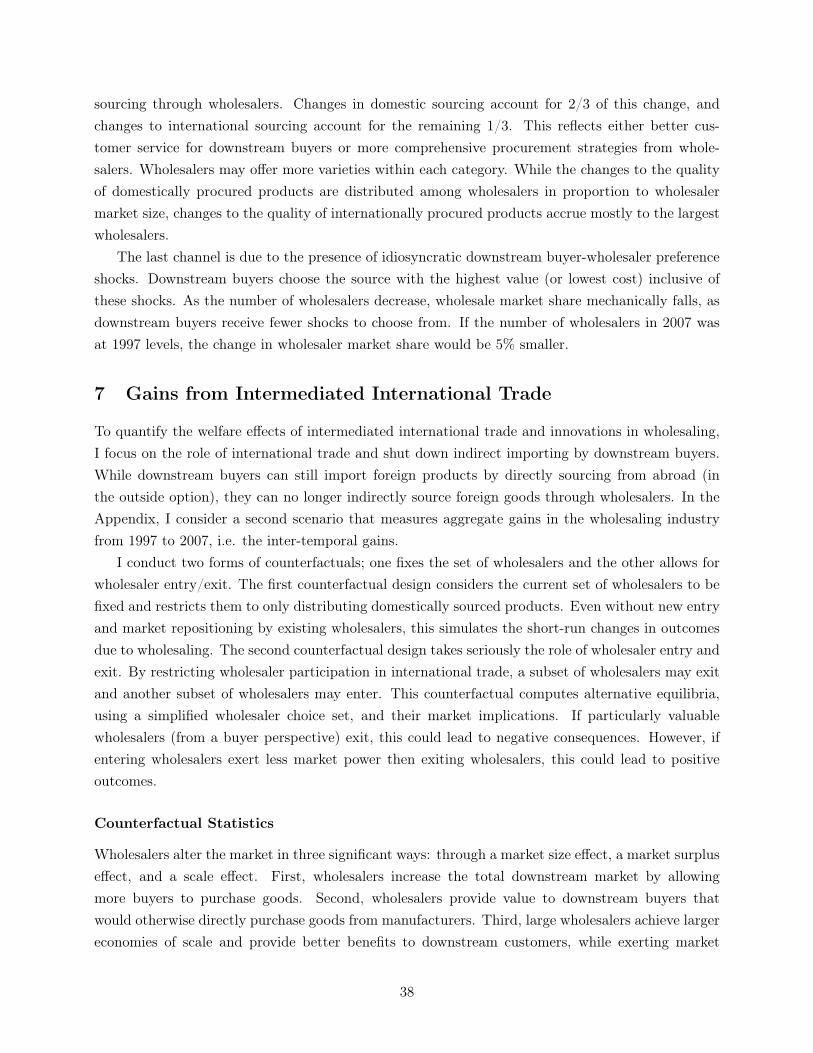
sourcing through wholesalers. Changes in domestic sourcing account for 2/3 of this change, andchanges to international sourcing account for the remaining 1/3. This reflects either better cus-tomer service for downstream buyers or more comprehensive procurement strategies from whole-salers. Wholesalers may offer more varieties within each category. While the changes to the qualityof domestically procured products are distributed among wholesalers in proportion to wholesalermarket size, changes to the quality of internationally procured products accrue mostly to the largestwholesalers.

The last channel is due to the presence of idiosyncratic downstream buyer-wholesaler preferenceshocks. Downstream buyers choose the source with the highest value (or lowest cost) inclusive ofthese shocks. As the number of wholesalers decrease, wholesale market share mechanically falls, asdownstream buyers receive fewer shocks to choose from. If the number of wholesalers in 2007 wasat 1997 levels, the change in wholesaler market share would be 5% smaller.

7 Gains from Intermediated International Trade

To quantify the welfare effects of intermediated international trade and innovations in wholesaling,I focus on the role of international trade and shut down indirect importing by downstream buyers.While downstream buyers can still import foreign products by directly sourcing from abroad (inthe outside option), they can no longer indirectly source foreign goods through wholesalers. In theAppendix, I consider a second scenario that measures aggregate gains in the wholesaling industryfrom 1997 to 2007, i.e. the inter-temporal gains.

I conduct two forms of counterfactuals; one fixes the set of wholesalers and the other allows forwholesaler entry/exit. The first counterfactual design considers the current set of wholesalers to befixed and restricts them to only distributing domestically sourced products. Even without new entryand market repositioning by existing wholesalers, this simulates the short-run changes in outcomesdue to wholesaling. The second counterfactual design takes seriously the role of wholesaler entry andexit. By restricting wholesaler participation in international trade, a subset of wholesalers may exitand another subset of wholesalers may enter. This counterfactual computes alternative equilibria,using a simplified wholesaler choice set, and their market implications. If particularly valuablewholesalers (from a buyer perspective) exit, this could lead to negative consequences. However, ifentering wholesalers exert less market power then exiting wholesalers, this could lead to positiveoutcomes.

Counterfactual Statistics

Wholesalers alter the market in three significant ways: through a market size effect, a market surpluseffect, and a scale effect. First, wholesalers increase the total downstream market by allowingmore buyers to purchase goods. Second, wholesalers provide value to downstream buyers thatwould otherwise directly purchase goods from manufacturers. Third, large wholesalers achieve largereconomies of scale and provide better benefits to downstream customers, while exerting market

38

Table 12: Surplus Changes from Intermediated International Trade

Baseline Counterfactual 1 Counterfactual 2

Static Gains Static + Entry/Exit

1997 2002 2007 1997 2002 2007 1997 2002 2007

Panel A: Levels

Number of Wholesalers 221,500 217,900 213,800 221,500 217,900 213,800 298,700 296,300 290,900

Number of Wholesalers/Market 3,955 3,891 3,818 3,955 3,891 3,818 5,334 5,291 5,195

Total Purchased Value $3,327 $3,385 $4,263 $3,276 $3,319 $4,144 $3,247 $3,269 $4,071

Average HHI 219.3 291.9 327.7 213.0 274.9 283.5 66.1 92.8 107.9

Wholesaler Mean Market Share 43% 49% 55% 40% 45% 50% 38% 43% 48%

Implied Markups 0.194 0.197 0.200 0.193 0.195 0.196 0.183 0.184 0.186

Panel B: Changes

� Downstream Surplus (bil) $131 $152 $222 $172 $220 $314

� Wholesaler Profits (bil) $3 $6 $7 $0 $0 $0

� Surplus + � Profits (bil) $134 $158 $228 $172 $220 $314

� Surplus/Purchased Value 4.1% 4.8% 5.5% 5.3% 6.7% 7.7%

� Market Size (bil) $51 $66 $119 $80 $116 $192

� Market Size/Purchased Value 1.5% 1.9% 2.8% 2.4% 3.4% 4.5%

Notes: Static gains are computed as the compensating variation needed to maintain the same expected utility for downstream customers, assuming no changesin the number, type or prices of wholesalers. Static gains allow wholesalers to change their prices in response to changes in their ability to source internationalvarieties. Entry/Exit gains allow wholesale firms to enter or exit the market due to changes in fixed costs and operating profits due to change in internationalsourcing. All figures in Billions of 2007 dollars.

39

power.

Market Size Gains The mechanism by which wholesalers increase the total market size is encom-passed by the aggregate downstream demand stage. As the expected utility of purchasing from awholesaler increases, existing downstream buyers will not only decide to purchase from a wholesaler,but new downstream purchasers will enter the market.

Surplus Gains I compute changes in the value of indirect sourcing to downstream buyers as wellas changes in wholesaler profits. Wholesalers can improve the downstream surplus of buyers thatalready purchase from wholesalers, or those that switch from purchasing directly from manufacturers.Through estimates of the indirect utility function in equation (1), I back out the monetary valuationof these changes. In addition, counterfactual wholesaler profits can be computed using the estimatedwholesaler fixed entry and market positioning costs.

Changes Due to Entry/Exit Wholesaler entry and exit can cause further shifts in both down-stream buyer surplus and wholesaler profits. Changes in the fixed cost of wholesaler entry, fromchanges in returns to scale, can lead to changes in the composition of wholesalers and their bene-fits to downstream firms. Previewing my findings, international trade allows for a large number ofhigh quality nation-wide wholesalers and nearly doubles the direct surplus gains from intermediatedinternational trade.

Counterfactual estimation is hard due to the difficulty (a) in finding all equilibria and (b) inchoosing the correct alternative equilibrium.47 As the entry and exit of wholesalers allows formany possible counterfactual equilibria, computation simplifies the choice set of entrants and theirdecisions. Instead of allowing for the full set of wholesaler choices a used in estimation, a simplifiedset a

0 will be used. In terms of the pricing game, wholesalers will have iterated best responsescalculated starting from their marginal costs.48 Wholesalers continue to (a) enter while expectedoperating profits are higher than fixed costs and (b) exit if operating profits do not cover fixed costs.

7.1 Counterfactual 1: Fixed Set of Wholesalers

Table 12 summarizes the market effects of indirect international sourcing under the two counterfac-tuals. The first set of columns presents baseline results for 1997, 2002, and 2007. The second setof columns, labeled “Counterfactual 1,” summarizes changes due to indirect international sourcing,

47Wholesalers must choose which of the 51 geographic locations to participate in, along with the choice to participatein both domestic and different forms of international sourcing. This produces 2

51 ⇥ 7 ⇡ 2 ⇥ 10

16 possibilities perwholesaler. The typical market has over 3000 wholesalers, so competitive effects across all these wholesalers must alsobe computed.

Solving for a single equilibrium, let alone establishing uniqueness is a Sisyphian task without further simplifyingassumptions. In terms of the single firm problem, Jia (2008) and Seim and Waldfogel (2013) make progress. However,these frameworks do not solve for the best solution in light of competitive behavior or more then two heterogenousfirms. Jia (2008) finds a solution that relies only on having one competitor, and Seim and Waldfogel (2013) heavilyrestrict the behavior of competitive firms by limiting heterogenity.

48This avoids the issue of multiple equilibria in pricing.

40

Figure 6: Increase in Buyer Surplus due to Intermediated International Trade

(a) 1997 (b) 2007

considering wholesaler price responses, but not wholesaler entry/exit decisions. The third set ofcolumns labeled “Counterfactual 2” allows for wholesaler entry/exit and is discussed in the nextsection. Panel A displays the results of each counterfactuals in levels. Panel B considers changes inwholesaler profits and changes in downstream buyer surplus.

In this scenario, as shown in Panel A, market size and wholesaler market shares slightly decreasein all three years. This reflects the value downstream buyers place on sourcing products from abroadthrough wholesalers. Wholesaler market share falls, as international sourcing is heavily concentratedin the largest wholesalers. This also causes a similar decrease in markups.

Panel B considers the changes in market outcomes. In 1997, the loss of indirect internationalsourcing by wholesalers would reflect a $131 billion loss in surplus (in 2007 dollars), or 4.1% of down-stream expenditures. Analogously in 2007, the loss would reflect a $222 billion decrease in surplus,or 5.5% of downstream expenditures.49 The last row in Panel B computes changes in downstreammarket size due to indirect international sourcing. In 1997, total manufactured good purchaseswould be $50 billion smaller, a 1.5% decrease, without indirect international sources. In 2007, therewould be $119 billion fewer downstream purchases of manufactured goods, a 2.8% decrease. Thesefigures can be further decomposed across types of downstream buyers, both geographically and bypurchase size.

Figure 6 displays the geographic distribution downstream of international-trade related changesto buyer surplus in 1997 and 2007. Details from 1997 are shown in Panel A and details from2007 are shown in Panel B. Figure 6 displays the change in downstream surplus as a percentage ofdownstream expenditures. In 2007, California, New Jersey, and Texas all show an approximately

49This figure assumes that the outside option - sourcing from manufacturers is unchanged. This discrete choiceframework is unable to distinguish what are the gains due to changes in the outside option, rather just changes relativeto the outside option.

41

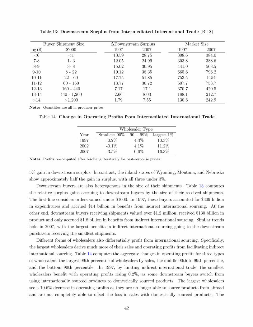
Table 13: Downstream Surplus from Intermediated International Trade (Bil $)

Buyer Shipment Size �Downstream Surplus Market Sizelog ($) $

0000 1997 2007 1997 2007

<6 <1 13.59 28.75 308.6 384.07-8 1- 3 12.05 24.99 303.8 388.68-9 3- 8 15.02 30.95 441.0 563.59-10 8 - 22 19.12 38.35 665.6 796.210-11 22 - 60 17.75 51.85 753.5 115411-12 60 - 160 13.77 30.72 607.7 753.712-13 160 - 440 7.17 17.1 370.7 420.513-14 440 - 1,200 2.66 8.03 188.1 212.7>14 >1,200 1.79 7.55 130.6 242.9

Notes: Quantities are all in producer prices.

Table 14: Change in Operating Profits from Intermediated International Trade

Wholesaler TypeYear Smallest 90% 90� 99% largest 1%

1997 -0.2% 4.3% 10.3%2002 -0.1% 4.1% 11.2%2007 -3.5% 0.6% 16.3%

Notes: Profits re-computed after resolving iteratively for best-response prices.

5% gain in downstream surplus. In contrast, the inland states of Wyoming, Montana, and Nebraskashow approximately half the gain in surplus, with all three under 3%.

Downstream buyers are also heterogenous in the size of their shipments. Table 13 computesthe relative surplus gains accruing to downstream buyers by the size of their received shipments.The first line considers orders valued under $1000. In 1997, these buyers accounted for $309 billionin expenditures and accrued $14 billion in benefits from indirect international sourcing. At theother end, downstream buyers receiving shipments valued over $1.2 million, received $130 billion inproduct and only accrued $1.8 billion in benefits from indirect international sourcing. Similar trendshold in 2007, with the largest benefits in indirect international sourcing going to the downstreampurchasers receiving the smallest shipments.

Different forms of wholesalers also differentially profit from international sourcing. Specifically,the largest wholesalers derive much more of their sales and operating profits from facilitating indirectinternational sourcing. Table 14 computes the aggregate changes in operating profits for three typesof wholesalers, the largest 99th percentile of wholesalers by sales, the middle 90th to 99th percentile,and the bottom 90th percentile. In 1997, by limiting indirect international trade, the smallestwholesalers benefit with operating profits rising 0.2%, as some downstream buyers switch fromusing internationally sourced products to domestically sourced products. The largest wholesalerssee a 10.6% decrease in operating profits as they are no longer able to source products from abroadand are not completely able to offset the loss in sales with domestically sourced products. The

42

Table 15: Wholesalers in Intermediated International Trade

Mean Wholesalers byMarket

Mean WholesalerMarket Share Mean Wholesaler HHI

Baseline AfterEntry/Exit Baseline After

Entry/Exit Baseline AfterEntry/Exit

1997 3,955 5,334 0.011% 0.008% 219.3 66.12002 3,891 5,291 0.013% 0.008% 291.9 92.82007 3,818 5,291 0.014% 0.009% 327.7 107.9

Notes: The first set of columns counts the number of wholesalers present in the median market before and afterwholesaler entry/exit. The second set of columns presents the average aggregate national market share for a wholesalerwithin their respective market. The last column presents the HHI of the wholesale industry, allowing for directsourcing.

results from 2007 follow the same pattern, but are larger in magnitude. The smallest wholesalerssee a 3.5% gain in operating profits, while the largest wholesalers face a 16.3% decline.

7.2 Counterfactual 2: Allowing Wholesaler Entry/Exit

This counterfactual offers an extremely simplified view of competition, with all wholesalers takingone of three configurations, either as a local wholesaler with only domestic sourcing, a globalizedwholesaler with only international sourcing, or as a hybrid wholesaler with both international anddomestic sourcing. In this scenario, the international-only wholesalers exit the market; they are nolonger able to source materials. The hybrid wholesaler no longer has to pay the market positioningcosts of international distribution, but loses sales from their earlier internationally sourced products.

Combining the data with this model’s estimated parameters, domestic source-only wholesalersare the smallest, with the lowest fixed entry costs and low expected qualities ⇠ and high marginalcosts ⌫. These domestic-only wholesalers also tend to have small, extremely local distributionnetworks, with only one distribution outlet. Hybrid domestic-international wholesalers have thelargest fixed entry costs, but the highest expected qualities and lowest marginal costs. These hybridwholesalers also frequently have large national distribution networks, with multiple geographicallydispersed distribution points.

As there are two types of remaining wholesalers, there may still be more than one equilibriumin the number of each wholesaler type. For example, there may be one domestic wholesaler andtwo hybrid wholesalers, or three domestic wholesalers and one hybrid. This analysis chooses theequilibrium with the greatest number of hybrid wholesalers. As the hybrid wholesalers have higherexpected qualities and lower marginal costs, such wholesalers can be considered large first-movers.50

In computation, I simulate market entry 50 times and use the lower bounds of fixed cost estimates.This allows for the most free entry and provides for the most conservative statistics.

Table 12 and Table 15 summarize market outcome changes from indirect international sourcing.50Alternative results are calculated with equilibria that provide for the greatest number of domestic only wholesalers.

While different in some of the wholesaler count statistics, overall surplus results are roughly similar.

43

In the third set of columns in Table 12 that are labeled “Counterfactual 2,” I show aggregate changesin downstream surplus, wholesaler profits, and market size after allowing for simplified wholesalerentry. International trade leads to increases of $172 billion in buyer surplus in 1997 and over $314 bil-lion in 2007. This is nearly 70% higher than the first counterfactual that limits wholesaler entry/exit.Market forces drive out the best wholesalers (i.e. those that had both domestic and internationallysourced products). However, the free entry condition allows more domestic-only wholesalers to enterthe market, partially compensating for the loss of wholesalers that source globally.

In Table 15, the counterfactual number of wholesalers and their mean market shares are presentedand compared to observed data. Broadly speaking, there are many more wholesalers, each with lowermarket share. In 1997, the typical wholesale market had 3,955 wholesalers; in the counterfactual, thisincreases about 34%. Simultaneously the average counterfactual wholesaler has 27% percent lowermarket share. These figures are larger for 2007, with 36% more wholesalers with, on average, 28% lessmarket share. Market concentration also changes, as shown in the third set of columns, intermediatedinternational trade allows for much higher concentrations, summarized by the Herfindahl–HirschmanIndex.

7.3 Alternative Scenario: Wholesaler Technology

In Appendix D, I consider a second scenario that measures aggregate gains in the wholesalingindustry from 1997 to 2007, i.e. the inter-temporal gains from wholesaler technology. Downstreambuyers in 2007 will no longer buy from the set of wholesalers from 2007, rather they will buy fromthe set of wholesalers using wholesaling technology from 1997. Summarizing my findings, changes inwholesaler technology and sourcing provide a yearly gain of $300 billion in total surplus, offsettinga $40 billion loss from increases in wholesaler market power.

8 Underlying Mechanisms Interpretations

While changes in the costs and benefits of international sourcing drive much of the observed evolutionin the wholesaling marketplace, this paper does not directly address the underlying mechanisms.This section provides a preliminary analysis. First, I discuss changes to the outside option, directlysourcing from a manufacturer. Second, I provide preliminary data concerning the use of informationtechnology in the wholesale sector.

All measurements to wholesaler quality are relative to the outside option, as are wholesaler prices.If domestic manufacturing is declining in quality or availability, downstream buyers will naturallysubstitute towards foreign suppliers, which may only be accessible through indirect sourcing. Sim-ilarly, changes in relative manufacturer’s prices across sources may change the relative valuation ofwholesaling versus direct sourcing. Further work, using both international trade data and domesticproduction data could provide new insights. Recent research (Bernard and Fort (2015) and Bernard,Smeets and Warzynski (2016)) and anecdotal evidence suggest that the rise in wholesalers may bedue to a economy-wide trend in former manufacturing firms closing domestic production operations

44

Figure 7: Share of Investment in Software

0.0

5.1

.15

1940 1960 1980 2000 2020year

Manufacturing Wholesale

Share on softwareInvestment expenditures

Source: BEA Investment Data

and only retaining design and distribution facilities. However, I find that these firms are not drivingmy results in Appendix E.

While this paper is able to bound the costs and the returns to scale for both internationalsourcing and domestic investment (and their complementarity), it does not discuses what technologyunderpins this change. Figure 7 provides preliminary and suggestive evidence that innovations andexpenditures on information technology (IT) may be driving these trends. This figure shows theshare of investment on software (an important component of IT) in both the manufacturing andwholesale sectors. While the share has increased at a similar rates from 1960 to 1995, the pathdiverged between 1995 and 2005. Today, software accounts for 13% of all investment by wholesalefirms, but less than 5% of investment by manufacturers. This finding corresponds favorably to mydata; however, showing causality requires further analysis and is part of a larger research agenda.

9 Conclusion

Wholesalers and intermediaries are critical to global and domestic supply chains. This paper es-tablishes a set of facts regarding wholesalers in relation to their upstream sources and downstreambuyers. The distribution of goods in the United States through wholesalers has substantially in-creased, with the very largest wholesalers both increasing their domestic distribution networks andsourcing more foreign products. These facts are combined with a demand model to estimate down-stream user preferences for intermediated trade through wholesalers. Wholesaler market entry isendogenized to consider counterfactuals regarding changes in fixed costs and the complementarityof a wholesaler’s international sourcing strategy with their domestic distribution network. The dataprovides evidence of trade-induced market power, where counterfactual wholesaler concentrationsand markups are lower in the absence of international trade. However, downstream buyers gain

45

substantial surplus from the expansion of the wholesale industry, which more than offsets increasesin wholesaler market power.

Globalization is a wedge that may allow for both (a) more market power and (b) widespreadbenefits. In the context of wholesaling, I find that benefits dominate changes in market power overthe last 20 years. However, this result is hard to generalize over other industries, time periods, orcontexts. This result stemmed from both the observed data and the model’s estimated parameters;different contexts will provide different results.

This paper provides one of the first comprehensive empirical studies of wholesaling and the roleit plays in both the global and domestic economies. However, there is wide scope for both extendingthis framework and examining various assumptions. In terms of expansion, future work could usea model of intermediation with heterogenous demand and place wholesalers in a tractable generalequilibrium framework to consider aggregate welfare changes. Alternatively, additional work shouldconsider changes in upstream manufacturing. Gains are all relative to sourcing directly from amanufacturer. Difficulty in sourcing from a manufacturer (both domestically and internationally)can offset gains from wholesaling. This paper also leads to questions that examine the boundaryof the firm: should a manufacturing firm expand domestic distribution networks, or outsource to awholesaler? Finally, this paper highlights the fruitful and productive work possible at the intersectionof industrial organization and international trade.

46

References

Abel-Koch, Jennifer, “Who Uses Intermediaries in International Trade? Evidence from Firm-level Survey Data,”The World Economy, 2013, 36 (8), 1041–1064.

Ackerberg, Daniel, C Lanier Benkard, Steven Berry, and Ariel Pakes, “Econometric tools for analyzingmarket outcomes,” Handbook of econometrics, 2007, 6, 4171–4276.

Ahn, JaeBin, Amit K Khandelwal, and Shang-Jin Wei, “The role of intermediaries in facilitating trade,”Journal of International Economics, 2011, 84 (1), 73–85.

Akerman, Anders, “A theory on the role of wholesalers in international trade based on economies of scope,” ResearchPapers in Economics, 2010, 1.

Anderson, Simon P, Andre De Palma, and Jacques François Thisse, Discrete choice theory of productdifferentiation, MIT press, 1992.

Andrews, Donald WK and Gustavo Soares, “Inference for parameters defined by moment inequalities usinggeneralized moment selection,” Econometrica, 2010, 78 (1), 119–157.

and Panle Jia Barwick, “Inference for parameters defined by moment inequalities: A recommended momentselection procedure,” Econometrica, 2012, 80 (6), 2805–2826.

Antràs, Pol and Arnaud Costinot, “Intermediated Trade,” Quarterly Journal of Economics, 2011, 126 (3), 1319–1374.

, Teresa C. Fort, and Felix Tintelnot, “The Margins of Global Sourcing: Theory and Evidence from U.S.Firms,” Working Paper 20772, National Bureau of Economic Research December 2014.

Arkolakis, Costas, “Market Penetration Costs and the New Consumers Margin in International Trade,” Journal ofpolitical economy, 2010, 118 (6), 1151–1199.

Atkin, David and Dave Donaldson, “Who’s getting globalized? the size and nature of intranational trade costs,”mimeo, 2012.

Bar-Isaac, Heski and Alessandro Gavazza, “Brokers’ contractual arrangements in the Manhattan residentialrental market,” Journal of Urban Economics, 2015, 86, 73–82.

Barger, Harold, Distribution’s Place in the American Economy Since 1869, NBER, 1955.

Bernard, Andrew B. and Teresa C. Fort, “Factoryless Goods Producing Firms,” American Economic Review:Papers and Proceedings, May 2015, 105 (5), 518–23.

Bernard, Andrew B, J Bradford Jensen, Stephen J Redding, and Peter K Schott, “Wholesalers andretailers in US trade (long version),” National Bureau of Economic Research Working Paper, 2010.

, Marco Grazzi, and Chiara Tomasi, “Intermediaries in international trade: Direct versus indirect modes ofexport,” National Bureau of Economic Research Working Paper, 2011.

Bernard, Andrew B., Valerie Smeets, and Frederic Warzynski, “Rethinking Deindustrialization,” WorkingPaper 22114, National Bureau of Economic Research March 2016.

Berry, Steven, Alon Eizenberg, and Joel Waldfogel, “Optimal product variety in radio markets,” TechnicalReport, National Bureau of Economic Research 2015.

and Peter Reiss, “Empirical models of entry and market structure,” Handbook of industrial organization, 2007,3, 1845–1886.

, James Levinsohn, and Ariel Pakes, “Automobile prices in market equilibrium,” Econometrica: Journal ofthe Econometric Society, 1995, pp. 841–890.

47

Berry, Steven T, “Estimating discrete-choice models of product differentiation,” The RAND Journal of Economics,1994, pp. 242–262.

Berry, Steven T. and Philip A. Haile, “Identification in Differentiated Products Markets Using Market LevelData,” Econometrica, 2014, 82 (5), 1749–1797.

Biglaiser, Gary, “Middlemen as experts,” The RAND journal of Economics, 1993, pp. 212–223.

and James W Friedman, “Middlemen as guarantors of quality,” International journal of industrial organization,1994, 12 (4), 509–531.

Blaum, Joaquin, Claire Lelarge, and Michael Peters, “The gains from input trade in firm-based models ofimporting,” Technical Report, National Bureau of Economic Research 2015.

Bresnahan, Timothy F, Scott Stern, and Manuel Trajtenberg, “Market Segmentation and the Sources ofRents from Innovation: Personal Computers in the Late 1980s,” The RAND Journal of Economics, 1997, 28,S17–S44.

Caplin, Andrew and Barry Nalebuff, “Aggregation and Imperfect Competition: On the Existence of Equilibrium,”Econometrica, January 1991, 59 (1), 25–59.

Cardell, N Scott, “Variance components structures for the extreme-value and logistic distributions with applicationto models of heterogeneity,” Econometric Theory, 1997, 13 (02), 185–213.

Chernozhukov, Victor, Han Hong, and Elie Tamer, “Estimation and Confidence Regions for Parameter Setsin Econometric Models1,” Econometrica, 2007, 75 (5), 1243–1284.

Crozet, Matthieu, Guy Lalanne, and Sandra Poncet, “Wholesalers in international trade,” European EconomicReview, 2013, 58, 1–17.

Davis, Peter, “Spatial competition in retail markets: movie theaters,” The RAND Journal of Economics, 2006, 37(4), 964–982.

De Loecker, Jan, “Product differentiation, multiproduct firms, and estimating the impact of trade liberalization onproductivity,” Econometrica, 2011, 79 (5), 1407–1451.

and Johannes Van Biesebroeck, “Effect of International Competition on Firm Productivity and Market Power,”February 2016, (21994).

, Pinelopi K. Goldberg, Amit Khandelwal, and Nina Pavcnik, “Prices, Markups and Trade Reform,”Econometrica, Forthcoming.

Eizenberg, Alon, “Upstream innovation and product variety in the us home pc market,” The Review of EconomicStudies, 2014, 81 (3), 1003–1045.

Elser, Bernd, Udo Jung, and Yves Willers, “Opportunities in Chemical Distribution,” Technical Report, TheBoston Consulting Group 2010.

Feenstra, Robert C and Gordon H Hanson, “Intermediaries in Entrepot Trade: Hong Kong Re-Exports ofChinese Goods,” Journal of Economics & Management Strategy, 2004, 13 (1), 3–35.

Felbermayr, Gabriel and Benjamin Jung, “Trade Intermediation and the Organization of Exporters,” Review ofInternational Economics, 2011, 19 (4), 634–648.

Ganapati, “Connecting Production and Distribution: Linking Manufacturing and Wholesaling Data,” TechnicalReport, Yale University 2015.

Gavazza, Alessandro, “The role of trading frictions in real asset markets,” The American Economic Review, 2011,101 (4), 1106–1143.

Goldberg, Pinelopi Koujianou and Rebecca Hellerstein, “A structural approach to identifying the sources oflocal currency price stability,” The Review of Economic Studies, 2013, 80 (1), 175–210.

48

Gopinath, Gita and Brent Neiman, “Trade Adjustment and Productivity in Large Crises,” American EconomicReview, March 2014, 104 (3), 793–831.

, Pierre-Olivier Gourinchas, Chang-Tai Hsieh, and Nicholas Li, “International prices, costs, and markupdifferences,” The American Economic Review, 2011, 101 (6), 2450–2486.

Gorman, WM, “Two stage budgeting,” mimeo, from Separability and Aggregation: The Collected Works of W. M.Gorman, Volume I, 1970.

Halpern, László, Miklós Koren, and Adam Szeidl, “Imported Inputs and Productivity,” American EconomicReview, December 2015, 105 (12), 3660–3703.

Hausman, Jerry A, “Valuation of new goods under perfect and imperfect competition,” in “The economics of newgoods,” University of Chicago Press, 1996, pp. 207–248.

Hausman, Jerry A., Gregory K. Leonard, and Daniel McFadden, “A utility-consistent, combined discretechoice and count data model Assessing recreational use losses due to natural resource damage,” Journal of PublicEconomics, 1995, 56 (1), 1 – 30.

Hausman, Jerry, Gregory Leonard, and J Douglas Zona, “Competitive analysis with differenciated products,”Annales d’Economie et de Statistique, 1994, pp. 159–180.

Hendel, Igal, “Estimating multiple-discrete choice models: An application to computerization returns,” The Reviewof Economic Studies, 1999, 66 (2), 423–446.

Ho, Kate and Ariel Pakes, “Hospital choices, hospital prices and financial incentives to physicians,” TechnicalReport, National Bureau of Economic Research 2013.

Houde, Jean-François, “Spatial differentiation and vertical mergers in retail markets for gasoline,” The AmericanEconomic Review, 2012, pp. 2147–2182.

Jia, Panle, “What happens when Wal-Mart comes to town: An empirical analysis of the discount retailing industry,”Econometrica, 2008, pp. 1263–1316.

Jung, Udo, Rob Wolleswinkel, Christian Hoffman, and Adam Rothman, “Specialty Chemical Distribution-Market Update,” Technical Report, The Boston Consulting Group 2014.

, Stefan Scholz, Christian Hoffman, and Anna Sinemus, “The Growing Opportunity for Chemical Distrib-utors,” Technical Report, The Boston Consulting Group 2013.

Katz, Michael L, “Vertical contractual relations,” Handbook of industrial organization, 1989, 1, 655–721.

Krishna, Kala and Lena Sheveleva, “Wheat or Strawberries? Intermediated Trade with Limited Contracting.,”Technical Report, National Bureau of Economic Research 2014.

Lukach, Carl, “Univar Presentation - 2015 Barclays Industrial Distribution Forum,” 2015.

Manrai, Ajay K and Rick L Andrews, “Two-stage discrete choice models for scanner panel data: An assessmentof process and assumptions,” European Journal of Operational Research, 1998, 111 (2), 193 – 215.

McFadden, Daniel, “Conditional logit analysis of qualitative choice behavior,” 1973.

, “Econometric models for probabilistic choice among products,” Journal of Business, 1980, pp. S13–S29.

Melitz, Marc J, “The impact of trade on intra-industry reallocations and aggregate industry productivity,” Econo-metrica, 2003, 71 (6), 1695–1725.

Murry, Charles, “Advertising in vertical relationships: An equilibrium model of the automobile industry,” 2014.

Nakamura, Emi and Dawit Zerom, “Accounting for Incomplete Pass-Through,” The Review of Economic Studies,2010, 77 (3), 1192–1230.

Nevo, Aviv, “Measuring market power in the ready-to-eat cereal industry,” Econometrica, 2001, 69 (2), 307–342.

49

Pakes, A., J. Porter, Kate Ho, and Joy Ishii, “Moment Inequalities and Their Application,” Econometrica,2015, 83 (1), 315–334.

Pavcnik, Nina, “Trade liberalization, exit, and productivity improvements: Evidence from Chilean plants,” TheReview of Economic Studies, 2002, 69 (1), 245–276.

Petrin, Amil, “Quantifying the Benefits of New Products: The Case of the Minivan,” Journal of Political Economy,2002, 110 (4), 705–729.

Petropoulou, Dimitra, Information costs, networks and intermediation in international trade, Centre for EconomicPerformance, London School of Economics and Political Science, 2008.

Rauch, James E. and Joel Watson, “Network Intermediaries in International Trade,” Journal of Economics &Management Strategy, 2004, 13 (1), 69–93.

Ross, Thomas W, “Winners and Losers under the Robinson-Patman Act,” Journal of Law and Economics, October1984, 27 (2), 243–71.

Rubinstein, Ariel and Asher Wolinsky, “Middlemen,” The Quarterly Journal of Economics, 1987, pp. 581–594.

Salz, Tobias, “Intermediation and Competition in Search Markets: An Empirical Case Study,” NYU Working Paper,2015.

Seim, Katja, “An empirical model of firm entry with endogenous product-type choices,” RAND Journal of Economics,2006, pp. 619–640.

and Joel Waldfogel, “Public Monopoly and Economic Efficiency: Evidence from the Pennsylvania Liquor ControlBoard’s Entry Decisions,” The American Economic Review, 2013, 103 (2), 831–862.

Spulber, Daniel F, “Market making by price-setting firms,” The Review of Economic Studies, 1996, 63 (4), 559–580.

, “Market microstructure and intermediation,” The Journal of Economic Perspectives, 1996, pp. 135–152.

, Market microstructure: intermediaries and the theory of the firm, Cambridge University Press, 1999.

Sutton, John, Sunk costs and market structure: Price competition, advertising, and the evolution of concentration,MIT press, 1991.

, Technology and market structure: theory and history, Mit Press, 2001.

Tang, Heiwai and Yifan Zhang, “Quality differentiation and trade intermediation,” Available at SSRN 2368660,2012.

The Economist, “Business in America - Too much of a good thing,” 2016.

Tirole, Jean, The theory of industrial organization, MIT press, 1988.

Townsend, Robert M., “Theories of intermediated structures,” Carnegie-Rochester Conference Series on PublicPolicy, 1983, 18 (0), 221 – 272.

Tsay, Andy A and Narendra Agrawal, “Modeling conflict and coordination in multi-channel distribution systems:A review,” in “Handbook of Quantitative Supply Chain Analysis,” Springer, 2004, pp. 557–606.

U.S. Department of Commerce, “Census of Manufactures,” Census Bureau, 1992-2012.

, “Census of Wholesale Trade,” Census Bureau, 1992-2012.

, “Commodity Flow Survey,” Census Bureau, 1992-2013.

, “Longitudinal Business Database,” Census Bureau, 1992-2013.

and Homeland Security, “Longitudinal Firm Trade Transaction Database,” Census Bureau and Customs, 1992-2012.

50

Villas-Boas, Sofia and Rebecca Hellerstein, “Identification of supply models of retailer and manufactureroligopoly pricing,” Economics Letters, 2006, 90 (1), 132–140.

Villas-Boas, Sofia Berto, “Vertical relationships between manufacturers and retailers: Inference with limited data,”The Review of Economic Studies, 2007, 74 (2), 625–652.

Wollman, Thomas, “Trucks Without Bailouts: Equilibrium Product Characteristics for Commercial Vehicles.” PhDdissertation, Harvard University 2014.

51

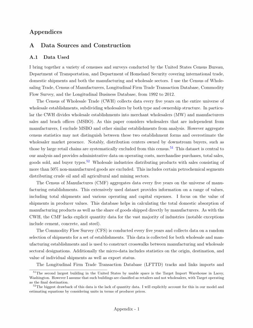
Appendices

A Data Sources and Construction

A.1 Data Used

I bring together a variety of censuses and surveys conducted by the United States Census Bureau,Department of Transportation, and Department of Homeland Security covering international trade,domestic shipments and both the manufacturing and wholesale sectors. I use the Census of Whole-saling Trade, Census of Manufacturers, Longitudinal Firm Trade Transaction Database, CommodityFlow Survey, and the Longitudinal Business Database, from 1992 to 2012.

The Census of Wholesale Trade (CWH) collects data every five years on the entire universe ofwholesale establishments, subdividing wholesalers by both type and ownership structure. In particu-lar the CWH divides wholesale establishments into merchant wholesalers (MW) and manufacturerssales and brach offices (MSBO). As this paper considers wholesalers that are independent frommanufacturers, I exclude MSBO and other similar establishments from analysis. However aggregatecensus statistics may not distinguish between these two establishment forms and overestimate thewholesaler market presence. Notably, distribution centers owned by downstream buyers, such asthose by large retail chains are systematically excluded from this census.51 This dataset is central toour analysis and provides administrative data on operating costs, merchandise purchases, total sales,goods sold, and buyer types.52 Wholesale industries distributing products with sales consisting ofmore than 50% non-manufactured goods are excluded. This includes certain petrochemical segmentsdistributing crude oil and all agricultural and mining sectors.

The Census of Manufactures (CMF) aggregates data every five years on the universe of manu-facturing establishments. This extensively used dataset provides information on a range of values,including total shipments and various operating and capital expenses. I focus on the value ofshipments in producer values. This database helps in calculating the total domestic absorption ofmanufacturing products as well as the share of goods shipped directly by manufacturers. As with theCWH, the CMF lacks explicit quantity data for the vast majority of industries (notable exceptionsinclude cement, concrete, and steel).

The Commodity Flow Survey (CFS) is conducted every five years and collects data on a randomselection of shipments for a set of establishments. This data is collected for both wholesale and man-ufacturing establishments and is used to construct crosswalks between manufacturing and wholesalesectoral designations. Additionally the micro-data includes statistics on the origin, destination, andvalue of individual shipments as well as export status.

The Longitudinal Firm Trade Transaction Database (LFTTD) tracks and links imports and51The second largest building in the United States by usable space is the Target Import Warehouse in Lacey,

Washington. However I assume that such buildings are classified as retailers and not wholesalers, with Target operatingas the final destination.

52The biggest drawback of this data is the lack of quantity data. I will explicitly account for this in our model andestimating equations by considering units in terms of producer prices.

Appendix - 1

exports by product at the firm level. This database catalogues all import and export transactionsby date from 1992 onwards in terms of both value and quantity. Tying all the datasets together, theLongitudinal Business Database provides a way to link individual establishments from the CWH,CMF, and CFS at the firm level, as well as linking these firms with trade data from the LFTTD.The process of merging these databases and further details are reported below.

A.2 Census of Wholesale Trade (CWH)

The US Census Defines a wholesaler in the 2007 North American Industry Classification System(NAICS) as:

The Wholesale Trade sector comprises establishments engaged in wholesaling mer-chandise, generally without transformation, and rendering services incidental to the saleof merchandise. The merchandise described in this sector includes the outputs of agri-culture, mining, manufacturing, and certain information industries, such as publishing.

The wholesaling process is an intermediate step in the distribution of merchandise.Wholesalers are organized to sell or arrange the purchase or sale of (a) goods for resale(i.e., goods sold to other wholesalers or retailers), (b) capital or durable non-consumergoods, and (c) raw and intermediate materials and supplies used in production.

Wholesalers sell merchandise to other businesses and normally operate from a ware-house or office. These warehouses and offices are characterized by having little or nodisplay of merchandise. In addition, neither the design nor the location of the premisesis intended to solicit walk-in traffic. Wholesalers do not normally use advertising directedto the general public. Customers are generally reached initially via telephone, in-personmarketing, or by specialized advertising that may include Internet and other electronicmeans. Follow-up orders are either vendor-initiated or client-initiated, generally basedon previous sales, and typically exhibit strong ties between sellers and buyers. In fact,transactions are often conducted between wholesalers and clients that have long-standingbusiness relationships.

This sector comprises two main types of wholesalers: merchant wholesalers that sellgoods on their own account and business to business electronic markets, agents, andbrokers that arrange sales and purchases for others generally for a commission or fee.

I focus on the first type of business, merchant wholesalers, which are further described as:

Merchant wholesale establishments typically maintain their own warehouse, wherethey receive and handle goods for their customers. Goods are generally sold withouttransformation, but may include integral functions, such as sorting, packaging, labeling,and other marketing services.

In addition, I omit two types of wholesalers, first those that are classified as Manufacturer’s Salesand Branch Offices (MSBO) and those that are classified as own-brand importers and markets. This

Appendix - 2

specifically excludes what Bernard and Fort (2015); Bernard et al. (2016) consider former manu-facturers that may have transitioned from domestic manufacturing into foreign manufacturing anddomestic distribution. If these firms are included as wholesalers, the wholesale shares of distributionincreases even more dramatically.

Wholesalers are classified according to their five-digit NAICS code. A market is defined as alldownstream buyers that buy and sell from these five-digit NAICS codes. For example, Code 42161refers to wholesalers participating in the resale of “Electrical Apparatus and Equipment, WiringSupplies and Construction Material”. While firms may appear to belong to multiple codes, thisproject only considers the Census-designated code. Future research projects may further exploremultiple-industry wholesalers.

Sales are aggregated considering the wholesaler’s purchase cost from their upstream source, netof export sales, and correcting for inventory adjustments. Prices are in manufacturers dollars andcomputed using the ratio between the sales to downstream buyers divided by upstream purchasesby the wholesalers. Wholesale industries that derive more than 50% of revenues from products thatare not manufactured are removed from analysis. These industries pertain primarily to mining andagricultural products. Additionally, NAICS sector 42471 and 42472 dealing with petroleum andpetroleum products are removed, as are NAICS sectors 42481, 42482, and 42494 that deal withbeer, wine and tobacco products. Petroleum products are removed due to the the industry takinga unique form due to the ownership and distribution of pipeline networks. Alcohol and tobaccoproducts are often regulated at the wholesaler level by individual states. Some states do not allowfor direct sourcing by downstream retailers and force the usage of wholesalers, rending my model ofwholesaling spurious.

A.2.1 Wholesaler Prices

Wholesaler prices are systematically denoted in producer prices. Therefore a wholesaler price of $1.3implies that it costs $1.3 to indirectly buy $1 manufactured output (at the “factory gate”).

Wholesalers prices pw are constructed as follows:

pw =

pwqw

pmqm,

where pm and pw represent the price paid by the wholesaler to a manufacturer and the price paid bya downstream firm to a wholesaler respectively. Variable qm represents the quantity purchased froma manufacturer, and qw represents the quantity sold by a wholesaler. In practice, quantity data isunavailable for most industries, so pmqm is approximated by

Cm = pmqm,

where Cm represents the expenditures of a wholesaler on manufactured goods. Similarly

Rw = pwqw,

Appendix - 3

where Rw represents the revenue of a wholesaler.I clean the data so wholesaler inventory changes are netted out, thus:

pw =

pw

pm.

As estimation requires a normalization, I set pm = 1, so wholesaler prices pw are all relative toproducer prices pm. I explore robustness to this price definition in Appendix B.3, where I allowdifferentiated buyers to face different wholesaler prices.

A.2.2 Wholesaler Sales Data

Wholesaler sales data is broken down by product origin by merging the LFTTD and CWH onfirm-level characteristics. First, total sales are derived from the line item referring to “Sales andoperating receipts.” Purchases from manufacturers are derived from the line referring to “Purchasesof merchandise for resale.”

Data from the LFTTD denotes the imports by country of origin. Countries are divided intotwo categories using the World Bank’s World Development Indicators Database from 1997. Sourceswith per-capita gross domestic product (GDP) over $10,000 are categorized as high-income sources.Sources with per-capita GDP under $10,000 are classified as low-income sources. The cut-off countyin my database is Slovenia, all countries richer than Slovenia are thus high-income sources. Dueto extensive literature highlighting the pass-through nature of Hong Kong’s economy (Feenstra andHanson (2004)), imports from Hong Kong and Macau are re-classified as Chinese imports.

As the World Bank estimates are not complete, I manually categorize a small subset of countries.Afghanistan, Iraq, Kosovo, Myanmar, Nauru, Sao Tome and Principe, South Sudan, Somalia, andTimor-Leste are classified as low income countries. San Marino is classified as a high income country.Overseas territories of the UK, Netherlands, and France are classified according to their parentcountry’s status (see Gibraltar, Curacao, and St. Martin/Sint Maarten).

Wholesaler purchases of domestic manufactured good are computed by subtracting imports fromtotal merchandise purchases for resale. Finally, sales are adjusted to only consider domestic buyers.I subtract the percentage of sales and purchases that are used for export shipments.

A.3 Outside Share (Direct Sourcing) Data Construction

Both the summary statistics in Section 2 and the estimation routine in Section 4, require the con-struction of the total downstream market size and the share of the downstream market not servedby US based wholesalers (the outside option). As wholesalers in the Census of Wholesale Firms(CWH) and and manufacturing producers in Census of Manufacturers (CMF) use different clas-sification systems, a series of NAICS Wholesale to NAICS Manufacturers code concordances areused. See Ganapati (2015) for an overview of the process. In addition, the Import-Export Database(LFTTD) uses the Harmonized System (HS) of good classification and the Commodity Flow Sur-vey (CFS) uses the Standardized Classification of Transported Goods (SCTG). Ganapati (2015)

Appendix - 4

also uses the micro-data in the CFS and the LFTTD to provide concordances between the variousNAICS, HS and SCTG codes at different levels of aggregation.

Total domestic absorption is computed as:

Total Domestic Absorption = Domestic Production

+International Imports

�International Exports.

Data on domestic production originates from the CMF as the sum of all domestically manufacturedproducts. Data on international imports and exports originates from the LFTTD. For domesticwholesalers in the LFTTD, values are deflated by average wholesaler markups over manufacturerprices. This produces “total domestic absorption” in terms of producer’s prices. Since manufac-turers and producers are not modeled in this paper, these prices are considered fixed. Alternativecomputation uses the CFS for domestic production and international export data.

Similarly domestic absorption accounted by wholesalers is computed as:

Domestic Wholsaler Absorption = Domestically Sourced Wholesaler Shipments

+Wholesaler Imports

�Wholesaler International Exports.

The first two components are computed using the combination of the CWH along with the LFTTD.The CWH reports total shipments and total exports, the LFTTD reports the total imports of afirm. Wholesaler international exports are computed using the self-reported CWH figure for totalexports, alternatively the LFTTD may also be used.

Table 2 aggregates these statistics across our entire sample. See the main text for further analysisand a summary.

A.4 Detailed Wholesaler Statistics

Tables A1-A4 highlight additional wholesaler statistics by wholesaler size.

A.5 Geographic Differentiation

In lieu of a continuous distance measure, this project discretizes downstream buyer location by USstates53, which are each located in 4 regions and 9 divisions. This project considers three distinctlevels of distance with regards to the downstream buyer, wholesaler that are located in the samestate, wholesaler located in the same census division and wholesalers located in the same censusdivision. Figure 8 displays these divisions.

53The District of Columbia is redefined as a state for this project.

Appendix - 5

Table A1: Wholesaler Margins and Accounting Costs by Market Share Quantile

Mean Wholesaler PricesShare Year

Quantile 1997 2002 20070-10 2.33 2.12 2.0110-20 1.95 1.84 1.8320-30 1.82 1.74 1.7430-40 1.74 1.69 1.6940-50 1.68 1.65 1.6350-60 1.63 1.60 1.5960-70 1.58 1.57 1.5570-80 1.54 1.53 1.5180-90 1.48 1.49 1.4890-99 1.41 1.43 1.43

99-99.5 1.35 1.38 1.3899.5+ 1.34 1.36 1.37

Mean Accounting CostsShare Year

Quantile 1997 2002 20070-10 1.32 1.08 0.9710-20 0.92 0.72 0.7120-30 0.77 0.61 0.6030-40 0.68 0.55 0.5440-50 0.61 0.51 0.4950-60 0.55 0.46 0.4560-70 0.49 0.43 0.4270-80 0.44 0.39 0.3880-90 0.38 0.35 0.3490-99 0.31 0.30 0.29

99-99.5 0.23 0.23 0.2399.5+ 0.19 0.20 0.19

Notes: Wholesaler margins calculated as Sales/Merchandise Purchases. Operating Costs calculated as OperatingExpenditures/Merchandise Purchases.

Table A2: Market Shares and Import Probabilities by Market Share Quantile

Market SharesShare Year

Quantile 1997 2002 20070-10 0.0001% 0.0001% 0.0001%10-20 0.0003% 0.0003% 0.0003%20-30 0.0006% 0.0006% 0.0005%30-40 0.0010% 0.0010% 0.0009%40-50 0.0015% 0.0015% 0.0013%50-60 0.0023% 0.0023% 0.0021%60-70 0.0036% 0.0035% 0.0033%70-80 0.0059% 0.0059% 0.0057%80-90 0.0114% 0.0115% 0.0114%90-99 0.0404% 0.0426% 0.0461%

99-99.5 0.1740% 0.1970% 0.2356%99.5+ 0.8241% 1.0197% 1.1335%

Import ProbabilitiesShare Year

Quantile 1997 2002 20070-10 5% 6% 8%10-20 6% 9% 10%20-30 9% 10% 13%30-40 11% 13% 16%40-50 13% 16% 19%50-60 15% 18% 22%60-70 19% 22% 26%70-80 23% 26% 30%80-90 27% 31% 36%90-99 39% 42% 48%

99-99.5 60% 62% 67%99.5+ 74% 78% 81%

Appendix - 6

Table A3: Prices and Average Costs by Market Share Quantile

Import CountriesShare Year

Quantile 1997 2002 20070-10 0.1 0.1 0.110-20 0.1 0.1 0.220-30 0.1 0.2 0.230-40 0.2 0.3 0.340-50 0.3 0.3 0.450-60 0.3 0.4 0.560-70 0.5 0.5 0.770-80 0.6 0.8 0.880-90 0.9 1.1 1.390-99 2.0 2.4 2.7

99-99.5 5.1 6.3 6.599.5+ 9.9 12.4 13.6

Import Country-ProductsShare Year

Quantile 1997 2002 20070-10 0.2 0.3 0.410-20 0.4 0.4 0.520-30 0.5 0.8 0.930-40 0.7 1.1 1.440-50 1.0 1.4 1.750-60 1.4 1.8 2.660-70 1.9 2.5 3.570-80 5.0 4.1 5.080-90 5.0 8.8 11.690-99 13.7 18.0 24.6

99-99.5 54.1 77.0 73.499.5+ 137.4 183.6 213.8

Table A4: Number of Locations by Market Share Quantile

Multi-location Firms by QuantileShare Year

Quantile 1997 2002 20070-10 0% 0% 0%10-20 0% 0% 0%20-30 0% 0% 1%30-40 1% 1% 1%40-50 1% 1% 2%50-60 2% 2% 3%60-70 4% 4% 4%70-80 7% 7% 7%80-90 13% 13% 14%90-99 28% 30% 31%

99-99.5 50% 53% 57%99.5+ 63% 68% 71%

Average Locations by QuantileShare Year

Quantile 1997 2002 20070-10 1.0 1.0 1.010-20 1.0 1.0 1.020-30 1.0 1.0 1.030-40 1.0 1.0 1.040-50 1.0 1.0 1.050-60 1.0 1.0 1.060-70 1.0 1.1 1.170-80 1.1 1.1 1.180-90 1.2 1.2 1.390-99 1.8 2.0 2.1

99-99.5 4.7 5.9 6.999.5+ 14.2 20.7 23.9

Appendix - 7

Figure 8: US Census Regions and Divisions

PANJ

NY

ME

NHVT

MA

CT RI

ND

SD

NE

KS

MN

IA

MO

IL

WI

INOH

MI

Census Regions and Divisions of the United States

PACIFIC

AK

0 200 400 Miles

TX

OK

AR

LA

MS ALGA

FL

SC

TNNC

KY

WVVA

MD

DC

DE

EASTNORTH

CENTRAL

MIDDLE

ATLANTIC

SOUTHATLANTICEAST

SOUTHCENTRAL

WESTSOUTH

CENTRAL

WESTNORTH

CENTRAL

0 200 400 Miles

HI

PACIFIC

0 100 200 Miles

WA

MT

WY

ID

OR

CA

NV

UT

CO

NM

AZ

MOUNTAIN

PACIFIC

WEST MIDWEST NORTHEAST

SOUTH

U.S. Department of Commerce Economics and Statistics Administration U.S. Census Bureau Prepared by the Geography Division

LEGEND

NEWENGLAND

REGIONDIVISIONSTATE

Appendix - 8

An alternative approach that would allow for tractable computation would be to map distancedirectly to distance indicator variables. This would prevent issues from considering the distancefrom New York to Connecticut differently than the distance from New York to New Jersey, dueto Census division classifications. Instead of considering buyers that are within the same censusdivision or region, the alternative would be to consider other states within pre-specified distancebands. For example, distance band 1 for New York would include all wholesalers in states that arereachable within 4 hours (250 miles) and distance band 2 would include all wholesalers in statesthat are within 8 hours (500 miles). Preliminary results show that estimates in Sections 5 and 6are largely consistent and the aggregate estimates in Section 7 are similar. However, the geographicbreakdown is slightly changed, with the welfare gains due to intermediation slightly rising in smallNew England and South Atlantic States (in particular Rhode Island and Delaware) and slightlyfalling in rural Mountain States (Wyoming and Montana).

B Demand Systems

This section provides micro-foundations for the indirect downstream profit functions used in Section3. This provides support for both the two-stage demand system and allows for simple extensions.While this specific toy demand model provides micro-foundations for the exact demand structurepresented in the main paper’s model, it is slightly generalizable, while still providing the neededstructure. There are two critical elements, first requiring a single-input invertible production functionand second requiring that the expectation of the marginal cost is sufficient for the wholesaler’sdecision in the last demand stage (in period t4) .54

B.1 Downstream Profit Maximization (1st Demand Stage)

To highlight the downstream buyers’s choice of purchase quantity before the realization of idiosyn-cratic match shocks, consider a hypothetical downstream buyer. Assume that these downstreambuyers produce output using a single input, such that output q = x, where q is the single input.Downstream buyers face constant elasticity of substitution (CES) demand for x > 0 units, withelasticity � > 1 and demand-shifter ⌘ > 0. Additionally suppose there are fixed cost of productionf drawn from some distribution F (·).

First, I solve the firm’s problem disregarding the fixed cost. Demand take the form:

x = ⌘p

��

Under such a CES demand framework, these downstream buyers charge markup µ which is a functionof the elasticity of substitution �:

µ =

�

� � 1

.

54The logic here closely follows Hausman et al. (1995), switching the buyer’s problem to consider a producer’s profitmaximization.

Appendix - 9

This markup is invariant of the demand shifter ⌘. The optimal price, p⇤, charged by such a down-stream buyer is product of the marginal cost of production mc and the markup µ:

p

⇤= mc · µ.

This price can be plugged back into the demand equation, solving for the optimal q⇤:

x

⇤= ⌘ (µ ·mc)

��.

Since the production function is one-to-one with the input, q⇤ = x

⇤. However, this assumes thatdownstream buyer marginal cost mc is known. In the two-stage decision, downstream buyers mustchoose q⇤⇤ in a first period, only with knowledge of the possible distribution of mc. Then in the secondperiod downstream buyers choose p

⇤⇤ to clear the market. Solving through backwards induction,conditional on x

⇤⇤, a downstream buyer chooses p

⇤⇤ such that:

p

⇤⇤=

✓x

⇤⇤

⌘

◆�1/�

Then in the first stage, a wholesaler solves:

maxE [(p (x)�mc)⇥ x]

Plugging in values, iterating expectations of marginal cost, and taking first order conditions:

⇡ (x) = x

✓x

⌘

◆�1/�

� xE [mc]

⇡

0(x) =

� � 1

�

✓x

⌘

◆�1/�

� E [mc]

Setting the first order conditions to zero and solving for x

⇤⇤:

x

⇤⇤= ⌘ (E [mc]µ)

��.

= q

⇤⇤

Where the last equality comes from the linear production function. This two stage demand providesfor the same prices and quantities as before, however allows for uncertainty in the realized marginalcost.

If the demand shifter ⌘ comes from some underlying distribution N (·), then the distribution ofq

⇤ will come from this same distribution scaled by (µ ·mc)

��.Revisiting fixed cost f , expected profits are:

E (⇡) = E ((p

⇤⇤ �mc) q

⇤⇤)� f = ⇡ (E (mc))� f

Appendix - 10

Where ⇡ is an increasing function in terms of the expected marginal cost. Production only occursif ⇡ � f > 0.

Aggregate downstream profits are decreasing function of marginal cost, thus a reduction inmarginal costs increases downstream profits.55 The second stages demand decision involves choosingthe optimal wholesaler to reduce this marginal cost. Additionally, these profits are a function ofthe fixed cost f ; lowered marginal costs imply that more firms will be able to enter the market.Aggregating across the draws for downstream demand ⌘ and the fixed costs f , this produces a massof buyers Mq that demand q units. If E (mc) falls, then the mass of Mq will shift upwards. Inmy model E (mc) is directly related to E

�¯

U

�, the expected utility of indirectly sourcing from a

wholesaler.

B.2 Downstream Cost Minimization (2nd Demand Stage)

The indirect downstream profit function can be micro-founded through a simple cost minimizationfunction for a downstream buyer. Suppose the cost of directly sourcing q units is:

Cdirect = qp0F (q)

Where p0 is the per-unit cost and F (q) is the per-unit overhead cost of setting up purchases for q

units.. Suppose the indirect cost of sourcing q units is:

Cindirect = qp1

Where p1 is the per-unit cost. For simplicity, suppose there isn’t an overhead cost. The logarithmof per-unit costs are then:

log

✓Cdirect

q

◆= log (p0) + log

✓F (q)

q

◆

log

✓Cindirect

q

◆= log (p1)

As long as downstream profits or utility are a function of the difference in per-unit costs, thenthe estimating equation (2) is appropriate.

B.3 Quantity discounts

Business to business transactions often take a form where the sale price is a function of the thequantity purchased. While estimated model does not directly account for this, a simple modificationallows for quantity discounts to be easily added, without changing the implication of the model.Suppose that wholesaler price p depends on the purchased quantity q through discount factor d (q)

and a mean price p:55Note that � > 1.

Appendix - 11

pq = p⇥ d (q) .

The discount function d (q) simply is a schedule that multiplies some baseline price conditional onthe purchase quantity q.

Simplifying the mean utility �q from equation (3) for any wholesaler selling to a buyer purchasingq units produces:

�q = ↵ log pq + f (q) + ⇠

Where f (q) represents the different preferences for wholesalers depending on purchase quantity q.Substituting our function for price, we obtain:

Uq = ↵ log p+ ↵ log d (q) + f (q)| {z }f(q)

+ ⇠

Instead of recovering f (q), estimation now recovers ˜

f (q). In terms of buyer welfare calculationsand market entry estimates, results are essentially unchanged. In terms of marginal cost estimates,similar logic prevails, and this paper computes a mean marginal cost, with industry-year fixed effectnetting out buyer compositional changes. However for counterfactuals, we assume that this discountstructure d (q), through ˜

f (q), is invariant. That is prices pq can only change through p and notthrough d (q), which will remain fixed.

B.4 Constant Elasticity of Substitution

The choice between wholesalers is modeled as a discrete choice decision and is micro-founded above.This modeling assumption is used both for tractability and realism, even though the majority ofinternational trade research uses a constant elasticity of substitution demand system. However,there is a nice link between CES demand systems and the discrete-choice logit demand systems, asfirst described by Anderson et al. (1992) and elaborated by De Loecker (2011).

Assume that downstream product demand takes the form:

D (p) =

⇣p

P

⌘�⇢⇠

Y

P

= (p)

�⇢⇠

Y

P

1�⇢

Where Y is total spending, ⇠ is a demand shifter, ⇢ is the elasticity of substitution, and the priceindex P takes the form:

P =

✓ˆ⇠p

1�⇢

◆ 11�⇢

Wholesaler profit maximization takes the following form:

⇡ = max

p(p� c)D (p) ,

Appendix - 12

which p denoting the price and c denoting wholesaler marginal cost. Assuming monopolistic com-petition, the optimization is as follows:

D (p) = � (p� c)D

0(p) = �

(p� c)

p

D(p)

p = c

⇢

(⇢� 1)

So then higher/lower prices due to ⇠ only operate through its correlation to c. Then wholesalerrevenues R are:

R = (p)

1�⇢⇠

Y

P

1�⇢

Taking a log transform of the wholesaler revenue function produces the relationship:

logR = (1� ⇢) log p+ log ⇠ + log

Y

P

1�⇢(19)

Now since revenues are related to market share s and total market size Y as R = sY , equation (19)can be rewritten as:

log s = (1� ⇢) log p+ log ⇠ � logP

1��

This estimating equation is almost identical to the logit estimating equation, with ↵p= (1� ⇢).

The difference between these models, as noted by Anderson et al. (1992), is clearly in the economicinterpretation, but the use of log prices forces identical substitution patterns. Note this model is notdirectly used in the empirical application, rather I use an aggregation of a nested logit framework.Further work can show this is equivalent to a two-level nested-CES demand aggregated across avariety of heterogenous downstream buyers. Both the two-level nested structure of demand and theheterogenous downstream buyers produce substantially more complex aggregate substitution pat-terns between wholesalers allowing much richer analysis. Critically, the difference between my modeland most international trade papers is in the supply-side. Firms do not compete monopolistically,they are allowed to exert variable market power.

B.5 Demand Estimation

B.5.1 Discrete Choice Estimation Routine

Estimation follows a Generalized Method of Moments technique in the vein of Petrin (2002) andmatches both aggregate national market shares and moments derived from the micro-level data.56

Assuming away buyer heterogeneity and allowing for one level of nests, I can derive the standardBerry (1994) estimation equation:

log sw,n/ log s0 = �w,n + �n log sw,n|n, (20)56Estimation proceeds sequentially, starting with demand estimation before moving to estimating the marginal cost

and market entry parameters.

Appendix - 13

where s0 represents the share of the outside option, sourcing directly from a manufacturer.57

With buyer heterogeneity, the aggregate market share equation is more elaborate:

log sw,n = log

X

j2J

hs0|j · s�w,n|j,n · exp (�w,n,j/ (1� �n))

iµj (21)

Variable s0|j represents the share of direct sourcing from manufacturing by buyers of type j andsw,n|j,n represents the conditional share of a wholesaler w selling in nest n to customer j. Withdownstream buyer heterogeneity, alongside wholesaler heterogeneity (that is different wholesalersserve different markets), the demand system provides for flexible substitution patterns and greatervariety in markups.

In practice the estimation uses a finite number of buyer types j, each with overall mass µj . Meanutility �w,n,j can be decomposed �w,n,j = �w,n +

˜

�w,n,j . The first component is common across alldownstream buyers and the second is specific to downstream buyers of type j. Solving for ⇠w,n,equation (21) is operationalized with one level of nests as:

⇠w,n = log sw,n�log

X

j2J

"s0,j

⇣~

�

⌘· s�w,n|j,n

⇣~

�

⌘· exp

˜

�w,n,j

1� �

!#µj�↵p

j log pw,n+↵ljIlw,j+↵

qjI

qw,j+aw,n↵

aj

(22)Where �w,n = ⇠w,n + ↵

pj log pw,n + aw,n↵

aj . This defines a contraction mapping from RN ! RN .

By recursively solving for ⇠w,n, I can solve this system of equations. Multiple levels of nests simplygeneralize this setup. Unlike the most general form in equation (21), the vector of parameters forunobservable coefficients is set such that ↵j = ↵ for all j 2 J .

In practice, this contraction mapping is the lengthiest step, as it is difficult to parallelize and re-quires 3 days of processing time the confidential census computing cluster. Alternative computationmethods such as Mathematical Programming with Equilibrium Constraints (MPEC) are similarlyslow as they require equality constraints for all 600,000 firms to be individually computed andchecked.

Aggregates Shares Using observed market shares, a candidate parameter estimate ✓, observedprices p and downstream market characteristics, estimation computes ⇠w,n (✓) for each wholesaler. Asshown in Section 4, ⇠w,n is uncorrelated with a series of instruments z, so our identifying restrictionis

E (⇠w,nzw,n) = 0

whose empirical analogue is Z

0⇠ (✓), where observations are stacked by wholesaler. This set of

assumptions will serve to pin down the price coefficient ↵ and substitution �.57If I assume that the unobserved parts of �w,n are mean zero, I can run a linear regression and recover ⇠w,n.

However, this means that a wholesaler based in New York will face the same demand in California as in New York,thus the model without buyer heterogeneity is a baseline for the full model.

Appendix - 14

Micro-Level Moments To pin down the coefficients for quantities and geographic indicators,estimation uses a series of moments that use estimated data and compare them with various facetsof our survey data. In particular, the estimation routine matches the shares of within metro-area,within state and within Census region wholesale shipments along with wholesale shipment sharesby shipment size. I denote the vector of moments produced by the data as mdata and the estimatedmoments as m (✓).

Moment Function Estimation obtains the parameter estimate ˆ

✓ from minimizing the followingcriterion equation:

ˆ

✓ = arg✓ minG (✓)

0WG (✓) , (23)

where

G (✓) =

"Z

0⇠ (✓)

mdata �m (✓)

#

and W is a weighting matrix. First stage identification uses the identity matrix. But in a two-step

procedure, estimation is iterated with the weighting matrix taking the form W2 =

G

⇣ˆ

✓1

⌘G

⇣ˆ

✓1

⌘0��1

with ˆ

✓1 denoting the estimates obtained using the identity weighting matrix.By using the relation, �w (�) = xw↵ + ⇠w, estimation can be simplified. Thus conditional on �,

the GMM routine can use the estimation:

↵IV (�) =

�X

0Z�Z

0X

��1 �X

0Z�Z

0X

��1�w (�;↵l,↵q)

Then I can use a GMM estimator to find �, ↵l and ↵q that minimize:

Jw (�;↵l,↵q) = [�w (�;↵l,↵q)� x↵w (�;↵l,↵q)]0Z�Z

0[�w (�;↵l,↵q)� x↵w (�;↵l,↵q)] .

B.5.2 Least-Squares Estimating Equation with Multi-Stage Nested Logit

In such a system, the market share of a wholesaler w, in nest n that sources from origin o (indirectforeign, indirect domestic, or direct sourcing) is

sw,n = sosn|osw,n|n.

Where sw,n is the overall market share, so is the market share of indirect foreign or indirect domesticsourcing, sn|o is the market share of a particular nest n conditional on source o. Assuming acorrelation structure parameterized by �s and �n, I can obtain the following market share equations(that generalize Berry (1994)):

ln

✓sw,n

s0

◆= �w,n + (�n) ln

�sw,n|n

�+ (�o) ln

�sn|o�.

Appendix - 15

Where �w,n is the mean valuation of wholesalers w’s product in nest n and s0 is the market share ofdirect sourcing from a manufacturer.

Similarly closed form demand elasticities can be obtained:

dsw,n

dpw,n=

↵

p

pw,nsw,n

⇢sw,n|n

⇢[1� so] sn|o +

1

1� �s

�1� sn|o

���+

1

1� �n

�1� sw,n|n

���

B.5.3 Demand Estimation

Formally, I identify the demand parameters ↵ and � using a modification of Berry and Haile (2014).Define X as the set of attributes defined in the first-stage of the entry game, before the realizationswholesaler quality ⇠ This means that a wholesaler has chosen whether they will participate in glob-alized trade and what dimension their domestic geographic footprint takes. Define Z as a set ofvariables that shift marginal cost, but not downstream buyer valuations of wholesaler products. De-fine M (↵,�) as a set of aggregate moments, such as the predicted share of local wholesale shipments,and where Md is the observed realization of these moments. I make the following assumptions:

Assumption 1 For every parameter (↵,�) there is at most one vector ⇠ such that sw,n (⇠w,n,↵,�)�s

0w,n = 0 for all (w, o) 2 W.

Assumption 2 E [⇠w,o|Z,X] = 0 for each (w, t) 2 W

Assumption 3 E [M (↵,�)�Md] = 0

These assumptions are standard from Berry et al. (1995) and Petrin (2002); a demand invertibilitycondition, an instrumental variable condition, and a set of aggregate moments. The first conditionallows us to invert the observed market shares, conditional on X and obtain mean valuation �w,n foreach wholesaler-product combination w, n 2 W.

Assumption 1, 2 and 3, along with the the structure imposed from the model and set of regularityconditions identify ⇠w,n with probability 1 and the function sw,n (�) is identified on �. Formally, evenwithout assuming a functional form for sw,n (·), demand identification stems from a modification ofBerry and Haile (2014) to allow for aggregate moments.

B.6 Demand Robustness

I consider two robustness exercises regarding my demand specification; (a) I compress and expandmy multi-level nested logit specification and (b) I consider parameter heterogeneity across product-markets. In general, I find that results are largely unchanged.

Multi-level Logit Demand In Figure 9, I show my baseline demand specification in panel (a)and an alternative demand specification in panel (b). Panel (b) compresses the top nesting structureinto the second nest. This implies that foreign-sourced products sold by multi-source wholesalersare similarly substitutable between foreign-sourced products sold by single-source wholesalers and

Appendix - 16

Figure 9: Downstream Buyer Sourcing Choice Trees

(a) Baseline

Downstream Buyer Choice

w1,d w2,d w2,f w3,f

Indirect Foreign

Indirect Domestic

Direct Sourcing

(A) (B) (C) (D)

(b) Alternative 1

Direct Sourcing

Downstream Buyer Choice

w1,d w2,d w2,f w3,f

(A) (B) (C) (D)

(c) Alternative 2

DomesticFactory

ForeignFactory

Direct Sourcing

Direct Sourcing

Downstream Buyer Choice

w1,d w2,d w2,f w3,f

(A) (B) (C) (D)

(d) Alternative 3

Downstream Buyer Choice

DomesticFactory

ForeignFactory

w1,d w2,d w2,f w3,f

Indirect Foreign

Indirect Domestic

Direct Sourcing

Direct Sourcing

(A) (B) (C) (D)

Notes: (A) refers to wholesalers that only source from domestic manufacturers. (B) and (C) refer to wholesalers thatbuy from both domestic and foreign sources, where (B) refers to their domestic purchases and (C) refers to theirforeign purchases. (D) refers to wholesalers that only source from abroad. The full model allows for two differenttypes of foreign sources, those from high-income countries and from low-income countries. Additionally, all directsourcing in lumped together in an outside option.

Appendix - 17

Table A5: Single-Level Logit Downstream Firm Choice Estimates

est/se est/se est/selog (price) -2.564 I{Same State} 3.367 log {Shipment Size} -0.333

0.023 0.045 0.003

I{# Locations>1} 0.199 I{Same Census Region} 1.340

0.005 0.082

�n 0.632 I{South Imports} -3.021 I{North Imports} -2.915

0.002 0.016 0.013

⇥log (south varieties) 0.704 ⇥log (north varieties) 0.7390.010 0.009

Fixed Effects Market ⇥ Source, Year ⇥ Source

Notes: Results from optimizing generalized method of moments (GMM) routine using a gradient search. RobustGMM standard errors presented. See text for full regression specification. North refers to high-income country sources.South refers to low-income country sources. These estimates are highly preliminary.

domestically-sourced products sold by multi-source wholesalers. Estimates from such a model areshown in Table A5. In general, this simplified model produces estimates slightly different from thebaseline model, as the coefficient estimates ↵ change to rationalize the data to difference in �.

Future projects will further explore the nesting structure in Panels (b) and (c). However thiswould require better data on the direct import-share of manufactured goods not at the national level,but at the local (state) level. This variation on the state-level import shares would help identifythe substitution parameter �direct that would govern the top-most nesting structure. However thiscurrent project aggregates all direct imports at the national level for a data-driven reason. The usedimport data often lists only the port of landing, not the final destination of an imported product.(As a hypothetical, a disproportionate number of auto parts land in New Jersey, relative to theshare auto plants located in the state.) Further work and assumptions are required disaggregate tostate-level shipments.

Parameter Heterogeneity In Table A6 I repeat the estimation of my model, however withineach of my 56 product-markets. This produces 56 estimates for the parameter vector (↵,�). I reportthe average of three critical values for my model and markup calculations, the price coefficient (↵p), and the two parameters governing substitution between nests (�o and �n). Results are similar tomy main pooled specifications.

C Markup Calculations

For simplicity in this Appendix, I assume one level of nests and derive markups when wholesalersexert market power. In terms of notation Qw,n denotes total sales by wholesaler w selling in nest

Appendix - 18

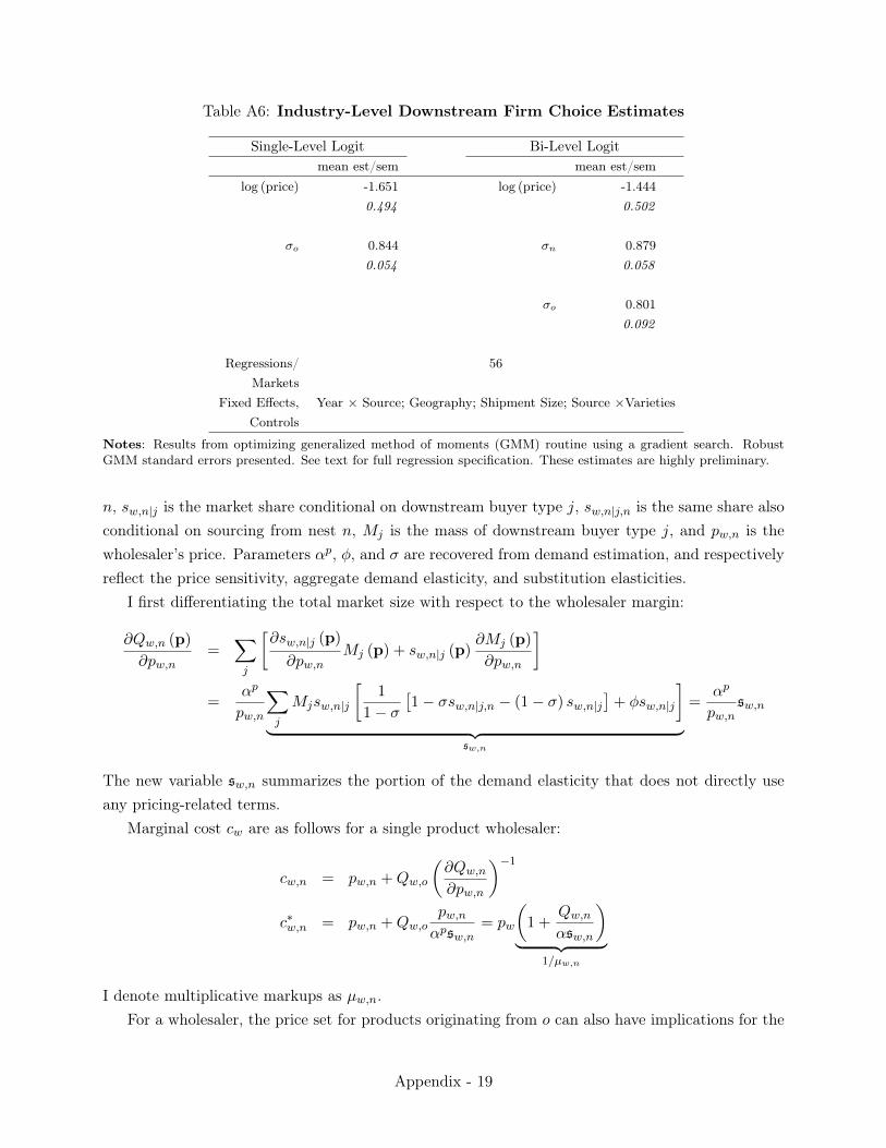
Table A6: Industry-Level Downstream Firm Choice Estimates

Single-Level Logit Bi-Level Logitmean est/sem mean est/sem

log (price) -1.651 log (price) -1.4440.494 0.502

�o 0.844 �n 0.8790.054 0.058

�o 0.8010.092

Regressions/Markets

56

Fixed Effects,Controls

Year ⇥ Source; Geography; Shipment Size; Source ⇥Varieties

Notes: Results from optimizing generalized method of moments (GMM) routine using a gradient search. RobustGMM standard errors presented. See text for full regression specification. These estimates are highly preliminary.

n, sw,n|j is the market share conditional on downstream buyer type j, sw,n|j,n is the same share alsoconditional on sourcing from nest n, Mj is the mass of downstream buyer type j, and pw,n is thewholesaler’s price. Parameters ↵p, �, and � are recovered from demand estimation, and respectivelyreflect the price sensitivity, aggregate demand elasticity, and substitution elasticities.

I first differentiating the total market size with respect to the wholesaler margin:

@Qw,n (p)

@pw,n=

X

j

@sw,n|j (p)

@pw,nMj (p) + sw,n|j (p)

@Mj (p)

@pw,n

�

=

↵

p

pw,n

X

j

Mjsw,n|j

1

1� �

⇥1� �sw,n|j,n � (1� �) sw,n|j

⇤+ �sw,n|j

�

| {z }sw,n

=

↵

p

pw,nsw,n

The new variable sw,n summarizes the portion of the demand elasticity that does not directly useany pricing-related terms.

Marginal cost cw are as follows for a single product wholesaler:

cw,n = pw,n +Qw,o

✓@Qw,n

@pw,n

◆�1

c

⇤w,n = pw,n +Qw,o

pw,n

↵

psw,n= pw

✓1 +

Qw,n

↵sw,n

◆

| {z }1/µw,n

I denote multiplicative markups as µw,n.For a wholesaler, the price set for products originating from o can also have implications for the

Appendix - 19

sales of products originating from n

0 where n 6= n

0:

@Qw,n0(p)

@pw,n=

X

j

@sw,n0|j (p)

@pw,nMj (p) + sw,n0|j (p)

@Mj (p)

@pw,n

�

=

↵

p

pw,n

X

j

Mjsw,n0|j (�� 1) sw,n|j

| {z }sn0,n

=

↵

hw,nsn0,n

For a multi-product wholesalers sourcing from multiple origins/selling in multiple nests n1, n2, ...,consider the matrix of partial derivatives of sales of each sold with respect to to the prices of boththe same product and other products sold:

� =

2

664

@Qw,n1@pw,n1

@Qw,n2@pw,n1

· · ·@Qw,n1@pw,n2

@Qw,n2

@pw,n2· · ·

...... . . .

3

775 = ↵

2

664

sn1,n1 sn2,n1 · · ·sn1,n2 sn2,n2 · · ·

...... . . .

3

775

2

664

1/pw,n1 0 · · ·0 1/pw,n2 · · ·...

... . . .

3

775

Solving the system of first order conditions implies that costs are:0

BB@

cw,n1

cw,n2

...

1

CCA =

0

BB@

pw,n1

pw,n2

...

1

CCA+�

�1

0

BB@

Qw,n1

Qw,n2

...

1

CCA

D Alternative Counterfactual: Intertemporal Comparison

This second scenario considers the aggregate gains in the wholesaling industry from 1997 to 2007, i.e.the inter-temporal gains. Downstream buyers in 2007 will no longer buy from the set of wholesalersfrom 2007, rather they will buy from the set of wholesalers using wholesaling technology from 1997.

D.1 Counterfactual 1: Fixed Set of Wholesalers

What is the net benefit to downstream buyers and wholesalers due to aggregate market changesfrom 1997 to 2007? As shown in Section 2, total indirect sourcing has increased 35% in marketshare and 98% in real shipments. Section 5 parses out these gains through the demand model andattributes these gains to various changes in the types of wholesalers. This section assesses the netvaluations of these changes by including both downstream buyer surplus and wholesaler profits.

Table A7 computes a variety of market outcomes by placing the universe of 1997 wholesalersin 2007. The first column lists a variety of relevant market outcomes, the number of wholesalerspresent, the number of wholesalers per market, the total market size for intermediate manufacturedgoods in producer prices, the change in downstream buyer surplus, the change in wholesaler profits,the sum of the changes in surplus and profits, and finally mean wholesaler market share (across

Appendix - 20

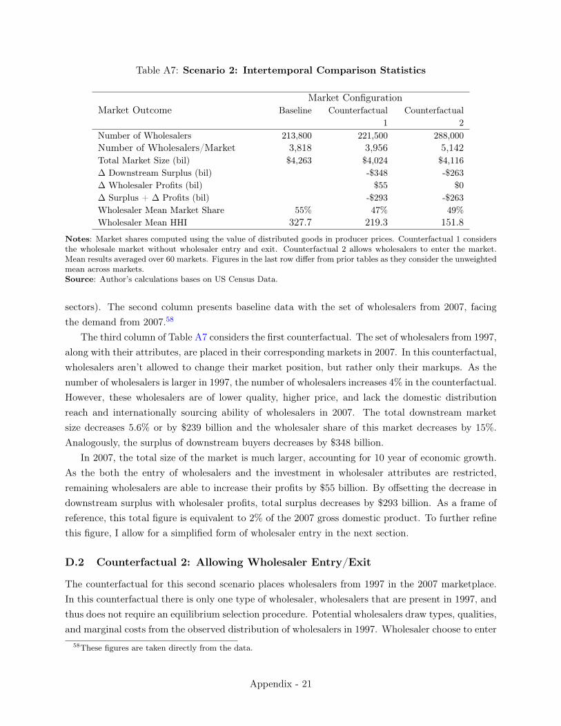
Table A7: Scenario 2: Intertemporal Comparison Statistics

Market ConfigurationMarket Outcome Baseline Counterfactual

1Counterfactual

2Number of Wholesalers 213,800 221,500 288,000Number of Wholesalers/Market 3,818 3,956 5,142Total Market Size (bil) $4,263 $4,024 $4,116� Downstream Surplus (bil) -$348 -$263� Wholesaler Profits (bil) $55 $0� Surplus + � Profits (bil) -$293 -$263Wholesaler Mean Market Share 55% 47% 49%Wholesaler Mean HHI 327.7 219.3 151.8

Notes: Market shares computed using the value of distributed goods in producer prices. Counterfactual 1 considersthe wholesale market without wholesaler entry and exit. Counterfactual 2 allows wholesalers to enter the market.Mean results averaged over 60 markets. Figures in the last row differ from prior tables as they consider the unweightedmean across markets.Source: Author’s calculations bases on US Census Data.

sectors). The second column presents baseline data with the set of wholesalers from 2007, facingthe demand from 2007.58

The third column of Table A7 considers the first counterfactual. The set of wholesalers from 1997,along with their attributes, are placed in their corresponding markets in 2007. In this counterfactual,wholesalers aren’t allowed to change their market position, but rather only their markups. As thenumber of wholesalers is larger in 1997, the number of wholesalers increases 4% in the counterfactual.However, these wholesalers are of lower quality, higher price, and lack the domestic distributionreach and internationally sourcing ability of wholesalers in 2007. The total downstream marketsize decreases 5.6% or by $239 billion and the wholesaler share of this market decreases by 15%.Analogously, the surplus of downstream buyers decreases by $348 billion.

In 2007, the total size of the market is much larger, accounting for 10 year of economic growth.As the both the entry of wholesalers and the investment in wholesaler attributes are restricted,remaining wholesalers are able to increase their profits by $55 billion. By offsetting the decrease indownstream surplus with wholesaler profits, total surplus decreases by $293 billion. As a frame ofreference, this total figure is equivalent to 2% of the 2007 gross domestic product. To further refinethis figure, I allow for a simplified form of wholesaler entry in the next section.

D.2 Counterfactual 2: Allowing Wholesaler Entry/Exit

The counterfactual for this second scenario places wholesalers from 1997 in the 2007 marketplace.In this counterfactual there is only one type of wholesaler, wholesalers that are present in 1997, andthus does not require an equilibrium selection procedure. Potential wholesalers draw types, qualities,and marginal costs from the observed distribution of wholesalers in 1997. Wholesaler choose to enter

58These figures are taken directly from the data.

Appendix - 21

if the expected profits from entry are greater then fixed costs and choose not to enter if expectedprofits are less than entry costs. Letting N denote the number of wholesalers in the market, thisimplies the following two conditions must hold:

EG

⇥⇡

2007(N + 1)

⇤< 0

EG

⇥⇡

2007(N)

⇤> 0

The function ⇡

2007(N) computes the profits by placing N wholesaler draws of (⇠, s, l) from the

distribution G (·) for wholesalers that were present in 1997. The expectation is then computedover this distribution G (·). This simulates counterfactual surplus if wholesalers compete away theirprofits through a free entry condition.

The third column of Table A7 computes changes in market outcomes relative to the observedset of wholesalers in 2007. If wholesaling technology from 1997 were placed in 2007, downstreamsurplus would decrease by $263 billion. Wholesaler profits would remain unchanged as the free entrycondition would force them to zero. The total downstream market for purchases would also decreaseby $170 billion, or 4%. In terms of wholesalers, aggregate wholesale market share would decrease 6percentage points, but the number of wholesalers would increase by one third, from 3,818 wholesalersper market to nearly 4,595 wholesalers. The individual market share of each wholesaler would alsodecrease by nearly 1/3, with a corresponding market concentration decrease.

E Factory-less good manufacturers

Recent research (Bernard and Fort, 2015; Bernard et al., 2016) and anecdotal evidence suggest thatthe rise in wholesalers may be due to a economy-wide trend in former manufacturing firms closingdomestic production operations and only retaining design and distribution facilities. It appears thetrends captured in this paper are largely independent and highly complementary to the findings inBernard and Fort (2015); Bernard et al. (2016). I address this research in three different ways. Firstthe residual quality term ⇠ may capture a portion of this change. Second, a large proportion of theseformer manufacturing firms are removed in the raw data. Third, the evidence from internationalsourcing patterns is inconsistent with common formulations of this outsourcing theory.

In the demand analysis the residual term ⇠w captures the quality of a wholesaler w that ra-tionalizes its price and market shares. If these wholesalers use contract manufacturing and thesecontract manufacturers produce products with higher qualities, then the trend towards factory-lessgood manufacturing is captured in this analysis. This is plausibly one of the underlying mechanismsthat deserves further study. However, it is not clear that these firms dominate the data.

The Census of Wholesalers includes categorizations such as “own-brand marketer” and “single-brand marketer”. If these wholesalers market only their own brand, then they are excluded from thesample of wholesalers and treated as manufacturers. A possible example could be the electronic firmApple, that markets its own products but outsources manufacturing.59 In addition, the analysis

59The exact categorizations of firms cannot be disclosed outside of the US Census Bureau, it is unclear where firms

Appendix - 22

also excludes manufacturer owned sales and branch offices. These locations exist to distributeproducts manufactured by a parent or sister firm. The elimination of these establishments doesreduce the observed growth in the wholesale sector, providing a conservative approach to measuringthe wholesaler market shares gains.

The behavior of the growth of these wholesalers takes a very particular form. As shown in tablesA2 and A4, the largest wholesalers are importing many more varieties from new foreign sources andsimultaneously increasing their distribution network within the United States. A common formula-tion of the factory-less good manufacturer theory is that these manufacturers close down productionin the United States and move manufacturing abroad, with little to say about designing new va-rieties for production or expanding local distribution networks. As the benefit from wholesalingprimarily derives from both sourcing new international destination, not just moving producing over-seas, and expanding domestic distribution, it is unclear that the shift to factory-less production isdriving the entirety of the trend towards wholesaling.

Finally, while this trend may be new for some firms, with Apple closing manufacturing lines inthe United States and outsourcing manufacturing to Foxconn in China, such ’factory-less’ producershave existed for a long time. Historically when IBM produced personal computers, they did notproduce all components sold with the IBM brand; the printer was simply a rebadged Epson deviceimported from Asia.60

F Endogenous Quality

In the main model, quality deviations ⇠ are exogenous. I propose a mechanism whereby ⇠ is endoge-nously chosen by firms. Suppose between Stage 1 and Stage 2, firms choose ⇠. Call this Stage 1.5.While theoretically easy to add, this stage presents estimation challenges and requires a modifiedestimation technique. In particular, this restricts the parameters estimated in the demand estima-tion stage. Instead of finding valuations for firm attributes aw,n, all attributes are subsumed in asingle vertical quality dimension ⇠. Therefore now:

�w,n = ↵pw,n + ⇠w,n.

F.1 Model Changes

Now, firms choose market entry in two stages. First wholesalers choose their domestic distributionlocations and between entering as firm with domestic sources, international sources or with bothdomestic and international sources. In the second stage firms choose the quality of their products,their internationally and domestically sourced varieties. This includes the variety of products awholesaler offers as well as the consumer service provided by the wholesaler. In terms of the model,a firm must optimally choose ⇠w,n for both their domestically and globally sourced products.

such as Apple stand and the textual discussion is purely hypothetical.60The IBM 5152 printer was a version of the Epson MX-80 printer

Appendix - 23

Conditioning on a firm’s type and location choices, the model assumes wholesaler w optimallychooses ⇠w,n for each product n 2 Nw. In particular they must invest fw (⇠) to receive productattributes ⇠w,n, which realize in operating profits ⇡w (⇠w,n) from equation (8). If a firm only par-ticipates in only domestic sourcing, they maximize the following problem by choosing their optimalfirm quality ⇠w,n :

max

⇠=[

⇠w,D,0,0]

⇡w (⇠)� fw (⇠) (24)

If firms participate in both first-world global and domestic markets, a firm w must choose twoparameters, ⇠w,n for n 2 {FH , D}, where n = FH represents first-world imports and n = D representsdomestically sourced products:

max

⇠=[

⇠w,D,⇠w,FH ]

⇡w (⇠)� fw (⇠) (25)

For simplicity, I now present results involving a single firm only involved in domestic sourcing andsuppress firm subscript w and product type subscript t. Conditional on location choices (marketentry), a firm’s first order maximization results in a first order conditions as ⇠ are both are optimallychosen:

d⇡ (⇠)

d⇠

=

df (⇠)

d⇠

(26)

Without any errors, this solution concept implies that any two ex-ante identical firms will choosethe same ⇠. As firms are only differentiated on an extremely limited set of dimensions in the marketentry stage, this setup will not fully rationalize the data. To better rationalize the data and accountfor the heterogeneity present in the world, the model allows for firm-specific investment cost shocks.Before wholesalers choose their market position, but after entering the market, each wholesalerreceives shocks to the marginal costs of investing. Call these shocks ⌘⇠.

Given these shocks, two ex-ante firms will no longer make the same investment choices andthus fully rationalize the observed data. Given a form for a time-varying investment function f (·),parameterized by the vector , the econometrician can recover changes in the return to investment.In particular, in the context of wholesaling, are the returns to investing in domestic and internationalquality differentially changing for large and small firms?

F.2 Estimation

In this model, unobserved downstream consumer valuations ⇠ are not exogenous shocks as in standarddiscrete choice models. They are the product of wholesale firm investments. This ⇠ is better writtenas ⇠ (a). This means that demand identification cannot identify a

aaw,n. In this case, all fixed effect,

a

aaw,n, and ⇠ are all subsumed by the new measure ⇠ (a). ⇠ (a) is no longer residual quality, it

is a complete measure of quality. Regardless, the coefficient ↵p can be identified as a cost shockhits a particular firm following their choice of a and ⇠ (a). In terms of ↵q, ↵l, and �; they arepartially identified off of aggregate moments. As ↵p is the only coefficient required to derive demandelasticities, estimation can proceed in a more restricted fashion.

Appendix - 24

Having made these assumptions, identification of this investment function proceeds directly fromthe first order conditions in equation (26). For any given company configuration a (that is conditionalon a company type s and location choices l), assume that the fixed costs of market positioning are:

f

aw (⇠, ⌘) =

✓

a1

a2

⌘w,⇠

◆exp (

a2⇠) + Ea

The function f

aw (⇠) measures the the cost of investing in quality ⇠ for wholesaler of configuration a.

There are scalar fixed costs Ea and two parameters, a1 and a

2 . Finally there is a wholesaler specificshock ⌘w,⇠. This structural investment cost shock is known to the firm, but not the econometrician.

Conditional on entry, a wholesale firm of configuration a seeks to maximize profits ⇡w (⇠) net ofinvestment fa

w (·). As both ⇡w (·) and f

cw (·) are smooth linear functions, computation of the optimal

profits requires solving the firm’s first order conditions. Marginal investment cost are

df

aw (⇠, ⌘)

d⇠

= (

a1⌘w,⇠) exp (

a2⇠)

and marginal profits stem from the first derivative of equation (8) with respect to ⇠, d⇡w (⇠) /d⇠. Asall the parameters in ⇡ (·) are known, the optimal marketing costs in equilibrium solve:

d⇡w (⇠)

d⇠

=

df

aw (⇠, ⌘)

d⇠

= (

a1⌘w,⇠) exp (

a2⇠) . (27)

Taking the logarithm of this equation produces the following relationship:

log

d⇡w (⇠)

d⇠

= log 1 + 2⇠ + log ⌘w,⇠. (28)

The relationship should be theoretically estimated by ordinary least squares, however the shock ⌘w,⇠

likely is correlated with the choice of ⇠. This echoes the endogeneity problem with ⇠ and hw inestimating equation (2). Estimation of requires a shifter of ⇠ that is uncorrelated with ⌘. Thisleads to an assumption required for identification.

Assumption 4 There exist Z⌘ such that E [⌘Z⌘] = 0.

Thus, under this model’s demand and supply systems, investment cost parameters are identi-fied.

What is a plausible exogenous shifter of ⇠? Estimation could use a combination of two shifters,one using the timing of the game and the second using geographic differentiation. The first shifteruses logic similar to those of the cost shifters in the demand estimation. Wholesale firms are likelyto choose higher levels of ⇠ when similar wholesale firms in nearby geographically proximate, butunrelated markets choose higher levels of ⇠. So the average ⇠ in New Haven for importing chemicalwholesalers can be used as an instrument for New Haven electronic wholesalers. The second shifterexploits the timing of the game, firms choose their attributes a before investing in ⇠, thus the numberof firms of type a

0 at the state, regional and national level shift the choice of ⇠ independently of ⌘.

Appendix - 25

In computation, ⇡w (⇠) is not fully known by a firm before the investment decision ⇠ is made.In particular there is an unobserved cost shock ⌫ from equation (14) that shifts profits. I assumethe distribution of ⌫ is known and firms maximize their expected profit. To aid in computation,instead of numerically integrating over ⌫, simulated draws of ⌫ are used to compute E [⇡w (⇠)]. Forsimplicity, I omit the expectation in what follows.

Investment function f

aw (·) is identified up to some fixed entry constant Ec. Following estimation

of a1 and

a2 , this step also generate the distributions G

a⌘ (·) for investment shocks of ⌘w,⇠. For

notational simplicity denote ⇠⇤w as the optimal choice for firm w with investment cost shocks ⌘.61

Second-stage net profits for a firm of configuration c are

na (⌘) = ⇡

aw (⇠

⇤(⌘))� ¯

f

aw (⇠

⇤(⌘) , ⌘) ,

where ¯

f

aw (·) = f

aw (·)� Ec.

Note that f (·) is only identified up to some constant Ea, ¯

f (·) subtracts this constant. Thefunction na (⌘) is used in the next stage to identify this entry cost Ea. For tractability, I assumethat fixed cost Ea is not paid in this stage, as firms in this stage have already entered into the marketand that an infinitesimally small investment in ⇠ (that is ⇠ ! �1) will realize a investment cost of0.62

F.3 Market Positioning Estimation

Table A8 presents estimation results for , which parameterizes the relationship between fixed costsand product quality ⇠. The table presents the results from two different regressions. The firstcolumn present the results for investment in quality regarding domestically sourced products andthe second column presents estimates for investment in sourcing internationally sourced products.All regressions control for year, industry and the domestic distribution networks of firms. Thisestimation uses a simplified demand system with only nesting at the product-source level and onlytwo types of products, domestically and internationally sourced.

The first three rows of Table A8 illustrate year-specific coefficients for 2 from equation (28).These estimates measure the cost in investing in quality ⇠domestic and ⇠international . The firstcolumn shows that it becomes more costly to invest in domestic sourcing quality over time. Oneinterpretation would be that there are fewer domestic manufacturers, and thus it is more difficultto find new and better domestic sources. Coefficient domestic

2 increases 7% from 1997 to 2007. Thesecond column shows that it has become less costly to invest in the quality of international sourcing,with

international2 decreasing 20% from 1997 to 2007. This may reflect both lowered trade barriers

and increases in the quality of foreign manufactured good sources, both of which make it easier to61The chosen functional form for fa

w (·) and the estimation equation (28) imply that 1⌘ is greater than zero, thusas long at 2 is greater than zero, fa

w (⇠⇤) will be always greater than zero.62Additionally, under a free entry condition for counterfactuals, estimates from this step are not needed to compute

alternative equilibria. Due to free entry, firms will reenter until ⇡0(⇠) = F 0

(⇠). This step does matter for when thefixed costs of entry change, but market positioning costs are unaltered. (are vice versa) In particular this step ismostly critical for understanding the role of ’business’ stealing arising from competition.

Appendix - 26

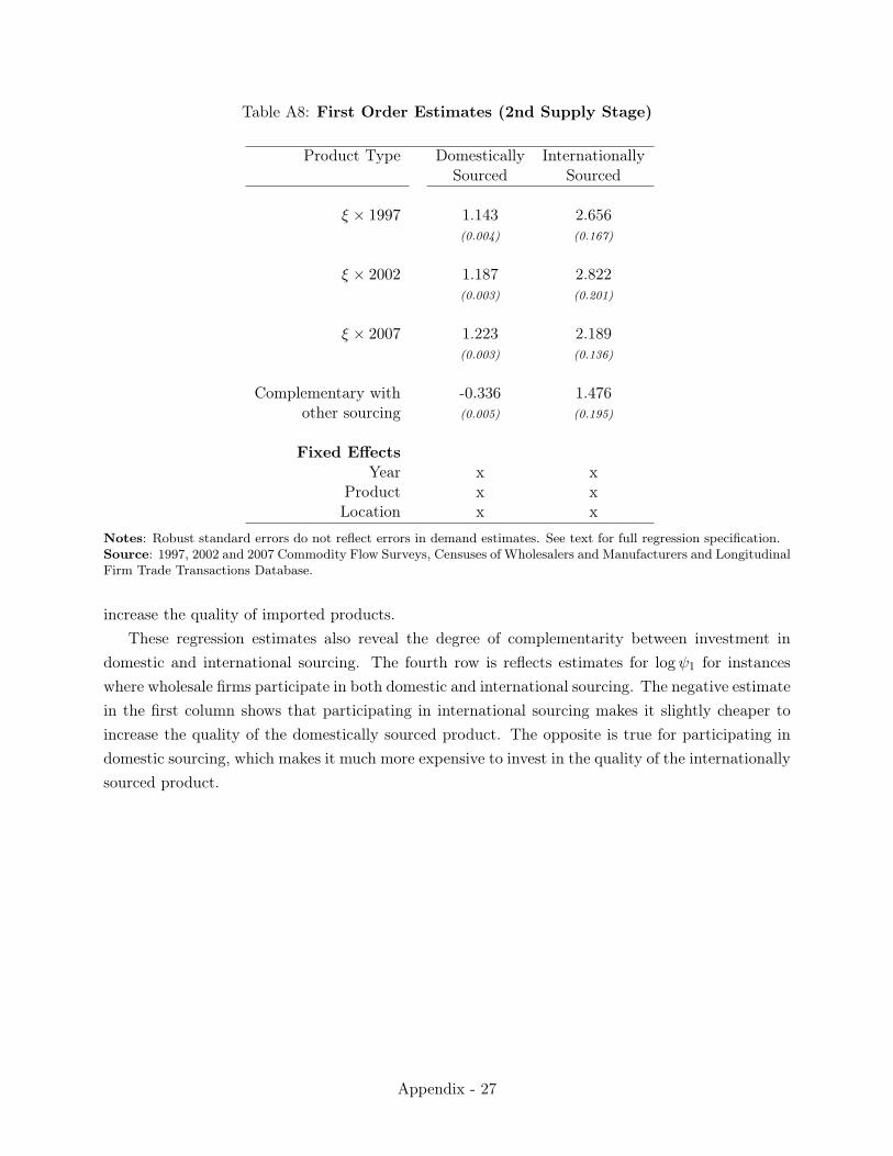
Table A8: First Order Estimates (2nd Supply Stage)

Product Type Domestically InternationallySourced Sourced

⇠ ⇥ 1997 1.143 2.656(0.004) (0.167)

⇠ ⇥ 2002 1.187 2.822(0.003) (0.201)

⇠ ⇥ 2007 1.223 2.189(0.003) (0.136)

Complementary with -0.336 1.476other sourcing (0.005) (0.195)

Fixed EffectsYear x x

Product x xLocation x x

Notes: Robust standard errors do not reflect errors in demand estimates. See text for full regression specification.Source: 1997, 2002 and 2007 Commodity Flow Surveys, Censuses of Wholesalers and Manufacturers and LongitudinalFirm Trade Transactions Database.

increase the quality of imported products.These regression estimates also reveal the degree of complementarity between investment in

domestic and international sourcing. The fourth row is reflects estimates for log 1 for instanceswhere wholesale firms participate in both domestic and international sourcing. The negative estimatein the first column shows that participating in international sourcing makes it slightly cheaper toincrease the quality of the domestically sourced product. The opposite is true for participating indomestic sourcing, which makes it much more expensive to invest in the quality of the internationallysourced product.

Appendix - 27