THE RENORMALIZATION GROUPAND THE ~EXPANSION

Kenneth G.WILSON

Institutefor AdvancedStudy,Princeton,N.J. 08540, USAandLaboratoryofNuclearStudies,Cornell University,Ithaca,N Y. 14850, USA

and

J.KOGUT

InstituteforAdvancedStudy,Princeton,NJ. 08540, USA

INORTH~HOLLANDPUBLISHING COMPANY — AMSTERDAM

PHYSICSREPORTS(SectionC of PhysicsLetters)12, No. 2 (1974) 75—200. NORTH-HOLLAND PUBLISHING COMPANY

THE RENORMALIZATION GROUP AND THE e EXPANSION*

KennethG. WILSONInstitutefor AdvancedStudy,Princeton,N.J. 08540, USA

and LaboratoryofNuclearStudies,Cornell University,Ithaca, N Y. 14850, USAt

and

J. KOGUT~Institutefor AdvancedStudy,Princeton,NJ. 08540, USA

Received2 July 1973

Abstract:

Themodernformulation of therenormalizationgroupis explainedfor both critical phenomenain classicalstatisticalmechanicsandquantumfield theory.Theexpansionin e = 4 — d is explained [d is thedimensionof space(statisticalmechanics)or space-time (quantumfield theory)1. Theemphasisis on principles, notparticularapplications.Sections1—8 providea self.containedintroductionata fairly elementarylevel to thestatisticalmechanicaltheory.No backgroundis requisedexceptfor somepriorexperiencewith diagrams.In particular,a diagrammaticapproximationto anexactrenormalizationgroupequationis presentedin sections4 and5; sections6—8 include theapproximater~normalizationgroup recursionformulaand theFeynmangraphmethodfor calculatingexponents.Sections10—13go deeperinto renormalizationgrouptheory (section9 presentsa calculationof anomalousdimensions).The equivalenceof quantumfield theory and classicalstatisticalmechanicsnearthecritical point isestablishedin section10; Sections11—13 concernproblemscommonto both subjects.Specific field theoreticreferencesassumesomebackgroundin quantumfield theory.An exactrenormalizationgroupequationis presentedin section11; sections12 and13 concernfundamentaltopologicalquestions.

Singleordersfor this issue

PHYSICSREPORTS(SectionC of PHYSICSLETTERS) 12,No. 2 (1974)75—200.

Copiesof thisissuemaybe obtainedat thepricegivenbelow.All ordersshouldbe sentdirectly to thePublisher.Ordersmustbe accompaniedby check.

SingleissuepriceDfl. 32.50,postageincluded.

*Basedon lecturesgivenatPrincetonUniversityby K.G.W.

tPresentaddressof bothauthors.~Worksupportedby theU.S. Atomic EnergyCommission,ContractNo. AT(1 1-1)2220.

K. G. WilsonandJ. Kogut, The renormalization group and thee expansion 77

Contents:

1. Introduction 78 7.2. Scalingtheoremsfor n-spin correlationfunctions 1281.1. Therenormalizationgroupandcoherence 7.3. Slow transientsandtheir removalfor smalle 132

problemsin physics 78 8. Feynmangraph calculationof critical exponents1.2. Currentreferences 83 (e expansion) 1331.3. Elementaryfactsabout theIsing model 86 9. Dimension of tensoroperatorsin 4—c dimensional

2. 87 space-time 1382.1. Elementarypropertiesof systemsneartheir 10. Connectionbetweenstatisticalmechanicsand

critical temperature 87 field theory 1432.2. Thesearchfor analyticity 90 11. Exact renormalizationgroupequationsin

2.2.1. Meanfield theory 90 differential form 1522.2.2. Kadanofftheory 92 12. 159

3. Trivial exampleof the renormalizationgroup: The 12.1. Topologyof the renormalizationgroupGaussianmodel 94 transformation(fixed points, trajectories,and

4. Thes4 model 101 subspaces) 159

4.1. Simplified renormalizationgrouptransformation106 12.2. Fixed points,subspaces,andrenormalization 1664.2. Thec-expansionanda non-trivial fixed point 107 12.3. Multiple fixed points,domains,and4.3. Linearizedequationsandcalculation.of r’ 107 universality 168

5. The~4 model (cont’d.) 111 12.4. Fixed pointsandanomalousdimensions 1725.1. Irrelevantvariablesandthee expansion 111 13. Futile (sofar) searchfor a non-trivial fixed5.2. Completerenormalizationgrouptransformation 116 point ~4 field theory in 4 dimensions 176

6. The approximaterecursionformula 117 14. Concludingremarks 1866.1. Polyakov’sderivation 117 Acknowledgements 1876.2. Somenumericalresults 120 Appendix: Simplesolutionsof theexact

7. 123 renormalizationgroupequations 1887.1. Moreresultsfrom theapproximaterecursion References 193

formula 123 Recentreferences 196

78 K. G. Wilson andJ. Kogut, The renormalizationgroupand thee expansion

1. Introduction

The purposeof this paperis to discussrecentwork on the renormalizationgroupand itsapplicationsto critical phenomenaand field theory.Theseideasareillustratedusing theotherrecentideaof definingcritical phenomenaand field theory in a spaceof dimension4—c (space-time dimension4—c for field theory)andexpandingin powersof e. The emphasisis on criticalphenomena;basicideaswill be stressedratherthanspecialresults.The presentationis incomplete;this reviewis not a substitutefor current literature.The first sectionis generalandphilosophical.Most of the subsequentsectionsaremorepragmatic,beingconcernedwith specificproblemsandcalculations.

Associatedwith this sectionthereis a list of recentreferenceson the renormalizationgroupand thec expansion.

For a preciselist of topicsdiscussedin this paper,seethe contents.

1. 1. The renormalizationgroup andcoherenceproblemsin physics

In this sectiona philosophicaldiscussionof the renormalizationgroupwill begiven. (Oneshouldrereadthisintroductionafter studyingtherestof the paper.)Toward the endof the firstsectionwe begin the reviewof critical phenomena.

The renormalizationgroupis a methodfor dealingwith someof themostdifficult problemsof physics.Theseproblemsincluderelativistic quantumfield theory,critical phenomena,theKondoeffect [e.g. l—7] and others.Theseproblemsareall characterizedby involving a largenumberof degreesof freedom,in an essentialway.

Most of theproblemsonedealswith in physicsinvolve a very largenumberof degreesoffreedom.For example,a crystal, liquid, or gasin macroscopicquantitiesinvolvesmore than1023electrons,andeachcoordinateof eachelectronis a degreeof freedom.

In contrast,most theoreticalmethodswork only whenonehasonly oneindependentvariable,i.e. only onedegreeof freedom.For example,considerthe Schrodingerequationfor a wavefunction i,Li (x, y,z) for one electron.It is infinitely easierto calculate~,1iif onecanseparatevariablesin the Schrodingerequation(e.g.,write ~Ji= ~Li1(r)Vi2~O)~4i3(~)in sphericalpolarcoordinates).It is obviouslyhopelessto computeawave function for 1023 electronswithoutextraordinarysimplifications,justified or otherwise.

Undernormal circumstancesthe 1023 or sodegreesof freedomcan be reducedenormously.The intensiveor extensivecharacterof observables(energyis extensive,densityis intensive)allowsone to reconstructthe propertiesof a macroscopicsystemgiven only a microscopicsampleof it. Thus a liquid of only 1000 atoms,say,would probablyhaveapproximatelythesameenergyper unit volumeanddensityas the sameliquid (at the sametemperatureand pressure)with 1023atoms.

How far canonereducethe size of a gas,say,without qualitatively changingits properties?The minimumsize onecanreachwithout changeis called the correlationlength.The correlationlength~ dependson the stateof the system.For agas~ dependson pressureand temperature.Infavorablecircumstances~ is only oneor two atomicspacings.When ~ is thissmall thereexist avariety of methodsfor calculatingpropertiesof thesystem:virial expansions,perturbationexpansions,Hartree-Fockmethods,etc.Thesemethodsinvolve a variety of approximations;buttheyhaveone featurein common.They all assumethat the propertiesof matterin bulk canberelatedto the propertiesof smallclustersof atoms.They involve furtherassumptionsbecauseevena clusterof only threeatomsinvolvestoo many degreesof freedomto be solublewithoutconsiderablesimplification.

K. G. WilsonandJ. Kogut, The renormalizationgroup and the e expansion 79

In specialcasesthe correlationlengthis much largerthanthe atomicspacing.The critical pointmarkingthe onsetof a phasetransition is a prime example.Liquid-gastransitions,ferromagnetictransitions,order-disordertransitionsin alloys, etc.,all exhibit critical points for specialvaluesofthe thermodynamicvariables.(The liquid-gascritical point occursfor critical valuesT~and~c oftemperatureandpressure.)Preciselyat the critical point, ~ is infinite; nearthe critical point ~ islarge.

Therearea classof problems,including critical phenomena,which arecharacterizedby havingvery manydegreesof freedomin a region the size of acorrelationlength. “Very many” meansnot just 3 or 4, but hundredsor millions if not an infinite number.Otherproblemsof this typebesidescritical phenomenaarethe Kondoproblem(a magneticimpurity in a metal), the bindingof largemolecules,andthe entiresubjectof relativistic quantumfield theory. In the caseof aquantumfield, say ~(x), the field ~ at eachpoint x is a separatedegreeof freedom,soany regionof finite size containsan infinite numberof degreesof freedom.The correlationlengthof aquantumfield is usuallythe Comptonwavelengthof the lowestmassparticle. In the caseofquantumelectrodynamicsit is the electronComptonwavelength(10’’ cm) rather than thephotonComptonwavelength(oo) which actsas the correlationlengthin practice.Onecanrelatively easilyrelatequantumelectrodynamicsin a box of size >10-11 cm to quantumelectro-dynamicsin all space.Boxesof size ~ 10h1 cm causegrossdistortionsof the interactionsofelectronsandphotons.

The problemslistedaboveareall notedfor their intransigence.The binding of moleculesishardly betterunderstoodtodaythanit was in 1932.Therehasbeenfitful progressin criticalphenomenaover thelast 70 years.Therehasbeensensationalprogressin calculatingquantumelectrodynamics,but very little progressin understandingit; andstronginteractionsareneithercalculablenorunderstood.The Kondoproblemhasonly recentlybeenstudied,andmaybe closerto solution [2,3,7].

Studiesof renormalizationin quantumfield theoryandcritical phenomenain statisticalmechanicsboth suggestthat the behaviorof systemswith manydegreesof freedomwithin acorrelationlengthis qualitativelydifferent from thosewith only a few degreesof freedomin acorrelationlength.The systemswe areinterestedin areusuallydefinedby meansof aHamiltonian,andonewould normallyhaveexpectedthat thebehaviorof the systemis deter-minedmainly by the typeof interactionspresentin the Hamiltonianandthe strengthsof thecorrespondingcouplingconstants.This is certainlythe casewhen~ is small. However,in theproblemsdiscussedhere,wheremanydegreesof freedomarebehavingcooperatively,it appearsthat the behaviorof the systemis determinedprimarily by the fact that thereis cooperativebehavior,plus the natureof the degreesof freedomthemselves.The interactionHamiltonianplaysonly a secondaryrole. Thus,in critical phenomenatherehasdevelopedthe notion ofuniversality,i.e. that all interactionHamiltoniansshowthe samecritical behavior.The ideaofuniversalityoriginatesin the “law of correspondingstates”,which is thehypothesisthat all fluidsandgaseshavethe sameequationof stateapartfrom a renormalizationof length andenergyscales.For a comparativelyrecentreferenceon this law seeGuggenheim[8]. Recentlythe ideaofuniversalityhasbeenformulatedmoregenerallyto relatecritical behaviorin differentsystemswith arbitraryinteractions.Seefor exampleKadanoff[9]. Universalitywill be discussedfurtherbelowandin section 12.

The renormalizationgroupapproachhastwo objectives.The first is the practicaloneofsimplifying the taskof solving systemswith manydegreesof freedomcontainedwithin a correla-tion length.The basicideais thesameas in hydrodynamics.In hydrodynamicsoneintroducesnew variablessuchas the densityp(x) which representsanaverageover the original microscopicdegreesof freedom.All microscopicfluctuationsareeliminatedin the hydrodynamicequations;

80 K. G. Wilsonand.1. Kogut, The renormalizationgroup and the e expansion

p(x) is supposedto showonly macroscopicfluctuations.Whatthis meansin effect is that thehydrodynamicdegreesof freedomarethe valuesof p(x) at macroscopicallyseparatedpoints.Thus,therearefar fewer hydrodynamicdegreesof freedomperunit volume thanoriginal micro-scopicdegreesof freedomper unit volume.

The renormalizationgroupapproachis similar to the hydrodynamicapproachin that againtheoriginalmicroscopicdegreesof freedomarereplacedby a smallersetof effectivedegreesoffreedom.This is donein steps;in eachstepthe linear densityof degreesof freedomis reducedbya factor 2.

Reducingthe “densityof degreesof freedom” canbe realizedin severalways. Supposetheoriginal systemwas a systemof spinswith spacingL0. The new effectivedegreesof freedommightbe spinswith spacing2L0. Alternatively the new degreesof freedommight be a magnetizationdensityM(x) dependingon a continuousvariablex (just as hydrodynamicsreplacesdiscreteatomsby a densityp(x)). Then to limit the degreesof freedomoneimposesthe restrictionthatM(x)only containsfluctuationswith wavelengthsgreaterthan2L0. Theseideaswill be formulatedmorepreciselyin later sectionsof this review. (Thefactorof 2 is arbitrary. In particular,it isoftenusefulto changethe densityof degreesof freedomonly infinitesimally insteadof by afactor 2. Seelatersections.)

Thisreductionin the degreesof freedomis carriedout repeatedly.To startwith, the spacingof degreesof freedomis L0 after 1 stepthe spacingis 2L0, after2 stepsthe spacingis 4L0, etc.Oneproceedswith furtherstepsuntil theseparationof effectivedegreesof freedomis of orderthe correlationlengthE. In eachsteponehasto constructan effectiveinteractionfor the effectivedegreesof freedom,just asin hydrodynamicsonehasto constructthehydrodynamicequationsfor p(x). The simplification of the renormalizationgroup lies in the hopethat theseeffectiveinteractions~ ~IC2,etc. are local interactions,i.e. the interactionsshould coupledirectly onlynearbydegreesof freedom.Thisof courseassumesthatthe initial interactionwas local, but thisis true for the problemsof interesthere.Thuswe assumethat therangeof interactionin theinitial interactionis of orderL0 evenwhen~ ~ L0. The hopeis that therangeof interactionin~fC1is of order2L0, the rangeof interactionin ~JC2is of order4L0, etc.The alternativeis that therangeof interaction is ~ evenfor ~C1,which would be disastrousfor therenormalizationgroupapproach.This disasteris avoidedin the examplesthathavebeenworkedout so far, but maybe aproblemin othercases.

If it is true that the rangeof interactionin ~ is only of order2L0, thenonecanimagine(againby analogyto hydrodynamics)thatthe couplingconstantsin ~IC1canbe determinedbystudyingthe behaviourof the systemconfinedto a regionof size (of order)2L0 i.e. onedoesnot haveto discussregionsof size ~. Thusoneno longerhasa hugenumberof degreesof freedomto worry about.To determinethe couplingconstantsin ~JC2requiresa largerregionof size 4L0.However, the ideahereis to determine~iC2startingfrom ~C1whosedegreesof freedomarespacedby 2L0, insteadof the original interaction~IC0with spacingL0. Thenonestill hasa limitednumberof degreesof freedomto consider.In the sameway oneconstructs~JC3from ~C2,~W4from~JC3,etc., until oneobtainsthe ~fCnfor which 2°L0 ~. At this stageonehasonly a few degreesoffreedomper correlationlengthandthe problemcanhopefully be solvedby othermethods.Ingeneral,whencalculating~C1onehasto consideraregion of size 2’L0, but onestartsfrom ~C11

whosedegreesof freedomhavespacing21-1L

0 Thus for anyI onecanconsidera region contain-ing only a few effectivedegreesof freedom.

Unfortunately,the generalrenormalizationgrouptechniquesdo not reducethe problemto1 degreeof freedom.Onecaneasilyimaginethatoneneedsto consider60 or moreeffectivedegreesof freedomwhendetermining~C1from ~C1...~. Supposefor examplethat the effectivedegreesof freedomin 1C1 arediscretespins,andthatonehasto discussa three-dimensional

K. G. Wilson andJ. Kogut, The renormalizationgroup and the c expansion 81

cubeof width 4 spins: this cubewill contain64 spins.This is not very practical.Onemustsimplify the calculationfurtherso that ~ canbe computedfrom ~C11usingonly onedegreeoffreedom.The practicalapplicationsof therenormalizationgroupdescribedin laterlecturesinvolve eitherspecialcircumstances(the cased 4 — e with smalle) or crudeapproximations(the “approximaterecursionformula”) suchthatonly onedegreeof freedomis neededfor thecalculationof ~C1.(See,however,the supplementallist of references.)

The secondaim of therenormalizationgroup approachis to explainhow thequalitative featuresof cooperativebehaviorarise. In the renormalizationgroupframework, thesequalitativefeaturesresultfrom theiterative characterof the renormalizationgroup.Namely,thereis a transformationr whichconverts~C0to X1, ~1C1to ~C2,etc. The transformationis the samewhetheroneis con-structing~IC1from ~C0or ~IC2from ~JC1in eachcaseoneis thinning the degreesof freedomby afactor 2. The only differenceis in the lengthscale(L0 versus2L0) which is easilytransformedaway.Soonehasa transformationr which is to be appliedrepeatedly:

r(~C0)= ~lC1, r(~JC1) ~C2, r(~JC2)= ~1C3 etc. (1.1)

This transformationis to be iteratedn timeswhere2°L0is of order ~. When ~ is large,thenumberof iterationsis large.

Whenonehasa transformationr which is iteratedmany times,the simplestresultwe canobtainis that the sequence~tC1approachesa fixed point of r, namelyan interaction~lC*satisfying

r(~C*)= ~ (1.2)This is what will happenin the examplesdiscussedlaterin this review.

A fixed point of a transformationis a propertyof the transformationr itself. That is, to findpossiblefixed point Hamiltonians~1C~onemustsolve the fixed point equation(1.2). Theseequationsmakeno referenceto the choiceof initial Hamiltonian~1C0.

The possibletypesof cooperativebehavior,in the renormalizationgrouppicture, aredeter-minedby the possiblefixed points~C*of r. Supposefor examplethat thereare threefixed points1C~,~ and~ Thenonewould havethreepossibleforms of cooperativebehavior.If a particu-lar systemhasan initial interaction~IC0,onehasto constructthesequenceX1, ~C~’etc. in order tofind out which of ~CZ,~ or ~JC~gives the limit of the sequence.If ~CZis the limit of thesequence,thenthe cooperativebehaviorresultingfrom ~lC0will be the cooperativebehaviordeterminedby ~ In this examplethesetof all possibleinitial interactions~JC0woulddivide intothreesubsets(called“domains”), onefor eachfixed point. Universalitywould now hold separatelyfor eachdomain.Seesection 12 for furtherdiscussion.

This is how onederivesa form of universalityin the renormalizationgrouppicture. It is not sobold as previousformulations [91.Experiencewith solubleexamplesof the renormalizationgrouptransformationfor critical phenomenashowsthat it generallyhasa numberof fixed points,soonehasto definedomainsof initial Hamiltoniansassociatedwith eachfixed point, andonly within agiven domainis the critical behaviorindependentof the initial interaction.

Thereis no apriori requirementthat the sequence~JC1approacha fixed point for 1 -+ ~ Inprinciple the sequencefor large1 could show limit cycle,ergodicor turbulentbehavior;in such.casesit would be difficult to do much calculation.See[10] for an illustrationof ergodicandturbulentbehavior. But evenif the sequence~C1doesnot approacha fixed point, it is unlikelythat ~1C~for largen is a smoothfunctionof the parametersin X0. The trouble is that smallchangesin the parametersin ~1C0tendto be amplified ordeamplifiedby the transformationr, andwhenris iteratedmanytimestheseamplificationor deamplificationfactorsbecomevery large(onewould guessof order~/fffrom randomwalk arguments).Thus if u0 is a couplingconstantin JC0onewould expectlargerangesof u0 which aredeamplified(~JC~dependsvery little on u0)

82 K G. Wilson and J. Kogut, The renormalizationgroup and the � expansion

separatedby smallrangesof u0 which areamplified (~Cnchangesvery rapidly with u0). In the casethat all sequencesapproachfixed points,the rangesof u0 for which amplificationoccursarethosevaluesof u0 for which ~C0is nearthe boundarybetweentwo domains,while deamplificationoccurswhen~1C~is well insidea particulardomain.

In summary,the basicideasof the renormalizationgroupare,first, to generatea sequenceofeffectivelocal interactions~JC1.That is, if the spacingof degreesof freedomin ~JC1is a~thentheinteractionsshouldhaverangea1 not ~ andby choosinga1÷1 2al oneshouldbe ableto construct~fC1+1from ~fC1consideringregionsof size about~ rather than~. Secondly,the existenceof atransformationr which is iteratedrepeatedlyto construct~1C1from ~JC0suggeststhat the natureof~C1for large1 will be largelyor wholly determinedby r itself ratherthanXç,, therebyleadingto atleasta limited form of universality.

To concludethis introductionwe outline briefly the history of therenormalizationgroupmethod.This discussionis not completeandprobablynot very accurate.Landau[11] proposeda hydrodynamicapproachto critical phenomenain the late 1930’s. His specifictheorygavethesameresultsas earliermeanfield theory,which is experimentallyfalse.However, therenormaliza-tion groupapproachis bestseenas a moresophisticatedrealizationof Landau’sideas.

The specific ideasof the renormalizationgroup approachappearedin two papersof theearly1950’s,in connectionwith quantumfield theory.A formulationof the renormalizationgrouptransformationr was given by StueckelbergandPetermann[121. Gell-MannandLow [13], in aremarkablepaper,discussedthe ideaof afixed point of the transformationandsomeof itsimplications: theyshowedthat auniquevalue of thebarechargee0 in quantumelectrodynamicswould correspondto all (sufficiently small) valuesof the renormalizedchargee. This is theamplificationeffectdiscussedearlier. In the limit of infinite cutoff (i.e. in the limit of infinitesimalspacingof the original degreesof freedom)r is iteratedaninfinite numberof times. Thusonecaninfinite amplification,e.g. a continuousrangeof valuesof e correspondingto onevalueof e0. Therecipesfor renormalizationgroupcalculationswerereviewedin BogoliubovandShirkov [14].

The earlywork on the renormalizationgrouphad two defects.It had no calculableexperimentalconsequences,sono onehadto takeit seriously.Secondly,the intuitive ideaswereencasedin athick shell of formalism; it hasrequiredmanyyearsto peel off theshell.

In the 1960’san extraordinarypaperby Kadanoff [15] on critical phenomenacontainedanintuitive discussionof theideaof thinning the degreesof freedom.Kadanoffassumedthatonecoulddiscussblocksof spinsin a ferromagnetas if theywere singleeffectivespinswith verysimple interactions.Kadanoffshowedthat this assumptionimplied asetof “scalinglaws” relatingcritical exponentswhich hadbeenpostulatedearlierby Widom andothers(see [161 forreferences).Kadanoffdid not haveashredofjustification for his assumption;the importanceofhis work was that it provideda simplebut idealpictureof what an effectivedegreeof freedomwould be andhow it would interact.This pictureis surelyunrealizablein practice.Whatonedoesis try to comeas closeas onecan to this picture.Onetriesto defineeffectivedegreesoffreedomwhich areroughly describableas block spins,andinteractionswhich havea simpleform(not necessarilyIsing-like), at leastapproximately.In summary,Kadanoffhasdefineda muchmoreprofitablegoal to work towardsthanthe elaborateformalismsof the earlierwork.

The differentialequationsof the renormalizationgroupresurfacedin the Kondoproblemin thework of Andersonetal. andothers[2—7]. Anderson[4] was the first to derivetheseequationsexplicitly usingtheidea of reducingthenumberof degreesof freedom.The previousfield theoreticwork hada muchlesstransparentjustification.

Until recently all formulationsof the renormalizationgroupinvolved a transformationr actingon a very restrictedspaceof interactions.Gell-Mann andLow consideredthe standardelectro-dynamicinteractionwith the chargee0 as the only free parameter.Kadanoffallowedonly

K. G. WilsonandJ. Kogut, The renormalization groupand the � expansion 83

nearestneighborIsing-typeinteractions.A heavypriceis paidfor this restriction:onecanonlydefiner when thesolution of theproblemis known.For example,Gell-Mann andLow definerin termsof the exactelectronpropagator,which is not knownuntil electrodynamicsis solved.Thus thereis only alimited possibility of usingthe renormalizationgroupto helpin solving thetheory.A studyof the fixed sourcemodelof the nucleon,in simplified form, showedthat thisproblemdisappearsif oneis willing to let ~IC1containall possibleinteractions,not just oneor two[17]. It is thenrelatively easyto constructexamplesof the transformationr without solving thetheory (seelaterlectures).Now onepaysa differentprice: onecannotkeeptrackof all possibleinteractionsat oncebecausetherearetoo manyof them.So onehasto haveonly a few dominantinteractionsif therenormalizationgroupapproachis to be practical.Therecanbe manymoreinteractionswith smallcouplingconstants,as long as thesecanbehandledby perturbationmethods.This was preciselythesituationin the fixed sourcemodel. It is alsotrue in the examplesdiscussedlater in this review,but it is not at all certainto be true in general.

Currentwork on the renormalizationgroupwill be summarizedbelow.Therehavebeenotherideasfor dealingwith problemssuchas critical phenomena.We mention

specificallythe Migdal-Polyakovbootstrapapproachto critical phenomenaand field theory[18—26] andthe Johnson-Baker-Willeyformulationof electrodynamics[27—29] becausetheseideasaresometimesconfusedwith the renormalizationgroupapproach.Thereis no transformationlike r in either the Migdal-Polyakovor Johnson-Baker-Willeytheories;theseauthorsmakenoattemptto thin the degreesof freedom.So their ideascannotbe classifiedasrenormalizationgroup methods.In placeof consciouslyreducingthenumberof degreesof freedom,theseauthorssubstitutea prayerthat an infinite sumof graphscanbe replacedby acalculablesubset.Seebelowfor furthercomments.

Anotherrecentdevelopmentis the Callan-Symanzikequations[30, 31]. Closelyrelatedto theoriginal Gell-Mann---Low formulationof the renormalizationgroup, theseequationsareproving tobe valuabletools for analyzingtheshortdistancebehaviorof Feynmangraphs[e.g.321. Atpresentthe Callan-Symanzikequationsaretoo formal to be practicaloutsideof perturbationtheory.They will remainsounlesssomeintuition canbe addedthe way Kadanoffaddedanintuitive pictureto the renormalizationgroup approach.

1.2. Currentreferences

Currentliteratureon the renormalizationgroupwill now be classified,briefly. Seealsothesupplementallist at the endof this review. First, paperson critical phenomenawill be listed.Theapproximaterenormalizationgroup recursionformulais derivedin [33]. Numericalsolutionsof the recursionformulafor the Ising casearein [33]. Grover,Kadanoff,andWegnersolvedtheHeisenbergcasenumerically [34]. Grover solvedtheX—Ymodelnumerically [35]. Baker[36]and Dyson [37] havedescribed“hierarchical”modelsfor which the recursionformulais exact.Golner[381 hasproposeda form of the recursionformulawhich givesa non-zerovalueof~(i~is definedin section2). Golner [39] hassolvedthe recursionformulafor anexamplewith three-fold symmetry.The e expansionabout4 dimensionswas developedby FisherandWilson [40].A calculationof the scalingpropertiesof all perturbationsaboutthe critical point, within thee expansion,is given by Wegner[41] ; Fisherand Pfeuty [42] investigateslightly anisotropicHeisenbergmodels.The recursionformulahasbeenappliedto tricritical points(suchas3He—4Hemixtures)by RiedelandWegner[43]. The methodsof ref. [331 havebeenappliedtothe problemof phaseseparationby LangerandBar-on [44].

The Feynmangraph methodfor calculatingcritical exponentsin powersof c (section8) wasdevelopedin [45]. It was appliedto the “excludedvolume” problemby De Gennes[46].

84 K. G. WilsonandJ. Kogut, Therenormalization group and the � expansion

Nickel [47] hascalculatedthe exponent‘y to ordere3. The � expansionfor theequationof statenearthe critical point hasbeenobtainedby Brézin, WallaceandWilson [48], [49]. The chargedandneutralBosegasis discussedby Ma [50]. Exponentsin the presenceof long rangeforcesarecomputedby Suzuki [51, 52] andFisher,Ma, andNickel [531.

The Gell-Manri—Low formulationof the renormalizationgroupwas usedby Larkin andKhmel’nitskii [54] to discussthe logarithmic behaviorof critical phenomenain four dimensions(e = 0) anduniaxial ferroelectricsin threedimensions.DePasquale,Di CastroandJona-Lasinio[55—57] andMigdal [58] havediscussedqualitativeimplicationsfor critical phenomenaof theGell-Mann—Lowformulation.Di Castro[59] hasusedthe Gell-Mann--Lowtheory to confirmsomeresultsof [45]. Wegner[601 hasgiven an extensivediscussionof all kindsof perturbationsaboutthe critical point with emphasison correctionsto the scalinglaws,usingthe modernformulation(seealsosection 12). Severalquestionshavebeendiscussedby Hubbard[61]; theproblemof liquids is discussedby HubbardandSchofield [62]. The Gaussianmodelwith longrangeforcesis discussedby NiemeijerandVan Leeuwen[63].

The work of Dyson [37], Larkin andKhmel’nitskii [54] andDi CastroandJona-Lasinio[55—57] precededthework describedin this report. For a good surveyof critical phenomenajust prior to the new developments,seethe entirevolumeof ref. [56]. The new work issummarizedbriefly in [64].

Many of the referenceslistedabovereport specificapplicationsof the renormalizationgroupapproachwhich are omittedfrom this review.

Thereis another(earlier, but incomplete)paper(setof lecturenotes)on the renormalizationgroup [651. They concerntheideasof the modernrenormalizationgroupapproachwith lessemphasison calculationthanthe presentreport.

The closemathematicalanalogybetweencritical phenomenaand quantumfield theory hasbeenemphasizedby Gribov and Migdal [66, 67] andPolyakov [68—70] in termsof Feynrnandiagrams;Moore [71] comparesthe Feynmanpathintegralto the partition function;Suri [72]makes the connection using the transfermatrix formalism of statisticalmechanics(seesection 1 U).

For areview of work on the renormalizationgroupin quantumfield theoryusingtheGefl-Mann—Low formulation see [73]. For a field theoreticformulationof the approximaterecursionformula,see [74]. SeelikewiseGolner [751.

The ideaof a nonintegerdimensiond andan expansionaboutd = 4 is a usefultheoreticaldevicewithoutphysicalsignificance:the physicsis only in integerdimensiond. Nonintegraldimensionswill be introducedby analyticcontinuationin renormalizationgroupequations(section4) orFeynmangraphs(section8). The ideaof nonintegraldimensionsin statisticalmechanicsis notnew: see [761 for example.More recently,Widom hasstudied 1 + e dimensions[77]. Nonintegerd hasbeenusedrecentlyin field theoryto regularizeFeynmangraphs [78—80]; a thoroughdiscussionis given in ‘t Hooft andVeltman [781. Quantumfield theoryfor nonintegerd isdiscussedin [81] wheretheeexpansionis usedto computeanomalousdimensions(seealsosection9).

Anotherexpansiontechniquein bothcritical phenomenaandfield theory is the 1/N expansionwhereN is thenumbero~finternal componentsof a spin (critical phenomena)or the numberofinternalcomponentsof a quantumfield. Stanley [82] discoveredthat thelimitN—* oo for a spinsystemreducesto the solublesphericalmodelof Berlin andKac [831. This was discussedfurtherby Kac andThomson[84]. Techniquesfor expandingexponentsin 1/N werediscoveredby Abe[85] andWilson [81]. They havebeenexploitedby Abe andHikami [861, [871, Suzuki [51],[521, Ma [50], [88], Fisheret al. [531,and Ferrell andScalapino[891. Brézin andWallace [901andSuzuki[52] havecomputedtheequationof stateusingthis expansion.The expansionis

K. G. Wilson andJ. Kogut, The renormalizationgroup and the � expansion 85

probablynot very usefulfor N 1 to 3, the casesof mostphysical interest.This is becausethe �expansion(valid for anyN) hasdenominatorsof the form N + 8 (seesection8) suggestingthe1/N expansionis valid only forN> 8. Howeverit is instructiveto studymodelswith largeN asmodelsin their own right. The applicationof the 1/N expansionto field theoriesin lessthanfourspace-timedimensionis discussedin [811.

Thereis aspecialsituationwheretheproblemof a largenumberof degreesof freedomwithina correlationlengthis trivial, namely free field theories(quantumfield theory)or the Gaussianmodelin statisticalmechanics(seesection3). Thesetheoriesaretrivial becausethe interactioncanbe diagonalizedin momentumspace.Thereexista variety of graphicalmethodsfor treatingsmallperturbationsabout thesetrivial theories.The � expansionmakesit possibleto do successfulcalculationsin critical phenomenaby perturbationmethods.Therearenow a bewilderingvarietyof methodsfor settingup the � expansion:besidesthe methodsdiscussedin this paper,De Castro[59] hasusedthe old Gell-Mann—Low methodsandMack [26] hasusedthe Migdal—Polyakovapproach.The new renormalizationgroupmethodis emphasizedin this paperbecauseof itspotentialfor handlingnonperturbativeproblems(seerefs. [33, 60] andsections12 and 13). Bycomparison,for problemswhich cannotbe reducedto a few diagrams,it is hopelessto calculateanythingusingthe Gell-Mann—Low theory.Evenfor questionsof principle the Gell-Mann—Lowtheory is not satisfactorybecauseit involvesassumptionswhich aretechnicalandnot physicallymotivated [73]. It is hard to believetheseassumptionsarealwaysvalid, althoughtheyappeartobe true orderby orderin a diagrammaticexpansion[e.g.73]. The Migdal—Polyakovbootstrap(with conformalinvarianceassumed)is moreinterestingalthoughnot very practicalunlessonly afew diagramsareimportant.For field theoristsan interestinganduniquefeatureof the Migdal—Polyakovbootstrapis Polyakov’s “streamunitarity” [91].

The nextsevensectionsareconcernedwith critical phenomena.This is partly becausethis isthe mostsuccessfulapplicationof therenormalizationgroupapproach.However,criticalphenomenaprovidesthesimplestandclearestexampleof the problemof manydegreesoffreedomwithin a correlationlength.The experimentsarepreciseand relatively unambiguousandtest the fundamentalaspectsof the theory.The simplestmodelslike the Ising modelhavenocomplicationsotherthanthebasicproblemof the largecorrelationlength.Thestudyof criticalphenomenagives onean overviewof the problemof manydegreesof freedomwithin a correlationlengththat cannotbe obtainedanyotherway andis essentialto understandthe field theoreticalapplicationsdiscussedin sections9—13.

Thereareexcellentreviewsof experimentandprevioustheoryof critical phenomena(seesection2); this reportwill be devotedto explainingthe renormalizationgroupapproach.Enoughbackgroundwill be suppliedsoonecan readthis reviewwithout previousbackgroundin criticalphenomena,but the relationof the renormalizationgroupto experimentandprior theorywillnot be discussedin detail.

Sections11, 12, and 13 areof importanceto statisticalmechanics;but the main interestfromsection9 on is quantumfield theory.Theydependheavily on the previoussections.Theyarepartof a seriesof papers[92, 73] explainingthe renormalizationgroup approachas an alternativetocanonicalfield theory.The ultimateaim is to producea field theoryof stronginteractions,butbreakthroughsarestill requiredbothin fundamentaltheoryandtechniquesof calculationbeforethe aim canbe realized.Meanwhile,thestudyof therenormalizationgroupapproachhaspro-vided, as a byproduct,usefulideaswhich havebeenincorporatedinto morephenomenologicalapproachesto stronginteractions[92, 93]. Particlephysicistswho havestudiedthe ideasof thispaperfind that it takesconsiderableeffort overa period of time to understandthem; theyprovidea stimulatingpoint of view on the problemsof quantumfield theory;andtheoutlookfor the future of theseideasis at presentuncertain.Seesection 14.

86 K. G. WilsonandJ. Kogut, The renormalizationgroup and thee expansion

1.3. Elementaryfactsabout the Ising model

Let us beginby discussingthe elementaryfeaturesof the Ising model. (For the history of theIsing model,see [94].) The modelhasservedin thepastasa descriptionof ferromagnetismbutprobablyalsoconstitutesa modelof relativistic field theory.We imaginea cubic latticeof points,n = (n1, n2, n3) in threedimensions,say, andattachto eachlatticepoint a spin variables,~.Wesupposethats,~takeson only thediscretevalues±1, so that it is not treatedas a full-fledged3-dimensionalquantummechanicalspin variable. If the latticeconsistsof N sites, the systemclearlypossesses2N possiblestates.Eachof thesespin configurationswill havea particularenergy.If only nearestneighborspin-spininteractionsareallowedthe Hamiltonianis,

H=—J>~~ s~s~+~ (1.3)

where{i} are theunit vectorsfor eachaxison thelattice (fig. 1. 1). Furthermore,if thelattice is

• • • S S

• S S S S

Fig. 1.1. A two-dimensionallattice,with unit vectorsfor eachaxis.

emersedin an externalmagneticfield B, the Hamiltonianacquiresanadditionalterm,

H—J~~snsn+i+pB>~sn (1.4)

wherep is a certaingyromagneticratio.The thermodynamicsof the systemcanbe obtainedfrom

the partition function

~ e”/’~~” (1.5){corfigurations }

wherethe sumrunsover all possiblespin configurationsof thelattice, T is the temperature,andkis Boltzmann’sconstant.It is alsoconvenientto introducea free energyF,

F—kTlnZ. (1.6)

Consideralsothe magnetizationper latticesite,

M — 1 ‘~‘ (ps~exp(—H/kT)> (1N ~‘ (exp(—H/kT))

where(. . .) standsfor a sumover configurations.M can be written

(1.8)

K. G. Wilsonand J. Kogut, The renormalizationgroup and thee expansion 87

The Ising model, in 2 or moredimensions,candisplayspontaneousmagnetization.Let thelatticebe in an externalmagneticfield B. If M remainsdifferent from zerowhenthe externalfield is removed,thereis spontaneousmagnetization.For example,this occursif at zero tempera-ture the stateof lowest energyof the systemhasall the spinsaligned.We canexpectM = 1 atzerotemperaturebut M = 0 at infinite temperature,wherethermalenergyoverwhelmsthe spin-spininteraction.Only for temperaturesT lessthana critical value Tc doesspontaneousmagnetizationoccur. Spontaneousmagnetizationis alsoclosely relatedto the behaviorof the spin-spincorrela-tion function definedby,

= (s,~s0exp(—H/kT)> (1.9)(exp(—H/kT))

At zerotemperaturewhenall the spins line up F,~is unity, independentof,i. However, asT-÷no

thermalexcitationswashout the spin-spincorrelations,soF~is different from zeroonly at theorigin. We will in fact seethat theway F,~falls to zeroasn increaseswill dependon whetherT < Tc, T = Tc or T> T~.The Ising model,therefore,containstwo lengths:the latticespacing,andthe distanceoverwhich spin-spincorrelationsareappreciable.

2.

In the first sectionwe discussedthe Ising modelandthe phenomenologyof a critical point,suchas the critical temperatureat which spontaneousmagnetizationfirst occurs.We will studythroughsevensectionstheproblemof critical behaviorlooking specificallyat phenomenaabovethe critical temperaturewhere,althoughthereis no spontaneousmagnetization,the systemfeelsthe presenceof the nearbycritical point. In this sectionwe will considervarioustheoriesof thecritical point atthe handwavinglevel: Landau’sform of meanfield theory,andtheKadanofftheoryof effectiveinteractionsinvolving block spins.This secondapproachwill provide thebackgroundfor the renormalizationgroup.(Somestandardreferenceson critical phenomenaarerefs. [95—lOll.)

2.1. Elementarypropertiesofsystemsnear their critical temperature

If we plot the spontaneousmagnetizationversustemperaturefor a ferromagnet,an anti-ferromagnetor the Ising model,onefinds a curvesimilar to that shownin fig. 2.1. Thereis acritical temperature,T~,at which spontaneousmagnetizationfirst occurs.The curverisesto somefinite valueat temperaturezero. In the regionjust belowthe critical temperature,themagnetiza-tion is well approximatedby a powerlaw,

M0(Tc_TY~ (2.1)

where~ is an exampleof a critical exponent.Theoriesof critical behavioraremainlyconcernedwith predictingsuchcritical exponentsor, atleast,finding relationsbetweenthem.

Thereis alsothe correlationlengthwhich we introducedearlier.Considertwo spins,oneatlatticesite n, oneat the origin anddefinethe correlationfunction,

= (s~s0exp(—H/kT))/(exp(—H/kT)) (2.2)

where(. . .) indicatesa sumover all configurations.The correlationfunctionhastheproperty

88 K. G. Wilson andJ. Kogut, The renormalizationgroupand the � expansion

~xp~-lflj/E(Tl

)

I I I I I I I I 1 0

Fig. 2,1. A graph of magnetization Fig. 2.2. Spin-spincorrelationversustemperaturefor a ferromagnet. function versusdistancebetweenTc is the critical temperature, sites. Curve(1) is anexamplewith

T> Tc; curve(2) is anexamplewith T< Tc.

thatif T> Tc, thenF,~fallsoff with ni (curve 1 in fig. 2.2). The asymptoticbehaviorfor large

ni is thoughtto be’

F,~‘~-‘exp{—Ini/~(T)} (2.3)

whereE(T) is the correlationlength.(Thereare variouswaysof definingthe correlationlength.It is not evidentthat thequalitativedefinition of section1 (see,in particular,the discussionp. 78)agreeswith the precisedefinition of (2.3). They will in fact not alwaysagree,but for the IsingmodelaboveTc they do agreeso far as is known.)Unfortunately,due to the complexityof thesystem,the validity of (2.3) hasnot beenprovedin general.For T < Tc, the correlationfunctionis expectedto approachthe squareof the magnetizationdividedby thesquareof the magneticmomentas n increases(curve 2, fig. 2.2). In otherwords, for largen actualcorrelationhasdisappearedandwhat remainsis theproductof the expectationvaluesof the singlespins.At thecritical temperaturethe correlationfunction falls to zerofor largen becausethereis no spontan-eousmagnetization.However,it fallsvery slowly (fig. 2.3)becausewe areat a transitionpoint.The correlationfunctionat T~is expectedto fall as a powerof n and,by convention,is writtenin the form

ç1/1~1d_2+~ (2.4)

whered is thedimensionalityof the system.In two dimensionswe know that (2.4) is the correctform of the correlationfunction [95]. However,in threedimensionsthe statementis just a guess.~ definesa secondcritical exponent.

- n

Fig. 2.3. Correlationfunctionat thecritical temperature. Fig. 2.4. Correlationlengthplotted

againsttemperature.

Onecanalso considerthe correlationlength~(T) itself. ~(T) setsthescalefor the falloff of thecorrelationfunctionwhen T is aboveTc. As shownin fig. 2.4, ~(T) approachesinfinity as T-~’T~from above:

(2.5)

K. G. Wilsonand J. Kogut, The renormalizationgroup and the c expansion 89

Thereis alsoa similarcurvefor the magneticsusceptibility,

aMx=~jj (2.6)

° H=0

which behavesnearthe critical temperatureas

X’~’(TTc)7. (2.7)

Similarly, the specificheat(at constantvolume)C0 is controllednearthe critical temperatureby

the critical exponenta,C0 ~TTc)’~. (2.8)

We collect in table2. 1 bothexperimentaland theoreticalvaluesof the variousexponents.Thetheoreticalpredictionscomefrom the meanfield (Landau)theorywhich will be describedbelow,

Table 2.1

Critical . Mean field Three-dimensional Two-dimensionalExperimentexponent __________ theory Ising model Isingmodel

0.3—0.38 0.31 0.1250—0.1 0 0.056 0.25

0 0.6—0.7 .~ 0.64 1.01.2—1.4 1 1.25 1.75

0—0.1 0 0.12 0

the two-dimensionalIsing modelsolvedexactlyby Onsager,and the three-dimensionalIsingmodel.In the three-dimensionalcasethe critical exponentsarecalculatedapproximatelyusingthe high temperatureexpansionof themodel carriedto very high order.To obtaincriticalexponentsPadéapproximanttechniquesareused.Theseassumepowerbehaviornearthe criticalpoint for the relevantthermodynamicquantities.The datacomefrom ferromagnets,anti-ferromagnets,liquid-gas transitions,binary alloys andsuperfluidhelium.Typically oneor twocritical exponentscanbe measuredin eachsystem.The tablehasbeenorganizedto illustrate theidea(to be explainedin later sections)that the meanfield theoryaccountsfor systemswith morethanfour dimensions,andthatexponentsdependcontinuouslyon dimensionalitybelow4 dimen-sions.Onecanplot critical exponentsagainstthedimensionalityof the systemandconstructasmoothinterpolatingcurvebetweenthevariousdimensions.Fig. 2.5 depictssuch aplot for theexponent‘y. The curvehasabreak in its derivativeat dimensionfour andis smoothelsewhere.

-d

Fig. 2.5. Critical exponent~plotted against the dimensionof thephysicalsystem.

90 K. G. WilsonandJ. Kogut, The renormalizationgroup and the e expansion

We will concentrateon the exponentsi~,v andy which haveto do with the behaviourof thesystemat or abovethe critical temperaturewhenno externalfield is present.We will not workin the two-phaseregion,althoughit would be moreinteresting;all the fundamentalproblemsarepresentaboveT~.

2.2. Thesearchfor analyticity

The varioustheoriesof critical phenomenaarecharacterizedby a “searchfor analyticity”. Theformulaswe havewritten down,suchas for spontaneousmagnetization,arenonanalyticat thecritical temperature.Thereis nothingreally unusualabout this, but it is difficult to see,startingfrom a fundamentalformulationof the Ising model, for example,how such nonanalyticbehaviorarises.Recall thatonecalculatesthe thermodynamicfunctionsfrom the partition function,

~=~:exP{K~~snsn+i:-}~ K=J/kT. (2.9)(s} n i

As long as the numberN of spins is finite, thenZ is an analyticfunctionof K. Sucha systemclearlycannotdisplay critical behavior.However,oncewe takethe thermodynamiclimit of a spinsystemfilling all of space,the analyticity is no longerguaranteed.As the volume V of the systemtendsto infinity, varioussumswill alsobecomeunbounded.The nonanalyticbehaviorwe wish todiscoverhere,however,is usuallymaskedby theselargevolumeeffects.Thus,while nonanalyticityis allowedin principle,it hasbeenvery difficult to obtainthe correctnonanalyticbehaviorinpracticefrom expressionssuchas (2.9).Becauseof this one triesto find a descriptionof criticalbehaviorin termsof analytic functions,with the hopethat the analyticfunctionscould beobtainedmoreeasily by practicalmethods.The varioustheoriescanbe characterizedby theirchoiceof analytic functionswith which to describecritical phenomena.This is the “searchforanalyticity”. We will discussthis problemat two levels: First, the meanfield theorywhich makesa very simpletheory of the analyticity; and the second,the renormalizationgroupitself.

2.2.1.Meanfield theoryA resultof meanfield theory is that thereis athermodynamicfunctionwhich is analyticin its

variablesat Tc. Namely,the magneticfield H is an analyticfunctionof the magnetization(perspin)M and the temperatureT. ThissuggestsLandau’shypothesis[102] that the thermodynamicpropertiesof the systemshouldbe derivablefrom a free energyGwhich is an analyticfunctiono~M and T. ThenH would be given by,

(2.10)

Whatarethe consequencesof this approach?NearTc whereM is smallwe canwrite a Taylorseriesfor G in powersof M,

G(M, T) = Gc(T) + r(T)M2 + u(T)M4 +... (2.11)

whereM is the magnetizationperunit spin. Only evenpowersof M appearin theexpansionbecauseof the up-down symmetryof the Ising lattice. The magneticfield is given by

H 2r(T)M+ 4u(T)M3 +. . . . (2.12)

If wejust considertheM andM3 termsandassumethat u > 0 (suchthat the magneticfieldgrowswith M whenM is large)we areleft with two possiblephenomena.If r> 0, thenG will

K. G. WilsonandJ. Kogut, The renormalizationgroup and the � expansion 91

haveoneminimumas afunctionof M (fig. 2.6a). But if r <0, G canhavetwo extraminimacorrespondingto nonvanishingmagnetizations(fig. 2.6b)andhencethreelocal extremacorres-pondingto H = 0. However, the systemwill choosea stateof minimum freeenergywhichcorresponds,accordingto fig. 2.6b, to a stateof nonvanishingmagnetization.We seethat thepossibility r> 0 correspondsto T> Tc wherethereis no spontaneousmagnetization,whiler <0 meansT < Tc.

(~) (b)

Fig. 2.6. Plots of free energy versus magnetization for thepossiblechoicesof theparameterr.

Continuingwith theseanalyticityassumptionswe canobtainsomeof thecritical exponents.Namely,it is clearthatr(Tc) = 0 while U(Tc) will attainsomeparticularvalue.The nextstageisto assumethat for T near

r(fl (T— Tc). (2.13)

Then atH = 0 it follows from (2.12) that,

M~~~(Tcflu/2 (2.14)

from which we identify

(2.15)

as the first critical exponent.If T> T~,thennearzeromagnetization,

MH/2r(7’) (2.16)

from which we identify thesusceptibility

x l/2r(T) ~~‘(T~Tc)~ (2.17)andanothercritical exponent,‘y, is obtained:

7=1. (2.18)

The valuesof theexponentsv andi~can be obtainedby extendingtheseideasto the caseof space-dependentfields. Oneobtainsv ~-and ~ .O.

Unfortunately,as we haveseenfrom table2. 1, the meanfield theorydoesnot predict thecritical exponentsvery well. For example,accurateexperimentswith liquids, with (T — T~)/7’~assmallas lOs, give i~= 0.35 ±0.01 [96] as opposedto the meanfield predictionof 0.5.

However,meanfield theoryprovidesavery simplepictureof critical behavior.And, althoughits predictionsarenot very good,they arenot very bad,either.In our laterdescriptionof criticalexponentsthe meanfield theoryresultswill actas zerothorderapproximations.Thena systematicexpansionin the dimensionof the systemwill allow usto obtainmoreaccurateresults.

92 K. G. WilsonandJ. Kogut, The renormalizationgroup and the � expansion

2.2.2.KadanofftheoryNow we turn to the secondlevel of discussion.We will discussthe Kadanoffpictureof the

critical point [1031. The basicresultsof the Kadanoffpicturearerelationsamongcriticalexponentswhich hadbeenguessedearlierby equallyheuristicarguments(see [95—101]). Theserelationswill not be discussedhere.Whatwill be discussedis whereonehasanalyticity, andhowthe critical singularitiesaregeneratedstartingfrom analytic functions.

We haveusedconsiderablepoeticlicensein describingKadanofrspicture.The followingparagraphsexplainthe spirit of his ideasbut detailsof his work will beconsiderablydistorted.

Kadanoffis concernedexplicitly with the problemof the largecorrelationlengthnearTc. Adirect calculationof critical behaviorrequiresthatoneconsider(atthe minimum) all the spinsina volume the size of the correlationlength — a hopelesstask. In contrast,away from Tc wherethe correlationlengthis small, only a few spinsneedbe consideredat anyonetime. Standardtechniquesareavailablefor suchproblems,suchasFeynmangraphsandperturbationtheory.

Kadanoffhada brilliant ideawhich allows the hopelessproblemwith a largecorrelationlengthto be replacedby onewith a smallcorrelationlength. The ideawill be explainedfor aplanelattice, for simplicity. Considera small region containingfour spins,say.Becausethecorrelationlengthis so long nearthecritical temperature,all thespins in such alittle blockshouldbe stronglycorrelated.Kadanoffsupposedthattheyaresowell correlatedthat the fourspinsin oneblock haveonly two possiblestates:all spinsup or all spinsdown. This meansthatthe block of four spinsactslike a singleeffectivespin. Now suppose~is 1000 in unitsof thelatticespacing(fig. 2.7a). Group the spinsinto blocks of four spinseach(fig. 2.7b). Eachblockis supposedto haveonly two spin degreesof freedom,so thereis a singlespinvariable for eachblock. Therefore,onecanreplacethe original latticewith an effectivelatticewherenow ~= 500in unitsof the effectivelatticespacing(fig. 2.7c). In this way theproblemwith ~ = 1000 is

reducedto a problemwith ~ = 500. Repetitionof thisanalysisallows further reductionsin ~, to

: : : : : : __ <

• • • S • • [~‘~1i~—~ir~—~i ~ x• • • • • • t!___.!J L!L.... •

• • S S S • [~1i~—~’i~ x x x• • L!___!i L!......._!i l!L.......!J

(a) (b) (c)

Fig. 2.7. Visualization of Kadanoff’s construction of block spins. The original lattice (a) ofspins at eachsite is divided into blocks (b) of 4 spins per block which is replacedby a newlattice (c) of “effective” spins.

250, 125, etc., until finally onehasan effectivetheorywith ~ ~ 1. This will be discussedfurtherbelow. If the original spinshaveonly nearestneighborcouplings,thentheeffectiveblock spinsalsocanhaveonly nearestneighborinteractions(seelater). It is convenientto definerenormalizedblock spinssuchthat theirmagnitudeis ±1 insteadof ±4.Thenthe energy/kTof theblock spins is

~ Kis~’~s~’21 (2.19)

whereK1 is a constantand~ is the block spin variableandn labelssiteson the effectivelattice

K. G. Wilson and.1. Kogut, Therenormalizationgroupand the � expansion 93

(X’s in fig. 2.7c).The only practicaldifferencebetweenKadanoff’s effectiveinteraction(2.19)andthe original interaction ~, 1Ks,~s,~.jis the changein constantsf1.omK to K1. It is easytodeterminetheconstantK1. Therearetwo spin-spininteractionsfrom theoriginal interactionwhich couplethe block spins~to the block spins~j.If theseblock spinsareparallel, thecouplingenergyis 2K; if theyareantiparallelthe couplingenergyis —2K. So

K1 = 2K. (2.20)

Supposenow onesolvesthe original interactionandobtainsthe correlationlength~(K) as afunctionof K, in unitsof the original latticespacing.The correlationlengthfor the latticeofblock spinswill be ~(K1), in unitsof the block spin latticespacing,sincethe block-spininteractionhasIsing form. But now the correlationlengthin unitsof block-spinspacingmustbe ~of theoriginal correlationlength,i.e.

(2.21)

Giventhat ~(K1) -} ~(K) wheneverK1 = 2K, the dependenceof~(K)on K is severelyrestricted.Supposeoneis at the critical temperature.Thereis a correspondingvalueK~= J/kTc for K. AtKc, ~ is infinite. But now thecorrelationlengthfor the block spinsmustalsobe infinite; thismeans~(K1) = no which is possibleonly if K1 is alsoK~.So

Kc = K1 = 2Kg, (2.22)

which gives Kc = 0 orKc = on, not Kc = J/kTc.This is a nonsensicalresult:K~is a finite number,not 0 or oo. The trouble originateswith the

assumptionthat the spinsin a block align exactly.Kadanoffdid not actuallyassumethis. Heproposedonly that theblock would behaveas if it hadonly two possiblestates,and thereforecouldbe replacedby an effectiveblock spin. However thesetwo stateswould not be the stateswith all spinsup or down. Kadanoffproposedthat therewould be aneffective Ising interactionfor the block spins,with K1 beingsomefunctionf(K), but the functionf would be morecomplicatedthan2K obtainedabove:Kadanoffgaveno prescriptionfor determiningf(K). WhatKadanoffdoesassumeis thatf(K) is still an analyticfunctionof K, evenfor K = Kc. Therationalefor this is the hopethatonly the spinsin the immediateneighborhoodof the block naffect the calculationof K1, eventhoughthis calculationcannotbespelledout. Nonanalyticityat ~ shouldoccuronly for quantitiesinvolving the entire lattice.

The statementof the Kadanoffassumptionsis that thereexists ananalytic functionf(K) suchthat

E[f(K)] =~ ~(K). (2.23)

Whatdoesthis imply for critical behavior?First onemusthave

Kc f(Kc) (2.24)

sothat ~[f(Kc)] is infinite. Secondly,supposeK is nearK~.Approximately,onecanwrite

f(K) =f(K~)+X(K—K~) (2.25)

whereX = df/dKfor K = Kc. This means

f(K)—K~=X(K—K~). (2.26)

94 K. G. Wilsonand .1. Kogut, The renormalizationgroup and the e expansion

Now suppose~(K) behavesas(K—K~)~’for K nearKc. Thenonemusthave

~[f(K)1 jf(K)Kc -~ 227KKc ‘

if K is nearKc. But from (2.23)and(2.26), thisequationreducesto

.1 [X].”v (2.28)

If onecoulddeterminef’(Kc), onecould calculatev from this equation:

= ln 2/In X. (2.29)

Forexample,if f(K) werethe explicit form 2K obtainedearlier,thenA would be 2 and~ wouldbe 1.

Equation(2.26)doesnot force ~(K) to havepowerlaw behaviorfor K —~-Kc; the mostgeneralform for ~(K) consistentwith (2.23)and(2.26) is

~(K) = (K — Kc)° F[ln(K — Kc)], (2.30)

whereF(x) is a periodic functionof x with periodIn A. The reasonfor the periodicity is that ifE(K) is known,then~(K1) is alsoknownwhereK1 — Kc = A(K — Kc); changingK — K~by a factorA is equivalentto translatingln (K — Kc) by an amountln A. BecauseF is periodic, thebehaviorof ~(K) is not qualitativelydifferent from (K — K~Y

0.To determine~(K) preciselyonecan imagineproceedingas follows. Suppose~(K) is known

for K> 2K~.ForK above2K~,~ should not be very largeandshould be relatively easytocalculate.Now supposeK lies in the rangeKc <K < 2K~.Constructa sequenceof effectiveconstantsK

1, K2, etc. satisfyingK~÷1=f(K~) (2.31)

with K1 = f(K). ThenKadanoff’s formulaimplies

~(K) = 2~~(K~). (2.32)

This meansin particularthatno matterwhat valueK takes(> Kc itself), onecanchoosen solargethat ~(K~) is smallenoughthatK0 > 2Kc. Then~(Kn) is knownand ~(K) is determinedby(2.32). Thiscalculationis of coursepossibleonly if the functionf(K) is known.

Whatis importantin Kadanoff’sanalysisis the ideathat starting from an analyticfunctionf(K) onegeneratesa.nonanalyticbehaviorfor ~(K) at thepoint Kc for whichf(K~)= Kc. Further-moreonedoesnot get an explicit valuefor i independentof the functionf(K); to determinevonemust know the. functionf(K). Hencev neednot be the meanfield value4-. In fact ~ canbeirrational, contraryto the dreamsof somestatisticalmechanicians.

In the following, Kadanoff’sideathat thereexisteffectiveblock-spininteractionswith couplingconstantsanalyticin T will be realizedin various forms,with all functionsgiven explicitly.Critical exponentssuch as~ will be computedexplicitly.

3. Trivial exampleof the renormalization group: The Gaussianmodel

In thissectionwe will begin to makeKadanoff’sintuitive ideasquantitative.The relationshipbetweenthe block spin interactionandthe original interactionwill be workedout and a criticalexponent(~)will be computedfor a trivial model — the Gaussianmodel [104] — to illustratetheideasinvolved. In this casethe exponenti.’ hasthe meanfield value ~.

K. G. Wilsonand J. Kogut, Therenormalizationgroup and the � expansion 95

The Gaussianmodelcanbe obtainedby modifying the Ising model. First onewritesthepartition function in termsof integrals.Namely,

Z H f dsm2i5(S~n— l)ex~{K~~snsn+1). (3.1)

This is a trivial rewriting of the original partitionfunction.Now imaginesmoothingthedeltafunction(fig. 3.la) to a smoothdistributionarounds0= ±1(fig. 3.lb), to a smoothGaussian

] J Sm ~ ~ Sm Sm

(a) (b) (ci

Fig. 3.1. The transition from the [sing to the Gaussianmodel. The [sing model(a)hasspin up or spin downat eachlatticesite. Model (b) hasspin variableswhich peakabout the Ising values. The Gaussianmodel (c) has spin variables ateach sitewith smooth,Gaussiandistributions aboutzero

(fig. 3.lc). Of coursefig. 3.lc bearslittle resemblanceto the original Ising model. If we makethisreplacementin the partition functionanyway,

Z H J dsm ~ (3.2)

whereb is an arbitraryconstant.This formuladefinesthe Gaussianmodel [104]. Laterwe willallow the generalization,

exP{_~bS~}—~ exp(—}bs~—usn4} (3.3)

whereu is a positivenumber.The caseu near1 (not small) canbe discussedusingthe recursionformulato be derivedlater. In this casethe smoothmodelbeginsto approachthe real Ising model.Finally, if u -~ no andb -÷—no, with b = —4u, the original Ising modelis recovered(if oneincludesa constantfactor(u/ir)h/2 exp(—u)per spin).

Let us reviewsomecharacteristicsof Gaussianintegrals.It is convenientto introducematrixnotation,

3~As snAnmsm, P~S Pn5n (3.4)

with A assumedto be symmetricfor n -‘-‘ m. Then,usingtechniquesto bedevelopedshortly, thefollowing integralcanbe evaluated,

H f dSn exp(—.~As+.~s)Cexp{4,5A”1pJ (3.5)

whereC, a normalizationfactor, is a functionof A. (SpecificallyC = (det A)_1~’2(27r)m2 whereNis the numberof sites.)Eq. (3.5) is derivedby translatings0 in orderto completethe squarein the

96 K. G. WilsonandJ. Kogut, The renormalization groupand the � expansion

integrand.(Seeeq. (3.21)belowfor an exampleof a translation.)Fromeq. (3.5) onecanderiveall integralsof the form

H J dSn(SmSm .. . Smk) exp{_(~As)/2) I(m1 .. . mk). (3.6)

Theseintegralswill be neededin section4. The procedureis to differentiateeq. (3.5) withrespectto Pm, . . . Pmk. Thisgives

H f dSn(sm...smk)exP{sAs+P~s}~...~Cexp{ip~A1p}

Pm, Pmk

The secondstepis to setPm = 0 for all m. If k is odd the integralvanishes;if k is evenoneneedsto consideronly the term of orderp~’from theexponential,giving

— a a ~ —llk/2mk) — i— . . . ~ Cj-~-pA pj /(k/2)!. (3.7)

uPm ~~Pmk

Onenow haskderivativesapplied to k/2 factorsof (~pAp).To illustratethe calculationof thederivativesconsiderthe casek = 4~Thenonehasto calculate

a o a a 1-.- —i ‘1 -HIap~, ~ ~:j-~-;-.5-~~-;;-~~ pA p ~ pA ~j/

2!.Differentiatingyields a numberof termssuchas(A~)mm(A~)m,m

4/8.The total numberof suchtermsis 24, namelythe total numberof ways of pairing eachderivativewith ap or ~. However,manyof thesetermsareidenticalto the onejust cited. Due to the symmetryofA’, the term(A”)m2m, (A’)m,m4/8 is identical.Obviously the term (A’)m,m (A~)mm2/8is identical.Combiningall identicaltermsonefinds

I(m1, . . ., m~)= C{(A~)m,n(A~)mm + (A1)mm(A’)mm + (A1)mm (A’)mm}. (3.8)

The generalrule for anyk is constructedsimilarly. The result is as follows. Let ~7m standfor(A’)mm. Onecalls~~ma“contraction”. ThenI(m

1, . . ., mk)is the sumof all possiblewaysof contracting

5m, Sm2 . . . ~ in pairs,such that all

5m1 arein a contraction.For example

I ,—~——---—~ r1 r’~, r~-1 II(m1, m2, m3, m4) = C1Sm,

5m, Sm,Sm4 +Sm

5m, Sm,Sm~+Sm 5m,5m,5m4 (3.9)

which is the sameas eq. (3.8). I(m1 . . . m6)consistsof~~m~2m

4 ~~m6 plus 14 otherterms.Note that it is not necessaryfor the m1 to be distinct. I~orexample,supposeoneis dealingwith trivial 1 x 1 matricesso that them~arenecessarilyall equalto 1. Thenthe integral(3.6) ofs~is 3CA’~.,the integral of sI is l5CA~1,etc., in agreementwith standardformulae.The rule forI(m1, . . ., mk) is analogousto Wick’s theoremin quantumfield theory [105].

In the casesof interestAn,rn only dependson the differencen — m andthe inversematrix(A

1)n,m canbe computedby Fouriertransforms:write

An_rn = f exp~iq. (n _m)}A(q) (3.10)

where

j~q~:~d fdqi... Jdqd.

K. G. WilsonandJ. Kogut, The renormalizationgroup and the � expansion 97

The inversematrix is obtainedby taking the transformof the ordinary inverseof A(q),

(A1)nm = fexp{iq (nrn)} A’(q) (3.11)

sinceA is diagonalin theq representation.Returnnowto the Gaussianmodel.We canrewrite the expressionof interest,

b ~ s~ —4K~~(sn+1—sn)2-—(*bdK)~ S~ (3.12)

wherewe aresupposingfor conveniencethat the sum overi runsonly overpositivevalues.d isthe dimensionalityof the lattice.When written in termsof Uq, Gq = E,, exp{—iq - n}s

0, (3.12)becomes

—.~- J{K~ exp(iq1) 112 +i~UqfL.q (3.13)

with

~=b—2dK (3.14)

whereqj is the ith componentof q. Thereare now threefurtherchangesthat will be madeon themodel. The first changeis to replace exp(iq1)— 1 2 by its form for smallq, namelyq~.Thesecondis to changethe rangeof integrationoverq to be 0 < Iq i < 1 insteadof —ir <qi <ir. Thethird changeis to renormalizethespinsso that K = 1. So finally, the interactionis

_~ f(q2+r)uqaq (3.15)

with fq being(2ir~’fd”q for 0 < i~l< 1 andr = p/K.The secondchangecausesa conceptualdifficulty. With 0< iqi < 1, onecannotrelatethe

functionalvariableuq to the ordinaryvariabless,~.Therefore,oneis forced to definethepartition function as a functional integralover ffq ratherthanordinary integralsover thes,,.However, for presentpurposesthis is not a difficulty. The reasonis that the methodof translatingtheintegrationvariableis valid for functional integralsas well as ordinary integrals,andis as easyto use.The reasononecantranslatevariablesin a functional integral is that a functional integralis generallydefinedas a limit of ordinary integrals,eachof which canbe translated.For example,the functional integralover canbe describedas a limit of ordinary integralsovervariablesUq~

in the limit that the spacingof thepointsqm goesto zero(see,e.g., [106]).The replacementof iexp(iq1)— 112 by q~is not anessentialchangein the modelbecausewe

will ultimatelybe interestedonly in the longwavelengthbehaviorof the modelwhich comesfrom the part with smallq. Likewise the changein the rangeof l~iis inessential.

The correlationfunctionof the modelwill now be calculated.It is appropriateto introducea spin field s(x):

s(x) f exp(iq .x) Uq (0< iqi <1) (3.16)

to replaces,,.Then the correlationfunction is

F(x) = Is(x)s(O)exp{—~j uqci_q(q2+r)}/Z (3.17)

98 K. G. WilsonandJ. Kogut, The renormalizationgroupand the � expansion

wherej0 denotesthe functional integralover functionscr(q) andZ is the functional integralofthe expOnentialalone.The resultfor F(x) is

F(x) Jexp(iq. x) q2 1+r = f exp(iq- x) F~. (3.18)

This resultwill now be derived.Onehas

F(x) Jf exp(iq-x) jGqUq exp{_~ f(q2+r)aqa_q)/z. (3.19)

The functional integral is computedfrom the generatingfunction

Z(j) = ~ £ exp{_~f (q2 + r) Uq aq + l~quq}. (3.20)

Translatingvariablesmeansin this casewriting

aq q2±r (3.21)

In termsof a~,,

ZCO=4 j exp(—~f(q2+r)u~a~q+4 fiq1-q~2

1j~. (3.22)

The functional integralis proportionalto Z, giving

Z~)exp(~JJqJq (q2~r)}~ (3.23)

Expanding(3.20)and(3.23) to secondorder in / oneseesthat

4 J j’ /-q/~q1Jaqaq, exp(—4 J(q2 +r)aqa_q)/Z 4 f IqJ—q q2~r~ (3.24)

This equationmustbe an identity in the function/, whichmeans

JcJqOq, exp{_4 J(q2 +r)aqo_q}/Z~2~(q+qi)/(q2+r) (3.25)

whereö(q + q1) is shorthandfor (2ir)’1ö’1(q + q

1). Substitutionof this formulain (3.19)gives theresult(3.18)for F(x).

The correlationlength~ is customarilydefinedin termsof the behaviorof F(x) for lxi -÷no~Ifthe rangeof q wereinfinite, the behaviorof F(x) for largex would be governedby the singularityin (q

2 + r)1 for q = ±iV”~resultingin

F(x) exp(—~hixi) (3.26)

for large xi (apartfrom a powerof xl in front of the exponential).Fromthis onegets~ . 1/~/~Unfortunately,the sharpboundaryat Iqi = 1 leadsto anotherterm in F(x) for largex, behavingas cos(lxi). This latter term is an artifact of the model; it canbe removedby averagingover alargebut finite region in x space.When~ is large(r small) the term exp(—~,/~jxi)will not be

K. G. Wilsonand J. Kogut, The renormalizationgroupand the � expansion 99

affectedby this averaging.Howevera moreconvenientprocedurefor ourpurposesis to introducean alternativedefinition of the correlationlength.The correlationlengthas originally definedisdeterminedby the leadingsingularity of Fq: if the leadingsingularityof Fq is at q = ±iq~then~is I /q5. The locationof thissingularity canbe determinedroughly by comparingthederivativedFq/dq

2 with [‘q itself whenq = 0, namely,

~2 ~_~‘q/(’q (3.27)Fq q0

Equivalently,

= fx2F(x) ddx/JF(x)d’~x.

With this definition, ~ is calledthe “effective rangeof correlation” [107]. For Fq = l/(q2 + r)this formulagives

o 1/r (3.28)

andhence~ ~ 1/~”~asbefore.In the Gaussianmodel r is linear in the temperatureT To be precise,with K = J/kT(from

eq. (2.9))onehas

r = (bkT—2dJ)/J (3.29)

(seeeqs. (3.14)and(3.15)).The critical point correspondsto r = 0 and~ = no~clearly~ x (T Tc)_h1~2forT> T~.Hence,

the Gaussianmodelgives the meanfield value ~- for v. Also this giveskTc = 2dJ/b.The criticalvalueof K is Kc = b/2d.

An exactformulation of the renormalizationgroupcanbe definedfor theGaussianmodel; itillustratesthe ideasthatwill be appliedlaterto non-trivialmodels.

As a first stepin the renormalizationgrouptransformation,let us integrateout the spincomponentsaq with 4 <iqi < 1, leavingunintegratedthe componentsaq with 0 < l~i<4. Inotherwordsone integratesout the rapidly fluctuationpartsof the spin field s(x), leavinguninte-gratedthe slowly fluctuatingparts.This is a way of realizingin spirit Kadanoff’sideaof produc-ing an effectiveinteractioninvolving only block spin variables;namely,oneintegratesout theothervariablesorthogonalto the block spin variables.In our caseone thinksof the long wave-lengthspin componentsUq for i~i<4 as analogousto Kadanoff’s block spin variables.

The integrationof Uq for4 < iqi < 1 will be donein the functional integralfor thepartitionfunction,as opposedto the functional integralfor thecorrelationfunction.Howeverthe samecalculationappliesalsoto the correlationfunction integral if oneconsidersthe functional integralonly forFq, for q

1I <4, where

6(q1 + q2)Fq, = Uq, Uq2 exp{— ~ f (q2 + r) Uq uq~Z. (3.30)

If iq1 i and iq2 i areboth lessthan~, thenthe explicit Gq, and termsarenot involved in the

calculationof integralsfor4 < i~l< 1.The calculationof the first stepdefinedaboveis trivial. Thereasonis that thereis no coupling

between for iqi >4 andUq for i~i<4. Hencethe only resultof the functional integral overwith iq I > ~ is a constantwhich multiplies exp{— ~- f~(q

2 + r) u~cr_q} wheref~meansan integral

100 K. G. WilsonandJ. Kogut, The renormalizationgroup and the � expansion

over0 < ~j <4 only. Sincethis multiplicative constantcancelsin the ratioof functional integralsdefiningFq, theconstantcanbe ignored.Thus the effectiveinteractionproducedby eliminatingthe high momentumspin componentsis simply — ~- f~(q2 + r) Uq U_q.

The secondstepin constructingthe renormalizationgrouptransformationis to performsomescalechangesdesignedto makethe effectiveinteractionlook as muchlike the original interactionas possible.Two scalechangeswill be introduced.A scalechangein themomentum,namely

= 2q, is madesothat the new momentumvariableq’ hasthe range0< iq’i < 1 like theoriginal momentumq in the original interaction.Thesecondscalechangeis to scalethe spinvariableitself:

Uq =~Uq =~a2q. (3.31)

The scalefactor~ will be determinedlater. In termsof the newspin variablea’, the effective

interaction is~l~1(~2

2-d) f (q’2/4+r)a~’a’~’. (3.32)

Now choose~ sothat the q’2 term hasthe samecoefficient as theq2 term of theoriginal inter-

action; this means

~=2h/2 (3.33)

and

X’ —~ f (q’2 +r’)a~’a~q’ (3.34)

with

r’ = 4r. (3.35)

The transformationthat takes

_~f(q2+r)aqaq (3.36)

into ~C’is an exampleof arenormalizationgroup transformation.The two scalechangesintroducedaboveareanalogousto scalechangesthatoccurin the

Kadanoffpicture.When onediscussestheblock spin interaction,oneusesthe spacingof blocksas a length scaleinsteadof the original latticespacing.This is analogousto the momentumscalechangeintroducedhere.Secondly,the magnitudeof the block spinswas rescaledso it would be±1like the original spins;analogously,the spinsUq arerescaled,althoughnow the purposeis tomakea particularterm in the interactionhavethe sameform as in the original interaction.

Whatis ~C’good for? It canbeusedto comput~the correlationfunctionFq, provided i~i<~.The correlationfunctionnaturallydefinedfor ~C’is a correlationfunction involving a’ insteadofa,‘namely,

+ q~)F~’= I a~a~exp {~C’}/Z’. (3.37)

The scalingrelationbetweenaanda’ gives

ö(q1 +q2)Fq ~

2F’2q ~(2q1+2q2). (3.38)

K. G. Wilson andJ. Kogut, The renormalizationgroupand the � expansion 101

Now tS(2q)= 2~(q)so

Fq = ~22~F~q = 4F~q. (3.39)

Thus,if onecomputesF~,from ~C’,onecan reconstructFq/2 from the scalingformula.Now look specificallyat the correlationlength.The correlationlength for ~C’ is (usingthe

modifieddefinition),

(3.40)

Becauseof the changein momentumscalein defining~C’,~‘ will be differentfrom ~. Sincemomentaweredoubledin the transformationfrom JC to ~C’,lengthswill be halved,and therefore~‘ shouldbe ~/2. This is indeedthe case,since

= (r’)~I~= (4r)u/2 = E/2. (3.41)

Herewe havean explicit exampleof the relationbetween~‘ calculatedfrom the effectiveinteraction~W’and~ calculatedfor the original interaction.Therearethreerelationsinvolved.First thereis the relationbetween~‘ and~: ~‘ = ~ ~. This relationis aconsequenceof the explicitchangeof scalein momentumintroducedin the renormalizationgrouptransformation.Thisrelationwill betrue of all modelsso longas we stick to the programof integratingout themomentumcomponentsaq with i~I>4 andthenrescalethe remainingmomenta.The secondrelationis r’ = 4r, the relationbetweenthe constantsappearingin ~WandX’. This relationisspecialto the Gaussianmodel.However,notethat r’is an analyticfunctionof r, evenat thecritical point. This analyticity will be true of all subsequentexamples.Finally thereis thedependenceof ~ on r: = l/~/i.Since~1C’hasthe sameform as~C,the new correlationlength ~‘

hasthe samedependenceon r’: ~‘ = 1/.~.,/?.Theserelationsarespecialto the Gaussianmodel;butit will alwaysbe true that if ~ = X(r) then~‘ = X(r’) with thesamefunctionX.

The critical singularityof ~ canbe calculatedby the methodof section2. The variabler sub-stitutesfor the variableK of section2. The functionf(K) of section2 is now knownexplicitly:r’ f(r) = 4r. The critical valueof r isrc = 0, which satisfiesf(rc) = rc. The parameterA definedin section2 is df/dr = 4. Thus,from eq. (2.29)

= ln 2/ln A = ~. (3.42)

In this case~(r) mustbehaveas ~(r) ~ (r — rc)_h/2 without theextraperiodic functionF[ln(r — rc)]of section2. The reasonis that theperiod of F is determinedby the fact that ~ changesby afactor2[~(r’) = ~ ~(r)]. Onecould havechosento make~ changeby an arbitraryfactors,byintegratingaq for s~<Iqi < 1 insteadof ~< ~i < 1. The resultwould still be v = ~but theextrafunctionwould haveperiod ln s insteadof ln 2. Thisgivesa contradictionunlessF is aconstant.

Thus,if f(r) is known,onecandetermineboth thecritical point rc = 0 (K~= b/2d) andthecritical singularity of ~.

Onestartswith an analyticformula for r’ 4r andobtainsa nonanalyticform for ~.Why? Thereasonis that asr —~- 0, r’ comescloseto r but ~‘ cannotcomecloseto ~,since~‘ mustbe ~/2. It isthis conflict that forces~ to be singularwhenr’ = r = 0.

4. The ~4 model

In this sectionwe will generalizethe discussionof theGaussianmodel.In particular,we willaddto the interactiona smallquarticterm. Therenormalizationproblemnow becomesnontrivial

102 K. G. WilsonandJ. Kogut, The renormalizationgroup and the � expansion

but muchmoreinstructive.A perturbativedefinition of the renormalizationgroupwill be givenanda nontrivial fixed point solutionto the equationswill be found. The discussionwill alsointroducethe useof continuous,nonintegralspatialdimensions.

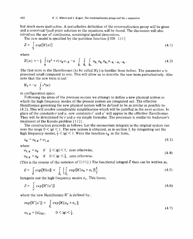
The new modelis specifiedby the partition function [108—111]

Z ~exp{lC[a]} (4.1)

where

~C[a] —~ f (q2 +r)aqa_q —u 5 5 5 a~,aq2aq,aq,_q2_q,. (4.2)

q ~ q2 q,

The first term in theHamiltonian (to be called ~JCF) is familiar from before.Theparameteru ispresumedsmallcomparedto one.This will allow usto describethenew term perturbatively.Alsonotethat thenew term is just

~1—u fs4(x)

in configurationspace.Following the ideasof theprevioussectionwe attempt to definea new physicalsystemin

which the high frequencymodesof the presentsystemare integratedout. The effectiveHamiltoniangoverningthe new physicalsystemwill be definedto be as similaras possibleto(4.2).This will involve considerablesimplification which will be justified in thenext section.Inplaceof theconstantsr and u, new constantsr’ andu’ will appearin the effectiveHamiltonian.They will be determinedby r anda via simple formulae.The procedureis similar to Anderson’streatmentof the Kondoproblem [112].

The constructionproceedsas follows. Let the momentumintegralsin theoriginal systemrunoverthe range0< I~i< 1. The new systemis obtained,as in section3, by integratingout thehigh frequencymodes,~ < i~I< 1. Write the functionaq in the form,

aq = ao,q + al,q (4.3)

wherea1,q = aq if 4< I~I< 1, zerootherwise,

a0,q = aq if 0 < i~I < ~, zerootherwise.

(This is thereverseof the notation of [111].) The functional integralZ thencanbe written as,

Z 5exp{~C[a]} j (I exp{~lC[ao+ai]}}. (4.5)

Integrateout the high frequencymodesa1. This leaves,

Z=5exp{~lC’[a’]} (4.6)

wherethe new HamiltonianX’ is definedby,

exp{~C’[a’]} = 5 exp{~1C[a0+ a~

(4.7)

ao,q ~a~2q), O<iqi<~.

K. G. WilsonandJ. Kogut, The renormalizationgroup and the � expansion 103

Here,as in the Gaussianmodel, a renormalizedfield a~,dependingon rescaledmomentahasbeendefined.

Thereis a correlationfunctionF~,’associatedwith the new Hamiltonian.X’; the new correlationlengthis,

= {dF’ 1}~2 (4.8)

As in theprevioussection,onewill haveF~= ~22-d F~qand~‘ = ~- ~.

The preciserelation between~Cand~C’can be workedout perturbativelyif u is small. The mostgeneral form for ~C’can be written

~J u~(q)a~,a~— $ 5 $ u’4(q~,q2, q3, —q1 —q2 —q3)a~,a~,a~,a~q1-q2 q5q ii, q2 �j, ,

+ higherordertermsin a. (4.9)

The functionsu~,u~,etc.will be determinedfrom (4.7).The simplificationsneededto put (4.9)into the form of(4.2) will be introducedlater. Write (4.7) in the form,

exp{~lC’[a’]} = 5 exp{~lC~[a]+ ~C1[a]}

exp{~W’[a’]} = exp{~C~[ao]}5exp{~CF[ai]+ ~W~[a0+ a1]). (4.10)

The termexp{~CF[aO]}canbe written trivially in termsof a’,

~CFao~f $ (q2+r)a_qaq (4.11)

0 < Iqi <~-

~Fao _~(~22~2) $ (q2 +4r)a~a~q. (4.12)0 < Iqi < 1

The nontrivial physicslies in the termsdependingon u. To obtaintheseterms,consider(4.10)andexpandexp{~lCj[a]} in powersof u. It is convenientto write this expansiongraphically.Denote(—~C

1)by a cross(fig. 4. 1 a). The four endpointsof thecrosssymbolizethe four a’s in ~lC1.

X i-x+4xx-...(a) (b)

Fig. 4.1. (a) Graphical representation of—JC1.(b) Graphs for exp@cl}.

The expansion

(4.13)

is showngraphically in fig. 4. lb. Considernow the functional integralof eq. (4.10). Using the

expansionof (4.13),onehasto calculateGaussianintegralsof the type

I(q1,.. .,q~) ~a1,q,. . . ai,q~exp{~lCF[a1]}. (4.14)

104 K. G. WilsonandJ. Kogut, The renormalizationgroup and the e expansion

This integralcanbe written in termsof the functional integral

ZF = 5 exp{~CF[al]} (4.15)

and the contraction&~~a1,q, which is

dd 2a~,qai,q, = (2ir) & (q +q1)/(q + r) (4.16)

providedthat ~< i~I< 1 (it is 0 for I~I< ~). The integralI(q1, . . ., q~,)isZF timesthe sumof allcontractions of a1, q, - . a1,~ as explainedin section3. (Thederivationof section3 for discretespin integrations applies also to functional integrals.)The factorZF contributesonly a constantindependent of a’ to ~JC’andwill be dropped(we will studyonly a’-dependenttermsin ~C’).

In the graphical expansion of fig. 4..lb each endpoint of each cross representsa variable aq.Writing aq = a0 q + a1, q~one has to consider two choices for each endpoint. Whenit representsa1, q’ it must be contracted with another endpoint representing a1 also. To symbolizethis onedraws a line connecting the two endpoints,as in fig. 4.2b. Sucha line is called apropagator.If

x(a) (b) (c)

Fig. 4.2. Firstorder

graphsafterperforminga, functionalintegral.

an endpoint represents aU q it is left as is. The functional integral in eq. (4. 10) is obtainedgraphically by consideringall possiblewaysof contractingsomeendpointsandleavingsomeendpoints uncontracted. Topologicallyequivalentgraphsare thenlumpedtogether.For examplethe integral of ~JC1itself involves the threegraphsshownin fig. 4.2. Whenoneformsall possiblecontractions on the single cross, the graph with no contractions (fig. 4.2a) occurs once, the graphwith one contraction (fig. 4.2b) occurs 6 times, while the graph with two contractions (fig. 4.2c)occurs 3 times. The diagrams that occur in second order are shown in fig. 4.3 together with thenumber of times each graph occurs (the numerical factor includes the factor ~multiplying ~1C?ineq. (4.13)).

A given diagram is calculated as follows. Consider for examplethe first diagramof fig. 4.3c.One starts with two crosses;beforeintegrationovera1 thesecorrespondto

u2 $ . . . $ (2~)dod(q+qi+q

2+q3)oqaqaqaq,

(4.17)

xj’ - . - J(2ir)d~(q4+q5 +q6 +q7)aqaqaqaq,.

For eachexternalline ~a is replacedby a a0, while for eachinternalline the correspondinga’sare replacedby apropagator.For theexampletheresult is

u2 5... $ (2ir)~(q+q

1+q2 +q3)(2ir)~’1(q

4+. . . +q7)(27r~~~d(q2+q6)q (4.18)

, (2lr)0’6c~(q3÷q7)[q~+ r]1 [q~ + r]1 a

0,qao,q, a0,q4ao,q1.

K. G. Wilsonand .1. Kogut, Therenormalizationgroup and the � expansion 105

with iqi, iq1I, iq4i, and q5i restrictedto be lessthan4 while iq2i, Iq3i, iq6i, and q7i mustliebetween4 and 1. Eliminatingall the 6-functions,andputting in the numericalfactor36, onehas

36 5 J j a0,q 0~,q, 00, q4 a0, —q —q, —q4 J q~±r (q + q1 + q2)2 + r (4.19)

whereq2is restrictedsothat iq2l and iq +q1 +q2~lie between~ and 1. 1

The expression(4.19) is thecontributionof onediagramto theintegral J 0, exp{~1CF[ar] +

~JC1[00 + a11} of eq. (4. 10). Otherdiagramsarecalculatedsimilarly. Howeverwhat onewantstocomputeis ~W’[a’].This requirestaking the logarithmof the integral andreplacing0~by a’. Thiscanbe donewithin the diagrammaticframework.Takingthe logarithmof the integralis equivalentto removing all disconnecteddiagrams.In secondorder in u, the disconnecteddiagramsarethoseof fig. 4.3a.Thus,to secondorder in u the logarithmof the integralinvolves thediagramsoffig. 4.1 plus thoseof figs. 4.2a—4.2c.This is easily checkedexplicitly. It is straightforwardbuttediousto verify that if ~fC~is the sumof all connectedgraphsto all ordersin u thenexp{~C~}is thesumof all connectedanddisconnectedgraphsto all ordersin u.

4{x+69+33}~x+69+33} 36)~4-45-~---~_ +8—f-—f

(a) (ci

46 -e- + 72 + 72 + 36 cx~o+ 2(b) Id)

Fig. 4.3. Secondorder graphs after a, integration.

Sincewe shallstudyonly a’-dependenttermsin ~C’[a’] the graphswithoutexternallines(seefigs. 4.2cand4.3d)will alsobe dropped(onewould haveto keepthesegraphsto calculatethefree energyitself, but they areirrelevant if onecomputesonly the spin-spincorrelationfunction).Finally, replacing0~by a’ simply meanssubstituting~ for an externalline insteadof a

0,q~Onethenhasto makea changeof variablesfrom q to 2q in order to put 1C’ in the form of eq. (4.9).

Onecanwrite a setof rulesfor computinganydiagram:1. Label the momentain the “incoming” senseat eachvertex.2. Internalmomentarangefrom 4 to 1, externalmomentarangefrom 0 to 4.3. Associatea propagator(2ir~’5~~)(q1+ q2)/(q~+ r

2) with eachinternalline (q1 andq2 are

the two momentumlabelson that line).4. Associatea factoru(2~r)~~~d)(q1+ q2 + q3 + q4) with eachfour-point vertex.5. Associatea spin variable~o,q = ~0~q with eachexternalleg.6. Integratefq overinternal andexternalmomentaaccordingto rule 2.Writing explicitly only someof the diagramsin figs. 4.2 and4.3, the functionsu~,u~,etc. in

the new interaction~C’(eq. (4.9)) are:

u~(q)~22~{~q2+r+ 12u ~p2 ~r —96u2 ~ (p2 +r) (p~+r) [(~q—p—p

1)2 +r}

(4.20)

q2, q3 q4) = ~.+42-3d — l2u

2 5 2 1 1 1 2 —2 permutations..~(p +r)[(~q1+~q2—p)+r]

(4.21)

106 K. G. WilsonandJ. Kogut, The renormalizationgroup and the � expansion

q2 q3 q4 q5 q6) = _~+625du2 { + 0.8 i 2 + 9 permutations...}. (4.22)[(2 q1 2 q2 + ~q3) + r]

The momentai~iand mi arerestrictedto lie between~ and 1. Likewise onemusthave

4 <14q—p p~i<1, ~ < 14q1 + ~q2 + ~q3I < 1, etc. (4.23)

So far the discussionhasbeengeneral.Now someapproximationswill be introducedtosimplify the effectiveHamiltonian to the form (4.2). Theseapproximationswill be good fordimensiond near4, but this will only becomeapparentlater. First calculateu~(q)only to orderu.Onecanwrite

u~(q)= q2 + r’ (4.24)

provided that

~=21+dh/2 (4.25)

as in the preceeding section. We will further simplify (4.23) by making the approximations

c I I 1J 2 j l~c

~<)pI<lP +r l+r ~<pi<1 l+r

wherec = 4 f,, 1 with~<IpI< 1, and

ç 1 1 1 1 1 ____J 2 1 1 ~‘ j 1=c

<~ <~ (p + r) [(~q1 + ~q2 —p)

2 + r] (1 + r)2 ~< p1< 1 (1 + r)2

If we abbreviateu~(q1. - . q4) by u’, (4.23) becomes

r’ = 4[r + 3c j—~-----~+higherordersin u,

r 1 (4.26)u’ = 2

4’~iu—9c i + higherordersmu.L (l-l-r)2J

Finally u’6 andhigherorder termswill be ignoredin this section.A discussionof the validity of

theseapproximationswill occupythenextsection.Now eq. (4.26)will he studiedas an exampleof the RenormalizationGroup atWork. (Theseequationswerestudiedin [1131.)

4. 1. Simplifiedrenormalizalion group transformation

The first point to understandis that eq. (4.26) is to be iteratedmany times.That is, if theparametersof the initial interactionareu = u0 andr = r0, thenoneuseseq. (4.26) to define asequenceof interaction parametersul andr1, correspondingto a sequenceof effectiveinteractions~C1.The effectiveinteraction~JC1is the resultof integratingall spin componentsaq with2 <iql < 1 in the original interaction.The effectiveinteraction~C1describes the behavior ofspin components

0q with 0 < i~l<2-1. Eqs. (4.26)now read

r1~1 4{ri+3cu1/(l +r1)} (427)

Ul+ 1 = 2~—d{u, — 9c u?/(l + r,)2}

neglectinghigherordersin u1.

K. G. WilsonandJ. Kogut, The renormalizationgroupand the � expansion 107

4.2. The c-expansionanda non-tn vial fixedpoint

Considernow the fixed pointsof (4.26).At a fixed point (r = r*, u = u*), onehasr’ = r and= u, which implies that~‘ = ~. However,we havearguedbeforethat ~‘ = 4 ~, soat a fixed point

the correlationlength mustbe infinite, i.e. we mustbe at a critical point of the theory.(Anothersolution is ~ = ~‘ = 0, but this possibilitycanbe ruledout by otherconsiderations.)It is clearfrom(4.26)that a trivial fixed point r* = u” = 0 existsas in the Gaussianmodel.We will seebelow,however,that the interactionsin the presentmodelcan generatemoreinterestingpossibilities.

First imaginethat thenumberof dimensionsof the system,d, is greaterthan4. If (4.27) isiteratedmanytimesa1 approacheszero,andif oneapproachesa fixed point it is the trivial point

= u” = 0. Soto getmoreexciting results,supposed <4 andu0 is chosensmall. Upon iterationu1 will increasewith 1 until the secondtermsin (4.27)becomecomparableto the first. In thiscasea new, nontrivial fixed point emerges.The fixed point (u*, r*) is given by,

u~ ~— (24d — 1) r* —4cu~. (This assumesr* ~ 1.) (4.28)

If d ~ 4, u” andr* arebothsmallandour approximationsarereasonable.(Seethenext section.)Define

e’4—d. (4.29)

Then,the position of the fixed point for smalle is

u*~ e1n2, r*~_~eln2. (4.30)

Imaginebeginningthe iterationscheme(4.27)with u0 > u*. Subsequentvaluesof a1 willdecreasetowardsu’~(fig. 4.4a). If u0 <u”, subsequentvaluesof u1 will increasetowardsu’

1’(fig. 4.4b).Therefore,thevalueof u occurringin the Hamiltonianafter manyiterationstepsis

un+l un+l

.__un+I~un ,,,un+e’un,

u* Uo ~fl u0 u~

(a) (b)Fig. 4.4. The iteration formula for U~. If u0 > u*, the iteration scheme(a) leadsu~to u* from above. If u0 <us, u~approachesu~from below (b).

nearu* no matterwhatu0 was.Thismeansthat the fixed point valueu* determinesthe strengthof the couplingamongthelong wavelengthfluctuationsin thesystem,independentlyof thevalueof a0.

4.3. Linearizedequationsandcalculationof v

Now the calculationof v will be discussedusingeqs. (4.27).This is somewhatmorecompli-catedthan in previousexamplesandwill be workedthroughin detail.Seealso [114] and [1111.

108 K. G. Wilsonand J. Kogut, The renormalizationgroup and the � expansion

First it is useful to comparethesolutionsof the recursionformula(4.27)with thecorrespondingrecursionformulaof the Gaussiancaser1~1 = 4r1. In theGaussiancaseonehastwo typesofsolutions.If r0 = 0 then r = 0 for all l: This is the fixed point solutionandcorrespondsto the caseT = T~.If r0 ~ 0 thenr1 = 4

1r0 andr1 -~ no forl-~’oo~This corresponds to the case T ~ T~.For T

near7~,r0 is linear in T—Tc.One complicationof the non-Gaussiancaseis thatonecanbe at the critical temperatureT = Tc

without havingr0 andu0 equalto the fixed point values.The reasonis thatonehasto fix onlyoneparameterT to be at the critical temperature, while one must fix both r0 = r~andu0 = u* tobe at the fixed point. Thus one can imagine that for any value of a0, there will be a critical valueToc for r0 (roc will depend on u0) which corresponds to T = T~.The role of the fixed point forT = 7~is that r1 —~ r* and u1 —~ u * as 1 —~ on (If T ~ T~,r1 and u1 will have another limiting behaviorfor large 1.)

Suppose one is considering a specific starting interaction with T the only variable. Then= r0(T) and u0(T) will depend on T in a specific analytic way. (See, e.g. (3.29).) Write

ro(Tc) roc, uo(T~)= U0c. Wewant now to study the theory for T near T~,in order to calculatetheexponent~. The first stepis to study the sequence{ri(T), ui(T)} generatedby iterating(4.27)starting from r0(7),u0(T). Examples of these sequences are shown in fig. 4.5. Weexpectri(T~)~ r*, u~(T~)~ u* as l —~ no (line A of fig. 4.5). Since the recursion equations are analytic,one also expects r1(T) = r,(Tc) + (T Tc)r(Tc) (and similarly, for u1(T)) for fixed land smallenough T—T~.Ifl is sufficiently large ni(T~) r* so r,’(T) is also close to r*.

r

— o•• UQC

0•\~

A

Fig. 4.5. Plot of the iteration schemefor threedifferent initial choicesof parameters. SequenceA(T = Tc) goesinto the fixed point (u*, r*).SequencesB and C begin for choicesof u and r

slightly removed from criticality. Thesesequenceseventually deviate far from the fixedpoint but approach the unique curve D.

Thissuggeststhat we studythe recursionformulaefor the caser1 r*, ui u*. In this caseonecanlinearizethe recursionformulae.The result,in matrix form, is

rri+i_r*1 rri_r*I i I (4.31)[ui+i_u*j [u1_u*

K. G. WilsonandJ. Kogut,Therenormalizationgroup and the e expansion 109

where

— l2cu* 12c(l+r~)2 l+r*

M= . (4.32)2~. l8cu*2 �1 l8cu*1

+ (1 +r*)3 2 [1 (1 +r*)2]

It will be usefulto know the resultof iteratingthe linearizedrecursionrelationmanytimes.The result is, formally

rri+ ~_r*l rri_r*I =M~ I . (4.33)

LUI+n _r*J Lui_u*

Theadvantageof studyingM~,with n large, insteadofM itself is thatM’1 is completelydominatedby the largesteigenvalueofM. The eigenvaluesofM areeasilycalculated.In the limit u* —~ 0, theeigenvaluesare4 and 1; hencetheeigenvalues of M’1 are4’~and 1; clearly the eigenvalue4!?dominates.

We needtheexplicit form of M~neglectingthe eigenvalue1. This is easilyobtainedonceMhasbeendiagonalized.The diagonalizationis complicatedbecauseM is not symmetric;the resultcanbewritten as follows

M,1 = A1w11v11 + A2w12v21 (4.34)

where w11 andUli areeigenvectors(with eigenvalueA1) of the matricesM andMT, respectively.To

be specific,

~ M,1w1~= Akwik, ~ O/,~iM1/= Xkvk,, (4.35)

andtheorthonormality relationis

V~jWfl=5kl~ (4.36)

Not every asymmetric matrix has a complete set of such eigenvectors, but for the matrix M theeigenvectors can be constructedexplicitly. (Seetable4. 1.) In terms of w and v and A, one has

(M’7)11 = ~ XZW!kvk!. (4.37)

Table 4.1Eigenvaluesandeigenvectorsof the matrixM (to order e)

A, “4—j.e1n2 X21—�ln2

r 1WI~\ ) vl=L -

0 4c(1+ eIn2)

r—4c(1+1e1n2)1 10w2=i I 02=1

L 1 J

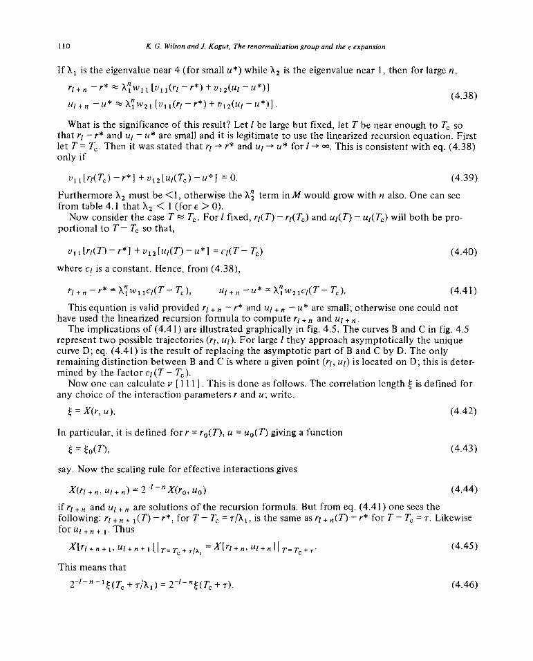
110 K G. WilsonandI Kogut, The renormalization group and the e expansion

If A1 is the eigenvalue near 4 (for small u*) while A~is the eigenvalue near 1, thenfor largen,

nj+n_r*~A’~wii[vii(ri_r*)+vi2(ui_u*)] (438)

Ul+n u* ~A’w2l[vii(rl_r*)+vl2(ul_u*)].

What is thesignificanceof this result? Let / be large but fixed, let T be nearenoughto Tc 50

that r1 — r* andu1 — u* aresmallandit is legitimate to usethe linearizedrecursionequation.Firstlet T = Tc. Thenit was statedthat r1 —~-r* anda1 —- u* forl—~-no~This is consistentwith eq. (4.38)only if

vii[r1(Tc)_r*I+v12[ul(Tc)_u*] 0. (4.39)

FurthermoreA2 mustbe <1, otherwisetheA~term in M would grow with n also.Onecanseefrom table4.1 thatA2 < 1 (for �> 0).

Now considerthe caseT ~ Tc. For / fixed, ri(T) — ri(T~)and u1(T)— ui(T~)will bothbe pro-portionalto T— T~so that,

vii[ri(T)_r*]+v12[u1(T)_u*] c1(T—Tc) (4.40)

where ci is a constant. Hence, from (4.38),

r14.n_r*_A’~wiici(T_Tc), ui+n_u*~A~w2jci(T_Tc). (4.41)

This equationis valid provided r1 + ,~ — r* anda1 + n — u* are small;otherwiseonecould nothave used the linearizedrecursionformulato computer~+ ,~andu~+ n~

The implicationsof (4.41) are illustrated graphically in fig. 4.5. The curves B and C in fig. 4.5representtwo possibletrajectories(r1, a1). For large1 theyapproachasymptoticallythe uniquecurveD;eq. (4.41) is the result of replacingthe asymptoticpart of B andC by D. TheonlyremainingdistinctionbetweenB andC is whereagiven point (r1, a,’) is locatedon D; this is deter-minedby the factor c,’(T— Tc).

Now onecancalculate ~‘ [111]. This is doneas follows. The correlationlength~ is definedforanychoiceof theinteractionparametersr and a; write,

= X(r, u). (4.42)

In particular,it is definedfor r = r0(T), u = u0(T) giving a function

= ~0(T), (4.43)

say. Now the scalingrule for effectiveinteractionsgives

X(ri+n, u,÷~)2_~~?X(ro,a0) (4.44)

if r1 +,, andu1 + n aresolutionsof the recursionformula. But from eq. (4.41)oneseesthefollowing: r1 + n + 1(T) — r”, for T — T~= r/A1, is the sameasr1 + ~(T) — r* for T — Tc = r. Likewisefor a1 + ,~+ ~. Thus

+1’ ul+fl+1~tT.T+TIX = X[ri+~, ttl+flJITT+. (4.45)

This meansthat

2l_�1_1~(T~÷r/A1)=2_l_n~(T~+T). (4.46)

K. G. Wilson andJ. Kogut, Therenormalizationgroup and the eexpansion 111

Now if

~(Tc+ r) czr~ (4.47)

onehasfor arbitrarily smallr:

(r/A1)” 2(r”). (4.48)

Thisequationcanbe true only if

= 2, (4.49)

i.e.,

p = ln 2/ln A1. (4.50)

To ordere this gives

v In 2/(2 ln 2—4 e in 2) = 0.5 + + 0(62).

A few remarksaboutthisresult arein order.The artificial featuresof the iteration scheme(namely,the factorsof log 2) do not appearin v. This is crucialsincep shouldbe property of thephysicalsystemandnot of the methodof solution! Also, for non-zeroe,v differs from theGaussian(meanfield) model. Hence,the modelstudiedin this sectionis an examplein whichinteractionsplay a role in determiningthe critical behaviorof a physicalsystem.The valueof ~ isdeterminedthrough(4.50) in termsof the largesteigenvalueA1 of the matrix M. This is similarto theresultsof section2. In section2 the 2 x 2 matrixM is replacedby a 1 x 1 matrix with asingleeigenvalueA (see(2.26)).Analogously,the equationof section2 for v (2.29) is obtainedfrom (4.50)by substitutingA for A1. Finally, notethat a is independentof the initial constanta0.This is anexampleof the universalityhypothesisdiscussedin section 1.

5. The s4 model (cont’d.)

In the precedingsectionthe renormalizationgroupequationsweremutilatedin orderto arriveatresultsquickly. In this sectionthe renormalizationgroupequationswill be studiedmorecare-fully. The endresult will be that thesimple equationsof the precedingsectionarecorrecttoorder� = — d. The discussionwill be in two parts.First, abstractgeneralizationsof thesimplified equationswill be examinedto find out which generalizationscould causetrouble.Thenthe correctrenormalizationgroupequationswill be examined.

5.1. Irrelevantvariablesand the � expansion

The recursionformulaeof the precedingsectionwere,

r’ 4[r+ 3cu/(l + r)], u’ 2~[u—9cu2/(l+ r)2] (5.1)

wherec = 4 — d andd is the dimensionalityof the system.Theseequationspossessa fixed point,

u*~~~�1n2, r*_~eln2 (toordere). (5.2)

112 K. G. Wilson andJ. Kogut, The renormalizationgroup and the � expansion

Supposethat the true equationshadoneothercouplingconstantw. Therewill thenbe anotherequationfor w’. Supposethat (at leastnearthe fixed point) the equationfor w’ is,

w’aw (5.3)

where a < 1. Then,when (5.3) is iterated,w’-~0 andthe variablew disappearsfrom the problem.w is thenreferredto as an irrelevant variable with respectto the fixed point for which (5.3) istrue. The term “irrelevant variable” is not to be takenliterally; the meaningof “irrelevant” incritical phenomenais complicated,but should be clarified by this and subsequentsections.Foranotherdiscussionof irrelevantvariablesandfixed points,see [1141.The term “irrelevantvariable” is due to Kadanoff [115].

Now we want to know whenthe presenceof irrelevantvariablescanchangethe fixed point(5.2). Supposethat the equationfor w’ is,

w’ = + (secondorder terms like a2, aw, w2, etc.). (5.4)

In particular, we forbid the appearance of a term linear in a in (5.4). (w is still classifiedas anirrelevant variable: second order terms are to be ignored in determining whether w is relevant orirrelevant. A term proportional to a can only appear in the formula for r’ or a’ since the only

diagrams linear in u are figs. 5. la, b.)

p ><(a) (b)

Fig. 5.1. Diagrams linear in u.

Considerthe fixed point of (5.4).Obviously,

w” = 0(62) (5.5)

assuming that (5.2) does not fail so that u~= 0(e). We mustnow askwhether(5.5) can invalidatethe eq. (5.2) for u* andr* if termsinvolving w should appearin (5.1). Only termsof order� areimportantin theequationfor r*, sow’~’ is negligible.However, thea equationinvolves �2 termsin an importantway. Therefore,if w appeared linearly in the u equation,(5.2) would be modifiedin an importantway.

Now considerthe casethat the w’ equationhasthe form,

w’ = w + termsof orderu3, u2w, etc. (5.6)

In this casew” O(e~)andevenif w appeared linearly in thea equation, it could not influencethe validity of thatequationfor smalle.

Theseconsiderationsshowthat the simpleequationfor a’ canbe invalidatedif thereis anirrelevantvariablew such that both (1) w’~’‘-~ 0(62), and(2) w entersthea’equationlinearly. Wewill now arguethat this possibilitydoesnot occur for theexactequationsdefinedin the previoussection.In the exactequations,the interaction(aftersomeiterations)hasthe form

~IC= —4 5 a2(q)aqaq — 5 5 $ J 6 (q1 + q2 + q3 + q4)u4(q1,q2, q3, q4)aq,

0q2

0q, aq4

q q, q2 q3

— (6th order term) — (8th order term) — . . . . (5.7)

K. G. Wilson andJ. Kogut, The renormalizationgroup and the e expansion 113

As discussedat lengthin the previousseveralsections,we integrateout thehigh frequencymodesin this system.After the appropriaterescalingof momentaand fields, a primedsystememergeswhich is describedby a Hamiltonianidenticalin form with (5.7),but expressedin termsofprimedquantities,

~c’—4 Ju~(q)a~ia~..q— $ $ $ 5 ~q q, q

2 q, q4— (6th order term)’ — . . . . (5.8)

The relationsbetweenthe a anda1 follow by the techniquesillustratedin section4 (assumingu2(p) depends only on ~.ii= p becauseof the rotationalsymmetryof theseequations):

a~(q)= ~2 2d {a2(4 q) + 12 5 a4(~q, — 4q, p’ + (second order term) +..a~(p)

u~(qi,q2,q3,q4)~423d~a4(4q1,4q2,4q3,4q4)

—12 5 u4(4q1,4q2,p, —4q1— 4q2—p)u4(4q3, 4 q4,—p, — 4q3 — 4q4 +p) + perms.u2(p)a2(4q1+4q2+p)

+15 fu6(4q1,4q2,4q3,4q4,p,p)~u2(p)

\_k6’~r~5d ,‘l Iu6~q1,. . ., q6, — ~. ~a6~2q1,- . ., 2q~, (5.9)

ii 1 1 ~1 ~1 _1 ~ ci 1 1 1 ~ 1u4~q1,~q2,~q3,~q1 2q2 2q3ja4~2q4,2q5,~q6, ~q4 2q5 2q6u2(4q1+4q2+4q3)

Whenever u2 appearsin a denominator,its argumentmustlie between4 and 1, e.g.4 <p < 1, etc.Clearly the systemof equations(5.9) is intractable.The equationfor u~in particular is a non-linear functionalequation.Therefore,thecontentionthat (5.9) canbe replacedby algebraicequations(5.1) (to lowestorder in e) is extremelyimportant.The proof thatthe algebraicequationsaresufficient to determinethe fixed point r*, a*, restsheavily on the characterofthe irrelevantvariablea6.

An exactfixed point of(5.9) is a setof fixed functionsa~’(q),u~’(q1,. . ., q~),a~’(q1,. . ., q6),etc. To testwhetherthe simpleequationsarea valid approximation,we will supposethat to ordere thesefixed functionsreduceto two fixed constantsr* andu”, namely,

a~(q)= r* + q2 + 0(62)

(5.10)

u~’(q1,. . ., q6) = O(e2)

etc.The consistencyof thisassumptionwill beverified below.First considerthe a2 equation.Write

a~(q)q2+r*+v~(q) (5.11)

wherev~(q)is a remainder.The parameter~ will be adjustedto ensurethat the coefficientof q2is unity. Let (5.10) representan expansionaboutq2 = 0, so that

v~(q)‘-‘q4 .0(62). (5.12)

114 K. G. Wilson andI. Kogut, Therenormalizationgroup and the � expansion

Substituting(5.11) into the equationfor u2(q) gives,

q2 +r*+v~(q)=~22~{~q2+r*+v~q)+ 12 $ ~ .}. (5.13)

a2(p)

Now, to order� the. . . is negligibleandthelast term reducesto

l2u* 5 1 +0(62). (5.14)p P

2 + r’1’

The parameter~ is to be determined(asin previoussections)by the requirementthat termspro-portional to q2 in (5.12)match.Thisgives

~.22_d4+0(62) (5.15)

(Thereis morediscussionof ~at the endof this section.)Now onehasan equationfor r’1’,

r* 4{r*+ 12u* f~2~+ +O(e2)) (5.16)

andan equationfor the remainderv~(q),

v~(q)= 4r4’(4q)+ e2F~(q). (5.17)

In this equatione2F~’simply representsthe correctionsfrom higherorder termsin (5.13)(withconstantand q2 terms subtracted). Suppose that F~is known; a seriessolutioncanbe written forv~’(q)in termsof F~’(q):

= ~2 ~ 22~F~(2~q). (5.18)

This is a solutiononly if the seriesconverges.However,F~’was constructedsuchthatF~’(q)‘-‘ q’.Therefore,the nth term in (5.18) is of order,

e222t1 q4/24t’22’2e2q4 (5.19)

andthe seriesconverges.Thereforev~ 0(E2) as supposed.Whatis theconnectionof this discussionwith irrelevantvariables?To seethis, expanda

2 inpowersof q,

a2(q) = r + q2 + w

1q4 + w

2q6 +... . (5.20)

Then,(5.17) gives to lowestorder

w~j~w1, w~~w2 (5.21)

andall the variablesw1, w2, . . . are irrelevantvariables.It shouldbe clearnow that v~’ cannotupsetthe simpleequationsfor r* anda*, sinceit

appearsonly in the termswith propagatorsin (5.9).Thesetermsare already0(62), so thepresenceof v~’leadsto corrections‘—O(�~)which canbe ignored.

The discussionof u4 parallelsa2. We beginby writing,

a(q1,. . .,q4)u*+r4(qi,. . .,q4) (5.22)

K. G. WilsonandI Kogut, Therenormalizationgroup and,the � expansion 115

wherev~is a remainderdefinedsuchthatv~’(0.. . 0) = 0. Then, substituting(5.22) into (5.9) andusing(5.15),we canobtainequationsfora* andv~(q1,. . .,

~ a*2 ~ •*(~J0 0 0 ‘~

= 2~a*_36 J + 15 j ~ ‘ ‘ ‘ ~ (5.23)~ (p2 + r*)2 p2 + r’1’ 3

., q~)= 2~v(4q1,. . .,4q~)+ e

2F’(q1, - . ., q4). (5.24)

The . . . termsin the equationfor a~areall of orderc~or higherandcanbeignored.Eq. (5.24)implies that v -~0(62) in thesameway that (5.17)gavev~ O(e2). Sincev doesnot appearlinearly in the equationfor a*, v cannotinvalidate the simpleequations.

Now considera6. Sincea6 appearslinearly in thea* equation,it is potentiallydangerous.Considerthe equation(5.9) for a’6 and the term correspondingto thediagramin fig. 5.2 inparticular.Thisterm appearsonly whenthe internalline carriesmomentumgreaterthan4-, i.e.

I2q1~~q2+~q3I>~. (5.25)

However,it is only a6(0,0, 0, 0, p, —p) which appears in the a” equation.This correspondsto= q2 = 0, q3 =p in fig. 5.2. In order to satisfy(5.25) i~imust beprecisely I (seefig. 5.3). This

is only onepoint in the integralover~i in (5.23) andthereforedoesnot contributeto u*. There

(2

Fig. 5.2. Diagramcontributing to Fig. 5.3. The only diagramcontributingu6(q,,...,q6). to u6 and entering the u* equation

linearly.

areothergraphswhich contributeto u6(0, 0, 0, 0, p, p) for ipi < 1 but theseareof order ~3; thusa6 doesnot contributean~2 term to the a* equation.~Therefore,the a* equationis safe!

Finally, we mustcastthe a* equationinto the form we hadlast section.In particular,sincer* 0(e)anda* 0(c), we canreplace,

a*2 1

J(p2+r*)2 =a J~+O(e) (5.26)

andif we redefinethe constantc of section4 to be

c4 .1-4- (5.27)

we find that (5.23)reads,

= 2~{a*— 9ca*2} (5.28)

which hasthesameform as (5.1) if we likewiseneglectthe r in thedenominatorof the second

tme equation for u6hasa term linear in u5, so if u3 were of order �2 then 06 would bealso. But explicit study of the equation

for u8 showsthat u8 isof order e~.

116 K. G. WilsonandI Kogut, The renormalizationgroup and the e expansion

term of (5.1). Now, we turn to the equationfor r*. In particular,to calculatea oneneeds(5. 16)for smalldeparturesfrom the critical point. Onegets:

r’_r*=4{r_r*_l2a* j(2~~2)(r_r*)+...). (5.29)

We mayapproximate,

J (p2 +r~)2= I -~ + 0(e) = +c ÷0(e) (5.30)

and rewrite (5.29),

r’_r*~4[l_3a*c](r_r*). (5.31)

Sincethe sameconstantc appearsin both (5.28)and(5.31), it will cancelout in the calculationof the critical exponentaas in section4. Therefore,we haveshownthat(5.1) sufficesto lowestorderin e in determiningthe critical exponent.

5.2. Completerenormalization group transformation

Whatoneseesfrom this discussionis that the exactrenormalizationgroupequationsarenothopelesslyintractablefunctionalequations.To order � they reduceto simplealgebraicequationsfor two parametersr” anda*. The basicreasonthatmadethis simplificationpossiblewas the“iterability” of the equations for the remaining functional variables v~’(q),v(q, . . ., q

3), etc.That is, if the correctiontermsF~’(q)in the equationfor v~(q)areknown,and are of order�2,

thenv~(q)canbe computedexplicitly from (5.18)andis alsoof order~2 This is in contrasttotheequationfor a*, in this casethesecondordertermsareof order�2 but thesolutiona* is oforder e.

The iterability of the equationsfor thevariablesv~(q),etc. ensuresthatonecanconsistentlycalculatethe exact fixed point a~’(q),a(q, - . ., q~),etc. to higherordersin e. Thenthefunctionsv~(q),etc. cannotbe neglected;but no newproblemsarisein calculatingthem(exceptpossiblysomedifficulties with integrationsin non-integraldimensiond). This is becauseonecanarrange a calculation so that the diagrams contributing to v~(q),etc. (i.e. the functionF~(q))areknownto anygiven ordere” beforev~(q)itself is calculatedto ordere’~.The iterability ensuresthenthatv~(q)existsin order�~.

The iterability of theequationsfor v~’(q),etc. is a consequenceof the fact thatthesefunctionscanbe expressedentirely in termsof irrelevantvariables.For example,we showedthat if v~(q)iswritten w~q

4+ w~q6+ . . . thenthe equationsfor w~’, etc. areof the form

wr = aiwT + secondorderterm,(5.32)

w~= a2w~+ secondorder term,

etc. wherea1 < 1, a2 < 1, etc. The fact that a, < 1 makesit possibleto solve theseequationsforwr andw~if the secondordertermsareknown.

Iterability is possibleevenfor relevantvariables:in particular,the equationfor r* is alsoiterableif onewritesit

= 4r~+ otherterms. (5.33)

K G. Wilsonand I Kogut, The renormalizationgroup and the e expansion 117

Thenonecanalsosolve for r*. It is only equationslike the equationfor a*:

a* = a3a* + otherterms (5.34)

with a3 = 1 + e which is not iterable,becausea3 is too closeto 1. d 2

Finally, considerfurther theconstant~. In all calculationsso far ~2 hasturned out to be 2 +

independentof c. But in a higherordercalculation~ will change.The equationwhich determines~. is,

q2 = 2~~2{~q2 + (q2 termsfrom all diagramscontributingto a

2)}. (5.35)

The lowestorderdiagramwhich hasq2 dependenceis shownin fig. 5.4. This diagramis of order

Fig. 5.4. Lowest orderdiagramwhich affectsthe value of (~.

so ~ will haveto havea compensatingterm in order62. It will be shownin section7 that thevalue ~* of ~at thefixed point determinesthe critical exponentri. The formulais

~=d+2_2ln~*/ln2. (5.36)

6. The approximaterecursionformula

This sectionis devotedto the approximaterecursionformula[Ill]. The approximaterecursionformula is an approximationto the renormalizationgrouptransformationdiscussedin sections4and5. It will be usedto provideorder-of-magnitudeunderstandingof therenormalizationgroupfor 2 <d ~ 4 andwill shedlight on the validity of the e expansion.

The extradegreesof freedomin the exactrenormalizationgroupequations,as comparedtothe simpleequationsfor r anda, areof two types.First of all, therearemomentumdependentfunctionslike a

2(q)anda4(q . . . q3) insteadof discreteparametersranda. Secondly,therearean infinite setof functionsa2, a4, a6, a8, etc.,correspondingto all powersof thespin variable,not just a2 anda4. The approximaterecursionformulatakesinto accountall powersof thespin,but doesnot allow momentumdependenceexceptin a2. Most importantly for thisreport, theapproximaterecursionformulaincludesFeynmangraphsof arbitrarily high ordersandin sufficientnumberso that the divergentnatureof the Feynmangraphexpansionis preservedby the recursionformula.This meansthe recursionformulacanbe usedas a model to seehow badly the higherordergraphsaffect the � expansionwhencalculated,say,in 3 dimensions.

The approximaterecursionformulawas first obtainedby functional integraltechniques[1111.Herea moretransparentgraphicalderivationwill be given due to Polyakov [116].

6.1. Polyakov’sderivation

Consideran interactionof the form

~ =~4 c{vis(x)}2 —ci J Q[c2s(x)] (6.1)

118 K. G. WilsonandI Kogut, The renormalizationgroup and the e expansion

wheres(x) is our usualspin field andthe functionQ is definedthroughits expansion,

Q[y] =ry2+uy4+wy6+... . (6.2)

Two constantsc1 andc2 havebeenintroducedin ~Candwill be adjustedsothat the recursion

formulawill be free of certainphasespaceintegrals.Note thatthe only momentumdependencein ~Wappearsin its first term,i.e. no gradientsareallowedin the expression(6.2). As usual,wearegoing to force the renormalizationgroupequationsto producean effectiveHamiltonian~C’with the sameform as K. That is, with the helpof someapproximationsone triesto produceaneffectiveHamiltonian~C’of the form

, r ~ 2 ~~lC=—-~- j Vh’(x) ~Ci j Q [c2s(x)] (6.1 )

(c1 andc2 arethe sameconstantsas appearin ~C)wheres’(x) is the effectivespin field obtained

by Fouriertransformingo~the field c%’ is as in previouslectures

flq = ~Uq’/2

and~C’is definedby integratingout the componentsffq with4< qi < 1. The only differencebetweenthe approximaterecursionformula to be derivedhereandeither theexact or simpleequationsof sections4 and5 is thatdifferentapproximationswill be made.

To illustrate the approximationsto be madeconsiderthegraphin fig. 6. 1 which contributesto a’. The prescriptionfor neglectingmomentumdependencewill be to arbitrarily set the

Fig. 6.1. A graph contributing toto u’ in the approximaterecursion formula.

momentumof the externallines to zero.This is not an absurdideabecausethe externallineshavelower momenta(i~i<4) thanthe internal lines(i~i>4). So, the approximationgoesinthe right directionanyway.Now, fig. 6.1 gives the following contributionto a’:

36 (1 2( 4~2 1 24-d . (6 3)a kclc2, (p2 + 2rcic~)2J —c

1c~

The factorsof c1c~multiplying a in (6.3) appearbecausethey appearmultiplying a in theinteraction(6.1): to fourth order in s(x),~ICis

J [Vs(x)]2—rc

1c~ 5s2(x)_acic~ $s4(x)+. . . . (6.4)

The factor2~-d = ~ appearsin (6.3) as a resultof the definition of a,~as discussedinsection4 and thevalueof~(4.25);and finally, the last factor(—c1c~)

1appearsin (6.3) becausethe strengthof the s’(x)4 termin ~C’is —a’c

1c~,so to obtainu’ onemustdivide by —c1c~.In

K. G. Wilson andJ. Kogut, The renormalizationgroup and the � expansion 119

developingtheapproximaterecursionformulacontributionssuchas (6.3) are simplified furtherby applyingthe following two rules:

1. Replacep2 in the integrandby an averagevaluep~.2. Replacethe integralf~~4<i~i< 1) by a constantP.

Clearly, suchsimplificationsarenot necessaryin discussingrelativelysimple graphssuchasfig. 6. 1. However,the neglectof the precisemomentumdependenceof the internallineswillallow oneto calculategraphsof arbitrarily high order.

Yet anothercalculationalrule is imposed,3. Only evennumbersof internallinesareallowedateachvertex.

The primarypurposeof this rule is to excludegraphsof the form shownin fig. 6.2. Suchgraphsshouldnot appearin the physicaltheorysincetheydo not conservemomentum.However, rules 1and2 by themselveswould permitsuch effects;this will be shownbelow. Rule3 alsoeliminatesgraphssuchas fig. 6.3. In the limit that the externalmomentago to zerosuchgraphsare forbidden

internal external

Fig. 6.2. A graph which doesnot appear in the approximate Fig. 6.3. A graph eliminated byrecursion formula. It is rule 3.omitted in accordancewithrule 3.

by momentumconservationso this is alsogood.Unfortunately,this rule also forbidsgraphs,suchas fig. 6.4,which shouldbe presentin the real theory.In particular,the classof graphswhich areallowedto contributeto r’ is very restrictivein this approach.It is not true,however,that all theeffectsof graphsof the typein fig. 6.4 will be lost. For example,after oneiteration the graphinfig. 6. 1 contributesto a’. In thenext iterationtwo of the externallegsof fig. 6.1 might becontractedforming a graphtopologically like that in fig. 6.4. In otherwords, within the frame-work of theserulesthe graphof fig. 6.5 would be omittedwhile thegraph of fig. 6.6 wouldappear.

4/2—I 1/2—4

ED ED ~E)4/2—1 4/4—4/2

Fig. 6.4. A desirable graph Fig. 6.5. This graph is not Fig. 6.6.This graph occurs in theforbidden by rule 3. . .accountedfor in the approximate approximate recursion formula.

recursion formula. The labels

1/2—1 indicate the momentumrangeson the internal legs.

Now we shall simply write down the approximaterecursionrelationandshow from ‘itsperturbationexpansionthat it is equivalentto therules 1, 2, and3 above.The approximaterecursionformulais,

$ dy exp[—y2 _4Q(

2i~2 x +y)—4Q(2~12 x

exp[—Q’(x)/2”] = . (6.5)

$ dy exp[—y2 —-4-Q(y) +Q(y)]

120 K. G. Wilsonand J. Kogut, Therenormalizationgroup and the eexpansion

To comparethis formulawith the rules for simplifying graphs,this formula mustalsobeexpandedin diagrams.This meanswriting out the exponentialof the numeratoras

exp{—y2 —-4-Q(y +21d/2x) —4-Q(—y + 21-d/2x)} =

exp{—(l +r)y2 _22_drx2 —uy4—6 x22duy2x2 ....24_2dax4 —. . .}. (6.6)

Onethenexpandsin powersof the quarticterms(proportionalto a) andhigher.This canbe doneby graphs,just as was donefor the exact functional integral. The ay4, 6ay2x222’Q’ andax42420’terms, for example,definethe 4-pointvertex,with uy4 corresponding to all lines being internal,the 6ay2x222~ correspondingto two linesbeinginternal,two beingexternal,etc.The pro-pagatorfor internallines is the inverseof the coefficientof 4y2 in (6.6), namely(2 + 2r)’. It iseasyto seethat the absenceof termsodd in y in (6.6) correspondsto rule 3 — removingverticeswith an oddnumberof internallines.Without rule 3 onewould havehadexp[—y2 — Q(y +

2i-d/2x)]

instead of the exponential with two Q terms,in eq. (6.5). Thenthe ry2 term in Q(y) becOmes

r(y +2~d!2x)2 which hasa crossterm rxy. This is the term correspondingto the graphof fig. 6.2

which is excludedin the exponentof eq. (6.6) andwhich is not presentin the completetheory.The variablesx andy areanalogousto the variablesuoq and

01q in the theory of section4; thereis no term of the form 0oq01~qin section4.

The denominatorin (6.5) removesall graphswithout anyexternallines (“vacuum to vacuum”graphsin field theoreticterminology).Taking the logarithmof the right-handsideof(6.5) removesall disconnectedgraphs.So—Q’(x)/2°’ is the sumof all connectedgraphswith at leastoneexternalline. Note that thex2 term in (6.6) passesthroughthe integral(6.5) and contributes4r to r’. Werecognizethis as the usual free field term which contributes4r to r’.

The mostimportantfact about (6.5) is that it producesthe samesetof graphs(apart from therestrictionof rule 3) that are generatedby expandingthe exactfunctional integral. This isbecausethe graphsthemselvesdo not distinguishwhetherthe integrationvariableis a singlediscretevariable(y) or a setof variables,or a functionvariableUq. The distinctionis madeonlyin termsof the rulesfor graphs:in the exactcasea four-point vertexstandsfor a

4(q . . . q~),forexample,while in the approximaterecursionformulathe four pointvertex standsfor u. Further-more, the topological factorassociatedwith a graph(the factor36 for the graph of fig. 6. 1, forexample)is alsothe same;it comesfrom the numberof topologically equivalentwaysof combin-ing agiven setof verticesandpropagatorsandthis is a countingproblemwhich involvesonly thegraphsthemselvesand not what theyrepresent.

6.2. Somenumericalresalts

Verification of the first two rules is now a matterof bookkeeping.Onemustshowthat thefactorsof P andp~producedby rules1 and2 canbe absorbedinto the coefficientsc1 andc2 foreverygraphin the theory.Considera generalgraph of 1 internallines,2m externallines andnvertices.In the exacttheory,this graphhasn—l deltafunctionsaffecting the momentaofinternallines,andconsequently1 — (n — 1) momentumintegrals.Therewill be 2m + 21 linesatvertices.Now onecanrecordthe factors(apartfrom the topological factor) for thisdiagram.Therewill be

1. (~cj)’1 a factor—c

1 for eachvertex.2. c~m+ 21 a factorc2 for eachline at eachvertex.3. P

1 “~ + — a factor P for eachintegral.4. (p~+ 2c

1c~rY” a propagatorfor eachinternalline.

K. G. Wilson and J. Kogut, The renormalizationgroup andthe eexpansion 121

We want thecontributionof this diagramto a coefficient in the expansion(6.2).Therefore,wemustdivide by an overall factorof —c

1 anda factorc~m(one factor of c2 for eachexternalline).Thereis finally a factor coming from the changeof scalewhich is ~2~n~— (2m — 1)d=22m—(m—1)d~

~-2 is equalto 22+d sinceno graphsarepermittedto contributeq2 termsto u

2(q) (due to rule 1).Collectingall factorsgives,

(_l)n_1C~c~m+2lP1_n+1 2 1 2 1 2m 22m—(m—1)d (6.7)(p0+2c1c2r) c1c2

In order that the dependenceon P andp~disappear,choose

C1 P, C2 =po/(2P)h/2. (6.8)

Now (6.7) becomes,

(~1)~l_122m—(m--1)d/(2+ 2r)’. (6.9a)

Considernow the samegraph in the expansionof the approximaterecursionformula. For eachexternalline thereis a factor 21 —d/2 For eachpropagatorthereis a factor(2 + 2r)’. Combiningthesefactorsfor the 2m externallinesand1 internallinesgives

22m _md(2 + 2r)~. (6.9b)

Besidesthesefactorsthereis a factor—u for each4-pointvertex,a factor —w for each6-pointvertex,etc.; thesefactorsalsoappearin the original interpretationof thegraph exceptfor the— signs. Therearealsocombinatorialfactorssuchas how manyways theinternal linescanbeassignedat a vertex(the factor6 in 6ux2y222~~in eq. (6.6) is a combinatorialfactor) or thenumberof waysof hitching differentverticesto form agiven graph.The combinatorialfactorsarethe samefor both the functionalintegralexpansionandthe expansionof the recursionformula.Thereis one final factor: the graphsfor theintegralson the right-handsideof(6.5) give_Q1(x)/2~~,not Q’(x). So to obtainQ’(x) onemultiplies by _2d~Thischangesthe factor(6.9b) to

(—1 )fl -1 22m -(m - i)d (2 + 2 r)~,

which is identicalto (6.9a).This completesPolyakov’sderivation [116] of theapproximaterecursionformula. Note that0 for the approximaterecursionformula; this follows from eq. (5.36)since~ = 2d+2 The

reasonfor this is that all momentumdependenceof graphshasbeenignored.The approximaterecursionformulais not a quantitativeapproximationto the exactrenorma-

lization groupequations.So far as is known, it is not the first term in anyexactexpansionof theexactrenormalizationgroupequations.Nor is it the first term in a sequenceof successiveapproximationsconvergingto theexactequations.One canonly judgeits validity by comparingsolutionsof the approximaterecursionformulawith othercalculationssuchas high temperatureexpansions(seesections7 and8). In this respectit doesratherwell.

Baker [117] andDyson [118] haveconstructedmodelsfor which the recursionformulaisexact.However, thesemodelscontainlong-rangeinteractionsof a peculiarsort.Golner [119] hasderiveda modified form of therecursionformulain which i~is not automaticallyzero.

The original derivationof the recursionformula[Ill] using“phasespacecell analysis”is morecompellingthanPolyakov’sderivationpresentedhere.Phasespacecell analysisis not discussedin thesesectionsbecauseit hasalreadybeendescribedseveraltimes: thoroughly in [111], brieflyin [120]. One shouldfind thesereferenceslessdifficult to readafterstudyingthis sectionand

122 K. G. Wilson and.1. Kogut, The renormalization groupand the e expansion

section7. Phasespacecell analysiswasoriginally developedin connectionwith fixed sourcemodelsof the nucleon[1211. The real importanceof phasespaceanalysisis that it is an ideaonecanuseto get startedon a problemfor which all conventionaltechniqueshavefailed. That in factwas the situationin critical phenomenaat the time [111] was written. Anotherexampleof theuseof phasespacecell analysisis given by LangerandBar-on [122].

We shallnow discusshow oneusestherecursionformulato studycritical behaviorwithoutexpandingin powersof u, w, etc.Since(6.5) is a non-linearintegralequation,theonly adequatetool to analyzeit is thecomputer.Luckily, onedimensionalintegralscanbe evaluatedwith greateaseandaccuracynumerically.The analysisof (6.5)beginswith a searchfor the fixed point [1111.Consideran initial interactionwith Q0(y) = r0y

2 +~y4.The coefficient r0 is a parameterwhich

onevariesin orderto locatethe critical temperature.To do thisonegenerateson the computerasequence

Q0(y)-*Q1(y)-+. . .-~Qi(y)-~ (6.10)

for a given r0. This sequenceis examinedfor a fixed valueof y, sayy = 1.5. Whatonewantsis asequencetendingto a limit for 1 —~ ~, asdepictedin fig. 6.7. This neverhappensin practice.If r0

+

÷+ + + + + ++

+

i i i 12123456789

Fig. 6.7. An ideal plot of the approach of

Ql to a fixed point.

is chosentoo large,the sequencegoesoff to infinity becauseoneis abovethe critical point andthe~Gaussianterm r1y

2 dominatesfor large1, andthenr1 + 1 4r1. To compensate,onelowersr0 and

generatesa new sequenceQl. If r0 were chosentoo low, the sequencewill tendto oscillatebadlyfor large1. In practiceonecompromisesbetweenthesetwo extremesby choosinganr0 suchthatQi falls within a preassignedrangeafter apreassignednumber1’ of iterations.This procedureisthenrepeatedfor largervaluesof 1’. Once onehasa sequencewith Q1(y) stabilizedovermanyiterations1’ (1’ ~ 12 in practice),onehasa goodapproximationto the fixed point functionQ*~

In threedimensionsthe resultingfunction is shownin fig. 6.8. Furtherpropertiesof therecursionformulaandthe fixed point functionQ* will be discussedin thenextsection.

-.7

Fig. 6.8. Fixed point function Q*(y) fordimension 3 as determined numericallyfrom the approximate recursion formula.

K. G. Wilson andJ. Kogut, The renormalizationgroupand the � expansion 123

7.

This sectionis divided into two parts.First is a continuationof the presentationof the resultsof investigationsusingthe approximaterecursionformula.Thencomesthe derivationof a scalingformulafor then-spincorrelationfunctions.This formulawill allow usto computee expansionsfor critical exponentsusingFeynmangraph techniques.

7.1. More results from the approximate recursion formula

Recall that last section’spresentationof the approximaterecursionformulabeganwith theinteraction

~C0=—~ J [vs(x)12 —c~J Q

0[c2s(x)] (7.1)

wherethe possiblemomentain this physicalsystemrun overthe interval0< I~I< 1. Therecursionformulathengeneratesa new interactionwhich describesthe samephysicsfor asystemwith a momentumcutoff one-halfas large.In particular,

X1 —4 J [Vs(x)]2 c

1 J Q1[c2s(x)] (7.2)

generatesthe samephysicsas (7.1) but with a momentumcutoff I~I<2_I, providedthat

Qi~10) _2d ln{I,(21_~/2y)/Ii(0)} (7.3)

where

Ii(z)= $ exp[—y2—~Qi(y+z)—-~-Qi(y+z)]dy. (7.4)

Theseformulaehavebeenstudiednumericallyfor severalchoicesof Q0 anddimensionalityd of

the physicalsystem.Considerin particular

Q0 = r1~y2+ u

0y4 (7.5)

‘for d between2 and4. As discussedat the endof last lecture,given u0 oneadjustsr0 to find the

critical value,i.e. the valuer0~of r0 for which,~ ~ Q*(y), as! (7.6)

For d = 3 andu0 = 0.5 one finds the fixed point functionQ*(y) shownin fig. 7.1. For dimensionsnear4, say3.9or 3.8 (andsmalleru0), onefinds flatter curvesas shownin the samefigure. Recallfrom ourearlierdiscussionsthatthe fixed point functionis trivial (i.e. Q* = 0) in four dimensions,so the behaviorof the curvesin fig. 7. 1 asd tendsto four is expected.Whend is precisely4, andu0 <0.35,onefinds thatu1 1/i for large1. So, free field behavioris approachedvery slowly asexpectedfrom otherformulationsof the renormalizationgroup [1231, (seesection13). Inpracticethis meansthatwhend is nearfour it takesmanyiterationsof (7.3) and(7.4) in orderto reliably mapout the fixed point function.

As d variesfrom 3 to 2, Q* becomesmuchmorecomplicated.Ford = 2, Q* behavesroughlyas shownin fig. 7.2. (This figure was obtainedfrom a slightly modified form of (7.3). Namely,

124 K. G. Wilson and J. Kogut, The renormalizationgroupandthe e expansion

~ F~2/’~ QFig. 7.1. Fixed point functionsindimension3 and3.9.Fig. 7.2. Fixed point functionin2 dimensions.This curveresultedfroma numericalstudyof a slightly modifiedform of the recursionformula.

the factor21d/2 was replacedby 21_d/2_1/8•) It is easilyseenthat two dimensionsis rather

special:Supposeoneis calculatingQi + ,(y) for largey. If d = 2, Qi+, (y) is determinedby Il(,y),i.e. the argumentsof the two functionsmatch.The behaviorof Ii(y) for largey is in turn deter-minedby Qi when its argumentis largeandcomparablein size to y. Therefore,the asymptoticbehaviorof the input function Q0 to the iterationformulawill tendto propagatethroughmanyiterations.This behavioris contraryto the existenceof a fixed point independentof Q0, andmakesit hard for a fixed point to occur. In contrast,for d> 2 the factor21 d/2 meansthat

+ 1(y) is determinedby Q~(y’)for y’ 21 _dI2~which is considerablylessthany wheny islarge.Thenthereis no problem.

Onceonehasfoundthe critical functionQ*(y), furthernumericalstudiesof therecursionformulayield the critical exponent~. For this purpose,onebegins.the iterationschemewith

r0~,but not equalto roc. One thenobserveshow Qi(y) departsfrom Q*• For reasonablylarge!, oneexpectsthat Q1 hasthe form (by analogywith eq. (4.41))

_~ Q* + (r0 _roc)X1R*(y) (7.7)

whereR*(y) is a functionindependentof l andr0. For thisto be true,1 must belargeenoughso

that initial transientshavedisappeared;thenr0 — roc mustbe smallenoughsothat (r0 — roc) X1 is

small. X is the leadingeigenvalueof the linearizedrenormalizationgroupequationas in section4.The exponent~ is,

p = ln 2/ln X (7.8)

as in section4. The eigenvalueX canbe determinedby fitting (7.7) to the resultsof the numericaliterations.

In fig. 7.3 we plot the calculatedvaluesof ~ as a function of d obtainedfrom the approximaterecursionformulaandcomparethe resultswith thehigh temperatureexpansionresultat d = 3andthe exactOnsagersolutionat d = 2. The calculatedcurveis fit well by aquadraticfunctionof � =4—d.

Anotheruseof the recursionformulais in studyingthee expansion.Onecancomputethe eexpansionfor v resultingfrom the recursionformulaby numericaltechniques.The recursionformulayields the following seriesfor 2v:

2~= 1 + 0.167e+ 0.04e2—0.0l6e3+ 0.077�~—0.2e~+ O.67e6— 2.5�~+ l0.3e~+.. . (7.9)

indicating that the seriesis really an asymptoticexpansion.If onetruncatesthe seriesatsecondorder,onefinds v = 0.603atd = 3. This is to be comparedwith the bestnumericalresultof the

K G. Wilson and J. Kogut, Therenormalizationgroup and the � expansion 125

recursionformula, p = 0.609.Keepingonly the linear term in (7.9) gives v = 0.583. Theseresultssuggestthat it is sensibleto terminatethe seriesat~2• A Padéanalysisof (7.9) alsorevealsthatthereis no appreciableimprovementoverthe �2 approximationuntil eighthorderat which pointthe Padéexpansionyields a slightly bettervalue.This suggeststhat it is importantto calculatetheexactexpansionfor v to order�2, but that thereis not muchpoint in calculatingthe �~term orhigher.The mostimportantresult from the recursionformulais the hint that the seriesto order ~2

shouldgive a good value for v for � = 1. One might not otherwisehaveexpectedthe seriesto begood for this largevalueof e.

‘-1.0 a.9.

.8 ——

a —~

.6-

I I

4 2Fig. 7.3. Critical exponentr’ plottedagainstthedimensionof thephysicalsystem.Theopencirclesresultedfromnumericalstudiesof therecursionformula. Thex atd = 2 is thevalueof vfrom theexactOnsagersolutionwhilethe x atd = 3 is thebestnumberavailablefrom high temperatureexpansions.

The nexttopic to be discussedis a methodof calculatingthe c expansionexactlyto anyorderusingFeynmangraphtechniques.It is first necessary,however,to establisha theoremconcerningthe correlationfunctions.Theproofwill require therestof this lectureandthe theoremwillunderliemuchof the work to follow. Considerthe correlationfunctiondefinedfor the originalHamiltonian~ dependingon temperatureT,

I’(q1,. . .,q~T) Z’(a~1... Uq,~exp(~C0)>/~~(q1+ - . . +q~). (7.10)

The field theoryanalogsof (7.10)arethe vacuumexpectationvaluesof the productsof n fieldsin momentumspace.Seesection 10. We will showthat if all theq, arevery small(~1), andT~T~,then

r(q1,. . ., q~T) = ~(n-i)d-nd5 ~ ~ . ., ~qn), (7.11)

where~ is the correlationlengthand

d5 =4(d—2+ 17), (‘1.12)

wherer~is a critical exponent.In field theory, d5 becomesthe anomalousdimension[132] (inmassunits) of the spin field. It will becalculatedin a later lectureusingFeynmangraphs.Thecorrelationlength~ dependsupon T — T~andit is only throughthis factor andthe normalizationconstant~A that (7.11)containsanydependenceon the original Hamiltonian.

Eq. (7.1 1) is true independentlyof the size of ~q1.(~is largefor T ~ T~onecanmake~qjsmallor largewithout violating the requirementsq~~ 1, T ~ Ta.)

Eq. (7.11) is an exampleof the “scalinglaws” proposedseveralyearsago for critical phenomena

126 K. G. Wilson andJ. Kogut, The renormalization group and the c expansion

(seethe reviewsin [124]); this particularformulawas proposedby Patashinskii[125]. Noneofthescaling laws hav’e beenprovenfrom scratchfor threedimensionsandnonewill be provenhere.Hereit is assumedthat thereis a renormalizationgrouptransformationwhich hasa fixed pointanda simpleform nearthe fixed point as exemplifiedby the approximateequationsof sections4and 6. A proof from scratchwould haveto prove this assumption.

To obtainthe result(7. 11) requiresthe useof an exactrenormalizationgroupequation.For thepresentpurposeit is convenientto usea differential form of therenormalizationgroup transforma-tion. In previouslecturesthe renormalizationgroup transformationwas adiscretetransformationresultingfrom decreasingthecutoff from A to A/2. A differential transformationresultsfromchangingthecutoff infinitesimally, from A to A — öA. An explicit differential transformationwill be constructedin section11; for now it is sufficient to know that a differentialtransformationexists.In previouslecturesthe interactionwith cutoff A = 2_I was denoted~~i; hereit is convenientto write A = e_t anddenotethe effectiveinteractionwith cutoff A by ~ In previouslecturestheinteraction~ + i was determinedby a recursionformula in termsof~l{’1.Thedifferentialanalogueto arecursionformula reads

d~C~/dt=U[~C~]. (7.13)

An explicit form for theinfinitesimal transformationU is given in section11. The interaction~lC~is a functionalof the variable 4, where

Uq ~ T)%’, q?=etq 0<Iq’I< 1 (7.14)

and~(t, T) is a renormalizationparameter;this is a straightforwardgeneralizationfrom the discreterecursionscheme.

A crucial featureof eq. (7.13) is that U[~C~]hasno explicit t dependence,i.e., it is not U[~C~,t].This is a generalizationof the fact that the recursionformula for ~C1+1 doesnot dependon 1.

As in section3, onecan computeF(q1, - . ., q,~,T) for smallenoughq1using‘~C~in place of 1C0.The result is,

F(q1,. . ., q~,1) = Z~’ [~(t, fl]fl (U~rq. -

0e~q,~exp{.3C~[u’,T]})/o”(q1 +. . - + q~) (7.15)

provided

0< Ietq~~<1 (7.16)

for all i. (Thereaderis warnedthatwhen~fC~is definedusingthe explicit formulaeof section11,eq. (7.15) is replacedby a somewhatmore complexformulafor technicalreasons.Thetheorem(eq. (7.11))is unchangedandthe argumentgiven hereis still correctin essence.)Z~is thepartition function (exp(~C~)).

To proceedonemustknow how ~(t, T) changeswith the cutoff. Recall that ~(t, T) is deter-minedby the requirementthat theq2 term in u

2(q, t) in ~IC~havecoefficient 1. Now, in theiterative form of the renormalizationgroup, asingle iterationdeterminesthe ratio ~+ ~ where~ is the renormalizationfactorrelatingUq to crlqafter / iterations. In a differential formulationonedeterminesthe ratio ~(t + dt)ft(t), i.e. (1 + [~(t)] ‘ [d~/dt] dt). This ratio is determinedpurelyby ~C~:if theq

2 term in u2(q, t) hascoefficient 1, ~“ d~/dtmustbe chosensothat the q

2 termin u

2(q, t + dt) hascoefficient 1. So therewill be anequation

(7.17)

whereV is an unspecifiedfunctionalof~fC~.

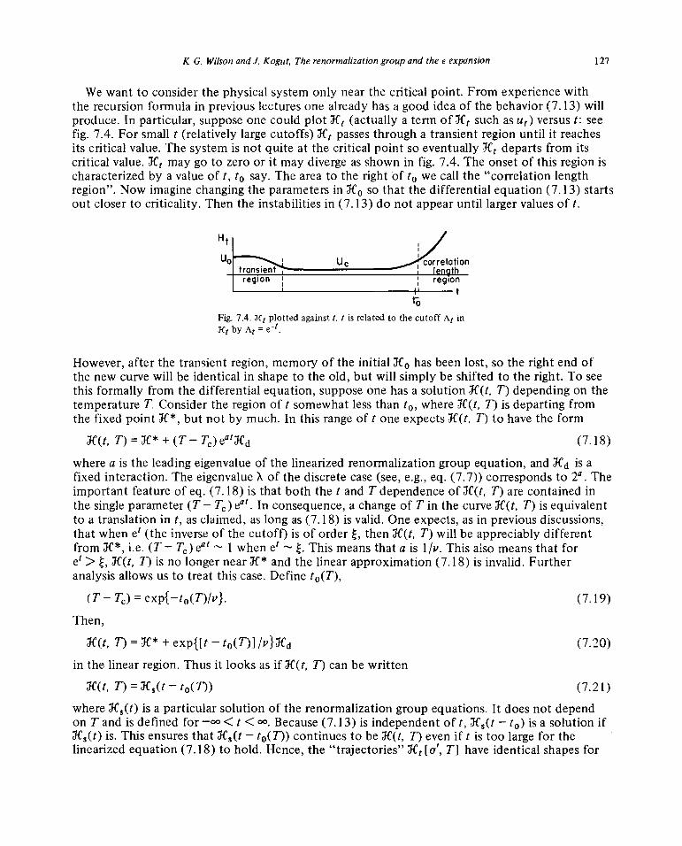
K G. WilsonandJ. Kogut, The renormalizationgroup and the � expansion 127

We want to considerthephysicalsystemonly nearthecritical point. Fromexperiencewiththe recursionformula in previouslecturesonealreadyhasa good idea of thebehavior(7.13) willproduce.In particular,supposeonecould plot ~CI.(actually aterm of X~suchasut) versus t: seefig. 7.4. For small t (relatively largecutoffs) ~ passesthrougha transientregion until it reachesits critical value. The systemis not quite at the critical point soeventually~lC~departsfrom itscritical value. ~lC~maygo to zeroor it maydivergeas shownin fig. 7.4. The onsetof this region ischaracterizedby avalueof t, t0 say. The areato the right Of t0 we call the “correlationlengthregion”. Now imaginechangingthe parametersin ~IC0so that the differentialequation(7.13) startsout closer to criticality. Thenthe instabilitiesin (7.13) do not appearuntil largervaluesof t.

~~ient~ uc ~co~onregion region

II t

toFig. 7.4. ~ctplotted against t. t is related to the cutoff At in

~t by At = et.

However,afterthe transientregion,memoryof theinitial ~1C0hasbeenlost, so the right endofthe new curvewill be identicalin shapeto the old,but will simply be shiftedto the right. To seethis formally from thedifferentialequation,supposeonehasa solution~C(t,T) dependingon thetemperatureT. Considertheregion of t somewhatlessthant0, where~fC(t,T) is departingfromthe fixed point ~ but not by much. In this rangeof t oneexpects~C(t,T) to havethe form

~IC(t,T)~lC*+(TTc)ea(~1Cd (7.18)

wherea is the leadingeigenvalueof the linearizedrenormalizationgroupequation,and~Cdis afixed interaction.The eigenvalueA of the discretecase(see,e.g.,eq. (7.7)) correspondsto 2~2.Theimportantfeatureof eq. (7. 18) is thatboth the t andT dependenceof ~W(t,T) arecontainedinthesingleparameter(T — Tc)~ In consequence,a changeof T in the curve~C(t,T) is equivalentto a translationin t, asclaimed,as longas (7. 1 8) is valid. Oneexpects,as in previousdiscussions,thatwhenet (the inverseof thecutoff) is of order ~, then~!C(t,T) will be appreciablydifferentfrom ~C*,i.e. (T — Tc)e~~t1 whenet E. Thismeansthatais 1/v. Thisalsomeansthat foret> ~, ~IC(t,T) is no longernear~ andthe linear approximation(7.18) is invalid. Furtheranalysisallowsus to treatthis case.Define t0(T),

(T—T~)= exp{—t0(T)/v}. (7.19)

Then,

T) = ~C*+ exp{[t — t0(T)] /p}~JCd (7.20)

in the linearregion.Thus it looks asif X(t, T) canbe written

~IC(t,T)=X5(t—t0(T)) (7.21)

where~W5(t)is a particularsolutionof therenormalizationgroupequations.It doesnot dependon T andis definedfor —°° < t <o°. Because(7.13) is independentoft, ~C5(t— t0) is a solutionif~C5(t)is. This ensuresthat ~C5(t— t0(T))continuesto be ~W(t,T) evenif t is too large for thelinearizedequation(7.18)to hold. Hence,the “trajectories”~JCt[a’,TI haveidenticalshapesfor

128 K. G. WilsonandJ. Kogut, The renormalizationgroup and the e expansion

differentvaluesof T, as claimed.Only for small t, for which initial transientsarepresent,is~C(t,T) not equalto ~1C5(t— t0(T)).

A furtherword aboutthe initial transientregion (small t). Therearemanypossiblechoicesfortheinput interaction~JC0,in addition to the choiceof the temperatureT. Therearemanypara-metersin ~C0if oneis completelygeneralthe entire functionsu2(q), u4(q . . . q3), etc. arevariable. Only oneparameter,typically r0 = u2(0),hasto be variedto find the critical point. Forsmall t, ~tC~obviouslywill dependon all the parametersin ~1CO.But if r0 = roc, its critical value,then~ ~ ~J(*for t —~ 00; and~* is independentof the initial parametersin ~1C0.This is because~ is a solutionof therenormalizationgroupequations,and,at leastfor the examplesdiscussedin sections4 and6, ~1C’~is completelydeterminedby the renormalizationgroupequations:thereareno free parametersin ~C’

1’so ~ cannotdependon anyof theparametersin ~JC0.

Likewisein theexamplediscussedin section4 thereis only onegrowingsolutionof thelinearizedrenormalizationgroupequation,up to a multiplicative constant.But a multiplicativeconstantcanbe absorbedinto a translationin t, so all the growingsolutionscanbe obtainedfroma singlesolution~lC5(t).~JC5(t)is definedsothat~C5(—o°)= ~(*; ~C5(t)startsoutat t = —00 at thefixed point. For largenegativet, ~C5hasthelinearized form,

~C5(t)= ~ + eth~~C (7.22)

For t > 0, X5(t) candiffer appreciablyfrom ~ but is still unique.The independenceof JC* and 7C5(t) of anyparametersin ~lC0is thebasis for universality.This

will be discussedfurtherin section 12. The solution~W5(t)is called a “renormalizedtrajectory”:seesection 12.

7.2. Scalingtheoremsfor n-spin correlation functions

Now let usreturnto the analysisof the n-spincorrelationfunction (7.15).For larget onecanreplace~ [a’, T] by ~C5[a’, t — t0(T)]. Define,

f I ) = (a~.. . 14,1 exp{.~C5[a’,r]}), q5,. . .,q~,r d ‘ ( . )

~ (q,+. . . +qn)Z(r)

Then,

r(t, T)f(etqj, . . ., e~q,~t — t0(T)) ~(d)(etqi + . . . + e~q,~)

F(q1,.. .,qn;T)= ~d(q1 +. . . +q,~) (7.24)wherewe haveexplicitly displayedthe deltafunction in the numeratorof (7.15).The deltafunctionscancelafterproducingan overall factorof e_~’t,

F(q,,. . ., q~T) = ~(t, ~n e~~tf(etqi,.. ., e~q,~t — t0(T)). (7.25)

Thisrelationholds only when:1. t is outsidethe transientregion,i.e. t large;2. etq~<1foralli~n.

Thismeansthatonemust consideronly very small valuesof qj.It is convenientto introducethe variabler = t — t0(T) andhold it fixed independentof T.

Rewrite (7.20),

F(q1,. . .~ q~T) = [~(r + t0(fl, ~jn e_~t0+ T)f(eto +

Tq1, . . ., eto + T~~ r). (7.26)

K. G. Wilson andJ. Kogut, The renormalizationgroup and the � expansion 129

This formulaaccomplishesthe following. The T dependencewas originally in the last argumentofF (asin eq. (7.24)) whereit is hard to control. Now the T dependencehasbeentransferredto theexplicit exp(t0(T)) factorswhich aremore manageable.The factorsexp(t0(T))canbe expressedin termsof thecorrelationlength ~. Considerfor examplethe definition of ~adoptedin section3:

= —d ln F(q)/dq2~q_0. (7.27)

Using eq. (7.26), oneobtains~2(flrexp{2(t0(T)+r)}dlnf(q1,r)/dq12~q,_0. (7.28)

A consequenceof this formulais thatonecanwrite

exp{to(T)} = ~(fl/E(r) (7.29)

where~(r) is a functionof r andindependentof T. It is a consequenceof this formulathat ~(r) isindependentof r also.

Finally,onemustdeterminethe dependenceof ~(t, T) on t andT. This is straightforwardgiventhe differentialequation(7.17). Overmuch of the rangeoft, ~1C~is approximately~ so considerfirst the simplerequationd ln ~/dt = VE~C*I.It is convenientto defined~as

d—d5= V[~C*] (7.30)

(d5 is a constantindependentof T andt).

A solution of the simpleequationis

~(t, T) = exp{(d —d5)t}. (7.31)

Therearetwo rangesoft for which the simplified equationis incorrect; the formula (7.31) willbe modifiedto takethis into account.First of all, fort ~t0, ~JC~is not closeto ~C*;but for thisrangeof t, ~1C~canbe replacedby ~1C~[a’,t — t0(T)]. This meansV[~C~]is a functiononly oft — t~,(T),sayv(t — t0(T)). For t ~ t0(T), v(t — t0(T)) reducesto d — d5. Taking the functionvinto account,onecanwrite

d ln ~/dt d—d5+ [v(t— t0(T)) —(d—d5)]. (7.32)

This is to be integratedwith theboundarycondition~ = 1 for t = 0. The quantity t0(T) is largefor the rangeof TnearT~of interest,andfor t ~ t0(T) the term in bracketsis negligible.Thuswhen(7.32) is integratedoneis freeto integratethe bracketedterm from t = —oo to t insteadof0 to t. Thenonehas,

ln~(t,~d—d~)t+ln~B(tto(T)) (7.33)

where

ln ~B(T) = f [v(r1) — (d —d~)Idr1. (7.34)

Onenow has,

T) = ~B(t — t0(T))exp~(d— d5)t}. (7.35)

(Note that ~B is 1 whent ~ t0(T).)Finally, thereis a correctionto this formuladueto the transientregion for small t. As long as

130 K. G. WilsonandJ. Kogut, The renormalizationgroupand the � expansion

T~ T~,the behaviorof ~1C~for small t is independentof bothT andthe final large valueof t. Inconsequenceone finds that the correct form for ln ~ is,

in ~(t, T) = (d—d5)t+ ln ~B[t to(T)] + in ~A (7.36)

where~A is independentof both t andT (providedt is largeandT Tc). The constant~A doesdependon variables(besidesT) thatappearin ~ suchas a0 in section4. Usingeqs. (7.26)and(7.36)onehas

(~(n—1)d—nd~ —

F(q1,. . .,q~,~= [~A~(r) exp~(d—d5)r}I~e~T[~ f(eT~q1/~. .

(7.37)

To obtaineq. (7.11) onedefines

d n—i —

F(qç , q~,r) = [~~(r) exp(d5r)~s]’~ [~~d~] f(eTqI1/~ . . ., ~ r). (7.38)

Then,

(7.39)

But sinceneitherF nor ~dependon r, F mustalso be independentof r; thusoneobtainseq. (7.11).A strongerresult canbe obtainedfor momentalargecomparedto 1/~but small comparedto 1.

Returnto eq. (7.15)andconsiderthe casethat t lies in the ranget ~‘ 1, t0(T) — t ~ I so that~(*~ Define,

f*(q~,.. .,q~)(Z*)’(14~.. . a~exp{~C*[aI]})/od(q~+. . .+q~). (7.40)

For tin this range~B is I; therefore

F(q1,. . .~ q~,T) = ~ exp{n(d—d5)t) ~-dt f*(etqi,. . ., ~ (7.41)Thisequationhastwo consequences.First, it hasno T dependenceon the right-handside,whichmeansonecan replaceT by Tc:

F(q1,. . .,q,~,T)[’(q1,. . .,q,~,Tc). (7.42)

The only apparentrestrictionon this equationis (7.16);sincet mustbe large,the restrictionisthat till ~ 1. However, the ~Cdterm in eq. (7.18)hasbeenneglectedin replacing.X~by ~ andthis is legitimateonly if ~‘ ~ q~lfor all Iq,l (seebelow).The secondconsequenceis ascalinglaw which will be statedfor T = Tc

F(q1,. . .,qn, Tc)5 1)d~nd5F(sq1,...,sq~,Tc) (7.43)

for an arbitraryscalefactors,providedboth Iq~lands(q~lare~l. (To prove eq. (7.43), calculateF(sq1, . . ., sq~,T~)using(7.41)with qi replacedby sqi andt replacedby t’ = t — ln s.)Thescalinglaw (7.43) is (to field theorists)a consequenceof scaleinvariancefor vacuumexpectationvaluesof a field with anomalousdimensiond5. To seethis more clearly, let [‘(x,, . . ., x,~,Tc) bethe coordinatespacemulti-spin correlationfunctions

r(xi,...,xn,Tc)= f ... f ~q,2 (7.44)

K. G. Wilson and J. Kogut, The renormalizationgroup and the � expansion 131

The scalinglaw in coordinatespaceanalogousto (7.43) is

[‘(sx1, 5X~,T~)= s—ndsF(x, . . ., Xn, Tc) (7.45)

andis valid for lx~l~ 1. In anexactlyscaleinvariant field theorytherewould be no suchrestriction;the restrictionoccursbecausethe statisticalmechanicshasa cutoff momentum(lq~I~ 1) and thereforea cutoff length ‘~1;scaleinvarianceonly occursat distanceslargecom-paredto thecutoff length. The relationof d5 to ~ (eq.(7.12)) follows from comparisonofeq. (7.45)with n = 2 with eq. (2.4) of section2.

Now the restriction ~‘ ~ lq~lfor eq. (7.42) to hold will be explained.In order to neglect~ICdin eq. (7.18) thesize of(T—Tc)e’~JCdmustbe small. One can chooset andT—Tc so that

~(T Tc)eat is small; the problemis the “size” of~ICd.~Cd,like anyinteraction,mustbe the integralof an energydensity:

= $ .Xd(x) (7.46)

andthe “size” of ~iCddependson how largea volume is importantfor the integral. The approxi-materecursionformulaprovidesan exampleof the form (7.46): within this approximation,~JCdis

~JCdx—c, JR*[c2s(x)I (7.47)

(cf. (7.2) and(7.7)).Considerthex-spaceform of the two-spincorrelationfunction for ~

F(x1) = (s(x,)s(0)exp(~ICt)). (7.48)

Thisfunctionbehavesfor very largex1like exp(—1x1lIE1) where~ is the correlationlengthforJCI.. Clearly ~ canbe ignoredonly whenlxil.c~~, and~ becomesinfinite if 1C~is replacedby~* The regionoverwhich~ICd(x) is importantfor F(x1) is expectedto be a region of size severaltimes 1x11 surroundingthepointsx1 and0, from roughlocality considerations.If lxiN~Ei, Ei isnegligible in F(x1) which suggeststhis region is smallenoughso the ~Cdterm in (7. 18) is only asmallperturbation.For lxii � E~theregion is largeenoughso~Cdis no longeraperturbation.

The generalrule in coordinatespaceis that the ~Cdterm is negligibleonly for correlationfunctionsat distancesshort comparedto the correlationlength.Thisconditiontranslatedintomomentumspacemeansall the 1q11 mustbe muchlargerthan ~. Thiswas a very cursoryargument;a morecarefulbut not rigorousanalysisgives the sameresult.

This discussionof when~JCdcanbe neglectedcanbe avoidedby assumingthatF(q,,. . ., q,~,T)hasa well-definedlimit for T-÷Tc, e.g. r(q1,. . ., q,~,T) becomesindependentof ~(T) for T—i. T~.Thenthe scalinglaw (7.43) follows directly from (7.11). Thereasonfor discussingthestrengthof~d is that this is an exampleof avery generalproblemin renormalizationgroup theory.Thegeneralproblemis this: One hasan interactionXA + °~~‘Bwhere0 is a smallparameterand~

and~C8aretwo arbitrary interactions.Underwhat circumstancescan~ICBbe neglected?Forexample,0~JCBmightbe a transientterm for larget, which hasa smallcoefficient;we havecon-sistentlyneglectedsuch terms.Accordingto the abovediscussionit shouldbe legitimate toneglect~CBif oneis calculatingspin-spincorrelationfunctionswith x~i‘= 1. However, forcorrelationfunctionsat largex, onehasto considerthe possibility that ~B is enhanceddue tolargevolume effectsandis no longera perturbation.

132 K. G. WilsonandJ. Kogut, The renormalizationgroup and the e expansion

A warning is in orderhere.Supposeonetakesa short distancecorrelationfunction anddifferentiatesit with respectto a parameterin the interaction,suchas the temperature.Forillustration let theparameterbe 0. The resultingexpressioncanbe very sensitiveto the~lCBtermevenif 0 is small. The reasonis thatafterdifferentiationonehasa newcorrelationfunctioncon-taining ~CB= f~~CB(x)integratedover all space:thenew correlationfunction is no longera shortdistancecorrelationfunction.

7.3. Slow transients and their removal for smalle

Now anotherproblemalsoneededas backgroundfor the � expansioncalculationwill beconsidered.

A problemthat ariseswhend is near4 is the slow approachof the effectiveinteractions~fC~(or~C1in the discretecase)to ~W*whenoneis atthe critical temperature.Thisslow approachcanbe illustrated usingthe simplified recursionformulaof section4. The studyof this problemis importantfor the calculationsin thenextsection.

The simplified recursionformulae(4.27)havea fixed point (r~,u*) given by (4.30).Supposetheinitial valueof a0 is closeto u~but not equalto it, and thatr0 = roc(uo). Thenthe solution(ri, a1) of the recursionformulaapproaches(r*, u*) for! -÷ 00~ The rateat which r1 andul approachr*, j4* can be determinedby solving the linearizedequationsfor r1 — r* anda1 — u~.This was donein section4. The result is thatr1 — r* and111 — u~behave as 2~for large 1, where 2E is thesmaller eigenvalueof the linearizedequation.Whene is small a1 — u~goesvery slowly to 0; for

— ~ to be very small,ci must be very large.In termsof the effectivecutoff A1 = 2~!,onemusthave� ln Al large.

This slow approachis undesirablefor the purposesof the following section.Fortunately,itcanbe avoided.If onechooses11~ = u~exactly,then141 = 14~ for all 1 andthereis no problemwith the slow approachanymore.

This is not the wholestory. The full renormalizationgrouprecursionformula involvesmanyothervañablesbesidesr1 andu~.To simplify thediscussionconsidera single irrelevantvariablew1.It is not practicalto setw0 = w~becausein practicethereare too manyirrelevantvariables.Fortunatelyit is not necessaryto put w0 = w~K.Considerinitial conditions(r0, a0, w0) nearthefixed point (r*, 11*, w*). Then thesolution (r1, 111, w1) canbe computedby settingup andsolvingthe linearizedequationsfor r1 — r*, 141 — l4~ andw1 — w’

1’. Therewill be threelinearly independentsolutionsof the linearizedequationscorrespondingto threedifferenteigenvalues.In the limite—~ 0 theseeigenvaluesare4, 1, and+(* is the largesteigenvaluefor anyirrelevant variablein thee—~ 0 limit). For e small, the third eigenvalueis still closeto ~.

The growingsolution(eigenvaluenear4) is eliminatedby choosingr0 to be its critical value

roc(uo, w0). Similarly the solutionwith eigenvaluenear1 canbe eliminatedby properchoiceofl4~ therewill be a choice~ l4oc(Wo) suchthat (r1 _r*, u~—j4* w1 — w*) involvesonly thethirdsolutionwith eigenvaluenear~. Whenw is neglectedaltogether,the “critical value”

140c is just j4*•

With w takeninto account,a0~(wo)is equalto j~* only if w0 = w~K.But for othervaluesof w0,

thereis still a choiceof 140 whichmakesthe coefficientof the slowly decreasingsolutionvanish.In fact, l4oc(Wo) turnsout to be ii~ to ordere; only in order�2 is uoc(Wo) different from ,4*~Thismighthavebeenexpectedsincethe presenceof w only changes11* itself to order�2.

In conclusion,the initial valuesof all irrelevantvariablescanbe chosenarbitrarily (typicallytheyareset equalto zero). Therewill thenbe critical valuesroc andao~suchthat fC1 + ~(* like4—1 insteadof 2~.By settingr0 = roc and~

140c, ~ becomesapproximatelyequalto ~C*aftera few iterationsregardlessof how smalle is (roc and 140c, like r* andf4*, dependon e).

K. G. Wilsonand J. Kogut, The renormalizationgroupandthe � expansion 133

8. Feynmangraphcalculationof critical exponents(eexpansion)

In this sectionwe shall discussthe calculationof critical exponentsin powersof e usingFeynmangraph techniques[1261. This approachwill be illustratedwithin thecontextofstatisticalmechanicsalthoughit will alsoserveas anintroductionto following sectionson fieldtheoryandanomalousdimensions.In particular,wewish to calculatethe behaviorof the spin-spin correlationfunctionnearthe critical temperature.Fromthe discussionof the last section(seeeq. (7.45)) oneexpectsthat

F(x) l/x2~~5 (denotedF(x, 0) in section7) (8.1)

for 1 ~x E andT Tc. The calculationof this sectionwill yield d5, the anomalousdimensionof the spin field, whenthe dimensionalityd of the physicalsystemis nearfour. Variouscriticalexponentshavealsobeencalculated.See[126, 127],andtable8.1.

Table 8.1Formulae obtained to date for critical exponentsfrom Feynman graph calculations. Seesection2 for definitions ofexponents (M = H 1/6 at T Tc defines 6). The number n is the numberof componentsof the spins; elsewherein theselectures n = 1. The constant T has been calculated to be 0.60103, approximately: seeLi 27]. The formulae for i~and ~are obtained in L127l. The other exponents are derived from scalinglaws;the scalinglawsarederivedfor the � expansionin [131]:

02(n+8)~4(n±8)’ (n+28)�2—8~~~,{n~+5On’+920n

2+3472n+480O—192(5n+22)(n+8)T}e~

3 (n+2)(2n+1) (n+2)

2 2(n + 8) � ~ + 8)’ ~2 + 8(ii+8)’ ~3~3 + 128,12 +488n + 848 —48(5n + 22)(n + 8)T}�3(n+2) (n+2) (n+2)

= + 2(n + 8) � + 4(n + 8)~(~2+ 22n + 52)e2 + —~--~jdfl~+ 44n’ + 664n2 + 2496n + 3104 —96(5n + 22)(n + 8)T}�3

6 = 3 + + 2(n ~ ~ {n2 + 14n + 60}�2 + 4(n ± 8)~{n4 + 30n’ + 276n2 + 1376n + 3168}e’ + 16(n+ 8)6 {2n6 + 96n’+ 1778n4 + 12760n~+ 50280n2 + 147136n+ 263040+ 768(n + 2)(n + 8)(5n + 22)T}�4

(n+2) (n+2) (n+2)= 2(n + 8)2 � + 8(n+8)4 (—n’ + 56n + 272)�’ + 32(n + 8)6 (—5n4 — 230n’ + 1124,12 + 17920n + 46144

— 768(5n + 22)(n + 8)T}�4

(n+2) (n+2) (n+2)

2 + 4(n+ 8) � + 8(n + 8)~(n2 + 23n + 60)�2 + 32(n + 8)’ {2n4 + 89’s’ + 1412n’+ 5904n+ 8640— 192(Sn+ 22)(n + 8)T}e3

This sectionis ratherbrief, but therearenow manyotherreferenceson the e expansion;seethe supplementallist of referencesat the endof this report.

The basicideaof the Feynmangraphcalculationis the following: For physicalsystemswith dnearfour andwith scalarcouplings4(x),the strengthaof thes4(x)interactionis of order� = 4—dat the fixed point. Therefore,it is sensibleto calculateperturbativelyin theparametera. If d = 4,onewould be dealingwith the usual Feynmangraphsof i~ scalarfield theory.Then,the Fouriertransformof F(x) becomesthepropagatorof the field theoryandhasthe form (at Tc),

F(q)ce~~~{1+a1uologq2+a2u~log

2q2 +. . .). (8.2)

134 K. G. WilsonandJ. Kogut, The renormaiizationgroup and the eexpansion

Here l1~is the bares4 coupling constantanda, are certainconstants.The field theory is cutoff

dependent;thecutoff hasbeensetequalto unity as in previouslectures.Fore~ 0 all thathappensis that morelogarithmsappearin ordere, �2, etc. Seelater in this section.To obtainusefulinformationfrom the first few termsof (8.2),we mustrestrict ourdiscussionto valuesofa

0 andq2 such that

lb log q2 I ~ 1. (8.3)

In principle one could relax (8.3) andsumthe logarithmsin (8.2) to all ordersby othertechniques.However,usingwhat we havelearnedaboutthe renormalizationgroupandcritical behavior,it willbe sufficientto studyonly the first few termsin the expansion.

At the critical temperatureonehasfrom theFouriertransformationof(8.l),

F(q) ‘~= l/q2’7 (8.4)

(i~= 2 (d5 ÷1) — d). This equationcanbe expanded,if ~ is small:

F(q) ~~{l + ~ logq +~i~2log2 q +. . .}. (8.5)

If it weresensibleto comparecoefficientsof the logarithmsin (8.2) and (8.5),we could actuallycompute7~directly. In general,matchingpowerseries(8.5) and (8.2) is not sensible.This is sobecausefor mostchoicesof 110, the powerlaw (8.4) is correctonly whenq2 is sosmall thatl1~in q2 is large,in which casethe expansion(8.2) is invalid. This tight restrictionon q2 is dueto the slow approachof ~JC

1to ~C*discussedin the previoussection.Fortunately it is possibleto choosethe parametersof the initial interactionsuchthat

eq. (8.4) is valid for a largerrangeof q2. In termsof last section’sdiscussion, one must choose

l4~ = Uoc(�) so that ~fC1settlesdown to its critical form ~ afteronly a few iterationsteps.This

meansthat (8.4) and(8.5) arevalid for all q with q ~ 1, independentlyof e. Then for small�,which meanssmall ‘io, (8.2) and(8.5) arebothvalid for q in therange,

exp(—l/u0) <<q ~ 1

andthe two equationscanbematchedorderby orderin In q2.

Now we turn to the calculationfor aoc(e) (denotedl4~(�) from now on) andi~.To do this weshallstudy the following two quantities:the four point functionaR with its externallegs set tozeromomentumfor T ~ 7~,andthepropagatorF with its externallegscarryingmomentumqfor T = T~.Then, if we definethe propagatorfor T# Tc, but q = 0 (i.e.,the susceptibility)to ber~,it follows from the scalinglaws for n-point functionsdiscussedlast time that

o r~— 2r~)/(2— ,~) (8.6)

as weshall show.A secondexpressionfor UR follows from a Feynmangraphexpansionfor aRin powersof l4~.Matching thegraph expansionwith (8.6) determinesl4~(E).Then 77 is finallyobtainedin termsof � by matchingexpansions(8.5) and(8.2).

Our first taskis to prove (8.6) from the theoremsdevelopedin the last section.The initialinteractionfor the systemwill be,

~Co~—-~- $ [q2(l +q2)2 +rolaqa...q~ $ J $ aq1aq,aq3a...q,...q2..q, (8.7)

q q1 q, ‘i,

whereq is allowedto rangefrom zeroto infinity. The kinetic energypieceof ~C0hasadditional

K. G. WilsonandJ. Kogut, The renormalizationgroup and the � expansion 135

q2 dependencewhich servesas a cutoff in placeof an upperlimit on q. (Nitpickerswill discoverthatonepowerof 1 + q2 wouldhavebeensufficient.)This form of cutoff is moreconvenientforcalculatingFeynmangraphs.It is alsoconvenientto performa “massrenormalization”on (8.7).Write

= —-i. J [q2(l +q2)2 + rI aqa..q —+ f(ro — r) Uq aq — (l4~term). (8.8)

The new term in (8.8),a self-masscorrection,is treatedas a perturbationas is the ii~ term.Sincethe r dependenceis addedandsubtractedin (8.8), it canbe chosenarbitrarily. We will chooseitsuchthat F(0)(q = 0) is preciselyr1, i.e. we demandthat [‘(0) be given as if only the first termin (8.8) werepresent;all correctionsto [‘(0) dueto theperturbationsmustvanish identically.

Define the n spin correlation function in the usualway,

(a . . . ~ exp(X0))

F(q,,. . .,qn;r) q~ n (8.9)

wherewe haveindicatedexplicitly that [‘depends on r. Thedefinition of aR will be precisely,

= F(0, 0,0, 0;r)connected/F(0,r)4 (8.10)

wherethe subscript“connected”meansthat no graphsconsistingof theproductsof 2 pointfunctionsshouldappearin (8.10).The denominatorF~(0,r) is equivalentto removingself-energyinsertionson the externallegsof all diagrams.To discoverhow UR dependsuponr we referto thescalinglaws obtainedin the last lecture. In particularfrom (7.11)we have

F(q1,.. ., q,~r) E(r) -nd5 F(q1~,. . ., qnE) (8.11)

so,

F(n zeros;r) E(r)”~— 1)dnd5 (8.12)

The propagatorthenhasthe property,

F(0;r) E~~

2d5 = E2’7. (8.13)

But, [‘(0; r) = r1 by definition, so r andE aresimply related,

r1 E2’7. (8.14)

From (8.12) the correlationfunction for four spinssatisfies,

[‘(0,0,0, 0;r) = E°’~~2’7. (8.15)

Therefore,combining (8.13)and(8.15),

11R ==E’2’~42’7/E84’7. (8.16)

In termsof r this reads

UR r~ 2n)/(2—~) (8.17)

as claimed.Our nexttaskis to obtainpowerseriesfor aR and [‘(q; r) in theparameter~ This is an

exercisein computingFeynmandiagramsin 3.99 dimensions[126, 128]. The graphscontributing

136 K. G. Wilsonand J. Kogut, The renormalizationgroup and the e expansion

to UR to orderu~~areshownin fig. 8.1 andthe graphscontributingto F(q; r) to order i4 aregivenin fig. 8.2. Beforeillustrating the calculationof a graph contributingto UR, considerthe graphsinfig. 8.2. Sincethe self-massterm in theHamiltonianis definedin order that [‘(0; r) be just thefree propagatoratq = 0 andsincethe1oop integralin the seconddiagramin fig. 8.2 generatesnoq dependence, the secondgraphis completelycancelledby the self-massterm.The final diagramfor r(q; r) doesdependon q; the self-masscorrectioncancelsthisgraphcompletelyonly for q = 0.

+ + ~ + +

Fig. 8.1. Graphscontributingto uR.

+ Q uo+ X + ~ u~ +

Fig. 8.2. Graphscontributingto r(q;r). The x refers to the r, — r term in (8.8).

As an illustrationof the calculationa Feynmangraph in 3.99dimensionsconsiderthe u~,contribution to UR. It gives

2 r d~q14°J[q2(l +q2)2 +r]2 (8.18)

The angularintegrationis simpleandproducesan unimportantconstant.Now (8.18)becomes,

2 qd_ldq

const.a0 j [q

2(1 +q2)2 +rj2 (8.19)

Theedependence of (8.19)comesfrom,

qd_1 = q3’ = q3 — eq3 log q +4 e2q3 log2 q —... . (8.20)

Considerfirst the q3 term contributingto (8.19). We areinterestedin very small valuesof r, so

the rangeof the integralr ~ q2 ~ 1 will produceasingle log r,

3d 1d2

5 [q2(l +q2)2 +r]2 $4 —logr. (8.21)

Similarly the eq3 log q term in (8.20)will producean � log2r contributionto (8.19).So, we canexpectan expansionof (8. 19) in e to havethe form,

14 {ln r + e[ln2r + In r + const.] + �2 [ln3r + . . fl (8.22)

wherea hostof numericalconstantshavebeensuppressed.The integralin this examplewasparticularlysimple. In generalwe meetnontrivial angularintegrationssuchas,

J qdl sin’~2(0). . . dq dO (8.23)

andpossiblyeventwo angularintegrations.Thesearestill well-definedfor non-integerd[126, 128].

K. G. Wilson and J. Kogut, The renormalizationgroup and the e expansion 137

Using the techniquesdiscussedhereandexercisingmorecarewith factorsof 2 andir, oneobtainsthe following expansions:

uR = u0 + 9(u~/4ir2){lnr +.!jL —-i- � ln r. . .}+.. . (8.24)

for small r, and

F(q;0)—~ {i +~}~-~lnq +. . .} (8.25)

for smallq. First observethat (8.25) lacksa u0 termsinceno graphentersthe calculationin first

order.Since[‘(q; 0) q2~’7for q small, r,i mustbe of orderu~.Now look at aR. Up to the

ln r term,

UR =u0{1+

2~lnr+. . .} (8.26)

which mustbe proportionalto r(2t~2’7). The factoru0 canbe dropped(it is aconstantof

proportionality);therefore

1 +~-~ ln r ~ r2(2’7) = 1 + [~ c ÷O(u~)Iin r +... (8.27)

andwe have

u0 ~ ~.2 � + higherorders. (8.28)

Matching(8.25)with (8.5),we find:

77e2/54. (8.29)It is interestingto observethat 54 is not asmall number,soevenchoosinge = 1 resultsin 77 ~ 0.02which is smallcomparedto unity. ri hasbeencalculatedto order�~giving 77 ~ 0.04 for � = 1. Thebestguessesfor 77 from thehigh temperatureexpansiongive 0.041—0.056[129, 1301,soourroughcalculationseemsquitereliable.The anomalousdimensionof the spin field becomes,for�= 1,

d5 =4(d—2+ti)=0.5 +0.025

from the high temperatureexpansionresult.It isd5 which hasspecialsignificanceas an anomalousdimensionin field theoryapplications.And it is interestingto notethat the correctionto themeanfield theory valuefor d5 is smallcomparedto unity.

Table 8. 1 lists theresultsof Feynmangraphcalculationsfor critical exponentsobtainedtodate.Table 8.2lists the comparisonof Feynmangraph calculationsat � = 1 with high tempera-ture seriescalculationsfor the three-dimensionalIsing model(as summarizedin [130]). Thedifferencesaretoo small to be takenseriously.

Table 8.2Comparison of high temperature results for the 3-dimensional Ising model L130l with the � expansion to order ~2, exceptto order �~for,~(table 8.1) for � = 1 and n = 1, and Landau theory.

Exponent e expansion Ising Landau

0.626 0.642 ±0.003 0.577 0.037 0.055 ±0.010 07 1.244 1.250±0.003 1.00 0.077 0.125±0.015 0p 0.340 0.312 ± 0.003 0.5

6 4.46 5.150 ±0.02 3

138 K. G. Wilsonand .1. Kogut, Therenormalizationgroup and the � expansion

9. Dimensionof tensoroperators in 4 — � dimensional space-time

In thissectionquantumfield theory in 3.99space-timedimensionsd will be discussed.Inparticular,the dimensionsof tensoroperatorsrelevantto deepinelasticscatteringwill be com-putedusingthe e expansion.(For a reviewof theoriesof deepinelasticelectronscatteringandtherelevanceof tensoroperatorssee [1321.) The theory discussedhereapproachesa free field theoryfor d -+ 4, sO it is not directly relevantto physics.The importanceof the calculationis that it givesan exampleof anomalousdimensionsin a theorywhich showsscaleinvarianceat short distances.Previously the only knownexamplewas the moretrivial Thirring model. (For referenceson theThirring modelsee [133].)

The detailsof the connectionbetweencritical phenomenaand field theorywill be discussedinthe following section.Hereweshall rely on the obviousconnectionthat the Feynmangraphsdiscussedin previouslecturesaresimilar to the (unrenormaiized)Feynmangraphsfor aØ~fieldtheory.The actualcalculationwill be setup in statisticalmechanicallanguage;the obviousanalogybetweencorrelationfunctionsof spinsandvacuumexpectationvaluesof fields will allow ustointerpretthe resultsof the calculationin termsof anomalousdimensions.

To begin,considertherulesof theFeynmangraphapproachto the� expansion.The propagatorhadthecutoff form [q2(I + q2)2 + r]1 andthe vertexwas —u

0. The massrenormalizationwasdonesuchthat the exact propagatorat momentumzerowas equalto the free propagatoratmomentumzero, namely ~ Nowconsider ç5

4 field theory.The propagatoris [k2 —m2 + ie]~’andthe vertexis iA

0. Onecanrelatethe field theoreticquantitiesm2,k2 andX

1~to thestatisticalparametersr, q

2 andu0. Comparingthepropagatorsat zeromomentum,theidentification

r~~m2 (9.1)

is clear.Consideringonly smallq2 (q2 ~ 1),

q2**—k2. (9.2)

So, positiveq2 correspondsto space-likek. Therefore,the statisticalmechanicalcalculationsapply only to vacuumexpectationvaluesof fields in the space-likeregion.It is well-known thatthe internalmomentain graphshavingspace-likeexternallegscanbe madespace-likeby a contourrotation.Therefore,theperturbationtheory rulesof previouslecturesareFeynmanrulesforspace-likemomenta.The barecouplingafter rotationof internalmomentabecomes—A

0 whichshouldbe identified with —a0. m

2 appearingin theserules is not quite the true renormalizedmassbecause the renormalizationhasbeendoneat zeromomentuminsteadof on the massshell. Sincethecutoff is fixed at 1, onemusthavesmallm (i.e. small r) in order that the physicalmassbemuchlessthanthe cutoff. No wave functionor couplingconstantrenormalizationshavebeendone.

The integrationsin thestatisticalmechanicalcasewere of the form fddqwhere d is thedimensionof space.In the field theoreticcased is the numberof spaceandtime dimensions.Thusd = — � meansonly 3 — � spacedimensionsin the field theoreticcase,whereasit means4 — �

spacedimensionsfor the statisticalmechanicscase.In this section we will calculate the dimensions of several composite operators within this

framework.Defihea vertexin configurationspaceby,

U0~(q,—q) F

2(q) ~exp{iq. x} exp{—iq. y} (s(x)s(y)7~~(O)) (9.3)

where

T0~(0) s(0) V0 V~s(0). (9.4)

K. G. WilsonandJ. Kogut, Therenormalizationgroup and the � expansion 139

F(q), the exactpropagator,appearssquaredin (9.3) in orderto removeself-energyinsertionsonthe externallegsof the vertex.The operatorT0~will be denotedgraphicallyas in fig. 9. 1. We areparticularlyinterestedin the pure tensorpieceof theoperatorT0~(asopposedto the scalarpartE~T~).Choosinga ~3picks outjust this piece.

Fig. 9.1. Diagrammatic representationof the compositeoperator T0p.

In field theoretic language T,~is a linearcombinationof the stress energy tensor andthe totalderivativeV0 ~ s

2(0).The matrix elementU0~hasbeencleverly chosensothatthe total derivative

doesnot contributeto (J0~.The reasonis that the externalmomentumcarriedby T0~is zero.Itcanbe arguedon generalgroundsthat the dimensionof the stressenergytensoris d, thedimen-sionalityof thesystem,for a scaleinvarianttheory.We will seethat this is true at leastto order�2. In real life thereareotheroperatorswhich carry internalquantumnumberssuchas isospinwhich neednot havedimensiond. To illustratethis, internal quantumnumberswill be introducedby giving san internalindex. Call the new fieldss,.The theory will be constructedto be invariantunder rotations among these fields. The interaction term in the new Hamiltonian becomes

/ u~,s~s7.Thereare two possibletensors:

T,~(O)= ~ s~(0)V0 ‘~ s~(0) (9.5a)

and, /

= s~(O)V0 V~s1(0) (i /=j). (9.Sb)

T0,,,~11(O)is a tensorwith respectto the internalrotationalsymmetryas well as to spatial rotations.CorrespondingverticesU0~(q, —q) aredefinedby substituting(s1(x)s,(y)T0~(0))or(s1(x)s1(y)T~~,(O)>into (9.3).

The analysisof thesetensorswill be donefor smallr andsmallexternalmomentaq. In orderto discussthe caseq —~0, a kinematic factorq0qp mustbe removedfrom U0~explicitly. We willcalculatethe scalarfunctionsmultiplyingq0 qp. To begin,recall severalresultsfrom the lastlecture.Scalingargumentsprovedthat the exactpropagatorat zeromomentumscalesas a powerof the correlationlength,~d 2d~Similarly, the four point functionscalesas E3d_4ds/E4d- sd~whenits externalmomentaareall setto zero.Theseresultsareeasilyunderstood.In thecaseof thepro-pagator,oneis consideringthequantityfd’~x(s(x)s(0)>. The importantvaluesof x whichcontri-buteto the integral arex E. Therefore,thed-dimensionalintegral contributesE” while eachspin field contributesa factorE~’s.Similarargumentscanbe madefor thequantity U0~(q,—q)and U0~11(q, —q) whenq is very small. If dT is the anomalousdimensionof theoperatorT0~,then

U0~(q,—q) E2d_4ds F~(q~). (9.6)

As arguedabove,U08(q,—q) is proportionalto q0qp.Therefore,for smallq, F0~is proportionalto ~ Then(9.6) becomes,

U,,,,~(q, —q) ~ (q~-~ 1). (9.7)

140 K. G. Wilson andJ. Kogut, The renormalization group and thee expansion

Eq. (9.7) canbe written in termsof r and77 usingthedefinitions d5 = -~ (d — 2 + ~1)andr~ ‘-= E~i_2ds.Then(9.7) becomes,

U0~(q,—q) —~r(dT_0’_77)R2’7)q0qp (q~~ 1). (9.8)

The critical exponent77 canbe calculatedas a seriesin eby usingthe matchingproceduredescribedin section8. The only addedingredientis the presenceof internalsymmetrywhichincreasesthenumberof graphswhich mustbe considered.The appropriategeneralizationsof(8.24)and(8.25) turnout to be,

rdI2 ~a0 ~l + 4(n + 8) lnr+. . .}, q’7 1 + 32(n + 2) (l6~2)2 lnq +..., (9.9)

wheren is the numberof possiblevalues for the internalsymmetrylabel i. And finally, u0 and77can be expressed in terms of e,

a0/16ir2 = e/8(n + 8), 77 = 32(n + 2) u~,/(l6ir2)2. (9.10)

Settingn = 1 reproduces the results of section 8.The same type of analysis will now be used to determine dimensions of tensor operators.

Considerthe diagramscontributingto the vertex functionsU0~(q,—q) and U0~~t(q,—q). To order

zero in a0 the diagramsarethoseof fig. 9.2. The possiblediagrams in order a0 and u~areshown

q, I ________,,,,,~ q, i q , I

q, I q,I q , j(b)

(a)

Fig. 9.2. (a) Zeroth ordergraphscontributing to U0p. (b) Zerothordergraphcontributing to U0p, ~,.

in figs. 9.3 and 9.4. However, the diagramsof figs. 9.3 and9.4avanish.The reasonfor this is thatq doesnot appearin the loop integrationwherethe indicesa and~3appear.Therefore,thereis nopossibleway for a factorq0qp to emergefrom the calculation.Hencethegraphmustvanishidentically. The calculationof thegraphshownin fig. 9.4bconsistsof two parts.First is thecal-culationof the integralsandsecondis countingthe numberof ways thegraph canbe constructed.

Fig. 9.3. Potentialcontributionto Uc,p of order u,,. Thisdiagram vanishes.

Oneway to calculatethe basicgraphin fig. 9.4b is to do theinternalp integrationfirst,

— 1 cl” 9 11~ ~1 j[p2(l+p2)2+rIf(p+k+q)2E1+(p+k+q)2]2+rl P.

K. G. Wilsonand.1. Kogut, The renormalizationgroupand the � expansion 141

The k integrationthenreads,

2 k E[fk+ )2] d”k (9 12)

UoJ 0 ~ [k2(1 +k2)2 +r]2 ~ q

~ktqP

(b)

Fig. 9.4. Two graphsof orderu~contributing to U0p. Graph(a) vanishes

identically but (b) doesnot.

Sinceour goal is to calculateU0~andU0~1to O(u~),the d = — � dimensionalintegralscanbereplacedby familiar four dimensionalintegrals.This is true,since(9.12) is O(u~)andthe �

dependenceof theintegralswill introduceonly higherordercorrections.Eq. (9.12) is not difficultto evaluate.The contributionto U0~in the limit q -* 0 is,

~q0qp (16~2)2 lnr. (9.13)

To do the countingonemustlook at the differentwaysthe indices i and / can run through thegraph. Fig. 9.5a,b showstwo alternativesfor U0~while fig. 9.6a, b shows two alternatives forU0~1.Associatedwith fig. 9.5ais a countingfactor4 x 4 x 2n. The factorn comesfrom the freesumover indicesof the internalloop. In fact, anygraphwith an internal1oop of indicescontri-butesa termproportionalto n. Furthermore,thereare4 ways theupperfour point vertexcould

I I

~ L(a) (b)

Fig. 9.5. Graphs (a) and (b) show two distinct ways for indices to circulate through a graphcontributing to

i~i i~~i

j~j j~j(a) (b)

Fig. 9.6. Graphs (a) and (b) depict two alternatewaysfor indices to appear in graphscontributing to t

1a~,ii

142 K. G. Wilson andJ. Kogut, The renormalizationgroup and the eexpansion

be constructed.A similar factorof 4 comesfrom thebottomvertex.Finally, thereis a factorof2 from the waysof making the loopafter the two verticesaredetermined.Similarly, the countingfactor for fig. 9.5b is 64n. The total for the two figuresis 96n. Therearealsodiagramswithoutloops(of the sort in fig. 9.6b)which contributeto U0~.Taking theseinto account,the totalcountingfactoris 96(n + 2). The countingproblemfor U0~~ involvesdifferentcombinatorics.Fig. 9.6acontributes32n (the calculationis identicalto fig. 9.5a). However,this is the only graphwith a loop contributingto

t1a~~. Fig. 9.6bshowsoneof the non-loopdiagrams.Including allthe possibilitiesproducesa countingfactorof 32(n + 6) for U

0~,~.

Collectingthe integralsandthe countingfactorsgives,

[ 96(n+2) u2~ 1U0~’=2q0q0[l 6 (162)2lnrj. (9.14)

The overall factorof 2 in theO(u~)term comesfrom the fact that the indicesaand13 couldappearon either the upperor lower lines in fig. 9.5a,b etc. Similarly,

r 32(n+6) u~ 1UO~,ZJ q0qp [1 6 (16ir2)2 lnrj. (9.15)

Eq. (9.14) is to be comparedwith the scalingresult,

~ (9.16)

Sincei~is O(u~),it canbe neglectedin thedenominatorof the exponent.Then, comparing(9.16)

with (9.14) gives,

dT = d + 77 — ~ (n + 2) u~/(167r2)2. (9.17)

Using the previousresult(9.10) for ~1it is apparentthat thesecondandthird termscancelin

(9. 1 7) leavingdT=d (9.18)

as claimed.To determinethe anomalousdimensiond(T~1)for T0~~1compare(9.15) with (9.16).

This gives

d(T11)=d+ 77 —~(n+ 6)u~/(l6ir2)2. (9.19)

Using (9.10) this becomes,

d(TiJ)=d+3(~8)2 ~ (9.20)

Choosingn = 3 (so the s, form an isospintriplet) gives,

d(T,1)=d+e2/12l. (9.21)

Since� is at mostof orderunity, the deviationof d(T,1) from d is remarkablysmall.Of course,

higherordercorrectionsto d(T,/) will changethedetailsof d(T1) — d, but the semi-quantitativeresult thatd(T,1) — d is small is expectedto still hold. The reasonthe anomalyis small is that thegraphof orderu0 (fig. 9.3) is identically zero.

The relevanceof this calculationis, of course,a matterof debate.However, it doespresentanexampleof a scaleinvariant theory in which onecanactuallycalculateanomalousdimensions.It

K. G. Wilsonand J. Kogut, The renormalizationgroup and the � expansion 143

maybe that the anomalousdimensionsthatactuallygovern the behaviorof deepinelasticscatter-ing [132, 134] arealsovery closeto canonical.(For recentperturbationtheoreticanalysesofdeepinelasticelectronscatteringseerefs. [135, 1361.)

Sinceu0 is of order�, it is clearthat u0 —~ 0 for � -* 0 which meansthereis no interactionwhend-~ 4. So this calculationcannotbe applieddirectly to real elementaryparticlephysics.The hopeis thatwhatoneseesherefor dimensiond < 4 (sayd = 3) is an indication of what a morerealistictheorywill show for d = 4.

Anomalousdimensionshavebeencomputedfor the mth rank tensoroperatorsT:

a~(0) = sj(0) V01... V0 sj(0) (9.22)

T0 . . . ami/(°) =s~(0)V01 . . . V0mS/(0) (9.23)

for evenm. Thesewill be denotedT(m) and T(m)i/, respectively.The results,to order �2, are

d(T(m)) = 2~~I~I~2 ~2 [1 _(6~ l)~’ (9.24)

d T — (n + 2) 2 — 2(n + 6) 9 25( (m)i/) - 2(n + 8)2 � ~ (n + 2)m(m + 1) ( . )

10. Connectionbetweenstatisticalmechanicsandfield theory

In section9 a brief argumentwas given that the Feynmandiagramsfor the ~ interaction(convertedto imaginarytimes,i.e., a Euclideanmetric)areidentical to the diagramsfor thepartition function of earlier lectures.To be precise,the vacuumexpectationvalueof n fields ~is proportionalto the n-spincorrelationfunction. In this lecturethe sameidentity will be estab-lished at a morefundamentallevel andwith greatercare.Greatercaremeans,for example,intro-ducinga specific (andnoncovariant)cutoff procedurefor the~ theory,andnot making useofthe Feynmanexpansion.

The connectionbetweencritical phenomenaandfield theoryhasbeenrecognizedandexploitedin diagrammaticform by Gribov andMigdal [137, 1381 andPolyakov[139—1411;a detailedcomparisonof the Feynmanpathintegralto thepartition function is given by Moore [142]. Theconnectionis alsodiscussedin a thesisby Sun [1431.Theemphasisin this sectionis on thetransfermatrix (asin [143]).

Quantumtheoryon a latticewill be a crucialpart of the discussion.In this theoryonehasdiscreteoperators/~insteadof a quantumfield operator15(x). SimpleHamiltonianson a latticehavethe form of coupledharmonicor anharmonicoscillators(seebelow).A locality requirementwill be imposed:the HamiltonianH shouldbe asum,

H~Hm (10.1)

whereHm dependsonly on operators/,, nearthe site m. Quantumfield theory reducesto a latticetheoryby useof a suitablecutoffmethod;latticetheorieswill be definedfrom statisticalmechanicsusingthe “transfermatrix” formalism (see,e.g., [1441).

The cutoff proceduresarelikely to distort the original ~ theoryevenif the original theorymakessense.In perturbationtheorytheeffectsof a largebut finite cutoff canbe removedbystandardperturbationtheoreticrenormalizationtechniques.A nonperturbativerenormalization

144 K. G. Wilson andJ. Kogut, Therenormalization groupand the � expansion

theorywill be describedin section 12. At the endof this sectiontherewill be somepreliminaryremarksestablishingthe equivalenceof an infinite cutoff in the field theoryto an infinite correla-tion lengthin the statisticalmechanics.

The latticetheoriesarenot Lorentzinvariant(or Euclideaninvariant for imaginarytimes).Lorentzinvariancehasto be recoveredin a continuumlimit. The natureof this limit is deter-mined by the renormalizationprocess.In perturbationtheoryLorentzinvarianceis restored.(Forexample,the graphsin sections13 and9 areall Euclideaninvariant.)The conditionsneededtogive Euclideaninvariancein generalarediscussedin section 12.

Thereis no trivial connectionbetweenthe Hamiltonianwhich definesthe statisticalmechanicsandthe Hamiltonianof the correspondingfield theorydefinedin this section.If the statisticalmechanicalHamiltonianis definedin a spaceof dimensiond, the field theoreticHamiltonianactsin a space of dimension d — 1. Statistical mechanical interactions are denoted by ~JC,field theoreticHamiltoniansby H. The statistical mechanical interaction ~JCis moreclosely relatedto theLagrangianof the field theory(seebelowand [142]).

The transfermatrix formalism hasbeendescribedelsewhere[144], but will be reviewedhere.(It was usedin [144] asa basisfor atransparentderivationof Onsager’ssolutionof the two-dimensionalIsing model.)Considera statisticalmechanicalmodelon a discretelattice.Thepartition function is definedto be,

Z fl(fdsm exp{_~s~_uos~))exp(K~ ~ s~~sn+~} (10.2)

wherethenotationis borrowedfrom sections3 and 4. (The sumovertis a sumoverthed axes; iis a unit vectoralongthe axis i.) The partition function (10.2) involves integrationsoverthe spinsat eachlatticesite. Insidethe exponentialsthereare termsassociatedwith individualsitesandterms which couple nearest neighbor sites. Wewill now show by construction that Z can bewritten in the form,

ZtrVN (10.3)

whereN is theextentof the lattice(assumedfinite for now) andV is the transfer-matrix,whichwill be definedbelow.To begin,onemust organizethe integrationsin (10.2). For a planelatticethespin variablesareintegratedout row by row (seefig. 10.1).(For a latticeof dimensiond, a

• S S S S S

S’m S~+i

ROW+i S S S • S S

ROW 0 S S S S S •Sm Sm+1

ROW—I S S S S S S

S S S S S S

Fig. 10.1. A two-dimensionallatticeof spins.Spinswithin eachrow are labelled with a subscript.

d— 1 dimensionalsublatticesubstitutesfor a row.) Schematically,Z will be written in the form,

Z=... f ... I ... I ... (10.4)row 1 row 0 row —1

K. G. Wilsonand J. Kogut, The renormalizationgroupand the e expansion 145

wherethe rows havebeenlabelledin fig. 10.1. Sincethe interactionin (10.2) involves onlynearestneighbors,the partition functioncanbe written moreexplicitly in the form,

Z... 5 exp{~C[row 2, row l]} 5 exp{~C[row1, row oj}f.... (10.5)row! rowO

Thereis a degreeof ambiguity in the meaningof~Cin (10.5) since terms in (10.2) which involveonly row 1, say,couldappearineitherlC[row 2, row 1] or~lC[row1, row 0]. By conventionsuch termswill be divided equallybetween~C[row 2, row 11 and X [row 1, row 01. Clearly allthe ~lC’sin (10.5) areidentical in form anddiffer only by a translation.It is convenientto labellattice siteswithin a row (sublattice)by ad— 1 dimensionalvectorm. (For atwo dimensionallatticem is a scalar.)Defining Sm(s~)to be the spinsin row 0 (row 1) (fig. 10.1),it follows from(10.2) that,

1 2 ‘2 1 4 14 1

~lC[row 1, row 0] = — ~b ~ (Sm + Sm) — ~ U0 ~ (Sm + Sm) + ~ K ~ (Sm Sm +I + Sm

5m +1) +

+K ~ ~ (10.6)m

wherethe third term includesinteractionsamongthelatticesitesin rows 0 and 1. The fourthterm givesthe interactionsbetweenrow 0 and row 1.

Let S denotethe setof spins{Sm} in a particularrow. Then~fCis a function of s and 5’. Define

V(s’, s) = exp(~W(5’, s)}. (10.7)

The function V(s’, s)definestheelementsof a matrix; matrix multiplication involves integrationover all the spins5m in S. Onecannow set up an operator-wavefunction formalism.Wavefunctionsare functions iji(s); theoperatorV acting on ~,1Igivesa wave function i4i’(s’):

= 5 V(s’, S)~(S) (10.8)

wheref5 means

11m f-~0’~dSm.

On a latticeof finite extentit is convenientto imposeperiodicboundaryconditions,whichmeansonly that, in addition to couplingrow n to row n + 1 (1 ~ n ~ N — 1, say), onecouplesrow N to row 1. In this case,the partition function is Tr( VN) as promised.

The spaceof functions i/i(s) definesa Hilbert space(providedeachrow is of finite extent;otherwiseonehasan inseparableHilbert space,which makesthe rigorously-mindedcroak).TheoperatorV is an Hermitianoperatorsince~C(s’,s) is realandsymmetric.Therefore,Vcould bechosento be a Hamiltonianof somequantummechanicalsystem.However,an acceptableHamiltonianmustsatisfythe additionalrequirementof locality. V is the exponential of sumsover the latticesites.To obtaina quantitywhich is additiveoverdistantlatticesites,theHamiltonianof the field theorywill be chosento be,

H—-~-lnV (10.9)

wherer is an arbitrarynormalizationconstant.WhenK in (10.6) is zero it is easy to show thatln V is actuallya sumoverlatticesites (in this caseV is the direct productof independentoperators,one for eachsite).Thiscanalsobe verified in perturbationtheory in K [143]. Other-wise provingthe locality of in V is a nontrivial problemwhich will not be discussedfurther.

146 K. G. Wilson andJ. Kogut, The renormalizationgroup and the � expansion

To put the definition (10.9)of H into perspective,a longdigressionwill be madeon thedefinition of the Hamiltonianand the natureof theoperatorexp(—Hr)in quantummechanicsandquantumfield theory.

In the ordinary formulationof quantummechanicstherearetwo typesof restrictionson theHamiltonian. First therearegeneralrestrictionson H; it must be Hermitian,it mustobeyspecificsymmetriesin specificcases,etc. In field theoryH mustalsobe atleast macroscopicallylocal. Thesecondtypeof restrictionis a requirementof simplicity. The CoulombHamiltoniancanbewritten explicitly in termsofjust two parameters,the electronchargeandmass.This contrastswith the setof eigenvaluesof the helium atom,for example,which areextremelycomplicatedandcannotbe written down in closed form. The Hamiltonianwould be amuch lessusefulconceptif therewereno simpleway to defineit.

Evenin caseslike nucleiwherethe exact Hamiltonianis not known,the tendencyis to inventsimple modelHamiltonians(squarewell or harmonicoscillatorpotentialmodels,for example)which reproducequalitative featuresof thephysics.

In thepresentcasethe requirementof simplicity hasbeenignored.The operatorV hasbeenrathersimply defined,but In Vis morecomplicated.For example,onecannotwrite matrixelements(s’jln VIs) in closedform. The field theoriesonenormallyinvestigates(e.g.,quantumelectrodynamicsor the i/i’ interactionof a scalarfield) havesimple Hamiltonians.At least thisisthe caseif canonicalfield theory is to be believed.Therearethreeargumentsfor beinginterestedin theorieswith lesssimpleHamiltonianssuch as the onedefinedhere.First is thatonemaybeinterestedin studyingHamiltoniansof anykind that satisfy generalprinciplessuchas locality.Thenthe advantageof consideringln Vas aHamiltonian is that all the techniquesof statisticalmechanicsareavailableto solve it. It will becomeevident in section14 thatstatisticalmechanicalmethodsare morepowerful for strongly interacting(scalar)theoriesthanany field theoreticmethods.The secondargumentis basedon the universalityprinciple which will be discussedinsection 12. Whatwill be found in section 12 is that largeclassesof interactionsareexpectedtogive the samerenormalizedfield theory,so the preciseform of theinitial interaction(simpleorcomplex)is not very important.Finally, therearecutoff procedureswhich result in the form(10.9) for.H; thesecutoff procedureswill be explainedlater in thissection.

Now considerstandardquantummechanicsandtheoperatorexp(—Hr). If onedefinesa statevector i4’(r) by,

Ii,1i(r)) = exp(—Hr)Ii/i) (10.10)

where t/i is r independent,then i/i(r) satisfiesthedifferential equation,

(10.11)

This is just the SchrOdingerequationfor imaginarytime. Supposethat the statekli(r)) hasa wavefunction i/i(x, r). Then thesolution to (10.11.)canbe written in the form,

i/i(x, r) = 5 G(x, r,x’, 0)i/i(x’, 0)dx’ (10.12)

whereG is a Green’sfunction: in abstractform,

G(x, r,x’, 0) (xlexp(—Hr)Ix’). (10.13)

K. G. WilsonandJ. Kogut, Therenormalizationgroupandthe � expansion 147

As discoveredby Dirac andFeynman(see[145] or [1461), the Green’sfunctionhasa simpleform for small r. Onecanwrite formally,

G(x, r, x’, 0) = exp L[x, ±1dr } (10.14)

whereL is the Lagrangianof the non-relativisticsystemwith the time t replacedby —ir. For a

simpletime independentpotential V, the Lagrangianfor imaginarytime reads,

L—4mx2—V(x) (10.15)

(wherex is dx/dr). For small r, x is approximately,

x = {x(r) —x(0)}/r. (10.16)

Then (10. 14) becomes for small r,

1 (x_x’)2 [V(x)+ V(x’)1~

G(x,r;x,0)~exp —~m ~ 2 (10.17)

This equation provides the definition in practice of eq. (10. 14). The proof that (10.17) gives theGreen’s function for small r is given elsewhere[145, 1461.

Eq. (10.17)showsthat exp(—Hr) is a simple operatorfor small r. If r is not smallonecanwrite,

exp(—Hr)~ exp(—Hni) exp(—Hn/i) . . . exp(—H n/i) (1 factors) (10.18)

where I is so largethat n/i is small.The operators exp(—Hn/i) aresimple,andexp(—Hn) is builtfrom them by iteration. If one computes the multiple product by matrix multiplication, one has

(xlexp(—Hn)l x’> = 5... 5 (xlexp(—Hn/i) x1 ) (x1 Iexp(—Hn/l)1x2). . . (xi Iexp(—Hrfi)Ix’).

(10.19)

This multiple integral can be written more explicitly using eq. (10.17). In the limit i-~ it definesthe Feynmanpathintegral [145, 146].

In quantum field theory there is also a path integral formalism; one must introduce a cutoffto makeit well defined.Onecan introducethecutoff in sucha way that the Hamiltoniancon-tinuesto havea simple form andlikewisefor exp(—H’r) for infinitesimal r. Alternatively,thecut-off canbe introducedsothatonly exp(—Hr) for a given finite valueof n is simple. Thiswill beexplainedbelow.Neithercutoffmethodis Lorentzinvariant; thereareof courseLorentzinvariantcutoff methodstoo. (A Euclideaninvariant cutoff was usedin sections8 and9.)

Consider the Lagrangian for a scalar field theory (in d — I space, 1 time dimension):

L =5 dd x~-~-(aØ/ar)2—-}(v~)2_.L

4~2 —A0~4} (10.20)

where 15(x) is the scalar field. As the first cutoff method, replace continuous space by a lattice ofsmall but non-zero spacing a. One uses a finite difference approximation for the gradient andreplacesthe integralby asum. Let ~ be thevalueof 15(x) at latticesite m (x = ma). Then,

L = ~ ~ ~ (acbm/at)2 — ~ (øm ÷t— øm)? — — ~ (10.21)

148 K. G. WilsonandJ. Kogut, The renormalizationgroup and thee expansion

Eq. (10.21) is the Lagrangianfor a setof coupledanharmonicoscillators,with eachøm beingthedisplacementof an oscillator. The massparameterof eachoscillatoris ~ If Fm is the momentumoperator for the oscillator at m, the Hamiltonianis,

H= ~ (2a’~~~ ~(øm+Im)2P~ad_1~+Xoa1ø~). (10.22)

The operatorexp(—Hr)for sufficiently small r is (by analogywith the non-relativisticformula(10.17)),

exp ~ (— ~— a~’(~n— ~m)2 ~ ~ [(øm +1 ~m)2 + (~‘~~

_~rah/4(~ + ~)-4ra~’X0(~ + ~)). (10.23)

Howsmall must r be for this formula to be valid? To obtaina roughestimate,considertheHamiltonian(10.22) andneglectthe cS’

1 termsandthe termscSm cSm +1 which coupledifferentlatticesites.Thenthe Hamiltonianbecomes,

H— ~ (10.24)

which is a sumof independentharmonicoscillatorswith energylevel spacing,

w =~JI~l3~2. (10.25)

Sincew is the only energyscalein H, oneexpects(10.23)to be a goodapproximationwhen~ 1, which for small enough lattice spacing a, is just r ~ a.

The expression(10.23)is rathersimilar to the formulae(10.6)and(10.7) for (s’I VIs). Tomakean explicit comparisonlet 5m be the sameas cSm exceptfor a scalefactor,

Sm ~cSm (10.26)

Then eq. (10.23) becomes

(s’Iexp(—Hr)ls) exp ~ f—~b(s~~s~)—+u~(4 +s~’1)+4K1~ (5m5m+1~5~nSn+7)

+K2Sms~}(10.27)

where

b=~ {2÷2(d_l)T÷~r)

u0 A0a”~rft4 K

1 =a”~3rft2 K

2 a~~~h/n~2. (10.28)

The requirement that r be muchlessthana means that

K1<<K2. (10.29)

Nevertheless,onecanstill defineexp(—Hn)= V to be the transfer matrix of a statistical mechanicalsystem;the resultingstatisticalmechanicalinteraction is anisotropicin space,havingcouplingK2alongoneaxis, K1 along all other axes.

K. G. Wilsonand J. Kogut, The renormalizationgroupand the � expansion 149

Thus,if oneis willing to acceptanisotropicstatisticalmechanicalinteractions,onecanhavebotha simplecutoff field theoreticHamiltonianandthe relationrH = —ln V giving 1? in terms ofa transfer matrix.

It is simpler in practiceto dealwith isotropicstatisticalmechanicalinteractions,which oneobtainsby putting n = a so that K1 = K2. Now eqs. (10.22)and(10.23)areincompatible.If oneis willing to give up the simpleexplicit form (10.22) forH onecanuseeq. (10.23)to defineH;this meansthat H = —r

1 ln V as proposedearlier (with K = K1 = K2).

In summaryonecantake the formal field theoreticexpression(analogousto (10.14)),

(cShIexp(_Hn)IcS)exp[ffd~1x{~(acS/aT)2+4(vcS)2++~cS2+A

0cS4} (10.30)

and cut this off by introducing a spatial lattice of spacing a. One then has a spatial cutoff length aanda time cutoff r. If r = a, oneobtainsan isotropictransfermatrix anda non-simpleH. If n ~ a,oneobtainsan anisotropictransfermatrix andasimpleH. Eqs. (10.28)give therelationbetweenthe field theoreticparametersj.t,,~andA

0, thecutoffa and renormalization parameter ~, and thestatistical mechanical parameters b, u0, K1 and K2. Fromnow on, only the caser = a(K1 K2 = K)will be discussed.

The next topic is to establish the connection between spin-spin correlation functions and thevacuumexpectationvaluesof thecutoff quantumfield theory.The propagatorwill be discussedexplicitly, but the resultsarevalid for anyn-field expectationvalue.The relationsH = r~’ln Vand~cSm= Sm will be assumed.The standarddefinition of the propagator,in coordinatespace,is

D(x, t) = (~ITcS(x,t)Ø(0, 0)I~> (10.31)

where I&2> is the groundstate(vacuumstate)andT is the time-ordering operator. The field cS(x, t)

is the Heisenbergfield operator~15(x,t) = exp(iHt)~(x)exp(—iHt). (10.32)

Now replacethe continuousvariablex by the latticevariablem. The result is a latticepropagator

Dm(t) definedas,Dm(t) = (~4TcSm(t)cSo(0)I~1). (10.33)

Using the latticeanalogueof(10.31),onehas,fort>0,

Dm(t) = (~Icbm exp(—iHt)cSoI~2)exp(iE0t) (10.34)

whereE0 is thegroundstateenergyof H.We needthe formulafor the spin-spincorrelationfunction in termsof the transfermatrix V

(see,e.g., [144]). A point on thestatisticalmechanicallattice is labelledby a row index n andalatticevariablem within a row. A generallatticespin is sn, m~The spin-spincorrelationfunctionis

Fn,m Z’ ~. . .f .. .5 . •~~n,m~0,0exp~C. (10.35)rown rowO )

(This is for n > 0; for n <0 the integrationsover row n androw 0 appearin reverseorder.)Supposethereare 2N+ 1 rows altogethernumbered—N to N, with periodicboundaryconditions(andN ~ n). Thenit is easyto seethat for n ~ 0,

Fn,m = Tr( VN~smV’1s

0 J~N+1) (10.36)

(notethatoneof the factorsVcouplessite N to site —N) where5m is now the Schródinger

150 K. G. Wilson andJ. Kogut, Therenormalizationgroup andthe � expansion

operator5m actingin the Hubertspaceof wave functions t,li(s) definedearlier.The tracecan berewritten,

Fn, m = Tr( V2N~_n~ Vnso)/Tr(V2~~~If~). (10.37)Assumethat the HermitianoperatorVhasa uniquelargesteigenvalue.(Statisticalmechanicalconsiderationssuggestthat this is true for T> T~(K < K~)and not true for K> Kc: see,e.g.,[144]). The largesteigenvalueof V is exp(—E

0n)whereE0 is the lowest energy eigenvalue ofH = —(in V)/n. The correspondingeigenstateof V is thegroundstate ~) of H. For largeN theoperatorVN is

V” ~ I&~~>exp(—NE0r) (&21; (10.38)

the error goes to zero exponentially in N asN —~ oo• Using this result, oneobtains(for infinite N)

rn,m (~2ISmexp(—nHn)s0(1~)exp(nE0r). (10.39)

Onecannow relateDm(t) to Fn,m.The result is (for n ~ 0)

I’n,m = ~2Dm(inT). (10.40)

The functionDm(t), starting with t> 0, can be analytically continuedinto the lower half t

plane.The reasonthis is possibleis thatH — E0 is a positive operator (by definition of E0) and

thereforeexp~—i(H—E0)t}is boundedfor Tm t <0. ThisanalyticcontinuationdefinesDm(it).Conversely,if Dm(~it)is known,Dm(t) is determinedby analyticcontinuation.

In summary the spin-spin correlation function of the statisticalmechanicaltheoryis equaltothe propagator of the latticequantumtheoryat discretevalues(nr) of the (imaginary)timevariable.

Note thatwhile the original statisticalmechanicalsystemwas definedon a lattice in theimaginarytime direction, the quantumtheoryderivedfrom thestatisticalmechanicsis definedfor a continuous real time variable. However, it is difficult to evaluate Dm (t) for anyreal valuesoft or imaginaryvaluesbetweenthe latticepointsin n. To get to valuesof t betweenthe latticepointsin practiceonehasto diagonalizeVanduseexpressionslike (10.44)below. Thereareatpresentno practicalmethodsfor diagonalizingV nearthe critical point (exceptfor the exactlysolubletwo dimensionalIsing model [144]). A studyof someeigenstatesandeigenvaluesof Vas an expansionin K is describedin [143].

To replacethe spatiallatticem by a continuum is more difficult. In the field theoreticderivationof the latticequantummechanics,a latticespacinga was introduced,so onemightexpect to recover a continuum theory by letting a -~ 0. Consider,however,thephysical(renormalized) mass PR of the field theory.If onedoesnot makea massrenormalization,(thatis, if 1.10 is heldfixed as a —~ 0) then PR will be proportional to the cutoff momentuma’ ratherthan a constant. This is the conclusion from perturbation theoretic renormalizationtheory indimensiond = 4 (for 3 <d <4, PR divergesbut lessrapidly as a -~ 0). The sameconclusionresultsfrom looking atthe statisticalmechanicsin the limit of smalla, without regardto pertur-bationtheory.As will be shownbelow, the physicalmassis (~a)~where~ is the correlationlçngthof the statisticalmechanicalsystemin unitsof the latticespacing. In dimensiond 4, ~mostlikely stays finite whena -~ 0 (see below) andhencePR behavesasa

1.To prove that

PR = l/(~a) (10.41)

one compares the long range behavior of the spin-spin correlation functionandthe propagator.

K. G. Wilson and J. Kogur, The renormalizationgroupand the � expansion 151

Considerthe spin-spincorrelationfunctionFn,m in the limit of largen, with m = 0:

x exp(—n/~) (10.42)

for n ~‘ ~, apartfrom a powerof n. Now considerthe propagatorDm(—inn) for m = 0 andn large;it is

D0(—inn)= (~ZIcS0exp(—Hnn)~0jf~)exp(E0nn). (10.43)

Writing this as asum overall eigenstatesIv) of H gives,

D0(—inr) ~ exp{—(E~—Eo)n~r}I(~ZjcSoIv)I2. (10.44)

For large n the lowestenergydominates.Becauseof the symmetry for ~15—~ —cS, thelowestenergystate that contributes is not the ground state but the first excitedstate.Accordingto conventionalwisdomthe first excitedstateis asingle particlestateat rest. (This canbe demonstratedin per-turbationtheory in K [143] but is not provengenerally.)The energydifferenceE~— E

0 for thisstateis the massPR of the particle.Therefore

D0(—inn) ~ exp(—pRnn) (10.45)

for n —~ oo• (Thesumoverv becomesan integraloverthe momentumof the singleparticlestateand results in a power of n multiplying the exponential; see [147].) Comparing eqs. (10.40),(10.42),and(10.45),oneobtainsPRT = l/~. Since we have chosen r = a, oneobtainseq. (10.41).

To seethat ~ is likely to be finite for a -+ 0, considerthestatisticalmechanicswith the para-metersgiven by (10.28),in the limit a = r —~ 0. If ~ is held fixed the parametersb, u0 andK = K1 K2 all go to zeroasa —~ 0, which is not very helpful. For finite a onecanchoose~atwill without changing~ (seebelow);with theparticularchoice

= a”2)12 (10.46)

the parameters b andK have non-zero limits for a —* 0:

b-*2d, K-÷l. (10.47)

For any a onehas,

Uo Aoa’~~~ (10.48)

so ti0 = A0 ford = 4 (ford < 4, u0 —~ 0 as a -~ 0). The reason that ~ is independentof ~ is that the

changefrom cSm to5m is only a change of variables; if ~ is changedto ~‘this doesnot change

expectationvaluesof cSm at all andthe spin-spincorrelationfunction “n, m is only changedbythe scalefactor(~I/~.)2 This doesnot change~.

Ford = 4 anda -+ 0 the parameters in the statistical mechanics are: b = 8, K = 1, u0 = A0. For

~ to be infinite, K mustbe at its critical value. If A0 = 0, K = 1 is the critical value (see section 3),and ~ is infinite. For A0 � 0, 1 is not K~in general and ~ is finite. For example, for large A0, K = 1can easily be treated by an expansion in K and is nowhere near the critical point (this is analogousto theexpansionproposedby Schiff [148]).

For d <4, U0 1S 0 at a = 0, so K = 1 is the critical point for any value of A0. However, carefulexaminationof how ~behavesasa -~ 0 shows that (ta)’ is still divergentasa —~ 0, when d is inthe range3 ‘~d<4.

This endsthe digression.The basicaim of this sectionis to constructa field theory from the statisticalmechanics.In

this case one has no a priori rules for how b, u0, and K should depend on the lattice spacing a. No

152 K. G. Wilson andJ. Kogut, The renormalizationgroup and the e expansion

suchconstantappearsin thestatisticalmechanicsbecauseonenaturallyexpresseslengthsin unitsof thelatticespacing. In field theory onehasto introducethelatticespacinga as a nontrivialparameterbecausefor a field theorist the naturalunit of lengthis the reciprocalof PR. Evenifonedoesnot set PR = 1, it is necessaryfor PR to havea finite limit whena -~0.

In preparationfor constructingthe field theory,it is logical to discussthe statisticalmechanicsin unitswith PR = 1. Theseunitscanbe usedfor any choiceof the statisticalmechanicalpara-metersb, a0, andK not at thecritical point. The latticespaci.ngin theseunits is a = l/~(b,ao, K).It is a somewhatpeculiarchangeof units sinceit dependson the parametersb, a0 andK. Workingin theseunits, PR remainsfixed no matterhow onevaries theparameters.In particular, the limita —~ 0 holdingPR fixed is obtainedby letting K —~ Kc(b, a0)whereK~(b,U~)is thecritical valueof K.

Thus it is rathertrivial to obtain a finite massPR in the limit a —* 0. What is lesstrivial is toobtaindefinite limits for the field theoreticvacuumexpectationvalues asa -~ 0. The trouble isthatonehasto know how the multi-spin correlationfunctionsbehaveas K -÷ K~.In particular,oneis interestedin vacuumexpectationvalues for distanceswhich are fixed in unitsof p1~.Afixed distancein theseunits is a distance proportional to ~ in units of the lattice spacing. Thus, ifthelong rangecorrelationfunctionshavetoo complicateda behavioras K —~ Kc, therewill benodefinite limit for thevacuumexpectationvalues as K —~ K~.In section 1 2 it will be shownthatthe continuumlimit doesexist for all vacuumexpectationvaluesif the critical behavioris deter-minedby a fixed point of the renormalizationgroup.

We concludewith two brief comments.Ford<4 the conventionallydefinedA0cS’1 theoryiseasyto renormalizein perturbationtheory;only a mild massrenormalizationis required.This isrelatedto the fact that u0 -÷ 0 asa —* 0 asdiscussedearlier.However,onecanconstructa moregeneralfield theory for d<4 startingfrom the statisticalmechanicsandholding~0 fixed (insteadof A0) asa —~ 0. The existenceof the limit in thiscaseis established(assumingtheexistenceof afixed point) in section 1 2. It is this theorythat hastensoroperatorswith theanomalousdimensionscalculatedin section9.

The second comment is this. One normally takes for grantedthat theHilbert spaceof aquantumtheoryhasa positive metric(althoughtherehasbeensomeflirting with quantumfieldtheorieswith indefinite metric by Heisenbergand others).The useof the transfermatrix formalisminsuresthat the statisticalmechanicsdefinesa lattice quantumtheorywith a positivemetric. Thisis a nontrivial result, becauseonecandefinestatisticalmechanicalmodelswhich cannotbeequivalentto quantumtheorieswith a positivemetric. A simple exampleis a Gaussianmodelwith interaction,

~ICo=fq[ro+q2]2UqU_q. (10.49)

The propagatorof this theory is l/(r0 + q2)2 which hasa doublepoleat q2 —r

0. A doublepolecannotoccurfor a quantumtheorywith positivemetric. Therefore,this theorycannotbe writtenas a latticetheoryhavinga transfermatrix. The main restrictionof the transfermatrix approachisthat thereonly be nearestneighborinteractionsbetweenrows, so that eq. (10.7) is valid. Hence,latticeapproximationsto (10.49)necessarilyinvolve secondnearestneighborinteractionsatleast.

11. Exact renormalization group equations in differential form

The purposeof this sectionis to presentan exact formulationof therenormalizationgroupindifferential form. Theseequationsarevery complicatedsotheywill not be discussedin great

K. G. Wilsonand J. Kogut, The renormalizationgroup and the e expansion 153

detail.However, the underlyingconceptswill be stressed.(Theequationsderivedherewerereportedinformally by KGW to the Irvine conference(1970);theyhavenot been publishedpreviously.)

The formal discussionof consequencesof the renormalizationgroupworksbestif onehasadifferential form of therenormalizationgrouptransformation.Also, a differential form is usefulfor the investigation of properties of the � expansion to all orders (for questions like “does itexist”; this questionhasnot beenansweredyet). A longerrangepossibility is thatone will be ableto developapproximateforms of the transformationwhich canbe integratednumerically;if so,onemightbe ableto solveproblemswhich cannotbe solvedanyother way.

In previoussectionsa discreterenormalizationgrouptransformationwas definedby integratingout the spincomponentsUq with I~I> 4. Thenonemadea changeof scalein the remaining0q (I~I<4) replacingthem by ~a’~ with ~ beinga constant.

The obviousway to constructan infinitesimal transformationis to integrateout only thosea~,with 1 — bt < ~I < 1 for öt small. This howeverturnsout to be difficult. The problemis thatnormally to ordert5t a Feynmandiagramwill haveatmostone internalmomentumin this range;however,when two internal momentaarerestrictedto be +q and—q by particular choices of theexternalmomenta(e.g.,whenp = 0 in fig. 11.1),then two internal momentacanbe simultaneouslyin the range1 — 6t < I~l< 1. This fact createsproblems.Seesupplementalref. [5] for furtherdiscussion.

~ :~.Fig. 11.1. A Feynmandiagramwhichis difficult to handlein an infinitesimalformulationof the discreterenormalizationgrouptransformation.

More philosophicallyspeakingit is desirableto avoid sharpboundariesin momentumspacebetween integrated andunintegratedspin componentsaq. The troubleis that sharpboundariesinmomentumspaceresult in non-localinteractionsin positionspacewhich onewould prefertoavoid(seesection1).

To avoid sharpboundariesa trick will be used.A smoothinterpolationprocedurebetweenintegratedandunintegratedvariableswill be introduced,called “incompleteintegration”.Thiswill permit replacingthe sharpboundaryin q spaceby a finite interval in q for whicha~is“incompletely” integrated.(Seefig. 11.2.) Thereare manywaysof realizingthe ideaof incom-pleteintegration.The particularchoicepresentedbelowhappensto havemanyuseful featuresbut

not terribly ,‘olmost

nintegroted integrated integrated comp~y

____________________ — I

(a) (b)

Fig. 11.2. (a) A sharp boundary betweenintegrated and unintegratedmomenta.(b) A smoothboundary betweenalmostcompletelyintegrated and not terribly integrated momenta.

154 K. G. WilsonandJ. Kogut, The renormalizationgroup and the � expansion

is certainly not unique. The idea will be introduced by considering an ordinary integral in placeof a functional integral.

Recall a few facts about differential equations. In particular, consider the differential equation,

a~aia ~ (11.1)

Solutions to(ll.l) can be written in termsof a Green’sfunction,

i/i(x’, t) fdx G(x’, t;x, 0)cSo(x). (11.2)

Because (11.1) is quadratic in x and a/ax, the Green’s function is known explicitly: it is,

G(x’, t;x, 0) ~2~(l —exp(—2t)) exp[—~’~~I~]. (11.3)

Eq. (11.2) providesa particularlysimple realizationof the notion of incompleteintegration.Ast —~ 0, the Green’s function becomes b(x — x’) andi/I(x’, t) becomesthe initial arbitrary function~1I0(X),

l/i(x’, 0) = i/i0(x’). (11.4)

As r becomesvery largei/i(x.’, t) becomesproportionalto the integralfi/i0(x) dx apart from theknownGaussianfunctionexp(—~

~ 5 ~0(x)dx. (11.5)

Therefore,consideredas a functionoft, l/i(x’, t) givesan interpolationbetweena completelyunintegratedfunction i/i0(x’) and its completelyintegratedform. Thus t givesa measureof howfar thevariablex hasbeenintegrated.

Considernow the functionalintegral. Sinceeachmomentumcomponentof the fieldsmustbeintegratedover, a quantityc~~(t)mustbe introducedto measurehow completelyeachcomponent0q hasbeenintegrated.A particularchoiceforc~(t)will be introducedshortly. In general,onewantsaq(t) to havethe shapedisplayedin fig. 113. Let a~denotethe spin variable for theHamiltonian~iC~before the momentumhasbeenrescaledfrom the original momentumscale.The

-- f~3,— _———t~a

aq(t)

----Iq

Fig. 11.3. A choiceof the function aq(t) whichmeasures(asa functionof t) how completelyeachcomponent°qhasbeen integrated.

K. G. Wilsonand J. Kogut, The renormalizationgroupand the e expansion 155

spin variableafter thescalechangewill bedenoteda~7.The functionalanaloguesof (11.1)and(11.2)become,

= + ~ exp~X~[a”]}, (11.6)

exp{~Ct[a”]} c fexp{_4 5 (u~ üq exp{—a~7(t)})(a~qU.q exP{_c1~l(t)})}{~[]}q 1 —exp{—2a~(t)} (11.7)

The constantc is unimportantsinceoneonly computesratiosof expectationvaluesinvolvingexp(~C~).G~qandU...q appearin the right-handside of(11.7) in orderthat .Xt[a] conservesmomentum.A functionaldifferentialequationfor JC~[a”] follows straightforwardlyfrom (11.6)

= 5 ac~(t){~~r ~ + o2~Jc~+ ~ + const.}. (11.8)

at q at öcrq t5fL.q tSfJq ~U..q

The “const.” is a a” independentterm which canbeignored.Now a usefulctq(t) mustbe chosen.This function shouldhavethe propertythat it separates

smallq from largeq. A good choiceturns out to be,

aq(t) = q2(e2t— 1) + p(t), p(0) = 0. (11.9)

The purposeof the functionp(t) is to allow a normalizationconditionto be imposedon the

kinetic term in ~ say

t~4 Sql2a~alq+ (11.10)

(in termsof a~’which will be definedshortly).Clearly p(t) servesthe samepurposethat ~ did inthediscretescalechangesof earlierchapters(see,e.g.eq. (3.33)).Somesuch normalizationconditionturnsout to be essentialif critical behavioris to be describedby a fixed point. Imposingthis normalizationconditionon ~fC~for all t resultsin an equationfor p(t).

The final stepin constructingthe renormalizationgrouptransformationis the changeof scale,i.e. ~IC~shouldbe written in termsof a momentumvariableq’ whoserangeis effectively0< Iq’I < 1. From (11.7)and (11.9) it is clearthat the effectivecutoff on q is e_t, so the rescaledmomentumq’ shouldbe q’ = qet. Also, the rescaledspin variablea~’mustbe introduced.It willbe definedto be

a~,’—exp(—dt/2)a,’. (11.11)

The scalefactor is determinedby the requirementthat the differential renormalizationgrouptransformationwe will derivemustbe independentof t. (It is easilyseenfrom (11.8) thatonecannotmakearbitrarychangesof normalizationof a~without fouling up the equation.)

The functionaldifferentialequationmustnow be rewrittenwith c.sq’ replacing0q• The timederivativea~C~/atin (11.8) is for a fixed functiona~.This mustbe replacedby a derivativeforfixed 4. The relationbetweenthe two timederivativesis

= + 1 ~ (1112)at ~ at ~, ‘, dt ,,‘ ~

156 K. G. Wilson andJ. Kogut, The renormalizationgroupand theeexpansion

The derivativeda~’/dtI0”follows from (11.11),

da~ Iddt ~. = ~ (11.13)

so(11.8)becomes,

= ‘r(g +q’ .~q)a~,];~ct+5 ~ C~ ~ ~—j~—+ ,, ,,q at 6a~50_q öuqba_q q ~ij. (11.14)at~

0 ,L2

But, from(11.9)

aa,~/at= 2q2e2t + dp/dt = 2q’2 + dp/dt. (11.15)

Finally, (11.11) andpropertiesof functionalderivativesimply,‘p

= exp(dt/2) ö.JC1/~a~’. (11.16)

Substituting(11.15)and(11.16) into (11.14)gives thedesiredrenormalizationgroupdifferentialequation,

a~lC~ fld , ______

at J aq’ + q Vq’a~’) ~ + 5(~+ 2q’~)~ + _______ ,öfJq q’ dt ~aq ~ ~aq’6a_q’ ‘

(11.17)

This is a functionaldifferentialequation.It canbe reducedto ordinarypartial differentialequationsby expanding~ in powersof a: write (theprimeson a andq are omitted),

~Ct[a] —~fu2(q,t)aqa_q ~i I I 5u4(q,qi,q2,q3,t)aqaqaq2aq, —. . . (11.18)

4! ~‘ ‘-‘q qq,q2(whereq3 = —q — q1 — q2 to conservemomentum).A constantindependentof a hasbeenomitted.The equationsfor u2, u4, anda6 are

au2t) {—q V + 2 + 2q2) [1 u2(q t)]} U2(q, t) + 5 (~+2q~)u4(q,—q, q1, —q1, t)\dt\dt

~

x [I — 2u2(q3,t)]} u4(q,. . ., q~,t) + + 2q~)a6(q, q1, q2, q3, q4, —q4, t)

q4

Idp~(q. . . q5, t) = {_2d — q . + + 2q2) [1 — 2u2(q, t)] —. . . — q5 . Vq, +(~+ 2q~)

x [1 — 2u2(q5, t)]}u6(q,.. ., q5, t) — 2[~+ 2(q +q1 +q2)2]

X U4(q, q5, q2, q3 + q4 + q5, t) U4(q3, q4, q5, q + q1 + q2, t) —(9 permutations)

+ f(~~+2q~)u8(q,. - .,q5,q6,—q6,t). (11.19)\ dt

K. G. WilsonandJ. Kogut, The renormalizationgroup andthe � expansion 157

The “9 permutations”in the equationfor u6 meansthe 9 inequivalentpermutationsof(q1, . . ., q5) in the u4 X U4 term.

So far, no equationhasbeengiven for dp/dt. The normalizationcondition(11.10)meansthatif u2(q,t) is expandedin powersof q

2:

u2(q, t) = U2A(t) + a2B(t)q

2 + . . . (11.20)

thenu2B(t)= 1 independentoft.This meansdU

2B(t)/dt is 0, which resultsin an equationfor dp/dt.Write u4 as an expansioninpowersof q:

u4(q, —q, q1, —q1, t) = U4A(q1, t) + q q1u4~(q1, t) + q2U

4c(qi, t) + (q . qi)2U

4D(q1, t) +.

(11.21)

(This expansionassumesrotationalsymmetry.)Then theequationdeterminingdp/dt is,

02U2B~(t)[12U2A(t)]_2u2B+4U2A[1_u2A}+f[~(r)+2q~]

x[a4~(q1,t)+d~q~u4~(q1,t)].(11.22)

Howeverthe readeris warnedthat the simplenormalizationconditiona2B(t) = 1 for all I cannotalwaysbe realized;onemustbe preparedto allow U2B(t) to be anotherconstantor perhapst

dependent.Seethe Appendix for an exampleof the solutionof the renormalizationgroupequationsandadeterminationof dp/dt.

We know how to obtainspin-spincorrelationfunctionsgiven ~C0,but it is desirableto be ableto obtainthemwhengiven ~ To do this first considerthe generatingfunctional originally givenin termsof ~C0andthenrewrite it in termsof~C~.The analogousproblemfor onevariable,x, willbe sketchedto begin.The l/10(x) of eq. (11.2) is analogousto exp(.~C0[a])soconstructthegeneratingfunctional:

Z(j) = 5 i/.’0(x’) exp(jx’) dx’. (11.23)

A straightforwardcalculationshowsthat this is equivalentto

Z(j) = 5 5 exp(/x’et — 12(e2t — 1)) G(x’, t; x, 0) p

0(x)dx’ dx (11.24)

for any t. (To prove this oneperformsthe x’ integrationusingthe explicit form (11.3) for theGreen’sfunction.) Reversingtheorderof integrationgives

Z(j) 5 ~(x1,t)exp{Jx’et_1~2 ~}dx’. (11.25)

Now considerthe generatingfunctionalof actualinterest

ZU)1 exP~f/(q)aq+~Co}. (11.26)

158 K. G. WilsonandJ. Kogut, Therenormalizationgroup and the � expansion

In termsof~Ctand q”, onehasin analogyto (11.25),

Z(j)-~J exp{fJ(q)a~q exp~aq(t)} -4 5 j(q)j(-q)[exp{2~q(t)}- 11 +~c~} (11.27)

andconvertingto a’ gives

Z(j) = j exp~5 e~tI2e~t)j(q’e_t)aqexp[(q’)2 — (q’)2 e_2t1

4 5 j(q1et)j(_q’et)e~t[exp(2q’2 — 2q12e2t+ 2p(t)) — 1] + ~C~[a’]}. (11.28)

This is a rathercomplicatedformula. Accordingto the generalprinciplesof the renormalizationgroupapproach,the only change.in calculatingcorrelationfunctionsfrom ~JC~as opposedto ~W

0shouldbe a scalechange;namely,a_q shouldbereplacedby ~ta~q’with q’ = qet. In otherwords,oneshouldwrite

5 j(q)a_~= e~t~tI i(qPet)a~q = f j(q’, t)a~q’ (11.29)

with

j(q’, t) = e~t~~j(qPet). (11.30)

Supposeonedefines

= e°’~2ep(t), (11.31)

then(11.28.)becomes(droppingprimes for convenience),

Z(j) = J exp { 5 j(q, t)aq exp[q2 _q2 e2t1 —~ 5 j(q, t)j(—q, t) [exp(2q

2 — 2q2e2t)— e2P(t)]a q q +~Ct[u]}. (11.32)

This formula for computingZ(j) is morecomplicatedthanexpectedfrom generalprinciples.However, it will not affect the generalrenormalizationgroupanalysis:For larget andq of order 1,the e_2tande2P(t) termscanbe neglected(neglectinge2P(t) assumesthatp(t) -+ °° as t —~ °°; thisis true of examplesthat havebeenstudiedto date).ThenZ(j) dependson t only throughj(q, t)

andthe t dependenceof ~C1..This is the crucial fact neededfor a generaldiscussionof conse-

quencesof therenormalizationgroup.It is remarkablethatonecanwrite an exactyet completelyexplicit form for a~c~/at(eq.

(11.1 7)). Previouslyall formulationsof the renormalizationgrouphaveinvolved perturbationtheory in an essentialway (asin theGell-Mann---Low formulationor the graphicalformulationofsections4 and 5) or elseinvolve incalculablefunctions(the Kadanoffapproach).Eq. (11.17) canbe nastyto work with, but in the long run it or similarequationswill probablybe the basis formostwork on the renormalizationgroup.

For future referencethe form of Z(j) for large t is,

Z(j) = j exp {f j(q, t)a_~exp(q2)-4 5 /(q, t)j(-q, t) exp(2q2)+ ~Ct[a]}. (11.33)

K. G. Wilsonand J. Kogut, The renormalizationgroup and the � expansion 159

This is the formulathat is usedfor ~JC1.[a] neara fixed point ~C’~or on a renormalizedtrajectoryleaving~C*.

Note thatactualcorrelationfunctionsalwaysinvolve a denominatorZ’ so the generatingfunctionalof practicalinterestis Z(j)/Z(0). This is fortunatebecausetheconstanttermin JC~wasneglectedin deriving the differentialequation(11.1 7).

Thereis anotheruseful formulafor the generatingfunctionalZ(j) (moreprecisely,Z(j)/Z(0)).The formulais the following. Definea particularfunctiona~(q)to be

a(q) =j(qet) exp~/3q(t) dt/2} (11.34)

where

!3q(t) = q2(1 — e_2t)+ p(t) = ~q exp(_t)(t). (11.35)

Then,

Z(j) ~ exp{~Ct[a~]+4 5 a(q)a(-q)[l + exp{-2~q(t)}1). (11.36)

This formulais demonstratedas follows. First write (11.7) in termsof a~(q),thenlet t -~ oo anduse the definition (11 .26) to identify Z(j). To begin relate the unscaled variable a~’to the scaledvariablea~,

a~’(q)= exp(dt/2)a~(qet) j(q) exp{c~(r)}. (11.37)

Substitutionof a~(q)for a~in (11.7)gives,

{~[ ]l — I —~ I j(q)j(—q) exp (2c~(t~l

exp a~~ — c exp 2 — exp{—2cz.~(t)ILI

x 5 expt J ~ —~J ~ +~fC~[a]}. (11.38)

In the limit t —~ 0O~(11.38)canbe rewritten,

lim.exP{~Ct[afl +~ 5 a~(q)a~(-q)[l +exp{-213q(t))]} c 5 exp~Ji(q)aq +XoEa]}.q a q (11.39)

Fromits definition (11.26),Z(j) canbe recognized as (11.39). The advantage of(1 1.36) is that itavoids the explicit calculation of functional integrals; it is only necessaryto solve the functionaldifferentialequationfor W

1..

12.

12.1. Topology of the renormalizationgroup transformation(fixedpoints, trajectories,andsubspaces)

Underlying the detailed calculations andanalysesof the renormalizationgroup approachdescribedin previoussectionsare somesimpletopologicalideas.Fixed points, for example,havealreadybeenemphasized.In this sectiontopologicalideaswill be consideredat length.They will

160 K. G. Wilson and J. Kogut, Therenormalizationgroupand thee expansion

be discussedin simplebut abstractform without referenceto specific formsof the renormaliza-tion group transformation.A few generalassumptionswill be madeconcerningthe effectiveinteractionsgeneratedby the renormalizationgroup.Theseassumptionsaretrue of solutions(exactor approximate)obtainedto date,but havenot beenprovenin general.Simple formsofthe topologywill be consideredto illustratethe ideas.In actualexamplesthe topologygetsmorecomplicated(e.g. manydifferent fixed pointscanoccur)but onecanhandlecomplicationsoncethe ideashavebeenmastered.

Fixed pointswerediscussedin the originalpaperof Gell-MannandLow [149] (seealso [150]).The needfor a full topologicaldiscussionaroseonly whenthe renormalizationgrouptransforma-tion was definedto transformmanycouplingconstantsratherthanjust one. A completetopologicalanalysiswas first given for a simplified fixed sourcemodel [151]; muchof the inspiration for thissectioncomesfrom [151]. Wegner[152] hasgiven an extensivediscussionof solutionsof therenormalizationgroupneara fixed point,which overlapsand considerablyextendsthelast partof this section.

SpacesandsubspacesA renormalizationgrouptransformationis a transformationU on aspaceof cutoff interactions

S. In the previouslecturean exampleof an infinitesimal transformationU hasbeengiven. Therenormalizationgroupequationis

aK~/at=U[~JC~]. (12.1)

The interactions~ come from the spaceS.The interactionsin S are givenin dimensionlessform with momentagiven in unitsof thecut-

off. Oneis always free to takeanyinteraction~CE Sand changethecutoff by making achangeof units. The cutoff can consistof an upperboundon all momentaq imposedeitherdirectly orthroughthe introductionof alattice(cf. sections3 and 10). The cutoff is necessarybecausetherenormalizationgrouptransformationU is definedto integrateout the momentajust belowthecutoff andthat is a meaninglessoperationif the cutoff is infinite. In the caseof theexactrenor-malizationgroupequationsof section 11,a strict upperboundon q is not necessary,but it isdifficult to integratethe equationsif the non-Gaussiantermsin ~lC0are not cutoff for momentaq ~ 1. In the renormalizationgroupapproachanuncutoff field theoryhasto be obtainedasthelimit of cutoff theories.(This is independentof whetheroneis calculatingin perturbationtheoryor not.)

The coordinatesinSarethe free parametersin an arbitraryinteractionX E S. In the simpleexamplesconsideredin previouslectures,r andawere coordinatesin S. To discussthe exactrenormalizationgroupequations,an arbitraryinteractionin ~Cis definedin termsof an infinitesetof arbitrary functionsu2(q),u4(q,q1, q2, q3), etc. This meansS is an infinite dimensionalspace.

A solution~ of the renormalizationgroup, as a function of t, providesa setof interactionsall of which describethesamephysicalsystem.Howeveronemustmakea t-dependentchangeofscalewhenrelating~iC~to the physics.Onecanfirst of all makea scalechangewhengoing from~C0to the physicsso that the physicshasa cutoff momentumA0 ~ 1. This is a scalechangewithno restrictions:A0 can be chosenat will. Given A0, the scalechangewhich relates~IC1to thephysicsis fixed, namelythecutoff momentumof~C~in physicalunitsmustbe e_tAo. (See,e.g.,section7.)

Let the physicalsystemhavea correlationlength ~ in physicalunits (cm or MeV~,say). Thismustbe independentof which interactionX1. (i.e. which valueoft) is usedto describethephysics.

K. G. Wilsonand J. Kogut, Therenormalizationgroup and the � expansion 161

Let ~ be the correlationlengthof ~ in dimensionlessunits. Thenthe scalechangesdefinedaboveimply that

= ~ (12.2)

This in particularmeansthat ~ satisfies

~t ~ (12.3)

for a solution~JC~of eq. (12.1).The interaction~C1.rescaledto physicalunits hasan artificially smallcutoff e_tAo comparedto

the true cutoff A0 of the physicalsystem.This is by construction;the highermomentain ~JC0havebeenremovedby integration.The artificially low cutoff meansthat the interactionsin 1C~areartificially of long range.The interactionsin the rescaled~C1,will havea rangeof orderet/Ao,at least.The initial interaction~C0,rescaled,hasinteractionsonly of range1/A0 unlessonedeliberatelyaddslongerrangeinteractions.

In practicea “short range” termin ~C0,before rescaling,is for examplef~f~exp~—(x y)2} x

s(x)s(y)while examplesof “long range” interactionswould bef~f~exp{—0.000l(x —y)2} s(x)s(y)(which hasalong but finite range)or f~f~Ix —yj~s(x)s(y)(which hasinfinite range).

The spaceS will be restrictedto interactionsof short rangein dimensionlessunits. Thereareseveralreasonsfor this. Oneis a practicalone: the approximationschemesof previouslecturesconsideredso far assun-’ethat~ hasonly simpleshort rangeinteractions.A more fundamentalreasonis that the qualitativeideasaboutcritical behavior(like universality)are knownto be falseif long rangeinteractionsarepermitted.(See,e.g., [1531.) It will alsobe crucial to the renormali-zationtheorydescribedlaterthatS haveonly short rangeterms.

The spaceS mustbe largeenoughsothat for anyinteraction~ E 5, all the effectiveinter-actions~ generatedfrom ~lC

0lie in S. Thusonemust verify, for example,that the interactions~JCtareall of short range(beforerescaling).Thereis unfortunatelyno certaintythatthis is thecasein general.It is true of examplessolvedso far. (Note howeverthat an incorrectchoiceofp(t) in the equationsof section 11 can leadto long rangeinteractions:seethe Appendix.) Inapproximateformulationsof the renormalizationgroup (e.g.,the approximaterecursionformulaof section6) onecanreplaceS by a subspaceof S but onemustmakesurethat the approximatetransformationtransformsthe subspaceinto itself.

Thereare four typesof subspacesor “surfaces”in S which should be defined.First the elementsof S canbe separatedaccordingto their correlationlengths.Thus,onedefinessurfacesconsistingof all interactions~lCE S with given dimensionlesscorrelationlength~. Of specialinterestwill bethe “critical surface”with ~ = 00 denotedSe,. Fig. 12.1 showsa possiblesetof surfacesof fixed ~in a spaceparametrizedby r andu only.

r— e

Fig. 12.1. Linescharacterizedby fixed valuesof thecorrelation length ~. The line labelled I = is the“critical surface” Sc.

162 K. G. Wilsonand J. Kogut, The renormalizationgroup and the � expansion

Secondly,thereis a surfaceof simple interactionsto be called the“canonical surface”.Thissurfaceconsistsof the setof initial interactions~ for a given systemor model. For example,the canonicalsurfacemight consistof the interactions(4.2) with r and u as the only freeparameters.

Thirdly, therearesurfacesof definitesymmetry.Forexample,in order to allow for interactionson a lattice,S includesnon-rotationallyinvariant interactions.(Interactionson a three-dimensionalcubic lattice havecubicsymmetrybut not full rotationalsymmetry.)Thentherewill be a subspaceSR of interactionswhich arerotationallyinvariant.

Finally thereare thesubspaceS(t) generatedby applying U to the spaceS itself. This meansthe following. Supposeonestartswith a spaceS as illustrated in fig. 12.2 and an infinitesimal

boundary S

Sboundary: S (t)

boundary S(2)

Fig. 12.2. NestedsubspacesS(t). in this example thesubspaceS(=) is onedimensional.

transformationU definedon S. The spaceS(öt) with t5t infinitesimalis definedas theset of points

~iC‘ suchthat,

(12.4)

where~JCis somepoint in S. Onethenobtainsthe spaceS(2t~t)by applyingU to the spaceS(~t):S(28t)consistsof all interactions~C’of the form (12.2)where~1Cis somepoint in S(6t). ByinductiononecandefineS(t) for any t. In otherwords,if onesolvestherenormalizationgroupequationsto obtain~ from ~C0,then5(t) is thespaceof all interactions~ generatedfrom allpossibleinitial interactions~o containedin S.

By assumptionthe effectiveinteractions~JC~lie in S soS(t) is asubspaceof S.The subspacesS(t) arenested:S(t + t ) C S(t) for anypositive t andt. The reasonis simple:

S(t+ r’) is obtainedby integratingthe transformationU througha time t + t’, starting from allpointsin S. This is equivalentto integratingU througha time t starting from all pointsin S(t’).Since5(t’) is containedin 5, onegetsa largerspaceby starting from all pointsin S insteadofS(t’): hence,S(t + t’) C S(t).

The spacesS(t)for finite t havethe samedimensionalityasSitself. However,the spaceS(c0)

(obtainedas the limit of S(t) fort —~ oc) canbe smaller.A basicideaof the renormalizationgroupapproachis that S(oo) is a surfaceof manylessdimensionsthanS. For illustration the surface5(oc) in fig. 12.2 is a singlecurveC. Thereasonthat S(oc) is expectedto be muchsmallerthanSis the following: ~JC~(for larget) describesa physicalsystemwith forcesof amuch shorterrangethanthe rangeof interactionsin ~ itself (asshownearlier). It is unlikely thatan arbitraryinter-actionX in S hasthis property;thusS(t) for larget shouldbe only asmall subsetof S.

A differentialequationlike (12. 1) canbe integratedbackwardsin t aswell as forwards.

K. G. Wilson andJ. Kogut, The renormalizationgroup and the � expansion 163

Suppose~lCis in S but not in S(t). Thenthe interaction~ generatedby integratingbackwardscannotlie inS. If~W~is not inS, the reasonis likely to be that ~ haslong rangeinteractionson a dimensionlessscale.In fact, alonga randomtrajectoryintegratedbackwardsonewouldreasonablyexpectall the interactions~JC~to havethe samerangein physicalunits. If this is thecasethe rangeof interactionmustgrow like et in dimensionlessunits for the interactions.X~.Hence,for larget, X...~will generallylie outsideS.

Trajectoriesandfixed pointsThe renormalizationgroupequation(12.1)definestrajectoriesin thespaceS. On a trajectory,= e_t~ Thus,if the initial interaction JC~,hasa finite correlationlength~ thenthe trajectory

passesthroughall the surfacesof fixed ~‘ with ~‘ < ~ This is illustratedby curveA in fig. 12.3a.If the initial interaction~JC0hasan infinite ~o, then the trajectorylies entirelyon the criticalsurfaceSc (curve B in fig. 12.3a).

A (translated)A ~1(t~0)

~2(t~—2n2)

B - (b)

(a)Fig. 12.3. (a) Two renormalization group trajectories A and B. Curve A begins at ~ = 2 andcrosseslines of smaller~. Curve B beginson the critical surface(I = oo) and staysthere. (b) Trajectory A translated so that I, = I.

Sincethe renormalizationgroup transformationis independentoft, it is possibleto translate

trajectoriesin the variablet (asalreadyseenin section7). The only effect of a translation,

(12.5)

is that the translatedtrajectorybeginsat t0 insteadof t = 0. Onecanusethe freedomof trans-lation in t to specifya normalizationconditionon ~ say~o= 1. Then,~ = e_t. With thisnormalizationthe surfacesof equal~becomesurfacesof equalt for translatedtrajectories(fig. 12.3b).

A fixed point is an interaction~C”satisfyingU[~JC*] = 0. A fixed point is a trivial trajectory:= ~ for all t solves(12.1). A fixed point musthavea correlationlength E* = 0 or =

(sinceifX~= ~ then~ = ~‘, but, beinga solutionofeq. (12.1)means~ = e_t~

0= e_t~*).In orderto illustratethetopologicalideas,we will now developthe simplestform the topology

cantake.Therearemanywaysin which the topologycanbe morecomplicatedthandescribedbelow,but complicationscanbe understoodoncethe simplestpicturehasbeengrasped.

Assumethereareonly two fixed points,onewith ~ 0, onewith ~* = oo~Thesefixed pointsaredenotedP0 andP,~.in fig. 12.4. The fixed point Pc,, will be assumedto havethe samepropertiesas the fixed point (r*, a*) of section4.

The simplestbehavioronecan obtain for a trajectoryin the limit t -~ oo is that it approachesafixed point. This is not theonly behaviorpossiblein principle,but it is the only limiting behaviorseenin previoussectionsandwill beassumedhere.Otherpossibilitiesarediscussedin [150] and[154]. If all trajectoriesapproacha fixed point, thenthe trajectorieswith finite ~ approachP0for t —~ 00 (e.g.,curveA in fig. 12.4)andthe trajectorieson the critical surfaceapproachP0,~(curveB, fig. 12.4).

164 K. G. Wilsonand.1. Kogut, Therenormalizationgroupand the � expansion

Fig. 12.4. Simple topology:the spaceS hastwofixed pointsP

0 andP.,.,. P.,,, lies on thecriticalsurfaceandhas~ =. P0 has I = 0. CurveBrunsinto P,.,, and A runs into P0.

Thereis a simpleanalogyin classicalphysicswhich providesan exampleof thetopology being

discussed[155]. Imaginea ball rolling on a hill accordingto theequationof motion

dx/dt VV(x) (12.6)

wherex = (x, y) arethe horizontalcoordinatesof theball andV(x) is theelevationof the hill atthepoint x. (Thisequationis a simplification of Newton’slaw in that velocity (dx/dt) replacesmasstimesacceleration.)An exampleof a contourmapof Vis shownin fig. 12.5. It is assumedthat V(x) is analyticmx. The equationof motion is an exampleof(l2.l); a fixed point is astationarypoint of V. Two fixed pointsareshownin fig. 12.5;P0 is anabsoluteminimumandP0,, is a saddlepoint. If the ball is placedanywhereto thewestof the ridgeline R, the ball rollsto thebottom of the hill (P0)andstops(the curveA in fig. 12.5 is an exampleof atrajectoryofthe ball). If the ball is placedexactly on the ridge line R, it rolls down to thesaddlepoint P,., andstops(curve E, fig. 12.5). The ridge line R is analogousto the critical surfacefor therenormaliza-tion group equation(12.1).

Fig. 12.5. Contourmaprealizingthetopology offig. 12.4. P.,., is a saddle-pointon theridge R andP0is thebottomof thegully G. PathD showsthecourseof a ball initially neartheridge line, spendingagreatdealof time nearthe saddlepoint P.,,,andeventuallyrolling downthegully G and stoppingat the bottomP0.

It is interestingto studythe trajectoryof theball whenit is placedinfinitesimally closeto theridge line R. Thenit rolls down closeto the ridge line almostto the saddlepoint. This is illustrated

K. G. WilsonandJ. Kogut, The renormalizationgroup and the � expansion 165

by the curveD in fig. 12.5. Nearthe saddlepoint the ball veersawayfrom the ridgeline androllsdown the gully G. Nearthe saddlepoint the ball rolls very slowly becausethe terrainis almostflat.

Now let the initial locationof the ball approachthe ridge R. In thislimit the curve D approachesalimiting curveE. The curveE hastwo parts;onepart is asectionof theridge line R. The otherpart is the line G definingthebottomof the gully. The gully line G is also the trajectoryof a ballwhich startsinfinitesimally closeto P,.,.

Consideragainthe simpleexampleof the renormalizationgroupwith the two fixed points(fig. 12.4). Considera trajectorywhich beginsinfinitesimally closeto the critical surface(curve Din fig. 12.6).Assumethe analogyto the classicalequationof motion is valid. Then D hastwoparts;onepart is essentiallythe trajectory E going to the fixed point P,,.The secondpart is atrajectoryG connectingthe two fixed points.(Theapproximationof replacingD by G isequivalentto the approximation(4.41)of section4. A changein tin the currentlectureisequivalent to changing n in (4.41). The linearapproximationof section4 is appropriateonly nearP,., wherethe trajectoryG is astraightline: changingeithern or T — 7~only changesone’slocationon G. The analoguein section4 of D is obtainedby keepingtermsproportionaltoX~(X2 wasdefinedin section4) in eq. (4.41).The analoguein section4 of E is thenobtainedby settingT T~in eq. (4.41)which leavesonly theX~terms.)

Fig. 12.6. Renormalization group trajectories

near two fixed points. The curve D beginsclose to the critical surface. As the origin ofD approachesthe critical surface,thetrajectory D approachesthe trajectories Eand G. For this exampleG is S(=~).

Now look at thespaceS(oc)definedearlier.With someassumptions,S(oc) is the curveG,including the two endpointsP.,,, and P0. Startingat any interaction~fCon the curveG, onecanextrapolateback alongthe trajectoryan arbitraryamountof time without leavingthe spaceS.Thereasonfor this is that~ -+ 00 on G as oneapproachesP.,,; to reachthepoint P.,., with ~ = 00

from anypoint with finite ~ requiresan infinite amountof time (since~ = e_t~o).This meansthatanypoint on G is in S(oo). Startingfrom any otherinteractionin S not on G,

andextrapolatingbackin t cantake oneoutsidethe spaceS. For example,extrapolatingthetrajectoryD of fig. 12.6backwardswould leavethe figure. If so,S(oo) is only the curveG.

This completesthe formulationof the simplesttopologyof the renormalizationgroup.Thereare somegeneralobservationsto be made.First of all, theprimaryrole of the fixed pointsis to be“time sinks”. Trajectorieswhich go into a fixed point spendan infinite amountof time nearthefixed point (just asthe ball rolling down to thesaddlepoint takesan infinite amountof time toreachthesaddlepoint). Thisoccursbecausethe velocity d~C~/dtgoesto zeroas~fC~approachesthefixed point. Trajectorieslike D of fig. 12.6 which passneara fixed point useup a lot of time nearthe fixed point for the samereason.The existenceof thesetimesinksenablestrajectoriesto spendan infinite amountof time in a compactregionof S; otherwisethereis dangerof the trajectoriesleaving 5, especiallywhenonetriesto movebackwardsin time alonga trajectory.

166 K. G. WilsonandJ. Kogut, The renormalizationgroup and the � expansion

Thesecondobservationis that in the examplethereis only onetrajectoryleavingthe criticalsurface,namely, the trajectoryG. The reasontrajectoriesdo not leavethe critical surfaceany-whereotherthanP.,., is that away from the fixed point thevelocity d~1C~/dtis non-zero;but wherethe velocity is non-zeroit mustpoint alongthe critical surface.As long as the velocity is con-tinuousin S, the directionof the velocity hasto be parallel to the critical surfacefor pointsinfinitesimally closeto the critical surface.Thus, trajectorieslike D staycloseto the criticalsurfaceuntil they reachthe vicinity of P=. At thepoint P.,., thereis no well-defineddirection forthe velocity; hence,the velocity can be perpendicularto the critical surfaceat points infinitesi-mally closeto P.,,.

1 2.2. Fixedpoints,subspaces,andrenormalization

Application to field theoryNow the problemof renormalizationin quantumfield theorywill bediscussed.The simple

topologyoutlinedabovewill be usedto illustrate thegeneralideas.It was apparentfrom theoriginal work of Gell-MannandLow [149] that the problemof renormalizationinvolves therenormalizationgroup andits fixed points. The Gell-Mann—Lowapproachhasbeenreviewedelsewhere[150]. What will be seenhereis thata simple andgeneralformulationof renormalizedfield theorycanbe given in termsof the spaceS(oo)definedearlier.

Thereare actuallytwo partsto the renormalizationproblem.The first part is to obtainfinitetheoriesin thelimit of an infinite cutoff. This part is very easyto discussin termsof the space5(oc) The secondpart is to obtaintheorieswith interaction.This will be discussedlaterin termsof Gaussianand non-Gaussianfixed points. It is the secondpart which is hardto achievein fourspace-timedimensions,as will be seenin section 1 3. Seehoweversupplementalreferences.

The renormalizationproblemwill be introducedusinga conventionalapproach.Supposeoneis interestedin solving a ~ interaction.To makethe theory finite a cutoff A0 is

introduced(as in section10). The problemis now to obtain a finite theoryin thelimit A0 -± oo~

An interactionwith cutoff A0 canbe convertedto aninteractionwith unit cutoff by a changeof momentumscale,so that it becomesan interactionin S. Therearetwo free parametersin theinteraction(the baremassand couplingconstant)so the canonicalsurfaceis two-dimensional.The canonicalsurfaceis illustratedby the curveC in fig. 12.7.

‘~Ao~c

Fig. 12.7. Renormalizationtrajectoriesemanatingfrom a canonicalsurfaceC of cutoff~ theories.The canonicalsurfaceintersectsthecritical surface at A, = ~. The trajectory Gdefinestherenormalizedtheory.TrajectoriessuchasG arereferredto as“renormalized”trajectories.

K. G. Wilson andJ. Kogut, The renormalizationgroup and the � expansion 167

Definea “canonical curve” ICD(Ao) to be asetof dimensionlessinteractions~CD in 5, oneforeachvalueof A0. If no renormalizationis performedandthecutoff consistssimply of a maximummomentum(ratherthanthe latticecutoff of section 10), thenone finds the dimensionlesspara-metersin ~D(Ao) to be r0(A0) = 14/As andu0(A0) = x0Ag ~ whereji0 andA0 arethe baremassandcharge(r0 anda0 weredefinedin section4). Define~D(Ao)to be the dimensionlesscorrelationlengthfor ~Cn(A0).It was observedin section10 that ~D(°°) mustbe 00 in order that Pp. be finiteandthis is unlikely if no renormalizationis performed.

Performingarenormalizationconventionallymeansgiving p1~andA0 aA0 dependencesuchthatthe renormalizedmassPR andrenormalizedcouplingconstantarecutoff independent.In thesimpletopology consideredhereit will turn out that it is sufficient to keepPR cutoff-independent(seebelow).A procedurefor accomplishingthis hasalreadybeensuggestedin section10. If oneisgiven the dimensionlessparametersr0 anda0, the dimensionlesscorrelationlength~ is determinedindependentlyof A0: ~ = ~(r0,a0). Next specifythe desiredvalueof pp.. Now chooseA0 to beA0 = PR ~(r0,a0). (This is analogousto choosingthelatticespacinga to be l/pp. ~(b, a0, K) insection 10.) To obtain a curve~CD(Ao)supposeonechoosesa fixed value for u0. Thenonecansolve the equationA0 PR ~(r0,u0) to give r0 as a functionof A0. Knowingr0(A0) onedetermines

= r0(A0)A~andA0 = u0A~’1.Now A

0 -+ 00 correspondsto r0 -~ roc(ao)whereroc(uo) is thevalue of r0 on the critical surface.The renormalizedmass(in physicalunits) is A0/~(r0,u0) (seesection 10)and thereforepp. is independentlyof r0 by construction.

The curve~CD(Ao)is illustratedin fig. 12.7. In fig. 12.7 the canonicalsurfaceis replacedby acurve(otherwiseonewould havemore thantwo dimensionsin the illustrationwhich is impractical).The curve~CD(Ao)is a pieceof the curveC in fig. 12.7. It will now be shownthat this canonicalcurvedefinesa renormalizedtheorywhich is independentof a0.

Supposeonesolvesthe renormalizationgroup equation(12.1)with X0(A0) as the initialinteraction.This gives a setof curves~C~(A0)in the spaceS. For illustrationthe curveA in fig. 12.7is ~C~(4), the curveD is ~C~(lO).Sincethe scalefactor for rescalingICD(Ao) hasalreadybeenspecified,namely A0, weknow the scalefactor for rescaling~JC~(A0),namelye_tAo.

Now observethe following. For eachA0 there is a value of t for which ~JC~(A0)intersectsthesurfaceof interactionswith E = 1. The set of such intersections defines the curve J shown infig. 12.7. For example, the trajectory ~W~(4)(A in fig. 12.7) intersects the curve J at the point Q4in fig. 12.7. The interactionQ4 definesthe samephysicsasthe interaction~~(4). Likewise theinteractionQ10 definesthesamephysicsas the interaction~~(lO). The only changeis a scaletransformation.It is easily seen that the scale transformation is the same for both Q4 andQ10.The reasonis that ~CD(Ao)was definedto havea constantcorrelationlengthin physicalunits(namelyj.t~’)independentof A0 sinceQ4 andQ10 define thesamephysicsas ~fCD(4)and~CD(1O)respectively,theyalsogeneratethe samephysicalcorrelationlength.SinceQ4 andQ10 havethesamedimensionlesscorrelationlength 1, the rescalingfactor is the samefor both(namely,momentaaremultiplied by PR!~ = PR).

Now let A0 —~ 0o~In this limit Q4 andQ10 arereplacedby Q,.,, the intersectionof J with thecurveG. Q,,,, is a well-defined,cutoff interactionso it describesa well-definedphysics including acompletesetof vacuumexpectationvalues.Hence,the limit A0 —~ no exists: thereis a finite(renormalized)theory in the limit A0 no~

In this formulationof renormalizationonehasmassrenormalization(becausePo dependsonA0). Thereis only a trivial couplingconstantrenormalization(a0 is held fixed insteadof A0) andthe renormalizedtheory doesnot dependon U0. Thereis no free couplingconstantin therenormalizedtheory; the only free parameterin the renormalizedtheory is PR. The reasonforthis is thesimple topologyassumedhere;in a latersectiontherewill be examplesof renormalizedtheorieswith more free parameters.The renormalizedtheory associatedspecificallywith the

168 K. G. Wilson and J. Kogut, The renormalizationgroup and the � expansion

nontrivial fixed point r*, u” of section4 is an examplewherethe renormalizedcouplingconstantis fixed [156]. This is evidentfrom sections7 and8; the expressionstherefor long rangecorrela-tion functionsdependonly on ~or r respectively.It was alreadyshownin [150] that therecouldbe fixed pointswherethe renormalizedcouplingconstantis fixed andthe unrenormalizedcouplingconstantis arbitrary(thesewerecalled “infra-red stable”in [150]).

Thereis also wavefunctionrenormalizationin the theory.This is becausethe renormalizedfieldP~R(X)candiffer at mostby a finite scalefactor from the Fourier transformof the spin variablea~in Q,,. Thisspin variablewill differ by an infinite scalefactor from the original spin variableUq

in ~WD(o°)becausethe trajectory from ~CD(°°)to Q,., spendsan infinite amountof time at the fixedpointP=. (Theoriginal spin variableaq is likely to differ by an infinite scalefactor from theunrenormalizedfield: see,e.g.,eq. (10.46)with a = 0 to correspondto A0 on; it is unlikely thetwo infinite scalefactorscombineto makea finite factor.)

The fact that the renormalizedtheorydoesnot dependon a0 is a field theoreticexampleofuniversality.Onehasevengreaterfreedom:onecanchoosethe canonicalcurve~~(A0) to bethe trajectoryG itself andstill obtainthe samerenormalizedtheory.(This assumesoneis willingto considercurves~hCD(Ao)not on the original canonicalsurface.)

The generalizationof this result is the following. Any trajectoryof the renormalizationgroupequation(12. 1) which (like G) canbe extrapolatedback to the critical surface(t = —no) withoutleavingthe spaceS definesa renormalizedtheory.The reasonis simple: onecanchoosethe bareinteraction~JCD(Ao)to be thepoint on the trajectorywith ~ = AO/PR. As long as the trajectoryextrapolatesbackto the critical surface,it haspointswith arbitrarily large ~, soonecanletA0 -4 no without difficulty. Any suchtrajectorywill be called a “renormalizedtrajectory”. Anexampleof a renormalizedtrajectoryanalogousto G was discussedin section7, andin part insection4 (asexplainedabove).Conversely,anytrajectorywhich, whenextrapolatedbackwards,leavesthe spaceSbeforereachingthe critical surface,definesa nonlocaltheoryof no interest.Thereis no guaranteethat a given renormalizedtrajectorycanbe reachedstarting from a givencanonicalsurface.In the examplethe trajectoriesleaving the canonicalsurface(A andD infig. 12.7)approachG becausethat is the only renormalizedtrajectoryin the example.

The subspaceS(no) is the sameas theset of all renormalizedtrajectories;thus, the setS(no) issimply the setof all possiblerenormalizedinteractions,in the sensethatonecanthink of Q, asa renormalizedinteraction.

12.3. Multiple fixedpoints, domains,anduniversality

Several fixed points; domainsIn practicalsituationsthereare usuallymorethantwo fixed pointsof the renormalization

group. The nexttopic is to discusssomeof the complicationsthat arisewhenthereare severalfixed points. To illustrate this problemimaginethat therearethreefixed points~A°°, PB~’,and~C°~ on the critical surface(fig. 12.8) in addition to P0. It will still be assumedthat all trajectoriesgo to a fixed point as t -~ oo~

Fixed points can be classified according to their stability or instability. A fixed point is stableif all trajectories in the neighbourhood approach the fixed point. P0 is the only stablefixed pointin the example. Other fixed points areunstable.Thereare, however,degreesof instability. In theexample it is assumedthat trajectoriesnearPA.,., on the critical surface (for example B in fig. 12.8)approach~A°° while trajectoriesoff the critical surfacego awayfrom PAo.,. The point ~A’~ is calledonceunstable.Likewise, the fixed point ~C°’ is onceunstable,accordingto fig. 12.8. The fixedpoint P~=is twice unstable:trajectorieson or off the critical surfacemove awayfrom PB,,,,. This isbecause(assumingthereareno otherfixed points)the velocity d~C~/dtmustalwayspoint towards

K. G. Wilsonand J. Kogut, The renormalizationgroup and the � expansion 169

on the critical surfacebetween~ and~ the velocity cannotchangedirectionwithoutgoing through zero.

The abovediscussiontakesliterally fig. 12.8, in which the spaceS is two-dimensionalandthecritical surfaceis one-dimensional.Thegeneraldefinition of n-unstablefixed pointsfor arbitraryn in an infinite-dimensionalspaceS will be givenlater.

Fig. 12.8. Topology of the renormalization groupin a region having three fixed points PA.,.,, ~and PC,,,, on the critical surface. PA=, and ~

are once-unstable. ~B= is twice-unstable.

ThereareuniquerenormalizedtrajectoriesGA andGc leavingthe fixed pointsPA,, andPc,,.,,analogousto the uniquetrajectoryG in fig. 12.6 or the gully G in the classicalanalogue.Inaddition thereis an infinite setof renormalizedtrajectoriesleaving thepoint RB.,’. The point PB,is analogousto the top of a hill in the classicalanaloguewhile PA,,., andPc~are analogoustosaddle points. The appropriate contour map is given in fig. 12.9. The curves GB andGj~in bothfigs. 12.8 and 12.9 areexamplesof trajectoriesleavingPB,,,,.

Fig. 12.9. Contour map of the topology of fig. 12.8.

Whenthere are several fixed points an additional problem arises. Suppose one has a canonicalsurface (C in fig. 12.8). The question is which fixed point is connected via the renormalizationgroup to the canonicalsurface.In fig. 12.8 the renormalization group trajectories leaving thecanonical surface go to either P0 or PA,~.In the caseof an interactionon the critical surfacethetrajectorygoesto PA~~’.So, the critical behavior is governed by PA’~~,not PB,. or Pa,.,andrenormalizationstartingfrom the canonicalsurfaceis governedby thesingle renormalizedtrajectory GA.

Associatedwith eachfixed point~JC”in S there is a domain D(~IC*)of interactions in S. Thedomain D(~C*)is definedas the setof all initial interactionsW0 E S such that the trajectory ~JC~

170 K. G. Wilson and .1. Kogut, The renormalizationgroup and the � expansion

startingfrom ~C0approaches ~hC*as t —~ oo In fig. 12.8 the domain of P0 consists of all pointsabovethe critical surface;the domainof PA,,., consistsof all pointson thecritical surfaceto theleft of P~=;the domainof PB,,,, consistssolely of thepoint P~,etc. A fixed point ~C*is connectedto a given canonical surface C if thesurfaceC intersectsthe domainD(~IC*).

The dimensionahityof the domainDGW*) is connectedto thedegreeof instability of~JC*:if~JC’~’is an n-unstablefixed point thenthe domainD(~hC*)hasn fewer dimensionsthanS. This iseasily seen in the example of fig. 12.8. It will be equally trivial to see in generaloncethe definitionof n-unstablehasbeengiven.

The dimensionalrule for domainsmakesthehighly unstablefixed points very elusive.Supposethecanonicalsurfaceis a curve(the only free parameterbeinga temperatureor baremass).Thenthe canonicalsurfaceis unlikely to intersectanydomain for a twice-unstablefixed point like Pp.,,,.This is evidentin fig. 12.8. This rule holds providedthat topologicalstructureslike fixed points,thecritical surface,etc. arerandomlylocatedin the space5, relativeto anya priori chosencanonicalsurface.An exceptionto thisrule is in the caseof symmetry;seelaterdiscussion.

In critical phenomena,critical points areclassifiedby the numberof thermodynamicparametersthat arefixed at the critical point. An ordinary ferromagneticcritical point requiresthe tempera-ture T andthe magneticfield to be fixed, so the correspondingfixed point is twice unstable.If,as in thesesectionsonedefinesthe spaceS itself to excludemagneticfields, thenthe only fixedparameteris T andthe fixed point is once-unstable.Thus,in the exampleof fig. 12.8, the points~ and~C’~ could eachdescribethe critical behaviorof an ordinarycritical point. The existenceof the two fixed pointswould meantheexistenceof two distinct setsof critical exponents;different substances(correspondingto differentcanonicalsurfaces)would separateinto twoclasses,eachclassseparatelyshowing a commoncritical behavior.This is still the universalityhypothesisbut in amorerestrictedform thanearlier formulations;see,e.g., [157].

Therearecritical pointswherethreethermodynamicparametersare fixed insteadof two. Theseare called tn-critical points; see, e.g., [158]. Excluding the magnetic field again,therearetwofixed parameters.The extrathermodynamicparameteris, e.g.,a concentration.The mostpopulartn-critical point is in

3He—4Hemixtures:the two thermodynamicparametersarethe 3He con-centrationand the temperature.A tn-critical point correspondsto atwice-unstablefixed pointlike P

13= (excludingexternalfields: in the3He—4Hesystemthereis no way in practiceto imitate

the externalfield of magneticsystems).For dimensionsnear4 the Gaussianfixed point ofsection3 is twice-unstable;RiedelandWegner[159] haveproposedthatthis fixed point describesthe 3He—4Hetn-critical point.

In field theory,the degreeof instability of a fixed point determinesthe numberOf free para-metersin the nenonmalizedtheoryassociatedwith the fixed point. In the examplediscussedearlier(fig. 12.7) thereis a once-unstablefixed point andonly one free parameter,namelythe nenorma-lized massPR. (Theeffectiveinteractionfor cutoffpRetis uniquelydeterminedas thepoint onthe trajectory G in fig. 12.7 with ~ = e_t. Hencethereare no otherfree parameters.)For a twiceunstablefixed point thereis a one parameter family of renormalizedtrajectories;in this casetheparameterlabelling thesetrajectoriesis a secondparameterin the renormalizedtheory,inaddition to PR.

Thus the renormalizedfield theoryassociatedwith the nontrivial fixed point of section4, ford <4, hasno free couplingconstants.In contrast,the fixed point discussedby Gell-Mann andLow [149, 150] hasto correspondto atwice unstablefixed point in order that therebe twofree parameters(massandcharge)in the renormalizedtheory.(Theonceunstablefixed pointsdiscussedherecorrespondto the “infra-red stable” fixed pointsof [150] while “twice unstable”herecorrespondsto “ultraviolet stable”in [1501.)Whenoneproducesa renormalizedtheorywith two freeparameterssuchas the conventionallyrenormalizedç5’~ theory,the canonical

K. G. Wilson andJ. Kogut, The renormalization group and the � expansion 171

surfacealsohas to be atleast two-dimensionalandthe canonicalcurve ~C0(A0) involves twoparametersdependingon A0 (e.g.p0(A0), A0(A0)). Thiswill not be discussedin detail; however,seesection 13. In conclusion, one needs both coupling constant renormalization (A0 dependingon A0) andatwice-unstablefixed point in orderto haveanarbitrary renormalizedcouplingconstantin the nenormalizedtheory.

Thereis an argument(see[150]; it is omittedherefor lack of space)thatonly fixed pointsoflimited instability will be relevantto elementaryparticles.The hypothesis,statedmoreprecisely,is that only stablefixed pointsarerelevantprovidedthe spaceS is restricted to interactions con-servingasuitablychoseninternalsymmetry.Therecan beinstabilitieswhich breakthe symmetry(instabilitiesherecorrespondto “generalizedmassterms” in [150]) but hopefully not too many.This hypothesisis the basis for obtaininginteractionswith only a few free parameters;it sub-stitutesfor the canonicalapproachof consideringonly simple polynomial interactions.

SymmetriesThe nexttopic is the effect of space-timeor internalsymmetrieson the topologicalanalysis.

This is a subject that can become arbitrarily complicated;only a few commentswill be madehere;see also [160—162].

Essentiallyanysymmetry that can be incorporated into an interaction .JC will be preserved bythe renormalizationgrouptransformationU (asdefinedin section11). U preservesrotationalsymmetry(Euclideansymmetryin the caseof field theory). It preservesthesymmetry fortJq fJq in the absenceof amagneticfield. If Uq hasinternal components(as in a Heisenbergferromagnet or a field theory with isospin (see section 9)), U preservesinternalrotationalsymmetry.Whenasymmetry is possibletherewill be a subspaceof S of interactionswhichincorporatethe symmetry.Therearealsointeractionswhich break the symmetry: lattice modelshavecubic symmetrybut not full rotationalsymmetry,interactionswith externalmagneticfieldsbreak thesymmetry Gq fJq.

The subspacesof S of interactionspreservinga symmetryareinvariant to U. If one isuninterestedin interactionswhich breaka symmetry,onecanredefineS to be the subspaceofinteractionswhich preservethe symmetryandcarry out the topologicalanalysisof this lecturein the subspace.In fact, the spaceS of this sectionhasbeenunderstoodto omit interactionswithan externalfield.

A consequenceof this mustbe noted.Supposeoneis interestedin the critical point of a ferro-magnetwithoutan externalfield. As observedabove,this critical point correspondsto a onceunstablefixed point in a spaceSwhich preservesthe symmetry Uq Uq. In the larger space 5’of all interactionsthe samefixed point could be highly unstable;thereis no guaranteethat it isjust twice unstable, as claimed earlier. Further instabilities ought to imply the existenceoffurther thermodynamicparametersbesidesthe externalfield which arefixed at the critical point.However,settingthe externalfield to zeromeansno interactionsarepresentwhich breakthe spinreflectionsymmetry: in effect,settingtheexternalfield to zeroalsosetstheextrathermodynamicparametersequalto zerotoo.

It may happen that all the fixed points in S preservea symmetry,sayrotationalsymmetry.Then,evenif the initial interactionviolatesthe symmetry,therenormalizedtheoryassociated.with the fixed pointspreservethe symmetry.For example,in fig. 12.7 the curveC might representa set of nearest neighbor interactions on a lattice with only cubicor hypercubicsymmetry.Thelattice is used to ensure a positive metric; see section 10. If the curve G lies in the subspaceofcompleteEuclideansymmetry,thenthe renormalizedtheorywill be Euclideaninvariant. In orderthat G lie in the Euclidean-invariantsubspaceSp., it is necessarythat the fixed pointsP,,, andP0and the trajectory G still be presentwhenS is replacedby Sp.. It is of coursecrucial that U itself

172 K. G. Wilton and J. Kogut, Therenormalizationgroupand the � expansion

preservesEuclideansymmetry: otherwisea trajectorylike G is unlikely to stayinsideSp..Thereis no a priori guaranteethat all fixed pointsare in SR or that the trajectorieslike G

leavinga fixed point all remaininsideSp.. More generally,to achieveEuclideaninvarianceandpositivity simultaneouslyoneneedsto havetrajectoriesoriginatingwith a nearestneighborinteractionandendingin SR. Whetherthis is the casehasto be checkedfor eachsituationofinterest.

It seemslikely that this conditioncanbe satisfiedwithin perturbationtheory (small a) butthis hasnot beencarefully checked.

Therecanbe fixed pointswhich violatepossiblesymmetries.A specificexamplewith somefixed pointsviolating an internalrotationalsymmetryandotherspreservingit hasbeendiscussedelsewhere[160]. Theleastunstablefixed pointsmaypreserveor mayviolate the symmetry;onlya calculationcandeterminewhich. If a fixed pointviolates a continuoussymmetry,onecanusethe symmetrytransformationsto constructa fixed surfacefrom the fixed point.

Consideragainthe problemof renormalization.As found in section3, thereis a Gaussianfixedpoint; thereis also a curvelike Gin fig. 12.6 which containsonly Gaussianinteractions.In lessthanfour (space-time)dimensionsthereis alsoa non-Gaussianfixed point,but in four dimensionsthe Gaussianfixed point is theonly oneknownso far (seesection13). This suggeststhat evenifthe canonicalsurfacecontainsnon-Gaussianinteractions,the renormalizedtheory will be thepurely Gaussiantheorydefinedby G, i.e., a free field theory.The ability of a canonicalsurfaceof interactingtheoriesto producefree field theoriesafter renormalizationis closelyrelatedtocouplingconstantrenormalizationin perturbationtheory; see,e.g., section3 G of [1501.

Thus,the seriousproblemof renormalizationtheory in d = 4 is to find renormalizedtheorieswith interaction.The simplestway to ensurethe existenceof suchtheorieswould beto find anon-Gaussianfixed point, or, at least a finite boundaryfor thedomain of theGaussianfixedpoint; seesection 13.

12.4. Fixedpoints andanomalousdimensions

Linearized renormaliza tion group equationsThe nexttopic is to discussthe renormalizationgrouptransformationneara fixed point.

Linearizedequationsnearthe fixed point will be defined.The eigenfunctionsof the linearizedequationsdefinea completebasissetof local operators(in statisticalmechanicstheseareKadanoff’slocal operators[157, 163]). The eigenvaluesarethe anomalousdimensions(Kadanoff’sscalingindices)of the local operators.Operatorswith anomalousdimensionlessthand arecalled“relevant”. The numberof suchoperatorsis the degreeof instability of thefixed point. Operatorswith dimension>d areirrelevant. Operatorswith dimension d areanuisance(theymayor may not contributeto the degreeof instability; theygive riseto long-livedtransients(seesection7) andothercomplications[152]).

Wegner[1521 gives a discussionof behaviorneara fixed point going beyondthe linearapproximation.

The analysiswill continueto be abstractwith generalassumptionsthathavebeenconfirmedonly by examples.

Considera trajectory~ satisfying(12.1) andsupposethat ~JC~~ where~hC*is a fixed point.Thenonecanwrite

(12.7)

where~ is small. The perturbationb~JC~satisfiesan equation

a~c~/at= L . + O[~JC~1 (12.8)

K. G. Wilson and .1. Kogut, Therenormalizationgroup and the � expansion 173

whereO[~IC?] refersto termsof secondorderin the couplingconstantsof &JC~.The operatorLis a linear operator;theoperatorL associatedwith the transformationof section11 is given in theAppendix.L dependson the fixed point ~C*.The 2 x 2 matrix M of eq. (4.32) is alsoan exampleof an operatorL.

The initial interaction6~1C0is normally the integralover all spaceof an energydensity.It willhoweverbe convenientto considerlocalizedperturbations~C0 also.To be generalwrite,

= f g(x)O[x; a] (12.9)

whereg(x) is an arbitrarysmall functionand0 [x; a] is an arbitraryinteractiondensity.It is convenientto considertranslation-invariantdensities 0[x; a]. Examplesof translationally

invariant densities 0[x; a] ares(x); .f,, exp{—(x _y)2}s(y); f~f~{exp—(x —y)2} exp{—(x — z)2} x

s(y)s(z), etc.,wheres(x) is theFouriertransformof aq. (For a formal definition, seetheAppendix.) In the linear approximation &fC~is linear in g(x). Onecanwrite,

= I g(x)0[xeta;t] (12.10)

wherethe argumentof 0 is written xet insteadof x for reasonsto be explainedshortly.It is natural to look for exponential solutions of (12.8); namely, solutions

&~Ct—exp(—dmt)0m[a]. (12.11)

The functionals °m mustsatisfy an eigenvalue equation:

dm0m[a] L~0m[a]. (12.12)

Explicit examples of solutions in terms of localized functionals °m [a] aregiven in the Appendix.The operator L is not Hermitian, which means there might also be solutions behaving liket” exp(—d,~t) but these have not been encountered in practice and will be ignored. We assumethat the set of solutions °m [a] arecomplete;i.e. any localized functional can be expressed as alinear combinationof the °m [a] (seelater for a moreaccurateexpansiontheorem).

The functionals°m [a] arelocalizedaboutthe origin. One candefinefunctionals°m [x; a]centered about any point x by a translation. The rule (see the Appendix) is

Om[x;a] 0m[a’] (12.13)

where a~= exp(iq~ x) aq. Thesetranslateddensitiesalsodefinesolutionsof the linearized

equation, in the form

= exp(—dmt)Om [xe_t; a]. (12.14)

This is provenin the Appendix.The reasonfor the argumentxe_t is that the physicallocationofan interactionmustbe independentof t. The factoret compensatesfor the changingdimension-lesslengthscale.

Now supposeonehasanarbitrary initial interactionof the form (12.9)where0[x; a] is anarbitrarytranslatedinteraction.The operator0[0; a] canbe expressedas a linear combinationof the Om[a] (by assumption):

0[0;o] = ~ cm0m[a]. (12.15)

174 K. G. Wilson andJ. Kogur, The renormalizariongroup and thee expansion

This immediatelyimplies that

0[x;a] ~ cm0m[x;a]. (12.16)

Thereforethesolution ö~JC~correspondingto the initial conditionis,

= I g(x) ~ cm exp(~dmt)0m[xeta]. (12.17)x m

Warning: in practicethe expansion(12.1 7) is not alwaysconvergent.What doesseemto be trueis thatasymptoticallyfor larget the expansion(12.17) is valid. An abstractexamplethat illustratesthis is the following. Let f(q) bea function like (1 + q2)_i whoseTaylor seriesin q2 convergesonly for q2 < 1. Considerthe functionf(qet) for given q with q2> I. For t = 0 the Taylor seriesexpansionin q2 diverges. Forsufficiently large t the seriesis valid.

In statisticalmechanics,localizedperturbationsarisedueto local fluctuationsin temperature,chemicalpotential,etc.;eachsuch fluctuation correspondsto a particular functional0[x; a]. Infield theorythesefunctionalscorrespondto local compositeoperators,afterrenormalization.(Atfirst sight the typical localizedoperatorslike f~f~exp(—x2—y2)s(x)s(y)do not look like thestrictly local productslike ~2(x) of a field theory.However,a dimensionlessseparationI~— viin ~hC

0becomes a separation A01 in physicalunits, andwhen A

0 —* no the physicalseparationgoesto 0.) Thespecific functionalsOm [x; a] correspondto Kadanoff’slocal operators[157, 163]with scalingindicesdm. In field theorytheydefinea basisof local scaleinvariantoperatorsOm(X)

[164]; dm is the anomalousdimensionof °m~(Seebelow for furtherdiscussion.)So far the analysishasassumedthat ~1C0~ so that ö~1C0is small. Fora moregeneralanalysis

suppose~JC~is the critical interactionof somesystem,on the critical surfacein the domainof J(*but not near~lC*.Then thereis a critical trajectory~IC~which approaches~* for t —~ no~Considersmalldeparturesfrom the critical trajectory

~IC~~ (12.18)

In this section5JC~.is assumedto be smallwhich means(in the languageof section7) that t iseither in the initial transientregionwhere~ is appreciablydifferent from W* or in an inter-mediaterangeof t with ~ ~JC~andÔ~JC~still small. The “correlationlengthregion” for verylarge t where

53Cr is largewill be ignoredhere.In the transientregion &JCt satisfiesalinearizedequationbut with a t-dependentoperatorL[~W~].For largert where~ ~C”,L[~JC~]reducestotheoperatorL definedpreviously.Thereis an expansiontheoremfor large t: &W~satisfies(1 2.8)for large t and therefore has an expansion of the form (12. 1 7) with coefficientscm independentof t.

To show that dm is an anomalous dimension it is useful to consider correlation functionsinvolving a localized perturbation 0[x; a]. Onecan calculate correlation functions such asZ’ (s(x

1) . . . s(xm)0[x; a] exp(~IC~))from the generating functional

Z(f;g) =z1 exp { 5 j(x)s(x)+ 5 g(x)0[x; a] +~C~[a]} (12.19)

with the g term treated to first order. Nowdefine the initial interaction~K0to be ~IC~+ f~g(x)X

0[x; a]. Sincegcanbe treatedto first order~ICthasthe form, implied by (12.7):

= ~* + S g(x) ~ cm exp(—dmt)Om[xet a]. (12.20)

x m

K. G. WilsonandJ. Kogur, The renorma/izariongroup and the � expansion 175

(If one is using the renormalization group equation of section 11, the generatingfunctional (12.19)is obtainedby substituting~C1.into eq. (11.32) of section11.)

One is now led to consider correlation functions involving the local operators °m[x; a] andcalculatedusing~{‘t~, for example

f,~(x;x1,.. .,xn)(Z*Yi(5(xi). . .s(xn)Om[x;a] exp{~JC*[a]}) (12.21)

whereZ” is thepartition function for ~JC*.Thiscorrelationfunction canbe shownto satisfya

scalinglaw analogousto eq. (7.45)of section7:f~(x; x1 x~) exp(—nd5t)exp(—dmt) f,~(xe_t;Xi e_t, - . ., xne_t) (12.22)

which meansdm is the anomalousdimensionof °m just as d5 is the anomalousdimensionof thespins.The proofof(l2.22) will only be sketched.Onecancomputef,~(x;x1,.. .,xn) from thegenerating functional

(z*)1(s(xi). . .s(xn)exP(~C*[a]+ 5 g(x)Om[x;a])> (12.23)

with the g term treated to first order. The renormalization group equations can be integrated with

~J{’*+ f~g(x)Om[x; a] = JC0.The result is that the abovegeneratingfunctionalcan be written

(Z*)~ exp(—nd5t) (s(xiet). . . S(Xn~) exp{~C*[a] + 5 g(x) exp(—dmt)Om[xet; ai} (12.24)

from which the result follows. [If oneis working with the explicit form of the renormalization

groupequationsof section 11, the expression,

(s(x1). . .s(xm)exp(~Cr)) (12.25)

mustbe understoodas a shorthandfor

Z[j, ~ (12.26)ój(x1, t) öJ(Xm, t)

whereZ[j, .X,.] is given by (11.32)and

j(x, t) = 5 exp(iq. x)j(q, t). (12.27)

Furthermore,oneshouldintegratefrom t’ to t’ + t say with t’ largeinsteadof 0 to t in order to beableto use the prescription(12.26) throughout the range of t. Also, the function p(t) is assumedto be bt whereb is a constant(seethe Appendix);d5 is given by ~ d — b. The functionp(t) isconstructednot to changedueto theperturbationfg(x) 0[x, a]. This is possiblebecausethefunctionp(t) was neededonly to ensurethe existenceof the fixed point ~JC*;thereis no needtomodify p(t) whenconsideringperturbationsabout~IC”(exceptin the casethatoneis lookingfor nearbyfixed points).]

A consequenceof the scalinglaw for correlationfunctionsinvolving °m [x; a] is that theoperatorswith the smallestvaluesof dm havethe largestlongrangecorrelationfunctions. Longrangemeans x1 —x11 ~ 1 in the dimensionlessunitsof the original interaction,i.e. longrangecomparedto the latticespacingin statisticalmechanics,longcomparedto the cutoff distanceA~in field theory.Thus,whenone canwrite the expansion(12.20)theoperator0[x; a] canb~replacedby the leadingoperator°m [x; a] in its expansion (i.e. theoperatorwith lowestdm for

176 K. G. WilsonandJ. Kogur, Therenorrnalizarion group and the � expansion

which cm is nonzero)in any longrangecorrelationfunction. This meansin the simplemodelofsection4 thatalmostall operators0[x; a] odd in a behavelike s(x) itself andalmostall operatorseven in a behavelike the energydensity(generated by fluctuations in temperature T). This ispart of Kadanoff’s operator theory [157, 163].

Kadanoff’s operator reduction formula [163] (the operator product expansion in field theory[164, 165]) can be derived within the framework described here. No details will be reportedhere. The idea is that if one is interested in the product Om(xi; a)Om2(x2;a) with 1x1 —x2~large,insidea correlationfunctionwith spinss(x3),s(x4),etc. very far away (1x3 —x11 ~“ 1x2 xii,etc.) thenonecanput theproductinto ~JC0by defining

=~C~+5 fg(xi,x2)0rn(x1a)0~(x2a). (12.28)x, x,

This interactionis now treatedto first ordering; for larget onewill have

~ ~C~+ 5 5 g(x1,x2)c~(x1—x2)exp(—dmt)Om(xieta) (12.29)

xI X

2

which replaces the product of two operators by a sum over the basis.The nexttopic is translationallyinvariantperturbations[1 52]. This means6~hC0hasthe form

(12.9)withg(x) =g independentof x. In this caseonemakesa changeof variablesx~±xet in(12.17) giving

ö~C~=g cm exp{(d—dm)t} I O~[X; a]. (12.30)m

Inthis expressionthe termswith dm <d increasewith t while thosewith dm > d decreasewith t.

Hencethe numberof relevantoperators°m (dm <d) determinesthe numberof instabilitiesofthe fixed point K*. Thusonedefinesann-unstablefixed point~ as a fixed pointwith n relevantoperators.(If thereareanynuisanceoperators(dm = d) a secondordercalculationin g (see[152]and section13) is requiredto determinewhethertheycount as instabilitiesor not.)

The part of thedomainof ~hC*near~1C*itself is easilydetermined;it consistsof all perturbationsnot containingany relevantoperators.Thismeansthe domainhasn lessdimensionsthanS.

13. Futile (so far) search for a non-trivial fixed point — ~ field theory in 4 dimensions

It was observedin section12 that for any fixed point ~IC*,thereis a domainD of interactionswhosecritical behavioris describedby ~W*.It is of crucial importanceboth to statisticalmechanicsand field theoryto be able to locateboundariesof suchdomains.

An approximatetechniquefor locatinga domainboundarywill be describedhereusinghightemperature expansions. The technique will be developed for a particular example,namelytheproblem of locating a boundary to the domain of the Gaussian fixed point in four dimensions.(This domain will be called the “free field domain”.) The method, with further refinement,shouldbe applicableto otherproblemsinvolving domainboundaries.

The nature of the free field domain in four dimensions is of special interest to quantum fieldtheorists.Considertheproblemof renormalizingthe ~ field theory.As long as the ~ interaction,suitablycutoff, lies in the free field domain,the renormalizedfield theorydefinedas in section12will haveno interaction.The free field domaincertainlyincludesthe caseof smallbarecoupling

K. G. WilsonandJ. Kogut, Therenormalizationgroupand the � expansion 177

constants(see later); the questionis whetherfor large couplingconstantsthe interactionlies out-sidethe free field domainandthereforeperhapsin the domainof a nontrivial fixed point.

It is perfectlypossiblethat the entirecritical surface(seesection 12) is within the free fielddomain. Then there would be no way to obtain a renormahized ~ theory with interaction. Thisdoes not conflict with the existence of a renormalized perturbation theory for the ~ interaction.Onealreadyknowsa modeltheory(the Lee model [166]) which hasa renormalizedperturbationtheorybut wherethe only exactlydefinedrenormalizedtheoryis a free field theory.

(Onecanobtainan interactingtheory for the Leemodelbut only as the limit of non-Hermitiancutoff interactions.Thetheory obtainedin this limit is the sumof the renormalizedperturbationtheory. It hasundesirableghoststates.The cutoff Hamiltoniansof the theoriesdiscussedhereareall Hermitian(seesection 10).)

The ideaof fixed pointsanddomainsof fixed pointsis part of the old Gell-Mann—Lowrenormalizationgrouptheory: see [150]. The drawbackof the old approachis that it wasimpossibleto locate fixed pointsor domainboundaries,andin consequencethe theorywas highlyspeculative.The calculationsdescribedin this paper(andparticularlythe proposedgeneralizationsof them)dependheavily on the modernapproach.

The Ø~theorywill be cutoff by introducinga latticeas discussedin section 10. The latticemodelsof section 10 will be studiedfor all valuesof thec~couplingconstant,i.e. for all valuesof the s4 coefficient u

0 in the statisticalmechanicalanalogue.The entire range0 ‘(ll~ ‘(no isfound to lie in the free field domain.The high temperatureexpansionusedhereallowsone totreatall valuesof u0 smallor largeon an equalfooting. The calculationsareroughbut probablyreliable.Theyhavebeenpartly confirmedby calculationswith the approximaterecursionformulaof section6 (seetheendof thissection).Furtherstudieswill involve adding~6, s

8 etc. termstothemodel; with this addedflexibility thereis still hopeof finding a domainboundary.

JasnowandWortis [167] havetried to showthe existenceof a sharpdomainboundary(inanotherproblem)by showingthat the critical exponentsjump discontinuouslyacrosstheboundary.However,thehigh temperatureexpansiontechniquetheyusedyields in practicalapproximationsonly continuousvariableexponents;the existenceof thediscontinuity is to beinferred. In this sectionthe renormalizationgrouptheorywill be usedto definea function (i(u

0)

which vanishesat the boundary(if thereis a boundary).Thus, thereis no needto searchfordiscontinuities.

First,the renormalizationgroupanalysiswill be described.To startwith onemustunderstandhow trajectoriesin the free field domainapproachthe Gaussianfixed point. To illustrate thisasectionof the critical surfaceis shownin fig. 13.1. The coordinatesarethe ~4(~4) coupling

Fig. 13.1. Topologyon thecritical surfaceof ~ field theory. The u axis gives thestrength of the bare u0 ~t’ interaction. Thew axis is an irrelevant variable. P~is theGaussianfixed point. Trajectories B andCare two typicaltrajectoriesdiscussedinthe text.

178 K. 0. Wilson and J. Kogut, The re,iormalizationgroupand the � expansion

constantu andan irrelevantvariablew. The point PG is the Gaussianfixed point. The initial inter-actionshavenow term anddifferentvaluesof a0 trajectoriesfor differentvaluesof 110 look likeB andC in fig. 13:1. NearPG theyare foundto be closeto a uniquetrajectoryA. This will beexplainedlater.

If the free field domain hasa boundary,thenthe simplesttopologicalconfigurationis shownin fig. 1 3.2: thereis a twice unstablefixed point PB andthe boundaryof the free field domainisitself the domainof PB. The trajectoryA cannow be definedas the trajectoryA connectingPBto P0. If the boundaryintersectsthecanonicalsurface(the aaxis in this case),thenthe trajectoriesfrom the canonicalsurfacelook like D in fig. 13.2 as theyapproachthe boundary.

w

Free Field ,/..........~“\..._ boundaryDomain

D

BC

PG U0 U0+8U0 Uocw

Fig. 13.2. The simplesttopology in thepresenceof asecond fixed point ~B The vertical line Wis the gatediscussedin the text. u~ is the smallestvalue of u

suchthat a trajectorydoesnotgo to P~.

The crucial featureof trajectorieslike D is that theyspenda lot of timenearthe fixed point PB

andthereforedo not passthe “gate” W (seefig. 13.2)until very larget. For any initial valueu0of a, definetw (a0)as the time at which the trajectorystarting at a0 passesthegateW. The gatewill be placedvery closeto the Gaussianfixed point, for convenience.

It is easilyseenthat regardlessof the topology,t~(Uo) -# if a0 approachesthe boundaryofthe free field domain.The reasonis the following. Let u0 increase.Whenu0 reachesthe boundarythetrajectoryleavingu0 changesdiscontinuously:insteadof goingto P0, it stayson or beyondtheboundary.But unlessthedifferential equationdefiningthe trajectoriesis pathological,only thet —~ no limit of a trajectory canchangediscontinuously.Hence,the time to passthe gateW goesto on as u0 approachesthe boundary.This fact will be usedto determinewhetheraboundaryexists.

Now define,

~i(a0) = [dt~(ito)/duo]~. (13.1)

For tw(uo) to be infinite at tL~= a0~while finite for smallervaluesof a0, thederivativedtw(ito)/duo mustbe infinite at 110 = u0~,which meansi,Li(Uoc) mustbe zero.(The function ~(u0)is thusanalogousto the original i,!i functionof Gell-Mannand Low in that the existenceof a zeroof ~!i(u0)at somenon-zerovalueof a0 makespossiblea non-trivial renormalizedtheory: see[150].) Specialattentionis requiredto discussthepoint u0 = no in general.However, in this caseit will becomeobviousthat a0 = no is inside the free field domain.

It will be seenbelowthat ~1i(u0) is neverzeroand that atu0 = no, i,li is negative.Therefore,t~(U0) doesnot go to no for finite a0 andis decreasingfor largeu0. Therefore,the entire u0 axis iscontainedwithin the free field domain.

K. G. Wilsonand J. Kogut, The renormalization group and the eexpansion 179

First it will be shownthat thereis a uniquetrajectoryA which is approachedfor large t by alltrajectoriesoriginatingcloseto PG. “Closeto Ps” meansaandw aresmallandtheperturbationtheoreticform of the renormalizationgroupequationsis adequate.Fromsection4, with d = 4,the iterativeequationfor a1 (eq. (4.27), neglectingr1) is

al÷1 = ul—9cal. (13.2)

Rewrittenas adifferentialequation,this reads,

du1/dt = —9cu~, (13.3)

whosesolution is,

at 9(t—t0)c (13.4)

whereto is a constant.Thusu~—~-0 for t —~-no like l/t. In contrast,a typical equationfor anirrelevantvariablemight be, in lowestnontrivial order,

dWt=_2w±u2 (13.5)

With Ut alreadyknown, the solutionof this equationis easilyobtained:

= w0 exp(—2t)+ 5 exp{—2(t — t1)} u~,dt~. (13.6)

The only parameterthataffectsthe locationof the trajectoryis w0 changingto only changestheorigin of t alonga trajectory.For larget the w0 term is completelynegligiblecomparedto thesecondterm; hence,exceptfor termsof orderexp(—2t), all trajectoriesnearP0 (on the criticalsurface)arethe same.

The nextstepis to discusstrajectorieswhich originatevery closeto the critical surfacebut noton it. Fromthis analysisa formula for i~(u0)will be obtainedwhich canbe calculatedfrom a hightemperatureexpansion.

If initially a trajectoryis extremelycloseto the critical surface,thenonly for very larget willit departappreciablyfrom the critical surface.Therefore,the trajectorywill first comevery closeto thetrajectoryA andvery closeto P0,but before reachingPG it leavesthe critical surface.Therelevantvariablesnear~G are r anda; possibletrajectoriesleavingthe critical surfaceare showninfig. 13.3 (B andC). (Theparameterr was introducedin section3. Its initial valuer0is relatedtothe baremasspo of theçt~theoryexpressedin unitsof the cutoff: seesections3 and 10.)

Let the correlationlengthof the initial interactionbe ~o.Onecanvary ~oindependentlyof a0the valueof ~ is variedby varying r0 — roc(ao)wherer0~(a0)is the valueof r0 on the criticalsurface.

The function tw(uo) canbe generalizedto a function tw(ao,E0) by extendingthe gateW offthe critical surface,as shownin fig. 13.3.

Now a function i1Li(u0, ~o)will be definedwhich is equalto tJ.’(a0) for Eo no~If E0 is very largetw(uo ÷6u0) — tw(uo) is only weaklydependenton sothat it canbe replacedby t~(Uo +

+ ~ — tw(uo, E0)~and~ canbe chosento makethe calculationsimple.Considerthetrajectoriescorrespondingto (a0, ~) and(a0 + 6u0,~ + ~o) — called B andC in fig. 13.3.

The trajectoriesB andC as shownin fig. 13.3 aredistinct beyondthe gate. It is convenienttomakethemcoincide; to do this oneadjusts~o until B and C meetwheretheycrossthe line

180 K. G. Wilsonand J. Kogut, The renormalizariongroup andthe � expansion

= 1. Thenthe trajectorieswill coincidein the entire regionpastthe gateW. The reasonis thatspecifying~JC1.at onepoint determinesthe entire trajectory~C1..Actually onecannotmakethetrajectoriescoincideexactlyon the surface~ = 1, becausethe valuesof irrelevantvariableslike wwill be slightly different for the two trajectories.In the regionbeforethe gateW whereu is notsmall, theirrelevantvariablesareimportantandB andC differ appreciably.This was alreadyillustratedin fig. 13.1.

Fig. 13.3. The behaviorof renormalizationgroup trajectories (B and C) near ~Gand

slightiy off the critical surface.

The time differencetw(ao + ôa0,~ ÷ö~)— t~(uo,~o) is unchangedby moving alongthecommontrajectory from thegate W to the line ~ = 1. Thus the time differencecanalsobewritten t1(u0÷~ ~o+ t5~)— t1(u0, ~j) wheret~(u0,~) is the time the trajectorycrossesthesurfacewith ~ = 1. Now the time ti(ao, ~) is knownin termsof~0,sinceto have~ = e_t E0 =

onemusthave

t1(U0, ~o) = ln ~. (13.7)

Therefore,the time differenceis,

tw(ao+6uo)tw(ao)1n(+ö~0)ln~0. (13.8)

Let thevalue of u whent = t1(u0,~) be ai(ao,~). The two trajectoriesB andC will coincideon the surface~ = I if a1 is the samefor both trajectories.Hence6~is to be chosento keepu~constant.Therefore,onedefinesiIi(uo, ~) as the derivative,

~Li(a0,~0) [dln~o/duoI~]~ (13.9)

where~ changeswith u0 suchthat u1(u0, ~ is held fixed. Onehas~i(u0,~) —~ ~i(u0) for ~ —~ no,

i4i(u0) lim [din Eo/daoI~F’. (13.10)

The fact that a0 mustvary as ~ variesin orderto keepui fixed is an exampleof couplingconstantrenormalization.In this examplethereis a oneparameterfamily of trajectoriespassingthe surface~ = 1 andlabelledby theconstanta1 a1 is closely relatedto the renormalizedcouplingconstant(seebelow).As onevariesthe initial correlationlengthE0 of a trajectory(which is analogousto varyingA0 in section12) onemustalsovary u0 in order that a1 stay fixed;seesection 1 2.

The nextstepis to setup a high temperatureexpansionfor i4i(u0, ~). The high temperatureexpansionsaredefinedfor statisticalmechanicalmodelson a lattice. It was explainedin section 1 0that theselattice modelsdefinequantumfield theories.The statisticalmechanicallanguagewill be

K. G. Wilsonand J. Kogut, The renormalization groupand the � expansion isi

sedhere.The initial interactionon the lattice is the sameonediscussedin section10,

~ snsn+1~-~-~ s~—ao~ s~ (13.11)

,ith K, b, andu0 being free parameters.The function1I1(ao,~) will be obtainedfrom the spin-pin correlationfunction in the presenceof an externalfield h:

[‘~(h, K, u0) = (s~s0exp(—~C0)exp(h~~s~))/(exp(—~Co)exp(h~~s~)) (13.12)

~ihere

K )~H 5 ds,~.

rhehigh temperatureexpansionis an expansionof F~(h,K, a0) in powersof K. This expansionias beendiscussedextensively(see,e.g., [168]) andwill not be reviewedhere.The methodofasnowandWortis [167] was usedto calculatethe expansionof F~(h,K, a0) to ninthorder in

‘C. The calculationwas done(by K.W.) on a computer.Thereexistprograms[169, 1701 which~alculateto 12thorder in K. When oneexpandsin powersof K, eachterm involves integralsof:he form,

H fdsmp[sm] exp{_-~~ s~—u~~ s~+h~ s,~} (13.13)

NhereP[s~] is a productof spins.This integralis theproductof separateintegrals,onefor each

Lattice site; an integralat a latticesite hasthe form

5 dsslexp(_4bs2—a0s4+hs}. (13.14)

Theseintegralswerecalculatednumericallyto highprecisionby the computer.Oneis free to makea scalechanges, —~ ~ in the integrals;the only effect is to makea scale

changein [‘n(Fn-÷ ~2F~)andthis will not affect thecalculationof t/i(u0, ~) definedbelow.

Becauseof this freedomit is unnecessaryto calculatefor all valuesof K, b, andu0. The normali-zationcondition

(13.15)

wasusedin the numericalcalculation.Thespin-spincorrelationfunctionwas calculatedfor the

valuesof a0 shownin table 13.1. It was calculatedas an expansionin bothK andh.

Table 13.1

U,, uo~ Kc

0 0.25 5 0.42180.25 0.329 7.5 0.40000.5. 0.3637 10 0.3794

1 0.4004 20 0.33622 0.4276 40 0.31523 0.4322 “ 0.3000

182 K. G. Wilson andJ. Kogut, The renormalizationgroupand thee expansion

The function i~i(u0,~) must now be expressedin termsof the spin-spincorrelationfunction.First, changevariablesfrom ~ to K. The correlationlength~ is a functionof K (for fixed ii~)

andgoesto on whenK —~ K~(u0)whereK~(ao)is the critical valueof K. So i,(i will be consideredas a function of u0 andK (~i(u0,K)), andthe original function ~,Li(u0)is,

= i~i(a0,Kc(tto)). (13.16)

The definition of ~ to be usedhereis the “effective rangeof correlation” introducedin

section3 (eq. (3.30)),

= —d lñ [‘q(O,K, uo)/dq2 q =0 (13.17)

where,

Fq(h, K, a0) = ~ exp(iq. ,,) r~(h,K, a0). (13.18)

To calculate ~.Lifrom eq. (13.10)oneneedsto knowhow to keepai(ao,~) fixed. To do this oneneedsaquantity which is calculablein termsof Fq(h, K, u0) but which dependsonly on ui.

Considerthe effectiveinteraction~JCr,wherea renormalizationgrouptrajectoryintersectsthesurface~ = 1. This effectiveinteraction is fixed onceui(ao,~ is determined.Thus,anyquantitywhich dependsonly on ~C,.will in fact dependonly on a1. The formula for Fq for h = 0 in termsof ~C1,is therefore

Fq(O, K, a0) = exp(—dt,)~2(u

0, K, t1)F2(q exp(t,),a,) (13.19)

where,

F2(q, a1) = Z~(aqaq, exp(~C1))/ö’~’(q+ q1), (13.20)

Z~is the partition function for 3C~,,and~(a0, K, t1) is the spin renormalizationfactor. (Seeeqs. (7.15) and(7.25).)Sinceexp(t1)is ~ onehas (d = 4 in this section),

Fq(0,K,ao)~4~2(uo,K,ti)F

2(Eoq,Ui). (13.21)

The derivativea2r’q(h, K, u

0)/ah2 n = 0 is a four spin correlationfunction (with disconnected

graphsremoved);it is easilyseento havethe form

(0,K,u0)~-~

4~4(a0,K,t1)F4(~oq,a~). (13.22)

(Eqs. (13.21)and(13.22)aretrue only for large Eo: if u~is of order 1 and ~ is not largethena1is also of order 1. Then~ dependson irrelevant variablesas well as u,; thereforeF2 and F4dependon othervariablesbesides~0qandu1. This is of no importanceheresincethe equationsareneededonly for large~

Fromeqs. (13.21)and(13.22)it follows thatthe quantity

aR = ~ ~ (0, K, a0)/[F0(0, K, u0)]2 (13.23)

dependsonly on u1, namely

UR F4(0, u1)/[F2(0, u1)]2. (13.24)

K. G. Wilson and.1. Kogut, The renormalizationgroup and the � expansion 183

(This aR is not the sameas the UR of section9, but theyhavea similar role — bothact asrenormalizedcouplingconstants.)It is easyto verify that for smallai, F4(0, a1) is linear in u1while F2(0, a1) is a constant.Hence,aR is linear in a1 to a first approximation.Therefore,holdingaR fixed will hold u1 fixed.

The formula for t~1(a0,K) is now,

t,Li(a0, K) = [~ ln ~0/au0iURl. (13.25)

Sincethe high temperatureexpansiongivesuR(K, a0) and~0(K,u0), this formularequiresachangeof variable from K to UR. The derivativecanbe expressedin termsof derivativeswith a0andK as independentvariables:oneobtains,

K — aaRja in ~o aUR — a ln ~0 ~ (13 26)tJ1(ao, )_~ aK aK au0J

Eq. (13.26)was usedto obtainthe expansionof l~(a0,K) in termsof K. Thispowerserieswasobtainedfor eachof the valuesof a0 shownin table 13.1. (Thecomputercalculationwasdesignedto calculatear’~/aa0(h,K, a0) aswell as [‘~(h, K, u0).)

In order to compute1~1(a0,K~)onemustknow the critical valueKc(ao) of K. A standardpro-cedure[168] for determiningKc was used.Consider[‘q (0, K, a0) for q = 0. This is thesuscepti-bility x. For given a0, suppose

~Fo(0,K,uo) ~ a1K1. (13.27)

1=0

At the critical point the susceptibilitydiverges(reflectingthe onsetof spontaneousmagnetization).Thus Kc is the radiusof convergenceof the seriesin K, unlesstherearecomplexsingularitiescloserto the origin. However,all the knowncoefficientsa

1 are positive(for 1 ( 9) which suggeststhatthe leadingsingularity occursfor positiveK. ThenKc is givenby,

Kc = lim a11/a1. (13.28)l-*

Theratiosa1 — 1/al arequotedin table 13.2 for u0 = 20. The extrapolationproceduresof ref. [168]wereusedto obtainprecisevalues for Kc(uo); the error shouldbe lessthanonepercent.Theresultsarequotedin table 13.1.

Table 13.2

a~’— 1/al b1 1 a~— 1/al

0 — 931.88 5 0.328 8608921 0.283 4743.8 6 0.331 —28577742 0.321 —18402 7 0.3313 0.323 70212 8 0.3324 0.328 —24969 9 0.332

The powerseriesfor ~!i(u0,K) is not rapidly convergentat K = Kc(Uo) so, following anestablishedstatisticalmechanicalpractice[168], thesumof the serieshasbeencomputedby thePadéapproximantmethod.This seriesfor i~(u0,K) startswith a K

2 term,so the Padémethodwas appliedto [i~(u

0, K)/K2]. The procedureis.tocalculatea “Padétable” at K = K~..The EM, N]

184 K. G. WilsonandJ, Kogur, The renormalization group and the e expansion

entrantin the tableis calculatedas follows’. For agiven u0, let the seriesexpansionfor ~,(~‘(a0,K)be,

K2~i(u

0,K) = ~ b1K1. (13.29)

1=0

(Theconstantsb1 for u0 = 20 arelisted in table 13.2; it turnsout thatonecancalculateb1 only

for l’( 6, givenFq to orderK9.) Onetakesthe seriesto orderM+N and expressesit for smallK

as a ratio of polynomialsof orderM andN respectivelyin K, with an errorof orderKM’~’N~’1~

rM 1/rN 1~ b

1Kl~~ c,K~’I/J ~ dlK~÷O(KM+N’~’l). (13.30)1=0 L’=o JI Ll=o J

Giventhe constantsb1, this formuladeterminestheM + 1 constantsci andN + 1 constantsd1

except for a scalefactor. Finally, theentrantEM, fYI in table 13.3 is,rM 1/rN 1

~ c,K~/~~ d,K~. (13.31)[‘=0 JI L’=o J

Table13.3

N=0 1 2 3 4 5M= 0 —i.073

1 1.546 —2.8912 —0.719 —4.119 —3.6243 0.836 —3.983 —3.994 —3.8704 —0.536 —4.854 —4.097 —2.949 —4.2055 0.607 —4.356 —4.518 —4.792 —4.438 —4.3426 —0.448 —5.093 —4.632 --4.806 —4.806 —3.321

(Thesenumberscalculatedfor Kc = 0.3328not 0.3362,by mistake.)

All the entrieswith M + N’( 6 were calculated:the Padétablefor u0 = 20 is shownin table 13.3.The numbersshownare the approximantsfor 1000K~/t/.i(u0,Kc) for a0 = 20. The standardlore[168] aboutthe Padétableis essentiallythat: (1) the [M, 01 and [0, N] approximantscannotbe trusted,(2) entriesnearthemiddle of a row arebetterthannearthe outside,and(3) therearegenerallya few “bad eggs” — numberswhich makeno sensecomparedto nearbyentries. Naturally,the entriesnearthebottom (M + N large)are betterthanthosenearthetop. Applying theserulesto table 13.3, oneconcludesthat

1000 Kc2It,1’(20, Kc) = 5 (13.32)

with a largeerror, say20 percent.Thereseemsto be little chancethat i4’(20, K~)is 0.The function i~i(u

0)calculatedby theseproceduresis sketchedin fig. 13.4(plotted againstx = u0/(l + a0)). The functiongoesto infinity for a0 = 5 and thereafteris negativeand finite.From theequation

1 (13.33)

da0 t,li(u0)

oneseesthat t~(Uo) increasesas u0 increases;it reachesa maximumat u0 = 5 and thendecreases

K. G. Wilson and J, Kogut, The renormalizationgroupand the � expansion 185

for a0 > 5. The calculationwould haveto havea very largeerrorin orderthat t~(ao)go to no foreithera finite or infinite u0. This is not to sayan infinite valueof tw(ao) is ruledout completely;the Padéapproachis risky evenwhen7 termsin the seriesin K areknown.

~ ~5/6 1 li-U0

1)Fig. 13.4. The function q whosecomputationisdiscussedin thetext.

The conclusionof this calculationis that thea0 axison the critical surfacein the spaceofinitial interactionslies insidethe free field domain.It remainsto be seenwhethertheadditionof~

6,~8 terms,etc., to the initial interactioncantakeoneoutsidethe free field domain.Suchtermscanbe studiedby the sametechniques.One would alsolike to studymorecomplicatedgradientterms(~2V~2,etc.) but thesetermscoupledifferent latticesitesin the latticemodelsand areharderto study.

The behaviorof theØ~theory in fourdimensionswas alsostudiedusingthe approximaterecursionformulaof section6. The following was found: For u

0 lessthanabout0.4, theeffectiveinteractionQ~(y)for large! behavedas r1y

2 + u1y

4with u1 small (of order1/i). For a largebut

fixed 1, the behaviorof u1 versusu0 was roughly as shownin fig. 13.5: increasingto a maximumvalue andthendecreasing,until at u0 0.4, u~goes negative.

u~o

Fig. 13.5. The behavior of u1,, asa functionof u,, accordingto the approximaterecursion formula.

A negativevalueof u1 meansexp{—Q1(y)} goesto no for y —~ no, unlesstherearey6 termsor

higherto stabilizeQ~this meansonehasto study thebehaviorof Q~(y)for large y, which theauthor did not do.

The expected size of Ul for large but fixed!, is related to the gate-passing time tw(Uo). The timetw(Uo) is the time for which Ut takes on a preassignedvalue. SinceUt decreasesas t increasesthenif t~(uo)increaseswith u

0, it follows that u1 for fixed lshouid also increase with u0 if t~(Uo)

186 K. 0. Wilson and J. Kogut, The renormalizationgroup and the � expansion

decreasesasu0 increases,thena1 shouldalsodecrease.Hence,the riseand fall of ui in fig. 13.5 isconsistentwith thehigh temperatureexpansionresultthat t~(Uo) first increases,thendecreases.Becauseof the manyapproximationsthat go into the approximaterecursionformula,thereis nosignificanceto the fact that the maximumof tw(a0)occursfor a0 5 while the maximumof u1occursfor a0 <0.4.

The result from therecursionformulathat a1 becomesnegativefor u0 > 0.4 is not confirmedby the high temperatureexpansionresults.It will be shownbelowthat if the effectivecouplingUt becomesnegativefor finite t for u0 greaterthana “critical” valueu01, then~/1(aot)is zero,andi/.i(a0) is zero,and /i(u0) <0 for a0 slightly lessthanU0t. In termsof tw(a0), this means

-* —on asa0 -~ UOt. The high temperatureexpansionresult for ~i (fig. 13.4) showsnoevidencefor sucha zero.

To show that i,1i(u0~)is zero,considerfirst the caseu0 <u,,~.In this caseUt behavesasymptoticallyfor larget as [(t — t0)J ‘(eq. (13.4)) wheret0 dependson a0. It is easyto see thatt0(u0) differsonly by a constantfrom t~(Uø).This is becausefor t = t~(Uø),a,. is equalto thevalueof U at the gateW which is independentof a0. Therefore,t~(Uo) — t0(a0) is independentofa0. Hence,

dr0 _____

(U0) = ___

Now, for Ut to decrease as a0 increasesfor fixed t, t0 mustbe decreasing;for at to be zeroata0 = aot, t0(a0,.)must be—on andhence1~i(U01)mustbe zero.

The high temperatureexpansionmethodis probablymoreaccuratethanthe recursionformula.Thus it seemslikely that iji(u0) is neverzeroandthe entirepositiveu0 axislies in the free fielddomain.

14. Concluding remarks

In statisticalmechanicsthe renormalizationgroupideasand the e expansion provide a frame-work for a moreaccurateunderstandingof critical phenomenathanLandautheory(or meanfieldtheory).The Landautheory is the first stagein the descriptionof a critical point; the renormali-zationgroup and� expansionprovidea secondstage.Whethermorestagesare neededis not knownat present.

This reporthasemphasizedprinciplesrather thanspecific applications.Many topicsnot men-tionedherearediscussedin the current literature.Referencesweregiven in section1.

The relevanceof the theoryof renormalizationin field theorypresentedhereis lessclear. It isintendedfor usein a theoryof stronginteractionswherestandardperturbationtheoreticrenormalizationtheorycould be irrelevant.The exactrenormalizationgroupof section 11 pro-videsa basis for the non-Lagrangianformulationof brokenscaleinvarianceandcurrentalgebra[164] (althoughnot all of the generalassumptionsof [164] havebeenderivedas yet from theexactequations).

The problemsdiscussedin detail in this reviewareratherremotefrom the day-to-dayproblemsof stronginteractions.Partly this is becauseonly the high temperaturephasein statisticalmechanicswas discussed.Onecan expectthat in thenearfuture the behaviorof super-fluid

4Heandthe HeisenbergferromagnetbelowT~will be investigatedin detail usingthe new methods.Theselow temperaturephasesboth involve a brokencontinuoussymmetry.The theoryof thesephasesis likely to showan uncannysimilarity to the theoryof brokenSU(3)x SU(3).

K. G. WilsonandJ. Kogut, The renormalizationgroupandthe � expansion 187

Perhapsthe mostfundamentalproblemin stronginteractionsis to constructconstituentmodelsof hadrons.For exampleonewould like to know whetherthe observedmassspectrumcanbe obtainedas boundstatesof interactingquarksor otherconstituents.Is the renormalizationgroup of use here?

At presentonedoesnot evenknow how to studyconstituentmodels.Feynmangraphexpansionsassumethat all particlesareelementaryandotherapproachesaretoo phenomeno-logical to be relevanthere.

The analogywith phasetransitionssuggeststhat the placeto start is to think in termsofphases. In the ferromagnetic models discussedin this papertherearethreephases,onehightemperaturephaseand two low temperaturephases.For eachphasethereis a “phasedomain”in the spaceS of interactions:the interactionsin a given phasedomainbelongto the samephasealthoughtheir detailedpropertiesvary considerably.For example,the correlationlength~ variesfrom 0 to no within eachphasedomain.The analogyto field theorysuggeststhat spacesof fieldtheoreticinteractionsalsodivide into phasedomains;only someof thesedomainsareeasilydiscussedby Feynmangraphs.

The problemis, therefore,to studythe possiblephasesof interactingconstituents,to see ifanyphaseresemblesthe qualitative featuresof stronginteractions.To characterizea phaseit is,fortunately,not necessaryto studyit nearthecritical point wherethereis a largecorrelationlength. It is oftensufficient to studyit in a high or low temperaturelimit. In field theoreticlanguagethis meansonecan studystrongly cutoff field theories.Furthermore,onecanusea non-covariantcutoff, in particularalattice cutoff. It was shownin section 12 how a theorycanbecomecovariantnearthe critical point. (Theargumentis not guaranteedto work but this is arisk onehasto take.)With the simplicationof a strongnon-covariantcutoff maybeonecandevelop honestmethodsfor solving strongly coupledconstituentmodelsandlearnwhat phasesarepossible.The renormalizationgroupis not involvedherebecauseonedoesnot haveto studytheorieswith large~.

Many questionsarisewhich werenot discussedhere.Fermionshavenot beendiscussedat all.The relationof the new renormalizationtheoryto perturbationtheoreticrenormalizationhasbeenscarcelymentioned.Whatconnectionsor implications,if any, the renormalizationgrouphasfor boundstatesandscatteringamplitudeshasnot beendiscussed.The ideaof field theoriesin d <4 with anomalousdimensionshasnot beenadequatelydiscussed.Hopefully thesequestionswill be investigatedin the nearfuture.

Acknowledgements

The authors arevery grateful to Dr. G. Farrarfor muchassistancein revisingthe manuscript.Wealso thank Drs. D. Soper and A. Zee for reading parts of the manuscript.

K. W. has benefited from manydiscussionswith ProfessorM. E. Fisher,who collaboratedinan importantpart of this work (the e expansion).Theauthoralso thanksProfessorB. Widom andP. Carruthersfor discussionsandencouragement.The authorenjoyedseveralconversationswithDrs. A. M. Polyakov,A. A. Migdal, andV. N. Gribov, andis especiallygrateful to Dr. Polyakovfor hisderivationof the recursion formula(section6). ProfessorD. Jasnow’ssuggestions wereveryusefulin programmingthe high temperatureexpansion.Drs. A. Suri andG. Golnercontributedtothisprogramas graduatestudents.Thanksareowedto manyothersas well.

K. W. wishesto thank ProfessorC. Kaysenand membersof The Institute for Advanced Studyand Princeton University for their hospitality during the lectures which led to this report.

188 K. G. WilsonandJ. Kogut, Therenormalizariongroupand the � expansion

Appendix: Simple solutionsof the exact renormalization group equations

In this Appendix the free field (Gaussian)fixed point andsomeof the local “operators”°m[x; s] associatedwith the fixed point will be computedfor the exactrenormalizationgroupequationsof section 11. The linearizedtransformationwhichdeterminesthe operators°m[x; s]andanomalousdimensionsdm will be derivedin general.

Supposethe initial irlteraction~C0is pureGaussian:

~Co~+ fw(q)aquq. (A.l)

Thenthe effectiveinteraction~JC~is alsopureGaussian.The differentialequationfor a2(q, t),eq. (11.19),canbe written

a2(qe~,t) = 2[~ + 2q2e2t~a2(qet, t) [1 _u

2(qet, t)]. (A.2)

The initial conditionis

u2(q, 0) = w(q). (A.3)

The differentialequationis separableandeasilysolved;oneobtains

j da~ + ~ = 2f[~ + 2q2e2t] dt. (A.4)

This gives

1 -u2(qet, t) = 1 —w(q) expf2p(t) + 2q2(e2t- 1 )} (A.5)

(assuming that p(O) = 0). Solving for a2 gives,

u2(q, t) w(qe) + [1 — w(qet)] exp(~2p(t)— 2q2 + 2q2e2t} (A.6)

To obtaina fixed point onewantsto be at a critical point. Sincethe correlationfunction[‘(q)for the interaction~iC

0is 1 /w(q), a critical point occursif w(0) = 0. So let

w(q) = q2 + 0(q4) (A.7)

for smallq. Then to a first approximationfor larget andfixed q,u

2(q t) = 2 -21 2 (A.8)

q e + expE—2p(t)— 2q I

For this to approach a fixed function u~(q)as t -~ no onewants

p(t) = t + c (A.9)

for larget, wherec is a constant.Then

u~(q) q2 + [e2C]exp(_2q21 (A.10)

K. G. WilsonandJ. Kogut, Therenormalizationgroup and the � expansion 189

Other choices for p(t) lead to t dependenceor nonlocalbehaviorfor u2(q, t) for larget.

Nonlocality in position space results from singularities or sudden changes in u2(q, t) as a functionof q. If p(t) ~ t, for large t, for example,thenu2(q, t) ~ 1 exceptat very smallq, whereu2(0,t) = 0. So thereis an abruptchangein a2(q, t) at very smallq, violating locality. If p(t) ~ t

for larget, then

u2(q, t) ~ q2 exp(2q2)exp{2p(t)— 2t} (A.l 1)

for larget and fixed q andthereis no fixed point. So (A.9) is the only acceptablechoice.Differentchoicesfor c give differentvalues for the term of orderq2 in u

2(q, t). To satisfythenormaliza-tion condition

a~’(q)Lq2+ 0(q4) (A.12)

onemustchoosec = 0.The fixed point is independentof the size of q4, q6, etc., terms in w(q); the coefficientsof q4,

q6, etc., in w(q) areirrelevantvariables.Fromeq. (11.31)oneobtainstherenormalizationparameter:

~(t) = exp{(d+ 2)t/2}. (A.13)

Comparingwith eq. (7.35)oneobtains

d5=’~(d—2) (A.14)

which is the canonicaldimensionfor a scalarfield. The form (A. 13) for ~(t) is consistentwiththe renormalizationparameter~ obtainedin section3, thereit was foundthat ~ = 21+ d/2 for achangein thecutoff by a factor 2. The cutoff et changesby a factor2 whent -~ t + ln 2, whichin turn increases~(t) by a factor 21+d/2

It is interestingto look directly at theequationfor a fixed point functionu~(q).Ifu2(q, t) = u~(q)is independentof t, thendp/dtmust alsobea constant,say dp/dt= b. Fromeq. (11. 19)the equationfor u~(q)is

0—q~Vu~(q)+2(b+2q2)u~(1—ut). (A.15)

Assumethatu~(q)dependsonly on Iqi. Then

q du~/dq= 2(b + 2q2)a~’(l—ufl (A.l6)

which is an ordinaryseparabledifferential equation,with the generalsolution

u2*(q)/(l —u~’(q)}~3_1q2bexp(2q2) (A.l7)

where~ is an arbitraryconstant;thisgives

U~(q)=q2b/{q2b +f3 exp(—2q2)}. (A.l8)

This reducesto thepreviousresultfor b = 1 and13 = exp(—2c). However,it now appearsthat thereis a fixed point function for any valueof b; why shouldonechooseb = 1? If b is not an integer,thenuj’(q) is not analyticin the componentsof the vectorq atq = 0. In consequence,the inter-actionin coordinatespaceis nonlocal.Thus,solutionswhich arenot analytic forq = 0 canberejected.The solutionswith integerb aregenuinefixed points,but now they form a discreteset.On examinationonefinds that thesefixed pointscorrespondto initial interactionsw(q) behaving~ q2b for small q. (For b = 0, the fixed point has~ = 0; for b > 0, ~ is on) Thereis no casewhere

190 K. G. WilsonandJ. Kogut, The renormalizationgroupand the � expansion

an initial interactionfunctionw(q) analyticatq = 0 givesa fixed point nonanalyticin q. Thus,itis consistent to exclude all nonanalytic functions u2(q) from the spaceS and henceexcludethecaseswith b nonintegral.

Next the exact eigenvalue equations for anomalous dimensions will be derived for anarbitraryfixed point JC*. We first considertrajectoriesof the form

~1Ct 11C”+O [a] exp(~dmt) (A.l9)

where °m[a] is a localized functional of a treated in first order. “Localized” means in principlethat °m[a] dependson the Fourier transform s(x) of aq only over a finite region of x. Inpractice it means that if Om[a] is expandedin powersof a, then

Om[0] fvi(qi)aq,+4 5 fv2(qi,q2)aqaq+... (A.20)q, q, q2

wherev1(q1),v2(q1,q2), etc.,areanalyticin q1 andq2 for real valuesof the componentsofq1andq2 (andfree of momentumconservation.5-functions,in particular).

Givenanylocalizedoperator°m[a] a translated operator °m[x; a] canbe definedas

0m[x;a] 0m[f7’] (A.21)

where

= exp(iq~x)a~ (A.22)

(seebelow for justification) and it will thenbe shownthat

= ~* ÷Q [xe~ a] exp(—dmt) (A.23)

is alsoa trajectory for anyx.Substitutingthe form (A. 19) into the differentialequationfor 1C,., andkeepingonly termsto

first order in °m~oneobtainsthe fixed point equationfor ~C*and an eigenvalueequation for dm:

\ .5~4’.’*[~j] C ~.5~Jt’*5~* 62~iC*

0= I(—a~+q~Vqaql + J (b+2q2) ~“— s-’- ~ ~ +aq—} (A.24)/ .5a~ q t.5Gq a_q aq a.q .5aq I

where b = dp/dtmust be a constant;

dmOm[a] = J(~aq+q.Vqaq) ~_m [a] + f(b+2q2)(7~~~

(A.25)

where we have kept the fixed point value b for dp/dt (seesection 12). When°m is expanded in

powersof a (seeA.20), one gets the following equations:

—d~v1(q1)—A1~u1(q1)+ 5 (b+2q~)v3(q1,q2,—q2) (A.26)

where A 1 is theoperator

A1 —q1 Vq, —~d+(b+2q~)[l—2u~(q1)] (A.27)

(operatorsA~will also be used; they areobtained by substituting q~for q, in A,)

K. G. Wilson andJ. Kogut, The renormalization group and the � expansion 191

dmv2(q1,q2) = (A1 +A2). v2(q1,q2) + f (b + 2q~)v4(q1,q2, q3, —q3)

dmu3(q1,q2, q3)= (A1 +A2 +A3) . v3(q1,q2, q3)

+ 2[b ÷2(q1 + q2 + q3)2]v

1(q1+ q2 + q3)u~(q,,q2, q3, —q, — q2 —q3)

+ f(b + 2q~)v5(q,, q2, q3, q4, —q4) (A.28)

etc.

SupposeonehassolutionsX” and Om [a] of eqs.(A.24) and(A.25). Now the translated

operators°m[x, a] will be defined. The definition of a translated operator is thatOm[X,a1 ~Om[0;a’] (A.29)

if

s(y + x) = s’(y) (A.30)

where

s(y) fexp(iq. y)aq, s’(y) Jexp(iq.y)a~. (A.3l)

Eq. (A.31) implies that a~= exp(iq~x) aq. Finally, define°m[0; alto be Om [a].The operator °m[x, a] satisfiesthe equation

VxOmEx,a] fiqaq-~~_m[x,a]. (A.32)

The proofof this is straightforward.From eq. (A.29)

VxOm[X, a] = Jiqa,~~7~i[0;a’] (A.33a)

[x; a] = exp(iq~x) [0; a’] (A.33b)a,.~ aq

fiqoq~9-~[x;a]— fiqa

1,~27~![0;a’]. (A.33c)

Comparingeqs.(A.33a)and(A.33c)giveseq. (A.32). Anotherusefulresult is that

~(*[a] ~lC*[a’]. (A.34)

This follows from momentum conservation. From this equation it follows that

= exp(lq~x) ~-— [a]. (A.35)vaq uaq

192 K. G. WilsonandJ. Kogut, The renormalizationgroupand the � expansion

With theseresults.itwill now be shownthat eq. (A.23) definesa solutionof the renormalizationgroupequationto first orderin °m~If this is true,onemusthave

dm°m[x e1 a] — x e’t. V, °mLv; a] I,~= x exp(—t)

l/d \ ~0m -t I 126~C*.5Om .520 .5Om= i~-~Uq+~.Vqaq)~’[Xe ;a]+ J(b+2q2)~~ ~— +~ ~ ~q q ~JU_.qa+q ~Jaqua_q uUq

(A. 36)

This equationcanbe verified usingeqs.(A.25), (A.32) and(A.35). Only the cancellationof the

VyOm [y; a] term will be demonstratedexplicitly; onehas

~ = — fiq~xeta~~~[0;a’]. (A.37)

Onealso has(withy xe~’t)

C .Jq~VqUq~~[y;a] = Jq~(Vqaq) exp(1q.y)-~—-~- [0;a]q aq q aq

= fq- (VqU~)~~ [0;a’]— fq~iya~~’[0;a’]. (A.38)

The VyOm term is cancelledby the secondterm (fqq- iy - .

As’an exampleof solutionsof the eigenvalueequationfor dm, considerthe Gaussianfixedpoint (a~(q)given by eq. (A.18) with c = 0; u~’= u~ . . . = 0; andb = 1). It is convenienttodefinean auxiliary function ~1i(q)satisfying

q Vi~1i(q) {—l +(l +2q2)[l —2u~(q)]}i~1(q). (A.39)

A solution of this equationis,

~,Li(q)= exp(—q2)/{q2+ exp(—2q2)}. (A.40)

Considernow the equationsfor v1, v2, etc.Onecaneasilyseethat therearesolutionswith only

v1 or v2 non-zero;but, if v3 or v4 arenon-zero,thenv1 or v2 arealsonon-zero.Thesimplestcaseis if only v1(q) is non-zero.The equationforv,(q) thencanbe written,

{dm +q~Vq +-~-(d—2)}[v1(q)/i~1i(q)] 0. (A.41)

This equationhasthe generalsolution,

v1(q)/~,1i(q)= IqI”f(q~) (A.42)

wherep is

pdm ~d2) (A.43)

andf(~)is an arbitraryfunctionof the unit vectort~(~= q/Iq~).Onenow demandsthat v1(q) be analyticatq = 0. This conditionmeansthatp mustbe a

positiveintegeror zero(if p is odd thenf(~)mustbe odd in ~, e.g.,f(~)= q, wherei~,is anarbitrary componentof Q). Thus,the possibleeigenvaluesdm are

dm~(d2)+p (p~0) (A.44)

K. G. Wilsonand J. Kogut, The renormalizationgroup and the � expansion 193

andthe first few eigenfunctionsare

dm =4(d—2):

dm 4(d—2)+ 1: 01m(q)qil/i(q) (anyi) (A.45)

dm —+(d—2)+2: vjrn(q)qjqj~i(q) (anyion)

etc.Constructionof solutionswith 02, 03, or 04 nonzerois now straightforward(onecontinuesto

usethe function i/.i(q) to simplify the equations).The completesetof eigenvaluesdm, whenvi, vl 2, etc., arenonzerois foundto be dm = l(~(d — 2)) + p with p an integer(positive or 0).This is in agreementwith the knowncanonicaldimensionsfor ascalarfield theory in dimensiond.

A word of warning: someof the local operators°mEx; a] areequivalentto zero,in the follow-ing sense.All the n-spincorrelationfunctions(s(x1) . . . s(xn)Om[x; a] exp(3C*)>vanishunlessxis equalto oneof the x1. An exampleis theoperatorf,., q

2i~(q)aq which in field theoreticlanguageturnsout to be theoperatorV2~which vanishes(becausea theorydescribedby theGaussianfixed point is a zeromassfree field theory).

References

[11J. Kondo, Progr. Theor. Phys. (Kyoto) 32(1964)37.[21 P.W. Andersonand G. Yuval, Phys.Rev. Bi (1970) 1522.[31P.W. Anderson,G. Yuval, and D. Hamann, Phys.Rev. BI (1970)4464;Solid State Commun. 8 (1970) 1033.[4] P.W. Anderson, J. Phys. C3 (1970) 2436.[5] A.A. AbrikosovandA.A. Migdal, J. Low Temp. Phys.3(1970) 519.[61M. Fowler and A. Zawadowski, Solid State Commun. 9 (1971)471.[7] M. Fowler, Phys. Rev. B6 (1972)3422.[8] E.A. Guggenheim,J. Chem. Phys.13(1945)253.[9] L.P. Kadanoff, in Proc. Intern. Schoolof Physics “Enrico Fermi”, Corso LI, ed. M. Green (AcademicPress,New York, 1971)[10] EN. Lorenz, Tellus 16(1964)1.[11] L.D. Landau, Phys.Zurn. Sowjetunion 11(1937) 26, 545 (English transl.: D. tel Haar, Men of Physics: L.D. Landau,

Vol. II (Pergamon,Oxford, 1969)).[12] E.C.G.StueckelbergandA. Petermann,Helv. Phys.Acta26 (1953) 499.[13] M. Gell-Mann and F.E. Low, Phys. Rev. 95 (1954) 1300.[14] N.N. Bogoliubov and D.V. Shirkov, Introduction to the Theory of Quantized Fields (Interscience,New York, 1959)

Ch. VIII.[15] L.P. Kadanoff, Physics 2 (1966)263.[16] L.P. Kadanoffet al., Rev. Mod. Phys. 39(1967) 395;

RB. Griffiths, Phys.Rev. 158 (1967) 176.[171K. Wilson, Phys. Rev. D2 (1970) 1438.[181 AZ. Patashinskii and V.L. Pokrovskii, Zh. Eksp. Teor. Fiz. 46(1964)994(Soy. Phys. JETP 19 (1964)677).[19] AM. Polyakov, Zhetf. Pis. Red. 12 (1970)538 (JEPT Letters 12(1970)381).[201 A.A. Migdal, Phys.Letters37B (1971) 386.[21] G. Parisi and L. Peliti, LettereNuovoCimento2 (1971)627;

M. d’Eramo, L. Peliti, and G. Parisi, Lettere Nuovo Cimento 2 (1971)878;G. Parisi and L. Peliti, Phys.Letters 41A (1972) 331.

[22] G. Mack andIT. Todorov, Phys.Rev.D8 (1973) 1764.[23] K. Symanzik, Lettere Nuovo Cimento 3 (1972)734.[241 B. Schroer, Berlin preprint (lecture notes) (1972).[25] G. Mack and K. Symanzik, Commun. Math. Phys. 27(1972) 247.[26] G. Mack, in Strong Interaction Physics,eds. W. Rühl and A. Vancira (Springer Verlag, Berlin, 1973)p. 300.[27] K. Johnson,R. Willey, and M. Baker, Phys.Rev. 163 (1967) 1699.[2~J M. Baker and K. Johnson,Phys. Rev. 183 (1969) 1292;D3(1971) 2516, 2541.

194 K. G. Wilsonand J. Kogut, The renormalizationgroup and the � expansion

[29] S. Adler, Phys.Rev.D5 (1972)3021.[30] C.G. Callan, P.hys. Rev. D2 (1970)1541.[31] K. Symanzik,Commun. Math. Phys.18(1970)227; SpringerTractsin ModernPhysics57(1971)222.[321 N. Christ, B. Hasslacher,and A. Mueller, Phys. Rev. D6 (1972)3543.[33] K.G.Wilson, Phys. Rev. B4 (1971)3174, 3184.[34] M.K. Grover, L.P. Kadanoff, and F.J. Wegner, Phys. Rev. B6 (1972)311.[35] M.K. Grover, Phys. Rev. B6 (1972)3546.[361GA. Baker Jr.,Phys.Rev.B5 (1972) 2622.[37] F.J. Dyson,Commun. Math. Phys. 12 (1969)91.[38] G. Golner, Phys. Rev.B8(1973)339.[39] G. Golner, Phys.Rev. B8(1973)3419.[40] K. Wilson a~idME. Fisher, Phys. Rev. Letters28 (1972) 240.[41] F.J. Wegner, Phys. Rev. B6 (1972)1891[42] P. Pfeuty and M.E. Fisher, Phys. Rev. B6 (1972)1889.(43] E.K. Riedel and F.J. Wegner, Phys. Rev. Lett. 29 (1972)349; Phys.Rev.B7 (1973) 248.

[44] J.S. Langer and M. Bar-on, Ann. Phys. (N.Y.) 78(1973)421.[45] KG. Wilson, Phys. Rev. Letters 28 (1972)548.[46] P.G. DeGennes, Phys. Letters 38A (1972)339.[47] B. Nickel, Cornell (Clark Hall) preprint; Oxford preprint.[48] E. Brezin, D. Wallace, and K. Wilson, Phys. Rev. Letters 29 (1972) 591.[49] E. Brezin, D. Wallace, and K. Wilson, Phys. Rev. B7 (1973)232.[50] S. Ma, Phys.Rev.Letters29 (1972)1311.[51] M. Suzuki, Phys. Letters 42A (1972)5.[52] M. Suzuki, Progr. Theor. Phys. (Kyoto) 49(1973)424, 1106, 1440.[53] ME. Fisher, S. Ma, and B.G. Nickel, Phys. Rev. Letters 29 (1972)917.[54] Al. Larkin and D.E. Khmel’nitskii, Zh. Eksp. Teor. Fiz. 56 (1969) 2087 (Soviet Phys. JETP 29 (1969) 1123).[55] C. Di Castro and G. Jona-Lasinio, Phys. Letters 29A (1969)322.[56] F. De Pasquale,C.Di Castro and G. Jona-Lasinio, in Proc. Intern. School of Physics“Enrico Fermi”, Course 51,

ed. M. Green (Academic Press, NewYork, 1971).[57] C. Di Castro, Riv. d. Nuovo Cimento 1(1971)199.[58] A.A. Migdal, Zh. Eksp. Teor. Fiz. 59 (1970) 1015 (Soviet Phys. JETP 32 (1971)552).[59] C. Di Castro,LettereNuovoCimento5 (1972)69.[60] F. Wegner, Phys.Rev. B5 (1972)4529.[61] J: Hubbard, Phys. Letters 39A (1972) 365;40A (1972)111.[62] J. HubbardandP. Schofield,Phys.Letters40A (1972)245.[63] Th. NiemeijerandJ.M.J. Van Leeuwen,Phys.Letters 41A (1972)211.[64] PhysicsToday, “Search and Discovery” (March 1972).[65] J. Serene and K. Wilson, Cornell (NewmanLab.) p~eprints.[66] V.N. Gribov and A.A. Migdal, Zh. Eksp. Teor. Fir. 55 (1968) 1498 (SovietPhys. JETP 28 (1968) 784).[67] A.A. Migdal, Zh. Eksp. Teor.Fiz. 59 (1970)1015 (SovietPhys.JEPT 32 (1971) 552).[68] A.M. Polyakov, Zh. Eksp. Teor.Fiz. 55 (1968)1026 (SovietPhys.JE1’P28 (1969)533).[69] A.M. Polyakov,Zh. Eksp. Teor.Fiz. 57(1969)271 (Soviet Phys.JETP30(1970)151).[70] AM. Polyakov,Zh. Eksp. Teor.Fir. 59 (1970)542 (SovietPhys.JETP32 (1971)296).[71] MA. Moore, LettereNuovoCimento3(1972) 275.[72] A.Suri, thesis(CornellUniversity, 1969, unpublished).[73] K. Wilson, Phys. Rev. D3 (1971) 1818.[74] K. Wilson, Phys. Rev. D6 (1972)419.[75] G.Golner,Phys. Rev. D8(1973)3393.[76] ME. Fisher and D.S. Gaunt, Phys. Rev. 133 (1964) A224.[77] B. Widom, Mol. Phys. 25 (1973)657.

[78] G. ‘t Hooft and M. Veltman,NucI. Phys.B44 (1972)189.[79] C.G. Bollini and J.J. Giambiagi, Phys. Letters 40B (1972)566.[80] J.F. Ashmore, Lettere NuovoCimento 4 (1972) 289.

[81] K.G. Wilson, Phys. Rev. D7(1973)2911.[82] HE. Stanley, Phys.Rev. 176 (1968) 718.[83] T.H. Berlin and M. Kac, Phys. Rev. 86 (1952)821.(84] M. Kac and C.J. Thompson, Physica Norvegica5 (1971) 163.

K. G. WilsonandJ. Kogut, The renormalizationgroupand the � expansion 195

[85] R. Abe, Progr. Theor. Phys.(Kyoto)48(1972) 1414;49 (1973) 113.[86] R. Abe and S. Hikami, Phys.Letters 45A (1973) 11.[87] S. Hikami, Progr.Theor. Phys.(Kyoto) 49 (1973) 1096.[88] S. Ma,Phys. Rev.A7(1973) 2172.[89] R.A. Ferrell and D.J. Scalapino, Phys. Rev. Letters 29 (1972)413; Phys. Letters 41A (1972) 371.[90] E. Brezin and D. Wallace, Phys.Rev. B7 (1973) 1967.

[911 A.M. Polyakov, Zh. Eksp. Teor. Fir. 59 (1970)542 (Soviet Phys. JETP 32(1971) 296).[92] K. Wilson, Phys.Rev. 179 (1969)1499.[93] K. Wilson, in Proc. 1971 Intern. Symp. on Electron and Photon Interactions at High Energies,ed. N. Mistry

(Laboratory of Nuclear Studies, Cornell Univ., Ithaca, N.Y., 1972) p. 115.[94] S. Brush, Rev. Mod. Phys. 39 (1967)883.[95] M.E. Fisher, Repts. Prog.Phys.30 (1967) 615.

[96] P. Heller, Repts. Prog. Phys. 30 (1967) 731.[97] L.P. Kadanoffetal., Rev. Mod. Phys.39 (1967) 395.[981ME. Fisher, in Lectures in Theoretical Physics(University of Colorado Press, Boulder, Cob., 1965) Vol. VIIC, p. 1.[99] V.L. Pokrovskii, Usp. Fiz. Nauk. 94 (1968) 127 (Soviet Phys.-Uzpekhi 11 (1968) 66).

[100] Proc. Intern. School of Physics “Enrico Fermi”, Course 51, ed. M. Green(AcademicPress,NewYork, 1971).[101] HE. Stanley, Introduction to PhaseTransitions and Critical Phenomena(Oxford University Press,New York, 1971).[102] L.D. Landau, Phys.Zurn. Sowjetunion 11(1937)26, 545 (English transl.: D. ter Haar, Men of Physics: L.D. Landau,

Vol. II (Pergamon,Oxford, 1969)).[103] L.P. Kadanoff, Physics 2 (1965) 263.[104] T.H. Berlin and M. Kac, Phys.Rev. 86 (1952) 821.[105] J.D. Bjorken and S.D. Drell, Relativistic Quantum Fields (McGraw Hill, NewYork, 1965) p. 181.[106] R.P. Feynman and A.R. Hibbs, Quantum Mechanics and Path Integrals (McGraw Hill Inc., NewYork, 1965).[107] M.E. Fisher, Repts. Prog. Phys. 30(1967)615, esp. p. 631.[108] J.S. Langer, Ann. Phys.41(1967)108.[109] V.G. Vaks and Al. Larkin, Soviet Phys. JETP 22(1966)678.[110] A.I. Larkin and D.E. Khmel’nitskii, SovietPhys. JETP 29(1969)1123.

[111] K.G. Wilson, Phys. Rev. B4(1971) 3184.[112] P.W. Anderson, J. Phys. C3 (1970) 2436.[113] K. Wilson and M.E. Fisher, Phys. Rev. Letters 28 (1972) 240.

[114] K. Wilson, Phys. Rev. B4 (1971) 3174.

[1151 L.P.Kadanoff,ref. [100].[116] A.M. Polyakov (private communication).[117] G.A. BakerJr., Phys. Rev. B5 (1972) 2622.[118] F.J. Dyson, Commun. Math.Phys.12(1969)91.[119] G. Golner, Phys. Rev. B8 (1973) 339.[120] K.G. Wilson, Phys.Rev. D6 (1972) 419.[121] K.G. Wilson, Phys.Rev. 140 (1965)B445.[122] J.S. Langer and M. Bar-on, Ann. Phys. (N.Y.) 78 (1973) 421.[123] Al. Larkin and D.E.Khal’nitshii, JETP29 (1969) 1123.[124] Proc.Intern. Schoolof Physics“Enrico Fermi”,Course51, ed.M. Green(AcademicPress,N.Y., 1973).[125] A.Z. Patashinskii, Zh. Eksp. Teor. Fir. 53(1967)1987 (Soviet Phys. JETP26 (1968) 1126).

[126] K. Wilson, Phys.Rev. Letters 28 (1972) 548.[127] E. Brézin, J.C. LeGuillou, J. Zinn-Justin and B.G. Nickel, Phys. Letters 44A (1973)227.[1281 G. ‘t Hooft and M. Veltman, NucL Phys.B44 (1972) 189.[129) M.A. Moore, D. Jasnowand M. Wortis, Phys.Rev. Letters 22 (1969)940.[130] D. Jasnowand M. Fisher (unpublished).(131] E. Brdzin,J.C. LeGuillou andJ. Zinn-Justin,Phys.Rev.D8 (1973)2418.[132] K. Wilson, in Proc. 1971 Intern. Symp. on Electron and Photon Interactions at High Energies,ed. N. Mistry (Laboratory

of Nuclear Studies,Cornell University, Ithaca, N.Y., 1972)p. 115.[133] A.H. Mueller and T.L. Trueman, Phys.Rev. D4 (1971) 1635;

A.H. Mueller, T.L. Trueman, and K.G. Wilson, Phys.Rev. D5 (1972) 1026.[134] A.M. Polyakov, Chernogolovka preprint.[135] P.M. FishbaneandJ.D. Sullivan, Phys.Rev.D4 (1971) 2516.[136] V.N. Gribov and L.N. Lipatov, Phys. Letters 37B (1971) 78, and Leningrad preprint.[137] V.N. Gribov and A.A. Migdal, Zh. Eksp.Teor. Fiz 55 (1968)1498 (SovietPhys.JETP28(1969) 784).

196 K. G. Wilson andJ. Kogut, Therenormalizationgroup and the � expansion

[138] A.A. Migdal, Zh. Eksp. Teor. Fiz. 59 (1970) 1015 (SovietPhys.JETP32(1971)552).[139] AM. Polyakov, Zh. Eksp. Teor. Fiz. 55 (1968)1026 (SovietPhys.JETP28(1969)533).[140] A.M. Polyakov, Zh. Eksp. Teor. Fiz.57(1969) 271 (S~ovietPhys.JETP30 (1970) 151).[1411 AM. Polyakov, Zh. Eksp. Teor. Fir. 59(1970)542 (SovietPhys.JETP32(1971)296).[142] MA. Moore, LettereNuovoCimento2 (1972)275.[143] A. Sun,thesis(Cornell University, 1969,unpublished).[144] T.D. Schulz,D.C. Mattis, andE.H. Lieb, Rev.Mod. Phys.36(1964)856.[145] R.P. Feynman,Rev. Mod. Phys.20 (1948)367.[1461 R.P. FeynmanandAR. Hibbs, QuantumMechanicsandPath Integrals(McGraw-Hill, Inc., New York, 1965).[147] ME. FisherandR.J. Burford, Phys.Rev. 156 (1967) 583.[148] LI. Schiff, Phys.Rev. 92 (1953) 766.[149] M. Gell-Mann andFE. Low, Phys. Rev.95 (1954)1300.[150] K. Wilson, Phys.Rev.D3 (1971)1818.[151] K. Wilson, Phys.Rev.D2 (1970) 1438.[152] F.Wegner, Phys. Rev. B5 (1972)4529.[153] M.E. Fisher, Repts. Prog. Phys. 30(1967)615, pp. 664—666;

M.E. Fisher,S. Ma, andB.G. Nickel, Phys.Rev. Letters 29 (1972)917.[154] E.N. Lorenz, Tellus 16(1964)1.[155] K.~Wi1son,Phys.Rev.B4 (1971)3174.[156] MA. Moore, LettereNuovoCimento2(1972) 275.[157] L. Kadanoff, in VarennaSummerSchoolLectures,Course51, ed. MS. Green(AcademicPress,N.Y., 1971).[158] RB. Griffiths, Phys.Rev. Letters24 (1970) 715.[159] E. Riedel and F. Wegner, Phys.Rev. Letters 29 (1972) 349.[160] K. Wilson and M.E. Fisher, Phys.Rev. Letters28 (1972)240.[161] P. Pfeutyand ME. Fisher,Phys.Rev.B6 (1972) 1889.[162] F. Wegner,Phys.Rev. B6 (1972) 1891.[1631 L. Kadanoff, Phys.Rev. Letters23 (1969) 1430.

[164] K. Wilson, Phys.Rev. 179 (1969)1499.[1651 W. Zimmermann,in Lectureson ElementaryParticlesandQuantumFieldTheory, eds.S. Deser,M. Grisaru,and

H. Pendleton(M.I.T. Press,Cambridge,1970);Ann. Phys. (N.Y.) 77(1973)536, 570.[166] T.D. Lee, Phys.Rev.95(1954)1329.[167] D. JasnowandM. Wortis,Phys.Rev. 176 (1968)739.[168] ME. Fisher, Repts.Prog. Phys.30 (1967)615.[169] M.A..Moore, D. JasnowandM. Wortis, Phys.Rev. Letters22(1969)940.[170] M. Wortis, D. JasnowandMA. Moore, Phys.Rev. 185 (1969)805.

Recentreferences

This supplementlists morepaperson therenormalizationgroup;mostof theseappearedafterthe list of referencesfrom section 1 [1—94] was completedThis list is surelyincomplete;weapologizeto authorswhosework is omitted.

Ref. [1] is an elementarylectureon therenormalizationgroupideas.S. Ma [2] reviews therenormalizationgroup for largen (n is thenumberof componentsof s). Jegerlehnerand Shroer[3] reviewabstractquantumfield theory ideasappliedto the critical point. Suzuki [4] discussesexpansiontechniques.

Refs. [5.—7] presentdifferent formulationsof the exactrenormalizationgroup.NiemeyerandVan Leeuwen[8] haveformulatedandapproximatelysolveda non-perturbative

renormalizationgrouptransformationfor the two dimensionalIsing model. Theyobtainresultsaccurateto about 1 %.

Refs. [9—1 3] are concerned with the e expansion constructed by field theoretictechniques,suchas theCallan—Symanzikequations.Parisi [14] appliestheCallan—Symanzikequations

K. G. Wilson andJ. Kogut, Therenormalizationgroupand the � expansion 197

directly in 3 dimensions.FisherandAharony [15] computethe spin-spincorrelationfunctionusingthe e expansion.(Lebowitz andPenrose[16] prove the exponentialdecayof correlationsawayfrom 1k.) The � expansionis obtainedfrom skeletongraphmethodsin [17, 18]. Theequationof stateis computedin [19,20] (independentlyof previousreferences[48, 49]). Refs.[21—24] arealsoconcernedwith the � expansion.Ref. [251 reports a calculationon theapproximate recursion formula.

Refs. [26—29] areconcernedwith the n -+ oo limit and1/n expansion.Doniach [26] studiesthe especiallyinterestingcaseof d near2. Critical point dynamics are consideredin [30—33].Refs. [34—37] providean extensivestudyof dipolar interactions.Anisotropicinteractions(eithercrystal field termsor directionalanisotropies)areconsideredin [38—45]. A structuraltransitionis discussedin [46]. Long rangeinteractionsareconsideredin [47—49].

Surfaceeffectswithin thee expansionarediscussedby LubenskyandRubin [50]. Aharony[51] discussesa compressiblelattice.Tricritical phenomenaare consideredin [52—54] and [44].The propertiesof systemswith n = —2 arereportedin [55—56]. The relationof n = 0 to self-avoidingwalksis discussedin [57,58]. The Gaussianmodel on a lattice is discussedin [59].Conformalinvarianceat thecritical point (seeprior ref. [19]) is discussedin [60, 61].

The behavior of the Potts modelat the critical point is puzzling.Seeprior ref. [39] andrefs.[62—64].

The Kondo problem(in its simplestform) hasrecentlybeensolvedby modemrenormalizationgroup techniques: see [65].

Ref. [66] is concernedwith wavefunctionrenormalization.Parisi [67] obtainsa relationbetween anomalous dimensions of tensoroperators(seesection9) andthe anomalousdimensionof ~. Thee expansion in field theory is discussedin [68—71]. The 1/n expansionis appliedtofield theory in [71].

The idea of asymptoticfreedomin quantumfield theoryis reportedin [72—74] (asymptoticfreedomrefersto theorieswith free field behaviorat short distancesbut non-trivial interactionsat long distances).Two dimensionalelectrodynamicsis discussedin [75].

The renormalizationgroupis formulatedin aparton-likelanguagein [76] wheretheconse-quencesof anomalousdimensionsfor tensoroperatorsareexplainedintuitively.

Extensionsof theCallanSymanzikand Gell-Mann—Lowapproachto calculatefinite masscorrectionsat short distancesarediscussedin [77, 78].

The� expansionis appliedto the Gnibov Reggeoncalculusin [79,801. A staticmodelin 2 + �dimensionsis discussedin [81].

[1] K.G.Wilson, in AlP Coni. Proc.,No. 10: MagnetismandMagneticMaterials—1972,eds.C.D. GrahamJr. andJ.J. Rhyne(AmericanInstituteof Physics,New York, 1973)p. 843.

[2] S.-kMa, Rev. Mod. Phys. 45 (1973)589.[3] F. Jegerlehnerand B. Schroer, Acta PhysicaAustriacaSuppi., to bepublished.[4] M. Suzuki, Progr. Theor. Phys. (Kyoto) 50 (1973) 393.[5] F. Wegner and A. Houghton,Phys.Rev.A8 (1973)401.[6] M. Green,Phys. Rev. A8(1973) 1998.[7] J. Hubbard,J. Phys.C6 (1973)2765;

M.J. Bissett,J. Phys.C6 (1973)3061.[8] Th. Niemeyerand J.M.J. Van Leeuwen,Phys.Rev. Letters 31(1973)1411;Physica 71(1974)17.[9] E. Brézin, J.C. Le Guillou, and J. Zinn-Justin, Phys.Rev.D8 (1973)434, 2418.[10] E. Brézin, J.C. Le Guillou, and J. Zinn-Justin, Phys. Rev.B8 (1973)5330.[11] E. Brézin, J.C. Le Guillou, J. Zinn-Justin, and B.G. Nickel, Phys.Letters 44A(1973) 227.[12] Y. Yamazaki and M. Suzuki, Progr.Theor. Phys.(Kyoto) 50(1973)1097.[131 B. Shroer, Phys.Rev. B8 (1973)4200.[14] G. Parasi,Romepreprint (INFN ~6).

198 K. G. WilsonandJ. Kogut, The renorinalizationgroupand the � expansion

[15] M.E. FisherandA. Aharony,Phys.Rev.Letters31 (1973)1238, 1537 (E).[16] J.L. Lebowitz and 0. Penrose,Phys.Rev. Letters 31 (1973)749.[17] T. TsunetoandE.Abrahams,Phys.Rev. Letters30 (1973) 217.[18] M.J. Stephenand E. Abrahams, Phys. Letters 44A (1973) 85.[19] G.M. Avdeevaa~dA.A. Migdal, Zh. ETF Pis. Red.16 (1972) 253 (JETP Letters 16 (1972) 178).[20] G.M. Avdeeva,Zh. Eksp. Teor.Fiz. 64 (1973)741.[21] Di. Arnit, Phys.Letters42A (1972)299.[22] D.J. Amit, D.J. Bergman, and Y. Imry, J. Phys. C6 (1973) 2685.[23] J. Hubbard, Phys. Letters 45A (1973) 349.[24] J. Loodts, J.L. Colon, and R. Brout, Phys.Letters 44A (1973)453.[251Ph. Choquard, R.R.Sari,andR. Calinan,Comp.Phys.Comm.7(1974) 69.[261S. Doniach,Phys. Rev. Letters 31 (1973) 1450.[27] R. Abe andS. Hikami, Progr.Theor. Phys.(Kyoto) 49 (1973)442, 1851.[28] R. Abe, Progr.Theor. Phys.(Kyoto) 49(1973)1074,1877.[29] S. Ma,Phys. Letters 43A (1973)475.[30] B.I. Halperin, P.C. Hohenberg, and S.-k Ma, Phys.Rev. Letters 29(1972)1548.[31] M. Suzuki and G. Igarishi, Progr. Theor. Phys. (Kyoto) 49 (1973) 1070.[32] M. Suzuki, Phys. Letters 43A (1973) 245.[33] M. Suzuki, Progr. Theor.Phys. (Kyoto) 50 (1973) 1767.[34] M.E. Fisherand A. Aharony, Phys.Rev. Letters 30 (1973) 559.[35] A. Aharony and M.E. Fisher, Phys.Rev.B8 (1973) 3323.[36] A. Aharony, Phys.Rev. B8 (1973) 3342,3349, 3358, 3363.[37] A. Aharony,Phys. Letters 44A (1973) 313.[38] D.J. Wallace, J. Phys.C6 (1973) 1390.[39] Ii. Ketley and D.J. Wallace,J. Phys.A6 (1973) 1667.[40]. A. Aharony,Phys.Rev. Letters 31 (1973)1494.[41) M. Suzuki, Progr.Theor. Phys. (Kyoto) 49 (1973) 1451.[42] L. Liu, Phys. Rev. Letters 31 (1973)459.[43] M.K. Grover, Phys.Letters 44A (1973)253.[44] T.S. Chang and H.E. Stanley,Phys.Rev. B8 (1973)4435.[45] A. Aharony, Phys.Rev. B8 (1973)4270.(46] R.A. Cowley and A.D. Bruce, J. Phys.C6 (1973) L191.[47] GA. BakerJr.andG.R. Golner,Phys.Rev.Letters 31 (1973)22.[48] M. Suzuki, Y. Yamazaki, and G. Igarishi, Phys.Letters 42A (1972) 313.[49] J. Sak,Phys. Rev.B8 (1973)281.[50] T. Lubensky and M.H. Rubin, Phys. Rev. Letters 31 (1973) 1469.[51] A. Aharony,Phys.Rev.B8 (1973)4314.[52] M.J. Stephenand J.L. McCauley Jr., Phys.Letters 44A (1973)89.(53] E.K. Riedel and F.J. Wegner, Phys.Rev.B9 (1974) 294.[54] D.J. Amit andC.T. DeDominicis,Phys. Letters 45A (1973) 193.[551R. BalianandG. Toulouse,Phys.Rev. Letters 30 (1973)544.[56] ME. Fisher,Phys. Rev. Letters 30 (1973) 679.

[571C. Domb, A.J. Barrett, and M. Lax, J. Phys.A6 (1973)L82.[58] R.G. Bowers and A. McKerrell, I. Phys.C6 (1973)2721.[59] A. Weyland,Phys.Letters44A(1973) 141.[60] A.M. Wolsky, M.S. Green, and J.D. Gunton, Phys. Rev. Letters 31 (1973) 1193.[61] A.M. Wolsky and M.S. Green, Phys.Rev. A9 (1974)957.[621 R.J. Baxter, J. Phys. C6 (1973) L445.

[63] R.J. Baxter and F.Y. Wu, Phys.Rev. Letters 31 (1973) 1294.[64] H.P. Griffiths and D.W. Wood, J. Phys. C6 (1973)2533.[651K. Wilson, in Nobel Symposia—Medicineand Natural Sciences,Vol. 24 (Academic Press, NewYork, 1974).[66] B. Jouvet, Nuovo Cirnento 18A (1973)459.[67) G. Parisi, Nuci. Phys.B59 (1973)641.[68] P.K. Mitter, Phys. Rev. D7 (1973)2927.[69] S.L. Ginzburg, JETPLetters 17(1973)448.[70] S.S. Sheiand T.M. Yan, Phys.Rev. D8 (1973)2457.[71] K. Wilson, Phys.Rev. D7 (1973) 2911.

K. G. Wilson and J. Kogut, The renormalizat ion groupandthe � expansion 199

[72] H. Politzer, Phys.Rev. Letters 30(1973)1346.[731G.J. GrossandF. Wilczek, Phys.Rev. Letters 30(1973)1343;Phys. Rev.D8 (1973)3633.[74] A. lee,Phys. Rev.D7 (1973)3630.[753R.J. Crewther, S.S.Shei,and T.M. Yan, Phys. Rev.D8 (1973) 1730.[76) J. Kogut and L. Susskind,Phys. Rev. D (to bepublished).[77] S. Weinberg, Phys.Rev. D8 (1973) 3497.[78) K. Symanzik,Commun. Math. Phys.23 (1971)49.[79) A.A. Migdal, A.M. Polyakov,and K.A. Ter-Martirosyan, Phys. Letters 48B(1974) 239.[80) H.D.I. Abarbanel and J.B. Bronzan, Phys.Letters 48B (1974)345.(81] A.A. Belavin and M.A. Yurishchev, Zh. Eskp. Teor. Fir. 64 (1973)407.