The Restricted 3-Body Problem

John Bremseth and John Grasel

12/10/2010

Abstract

Though the 3-body problem is difficult to solve, it can be modeled ifone mass is so small that its effect on the other two bodies is negligible.This situation occurs in real-life where a binary star system, such asthe one formed by the gravitationally bound stars α Centauri A andB, traps a low mass planet. The computed model correctly predictedelliptical orbits for the stars, as well as S-type and P-type orbits for aplanet. This paper analyzes the range of stable planetary orbits andinvestigates the impact of a binary star on a distant planet relativeto a single star of equal mass, and the effect such a planet would feelorbiting around one star due to the other star. While no planets havebeen observed in the α Centauri system, astronomers use computermodels not dissimilar to this to predict likely orbits and inform theirobservations.

A binary star is a star system composed of two stars trapped in ellipticalorbits around their shared center of mass by each other’s gravity. The largerof the two stars is called the primary star, and the smaller is called the sec-ondary star. By analyzing a system where the two binary stars are massivecompared to the planet, the project is confined to a restricted 3-body prob-lem. This allows for the independent calculation of the equations of motionof the binary stars before calculating the motion of the planet.

1 2-Body Equations of Motion

r1 and r2 are defined as the position of the binary stars with mass M1 andM2 as shown in Fig. 1. The Lagrangian of the two-body problem is

L =1

2M1r

21 +

1

2M1r

22 − V (|r1 − r2|) (1)

Where V(|r1 − r2|) is the gravitational potential of the two stars. If r ≡r1 − r2, and the center of mass is chosen to coincide with the origin so thatM1|r1|+M2|r2| = 0, then:

r1 =M2r

M1 +M2, r2 =

−M1r

M1 +M2(2)

1

The reduced mass of the binary orbit is defined to be

µ =M1M2

M1 +M2(3)

simplifying the Lagrangian to

L =1

2µr2 − V (r) (4)

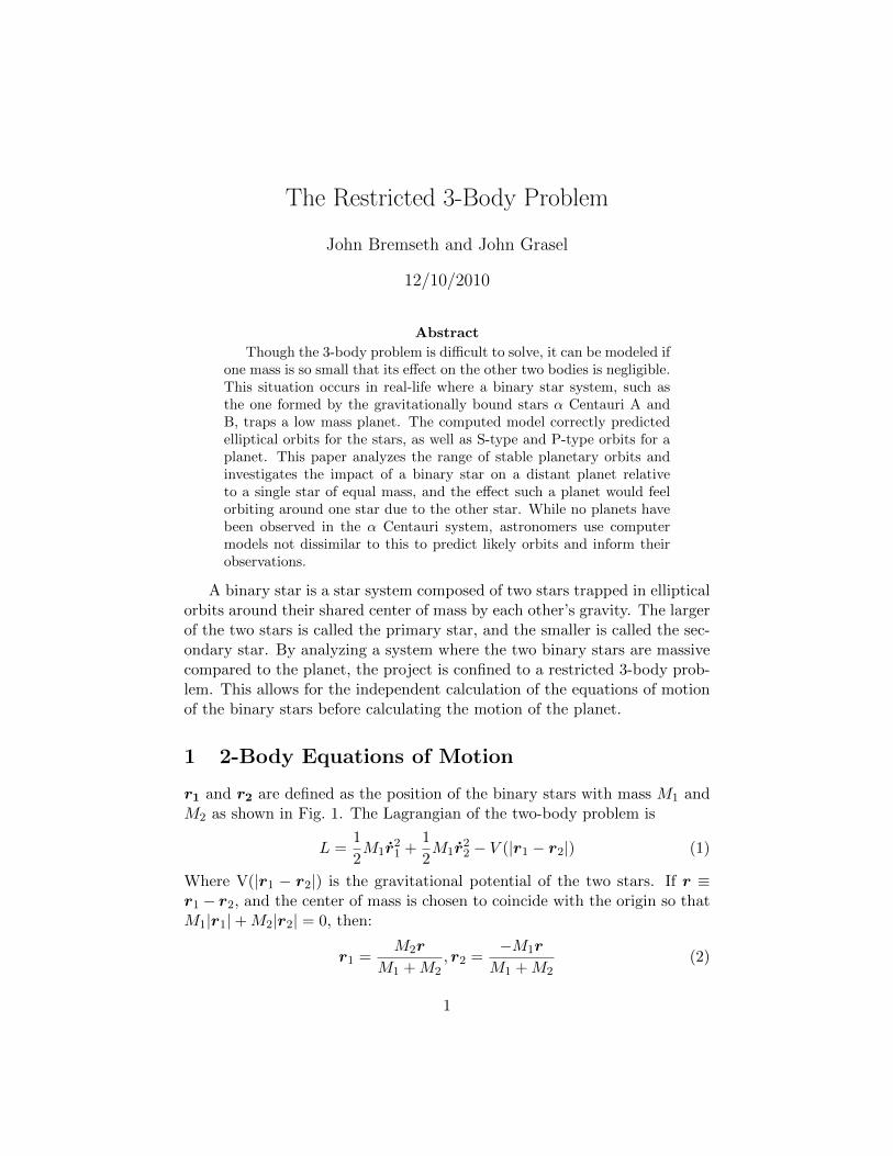
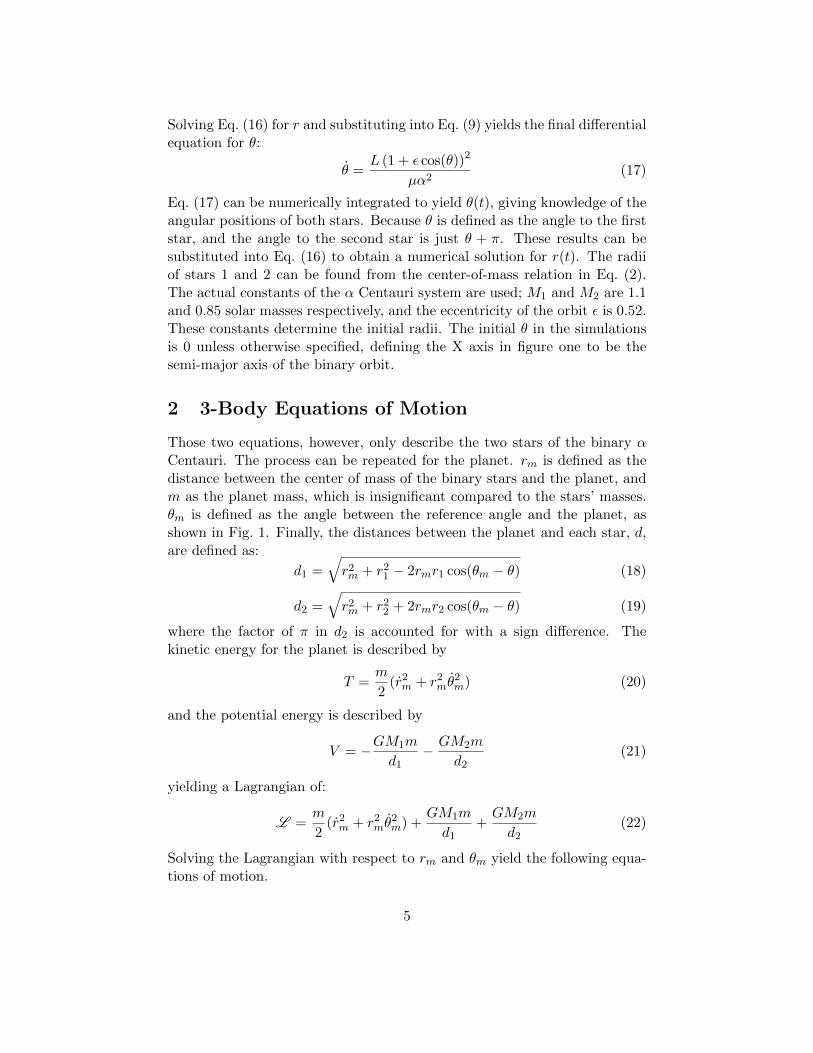
The binary star system has thus been reduced to a single body of mass µorbiting a fixed point, the center of mass of the binary system, at radius rand angle θ as shown in Fig. 2. If r is defined as |r| and θ is defined asthe angle between M1 and the semi-major axis as shown in Fig. 1, then the

rm

r

r1

r2

θm

θ

m

M1

M2

d1d2

y

x

Friday, December 10, 2010

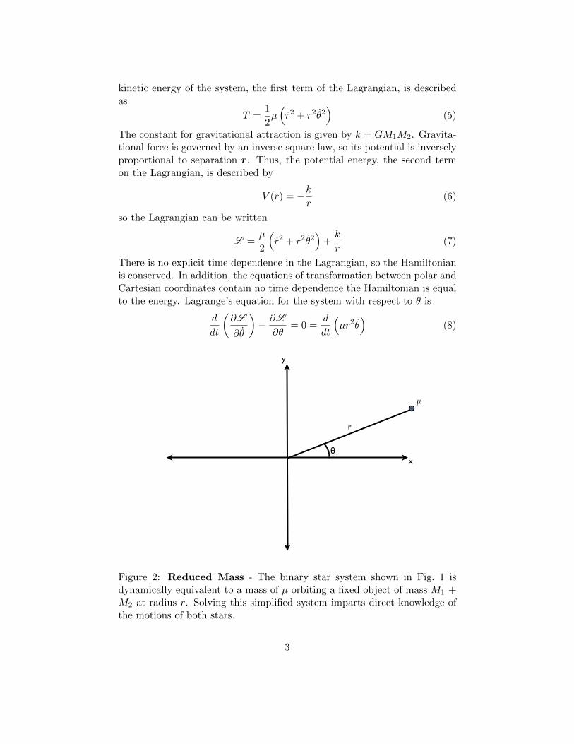
Figure 1: Setup - System diagram for modeling the motion of the binarystars (M1 and M2) and the planet (m). To simplify the diagrammed 3-bodyproblem, m is approximated to be very small compared to M1 and M2. Thus,the motion of the stars can be calculated first (the 2-body problem) and themotion of the planet can be added in later (the restricted 3-body problem).The origin represents the center of mass of the binary star system.

2

kinetic energy of the system, the first term of the Lagrangian, is describedas

T =1

2µ(r2 + r2θ2

)(5)

The constant for gravitational attraction is given by k = GM1M2. Gravita-tional force is governed by an inverse square law, so its potential is inverselyproportional to separation r. Thus, the potential energy, the second termon the Lagrangian, is described by

V (r) = −kr

(6)

so the Lagrangian can be written

L =µ

2

(r2 + r2θ2

)+k

r(7)

There is no explicit time dependence in the Lagrangian, so the Hamiltonianis conserved. In addition, the equations of transformation between polar andCartesian coordinates contain no time dependence the Hamiltonian is equalto the energy. Lagrange’s equation for the system with respect to θ is

d

dt

(∂L

∂θ

)− ∂L

∂θ= 0 =

d

dt

(µr2θ

)(8)

r

θ

�

y

x

Friday, December 10, 2010

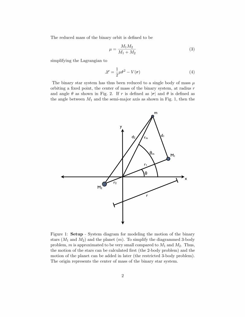
Figure 2: Reduced Mass - The binary star system shown in Fig. 1 isdynamically equivalent to a mass of µ orbiting a fixed object of mass M1 +M2 at radius r. Solving this simplified system imparts direct knowledge ofthe motions of both stars.

3

Eq. (8) is a statement of conservation of angular momentum, L, defined as

L ≡ µr2θ (9)

From here, Lagrange’s equations could be calculated with respect to r, andthe product, two differential equations, could be numerically solved. How-ever, due to conservation of linear and angular momentum, solving for θ as afunction of time defines the binary system. Thus two differential equationswould be redundant, and reducing the system to only one speeds compu-tational time and simplifies the system. For this, radial dependence withinthe differential equation for θ must be removed. To accomplish this, thesystem’s energy

E = T+V =µ

2

(r2 + r2θ2

)−kr

=µ

2

(r2 + r2

L2

µ2r4

)−kr

=µ

2

(r2 +

L2

µ2r2

)−kr

(10)is used. Solving Eq. (10) for r2 yields,

r2 =2

µ

(E −

(L2

2µr2− k

r

))(11)

and substituting in Eq. (9) and Eq. (11), the relation

dr

dθ=r

θ=

√2µ

(E −

(L2

2µr2− k

r

))L/µr2

(12)

is formed. Changing variables from r = 1/u; making the appropriate substi-tutions and defining u and u as derivatives of u with respect to θ, the aboveequation of motion becomes

du

dθ= −µ

L

√2

µ

(E −

(L2u2

2µ− ku

))(13)

Squaring both sides and differentiating with respect to θ,

2uu = −2µ

L2

(dE

dθ− L2u2

2µ(2uu) + ku

)(14)

where the system’s rotational symmetry guarantees that dEdθ is zero. The

equation for the inverse radius with no explicit θ dependence is thus

u+ u =kµ

L2(15)

Defining α = L2/µk and ε =√

1 + 2EL2/µk2, the solution to Eq. (15) is

α

r= 1 + ε cos(θ) (16)

4

Solving Eq. (16) for r and substituting into Eq. (9) yields the final differentialequation for θ:

θ =L (1 + ε cos(θ))2

µα2(17)

Eq. (17) can be numerically integrated to yield θ(t), giving knowledge of theangular positions of both stars. Because θ is defined as the angle to the firststar, and the angle to the second star is just θ + π. These results can besubstituted into Eq. (16) to obtain a numerical solution for r(t). The radiiof stars 1 and 2 can be found from the center-of-mass relation in Eq. (2).The actual constants of the α Centauri system are used; M1 and M2 are 1.1and 0.85 solar masses respectively, and the eccentricity of the orbit ε is 0.52.These constants determine the initial radii. The initial θ in the simulationsis 0 unless otherwise specified, defining the X axis in figure one to be thesemi-major axis of the binary orbit.

2 3-Body Equations of Motion

Those two equations, however, only describe the two stars of the binary αCentauri. The process can be repeated for the planet. rm is defined as thedistance between the center of mass of the binary stars and the planet, andm as the planet mass, which is insignificant compared to the stars’ masses.θm is defined as the angle between the reference angle and the planet, asshown in Fig. 1. Finally, the distances between the planet and each star, d,are defined as:

d1 =√r2m + r21 − 2rmr1 cos(θm − θ) (18)

d2 =√r2m + r22 + 2rmr2 cos(θm − θ) (19)

where the factor of π in d2 is accounted for with a sign difference. Thekinetic energy for the planet is described by

T =m

2(r2m + r2mθ

2m) (20)

and the potential energy is described by

V = −GM1m

d1− GM2m

d2(21)

yielding a Lagrangian of:

L =m

2(r2m + r2mθ

2m) +

GM1m

d1+GM2m

d2(22)

Solving the Lagrangian with respect to rm and θm yield the following equa-tions of motion.

5

rm = rmθ2m −GM1

rm − r1 cos(θm − θ)d3/21

−GM2rm + r2 cos(θm − θ)

d3/22

(23)

2rmrmθ + r2mθm = −GM1rmr1 sin(θm − θ)

d3/21

+GM2rmr2 sin(θm − θ)

d3/22

(24)

These equations are numerically solvable using Mathematica. The planet’sinitial position and velocity (r, r, θ, and θ) are defined relative to the centerof mass of the binary system. These are specified on the plots only if nonzero.

3 Results

As predicted, the simulation of the binary system shows the binary starscompleting their orbits with a period of 80 years as seen in Fig. 3. Themassive star orbits more closely to the center of mass than the lighter star,and the stars are observed moving more rapidly near the barycenter, thebinary stars’ center of mass, of the system. The graphics depict the passageof time through the coloring of the orbit: purple represents the beginning ofthe simulation, and the color gradient represents passage of time. Because

-20 -15 -10 -5 5 10 15X HAUL

-10

-5

5

10

Y HAUL

Figure 3: Binary Star System - The two stars in the α Centauri systemorbit each other elliptically with a period of 80 years. The coloring of thesystem depicts the passage of time which evolves from purple to red. Forthis and following simulations, the stars begin their orbits at Perigee.

6

-60 -40 -20 20 40 60X HAUL

-80

-60

-40

-20

20

40

60

Y HAULICs: Θ':0.01517, Planet R 70.

Figure 4: P-Type Orbit - The planet orbits both binary stars. Theconstantly-changing positions of the two inner stars cause small changesin the radius of the planet’s orbit, but the orbit remains stable for over 7000years. The actual orbit radii are very close to the predictions of a planet’sradius about a single star with the mass of both binary stars if given thesame initial conditions.

color maps linearly to time, a region of rapid color change is brought by lowvelocity, and slow color change by high velocity. All subsequent simulationsfollow this color convention.

The model predicts two different types of orbits for the planet’s motion:the P-type orbit characterized by the planet orbiting both stars, and theS-type characterized by the planet orbiting only one of the stars. P-typeorbits were found to be stable at large distances from the binary stars. At

7

these distances, the two stars behavior can be approximated as a single starat the system’s barycenter. Experimentation with various initial conditionsthat resulted in circular orbits yielded a closest stable orbit radius of ≈ 70AU, very close to the single-star approximation radius of 69.4 AU. This orbitis shown in Fig. 4.

To generate an P-Type orbit, initial conditions requisite for a circularorbit with constant radius r of a planet of mass m around the total mass ofthe binary stars:

mv2

r=mr2θ2

r= mrθ2 =

GMm

r2

θ =

√GM

r3(25)

where M = M1 + M2. Solving this equation for r yields the single-starapproximation radius. At a close distance to the stars, like 70 AU, theplanet’s orbit is noticeably different from circular. Closer orbits becomeincreasingly sensitive to the binary nature of the star system, and theirorbits disintegrate more rapidly.

S-type planetary orbits occurred in the regions around each member ofthe binary. Stable orbits were found up to 5 AU away from the less massivestar, as shown in Fig. 5, and up to 3 AU away from the more massive star.

The same basic process for generating stable P-type orbits can be usedto generate stable S-type orbits. Rather than calculate the radius of theplanet’s travel around the barycenter, Eq. (25) is solved for the circularorbit radius about one of the stars. The M in Eq. (25) then represents themass of the primary or secondary star. In addition, a second term must beadded to this calculated angular velocity to account for the motion of thestar. Thus, the only motion apparent in the star’s center of mass frame isthe desired circular orbit.

Of course, not all orbits conceived in this manner are stable due to theinfluence of the second star. Stability is tested for by giving the planet asmall initial r in either direction and ensuring that the orbit approaches oroscillates about the same steady state radius. Orbits far away from theircentral star are increasingly affected by the other star. As expected, thesmaller the radius of orbit, the less deviation from the ideal single-star cir-cular orbit is observed. An example of a tight orbit is shown Fig. 6 to becontrasted with the large disturbances seen in Fig. 5.

The tight orbit is better understood when viewed in the frame of itsparent star, as shown in Fig. 9. While the orbit is clearly elliptical, it is notwildly so, and its ellipticity can be seen to vary throughout the period of thebinary, decreasing when the binary approaches apogee and increasing whenthe binary reaches perigee. In order to more clearly observe the dependenceof the planet’s motion on the star’s motion, both the X and Y components

8

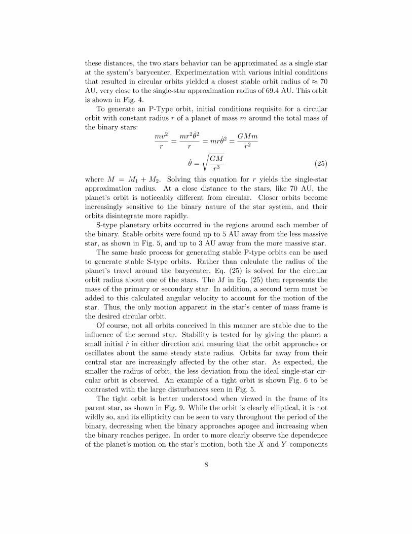
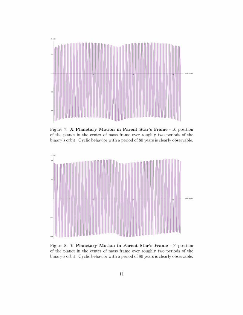
of the planet’s motion in the parent star’s frame are plotted over severalperiods of the binary’s orbit in figures Fig. 7 and Fig. 8 respectively.

The graphical results suggest that the radius’ deviations are periodic witha period similar to the period of the binary system. A Fourier transformprovides a way to further test this hypothesis. Taking the Fourier transformof the X component of the planet’s orbital radius over a timescale thatencompassed multiple 80-year periods yields the frequency domain analysisshown in Fig. 10.

In Fig. 10, the first independent peak corresponds to the orbital periodof the planet around its parent star at 1.051 inverse years. This figure agreeswith its observed rotation. More interesting however are the several smallerpeaks that surround the primary one. These peaks can be more clearlyobserved in Fig. 11, which displays the Fourier analysis only in neighborhoodof the peak of interest. The peaks on either side of the primary are exactly

-20 -15 -10 -5 5 10 15X HAUL

-10

-5

5

10

Y HAULICs: Planet R 10.1, Planet R' 0.1

Figure 5: S-Type Orbit - A planet orbits one of the two binary stars.Notice how much the secondary star affects the planet’s motion. The effectis most evident at the semi-major axis. Because the stars elliptical orbitsreturn to the same position after 80 years, in a long simulation like thisone, the stars overwrite their old positions. In this figure, neither star has apurple region because the orange region is on top of it.

9

-20 -10 10 20X HAUL

-10

-5

5

10

Y HAULICs: Planet R 5. Planet d�dt 1.35

Figure 6: A Tighter Orbit - The closer the planet is to one of the twostars, the less affected it is by the other.

0.0125 inverse years away, and the spacing between all subsequent peaksis roughly the same value. 0.0125 inverse years is significant because itcorresponds to an 80 year period, exactly that of the binary. Clearly this isevidence for some form of dependence on the binary orbit, though the natureof this dependence has not been determined. It should be noted that thesecontributions are very small compared to that of the planet’s orbit, and canbe left for future work.

While it was originally believed that these peaks were some residue ofthe Fourier analysis, the fact that the space between them exactly corre-sponded to the period of the binary suggests that they are not. In addition,experiments in varying both the sampling rate and sample size yielded nochange in the structure or placement the peaks, leading to the conclusionthat this phenomena must be physical.

In addition to S- and P-type orbits, interesting behavior was observedin unstable orbits when the planet was pulled too close to one star. This“collision” resulted in the planet’s ejection from the system. Since our modelapproximates the planets and stars as points and does not conserve energydue to the massive approximation, a better model is necessary to gain intu-ition on planet ejection.

Unfortunately, the investigation into the existence of figure-eight plane-tary orbits around both stars was unsuccessful. Any such orbits, if they doexist, must be highly unstable and repulsive. While such analysis would be

10

50 100 150Time HYearsL

-1.0

-0.5

0.5

X HAUL

Figure 7: X Planetary Motion in Parent Star’s Frame - X positionof the planet in the center of mass frame over roughly two periods of thebinary’s orbit. Cyclic behavior with a period of 80 years is clearly observable.

50 100 150Time HYearsL

-1.0

-0.5

0.5

1.0

Y HAUL

Figure 8: Y Planetary Motion in Parent Star’s Frame - Y positionof the planet in the center of mass frame over roughly two periods of thebinary’s orbit. Cyclic behavior with a period of 80 years is clearly observable.

11

-1.0 -0.5 0.5X HAUL

-1.0

-0.5

0.5

1.0

Y HAUL

Figure 9: Tight Orbit in Parent Star’s Frame - Orbiting around itsparent star at the origin, the planet executes a nearly circular path. Theellipticity of its orbit becomes less as the binary orbit approaches apogee.

outside of the scope of this project, it would be interesting to calculate theRoche lobe analytically. Since the Roche lobe is a constant-energy surfaceshaped like a figure-eight, initial conditions that caused a planet to stay nearthis surface might yield such an orbit.

During the search, some interesting planetary orbits were discovered.One such orbit is P-type, but maintains a separation of roughly 5 AU fromits parent star. As such, it is heavily influenced by the secondary star, asshown in Fig. 12; in fact, at its closest approach, the planet is nearly asclose to the less massive secondary star as it is to the primary star. Whilethis arrangement usually resulted in instability, this particular set of initialconditions results in a stable orbit for over 500 years. This may be dueto a near-integral number of planet-star rotations (≈7) for every star-star

12

2 4 6 8 10Frequency H1�YearsL

10-16

10-11

10-6

0.1

104

Power

Figure 10: Fourier Transform - Fourier Transform sampling 10000 yearsof data at intervals of .05 years. A strong peak is observed at 1.051 inverseyears corresponding to the orbit of the planet around its parent star.

0.7 0.8 0.9 1.0 1.1 1.2 1.3Frequency H1�YearsL10-18

10-14

10-10

10-6

0.01

100

Power

Figure 11: Fourier Transform - Fourier Transform sampling 10000 years ofdata at intervals of .05 years. The window is restricted to the region containthe strong peak observed in Fig. 10. Surrounding this peak are several evenlyspaced peaks several orders of magnitude weaker than the central one. Thespacing between the peaks was determined to be exactly .0125 inverse years,corresponding to a period of 80 years.

13

rotation.A second area of interest was to ascertain the possibility of a planet

switching from a P-type orbit around one star to a P-type orbit around theother. A more interesting orbit was found: the system in Fig. 13 startedorbiting around the less massive star, switched to an orbit around the otherstar, and switched back to the first star. This system was not stable, becauseeventually the planet was ejected from the system or collided with one ofthe stars.

4 Conclusion

The restricted 3-body problem was successfully solved. The model predictsthe existence of stable planetary orbits around binary stars, both of typeS and P. Fourier analysis identified that the binary nature of the systemresulted in small but measurable disturbances in both S and P type orbits.

14

-20 -10 10 20X HAUL

-15

-10

-5

5

10

15Y HAUL

ICs: Orientation45°, Planet R -5.0415276, R' 2.98766715

Figure 12: Orbital Shifting - A planet orbits one of the binary stars, butis influenced by the other. The frequency of its orbit around its star is closeto, but not exactly, an integer multiple of the frequency of the binary starsystem, resulting in a gradual rotation of the planet’s orbit over time.

-20 -10 10X HAUL

-15

-10

-5

5

10

15

Y HAULICs: Planet R 11., Planet R' 9.026194844178638*^-21

Figure 13: Orbital Switching - The planet starts orbiting one star, butswitches to the other star and back again. Such a system is highly unstableand is not observed in nature.

15