Embed Size (px)
Citation preview
Electronic copy available at: https://ssrn.com/abstract=2983514
Crawford School of Public Policy
CAMACentre for Applied Macroeconomic Analysis
The role of border carbon adjustments in a US carbon tax
CAMA Working Paper 39/2017June 2017
Warwick J. McKibbinCrawford School of Public Policy, ANUThe Brookings Institution and Centre for Applied Macroeconomic Analysis, ANU
Adele C. MorrisThe Brookings Institution and Centre for Applied Macroeconomic Analysis, ANU
Peter J. WilcoxenSyracuse UniversityThe Brookings Institution and Centre for Applied Macroeconomic Analysis, ANU
Weifeng LiuCentre for Applied Macroeconomic Analysis, ANU
Abstract
This paper examines carbon tax design options in the United States using an intertemporal computable general equilibrium model of the world economy called G-Cubed. Four policy scenarios explore two overarching issues: (1) the effects of a carbon tax under alternative assumptions about the use of the resulting revenue, and (2) the effects of a system of import charges on carbon-intensive goods (“border carbon adjustments”).
| T H E A U S T R A L I A N N A T I O N A L U N I V E R S I T Y
Electronic copy available at: https://ssrn.com/abstract=2983514
Keywords
JEL Classification
Address for correspondence:
ISSN 2206-0332
The Centre for Applied Macroeconomic Analysis in the Crawford School of Public Policy has been established to build strong links between professional macroeconomists. It provides a forum for quality macroeconomic research and discussion of policy issues between academia, government and the private sector.The Crawford School of Public Policy is the Australian National University’s public policy school, serving and influencing Australia, Asia and the Pacific through advanced policy research, graduate and executive education, and policy impact.
| T H E A U S T R A L I A N N A T I O N A L U N I V E R S I T Y

Electronic copy available at: https://ssrn.com/abstract=2983514
THE ROLE OF BORDER CARBON ADJUSTMENTS IN A U.S. CARBON TAX
MAY 31, 2017
WARWICK J. MCKIBBIN Australian National University
Brookings
ADELE C. MORRIS Brookings
PETER J. WILCOXEN
Syracuse University Brookings
WEIFENG LIU
Australian National University
The Brookings Institution is a private non-profit organization. Its mission is to conduct high quality, independent research and, based on that research, to provide innovative, practical recommendations for policymakers and the public. The conclusions and recommendations of any Brookings publication are solely those of its author(s), and do not reflect the views of the Institution, its management, or its other scholars. Support for this publication was generously provided by the Alex C. Walker Foundation. Authors thank Nicholas Montalbano for his research assistance. Brookings recognizes that the value it provides is in its absolute commitment to quality, independence and impact. Activities supported by its donors reflect this commitment and the analysis and recommendations are not determined or influenced by any donation.
EXECUTIVE SUMMARY
This paper examines carbon tax design options in the United States using an intertemporal computable general equilibrium model of the world economy called G-Cubed. Four policy scenarios explore two overarching issues: (1) the effects of a carbon tax under alternative assumptions about the use of the resulting revenue, and (2) the effects of a system of import charges on carbon-intensive goods (“border carbon adjustments”). We first establish a baseline scenario in which the United States does not adopt a climate policy other than policies in place in early 2017. Then we model a simple excise tax on the carbon content of fossil fuels in the U.S. energy sector starting in 2020 at $27 per metric ton of carbon dioxide (CO2) and rising at 5 percent above inflation each year through 2050. We investigate two approaches to using the revenue: one that rebates the revenue to households in annual lump sum transfers (LS below) and one that applies the revenue to reduce the marginal tax rate on capital income (KT below). For each revenue policy, we run scenarios with and without a border carbon adjustment (BCA) on imports. The BCAs vary by country and good and account for the carbon emitted throughout the full production chain of the good in the country where it is produced. Consistent with earlier studies, we find that the carbon tax raises considerable revenue and reduces CO2 emissions significantly relative to baseline, no matter how the revenue is used. Gross annual revenue from the carbon tax with lump sum rebating and no BCA begins at $110 billion in 2020 and rises gradually to $170 billion in 2040. By 2040, annual CO2 emissions fall from 5.5 billion metric tons (BMT) under the baseline to 2.4 BMT, a decline of 3.1 BMT, or 57 percent. Cumulative emissions over 2020 to 2040 fall by 48 BMT. Also consistent with earlier studies, we find that the carbon tax has very small overall impacts on GDP, wages, employment, and consumption. Different uses of the revenue from the carbon tax result in slightly different levels and compositions of GDP across consumption, investment and net exports. Overall, using carbon tax revenue to reduce the capital income tax rate results in better macroeconomic outcomes than using the revenue for lump sum transfers. Indeed, even while achieving remarkable emissions reductions, the policy results in the U.S. economy reaching the output projections in 2040 only about three months later than it would without the carbon tax. With the rebates, consumption rises in the short run and then returns close to baseline in the medium to longer run. Investment falls sharply in the short to medium run and recovers somewhat in the long run, but remains about one percentage point below baseline. In contrast, the capital tax reduction has little effect on consumption in the short run and causes investment to rise briefly relative to baseline before it settles within a half percentage point from baseline in the long run.
2

Counter to their purported purpose of protecting U.S. trade strength, for a given revenue policy, BCAs tend to produce lower net exports than the carbon taxes alone. This is generally because the BCAs result in higher value of the dollar relative to other currencies, thus lowering exports more than they lower imports. This is consistent with standard results in the international trade literature on the effects of import tariffs and export subsidies on real exchange rates, a result that is often ignored in the discussion of domestic carbon policy. In a finding new to the literature, our results show that BCAs can have strikingly different effects depending on the use of the revenue. The BCAs in the lump sum rebate scenario result in slightly lower domestic output than the same scenario without the BCAs, thus doing more harm than good -- including in the relatively energy-intensive sectors like durable goods manufacturing. In contrast, BCAs tend to result in higher output than the carbon tax alone when the revenue is used to reduce other distortions in the economy.
3

1. INTRODUCTION
Two important design choices for a U.S. carbon tax policy are the use of the revenue and whether and how to include measures to address the competitiveness concerns of American businesses. Both of these policy design choices affect the political appeal and overall performance of the policy, and their effects can be interdependent. For example, a carbon tax that funds reductions in corporate income tax rates could make U.S. firms more competitive overall than they otherwise might have been. Using a model of the global economy, this paper explores the effect of an illustrative carbon tax on U.S. macroeconomic outcomes with special attention to these trade-related policy design options. Because climate policies and effective carbon prices vary widely across countries, a unilateral carbon tax instituted in the United States could in principle promote the relocation of economic activity from the United States to regions with less ambitious climate policy, resulting in an offset to the environmental gains achieved by the United States. This is known as emissions leakage.1 Unilateral carbon pricing would be particularly likely to lower output and employment in American energy-intensive trade-exposed (EITE) sectors by hurting their global competitiveness. On the other hand, if the United States adopts a carbon tax that slows its economic growth, that in turn may lower growth in other countries and thereby reduce their carbon emissions relative to baseline. We call this phenomenon “negative leakage.” So the question arises whether, where, and in which sectors emissions leakage is positive or negative, and what the overall effect would be on global emissions. To decompose the various forces that drive leakage, this study simulates a unilateral U.S. carbon tax with a computable general equilibrium model of the global economy called G-Cubed. The second question we address here is the effect of measures that could counteract the potential for positive leakage and ameliorate the concerns of domestic EITE industries. 2 A number of options appear in the literature, each of which comes with important tradeoffs,3
1 Here we refer to the leakage that occurs through shifts in emissions-intensive industry locations. Price-based leakage occurs when fossil fuel consumption in countries without carbon constraints increases as a result of a decrease in demand and prices of traded fossil fuels. This leakage channel cannot be addressed by a border carbon adjustment or similar policy. 2 Fischer and Fox, 2012a; Condon and Ignaciuk, 2013. 3 For a succinct summary of these pros and cons, see Fischer et al. (2015)
4

design challenges,4 and questions of consistency with current World Trade Organization (WTO) law.5 For example, policymakers could partially or fully exempt EITE sectors from the carbon tax or give rebates to EITE firms based on their output levels. Arguably the most prominent option is a border carbon adjustment (BCA). The carbon tax itself would apply to the carbon content of imported fossil fuels, whereas a BCA would apply to goods other than fossil fuels. In practice, a BCA would apply to goods imported from countries that do not price carbon at a level at least as high as the carbon price in the United States.6 In principle, this would help ensure that the U.S. carbon tax does not disadvantage emission-intensive goods produced in the United States relative to emission-intensive goods produced in foreign countries without a similar climate policy. A BCA on imports (which we model here) could vary by country and good, based on the average carbon intensity of production. For example, if the carbon tax in the United States is $30 per metric ton of CO2, and steel produced in Country X involves emissions of five metric tons of CO2 per unit in its supply chain, the BCA would impose a charge of $150 for every unit of steel the United States imports from Country X. The idea is that this charge would prevent unfair competition to steelmakers in the United States as a result of lower environmental standards abroad, and in principle such a charge could incentivize the exporting country to reduce its emissions. To be sure, a host of details arise, such as exactly how to calculate CO2 emissions for steel in Country X (for example by firm, region, production process, or using an industry average), how to differentiate across different kinds of steel, and whether and how to account for differences between County X’s policies and those of the United States. An export BCA would rebate the carbon tax liability producers incur in making goods they export from the United States. This would help U.S. exports of emission-intensive goods remain competitive in countries without similarly-stringent climate policies. Analysts generally agree that a BCA on imports would likely satisfy the requirements for an environmental exception under WTO law as long as the adjustment is no greater than the domestic carbon tax. An export BCA may more difficult to justify in the case of a WTO dispute because its justification is trade competitiveness, not environmental protection.7 We restrict our focus here to a border carbon adjustment on imports, and in our conclusions we speculate as to how our results might differ with a BCA on exports as well.
4 See, for example, Kortum and Wesibach (2016); CBO (2013); Sakai and Barrett (2016); Cosbey (2008); Branger and Quirion (2014); Böhringer et al. (2012) 5 For a full discussion of WTO law constraints on BCAs and similar policies, see Trachtman (2016) 6 A question arises about how a BCA should apply to goods from countries that apply a carbon price at a level below that of the United States, but at a rate above zero. We abstract from that in our modeling by assuming countries either have analogous policies or no climate policy. 7 Trachtman (2016)
5
A number of studies have explored leakage and competitiveness and policy options to address them. For example, Böhringer et al. (2012) find that overall leakage rates in the range of 5 to 20 percent. McKibbin et al. (2012a), in contrast, find no evidence of energy-related emissions leakage. The estimated magnitudes of the effects vary by industry as well, with EITE industries disproportionately affected (Fischer and Fox, 2012b). Aldy and Pizer (2009) estimate that vulnerable EITE industries with energy costs that exceed ten percent of shipment value would expect at most a one percent shift in production overseas. A large literature demonstrates how carbon taxes can both lower emissions and raise a substantial amount of revenue (CBO, 2011; McKibbin et al., 2012b; Rausch and Reilly, 2015). Previous literature finds that the macroeconomic impact of a carbon tax depends significantly on the use of revenue. If the revenue is used to fund reductions in other distortionary taxes, the tax reductions can offset the macroeconomic drag of the carbon tax (i.e., a weak double dividend).8 Generally, research shows that using the revenue to reduce the marginal rates of distortionary taxes such as those on capital and labor income produces better aggregate welfare than using it for lump sum rebates, although the lump sum rebates can produce more progressive distributional outcomes.9 In this paper, we examine a simple excise tax on the carbon content of fossil fuels in the U.S. energy sector starting in 2020 at $27 per metric ton of carbon dioxide (CO2) and rising at 5 percent above inflation each year through 2050 and remaining constant thereafter. The tax revenue either returns to households in rebates or funds reductions in the marginal tax rate on capital income, and we model both approaches with and without a BCA on imports. We do this using the G-Cubed model, a global intertemporal computable general equilibrium (CGE) model, which allows us to explore the possible effects of emissions control policies on: the U.S. macroeconomy; individual industrial sectors within the United States; and other outcomes, such as trade flows, currency values, emissions levels, and economic activity. Our baseline and policy scenarios do not account for the economic damages that would result from a disrupted climate. These unaccounted-for damages and the benefits of emissions mitigation are likely to be particularly important in the later years of our modeling time horizon. Since our analytical approach does not quantify the economic effects of climate change, this study does not elucidate the potential net benefits of a carbon tax. Indeed, the benefits of
8 Goulder, 1995; Jorgenson et al., 2013 9 McKibbin et al 2015; Tuladhar et al., 2015; Jorgenson et al., 2015; Elmendorf, 2009.
6

avoided damages may be well in excess of the costs we report for emissions control. Rather, our focus here is on the relative economic outcomes of the different policy designs with equivalent environmental outcomes, consistent with the very similar cumulative emissions in our policy scenarios. The paper is structured as follows. Section 2 describes the model, the baseline (no policy) scenario, and four policy scenarios. Section 3 reviews the results. Section 4 concludes. 2. MODELING APPROACH AND SCENARIOS
In this section we present a brief overview of the G-Cubed model and its features that are most relevant for our analysis. An extended technical discussion of G-Cubed appears in McKibbin and Wilcoxen (2013) and a more detailed description of the theory behind the model can be found in McKibbin and Wilcoxen (1999).10 The version of G-Cubed we use in this study includes the nine geographical regions listed in Table 1 below. The United States, Japan, Australia, and China are each represented by a separately modeled region. The model aggregates the rest of the world into five composite regions: Western Europe, the rest of the OECD (not including Mexico and Korea); Eastern Europe and the former Soviet Union; OPEC oil exporting economies; and all other developing countries.
Table 1: Regions in the G-Cubed Model
Region Code Region Description US United States
Japan Japan Aus Australia Eur Western Europe
ROECD Rest of the OECD, i.e. Canada and New Zealand China China EEFSU Eastern Europe and the former Soviet Union LDC Other Developing Countries
OPEC Oil Exporting Developing Countries
10 The type of CGE model represented by G-Cubed, with macroeconomic dynamics and various nominal rigidities, is closely related to the dynamic stochastic general equilibrium models that appear in the macroeconomic and central banking literatures.
7

The full list of sectors in the model is shown in Table 2. The “code” column provides short names for the sectors that will appear in tables and graphs of results. G-Cubed’s electricity sector includes specific technologies: coal, natural gas, oil, nuclear, wind, solar, hydro and other (largely biomass and other renewables). A technical discussion of modeling improvements to the electricity sector appears in McKibbin et al. (2015).
Table 2: Sectors in the G-Cubed Model
Num Sector Name Code Notes 1 Electricity delivery ElecU
Primary Energy
2 Gas utilities GasU 3 Petroleum refining Ref 4 Coal mining CoalEx 5 Crude oil extraction CrOil 6 Natural gas extraction GasEx 7 Other mining Mine
Nonenergy Traded Goods
8 Agriculture and forestry Ag 9 Durable goods Dur 10 Nondurables NonD 11 Transportation Trans 12 Services Serv 13 Coal generation Coa
Electricity Generation
14 Natural gas generation Gas 15 Petroleum generation Oil 16 Nuclear generation Nuc 17 Wind generation Win 18 Solar generation Sun 19 Hydroelectric generation Hyd 20 Other generation Oth
The Baseline Scenario The model’s projections of future emissions and economic activity in the absence of new climate policy is our business-as-usual (baseline) scenario. A detailed discussion of the baseline construction process for G-Cubed appears in McKibbin, Pearce and Stegman (2009). The baseline in this study is broadly consistent with the emissions and GDP growth in the Energy Information Administration’s Annual Energy Outlook Early Release, No Clean Power Plan case
8
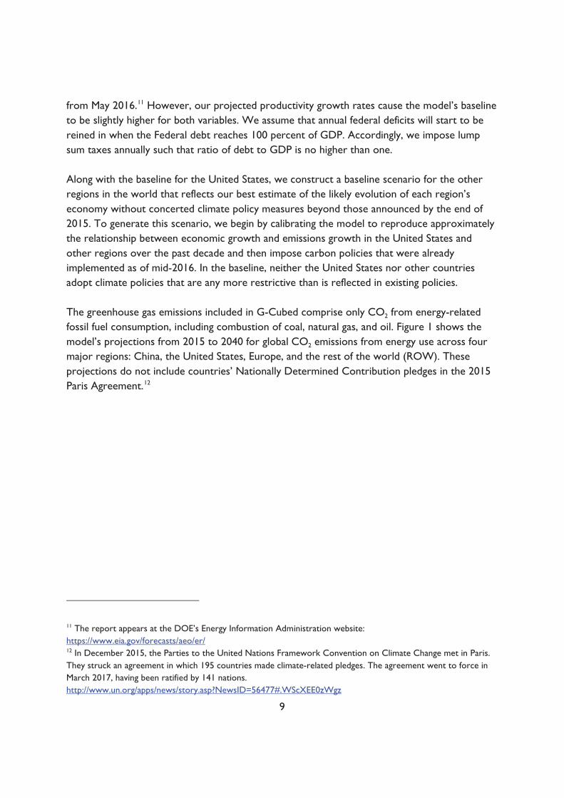
from May 2016.11 However, our projected productivity growth rates cause the model’s baseline to be slightly higher for both variables. We assume that annual federal deficits will start to be reined in when the Federal debt reaches 100 percent of GDP. Accordingly, we impose lump sum taxes annually such that ratio of debt to GDP is no higher than one. Along with the baseline for the United States, we construct a baseline scenario for the other regions in the world that reflects our best estimate of the likely evolution of each region’s economy without concerted climate policy measures beyond those announced by the end of 2015. To generate this scenario, we begin by calibrating the model to reproduce approximately the relationship between economic growth and emissions growth in the United States and other regions over the past decade and then impose carbon policies that were already implemented as of mid-2016. In the baseline, neither the United States nor other countries adopt climate policies that are any more restrictive than is reflected in existing policies. The greenhouse gas emissions included in G-Cubed comprise only CO2 from energy-related fossil fuel consumption, including combustion of coal, natural gas, and oil. Figure 1 shows the model’s projections from 2015 to 2040 for global CO2 emissions from energy use across four major regions: China, the United States, Europe, and the rest of the world (ROW). These projections do not include countries’ Nationally Determined Contribution pledges in the 2015 Paris Agreement.12
11 The report appears at the DOE’s Energy Information Administration website: https://www.eia.gov/forecasts/aeo/er/ 12 In December 2015, the Parties to the United Nations Framework Convention on Climate Change met in Paris. They struck an agreement in which 195 countries made climate-related pledges. The agreement went to force in March 2017, having been ratified by 141 nations. http://www.un.org/apps/news/story.asp?NewsID=56477#.WScXEE0zWgz
9

Figure 1: Global Baseline Carbon Dioxide Emissions
The Policy Scenarios In this study, we examine an illustrative carbon tax imposed in the United States but not in other countries. The tax applies economy-wide to all sources of CO2 emissions from fossil energy use. To the extent that trade and investment may be distorted by climate policy, those outcomes are most likely to be apparent in such a unilateral context. Thus, in our scenarios without border measures, we are likely estimating the upper bound on competitiveness effects. As shown in Figure 2,13 we impose the tax beginning in 2020, starting at $27 per metric ton of CO2, and we increase the tax rate annually by 5 percent over inflation. By 2040, the final year we report for our simulations in this paper, the tax is $72 per metric ton. In years after 2050, which are relevant for agents in the model with forward-looking expectations, we hold the carbon tax rate constant at its 2050 level of $117. We assume the carbon tax is anticipated, not a surprise.
13 Unless otherwise indicated, all dollar values are in 2015 dollars.
010
2030
4050
Billi
on M
etric
Ton
s
2015 2020 2025 2030 2035 2040
China ROW US Europe
10
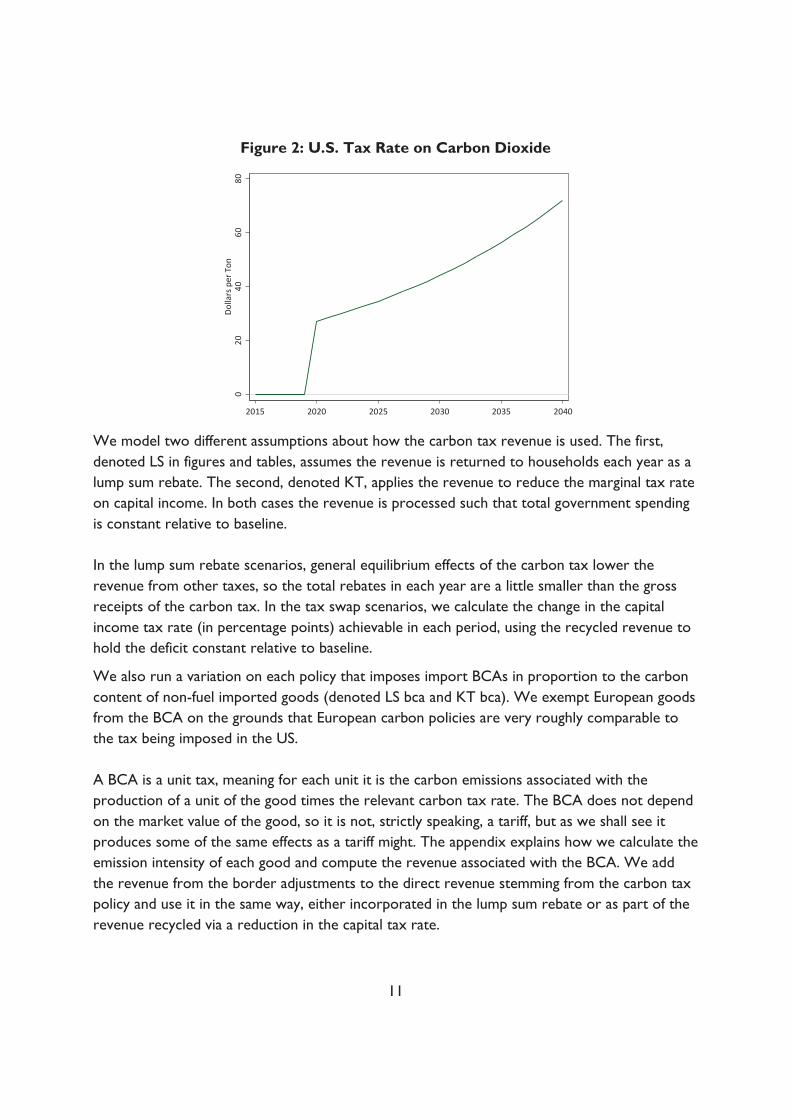
Figure 2: U.S. Tax Rate on Carbon Dioxide
We model two different assumptions about how the carbon tax revenue is used. The first, denoted LS in figures and tables, assumes the revenue is returned to households each year as a lump sum rebate. The second, denoted KT, applies the revenue to reduce the marginal tax rate on capital income. In both cases the revenue is processed such that total government spending is constant relative to baseline. In the lump sum rebate scenarios, general equilibrium effects of the carbon tax lower the revenue from other taxes, so the total rebates in each year are a little smaller than the gross receipts of the carbon tax. In the tax swap scenarios, we calculate the change in the capital income tax rate (in percentage points) achievable in each period, using the recycled revenue to hold the deficit constant relative to baseline.
We also run a variation on each policy that imposes import BCAs in proportion to the carbon content of non-fuel imported goods (denoted LS bca and KT bca). We exempt European goods from the BCA on the grounds that European carbon policies are very roughly comparable to the tax being imposed in the US. A BCA is a unit tax, meaning for each unit it is the carbon emissions associated with the production of a unit of the good times the relevant carbon tax rate. The BCA does not depend on the market value of the good, so it is not, strictly speaking, a tariff, but as we shall see it produces some of the same effects as a tariff might. The appendix explains how we calculate the emission intensity of each good and compute the revenue associated with the BCA. We add the revenue from the border adjustments to the direct revenue stemming from the carbon tax policy and use it in the same way, either incorporated in the lump sum rebate or as part of the revenue recycled via a reduction in the capital tax rate.
020
4060
80Do
llars
per
Ton
2015 2020 2025 2030 2035 2040
11
We stress that there are considerable uncertainties involved in how a BCA would play in out practice. The carbon intensity of imports from different countries could evolve very differently from what we assume here if market conditions change or the countries adopt new policies. For example, the volume of trade from each region to the United States is very uncertain as it depends on overall economic growth, the evolution of comparative advantages in each country, terms of trade, and a host of other factors. In addition, other countries may respond to the U.S. BCA in a variety of ways, including by obviating the U.S. BCA by taxing the carbon content of their exports. In addition, U.S. authorities may be required by trade law to allow individual firms to petition for a lower BCA if they can prove their production is lower in carbon than the national average.14 Thus we offer these scenarios as illustrative of one possible future rather than an actual forecast. Our focus is primarily on the contrast between different policy options, particularly on how the impact of a BCA varies with how the revenue is used. Table 3 below summarizes the key features of the five scenarios.
Table 3: Summary of Baseline and Policy Scenarios
Scenario Carbon
Tax Lump Sum
Rebate Capital Tax Reduction
Border Adjustment
Baseline No No No No LS Yes Yes No No KT Yes No Yes No
LS bca Yes Yes No Yes KT bca Yes No Yes Yes
The comparative general equilibrium effects of these scenarios are of particular interest. For example, the tax swap scenarios (KT and KT bca) use the carbon tax revenue to reduce other distortions in the economy. This raises the question of whether the net effect of these fiscal reforms on employment, consumption, and GDP will be positive or negative. Because a carbon tax policy can change wages and thus change the burden of government, as noted above we hold government total real spending on everything (including interest payments) to baseline levels. We also hold the federal deficit unchanged relative to baseline levels. Together, these restrictions determine the overall level of government revenue required. After accounting for the revenue raised by the carbon tax, by the BCA if applicable, and by other taxes (such as from labor income), we adjust the lump sum rebate or the capital tax rate as
14 Cosbey (2008), pp. 24-26.
12

needed to achieve the target level of revenue. This approach is imposed for analytical clarity and is not necessarily a practical way to implement a carbon tax. 3. RESULTS
As shown in Figure 3, the carbon tax would have an immediate and substantial impact on U.S. carbon dioxide emissions no matter the details of the tax policy. Under the lump sum policy (LS) emissions fall relative to baseline by 1.14 BMT when the tax is imposed in 2020 and are 3.17 BMT lower by 2040. Emissions fall slightly less under the capital tax reduction (KT): 1.08 BMT in 2020 and 3.07 BMT in 2040. The addition of border adjustments (LS bca and KT bca) has almost no impact on domestic emissions. By 2040, cumulative reductions under all four of the policies are very close to each other: the results range from a low of 45 BMT under KT bca to a high of 48 BMT under LS bca.
Figure 3: Level of U.S. Emissions of CO2 in Billion Metric Tons
Figure 4 shows the impact of each policy as a percent reduction in baseline emissions. The initial impact in 2020 is a drop of about 20 to 21 percent and by 2040 the reduction is around 53 to 57 percent depending on the policy.
23
45
6Bi
llion
Met
ric T
ons
2015 2020 2025 2030 2035 2040
Base LS LS bcaKT KT bca
13

Figure 4: Changes in U.S. CO2 Emissions Relative to Baseline
Figure 5 shows the gross receipts of the carbon tax and the BCA in each scenario. The tax policies without BCAs generate roughly $110 billion in the first year and rises to $170-$177 billion by 2040. The carbon tax policies with BCAs bring in substantially more revenue, starting at about $150 billion in 2020 and more than doubling to about $350 billion in 2040. Revenue is slightly higher under the capital tax cases since emissions don’t fall quite as much.
Figure 5: Gross Revenue in Billions of $2015 Dollars
-60
-40
-20
0Pe
rcen
t Cha
nge
from
Bas
elin
e
2015 2020 2025 2030 2035 2040
LS LS bcaKT KT bca
010
020
030
040
0Bi
llion
s of D
olla
rs
2015 2020 2025 2030 2035 2040
LS LS bcaKT KT bca
14
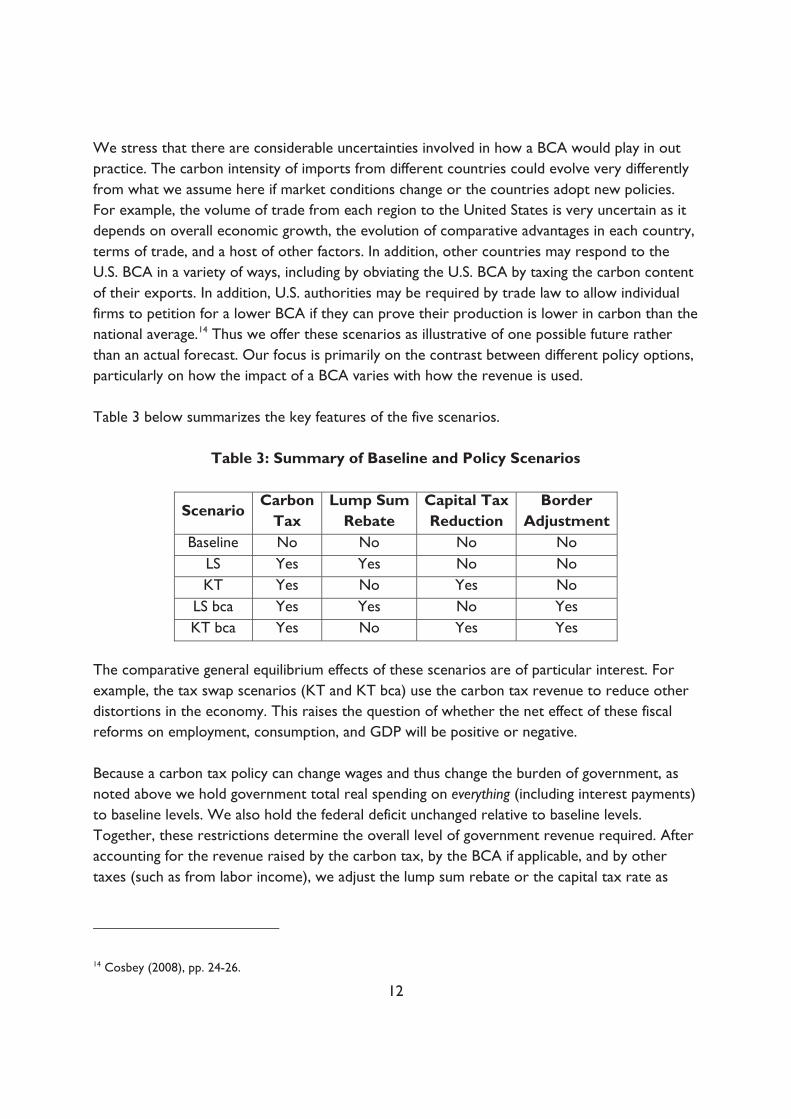
To put these figures in perspective, the revenues are shown as a percent of baseline GDP in Figure 6. In 2020, the carbon taxes without BCAs raise revenue equivalent to about 0.5 percent of GDP, which is roughly similar to the total for all U.S. federal excises taxes today.15 Through 2040, the increase in the carbon tax rate approximately balances out the decline in emissions. Revenue from BCAs adds about 0.25 percent of GDP in 2020 and grows to about 0.6 percent of GDP by 2040.
Figure 6: Gross Revenue as a Percent of Baseline GDP
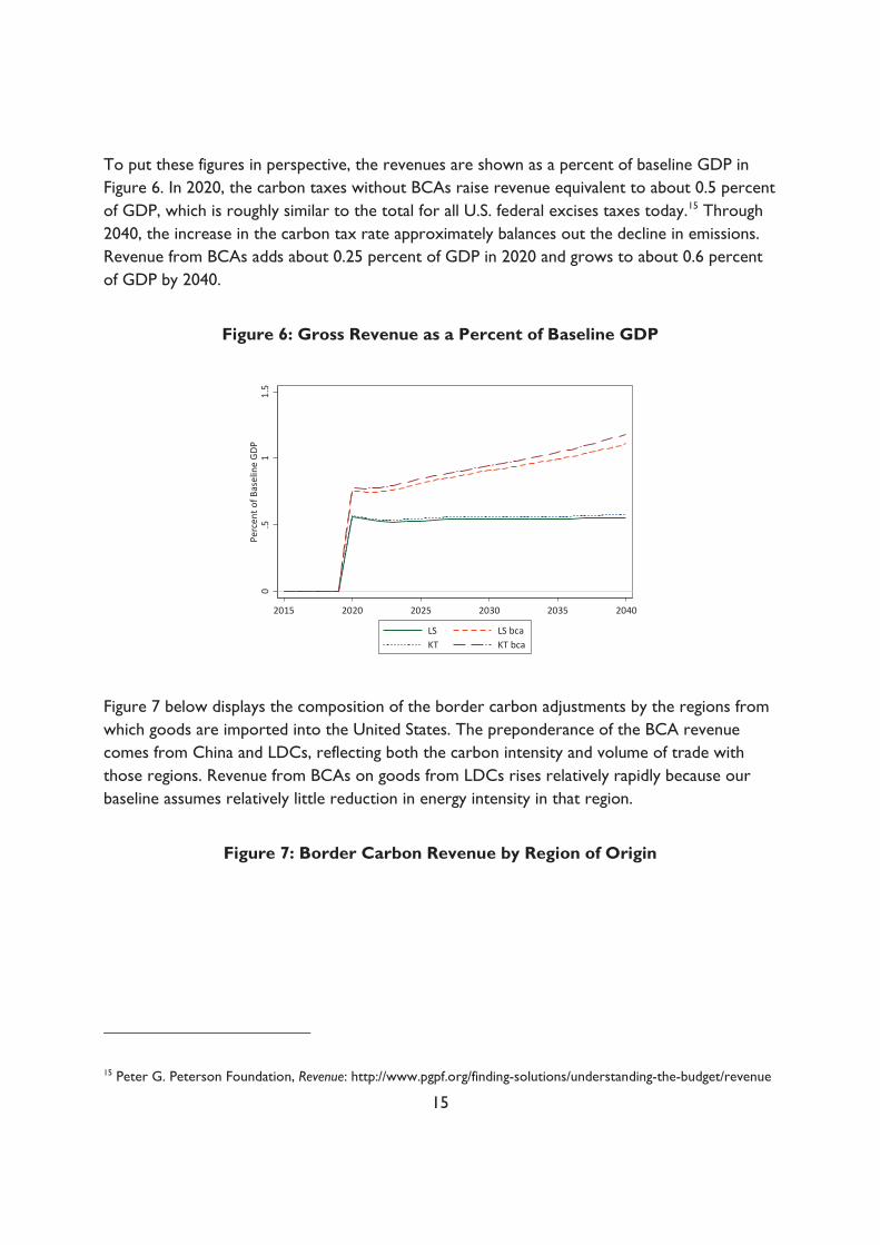
Figure 7 below displays the composition of the border carbon adjustments by the regions from which goods are imported into the United States. The preponderance of the BCA revenue comes from China and LDCs, reflecting both the carbon intensity and volume of trade with those regions. Revenue from BCAs on goods from LDCs rises relatively rapidly because our baseline assumes relatively little reduction in energy intensity in that region.
Figure 7: Border Carbon Revenue by Region of Origin
15 Peter G. Peterson Foundation, Revenue: http://www.pgpf.org/finding-solutions/understanding-the-budget/revenue
0.5
11.
5Pe
rcen
t of B
asel
ine
GDP
2015 2020 2025 2030 2035 2040
LS LS bcaKT KT bca
15
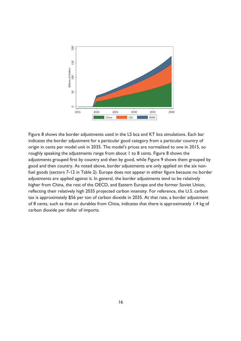
Figure 8 shows the border adjustments used in the LS bca and KT bca simulations. Each bar indicates the border adjustment for a particular good category from a particular country of origin in cents per model unit in 2035. The model’s prices are normalized to one in 2015, so roughly speaking the adjustments range from about 1 to 8 cents. Figure 8 shows the adjustments grouped first by country and then by good, while Figure 9 shows them grouped by good and then country. As noted above, border adjustments are only applied on the six non-fuel goods (sectors 7-12 in Table 2). Europe does not appear in either figure because no border adjustments are applied against it. In general, the border adjustments tend to be relatively higher from China, the rest of the OECD, and Eastern Europe and the former Soviet Union, reflecting their relatively high 2035 projected carbon intensity. For reference, the U.S. carbon tax is approximately $56 per ton of carbon dioxide in 2035. At that rate, a border adjustment of 8 cents, such as that on durables from China, indicates that there is approximately 1.4 kg of carbon dioxide per dollar of imports.
050
100
150
200
Billi
ons o
f Dol
lars
2015 2020 2025 2030 2035 2040
China LDC ROW
16
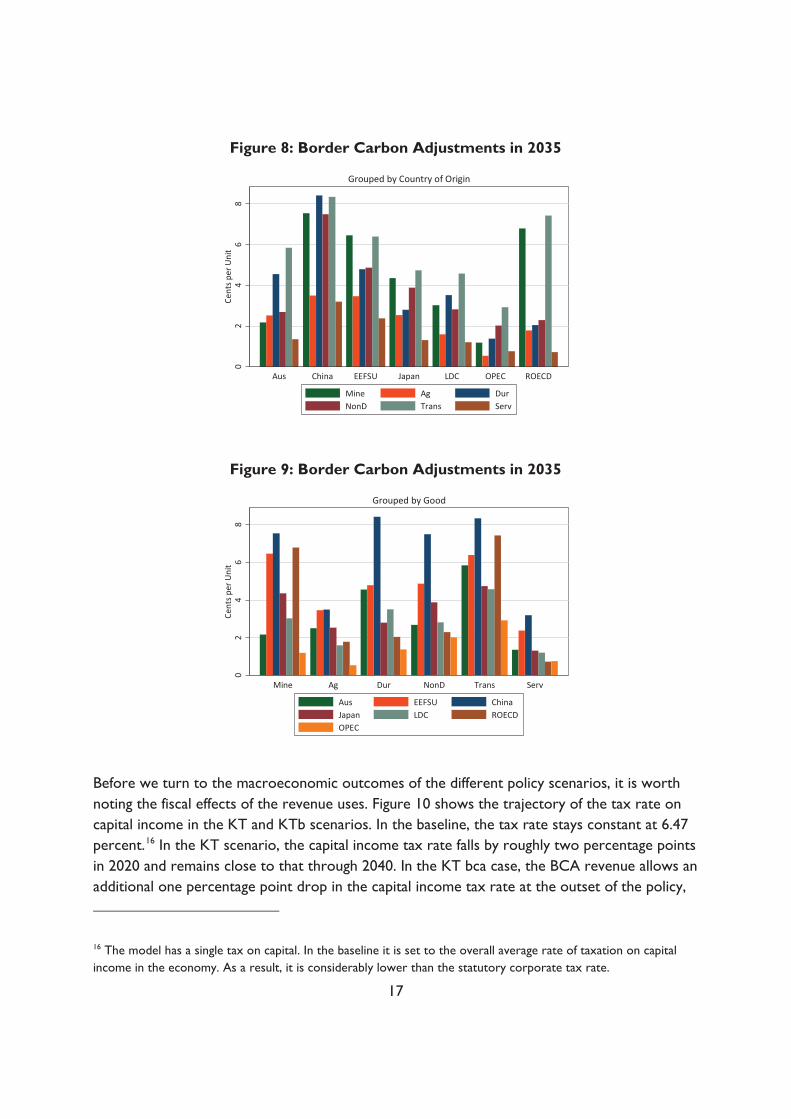
Figure 8: Border Carbon Adjustments in 2035
Figure 9: Border Carbon Adjustments in 2035
Before we turn to the macroeconomic outcomes of the different policy scenarios, it is worth noting the fiscal effects of the revenue uses. Figure 10 shows the trajectory of the tax rate on capital income in the KT and KTb scenarios. In the baseline, the tax rate stays constant at 6.47 percent.16 In the KT scenario, the capital income tax rate falls by roughly two percentage points in 2020 and remains close to that through 2040. In the KT bca case, the BCA revenue allows an additional one percentage point drop in the capital income tax rate at the outset of the policy,
16 The model has a single tax on capital. In the baseline it is set to the overall average rate of taxation on capital income in the economy. As a result, it is considerably lower than the statutory corporate tax rate.
02
46
8Ce
nts p
er U
nit
Aus China EEFSU Japan LDC OPEC ROECD
Grouped by Country of Origin
Mine Ag DurNonD Trans Serv
02
46
8Ce
nts p
er U
nit
Mine Ag Dur NonD Trans Serv
Grouped by Good
Aus EEFSU ChinaJapan LDC ROECDOPEC
17

and by 2040 the capital income tax rate is down to a little less than one percent, a 5.6 percentage point drop from its baseline level.
Figure 10: Capital Income Tax Rate
Figure 11 shows levels of real U.S. GDP for all the scenarios. We see that none of the carbon tax policies cause GDP to fall in absolute terms; rather, they cause a very slight slowing in GDP growth. Indeed, generally the United States achieves the same level of GDP in the policy scenarios only a few months after it does in the no-policy baseline. We emphasize this point here, because in other figures below we report changes relative to baseline. While the differences may look dramatic, a careful reading of the vertical axes indicates that many policy effects are less than a percentage point or two of those same outcomes in the baseline case. Recall as well that we are not accounting for the potential economic benefits of the climatic damages avoided.
02
46
Rate
2015 2020 2025 2030 2035 2040
Base KT KT bca
18
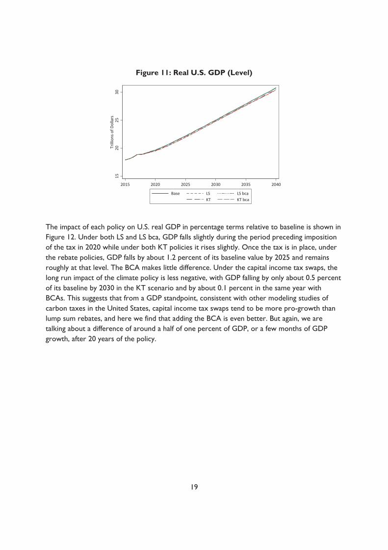
Figure 11: Real U.S. GDP (Level)
The impact of each policy on U.S. real GDP in percentage terms relative to baseline is shown in Figure 12. Under both LS and LS bca, GDP falls slightly during the period preceding imposition of the tax in 2020 while under both KT policies it rises slightly. Once the tax is in place, under the rebate policies, GDP falls by about 1.2 percent of its baseline value by 2025 and remains roughly at that level. The BCA makes little difference. Under the capital income tax swaps, the long run impact of the climate policy is less negative, with GDP falling by only about 0.5 percent of its baseline by 2030 in the KT scenario and by about 0.1 percent in the same year with BCAs. This suggests that from a GDP standpoint, consistent with other modeling studies of carbon taxes in the United States, capital income tax swaps tend to be more pro-growth than lump sum rebates, and here we find that adding the BCA is even better. But again, we are talking about a difference of around a half of one percent of GDP, or a few months of GDP growth, after 20 years of the policy.
1520
2530
Trill
ions
of D
olla
rs
2015 2020 2025 2030 2035 2040
Base LS LS bcaKT KT bca
19
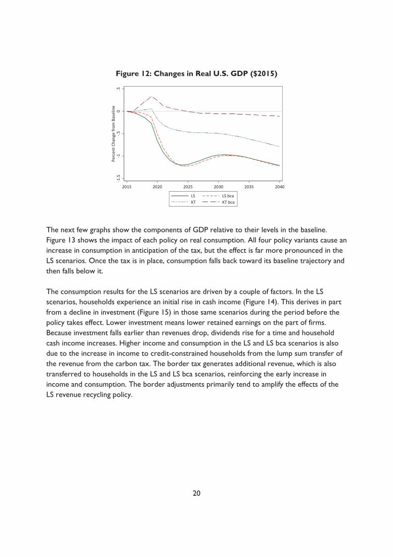
Figure 12: Changes in Real U.S. GDP ($2015)
The next few graphs show the components of GDP relative to their levels in the baseline. Figure 13 shows the impact of each policy on real consumption. All four policy variants cause an increase in consumption in anticipation of the tax, but the effect is far more pronounced in the LS scenarios. Once the tax is in place, consumption falls back toward its baseline trajectory and then falls below it. The consumption results for the LS scenarios are driven by a couple of factors. In the LS scenarios, households experience an initial rise in cash income (Figure 14). This derives in part from a decline in investment (Figure 15) in those same scenarios during the period before the policy takes effect. Lower investment means lower retained earnings on the part of firms. Because investment falls earlier than revenues drop, dividends rise for a time and household cash income increases. Higher income and consumption in the LS and LS bca scenarios is also due to the increase in income to credit-constrained households from the lump sum transfer of the revenue from the carbon tax. The border tax generates additional revenue, which is also transferred to households in the LS and LS bca scenarios, reinforcing the early increase in income and consumption. The border adjustments primarily tend to amplify the effects of the LS revenue recycling policy.
-1.5
-1-.5
0.5
Perc
ent C
hang
e fr
om B
asel
ine
2015 2020 2025 2030 2035 2040
LS LS bcaKT KT bca
20
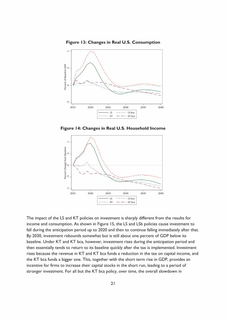
Figure 13: Changes in Real U.S. Consumption
Figure 14: Changes in Real U.S. Household Income
The impact of the LS and KT policies on investment is sharply different from the results for income and consumption. As shown in Figure 15, the LS and LSb policies cause investment to fall during the anticipation period up to 2020 and then to continue falling immediately after that. By 2030, investment rebounds somewhat but is still about one percent of GDP below its baseline. Under KT and KT bca, however, investment rises during the anticipation period and then essentially tends to return to its baseline quickly after the tax is implemented. Investment rises because the revenue in KT and KT bca funds a reduction in the tax on capital income, and the KT bca funds a bigger one. This, together with the short term rise in GDP, provides an incentive for firms to increase their capital stocks in the short run, leading to a period of stronger investment. For all but the KT bca policy, over time, the overall slowdown in
-.50
.51
Perc
ent o
f Bas
elin
e GD
P
2015 2020 2025 2030 2035 2040
LS LS bcaKT KT bca
-1-.5
0.5
1Pe
rcen
t Cha
nge
from
Bas
elin
e
2015 2020 2025 2030 2035 2040
LS LS bcaKT KT bca
21
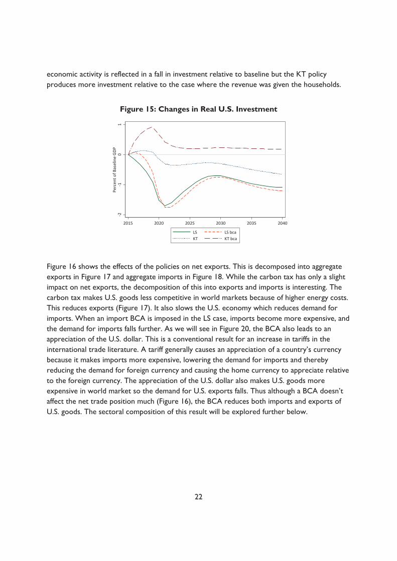
economic activity is reflected in a fall in investment relative to baseline but the KT policy produces more investment relative to the case where the revenue was given the households.
Figure 15: Changes in Real U.S. Investment
Figure 16 shows the effects of the policies on net exports. This is decomposed into aggregate exports in Figure 17 and aggregate imports in Figure 18. While the carbon tax has only a slight impact on net exports, the decomposition of this into exports and imports is interesting. The carbon tax makes U.S. goods less competitive in world markets because of higher energy costs. This reduces exports (Figure 17). It also slows the U.S. economy which reduces demand for imports. When an import BCA is imposed in the LS case, imports become more expensive, and the demand for imports falls further. As we will see in Figure 20, the BCA also leads to an appreciation of the U.S. dollar. This is a conventional result for an increase in tariffs in the international trade literature. A tariff generally causes an appreciation of a country’s currency because it makes imports more expensive, lowering the demand for imports and thereby reducing the demand for foreign currency and causing the home currency to appreciate relative to the foreign currency. The appreciation of the U.S. dollar also makes U.S. goods more expensive in world market so the demand for U.S. exports falls. Thus although a BCA doesn’t affect the net trade position much (Figure 16), the BCA reduces both imports and exports of U.S. goods. The sectoral composition of this result will be explored further below.
-2-1
01
Perc
ent o
f Bas
elin
e GD
P
2015 2020 2025 2030 2035 2040
LS LS bcaKT KT bca
22
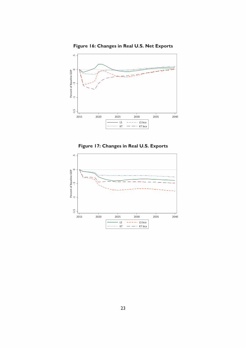
Figure 16: Changes in Real U.S. Net Exports
Figure 17: Changes in Real U.S. Exports
-1.5
-1-.5
0.5
Perc
ent o
f Bas
elin
e GD
P
2015 2020 2025 2030 2035 2040
LS LS bcaKT KT bca
-1.5
-1-.5
0.5
Perc
ent o
f Bas
elin
e G
DP
2015 2020 2025 2030 2035 2040
LS LS bcaKT KT bca
23

Figure 18: Changes in Real U.S. Imports
The changes in real interest rates and the real exchange rate appear in Figure 19 and Figure 20, respectively. The policies have little effect on U.S. interest rates. All four of the policies tend to appreciate the U.S. real exchange rate modestly right away, in anticipation of the policy, and then appreciate it further in the longer run. The appreciation reflects the assumption in the model that goods from different countries are imperfect substitutes. With a permanent fall in U.S. production, and the assumption that consumers demand goods from all countries, there is a rise in the relative price of U.S. goods in the global economy. To the extent that U.S. goods are more substitutable for goods from other countries, this effect will be smaller. The BCA reduces the relative price of U.S. goods in world markets which leads to a rise in demand for these goods and therefore in the demand for U.S. dollars to pay for them. Therefore, in equilibrium the U.S. real exchange rate has to appreciate further to clear the market. The LS policy causes a larger appreciation of the real exchange rate than the KT policy because the transfer raises household income, and therefore the demand for U.S. goods, which drives up prices. The KT policy, although also increasing demand for U.S. goods, increases the supply of U.S. goods over time through greater investment. Thus the price of U.S. goods relative to foreign goods (the real exchange rate) rises by more under the LS policy than the KT policy.
-1.5
-1-.5
0.5
Perc
ent o
f Bas
elin
e G
DP
2015 2020 2025 2030 2035 2040
LS LS bcaKT KT bca
24

Figure 19: Levels of the Real U.S. Interest Rate
Figure 20: Changes in Real Effective Exchange Rate of U.S. Dollar
The effect of the two policies on real wages is shown in Figure 21. Real wages fall relative to the baseline (although the baseline itself is rising) under each carbon tax scenario except KT bca. The carbon tax reduces the marginal product of capital, which drives down real wages. We find that only in the KS case does the BCA protect U.S. workers from the effects of a carbon tax.
-1-.5
0.5
11.
5Pe
rcen
t
2015 2020 2025 2030 2035 2040
Base LS LS bcaKT KT bca
01
23
45
Perc
ent C
hang
e fr
om B
asel
ine
2015 2020 2025 2030 2035 2040
Base LS LS bcaKT KT bca
25
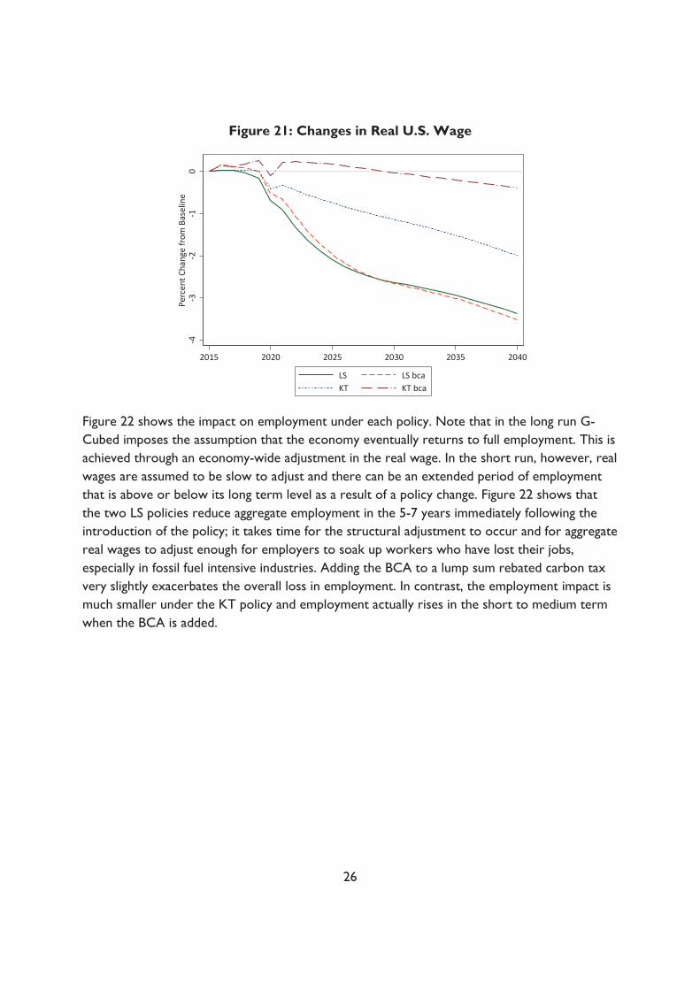
Figure 21: Changes in Real U.S. Wage
Figure 22 shows the impact on employment under each policy. Note that in the long run G-Cubed imposes the assumption that the economy eventually returns to full employment. This is achieved through an economy-wide adjustment in the real wage. In the short run, however, real wages are assumed to be slow to adjust and there can be an extended period of employment that is above or below its long term level as a result of a policy change. Figure 22 shows that the two LS policies reduce aggregate employment in the 5-7 years immediately following the introduction of the policy; it takes time for the structural adjustment to occur and for aggregate real wages to adjust enough for employers to soak up workers who have lost their jobs, especially in fossil fuel intensive industries. Adding the BCA to a lump sum rebated carbon tax very slightly exacerbates the overall loss in employment. In contrast, the employment impact is much smaller under the KT policy and employment actually rises in the short to medium term when the BCA is added.
-4-3
-2-1
0Pe
rcen
t Cha
nge
from
Bas
elin
e
2015 2020 2025 2030 2035 2040
LS LS bcaKT KT bca
26
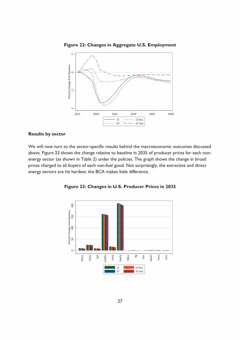
Figure 22: Changes in Aggregate U.S. Employment
Results by sector We will now turn to the sector-specific results behind the macroeconomic outcomes discussed above. Figure 23 shows the change relative to baseline in 2035 of producer prices for each non-energy sector (as shown in Table 2) under the policies. The graph shows the change in broad prices charged to all buyers of each non-fuel good. Not surprisingly, the extractive and direct energy sectors are hit hardest; the BCA makes little difference.
Figure 23: Changes in U.S. Producer Prices in 2035
-1-.5
0.5
Perc
ent C
hang
e fr
om B
asel
ine
2015 2020 2025 2030 2035 2040
LS LS bcaKT KT bca
050
100
150
200
Perc
ent C
hang
e fr
om B
asel
ine
Elec
U
Gas
U
Ref
Coal
Ex
CrO
il
Gas
Ex
Min
e Ag Dur
Non
D
Tran
s
Serv
LS LS bcaKT KT bca
27
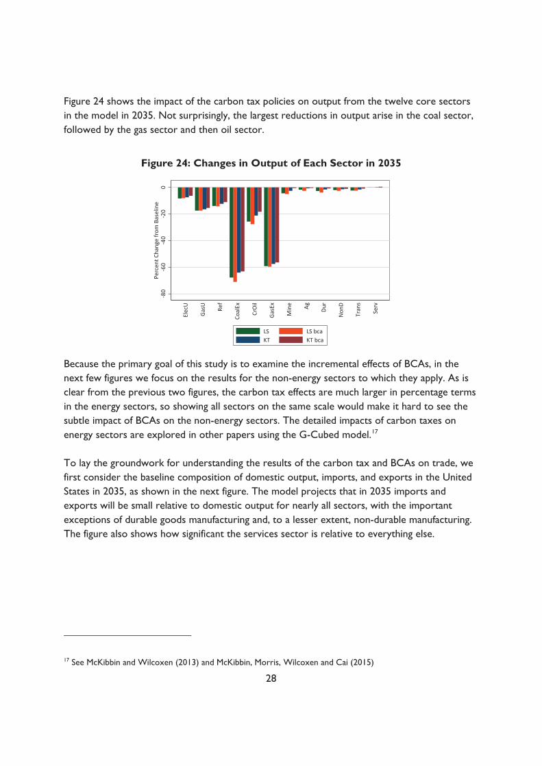
Figure 24 shows the impact of the carbon tax policies on output from the twelve core sectors in the model in 2035. Not surprisingly, the largest reductions in output arise in the coal sector, followed by the gas sector and then oil sector.
Figure 24: Changes in Output of Each Sector in 2035
Because the primary goal of this study is to examine the incremental effects of BCAs, in the next few figures we focus on the results for the non-energy sectors to which they apply. As is clear from the previous two figures, the carbon tax effects are much larger in percentage terms in the energy sectors, so showing all sectors on the same scale would make it hard to see the subtle impact of BCAs on the non-energy sectors. The detailed impacts of carbon taxes on energy sectors are explored in other papers using the G-Cubed model.17 To lay the groundwork for understanding the results of the carbon tax and BCAs on trade, we first consider the baseline composition of domestic output, imports, and exports in the United States in 2035, as shown in the next figure. The model projects that in 2035 imports and exports will be small relative to domestic output for nearly all sectors, with the important exceptions of durable goods manufacturing and, to a lesser extent, non-durable manufacturing. The figure also shows how significant the services sector is relative to everything else.
17 See McKibbin and Wilcoxen (2013) and McKibbin, Morris, Wilcoxen and Cai (2015)
-80
-60
-40
-20
0Pe
rcen
t Cha
nge
from
Bas
elin
e
Elec
U
Gas
U
Ref
Coal
Ex
CrO
il
Gas
Ex
Min
e Ag Dur
Non
D
Tran
s
Serv
LS LS bcaKT KT bca
28
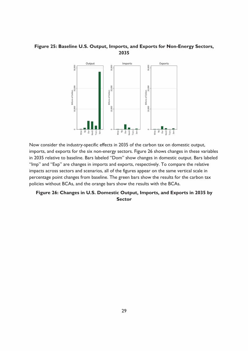
Figure 25: Baseline U.S. Output, Imports, and Exports for Non-Energy Sectors, 2035
Now consider the industry-specific effects in 2035 of the carbon tax on domestic output, imports, and exports for the six non-energy sectors. Figure 26 shows changes in these variables in 2035 relative to baseline. Bars labeled “Dom” show changes in domestic output. Bars labeled “Imp” and “Exp” are changes in imports and exports, respectively. To compare the relative impacts across sectors and scenarios, all of the figures appear on the same vertical scale in percentage point changes from baseline. The green bars show the results for the carbon tax policies without BCAs, and the orange bars show the results with the BCAs.
Figure 26: Changes in U.S. Domestic Output, Imports, and Exports in 2035 by Sector
010
,000
20,0
0030
,000
Billi
ons o
f Dol
lars
Min
e Ag Dur
Non
D
Tran
s
Serv
Output
010
,000
20,0
0030
,000
Billi
ons o
f Dol
lars
Min
e Ag Dur
Non
D
Tran
s
Serv
Imports
010
,000
20,0
0030
,000
Billi
ons o
f Dol
lars
Min
e Ag Dur
Non
D
Tran
s
Serv
Exports
29
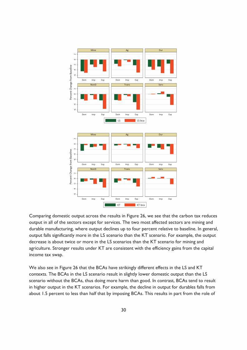
Comparing domestic output across the results in Figure 26, we see that the carbon tax reduces output in all of the sectors except for services. The two most affected sectors are mining and durable manufacturing, where output declines up to four percent relative to baseline. In general, output falls significantly more in the LS scenario than the KT scenario. For example, the output decrease is about twice or more in the LS scenarios than the KT scenario for mining and agriculture. Stronger results under KT are consistent with the efficiency gains from the capital income tax swap. We also see in Figure 26 that the BCAs have strikingly different effects in the LS and KT contexts. The BCAs in the LS scenario result in slightly lower domestic output than the LS scenario without the BCAs, thus doing more harm than good. In contrast, BCAs tend to result in higher output in the KT scenarios. For example, the decline in output for durables falls from about 1.5 percent to less than half that by imposing BCAs. This results in part from the role of
-6-4
-20
2-6
-4-2
02
Dom Imp Exp Dom Imp Exp Dom Imp Exp
Dom Imp Exp Dom Imp Exp Dom Imp Exp
Mine Ag Dur
NonD Trans Serv
KT KT bca
Perc
ent C
hang
e fr
om B
asel
ine
-6-4
-20
2-6
-4-2
02
Dom Imp Exp Dom Imp Exp Dom Imp Exp
Dom Imp Exp Dom Imp Exp Dom Imp Exp
Mine Ag Dur
NonD Trans Serv
LS LS bca
Perc
ent C
hang
e fr
om B
asel
ine
30

the additional revenue from the BCAs in further reducing the tax rate on capital income, as shown in Figure 10. Recall that Figure 18 showed no evidence of an economy-wide surge in imports upon the imposition of the carbon tax. Figure 26 shows that the same is true in all of individual sectors. Thus, at the level of the broad categories of economic activity in the model, we see no evidence of a broad competitiveness problem. Of course, trade in individual subsectors (that is, in narrower segments of the economy than the sectors in the model) may be far more sensitive. We saw in Figure 16 that overall net exports across the U.S. economy are lower than baseline in the carbon tax scenarios. Consistent with that, we see in Figure 26 that in most sectors in percentage terms exports fall by more than imports, particularly in the scenarios with the BCAs and particularly for the LS scenarios. Thus, if policymakers are concerned about net exports from the United States, it may be preferable to impose a carbon tax with no border adjustments than a carbon tax with BCAs only on imports. Next consider the politically-important durable goods manufacturing sector in more detail. In the LS and KT scenarios, the carbon tax lowers domestic production by roughly the same proportion as it lowers imports. That means that to the extent that the carbon tax reduces the market for durables, it doesn’t not disproportionately disadvantage domestic durables relative to imported durables. In both the LS and KT scenarios without BCAs, imports fall a little more than exports, but both fall more in the LS scenario. With BCAs, the capital income tax swap scenario reduces exports far more than imports, whereas with rebates the two percentage changes are about the same. These outcomes are an amalgam of several competing factors, in addition to the shift in the relative costs of production in the United States and abroad that results from the carbon tax. First, as we saw in Figure 20, in general equilibrium the carbon tax induces a stronger U.S. dollar. That has a tendency to increase imports and lower exports. At the same time, in the LS scenarios the carbon tax drives overall economic activity in the United States, particularly investment (Figure 15), slightly below baseline, and that would tend to lower both imports and domestic output, all else equal. Finally, the carbon tax shifts the composition of goods and services produced and consumed in the U.S. economy, and that can affect domestic output and imports and exports. For example, the carbon tax shifts consumption towards relatively low-emissions-intensive services, which are disproportionately domestically produced. Overall, our results show that if policymakers want to minimize the impact on domestic output, it is more important to focus on choosing an efficient use of the revenue than on addressing trade competition.
31
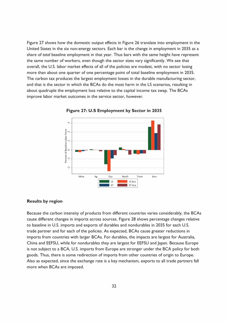
Figure 27 shows how the domestic output effects in Figure 26 translate into employment in the United States in the six non-energy sectors. Each bar is the change in employment in 2035 as a share of total baseline employment in that year. Thus bars with the same height have represent the same number of workers, even though the sector sizes vary significantly. We see that overall, the U.S. labor market effects of all of the policies are modest, with no sector losing more than about one quarter of one percentage point of total baseline employment in 2035. The carbon tax produces the largest employment losses in the durable manufacturing sector, and that is the sector in which the BCAs do the most harm in the LS scenarios, resulting in about quadruple the employment loss relative to the capital income tax swap. The BCAs improve labor market outcomes in the service sector, however.
Figure 27: U.S Employment by Sector in 2035
Results by region Because the carbon intensity of products from different countries varies considerably, the BCAs cause different changes in imports across sources. Figure 28 shows percentage changes relative to baseline in U.S. imports and exports of durables and nondurables in 2035 for each U.S. trade partner and for each of the policies. As expected, BCAs cause greater reductions in imports from countries with larger BCAs. For durables, the impacts are largest for Australia, China and EEFSU, while for nondurables they are largest for EEFSU and Japan. Because Europe is not subject to a BCA, U.S. imports from Europe are stronger under the BCA policy for both goods. Thus, there is some redirection of imports from other countries of origin to Europe. Also as expected, since the exchange rate is a key mechanism, exports to all trade partners fall more when BCAs are imposed.
-.2-.1
0.1
.2.3
Perc
ent o
f Bas
elin
e La
bor F
orce
Mine Ag Dur NonD Trans Serv
LS LS bcaKT KT bca
32
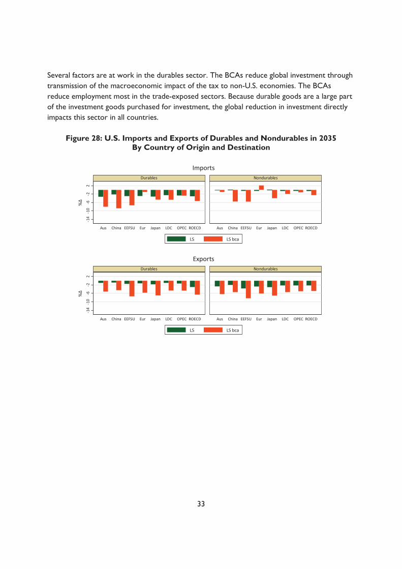
Several factors are at work in the durables sector. The BCAs reduce global investment through transmission of the macroeconomic impact of the tax to non-U.S. economies. The BCAs reduce employment most in the trade-exposed sectors. Because durable goods are a large part of the investment goods purchased for investment, the global reduction in investment directly impacts this sector in all countries.
Figure 28: U.S. Imports and Exports of Durables and Nondurables in 2035 By Country of Origin and Destination
-14
-10
-6-2
2
Aus China EEFSU Eur Japan LDC OPEC ROECD Aus China EEFSU Eur Japan LDC OPEC ROECD
Durables Nondurables
LS LS bca
Imports
-14
-10
-6-2
2
Aus China EEFSU Eur Japan LDC OPEC ROECD Aus China EEFSU Eur Japan LDC OPEC ROECD
Durables Nondurables
LS LS bca
Exports
33

As shown in Figure 29, U.S. policies cause changes in the real GDP of other regions. By 2035 real GDP falls slightly for most regions. Because there are no BCAs on imports from the E.U., GDP in the E.U. is very slightly higher reflecting a switch in world demand towards Europe as a result of the U.S. border carbon policy. The negative spillovers of the carbon policies are largest for OPEC and ROECD (which in G-Cubed is mostly Canada). The BCAs accentuate the spillovers for all regions except for ROECD.
Figure 29: Impacts on Real GDP by Region in 2035
-14
-10
-6-2
2
Aus China EEFSU Eur Japan LDC OPEC ROECD Aus China EEFSU Eur Japan LDC OPEC ROECD
Durables Nondurables
KT KT bca
Imports-1
4-1
0-6
-22
Aus China EEFSU Eur Japan LDC OPEC ROECD Aus China EEFSU Eur Japan LDC OPEC ROECD
Durables Nondurables
KT KT bca
Exports
-1-.8
-.6-.4
-.20
Perc
ent C
hang
e fr
om B
asel
ine
Aus China EEFSU Eur Japan LDC OPEC ROECD USA
LS LS bcaKT KT bca
34
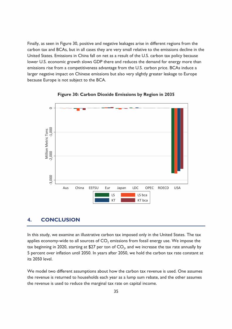
Finally, as seen in Figure 30, positive and negative leakages arise in different regions from the carbon tax and BCAs, but in all cases they are very small relative to the emissions decline in the United States. Emissions in China fall on net as a result of the U.S. carbon tax policy because lower U.S. economic growth slows GDP there and reduces the demand for energy more than emissions rise from a competitiveness advantage from the U.S. carbon price. BCAs induce a larger negative impact on Chinese emissions but also very slightly greater leakage to Europe because Europe is not subject to the BCA.
Figure 30: Carbon Dioxide Emissions by Region in 2035
4. CONCLUSION
In this study, we examine an illustrative carbon tax imposed only in the United States. The tax applies economy-wide to all sources of CO2 emissions from fossil energy use. We impose the tax beginning in 2020, starting at $27 per ton of CO2, and we increase the tax rate annually by 5 percent over inflation until 2050. In years after 2050, we hold the carbon tax rate constant at its 2050 level. We model two different assumptions about how the carbon tax revenue is used. One assumes the revenue is returned to households each year as a lump sum rebate, and the other assumes the revenue is used to reduce the marginal tax rate on capital income.
-3,0
00-2
,000
-1,0
000
Mill
ion
Met
ric T
ons
Aus China EEFSU Eur Japan LDC OPEC ROECD USA
LS LS bcaKT KT bca
35

We also run a variation on each policy in which import BCAs are imposed to account for the total embodied carbon in each non-fuel import from each country of origin other than Europe. The revenue from the BCAs is returned to households or firms according to the same assumptions as the core policies. We treat European goods as exempt from border adjustments on the grounds Europe has adopted policies that are very roughly comparable to the tax being imposed in the United States. Consistent with earlier studies, we find that the carbon tax raises considerable revenue and reduces CO2 emissions significantly relative to baseline, no matter how the revenue is used. Gross annual revenue from the carbon tax with lump sum rebating and no BCA begins at $110 billion in 2020 and rises gradually to $170 billion in 2040. By 2040, annual CO2 emissions fall from 5.5 billion metric tons (BMT) under the baseline to 2.4 BMT, a decline of 3.1 BMT, or 57 percent. Cumulative emissions over 2020 to 2040 fall by 48 BMT. Also consistent with earlier studies, we find that the carbon tax has very small overall impacts on GDP, wages, employment, and consumption. Different uses of the revenue from the carbon tax result in slightly different levels and compositions of GDP across consumption, investment and net exports. Overall, using carbon tax revenue to reduce the capital income tax rate results in better macroeconomic outcomes than using the revenue for lump sum transfers. Indeed, even while achieving remarkable emissions reductions, the policy results in the U.S. economy reaching the output projections in 2040 only about three months later than it would without the carbon tax. The G-Cubed model is uniquely suited to investigating the effects of these policy scenarios on emissions leakage, trade, and investment flows. We find no evidence of significant leakage. If anything, the slight slowing of the U.S. economy and demand for imports result in lower emissions abroad. We find that the carbon tax increases the input price of energy, which lowers U.S. exports and slows the U.S. economy, which in turn reduces demand for imports. When an import BCA is imposed, imports become more expensive, and the demand for imports falls further. The BCA also leads to a conventional result from the international trade literature for an increase in tariffs: the U.S. dollar strengthens. A tariff generally causes an appreciation of a country’s currency: as the demand for imports falls, the demand for foreign currency falls, which strengthens the home currency relative to the foreign currency. The appreciation of the U.S. dollar also makes U.S. goods more expensive in world market so the demand for U.S. exports falls. Thus although a BCA doesn’t affect the U.S. net trade position much, it reduces both imports and exports of U.S. goods. While the intent of BCAs is to protect U.S. workers from the effects of a carbon tax, we find they can actually have the opposite result, depending on how the revenues are used. To our
36

knowledge, this is the first study to identify the potential linkages between the effect of a BCA and the use of carbon tax revenue. In the lump sum rebate scenarios, the BCAs reduce employment most in the trade-exposed sectors. The largest effect is on durable manufacturing. This is partly a price effect from the stronger U.S. dollar, but it is also because the BCAs reduce global investment through transmission of the macroeconomic impact of the carbon tax to non-U.S. economies. Because durable goods are a large part of the goods purchased for investment, the global reduction in investment directly impacts this sector in all countries. In the capital tax swap scenarios, the BCAs generally improve U.S. employment outcomes, including in trade-exposed sectors. Future work could extend the analysis to include a border carbon adjustment on exports. Such a policy would provide rebates to U.S. exporters of the carbon taxes paid during production of their goods. The overall impact of an export BCA would depend on the interaction of the similar factors to those discussed above for the import BCA. There would be a price effect as the export BCA lowers the price of energy-intensive exports, which would tend to raise demand, and hence production, of those goods. However, the export BCA would also lower the amount of revenue available for a lump sum rebate or a reduction in the capital tax rate, hence reducing output through macroeconomic reductions in demand. Finally, making U.S. exports more attractive would tend to strengthen the U.S. dollar, partially offsetting the price effect for energy-intensive exports and reducing demand for non-energy-intensive exports. In sum, a carefully designed carbon tax in the United States can reduce emissions significantly with minimal effect on the economy. We find no evidence of meaningful emissions leakage abroad, even when the U.S. policy is unilateral. Using carbon tax and BCA revenue to reduce distortionary taxes produces better economic outcomes overall and for most individual sectors. To the extent that policymakers wish to protect the interests of energy-intensive trade-exposed industries with BCAs on imports, they should endeavor to tailor the adjustments to narrow, particularly vulnerable, subsectors so as not to inadvertently appreciate the U.S. dollar and do more harm than good overall.
37
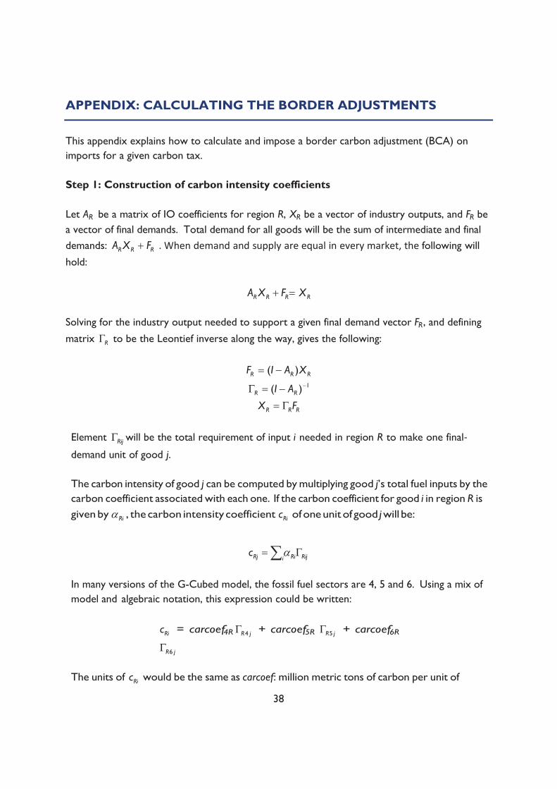
APPENDIX: CALCULATING THE BORDER ADJUSTMENTS
This appendix explains how to calculate and impose a border carbon adjustment (BCA) on imports for a given carbon tax. Step 1: Construction of carbon intensity coefficients Let AR be a matrix of IO coefficients for region R, XR be a vector of industry outputs, and FR be a vector of final demands. Total demand for all goods will be the sum of intermediate and final demands: RRR FXA . When demand and supply are equal in every market, the following will
hold:
RRRR XFXA
Solving for the industry output needed to support a given final demand vector FR , and defining
matrix R to be the Leontief inverse along the way, gives the following:
RRR XAIF )( 1)( RR AI
RRR FX Element Rij will be the total requirement of input i needed in region R to make one final- demand unit of good j.
The carbon intensity of good j can be computed by multiplying good j’s total fuel inputs by the carbon coefficient associated with each one. If the carbon coefficient for good i in region R is given by Ri , the carbon intensity coefficient Ric of one unit of good j will be:
i RijRiRjc
In many versions of the G-Cubed model, the fossil fuel sectors are 4, 5 and 6. Using a mix of model and algebraic notation, this expression could be written:
Ric = carcoef4R jR4 + carcoef5R jR5 + carcoef6R
jR6
The units of Ric would be the same as carcoef: million metric tons of carbon per unit of
38

model output. As an example, the vector of intensities for China in G-Cubed is shown in Table A1. Note that the coefficients for sectors 2-6 are omitted because they are fossil fuels and imports are taxed directly (no need for border adjustments). Coefficients for sectors 1 and 13-20 are also omitted since they are delivered or generated electricity and are essentially non-traded.
Table A1. Carbon Intensity Coefficients for China in G--Cubed
Sector j Ric , mmt C per unit of output
7 0.00038 8 0.00010 9 0.00011 10 0.00013 11 0.00042 12 0.00004
Step 2: Construct BCAs
Now suppose that country A imposes carbon tax TCARA on domestic production and imports of fossil fuels, and that country B does not have a similar tax. If A wants to impose a border carbon tax on imports from country B it would like to charge the following on good j imported to A from B:
ABiABj TCARcBCT
Step 3: Compute revenue from BCAs
The externality revenue in destination country A is increased by the following, where j ranges over traded goods and B ranges over countries of origin:
j B jABABjIMPBCT
An equivalent computation that may be more convenient for some purposes would be to compute the total embodied carbon in imports by country A (denoted ECARA) and then multiply by the tax:
j B jABBjA IMPcECAR
The revenue is then:
39

TCARAECARA
REFERENCES Aldy, Joseph E., and William Pizer. 2009. The Competitiveness Impacts of Climate Change Mitigation Policies. Arlington, VA: Center for Climate and Energy Solutions. http://www.c2es.org/docUploads/competitiveness-impacts-report.pdf. Böhringer, Christoph, Jared Carbone, and Thomas Rutherford. 2012. “Unilateral Climate Policy Design: Efficiency and Equity Implications of Alternative Instruments to Reduce Carbon Leakage.” Energy Economics: Supplement 2. 34: S208– S217. http://dx.doi.org/10.1016/j.eneco.2012.09.011. Branger, Frédéric, and Philippe Quirion. 2014. “Would Border Carbon Adjustments Prevent
Carbon Leakage and Heavy Industry Competitiveness Losses? Insights from a Meta-analysis of Recent Economic Studies.” Ecological Economics 99: 29–39. http://dx.doi.org/10.1016/j.ecolecon.2013.12.010.
Congressional Budget Office. 2011. Reducing the Deficit: Spending and Revenue Options. Washington, DC: Congressional Budget Office. http://www.cbo.gov/publication/22043. Congressional Budget Office. 2013. Border Adjustments for Economy-wide Policies That Impose a
Price on Greenhouse Gas Emissions. Washington, DC: Congressional Budget Office. https://www.cbo.gov/sites/default/files/113th-congress-2013-2014/reports/44971-GHGandTrade.pdf.
Condon, Madison, and Ada Ignaciuk. 2013. Border Carbon Adjustment and International Trade: A Literature Review. Paris: Organization for Economic Cooperation and Development Trade and Environment Working Papers. http://dx.doi.org/10.1787/5k3xn25b386c-en. Cosbey, Aaron. 2008. Border Carbon Adjustment. Winnipeg: International Institute for Sustainable Development. https://www.iisd.org/pdf/2008/cph_trade_climate_border_carbon.pdf. Elmendorf, Douglas W., 2009. Statement to the U.S. Senate Committee on Finance, The
Distribution of Revenues from a Cap-and-Trade Program for CO2 Emissions: Hearing before the Committee on Finance, 111th Cong., 1st sess., May 7, 2009. Washington: U.S. G.P.O. https://www.cbo.gov/sites/default/files/111th-congress-2009-2010/reports/05-07-cap_and_trade_testimony.pdf.
40
Fischer, Carolyn, and Alan K. Fox. 2012a. “Climate Policy and Fiscal Constraints: Do Tax Interactions Outweigh Carbon Leakage?” Energy Economics: Supplement 2. 34: S218-S227. http://dx.doi.org/10.1016/j.eneco.2012.09.004. Fischer, Carolyn, and Alan K. Fox. 2012b. “Comparing Policies to Combat Emissions Leakage: Border Tax Adjustments versus Rebates.” Journal of Environmental Economics and Management 64, no. 2: 199-216. http://dx.doi.org/10.2139/ssrn.1345928. Fischer, Carolyn, Richard Morgenstern, and Nathan Richardson. 2015. “Carbon Taxes and Energy-Intensive Trade-Exposed Industries”. Implementing A US Carbon Tax. Ian Parry, Adele C. Morris and Roberton C. Williams III. New York: Routledge, 2015. 159-177. Goulder, Lawrence H., 1995. “Environmental Taxation and the Double Taxation: A Reader’s Guide.” International Tax and Public Finance 2, no. 2: 157-183. http://dx.doi.org/10.1007/BF00877495. Jorgenson Dale W., Richard J. Goettle, Mun S. Ho, and Peter J. Wilcoxen. 2013. Double Dividend: Environmental Taxes and Fiscal Reform in the United States. MIT Press. https://doi.org/10.7551/mitpress/9780262027090.001.0001. Jorgenson, Dale W., Richard J Goettle, Mun S. Ho, and Peter J. Wilcoxen. 2015. “Carbon Taxes and Fiscal Reform in the United States.” National Tax Journal 68, no. 1: 121-138. http://dx.doi.org/10.17310/ntj.2015.1.05. Kortum, Samuel S., and David A. Weisbach. 2016. Border Adjustments for Carbon Emissions: Basic Concepts and Design. Discussion Paper RFF DP 16-09. Washington, DC: Resources for the Future. http://www.rff.org/files/document/file/RFF-DP-16-09.pdf. McKibbin, Warwick J., Adele C. Morris, and Peter J. Wilcoxen. 2012a. Pricing Carbon in the
United States: A Model-Based Analysis of Power Sector Only Approaches. Resource and Energy Economics 36 (2014) 130-150. http://www.brookings.edu/~/media/research/files/papers/2012/10/05-pricing-carbon-morris/05-pricingcarbon-morris.pdf.
McKibbin, Warwick J., Adele C. Morris, Peter J. Wilcoxen, and Yiyong Cai. 2012b. The Potential Role of a Carbon
https://www.brookings.edu/wp-content/uploads/2016/06/carbon-tax-mckibbin-morris-wilcoxen.pdf
41
McKibbin, Warwick J., Adele C. Morris, Peter J. Wilcoxen, and Yiyong Cai. 2015. “Carbon taxes and U.S. Fiscal Reform.” The National Tax Journal 68, no. 1: 139-156. http://dx.doi.org/10.17310/ntj.2015.1.06. McKibbin, Warwick J., David Pearce, and Alison Stegman. 2009. “Climate Change Scenarios and Long Term Projections.” Climate Change 97, no. 1: 23-47. http://dx.doi.org/10.1007/s10584-009-9621-3. McKibbin, Warwick J., and Peter J. Wilcoxen. 1999. “The Theoretical and Empirical Structure of the G-Cubed Model.” Economic Modelling 16, no.1: 123-148. https://www.brookings.edu/wp-content/uploads/2016/06/bdp118.pdf. McKibbin, Warwick J., and Peter J. Wilcoxen. 2013. “A Global Approach to Energy and Environment: The G-Cubed Model.” Handbook of Computable General Equilibrium Modeling, Elsevier: 995-1068. Rausch, Sebastian, and John Reilly. 2015. “Carbon Taxes, Deficits, and Energy Policy Interactions.” National Tax Journal 68, no. 1: 157-178. http://dx.doi.org/10.17310/ntj.2015.1.07. Sakai, Marco, and John Barrett. 2016. “Border Carbon Adjustments: Addressing Emissions Embodied in Trade.” Energy Policy 92: 102-110. http://dx.doi.org/10.1016/j.enpol.2016.01.038. Trachtman, Joel P. 2016. “WTO Law Constraints on Border Tax Adjustment and Tax Credit Mechanisms to Reduce the Competitive Effects of Carbon Taxes.” Discussion Paper RFF DP 16-03. Washington, DC: Resources for the Future.
http://www.rff.org/research/publications/wto-law-constraints-border-taxadjustment-and-tax-credit-mechanisms-reduce
Tuladhar, Sugandha D., W. David Montgomery, and Noah Kaufman. 2015. “Environmental Policy for Fiscal Reform: Can a Carbon Tax Play a Role?” National Tax Journal 68, no.1: 179-194. http://dx.doi.org/10.17310/ntj.2015.1.08.
42