Embed Size (px)
Citation preview

LETTERS
The role of mentorship in protege performanceR. Dean Malmgren1,2, Julio M. Ottino1,3 & Luıs A. Nunes Amaral1,3,4
The role of mentorship in protege performance is a matter of import-ance to academic, business and governmental organizations.Although the benefits of mentorship for proteges, mentors and theirorganizations are apparent1–9, the extent to which proteges mimictheir mentors’ career choices and acquire their mentorship skills isunclear10–16. The importance of a science, technology, engineeringand mathematics workforce to economic growth and the role ofeffective mentorship in maintaining a ‘healthy’ such workforcedemand the study of the role of mentorship in academia. Here weinvestigate one aspect of mentor emulation by studying mentorshipfecundity—the number of proteges a mentor trains—using datafrom the Mathematics Genealogy Project17, which tracks the mentor-ship record of thousands of mathematicians over several centuries.We demonstrate that fecundity among academic mathematicians iscorrelated with other measures of academic success. We also findthat the average fecundity of mentors remains stable over 60 years ofrecorded mentorship. We further discover three significant correla-tions in mentorship fecundity. First, mentors with low mentorshipfecundities train proteges that go on to have mentorship fecundities37% higher than expected. Second, in the first third of their careers,mentors with high fecundities train proteges that go on to havefecundities 29% higher than expected. Finally, in the last third oftheir careers, mentors with high fecundities train proteges that go onto have fecundities 31% lower than expected.
A large literature supports the hypothesis that proteges and mentorsbenefit from the mentoring relationship1,2. Proteges that receive careercoaching and social support, for instance, are reportedly more likely tohave high performance ratings, a higher salary and receive promo-tions1,3. In return, mentors receive fulfilment not only by altruisticallyimproving the welfare of their proteges, but also by improving their ownwelfare4,5,10. Organizations benefit as well, because proteges are morelikely to be committed to their organization6,7 and to exhibit organiza-tional citizenship behaviour6. These benefits are not obtained onlythrough the traditional dyadic mentor–protege relationship, but alsothrough peer relationships that supplement protege development8,9.
The benefits of mentorship underscore the importance of under-standing how mentors were in turn trained to foster the developmentof outstanding mentors. It might be suspected that proteges learnmanagerial approaches and motivational techniques from their men-tors and, as a result, emulate their mentorship methodologies; thissuggests that outstanding mentors are trained by other outstandingmentors. This possibility is sometimes formalized as the rising-starhypothesis11,12; it postulates that mentors select up-and-coming pro-teges on the basic of their perceived ability and potential and pastperformance10,13,14, including promotion history and proactive careerbehaviours12. Rising-star proteges are reportedly more likely tointend to mentor, resulting in a ‘perpetual cycle’ of rising-star pro-teges that emulate their mentors by seeking other rising stars as theirproteges15.
However, there is conflicting evidence concerning the rising-starhypothesis16, so the extent to which proteges mimic their mentors
remains an open question. Indeed, we are unaware of any studies thatsystematically track mentorship success over the entire career of amentor, so the validity of the rising-star hypothesis has yet to be fullyexplored. Here we investigate whether proteges acquire the mentor-ship skills of their mentors, by studying mentorship fecundity, that is,the number of proteges that a mentor trains over the course of theircareer. This measure is advantageous as it directly measures an out-come of the mentorship process that is relevant to sustained mentor-ship, allowing us to quantify the degree to which mentor fecunditydetermines protege fecundity.
Scientific mentorship offers a unique opportunity to study thisquestion because there is a structured mentorship environmentbetween advisor and student that is, in principle, readily accessible18,19.We study a prototypical mentorship network collected from theMathematics Genealogy Project17, which aggregates the graduationdate, mentor and proteges of 114,666 mathematicians from as earlyas 1637. This database is unique in its scope and coverage, tracking thecareer-long mentorship record of a large population of mentors in asingle discipline (see the MPACT Project (http://ils.unc.edu/mpact/)for a smaller database of theses on information and library sciencesand references therein). From this information, we construct a net-work in which links are formed from a mentor to each of his k pro-teges, where k denotes mentorship fecundity. We focus here on the7,259 mathematicians who graduated between 1900 and 1960, becausetheir mentorship record is the most reliable (Methods).
Although the mentorship records gathered from the MathematicsGenealogy Project provide the most comprehensive data source avail-able for the study of academic performance throughout a mathemati-cian’s career, there are obviously other plausible metrics for evaluatingacademic performance20–22. We have also compared the mentorshipdata against a list of publications for 4,447 mathematicians and a list of269 inductees into the US National Academy of Sciences (NAS;Methods). We find that mentorship fecundity is much larger forNAS members than for non-NAS members (Fig. 1a). We further findthat the number of publications is strongly correlated with fecundity,regardless of whether or not a mathematician is an NAS member(Fig. 1b). These results demonstrate that although fecundity is not atypical measure of academic performance, it is closely related to othermeasures of academic success. Thus, even though our investigationconcerns how fecundity is correlated between mentor and protege, ourresults also address questions in the academic evaluation literatureconcerning the success of a mathematician.
We first investigate whether it is possible to predict the fecundity ofa mathematician by modelling the empirical fecundity distribution,p(kjt), as a function of graduation year, t. Considering that somemathematicians remain in academia throughout their careers whereasothers spend only a portion of their careers in academia, it might beexpected that there are two types of individual when it comes toacademic mentorship fecundity—‘haves’ and ‘have-nots’—in thesense that mathematicians from these types respectively have or havenot had the opportunity to mentor students throughout their career.
1Department of Chemical and Biological Engineering, Northwestern University, Evanston, Illinois 60208, USA. 2Datascope Analytics, Evanston, Illinois 60201, USA. 3NorthwesternInstitute on Complex Systems, Northwestern University, Evanston, Illinois 60208, USA. 4Howard Hughes Medical Institute, Northwestern University, Evanston, Illinois 60208, USA.
Vol 465 | 3 June 2010 | doi:10.1038/nature09040
622Macmillan Publishers Limited. All rights reserved©2010

If each mentor chooses to train a new academic protege withprobability jh or jhn, and stops training academic proteges otherwise,depending on whether they are a ‘have’ or, respectively, a ‘have-not’,then we would expect that the resulting fecundity distribution is amixture of two discrete exponential distributions
p(kjH)~php(kjkh)z(1{ph)p(kjkhn) ð1Þwherephistheprobabilitythatamathematicianisa‘have’andp(kjkh)andp(kjkhn) are discrete exponential distributions p(kjk) 5 e2k/k(1 2 e21/k)with respective average fecundities kh 5 1/ln(jh
21) andkhn 5 1/ln(jhn
21) for ‘haves’ and ‘have-nots’. We estimate theparameters H 5 {ph, kh, khn} of this distribution from the empiricaldata using expectation maximization23. Using Monte Carlo hypo-thesis testing (Methods), we have found that equation (1) cannot berejected as a candidate description of the fecundity distribution p(kjt)(Fig. 2a–c). For an alternative description of p(kjt), see SupplementaryDiscussion and Supplementary Fig. 1.
As might be expected, the probability, ph, that an individual is a‘have’ experiences drastic changes over time as a result of historicalevents, such as the First and Second World Wars, the beginning of theCold War and considerable increases in academic funding (Fig. 2d).In contrast, the average fecundities of ‘haves’ and ‘have-nots’ do notexhibit systematic historical changes, suggesting that these quantitiesoffer fundamental insight into the mentorship process among math-ematicians (Fig. 2e, f). For the sixty year period considered, we findthat �kkh 5 9.8 6 0.4 and �kkhn 5 0.47 6 0.03, where the overbar indi-cates a time average of the respective average fecundity.
The stationarity of kh and khn also provides a simple heuristic forclassifying an individual as a ‘have’ or a ‘have-not’; by maximumlikelihood, an individual is a ‘have’ if k $ 2 and is a ‘have-not’ other-wise. These results raise the possibility that similar features, perhapswith different characteristic scales of fecundity, may be present inother mentorship domains.
Although our description of the fecundity distribution has high-lighted a fundamental property of mentorship among mathematicians,it is not predictive of the behaviour of individual mathematicians in thesense that fecundity, according to this model, is a random variabledrawn from the distribution in equation (1). We next test whetherproteges mimic the mentorship fecundity of their mentors, by com-paring protege fecundity with a suitable null model that does notintroduce correlations in fecundity. As in the study of genealogicaltrees, we perform comparisons of the empirical data with networks
generated from uncorrelated branching processes in our investigationof the mathematician genealogy network. Here graduation date isequivalent to birth date and mentors and proteges are equivalent toparents and children, respectively.
In a branching process24, a parent p, born at time tp, has kp children.Child c of parent p is born at time tc and subsequently has kc children.The fecundity, k, of each individual is drawn from the conditionalfecundity distribution p(kjt) for an individual born at time t.Networks generated from this type of branching process are thereforedefined by the birth date of each individual, t, the fecundity distri-bution p(kjt), and the chronology of child births, {tc}, for each parent(Fig. 3a).
We compare the mathematician genealogy network with twoensembles of randomized genealogies from the branching processfamily. Random networks from ensemble I retain the birth date of eachindividual, the fecundity of each individual and the chronology of childbirths for each parent (Fig. 3b), as above. Random networks fromensemble II additionally restrict parent–child pairs to have the sameage difference, tc 2 tp, as parent–child pairs in the empirical network(Fig. 3c). All other attributes of these networks are randomized using alink-switching algorithm25,26 (Methods), so neither of these random-network ensembles introduces correlations between parent fecundityand child fecundity or temporal correlations in fecundity. They there-fore provide a suitable basis for comparison with the mathematiciangenealogy network.
Fecundity, k
10–40 20 40 60 80 100
10–3
10–2
10–1
100 103
102
101
100100 101 102
Cum
ulat
ive
dis
trib
utio
n
Num
ber
of p
ublic
atio
ns
a b
Figure 1 | Relationship between mentorship fecundity and otherperformance metrics. a, Cumulative distribution of the mentorshipfecundity for NAS members (red) and non-NAS members (black). NASmembers have an average fecundity of ÆkæNAS 5 14, which is far greater thanthe average fecundity of non-NAS members, Ækænon-NAS 5 3.1, indicating thatfecundity is closely related to academic recognition. Not all mathematiciansin the non-NAS group were eligible for NAS membership, owing tocitizenship and other circumstances. This fact makes the result in the figureall the more striking. b, Average number of publications as a function of thementorship fecundity, for NAS members (red) and non-NAS members(black). NAS members have nearly twice as many publications on average asnon-NAS members for all fecundity levels. Error bars, 1 s.e.
1900 1920 1940 1960 1980 2000Graduation year, t
10–1
10–2
10–3
100
Cum
ulat
ive
dis
trib
utio
nκ h
κ hn
πh
Fecundity, k
P = 0.626 P = 0.758 P = 0.068
0 10 20 30 0 10 20 30 40 50 0 10 20 30 40 50
a
d
e
f
b c
0.5
0.5
1.0
1.5
2.0
0.40.30.20.10.0
0.0
0
5
15
10
20
0.6
Figure 2 | Evolution of the fecundity distribution. a–c, Cumulativedistribution of the fecundity of mathematicians that graduated during 1910(a), 1930 (b) and 1950 (c) (symbols), compared with the best-estimatepredictions of a mixture of two discrete exponentials (lines). Monte Carlohypothesis testing confirms that this model can not be rejected as a model ofthe fecundity distribution during every year from 1900–1960, as denoted bythe P values above the a 5 0.05 significance level (Methods). d–f, Best-estimate parameters as functions of time, calculated by maximum likelihoodfor a mixture of two discrete exponentials. Dashed lines denote averageparameter values between 1900 and 1960 and coloured circles indicate theyears displayed in panels a–c. The probability, ph, of being a ‘have’ changesover time, generally in relation to historic events (hashed grey shadingindicates the First and Second World Wars). In contrast, the averagefecundities remain stable, with time-average values of �kkh 5 9.8 6 0.4 and�kkhn 5 0.47 6 0.03, until 1960, the time at which mentorship records becomeincomplete (Methods), and then steadily decrease (grey shaded region).
NATURE | Vol 465 | 3 June 2010 LETTERS
623Macmillan Publishers Limited. All rights reserved©2010
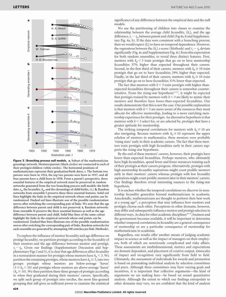
To explore the influence of mentor fecundity and age difference onprotege fecundity, we partition proteges according to the fecundity oftheir mentors and the age difference between mentor and protege,tc 2 tp. Given our findings (Supplementary Discussion and Sup-plementary Figs 2 and 3), it is clear that age differences affect fecundityin a nonrandom manner for proteges whose mentors have kp , 3. Wepartition the remaining proteges, whose mentors have kp $ 3, into twogroups: proteges whose mentors are below-average ‘haves’(3 # kp , 10) and proteges whose mentors are above-average ‘haves’(kp $ 10). We then partition these three groups of proteges accordingto when they graduated during their mentors’ careers. Specifically,we split each group of proteges into terciles, the most fine-grainedgrouping that still gives us sufficient power to examine the statistical
significance of any differences between the empirical data and the nullmodels.
We use the partitioning of children into classes to examine therelationship between the average child fecundity, Ækcæ, and the agedifference, tc 2 tp, between parent and child (Fig 4a, b and Supplemen-tary Fig. 4a, b). If the data were consistent with a branching process,then we would expect Ækcæ to have no temporal dependence. However,the regressions between the Ækcæ z-score (Methods) and tc 2 tp deviatesignificantly (Fig. 4c and Supplementary Fig. 4c) from this expectationfor both random ensembles, to reveal three distinct features. First,mentors with kp , 3 train proteges that go on to have mentorshipfecundities 37% higher than expected throughout their careers.Second, in the first third of their careers, mentors with kp $ 10 trainproteges that go on to have fecundities 29% higher than expected.Finally, in the last third of their careers, mentors with kp $ 10 trainproteges that go on to have fecundities 31% lower than expected.
The fact that mentors with k , 3 train proteges with higher-than-expected fecundities throughout their careers is somewhat counter-intuitive. From the rising-star hypothesis11,12, it might be expectedthat proteges trained by mentors with k , 3 are likely to mimic theirmentors and therefore have lower-than-expected fecundities. Ourresults demonstrate that this is not the case. One possible explanationis that mentors with k , 3 are more aware of the resources they mustallocate for effective mentorship, leading to a more enriching men-torship experience for their proteges. An alternative hypothesis is thatmentors with k , 3 select for, or are selected by, proteges that have agreater aptitude for mentorship.
The striking temporal correlations for mentors with kp $ 10 arealso intriguing. Because mentors with kp $ 10 represent the upperechelon of mentors in mathematics, these mentors were probably‘rising stars’ early in their academic careers. The fact that these men-tors train proteges with high fecundities early in their careers sup-ports the rising-star hypothesis.
By the end of these mentors’ careers, however, their proteges havelower-than-expected fecundities. Perhaps mentors, who ultimatelyhave high fecundities, spend fewer and fewer resources training eachof their proteges as their careers progress. Alternatively, proteges withhigh mentorship fecundity aspirations might court prolific mentorsearly in their mentors’ careers whereas proteges with low fecundityaspirations might court prolific mentors later in their mentors’ careers.Our findings therefore reveal interesting nuances to the rising-starhypothesis.
It is unclear whether the temporal correlations we discover in men-torship fecundity generalize beyond mathematicians in academia.Anecdotally, mathematicians are thought to perform their best workat a young age27, a perception that may influence how mentors andproteges choose each other. Perceptions in other domains, however,may differ and subsequently influence mentor and protege selection indifferent ways. As data for other academic disciplines18,19, business andthe government becomes available, it will be important to determinewhether temporal correlations in fecundity are a general consequenceof mentorship or are a particular consequence of mentorship formathematicians in academia.
Regardless, our results offer another means of judging academicimpact in science as well as the impact of managers on their employ-ees, both of which are notoriously complicated and risky affairs.These assessments are multidimensional, metrics and expectationsare domain dependent, and placement of creative output, timescalesof impact and recognition vary significantly from field to field.Ultimately, the assessment of individuals for awards and promotionis based on painstaking individual analysis by selection committeesand peers. Although these committees may have varying goals andincentives, it is important that collective arguments—the kind ofarguments we are making here—be based on sound quantitativeanalysis. Although the extent to which our findings extrapolate toother domains may vary, we are confident that the kind of analysis
H. D. Kloosterman
W. Tollmien
B. A. Griffith
K. A. Hirsch
1920 1930 1940 1950 1960 1970
Graduation year, t
a
b
c
Em
piri
cal n
etw
ork
Gen
erat
ing
ense
mb
le I
Gen
erat
ing
ense
mb
le II
Figure 3 | Branching process null models. a, Subset of the mathematiciangenealogy network. Mentors/parents (black circles) are connected to each oftheir proteges/children (white circles). The horizontal positions ofmathematicians represent their graduation/birth dates, t. The bottom twoparents were born in 1924, the top two parents were born in 1937, and allfour parents have a child born in 1958. From a parent’s perspective, threeessential features of the empirical network must be preserved in randomnetworks generated from the two branching process null models: the birthdate, tp, the fecundity, kp, and the chronology of child births, {tc}. b, Randomnetworks from ensemble I preserve these three essential features. Solid redlines highlight the links in the empirical network whose end points can berandomized. Dashed red lines illustrate one of the possible randomizationmoves after switching the corresponding pair of links. We note that the agedifference between parent and child is not preserved. c, Random networksfrom ensemble II preserve the three essential features as well as the agedifference between parent and child. Solid blue lines of the same colourhighlight the links in the empirical network whose end points can berandomized. Dashed blue lines illustrate one of the possible randomizationmoves after switching the corresponding pair of links. Random networks foreach ensemble are generated by attempting 100 switches per link (Methods).
LETTERS NATURE | Vol 465 | 3 June 2010
624Macmillan Publishers Limited. All rights reserved©2010

presented here will serve to elevate the discourse on scientific andmanagerial impact.
METHODS SUMMARYData acquisition. We use data from the Mathematics Genealogy Project17 to
identify the 7,259 protege mathematicians that are in the giant component28 and
graduated between 1900 and 1960, of which 4,447 have linked publication
records through the American Mathematical Society’s research database
MathSciNet. We use a text-matching algorithm29 to semi-automatically match
members of the NAS with mathematicians from the Mathematics Genealogy
Project.
Monte Carlo hypothesis testing for p(kjt). We use Monte Carlo hypothesis
testing30 to determine whether equation (1) with maximum-likelihood23 para-
meters H can be rejected as a candidate model for p(kjt) at the a 5 0.05 signifi-
cance level.
Random-network generation. We use a variation of the Markov chain Monte
Carlo algorithm25,26 to construct each of the 1,000 random networks in ensembles
I and II. Specifically, we restrict the switching of end points of links p R c that
belong to the same link class L, where the link classes are defined as
LI(t) 5 {p R cjtc 5 t} and LII(s, t) 5 {p R cjtp 5 s, tc 5 t} for networks from
ensembles I and II, respectively. Each link class can be thought of as a subgraph,
which can then be randomized in the usual way by attempting 100 switches per
link in the class25,26.
Average-fecundity z-score. By the central limit theorem, the average of variates
drawn from p(kcjtc) is normally distributed because p(kcjtc) is well described by a
mixture of discrete exponential distributions that has finite variance. Given a set
of child fecundities, Kc 5 {kc}, we quantify how significantly a subset of these
child fecundities, Kc*, Kc, deviates from Kc by measuring the z-score of Ækcæ, the
average child fecundity of all nodes within the subset Kc*, compared with Ækcæs,
the average child fecundity computed for children within a subset equivalent to
Kc* in the synthetic networks. That is, we compute z 5 (Ækcæ 2 m)/s, where m is
the ensemble average of {Ækcæs} and s is the standard deviation of the ensemble
{Ækcæs} over the 1,000 realizations generated for our null models.
Full Methods and any associated references are available in the online version ofthe paper at www.nature.com/nature.
Received 21 December 2009; accepted 19 March 2010.
1. Kram, K. E. Mentoring at Work: Developmental Relationships in Organizational Life(Scott Foresman, 1985).
2. Chao, G. T., Walz, P. M. & Gardner, P. D. Formal and informal mentorships: acomparison on mentoring functions and contrast with nonmentoredcounterparts. Person. Psychol. 45, 619–635 (1992).
3. Scandura, T. A. Mentorship and career mobility: an empirical investigation. J.Organ. Behav. 13, 169–174 (1992).
4. Aryee, S., Chay, Y. W. & Chew, J. The motivation to mentor among managerialemployees. Group Organ. Manage. 21, 261–277 (1996).
–0.1 0.0 0.1–3
–2
–1
0
1
2
3
Inte
rcep
t
–0.1 0.0 0.1Slope
–0.1 0.0 0.1100
101
102
10–2
10–1
100
10–3P
robab
ility density
Cum
ulat
ive
dis
trib
utio
n
Child fecundity, kc
kp < 3 3 ≤ kp < 10 kp ≥ 10
⟨kc⟩
z-s
core
Ens. IEarlyMiddleLate
10
10 20 30 400 10 20 30 400 10 20 30 400
20 30 40
–4
–2
0
2
4
10 20 30 40Age difference, tc – tp (yr)
10 20 30 40
1900s1910s1920s1930s1940s1950s
P = 0.009 P = 0.366
c
P < 0.001
= 2.2= 2.6
⟨kE⟩⟨kM⟩⟨kL⟩
⟨kE⟩⟨kM⟩⟨kL⟩
⟨kE⟩⟨kM⟩⟨kL⟩ = 1.2
= 1.7= 0.8= 1.3
a
= 2.5= 0.8= 0.3
Slope, 0.023Intercept, 0.18
Slope, 0.026Intercept, –0.42
b
Slope, –0.10Intercept, 2.1
Figure 4 | Effect of age difference between mentor and protege, tc 2 tp, onprotege fecundity. a, Fecundity distribution of children born during the1910s (for which the average fecundity was 1.4) to parents with kp , 3,3 # kp , 10 and kp $ 10, compared with the expectation from ensemble I(grey line). We separate children into terciles (early, middle, late) accordingto tc 2 tp, and denote the average fecundities of the children born early,middle and late in their parents’ lives as ÆkEæ, ÆkMæ and ÆkLæ, respectively. Theaverage fecundity of children born to parents with kp , 3 is higher thanexpected, regardless of whether they were born during the early, middle orlater part of their parents’ lives. We also note that the average fecundity ofchildren born to parents with kp $ 10 decreases throughout their parents’lives. b, We quantify the significance of these trends during each decade(coloured symbols) by computing the z-score of the average child fecundity,Ækcæ, compared with the average child fecundity in networks from ensemble I.This information is summarized by identifying the linear regression (solid
black line; slope and intercept as shown). The regression lines for networksfrom our null model (grey lines) vary around the expectation of our nullmodel (dashed black line). c, Significance of linear regressions in b. Wecompare the slope and intercept of the empirical regression (black circle)with the distribution of the slope and intercept of the same quantitiescomputed from the null model. Because these quantities are approximatelydistributed as a multivariate Gaussian, we compute the equivalent of a two-tailed P value by finding the fraction of synthetically generatedslope–intercept pairs that lie outside the equiprobability surface of themultivariate Gaussian (dashed ellipse). The slopes and intercepts of theregressions for children of parents with low (P 5 0.009) and high (P , 0.001)fecundities are significantly different from the expectations for the nullmodel, consistent with the data displayed in a. Comparisons withexpectations from random networks from ensemble II yield the sameconclusions (Supplementary Fig. 4).
NATURE | Vol 465 | 3 June 2010 LETTERS
625Macmillan Publishers Limited. All rights reserved©2010

5. Allen, T. D., Poteet, M. L., Russell, J. E. A. & Dobbins, G. H. A field study of factorsrelated to supervisors’ willingness to mentor others. J. Vocat. Behav. 50, 1–22 (1997).
6. Donaldson, S. I., Ensher, E. A. & Grant-Vallone, E. J. Longitudinal examination ofmentoring relationships on organizational commitment and citizenship behavior.J. Career Dev. 26, 233–249 (2000).
7. Payne, S. C. & Huffman, A. H. A longitudinal examination of the influence ofmentoring on organizational commitment and turnover. Acad. Manage. J. 48,158–168 (2005).
8. Kram, K. E. & Isabella, L. A. Mentoring alternatives: the role of peer relationships incancer development. Acad. Manage. J. 28, 110–132 (1985).
9. Higgins, M. C. & Kram, K. E. Reconceptualizing mentoring at work: adevelopmental network perspective. Acad. Manage. Rev. 26, 264–283 (2001).
10. Allen, T. D., Poteet, M. L. & Burroughs, S. M. The mentor’s perspective: aqualitative inquiry and future research agenda. J. Vocat. Behav. 51, 70–89 (1997).
11. Green, S. G. & Bauer, T. N. Supervisory mentoring by advisers: relationships withdoctoral student potential, productivity, and commitment. Person. Psychol. 48,537–562 (1995).
12. Singh, R., Ragins, B. R. & Tharenou, P. Who gets a mentor? A longitudinalassessment of the rising star hypothesis. J. Vocat. Behav. 74, 11–17 (2009).
13. Allen, T. D., Poteet, M. L. & Russell, J. E. A. Protege selection by mentors: whatmakes the difference? J. Organ. Behav. 21, 271–282 (2000).
14. Allen, T. D. Protege selection by mentors: contributing individual andorganizational factors. J. Vocat. Behav. 65, 469–483 (2004).
15. Ragins, B. R. & Scandura, T. A. Burden or blessing? Expected costs and benefits ofbeing a mentor. J. Organ. Behav. 20, 493–509 (1999).
16. Paglis, L. L., Green, S. G. & Bauer, T. N. Does adviser mentoring add value? Alongitudinal study of mentoring and doctoral student outcomes. Res. High. Ed. 47,451–476 (2006).
17. North Dakota State University. The Mathematics Genealogy Project Æhttp://genealogy.math.ndsu.nodak.eduæ (accessed, November 2007).
18. Bourne, P. E. & Fink, J. L. I am not a scientist, I am a number. PLoS Comput. Biol. 4,e1000247 (2008).
19. Enserink, M. Are you ready to become a number? Science 323, 1662–1664 (2009).20. King, J. A review of bibliometric and other science indicators and their role in
research evaluation. J. Inf. Sci. 13, 261–276 (1987).
21. Moed, H. F. Citation Analysis in Research Evaluation (Springer, 2005).22. Hirsch, J. E. An index to quantify an individual’s scientific research output. Proc.
Natl Acad. Sci. USA 102, 16569–16572 (2005).23. Bishop, C. M. Pattern Recognition and Machine Learning (Springer, 2007).24. Athreya, K. B. & Ney, P. E. Branching Processes (Courier Dover, 2004).25. Milo, R., Kashtan, N., Itzkovitz, S., Newman, M. E. J. & Alon, U. On the uniform
generation of random graphs with prescribed degree sequences. Preprint atÆhttp://arxiv.org/abs/cond-mat/0312028æ (2004).
26. Itzkovitz, S., Milo, R., Kashtan, N., Newman, M. E. J. & Alon, U. Reply to ‘‘Commenton ‘Subgraphs in random networks’’’. Phys. Rev. E 70, 058102 (2004).
27. Hardy, G. H. A Mathematician’s Apology (Cambridge Univ. Press, 1940).28. Stauffer, D. & Aharony, A. Introduction to Percolation Theory 2nd edn (Taylor &
Francis, 1992).29. Chapman, B. & Chang, J. Biopython: python tools for computational biology. ACM
SIGBIO Newslett. 20, 15–19 (2000).30. D’Agostino, R. B. & Stephens, M. A. Goodness-of-Fit Techniques (Dekker, 1986).
Supplementary Information is linked to the online version of the paper atwww.nature.com/nature.
Acknowledgements We thank R. Guimera, P. McMullen, A. Pah, M. Sales-Pardo,E. N. Sawardecker, D. B. Stouffer and M. J. Stringer for comments and suggestions.L.A.N.A. gratefully acknowledges the support of US National Science Foundationawards SBE 0830388 and IIS 0838564. All figures were generated usingPYGRACE (http://pygrace.sourceforge.net) with colour schemes fromColorBrewer 2.0 (http://colorbrewer.org).
Author Contributions R.D.M. analyzed data, designed the study and wrote thepaper. J.M.O. and L.A.N.A. designed the study and wrote the paper.
Author Information Reprints and permissions information is available atwww.nature.com/reprints. The authors declare no competing financial interests.Readers are welcome to comment on the online version of this article atwww.nature.com/nature. Correspondence and requests for materials should beaddressed to J.M.O. ([email protected]) or L.A.N.A.([email protected]).
LETTERS NATURE | Vol 465 | 3 June 2010
626Macmillan Publishers Limited. All rights reserved©2010
METHODSMathematics Genealogy Project data. We study a prototypical mentorship
network collected from the Mathematics Genealogy Project17, which aggregates
the graduation dates, mentors and advisees of 114,666 mathematicians from as
early as 1637. From this information, we construct a mathematician genealogy
network in which links are formed from a mentor to each of his or her k proteges.
The data collected by the Mathematics Genealogy Project are self-reported, so
there is no guarantee that the observed genealogy network is a complete descrip-
tion of the mentorship network. In fact, 16,147 mathematicians do not have a
recorded mentor and, of these, 8,336 do not have any recorded proteges. Toavoid having these mathematicians distort our analysis, we restrict our analysis
to the 90,211 mathematicians that comprise the giant component28 of the net-
work; that is, we restrict our analysis to the largest set of connected mathema-
ticians in the mathematician genealogy network.
Although the Mathematics Genealogy Project contains information on math-
ematicians from as early as 1637, this does not necessarily indicate that all of these
records are representative of the evolution of the network. For example, before
1900 the Project records fewer than 52 new graduates per year worldwide.
Furthermore, because mathematicians often have mentorship careers lasting
50 years or more, we are not guaranteed to have complete mentorship records
for mathematicians who graduated after 1960. We therefore restrict our analysis
to the 7,259 protege mathematicians who graduated between 1900 and 1960, for
whom we believe that the graduation and mentorship record is the most reliable.
MathSciNet data. Of the 7,259 protege mathematicians that graduated between
1900 and 1960, 4,447 of them have linked MathSciNet publication records,
which are used in our analysis.
US National Academy of Science data. The US National Academy of Science
maintains two databases of its membership. The first database consists of alldeceased members elected to the NAS from as early as 1863. This database
records the name of the inductee, their election year, their date of death and a
link to a biographical sketch. The second database consists of all active members
of the NAS. This database records the name of the inductee, their institution,
their academic field and their election year.
The challenge to matching this data with the Mathematics Genealogy Project
data is that there is no direct link between a member of the NAS and the
Mathematics Genealogy Project, and vice versa. This is further confounded by
the fact that some members of the NAS have the same name. To circumvent these
problems, we use a text-matching algorithm29 to semi-automatically detect whether
a member of the NAS matches a name in the Mathematics Genealogy Project
database. We use this procedure to curate the 269 members of the NAS that
definitively match mathematicians in the Mathematics Genealogy Project database.
Monte Carlo hypothesis testing for p(kjt). Given a model, M, with parameters
Ht for the empirically observed fecundity distribution, p(kjt), we use Monte
Carlo hypothesis testing to determine whether it can be rejected as a candidate
model for p(kjt) (ref. 30). The Monte Carlo hypothesis testing procedure is as
follows. First, we calculate the best-estimate parameters, ht, for model M at time t
using maximum-likelihood estimation23. Second, we compute the test statistic, S
(detailed below), between the model M(Ht) and the empirical fecundity distri-
bution, p(kjt). Next, we generate a synthetic fecundity distribution, ps(k), from
model M(Ht) using the best-estimate parameters, ht, and we treat the synthetic
data exactly the same as we treated the empirical data: first, we calculate the best-
estimate parameters, Hs, for model M from maximum-likelihood estimation;
second, we compute the test statistic, Ss, between the model M(Hs) and the
synthetic fecundity distribution, ps(k). We generate synthetic fecundity distribu-
tions and their corresponding synthetic test statistics until we accumulate an
ensemble of 1,000 Monte Carlo test statistics, {Ss}. Finally, we calculate a two-
tailed P value with a precision of 0.001. As is customary in hypothesis testing, we
reject the model M at time t if the P value is less than a threshold value. We select a
P-value threshold of 0.05; that is, if less than 5% of the synthetic data sets exhibit
deviations in the test statistic that are larger than those observed empirically, the
model is rejected at time t.
Because we are conducting hypothesis tests with the fecundity distribution
p(kjt), which is a distribution with a discrete support, it is important to use a test
statistic S that is appropriate for testing discrete distributions. We use the x2 test
statistic whereby we bin p(kjt) such that each bin has at least one expected
observation according to the model M(Ht). This binning prevents observations
that are exceptionally rare from dominating our statistical test and skewing our
results.
Random-network generation. We use the Markov chain Monte Carlo algo-
rithm25,26 to build random networks from the mathematician genealogy net-
work. The standard version of this algorithm inherently preserves the
fecundity of each individual, but it does not preserve the chronology of child
births, {tc}, for each parent. To obtain random networks belonging to ensemble I
or ensemble II, we restrict the switching of end points of links p that belong to the
same link class L, where the link classes are defined as LI(t) 5 {p R cjtc 5 t} and
LII(s, t) 5 {p R cjtp 5 s, tc 5 t} for networks from ensembles I and II, respectively.
Each link class can be thought of as a subgraph, which can then be randomized
using the Markov chain Monte Carlo algorithm. Here, we attempt 100 switches
per link in each link class, which sufficiently alters random networks away from
the original empirical network25,26. We repeat this procedure 1,000 times to
generate a set of 1,000 random networks for each ensemble.
Average-fecundity z-score. The average of variates drawn from p(kcjtc) is normally
distributed because p(kcjtc) is well described by a mixture of discrete exponential
distributions—a distribution with finite variance—and, thus, the central limit
theorem applies. Given a set of child fecundities, Kc 5 {kc}, we quantify how
significantly a subset, Kc*, of these child fecundities deviates from Kc, by measuring
the z-score of Ækcæ, the average child fecundity of all nodes within the subset Kc*,
compared with Ækcæs, the average child fecundity computed for children within a
subset equivalent to Kc* in the synthetic networks. That is, we compute
z 5 (Ækcæ 2 m)/s, where m is the ensemble average of {Ækcæs} and s is the standard
deviation of the ensemble {Ækcæs} over the 1,000 realizations generated for our null
models.
doi:10.1038/nature09040
Macmillan Publishers Limited. All rights reserved©2010