Embed Size (px)
Citation preview
The Stochastic Recovery Rate in CDS: Empirical
Test and Model
Chanatip Kitwiwattanachai
University of Connecticut
November 25, 2012
Abstract
Recovery rates have been treated as a constant in the literature. However, recent empirical
findings suggest that realized recovery rates are stochastic and highly dependent on the industry
condition. It is hard to separate the effect of risk-neutral probability of default and risk-neutral
recovery rates in CDS. This paper uses the unique characteristic of ex post (physical) recovery
rates to capture the ex ante (risk-neutral) recovery rates in CDS spreads. I document that CDS
spreads incorporate the information of expected recovery rates. I derive a first-passage-time
structural model for stochastic recovery rates linked to industry conditions. This model can
be used to extract implied recovery rates from CDS spreads. If the industry is in distress, the
expected risk-neutral recovery rate will be lower by 20%.
This paper is based, in part, on my dissertation completed at the University of Illinois, Urbana-Champaign.
I am indebted to my adviser, Neil Pearson, and my dissertation committee, George Pennacchi, Tim Johnson and
Heitor Almeida for their assistance. I am also grateful to Prachi Deuskar, Jay Wang, Slava Fos, Charles Kahn,
Mathius Kronlund and seminar participants at the Uniersity of Illinois, Urbana-Champaign. Remaining errors are my
responsibility
0
Introduction
Credit derivatives provide insurance against the risk of a default on bonds. The price of credit
derivatives depends on two main factors: the risk-neutral probability of default and the risk-neutral
recovery rates. Research on credit derivatives focuses mostly on the first factor, while regarding the
second factor as a constant at about 0.4 to 0.5 of the face value. However, recent research has found
that realized recovery rates are not constant, ranging from 0.2 to 0.7. Moreover, they correlate highly
with the probability of default, i.e., recovery rates are low when default rates are high, and vice versa.
Recovery rates are hard to model and estimate. Defaults are rare and thus recoveries are also
rare. As a consequence, we lack understandings for both default probabilities and recovery rates.
Models for defaults have been developed and enable researchers to use CDS prices to back out
implied default probabilities instead of using the historical default data. CDS spreads are also more
informative about default than bond prices, since the bond market is much more complicated and less
liquid than the credit market (Longstaff et al. (2005)). This paper develops a model for stochastic
recovery rates and embed it in the CDS pricing model. With such a model, researchers can learn
about expected recovery rates from CDS data, similar to how default probabilitites can be extracted
from CDS.
Central to corporate finance is the question of captial structure. Central to capital structure
theory is the cost of default or recovery rates. Reseachers attempt to estimate this parameter (for
example, Davydenko, Strebulaev and Zhao (2012)) but the data are rare and the desired quantity
should be risk-adjusted for the purpose of capital structure theory (Almeida and Philippon (2007)).
The implied recovery rates from CDS spreads are available in abundance and have already been
risk-adjusted by the market.
In this paper I seek to understand and parametrize the risk-neutral recovery rates in CDS. To
model recovery rates as stochastic, it is crucial to know which factors drive expected recovery rates.
The three main papers on realized recovery rates are Altman et al. (2005), Shleifer and Vishny
(1992), and Acharya et al. (2007). The main conclusion is that recovery rates depend on industry
1

characteristics (asset redeployability) and industry distress (asset specificity). Recovery rates are
higher when assets are redeployable, which in turns depend on the industry the firms are in. Recovery
rates are lower if the firms default when the industry is in distress and the assets must be sold to
industry outsiders who face significant costs of managing assets. These two factors are the main
driver of my model, especially the industry distress factor which makes the recovery rates stochastic.
Before the model, I need to show that CDS prices actually incorporate this information.
Empirically, for CDS, it has been difficult to separate the effect of risk-neutral recovery rates from
the risk-neutral probability of default. The main difficulty is that both factors, which are stochastic
with high correlations, are multiplied together to form a price. I establish the fact that recovery
rates are priced into the credit derivatives ex ante, in addition to the effect of the probability of
default. The key to distinguish the effect of recovery rates from the probability of default is industry
characteristics and industry distress factors. Using these two factors, and controlling for other factors
that affect the CDS spreads, including the probability of default, I can detect the recovery factor
in credit derivative prices. I conduct a battery of tests to verify that these factors do represent the
recovery rates and not default probabilities. This finding assures that CDS spreads have information
about expected recovery rates. I then proceed to the model of stochastic recovery rates.
I incorporate the stochastic recovery rates into the credit risk model. I use the first-passage-time
structural model to calculate the probability of default. I parametrize the recovery rate so that it
depends on industry characteristics and industry distress as suggested by the data. This step links
the unobserved ex ante (risk-neutral) recovery rates to observable parameters such as industry index.
I then calibrate the model to the data to find the value of parameters for risk-neutral recovery rates.
The result is that the risk-neutral recovery rate will be lower by 20% if the industry is in distress
during the firm’s default. This step shows that the model is valid with reasonable magnitude for
implied stochastic recovery rates. With this model, researchers can find implied recovery rates and
default probabilities from CDS data. A more sophisticated estimation method may be required and
this can be a subject of future research.
Few papers explore the implied (risk-neutral) recovery rates in fixed income products. The closest
2
ones are Bakshi et al. (2006), Le (2007) and Pan and Singleton (2008). The key difference for my
paper is that I use the unique characteristics of recovery rates, namely the link to industry conditions,
in my model while other papers treat recovery rates more from a technical standpoint. Also, my
paper is based on a structural model which incorporates more economic intuition while other papers
are based on a reduced-form model.
The paper proceeds as follows. Section 1 describes the CDS pricing model. Section 2 describes how
to calculate the probability of default. Section 3 describes the CDS data. Section 4 is an empirical
analysis of the implied recovery factor in CDS. Section 5 is a robustness check. Section 6 describes
the theoretical model I derive to capture the empirical findings. I then conclude in the final section.
1 CDS Pricing Model
In this section I introduce the CDS pricing model that will incorporate all the factors needed to
be considered in the empirical analysis. A Credit Default Swap (CDS) is a contract that provides
insurance against the risk of a default by a particular company. The company is known as the
reference entity and a default by the company is known as a credit event. The buyer of this contract
obtains the right to sell bonds issued by the reference entity for their face value when a credit event
occurs. On the other hand, the CDS seller agrees to buy the bonds for their face value when a credit
event occurs, thus bearing the risk of default.
The CDS buyer makes periodic payments to the seller until the end of the life of the CDS or until
a credit event occurs. The settlement, in the event of a default, involves either physical delivery of
the bonds or a cash payment. The observable quantity in the market is the payment by the CDS
buyer, also known as CDS spreads. The CDS spreads in a liquid market reflect the fair price for
default insurance, i.e., the spreads must make the expected value of the buyer’s periodic payments
equal to the expected value of the seller’s losses in case of default.
In a no-arbitrage model, the CDS spreads should make the present value of payments from the
buyer (fixed leg) equal to the present value of losses by the seller (contingent leg). Let S be the CDS
3
spread and R the risk-neutral expected recovery rate if default occurs. Let Q(t) be the risk-neutral
cumulative probability of default up to time t, thus the risk-neutral probability of survival up to
time t = 1−Q(t). Let d be the accrual days betIen payment dates, for example, if the payments are
made quarterly, then d = 0.25. Let D(t) be the discount factor. Then
PV [fixed leg] =N∑i=1
D(ti)(1−Q(ti))Sdi
PV [contingent leg] = (1−R)N∑i=1
D(ti)(Q(ti)−Q(ti−1))
The first equation represents the expected payment from the buyer, by multiplying payments with
the probability of survival. The second equation represents the expected payment from the seller, by
multiplying the payment in case of default with the default probability. By equating the two present
values, I can represent S as:
S =
(1−R)N∑i=1
D(ti)(Q(ti)−Q(ti−1))
N∑i=1
D(ti)(1−Q(ti))di
(1)
The above equation is for discrete time. The continuous-time model uses the same intuition. I take
CDS spread formula, given for the contract starting from time 0 to T , from Hull, Predescu and White
(2009):
S =
(1− R̂)(1 + a∗)T∫0
q(u)v(u)du
T∫0
q(u)[h(u) + e(u)]du+ (1−T∫0
q(u)du)h(T ))
(2)
where
T : The period of the contract
q(u) : Probability density function (pdf) of default at time u in a risk-neutral world
R̂ : Expected recovery rate on the reference obligation in a risk-neutral world
h(u) : Present value of payments at the rate $1 per year on payment dates betIen time zero and
time u
e(u) : Present value of accrual payment at time u equal to u − u∗ where u∗ is the payment date
4
immediately preceding time u
v(u) : Present value of $1 received at time u
a∗ : Average value of accrued interest rate on the reference obligation for the period 0 to T
I will use the discrete-time model to guide my empirical analysis, but I will use the continuous-
time model when I modify the recovery rate function in the theoretical section. From Eq(1), the
factors that affect CDS spreads are the risk-neutral probability of default, the risk-neutral recovery
rate, and the interest rate (discount factor). In this paper I assume the interest rate is constant when
investors price the financial instruments. I can then write D(t) = e−rt.
2 The Probability of Default
There are two main approaches to model the probability of default: structural models and reduced-
form models. A structural model characterizes defaults as asset values falling below default barriers.
A reduced-form model abstracts away from the fundamentals of the firms and characterizes defaults
as a Poisson process. The advantage of a structural model is that it is economically intuitive, while
the advantage of a reduced-form model is that it is easier to fit the data to the ”unobserved” default
intensity. In this paper I only use a structural model approach. The choice here is not only because
of the economic intuition, but also because I will incorporate the results from corporate finance into
the recovery factor. In corporate finance models, assets and debts have ”physical” meaning, not just
a mathematical concept, and so I do not want to abstract away from the physical model. I would
like to have a unified view of default processes and recoveries in a single model.
In a structural model, firms default when they cannot fulfill financial obligations. In mathematical
terms, the firm defaults when its value falls below the debt barrier. The first generation model by
Merton calculates the probability of default at the date of debt maturity, for example 1 year from
now. The firm can only default at the date of debt maturity. The next generation of model, pioneered
by Black and Cox (1976), characterizes default as the first passage time of the firm value across the
5
debt barrier. In this model firms can default any time betIen now and the date of debt maturity.
Mathematically it is much harder to calculate the first passage time density as in the Black and
Cox model than to calculate the probability of default at maturity date as in the Merton model. In
empirical analysis section I use the probability of default from the Merton model, which was modified
by Bharath and Shumway (2008). I briefly describe the calculation method here.
In the risk-neutral measure, the (unobserved) value of a firm follows a geometric Brownian motion
dV = rV dt+ σV V dWQ (3)
which is a standard setup and r is the risk-free rate. The firm issues a discounted bond maturing at
time T. Under this assumption, the equity of the firm is a call option on the underlying value with a
strike price equal to the face value of the firm’s debt and a time-to-maturity of T . The value of equity
as a function of the unobserved total value of a firm can be described by the Black-Scholes-Merton
formula.
Specifically, Merton shows that the equity value of a firm satisfies
E = VN(d1)− e−rTFN(d2) (4)
where E is the market value of the firm’s equity, F is the face value of debt, N(.) is the cumulative
standard normal distribution function, d1 is calculated from
d1 =ln(V/F ) + (r + 1
2σ2V T )
σV√T
(5)
and d2 = d1 − σV√T
The Merton model links the unobserved total value of the firm to the observed equity value.
Moreover, with a closed-form expression, I can link the volatility of the firm to the valatility of the
equity. It follows from Ito’s lemma that
σE =
(V
E
)∂E
∂VσV
=
(V
E
)N(d1)σV (6)
6
where the second line comes from the fact that ∂E∂V
= N(d1) from the partial derivative of Eq(4).
From Eq(4) and Eq(6), I have two equations and two unknowns (V and σV ). Thus, I can solve
for the unobserved variables V and σV , given the value of E and σE.
Once I solve for V and σV , risk-neutral the distance to default (DD) can be calculated as
DD =ln(V/F ) + (r − 1
2σ2V )
σV√T
(7)
and then the risk-neutral probability of default (PD) is given by
PD = N(−DD) (8)
The probability of default here characterizes the probability that the firm value will fall below the
face value of debt at maturity.
While the mentioned method is straightforward, it involves solving simultaneous equations for
every observation. Bharath and Shumway (2008) explores an alternative way to calculate the prob-
ability of default. The method is based on the same economic intuition about the default process,
but does not require solving simultaneous equations. I briefly describe their method here:
To begin, they approximate the market value of each firm’s debt with the face value of its debt,
DBS = F (9)
Where BS stands for Bharath-Shumway. The volatility of the debt is correlated with the equity
volatility
σD,BS = 0.05 + 0.25 ∗ σE (10)
The 5 percent represents the term structure volatility and the 25 percent times equity volatility
represents the volatility associated with the default risk. Thus, the approximation of the total
volatility of the firm is calculated by
σV,BS =E
E +DBS
σE +DBS
E +DBS
σD,BS
=E
E + FσE +
F
E + F(0.05 + 0.25 ∗ σE) (11)
7

This approximation captures the same information that is captured by the Merton model, but without
having to solve simultaneous equations. The naive distance to default is then given by:
DDBS =ln((E + F )/F ) + (r − 1
2σ2V,BS)
σV,BS√T
(12)
The DDBS is easy to compute and also represents the same information as the Merton DD. Finally
the probability of default is given by
PDBS = N(−DDBS) (13)
In section 4.5 of Bharath and Shumway (2008), the authors regress the log of CDS spreads with the
log of PDBS and compare the result with the regression with the log of Merton PD. It should be
noted that they use 1-year PD while the CDS contract is 5-year. The reason is that 1-year PD is
highly correlated with 5-year PD, and the log specification of this regression makes the intercept
reflect the average level of the probability. The regression results show that both variables are
statistically significant, but the R2 of log(PDBS) is higher than log(Merton PD). Moreover, when
adding both PDBS and Merton PD in the same regression, the statistical significance of the Merton
PD is driven out by the PDBS. They conclude that the functional form of the probability of default
is more important than the solution procedure.
Due to the result of this paper and relative ease of computation, I will use the PDBS in my
empirical analysis instead of the original Merton PD. In the robustness check I use the Merton PD
and the result still holds.
3 Data
I use CDS data from Credit Market Analysis (CMA), acquired by CME on March 25, 2008. The
data are daily ranging from January 2004 to May 2008. For this paper I use only 5-year CDS data
because they are the most common and most liquid. From daily data, I change the interval to
monthly, because it is known that the CDS spreads have high autocorrelations, possibly because of
illiquidity. I use the spreads at the end of month as monthly data. I match firms in my CDS dataset
8
with CRSP database using Ticker symbols. The summary statistics of the CDS data are presented
in Table 1.
To detect the effect of recovery rates, I use industry dummy variables and industry distress indi-
cators. The industry dummy variables are assigned according to the firm’s Siccode. I divide firms
into 10 industries based on the Siccodes on Kenneth French’s website. The percentage of firms in
each industry in my dataset is shown in Table 2.
The industry distress indicators need to signify the state of the industry. According to Acharya et
al. (2007), there are various ways to define industry distress. The first is that the median stock return
for the industry of the defaulting firm falls below -30% annually. This accounts for 9% of the sample
data. The second is that one-year or two-year median sales growth for the industry is negative. The
third is that the average credit rating of other firms in the industry is below investment grade. The
three proxies give similar results in their paper and the first proxy is used for all subsequent analyses.
Following the first proxy of industry distress, I use the 10th percentile as a cutoff for distress. If
the industry return for that month is less than the 10th percentile, then industry distress indicator
is 1, otherwise it is 0. I use the 10th percentile cutoff here to be consistent with the literature; about
9-10% of the sample will be in distress. The result is also robust to other cutoff levels. The cutoff
comes from the historical data of industry returns for each industry during the 10-year period of
1994-2003. The distress cutoff for each industry is shown in Table 3.
To control for the probability of default, I calculate the probability of default using PDBS as
described in the last section. I use the equity data from CRSP and the debt data from Compustat.
Following Bharath and Shumway (2008), the face value of debt (F ) is calculated as (short-term debt
+ 0.5*long-term debt). The equity volatility (σE) is also calculated from monthly returns from CRSP,
and then adjusted to annual scale. I use the risk-free rate r = 2.5% for the drift in the risk-neutral
measure. I want to fix the interest rate effect in the probability of default. This assumption may be
relaxed and the main result still goes through.
Another important proxy for the probability of default is the firm’s ratings. In theoretical models,
9

PD should be sufficient statistics that capture all the information of default probabilities. However,
in the data, ratings are significant in explaining credit spreads even after controlling for PD (Aunon-
Nerin et al. (2002)). Even though ratings reflect physical instead of risk-neutral probability of
default, the two must be highly correlated, and I can use one as a proxy for another in the regression
analysis. Thus, in the regression I include the probability of default as reflected by the firm’s ratings.
I use S&P ratings available on Compustat. I then convert ratings into the equivalent probability of
default using Moody’s corporate idealized 5-year cumulative probability of default rates.
Other factors that may affect CDS spreads include interest rates as a discount factor. I use
Treasury bill rates of maturity 3-month and 5-year as a control. These are the shortest and longest
maturity interest rates that may affect CDS spreads. Investors may use different interest rates to
discount cash flows, but they should be in the range of these short and long term rates or their linear
combination. In the empirical analysis, I only include these two rates. The data are also from CRSP.
4 Empirical Results
The main hypothesis to test here is whether recovery rates are incorporated into the CDS spreads,
ex ante. The results from Acharya et al. (2007) indicate that industry characteristics and industry
distress determine physical recovery rates, ex post, in addition to the risk-neutral probability of
default. I will then look for the significance of industry dummy variables and industry distress
indicators in the regression with CDS data. The result is shown in Table 4.
The first column shows the full regression while the second column shows the regression without
the industry condition (only the probability of default and interest rates). The R2 in the second
column decreases from the first column by about 0.034 or 3.4%. The industry condition can explain
about 3.4% of the CDS spreads. Most of the variations in CDS spreads indeed come from the
probability of default. However, the industry condition is also highly significant and the economic
magnitude is big, especially for Distress. I now focus on the significance of the coefficients in the
first column.
10
After controlling for the probability of default and interest rates, the industry dummy variables
and industry distress indicators are still statistically significant. The variables I1− I9 are industry
dummy variables, where I1 = 1 if the firm is in industry number 1 and 0 otherwise, and similarly for
I2 to I9. Note that I cannot include I10 in the regression, otherwise I will get a linearly dependent
vector of I10 with I1 to I9. The industry effect of I10 is absorbed into the intercept in the regression.
All the industry dummy variables are significant. This indicates that the industry-specific asset is an
important factor to determine the expected recovery rates in CDS spreads. However, in this paper I
put more focus on the Distress factor, which is time-varying. The industry dummy can be regarded
as a constant which can vary by industry but will not explain the time-varying patterns of recovery
rates over time.
The variables Distress and lag(Distress) stand for the industry distress indicator and its 1-month
lag. Both variables are significant and the sign is positive as expected. If the industry is in distress,
then the recovery rates will be lower because it is hard to sell assets to non-defaulted firms in the
same industry. Thus, fire-sales effect, which will occur when the industry is in distress, is also priced
into the CDS spreads. The lag of Distress is included in the regression because I doubt that the CDS
market may not be liquid and thus the information of Distress may take time to be incorporated
into the price. Indeed, the lag of Distress is also significant in the regression. I will discuss more
about illiquidity effect in the robustness check section.
The magnitude of Distress is 0.4, which is very big in a log scale. This translates to about e0.4
- 1 = 0.5 or 50% decline in expected risk-neutral recovery rates if the industry is in distress. This
extreme magnitude can have many interpretations. First, it can mean that investors are very risk-
averse about recovery rates and thus a sharp decline in expected recoveries in distress. Second, it
can mean that my Distress condition is too extreme and thus the resulting magnitude is too high.
Third, it can mean that Distress is a proxy for some other factors as well, for example illiquidity
and time-varying risk premium. The third explanation is the most plausible and I provide evidence
in the robustness check section.
Probability of Default (PD) and Interest Rates are included as control variables in the regression.
11

With control variables, I make sure that industry characteristics and industry distress variables are
significant because of recovery rates, not the probability of default or other factors. Note that PD
and interest rates are also significant in the regression as I expect from the theoretical formula.
However, I focus only on the recovery rates and do not go into details about these two factors in this
paper.
Since this is a panel regression, I should also control for the firm fixed effect and time fixed effect.
I do the same regression with firm and time fixed effects and the result is shown in Table 5.
The first column is the same as the first column in the previous table. In the second column I add
firm fixed effect and yearly time fixed effect. In the third column I add firm fixed effect and monthly
time fixed effect.
From the second column, some of the industry characteristics (I1−I9) lose statistical significance.
This result is as expected. When I control for finer information (firm-level), then the cruder infor-
mation (industry-level) is no longer significant. The coefficients for Distress and lag(Distress) are
still significant although the magnitude is slightly smaller than the first column. Note that the R2
jumps by almost 20% when I include firm and time fixed effect.
In the third column, I see the same result for industry characteristics (I1−I9). However, Distress
and lag(Distress) have much lower magnitude than before, although they are still highly significant.
When I control for time fixed effect at the monthly level, then this information is highly correlated
with Distress. Industry conditions are highly correlated with the economy and month fixed effect
may be a proxy for the state of the economy for a given month. Nevertheless, after controlling for
month fixed effect, Distress is still highly significant. This means that the industry condition does
affect the recovery rates and this factor is not purely driven by the macro economy.
12

5 Robustness Check
The results from the last section indicate that industry characteristics and industry distress are
significant in determining CDS spreads. In other words, the recovery factor is priced into CDS spreads
ex ante. In this section, I check for the robustness of the result. In particular, I check whether other
factors may affect CDS spreads and make industry characteristics and industry distress no more
statistically significant in the empirical analysis.
The first factor is the state of the economy. Obviously the state of the economy will affect the
probability of default, recovery rates and interest rates and thus the CDS spreads. It can also affect
the level of risk-aversion of investors and change the probability in the risk-neutral measure. I control
for the state of the economy by using the S&P500 index returns from CRSP.
The second factor is the state of the industry. Acharya et al. (2007) indicates that the continuous
industry returns have no effect on recovery rates ex post; only the industry distress does. However,
ex ante, industry returns may affect the expected recovery rates. Moreover, the industry returns
may affect the probability of default. Thus, the industry returns can affect the CDS spreads and I
include them as a control variable. I use industry returns data from Kenneth French’s website.
The third factor is illiquidity. In a liquid market, the CDS spreads should reflect a fair price.
However, in an illiquid market, it can be the case that CDS spreads are higher because no one is
willing to provide credit protection. Illiquidity usually happens during the distressed period. Also,
different industries may have different liquidity for CDS protection. Thus, my results in the previous
section may reflect market illiquidity factor, not the recovery factor in CDS spreads. For robustness
check, I control for the illiquidity factor by using bid-ask spreads as is prevalent in the literature.
In theory I should include fixed effects in all regressions. However, from Table 5, including firm
fixed effect will naturally dry out the industry characteristics effect. Also, including month fixed
effect will naturally dry out the industry distress effect. Thus, in this section, I first run a regression
without fixed effects in one table and then run a regression with fixed effects in the next table.
13

Table 6 shows the result of the regression with control variables but without fixed effects. The
first column shows the original regression as in Table 4. The second column shows the regression
with additional S&P500 index returns as a control for the state of the economy. The third column
shows the regression with additional industry returns as a control for the state of the industry. The
fourth column shows the regression with log(Bid−Askspreads) as a control for illiquidity. The fifth
column shows the regression with all the control variables.
When I add index returns as a control in the second column, all the regression coefficients are the
same except for Distress, whose coefficient decreases from 0.40 to 0.31 but is still significant. The
coefficient for index returns itself is also highly significant with a negative sign as expected. This
means that the state of the economy can influence the CDS spreads in addition to the factors in the
original regression. More interestingly, the state of the economy can affect the recovery factor that
used to be captured by the industry distress factor. However, since Distress is still significant, I
see that industry distress still determines the recovery rates after controlling for the economy. The
lag(Distress) factor remains highly significant with high magnitude. Perhaps lag(Distress) is even
a better proxy for industry distress, because the CDS market may take some time to incorporate
this information into the price.
When I add industry returns as a control in the third column, all the regression coefficients are the
same except for Distress, whose coefficient decreases from 0.40 to 0.28 but is still highly significant.
The coefficient for industry returns itself is also highly significant with a negative sign as expected.
Similar to index returns, industry returns can affect the recovery factor that used to be captured
by the industry distress factor, even more so than index returns. However, since Distress is still
significant, the industry distress factor still determines the recovery rates after controlling for the
state of the industry.
When I add illiquidity as a control in the fourth column, most of the previous coefficients including
the I1 − I9 industry characteristics variables remain significant except for I2. The coefficients also
change from the original regression. The coefficient for illiquidity itself is highly significant with a
positive sign as expected. Thus, illiquidity does affect the CDS spreads that used to be captured by
14
the industry characteristics. The more drastic effect is on the Distress and lag(Distress) factors.
After controlling for illiquidity, the coefficients for Distress and lag(Distress) decrease from 0.40
to 0.20 and 0.39 to 0.19, respectively. This means that during the period of illiquid market, CDS
spreads are higher because it is hard to find a seller. Moreover, the market is usually illiquid when
the industry is also in distress, which is also when the recovery rates are expected to be lower. The
effect of recovery rates in distress, and also the effect of illiquidity on CDS spreads, were captured by
the Distress and lag(Distress) factors in the original regression. However, when I include illiquidity
factor as a control variable in this regression, I separate the effects of industry distress and illiquidity.
As a result, the coefficients for Distress and lag(Distress) decrease significantly. However, since
both factors are still highly significant, the industry distress factor still determines the recovery rates
after controlling for illiquidity.
Finally I include all control variables in the fifth column. The coefficients of I1-I9 are very similar
to the fourth column. The coefficient for lag(Distress) stays the same as in the fourth column, but
the coefficient for Distress decreases from 0.20 to 0.13 and becomes insignificant at 10% level. This
means that the illiquidity factor affects CDS spreads in a similar way as industry characteristics
and industry distress, more so than index returns and industry returns. The coefficient of Distress
decreases from the fourth column because Distress is also affected by index returns and industry
returns, as shown in the second and third column.
The magnitude of Distress and lag(Distress) in the last column is more realistic. The magnitude
of 0.13 and 0.19 in the log scale translates to e0.13 − 1 = 0.14 and e0.19 − 1 = 0.21, or 14% and 21%
decrease in risk-neutral recovery rates. This magnitude is also consistent with the result from my
theoretical section. Interestingly, Distress itself is not significant but lag(Distress) is still significant.
This can mean that the information about industry distress takes some time to be realized in the
market price because the CDS market is not perfectly liquid.
In sum, after controlling for all other factors that may affect CDS spreads, the industry charac-
teristics and industry distress factors are still highly significant. In particular, the significance of the
industry distress indicator confirms that the stochastic recovery rates are priced into CDS spreads,
15
ex ante.
Now I add in the firm and time fixed effects in the regression. The result is reported in Table 7.
The first column of Table 7 shows the regression with no fixed effect, the same as in the last
column of Table 6. The second column shows the regression with only firm fixed effect. The third
and fourth columns show the regression with firm-year and firm-month fixed effect. Note a jump in
R2 from the first column to the next three columns. Fixed effects indeed play a significant role in
explaining CDS spreads. Interestingly, the R2 is almost 90%. As complicated as CDS cash flows are,
only a handful of factors can explain almost 90% of all the spreads.
In the second column, after controlling for firm fixed effect, some of the industry characteristics
lose statistical significance. However, lag(Distress) is still highly significant with roughly the same
magnitude while Distress becomes significant at 10% level. The result in the third column is similar
to the second column. In the fourth column, after controlling for the time fixed effect at monthly level,
the magnitude of Distress and lag(Distress) decreases substantially. However, both coefficients are
still highly significant. Note that the magnitude of Distress and lag(Distress) in the first three
columns stays roughly at 0.2 which translates into about 20% decrease in risk-neutral recovery rates
in distress. In the last column the magnitude decreases to 0.09 or 9% in linear scale. This can
also mean that the month fixed effect absorbs too much information from the industry condition.
Controlling for such fine information will naturally, or perhaps too severely, dry out the significance
and magnitude of other variables. After all, putting in too many time fixed effects will drive away
the effect of any time-varying variable which I want to investigate. Nevertheless, the coefficients are
still significant and my main hypothesis still holds.
5.1 Time-Varying Risk Premium
It has been shown that risk premium is also time-varying, higher in recessions and lower in booms.
The risk premium is the difference of stochastic quantities in the physical and risk-neutral measure.
In this case, my concern is that the risk premium changes the risk-neutral default probabilities even
16
if the firm has the same distance-to-default. It is possible that the industry distress factor is just
a proxy for bad times and its significance may just mean that in bad times the risk-neutral default
probability is higher, but recovery rates are unchanged. With this concern, I try to control for
time-varying risk premium in this section.
I assume that risk premium can change over time and thus the risk-neutral probability of default
can change even if the firm has the same characteristics in the physical measure. I include the
interaction term between log(PD) and Y ear (logPD ∗ Y ear2005, for example) and log(PD from
Ratings) and Y ear in the regression. The idea is that there is an average effect of probability of
default on CDS spreads. However, as time changes, the risk-neutral probability of default changes
and this will reflect in the interaction term. The result is reported in Table 8. I do not report the
coefficients for control variables.
From Table 8, lag(Distress) is still highly significant after controlling for time-varying probability
of default. Distress has the right sign and reasonable magnitude but is not significant, which, again,
may reflect how information is incorporated into the price is the CDS market. This result again
confirms my hypothesis that risk-neutral recovery rates are indeed linked to the industry distress
condition.
5.2 Using Implied Volatility
In the previous regressions I calculate the asset volatility using historical equity volatility as an
input. This method may raise some concerns about the forward-looking nature of CDS spreads. Using
historical volatility to calculate the probability of default may not be accurate since the probability of
default needs to be forward-looking. This is not a problem if the volatility is a constant but empirical
evidence seems to suggest otherwise. In particular, the significance of Distress and lag(Distress)
may be a proxy for the changes in forward-looking volatilities, which, in turn, increase the probability
of default. In this section I use option implied volatilities as an input instead of historical equity
volatility. Implied volatilities are forward-looking and should eliminate the concern.
17
I use implied volatility surface from OptionMetrics. I use 1-year at-the-money call option with
delta = 50. I then run the exact same regression as in Table 7 and report the result in Table 9.
I report only the coefficients related to industry distress and probability of default, i.e., Distress,
lag(Distress), log(PD from Implied Volatility) and log(PD from ratings). The results still hold
using forward-looking implied volatility instead of historical equity volatility.
5.3 Lag Effect
In the previous regressions, it turns out that Distress and lag(Distress) are highly significant. In
some instances, however, Distress is not significant but lag(Distress) is significant instead. It is
understandable that Distress should be significant because the recovery rates are expected to be
lower during the industry distress period. However, why is lag(Distress) also significant, and even
more persistent than Distress? In this section I provide a couple of possible explanations:
1. CDS market is illiquid:
It is generally believed that the CDS market is more liquid than the bonds market. However,
as I have also touched upon in this paper, the CDS market is not ”perfectly” liquid. I have
shown that illiquidity factor (bid-ask spreads) can affect the CDS spreads. If the market is not
liquid, then it can take time for new information to be incorporated into the price of CDS. For
example, when the industry is in distress, the recovery rates are expected to be lower, thus
CDS spreads higher. However, it may be hard to find a seller in such situation and for a buyer
to agree to pay a higher price. The information of industry distress may not show in CDS
prices until some later time. Thus, it is possible that lag(Distress) is significant in explaining
the CDS spreads.
2. Price discovery occurs in the equity market and not in the CDS market:
I use industry returns information from the equity market to define industry distress. However,
as has been shown in Hilscher et al. (2010), equity returns lead credit protection returns, while
credit protection returns do not lead equity returns. The authors interpret their findings as
18
evidence that informed traders are primarily active in the equity market. They state that the
participants in CDS markets do not pay sufficient attention to equity returns. If equity returns
lead CDS returns, then using the information in equity returns to explain CDS spreads will
exhibit some lag effect. In the case of industry distress which is related to default, CDS market
participants may pay attention to such event and thus the information is incorporated into
CDS spreads as shown by the Distress variable. However, market participants may not pay
sufficient attention to equity returns and thus some information about industry distress is slow
to be incorporated into CDS spreads, as shown by the lag(Distress) variable.
6 Modified Theoretical Model
In this section I modify the CDS pricing model. I have already established that the information
on recovery rates are incorporated into CDS prices. The remaining task is to model the stochastic
recovery rates in CDS spreads. The model links the unobserved risk-neutral recovery rates to the
observable industry index.
I start with the CDS pricing equation in (2). The important quantity in this equation is q(u). In
a structural model default is characterized as the first passage time of the firm value (V ) across the
barrier (B). I assume the barrier grows at the same rate as the expected growth rate of the firm, i.e.,
the firm has a constant expected leverage ratio in the risk-neutral measure. This assumption turns
out to simplify much of the mathematics involved. Economically, this assumption is supported by
recent papers; Almeida and Philippon (2007) argues that firms evaluate capital structure decisions
in the risk-neutral measure; Collin-Dufresne and Goldstein (2001) finds that a structural model with
mean-reverting leverage ratios is more consistent with empirical findings. Considering the two papers
together, I assume in the model that firms maintain a constant expected leverage ratio in the risk-
neutral measure. The probability of default is equal to the first passage time distribution. The
analytical formula is weIll-known as given by Harrison (1985) and Shreve (2004) and is also used by
Zhou (2001). I give a basic setup and the result here while the proof can be found in Appendix A.
19
In the risk-neutral measure, I have
dV
V= rdu+ σdWQ
Let B(u) be the default barrier at time u. By my assumption,
B(u) = B(0)e(r−σ2
2)u
With this setup, I get the default density (or first passage time density) in the risk-neutral measure:
q(m,u) =m
u√
2πue
−m2
2u
where m =log(
V (0)B(0)
)
σ. Note that m is equivalent to the distance-to-default at the beginning of the
CDS contract. The density q(m,u) here is indeed what I want for q(u) in equation 2.
Proof : See Appendix A
Figure 1 shows the probability density of default, q(m,u), for selected values of m corresponding
to different credit ratings. Figure 2 shows the historical default density from S&P report for firms
with different credit ratings. Note that the two figures show similar patterns of default for differently
rated firms. I conclude that the theoretical formula of default density, q(m,u), can capture real-world
default probabilities, and thus can be used to calculate CDS spreads.
6.1 The Recovery Model
Empirical findings suggest that recovery rates depend on the industry condition; if the industry is
in distress when the firm defaults, then the recovery rates will be lower than in the normal time
(Shleifer and Vishny (1992), Acharya et al. (2007) and Altman et al. (2005)). My empirical results
in the previous section also comply. In this section I suggest a theoretical model for the recovery
factor that can be used to price credit derivatives.
The key quantity is the expected risk-neutral recovery rate given default. Let R(t) be the risk-
neutral recovery rate at time t. Then
R(t) = a1 − a21{Distress(t)|Default(t)} (14)
20
This indicates that the risk-neutral recovery rate during normal time is a1 while the risk-neutral
recovery rate during the distressed period is lower by a2. The value of a1 and a2 can also vary from
industry to industry.
In the pricing model, investors take expectation of recovery rates to price credit derivatives. Note
that this expectation is taken in the risk-neutral measure, so the probability and magnitude may not
be the same as in the physical measure.
EQ[R(t)|Default(t)] = a1 − a2P {Distress(t)|Default(t)} (15)
The result in (15) is a straightforward expectation from (14), where I note that the expectation of an
indicator function is the probability of the event. The key quantity for the recovery factor in CDS is
then P {Distress(t)|Default(t)}
6.1.1 A Simple Model
To calculate P {Distress(t)|Default(t)}, I identify the dynamics of the firm’s value, firm’s barrier,
industry index and industry barrier as follows:
dV
V= rdt+ σV dW
Q (16)
B(t) = B(0)e(r−σ2V2
)t (17)
dI
I= rdt+ σIdZ
Q (18)
D(t) = D(0) (19)
corr(dZ, dW ) = ρ (20)
The first two equations for the firm’s dynamics are similar to the setup in the previous section when
I calculate the probability of default. The third equation is the industry index dynamics. I assume
that industry index grows similarly to the firm in the risk-neutral measure. The fourth equation is
the industry barrier dynamics which I assume to be a constant. If industry index, I(t), falls below
21

the industry barrier, D(t), then I say that the industry is in distress at time t. Finally, I assign ρ to
be the correlation betIen the firm’s dynamics and the industry dynamics.
Given the dynamics of the firm and the industry, I can find the probability that the industry is
in distress when the firm defaults as
P {Distress(t)|Default(t)} =
N
(log(D(0)/I(0))−(r−σ2
I/2)t√t(1−ρ)σI
+√ρm√t(1−ρ)
)if ρ ≥ 0
N
(log(D(0)/I(0))−(r−σ2
I/2)t√t(1−|ρ|)σI
−√|ρ|m√
t(1−|ρ|)
)if ρ < 0
Proof : See Appendix B
For shorthand, I call the above function p, i.e,
P {Distress(t)|Default(t)} = p(m(0), D(0), I(0), ρ, t) (21)
The function p(m(0), D(0), I(0), ρ, t) requires input m(0), D(0), I(0) and ρ which are known when
pricing the CDS. The probability is characterized by these four numbers and the time of interest
(t). The distance-to-default (m) is calculated from the DDBS in the previous section. The industry
index (I) can be observed and the correlation (ρ) can be estimated. The only quantity that I have
not specified is D(0) or the industry distress barrier at time 0. To the best of my knowledge, there is
no standard way to define industry distress. I propose the following definition for industry distress
which I will use to price CDS.
D(0) = c
1
5
0∫−5
I(u)du
, where c = 0.8 (22)
The intuition behind this barrier is that industry distress should depend on the average level of
industry index. I then use the 5-year average of industry index as a benchmark. Distress then should
mean that the industry index falls below a fraction of the past industry index. In this case I use a
constant c = 0.8. According to practitioners’ views (Wall Street News, Yahoo Finance, etc.), the fall
of stock by more than 20% signifies distress. Since most investors also listen to practitioners’ views,
I take c = 0.8 as the cutoff level.
22

In this simple model, I let D(0) be the industry barrier, which is known at time 0. An investor
will take D(0) and use it to price CDS from year 0 to 5, forgetting all the past histories of the
industry index. This assumption may be unrealistic. For example, the probability of distress looking
from year 1 to year 5 may depend on the history of industry index from year -4 to year 0, and the
dynamics of industry index from year 0 to year 1 which is still unknown at year 0. This is different
from taking D(0) as a constant and then calculate the probability of distress from year 1 to year 5.
With this concern, I also propose an alternative time-consistent model.
6.1.2 Time-Consistent Model
I modify the industry barrier dynamics to be a rolling average of the previous 5-year industry index.
I first define the quantity
h(t) =1
5
t∫t−5
log(I(u))du (23)
This is the average of industry index (in log scale) over the period of 5 years. The industry is in
distress when
log(I(t)) < b ∗ h(t) (24)
and b will be left to be determined later in the empirical section.
I focus first on the quantity h(t). With this specification, h(t) may depend on both the past
information and the future randomness. For example
h(0) =1
5
0∫−5
log(I(u))du
This will depend only on the past information. In other words, the probability of distress at time 0
is known by just comparing log(I(0)) with b ∗ h(0)
As the time moves forward, h(t) will have randomness due to the randomness of the industry
dynamics. For example
h(1) =1
5
1∫−4
log(I(u))du =1
5
0∫−4
log(I(u))du+1
5
1∫0
log(I(u))du
23

The first quantity on the right side is known at time 0 and there is no randomness there. The second
quantity will depend on the dynamics of I(t) and is the source of randomness. I will call the first
quantity k(t) where
k(t) =1
5
0∫t−5
log(I(u))du (25)
Thus, I can write (23) as
h(t) = k(t) +1
5
t∫0
log(I(u))du (26)
With the setup in (24) and (26), I can derive the probability of industry distress given the firm’s
default as follows:
P {Distress(t)|Default(t)} = N
µ(t)√t(1− |ρ|) + b2t3
75
(27)
where
µ(t) =
bk(t)+( bt
5−1)log(I(0))+( bt
2
10−t)(r−σ
2I2)
σI+√ρm if ρ ≥ 0
bk(t)+( bt5−1)log(I(0))+( bt
2
10−t)(r−σ
2I2)
σI−√|ρ|m if ρ < 0
Proof : See Appendix C
For shorthand, I call the above function p, i.e,
P {Distress(t)|Default(t)} = p(m(0), k(t), I(0), ρ, t) (28)
6.2 CDS Pricing with Stochastic Recovery Model
I have derived the expected recovery rates in the previous section. In this section I incorporate the
result into the CDS pricing model.
Similar to the model in (2) by Hull et al. (2009), I let the recovery rate (R) be stochastic and get
24
the model for CDS spreads:
S =
T∫0
(1− EQ[R(t)|Default(t)])q(u)v(u)du
T∫0
q(u)[h(u) + e(u)]du+ (1−T∫0
q(u)du)h(T ))
(29)
I specify EQ[R(t)|Default(t)] in (15) and then P {Distress(t)|Default(t)} in (21) and (28).
Plugging in the results from the derivation, I get the following
1. The simple model:
S =
T∫0
(1− a1 + a2p(m(0), D(0), I(0), ρ, u))q(u)v(u)du
T∫0
q(u)[h(u) + e(u)]du+ (1−T∫0
q(u)du)h(T ))
= (1− a1)
T∫0
q(u)v(u)du
T∫0
q(u)[h(u) + e(u)]du+ (1−T∫0
q(u)du)h(T ))
+a2
T∫0
p(m(0), D(0), I(0), ρ, u)q(u)v(u)du
T∫0
q(u)[h(u) + e(u)]du+ (1−T∫0
q(u)du)h(T ))
(30)
2. The time-consistent model:
S =
T∫0
(1− a1 + a2p(m(0), k(u), I(0), ρ, u))q(u)v(u)du
T∫0
q(u)[h(u) + e(u)]du+ (1−T∫0
q(u)du)h(T ))
= (1− a1)
T∫0
q(u)v(u)du
T∫0
q(u)[h(u) + e(u)]du+ (1−T∫0
q(u)du)h(T ))
+a2
T∫0
p(m(0), k(u), I(0), ρ, u)q(u)v(u)du
T∫0
q(u)[h(u) + e(u)]du+ (1−T∫0
q(u)du)h(T ))
(31)
25
The equations (30) and (31) are similar except for the probability of distress given default on the
RHS. The coefficient of interest here is a2 which indicates how much the recovery rates fall if the
firm defaults during the period of industry distress. In fact, in the data, I need a2 to be statistically
significant with reasonable magnitude. If a2 is 0 then there will be no randomness in the recovery
rate, a contradiction. If its magnitude is too high or too low (for example, if a2 = 1.1), then my
model is most likely misspecified. I proceed to the empirical estimation in the next section
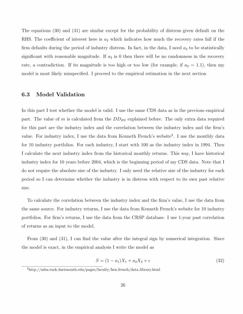
6.3 Model Validation
In this part I test whether the model is valid. I use the same CDS data as in the previous empirical
part. The value of m is calculated from the DDBS explained before. The only extra data required
for this part are the industry index and the correlation between the industry index and the firm’s
value. For industry index, I use the data from Kenneth French’s website2. I use the monthly data
for 10 industry portfolios. For each industry, I start with 100 as the industry index in 1994. Then
I calculate the next industry index from the historical monthly returns. This way, I have historical
industry index for 10 years before 2004, which is the beginning period of my CDS data. Note that I
do not require the absolute size of the industry. I only need the relative size of the industry for each
period so I can determine whether the industry is in distress with respect to its own past relative
size.
To calculate the correlation between the industry index and the firm’s value, I use the data from
the same source. For industry returns, I use the data from Kenneth French’s website for 10 industry
portfolios. For firm’s returns, I use the data from the CRSP database. I use 1-year past correlation
of returns as an input to the model.
From (30) and (31), I can find the value after the integral sign by numerical integration. Since
the model is exact, in the empirical analysis I write the model as
S = (1− a1)X1 + a2X2 + ε (32)
2http://mba.tuck.dartmouth.edu/pages/faculty/ken.french/data library.html
26
where X1 is the first bracket and X2 is the second bracket of the RHS of (30) and (31), and ε is white
noise. With this specification, I can simply estimate a2 by an OLS regression. I select the industry
distress ratio c = 0.8 for the simple model and b = 0.94 for the time-consistent model. The choice of
c = 0.8 has been explained in the previous section. The choice of b = 0.94 is to be consistent with
c = 0.8 in the linear scale. The regression result is shown in Table 10
The results show that the coefficient a2 is highly significant. This means that the expected risk-
neutral recovery rates are lower during the industry distress period. Since the regression is not
separated by industry, this number is an average of all industries. The magnitude of 20% complies
with the literature. Note that this value is the expected decrease of recovery rates in the risk-neutral
measure. It may not correspond exactly to the realized decrease of recovery rates in the physical
measure. The advantage of the model is that it can be used to extract expected recovery rates in
different periods, not relying only on historical data. Overall I conclude that my theoretical model
complies with the data with reasonable parameters.
7 Conclusion and Future Work
Recovery rates have long been treated as a constant. The literature on credit derivatives has focused
mostly on estimating the probability of default. Recently it has been found that the realized recovery
rates are stochastic and highly correlated with the industry condition when the firm defaults. I found
that CDS prices have already incorporated the information on recovery rates. I derive a model for
stochastic recovery rates in CDS spreads, linking unobservable expected recovery rates to observable
industry conditions. This model can be used to extract implied recovery rates in the same way that
default probabilities are extracted from CDS spreads using a particular model.
The paper has two main parts. The first part is the empirical test to identify that stochastic
recovery rates are priced in CDS spreads. The key to separate recovery rates from default probabilities
is the industry characteristics and industry condition, the main driver of realized recovery rates. A
battery of tests are performed to rule out other explanations. In the second part I derive a model
27

for stochastic recovery rates for CDS spreads. I then verify that the model is valid with reasonable
variation of recovery rates across business cycles.
Precise estimation of the cost of default has tremendous implications for fixed-income asset pricing
and capital structure decision in corporate finance. This paper confirms that such information can
be extracted from prevalent CDS data and provides a model which accounts for the stochasticity of
recovery rates. A careful estimation method and fine-tuning parameters of the model are left out for
future research.
28
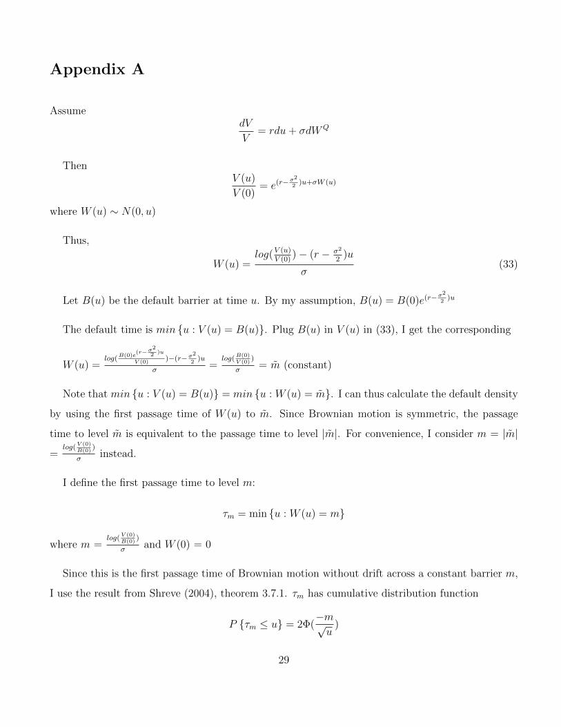
Appendix A
AssumedV
V= rdu+ σdWQ
ThenV (u)
V (0)= e(r−
σ2
2)u+σW (u)
where W (u) ∼ N(0, u)
Thus,
W (u) =log(V (u)
V (0))− (r − σ2
2)u
σ(33)
Let B(u) be the default barrier at time u. By my assumption, B(u) = B(0)e(r−σ2
2)u
The default time is min {u : V (u) = B(u)}. Plug B(u) in V (u) in (33), I get the corresponding
W (u) =log(
B(0)e(r−σ2
2 )u
V (0))−(r−σ
2
2)u
σ=
log(B(0)V (0)
)
σ= m̃ (constant)
Note that min {u : V (u) = B(u)} = min {u : W (u) = m̃}. I can thus calculate the default density
by using the first passage time of W (u) to m̃. Since Brownian motion is symmetric, the passage
time to level m̃ is equivalent to the passage time to level |m̃|. For convenience, I consider m = |m̃|
=log(
V (0)B(0)
)
σinstead.
I define the first passage time to level m:
τm = min {u : W (u) = m}
where m =log(
V (0)B(0)
)
σand W (0) = 0
Since this is the first passage time of Brownian motion without drift across a constant barrier m,
I use the result from Shreve (2004), theorem 3.7.1. τm has cumulative distribution function
P {τm ≤ u} = 2Φ(−m√u
)
29

and density
q(m,u) =d
duP {τm ≤ u} =
m
u√
2πue
−m2
2u
30
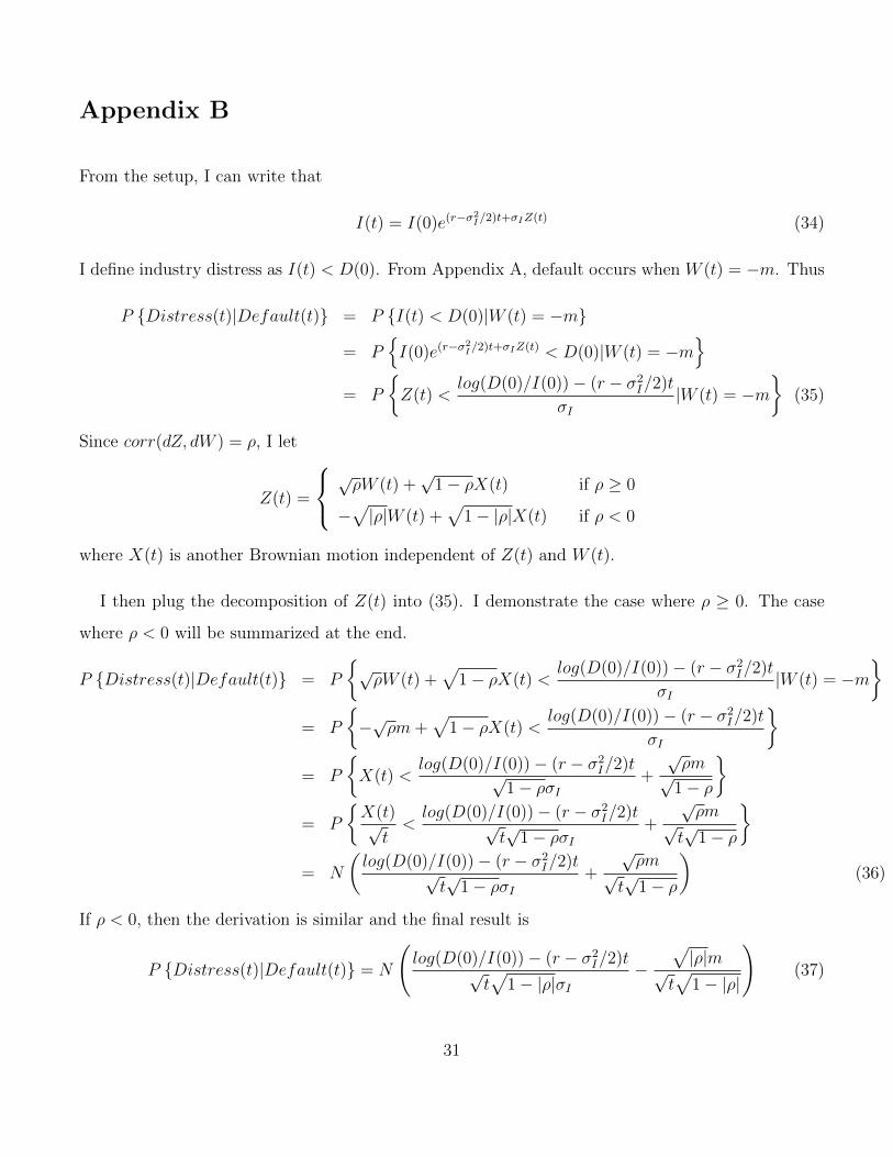
Appendix B
From the setup, I can write that
I(t) = I(0)e(r−σ2I/2)t+σIZ(t) (34)
I define industry distress as I(t) < D(0). From Appendix A, default occurs when W (t) = −m. Thus
P {Distress(t)|Default(t)} = P {I(t) < D(0)|W (t) = −m}
= P{I(0)e(r−σ
2I/2)t+σIZ(t) < D(0)|W (t) = −m
}= P
{Z(t) <
log(D(0)/I(0))− (r − σ2I/2)t
σI|W (t) = −m
}(35)
Since corr(dZ, dW ) = ρ, I let
Z(t) =
√ρW (t) +
√1− ρX(t) if ρ ≥ 0
−√|ρ|W (t) +
√1− |ρ|X(t) if ρ < 0
where X(t) is another Brownian motion independent of Z(t) and W (t).
I then plug the decomposition of Z(t) into (35). I demonstrate the case where ρ ≥ 0. The case
where ρ < 0 will be summarized at the end.
P {Distress(t)|Default(t)} = P
{√ρW (t) +
√1− ρX(t) <
log(D(0)/I(0))− (r − σ2I/2)t
σI|W (t) = −m
}= P
{−√ρm+
√1− ρX(t) <
log(D(0)/I(0))− (r − σ2I/2)t
σI
}= P
{X(t) <
log(D(0)/I(0))− (r − σ2I/2)t√
1− ρσI+
√ρm
√1− ρ
}= P
{X(t)√t<log(D(0)/I(0))− (r − σ2
I/2)t√t√
1− ρσI+
√ρm
√t√
1− ρ
}= N
(log(D(0)/I(0))− (r − σ2
I/2)t√t√
1− ρσI+
√ρm
√t√
1− ρ
)(36)
If ρ < 0, then the derivation is similar and the final result is
P {Distress(t)|Default(t)} = N
(log(D(0)/I(0))− (r − σ2
I/2)t√t√
1− |ρ|σI−
√|ρ|m
√t√
1− |ρ|
)(37)
31
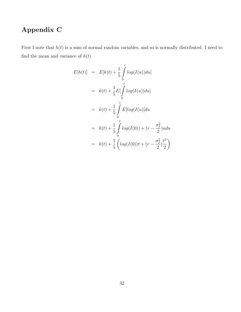
Appendix C
First I note that h(t) is a sum of normal random variables, and so is normally distributed. I need to
find the mean and variance of h(t)
E[h(t)] = E[k(t) +1
5
t∫0
log(I(u))du]
= k(t) +1
5E[
t∫0
log(I(u))du]
= k(t) +1
5
t∫0
E[log(I(u)]du
= k(t) +1
5
t∫0
log(I(0)) + (r − σ2I
2)udu
= k(t) +1
5
(log(I(0))t+ (r − σ2
I
2)t2
2
)
32

V ar[h(t)] = V ar[k(t) +1
5
t∫0
log(I(u))du]
=1
25V ar[
t∫0
log(I(u))du]
=1
25V ar[
t∫0
log(I(0)) + (r − σ2I
2)u+ σIZudu]
=1
25V ar[
t∫0
σIZudu]
=σ2I
25E
t∫0
Zudu
t∫0
Zsds
=
σ2I
25E
t∫0
t∫0
ZuZsduds
=
σ2I
25
t∫0
t∫0
E[ZuZs]duds
=σ2I
25
t∫0
t∫0
min(u, s)duds
=2σ2
I
25
t∫0
s∫0
ududs
=2σ2
I
25
t∫0
s2
2ds
=σ2I
25
t3
3
Having calculated the mean and variance of h(t), I are now ready to calculate the probability of
distress given firm’s default. First I signify h(t) as a normal random variable
h(t) = k(t) +1
5(log(I(0))t+ (r − σ2
I
2)t2
2) +
σI5B(t) (38)
33

where
B(t) ∼ N(0, t3/3)
Then
P {Distress(t)|Default(t)} = P {log(I(t)) < bh(t)|W (t) = −m}
= P
{log(I(0)) + (r − σ2
I
2)t+ σIZ(t) < b
(k(t) +
1
5(log(I(0))t+ (r − σ2
I
2)t2
2) +
σI5B(t)
)|W (t) = −m
}
= P
Z(t) <b(k(t) + 1
5(log(I(0))t+ (r − σ2
I
2) t
2
2
)− log(I(0))− (r − σ2
I
2)t
σI+b
5B(t)|W (t) = −m
Again, I decompose Z(t) into the correlated and uncorrelated parts with the firm. Since corr(dZ, dW ) =
ρ, I let
Z(t) =
√ρW (t) +
√1− ρX(t) if ρ ≥ 0
−√|ρ|W (t) +
√1− |ρ|X(t) if ρ < 0
where X(t) is another Brownian motion independent of Z(t) and W (t).
I carry on the calculation for the case where ρ ≥ 0. The case where ρ < 0 is similar and the result
will be provided at the end. Substituting the decomposition of Z(t) into the previous equation, I get
= P
{√ρW (t) +
√1− ρX(t) <
b(k(t) + 1
5(log(I(0))t+ (r − σ2
I
2) t
2
2
)− log(I(0))− (r − σ2
I
2)t
σI
+b
5B(t)|W (t) = −m
}
= P
−√ρm+√
1− ρX(t) <b(k(t) + 1
5(log(I(0))t+ (r − σ2
I
2) t
2
2
)− log(I(0))− (r − σ2
I
2)t
σI+b
5B(t)
= P
√1− ρX(t) <
(bk(t) + ( bt
5− 1)log(I(0)) + ( bt
2
10− t)(r − σ2
I
2))
σI+√ρm+
b
5B(t)
= P
{√1− ρX(t) < µ(t) +
b
5B(t)
}= P
{√1− ρX(t)− b
5B(t) < µ(t)
}(39)
34

where
µ(t) =
(bk(t) + ( bt
5− 1)log(I(0)) + ( bt
2
10− t)(r − σ2
I
2))
σI+√ρm
Now I note that the LHS of (39) is the difference of two normal random variables, and thus also
normally distributed. I need to find the mean and variance of the random variable on the LHS.
E[√
1− ρX(t)− b
5B(t)] =
√1− ρE[X(t)] +
b
5E[B(t)]
= 0
V ar[√
1− ρX(t)− b
5B(t)] = V ar[
√1− ρX(t)] + V ar[
b
5B(t)]
(X(t) and B(t) are independent)
= t(1− ρ) +b2
25
t3
3
= t(1− ρ) +b2t3
75
With this result, I let
η(t) =√
1− ρX(t)− b
5B(t)
Then η(t) ∼ N(0, t√
1− ρ+ b2t3
75). Thus, I get
P {Distress(t)|Default(t)} = P {η(t) < µ(t)}
= P
η(t)√t(1− ρ) + b2t3
75
<µ(t)√
t(1− ρ) + b2t3
75
= N
µ(t)√t(1− ρ) + b2t3
75
(40)
If ρ < 0, then the derivation is similar and the final result is
µ(t) =
(bk(t) + ( bt
5− 1)log(I(0)) + ( bt
2
10− t)(r − σ2
I
2))
σI−√|ρ|m
and
P {Distress(t)|Default(t)} = N
µ(t)√t(1− |ρ|) + b2t3
75
(41)
35
References
[1] Acharya, Bharath, and Srinivasan. Does industry-wide distress affect defaulted firms? evidence
from creditor recoveries. Journal of Financial Economics, 2007.
[2] V. Acharya and T. Johnson. Insider trading in credit derivatives. Journal of Financial Eco-
nomics, 84, 2007.
[3] Almeida and Philippon. The risk-adjusted cost of financial distress. Journal of Finance, 2007.
[4] Altman, Brady, Resti, and Sironi. The link between default and recovery rates: Theory, empirical
evidence, and implications. Journal of Business, 2005.
[5] E. Altman and V. Kishore. Almost everything you wanted to know about recoveries on defaulted
bonds. Financial Analysts Journal, 52(6):57–64, 1996.
[6] Aunon-Nerin, Cossin, Hricko, and Huang. Exploring for the determinants of credit risk in credit
default swarp transaction data: Is fixed income markets’ information sufficient to evaluate credit
risk? FAME Research Papers, 2002.
[7] Bakshi, Madan, and Zhang. Understanding the role of recovery in default risk models: Empirical
comparisons and implied recovery rates. Working Paper, 2006.
[8] Bharath and Shumway. Forecasting default with the merton distance to default model. Review
of Financial Studies, 2008.
[9] F. Black and J.C. Cox. Valuing corporate securities: Some effects of bond indenture provisions.
Journal of Finance, 1976.
[10] M. Bruche and C. Gonzalez-Aguado. Recovery rates, default probabilities and the credit cycle.
Journal of Banking and Finance, 34, 2010.
[11] Collin-Dufresne and Goldstein. Do credit spreads reflect stationary leverage ratios? Journal of
Finance, 2001.
36
[12] Sanjiv R. Das and Paul Hanouna. Implied recovery. Journal of Economic Dynamics and Control,
33(11):1837 – 1857, 2009.
[13] Sergei A. Davydenko, Ilya A. Strebulaev, and Xiaofei Zhao. A market-based study of the cost
of default. Review of Financial Studies, 25(10):2959–2999, 2012.
[14] Kenneth French. http://mba.tuck.dartmouth.edu/pages/faculty/ken.french/data library.html.
[15] J. Michael Harrison. Brownian Motion and Stochastic Flow Systems. Wiley, 1985.
[16] Hilscher, Pollet, and Wilson. Uninformed and inattentive traders in credit default swap markets.
Working Paper, 2010.
[17] Hull, Predescu, and White. The valuation of correlation-depedent credit derivatives using a
structural model. Working Paper, 2009.
[18] R. Jarrow. Default parameter estimation using market prices. Financial Analysts Journal,
57(5):75–92, 2001.
[19] R. Jarrow and S. Turnbull. The intersection of market and credit risk. Journal of Banking and
Finance, 24, 2000.
[20] Anh Le. Separating the components of default risk: A derivative-based approach. Working
Paper, 2007.
[21] Longstaff, Mithal, and Neis. Corporate yield spreads: Default risk or liquidity? new evidence
from the credit default swaps market. Journal of Finance, 2005.
[22] D. Madan, L. Guntay, and H. Unal. Pricing the risk of recovery in default with absolute priority
rule violation. Journal of Banking and Finance, 27, 2003.
[23] Merton. On the pricing of corporate debt: The risk structure of interest rates. Journal of
Finance, 1974.
[24] Pan and Singleton. Default and recovery implicit in the term structure of sovereign cds spreads.
Journal of Finance, 2008.
37
[25] Standard & Poor’s. Default, transition and recovery: 2008 annual global corporate default study
and rating transitions. Standard & Poor’s Ratings Direct, 2009.
[26] Moody’s Investors Service. The u.s. municipal bond rating scale: Mapping to the global rating
scale and assigning global scale ratings to municipal obligations. Moody’s Rating Methodology,
2007.
[27] Shleifer and Vishny. Liquidation values and debt capacity: A market equilibrium approach.
Journal of Finance, 1992.
[28] Shreve. Stochastic Calculus for Finance II. Springer, 2004.
[29] Zhou. An analysis of default correlations and multiple defaults. Review of Financial Studies,
2001.
38
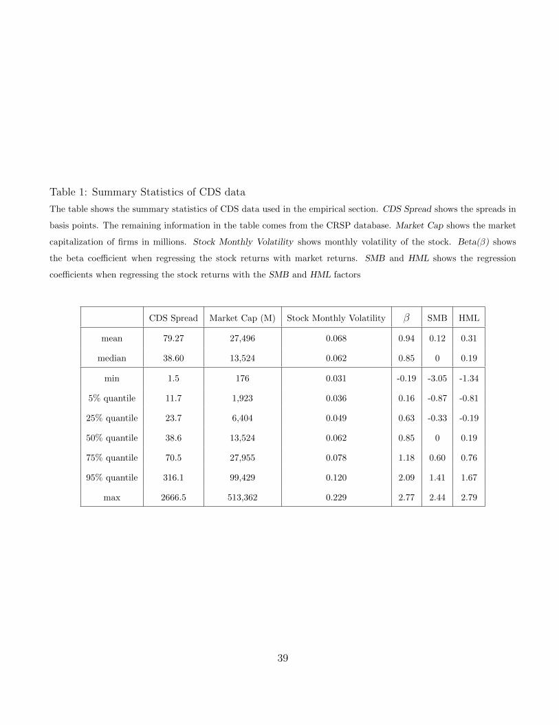
Table 1: Summary Statistics of CDS data
The table shows the summary statistics of CDS data used in the empirical section. CDS Spread shows the spreads in
basis points. The remaining information in the table comes from the CRSP database. Market Cap shows the market
capitalization of firms in millions. Stock Monthly Volatility shows monthly volatility of the stock. Beta(β) shows
the beta coefficient when regressing the stock returns with market returns. SMB and HML shows the regression
coefficients when regressing the stock returns with the SMB and HML factors
CDS Spread Market Cap (M) Stock Monthly Volatility β SMB HML
mean 79.27 27,496 0.068 0.94 0.12 0.31
median 38.60 13,524 0.062 0.85 0 0.19
min 1.5 176 0.031 -0.19 -3.05 -1.34
5% quantile 11.7 1,923 0.036 0.16 -0.87 -0.81
25% quantile 23.7 6,404 0.049 0.63 -0.33 -0.19
50% quantile 38.6 13,524 0.062 0.85 0 0.19
75% quantile 70.5 27,955 0.078 1.18 0.60 0.76
95% quantile 316.1 99,429 0.120 2.09 1.41 1.67
max 2666.5 513,362 0.229 2.77 2.44 2.79
39
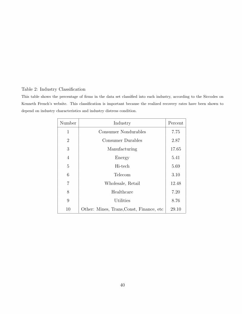
Table 2: Industry Classification
This table shows the percentage of firms in the data set classified into each industry, according to the Siccodes on
Kenneth French’s website. This classification is important because the realized recovery rates have been shown to
depend on industry characteristics and industry distress condition.
Number Industry Percent
1 Consumer Nondurables 7.75
2 Consumer Durables 2.87
3 Manufacturing 17.65
4 Energy 5.41
5 Hi-tech 5.69
6 Telecom 3.10
7 Wholesale, Retail 12.48
8 Healthcare 7.20
9 Utilities 8.76
10 Other: Mines, Trans,Const, Finance, etc 29.10
40

Table 3: Distress cutoff returns for each industry
The table shows the monthly returns below which the industry is in distress. The cutoff level is the 10th percentile of
historical monthly industry returns from 1994 to 2003. The industry returns data are from Kenneth French’s website.
Number Fama-French Industry Distress Cutoff
1 Consumer Nondurables -4.1%
2 Consumer Durables -6.7%
3 Manufacturing -4.6%
4 Energy -4.8%
5 Hi-tech -11.8%
6 Telecom -8.4%
7 Wholesale, Retail -5.0%
8 Healthcare -5.8%
9 Utilities -5.3%
10 Other: Mines, Trans,Const, Finance, etc -5.0%
41
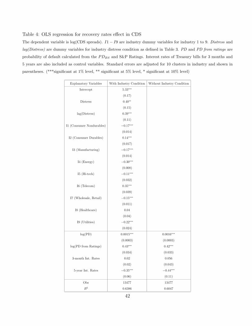
Table 4: OLS regression for recovery rates effect in CDS
The dependent variable is log(CDS spreads). I1− I9 are industry dummy variables for industry 1 to 9. Distress and
lag(Distress) are dummy variables for industry distress condition as defined in Table 3. PD and PD from ratings are
probability of default calculated from the PDBS and S&P Ratings. Interest rates of Treasury bills for 3 months and
5 years are also included as control variables. Standard errors are adjusted for 10 clusters in industry and shown in
parentheses. (***significant at 1% level, ** significant at 5% level, * significant at 10% level)
Explanatory Variables With Industry Condition Without Industry Condition
Intercept 5.33∗∗∗
(0.17)
Distress 0.40∗∗
(0.15)
lag(Distress) 0.39∗∗∗
(0.11)
I1 (Consumer Nondurables) −0.17∗∗∗
(0.014)
I2 (Consumer Durables) 0.14∗∗∗
(0.017)
I3 (Manufacturing) −0.17∗∗∗
(0.014)
I4 (Energy) −0.30∗∗∗
(0.008)
I5 (Hi-tech) −0.11∗∗∗
(0.032)
I6 (Telecom) 0.35∗∗∗
(0.039)
I7 (Wholesale, Retail) −0.15∗∗∗
(0.011)
I8 (Healthcare) 0.04
(0.04)
I9 (Utilities) −0.22∗∗∗
(0.024)
log(PD) 0.0015∗∗∗ 0.0016∗∗∗
(0.0003) (0.0003)
log(PD from Ratings) 0.43∗∗∗ 0.42∗∗∗
(0.034) (0.033)
3-month Int. Rates 0.02 0.056
(0.02) (0.043)
5-year Int. Rates −0.35∗∗∗ −0.44∗∗∗
(0.06) (0.11)
Obs 13477 13477
R2 0.6386 0.6047
42
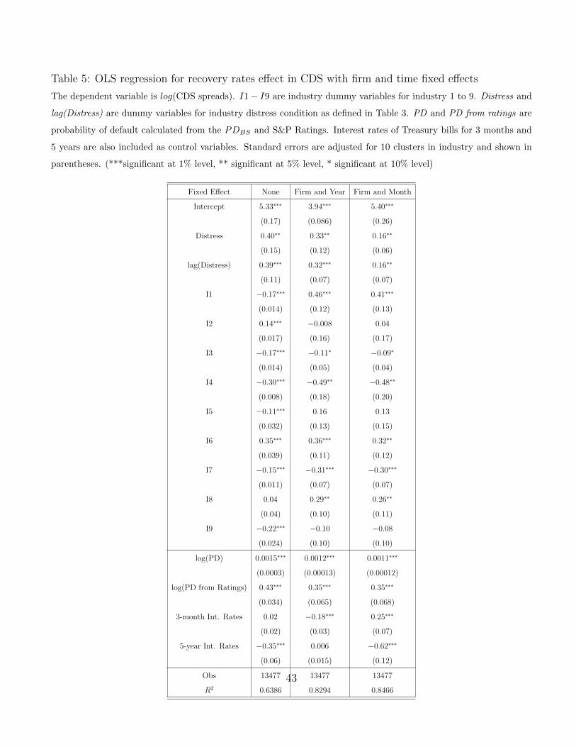
Table 5: OLS regression for recovery rates effect in CDS with firm and time fixed effects
The dependent variable is log(CDS spreads). I1− I9 are industry dummy variables for industry 1 to 9. Distress and
lag(Distress) are dummy variables for industry distress condition as defined in Table 3. PD and PD from ratings are
probability of default calculated from the PDBS and S&P Ratings. Interest rates of Treasury bills for 3 months and
5 years are also included as control variables. Standard errors are adjusted for 10 clusters in industry and shown in
parentheses. (***significant at 1% level, ** significant at 5% level, * significant at 10% level)
Fixed Effect None Firm and Year Firm and Month
Intercept 5.33∗∗∗ 3.94∗∗∗ 5.40∗∗∗
(0.17) (0.086) (0.26)
Distress 0.40∗∗ 0.33∗∗ 0.16∗∗
(0.15) (0.12) (0.06)
lag(Distress) 0.39∗∗∗ 0.32∗∗∗ 0.16∗∗
(0.11) (0.07) (0.07)
I1 −0.17∗∗∗ 0.46∗∗∗ 0.41∗∗∗
(0.014) (0.12) (0.13)
I2 0.14∗∗∗ −0.008 0.04
(0.017) (0.16) (0.17)
I3 −0.17∗∗∗ −0.11∗ −0.09∗
(0.014) (0.05) (0.04)
I4 −0.30∗∗∗ −0.49∗∗ −0.48∗∗
(0.008) (0.18) (0.20)
I5 −0.11∗∗∗ 0.16 0.13
(0.032) (0.13) (0.15)
I6 0.35∗∗∗ 0.36∗∗∗ 0.32∗∗
(0.039) (0.11) (0.12)
I7 −0.15∗∗∗ −0.31∗∗∗ −0.30∗∗∗
(0.011) (0.07) (0.07)
I8 0.04 0.29∗∗ 0.26∗∗
(0.04) (0.10) (0.11)
I9 −0.22∗∗∗ −0.10 −0.08
(0.024) (0.10) (0.10)
log(PD) 0.0015∗∗∗ 0.0012∗∗∗ 0.0011∗∗∗
(0.0003) (0.00013) (0.00012)
log(PD from Ratings) 0.43∗∗∗ 0.35∗∗∗ 0.35∗∗∗
(0.034) (0.065) (0.068)
3-month Int. Rates 0.02 −0.18∗∗∗ 0.25∗∗∗
(0.02) (0.03) (0.07)
5-year Int. Rates −0.35∗∗∗ 0.006 −0.62∗∗∗
(0.06) (0.015) (0.12)
Obs 13477 13477 13477
R2 0.6386 0.8294 0.8466
43
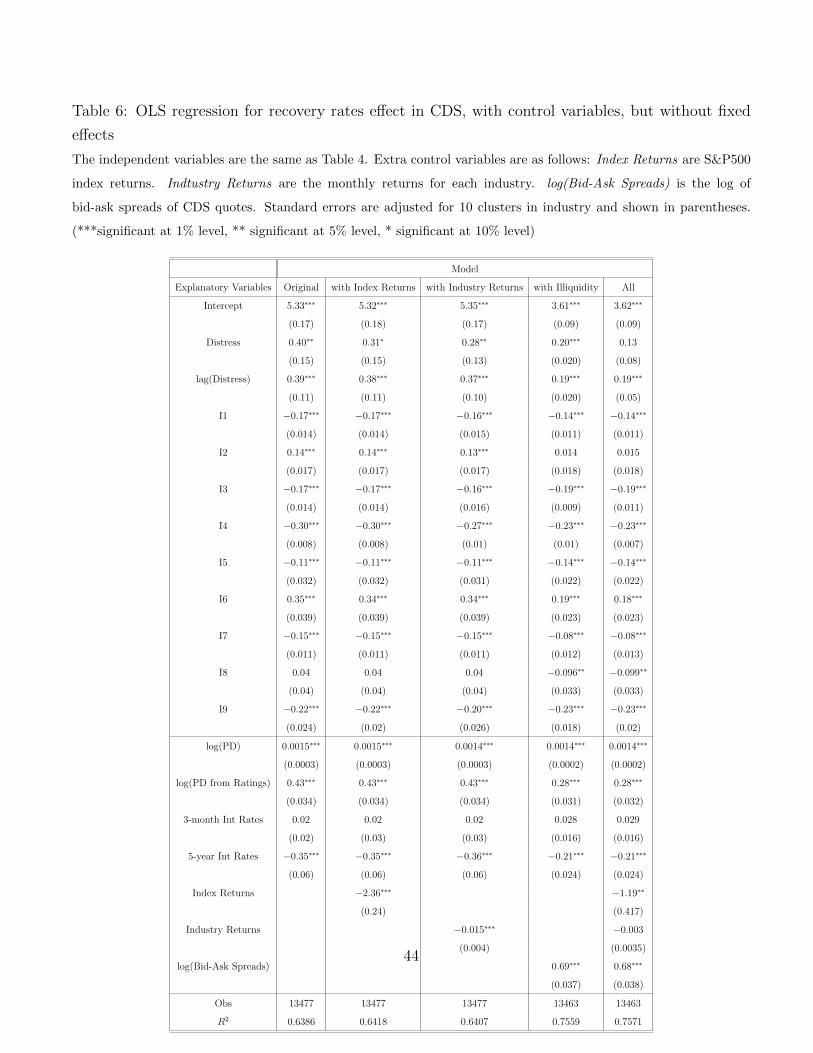
Table 6: OLS regression for recovery rates effect in CDS, with control variables, but without fixed
effects
The independent variables are the same as Table 4. Extra control variables are as follows: Index Returns are S&P500
index returns. Indtustry Returns are the monthly returns for each industry. log(Bid-Ask Spreads) is the log of
bid-ask spreads of CDS quotes. Standard errors are adjusted for 10 clusters in industry and shown in parentheses.
(***significant at 1% level, ** significant at 5% level, * significant at 10% level)
Model
Explanatory Variables Original with Index Returns with Industry Returns with Illiquidity All
Intercept 5.33∗∗∗ 5.32∗∗∗ 5.35∗∗∗ 3.61∗∗∗ 3.62∗∗∗
(0.17) (0.18) (0.17) (0.09) (0.09)
Distress 0.40∗∗ 0.31∗ 0.28∗∗ 0.20∗∗∗ 0.13
(0.15) (0.15) (0.13) (0.020) (0.08)
lag(Distress) 0.39∗∗∗ 0.38∗∗∗ 0.37∗∗∗ 0.19∗∗∗ 0.19∗∗∗
(0.11) (0.11) (0.10) (0.020) (0.05)
I1 −0.17∗∗∗ −0.17∗∗∗ −0.16∗∗∗ −0.14∗∗∗ −0.14∗∗∗
(0.014) (0.014) (0.015) (0.011) (0.011)
I2 0.14∗∗∗ 0.14∗∗∗ 0.13∗∗∗ 0.014 0.015
(0.017) (0.017) (0.017) (0.018) (0.018)
I3 −0.17∗∗∗ −0.17∗∗∗ −0.16∗∗∗ −0.19∗∗∗ −0.19∗∗∗
(0.014) (0.014) (0.016) (0.009) (0.011)
I4 −0.30∗∗∗ −0.30∗∗∗ −0.27∗∗∗ −0.23∗∗∗ −0.23∗∗∗
(0.008) (0.008) (0.01) (0.01) (0.007)
I5 −0.11∗∗∗ −0.11∗∗∗ −0.11∗∗∗ −0.14∗∗∗ −0.14∗∗∗
(0.032) (0.032) (0.031) (0.022) (0.022)
I6 0.35∗∗∗ 0.34∗∗∗ 0.34∗∗∗ 0.19∗∗∗ 0.18∗∗∗
(0.039) (0.039) (0.039) (0.023) (0.023)
I7 −0.15∗∗∗ −0.15∗∗∗ −0.15∗∗∗ −0.08∗∗∗ −0.08∗∗∗
(0.011) (0.011) (0.011) (0.012) (0.013)
I8 0.04 0.04 0.04 −0.096∗∗ −0.099∗∗
(0.04) (0.04) (0.04) (0.033) (0.033)
I9 −0.22∗∗∗ −0.22∗∗∗ −0.20∗∗∗ −0.23∗∗∗ −0.23∗∗∗
(0.024) (0.02) (0.026) (0.018) (0.02)
log(PD) 0.0015∗∗∗ 0.0015∗∗∗ 0.0014∗∗∗ 0.0014∗∗∗ 0.0014∗∗∗
(0.0003) (0.0003) (0.0003) (0.0002) (0.0002)
log(PD from Ratings) 0.43∗∗∗ 0.43∗∗∗ 0.43∗∗∗ 0.28∗∗∗ 0.28∗∗∗
(0.034) (0.034) (0.034) (0.031) (0.032)
3-month Int Rates 0.02 0.02 0.02 0.028 0.029
(0.02) (0.03) (0.03) (0.016) (0.016)
5-year Int Rates −0.35∗∗∗ −0.35∗∗∗ −0.36∗∗∗ −0.21∗∗∗ −0.21∗∗∗
(0.06) (0.06) (0.06) (0.024) (0.024)
Index Returns −2.36∗∗∗ −1.19∗∗
(0.24) (0.417)
Industry Returns −0.015∗∗∗ −0.003
(0.004) (0.0035)
log(Bid-Ask Spreads) 0.69∗∗∗ 0.68∗∗∗
(0.037) (0.038)
Obs 13477 13477 13477 13463 13463
R2 0.6386 0.6418 0.6407 0.7559 0.7571
44

Table 7: OLS regression for recovery rates effect in CDS, with control variables, with fixed effects
The independent variables are the same as Table 4. Extra control variables are as follows: Index Returns are S&P500
index returns. Indtustry Returns are the monthly returns for each industry. log(Bid-Ask Spreads) is the log of
bid-ask spreads of CDS quotes. Standard errors are adjusted for 10 clusters in industry and shown in parentheses.
(***significant at 1% level, ** significant at 5% level, * significant at 10% level)
Fixed Effect
Explanatory Variables None Firm Only Firm and Year Firm and Month
Intercept 3.62∗∗∗ 3.71∗∗∗ 3.00∗∗∗ 4.00∗∗∗
(0.09) (0.18) (0.18) (0.12)
Distress 0.13 0.15∗ 0.14∗ 0.09∗∗
(0.08) (0.08) (0.08) (0.035)
lag(Distress) 0.19∗∗∗ 0.22∗∗∗ 0.20∗∗∗ 0.09∗∗
(0.05) (0.045) (0.03) (0.037)
I1 −0.14∗∗∗ 0.39∗∗∗ 0.43∗∗∗ 0.39∗∗∗
(0.011) (0.05) (0.06) (0.07)
I2 0.015 0.004 0.06 0.09
(0.018) (0.07) (0.11) (0.12)
I3 −0.19∗∗∗ −0.04 −0.03 −0.04
(0.011) (0.06) (0.05) (0.04)
I4 −0.23∗∗∗ −0.19∗∗ −0.32∗∗ −0.33∗∗
(0.007) (0.07) (0.11) (0.13)
I5 −0.14∗∗∗ 0.08 0.07 0.04
(0.022) (0.06) (0.07) (0.09)
I6 0.18∗∗∗ 0.28∗∗ 0.23∗∗ 0.22∗∗
(0.023) (0.10) (0.09) (0.10)
I7 −0.08∗∗∗ −0.20∗∗∗ −0.16∗∗∗ −0.15∗∗
(0.013) (0.06) (0.05) (0.05)
I8 −0.099∗∗∗ 0.33∗∗∗ 0.27∗∗∗ 0.24∗∗
(0.033) (0.09) (0.07) (0.08)
I9 −0.23∗∗∗ −0.02 −0.07 −0.05
(0.02) (0.06) (0.07) (0.07)
log(PD) 0.0014∗∗∗ 0.0010∗∗∗ 0.0010∗∗∗ 0.0010∗∗∗
(0.0002) (0.0002) (0.0001) (0.0001)
log(PD from Ratings) 0.28∗∗∗ 0.28∗∗∗ 0.29∗∗∗ 0.29∗∗∗
(0.032) (0.06) (0.06) (0.06)
3-month Int Rates 0.029 0.03∗ −0.1∗∗∗ 0.20∗∗∗
(0.016) (0.016) (0.02) (0.03)
5-year Int Rates −0.21∗∗∗ −0.25∗∗∗ 0.01∗∗∗ −0.44∗∗∗
(0.024) (0.024) (0.01) (0.044)
Index Returns −1.19∗∗ −1.43∗∗ −1.13∗∗∗ −1.14∗∗∗
(0.417) (0.5) (0.23) (0.27)
Industry Returns −0.003 −0.004 −0.0017 −0.0017
(0.0035) (0.004) (0.0017) (0.002)
log(Bid-Ask Spreads) 0.68∗∗∗ 0.53∗∗∗ 0.50∗∗∗ 0.47∗∗∗
(0.038) (0.07) (0.05) (0.05)
Obs 13463 13463 13463 13463
R2 0.7571 0.8579 0.8684 0.8793
45
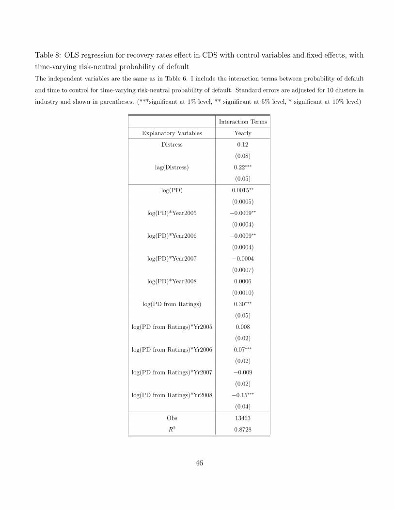
Table 8: OLS regression for recovery rates effect in CDS with control variables and fixed effects, with
time-varying risk-neutral probability of default
The independent variables are the same as in Table 6. I include the interaction terms between probability of default
and time to control for time-varying risk-neutral probability of default. Standard errors are adjusted for 10 clusters in
industry and shown in parentheses. (***significant at 1% level, ** significant at 5% level, * significant at 10% level)
Interaction Terms
Explanatory Variables Yearly
Distress 0.12
(0.08)
lag(Distress) 0.22∗∗∗
(0.05)
log(PD) 0.0015∗∗
(0.0005)
log(PD)*Year2005 −0.0009∗∗
(0.0004)
log(PD)*Year2006 −0.0009∗∗
(0.0004)
log(PD)*Year2007 −0.0004
(0.0007)
log(PD)*Year2008 0.0006
(0.0010)
log(PD from Ratings) 0.30∗∗∗
(0.05)
log(PD from Ratings)*Yr2005 0.008
(0.02)
log(PD from Ratings)*Yr2006 0.07∗∗∗
(0.02)
log(PD from Ratings)*Yr2007 −0.009
(0.02)
log(PD from Ratings)*Yr2008 −0.15∗∗∗
(0.04)
Obs 13463
R2 0.8728
46
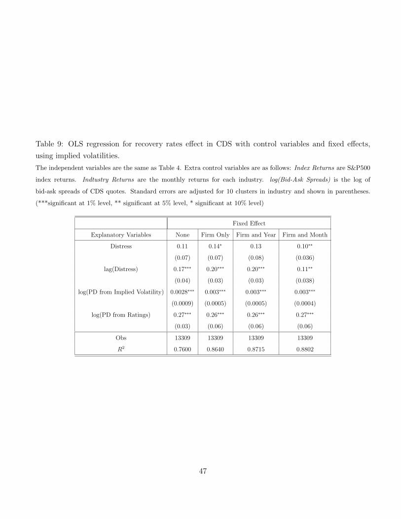
Table 9: OLS regression for recovery rates effect in CDS with control variables and fixed effects,
using implied volatilities.
The independent variables are the same as Table 4. Extra control variables are as follows: Index Returns are S&P500
index returns. Indtustry Returns are the monthly returns for each industry. log(Bid-Ask Spreads) is the log of
bid-ask spreads of CDS quotes. Standard errors are adjusted for 10 clusters in industry and shown in parentheses.
(***significant at 1% level, ** significant at 5% level, * significant at 10% level)
Fixed Effect
Explanatory Variables None Firm Only Firm and Year Firm and Month
Distress 0.11 0.14∗ 0.13 0.10∗∗
(0.07) (0.07) (0.08) (0.036)
lag(Distress) 0.17∗∗∗ 0.20∗∗∗ 0.20∗∗∗ 0.11∗∗
(0.04) (0.03) (0.03) (0.038)
log(PD from Implied Volatility) 0.0028∗∗∗ 0.003∗∗∗ 0.003∗∗∗ 0.003∗∗∗
(0.0009) (0.0005) (0.0005) (0.0004)
log(PD from Ratings) 0.27∗∗∗ 0.26∗∗∗ 0.26∗∗∗ 0.27∗∗∗
(0.03) (0.06) (0.06) (0.06)
Obs 13309 13309 13309 13309
R2 0.7600 0.8640 0.8715 0.8802
47
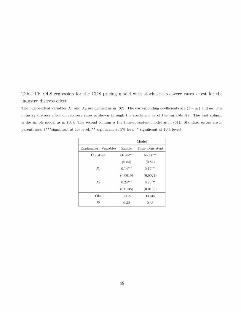
Table 10: OLS regression for the CDS pricing model with stochastic recovery rates - test for the
industry distress effect
The independent variables X1 and X2 are defined as in (32). The corresponding coefficients are (1− a1) and a2. The
industry distress effect on recovery rates is shown through the coefficient a2 of the variable X2. The first column
is the simple model as in (30). The second column is the time-consistent model as in (31). Standard errors are in
parentheses. (***significant at 1% level, ** significant at 5% level, * significant at 10% level)
Model
Explanatory Variables Simple Time-Consistent
Constant 66.45∗∗∗ 66.41∗∗∗
(0.84) (0.84)
X1 0.14∗∗∗ 0.12∗∗∗
(0.0019) (0.0024)
X2 0.24∗∗∗ 0.20∗∗∗
(0.0138) (0.0105)
Obs 14129 14135
R2 0.32 0.33
48
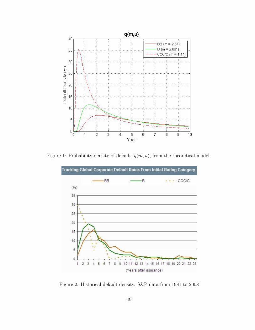
Figure 1: Probability density of default, q(m,u), from the theoretical model
Figure 2: Historical default density. S&P data from 1981 to 2008
49