Thermodynamics education for energy

transformation: a Stirling Engine experiment

Will Yeadon and Mark Quinn

Department of Physics and Astronomy, University of Sheffield, Hounsfield Road,

Sheffield S3 7RH, UK

E-mail: will.yeadon@sheffield.ac.uk

April 2021

Abstract. We present a thermodynamics experiment suitable for first year

undergraduate students employing Stirling Engines to create a demonstration of energy

transformation and to measure the mechanical efficiency of such engines. Using an

inexpensive transparent chambered Stirling Engine, students can connect concepts

such as the theoretical pressure-volume diagram with the physical movements of the

engine’s pistons and the resultant useful output work of a spinning wheel. We found

the majority of students successfully complete this experiment obtaining results similar

to when performed by the authors. In addition to the core thermodynamics lesson,

this experiment incorporates DC circuits, oscilloscopes, and data analysis so it can

be integrated into a wider undergraduate physics course to combine the teaching of

multiple subjects.

1. Introduction

Thermodynamics is a key topic in a contemporary physics degree. Yet core concepts

such as heat and work are often conflated by students [1, 2]. Particularly for process

functions such as work done through pressure and volume changes of a gas, students

may have more difficulty accurately describing the mathematics within a physics context

[3]. Conversely a classical mechanics view of mechanical work being the product of force

and distance is typically introduced to students before university. Novel mental models

and theoretical justifications as methods for teaching thermodynamic concepts has been

the subject of much recent research [4, 5, 6]. Providing an experiment for students to

perform in addition to a theoretical justification enables the conceptualization of energy

transformation to be ”anchored”.

In a review article, Mulop et al. [7] highlighted the difficulty students have in

visualising thermodynamic concepts as a barrier to learning. Stated difficulties included

applying concepts of thermodynamic processes to a real life power plant operation

and theories understood as abstractions that have no real life application. Further,

students typically can hold varied conceptions of energy transformation that are applied

arX

iv:2

105.

0814

2v1

[ph

ysic

s.ed

-ph]

17

May

202

1

Thermodynamics education for energy transformation: a Stirling Engine experiment 2

in different situations: the energy transformation of a ball rolling down a slope is

conceptually different to the energy transformation involved in the forming and breaking

of chemical bonds [8].

The present work presents a possible alleviation of this conceptual barrier as the

thermodynamic process and its resultant output can be ”seen” via the study of an

inexpensive Stirling Engine. Through combining the mechanical work of the gas with

a more familiar classical mechanical view of work students can gain insight into the

transformation of energy. Students also develop and combine multiple competencies

including use of electric circuits, signal detection with oscilloscopes and data analysis.

The following section will detail the thermodynamic principles of Stirling Engines.

Section 3 will provide an overview of the experimental procedure and Section 4 will

present results and analysis to determine the engine’s efficiency.

2. Stirling Engine Thermodynamic Principles

Stirling Engines are heat engines that operate through the cycling of a work fluid through

expansionary and contractionary states to drive pistons that produce useful work. The

expansion and contraction of the gas is driven by exposure to hot and cold plates.

Through measuring the mechanical work of the internal gas and the useful mechanical

work produced, it is possible to calculate the mechanical efficiency of a Stirling Engine.

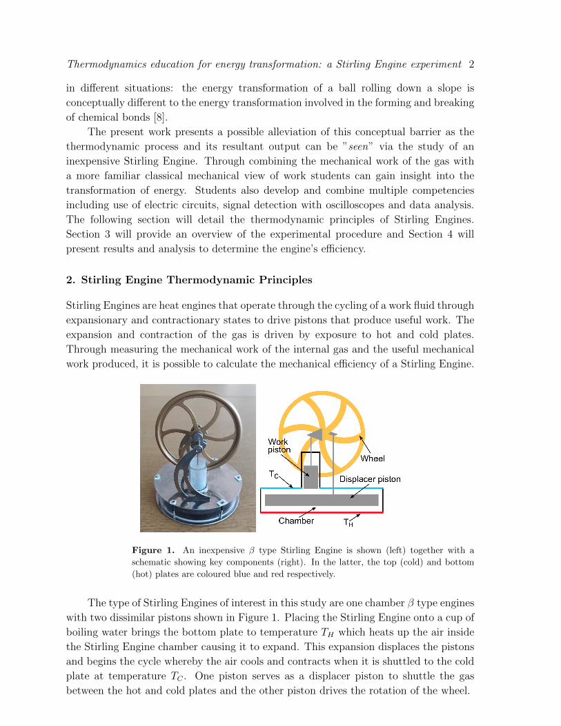
Figure 1. An inexpensive β type Stirling Engine is shown (left) together with a

schematic showing key components (right). In the latter, the top (cold) and bottom

(hot) plates are coloured blue and red respectively.

The type of Stirling Engines of interest in this study are one chamber β type engines

with two dissimilar pistons shown in Figure 1. Placing the Stirling Engine onto a cup of

boiling water brings the bottom plate to temperature TH which heats up the air inside

the Stirling Engine chamber causing it to expand. This expansion displaces the pistons

and begins the cycle whereby the air cools and contracts when it is shuttled to the cold

plate at temperature TC . One piston serves as a displacer piston to shuttle the gas

between the hot and cold plates and the other piston drives the rotation of the wheel.

Thermodynamics education for energy transformation: a Stirling Engine experiment 3

2.1. Pressure - Volume diagram of a Stirling Engine

The development of an analytical model is presented here and is suitable for an early

undergraduate physics course. To begin, we can express the thermodynamic cycle of

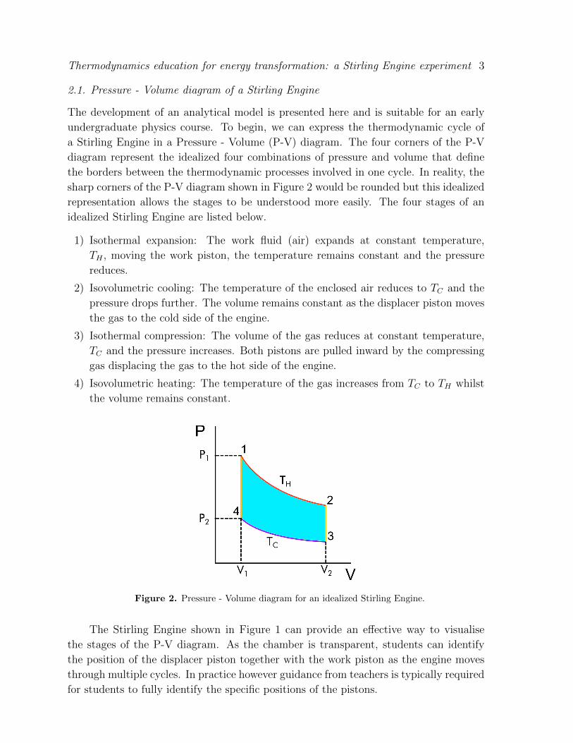
a Stirling Engine in a Pressure - Volume (P-V) diagram. The four corners of the P-V

diagram represent the idealized four combinations of pressure and volume that define

the borders between the thermodynamic processes involved in one cycle. In reality, the

sharp corners of the P-V diagram shown in Figure 2 would be rounded but this idealized

representation allows the stages to be understood more easily. The four stages of an

idealized Stirling Engine are listed below.

1) Isothermal expansion: The work fluid (air) expands at constant temperature,

TH , moving the work piston, the temperature remains constant and the pressure

reduces.

2) Isovolumetric cooling: The temperature of the enclosed air reduces to TC and the

pressure drops further. The volume remains constant as the displacer piston moves

the gas to the cold side of the engine.

3) Isothermal compression: The volume of the gas reduces at constant temperature,

TC and the pressure increases. Both pistons are pulled inward by the compressing

gas displacing the gas to the hot side of the engine.

4) Isovolumetric heating: The temperature of the gas increases from TC to TH whilst

the volume remains constant.

Figure 2. Pressure - Volume diagram for an idealized Stirling Engine.

The Stirling Engine shown in Figure 1 can provide an effective way to visualise

the stages of the P-V diagram. As the chamber is transparent, students can identify

the position of the displacer piston together with the work piston as the engine moves

through multiple cycles. In practice however guidance from teachers is typically required

for students to fully identify the specific positions of the pistons.

Thermodynamics education for energy transformation: a Stirling Engine experiment 4

2.2. Theory

We are interested in determining the mechanical efficiency, η of the Stirling Engine; how

much useful work (W ), is performed by the engine through spinning the wheel compared

to the net work done by the gas. Thus, η can be expressed as

η =Wwheel

Wgas

. (1)

The mechanical work done by the Stirling Engine wheel is defined as its rotational

kinetic energy:

Wwheel = KEwheel =1

2Iω2. (2)

where I is the rotational inertia of the wheel and ω is the angular velocity of the

wheel. We have approximated the wheel as a disk of radius r and mass M with an

angular velocity ω = 2πf . Equation (2) can thus be written as:

Wwheel =1

2

(1

2Mr2

)ω2 =

1

2

(1

2Mr2

)(2πf)2 = Mr2π2f 2. (3)

Next, as depicted in Figure 2, we can express Wgas as the heat entering the cycle in

steps 4 −→ 1 minus the heat leaving the cycle in steps 2 −→ 3. We will assume that the

gas equilibrates with the temperatures TH and TC of the bottom and top plates that

are shown in Figure 1. The work done by the gas is expressed through∫P · dV . Hence

Wgas can be expressed as:

Wgas = W1→2 +W2→3 +W3→4 +W4→1 =

∫P · dV. (4)

However, in steps 4 −→ 1 and 2 −→ 3 the gas changes isochorically (∆V = 0) thus

the work is equal to zero:

W4→1 = W2→3 =

∫P · dV = 0. (5)

In step 1 −→ 2 (3 −→ 4), the pressure and volume change simultaneously during

isothermal expansion (compression). Here equation 5 is 6= 0 and we can use the ideal

gas law, PV = nRT , to derive the work done by the gas. For 1 −→ 2, equation 5 becomes

W1→2 =

∫ V2

V1

P · dV =

∫ V2

V1

nRTHV

· dV = nRTH · lnV2V1

(6)

and in step 3 −→ 4, equation 5 becomes

W3→4 =

∫ V1

V2

P · dV =

∫ V1

V2

nRTCV· dV = nRTC · ln

V1V2. (7)

The gas inside of the Stirling Engine that that performs the work is termed the

work fluid. The ratio of the maximum volume of work fluid, V2, to the minimum volume

Thermodynamics education for energy transformation: a Stirling Engine experiment 5

of the work fluid, V1, is called the compression ration, CR. In the case of the Stirling

Engine we used, shown in Figure 1, this is the ratio of the maximum volume of air

between the plunger and hot plate during the cycle divided by the maximum volume

of air between the plunger and cold plate during the cycle. Using equations 6 and 7,

equation 4 can be written as:

Wgas = W1→2 +W3→4

= nRTH · lnV2V1

+ nRTC · lnV1V2

= nRTH · lnCR + nRTC · ln1

CR

= nR (TH − TC) · lnCR

(8)

The thermal efficiency can be determined using equation 8 as described in Appendix

A. However, for this student investigation, we are interested in the mechanical efficiency.

This can be derived by substituting equations 3 and 8 into equation 1:

η =Mr2π2f 2

nR (TH − TC) · lnCR

. (9)

A final form relevant for the experiment can be written in terms of measured

variables of f and ∆T = TH − TC .

f 2 =nR · lnCR

Mr2π2η∆T. (10)

Hence, equation 9 can be compared to a linear function y = mx + c in completing a

regression analysis to determine the efficiency, η. This is described further in Section 4.

3. Experimental procedure

This experiment requires the following equipment: a Stirling Engine; a light gate, to

measure the engine’s rotation; a breadboard with approximately 10 wires and two 100

Ω resistors; a benchtop power supply; an oscilloscope; two thermocouple probes with

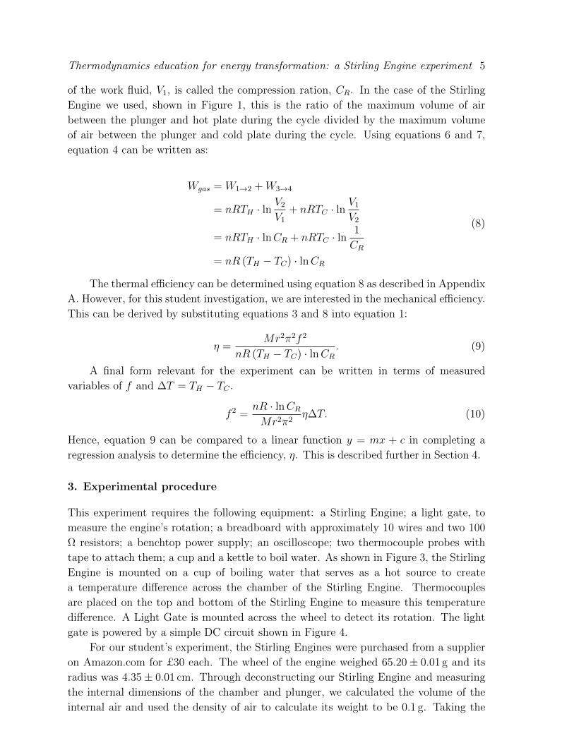
tape to attach them; a cup and a kettle to boil water. As shown in Figure 3, the Stirling

Engine is mounted on a cup of boiling water that serves as a hot source to create

a temperature difference across the chamber of the Stirling Engine. Thermocouples

are placed on the top and bottom of the Stirling Engine to measure this temperature

difference. A Light Gate is mounted across the wheel to detect its rotation. The light

gate is powered by a simple DC circuit shown in Figure 4.

For our student’s experiment, the Stirling Engines were purchased from a supplier

on Amazon.com for £30 each. The wheel of the engine weighed 65.20± 0.01 g and its

radius was 4.35± 0.01 cm. Through deconstructing our Stirling Engine and measuring

the internal dimensions of the chamber and plunger, we calculated the volume of the

internal air and used the density of air to calculate its weight to be 0.1 g. Taking the

Thermodynamics education for energy transformation: a Stirling Engine experiment 6

Figure 3. Experimental setup showing key components and their connections.

Alternatives to equipment such as the oscilloscope and the digital thermometer could

be employed without affecting the experimental outcome.

molar mass of air to be 28.97 g mol−1 we found n in equation 9 to be 3.45 mmol of gas.

Students determine a value of CR by measuring the relevant maximum distances of the

displacement pistons relative to the hot and cold plates. These values describing the

engine are summarised in Table 1.

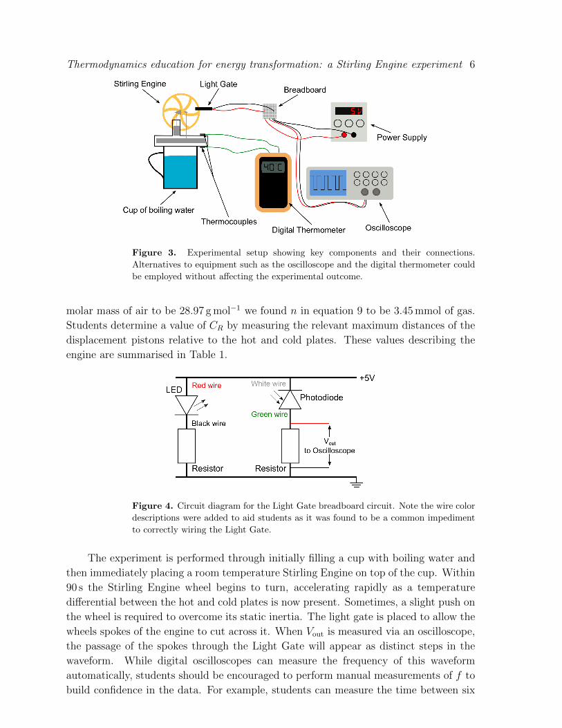
Figure 4. Circuit diagram for the Light Gate breadboard circuit. Note the wire color

descriptions were added to aid students as it was found to be a common impediment

to correctly wiring the Light Gate.

The experiment is performed through initially filling a cup with boiling water and

then immediately placing a room temperature Stirling Engine on top of the cup. Within

90 s the Stirling Engine wheel begins to turn, accelerating rapidly as a temperature

differential between the hot and cold plates is now present. Sometimes, a slight push on

the wheel is required to overcome its static inertia. The light gate is placed to allow the

wheels spokes of the engine to cut across it. When Vout is measured via an oscilloscope,

the passage of the spokes through the Light Gate will appear as distinct steps in the

waveform. While digital oscilloscopes can measure the frequency of this waveform

automatically, students should be encouraged to perform manual measurements of f to

build confidence in the data. For example, students can measure the time between six

Thermodynamics education for energy transformation: a Stirling Engine experiment 7

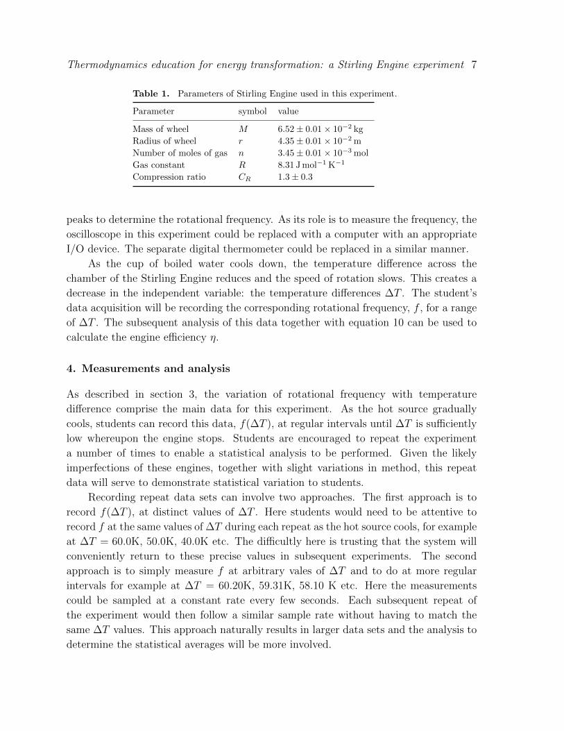
Table 1. Parameters of Stirling Engine used in this experiment.

Parameter symbol value

Mass of wheel M 6.52± 0.01× 10−2 kg

Radius of wheel r 4.35± 0.01× 10−2 m

Number of moles of gas n 3.45± 0.01× 10−3 mol

Gas constant R 8.31 J mol−1 K−1

Compression ratio CR 1.3± 0.3

peaks to determine the rotational frequency. As its role is to measure the frequency, the

oscilloscope in this experiment could be replaced with a computer with an appropriate

I/O device. The separate digital thermometer could be replaced in a similar manner.

As the cup of boiled water cools down, the temperature difference across the

chamber of the Stirling Engine reduces and the speed of rotation slows. This creates a

decrease in the independent variable: the temperature differences ∆T . The student’s

data acquisition will be recording the corresponding rotational frequency, f , for a range

of ∆T . The subsequent analysis of this data together with equation 10 can be used to

calculate the engine efficiency η.

4. Measurements and analysis

As described in section 3, the variation of rotational frequency with temperature

difference comprise the main data for this experiment. As the hot source gradually

cools, students can record this data, f(∆T ), at regular intervals until ∆T is sufficiently

low whereupon the engine stops. Students are encouraged to repeat the experiment

a number of times to enable a statistical analysis to be performed. Given the likely

imperfections of these engines, together with slight variations in method, this repeat

data will serve to demonstrate statistical variation to students.

Recording repeat data sets can involve two approaches. The first approach is to

record f(∆T ), at distinct values of ∆T . Here students would need to be attentive to

record f at the same values of ∆T during each repeat as the hot source cools, for example

at ∆T = 60.0K, 50.0K, 40.0K etc. The difficultly here is trusting that the system will

conveniently return to these precise values in subsequent experiments. The second

approach is to simply measure f at arbitrary vales of ∆T and to do at more regular

intervals for example at ∆T = 60.20K, 59.31K, 58.10 K etc. Here the measurements

could be sampled at a constant rate every few seconds. Each subsequent repeat of

the experiment would then follow a similar sample rate without having to match the

same ∆T values. This approach naturally results in larger data sets and the analysis to

determine the statistical averages will be more involved.

Thermodynamics education for energy transformation: a Stirling Engine experiment 8

20 30 40 50T [K]

1.5

2.0

2.5

3.0

3.5

f [Hz

]

Raw dataBinned mean

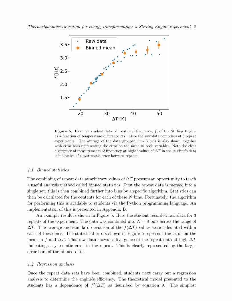
Figure 5. Example student data of rotational frequency, f , of the Stirling Engine

as a function of temperature difference ∆T . Here the raw data comprises of 3 repeat

experiments. The average of the data grouped into 8 bins is also shown together

with error bars representing the error on the mean in both variables. Note the clear

divergence of measurements of frequency at higher values of ∆T in the student’s data

is indicative of a systematic error between repeats.

4.1. Binned statistics

The combining of repeat data at arbitrary values of ∆T presents an opportunity to teach

a useful analysis method called binned statistics. First the repeat data is merged into a

single set, this is then combined further into bins by a specific algorithm. Statistics can

then be calculated for the contents for each of these N bins. Fortunately, the algorithm

for performing this is available to students via the Python programming language. An

implementation of this is presented in Appendix B.

An example result is shown in Figure 5. Here the student recorded raw data for 3

repeats of the experiment. The data was combined into N = 8 bins across the range of

∆T . The average and standard deviation of the f(∆T ) values were calculated within

each of these bins. The statistical errors shown in Figure 5 represent the error on the

mean in f and ∆T . This raw data shows a divergence of the repeat data at high ∆T

indicating a systematic error in the repeat. This is clearly represented by the larger

error bars of the binned data.

4.2. Regression analysis

Once the repeat data sets have been combined, students next carry out a regression

analysis to determine the engine’s efficiency. The theoretical model presented to the

students has a dependence of f 2(∆T ) as described by equation 9. The simplest

Thermodynamics education for energy transformation: a Stirling Engine experiment 9

regression method for students to use here is the least squares approach. Use of this

algorithm is standard in most physics courses and its implementation is available in all

analysis software. To perform the analysis, students equate equation 9 to the linear

function y = mx + c. The algorithm calculates the values of the gradient, m, and the

intercept, c, which best fit the experimental data. The final step is then to use the

gradient value

m =ηnR · lnCRπ2r2M

(11)

together with basic error propagation to determine the engine efficiency η ±∆η.

20 30 40 50 60T [K]

0

5

10

15

20

25

f2 [Hz

2 ]

Student 1Student 2Teacher

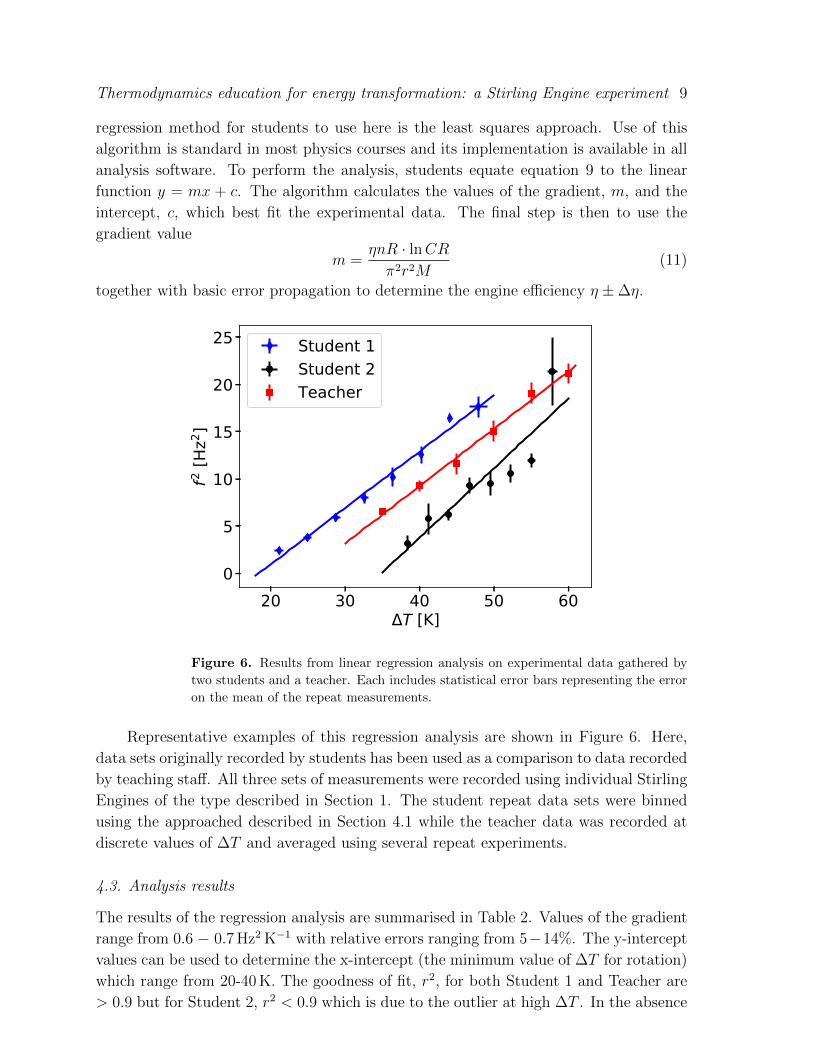
Figure 6. Results from linear regression analysis on experimental data gathered by

two students and a teacher. Each includes statistical error bars representing the error

on the mean of the repeat measurements.

Representative examples of this regression analysis are shown in Figure 6. Here,

data sets originally recorded by students has been used as a comparison to data recorded

by teaching staff. All three sets of measurements were recorded using individual Stirling

Engines of the type described in Section 1. The student repeat data sets were binned

using the approached described in Section 4.1 while the teacher data was recorded at

discrete values of ∆T and averaged using several repeat experiments.

4.3. Analysis results

The results of the regression analysis are summarised in Table 2. Values of the gradient

range from 0.6 − 0.7 Hz2 K−1 with relative errors ranging from 5−14%. The y-intercept

values can be used to determine the x-intercept (the minimum value of ∆T for rotation)

which range from 20-40 K. The goodness of fit, r2, for both Student 1 and Teacher are

> 0.9 but for Student 2, r2 < 0.9 which is due to the outlier at high ∆T . In the absence

Thermodynamics education for energy transformation: a Stirling Engine experiment 10

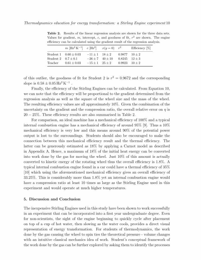
Table 2. Results of the linear regression analysis are shown for the three data sets.

Values for gradient, m, intercept, c, and goodness of fit, r2 are shown. The engine

efficiency can be calculated using the gradient result of the regression analysis.

m [Hz2 K−1] c [Hz2] x(y = 0) r2 Efficiency [%]

Student 1 0.60± 0.03 −11± 1 18± 2 0.9877 10± 2

Student 2 0.7± 0.1 −26± 7 40± 10 0.8245 12± 3

Teacher 0.61± 0.03 −15± 1 25± 2 0.9923 10± 2

of this outlier, the goodness of fit for Student 2 is r2 = 0.9672 and the corresponding

slope is 0.58± 0.05 Hz2 K−1 .

Finally, the efficiency of the Stirling Engines can be calculated. From Equation 10,

we can note that the efficiency will be proportional to the gradient determined from the

regression analysis as well as the square of the wheel size and the mass of the wheel.

The resulting efficiency values are all approximately 10%. Given the combination of the

uncertainty on the gradient and the compression ratio, the overall relative error on η is

20− 25%. These efficiency results are also summarised in Table 2.

For comparison, an ideal machine has a mechanical efficiency of 100% and a typical

internal combustion engine has a mechanical efficiency of around 95% [9]. Thus a 10%

mechanical efficiency is very low and this means around 90% of the potential power

output is lost to the surroundings. Students should also be encouraged to make the

connection between this mechanical efficiency result and the thermal efficiency. The

latter can be generously estimated as 18% by applying a Carnot model as described

in Appendix A. Hence, a maximum of 18% of the initial heat energy can be converted

into work done by the gas for moving the wheel. Just 10% of this amount is actually

converted to kinetic energy of the rotating wheel thus the overall efficiency is 1.8%. A

typical internal combustion engine found in a car could have a thermal efficiency of 35%

[10] which using the aforementioned mechanical efficiency gives an overall efficiency of

33.25%. This is considerably more than 1.8% yet an internal combustion engine would

have a compression ratio at least 10 times as large as the Stirling Engine used in this

experiment and would operate at much higher temperatures.

5. Discussion and Conclusion

The inexpensive Stirling Engines used in this study have been shown to work successfully

in an experiment that can be incorporated into a first year undergraduate degree. Even

for non-scientists, the sight of the engine beginning to quickly cycle after placement

on top of a cup of hot water, then slowing as the water cools, provides a direct visual

representation of energy transformation. For students of thermodynamics, the work

done by the gas causing the wheel to spin ties the theoretical pressure - volume changes

with an intuitive classical mechanics idea of work. Student’s conceptual framework of

the work done by the gas can be further explored by asking them to identify the processes

Thermodynamics education for energy transformation: a Stirling Engine experiment 11

listed in Section 2.1 with the individual strokes of the Stirling Engine’s pistons during

one full cycle.

This experiment can also be integrated into wider experimental skills development.

For example, prior sessions can be devoted to developing competence with DC circuits,

motion sensing and signal measurement via oscilloscopes. The subsequent engine

experiment can then incorporate these individually developed skills to build and carry

out an experimental investigation. Further skills development including merging repeat

data and performing statistical data analysis can follow on from the experimental

session. This multi-session approach was the case for the student cohorts who performed

this experiment at the author’s institution.

In teaching this experiment with two first year undergraduate cohorts, the vast

majority complete the experiment within three hours. However, there are some regular

issues students encountered with the experiment. A typical problem was the wheel not

moving as the plates heat up. This is solved simply by giving the wheel a slight push to

overcome the static inertia. Students may also struggle wiring up the Light Gate circuit

shown in Figure 4. We found that explicitly showing the wire colors on the figure used in

the lab handout and emphasizing to students to beware of inadvertent contact between

circuit components helped with this.

Occasionally, after some use, the Stirling Engines would seize up and either not cycle

or cycle slowly despite an obviously large temperature difference. This can be solved by

taking the wheel off and pulling the smaller piston completely out its containment tube.

After this, upon reassembly the Stirling Engine performs as normal. We speculate this is

due to air gradually being forced out of the central engine chamber as the pistons cycle

which alters the pressure inside the chamber. Another cause of slow cycling occurs when

the Stirling Engine wheel spins slightly off-axis creating a fishtail motion. The solution

here is to alter the axis alignment by wiggling the wheel and bending the support arms

inwards to secure the wheel better.

To improve performance of the Stirling Engines, optional modifications can be

added. Lubricant can be applied to the pin bearings and piston rods to ease their

movement and thermal insulation can be added to achieve a higher ∆T across the top

and bottom plates. Looking closely at the top plate in the photo on the left of Figure

1 reveals the thermal insulation modification. Whilst this is a large amount of work

for multiple engines, this modification provides a strong performance improvement with

peak ∆T > 65 K and a slower reduction in temperature difference compared to without

the modification.

Due to ∆T being a temperature difference, it is possible to drive the Stirling Engine

through a colder TC rather than a hotter TH . This can be achieved though setting the

Stirling Engine on a Petri dish full of dry ice to cool the bottom plate to around −70 °C.

Hence with the top plate at room temperature, a higher maximum ∆T ≈ 90 K can be

achieved. However, thermal conduction will also gradually cool the top plate reducing

the ∆T until the wheel slows to a stop. Interestingly, placing the dry ice on the top

plate of the Stirling Engine will cause the wheel to spin in the opposite direction as the

Thermodynamics education for energy transformation: a Stirling Engine experiment 12

TC and TH plates are ”flipped”. However, the advantage of placing the Stirling Engines

on top of dry ice is that the teacher can prepare this more easily so the students do not

have to handle the dry ice.

To conclude, the thermodynamics experiment described in this paper is a valuable

addition to an undergraduate first year physics course. The experiment provides

students the opportunity to connect thermodynamic process functions with physical

movements of a wheel creating a conceptual framework for work. Students are exposed

to oscilloscopes, DC circuits and light gates creating a thorough experience in physics

experimentation. Further, the regression analysis and use of binned statistics provides

students with a gentle introduction into data analysis.

Acknowledgments

We are grateful to Dr. Stephen Collins and Richard Webb for their technical support

and to Jennifer Bartlett for assisting with the initial conception of this experiment. We

also wish to thank the ShePHERD group for contributing to the final proofing of this

article.

Appendix A. Thermal efficiency

The student experiment described in the main paper aims to determine the mechanical

efficiency of the Stirling Engine - the useful work divided by the outputted work.

However, to determine the thermal efficiency the work done on the system must be

evaluated. This can be found through transforming equation 5, and therefore equation

8, into

Woutput = −∫P · dV = −nR(TH − TC) · lnCR. (A.1)

The heat inputted into the system comes from the hot plate QH = TH∆S. Using

the first law of thermodynamics and equation 6 we find QH to be

QH = −nRTH · lnCR. (A.2)

Through combining equations A.1 and A.2 the Carnot efficiency can thus be

recovered

η =W

QH

=−nR(TH − TC) · lnCR−nRTH · lnCR

= 1− TCTH

(A.3)

The maximum Carnot efficiency, using a ∆T = 65 K and TH = 85 °C is around 18%.

However our simplified view does not take into account the additional terms included

in QH such as regenerative heat loss

Qr = MCV (1− εr)(TH − TC) (A.4)

Thermodynamics education for energy transformation: a Stirling Engine experiment 13

Where M is the molar mass of the work fluid, CV the molar specific heat capacity

at constant volume of the work fluid and εr is the regenerator effectiveness. A.4 would

thus have to be included in the denominator in equation A.3 meaning we will not reach

the Carnot efficiency. For a more detailed breakdown, see [11].

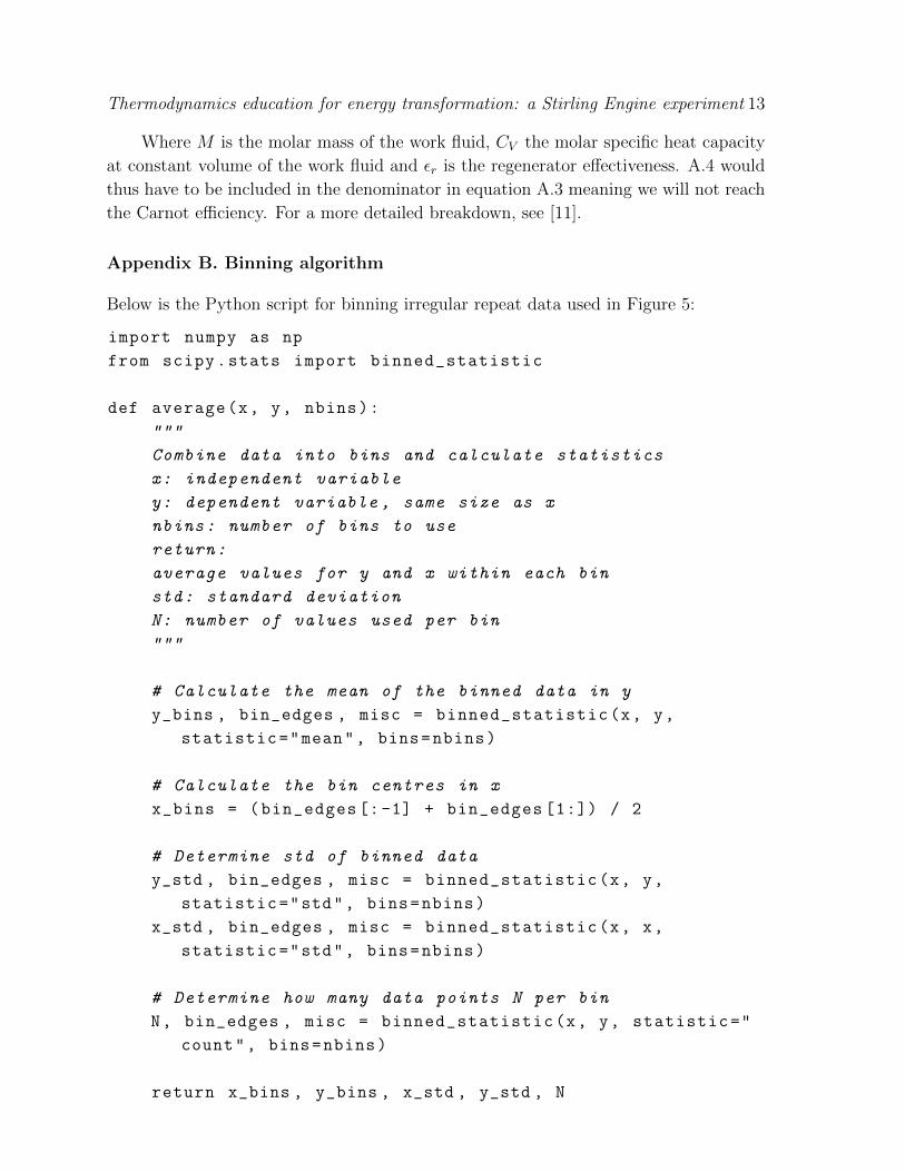
Appendix B. Binning algorithm

Below is the Python script for binning irregular repeat data used in Figure 5:

import numpy as np

from scipy.stats import binned_statistic

def average(x, y, nbins):

"""

Combine data into bins and calculate statistics

x: independent variable

y: dependent variable , same size as x

nbins: number of bins to use

return:

average values for y and x within each bin

std: standard deviation

N: number of values used per bin

"""

# Calculate the mean of the binned data in y

y_bins , bin_edges , misc = binned_statistic(x, y,

statistic="mean", bins=nbins)

# Calculate the bin centres in x

x_bins = (bin_edges [:-1] + bin_edges [1:]) / 2

# Determine std of binned data

y_std , bin_edges , misc = binned_statistic(x, y,

statistic="std", bins=nbins)

x_std , bin_edges , misc = binned_statistic(x, x,

statistic="std", bins=nbins)

# Determine how many data points N per bin

N, bin_edges , misc = binned_statistic(x, y, statistic="

count", bins=nbins)

return x_bins , y_bins , x_std , y_std , N

REFERENCES 14

References

[1] David E. Meltzer. “Investigation of students’ reasoning regarding heat, work,

and the first law of thermodynamics in an introductory calculus-based general

physics course”. In: American Journal of Physics 72.11 (2004), pp. 1432–1446.

doi: 10.1119/1.1789161. eprint: https://doi.org/10.1119/1.1789161. url:

https://doi.org/10.1119/1.1789161.

[2] P. H. van Roon, H. F. van Sprang, and A. H. Verdonk. “‘Work’ and ‘Heat’: on a

road towards thermodynamics”. In: International Journal of Science Education

16.2 (1994), pp. 131–144. doi: 10 . 1080 / 0950069940160203. eprint: https :

//doi.org/10.1080/0950069940160203. url: https://doi.org/10.1080/

0950069940160203.

[3] Evan B. Pollock, John R. Thompson, and Donald B. Mountcastle. “Student

Understanding Of The Physics And Mathematics Of Process Variables In P-

V Diagrams”. In: AIP Conference Proceedings 951.1 (2007), pp. 168–171. doi:

10.1063/1.2820924.

[4] Joon-Hwi Kim and Juno Nam. “Thermodynamic identities with sunray diagrams”.

In: European Journal of Physics 42.3 (Mar. 2021), p. 035101. doi: 10.1088/1361-

6404/abce1e. url: https://doi.org/10.1088/1361-6404/abce1e.

[5] Trevor C. Lipscombe and Carl E. Mungan. “Breathtaking Physics: Human

Respiration as a Heat Engine”. In: The Physics Teacher 58.3 (2020), pp. 150–

151. doi: 10.1119/1.5145400. eprint: https://doi.org/10.1119/1.5145400.

url: https://doi.org/10.1119/1.5145400.

[6] Guobin Wu and Amy Yimin Wu. “A new perspective of how to understand entropy

in thermodynamics”. In: Physics Education 55.1 (Nov. 2019), p. 015005. doi: 10.

1088/1361-6552/ab4de6. url: https://doi.org/10.1088/1361-6552/ab4de6.

[7] Normah Mulop, Khairiyah Mohd Yusof, and Zaidatun Tasir. “A Review on

Enhancing the Teaching and Learning of Thermodynamics”. In: Procedia -

Social and Behavioral Sciences 56 (2012). International Conference on Teaching

and Learning in Higher Education in conjunction with Regional Conference

on Engineering Education and Research in Higher Education, pp. 703–712.

issn: 1877-0428. doi: https : / / doi . org / 10 . 1016 / j . sbspro . 2012 . 09 .

706. url: https : / / www . sciencedirect . com / science / article / pii /

S1877042812041687.

[8] Michael Macrie-Shuck and Vicente Talanquer. “Exploring Students’ Explanations

of Energy Transfer and Transformation”. In: Journal of Chemical Education 97.12

(2020), pp. 4225–4234. doi: 10.1021/acs.jchemed.0c00984. eprint: https:

//doi.org/10.1021/acs.jchemed.0c00984. url: https://doi.org/10.1021/

acs.jchemed.0c00984.

REFERENCES 15

[9] Mostafa A. ElBahloul, ELsayed S. Aziz, and Constantin Chassapis. “Mechanical

efficiency prediction methodology of the hypocycloid gear mechanism for internal

combustion engine application”. In: International Journal on Interactive Design

and Manufacturing 13 (Mar. 2019), pp. 221–233. issn: 1955-2505. doi: 10.1007/

s12008-018-0508-2. url: https://doi.org/10.1007/s12008-018-0508-2.

[10] Jerald A Caton. “Maximum efficiencies for internal combustion engines:

Thermodynamic limitations”. In: International Journal of Engine Research 19.10

(2018), pp. 1005–1023. doi: 10 . 1177 / 1468087417737700. eprint: https : / /

doi.org/10.1177/1468087417737700. url: https://doi.org/10.1177/

1468087417737700.

[11] Mohammad Hossein Ahmadi, Mohammad Ali Ahmadi, and Mehdi Mehrpooya.

“Investigation of the effect of design parameters on power output and thermal

efficiency of a Stirling engine by thermodynamic analysis”. In: International

Journal of Low-Carbon Technologies 11.2 (May 2016), pp. 141–156. issn: 1748-

1317. doi: 10.1093/ijlct/ctu030. eprint: https://academic.oup.com/ijlct/

article-pdf/11/2/141/6766247/ctu030.pdf. url: https://doi.org/10.

1093/ijlct/ctu030.