Embed Size (px)
Citation preview

UCGE Reports Number 20202
Department of Geomatics Engineering
Mitigation of Narrow Band Interference on Software Receivers based on Spectrum Analysis
(URL: http://www.geomatics.ucalgary.ca/links/GradTheses.html)
by
Zhi Jiang October 2004
THE UNIVERSITY OF CALGARY
Mitigation of Narrow Band Interference on Software Receivers based on Spectrum Analysis
by
Zhi Jiang
A THESIS
SUBMITTED TO THE FACULTY OF GRADUATE STUDIES IN PARTIAL FULFILMENT OF THE REQUIREMENTS FOR THE
DEGREE OF MASTER OF SCIENCE
DEPARTMENT OF GEOMATICS ENGINEERING
CALGARY, ALBERTA
October, 2004
© Zhi Jiang 2004

iii
Abstract
This thesis describes an extensive investigation into the development of a
narrow-band radio frequency interference (RFI) mitigation algorithm and
performance testing using a software Global Positioning System (GPS) receiver.
Traditionally, most RFI mitigation methods have been implemented and tested
using conventional hardware receivers. With the rapid development of computer
technologies, the signal processing computational load is becoming less of a
concern, and thus it becomes feasible to develop and test new interference
mitigation methods based on software receivers together with modern digital
signal processing techniques.
In this research, a narrow-band RFI mitigation algorithm based on spectrum
analysis is discussed in the acquisition, tracking and position domains. A series of
hardware simulation tests is conducted to assess the performance of this
algorithm. For high level interference, a fixed detection threshold as previously
suggested in the literature is not sufficient. An adaptive detection threshold that is
a function of the standard deviation of the normalized spectrum and the correlator
power output is proposed in this research. Soft thresholding in bit synchronization
and improved acquisition based on earlier information are used under high
dynamic conditions and a high level interference environment. The factors that
are crucial for weak signal detection (namely coherent integration time, tracking
iv
loop bandwidth and integration time in the loop filter) are evaluated to assess the
effectiveness of this algorithm. Some interference suppression strategies for
spread spectrum systems, namely windowing and overlap processing, are also
investigated. The result shows that the frequency excision algorithm is effective to
mitigate a certain power level of narrow-band RFI, including CW, AM and FM.
Windowing and overlapped processing have shown to be good strategies to
improve the performance of this algorithm by increasing anti-jamming capability
by 2 dB.

v
Acknowledgements
I would like to express my sincere appreciation to my supervisor, Dr. Gérard
Lachapelle, for his continued guidance, encouragement and financial support
throughout my graduate studies. Beyond sharing his knowledge, lessons I have
learned from his positive attitude, spirit of cooperation and understanding will
benefit me throughout my life.
I would also like to thank other professors, students, and staff of the Department
of Geomatics Engineering. Specifically, thank Dr. Changlin Ma for many of his
ideas that have been implemented in this work. I would also like to express
gratitude to Sameet M. Deshpande for his valuable comments and proofreading
of my thesis. Dr. Mark Petovello, Bo Zheng, Haitao Zhang, Lei Dong and Ping
Lian are also thanked for their kind help during my research.
A special recognition and thanks is given to my wife, Yan, for always believing in
me and supporting me. Thank you for your patience, love and understanding. To
my son, Chaofan, thank you for bringing me so much joy and making my life
colourful. I am also indebted to my parents and parents-in-law for their untiring
support.

vi
Table of Contents
Approval Page ………………………………………………………. ……ii Abstract...............................................................................................iii Acknowledgements............................................................................. v
Table of Contents .............................................................................. vi List of Tables ..................................................................................... ix
List of Figures ..................................................................................... x
List of Abbreviations .........................................................................xiii 1 Introduction ...................................................................................1
1.1 Background.............................................................................................. 2 1.1.1 Software receiver versus hardware receiver...................................... 2 1.1.2 Interference overview ........................................................................ 3
1.2 Literature review ...................................................................................... 5 1.3 Research objectives................................................................................. 8 1.4 Thesis outline........................................................................................... 9
2 Theory of FFT-based Narrow-band Interference Excision and Introduction to Receiver Technology ................................................10
2.1 Narrow-band versus wide-band interference............................................. 10 2.2 Fast Fourier Transform.............................................................................. 12 2.3 Algorithm for FFT-based narrow-band interference mitigation................... 15 2.4 Introduction to GPS receiver technology ................................................... 20
2.4.1 GPS signal acquisition overview ......................................................... 20 2.4.2 GPS signal tracking overview.............................................................. 24 2.4.3 Raw measurement derivation.............................................................. 28 2.4.4 Loop filter determination...................................................................... 30
3 Test Setup and Methodology ......................................................35
3.1 RF GPS signal with interference generation .......................................... 35 3.1.1 GSS STR6560 multi-channel GPS/SBAS simulator........................ 35

vii
3.1.2 Interference generation combined with GPS signal ......................... 36 3.2 Intermediate frequency signal generation, sampling and....................... 39 quantization ............................................................................................ 39 3.3 Metrics definition.................................................................................... 40 3.4 Software approach of FFT-based mitigation algorithm........................... 43
3.4.1 Interference detection ...................................................................... 44 3.4.2 Interference mitigation ..................................................................... 46
4 Mitigation Analysis in Acquisition ................................................52
4.1 CW Interference frequency determination ............................................. 52 4.2 Impact of CW interference on correlation function ................................. 55
4.2.1 CW frequency effect on correlation function .................................... 55 4.2.2 CW power effect on correlation function .......................................... 56
4.3 Mitigation result using a 4.75 MHz sampling rate .................................. 58 4.4 Mitigation result using a 7 MHz sampling rate ....................................... 64 4.5 Nyquist’s law and analysis of sampling rate on acquisition.................... 66
4.5.1 Nyquist’s law.................................................................................... 66 4.5.2 Analysis of sampling rate on acquisition .......................................... 68
4.6 Influence of coherent integration time on interference mitigation........... 69 4.7 Conclusion ............................................................................................. 72
5 Mitigation Analysis in Tracking and Position ...............................73
5.1 CW interference mitigation results in tracking........................................ 73 5.1.1 IP component mitigation results....................................................... 73 5.1.2 Doppler mitigation results ................................................................ 76 5.1.3 Estimated C/N0 ................................................................................ 80
5.2 CW Interference mitigation results in position domain ........................... 83 5.2.1 Bench marks for performance analysis in position domain.............. 83 5.2.2 Warm and cold start......................................................................... 85 5.2.3 CW interference mitigation in the position domain........................... 86 5.2.4 Stochastic repeatability test ............................................................. 90
5.3 AM interference mitigation results in the position domain ...................... 94 5.4 FM interference mitigation results in the position domain .................... 100
6 Kinematic Tests.........................................................................109
6.1 Test setup............................................................................................. 109 6.2 Results and analysis ............................................................................ 109

viii
7 Application of Data Window in FFT-based Mitigation Algorithm123
7.1 The advantage of using a data window................................................ 123 7.2 Window selection ................................................................................. 125
7.2.1 Blackman-Harris window ............................................................... 126 7.2.2 Hamming window .......................................................................... 128 7.2.3 Gaussian window........................................................................... 129
7.3 Implementation of overlapped processing ........................................... 131 7.4 Results and analysis ............................................................................ 133
8 Conclusions and Recommendations for Future Work...............142
8.1 Conclusions ......................................................................................... 142 8.2 Recommendations for future work ....................................................... 145
References .....................................................................................147

ix
List of Tables
Table 1.1: Types and sources of jamming interference .................................. 4
Table 2.1: Loop Filter Characteristics ........................................................... 32
Table 3.1: Decision statistic results summary ............................................... 46
Table 4.1: Worst C/A line for each of the 37 codes....................................... 54
Table 4.2: Peak value versus noise floor and SNR ...................................... 63
Table 5.1: Frequency limits versus centre frequency.................................. 102
Table 5.2: Comparison of FM frequency on GPS position.......................... 103
Table 6.1: Impact of integration time in loop filters on position errors ......... 110

x
List of Figures
Figure 2.1: GPS signal acquisition ............................................................... 21
Figure 2.2: GPS receiver signal tracking loop .............................................. 25
Figure 2.3: Software Receiver Delay lock loop............................................. 27
Figure 2.4: Pseudorange construction [after Ward 1996] ............................. 29
Figure 2.5: Second order loop filter .............................................................. 33
Figure 2.6: Digital representation of Laplace transform................................ 34
Figure 3.1: System hardware configuration.................................................. 38
Figure 3.2: Hardware front-end “GPS Signal Tap”........................................ 40
Figure 3.3: Sky view at the beginning of the simulation................................ 43
Figure 3.4: 1 ms FFT without CW interference............................................. 48
Figure 3.5: 1 ms FFT with CW interference (J/S = 30 dB)............................ 48
Figure 3.6: Flowchart of frequency excision algorithm ................................. 51
Figure 4.1: Spectrum of Gold code [from Heppe, 2002] ............................... 52
Figure 4.2: Correlations for different spectral lines ....................................... 55
Figure 4.3: Correlation for CW interference of different power levels ........... 57
Figure 4.4: Acquisition results without mitigation .......................................... 58
Figure 4.5: PDF of noise and signal used in computation of noise power [after
Kaplan, 1996]: ....................................................................................... 60
Figure 4.6: Acquisition results with mitigation at a 4.75 MHz sampling rate . 62
Figure 4.7: Acquisition results with mitigation at a 7 MHz sampling rate ...... 65

xi
Figure 4.8: Spectrum aliasing....................................................................... 67
Figure 4.9: Impact of coherent time on mitigation results ............................. 71
Figure 5.1: IP component comparison.......................................................... 74
Figure 5.2: Comparison of Doppler with 4.75 MHz sampling rate ................ 76
Figure 5.3: Comparison of Doppler with 7 MHz sampling rate ..................... 76
Figure 5.4: Doppler error comparison (5 seconds of data) ........................... 78
Figure 5.5: Doppler error comparison (30 seconds of data) ......................... 79
Figure 5.6: C/N0 comparison ........................................................................ 82
Figure 5.7: Position errors under noise only conditions................................ 83
Figure 5.8: Position error comparison of 6 tests under noise only conditions
.............................................................................................................. 84
Figure 5.9: Comparison of mitigation results with CW interference .............. 87
Figure 5.10: Comparison of the effect of the sampling rate on position........ 89
Figure 5.11: Comparison of coherent integration time on position................ 91
Figure 5.12: Rate of successful position fixing ............................................. 93
Figure 5.13: Impact of modulating signal frequency of AM interference on
mitigation results ................................................................................... 96
Figure 5.14: Influence of modulation depth of AM interference on mitigation
results.................................................................................................... 98
Figure 5.15: Mitigation results comparison with AM interference.................. 99
Figure 5.16: Influence of frequency deviation of FM interference on position
............................................................................................................ 104
Figure 5.17: Mitigation results with FM interference ................................... 106

xii
Figure 6.1: Pseudorange errors compared with true value..........................111
Figure 6.2: A histogram showing successful bit synchronization................ 114
Figure 6.3: Bit synchronization result for PRN 20....................................... 116
Figure 6.4: Histogram of bit synchronization in warm start......................... 117
Figure 6.5: Histogram of bit synchronization using the improved procedure
............................................................................................................ 119
Figure 6.6: Pseudorange error using improved bit synchronization procedure
............................................................................................................ 120
Figure 6.7: Stochastic repeatability test results under kinematic mode ...... 121
Figure 7.1: Plot of 4-term Blackman-Harris window ................................... 127
Figure 7.2: Plot of Hamming window.......................................................... 128
Figure 7.3: Plot of Gaussian window.......................................................... 129
Figure 7.4: Block diagram of 50 percent overlap processing...................... 132
Figure 7.5: Enlarged spectra of windowed and non-windowed data .......... 134
Figure 7.6: Effect of windowing on GPS position estimation. ..................... 136
Figure 7.7: Pseudorange error comparison between “with window” and
“without window” ................................................................................. 138
Figure 7.8: Position errors of stochastic repeatability test with windowing . 139
Figure 7.9: Success rate of stochastic repeatability test with windowing.... 140
xiii
List of Abbreviations
AC Alternating-current
ADC Analog-to-Digital Converter
ATF Adaptive transversal filter
AGC Automatic Gain Control
AM Amplitude Modulation
ASIC Application Specific Integrated Circuit
ATF Adaptive Transversal Filter
AWGN Additive White Gaussian Noise
BPSK Binary Phase Shift Keying
C3NAVG2TM Combined Code and Carrier for Navigation with GPS and
GLONASS
C/A Coarse-Acquisition
C/No Carrier-to-Noise
CDMA Code Division Multiple Access
COTS Commercial-Off-The-Shelf
CRPA Controlled Reception Pattern Antenna
CW Continuous Wave
dB DeciBel
dBm DeciBel per milliwatt
dBW DeciBel per Watt

xiv
DFT Discrete Fourier transform
DLL Delay Lock Loop
DS Direct Sequence
DSP Digital Signal Processors
FA False Alarm
FB Filter Bank
FCC Federal Communications Commissions
FFT Fast Fourier Transform
FLL Frequency Lock Loop
FM Frequency Modulation
GNSS Global Navigation Satellite System
GPIB General Purpose Interface Bus
GPS Global Positioning System
GUI Graphical User Interface
I In-phase
ICU Interference Combiner Unit
IF Intermediate Frequency
IFFT Inverse FFT
IMU Inertial Measurement Units
IP In-phase prompt
J/S Jammer-to-Signal
LOS Line-Of-Sight
LNA Low Noise Amplifier

xv
LS least square
MD Missed Detection
NAVSTAR NAVigation Satellite Timing And Ranging
NCO Numeric Controlled Oscillator
ND Normal Detection
NO normal Operation
PC Personal Computer
PDF Probability Density Function
PLAN Position, Location, and Navigation
PLL Phase Lock Loop
PN Pseudo Noise
PRN Pseudo Random Noise
Q Quadrature
RF Radio Frequency
RFI RF Interference
RMS Root Mean Square
SA Selective Availability
SNR Signal-to-Noise Ratio
SS Spread Spectrum
SSG Satellite Signal Generators
SV Space Vehicle

1
CHAPTER 1
Introduction
Despite the fact that its principal objective was to offer the United States military
accurate estimates of position, velocity, and time, GPS has created a whole new
industry that crucially depends upon adequate signal reception. However, Radio
Frequency (RF) interference, whether intentional or unintentional, has been a
major threat to the GPS community since the advent of the system. In-band
interference (where the frequency falls on the pass-band of the filter in the GPS
receiver’s preamplifier) can severely disrupt receiver operation, such threats
being more serious because of the widespread use of RF equipment. Most
commercial GPS receivers have little, if any, protection from external RF
interference [Ward, 2002]. The reasons are due to many distinct considerations.
The additive cost to the receiver is a major concern; thus, there is a need to
develop an RFI mitigation algorithm with quantifiable improvements in accuracy
and reliability, and without additional hardware requirements. Software receivers
together with modern digital signal processing techniques provide a reliable and
versatile tool for RFI mitigation research.

2
1.1 Background
1.1.1 Software receiver versus hardware receiver
In a conventional receiver, the front-end, which down-converts the RF signals to a
low intermediate frequency (IF) and digitizes it into discrete signals; and the lower
level signal processing, which includes correlation and accumulation are
performed in a dedicated hardware component: the Application Specific
Integrated Circuit (ASIC) which is very fast but extremely difficult to modify for
experimental purposes. Upper level signal processing, which includes receiver
processing and navigation processing, is performed in a programmable
microprocessor. The architecture of a software receiver departs from that of
conventional hardware GPS receivers. All of the processing is done in software
residing on a programmable microprocessor which is less efficient, but easily
re-configurable. The advantages of using software receivers over comparable
hardware components lie in the following aspects [Tsui, 2000]:
Eliminate additional components used in frequency translation: local
oscillators, mixers, filters, which contribute potential nonlinear effects and
temperature and age-based performance variations.
Utilizing block processing rather than epoch to epoch, the signal can be
analyzed in different domains, so that a wider range of properties of the signal
can be used than a traditional receiver.
3
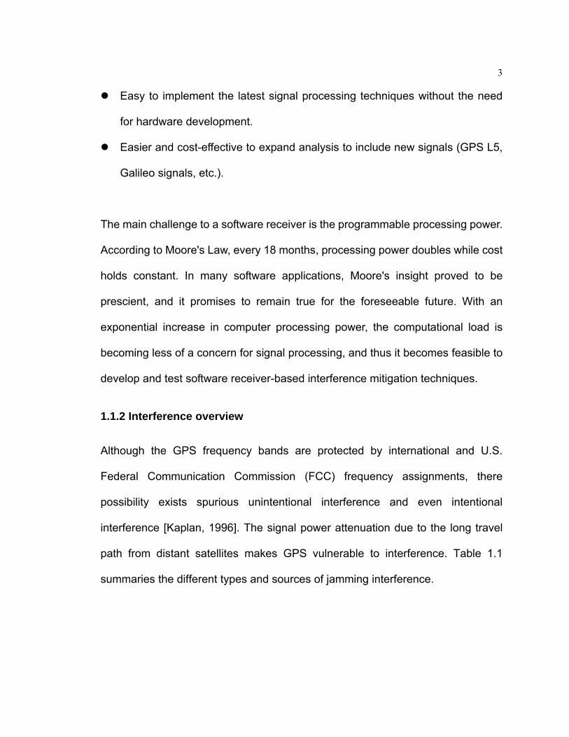
Easy to implement the latest signal processing techniques without the need
for hardware development.
Easier and cost-effective to expand analysis to include new signals (GPS L5,
Galileo signals, etc.).
The main challenge to a software receiver is the programmable processing power.
According to Moore's Law, every 18 months, processing power doubles while cost
holds constant. In many software applications, Moore's insight proved to be
prescient, and it promises to remain true for the foreseeable future. With an
exponential increase in computer processing power, the computational load is
becoming less of a concern for signal processing, and thus it becomes feasible to
develop and test software receiver-based interference mitigation techniques.
1.1.2 Interference overview
Although the GPS frequency bands are protected by international and U.S.
Federal Communication Commission (FCC) frequency assignments, there
possibility exists spurious unintentional interference and even intentional
interference [Kaplan, 1996]. The signal power attenuation due to the long travel
path from distant satellites makes GPS vulnerable to interference. Table 1.1
summaries the different types and sources of jamming interference.

4
Table 1.1: Types and sources of jamming interference
Types of Interference Typical Sources
Wide-band-Gaussian Intentional noise jammers Wide-band phase/frequency modulation
Television transmitter’s harmonics of near-band microwave link transmitters overcoming front-end filter of the GPS receiver
Wide-band-spread spectrum Intentional spread spectrum jammers or near-field of pseudolites
Wide-band-pulse Radar transmissions Narrow-band phase/frequency modulation
AM station transmitter’s harmonics or CB transmitter’s harmonics
Narrow-band-swept continuous wave
Intentional CW jammers or FM stations transmitter’s harmonics
Narrow-band-continuous wave
Intentional CW jammers or near-band unmodulated transmitter’s carriers
[Kaplan, 1996]
The major types of interference can be classified as Additive White Gaussian
Noise (AWGN), narrow-band, and pulsed [Ward, 2002].
AWGN is the best model for thermal noise as well as thermal noise added by
lossy components in the front-end. Broadband interference can also be modeled
as AWGN. The impacts of AWGN on GPS include increasing the noise floor and
reducing the Signal to Noise Ratio (SNR); AWGN also causes cycle slips, jitter in
tracking loops, and bit errors [Ward, 2002]. Narrow-band interference may arise
from spurious signals generated in nearby electrical equipment, or certain types of
jamming. If narrow-band interference is centred close to the carrier frequency (e.g.
L1), it can effectively avoid the selection filter and lead to a Phase Lock Loop (PLL)
5
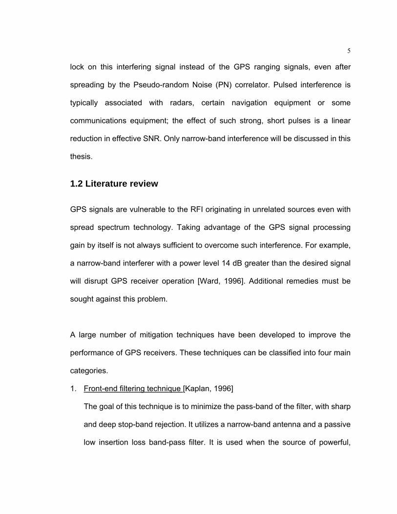
lock on this interfering signal instead of the GPS ranging signals, even after
spreading by the Pseudo-random Noise (PN) correlator. Pulsed interference is
typically associated with radars, certain navigation equipment or some
communications equipment; the effect of such strong, short pulses is a linear
reduction in effective SNR. Only narrow-band interference will be discussed in this
thesis.
1.2 Literature review
GPS signals are vulnerable to the RFI originating in unrelated sources even with
spread spectrum technology. Taking advantage of the GPS signal processing
gain by itself is not always sufficient to overcome such interference. For example,
a narrow-band interferer with a power level 14 dB greater than the desired signal
will disrupt GPS receiver operation [Ward, 1996]. Additional remedies must be
sought against this problem.
A large number of mitigation techniques have been developed to improve the
performance of GPS receivers. These techniques can be classified into four main
categories.
1. Front-end filtering technique [Kaplan, 1996]
The goal of this technique is to minimize the pass-band of the filter, with sharp
and deep stop-band rejection. It utilizes a narrow-band antenna and a passive
low insertion loss band-pass filter. It is used when the source of powerful,
6
near-band interference is known and expected, such as unintentional
interference due to the proximity of a RF source.
2. Code/carrier loop techniques including aiding [Kaplan, 1996]
Jamming performance is improved by narrowing the pre-detection bandwidth
of the receiver as well as the code and carrier tracking loop filter bandwidths.
Reducing these bandwidths also reduces the line-of-sight dynamics that each
channel can tolerate. This can be mitigated somewhat by increasing the loop
filter order for an unaided receiver. But in the presence of accurate external
aiding, it can effectively remove dynamic stress on tracking loops. Examples
of navigation sensors which have been integrated with GPS include Inertial
Measurement Units (IMU), Doppler radar and air speed/baro
altimeter/magnetic compass sensors.
3. Temporal filtering technique [Parkinson and Spilker, 1996]
This technique is effective only for narrow-band jammers. If there is no RFI,
then the thermal noise spectrum will be fairly uniform in the frequency domain.
If there is a significant level of narrow-band interference in the signal it will be
manifested by an anomaly which is above the thermal noise level. The digital
signal processing technique can effectively filter out the narrow-band anomaly
and reduce the narrow-band interference down to the thermal noise level. The
temporal filtering process is accomplished by performing digital signal

7
processing of the digitized IF signal using real time filtering techniques. The
filter can be formed in the time domain using an Adaptive Transversal Filter
(ATF), or in the frequency domain using a Fast Fourier Transform (FFT).
4. Antenna design enhancements [Parkinson and Spilker, 1996]
The main idea of this technique is to increase the antenna gain toward
satellites and decrease gain toward jammers. One type is called a
beam-steered array which points a narrow beam of antenna gain toward each
satellite being tracked. The other type is called a controlled reception pattern
antenna (CRPA), which contains multiple antenna elements physically
arranged into an array that can steer gain nulls toward jammers.
The temporal filtering technique using FFT, combined with an adaptive
code-tracking loop technique will be discussed in detail in this thesis. The
principle of this technique, also referred to as the frequency excision algorithm, is
based on spectrum analysis. If a frequency anomaly is found in the spectrum, this
component will be excised from the corresponding frequency bin [Cutright et al.,
2003].
RFI mitigation using spectrum analysis is not a new technique: much research
has been done, dating back to the early 1980s, e.g. Li and Milstein (1982),
Dipietro (1989), Young and Lehnert (1994), Wang and Amin (1998). These

8
investigations have focused on spread spectrum communications systems. Only
in recent years has such a frequency domain analysis-based interference
mitigation method been applied to GPS by some researchers, namely Peterson et
al. (1996), Badke and Spanias (2002) and Cutright et al. (2003). Most of these
methods were implemented and tested using conventional hardware receivers.
However, many implementation issues, such as the determination of the detection
threshold for different kinds of interference and different interference levels, the
impact of narrow-band interference, the effectiveness of the mitigation algorithm
in a software receiver for signal acquisition and tracking, and position fixing, have
not been fully addressed. Thus, further research into this algorithm, aided by the
flexibility that a software GPS receiver provides could enhance the application of
the frequency excision algorithm in the field of GPS.
1.3 Research objectives
A software GPS receiver developed by the Positioning, Location, and Navigation
(PLAN) research group in University of Calgary provides an excellent platform for
interference study (Ma et al., 2004). Selection of this software receiver platform
provides researchers and developers with more evaluation and testing flexibility
than a comparable hardware platform. New algorithms can be implemented and
receiver parameters can be modified without the cost and delay associated with
hardware development.
The first objective of this thesis is to develop an algorithm to mitigate narrow-band
9
interference that can be embedded into a software Coarse/Acquisition (C/A)-code
GPS receiver to improve anti-jamming performance in terms of accuracy,
reliability and sensitivity.
The second objective is to verify the effectiveness of this algorithm. The
verification will be conducted in a software receiver, and the effectiveness of this
algorithm for signal acquisition, tracking, and position-fixing will be studied. The
maximum tolerance of this algorithm to CW, AM and FM interference and the
effects of the sampling rate on this algorithm will also be investigated.
1.4 Thesis outline
Chapter 1 provides the necessary background information and establishes the
intent and focus of the thesis. Chapter 2 describes the principle of the FFT-based
narrow-band interference mitigation method. Chapter 3 describes the test set up,
the definition of the metrics, and software approaches used in evaluating
mitigation algorithms. Chapter 4 presents the results in the acquisition domain.
Chapter 5 presents the test results in tracking and position domain. Chapter 6
presents the results of kinematic testing. Chapter 7 discusses strategies for
improving the mitigation performance through the use of data windows. Finally,
the conclusions and recommendations for future research are presented in
Chapter 8.

10
CHAPTER 2
Theory of FFT-based Narrow-band Interference Excision and Introduction to
Receiver Technology
The Global Positioning System uses a direct sequence spread spectrum (DS-SS)
signal which incorporates some degree of jamming protection in the signal
structure itself. However, a weak GPS signal - normally in the range of -160 to
-156 dBW for the C/A-code - which is well below the background RF noise level
sensed by an antenna makes it easy for the interference signal to overcome the
inherent jamming protection of the DS-SS signal. Interference signals are spread
in the frequency domain by the GPS signal de-spreading process. These
spectrally dispersed interference signals make it difficult for the GPS receiver to
track the peak of the correlation function. Thus, a frequency-domain interference
excision algorithm is a good approach to mitigate this susceptibility. This algorithm
is, however, effective only against narrow-band interference.
2.1 Narrow-band versus wide-band interference
Narrow-band interference usually occupies more than 100 KHz of bandwidth and

11
less than the entire available spectrum for C/A-code, a bandwidth of 2.046 MHz
[Rash, 1997]. However, qualification of narrow-band signals will also depend on
the bandwidth of the desired signal. For example, a 5 MHz interfering signal can
be regarded as wide if the receiver utilizes a wide correlator design with a 4 MHz
pre-correlation filter; similarly, the same interfering signal can be regarded as
narrow with narrow correlator designs, which have bandwidths of up to 20 MHz.
Unintentional narrow-band interference most often arises from spurious signals
generated by inadequately shielded electrical equipment. Some narrow-band
radio links adjacent to GPS frequencies are also known to cause local
interference problems [MacGougan, 2003].
Wide-band interference occurs across the entire GPS C/A-code spectrum,
covering bandwidths of 2.046 MHz or more. Wide-band interference is also
dependent upon the bandwidth of the original signal. The lower limit of what is
considered wide-band, therefore depends on assignments in the receiver’s
pre-correlation filters. The impact of wide-band interference that is of interest in
this research is the increase in the effective noise floor in a GPS receiver.
Furthermore, when the Jammer-to-Signal ratio (J/S) exceeds the processing gain
of the spreading code, the correlation function is destroyed, making it impossible
to measure the pseudorange.
Wide-band interference in the GPS spectrum originates typically, for example, in
12
television transmitters’ harmonics, or when near-band microwave link transmitters
overcome the front-end filter of the GPS receiver [Kaplan, 1996].
2.2 Fast Fourier Transform
To perform frequency analysis on a discrete-time GPS signal, the time domain
sequence must be converted to an equivalent frequency-domain representation.
Such a frequency-domain representation leads to the Discrete Fourier Transform
(DFT), which is a powerful computational tool for performing frequency analysis of
discrete-time signals.
The Fourier transform separates a waveform or function into sinusoids of different
frequencies which sum to the original waveform. It identifies or distinguishes the
constituent frequency sinusoids and their respective amplitudes.
The Fourier transform of an aperiodic signal with finite duration )t(x is defined as
)F(X :
dte)t(x)F(X Ftπ2j∫= ∞∞−
− (2.1)
The following set of conditions that guarantee the existence of the Fourier
transform are known as the Dirichlet conditions [Proakis, 1996a]:

13
1. the signal )t(x has a finite number of finite discontinuities;
2. the signal )t(x has a finite number of maxima and minima; and
3. the signal )t(x is absolutely integrable; that is,
∞<∫∞∞− dt)t(x (2.2)
In any case, if )t(x is an actual physical component, there always exists a Fourier
transform.
For a finite duration sequence, )n(x of length L, the Fourier transform is as
follows:
π2ω0e)n(x)ω(X1L
0n
nωj ≤≤∑=−
=
− (2.3)
When )(ωX is sampled at equally spaced frequencies
1N,...,2,1,0k,N/kπ2ωk −== where LN ≥ . (2.4)
The resultant samples are
1N,...,2,1,0ke)n(x)k(X1N
0n
N/knπ2j −=∑=−
=
− (2.5)

14
This is a formula for transforming a sequence { )n(x } of length LN ≥ into a
sequence of frequency samples { )k(X } of length N. Since the frequency samples
are obtained by evaluating the Fourier transform )(ωX at a set of N equally
spaced discrete frequencies, )k(X is called the DFT of )n(x .
Direct computation of the DFT is basically inefficient because it does not exploit
the symmetry and periodicity properties of the phase factor, N/π2je−
The FFT is a DFT algorithm developed by Tukey and Cooley (1965) which
reduces the number of computations from something in the order of 2N to
N2logN , by exploiting the symmetry and periodicity properties of the phase factor.
In this algorithm, it re-expresses the DFT of an arbitrary composite size (n = n1n2)
in terms of smaller DFTs of sizes n1 and n2. It first computes n1 transforms of size
n2, and then computes n2 transforms of size n1. The decomposition is applied
recursively to both the n1 and n2 point DFTs. The general Cooley-Tukey
factorization rewrites the indices j and k as j = n2 j1 + j2 and k = n1 k2 + k1,
respectively, where the indices ja and ka run from 0..na-1. That is, it re-indexes the
input (k) and output (j) as n1 by n2 two-dimensional arrays in column-major and
row-major order, respectively. When this reindexing is substituted into the DFT
formula for jk, the n2j1n1k2 cross term vanishes (Its exponential is unity).

15
2.3 Algorithm for FFT-based narrow-band interference mitigation
The interference immunity of a spread spectrum system corrupted by narrow
band interference can be significantly enhanced by excising the interference prior
to correlation of the received signal [Proakis, 1996b]. Several techniques exist for
reducing this interference, including adaptive transversal filters (ATF) [Przyjemski,
et al., 1993], FFTs, and filter banks (FB) [Rifkin and Vaccaro, 2000]. All these
techniques attempt to filter out the interference before correlation. A steady-state
2M+1 tap linear phase ATF utilizes M taps on each side of the centre tap as a 2M
tap linear predictor of the value at the centre tap. This can be expressed in vector
notation as:
nT
Mnn xwxr −= − (2.6)
where w is the length 2M vector of weights and nx is the length 2M vector of
inputs existing at time n.
Therefore, a 2M+1 tap linear phase filter is realized with M complex multipliers, M
complex adders, and an M+1 complex adder tree utilizing )1M(2log + complex
adders. The computational complexity of this ATF based method determines if it
can be implemented in ASIC, but is not efficient in a software receiver. The
number of computations for FFT based methods is N2logN . This method is used
in this thesis, because it has the potential to be implemented in a real time
software receiver. Filter bank represents an extension of the FFT based method

16
that attempts to further reduce the signal loss by extending the effective FFT
length. The FB allows the spectrum estimation to occur more or less frequently
and the filtering is performed over an arbitrary length. The testing of this method is
left for future research.
The objective of the FFT-based narrow-band interference algorithm is to reduce
the level of the interference; this is achieved at the expense of introducing some
degree of distortion on the desired signal. The estimation and suppression of
interference can be performed in the frequency domain by using DFT, which is
efficiently implemented via an FFT algorithm. The received base band signal is
processed in fixed-length blocks, transformed to the frequency domain with an
FFT, filtered by using an appropriate weighting, and then transformed back into
the time domain.
The received base band data stream has three components; namely, the signal
samples ks , the broadband noise samples kη , and the narrow-band interference
sample kθ . Each component is assumed to be uncorrelated with the other two and
characterized by a zero mean. The individual component correlations [Dipietro,
1989] are given as:
[ ]⎩⎨⎧
=≠
=mkSmk0
ssE *mk (2.7)
17
[ ]⎪⎩
⎪⎨⎧
=
≠=
mkσ
mk0ηηE 2
*mk (2.8)
km*mk r]θθ[E −= (2.9)
where [ ]E is the expectation operator and * denotes a complex conjugate.
Hence, the signal and noise samples are each uncorrelated, while the
narrow-band interferences are correlated.
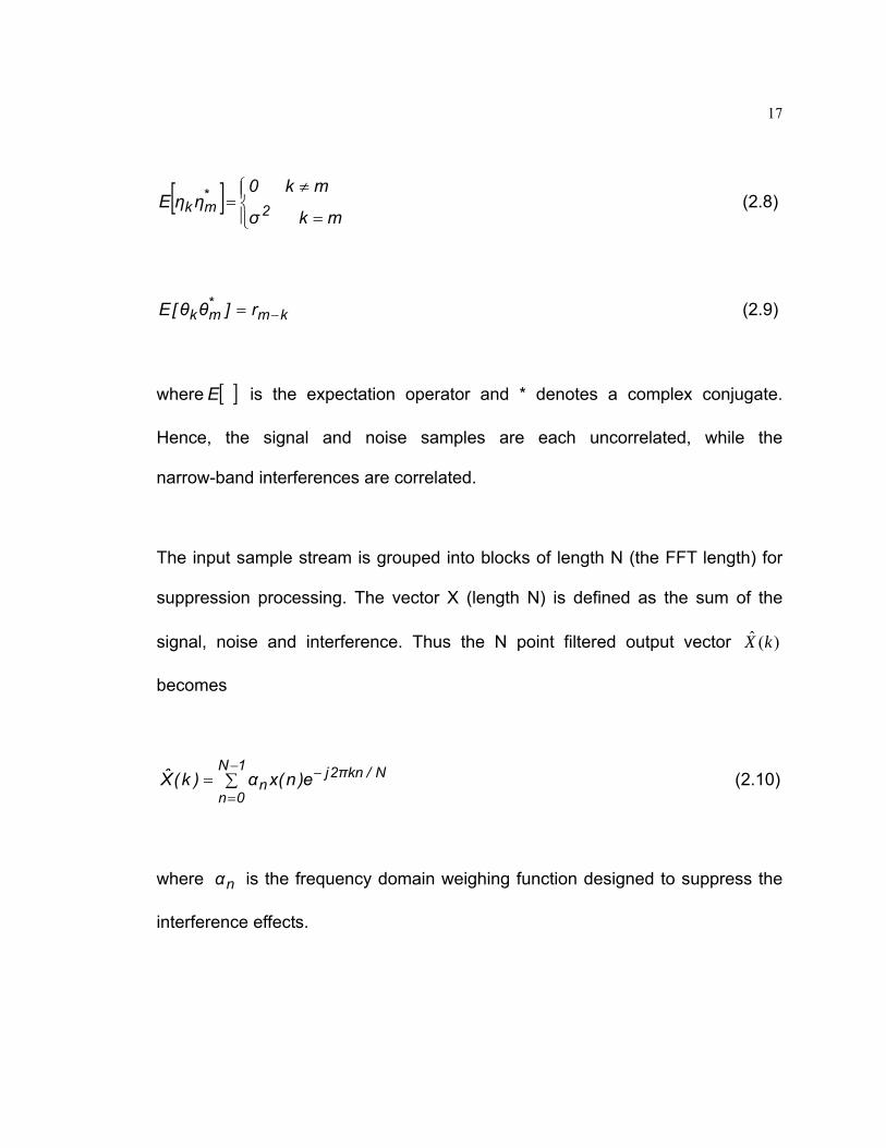
The input sample stream is grouped into blocks of length N (the FFT length) for
suppression processing. The vector X (length N) is defined as the sum of the
signal, noise and interference. Thus the N point filtered output vector )(ˆ kX
becomes
∑=−
=
−1N
0n
N/knπ2jn e)n(xα)k(X (2.10)
where nα is the frequency domain weighing function designed to suppress the
interference effects.

18
The SNR at the output of the correlator is given by:
)Xs(Var
])Xs[E(SNR H
k
2Hk= [Dipietro, 1989] (2.11)
where Var () is the variance operator and H denotes the conjugate transpose.
If the corresponding component in Equation 2.10 is replaced by the assumed
statistical properties of the signal components and the characteristics of the DFT
transformation matrix, this yields the SNR in the form:
3d2d1dS)α(
SNRN
1k2
k++
∑= = (2.12)
with
( )⎟⎟
⎠
⎞
⎜⎜
⎝
⎛ ∑−∑= =
= Nα
αS1dN
1k2kN
1k2k (2.13)
where 1d is a “self noise” term which is analogous to that seen in linear
prediction suppression processors [Proakis and Ketchum, 1982] - a term that
vanishes in the case of no filtering.
∑= =N
1k2k
2 ασ2d (2.14)
where 2d is the residual broadband noise.

19
∑= =N
1k2
kk )α(N13d Θ (2.15)
where 3d is narrow-band interference power, and
kΘ is the kth FFT bin component of the narrow-band interference signal.
If the value of kα is set at unity, this yields an expression of the
pre-suppression SNR as:
∑+=
=N
1k2
k2 )θ(
N1σ
NSSNR [Dipietro, 1989] (2.16)
where N is the FFT length for suppression processing and S is equal to
]ss[E *kk .
Comparing the two equations, 2.11 and 2.15, the ratio of these two equations
yields the improvement factor used to assess interference mitigation
performance.
A thresholding algorithm is used to determine the weighting function. From either
the model or real world data, the distribution of interferer powers suggests that
only a small number of frequency domain cells contain nearly all of the
interference power within the band [Dipietro, 1989]. Based on this conclusion, one
possible strategy would be to set the weights on all cells with large interference
values to zero, while leaving the others at unity. The computational challenge lies
20
in determining which cell constitutes a large interference. One way is to establish
a threshold and any cell magnitude exceeding this level is declared as
interference and removed by setting its corresponding weighting function to zero.
The threshold may be established on the basis of knowledge of the interference
distribution, or on the basis of heuristic experience, such as setting the threshold
to excise a fixed percentage of the cells or total interference power. The other
strategy would be to set any cell value exceeding the threshold to the background
noise level, and thus whiten the interference spectrum. This approach will yield
improved results, because the cell value containing interference will be reduced
only to the background level, hence retaining most of the signal power. The
drawback to this approach, however, is the requirement for the background noise
level to be estimated, producing the unwanted consequence of increasing the
computational burden.
2.4 Introduction to GPS receiver technology
The FFT-based interference mitigation algorithm is developed in a software GPS
receiver in this thesis. The impact of different receiver design parameters on the
mitigation results will also be discussed. An overview to GPS receiver technology
and criterion for choosing design parameters will be provided in this section.
2.4.1 GPS signal acquisition overview
GPS signal acquisition is a two-dimensional search process, as illustrated in

21
Figure 2.1 below [Lin and Tsui, 2000]. The range dimension is associated with the
replica code, while the Doppler dimension is associated with the replica carrier.
Figure 2.1: GPS signal acquisition
Pre-determination of the code phase is difficult because this is a function of the
starting point and is dependent on the sampling rate. The code search space
typically includes all possible code offset values. All 1023 C/A-code phases must
therefore be searched. The combination of one code bin and one Doppler bin
constitutes a searching cell. The Doppler change is a function of user dynamics
and the stability of the receiver oscillator. If the Doppler uncertainty is unknown,
the maximum user velocity plus maximum SV Doppler must be searched in both
directions about zero Doppler. The Doppler searching space is usually from -5
kHz to 5 kHz [Ray, 2003]. The frequency resolution is determined by the coherent

22
integration time, which is also referred to as the dwell time. The rule-of-thumb
Doppler bin is defined as follows to avoid significant signal attenuation due to
frequency errors [Ward, 1996]:
)T3/(2f =∆ (2.17)
where T represents the coherent integration time.
The coherent integration time restricts the size of Doppler bins used in acquisition
mode. Dwell times can vary from less than 1.0 ms for strong signals up to 20.0 ms
for weak signals. It can be seen from Equation 2.16 that the corresponding
Doppler bins are 667 Hz and 33 Hz. The poorer the expected C/N0 ratio, the
longer the dwell time (and overall search time) must be in order to have
reasonable success in signal acquisition [Kaplan, 1996]. Longer integration can
provide improved frequency resolution and higher sensitivity, but this entails
searching a larger number of bins and requires more time. Thus, there is a
trade-off between the pre-detection integration time and acquisition speed.
Various acquisition methods incorporating search and detect strategies have
been proposed in the literature [Krumvieda et al., 2001; Kaplan, 1996]. A
cell-by-cell search method is usually used in conventional hardware receivers. In
this method, the search region is divided into a number of cells of equal size. A
local carrier is generated corresponding to a frequency bin and beat with the
23
incoming signal. A local code stream, corresponding to a code chip delay, is
generated and then correlated with the incoming signal. The local code is shifted
to correlate with the incoming signal until the peak is detected or all the cells are
exhausted. The acquisition time is, therefore, the product of the dwell time and the
number of search bins. Consequently, the acquisition time is very long, since the
search is sequential in nature.
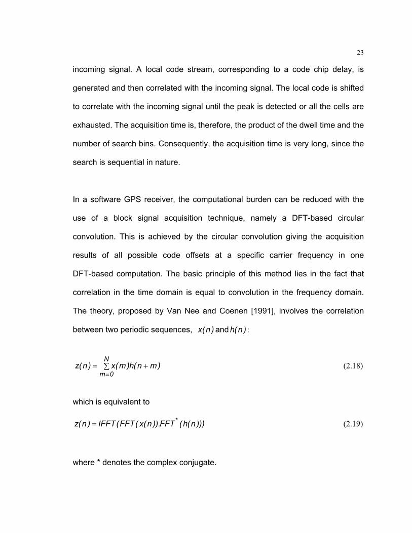
In a software GPS receiver, the computational burden can be reduced with the
use of a block signal acquisition technique, namely a DFT-based circular
convolution. This is achieved by the circular convolution giving the acquisition
results of all possible code offsets at a specific carrier frequency in one
DFT-based computation. The basic principle of this method lies in the fact that
correlation in the time domain is equal to convolution in the frequency domain.
The theory, proposed by Van Nee and Coenen [1991], involves the correlation
between two periodic sequences, )n(x and )n(h :
∑ +==
N
0m)mn(h)m(x)n(z (2.18)
which is equivalent to
)))n(h(FFT)).n(x(FFT(IFFT)n(z *= (2.19)
where * denotes the complex conjugate.

24
The correlation value at all possible code offsets can be calculated in one DFT
operation which greatly reduces the computational burden. Even faster
acquisition speed can be achieved if FFT is applied. This is the basis for choosing
the FFT-based acquisition algorithm for investigation in this thesis.
2.4.2 GPS signal tracking overview
Acquisition produces a coarse estimate of the carrier Doppler and the code offset
of incoming signals. The function of tracking is to track variations in the carrier
Doppler and code offset due to line-of-sight dynamics between satellites and the
receiver, together with bit and sub-frame synchronization to demodulate the
navigation data to obtain ephemeris data. Figure 2.2 below illustrates the block
diagram of the GPS receiver tracking loop.

25
Figure 2.2: GPS receiver signal tracking loop
Both the carrier lock loop (frequency lock loop (FLL) or phase lock loop (PLL)) and
delay lock loop (DLL) are required for signal tracking to match the carrier phase
and code offset with the locally generated carrier and code. The carrier
pre-detection integrators, the carrier loop discriminators and the carrier loop filters
characterize the receiver carrier tracking loop. However, a paradox becomes
apparent during determination of these three parameters. To maximize tolerance
to dynamic stress, the pre-detection integration time should be short, the
discriminator should be a FLL, and the carrier loop filter bandwidth should be wide.
However, if interference exists or under weak signal conditions, the pre-detection
integration time should be long and the carrier loop filter noise bandwidth should
be narrow [Kaplan, 1996]. In order to obtain more accurate carrier Doppler phase
LP
NCO Code Gene
Code Loop Filter
Phase Loop Filter
NCO
cos
S
sin
P
E-L
I
Q
IE-L
QE-L
IP
QP
f,φ
τ
Fτ
FF f,φ
LP
LP
LP
Code and Phase Discriminators
Lock Detector & C/N0 Estimation
Lock status
Data bit

26
measurements, the discriminator should be PLL instead of FLL. In implementation,
some compromises have to be made. The tracking loop will start with a short
pre-detection integration time, using a FLL and a wide-band carrier loop filter.
Then it switches to a Costas PLL with its pre-detection bandwidth and carrier
tracking loop bandwidth set as narrow as the dynamics permit. It will revert to FLL
operation during periods of high dynamic stress if necessary.
A DLL is used to track the C/A-code phase of incident signals. As in a regular
phase lock loop, it consists of a code phase discriminator, a loop filter, and the
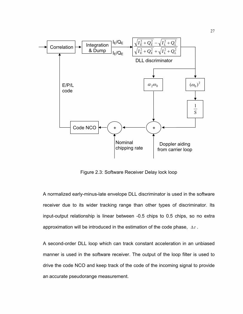
C/A-code numerically-controlled oscillator (NCO). Figure 2.3 illustrates a typical
DLL realized in the software receiver with a second order phase lock loop which
tolerates constant acceleration [Ward, 1996 and Dong, 2003].
27
Figure 2.3: Software Receiver Delay lock loop
A normalized early-minus-late envelope DLL discriminator is used in the software
receiver due to its wider tracking range than other types of discriminator. Its
input-output relationship is linear between -0.5 chips to 0.5 chips, so no extra
approximation will be introduced in the estimation of the code phase, τ∆ .
A second-order DLL loop which can track constant acceleration in an unbiased
manner is used in the software receiver. The output of the loop filter is used to
drive the code NCO and keep track of the code of the incoming signal to provide
an accurate pseudorange measurement.
Correlation Integration & Dump
IE/QE
IE/QE
2222
2222
LLEE
LLEE
QIQI
QIQI
+++
+−+
DLL discriminator
Code NCO
Nominal chipping rate
Doppler aiding from carrier loop
E/P/L code
+ +
02ωα 20 )(ω
S1
28
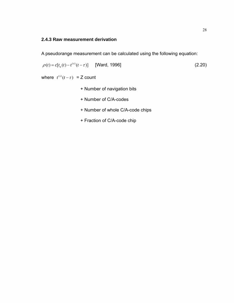
2.4.3 Raw measurement derivation
A pseudorange measurement can be calculated using the following equation:
)]()([)( )( τρ −−= ttttct su [Ward, 1996] (2.20)
where )()( τ−tt s = Z count
+ Number of navigation bits
+ Number of C/A-codes
+ Number of whole C/A-code chips
+ Fraction of C/A-code chip
29
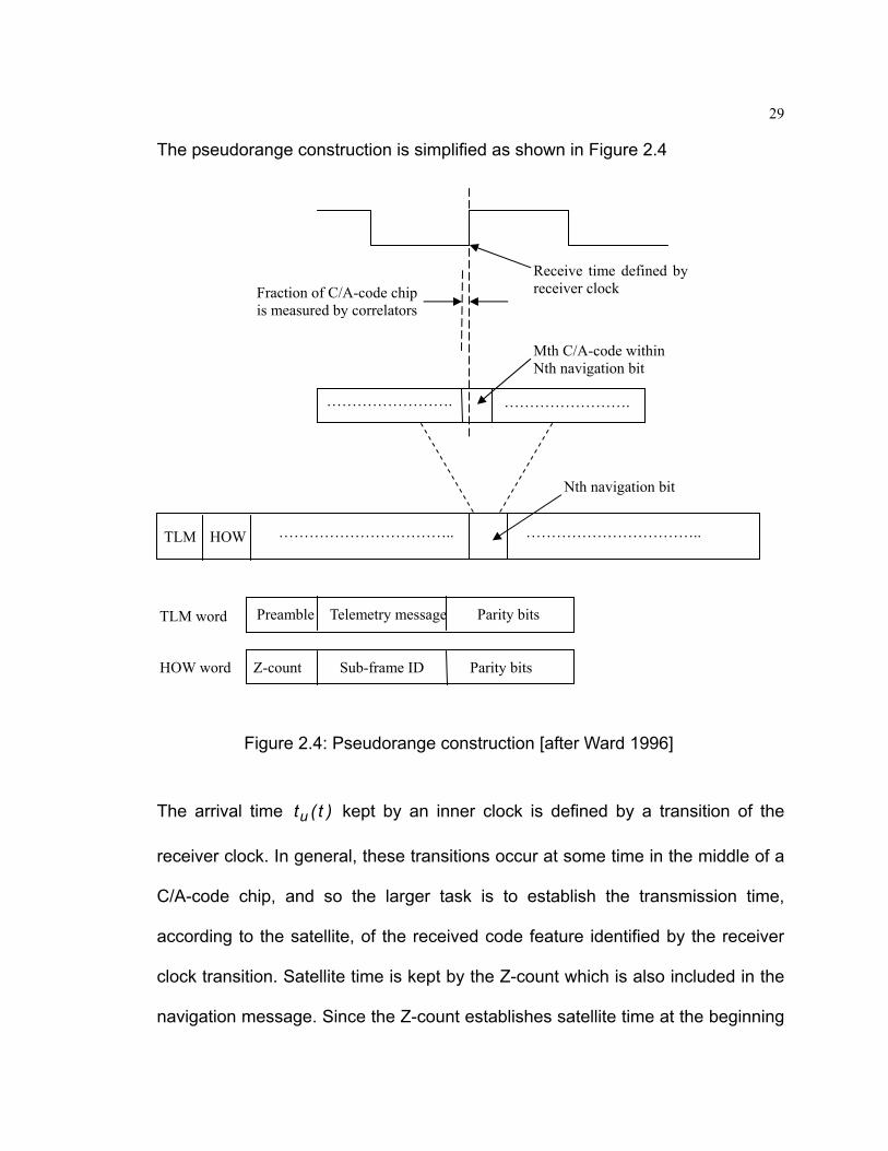
The pseudorange construction is simplified as shown in Figure 2.4
Figure 2.4: Pseudorange construction [after Ward 1996]
The arrival time )t(tu kept by an inner clock is defined by a transition of the
receiver clock. In general, these transitions occur at some time in the middle of a
C/A-code chip, and so the larger task is to establish the transmission time,
according to the satellite, of the received code feature identified by the receiver
clock transition. Satellite time is kept by the Z-count which is also included in the
navigation message. Since the Z-count establishes satellite time at the beginning
TLM HOW …………………………….. ……………………………..
Nth navigation bit
……………………. …………………….
Mth C/A-code within Nth navigation bit
Fraction of C/A-code chipis measured by correlators
Receive time defined by receiver clock
TLM word Preamble Telemetry message Parity bits
HOW word Z-count Sub-frame ID Parity bits

30
of each sub-frame, the transmission time is the Z-count plus the whole number of
C/A-code chips since the beginning of the sub-frame. The elapsed time can be
measured using the following components: the whole number of navigation bits,
added to the whole number of C/A-codes since the beginning of the current
navigation bits, added to the number of whole C/A-code chips since the beginning
of the current code and added to the received fraction of the current chip. The last
two are measured by the DLL and the rest are measured by counters in the bit
synchronization and sub-frame synchronization modules.
The Doppler measure can be read directly from the carrier NCO while the carrier
phase must be assisted by a carrier counter which is used to count the integer
number of cycles that the incoming carrier has changed. The fractional portion is
recorded with the carrier NCO; the summation of the integer and fractional parts
gives the carrier phase measurement since locking of the loop.
After the pseudorange and carrier phase raw measurements have been derived,
a least squares approach is employed to estimate the position solution and clock
bias.
2.4.4 Loop filter determination
The objective of the loop filter is to reduce noise in order to produce an accurate
estimate of the original signal at its output. The loop filter order and noise
bandwidth determine the loop filter’s response to signal dynamics. The loop filter’s

31
output signal is effectively subtracted from the original signal to produce an error
signal, which is fed back into the filter’s input in a closed loop process.
The type of tracking loop chosen depends on the following design factors:
Desired tracking performance
Desired noise bandwidth (and resulting SNR), and
Anticipated user dynamics
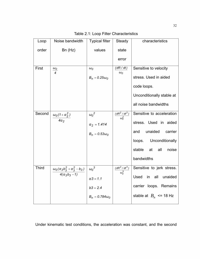
Table 2.1 summarizes the typical values and characteristics of first order, second
order and third order tracking loops [Kaplan, 1996].
32
Table 2.1: Loop Filter Characteristics
Loop
order
Noise bandwidth
Bn (Hz)
Typical filter
values
Steady
state
error
characteristics
First 4ω0 0ω
0n ω25.0B = 0ω
)dt/dR(
Sensitive to velocity
stress. Used in aided
code loops.
Unconditionally stable at
all noise bandwidths
Second
2
220
α4)α1(ω +
20ω
414.1α2 =
0n ω53.0B =
20
22
ω)dt/dR( Sensitive to acceleration
stress. Used in aided
and unaided carrier
loops. Unconditionally
stable at all noise
bandwidths
Third )1bα(4
)bαbα(ω
33
323
2330
−
−+ 30ω
1.13α =
4.23b =
0n ω784.0B =
30
33
ω)dt/dR( Sensitive to jerk stress.
Used in all unaided
carrier loops. Remains
stable at nB <= 18 Hz
Under kinematic test conditions, the acceleration was constant, and the second

33
order loop filter is sensitive enough to detect the acceleration stress. The second
order loop filter is unconditionally stable at all noise bandwidths. By comparison,
the third order loop filter is stable only when nB <= 18 Hz [Kaplan, 1996], and the
computational burden is high. The combination of robustness under kinematic
stress and a manageable computational load support the choice of the second
order loop filter for test purposes.
The block diagram of a second order loop filter is shown below [Kaplan, 1996]:
Figure 2.5: Second order loop filter
In Figure 2.5, analog integrators are represented by 1/s, the Laplace transform of
the time domain integration function. This transform can be implemented in digital
form as shown in Figure 2.6.
ω02
a2ω0
∑ S1
S1

34
Figure 2.6: Digital representation of Laplace transform
The input )(nx which is quantized to a finite resolution produces a discrete
integrated output, )n(Y as )1n(A)]n(x[T)n(y −+= , where n is the discrete
sample sequence number.
The time interval between each sample T represents a unit delay in the
digital integrator. This provides a dynamic range capability. A comparatively long
integration time produces a long response time and hence is not suitable for high
dynamic conditions. If the signal is weak, for example, and interference occurs, a
longer integration time is required. A balance must be made to achieve optimal
sensitivity and accuracy.
T ∑+
+
A
)n(Y
1Z−
)n(x
1Z −
35
CHAPTER 3
Test Setup and Methodology
In order to obtain repeatable and controllable GPS signals with narrow-band
interference, a hardware GPS simulator and signal generator were used. These
two signals were combined in an interference combiner unit. The output was fed
to a Signal Tap which down-converts RF signals to IF signals and samples them.
The resulting data was used in the software receiver and a mitigation algorithm
was used to assess the acquisition, tracking and position performance. This
chapter addresses the test setups and software approaches of the mitigation
algorithms studied.
3.1 RF GPS signal with interference generation
3.1.1 GSS STR6560 multi-channel GPS/SBAS simulator
The PLAN group of the University of Calgary possesses two synchronous
12-channel L1-only hardware signal simulation units (GSS STR 6560) associated
to a control computer made by Spirent Communications Inc. which is capable of
providing comprehensive facilities for development and product testing of satellite
navigation equipment and integration studies. The simulator can also reproduce

36
the environment of a navigation receiver installed on a dynamic platform,
exhibiting the effects of high-dynamic host vehicle motion, navigation satellite
motion and ionospheric and tropospheric effects. The simulator may be
considered as a pseudorange-to-RF converter. Each channel represents a
satellite signal at a single carrier frequency. The simulator’s capabilities include
the following [Spirent, 2003a]:
Control of the signal power for each channel
Complex simulated vehicle trajectories
Multipath simulation
Satellite constellation definition and modeling
Atmospheric effects modeling (Ionosphere/Troposphere)
Vehicle motion modeling for aircraft, cars, and spacecraft
User-supplied motion trajectories
Antenna gain pattern manipulation
Pseudorange error ramping
Terrain obscuration modeling
ASCII format scenario files (sharable between scenarios)
Real time data display, and
Post-mission truth data output
3.1.2 Interference generation combined with GPS signal
The narrow-band interference simulated in the test (continuous wave (CW),

37
amplitude modulation (AM) and frequency modulation (FM)) was generated by an
ESG E4431B signal generator. It can provide a maximum specified frequency of 2
GHz, at a maximum specified power of 10 dBm which is sufficient to jam GPS
signals. The GPS and interference signals were combined in a GSS 4766
interference combiner unit which facilitates the use of commercial-off-the-shelf
(COTS) signal generators as fully integrated interference sources with Spirent
Satellite Navigation Simulators, such as the GSS 6560. The COTS signal
generators are controlled through an IEEE-488-compliant (GPIB) bus, via
SimGEN for Windows, hosted on the control PC. The interference signal is
defined along with all the other scenario parameters from within SimGEN’s normal
user GUI environment. The RF outputs are combined with the satellite signal
generators (SSG) in the GSS 4766 interference combiner unit (ICU). The system
hardware configurations are shown in Figure 3.1.

38
Figure 3.1: System hardware configuration

39
3.2 Intermediate frequency signal generation, sampling and
quantization
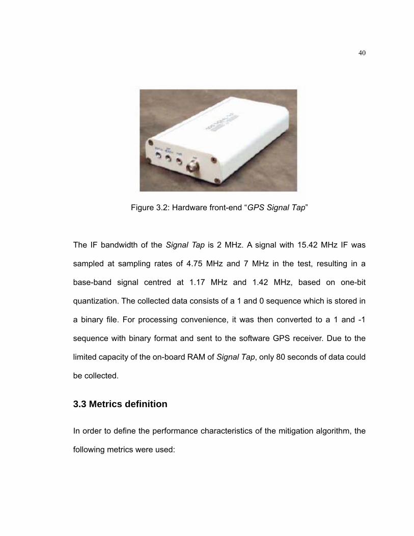
A hardware front-end, GPS Signal Tap (Figure 3.2), made by Accord Software &
Systems Private Limited was used to collect the digitized IF signal. Only after
down-converting, sampling and quantizing can the GPS data be processed by the
software receiver. Accord’s GPS Signal Tap is an L1 frequency GPS receiver
front end, which serves as a programmable real time source of digitized GPS
signals for a variety of desktop research and development tasks related to signal
processing. The Signal Tap consists of a two-stage RF down-converter whose
second IF can be sampled and stored for analysis by the user at a programmable
frequency [Accord, 2003]. The RF down-converter obtains the input GPS satellite
signal from an antenna-cable assembly. It uses mixers, local oscillators and band
pass filters to down-convert the carrier to a low IF. The IF is then sampled by a
chosen sampling frequency to generate the digitized IF signal of the satellites.
40
Figure 3.2: Hardware front-end “GPS Signal Tap”
The IF bandwidth of the Signal Tap is 2 MHz. A signal with 15.42 MHz IF was
sampled at sampling rates of 4.75 MHz and 7 MHz in the test, resulting in a
base-band signal centred at 1.17 MHz and 1.42 MHz, based on one-bit
quantization. The collected data consists of a 1 and 0 sequence which is stored in
a binary file. For processing convenience, it was then converted to a 1 and -1
sequence with binary format and sent to the software GPS receiver. Due to the
limited capacity of the on-board RAM of Signal Tap, only 80 seconds of data could
be collected.
3.3 Metrics definition
In order to define the performance characteristics of the mitigation algorithm, the
following metrics were used:

41
(1) C/N0: Carrier-to-Noise Density Ratio (dB). It is one of the most important
measurement values used to define the quality of a signal. The nominal noise
floor has a spectral density of approximately -204 dBW/Hz. The minimum
guaranteed GPS signal power for L1 C/A-code is -160 dBW, which implies a C/N0
equal to C – N0 = 44 dBW-Hz. Receivers incorporating different correlation
processes will have differences in C/N0; the short term variation in the C/N0 can
be used as an estimate of signal degradation caused by interference.
(2) Jamming-to-Signal ratio (J/S). J/S = J-S (dB), where S and J are the incident
signal power and incident jamming power, respectively, at the antenna. This
measure, which can be controlled through SimGEN software, characterizes the
relative interference power compared with the GPS signal strength.
(3) Estimated pseudorange errors: these errors are calculated by using
C3NavG2TM, a software package developed by University of Calgary’s PLAN
Group. C3NavG2TM is a C-language program that processes pseudoranges and
Doppler data in both static and kinematic modes to determine position and
velocity in either single point or differential mode. An epoch-by-epoch
least-squares solution is used, which is highly suitable for the type of sensitivity
analysis required herein. This software allows the measurement of the
degradation due to the interference on the pseudorange measurements.

42
(4) Position domain: With knowledge of the true position and velocity of the
receiver from the output of the simulator, position and velocity errors can be
computed. Hence, navigation performance in the presence of interference
mitigation effects can be investigated.
Errors due to multipath and atmospheric effects have been removed from all of
the tests in this thesis in order to isolate the errors of interest. Only interference
and random noise will have an influence on the results.
In order to keep exactly the same conditions for all tests, all simulations were
processed within the same period and satellite constellation: November 17, 2003,
from 13:30:26 to 13:31:46. Only the sky view at the beginning of the simulation
was provided in Figures 3.3, because the constellation changes very little in 80
seconds.

43
Figure 3.3: Sky view at the beginning of the simulation
3.4 Software approach of FFT-based mitigation algorithm
Prior to de-spreading, the GPS signal has noise-like characteristics over the
system bandwidth. Therefore, any narrow-band RFI has strong correlations
between samples in which the GPS signals are uncorrelated. Therefore, the
spectral peaks of interference can be discriminated and suppressed from the GPS
signal and the thermal noise (Gaussian distribution) through an adaptive
threshold power level and an adaptive notch filter.

44
3.4.1 Interference detection
The first stage of an FFT-based interference mitigation algorithm is interference
detection. Three methods are normally used for independent on-board
interference monitoring:
1) Correlator power Output
The correlator power output indicates the average post-correlation SNR which is
computed from the following equation:
Floor_Noise_ExpectedQISNR
22pc
+= (3.1)
where I and Q are the 1 ms In-phase and Quadra-phase prompt correlator signals,
respectively. The level and variance of pcSNR are a function of noise and
interference in the signal, and therefore are candidates for interference detection.
2) Carrier Phase Vacillation
Carrier phase vacillation provides a measure of the variance or jitters in carrier
phase measurements from one measurement epoch to the next, and is defined as
[Ndili and Enge, 1997]:
TCPCP
CPV 1ii −−= (3.2)

45
where CPV = Carrier phase Vacillation
CP = Carrier phase
T = Time duration of epoch
i = Epoch index
T is the time duration of epoch and i is the epoch index
The carrier phase referenced above is computed from the arctangent of the
In-phase and Quadra-phase measurements. Phase swings of 180 degrees, due
to data bit changes, are taken into account and do not affect the detection results.
Receiver clock noise as well as interference contributes to vacillations in the
carrier phase measurements. Interference contributes most, so carrier phase
vacillation is therefore a candidate for interference detection. The limitation of this
method is that it is only effective for a medium level interference. When the
interference level is high, no carrier phase can be tracked, thus carrier phase
vacillation cannot be calculated.
3) Automatic gain control (AGC) gains
The control loop of the AGC, located on the signal down-conversion/digitization
path, acts by adjusting the threshold levels of the adaptive analog-to-digital
converter (ADC) to maintain a specified ratio of digitized signal output levels. The
quantizer threshold level is therefore associated with the interference level and
can be used as an indication of the occurrence of interference.

46
Table 3.1 shows the summarized decision statistic results with CW interference,
with percentages of incidence of false alarm (FA), missed detection (MD), normal
operation (NO) and normal detection (ND) [Ndili and Enge, 1997]. Normal
operation means the decision statistic result falls in the region of correct detection,
while normal detection means the result falls in the region of correct non-detection
as shown in Figure 4.5.
Table 3.1: Decision statistic results summary
MD FA NO ND
Correlator
Power output
0.0% 3.0% 56.7% 40.3%
Carrier Phase
Vacillation
0.0% 10.4% 49.3% 40.3%
AGC Gain 0.0% 1.5% 58.2% 40.3%
Because the control of the AGC in the Signal Tap cannot be accessed, the AGC
gain method was not taken into account. Due to the relative large false alarm rate
of the carrier phase vacillation method, the correlator power output method was
viewed as a better method for use in this thesis.
3.4.2 Interference mitigation
The basic principle of an FFT-based mitigation algorithm is to determine the
statistical properties of non-Gaussian distributed interference and to improve the

47
SNR by eliminating all interference. The mitigation process will certainly cause
signal loss. So, if the interference has been successfully detected, the mitigation
algorithm is applied to the input data; if, not, the normal acquisition and tracking
procedure is applied directly.
This algorithm first transforms the incoming IF signal into the frequency domain
using the FFT. In order to remove the bias in the frequency domain due to the
bandwidth and the non-linear property of the Signal Tap, the signal is averaged
over small intervals and the resulting mean is subtracted from the spectrum over
the corresponding interval.
Figures 3.4 and 3.5 compare the 1 ms FFT results with and without CW
interference (no unit for power spectrum).

48
0 1000 2000 3000 4000 5000 6000 70000
500
1000
1500
2000
2500
3000
Sample number
Squ
are
root
of p
ower
spe
ctru
m
Figure 3.4: 1 ms FFT without CW interference
0 1000 2000 3000 4000 5000 6000 70000
500
1000
1500
2000
2500
3000
Sample number
Squ
are
root
of p
ower
spe
ctru
m
Figure 3.5: 1 ms FFT with CW interference (J/S = 30 dB)

49
The 1 ms FFT analysis period is from –π to πand, so, the spectrum is
symmetrical. The natural frequency ω0 lies in the middle of the sample number
axis (X axis). It can be seen from Figure 3.6 that, even with one pure tone CW
interference, the influence of CW interference in the frequency domain is not a
single line. Interference spreads out through the whole spectrum due to the finite
FFT analysis period which causes spectral leakage (a detailed analysis of the
mitigation of spectral leakage effects will be given in Chapter 7). So simply
removing one frequency component with the largest power spectrum line is not
sufficient. In implementation, further analysis is needed to decide which frequency
component must be removed. The judging criterion is based on the statistical
analysis of the input signal. Traditionally, the standard deviation of the resulting
normalized spectrum is multiplied by a fixed value to set a detection threshold for
determining the presence of RFI [Cutright et al., 2003]. The optimal estimate of
this fixed value is determined empirically. However, for high-level interference, a
fixed detection threshold is not good enough. Since the post-correlation SNR is a
good indicator of interference level, it is reasonable to associate the detection
threshold with the post-correlation SNR. In this thesis, an adaptive interference
detection threshold determination method that is a function of the standard
deviation of the normalized spectrum and the post-correlation SNR is used. The
test results show that better performance can be achieved through this adaptive
detection threshold. After the detection threshold is determined, the normalized
spectrum is then compared against the threshold and bins exceeding the

50
detection level are identified. The bins containing RFI, along with a variable
number of surrounding bins, are then set to zero in the original frequency domain
spectrum. The effect of removing the frequency bins is equal to applying
band-pass filters in the time domain. The Inverse Fast Fourier Transform (IFFT) of
this spectrum is taken which yields a new time domain signal without RFI.
Figure 3.6 shows the flowchart of the frequency excision algorithm. In summary,
in order to obtain the optimal anti-jamming performance, three parameters have to
be carefully chosen:
1) the average interval to remove bias
2) detection threshold, and
3) the number of samples to be removed near the bin containing the RFI

51
Figure 3.6: Flowchart of frequency excision algorithm
Remove the average values
Normal acquisition and tracking
Set identify threshold
Set corresponding spectrum to zero
Judge which component is above
the threshold
IFFT
FFT
Average
Take absolute value of FFT
Get standard deviation
Y
N
+
-
IF input RFI
Present?

52
CHAPTER 4
Mitigation Analysis in Acquisition
4.1 CW Interference frequency determination
The GPS C/A-code is a Gold code with a short 1 ms period. Because of this, the
C/A-code does not have a continuous power spectrum. Instead, it has a line
spectrum whose components are separated by 1 KHz [Ward, 1996]. Figure 4.1
illustrates a typical Gold code spectrum from the GPS constellation.
Figure 4.1: Spectrum of Gold code [from Heppe, 2002]

53
While the envelope of the spectrum approximates an ideal Sinc function, a clear
line spectrum can be observed, with some components above and some below
the ideal envelope. A narrow-band RFI signal could accidentally coincide with a
strong spectral line of the Gold code and leak through the correlator, leading to a
stronger than expected residual line into the PLL. Thus, narrow-band interference
can be potentially more damaging than expected due to the line spectrum of the
Gold codes used for ranging.
Although it is typical for each line in the C/A-code power spectrum to be 24 dB or
more lower than the total power [Ward, 1996], there are usually some lines in
every C/A-code that are stronger. These phenomena cause more of a problem
during C/A-code acquisition than in tracking. Table 4.1 summarizes the worst line
frequencies and the worst line (strongest) amplitudes for every Pseudorandom
Noise (PRN) code used in GPS [Ward, 1996].

54
Table 4.1: Worst C/A line for each of the 37 codes
C/A-code PRN
Number
Worst line Frequency
(kHz)
Worst Line Amplitude
(dB)
C/A-code PRN
Number
Worst line Frequency
(kHz)
Worst Line Amplitude
(dB)
1 42 -22.71 20 30 -22.78 2 263 -23.12 21 55 -23.51 3 108 -22.04 22 12 -22.12 4 122 -22.98 23 127 -23.08 5 23 -21.53 24 123 -21.26 6 227 -21.29 25 151 -23.78 7 78 -23.27 26 102 -23.06 8 66 -21.50 27 132 -21.68 9 173 -22.09 28 203 -21.73 10 16 -22.45 29 176 -22.22 11 123 -22.64 30 63 -22.14 12 199 -22.08 31 72 -23.13 13 214 -23.52 32 74 -23.58 14 120 -22.01 33 82 -21.82 15 69 -21.90 34 55 -24.13 16 154 -22.58 35 43 -21.71 17 138 -22.50 36 23 -22.23 18 183 -21.40 37 55 -24.13 19 211 -21.77
In this thesis, the CW interference frequency was set at 1575.462 MHz, offset by
42 KHz from the central frequency of L1. From Table 4.1, it is clear that this is the
worst line frequency of PRN 1. This interference frequency is chosen to obtain the
strongest interference for PRN 1. The following analysis in acquisition and

55
tracking is based on PRN 1. Thus, the mitigation performance achieved is under
the worst conditions for this code.
4.2 Impact of CW interference on correlation function
4.2.1 CW frequency effect on correlation function
In this test, the C/A-code signal was mixed with CW interference with a power
level of 10 dB higher than the code signal and a frequency that varied from the
central frequency of L1 by 2.8 kHz to 500 kHz. Figure 4.2 depicts the correlation
result, where the delta frequency is the code spectral line on which the CW
interference is superimposed.
Figure 4.2: Correlations for different spectral lines
It can be seen that both the correlation functions have actually a sinusoidal
function whose oscillation frequency depends on the CW interference frequency.
So interference occurring at different frequencies will have totally different effects

56
on GPS signal acquisition or tracking. For ∆f = 42 kHz, the generated correlation
is worse because the autocorrelation peak is difficult to identify, which implies that
some acquisition concerns may appear. On the contrary, for ∆f = 2.8 kHz, the
peak stands out against the rest of the plot which means that the added CW
interference may imply no interference in acquisition or tracking.
4.2.2 CW power effect on correlation function
The test was performed under the condition of a C/A-code signal facing CW
interference with different powers (0 dB, 10 dB, 15 dB and 20 dB higher than the
code), but at the same frequency (∆f = 42 kHz). The global aspect of the
correlation function resulting from such interference phenomenon is shown in
Figure 4.3.

57
Figure 4.3: Correlation for CW interference of different power levels
The correlation functions have a sinusoidal modulation. The amplitude of
oscillations increases with the CW interference power. Higher J/S buries the
correlation peak into the oscillations. When the J/S is more than 20 dB, the
oscillations mask the peak. So when J/S equals 15 dB, it can still acquire a signal
without any mitigation methods. When J/S continues to increase, the correlation
peak is buried into the oscillations and the signal cannot be acquired without
mitigation methods. These results will be confirmed in the following acquisition
test.

58
4.3 Mitigation result using a 4.75 MHz sampling rate
In this scenario, the intermediate frequency was sampled at 4.75 MHz and 1 bit
quantization was used. If the signal is sent directly to the software receiver without
any mitigation, the acquisition results are as shown in Figure 4.4:
Figure 4.4: Acquisition results without mitigation

59
The results clearly show a sinusoidal trend of the correlation value due to the
sinusoidal waveform of interference which constitutes most of the noise
component of the correlation output. The correlation gain is fixed, but the noise
floor is increased with the interference power level. So when the J/S increases to
a certain value, the correlation peak is totally buried into the oscillations and
causes acquisition failure.
Signal acquisition depends on the correlation peak and the detection threshold.
The detection threshold should be carefully chosen to avoid false detection and
missed detection. The relation between false detection probability, noise power
and detection threshold is as follows [Kaplan, 1996]:
PDF of noise without signal: ⎟⎟
⎠
⎞
⎜⎜
⎝
⎛−
=2n
2
σ2
x
2n
n eσx)x(P (4.1)
PDF of false alarm: ∫=∞
TSxnfa d)x(PP (4.2)
The result of integrating equation 4.2 using the PDF of equation 4.1 is:
)σ2
S(
fa2n
2T
eP−
= (4.3)
where TS is the detection threshold,
nσ is the noise power, and
fap is the PDF of false alarm.

60
Rearranging Equation 4.3, yields the threshold in terms of the desired single trial
probability of false alarm and the measured 1-sigma noise power:
)pln(2σS fanT −= (4.4)
The correlation noise is assumed to be Gaussian and the detection threshold is
computed using the envelopes shown in Figure 4.5.
Figure 4.5: PDF of noise and signal used in computation of noise power [after Kaplan, 1996]:
The noise probability density function (PDF) is determined by the mean and
standard deviation of all correlation values. Ninety-seven percent of the

61
correlation value is taken as the noise power [Deshpande and Cannon, 2004].
The false detection probability is then used to determine the detection threshold.
A standard value of 10% for false detection probability is used in the analysis
throughout this thesis.
By using these acquisition parameters, when J/S is no more than 15 dB, the GPS
receiver can use the inherent anti-jamming ability of the spread spectrum system
to successfully acquire the signal as shown in Figure 4.4. When J/S increases, the
amplitude of the sinusoidal modulation of the correlation value will exceed the
correlation gain, the correlation peak will be totally buried in the noise, and no
GPS signal can be acquired. If the frequency domain excision algorithm is applied
before correlation, the acquisition result will be improved as shown in Figure 4.6:
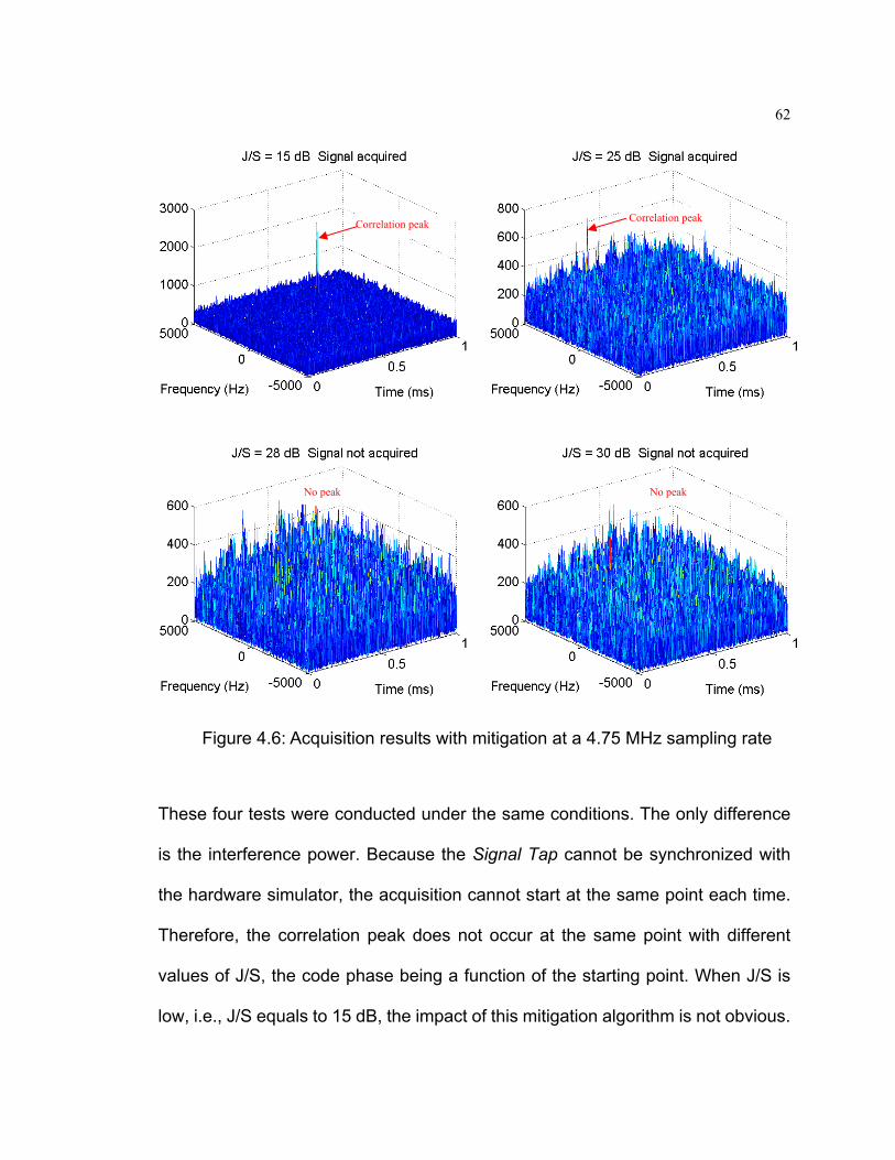
62
Figure 4.6: Acquisition results with mitigation at a 4.75 MHz sampling rate
These four tests were conducted under the same conditions. The only difference
is the interference power. Because the Signal Tap cannot be synchronized with
the hardware simulator, the acquisition cannot start at the same point each time.
Therefore, the correlation peak does not occur at the same point with different
values of J/S, the code phase being a function of the starting point. When J/S is
low, i.e., J/S equals to 15 dB, the impact of this mitigation algorithm is not obvious.
Correlation peak
No peak
Correlation peak
No peak

63
Although the mitigation algorithm can remove the sinusoidal oscillation of the
correlation value, the acquisition result is the same compared with no mitigation.
In both cases, the correlation peak stands out well against the noise. When the
J/S reaches 25 dB, the correlation peak is buried into the oscillation without
mitigation. On the contrary, this algorithm can effectively remove the oscillation
and correctly ascertain the correlation peak.
Table 4.2 shows the peak value versus noise floor and SNR under different
interference power conditions.
Table 4.2: Peak value versus noise floor and SNR
J/S (dB) Peak value Noise floor SNR (ratio) 15 2205.9 166.1 13.3 25 735.3 103.4 7.1 28 598.8 82.4 7.2 30 552.7 79.8 6.9
No interference 2723.7 200.3 13.6 Note: no units for peak value and noise floor
With the use of the frequency excision algorithm, the interference frequency
component was removed but, at the same time, parts of the signal component
and noise component have been removed as well. Thus, it can be seen from
Table 4.2 that the peak values and noise floors were reduced when this mitigation
algorithm was applied. The higher the value of J/S, the more interference is
associated with the signal. When J/S increases to a certain level, the frequency
property of the interference will not be distinguished from the signal by this
64
mitigation algorithm. As J/S continues to increase to 28 dB, the correlation peak
cannot be found even if this algorithm is applied. The mitigation ability of this
algorithm therefore is limited to scenarios where J/S is no more than 25 dB.
4.4 Mitigation result using a 7 MHz sampling rate
In this scenario, an intermediate frequency was sampled at 7 MHz with the use of
1 bit quantization. The other parameters are the same as in the 4.75 MHz
sampling scenario. The acquisition result with mitigation is shown in Figure 4.7:

65
Figure 4.7: Acquisition results with mitigation at a 7 MHz sampling rate
From the plots in Figure 4.7, it can be seen than when J/S increases to 28 dB,
signal acquisition is still possible. It is obvious that there is a 3 dB anti-jamming
improvement with a 7 MHz sampling rate compared with the 4.75 MHz sampling
rate. The cause of this phenomenon will be discussed in next section.
Correlation peak
Correlation peak
No peak
Correlation peak

66
4.5 Nyquist’s law and analysis of sampling rate on acquisition
4.5.1 Nyquist’s law
If the highest frequency contained in an analog signal )t(aX is WFmax = and
the signal is sampled at a rate W2F2F maxs => , then )t(aX can be exactly
recovered from its sample values. When the sampling of )t(aX is performed at
the minimum sampling rate W2Fs = , the reconstruction formula is as follows
[Proakis, 1996]:
)W2/nt(Wπ2)W2/nt(Wπ2sin)
W2n(x)t(x
naa −
−∑=∞
−∞= (4.5)
The sampling rate of W2Fs = is called the Nyquist’s rate.
From the Fourier theory aspect, the ideal sampling function is:
)nff(δf)mTt(δn
ssm
s ∑ −⇔∑ −∞
−∞=
∞
−∞= (4.6)
Equation 4.4 states that the Fourier transform of a periodic train of delta functions,
spaced sT seconds apart, consists of another set of delta functions weighted by
the factor ss T/1f = and regularly spaced sf Hz apart along the frequency axis.
Sampling is equivalent to multiplying a signal by a train of delta functions
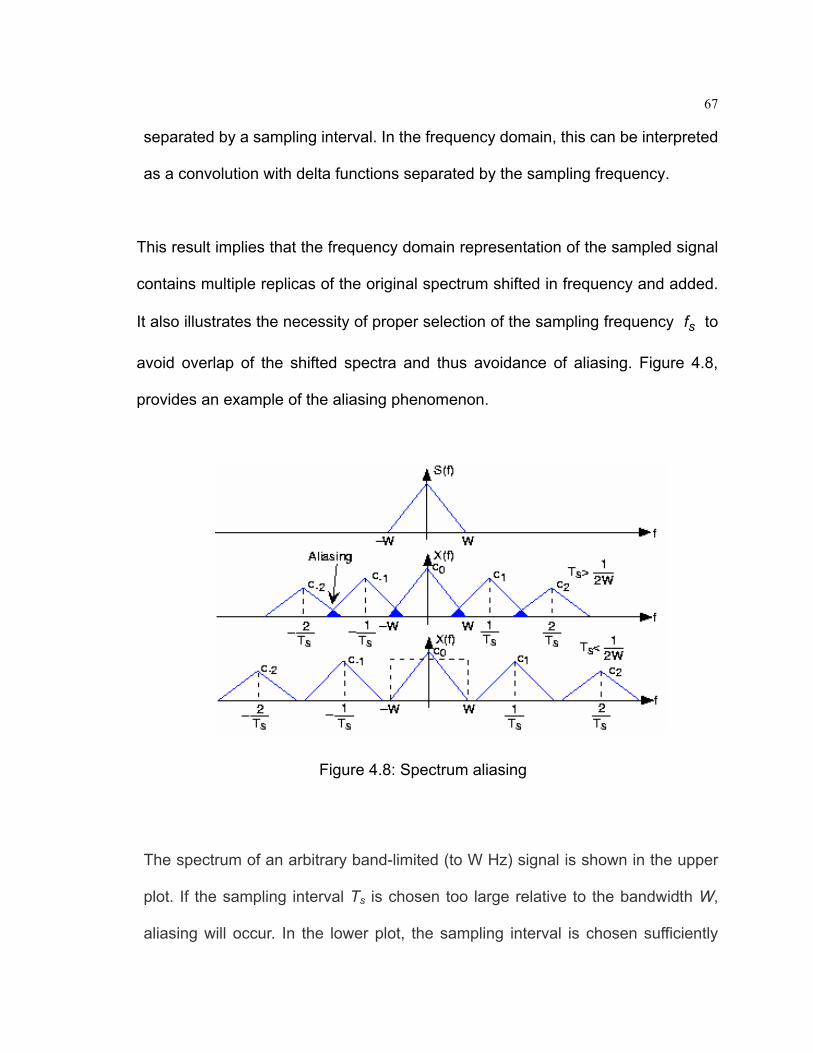
67
separated by a sampling interval. In the frequency domain, this can be interpreted
as a convolution with delta functions separated by the sampling frequency.
This result implies that the frequency domain representation of the sampled signal
contains multiple replicas of the original spectrum shifted in frequency and added.
It also illustrates the necessity of proper selection of the sampling frequency sf to
avoid overlap of the shifted spectra and thus avoidance of aliasing. Figure 4.8,
provides an example of the aliasing phenomenon.
Figure 4.8: Spectrum aliasing
The spectrum of an arbitrary band-limited (to W Hz) signal is shown in the upper
plot. If the sampling interval Ts is chosen too large relative to the bandwidth W,
aliasing will occur. In the lower plot, the sampling interval is chosen sufficiently

68
small to avoid aliasing. Note that, if the signal were not band-limited, the
component spectra would always overlap.
From Figure 4.8, it is clear that the bandwidth of the signal plays an important role
in correctly choosing the sampling frequency. Here attention should be paid that it
is the bandwidth of the signal and not the signal’s frequency that plays this
important role in choosing sampling frequency.
4.5.2 Analysis of sampling rate on acquisition
A 2 MHz filter is used in the second down-conversion stage of the Signal Tap,
resulting in an IF spectrum between 14.42 MHz and 16.42 MHz. According to the
sampling theory mentioned in the previous section, if the IF bandwidth is 2 MHz,
then a 4.75 MHz sampling rate is suitable. However, in reality, the filters in the
Signal Tap are composed of tuned circuits and sudden transitions from infinite to
zero attenuation are not possible. The sharper the required cutoff, the more
expensive and the more bulky the filter becomes. Also, realistic filter components
have a finite thermal coefficient such that the passband of the filter must be
widened to allow for this thermal variation. Hence it is difficult to meet the ideal
characteristics that are required to provide a very fine separation between the
replica spectra.
Based on the analysis above, it can be concluded that aliasing is irreversible and

69
can be prevented only by attenuating high frequency content before the sampling
process. To prevent aliasing completely, a perfect filter that passes all energy
from DC to the highest frequency of interest and rejects all energy at and above
the Nyquist frequency is needed. Unfortunately, perfect filters are not physically
realizable in analog or digital form. Physically realizable filters must have
variations in the passband, a smooth transition from the passband to the
stopband, and finite attenuation in the stopband. Note that finite attenuation
means that one cannot eliminate aliasing, but only reduce it. If the sampling rate is
increased, the requirement for the filter will be lower. Therefore, the variation and
dispersion of the filter will have less impact on the performance of ADC. That is
the reason why the high sampling rate provides better performance in this
application.
4.6 Influence of coherent integration time on interference
mitigation
Coherent integration is also called pre-detection integration [Ray, 2003].
Pre-detection is the phase of signal processing that occurs after the IF signal has
been converted to base band by the carrier- and code-stripping processes, but
prior to being passed through a signal discriminator, i.e. prior to the nonlinear
signal detection process.
Coherent integration time determines the shape of the frequency response of the

70
correlation triangle. The span of the correlation triangle is between –T to +T,
where T is the code chip width and the span of the main lobe of the Sinc curve is
between cf− and cf+ where [Kaplan, 1996]
Period_ectiondetePr1fc = (4.7)
For example, for a prediction period of 4 ms, the first null point of the Sinc curve is
at +/- 250 Hz. Thus, the coherent correlation time must be as long as possible to
operate under weak or RFI signal conditions, in order to obtain a higher
correlation gain. It must be as short as possible to operate under high-dynamic
stress signal conditions. Thus the pre-detection integration time is a compromise
design. However, during initial acquisition period, the receiver does not know
where the navigation data bit transition boundaries are located. So another limit of
coherent integration time is that it cannot exceed 20 ms, which is the 50 Hz
navigation message data period. The plots in Figure 4.9 show the different
acquisition results under different coherent integration times where a 7 MHz
sampling rate is used.

71
Figure 4.9: Impact of coherent time on mitigation results
Correlation peak
Correlation peak Correlation peak
Correlation peak Correlation peak
No peak
72
In this scenario, J/S is set to 28 dB, which is relatively high, in order to show the
impact of coherent time on mitigation results. As can be seen from the plots in
Figure 4.9, no correlation peak appears if the integration time equals 4 ms.
When coherent integration time reaches 6 ms, the algorithm reports that the
signal has been acquired. But the acquired Doppler and code delay is apparently
not correct; the acquisition results should be same, since these results were from
the same data set. At least an 8 ms integration time is needed to correctly acquire
the signal. With a high level of interference, the longer the coherent integration
time, the better the mitigation results on acquisition. It is not surprising to see that
the best mitigation result can be achieved when coherent integration time reaches
20 ms.
4.7 Conclusion
For low level interference (i.e., J/S less than 15 dB), a GPS receiver can use its
inherent anti-jamming property of spread spectrum to acquire the signal. For high
level interference, spectrum analysis is a useful tool to mitigate interference. The
maximum tolerance of effectively mitigating CW interference in acquisition when
using this algorithm can reach 28 dB of J/S if a high sampling rate and a long
coherent integration time are employed.

73
CHAPTER 5
Mitigation Analysis in Tracking and Position
5.1 CW interference mitigation results in tracking
In this scenario, 10 seconds of data was collected and interference was applied
after 4 seconds from the starting point. The In-phase prompt (IP) component,
Doppler accuracy and estimated C/N0 were compared. There are two reasons
why interference was applied after 4 seconds:
1) To ensure that the acquisition is processed under a clean environment so that
the tracking error is isolated.
2) To ensure convergence of the tracking process before commencing the
performance comparison. Thus, the impact of interference is only on tracking.
5.1.1 IP component mitigation results
The plots in Figure 5.1 show the IP component from the correlator output with a
sampling rate of 4.75 MHz.

74
Figure 5.1: IP component comparison
In Figure 5.1, results without mitigation are shown on the left hand side plots,
while the right hand side plots depict the results with mitigation. For low J/S (i.e.,
J/S equals 15 dB) CW interference has no influence on the output of the IP
component and the mitigation algorithm provides no improvement to the tracking
results. Besides that, the correlation output reduces significantly due to loss of the
0 1000 2000 3000 4000 5000 6000 7000 8000 9000 10000-800
-600
-400
-200
0
200
400
600
800Sampling Rate:4.75M J/S=25dB with mitigation
time(ms)
IP c
ompo
nent
s
0 1000 2000 3000 4000 5000 6000 7000 8000 9000 10000-800
-600
-400
-200
0
200
400
600
800Sampling Rate:4.75M J/S=25dB w/o mitigation
time(ms)
IP c
ompo
nent
s
0 1000 2000 3000 4000 5000 6000 7000 8000 9000 10000-800
-600
-400
-200
0
200
400
600
800Sampling Rate:4.75M J/S=15dB with mitigation
time(ms)
IP c
ompo
nent
s
0 1000 2000 3000 4000 5000 6000 7000 8000 9000 10000-800
-600
-400
-200
0
200
400
600
800Sampling Rate:4.75M J/S=15dB w/o mitigation
time(ms)
IP c
ompo
nent
s

75
signal component as a consequence of application of the frequency excision
algorithm.
When interference power is high (i.e., J/S equals 25 dB) the improvement with
use of the mitigation algorithm is apparent. The data bit transition is clear and the
navigation data can be decoded thereafter compared with the noise only output
without mitigation. The improvement is limited to 30 dB of J/S; if greater than that,
the correlator output consists only of noise, even if the mitigation algorithm is
applied.
The sampling rate still plays an important role in tracking. When the sampling rate
is increased from 4.75 MHz to 7 MHz, the maximum J/S is 35 dB for this algorithm
to take effect in tracking. There is a 5 dB improvement, as compared with a 4.75
MHz sampling rate.
The IP component is only a coarse descriptor of the GPS data. Here the
maximum tolerance for the mitigation algorithm means that the software receiver
can obtain the data bit, but this cannot be guaranteed to be 100 percent correct.
Whether it can pass through bit synchronization and preamble checking is
investigated in Chapter 6.
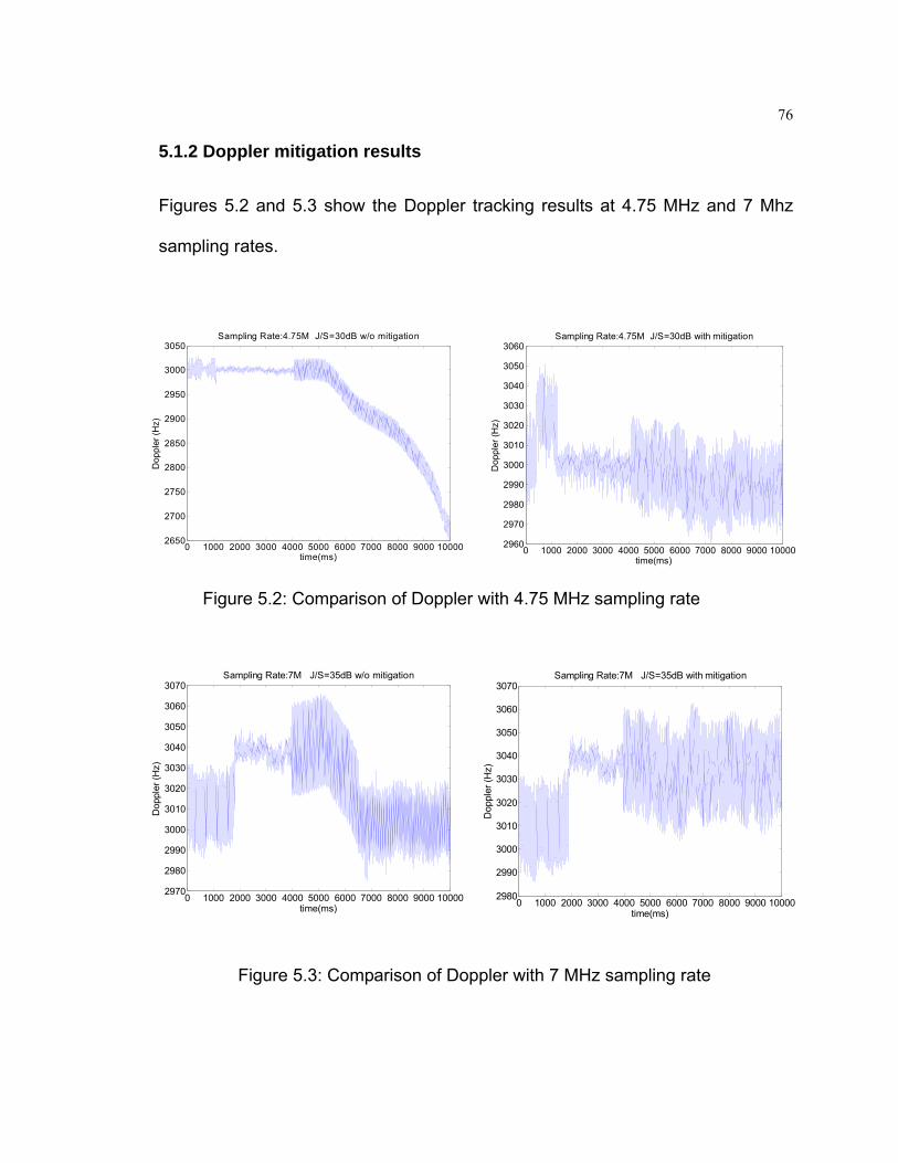
76
5.1.2 Doppler mitigation results
Figures 5.2 and 5.3 show the Doppler tracking results at 4.75 MHz and 7 Mhz
sampling rates.
Figure 5.2: Comparison of Doppler with 4.75 MHz sampling rate
Figure 5.3: Comparison of Doppler with 7 MHz sampling rate
0 1000 2000 3000 4000 5000 6000 7000 8000 9000 100002980
2990
3000
3010
3020
3030
3040
3050
3060
3070Sampling Rate:7M J/S=35dB with mitigation
time(ms)
Dop
pler
(Hz)
0 1000 2000 3000 4000 5000 6000 7000 8000 9000 100002960
2970
2980
2990
3000
3010
3020
3030
3040
3050
3060Sampling Rate:4.75M J/S=30dB with mitigation
time(ms)
Dop
pler
(Hz)
0 1000 2000 3000 4000 5000 6000 7000 8000 9000 100002970
2980
2990
3000
3010
3020
3030
3040
3050
3060
3070Sampling Rate:7M J/S=35dB w/o mitigation
time(ms)
Dop
pler
(Hz)
0 1000 2000 3000 4000 5000 6000 7000 8000 9000 100002650
2700
2750
2800
2850
2900
2950
3000
3050Sampling Rate:4.75M J/S=30dB w/o mitigation
time(ms)
Dop
pler
(Hz)
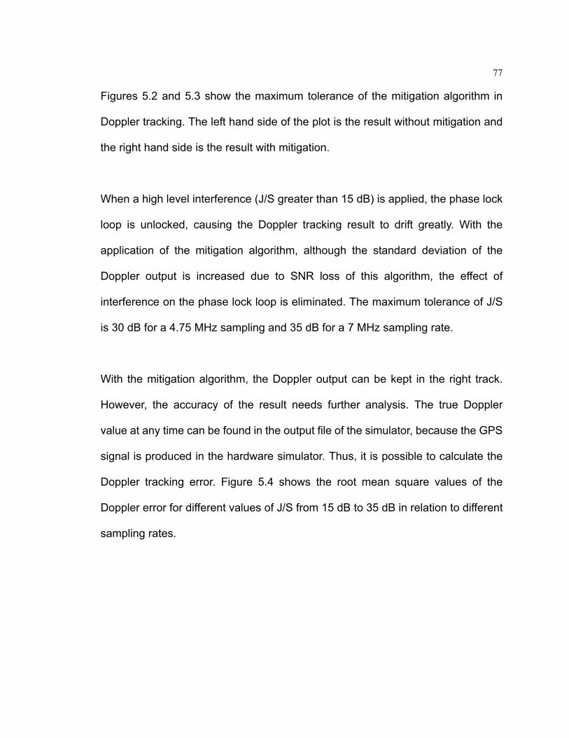
77
Figures 5.2 and 5.3 show the maximum tolerance of the mitigation algorithm in
Doppler tracking. The left hand side of the plot is the result without mitigation and
the right hand side is the result with mitigation.
When a high level interference (J/S greater than 15 dB) is applied, the phase lock
loop is unlocked, causing the Doppler tracking result to drift greatly. With the
application of the mitigation algorithm, although the standard deviation of the
Doppler output is increased due to SNR loss of this algorithm, the effect of
interference on the phase lock loop is eliminated. The maximum tolerance of J/S
is 30 dB for a 4.75 MHz sampling and 35 dB for a 7 MHz sampling rate.
With the mitigation algorithm, the Doppler output can be kept in the right track.
However, the accuracy of the result needs further analysis. The true Doppler
value at any time can be found in the output file of the simulator, because the GPS
signal is produced in the hardware simulator. Thus, it is possible to calculate the
Doppler tracking error. Figure 5.4 shows the root mean square values of the
Doppler error for different values of J/S from 15 dB to 35 dB in relation to different
sampling rates.
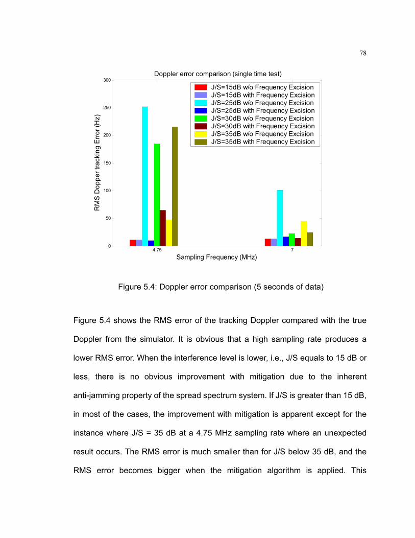
78
4.75 70
50
100
150
200
250
300
RM
S D
oppe
r tra
ckin
g E
rror (
Hz)
Sampling Frequency (MHz)
Doppler error comparison (single time test)
J/S=15dB w/o Frequency ExcisionJ/S=15dB with Frequency ExcisionJ/S=25dB w/o Frequency ExcisionJ/S=25dB with Frequency ExcisionJ/S=30dB w/o Frequency ExcisionJ/S=30dB with Frequency ExcisionJ/S=35dB w/o Frequency ExcisionJ/S=35dB with Frequency Excision
Figure 5.4: Doppler error comparison (5 seconds of data)
Figure 5.4 shows the RMS error of the tracking Doppler compared with the true
Doppler from the simulator. It is obvious that a high sampling rate produces a
lower RMS error. When the interference level is lower, i.e., J/S equals to 15 dB or
less, there is no obvious improvement with mitigation due to the inherent
anti-jamming property of the spread spectrum system. If J/S is greater than 15 dB,
in most of the cases, the improvement with mitigation is apparent except for the
instance where J/S = 35 dB at a 4.75 MHz sampling rate where an unexpected
result occurs. The RMS error is much smaller than for J/S below 35 dB, and the
RMS error becomes bigger when the mitigation algorithm is applied. This

79
phenomenon is due to the short data analysis period. In this test scenario, only 5
seconds of data was analyzed in order to save processing time; in the process,
random factors have apparently dominated the result. So In order to remove the
effects of random factors, a longer analysis period and a stochastic repeatability
test are needed.
Figure 5.5 shows the result of the average of six tests with different J/S values.
Each time, the tracking process lasts for 30 seconds.
4.75 70
50
100
150
200
250
300
RM
S D
oppe
r tra
ckin
g E
rror (
Hz)
Sampling Frequency (MHz)
Doppler error comparison (average of 6 times test)
J/S=15dB w/o Frequency ExcisionJ/S=15dB with Frequency ExcisionJ/S=25dB w/o Frequency ExcisionJ/S=25dB with Frequency ExcisionJ/S=30dB w/o Frequency ExcisionJ/S=30dB with Frequency ExcisionJ/S=35dB w/o Frequency ExcisionJ/S=35dB with Frequency Excision
Figure 5.5: Doppler error comparison (30 seconds of data)
These results are more reasonable than the single test results shown in Figure

80
5.4. Without mitigation, the Doppler error is not proportional to the interference
level. Under this condition, the tracking loop is divergent and the GPS receiver
loses lock on the Doppler.
With mitigation, the Doppler error is much smaller than the results observed
without mitigation and this error is proportional to the interference level. The only
exception is where the J/S equals 35 dB with a 4.75 MHz sampling rate. The RMS
error is greater than without mitigation. In this case, the interference level actually
exceeds the maximum tolerance of the mitigation algorithm with a 4.75 MHz
sampling rate. The mitigation algorithm is not reliable under this condition, thereby
requiring use of a high sampling rate. For a J/S of 35 dB with a 7 MHz sampling
rate, the mitigation algorithm is still effective in tracking. The Doppler error is
restricted to a reasonable level and the overall RMS error of 7 MHz sampling is
smaller than with for 4.75 MHz sampling. These results are from the average of
six tests and can be said to be statistically repeatable.
5.1.3 Estimated C/N0
In practice, the ratio of total carrier power to the noise density C/N0 in dB-Hz is the
most generic representation of signal power as it is independent of the
implementation of the receiver front-end bandwidth. C/N0 can also be used as the
lock detector to indicate a loss of lock of the DLL. In a software receiver, the C/N0
measurement can be estimated as [Parkinson and Spilker, 1996]:

81
⎥⎦
⎤⎢⎣
⎡−
−=
NP
NP10
0 µM1µ
T1log10
NC
(5.1)
where
∑=−
K
1KKNP NP
K1µ (5.2)
( )k
M
1i
2i
2i
2
k
M
0ii
2
k
M
0ii
kQI
QINP
⎟⎟⎠
⎞⎜⎜⎝
⎛∑ +
⎟⎟⎠
⎞⎜⎜⎝
⎛∑+⎟⎟
⎠
⎞⎜⎜⎝
⎛∑
=
=
== (5.3)
M is the sample number.

82
.
Figure 5.6: C/N0 comparison
Figure 5.6 shows the improvement in C/N0 with mitigation. The mitigation result
follows the same trend as the Doppler results. For lower values of J/S, the
improvement is very small. Much improvement occurs for medium level
interference. For J/S greater than 15 dB, the C/N0 tends to be zero without
mitigation due to the loss of lock on DLL while, with mitigation, the estimated C/N0
is high enough to keep code and carrier locked. The higher the sampling rate, the
better the C/N0 estimation is. In the interference level of 35 dB of J/S, a 7 MHz
sample provides a good C/N0 estimation while a 4.75 MHz sample produces total
loss of lock.
4.75 70
5
10
15
20
25
30
35
40
45
C/N
0 E
stim
ated
(dB
)
Sampling Frequency (MHz)
Estimated C/N0 Comparison
J/S=15dB w/o Frequency Excision
J/S=15dB with Frequency Excision
J/S=25dB w/o Frequency Excision
J/S=25dB with Frequency Excision
J/S=30dB w/o Frequency Excision
J/S=30dB with Frequency Excision
J/S=35dB w/o Frequency Excision
J/S=35dB with Frequency Excision

83
5.2 CW Interference mitigation results in position domain
5.2.1 Benchmarks for performance analysis in the position domain
In the position domain test, all error sources have been turned off except noise.
The impact of non-removable random noise in the hardware simulator and Signal
Tap will be discussed in this section. The position error level under the noise-only
error source condition will be used as benchmark for interference mitigation
performance comparisons in the position domain. Figure 5.7 shows the horizontal
and vertical position errors under noise-only conditions.
135040 135050 135059 135069 135078 135088 135098 1351070
2
4
6
8
10
Pos
ition
erro
r (m
)
06:31 06:31 06:31 06:31 06:31 06:31 06:32 06:32GPS Time(s); Local Time(hh:mm)
Horizontal error RMS = 1.75 (m)Vertical error RMS = 1.18 (m)
Figure 5.7: Position errors under noise-only conditions
Due to the randomness of noise, a one-time test result is not enough. In order to

84
measure repeatability, the test was carried out six times under the same
conditions. Figure 5.8 shows the results of the six consecutive tests.
1 2 3 4 5 60
0.5
1
1.5
2
2.5
Sample number
Pos
ition
erro
r RM
S (m
)Horizontal error RMS mean = 1.76 (m)Vertical error RMS mean = 1.20 (m)
Figure 5.8: Position error comparison of 6 tests under noise-only conditions
It can be seen from Figure 5.8 that, when all the other error sources have been
removed except noise, the expected horizontal position RMS error is around 1.8
metres and the vertical RMS error around 1.2 metres (the PDOP is 1.9 and is
essentially constant over the scenario). When the mitigation algorithm is applied,
some of the signal frequency components will be removed, causing the distortion
in the correlation peak. So the expected position RMS error will increase. If the
RMS error can be kept below a reasonable level, the mitigation process is
successful. Otherwise, it will be declared a failure.
85
5.2.2 Warm and cold start
The mitigation performance in the position domain was analyzed under two
conditions: warm start and cold start. The definition of warm start in this thesis is
to start acquisition in a “clean” environment without any interference. Interference
is then applied after the convergence of signal tracking. By comparison, cold start
means that acquisition is started after the interference is applied. The reason of
setting these two scenarios lies in the fact that the required C/N0 differs for
acquisition and tracking.
The effects of RFI on code correlation and loop filtering are to reduce the C/N0 of
all of the GPS signals. If the C/N0 is reduced below the tracking threshold, the
receiver will lose its ability to obtain measurements from the satellites. As the line
of sight range to the source of RFI increases, the C/N0 increases. A good rule of
thumb for the acquisition threshold C/N0 for a GPS receiver is about 6 dB higher
than the tracking threshold [Kaplan, 1996]. If the receiver is jammed out of
tracking the GPS signals, the distance from the interference source must be
increased such that the effective C/N0 increases by about 6 dB before the GPS
receiver can reacquire again. This also means that, when the GPS signal is
acquired, even if the interference level increases, the receiver is still able to track
the signal. Stated another way, the impact on the position solution is not as
serious as that when the same level of interference occurs during the acquisition
period.
86
In warm start conditions, only the tracking procedure is under the interference
environment. The required C/N0 is lower than in cold start. The tolerance for
interference is thus higher, so the mitigation results should be different.
5.2.3 CW interference mitigation in the position domain
Due to the limited memory capacity of the Signal Tap, only 80 seconds of data
could be collected. The GPS position can be fixed only after the receiver collects
the required ephemeris. The first three sub-frames that last 18 seconds have to
be decoded in order to get the required ephemeris, so 60 seconds of position data
can be provided for analysis.
The software GPS receiver is nonlinear, especially near its tracking threshold. It is
very difficult to predict the tracking threshold for a given dynamic scenario. Only a
Monte Carlo simulation can assist in studying this phenomenon. Heuristic
techniques are usually used to predict the signal tracking threshold. For a
second-order loop with an 18 Hz noise bandwidth and a 20 ms pre-detection
integration time, the rule of thumb tracking threshold is 28 dB-Hz [Kaplan, 1996],
and this was the value used in this test. If the estimated C/N0 is below this
threshold, the receiver decides that the tracking process failed and the receiver
attempts to reacquire again.
Figure 5.9 compares the mitigation results in cold and warm start conditions. A

87
second order loop filter with 18 Hz noise bandwidth and a 20 ms pre-detection
integration time was used.
14 16 18 20 22 240
2
4
6
8
10
12po
sitio
n er
ror R
MS
(m)
J/S (dB)
Mitigation results comparison warm start (horizontal )
no mitigation RMS = 4.16 (m) with mitigation RMS = 4.78 (m)
17 18 19 20 21 22 230
2
4
6
8
10
12
Pos
ition
erro
r RM
S (m
)
J/S (dB)
Mitigation results comparison cold start (horizontal)
no mitigation with mitigation RMS = 5.42
Figure 5.9: Comparison of mitigation results with CW interference
It can be seen from Figure 5.9, when interference is applied, the position error

88
RMS increases. This is the expected result, because the mitigation algorithm also
removes part of the signal energy when the interference frequency component is
removed, causing distortion in the correlation peak. This increased position error
is caused by small pseudorange errors on all satellites.
In a warm start environment, no improvement in the position domain is observed
when the mitigation algorithm is applied. On the contrary, the horizontal root mean
square error is worse with mitigation. This is because when the interference
frequency component is excised, and some of the signal component has been
removed as well. At any interference level, the signal frequency component will
always mix with the interference frequency to a certain degree. If the interference
power level is not high, the inherent anti-jamming property of the spread spectrum
system can mitigate the interference without any extra processing. With mitigation,
due to the signal loss upon frequency excision, the resulting position solution is
slightly degraded.
Under cold start conditions, acquisition is performed in an interference
environment. As discussed before, acquisition requires C/N0 6 dB higher than
tracking. At the same level of interference, the inherent anti-jamming ability may
not be enough to enable acquisition. Unlike tracking, this level of interference may
cause acquisition problems. Incorrect acquisition results may cause divergence of
the tracking loop, making position fixing impossible or producing very a large
position error. Thus, in a cold start condition, the mitigation algorithm is essential.
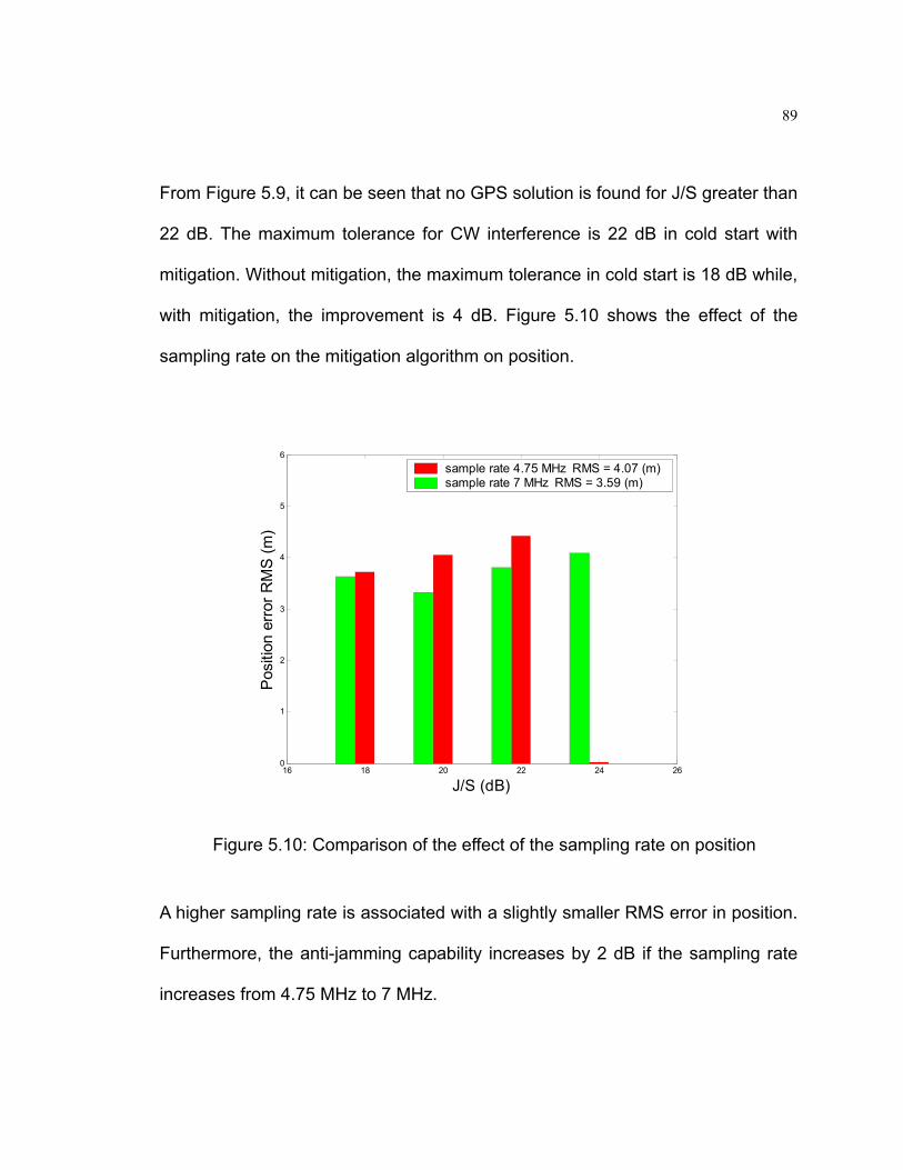
89
From Figure 5.9, it can be seen that no GPS solution is found for J/S greater than
22 dB. The maximum tolerance for CW interference is 22 dB in cold start with
mitigation. Without mitigation, the maximum tolerance in cold start is 18 dB while,
with mitigation, the improvement is 4 dB. Figure 5.10 shows the effect of the
sampling rate on the mitigation algorithm on position.
16 18 20 22 24 260
1
2
3
4
5
6
Pos
ition
err
or R
MS
(m)
J/S (dB)
sample rate 4.75 MHz RMS = 4.07 (m) sample rate 7 MHz RMS = 3.59 (m)
Figure 5.10: Comparison of the effect of the sampling rate on position
A higher sampling rate is associated with a slightly smaller RMS error in position.
Furthermore, the anti-jamming capability increases by 2 dB if the sampling rate
increases from 4.75 MHz to 7 MHz.
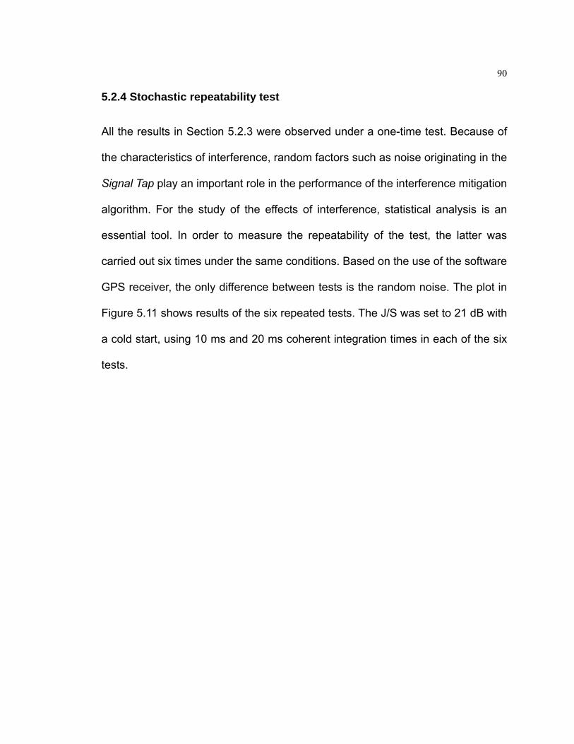
90
5.2.4 Stochastic repeatability test
All the results in Section 5.2.3 were observed under a one-time test. Because of
the characteristics of interference, random factors such as noise originating in the
Signal Tap play an important role in the performance of the interference mitigation
algorithm. For the study of the effects of interference, statistical analysis is an
essential tool. In order to measure the repeatability of the test, the latter was
carried out six times under the same conditions. Based on the use of the software
GPS receiver, the only difference between tests is the random noise. The plot in
Figure 5.11 shows results of the six repeated tests. The J/S was set to 21 dB with
a cold start, using 10 ms and 20 ms coherent integration times in each of the six
tests.
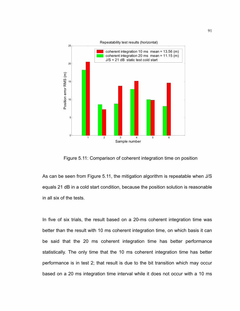
91
1 2 3 4 5 60
5
10
15
20
25
Pos
ition
erro
r RM
S (m
)
Sample number
Repeatability test results (horizontal)
coherent integration 10 ms mean = 13.56 (m) coherent integration 20 ms mean = 11.15 (m) J/S = 21 dB static test cold start
Figure 5.11: Comparison of coherent integration time on position
As can be seen from Figure 5.11, the mitigation algorithm is repeatable when J/S
equals 21 dB in a cold start condition, because the position solution is reasonable
in all six of the tests.
In five of six trials, the result based on a 20-ms coherent integration time was
better than the result with 10 ms coherent integration time, on which basis it can
be said that the 20 ms coherent integration time has better performance
statistically. The only time that the 10 ms coherent integration time has better
performance is in test 2; that result is due to the bit transition which may occur
based on a 20 ms integration time interval while it does not occur with a 10 ms
92
interval. During the acquisition period, no prior knowledge about the data bit
boundary is provided. Even the pre-detection integration time is limited to within
20 ms; there is still a chance that a data bit transition may occur.
For test 1, the error is larger than that of the other 5 samples due to the presence
of random noise. In test 1, the noise happens to be slightly larger than in other
tests and the mitigation algorithm amplifies it. This result occurs because higher
random noise mixes the interference spectrum more with the signal and makes
the mitigation algorithm excise more signal energy, thus causing more distortion in
the correlation peak and introducing a greater pseudorange error.
Figure 5.12 shows the rate of success in obtaining position solutions under
different interference levels when the mitigation algorithm is applied. If no position
can be calculated, or if the position error exceeds 50 metres (meaning that the
error is well above the normal value and the result is not reliable), the algorithm
declares a failure. A series of six tests were carried out at each interference level.

93
18 19 20 21 22 23 24 25 26 27 280
10
20
30
40
50
60
70
80
90
100
Suc
essf
ul ra
te (%
)
J/S (dB)
Rate of sucessful position fixing
cold startwarm start
Figure 5.12: Rate of successful position fixing
Under cold start conditions, when the J/S is no greater than 21 dB, the success
rate in obtaining a position solution is 100 percent. If the J/S increases to 22 dB or
23 dB, the success rate is reduced to 33.3 percent or 16.7 percent, respectively. If
the J/S continues to increase, no solution can be obtained. The mitigation
algorithm is statistically stable when the J/S is no greater than 21 dB in a cold start
condition.
In warm start conditions, when the J/S is no greater than 26 dB, a 100 percent
success rate in obtaining a solution can be achieved. If the J/S increases to 27 dB,
the success rate is reduced to 33.3 percent. If the J/S continues to increase, it is

94
not possible to obtain a solution. The mitigation algorithm is statistically stable
when the J/S is no greater than 26 dB under warm start conditions.
5.3 AM interference mitigation results in the position domain
Amplitude modulation (AM) is a method of impressing data onto an
alternating-current (AC) carrier waveform. The highest frequency of the
modulating data is normally less than 10 percent of the carrier frequency [Proakis,
1996a]. The instantaneous amplitude (overall signal power) varies depending on
the instantaneous amplitude of the modulating data.
Considering the modulating waveform is a sine function, the amplitude modulation
of a signal can be expressed as:
[ ] tωsintωcosK1α cmm+ (5.4)
where
cω = the angular frequency of the carrier
mω = angular frequency of the signal to be modulated
mK = modulation index
α = scalar notation for amplitude of the carrier

95
From Equation 5.4, it can be seen that an AM signal is determined by five
parameters:
• Signal level
• Centre frequency
• Wave form
• Frequency of the signal to be modulated, and
• Modulation depth
An Agilent ESG E4431B signal generator was used in this thesis to generate an
AM signal and a frequency modulation (FM) signal. In this signal generator, the
modulating waveform can be selected from sine, square, ramp or triangle forms.
The frequency of the modulating signal must be in the range of 0.0001 to 50 kHz.
The modulation depth is specified as a percentage, ranging from 0 to 100%
[Spirent, 2003b].
The AM signal frequency is fixed, while only the amplitude changes. In the
frequency domain, the impact of AM interference on the GPS signal spectrum is
similar to CW interference. Only the amplitude of the interference frequency
component is changing with the AM parameter, which means that the frequency
excision algorithm can be used to remove the AM interference.
However, the impact of different AM parameters on the effectiveness of the

96
mitigation algorithm is different. The plots in Figure 5.13 illustrate the impact of the
modulating signal frequency on mitigation results.
Figure 5.13: Impact of modulating signal frequency of AM interference on mitigation results
135040 135050 135059 135069 135078 135088 135098 135107-5
0
5
10
15
20
Pos
ition
Erro
r (m
)
Warm start no mitigation J/S: 22 dB frequency 10 Hz
06:31 06:31 06:31 06:31 06:31 06:31 06:32 06:32GPS Time(s); Local Time(hh:mm)
Horizontal error RMS = 4.59 (m) Vertical error RMS = 10.19 (m)
135040 135050 135059 135069 135078 135088 135098 1351070
2
4
6
8
10
12
14
16
18
20P
ositi
on E
rror (
m)
Warm start no mitigation J/S: 22 dB frequency 100 Hz
06:31 06:31 06:31 06:31 06:31 06:31 06:32 06:32GPS Time(s); Local Time(hh:mm)
Horizontal error RMS = 4.21 (m) Vertical error RMS = 9.78 (m)

97
The mitigation result is similar when the frequency of the modulating signal is
changed from 10 Hz to 100 Hz. The modulating signal frequency is relatively low
compared with the centre frequency. In the analysis period, the change in the AM
interference amplitude is very small, so that the modulating signal frequency does
not have much influence on the mitigation results of the GPS position solution.

98
Figure 5.14 shows the influence of the modulation depth of AM interference on
position.
Figure 5.14: Influence of modulation depth of AM interference on mitigation results
135045 135055 135064 135074-5
0
5
10
15
20
25
30
35
40
Pos
ition
Erro
r (m
)
Warm start no mitigation J/S: 22 dB modulation depth: 90%
06:31 06:31 06:31 06:31GPS Time(s); Local Time(hh:mm)
Horizontal error RMS = 5.88 (m) Vertical error RMS = 13.32 (m)
135040 135050 135059 135069 135078 135088 135098 135107-5
0
5
10
15
20
Pos
ition
Erro
r (m
)
Warm start no mitigation J/S: 22 dB modulation depth: 50%
06:31 06:31 06:31 06:31 06:31 06:31 06:32 06:32GPS Time(s); Local Time(hh:mm)
Horizontal error RMS = 4.51 (m) Vertical error RMS = 10.52 (m)

99
The modulation depth determines the amplitude of the AM signal. From Equation
5.3, it can be seen that, when the modulation depth is 100 percent, the peak value
of the AM signal will double. The increase of modulation depth is somehow like
the increase of AM interference power. When modulation depth increases from 50
percent to 90 percent, the RMS position error increases by 30 percent. In the case
of a modulation depth of 90 percent, it can be seen from the plot above that no
GPS solution can be fixed after a GPS time of 135078 seconds. This implies that
modulation depth plays an important role in the influence of AM interference,
perhaps even causing the loss of tracking in the tracking loop.
Figure 5.15 compares the mitigation results with AM interference under cold start
conditions.
Figure 5.15: Mitigation results comparison with AM interference
14 15 16 17 18 19 20 21 220
2
4
6
8
10
12
14
posi
tion
erro
r RM
S (m
)
J/S (dB)
mitigation results comparison cold start (horizontal error RMS )
no mitigation with mitigation RMS = 6.87 (m)
100
From the plot in Figure 5.15, it can be seen that no solution is achieved with a J/S
greater than 15 dB without the mitigation algorithm. The tests with mitigation have
not been carried out due to concerns over managing the workload for J/S = 16, 17,
18, and 19 dB. The maximum tolerance for AM interference is 15 dB without
mitigation under cold start conditions.
Using the mitigation algorithm, the maximum tolerance for AM interference is 21
dB. No solution can be obtained when the J/S is greater than 21 dB which
represents a 6 dB improvement achieved with the mitigation algorithm, as
compared with no mitigation. The mitigation algorithm is generally effective in
mitigating AM interference in cold start conditions.
5.4 FM interference mitigation results in the position domain
FM is a modulation in which the instantaneous frequency of a sine wave carrier is
caused to depart from the centre frequency by an amount proportional to the
instantaneous value of the modulating signal. In FM, the carrier frequency is
called the centre frequency. FM is a form of angle modulation. The mathematical
expression of an FM signal is as follows. If the instantaneous frequency varies
linearly with the modulating signal, the FM signal can be expressed as:
)t))t(kfωsin((α c + (5.5)

101
In the case of phase modulation, the phase of the carrier varies with the
modulation signal and, in the case of FM, the phase of the carrier varies with the
integral of the modulating signal. Thus, there is no essential difference between
phase and frequency modulation. The term FM is generally used to include both
modulation types. If the modulating waveform is assumed to be a sinusoidal
signal at a frequency mf , the frequency modulation of a signal can be expressed
as:
)t)))t(ωcos(kωsin((α mc + (5.6)
where
cω = the angular frequency of the carrier
mω = angular frequency of the signal to be modulated
k = maximum frequency deviation of the carrier, and
α = scalar notation for amplitude of the carrier
An FM signal is determined by five parameters as in the equation above:
• Signal level
• Centre frequency of the carrier
• Wave form
• Frequency of the signal to be modulated

102
• Frequency deviation
The deviation of the modulating signal is dependent upon the centre frequency of
the main signal. Table 5.1 shows the frequency limits versus three centre
frequency values [Spirent, 2003b].
Table 5.1: Frequency limits versus centre frequency
Centre Frequency (MHz) Lower Limit (kHz) Upper Limit (kHz)
500 0.05 5000 >500 to 1000 0.1 10000 >1000 to 2000 0.2 20000
The FM signal frequency is changing. In the frequency domain, the impact of FM
interference on the GPS signal spectrum is similar to that of swept CW
interference. The sweeping rate depends on the frequency of the signal to be
modulated and the frequency deviation. In the FFT analysis period, more
frequency components will exist compared with CW interference. Although the
frequency excision algorithm is still effective in removing the FM interference, the
performance will degrade. More signal energy will be cut off, causing a decrease
in the estimated C/N0. The extent of the degradation is proportional to the
frequency of the signal to be modulated and the frequency deviation, because the
number of interference components in the FFT analysis period is proportional to
the frequency of the signal to be modulated and the frequency deviation.

103
Table 5.2 shows the frequency of the signal to be modulated with respect to FM
interference on position. The central frequency of the FM interference is on the
carrier frequency of L1 with an associated frequency deviation of 100 KHz.
Table 5.2: Comparison of FM frequency on GPS position
Frequency to be
Modulated (Hz)
1 5 50 500 1000
Horizontal error RMS (m) 4.65 4.45 4.66 4.74 No solution
Vertical error RMS (m) 10.36 10.68 10.60 14.00 No solution
When the FM frequency is lower, the number of interference frequency lines in the
FFT analysis period will be lower. As shown in Table 5.2, there is no large
difference in the solution for different FM frequency values from 1 Hz to 50 Hz.
When the frequency increases to a few hundred Hz, the position error increases
rapidly and, eventually, the receiver will lose lock.
Figure 5.16 illustrates the influence of frequency deviation of FM interference on
the solution. The central frequency of the FM interference is on the carrier
frequency of L1 and the frequency to be modulated is 50 Hz.

104
Figure 5.16: Influence of frequency deviation of FM interference on position
135040 135050 135059 135069 135078 135088 135098 135107-5
0
5
10
15
20x 104
Pos
ition
Erro
r (m
)
warm start no mitigation frequency deviation: 500 khz
06:31 06:31 06:31 06:31 06:31 06:31 06:32 06:32GPS Time(s); Local Time(hh:mm)
Horizontal error RMS = 94488.47 (m) Vertical error RMS = 69168.95 (m)
135040 135050 135059 135069 135078 135088 135098 135107-10
-5
0
5
10
15
20
25
Pos
ition
Erro
r (m
)
warm start FM interference no mitigation frequency deviation: 100 khz
06:31 06:31 06:31 06:31 06:31 06:31 06:32 06:32GPS Time(s); Local Time(hh:mm)
Horizontal error RMS = 4.66 (m) Vertical error RMS = 10.60 (m)

105
When the frequency deviation is small, for example, the narrow-band FM
interference with a frequency deviation within 100 KHz, the frequency deviation
has very little influence on position. The RMS error stands at the same level as
that for the CW interference with the same interference power. If the bandwidth of
FM interference becomes wide, for example, when the frequency deviation is set
to 500 KHz, the position error becomes extremely large. The frequency deviation
plays an important role on the influence of FM interference on GPS position
solution.

106
.
135040 135050 135059 135069 135078 135088 135098 1351070
10
20
30
40
50
60
70
13:31 13:31 13:31 13:31 13:31 13:31 13:32 13:32
GPS Time(s); Local Time(hh:mm)
Pos
ition
erro
r (m
)
J/S = 20 dB cold start with mitigation
Horizontal error RMS = 5.60 (m) Vertical error RMS = 11.19 (m)
135048 135052 135055 135059 135062 1350660
10
20
30
40
50
60
70
13:31 13:31 13:31 13:31 13:31 13:31
GPS Time(s); Local Time(hh:mm)
Pos
ition
erro
r (m
)
J/S = 21 dB cold start with mitigation
Horizontal error RMS = 13.17 (m) Vertical error RMS = 13.30 (m)
Figure 5.17: Mitigation results with FM interference

107
Figure 5.17 illustrates the mitigation results with FM interference. The parameters
of FM interference are established for test purposes as follows:
• centre frequency: GPS L1
• frequency deviation: 100 KHz, and
• modulate frequency: 5 Hz
Under this FM configuration, when the J/S equals 20 dB, the position error is
stable and restricted to a reasonable level. When J/S increases to 21 dB, the
position error increases rapidly and, after GPS time of 135066 seconds, no
position can be obtained. This implies that the receiver loses lock in the tracking
loops.
The maximum tolerance for this mitigation algorithm to take effect for FM
interference is defined by a J/S of 20 dB for 100 kHz while, without use of the
mitigation algorithm, the maximum tolerance of the software receiver is a J/S of 15
dB. Thus, the tolerance increases by 5 dB with the use of the mitigation algorithm
under cold start conditions.
If the modulation frequency or frequency deviation increases, the maximum
tolerance will also decrease, because a greater amount of signal energy will be
excised by the mitigation algorithm, causing FM interference to be more of a
problem than AM interference on the GPS receiver. At the medium modulation

108
level, the maximum tolerance of this mitigation algorithm for FM interference is
one dB lower than for AM interference.

109
CHAPTER 6
Kinematic Tests
6.1 Test setup
The kinematic mode was simulated using a combination of the hardware
simulator and SimGEN software. A simple motion model was used that allows the
user to specify constant speed motion in a perfect circle about a fixed point. The
vehicle describes a perfectly flat circle in the local geographic plane and, as the
earth is curved this will produce slight variations in height above the ellipsoid as
the vehicle traverses the circle. This effect will increase with circle radius. In this
test, the circle radius was set to 1000 m, so that the variation in height is very low.
6.2 Results and analysis
To investigate the impact of integration time in the loop filters on the solution in
dynamic and under interference conditions, the test was set to constant velocity at
80 m/s which simulates the high dynamic experienced in land vehicles, with a J/S
of 21 dB. Integration times of 1 ms, 2 ms, 4 ms and 6 ms were tested, with the
results shown in Table 6.1:

110
Table 6.1: Impact of integration time in loop filters on position errors
Integration time
(ms)
1 ms 2 ms 4 ms 6 ms
Horizontal RMS
error (m)
1066097.1 216309.5 278293.4 15.5
Vertical RMS error
(m)
222133.3 50233.7 888585.7 6.0
Satellites been
tracked
1,14,16,25 1,14,16,20,
25,30
11,14,20,
25,30
14,16,25,
30
As shown in Table 6.1, 6 ms of integration time can successfully mitigate the
influence of interference and yield a reasonable solution. But only four satellites
can be tracked, constituting a low availability. In this case, a long integration time
causes a low dynamic capability. If the integration time is reduced to 2 ms or 4 ms,
dynamic capability has been improved and six satellites can be tracked. But a
large position error exists due to the impact of interference. Under interference
conditions, the signal is weak and longer integration time is needed. If the problem
of large position error can be solved, both high accuracy and an acceptable level
of availability can be achieved.
The large position error is caused by the tracking of one or more satellites that

111
may have sizeable range errors. Figure 6.1 shows the pseudorange errors of
different satellites using 2 ms integration time.
Figure 6.1: Pseudorange errors compared with true value
In this situation, an integration time of 2 ms allows the tracking of six satellites.
However, the pseudoranges cannot converge to their true values after a least
squares (LS) adjustment. One large pseudorange error exists and this
measurement carries the same weight (due to the limitation of the current version
of software receiver) in the least squares solutions, causing divergence of the
112
estimation results. This error however could be removed using a fault detection
and exclusion algorithm if sufficient measurement redundancy is available.
Before the least squares adjustment, the pseudorange error is due to the clock
error. This error should be in the same scale for different satellites because they
use the same simulated inner clock. From Figure 6.1, it is obvious that satellite 20
is abnormal. PRN 20 is offset from the others by about 600 km which represents a
2 ms transmission time error. This error is an integer millisecond error caused by
the bit synchronization error, because one bit synchronization error produces a
one millisecond error in a pseudorange measurement. If the bit synchronization
result has a two bit offset from the true value, this error will exist throughout the
succeeding pseudorange calculation process. That is to say, if the signal is not
re-acquired again, this error will continue to persist. In order to eliminate this error,
further investigation into the bit synchronization process is needed.
The histogram approach is used to perform bit synchronization in the software
GPS receiver. This approach breaks a data bit period (20 ms) into 20 C/A-code 1
ms epoch periods and senses sign changes between successive epochs. For
each sensed sign change, a corresponding histogram cell count is incremented
until a count in one specific cell exceeds the other 19 bins by a pre-specified
amount.

113
The detection procedure can be described as follows [Parkinson and Spilker,
1996]:
1) A cell counter cellK is arbitrarily set and runs from 0 to 19.
2) Each sensed sign change is recorded by adding 1 to the histogram cell
corresponding to cellK
3) The process continues until one of the following occurs:
(a) Two cell counts exceed threshold 2T
(b) Loss of lock
(c) One cell count exceeds threshold 1T
4) If (a) occurs, the bit synchronization fails and is reinitialized. If (b) occurs,
one tries to reestablish lock. If (c) occurs, bit synchronization is successful,
and the C/A-code epoch count is reset to the correct value.
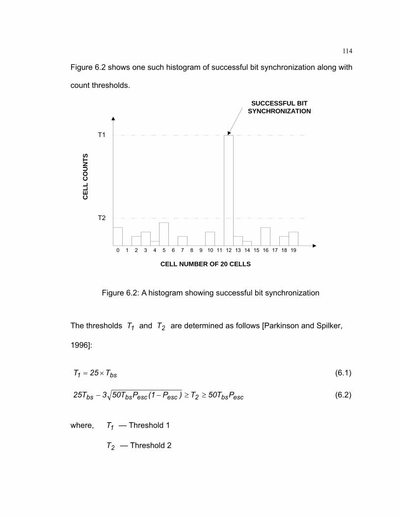
114
Figure 6.2 shows one such histogram of successful bit synchronization along with
count thresholds.
Figure 6.2: A histogram showing successful bit synchronization
The thresholds 1T and 2T are determined as follows [Parkinson and Spilker,
1996]:
bs1 T25T ×= (6.1)
escbs2escescbsbs PT50T)P1(PT503T25 ≥≥−− (6.2)
where, 1T — Threshold 1
2T — Threshold 2
0 19181716151413121110987654321
T1
T2
CELL NUMBER OF 20 CELLS
CEL
L C
OU
NTS
SUCCESSFUL BITSYNCHRONIZATION

115
bsT — Bit synchronization duration
escP — Probability of making an error in determining a sign change at
a desired C/N0
From the above discussion it is clear that, under interference conditions, there
exists the possibility that one bin may exceed the threshold 1 while the true bin is
still under threshold 2 due to the interference effect, causing the data bit to be
synchronized at the wrong bin. Figure 6.3 shows the bit synchronization result for
PRN 20.

116
Figure 6.3: Bit synchronization result for PRN 20
It can be seen that only cell 17 exceeds threshold 2, and it is the only cell to reach
threshold 1. Through a detection procedure, the bit synchronization process is
declared to be successful and the data bit transition point is assumed to be at cell
17 which is 2 bins away from the true value of cell 15.
The true bit synchronization point can be found from the warm start tracking
results. This is because the warm start and cold start are from the same data set
and only a few points are skipped for cold start processing. The data bit transition
point should be the same. However, the bit synchronization result from a warm
0 1 2 3 4 5 6 7 8 9 10 11 12 13 14 15 16 17 18 19 200
5
10
15
20
25
30
Cel
l cou
nts
Cell number of 20 cells
Histgram of bit synchronization (cold start J/S = 21 dB)
Threshold 1
Threshold 2
true synchronized bit

117
start is as shown in Figure 6.4.
Figure 6.4: Histogram of bit synchronization in warm start
The synchronization result has 2 cells offset from the true point. To improve bit
synchronization performance, the following two methods can be used:
1) Use a soft threshold for threshold 2. This threshold is associated with the
noise floor. If the noise level is high, the threshold will be lower. There will
be a high possibility of two cells exceeding threshold 2 before one cell
exceeds threshold 1. The bit synchronization will restart again instead of a
0 1 2 3 4 5 6 7 8 9 10 11 12 13 14 15 16 17 18 19 200
5
10
15
20
25
30C
ell c
ount
s
Cell number of 20 cells
Histogram of bit synchronization (warm start)

118
bit being synchronized at an incorrect point.
2) If 2 cells exceed threshold 2, go back to acquisition instead of starting bit
synchronization again, because the required acquisition C/N0 is about 6
dB higher than tracking. The bit synchronization error is most probably
caused by an inaccurate acquisition result. If acquisition is re-started, the
acquisition detection threshold can be adjusted through the newly
calculated noise floor. The acquisition result will be more precise and there
is a high possibility that the bit synchronization result will be true.
Figure 6.5 shows the bit synchronization result with the improved procedure.
The synchronized bit transition point is at the correct place.

119
0 1 2 3 4 5 6 7 8 9 10 11 12 13 14 15 16 17 18 19 200
5
10
15
20
25
30
Cel
l cou
nts
Cell number of 20 cells
Threshold 1
Threshold 2
True synchronized bit
Figure 6.5: Histogram of bit synchronization using the improved procedure
Figure 6.6 shows the pseudorange measurement error when using the improved
bit synchronization procedure. After the least squares adjustment, the errors of all
the satellites converge to their true values.

120
Figure 6.6: Pseudorange error using improved bit synchronization procedure
Figure 6.7 below shows the stochastic repeatability test results under kinematic
mode with frequency excision mitigation algorithm and improved bit
synchronization procedure (J/S 21 dB, velocity 80 m/s, and cold start).

121
Figure 6.7: Stochastic repeatability test results under kinematic mode
18 19 20 21 22 23 240
10
20
30
40
50
60
70
80
90
100
Suc
essf
ul ra
te (%
)
J/S (dB)
Rate of sucessful position fixing
V = 80 m/s
1 2 3 4 5 60
5
10
15
20
25
30
35
40
45
posi
tion
erro
r RM
S (m
)
Sample number
Comparison of coherent integration time on position (horizontal)
coherent integration 10 ms mean = 26.53 (m) coherent integration 20 ms mean = 14.51 (m) J/S = 21 dB V = 80 m/s
122
The results show that, when J/S is below 21 dB, the position error is stable and
restricted to within 10 metres. The success rate of obtaining position is 100
percent.
When the J/S increases to 21 dB, the position error varies but can still be
restricted to within 25 metres; the success rate of obtaining a correct position is
also 100 percent. When J/S increases to 22 dB, the success rate of obtaining a
correct position is reduced to 33.3 percent. If J/S is greater than 22 dB, a position
cannot be obtained. A 20 ms coherent integration time has better performance
statistically. The frequency excision algorithm with improved acquisition based on
bit synchronization result is statistically stable when the J/S is no greater than 21
dB under high dynamic conditions.

123
CHAPTER 7
Application of Data Window in FFT-based Mitigation Algorithm
7.1 The advantage of using a data window
In the previous chapters, the traditional FFT-based frequency excision
interference mitigation algorithm has been discussed. This method can remove
most of the interference energy in the frequency domain. The drawback is that it
can suppress energy only in the main-lobe spectral bins which is not adequate
due to the residual interference distributed throughout the spectrum by these
side-lobes, especially when interference power level is high.
FFT operations assume a periodic extension of a finite sequence that is to be
transformed. For each block of pN samples of the input sequence which is used
to do FFT analysis, if the pN samples are not periodic in the FFT’s window of
observation, a discontinuity occurs at the FFT’s block boundary. So the FFT of a
signal often exhibits high spectral side-lobes due to the finite aperture processing
interval. The behavior of these side-lobes is much like a broad band interference
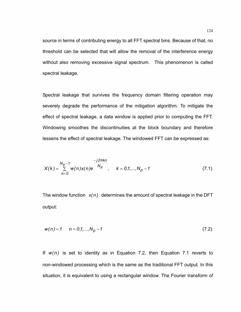
124
source in terms of contributing energy to all FFT spectral bins. Because of that, no
threshold can be selected that will allow the removal of the interference energy
without also removing excessive signal spectrum. This phenomenon is called
spectral leakage.
Spectral leakage that survives the frequency domain filtering operation may
severely degrade the performance of the mitigation algorithm. To mitigate the
effect of spectral leakage, a data window is applied prior to computing the FFT.
Windowing smoothes the discontinuities at the block boundary and therefore
lessens the effect of spectral leakage. The windowed FFT can be expressed as:
1N,...,1,0k,e)n(x)n(w)k(X1N
0np
Nknπ2j
pp −∑ ==
−
=
−
(7.1)
The window function )n(x determines the amount of spectral leakage in the DFT
output:
1N,...,1,0n1)n(w p −== (7.2)
If )n(w is set to identity as in Equation 7.2, then Equation 7.1 reverts to
non-windowed processing which is the same as the traditional FFT output. In this
situation, it is equivalent to using a rectangular window. The Fourier transform of

125
the rectangular window is a Sinc function with the first side-lobe reduced by 13 dB
relative to the main lobe.
When the frequency of a signal is not exactly one of the DFT frequencies, the
signal energy will be spread across the spectrum proportional to the width of the
main lobe and the height of the side lobes of the window [Capozza, et al., 2000].
In the traditional FFT, which is equivalent to a rectangle windowed FFT, the first
side lobe attenuation is only -13 dB. The interference frequency is much easier to
mix with the signal frequency, causing degradation of the mitigation performance.
So selecting a window with lower side lobes will reduce the amount of spectral
leakage. However, a lower side lobe usually results in a wider main lobe, causing
reduced spectral resolution.
7.2 Window selection
The objective of using a data window in an interference mitigation algorithm is to
minimize the spectrum spreading of the interference frequency component in
order to minimize the number of frequency bins that will be excised. At the same
time, the degradation of the GPS signal will also be minimized when no
interference is presented. Thus, window selection requires a trade-off between
the reduction in SNR due to the signal attenuation caused by introducing window
operation and the effectiveness of the spectral containment for interference.
The windowing helps by reducing the inherent frequency broadening of each

126
interferer caused by the finite duration of the FFT. This reduction in the number of
frequency samples occupied by a narrow-band interferer results in a reduction in
the amount of signal energy removed by the excision process. Unfortunately,
windowing also degrades the C/N0 of the correlator by the following factor
[Capozza, et al., 1999]:
∑
⎥⎦
⎤⎢⎣
⎡∑
−
=
−
=1N
0k
2
21N
0k
)k(wN
)k(w (7.3)
Degradation can be as high as 3 dB for the more powerful window functions.
Similarly, frequency containment is proportional to a window’s lowest side lobe
level. In the window selection process, SNR loss and side lobe attenuation must
be balanced. Three commonly used windows, the Blackman-Harris, Hamming,
and Gaussian windows are compared in the following sections.
7.2.1 Blackman-Harris window
The equation for computing the coefficients of a minimum 4-term Blackman-Harris
window is as follows [Harris, 1978]:
)1n
kπ6(α)1n
kπ4cos(α)1n
kπ2cos(αα]1k[w 4321 −−
−+
−−=+ (7.4)

127
)1n(k0where −≤≤
35875.0α1 =
48829.0α2 =
14128.0α3 =
01168.0α4 =
This window function can be plotted as shown in Figure 7.1.
10 20 300
0.2
0.4
0.6
0.8
1
Samples
Am
plitu
de
Time domain
0 0.2 0.4 0.6 0.8-140
-120
-100
-80
-60
-40
-20
0
20
40
Normalized Frequency (×π rad/sample)
Mag
nitu
de (d
B)
Frequency domain
Figure 7.1: Plot of 4-term Blackman-Harris window
A 4-term Blackman-Harris window has a -92 dB side lobe. The performance of
frequency containment for the interference component is excellent. The low side
lobe levels essentially restrict the spectral leakage. However, high signal

128
attenuation at the FFT block transitions results in a 3 dB SNR loss.
7.2.2 Hamming window
The coefficients of a Hamming window are computed from the following equation
[Oppenheim and Schafer, 1989]:
)1n
kπ2cos(46.054.0]1k[w−
−=+ (7.5)
)1n(k0where −≤≤
This window function can be plotted as shown in Figure 7.2
20 40 600
0.2
0.4
0.6
0.8
1
Samples
Am
plitu
de
Time domain
0 0.2 0.4 0.6 0.8-100
-80
-60
-40
-20
0
20
40
Normalized Frequency (×π rad/sample)
Mag
nitu
de (d
B)
Frequency domain
Figure 7.2: Plot of Hamming window
A Hamming window has a -40 dB side lobe level, and provides intermediate
frequency containment capability. The SNR degradation resulting from a

129
Hamming window is less than 1.36 dB.
7.2.3 Gaussian window
The coefficients of a Gaussian window are computed from the following equation
[Harris, 1978]:
2]2/N2Nk
α[21
e]1k[w
−−
=+ (7.6)
2αand)1n(k0where ≥−≤≤
and α is the reciprocal of the standard deviation. The width of the window is
inversely related to the value ofα . A larger value of α produces a narrower
window. This window function can be plotted as shown in Figure 7.3 where α
was set to 2.5:
20 40 600
0.2
0.4
0.6
0.8
1
Samples
Am
plitu
de
Time domain
0 0.2 0.4 0.6 0.8-80
-60
-40
-20
0
20
40
Normalized Frequency (×π rad/sample)
Mag
nitu
de (d
B)
Frequency domain
Figure 7.3: Plot of Gaussian window

130
A Gaussian window has a -43.4 dB side lobe level, providing intermediate
frequency containment capability. The SNR degradation resulting from Gaussian
window is less than 1.36 dB which is similar to a Hamming window.
In GPS applications, the interference level is normally well above the -13 dB side
lobes of the rectangular window. The spectrum herein exhibits significant spectral
leakage. The windowing operation reduces the amount of the spectrum that must
be excised, thus preserving more of the desired signal spectrum.
To minimize the degradation of the SNR due to the window while maintaining
frequency content, the overlapped processing technique was used. The
overlapped processing allows the tails of the window to be eliminated, thereby
substantially reducing the output SNR loss. With 50 percent overlapped
processing, the SNR loss can be reduced to as low as 0.6 dB [Capozza, 1999]. In
GPS receiver design, these losses may be included as part of the receiver noise
figure budget, since they represent degradation of the output C/N0. In the
interference mitigation algorithm developed in this thesis, an optimal design
strategy was used which includes an interference detection algorithm. This
algorithm enables interference suppression only when it is needed. It would also
reduce insertion loss.
A Blackman-Harris window was used in the test, because it provided the lowest
131
side-lobe among the available windowing methods. A relatively high level of SNR
loss was compensated by overlapped processing.
7.3 Implementation of overlapped processing
The advantage of the overlapped processing lies in two aspects:
Reduces the effect of the signal attenuation from the windowing operation on
the output SNR, and
Mitigates the effects of data rejection near the boundaries of the data
collection interval.
The disadvantage of the overlapped processing is obvious. It doubles the
processing load since it requires a second processing path which includes a
window, forward FFT, excision operation, and inverse FFT.
A level of either 50 or 75 percent overlapped processing is normally used. Use of
75 percent overlapping requires four times the usual processing time, which
presents a great computational burden for a software receiver. A 50 percent
overlapping figure is used in this thesis. The block diagram of 50 percent overlap
processing is shown in Figure 7.4 [Capozza, 2000]:

132
Figure 7.4: Block diagram of 50 percent overlap processing
In a software receiver, block processing is used instead of an epoch-by-epoch
approach. The interference mitigation process also uses the block processing
approach. The intervals selected for processing can be long or short. The
selection criterion is a function of the stability of the interference signal. Shorter
processing intervals offer a smaller number of wide-bandwidth spectral filters,
while long intervals offer a large number of narrow-bandwidth filters to the
excision process. In this case, 4 ms was selected as processing interval. No
obvious improvement can be obtained for longer intervals, but FFT processing
time increases rapidly as the interval increases.
Each path in the processing chain produces one half of the usable output
sequence as shown in Figure 7.4. The input signal is broken down into two paths
offset by one half of the processing interval. The 1/4 samples at the beginning and
end of each inverse FFT block are discarded, leaving the middle 1/2 samples,
which are appended to 1/2 samples from the second inverse FFT. The samples
from each path are then combined to form the final samples for the entire
Delay 1/2 data interval
Window
Window
Fwd FFT
Interference removal
Inv FFT
+
Fwd FFT
Interference removal
Inv FFT
133
processing interval and the resulting time series are assembled on the timelines.
These overlapped intervals are merged by simple addition and are presented to
subsequent Doppler removal and Gold code compression. Here, the time
synchronization of each path has not been taken into account which will cause
some frequency selectivity. This is an artifact which is not desired. If a delay is
added in the first path after the inverse FFT and filters are added in both paths on
the timelines, more optimal results may be achieved.
7.4 Results and analysis
Figure 7.5 presents an enlarged section of spectra obtained by the 4 ms FFT
processing of the non-windowed and windowed data, respectively.
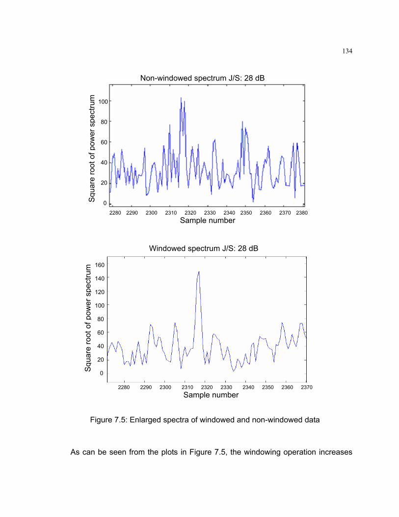
134
Figure 7.5: Enlarged spectra of windowed and non-windowed data
As can be seen from the plots in Figure 7.5, the windowing operation increases
Squa
re ro
ot o
f pow
er s
pect
rum
2280 2290 2300 2310 2320 2330 2340 2350 2360 2370 2380 Sample number
100 80 60 40 20 0 Sq
uare
root
of p
ower
spe
ctru
m
Non-windowed spectrum J/S: 28 dB
2280 2290 2300 2310 2320 2330 2340 2350 2360 2370 Sample number
Windowed spectrum J/S: 28 dB 160 140 120 100 80 60 40 20 0

135
the concentration of the interference frequency and reduces the number of
frequency bins that need to be excised. Windowing reduces the amount of
spectrum that must be excised, thus preserving more of the desired signal
spectrum. As a result, less signal energy loss and less distortion in the correlation
peak improve the accuracy of the position estimation and increase the maximum
tolerance of the interference mitigation algorithm. The plots in Figure 7.6 show the
effect of windowing on position estimation.

136
Figure 7.6: Effect of windowing on GPS position estimation.
135075 135080 135085 135089 135094 135099 135104 1351090
2
4
6
8
10
12
14
16
13:31 13:31 13:31 13:31 13:32 13:32 13:32 13:32
GPS Time(s); Local Time(hh:mm)
Pos
ition
erro
r (m
)
J/S =21 dB V = 80 m/s cold start with mitigation (with data window)
Horizontal error RMS = 5.44 (m) Vertical error RMS = 3.69 (m) Number of Sats: 7
135075 135080 135085 135089 135094 135099 135104 1351090
2
4
6
8
10
12
14
16
13:31 13:31 13:31 13:31 13:32 13:32 13:32 13:32
GPS Time(s); Local Time(hh:mm)
Pos
ition
erro
r (m
)
J/S =21 dB V = 80 m/s cold start with mitigation (no windows)
Horizontal error RMS = 5.59 (m) Vertical error RMS = 4.89 (m) Number of Sats: 6

137
The test was carried out in kinematic mode. The speed of the vehicle was set to
80 m/s under a J/S of 21 dB and in a cold start environment. From the GPS
position results, using a windowing operation, the position error root mean square
shows a slight improvement. Vertical error RMS decreased from 4.9 m to 3.7 m
and the horizontal RMS error decreased slightly from 5.6 m to 5.4 m. The number
of satellites that can be tracked increased from six to seven, which means that
employing a windowing operation allows all of the simulated satellites to be
tracked.
The addition of tracked satellites may not entail a commensurate improvement of
reliability because, if the pseudorange of the additional satellite has a large error
and it is used in least squares estimation, this satellite may deteriorate the
estimation result. In order to analyze the performance of the additional satellite,
the pseudorange errors of all the satellites are given in Figure 7.7. From this figure,
the reliability of the satellites can be analyzed.

138
Figure 7.7: Pseudorange error comparison between “with window” and “without window”

139
Only with the use of a windowing operation can satellite 16 be tracked. As it can
be seen in Figure 7.7, the pseudorange error of PRN 16 is at the same scale as
other satellites, which means that the measurement of this additional satellite is
reliable. By employing windowing, a greater number of satellites can be effectively
tracked and higher sensitivity can be achieved.
The above result came from a one-time test. In order to guarantee the stability of
this result, the test was carried out six times to produce a stochastically reliable
result. Under each J/S condition, the test was repeated six times. The results are
shown in Figure 7.8 and 7.9.
1 2 3 4 5 60
5
10
15
20
25
30
posi
tion
erro
r RM
S (m
)
Test number
Stochastic repeatability test
Horizontal error RMS mean = 15.34 (m) Vertical error RMS mean = 9.90 (m) J/S = 23 dB static test cold start with data window
Figure 7.8: Position errors of stochastic repeatability test with windowing

140
18 19 20 21 22 23 24 250
10
20
30
40
50
60
70
80
90
100
Suc
essf
ul ra
te (%
)
J/S (dB)
Rate of sucessful position fixing cold start
no data windowwith data window
Figure 7.9: Success rate of stochastic repeatability test with windowing
When J/S is below 23 dB, the position error is within 10 metres in all of the six
tests. If J/S increases to 23 dB, the position error increases also. The position
error varies for different samples due to the random noise. In some test samples,
the RMS error can reach 20 metres; however, the success rate in terms of
obtaining reasonable position solutions is still 100 percent with the window
operation. Thus, the interference mitigation algorithm of the data window,
combined with frequency excision, is statistically stable when J/S no greater than
23 dB.

141
When J/S increases to 24 and 25 dB, even with a windowing operation, the
successful rate of obtaining satisfactory position solutions is reduced to 16.7
percent, which means that only one out of 6 tests can achieve a solution. Under
this circumstance, the mitigation result is not stochastically repeatable. The
maximum tolerance of this mitigation algorithm with a data window is 23 dB under
cold start conditions. If the J/S is greater than 25 dB, a position cannot be
obtained.
From the above analysis of test results, the advantage of using a data window
before FFT transform is apparent. Although the improvement in position accuracy
is slight, the sensitivity has been improved, since more satellites can be effectively
tracked. Use of a data window, combined with the frequency excision algorithm,
can successfully mitigate interference of J/S values no greater than 23 dB under
cold start conditions. The maximum tolerance increases by 2 dB, as compared to
a traditional frequency excision algorithm, thus improving the sensitivity.

142
CHAPTER 8
Conclusions and Recommendations for Future Work
8.1 Conclusions
A RFI mitigation algorithm based on spectral analysis has been developed in this
thesis. The strategies of using an adaptive threshold for interference detection
and bit synchronization and using improved acquisition based on earlier
information were used to improve the mitigation results. The effectiveness of this
algorithm for CW, AM and FM interference has been investigated in acquisition,
tracking and position domain with the help of a software GPS receiver, a
hardware simulator and a signal generator. The influence of coherent integration
time, tracking loop bandwidth and integration time in the loop filter on the
mitigation results has also been investigated. The advantages of using windowing
and overlap processing before FFT are discussed and implemented in the
mitigation algorithm. Different sampling rates were used during the data collection
and the results of using different sampling rates have been compared and
analyzed.
143
Based on the results and findings obtained from the above results, the following
specific conclusions can be drawn:
1. The frequency excision algorithm is effective in mitigating a certain power level
of narrow-band RFI. An adaptive detection threshold that is a function of the
standard deviation of the normalized spectrum and the correlator power output
has better mitigation performance than the fixed detection threshold which is
suggested in the literature. The scalar factor in this function is determined
empirically and changes with different kinds of interference.
2. To obtain optimal mitigation results, this mitigation algorithm should combine
with some degree of control on software receiver parameters. For example,
adaptive selection of the following parameters may prove useful: coherent
integration time; tracking loop bandwidth; and integration time in the loop filter
for different interference levels and receiver dynamics.
3. The maximum tolerance of this algorithm in acquisition is a J/S of 28 dB with a
7 MHz sampling rate and a 20 ms coherent integration time. It produces a 3 dB
increase compared with a 4.75 MHz sampling rate whereas, in tracking, the
maximum tolerance entails a J/S of 30 dB at a 4.75 MHz sampling rate and 35
dB at a 7 MHz sampling rate.

144
4. In the position domain, for CW interference, no improvement was observed
with use of the mitigation algorithm in a warm start environment. In a cold start
environment, a stochastic repeatability test shows that the maximum J/S is 21
dB to achieve a 100 percent success rate in position fixing with use of the
mitigation algorithm. Without the mitigation algorithm, due to the inherent
anti-jamming property of the spread spectrum system, the J/S can reach a
maximum level of 18 dB.
5. In high dynamic mode (with a velocity of 80 m/s), by employing a soft
threshold in bit synchronization and improved acquisition based on a
combination of earlier information and a carefully chosen value for integration
time in the loop filter, the maximum mitigation ability for position fixing can
reach 21 dB in a cold start environment, the same level as in static mode.
6. This mitigation algorithm also effectively deals with AM and FM interference,
but the maximum tolerance is less than that found in the case of CW
interference. Also, FM interference causes more of a problem than AM
interference on this mitigation algorithm. In medium level modulation and cold
start conditions, the maximum tolerance for AM interference with mitigation
was observed at a J/S of 21 dB, which represents a 6 dB improvement as
compared to no mitigation algorithm. Whereas, for FM interference, the
maximum tolerance is 20 dB, a 5 dB improvement was observed as compared

145
to no mitigation algorithm.
7. Windowing and overlap processing before FFT transform has proven to be an
effective strategy to improve the performance of the frequency excision
algorithm. Although the improvement in position accuracy is slight, a larger
number of satellites can be effectively tracked. Thus, sensitivity is improved. A
data window combined with a frequency excision algorithm can successfully
mitigate interference of J/S values no greater than 23 dB in cold start
conditions, a 2 dB improvement as compared to a conventional frequency
excision algorithm.
8.2 Recommendations for future work
All of the tests conducted in this thesis are based on 1-bit analog-to-digital (A/D)
conversion. The 1-bit A/D converter is widely used in commercial GPS receivers.
However, in applications where RF interference may become a problem, a 1-bit
A/D converter is highly vulnerable to being captured by a CW jammer. For RFI
mitigation, the amount of narrow-band RF interference suppression is related to
the number of effective bits of A/D conversion precision that can be achieved at
IF.
Based on the above analysis, it is recommended, firstly, that future research be
undertaken to investigate the impact of the quantization bit on the mitigation

146
algorithm and the selection of the appropriate bit of quantization. There exists the
trade-off between computational burden and anti-jamming performance. Due to
the limited control provided by the Signal Tap, the software Global Navigation
Satellite System (GNSS) simulator developed by the University of Calgary’s PLAN
group may be a useful tool for this research.
The interference data set used in this thesis is simulated; thus, the interference
type is known before the mitigation algorithm is applied. However, in practical
applications, no prior knowledge is known about the interference. The second
recommendation for future research is to develop an algorithm to distinguish the
interference types and to develop a strategy for applying the various interference
detection thresholds.

147
References Accord Software & Systems Private Limited (2003). GPS Signal Tap Users Guide version 1.1. Bangalore, India. pp. 1-1. Badke, B. and Spanias, A.S. (2002). Partial band interference excision for GPS using frequency-domain exponents. Acoustics, Speech, and Signal Processing, 2002. Proceedings (ICASSP '02). IEEE International Conference on, Volume: 4, 13-17 May 2002, Pages: 3936 – 3939. Capozza, P.T., Holland, B. J., Li, C., Moulin, D., Pacheco, P., Rifkin, R. (1999), Measured effects of a narrowband interference suppressor on GPS receivers, In Proceedings of 55th annual meeting of the Institute of Navigation, June 1999, Cambridge, MA, Pages: 645 – 651. Capozza, P.T., Holland, B. J., Hopkinson, T. M., Landrau, R. L.(2000), A single-chip narrow-band frequency-domain excisor for the global positioning system (GPS) receiver, Solid-State Circuits, IEEE Journal of , Volume: 35 , Issue: 3 , March 2000, Pages: 401 – 411. Cooley, J.W. and Tukey, J.W. (1965) An algorithm for the machine calculation of complex Fourier series, Math. Comput. 19, Pages: 297–301. Cutright, C., Burns, J. R., Braasch, M. (2003). Characterization of Narrow-band interference mitigation performance versus quantization error in software radios. In Proceedings of 59th annual meeting of the Institute of Navigation, June 2003, Pages: 323–332. Deshpande, S., Cannon, M.E. (2004). Interference Effects on the GPS Signal Acquisition, National Technical Meeting, Institute of Navigation, 26-28 January, 2004, Pages: 1026 – 1037. Dipietro, R.C (1989). An FFT-based Technique for Suppressing Narrow-Band Interference, in PN Spread Spectrum Communications Systems. Acoustics, Speech, and Signal Processing, 1989. ICASSP-89., 1989 International Conference on, 23-26 May 1989, Pages:1360 - 1363 vol.2 Dong, L. (2003), IF GPS Signal Simulator Development and Verification, MSc. thesis, UCGE reports 20184, the University of Calgary

148
Harris, F. J.(1978) On the Use of Windows for Harmonic Analysis with the Discrete Fourier Transform. Proceedings of the IEEE. Vol. 66, January 1978, pp. 51-84. Heppe, S. (2002). GPS and GNSS RFI & Jamming Concerns I. ION GPS-2002 Tutorial, Portland, Oregon, pp. 45 Kaplan, E. (1996). GPS Satellite Signal Characteristics, Understanding GPS Signal Characteristics. Artech House, Inc., 685 Canton Street, Norwood, MA 0206. Krumvieda, K., Madhani, P., Cloman, C., Olson, E., Thomas, J., Axelrad, P., Kober, W. (2001), A complete IF Software GPS Receiver: A tutorial about the Details, ION GPS 2001, 11-14 September, 2001, Salt Lake City, UT, Pages: 789 – 811. Li, L. and Milstein, L. (1982), Adaptive Algorithms for Estimating and Suppressing Narrow-Band Interference in PN Spread-Spectrum Systems, Communications, IEEE Transactions on [legacy, pre - 1988], Volume: 30, Issue: 5, May 1982, Pages: 913 – 924. Lin, D.M., Tsui, J. (2000), Comparison of acquisition methods for software GPS receiver, Proceeding of ION GPS 2000, 19-22 September, 2000, Salt Lake City, UT, Pages: 2385 – 2390. Ma, C., G. Lachapelle, and M.E. Cannon (2004) Implementation of a Software GPS Receiver. Proceedings of GNSS 2004, Institute of Navigation, Long Beach, CA. September 21-24. MacGougan, G.D. (2003), High Sensitivity GPS Performance Analysis in Degraded Signal Environments, M.sc. thesis, UCGE reports 20176, the University of Calgary Ndili and Per Enge (1997). Receiver autonomous interference detection. In Proceedings of 53rd annual meeting of the Institute of Navigation, June 1997 Albuquerque, New Mexico, Pages: 79 – 88. Oppenheim, A.V., and Schafer, R.W. (1989). Discrete-Time Signal Processing. Prentice-Hall, 1989, pp. 447-448. Parkinson, B. and Spilker, J. J. (1996). Global Positioning System: Theory And Applications Volume 1. American Institute of Aeronautics and Astronautics, Inc.,

149
Peterson, B., Hartnett, J., Fiedler, R., Nebrich, A. (1996). Frequency Domain Techniques for fast GPS acquisition and interference detection/rejection. Navigation: Journal of the institute of navigation, Vol.43, No. 3, Fall 1996. Proakis, J.G and Ketchum, J.W. (1982). Adaptive Algorithms for Estimating and Suppressing Narrow-Band Interference in PN Spread-Spectrum Systems COM-30 (May 1982), IEEE Trans. Communications, Volume: 30, Issue: 5, Pages:913 – 924. Proakis, J.G. (1996a). Digital signal processing: principles, algorithms, and applications. Prentice-Hall, Inc., Upper Saddle River, New Jersey 07458, pp. 243. Proakis, J.G. (1996b). Interference suppression in spread spectrum systems. Spread Spectrum Techniques and Applications Proceedings, 1996, IEEE 4th International Symposium on, Volume: 1, 22-25 Sept. 1996, pp.259 – 266. Przyjemski, J., E. Balboni, and J. Dowdle. (1993). GPS anti-jam enhancement techniques. Proc. ION 49th annual meeting, Cambridge, MA, June 1993, pp. 41-50. Raquet, J.F. (2004), Engo 699.10 Lecture note: GPS receiver design, Department of Geomatics Engineering, The University of Calgary. Rash, G. D. (1997). GPS Jamming In A Laboratory Environment. In Proceedings of the Institute of Navigation ION GPS-97 (September 16-19, 1997, Kansas City, Missouri), pp. 389–398. Ray, J.K. (2003), ENGO 699.73 Lecture note: Advanced GPS Receiver Technology, Department of Geomatics Engineering, The University of Calgary. Rifkin, R. and Vaccaro, J.J.(2000). Comparison of narrowband adaptive filter technologies for GPS. Position Location and Navigation Symposium, IEEE 2000 , 13-16 March 2000. Pages:125 – 131. Spirent communications limited (2003a). SimGEN (Including SimLOCATE) user manual. Software for the Spirent range of satellite navigation simulator products Spirent communications limited (2003b). User manual for the GSS 4765 interference simulation system operation with SimGEN for windows. Tsui, James B-Y. (2000). Fundamentals of Global Positioning System Receivers: A Software Approach, John Wiley & Sons Inc.
150
Tukey, J. W. and Cooley, J. W. (1966). An algorithm for the machine calculation of complex Fourier series, Math. Comput. 19, 297–301 (1965). Van Nee, R.D.J., COENEN, A.J.R.M. (1991). New Fast GPS Code-Acquisition Technique using FFT, Electronic Letters, Vol. 27, pp.158 -160, Jan. 1991. Wang, C. and Amin, M.G. (1998). Performance analysis of instantaneous frequency-based interference excision techniques in spread spectrum communications. Signal Processing, IEEE Transactions on Volume: 46, Issue: 1, Jan. 1998, Pages: 70 – 82. Ward, P. (1996). Satellite signal acquisition and tracking, in Understanding GPS: Principles and applications, Elliott Kaplan (ED.), Artech House. Ward, P.W. (2002). GPS and GNSS RFI & Jamming Concerns III. ION GPS-2002 Tutorial, Portland, Oregon, pp. 8-24. Young, J. A. and Lehnert, J. S. (1994), Sensitivity loss of real-time DFT-based frequency excision with direct sequence spread-spectrum communication, Tactical Communications Conference, 1994. Vol.1. Digital Technology for the Tactical Communicator, Proceedings of the 1994, 10-12 May 1994, Pages: 409 - 420