Embed Size (px)
Citation preview
University of Kentucky University of Kentucky
UKnowledge UKnowledge
University of Kentucky Master's Theses Graduate School
2008
Thevenin Equivalent Circuit Estimation and Application for Power Thevenin Equivalent Circuit Estimation and Application for Power
System Monitoring and Protection System Monitoring and Protection
Mohammad M. Iftakhar University of Kentucky
Right click to open a feedback form in a new tab to let us know how this document benefits you. Right click to open a feedback form in a new tab to let us know how this document benefits you.
Recommended Citation Recommended Citation Iftakhar, Mohammad M., "Thevenin Equivalent Circuit Estimation and Application for Power System Monitoring and Protection" (2008). University of Kentucky Master's Theses. 583. https://uknowledge.uky.edu/gradschool_theses/583
This Thesis is brought to you for free and open access by the Graduate School at UKnowledge. It has been accepted for inclusion in University of Kentucky Master's Theses by an authorized administrator of UKnowledge. For more information, please contact [email protected].

ABSTRACT OF THESIS
Thevenin Equivalent Circuit Estimation and Application for Power System Monitoring and Protection
The Estimation of Thevenin Equivalent Parameters is useful for System Monitoring and Protection. We studied a method for estimating the Thevenin equivalent circuits. We then studied two applications including voltage stability and fault location. A study of the concepts of Voltage Stability is done in the initial part of this thesis. A Six Bus Power System Model was simulated using MATLAB SIMULINK®. Subsequently, the Thevenin Parameters were calculated. The results were then used for two purposes, to calculate the Maximum Power that can be delivered and for Fault Location. KEYWORDS: Thevenin Equivalent Circuit, Voltage Stability, Rotor Angle Stability, Fault Location, Power System Monitoring Mohammad M Iftakhar
December 31st 2008

Thevenin Equivalent Circuit Estimation and Application for Power System Monitoring and Protection
By
Mohammad Museb Iftakhar
____________________________________
(Director of Thesis)
____________________________________
(Director of Graduate Studies)
____________________________________
(Date)

RULES FOR THE USE OF THESIS
Unpublished thesis submitted for the Master’s degree and deposited in the University of
Kentucky Library are as a rule open for inspection, but are to be used only with due
regard to the rights of the authors. Bibliographical references may be noted, but
quotations or summaries of parts may be published only with the permission of the
author, and with the usual scholarly acknowledgments.
Extensive copying or publication of the dissertation in whole or in part also requires the
consent of the Dean of the Graduate School of the University of Kentucky.
A library that borrows this dissertation for use by its patrons is expected to secure the
signature of each user.
Name
________________________________________________________________________________________________________________________________________________________________________________________________________________________________________________________________________________________________________________________________________________________________________________________________________________________________________________________________________________________________________________________________________________________________________________________________________________________________________________________________________________________________________________________________________________
Date ________________________________________________________________________ ________________________________________________________________________ ________________________________________________________________________ ________________________________________________________________________ ________________________________________________________________________ ________________________________________________________________________ ________________________________________________________________________

THESIS
Mohammad Museb Iftakhar
The Graduate School
University of Kentucky
2009
Thevenin Equivalent Circuit Estimation and Application for Power System Monitoring
and Protection
THESIS
A thesis submitted in partial fulfillment of the requirements for the degree of Master
of Science in the College of Engineering at the
University of Kentucky
By
Mohammad Museb Iftakhar
Lexington, Kentucky
Director: Dr. Yuan Liao, Department of Electrical and Computer Engineering
Lexington, Kentucky
2009
Copyright © Mohammad Museb Iftakhar 2009

Dedicated to My Parents, Brothers and Sister

iii
ACKNOWLEDGEMENTS
I would like to take this opportunity to express my sincere thanks and heartfelt gratitude
to my academic advisor and thesis chair Dr. Yuan Liao for his guidance and support
throughout my thesis. I am very thankful for his constant encouragement during the
thesis. Without him the thesis would have never taken its present shape. I am greatly
indebted for his support.
My parents and my siblings have been great sources of support throughout my studies.
My friends have given me a lot of love without which this work would not have been
possible.
I also would like to extend my thanks to Dr. Paul A Dolloff and Dr. Jimmy J Cathey for
serving on my thesis committee and providing me with invaluable comments and
suggestions for improving this thesis.

iv
Table of Contents
ACKNOWLEDGEMENTS .............................................................................................. III
LIST OF TABLES ............................................................................................................ VI
LIST OF FIGURES ......................................................................................................... VII
1. INTRODUCTION .......................................................................................................... 1
1.1 BACKGROUND ..................................................................................................... 11.2 PURPOSE OF THE THESIS ...................................................................................... 21.3 OVERVIEW OF SYSTEM STABILITY ....................................................................... 21.4 EQUATION OF MOTION OF A ROTATING MACHINE ............................................... 31.5 STEADY STATE STABILITY ................................................................................... 41.6 METHODS OF IMPROVING STEADY STATE STABILITY LIMIT ................................. 71.7 TRANSIENT STABILITY LIMIT ............................................................................... 81.8 EQUAL AREA CRITERION ..................................................................................... 81.9 FACTORS AFFECTING TRANSIENT STABILITY ...................................................... 9
2. POWER SYSTEM VOLTAGE STABILITY ANALYSIS ......................................... 11
2.1 DEFINITION AND CLASSIFICATION OF POWER SYSTEM STABILITY ..................... 112.2 CLASSIFICATION OF POWER SYSTEM STABILITY ................................................ 112.3 VOLTAGE STABILITY ......................................................................................... 122.4 VOLTAGE STABILITY ANALYSIS ........................................................................ 122.5 P-V CURVES ...................................................................................................... 162.6 V-Q CHARACTERISTICS ..................................................................................... 172.7 SOME SIGNIFICANT RESULTS AND CRITERIA IN VOLTAGE STABILITY ............... 19
3. POWER SYSTEM MODELING AND THEVENIN EQUIVALENT CIRCUIT PARAMETERS ESTIMATION ....................................................................................... 21
3.1 TRANSMISSION LINE DATA ................................................................................ 213.2 GENERATOR DATA ............................................................................................. 223.3 LOAD DATA ....................................................................................................... 233.4 ALGORITHM FOR THEVENIN EQUIVALENT CIRCUIT ESTIMATION ...................... 233.5 EQUATION FOR MAXIMUM POWER DELIVERED ................................................. 273.6 VOLTAGE AND CURRENT WAVEFORMS AT LOAD BUS L3 .................................. 293.7 WAVEFORMS FOR VOLTAGE AND CURRENT AT THE LOAD BUS L5 .................... 35
4. FAULT ANALYSIS AND ESTIMATION OF FAULT LOCATION ........................ 41
4.1 UNSYMMETRICAL FAULTS ................................................................................. 414.2 SYMMETRICAL COMPONENT ANALYSIS OF UNSYMMETRICAL FAULTS .............. 414.3 ANALYSIS OF SINGLE LINE TO GROUND FAULT ................................................. 454.4 ANALYSIS OF LINE TO LINE FAULT .................................................................... 474.5 DOUBLE LINE TO GROUND FAULT ANALYSIS .................................................... 504.6 FAULT LOCATION ALGORITHM .......................................................................... 52

v
4.7 IMPEDANCE BASED ALGORITHM ...................................................................... 534.8 VOLTAGE AND CURRENT WAVEFORMS FOR DIFFERENT FAULT LOCATIONS .... 55
5. CONCLUSION ............................................................................................................. 59
BIBLIOGRAPHY ............................................................................................................. 60
VITA ................................................................................................................................. 62
vi
List of Tables
TABLE 3.1 GENERATORS BLOCK PARAMETER VALUES ..................................................... 22TABLE 3.2 LOAD BLOCK PARAMETER VALUES ................................................................. 23TABLE 3.3 VOLTAGE AND CURRENTS AT BUS L3 .............................................................. 25TABLE 3.4 VOLTAGE AND CURRENT AT LOAD BUS L5 ...................................................... 26TABLE 3.5 THEVENIN PARAMETERS FOR 4, 5 AND 6 SETS OF MEASUREMENTS AT LOAD BUS
L3 .............................................................................................................................. 26TABLE 3.6 THEVENIN PARAMETERS FOR 4, 5 AND 6 SETS OF MEASUREMENTS AT LOAD BUS
L5 .............................................................................................................................. 27TABLE 3.7 POWER DELIVERED AT THE BUS L3 FOR DIFFERENT POWER FACTOR ANGLES . 28TABLE 3.8 POWER DELIVERED AT THE BUS L5 FOR DIFFERENT POWER FACTOR ANGLES . 28TABLE 4.1 FAULT LOCATION ESTIMATION ......................................................................... 54

vii
List of Figures
FIGURE 1.1 MACHINE CONNECTED TO INFINITE BUS ........................................................... 5FIGURE 1.2 POWER ANGLE CURVE ...................................................................................... 6FIGURE 1.3 CURVE SHOWING THE EQUAL AREA CRITERION ................................................ 9FIGURE 2.1 SIMPLE RADIAL SYSTEM FOR VOLTAGE STABILITY ANALYSIS ........................ 13FIGURE 2.2 REACTIVE END VOLTAGES, POWER AND CURRENT AS A FUNCTION OF LOAD
DEMAND .................................................................................................................... 15FIGURE 2.3 POWER VOLTAGE CHARACTERISTICS FOR THE SYSTEM OF FIGURE2.1 ............ 16FIGURE 2.4 POWER VOLTAGE CHARACTERISTICS FOR DIFFERENT LOAD POWER FACTORS 17FIGURE 2.5 SIMPLE RADIAL TWO BUS SYSTEM ................................................................. 18FIGURE 2.6 V-Q CHARACTERISTICS OF THE SYSTEM IN FIGURE 2.1 ................................... 18FIGURE 3.1 SIX BUS POWER SYSTEM MODEL .................................................................... 21FIGURE 3.2 THEVENIN EQUIVALENT CIRCUIT .................................................................... 24FIGURE 3.3 EQUIVALENT POWER SYSTEM MODEL FOR CALCULATING MAXIMUM POWER
DELIVERED ................................................................................................................ 28FIGURE 3.4(A) VOLTAGE SIGNALS FOR THE CASE WITH GENERATOR 2 ANGLES SET TO 10
DEGREES. ................................................................................................................... 29FIGURE 3.4(B) CURRENT SIGNALS FOR THE CASE WITH GENERATOR 2 ANGLES SET TO 10
DEGREES. ................................................................................................................... 29FIGURE 3.5(A) VOLTAGE SIGNALS FOR THE CASE WITH GENERATOR 2 ANGLES SET TO 20
DEGREES .................................................................................................................... 30FIGURE 3.5(B) CURRENT SIGNALS FOR THE CASE WITH GENERATOR 2 ANGLES SET TO 20
DEGREES .................................................................................................................... 30FIGURE 3.6(A) VOLTAGE SIGNALS FOR THE CASE WITH GENERATOR 2 ANGLES SET TO 30
DEGREES .................................................................................................................... 31FIGURE 3.6(B) CURRENT SIGNALS FOR THE CASE WITH GENERATOR 2 ANGLES SET TO 30
DEGREES .................................................................................................................... 31FIGURE 3.7(A) VOLTAGE SIGNALS FOR THE CASE WITH GENERATOR 2 ANGLES SET TO 40
DEGREES .................................................................................................................... 32FIGURE 3.7(B) CURRENT SIGNALS FOR THE CASE WITH GENERATOR 2 ANGLES SET TO 40
DEGREES .................................................................................................................... 32FIGURE 3.8(A) VOLTAGE SIGNALS FOR THE CASE WITH GENERATOR 2 ANGLES SET TO 60
DEGREES .................................................................................................................... 33FIGURE 3.8(B) CURRENT SIGNALS FOR THE CASE WITH GENERATOR 2 ANGLES SET TO 60
DEGREES .................................................................................................................... 33FIGURE 3.9(A) VOLTAGE SIGNALS FOR THE CASE WITH GENERATOR 2 ANGLES SET TO 0
DEGREES .................................................................................................................... 34FIGURE 3.9(B) CURRENT SIGNALS FOR THE CASE WITH GENERATOR 2 ANGLES SET TO 0
DEGREES .................................................................................................................... 34FIGURE 3.10(A) VOLTAGE SIGNALS FOR THE CASE WITH GENERATOR 3 ANGLES SET TO 0
DEGREES .................................................................................................................... 35FIGURE 3.10(B) CURRENT SIGNALS FOR THE CASE WITH GENERATOR 3 ANGLES SET TO 0
DEGREES .................................................................................................................... 35

viii
FIGURE 3.11(A) VOLTAGE SIGNALS FOR THE CASE WITH GENERATOR 3 ANGLES SET TO 10 DEGREES .................................................................................................................... 36
FIGURE 3.11(B) CURRENT SIGNALS FOR THE CASE WITH GENERATOR 3 ANGLES SET TO 10 DEGREES .................................................................................................................... 36
FIGURE 3.12(A) VOLTAGE SIGNALS FOR THE CASE WITH GENERATOR 3 ANGLES SET TO 20 DEGREES .................................................................................................................... 37
FIGURE 3.12(B) CURRENT SIGNALS FOR THE CASE WITH GENERATOR 3 ANGLES SET TO 20 DEGREES .................................................................................................................... 37
FIGURE 3.13(A) VOLTAGE SIGNALS FOR THE CASE WITH GENERATOR 3 ANGLES SET TO 30 DEGREES .................................................................................................................... 38
FIGURE 3.13(B) CURRENT SIGNALS FOR THE CASE WITH GENERATOR 3 ANGLES SET TO 30 DEGREES .................................................................................................................... 38
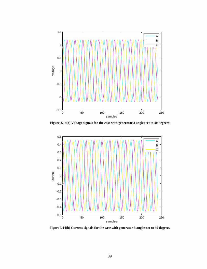
FIGURE 3.14(A) VOLTAGE SIGNALS FOR THE CASE WITH GENERATOR 3 ANGLES SET TO 40 DEGREES .................................................................................................................... 39
FIGURE 3.14(B) CURRENT SIGNALS FOR THE CASE WITH GENERATOR 3 ANGLES SET TO 40 DEGREES .................................................................................................................... 39
FIGURE 3.15(A) VOLTAGE SIGNALS FOR THE CASE WITH GENERATOR 3 ANGLES SET TO 60 DEGREES .................................................................................................................... 40
FIGURE 3.15(B) CURRENT SIGNALS FOR THE CASE WITH GENERATOR 3 ANGLES SET TO 60 DEGREES .................................................................................................................... 40
FIGURE 4.1 A GENERAL POWER NETWORK ....................................................................... 42FIGURE 4.2 (A) POSITIVE SEQUENCE NETWORK AS SEEN FROM THE FAULT POINT .............. 42FIGURE 4.2 (B) NEGATIVE SEQUENCE NETWORK AS SEEN FROM THE FAULT POINT ........... 43FIGURE 4.2(C) ZERO SEQUENCE NETWORK AS SEEN FROM THE FAULT POINT ..................... 43FIGURE 4.2 (D) THEVENIN EQUIVALENT OF POSITIVE SEQUENCE NETWORK AS SEEN FROM F
................................................................................................................................... 43FIGURE 4.2 (E) THEVENIN EQUIVALENT OF NEGATIVE SEQUENCE NETWORK AS SEEN FROM
F ................................................................................................................................ 44FIGURE 4.2 (F) THEVENIN EQUIVALENT OF ZERO SEQUENCE NETWORK AS SEEN FROM F . 44FIGURE 4.3(A) SINGLE LINE TO GROUND FAULT AT F ....................................................... 45FIGURE 4.3(B) CONNECTION OF SEQUENCE NETWORKS FOR SINGLE LINE TO GROUND FAULT
................................................................................................................................... 47FIGURE 4.4(A) LINE TO LINE FAULT THROUGH IMPEDANCE fZ ......................................... 48 FIGURE 4.4(B) POSITIVE AND NEGATIVE SEQUENCE CONNECTIONS FOR A LINE TO LINE
FAULT ........................................................................................................................ 49FIGURE 4.4(C) THEVENIN EQUIVALENT FOR CONNECTION OF SEQUENCE NETWORKS FOR L-
L FAULT ..................................................................................................................... 50FIGURE 4.5(A) DOUBLE LINE TO GROUND FAULT THROUGH IMPEDANCE fZ .................... 51 FIGURE 4.5(B) CONNECTION OF SEQUENCE NETWORKS FOR A DOUBLE LINE TO GROUND
FAULT ........................................................................................................................ 52FIGURE 4.5(C) THEVENIN EQUIVALENT FOR THE SEQUENCE NETWORK CONNECTIONS FOR A
LLG FAULT ................................................................................................................ 52FIGURE 4.6 TRANSMISSION LINE CONSIDERED FOR THE ALGORITHM [5] .......................... 53FIGURE 4.7 NEGATIVE SEQUENCE NETWORK DURING THE FAULT NEGLECTING SHUNT
CAPACITANCE [5] ....................................................................................................... 53

ix
FIGURE 4.8(A) VOLTAGE WAVEFORMS FOR A PHASE A TO GROUND FAULT WITH A FAULT LOCATION OF 0.2 P.U .................................................................................................. 55
FIGURE 4.8(B) CURRENT WAVEFORMS FOR A PHASE A TO GROUND FAULT WITH A FAULT LOCATION OF 0.2 P.U .................................................................................................. 55
FIGURE 4.9(A) VOLTAGE WAVEFORMS FOR A PHASE A TO GROUND FAULT WITH A FAULT LOCATION OF 0.4 P.U .................................................................................................. 56
FIGURE 4.9(B) CURRENT WAVEFORMS FOR A PHASE A TO GROUND FAULT WITH A FAULT LOCATION OF 0.4 P.U .................................................................................................. 56
FIGURE 4.10(A) VOLTAGE WAVEFORMS FOR A PHASE A TO GROUND FAULT WITH A FAULT LOCATION OF 0.6 P.U .................................................................................................. 57
FIGURE 4.10(B) CURRENT WAVEFORMS FOR A PHASE A TO GROUND FAULT WITH A FAULT LOCATION OF 0.6 P.U .................................................................................................. 57
FIGURE 4.11(A) VOLTAGE WAVEFORMS FOR A PHASE A TO GROUND FAULT WITH A FAULT LOCATION OF 0.7 P.U .................................................................................................. 58
FIGURE 4.11(B) CURRENT WAVEFORMS FOR A PHASE A TO GROUND FAULT WITH A FAULT LOCATION OF 0.7 P.U .................................................................................................. 58
1
1. Introduction
1.1 Background
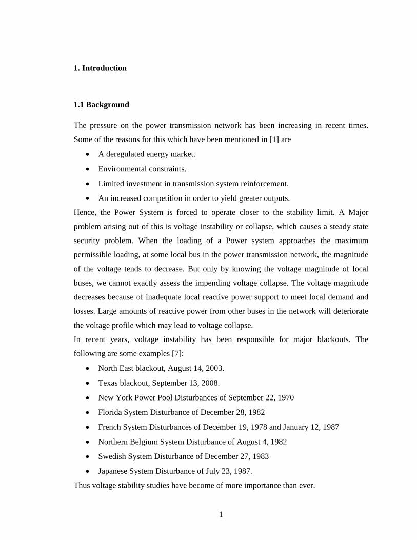
The pressure on the power transmission network has been increasing in recent times.
Some of the reasons for this which have been mentioned in [1] are • A deregulated energy market.
• Environmental constraints.
• Limited investment in transmission system reinforcement.
• An increased competition in order to yield greater outputs.
Hence, the Power System is forced to operate closer to the stability limit. A Major
problem arising out of this is voltage instability or collapse, which causes a steady state
security problem. When the loading of a Power system approaches the maximum
permissible loading, at some local bus in the power transmission network, the magnitude
of the voltage tends to decrease. But only by knowing the voltage magnitude of local
buses, we cannot exactly assess the impending voltage collapse. The voltage magnitude
decreases because of inadequate local reactive power support to meet local demand and
losses. Large amounts of reactive power from other buses in the network will deteriorate
the voltage profile which may lead to voltage collapse.
In recent years, voltage instability has been responsible for major blackouts. The
following are some examples [7]:
• North East blackout, August 14, 2003.
• Texas blackout, September 13, 2008.
• New York Power Pool Disturbances of September 22, 1970
• Florida System Disturbance of December 28, 1982
• French System Disturbances of December 19, 1978 and January 12, 1987
• Northern Belgium System Disturbance of August 4, 1982
• Swedish System Disturbance of December 27, 1983
• Japanese System Disturbance of July 23, 1987.
Thus voltage stability studies have become of more importance than ever.
2
Another important thing to consider in this thesis is fault location. Fault location studies
are very important for the transient stability limit of the system. The increased
complexities of modern power systems have raised the importance of fault location
research studies [11]. Accurate and fast fault location helps in reducing the maintenance
and restoration times, reduce the outage times and thus improve the power system
reliability [12].
1.2 Purpose of the Thesis
To operate the power system with an adequate security margin, it is essential to estimate
the maximum permissible loading [1].The maximum power that can be transferred to the
load bus in a power system can be effectively studied by estimating the Thevenin
equivalent circuit of the power system Model. Thus, in one part of my Thesis, I will be
calculating the Thevenin parameters of a six bus power system model. This would
provide me with considerable results to calculate the maximum power that can be
delivered. The Thevenin equivalent circuit parameters are useful in the applications for
power system monitoring and protection. The Thevenin parameters that I obtain in the
first part are used for fault location based on voltage measurements. The fault location
algorithm is taken from [5], which are described in detail in Chapter 4.
1.3 Overview of System Stability
The stability of a system of interconnected dynamic components is its ability to return to
normal or stable operation after having been subjected to some form of disturbance [8].
In a power system, we typically deal with two forms of instability: The loss of
synchronism between synchronous machines and voltage instability. Synchronous
stability can be classified as steady state and transient stability and are studied in this
chapter. The voltage stability is studied in the next chapter. The equations and figures in
the subsequent sections have mainly been obtained from [4] and [8].
As defined in [8], steady state stability is the ability of the power system, when operating
under given load conditions, to retain synchronism when subjected to small disturbances
3
such as the continual changes in load or generation and the switching out of lines. This is
also known as dynamic stability.
Transient stability deals with sudden and large changes in the system. One example is
faults in a Power system. During fault conditions, the stability limit is less than the steady
state condition. Before we make a detailed study of steady state and transient stability, it
is important to study the equation of motion of a rotating machine.
1.4 Equation of Motion of a Rotating Machine
In this section, we will be studying the Equation of Motion of a Rotating Machine and
deriving the swing equation. The equations in this section have all been obtained from
[8].
Let the moment of inertia of the rotor be I and the angular acceleration isα . T∆ is the
net torque applied on the rotor. ω is the synchronous speed of the rotor (radians/second).
The kinetic energy absorbed by the rotor is given by 2
21 ωI Joules.
The angular momentum is ωIM = Joules-Seconds per radian. An inertia constant, H can
be defined as the stored energy at synchronous speed per volt-ampere of the rating of the
machine [8]. As we know that the unit of energy used in power systems analysis is
Kilojoules or Mega joules and if we consider the rating of the machine to be G Mega-
Volt-Amperes, then by multiplying G with the inertia constant we get the kinetic energy
of the machine.
ωω MIGH21
21 2 == is the Kinetic Energy or the stored Energy. (1.1)
f360=ω Electrical Degrees per second where f is the system frequency in Hz. (1.2)
Substituting (1.2) in (1.1)
fMGH )360(21
= (1.3)
fGHM 180/=⇒ Mega joule-seconds/electrical degree (1.4)
=∆T Mechanical Torque Input- Electrical Torque Output
2
2
dtdI δ
= (1.5)

4
( )2/2 22
2
ωωωδ
xIT
IT
dtd ∆
=∆
=∴ (1.6)
..2.ExK
Pω∆= (1.7)
Here electricalmech PPP −=∆ (1.8)
By using Equation (1.1) in (1.7), we can write
MP
dtd ∆
=2
2δ (1.9)
There is an increase in the value of δ when there is a negative change in the Power
output in Equation (1.9). electricalmech PPP −=∆ is sometimes considered as the change in
Electrical Power output. An increase in electricalP∆ will increase the value ofδ . The Power
input is assumed to be constant.
MP
dtd ∆
−=⇒ 2
2δ or 02
2
=∆+ PdtdM δ (1.10)
Equation (1.10) is known as Swing Equation.
Now that we have studied about the Equation of Motion of Rotating Machine, we can
analyze Steady State and Transient Stability of a System based on this.
1.5 Steady State Stability
In this section we will be studying the steady state analysis for a power system. The
equations in this section have been obtained from [4]. The steady state stability limit of a
particular circuit of a power system is defined as the maximum power that can be
transmitted to the receiving end without loss of synchronism [4].Figure 1.1[4] represents
a simple system for the purpose of analysis.
The dynamics of this system are described by the equations (1.11) to (1.13)
em PPdtdM −=2
2δ (1.11)
fHMπ
= in the Per Unit System (1.12)

5
δδ sinsin maxPX
VEP
de == (1.13)
dX is the direct axis reactance . The plot for equation (1.13) also known as the power
angle curve is represented in Figure 1.2[4]
+
δ∠'E
dX 'eX
eP
00∠V
Infinite Bus
Figure 1.1 Machine Connected to Infinite Bus
The system has a steady power transfer meo PP = and the torque angle is oδ as shown in
Figure 1.2. For a small increment P∆ in the electric power with the input mP being
constant, the torque angle changes to ( )δδ ∆+o . Linearizing about the operating point
),( oeoo PQ δ [4], we get
δδ
∆
∂∂
=∆0
ee
PP (1.14)
Rewriting Equation (1.11) in the current analysis,
( ) eeeom PPPPdt
dM ∆−=∆+−=∆
2
2 δ (1.15)
Using Equation (1.14) in (1.15)
00
2
2
=∆
∂∂
+∆ δ
δδ eP
dtdM (1.16)
00
2 =∆
∂∂
+⇒ δδ
ePMk (1.17)

6
Where dtdk =
The stability of the system for small changes is determined by the characteristic equation
[4] 00
2 =
∂∂
+δ
ePMk (1.18)
The roots of Equation (1.18) are given by
( ) 21
0/
∂∂−±=
MP
k e δ (1.19)
eP
eeo PP ∆+ maxP
eoPoQ
oδδδ ∆+o
δ090 0180
0180− 090−
Generator
Motor
Figure 1.2 Power Angle Curve
Now the system behavior depends on the value of 0)/( δ∂∂ eP .
If 0)/( δ∂∂ eP is positive, the roots are imaginary and conjugate. The system behavior is
oscillatory about oδ . But in our analysis the machine damper windings line resistance had

7
been neglected. These cause the system oscillations to decay and hence the system is
stable for a small increment in power.
If 0)/( δ∂∂ eP is negative, the roots are real. One is positive and the other is negative.
Though, they are equal in magnitude. For a small increment in power, the system is
unstable as the synchronism is lost due to increase in torque angle with increase in power.
From Equation (1.13) assuming VE , to remain constant, the system is unstable
if 090>oδ . (1.20)
The maximum power transfer without loss of stability occurs for 090=oδ (1.21)
The maximum power transferred is therefore given by
XVE
P =max (1.22)
But in the analysis we had assumed that the internal machine voltage remains constant. In
such a case as the loading is increased, the terminal voltage dips heavily which is
practically not acceptable. In practice, we must consider the steady state stability limit by
assuming that the excitation is adjusted for every load increase to keep the terminal
voltage constant. The effects of governor and excitation control were not considered in
the analysis.
Steady state stability limit is very important as it should be taken care that a system can
operate above transient stability but not above steady state stability limit. The transient
stability limit can be made to closely approach the steady state limit currently with
increased speeds in fault clearing.
1.6 Methods of Improving Steady State stability Limit
The following methods can be used depending on the conditions in order to improve the
steady state stability limit [4]
• From Equation (1.22), we can say that the steady state stability limit can be
improved by reducing X or by increasing either E or V or both.
• For transmission lines of high reactance, the stability limit can be increased by
using two parallel lines.
8
• Use of series capacitors in the lines to get better voltage regulation raises the
stability limits by decreasing the line reactance.
• Employing quick excitation systems and higher excitation voltages.
1.7 Transient Stability Limit
Transient stability limit is the maximum possible power that can be transmitted through a
point in the system when the system is operating with stability during transient
disturbances [15]. The type of disturbance and the duration of disturbance affect the
transient stability limit. The duration of a fault determines the amount of power that can
be transmitted from one machine to another machine in a two machine system without
loss of synchronism. The power limit is determined using the Equal Area Criterion. This
is studied in section 1.8.
1.8 Equal Area Criterion
As we had considered one finite machine system for analysis for steady state stability, we
will study the Equal Area Criterion for one finite machine swinging with an infinite bus
in this section. The equations in this section have been mainly obtained from [15]. The
detailed study of Equal Area Criterion for a system with two finite machines swinging
with respect to each other is discussed in [4] and [15].
The Swing Equation of a finite machine swinging with respect to an infinite machine is
given by aem PPPdtdM =−=2
2δ (1.23)
Multiplying both sides of Equation (1.23) by dtd /2 δ and rearranging, we get
dtd
MP
dtd
dtd a δδδ 22 2
2
= (1.24)
dtd
MP
dtd
dtd a δδ 2
2
=
⇒ (1.25)
Upon integrating Equation (1.25) with respect to time, we get
9
∫=
δ
δ
δδ
o
dPMdt
da
22
(1.26)
∫==⇒δ
δ
δωδ
o
dPMdt
da
2 (1.27)
0=ω when the machine comes to rest with respect to the infinite machine. The
condition required for the stability of a single machine system connected to infinite bus is
0=∫δ
δ
δo
dPa (1.28)
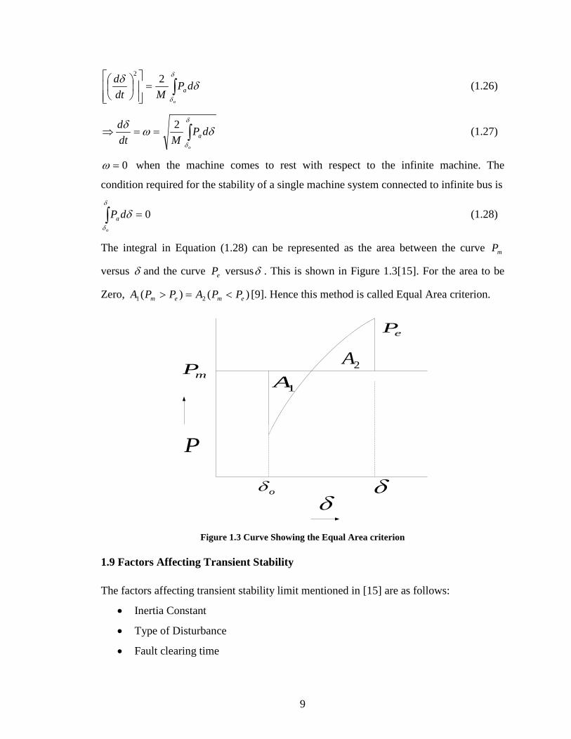
The integral in Equation (1.28) can be represented as the area between the curve mP
versus δ and the curve eP versusδ . This is shown in Figure 1.3[15]. For the area to be
Zero, )()( 21 emem PPAPPA <=> [9]. Hence this method is called Equal Area criterion.
δoδδ
mP
eP
P
1A2A
Figure 1.3 Curve Showing the Equal Area criterion
1.9 Factors Affecting Transient Stability
The factors affecting transient stability limit mentioned in [15] are as follows:
• Inertia Constant
• Type of Disturbance
• Fault clearing time

10
• Location of the fault
• Initial operating Condition of the system
• The way in which the fault is cleared.
Thus, in this chapter we have presented the purpose of the thesis research that has been
carried out and an overview of the basic concepts related to the area of my research. An
advanced study of these concepts can be made through the references that have been
mentioned.
11
2. Power System Voltage Stability Analysis
In chapter 1, I gave an overview about the importance of voltage stability studies as
voltage instability or voltage collapse may lead to a blackout. In this chapter we will be
making a detailed study of the relevant concepts that could help us make the
understanding of voltage stability better. Before we study voltage stability in particular,
we define and classify power system stability in general. This is studied in the initial
sections of this chapter. In the later sections we discuss voltage stability. These include
the definitions, concepts of mathematical formulation of the voltage stability problems
and some significant criteria of voltage stability studies. The equations and figures have
been mainly obtained from [2] and [4].
2.1 Definition and Classification of Power System stability
In a broad terminology, power system stability may be defined as that property of the
power system that enables it to remain in a state of operating equilibrium under normal
operating conditions and to regain an acceptable state of equilibrium after being subjected
to a disturbance [2]. The definitions of power system stability though have not been
precise and do not include all practical instability scenarios [3]. A proposal is presented
in [3] which attempts to define power system stability more precisely which includes all
forms of system instability. “Power system stability is the ability of an electric power
system, for a given initial operating condition, to regain a state of operating equilibrium
after being subjected to a physical disturbance with most system variables bounded so
that practically the entire system remains intact” [3].
2.2 Classification of Power System Stability
Power system stability is classified based on the following considerations [2]
• The physical nature of the instability
• The size of the disturbance
• The time span
12
Based on the physical nature of the instability, it can be classified as rotor angle stability
and voltage stability. Based on the size of the disturbance, it is classified as large
disturbance and small disturbance stability. Based on the time span, it can be classified as
long term and short term stability.
2.3 Voltage Stability
Voltage stability is the ability of a power system to maintain steady acceptable voltages at
all buses in the system under normal operating conditions and after being subjected to a
disturbance [2]. There is voltage instability when there is voltage drop in the system or at
a bus due to several reasons which include a general disturbance, a change in system
condition or due to fluctuating loads. But the main reason for a voltage instability is the
inadequacy of reactive power demands to be met by the system.
Reactive power is injected into the system to meet the increasing demands. For a voltage
stable system, as the reactive power is injected into the buses in the system, the voltage
magnitude should increase. But, if the voltage magnitude decreases even at one bus in the
system for increase in reactive power, the System is said to be voltage unstable.
Voltage instability is a local phenomenon but its consequences may have a widespread
impact [2]. Voltage instability leads to low voltage profile in the system and it can have a
cumulative effect ultimately leading to voltage collapse.
2.4 Voltage Stability Analysis
In this section we study a voltage study analysis for a simple two terminal network.
Figure 2.1[2] represents a simple radial system. This figure and the equations in this
section are taken from [2].

13
θ∠LNZ
~I
~
sE
~
RV
φ∠LDZ
RR jQP +
Figure 2.1 Simple radial System for Voltage Stability Analysis
sE is the Voltage Source
LDZ is the load impedance
LNZ is the series impedance of the system .
The Current ~I can be expressed as
~~
~~
LDLN
s
ZZ
EI
+= (2.1)
~I and
~
sE are the phasors of current and source voltage.
The series impedance and the load impedance phasors can be expressed as
θ∠= LNLN ZZ~
and φ∠= LDLD ZZ~
respectively. (2.2)
The magnitude of the current can then be expressed as
( ) ( )22 sinsincoscos φθφθ LDLNLDLN
s
ZZZZ
EI
+++= (2.3)
Simplifying Equation (2.3)

14
LN
s
ZE
ZI
'
1= (2.4)
Where
)cos(212
' φθ −
+
+=
LN
LD
LN
LD
ZZ
ZZZ (2.5)
The Magnitude of Voltage at the receiving end can be expressed as
IZV LDR = (2.6)
Substituting the value of current from Eq. (2.4) into Eq. (2.6)
sLN
LD EZZ
Z '
1= (2.7)
Now, calculating the power delivered
It is given by
φcosIVP RR = (2.8)
φcos2
'
=
LN
sLD
ZE
ZZ (2.9)
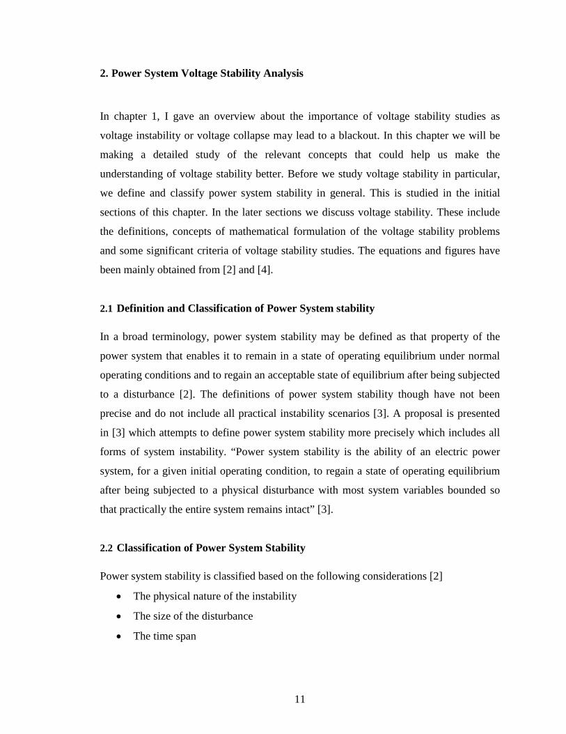
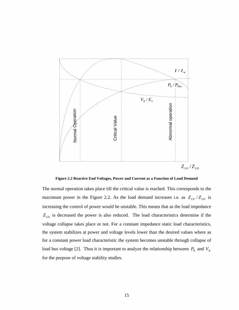
Figure 2.2[2] shows the plots of I , RV and RP as a function of LDLN ZZ / . RP increases
rapidly as the load demand i.e. LDLN ZZ / is increased. This is done by decreasing LDZ . RP
reaches a maximum value and then begins to decrease. The maximum value of RP
indicates the maximum value of active power that can be transmitted through an
impedance from a constant voltage source. This power transmitted is maximum when the
voltage drop in the line is equal in magnitude to RV that is when 1/ =LDLN ZZ [2]. With
a gradual decrease in LDZ there is an increase in I and decrease in RV . The reason for a
rapid increase in RP initially is due to the dominant increase of I in comparison to the
decrease in RV at high values of LDZ . As LDZ approaches LNZ this effect is not so
dominant and hence there is a gradual change rather than a sharp increase and decrease in
the values of I and RV respectively. As LDZ goes below LNZ , the decrease in RV
dominates the increase in I and hence there is a decrease in RP .
15
LDLN ZZ /
MaxR PP /
scII /
SR EV /
Nor
mal
Ope
ratio
n
Crit
ical
Val
ue
Abn
orm
al o
pera
tion
Figure 2.2 Reactive End Voltages, Power and Current as a Function of Load Demand The normal operation takes place till the critical value is reached. This corresponds to the
maximum power in the Figure 2.2. As the load demand increases i.e. as LDLN ZZ / is
increasing the control of power would be unstable. This means that as the load impedance
LDZ is decreased the power is also reduced. The load characteristics determine if the
voltage collapse takes place or not. For a constant impedance static load characteristics,
the system stabilizes at power and voltage levels lower than the desired values where as
for a constant power load characteristic the system becomes unstable through collapse of
load bus voltage [2]. Thus it is important to analyze the relationship between RP and RV
for the purpose of voltage stability studies.

16
2.5 P-V Curves
The relationship between RP and RV is shown in Figure2.3 [2] for a particular power
factor value. But the voltage drop in the transmission lines is a function of both the active
and the reactive power transfer as seen in Equations (2.7) and (2.9). Thus the load power
factor affects the power voltage characteristics of the system Figure 2.4[2] represents the
curves for RP and RV for different load power factor values.
SR EV /
RMAXR PP /
Critical Voltage
Figure 2.3 Power Voltage Characteristics for the System of Figure2.1
The dotted lines represent the locus of critical operating points. This means that operating
points above the critical values represent satisfactory operation. A sudden reduction in
power factor, which causes an increase in the reactive power delivered, can cause the
system to change from a stable operating condition to an unstable condition as shown in
the lower part of the curves in Figure 2.3 and Figure 2.4.

17
RMaxR PP /
SR EV /
0.9 Lag
0.9 Lead0.95 lead
0.95 Lag 1.0
Locus of Critical Points
Figure 2.4 Power Voltage characteristics for Different Load Power Factors
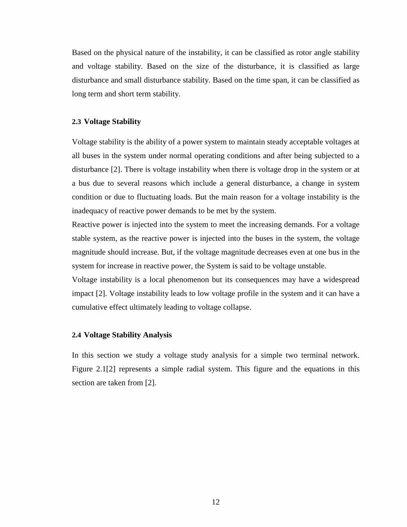
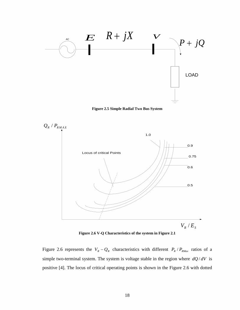
2.6 V-Q Characteristics
For purpose of analysis let us consider a simple radial system as shown in Figure 2.5[4].
The system load end voltage can be expressed in terms of QP, as given in [4]
( ) ( )2/1
222222
4221
22
+−−±
+−= QPXEQXEQXV (2.10)
For Reactive Power Flow RX >>
i.e. 090≈φ
XV
XEVQ
2
cos −=⇒ δ [4] (2.11)
0cos2 =+−⇒ QXEVV δ [4] (2.12)
XVE
dVdQ 2cos −
=δ [4] (2.13)
18
AC
LOAD
jQP +jXR +E V
Figure 2.5 Simple Radial Two Bus System
1.0
0.9
0.75
0.6
0.5
R M A XR PQ /
SR EV /
Locus of critical Points
Figure 2.6 V-Q Characteristics of the system in Figure 2.1
Figure 2.6 represents the RR QV − characteristics with different RMaxR PP / ratios of a
simple two-terminal system. The system is voltage stable in the region where dVdQ / is
positive [4]. The locus of critical operating points is shown in the Figure 2.6 with dotted
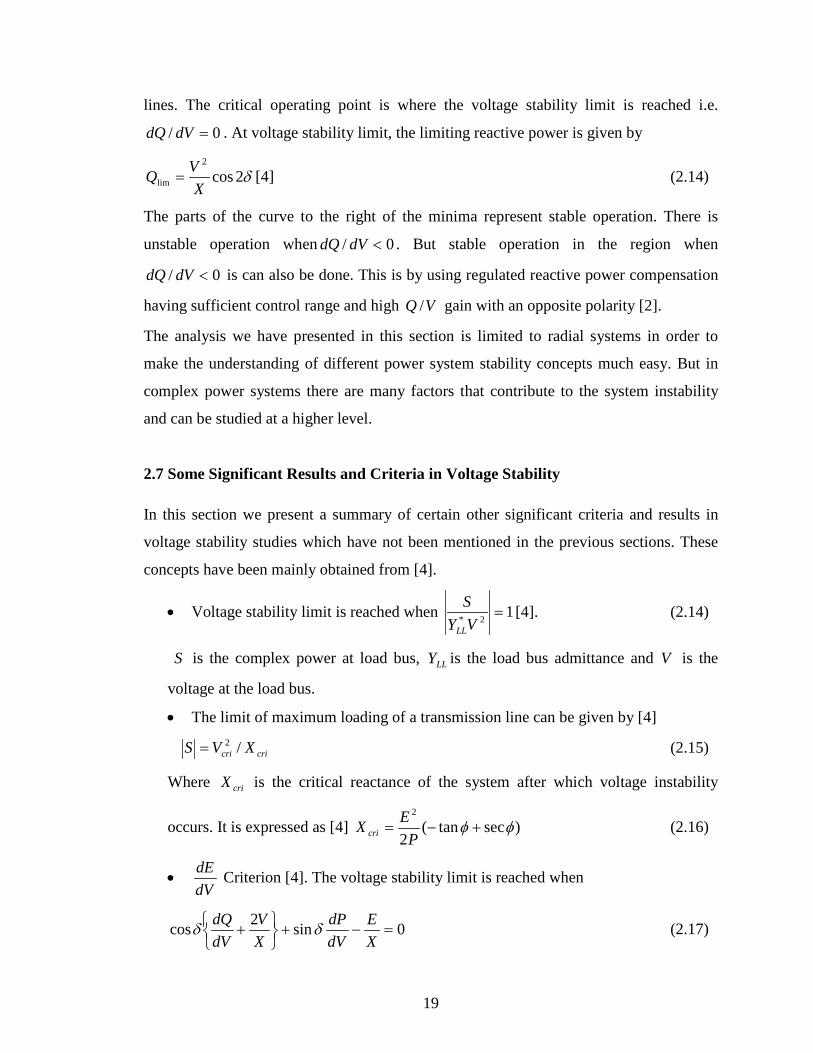
19
lines. The critical operating point is where the voltage stability limit is reached i.e.
0/ =dVdQ . At voltage stability limit, the limiting reactive power is given by
δ2cos2
lim XVQ = [4] (2.14)
The parts of the curve to the right of the minima represent stable operation. There is
unstable operation when 0/ <dVdQ . But stable operation in the region when
0/ <dVdQ is can also be done. This is by using regulated reactive power compensation
having sufficient control range and high VQ / gain with an opposite polarity [2].
The analysis we have presented in this section is limited to radial systems in order to
make the understanding of different power system stability concepts much easy. But in
complex power systems there are many factors that contribute to the system instability
and can be studied at a higher level.
2.7 Some Significant Results and Criteria in Voltage Stability
In this section we present a summary of certain other significant criteria and results in
voltage stability studies which have not been mentioned in the previous sections. These
concepts have been mainly obtained from [4].
• Voltage stability limit is reached when 12* =VYS
LL
[4]. (2.14)
S is the complex power at load bus, LLY is the load bus admittance and V is the
voltage at the load bus.
• The limit of maximum loading of a transmission line can be given by [4]
cricri XVS /2= (2.15)
Where criX is the critical reactance of the system after which voltage instability
occurs. It is expressed as [4] )sectan(2
2
φφ +−=P
EX cri (2.16)
• dVdE Criterion [4]. The voltage stability limit is reached when
0sin2cos =−+
+
XE
dVdP
XV
dVdQ δδ (2.17)

20
• dVdZ Criterion [4]. The value of critical impedance beyond which voltage
instability occurs can found from this criteria. Voltage instability occurs when
0=dVdZ
In this chapter we have tried to present a simple and clear understanding of the
voltage stability concepts. An advanced level of analytical methods for voltage
stability and rotor angle stability, which often go hand in hand, has been described in
[2].
21
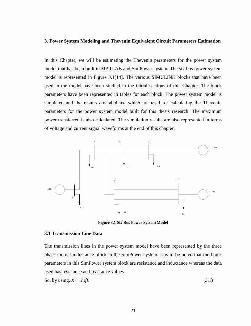
3. Power System Modeling and Thevenin Equivalent Circuit Parameters Estimation
In this Chapter, we will be estimating the Thevenin parameters for the power system
model that has been built in MATLAB and SimPower system. The six bus power system
model is represented in Figure 3.1[14]. The various SIMULINK blocks that have been
used in the model have been studied in the initial sections of this Chapter. The block
parameters have been represented in tables for each block. The power system model is
simulated and the results are tabulated which are used for calculating the Thevenin
parameters for the power system model built for this thesis research. The maximum
power transferred is also calculated. The simulation results are also represented in terms
of voltage and current signal waveforms at the end of this chapter.
G2G1
G3
L4 L5 L3
L2
L6L1
4 5 3
2
16
Figure 3.1 Six Bus Power System Model
3.1 Transmission Line Data
The transmission lines in the power system model have been represented by the three
phase mutual inductance block in the SimPower system. It is to be noted that the block
parameters in this SimPower system block are resistance and inductance whereas the data
used has resistance and reactance values.
So, by using, fLX π2= (3.1)
22
For a system frequency of 60 Hz and individual reactance values as mentioned in the
table, the corresponding inductance values have been calculated.
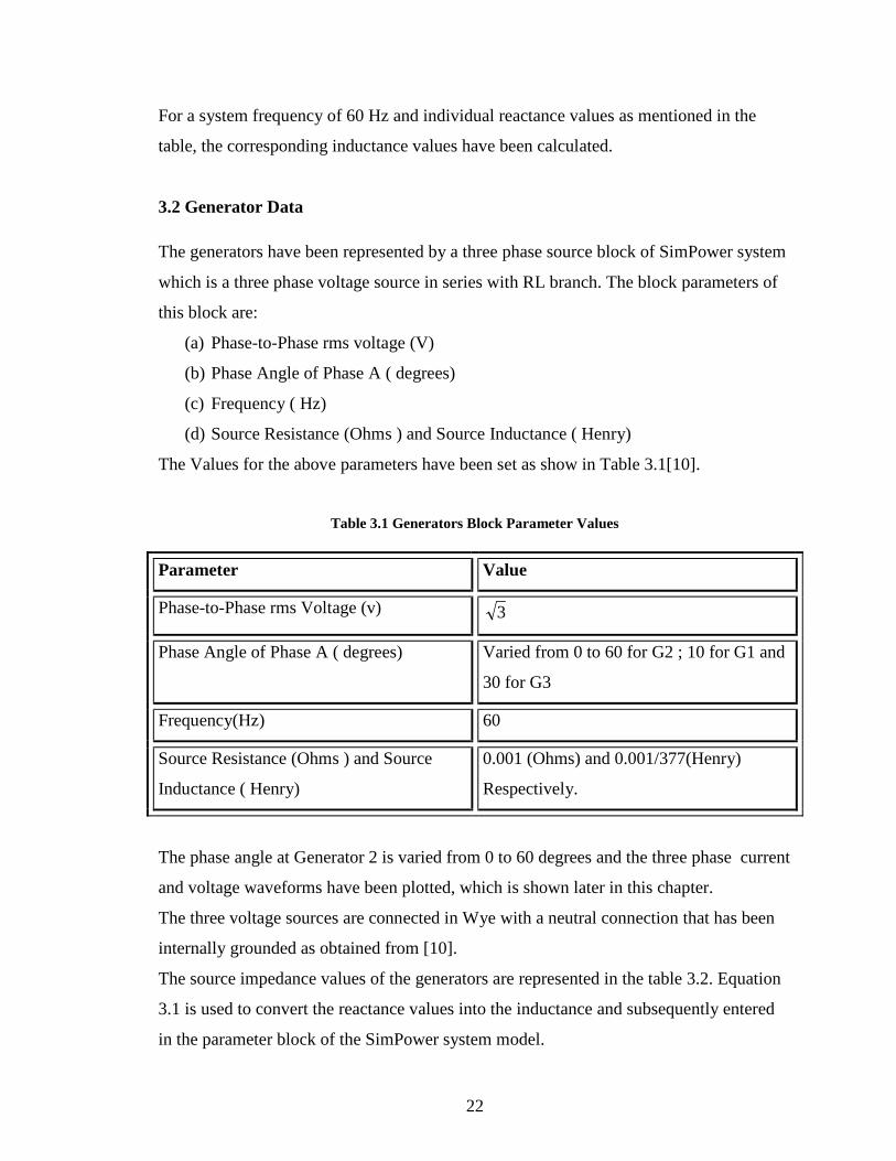
3.2 Generator Data
The generators have been represented by a three phase source block of SimPower system
which is a three phase voltage source in series with RL branch. The block parameters of
this block are:
(a) Phase-to-Phase rms voltage (V)
(b) Phase Angle of Phase A ( degrees)
(c) Frequency ( Hz)
(d) Source Resistance (Ohms ) and Source Inductance ( Henry)
The Values for the above parameters have been set as show in Table 3.1[10].
Table 3.1 Generators Block Parameter Values
Parameter Value
Phase-to-Phase rms Voltage (v) 3
Phase Angle of Phase A ( degrees) Varied from 0 to 60 for G2 ; 10 for G1 and
30 for G3
Frequency(Hz) 60
Source Resistance (Ohms ) and Source
Inductance ( Henry)
0.001 (Ohms) and 0.001/377(Henry)
Respectively.
The phase angle at Generator 2 is varied from 0 to 60 degrees and the three phase current
and voltage waveforms have been plotted, which is shown later in this chapter.
The three voltage sources are connected in Wye with a neutral connection that has been
internally grounded as obtained from [10].
The source impedance values of the generators are represented in the table 3.2. Equation
3.1 is used to convert the reactance values into the inductance and subsequently entered
in the parameter block of the SimPower system model.
23
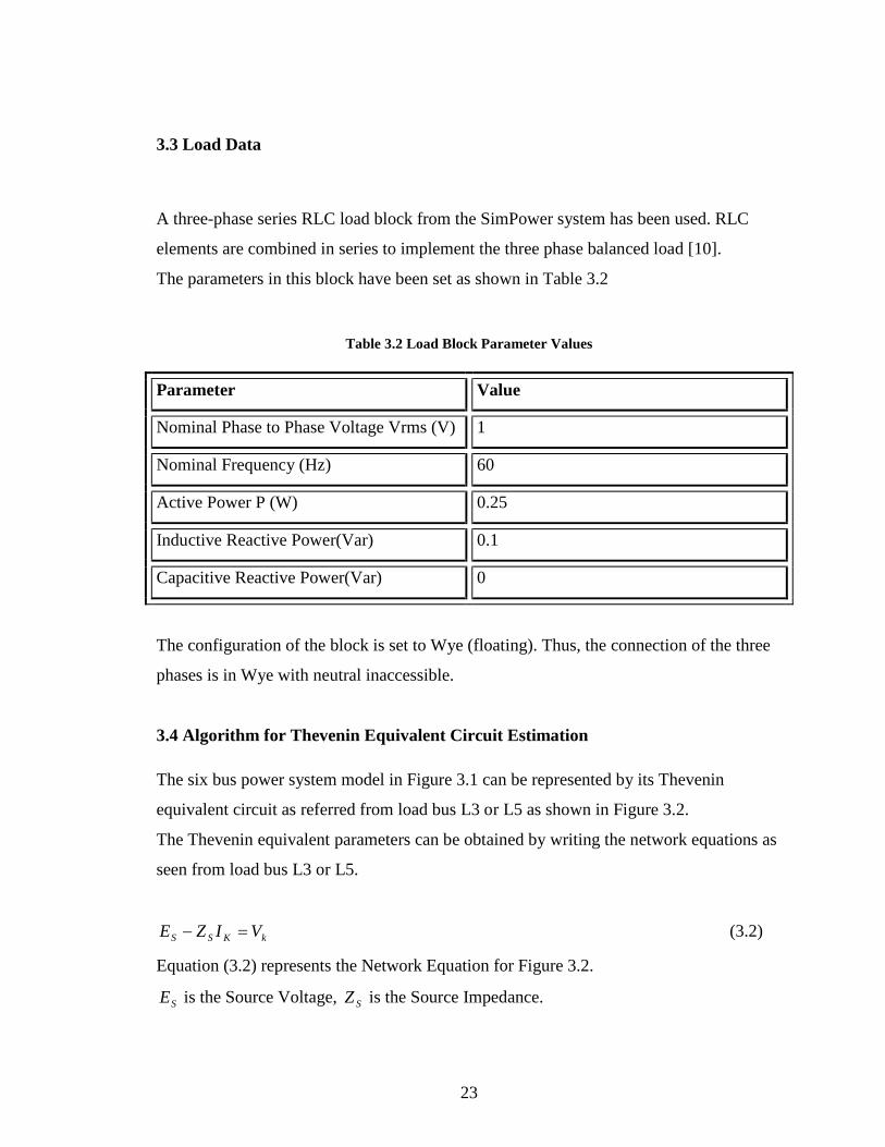
3.3 Load Data
A three-phase series RLC load block from the SimPower system has been used. RLC
elements are combined in series to implement the three phase balanced load [10].
The parameters in this block have been set as shown in Table 3.2
Table 3.2 Load Block Parameter Values
Parameter Value
Nominal Phase to Phase Voltage Vrms (V) 1
Nominal Frequency (Hz) 60
Active Power P (W) 0.25
Inductive Reactive Power(Var) 0.1
Capacitive Reactive Power(Var) 0
The configuration of the block is set to Wye (floating). Thus, the connection of the three
phases is in Wye with neutral inaccessible.
3.4 Algorithm for Thevenin Equivalent Circuit Estimation
The six bus power system model in Figure 3.1 can be represented by its Thevenin
equivalent circuit as referred from load bus L3 or L5 as shown in Figure 3.2.
The Thevenin equivalent parameters can be obtained by writing the network equations as
seen from load bus L3 or L5.
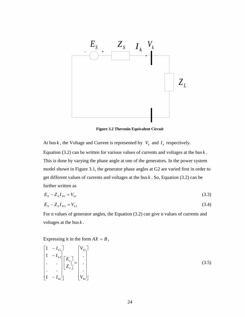
kKSS VIZE =− (3.2)
Equation (3.2) represents the Network Equation for Figure 3.2.
SE is the Source Voltage, SZ is the Source Impedance.
24
SE SZ kVkI
LZ
- +
Figure 3.2 Thevenin Equivalent Circuit
At bus k , the Voltage and Current is represented by kV and kI respectively.
Equation (3.2) can be written for various values of currents and voltages at the bus k .
This is done by varying the phase angle at one of the generators. In the power system
model shown in Figure 3.1, the generator phase angles at G2 are varied first in order to
get different values of currents and voltages at the bus k . So, Equation (3.2) can be
further written as
11 kKSS VIZE =− (3.3)
22 kKSS VIZE =− (3.4)
For n values of generator angles, the Equation (3.2) can give n values of currents and
voltages at the bus k .
Expressing it in the form BAX = ,
=
−
−−
kn
k
s
s
kn
k
k
V
V
ZE
I
II
.
.
.
1....
11 1
2
1
(3.5)

25
A is an )2(nx Matrix.
X is a )12( x Matrix and B is an 1nx Matrix.
The solution for Equation (3.5) is obtained using the Least Mean Squares technique.
)()( 1 BAAAX TT −=
Thus the Thevenin equivalent parameters are calculated.
In the power system model represented in Figure 3.1, the phase angles at G2 are varied
from 0 to 60 degrees to get the Thevenin equivalent voltage and current at the load, L3.
The results are tabulated as shown in Table 3.3
Table 3.3 Voltage and Currents at Bus L3
Angle at
Generator
2 (
Degrees)
Voltage at bus 3
(p.u.)
Magnitude(angle
in degree)
Current at
bus 3 (p.u.)
Active
Power P (
p.u.)
Reactive
Power Q (
p.u. )
0 1.252 (12.62) 0.97(12) 1.821 0.01968
10 1.257(13.11) 0.8362(13.5) 1.577 -0.00953
20 1.26(13.63) 0.7006(13.5) 1.324 0.001912
30 1.262(14.17) 0.567 (11.3) 1.072 0.05371
40 1.261 (14.72) 0.444 (4.8) 0.8271 0.1442
60 1.254 (15.75) 0.3082 (-32) 0.3894 0.4294
At load bus L5, the currents and voltages are tabulated by varying the phase angle of the
generator G1. This is represented in Table 3.4

26
Table 3.4Voltage and Current at Load Bus L5
Angle at
Generator
1 (
Degrees)
Voltage at bus 5
(p.u.)
Magnitude(angle
in degree)
Current at bus
5 (p.u.)
Active
Power P (
p.u.)
Reactive
Power Q (
p.u. )
0 1.223(-5.411) 0.9163(2.452) 1.665 -0.2299
10 1.229(-1.684) 0.5881(3.134) 1.08 -0.09098
20 1.226(2.047) 0.267(-6.839) 0.4851 0.07585
30 1.1214(5.761) 0.1562(-
105.2)
-0.1016 0.2655
40 1.194(9.441) 0.4544(-
135.1)
-0.6624 0.4723
60 1.128(16.61) 1.109(-134.3) -1.638 0.9116
Using these values of voltage and current at the buses, the Thevenin parameters have
been calculated. The Thevenin parameters for different sets of measurements are
tabulated in Tables 3.5 and 3.6
Table 3.5Thevenin Parameters for 4, 5 and 6 sets of measurements at Load bus L3 Number of Sets of
Measurements SE SZ
SRE SME SR SX
4 1.2273 0.3586 0.0240 0.0846
5 1.227 0.3588 0.0237 0.0849
6 1.2270 0.3587 0.0236 0.0848
27
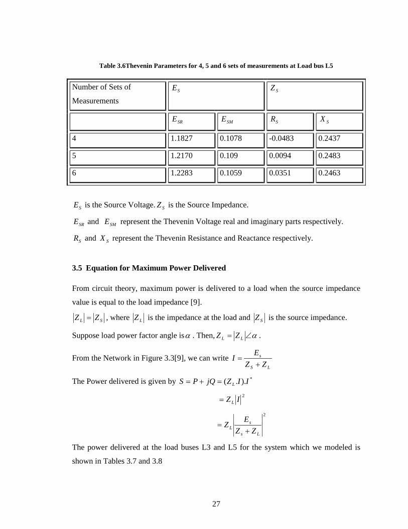
Table 3.6Thevenin Parameters for 4, 5 and 6 sets of measurements at Load bus L5
Number of Sets of
Measurements SE SZ
SRE SME SR SX
4 1.1827 0.1078 -0.0483 0.2437
5 1.2170 0.109 0.0094 0.2483
6 1.2283 0.1059 0.0351 0.2463
SE is the Source Voltage. SZ is the Source Impedance.
SRE and SME represent the Thevenin Voltage real and imaginary parts respectively.
SR and SX represent the Thevenin Resistance and Reactance respectively.
3.5 Equation for Maximum Power Delivered
From circuit theory, maximum power is delivered to a load when the source impedance
value is equal to the load impedance [9].
SL ZZ = , where LZ is the impedance at the load and SZ is the source impedance.
Suppose load power factor angle isα . Then, α∠= LL ZZ .
From the Network in Figure 3.3[9], we can write LS
s
ZZE
I+
=
The Power delivered is given by *)..( IIZjQPS L=+=
2IZ L=
2
Ls
sL ZZ
EZ
+=
The power delivered at the load buses L3 and L5 for the system which we modeled is
shown in Tables 3.7 and 3.8

28
SE SZ
kV
kI
SL ZZ =
- +P Q
Figure 3.3 Equivalent Power System Model for Calculating Maximum Power Delivered
Table 3.7 Power Delivered at the Bus L3 for Different Power Factor angles Angle P (p.u) Q (p.u)
0 7.3202 -
10 6.3869 1.1262
20 5.5158 2.0076
30 4.6906 2.7081
40 3.8972 3.2702
Table 3.8 Power Delivered at the Bus L5 for Different Power Factor angles
Angle P (p.u) Q (p.u)
0 2.6770
10 2.2949 0.4047
20 1.9511 0.7102
30 1.6358 0.9444
40 1.3414 1.1256
29
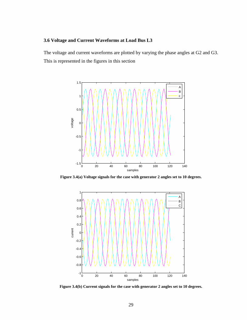
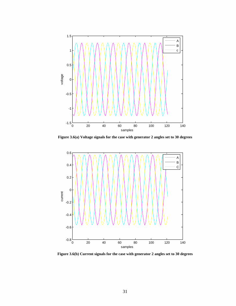
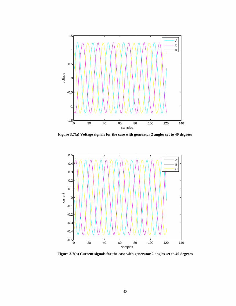
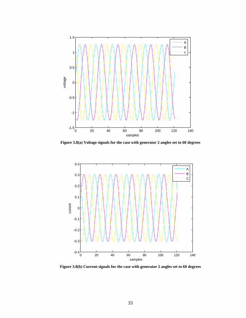
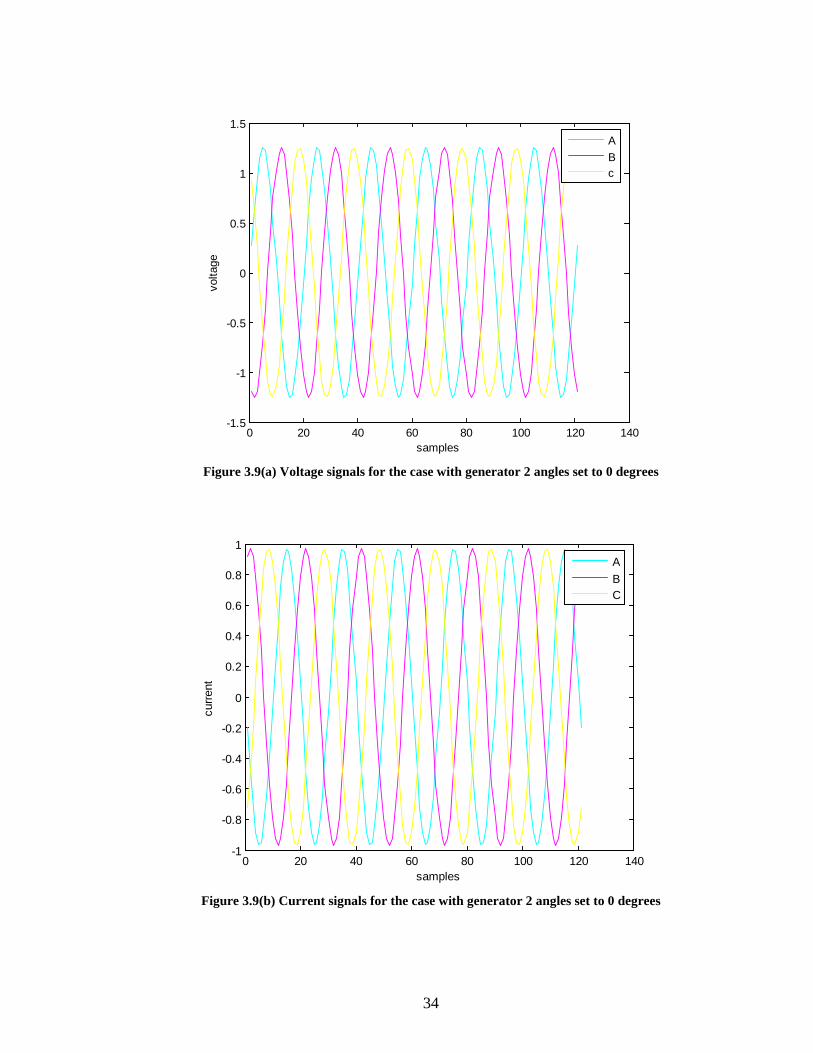
3.6 Voltage and Current Waveforms at Load Bus L3
The voltage and current waveforms are plotted by varying the phase angles at G2 and G3.
This is represented in the figures in this section
0 20 40 60 80 100 120 140-1.5
-1
-0.5
0
0.5
1
1.5
samples
volta
ge
ABc
Figure 3.4(a) Voltage signals for the case with generator 2 angles set to 10 degrees.
0 20 40 60 80 100 120 140-1
-0.8
-0.6
-0.4
-0.2
0
0.2
0.4
0.6
0.8
1
samples
curre
nt
ABC
Figure 3.4(b) Current signals for the case with generator 2 angles set to 10 degrees.
30
.
0 20 40 60 80 100 120 140-1.5
-1
-0.5
0
0.5
1
1.5
samples
volta
geABc
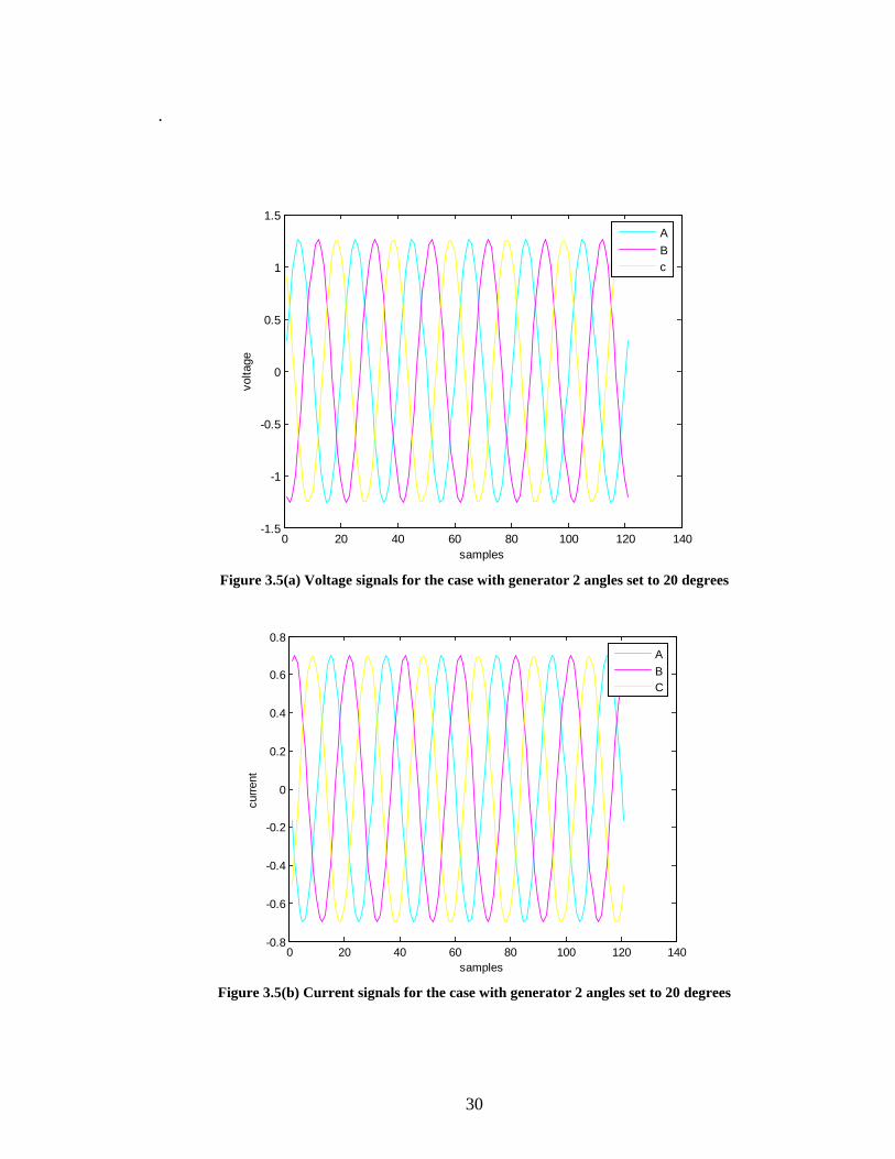
Figure 3.5(a) Voltage signals for the case with generator 2 angles set to 20 degrees
0 20 40 60 80 100 120 140-0.8
-0.6
-0.4
-0.2
0
0.2
0.4
0.6
0.8
samples
curre
nt
ABC
Figure 3.5(b) Current signals for the case with generator 2 angles set to 20 degrees
31
0 20 40 60 80 100 120 140-1.5
-1
-0.5
0
0.5
1
1.5
samples
volta
ge
ABc
Figure 3.6(a) Voltage signals for the case with generator 2 angles set to 30 degrees
0 20 40 60 80 100 120 140-0.8
-0.6
-0.4
-0.2
0
0.2
0.4
0.6
samples
curre
nt
ABC
Figure 3.6(b) Current signals for the case with generator 2 angles set to 30 degrees
32
0 20 40 60 80 100 120 140-1.5
-1
-0.5
0
0.5
1
1.5
samples
volta
ge
ABc
Figure 3.7(a) Voltage signals for the case with generator 2 angles set to 40 degrees
0 20 40 60 80 100 120 140-0.5
-0.4
-0.3
-0.2
-0.1
0
0.1
0.2
0.3
0.4
0.5
samples
curre
nt
ABC
Figure 3.7(b) Current signals for the case with generator 2 angles set to 40 degrees
33
0 20 40 60 80 100 120 140-1.5
-1
-0.5
0
0.5
1
1.5
samples
volta
ge
ABc
Figure 3.8(a) Voltage signals for the case with generator 2 angles set to 60 degrees
0 20 40 60 80 100 120 140-0.4
-0.3
-0.2
-0.1
0
0.1
0.2
0.3
0.4
samples
curre
nt
ABC
Figure 3.8(b) Current signals for the case with generator 2 angles set to 60 degrees
34
0 20 40 60 80 100 120 140-1.5
-1
-0.5
0
0.5
1
1.5
samples
volta
ge
ABc
Figure 3.9(a) Voltage signals for the case with generator 2 angles set to 0 degrees
0 20 40 60 80 100 120 140-1
-0.8
-0.6
-0.4
-0.2
0
0.2
0.4
0.6
0.8
1
samples
curre
nt
ABC
Figure 3.9(b) Current signals for the case with generator 2 angles set to 0 degrees
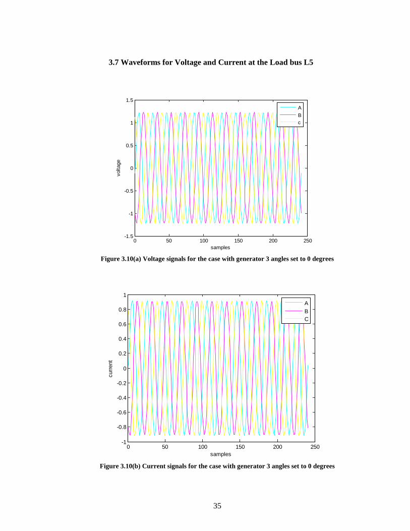
35
3.7 Waveforms for Voltage and Current at the Load bus L5
0 50 100 150 200 250-1.5
-1
-0.5
0
0.5
1
1.5
samples
volta
ge
ABc
Figure 3.10(a) Voltage signals for the case with generator 3 angles set to 0 degrees
0 50 100 150 200 250-1
-0.8
-0.6
-0.4
-0.2
0
0.2
0.4
0.6
0.8
1
samples
curre
nt
ABC
Figure 3.10(b) Current signals for the case with generator 3 angles set to 0 degrees
36
0 50 100 150 200 250-1.5
-1
-0.5
0
0.5
1
1.5
samples
volta
ge
ABc
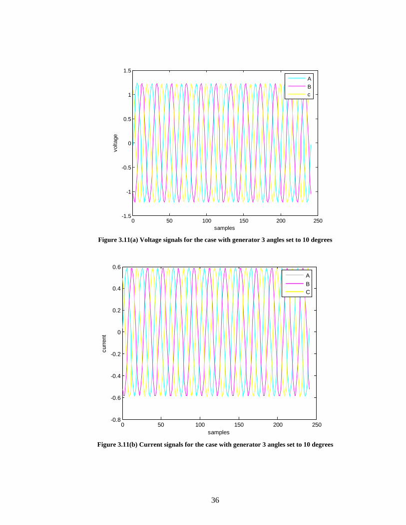
Figure 3.11(a) Voltage signals for the case with generator 3 angles set to 10 degrees
0 50 100 150 200 250-0.8
-0.6
-0.4
-0.2
0
0.2
0.4
0.6
samples
curre
nt
ABC
Figure 3.11(b) Current signals for the case with generator 3 angles set to 10 degrees
37
0 50 100 150 200 250-1.5
-1
-0.5
0
0.5
1
1.5
samples
volta
ge
ABc
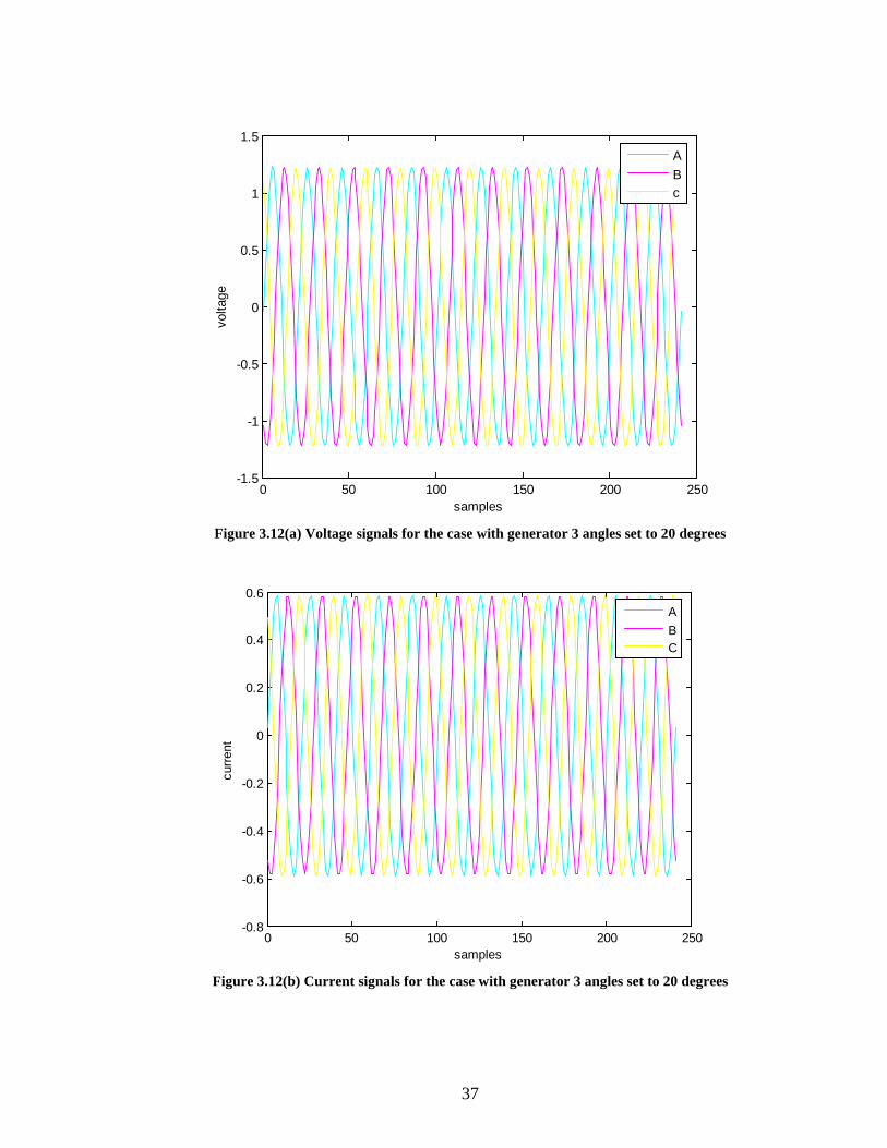
Figure 3.12(a) Voltage signals for the case with generator 3 angles set to 20 degrees
0 50 100 150 200 250-0.8
-0.6
-0.4
-0.2
0
0.2
0.4
0.6
samples
curre
nt
ABC
Figure 3.12(b) Current signals for the case with generator 3 angles set to 20 degrees
38
0 50 100 150 200 250-1.5
-1
-0.5
0
0.5
1
1.5
samples
volta
ge
ABc
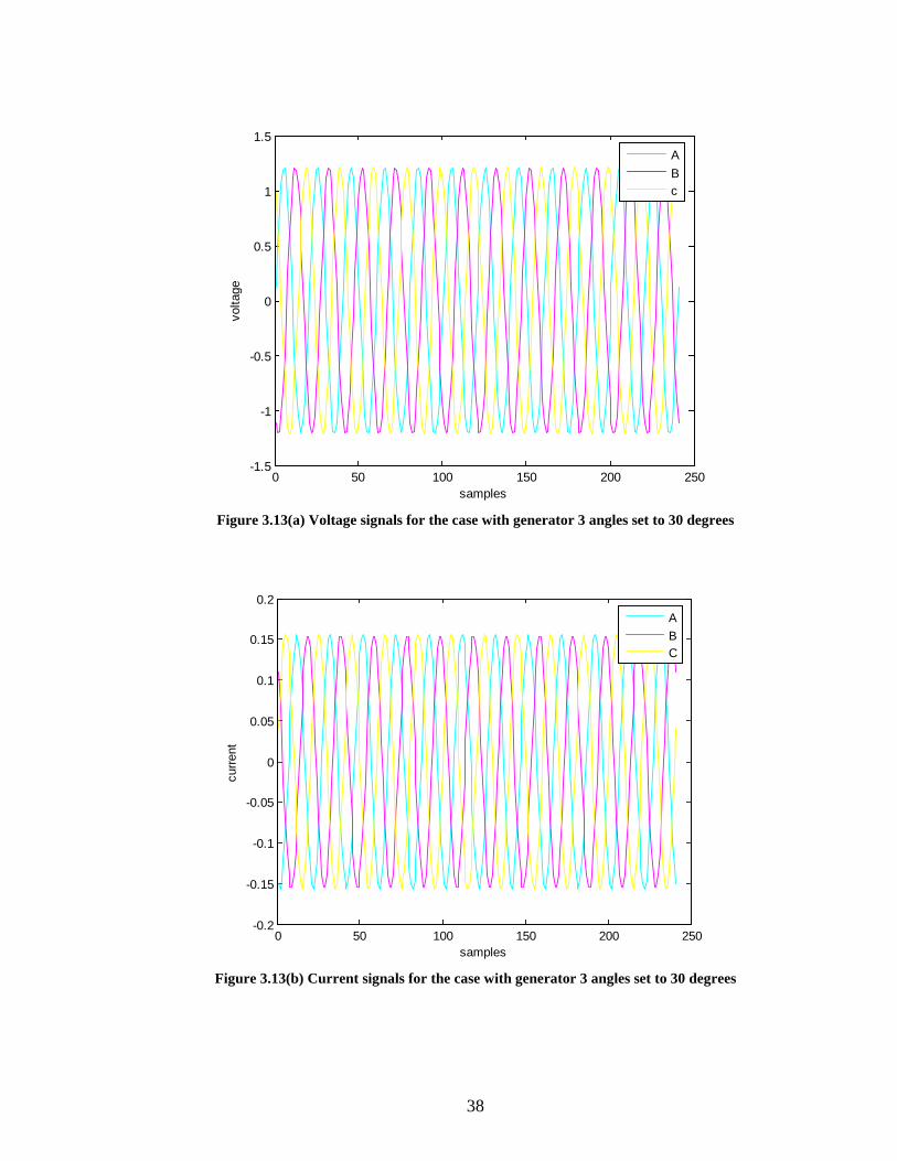
Figure 3.13(a) Voltage signals for the case with generator 3 angles set to 30 degrees
0 50 100 150 200 250-0.2
-0.15
-0.1
-0.05
0
0.05
0.1
0.15
0.2
samples
curre
nt
ABC
Figure 3.13(b) Current signals for the case with generator 3 angles set to 30 degrees
39
0 50 100 150 200 250-1.5
-1
-0.5
0
0.5
1
1.5
samples
volta
ge
ABc
Figure 3.14(a) Voltage signals for the case with generator 3 angles set to 40 degrees
0 50 100 150 200 250-0.5
-0.4
-0.3
-0.2
-0.1
0
0.1
0.2
0.3
0.4
0.5
samples
curre
nt
ABC
Figure 3.14(b) Current signals for the case with generator 3 angles set to 40 degrees

40
0 50 100 150 200 250-1.5
-1
-0.5
0
0.5
1
1.5
samples
volta
ge
ABc
Figure 3.15(a) Voltage signals for the case with generator 3 angles set to 60 degrees
0 50 100 150 200 250-1.5
-1
-0.5
0
0.5
1
1.5
samples
curre
nt
ABC
Figure 3.15(b) Current signals for the case with generator 3 angles set to 60 degrees
41
4. Fault Analysis and Estimation of Fault Location
In this Chapter, we will be studying the concepts of unsymmetrical fault analysis and also
the algorithms that have been proposed in Dr. Liao’s work, “Fault location utilizing
unsynchronized voltage measurements during fault”, Electric Power Components &
Systems, vol. 34, no. 12, December 2006, pp. 1283 – 1293. One of the algorithms has
been used to estimate the fault location for my power system model. The shunt
capacitances have been neglected in the algorithm used for estimation in order to have
simplicity and computational efficiency. The Thevenin parameter values obtained for the
power system model of Chapter 3 have been used in the fault location algorithm in [5] to
calculate the fault location for the model used in this thesis. The current and voltage
signal waveforms for the different values of fault location have been presented at the end
of this chapter.
In the initial sections of this chapter, the basic concepts of unsymmetrical fault analysis
have been presented. The equations and figures of unsymmetrical fault analysis in
sections (4.1-4.5) have all been obtained from [4] and we explain it as much as possible.
4.1 Unsymmetrical Faults
The unsymmetrical faults can be classified as shunt type faults and series type faults.
Shunt type faults can again be classified as [4]:
(a) Single Line to Ground fault
(b) Line to Line Fault
(c) Double Line to Ground fault
Before we study in detail about the shunt type faults, it is important to study the
symmetrical component analysis of unsymmetrical faults.
4.2 Symmetrical Component Analysis of Unsymmetrical Faults
In this section, we will analyze how a power network which is under a fault condition can
be represented in terms of positive, negative and zero sequence networks as seen from the
point where the fault is occurring.

42
Figure 4.1 represents a general power network [4]. F is the point of fault occurrence.
When the fault occurs in the system, the currents are represented by aI , bI , cI as shown,
which flow out of the system. The voltages of lines ,a ,b c with respect to the ground are
,aV ,bV cV respectively.
aVbV
cV
aI bI cI
aF
bc
Figure 4.1 A General Power Network
Before the fault occurs, the positive sequence voltages of all synchronous machines in the
network are given by aE . This is the pre fault voltage at F.
The positive, negative and zero sequence networks after the occurrence of the fault as
seen from F are represented in Figures 4.2 (a), (b) and (c) [4].
1aV
1aI
F
1aI
Figure 4.2 (a) Positive sequence network as seen from the fault point

43
2aV
2aI
2aI
F
Figure 4.2 (b) Negative Sequence Network as seen from the fault point
0aVF
0aI
0aI
Figure 4.2(c) Zero sequence Network as seen from the fault point The Thevenin equivalents of the sequence networks are represented in Figure 4.2 (d), (e),
(f) [4]
1aI
1aV1Z
F
+aE
Figure 4.2 (d) Thevenin Equivalent of Positive sequence Network as seen from F
44
2aV
2aI
2Z
F
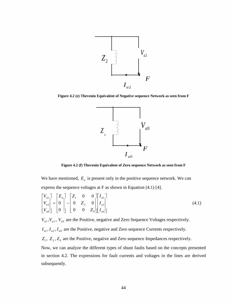
Figure 4.2 (e) Thevenin Equivalent of Negative sequence Network as seen from F
0aI
0aV0
Z
F
Figure 4.2 (f) Thevenin Equivalent of Zero sequence Network as seen from F
We have mentioned, aE is present only in the positive sequence network. We can
express the sequence voltages at F as shown in Equation (4.1) [4].
−
=
0
2
1
0
2
1
0
2
1
000000
00
a
a
aa
a
a
a
III
ZZ
ZE
VVV
(4.1)
1aV , 2aV , 0aV are the Positive, negative and Zero Sequence Voltages respectively.
1aI , 2aI , 0aI are the Positive, negative and Zero sequence Currents respectively.
1Z , 2Z , 0Z are the Positive, negative and Zero sequence Impedances respectively.
Now, we can analyze the different types of shunt faults based on the concepts presented
in section 4.2. The expressions for fault currents and voltages in the lines are derived
subsequently.
45
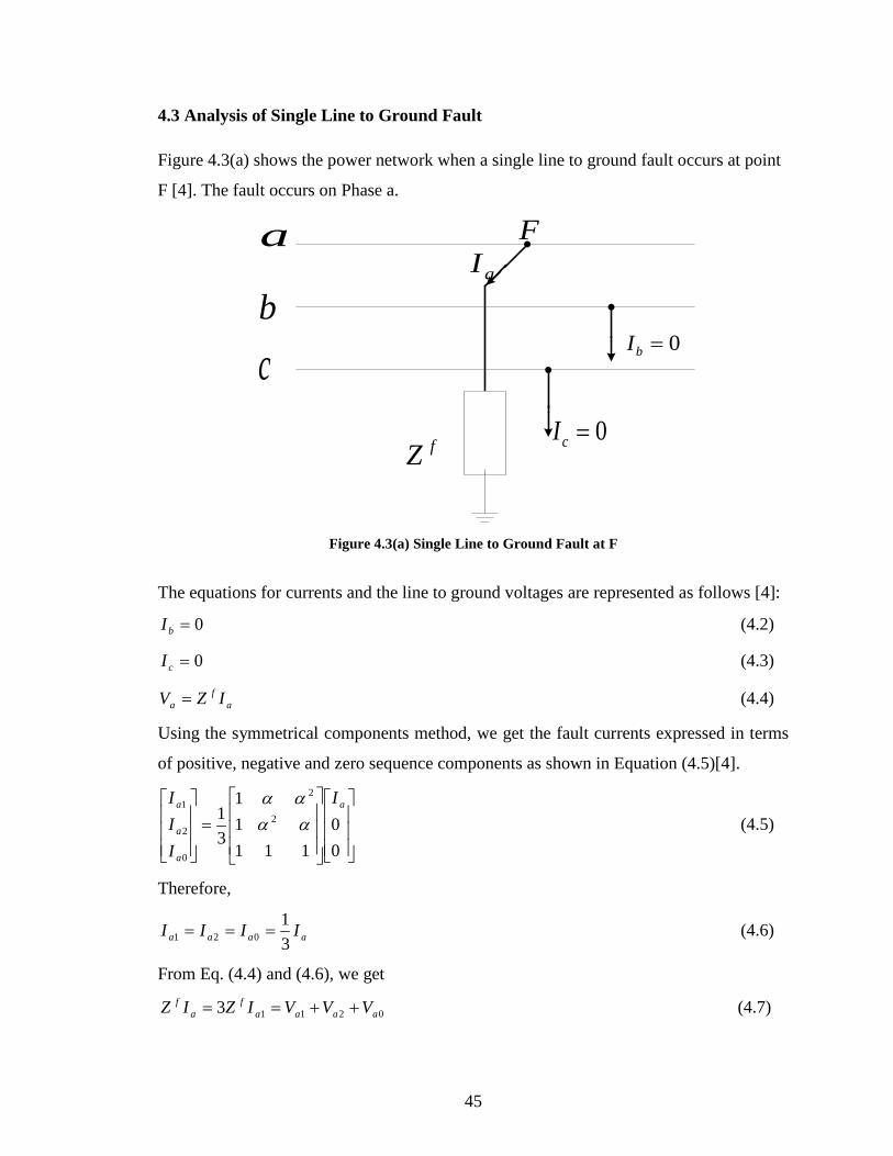
4.3 Analysis of Single Line to Ground Fault
Figure 4.3(a) shows the power network when a single line to ground fault occurs at point
F [4]. The fault occurs on Phase a.
FaI
0=bI
0=cIfZ
a
b
c
Figure 4.3(a) Single Line to Ground Fault at F
The equations for currents and the line to ground voltages are represented as follows [4]:
0=bI (4.2)
0=cI (4.3)
af
a IZV = (4.4)
Using the symmetrical components method, we get the fault currents expressed in terms
of positive, negative and zero sequence components as shown in Equation (4.5)[4].
=
00
11111
31 2
2
0
2
1 a
a
a
a I
III
αααα
(4.5)
Therefore,
aaaa IIII31
021 === (4.6)
From Eq. (4.4) and (4.6), we get
02113 aaaaf
af VVVIZIZ ++== (4.7)
46
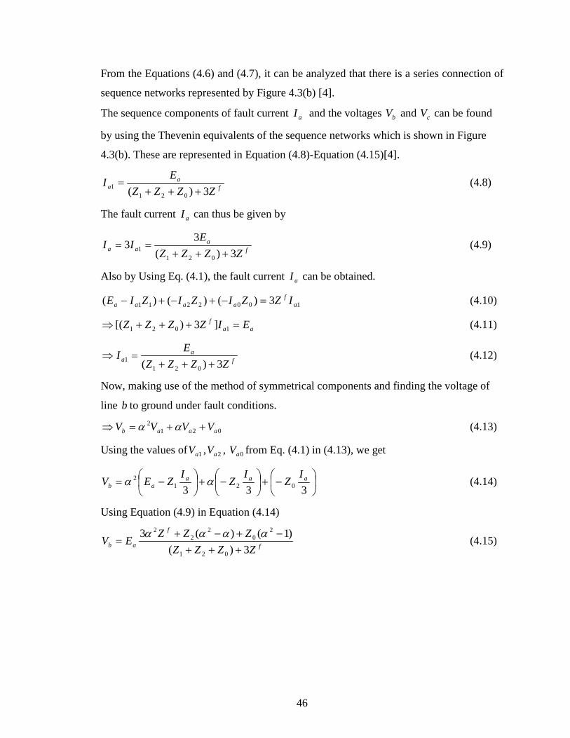
From the Equations (4.6) and (4.7), it can be analyzed that there is a series connection of
sequence networks represented by Figure 4.3(b) [4].
The sequence components of fault current aI and the voltages bV and cV can be found
by using the Thevenin equivalents of the sequence networks which is shown in Figure
4.3(b). These are represented in Equation (4.8)-Equation (4.15)[4].
fa
a ZZZZE
I3)( 021
1 +++= (4.8)
The fault current aI can thus be given by
fa
aa ZZZZE
II3)(
33
0211 +++== (4.9)
Also by Using Eq. (4.1), the fault current aI can be obtained.
1002211 3)()()( af
aaaa IZZIZIZIE =−+−+− (4.10)
aaf EIZZZZ =+++⇒ 1021 ]3)[( (4.11)
fa
a ZZZZE
I3)( 021
1 +++=⇒ (4.12)
Now, making use of the method of symmetrical components and finding the voltage of
line b to ground under fault conditions.
0212
aaab VVVV ++=⇒ αα (4.13)
Using the values of 1aV , 2aV , 0aV from Eq. (4.1) in (4.13), we get
−+
−+
−=
333 0212 aaa
abI
ZI
ZI
ZEV αα (4.14)
Using Equation (4.9) in Equation (4.14)
f
f
ab ZZZZZZZ
EV3)(
)1()(3
021
20
22
2
+++−+−+
=αααα
(4.15)
47
1aV
1aI
2aV
0aV
F
F
F
12 aa II =
10 aa II =
aaaa IIII31
021 ===
fa ZI fZ3
0aV
2aV
0Z
2ZF
F
1aI
1aV1Z
F
+aE
12 aa II =
10 aa II =
fZ3fa ZI
aaaa IIII31
021 ===
Figure 4.3(b) Connection of sequence networks for single Line to Ground Fault
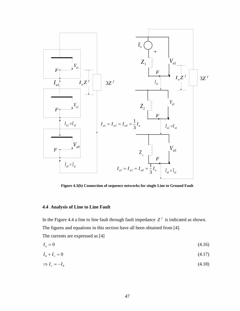
4.4 Analysis of Line to Line Fault
In the Figure 4.4 a line to line fault through fault impedance fZ is indicated as shown.
The figures and equations in this section have all been obtained from [4].
The currents are expressed as [4]
0=aI (4.16)
0=+ cb II (4.17)
bc II −=⇒ (4.18)

48
F0=aI
cIfZ
a
b
cbI
Figure 4.4(a) Line to Line Fault through Impedance fZ
The voltage relationship between bV and cV is expressed as [4]
fbcb ZIVV =− (4.19)
The positive, negative and zero sequence components of the fault currents are expressed
as [4]
−
=
b
b
a
a
a
II
III 0
11111
31 2
2
0
2
1
αααα
(4.20)
On solving Equation (4.20), we get
12 aa II −= (4.21)
00 =aI (4.22)
Now, the symmetrical components of voltages under fault at F are expressed as [4]
−
=
bf
b
b
a
a
a
a
IZVVV
VVV
11111
31 2
2
0
2
1
αααα
(4.23)
From the Equation (4.23) expressing 1aV and 2aV
bf
baa IZVVV 221 )(3 ααα −++= (4.24)
bf
baa IZVVV ααα −++= )(3 22 (4.25)
49
Solving Equation (4.24) and (4.25)
bf
bf
aa IZjIZVV 3)()(3 221 =−=− αα (4.26)
Using Equations (4.21) and (4.22) in (4.20)
112 3)( aab IjII −=−= αα (4.27)
Substituting Equation (4.27) in Equation (4.26)
121 af
aa IZVV =− (4.28)
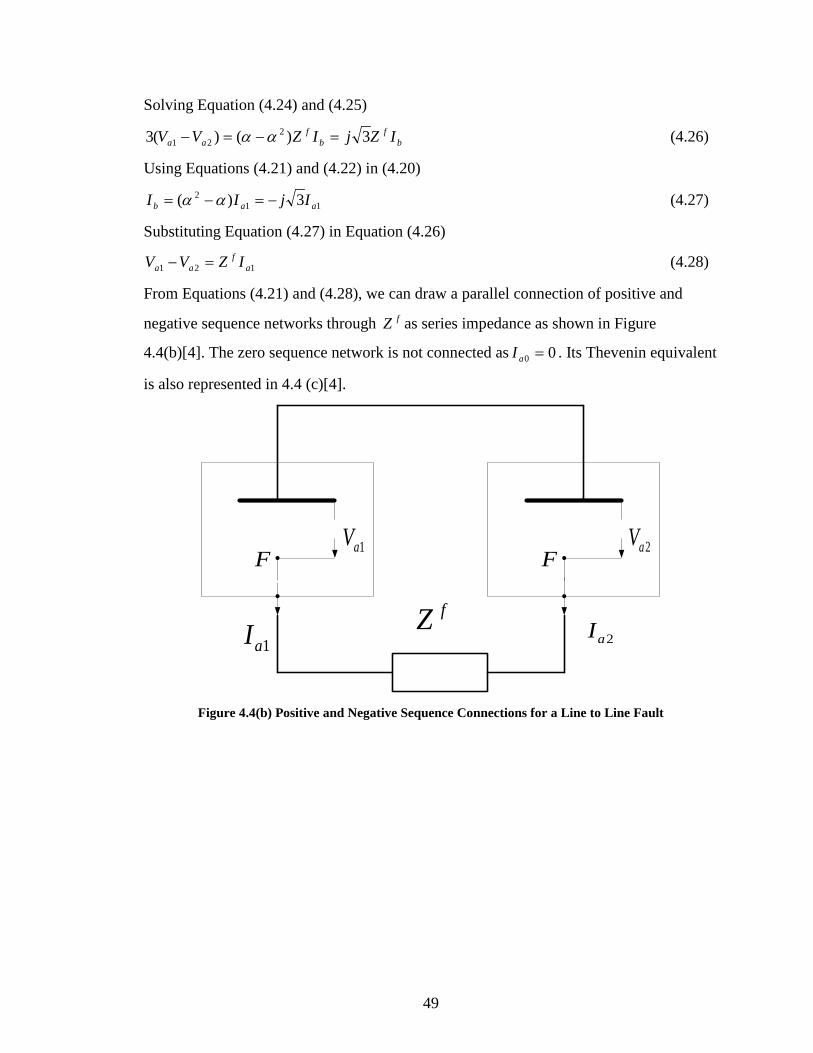
From Equations (4.21) and (4.28), we can draw a parallel connection of positive and
negative sequence networks through fZ as series impedance as shown in Figure
4.4(b)[4]. The zero sequence network is not connected as 00 =aI . Its Thevenin equivalent
is also represented in 4.4 (c)[4].
1aV 2aVF
1aI 2aI
F
fZ
Figure 4.4(b) Positive and Negative Sequence Connections for a Line to Line Fault

50
2aV
2aI
2ZF
1aI
1ZF
+aE
1aV
fZ
Figure 4.4(c) Thevenin Equivalent for connection of Sequence Networks for L-L Fault
By using the Thevenin equivalent, we can write the expressions for
fa
a ZZZE
I++
=21
1 (4.29)
fa
cb ZZZEj
II++
−=−=
21
3 (4.30)
The voltages at fault can be found out by knowing 1aV and 2aV . This can be calculated
from 1aI .
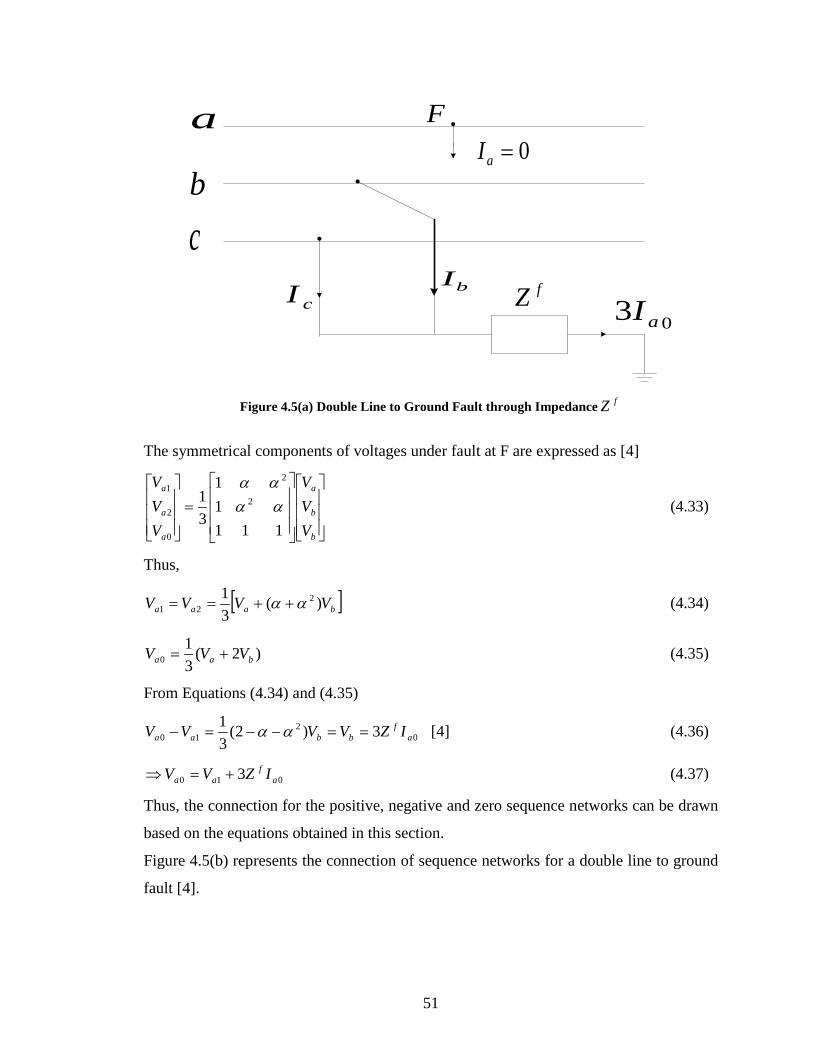
4.5 Double Line to Ground Fault Analysis
In this section, we will make the analysis of a double line to ground fault. The figures and
equations have all been obtained from [4].Figure 4.5(a) shows the double line to ground
fault in a power system at a point F [4].
The fault current for a double line to ground fault is expressed as [4]
00 021 =++⇒= aaaa IIII (4.31)
The voltage to ground at fault conditions are expressed as [4]
03)( af
cbf
cb IZIIZVV =+== (4.32)
51
F0=aI
cI fZ
a
b
cbI
03 aI
Figure 4.5(a) Double Line to Ground Fault through Impedance fZ
The symmetrical components of voltages under fault at F are expressed as [4]
=
b
b
a
a
a
a
VVV
VVV
11111
31 2
2
0
2
1
αααα
(4.33)
Thus,
[ ]baaa VVVV )(31 2
21 αα ++== (4.34)
)2(31
0 baa VVV += (4.35)
From Equations (4.34) and (4.35)
02
10 3)2(31
af
bbaa IZVVVV ==−−=− αα [4] (4.36)
010 3 af
aa IZVV +=⇒ (4.37)
Thus, the connection for the positive, negative and zero sequence networks can be drawn
based on the equations obtained in this section.
Figure 4.5(b) represents the connection of sequence networks for a double line to ground
fault [4].

52
1aV 2aVF
1aI 2aI
F
fZ3
0aVF
0aI
Figure 4.5(b) connection of sequence networks for a double line to ground fault
2aV
2aI
2ZF
1aI
1ZF
+aE
1aV0aV
0Z
FfZ3 0aI
Figure 4.5(c) Thevenin Equivalent for the sequence network connections for a LLG fault
From Figure 4.5 (c) the following expressions can be written [4]
)3/()3( 020211 f
f
aa ZZZZZZZ
EI
++++=⇒ (4.38)
4.6 Fault Location Algorithm
In this section we study a fault location algorithm that has been presented in [5]. The
impedance based algorithm is studied and made use in order to calculate the fault
location. This algorithm is applicable for all kind of unsymmetrical faults [5]. For
studying the algorithm we consider the transmission line represented in Figure 4.6.
53
GE HE
P QG abcZ
abcZ HabcZ
Figure 4.6 Transmission Line Considered for the Algorithm [5]
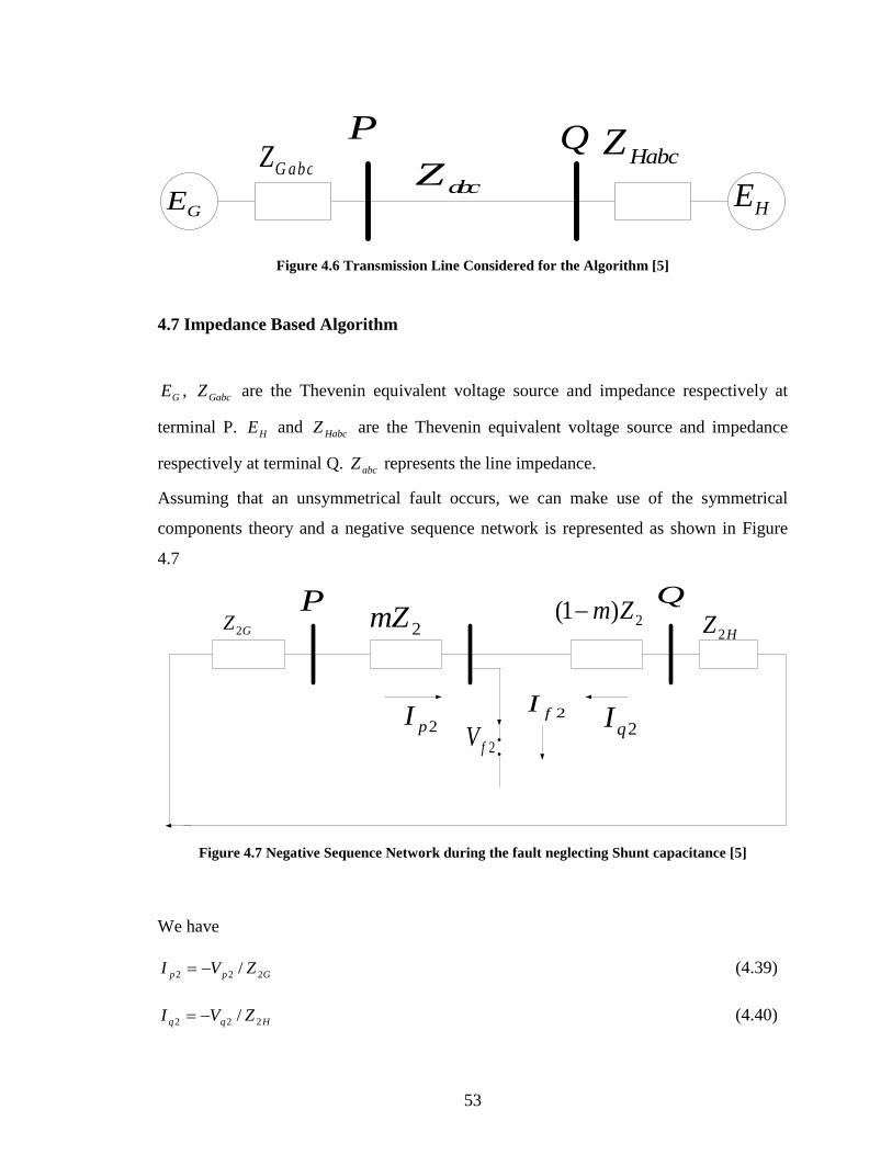
4.7 Impedance Based Algorithm
GE , GabcZ are the Thevenin equivalent voltage source and impedance respectively at
terminal P. HE and HabcZ are the Thevenin equivalent voltage source and impedance
respectively at terminal Q. abcZ represents the line impedance.
Assuming that an unsymmetrical fault occurs, we can make use of the symmetrical
components theory and a negative sequence network is represented as shown in Figure
4.7
GZ2 HZ22)1( Zm−
2mZP Q
2pI 2qI2fI
2fV
Figure 4.7 Negative Sequence Network during the fault neglecting Shunt capacitance [5]
We have
Gpp ZVI 222 /−= (4.39)
Hqq ZVI 222 /−= (4.40)
54
δjqqpp eIZmVImZV ])1([ 222222 −−=− (4.41)
Where,
2pV , 2pI Negative sequence voltage and current during the fault at terminal P;
2qV , 2qI Negative sequence voltage and current during the fault at terminal Q;
GZ 2 , HZ 2 Negative sequence source impedance at terminal P and Q;
δ Synchronization angle between measurements at terminal P and Q;
m Per unit fault distance from terminal P;
2Z Total negative sequence impedance of the line.
In the above equations, 2pV and 2qV are known based on the measurements. Then 2pI
and 2qI can be obtained using Equations (4.39) and (4.40).
Solving Equation (4.41) will result in the fault location. The Detailed method is referred
to the original work presented in [5]. The algorithm neglecting shunt capacitances, as
presented above, has advantages of simplicity and computational efficiency. However,
neglecting shunt capacitances may lead to certain errors for long lines. Consideration of
shunt capacitances is discussed in [5].
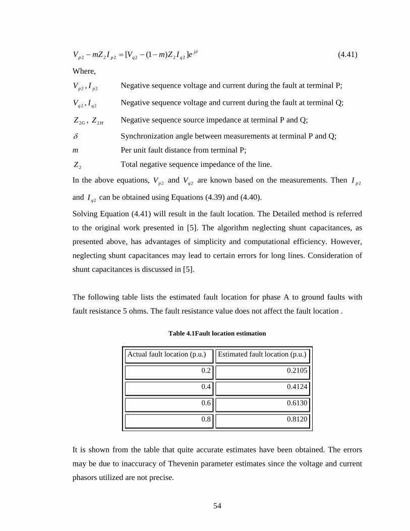
The following table lists the estimated fault location for phase A to ground faults with
fault resistance 5 ohms. The fault resistance value does not affect the fault location .
Table 4.1Fault location estimation
Actual fault location (p.u.) Estimated fault location (p.u.)
0.2 0.2105
0.4 0.4124
0.6 0.6130
0.8 0.8120
It is shown from the table that quite accurate estimates have been obtained. The errors
may be due to inaccuracy of Thevenin parameter estimates since the voltage and current
phasors utilized are not precise.

55
4.8 Voltage and Current Waveforms for Different Fault Locations
The voltage and current waveforms for different fault locations are plotted which is
represented in the figures in this section.
0 20 40 60 80 100 120 140-1.5
-1
-0.5
0
0.5
1
1.5
samples
volta
ge
ABc
Figure 4.8(a) Voltage waveforms for a phase A to ground fault with a fault location of 0.2 p.u
0 20 40 60 80 100 120 140-4
-3
-2
-1
0
1
2
3
samples
curre
nt
ABC
Figure 4.8(b) Current waveforms for a phase A to ground fault with a fault location of 0.2 p.u
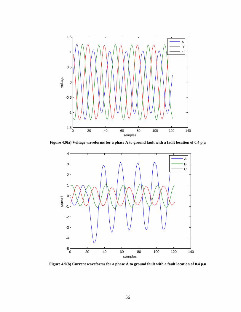
56
0 20 40 60 80 100 120 140-1.5
-1
-0.5
0
0.5
1
1.5
samples
volta
ge
ABc
Figure 4.9(a) Voltage waveforms for a phase A to ground fault with a fault location of 0.4 p.u
0 20 40 60 80 100 120 140-5
-4
-3
-2
-1
0
1
2
3
4
samples
curre
nt
ABC
Figure 4.9(b) Current waveforms for a phase A to ground fault with a fault location of 0.4 p.u
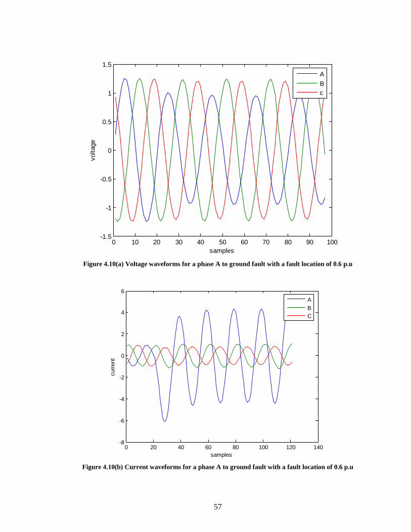
57
0 10 20 30 40 50 60 70 80 90 100-1.5
-1
-0.5
0
0.5
1
1.5
samples
volta
ge
ABc
Figure 4.10(a) Voltage waveforms for a phase A to ground fault with a fault location of 0.6 p.u
0 20 40 60 80 100 120 140-8
-6
-4
-2
0
2
4
6
samples
curre
nt
ABC
Figure 4.10(b) Current waveforms for a phase A to ground fault with a fault location of 0.6 p.u
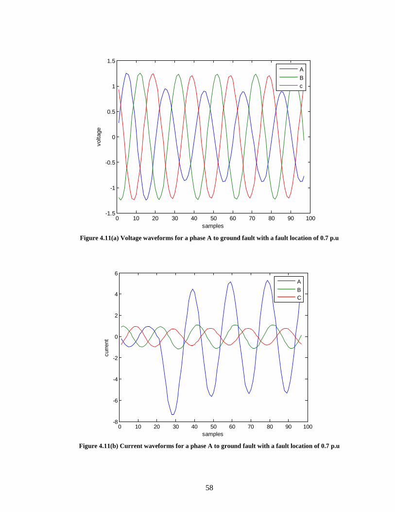
58
0 10 20 30 40 50 60 70 80 90 100-1.5
-1
-0.5
0
0.5
1
1.5
samples
volta
ge
ABc
Figure 4.11(a) Voltage waveforms for a phase A to ground fault with a fault location of 0.7 p.u
0 10 20 30 40 50 60 70 80 90 100-8
-6
-4
-2
0
2
4
6
samples
curre
nt
ABC
Figure 4.11(b) Current waveforms for a phase A to ground fault with a fault location of 0.7 p.u

59
5. Conclusion
The main objectives of this thesis were Thevenin parameters estimation, determining the
maximum power that can be transferred and the estimation of fault location. In Chapter 3,
we made use of MATLAB SIMULINK® to simulate the power system model that has
been used in this Thesis. The results yielded the values of Thevenin equivalent
parameters. These in turn were used to calculate the maximum power that can be
transferred to the load bus under different conditions. In Chapter 4 we used the values of
the Thevenin parameters for fault location. The results obtained confirm the available
results of the algorithms that have been used.
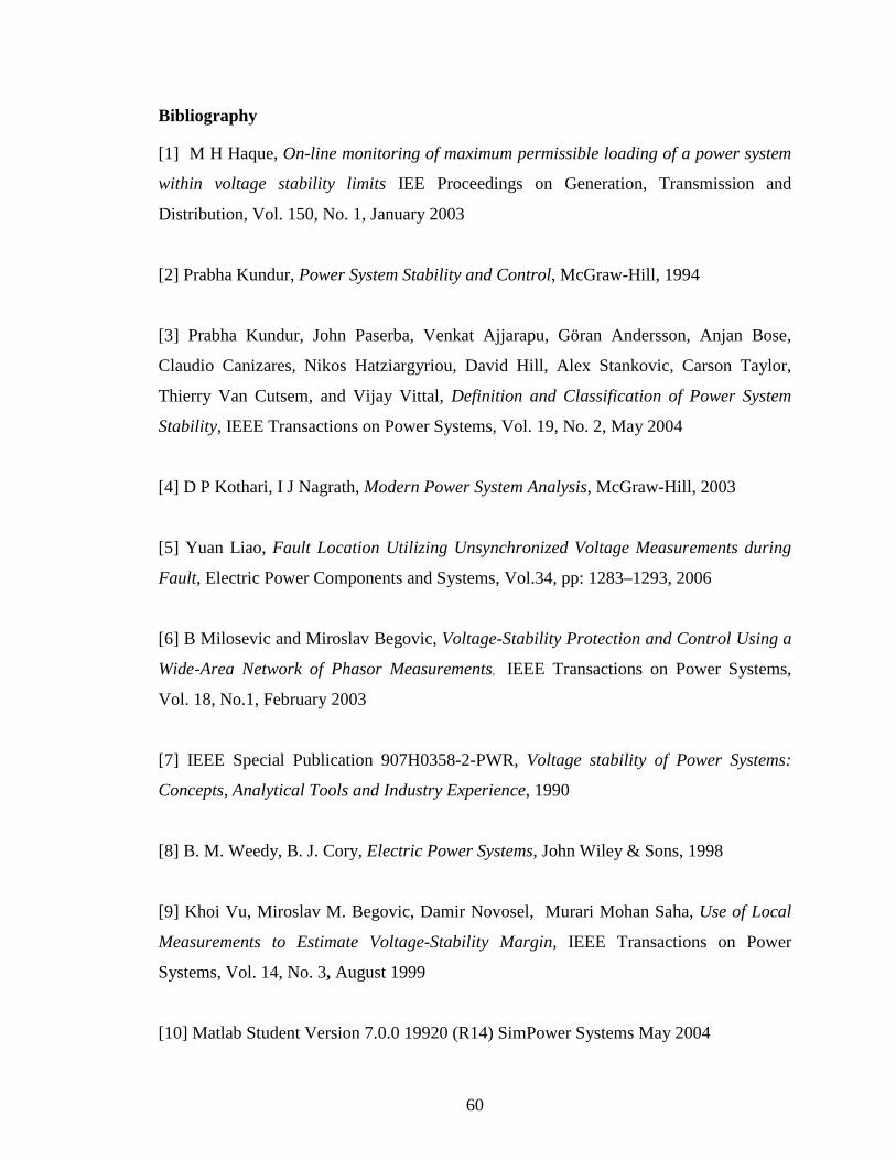
60
Bibliography
[1] M H Haque, On-line monitoring of maximum permissible loading of a power system
within voltage stability limits IEE Proceedings on Generation, Transmission and
Distribution, Vol. 150, No. 1, January 2003
[2] Prabha Kundur, Power System Stability and Control, McGraw-Hill, 1994
[3] Prabha Kundur, John Paserba, Venkat Ajjarapu, Göran Andersson, Anjan Bose,
Claudio Canizares, Nikos Hatziargyriou, David Hill, Alex Stankovic, Carson Taylor,
Thierry Van Cutsem, and Vijay Vittal, Definition and Classification of Power System
Stability, IEEE Transactions on Power Systems, Vol. 19, No. 2, May 2004
[4] D P Kothari, I J Nagrath, Modern Power System Analysis, McGraw-Hill, 2003
[5] Yuan Liao, Fault Location Utilizing Unsynchronized Voltage Measurements during
Fault, Electric Power Components and Systems, Vol.34, pp: 1283–1293, 2006
[6] B Milosevic and Miroslav Begovic, Voltage-Stability Protection and Control Using a
Wide-Area Network of Phasor Measurements, IEEE Transactions on Power Systems,
Vol. 18, No.1, February 2003
[7] IEEE Special Publication 907H0358-2-PWR, Voltage stability of Power Systems:
Concepts, Analytical Tools and Industry Experience, 1990
[8] B. M. Weedy, B. J. Cory, Electric Power Systems, John Wiley & Sons, 1998
[9] Khoi Vu, Miroslav M. Begovic, Damir Novosel, Murari Mohan Saha, Use of Local
Measurements to Estimate Voltage-Stability Margin, IEEE Transactions on Power
Systems, Vol. 14, No. 3, August 1999
[10] Matlab Student Version 7.0.0 19920 (R14) SimPower Systems May 2004
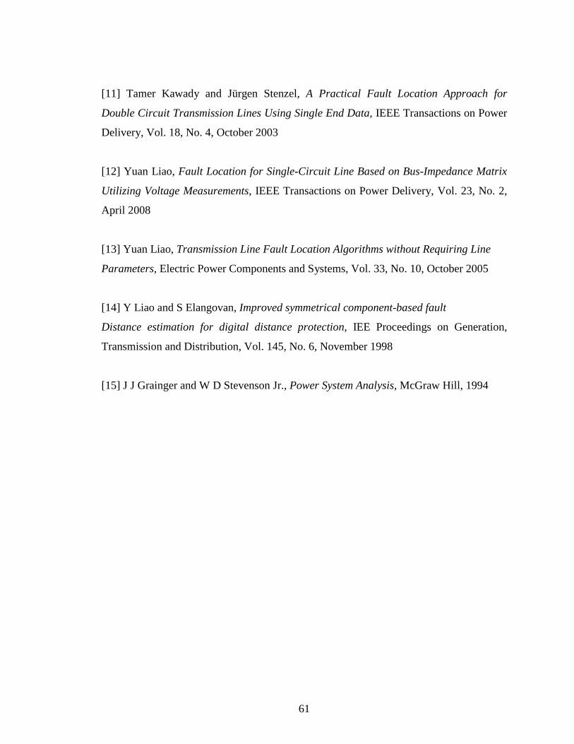
61
[11] Tamer Kawady and Jürgen Stenzel, A Practical Fault Location Approach for
Double Circuit Transmission Lines Using Single End Data, IEEE Transactions on Power
Delivery, Vol. 18, No. 4, October 2003
[12] Yuan Liao, Fault Location for Single-Circuit Line Based on Bus-Impedance Matrix
Utilizing Voltage Measurements, IEEE Transactions on Power Delivery, Vol. 23, No. 2,
April 2008
[13] Yuan Liao, Transmission Line Fault Location Algorithms without Requiring Line
Parameters, Electric Power Components and Systems, Vol. 33, No. 10, October 2005
[14] Y Liao and S Elangovan, Improved symmetrical component-based fault
Distance estimation for digital distance protection, IEE Proceedings on Generation,
Transmission and Distribution, Vol. 145, No. 6, November 1998
[15] J J Grainger and W D Stevenson Jr., Power System Analysis, McGraw Hill, 1994

62
Vita
Mohammad Museb Iftakhar was born in Karimnagar, Andhra Pradesh, India on
December 14th, 1985. He received his Bachelor of Engineering degree in Electrical and
Electronics Engineering in 2006 from Osmania University, Hyderabad, India. He worked
as a Research Assistant in spring 2007 in the Power Systems Research Group at the
University of Kentucky, Lexington, Kentucky, U.S.A.
Mohammad M Iftakhar