This document was downloaded from the Penspen Integrity ... · 4839 90th Avenue S.E Calgary, Alberta Canada Phil Hopkins Penspen Ltd. Hawthorn Suite St. Peter’s Wharf Newcastle

This document was downloaded from the Penspen Integrity Virtual Library

For further information, contact Penspen Integrity:

Penspen Integrity Units 7-8

St. Peter's Wharf Newcastle upon Tyne

NE6 1TZ United Kingdom

Telephone: +44 (0)191 238 2200

Fax: +44 (0)191 275 9786 Email: [email protected]

Website: www.penspenintegrity.com

Page 1 of 21

SMART PIGS AND DEFECT ASSESSMENT CODES: COMPLETING THE CIRCLE

Stephen Westwood BJ Pipeline Inspection Services

4839 90th Avenue S.E Calgary, Alberta

Canada

Phil Hopkins Penspen Ltd. Hawthorn Suite

St. Peter’s Wharf Newcastle upon Tyne NE6 1TZ, UK

ABSTRACT

Smart pigs are used extensively as part of integrity management plans for oil and gas pipelines to detect metal loss defects, with magnetic flux leakage (MFL) technology being the most-widely used. The MFL signal gives an inferred defect size, not a direct measurement: when the signal is translated into a defect size, it has associated sizing tolerances and confidence levels. The complexity of signal analysis means that these sizing tolerances and confidence levels are difficult to determine and apply in practice. They have a major effect when assessing the significance of the defect, and when calculating corrosion growth rates from the results of multiple inspections over time. This paper describes how sizing algorithms are constructed and how the quoted tolerances are derived. Probability theory can be used to estimate the likelihood that a defect is smaller or deeper than the reported value. Finally, the effect of defect sizing tolerances and their confidence levels on corrosion growth projections is illustrated, and how they must be taken into account in any defect assessment is emphasised.

CORROSION 2004

March 28 to April 2004 New Orleans, USA

NACE International, USA

Page 2 of 21

THE INCREASING USE AND IMPORTANCE OF SMART PIGS

Smart pigs were first marketed and run in the USA nearly 40 years ago. They are now a common fixture in the pipeline business, with many on the market, using differing technologies and detecting differing types of defects, Table 1.

DEFECT METAL LOSS TOOLS6 CRACK DETECTION TOOLS

GEOMETRY TOOLS

MFL SR MFL HR UT UT MFL7 CALIPER MAPPING CORROSION D&S1 D&S D&S D&S D&S NO NO CRACKS - AXIAL

NO NO NO D&S D&S NO NO

CRACKS – CIRC.

NO d3&s4 NO D&S2 NO NO NO

DENTS d d&s d&s d&s d&s D&S D&s LAMINATIONS d d D&S D&S NO NO NO MILL DEFECTS d d D D d NO NO OVALITY NO NO NO NO NO D&S D&S5 D = DETECTS. S = SIZES 1 – No internal/external diameter discrimination 2 – Modification needed (sensors need rotating 90 deg) 3 – Lower case ‘d’ means unreliable or reduced capability in detection 4 – Lower case ‘s’ means unreliable or reduced capability in sizing 5 – If tool is equipped with ovality measuring gear 6 – ‘SR’ is standard resolution, ‘HR’ is high resolution, ‘UT’ is a tool using ultrasonic technology. ‘MFL’ is magnetic flux leakage technology. 7 – MFL field is in transverse direction Table 1. Defect Types and Pigs (‘Tools’) to Detect Them (Based On API 11601). These pigs are now used by most pipeline operators. New pipeline integrity management regulations in the USA2 and guidance documents1,3 are expected to double their use in USA pipelines over the next 5 years. Consequently, pigs are now an integral part of most pipeline operator’s integrity management programs, and their use and importance will increase.

USING SMART PIG DATA

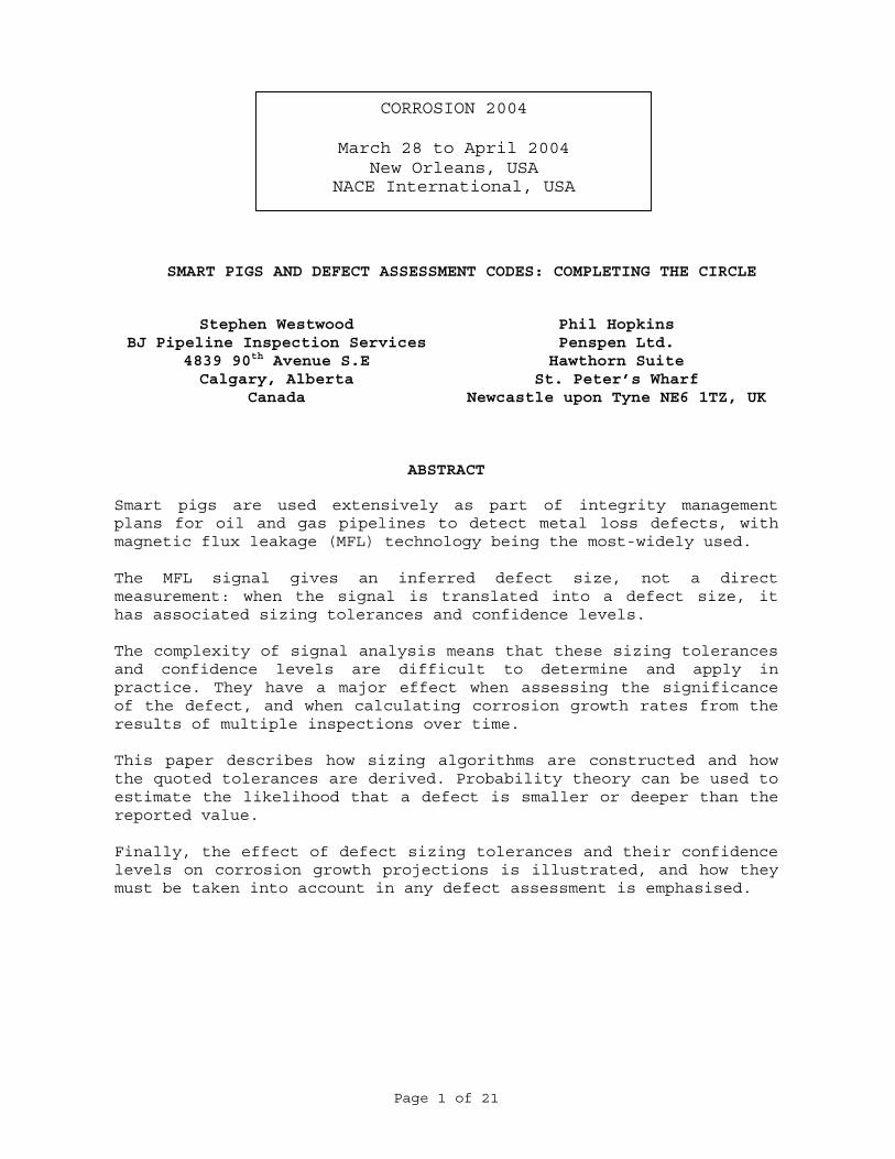
A pig detects and measures defects in a pipeline. The pipeline owner receives a list of these defects, and – for metal loss defects – a simple listing of defect location, depth, length and width. All these measurements will have a tolerance attached to them, and a confidence factor: for example a pig company may quote defect depth as ‘+/15% wall thickness (wt), 80% of the time’. This is the pig company’s estimate of how accurate their pig will measure depth, and how often they will be within these limits, Figure 1(1).

1 Figures 1-6 are not to scale

Page 3 of 21

Actual Defect Depth (%wt)

Reported Defect Depth (%wt)

20

20

40

40

60

60

+/15%wt, 80% of time

1:1

metal loss defect

0.0

0.1

0.2

0.3

0.4

0.5

0.6

0.7

0.8

0.9

1.0

0 1 2 3 4 5 6 7 8

Acceptable

Not Acceptable

Defect Length

Defect Depth

Figure 2. Defect Acceptance Curve

Figure 1. Defect Sizing Errors

Page 4 of 21

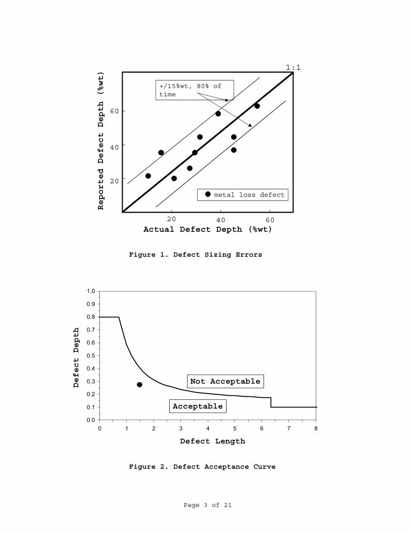
The pipeline operator will then want to conduct two calculations:

i. Is the reported defect ‘acceptable’? • The operator can use a variety of ‘fitness for purpose’

methods (e.g. Refs 4-11), but the most popular are the ASME B31G methods 5-7.

• Figure 2 shows how defects can be assessed using these methods. This figure shows the ASME B31G defect acceptance criterion6. A corrosion defect has been detected and measured by a smart pig: its length and depth are plotted on the ASME B31G curve. The defect is ‘acceptable’ to ASME B31G and need not be repaired. ‘Acceptable’ corrosion is5,6:

capable of withstanding a hydrostatic pressure test that will produce a stress of 100% of the pipe SMYS.

capable of withstanding a hydrostatic pressure test at a ratio above MAOP equal to the ratio of 100% SMYS test that will produce a stress of a 100% of the pipe SMYS test to 72% SMYS operation (1.39:1)at the calculated reduced MAOP.

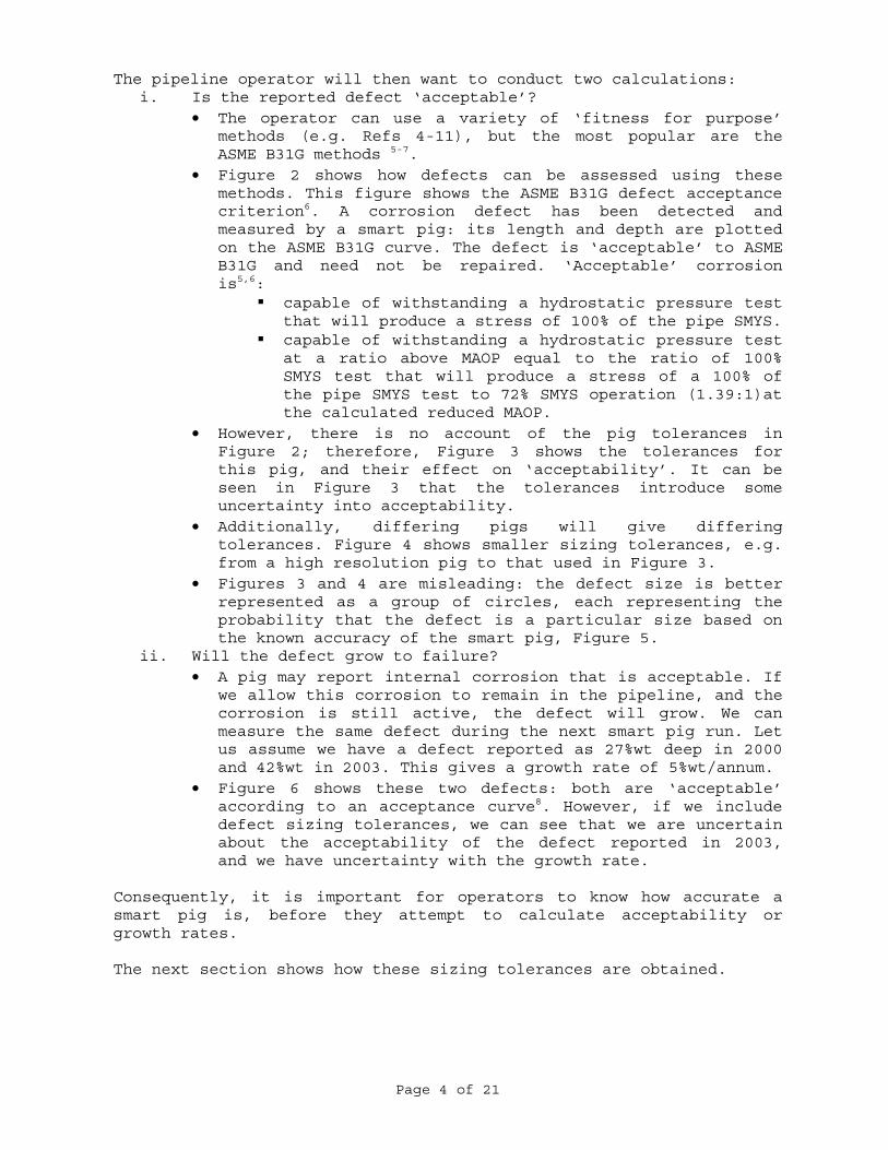
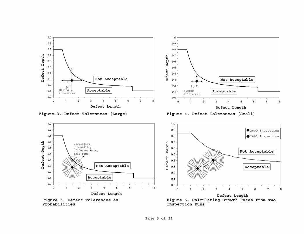
• However, there is no account of the pig tolerances in Figure 2; therefore, Figure 3 shows the tolerances for this pig, and their effect on ‘acceptability’. It can be seen in Figure 3 that the tolerances introduce some uncertainty into acceptability.

• Additionally, differing pigs will give differing tolerances. Figure 4 shows smaller sizing tolerances, e.g. from a high resolution pig to that used in Figure 3.

• Figures 3 and 4 are misleading: the defect size is better represented as a group of circles, each representing the probability that the defect is a particular size based on the known accuracy of the smart pig, Figure 5.

ii. Will the defect grow to failure? • A pig may report internal corrosion that is acceptable. If

we allow this corrosion to remain in the pipeline, and the corrosion is still active, the defect will grow. We can measure the same defect during the next smart pig run. Let us assume we have a defect reported as 27%wt deep in 2000 and 42%wt in 2003. This gives a growth rate of 5%wt/annum.

• Figure 6 shows these two defects: both are ‘acceptable’ according to an acceptance curve8. However, if we include defect sizing tolerances, we can see that we are uncertain about the acceptability of the defect reported in 2003, and we have uncertainty with the growth rate.

Consequently, it is important for operators to know how accurate a smart pig is, before they attempt to calculate acceptability or growth rates. The next section shows how these sizing tolerances are obtained.

Page 5 of 21

Figure 3. Defect Tolerances (Large)

Figure 6. Calculating Growth Rates from Two Inspection Runs

0.0

0.1

0.2

0.3

0.4

0.5

0.6

0.7

0.8

0.9

1.0

0 1 2 3 4 5 6 7 8

Acceptable

Not Acceptable

Sizingtolerances

Defect Length

Defect Depth

0.0

0.1

0.2

0.3

0.4

0.5

0.6

0.7

0.8

0.9

1.0

0 1 2 3 4 5 6 7 8

Acceptable

Not Acceptable

Defect Length

Defect Depth

Sizingtolerances

Figure 4. Defect Tolerances (Small)

Figure 5. Defect Tolerances as Probabilities

0.0

0.1

0.2

0.3

0.4

0.5

0.6

0.7

0.8

0.9

1.0

0 1 2 3 4 5 6 7 8

Defect Length

Defect Depth

Acceptable

Not Acceptable

2000 Inspection

2003 Inspection

0.0

0.1

0.2

0.3

0.4

0.5

0.6

0.7

0.8

0.9

1.0

0 1 2 3 4 5 6 7 8

Acceptable

Not Acceptable

Defect Length

Defect Depth

Decreasing probabilityof defect being this size

Page 6 of 21

CONSTRUCTION OF SMART PIG SIZING ALGORITHMS

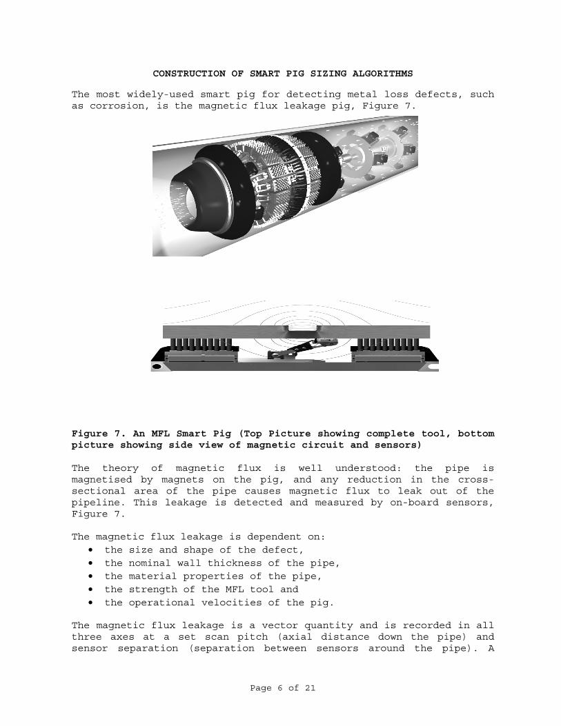
The most widely-used smart pig for detecting metal loss defects, such as corrosion, is the magnetic flux leakage pig, Figure 7.

Figure 7. An MFL Smart Pig (Top Picture showing complete tool, bottom picture showing side view of magnetic circuit and sensors) The theory of magnetic flux is well understood: the pipe is magnetised by magnets on the pig, and any reduction in the cross-sectional area of the pipe causes magnetic flux to leak out of the pipeline. This leakage is detected and measured by on-board sensors, Figure 7. The magnetic flux leakage is dependent on:

• the size and shape of the defect, • the nominal wall thickness of the pipe, • the material properties of the pipe, • the strength of the MFL tool and • the operational velocities of the pig.

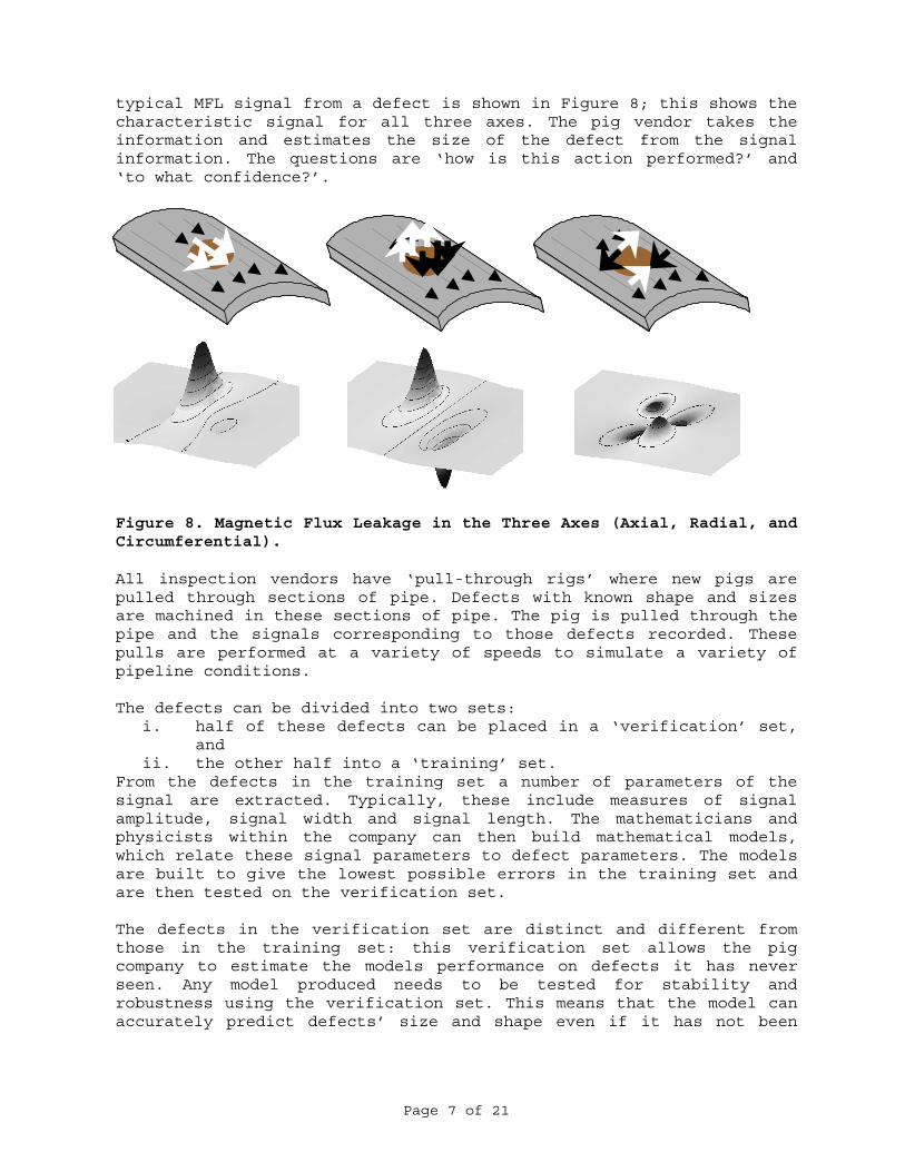
The magnetic flux leakage is a vector quantity and is recorded in all three axes at a set scan pitch (axial distance down the pipe) and sensor separation (separation between sensors around the pipe). A

Page 7 of 21

typical MFL signal from a defect is shown in Figure 8; this shows the characteristic signal for all three axes. The pig vendor takes the information and estimates the size of the defect from the signal information. The questions are ‘how is this action performed?’ and ‘to what confidence?’.

Figure 8. Magnetic Flux Leakage in the Three Axes (Axial, Radial, and Circumferential). All inspection vendors have ‘pull-through rigs’ where new pigs are pulled through sections of pipe. Defects with known shape and sizes are machined in these sections of pipe. The pig is pulled through the pipe and the signals corresponding to those defects recorded. These pulls are performed at a variety of speeds to simulate a variety of pipeline conditions. The defects can be divided into two sets:

i. half of these defects can be placed in a ‘verification’ set, and

ii. the other half into a ‘training’ set. From the defects in the training set a number of parameters of the signal are extracted. Typically, these include measures of signal amplitude, signal width and signal length. The mathematicians and physicists within the company can then build mathematical models, which relate these signal parameters to defect parameters. The models are built to give the lowest possible errors in the training set and are then tested on the verification set. The defects in the verification set are distinct and different from those in the training set: this verification set allows the pig company to estimate the models performance on defects it has never seen. Any model produced needs to be tested for stability and robustness using the verification set. This means that the model can accurately predict defects’ size and shape even if it has not been

Page 8 of 21

trained on the data. Ultimately, it is the result of the verification set that determines whether a model is selected.

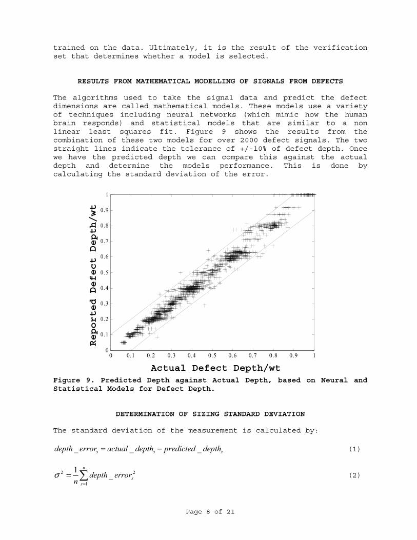
RESULTS FROM MATHEMATICAL MODELLING OF SIGNALS FROM DEFECTS The algorithms used to take the signal data and predict the defect dimensions are called mathematical models. These models use a variety of techniques including neural networks (which mimic how the human brain responds) and statistical models that are similar to a non linear least squares fit. Figure 9 shows the results from the combination of these two models for over 2000 defect signals. The two straight lines indicate the tolerance of +/-10% of defect depth. Once we have the predicted depth we can compare this against the actual depth and determine the models performance. This is done by calculating the standard deviation of the error.

Figure 9. Predicted Depth against Actual Depth, based on Neural and Statistical Models for Defect Depth.

DETERMINATION OF SIZING STANDARD DEVIATION The standard deviation of the measurement is calculated by:

sss depthpredicteddepthactualerrordepth ___ −= (1)

∑=

=n

sserrordepth

n 1

22 _1σ (2)

0 0.1 0.2 0.3 0.4 0.5 0.6 0.7 0.8 0.9 10

0.1

0.2

0.3

0.4

0.5

0.6

0.7

0.8

0.9

1

Actual Defect Depth/wt

Reported Defect Depth/wt

Page 9 of 21

where n is the total number of defects and σ is the standard deviation of the error. Figure 10 shows the distribution of the depth error for the previous data, assuming that this distribution is normal in nature.

-0.2 -0.15 -0.1 -0.05 0 0.05 0.1 0.15 0.20

50

100

150

200

250

300

350

Error in Depth Measurement (% Wall Loss)

NumberofDefects

Figure 10. The Distribution of Errors in Depth (based on Figure 9 data).

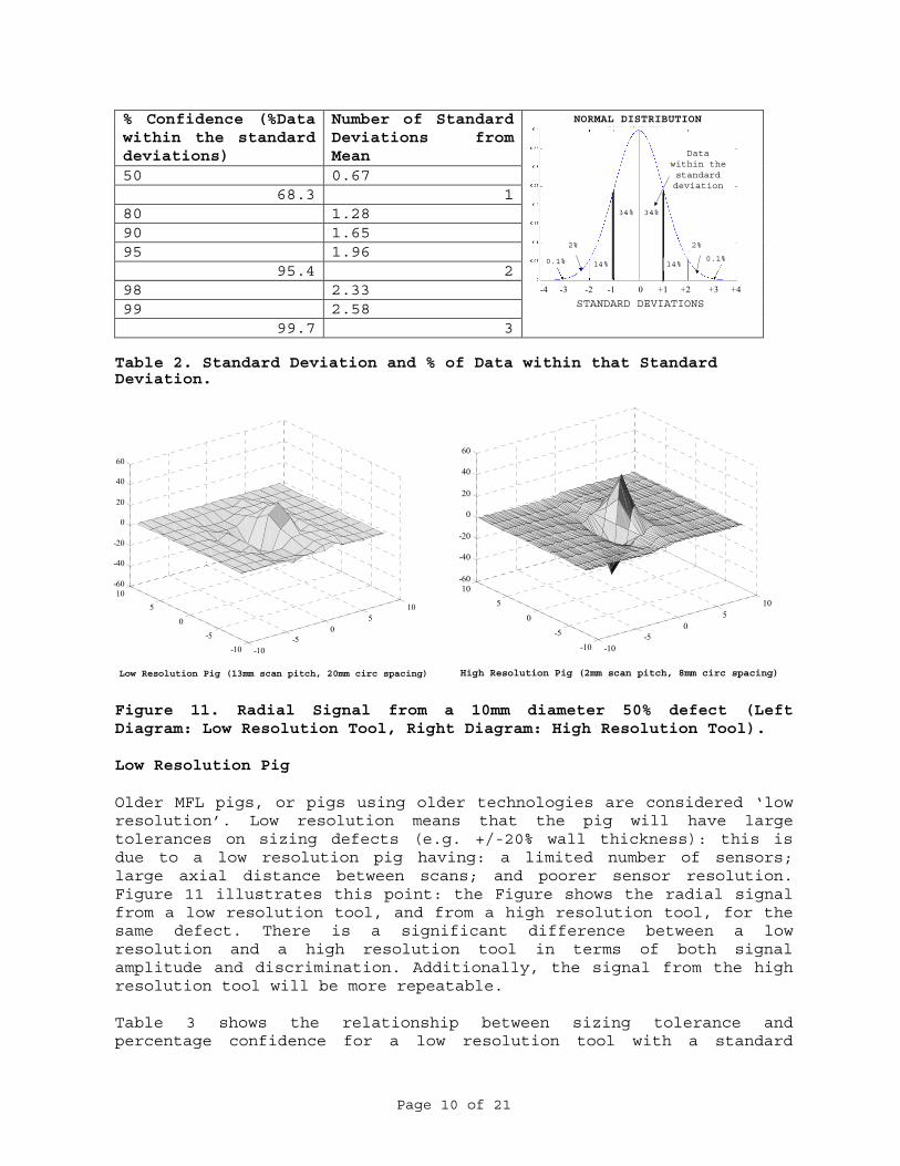
STANDARD DEVIATION AND SIZING TOLERANCE From simple statistics we can relate the standard deviation in Equation 2 to a sizing tolerance and confidence. Table 2 shows the percentage of data within a variety of standard deviations: for example, 68.3% of the probable data values lie within one (±) standard deviation of the reported value. Increasing the number of standard deviations increases the likelihood that the true vale is within that range(2); for example, adding and subtracting three standard deviations onto a measurement means that the true value of the measurement will only exceed that range 0.25% of the time. Table 2 can be used with defect depth sizing: a defect that has been sized at 50% deep with a standard deviation of 7.8% wall thickness implies that the true depth is within the range 26.6% (i.e. 50% -(3x7.8%) and 73.4% (i.e. 50%+(3x7.8%)), 997 times out of a 1000 (3 standard deviations).

2 The confidence level indicates the portion of measurements that will fall within a given sizing accuracy.

Number of

Defects

Error in Depth Measurement (defect depth/wt)

Page 10 of 21

% Confidence (%Data within the standard deviations)

Number of Standard Deviations from Mean

50 0.67 68.3 1

80 1.28 90 1.65 95 1.96

95.4 298 2.33 99 2.58

99.7 3

Table 2. Standard Deviation and % of Data within that Standard Deviation.

Figure 11. Radial Signal from a 10mm diameter 50% defect (Left Diagram: Low Resolution Tool, Right Diagram: High Resolution Tool). Low Resolution Pig Older MFL pigs, or pigs using older technologies are considered ‘low resolution’. Low resolution means that the pig will have large tolerances on sizing defects (e.g. +/-20% wall thickness): this is due to a low resolution pig having: a limited number of sensors; large axial distance between scans; and poorer sensor resolution. Figure 11 illustrates this point: the Figure shows the radial signal from a low resolution tool, and from a high resolution tool, for the same defect. There is a significant difference between a low resolution and a high resolution tool in terms of both signal amplitude and discrimination. Additionally, the signal from the high resolution tool will be more repeatable. Table 3 shows the relationship between sizing tolerance and percentage confidence for a low resolution tool with a standard

-10-5

05

10

-10-5

0

510

-60

-40

-20

0

20

40

60

High Resolution Pig (2mm scan pitch, 8mm circ spacing)

-10-5

05

10

-10-5

0

510

-60

-40

-20

0

20

40

60

Low Resolution Pig (13mm scan pitch, 20mm circ spacing)

0.1% 0.1%

34% 34%

14% 14%

2% 2%

-4 -3 0-2 -1 +1 +2 +3 +4STANDARD DEVIATIONS

Data within the standard deviation

NORMAL DISTRIBUTION

Page 11 of 21

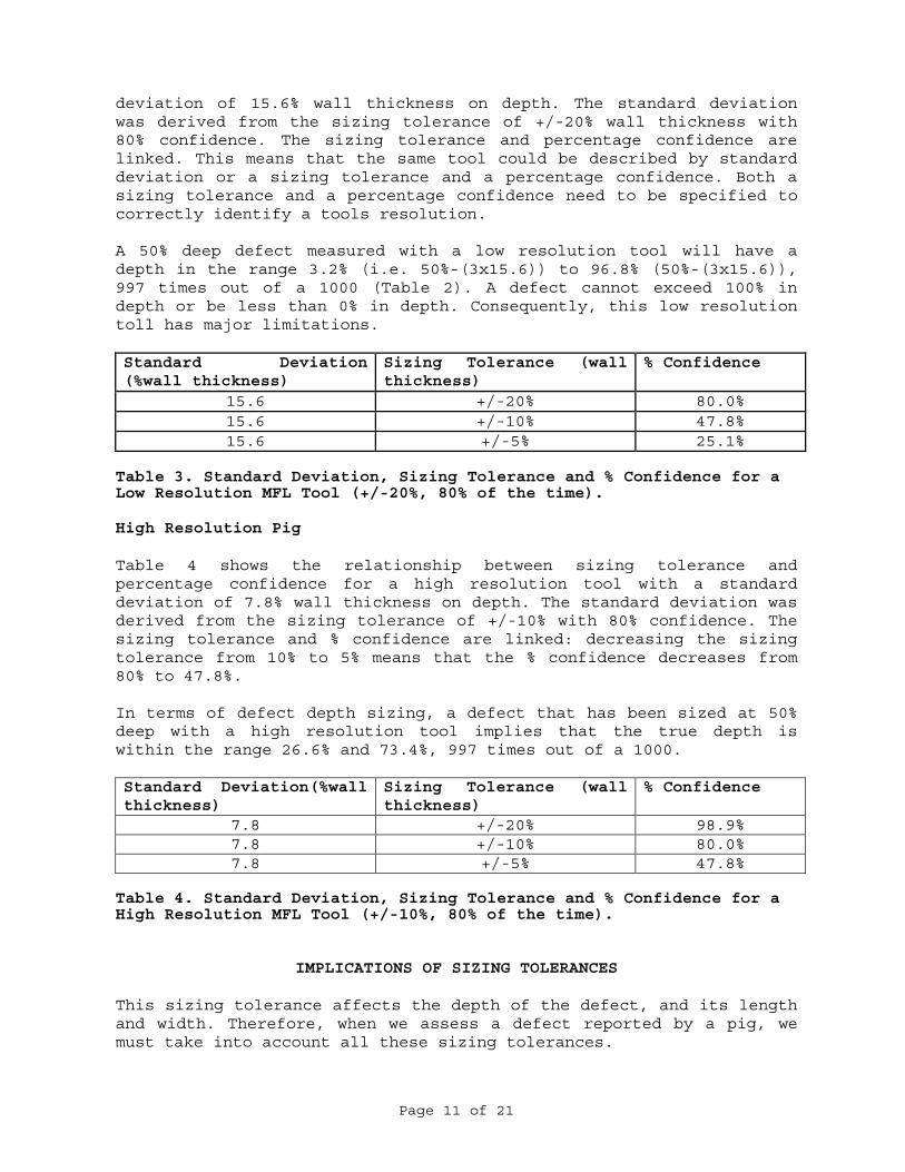
deviation of 15.6% wall thickness on depth. The standard deviation was derived from the sizing tolerance of +/-20% wall thickness with 80% confidence. The sizing tolerance and percentage confidence are linked. This means that the same tool could be described by standard deviation or a sizing tolerance and a percentage confidence. Both a sizing tolerance and a percentage confidence need to be specified to correctly identify a tools resolution. A 50% deep defect measured with a low resolution tool will have a depth in the range 3.2% (i.e. 50%-(3x15.6)) to 96.8% (50%-(3x15.6)), 997 times out of a 1000 (Table 2). A defect cannot exceed 100% in depth or be less than 0% in depth. Consequently, this low resolution toll has major limitations. Standard Deviation (%wall thickness)

Sizing Tolerance (wall thickness)

% Confidence

15.6 +/-20% 80.0% 15.6 +/-10% 47.8% 15.6 +/-5% 25.1%

Table 3. Standard Deviation, Sizing Tolerance and % Confidence for a Low Resolution MFL Tool (+/-20%, 80% of the time). High Resolution Pig Table 4 shows the relationship between sizing tolerance and percentage confidence for a high resolution tool with a standard deviation of 7.8% wall thickness on depth. The standard deviation was derived from the sizing tolerance of +/-10% with 80% confidence. The sizing tolerance and % confidence are linked: decreasing the sizing tolerance from 10% to 5% means that the % confidence decreases from 80% to 47.8%. In terms of defect depth sizing, a defect that has been sized at 50% deep with a high resolution tool implies that the true depth is within the range 26.6% and 73.4%, 997 times out of a 1000. Standard Deviation(%wall thickness)

Sizing Tolerance (wall thickness)

% Confidence

7.8 +/-20% 98.9% 7.8 +/-10% 80.0% 7.8 +/-5% 47.8%

Table 4. Standard Deviation, Sizing Tolerance and % Confidence for a High Resolution MFL Tool (+/-10%, 80% of the time).

IMPLICATIONS OF SIZING TOLERANCES This sizing tolerance affects the depth of the defect, and its length and width. Therefore, when we assess a defect reported by a pig, we must take into account all these sizing tolerances.

Page 12 of 21

This section discusses and illustrates how we can include these tolerances in our defect assessments. Calculating the Failure Pressure of Pipeline Defects When a defect is detected in a pipeline, the operator will want to know if the defect will cause a failure, or requires repair. Therefore, the failure pressure of the defective section of pipe needs to be calculated: if its failure pressure is below the maximum allowable operating pressure of the pipeline, it will require repair. There are many methods available to calculate the failure pressure of defects in pipelines4-11. Figure 2 shows ASME B31G6: this document allows an acceptance curve to be drawn. Any defect size that falls below the curve in Figure 2 is unacceptable, and will require remedial actions. Uncertainties in Failure Calculations There are four major ‘errors’ (better described as uncertainties, or lack of knowledge) associated with a defect assessment:

i. Defect equations modelling error: • All defect failure models will have modelling uncertainty

(see later Section). • All failure equations (Refs 4-11) will have an associated

uncertainty. This uncertainty is usually accommodated by applying a large, single safety factor to the failure calculation.

ii. Defect sizing errors: • Historically, sizing errors have been small; most defects

were measured directly, ‘in the ditch’. The use of pigs now requires these uncertainties to be accounted for.

iii. Operational uncertainties (pressure surges, human error, etc.):

• Operational uncertainties can usually be reduced by good pipeline engineering and management practices,

iv. Material variations (geometry, tensile properties, etc.): • Variations in material and geometry properties are

accommodated by using lower bound, reliable design data that will not give excessive errors (e.g. using specified diameter, SMYS, etc.),

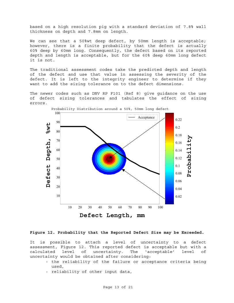
Including Defect Sizing Tolerances in Failure Calculations As discussed above, we must consider the errors associated with the reported defect. Figure 12 shows a defect reported as 50%wt deep, by 50mm in length. Figure 12 assesses this defect against the defect acceptance criterion in DNV RP F1018. Also plotted on this Figure are the probabilities of it being another size: these probabilities are

Page 13 of 21

based on a high resolution pig with a standard deviation of 7.8% wall thickness on depth and 7.8mm on length. We can see that a 50%wt deep defect, by 50mm length is acceptable; however, there is a finite probability that the defect is actually 60% deep by 60mm long. Consequently, the defect based on its reported depth and length is acceptable, but for the 60% deep 60mm long defect it is not. The traditional assessment codes take the predicted depth and length of the defect and use that value in assessing the severity of the defect. It is left to the integrity engineer to determine if they want to add the sizing tolerance on to the defect dimensions. The newer codes such as DNV RP F101 (Ref 8) give guidance on the use of defect sizing tolerances and tabulates the effect of sizing errors.

Figure 12. Probability that the Reported Defect Size may be Exceeded. It is possible to attach a level of uncertainty to a defect assessment, Figure 12. This reported defect is acceptable but with a calculated level of uncertainty. The ‘acceptable’ level of uncertainty would be obtained after considering:

- the reliability of the failure or acceptance criteria being used,

- reliability of other input data,

10 20 30 40 50 60 70 80 90 100

10

20

30

40

50

60

70

80

90

100

Defect Length (mm)

Def

ect D

epth

(%)

Probability Distribution around a 50%, 50mm long defect

0.02

0.04

0.06

0.08

0.1

0.12

0.14

0.16

0.18

0.2

0.22Acceptance

Defect Length, mm

Defect Depth, %wt

Probability

Page 14 of 21

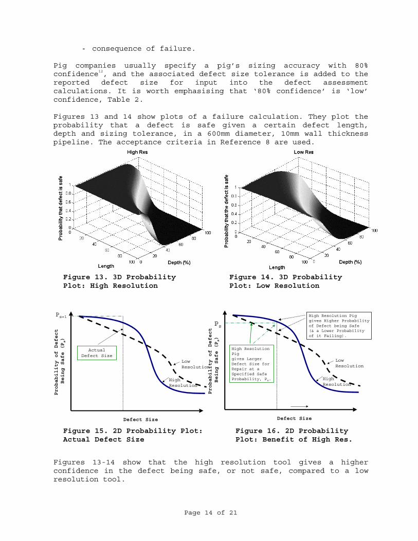
- consequence of failure. Pig companies usually specify a pig’s sizing accuracy with 80% confidence12, and the associated defect size tolerance is added to the reported defect size for input into the defect assessment calculations. It is worth emphasising that ‘80% confidence’ is ‘low’ confidence, Table 2. Figures 13 and 14 show plots of a failure calculation. They plot the probability that a defect is safe given a certain defect length, depth and sizing tolerance, in a 600mm diameter, 10mm wall thickness pipeline. The acceptance criteria in Reference 8 are used.

Figures 13-14 show that the high resolution tool gives a higher confidence in the defect being safe, or not safe, compared to a low resolution tool.

Figure 13. 3D Probability Plot: High Resolution

Figure 14. 3D Probability Plot: Low Resolution

Ps=1

Actual Defect Size

Low Resolution

HighResolution

Probability of Defect

Being Safe (Ps)

Defect Size

Figure 16. 2D Probability Plot: Benefit of High Res.

Ps

High Resolution Piggives Higher Probabilityof Defect being Safe (& a Lower Probability of it Failing).

Low Resolution

HighResolution

High Resolution Piggives Larger Defect Size for Repair at a Specified Safe Probability, Ps.

Probability of Defect

Being Safe (Ps)

Defect Size

Figure 15. 2D Probability Plot: Actual Defect Size

Page 15 of 21

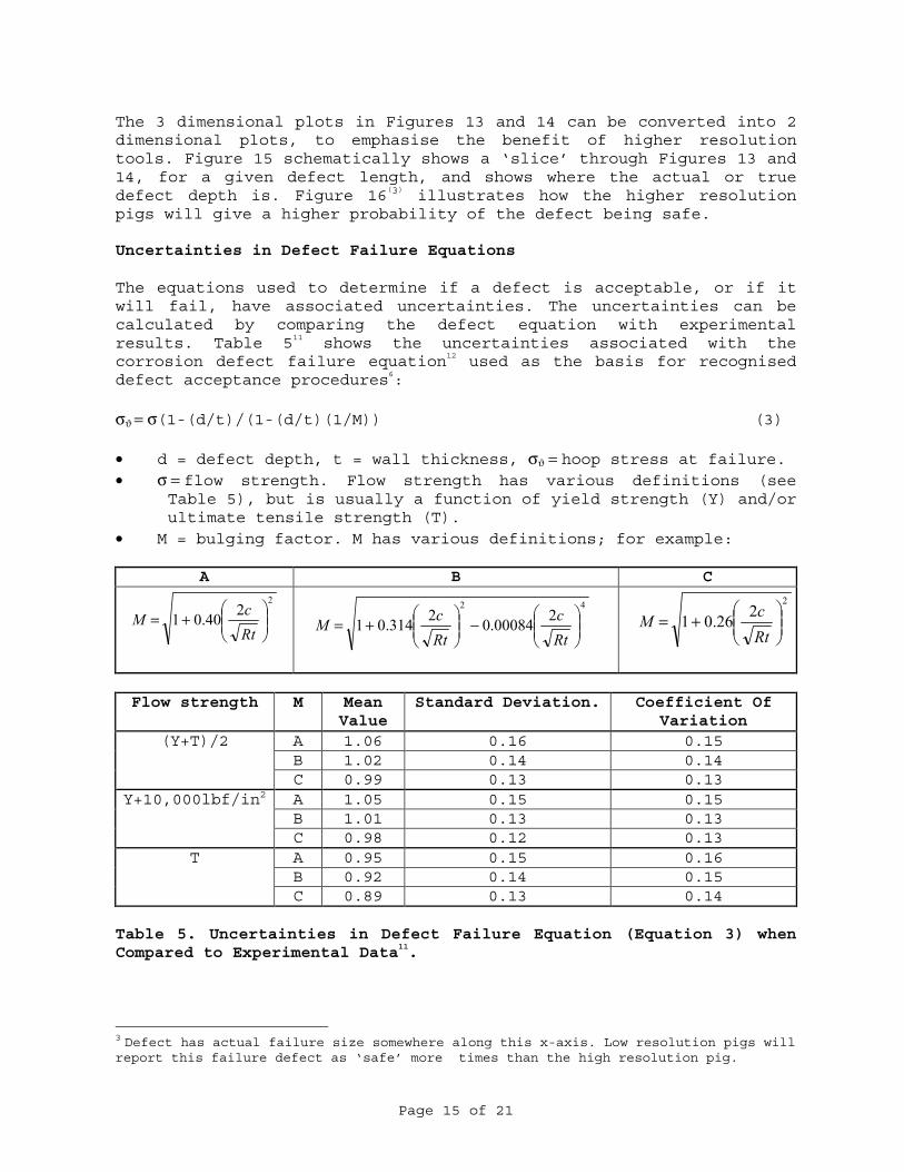
The 3 dimensional plots in Figures 13 and 14 can be converted into 2 dimensional plots, to emphasise the benefit of higher resolution tools. Figure 15 schematically shows a ‘slice’ through Figures 13 and 14, for a given defect length, and shows where the actual or true defect depth is. Figure 16(3) illustrates how the higher resolution pigs will give a higher probability of the defect being safe. Uncertainties in Defect Failure Equations The equations used to determine if a defect is acceptable, or if it will fail, have associated uncertainties. The uncertainties can be calculated by comparing the defect equation with experimental results. Table 511 shows the uncertainties associated with the corrosion defect failure equation12 used as the basis for recognised defect acceptance procedures6: σϑ = σ(1-(d/t)/(1-(d/t)(1/M)) (3) • d = defect depth, t = wall thickness, σϑ = hoop stress at failure. • σ = flow strength. Flow strength has various definitions (see

Table 5), but is usually a function of yield strength (Y) and/or ultimate tensile strength (T).

• M = bulging factor. M has various definitions; for example:

A B C

Flow strength M Mean

Value Standard Deviation. Coefficient Of

Variation A 1.06 0.16 0.15 B 1.02 0.14 0.14

(Y+T)/2

C 0.99 0.13 0.13 A 1.05 0.15 0.15 B 1.01 0.13 0.13

Y+10,000lbf/in2

C 0.98 0.12 0.13 A 0.95 0.15 0.16 B 0.92 0.14 0.15

T

C 0.89 0.13 0.14 Table 5. Uncertainties in Defect Failure Equation (Equation 3) when Compared to Experimental Data11.

3 Defect has actual failure size somewhere along this x-axis. Low resolution pigs will report this failure defect as ‘safe’ more times than the high resolution pig.

42200084.02314.01

−

+=

Rtc

RtcM

2240.01

+=

RtcM

2226.01

+=

RtcM

Page 16 of 21

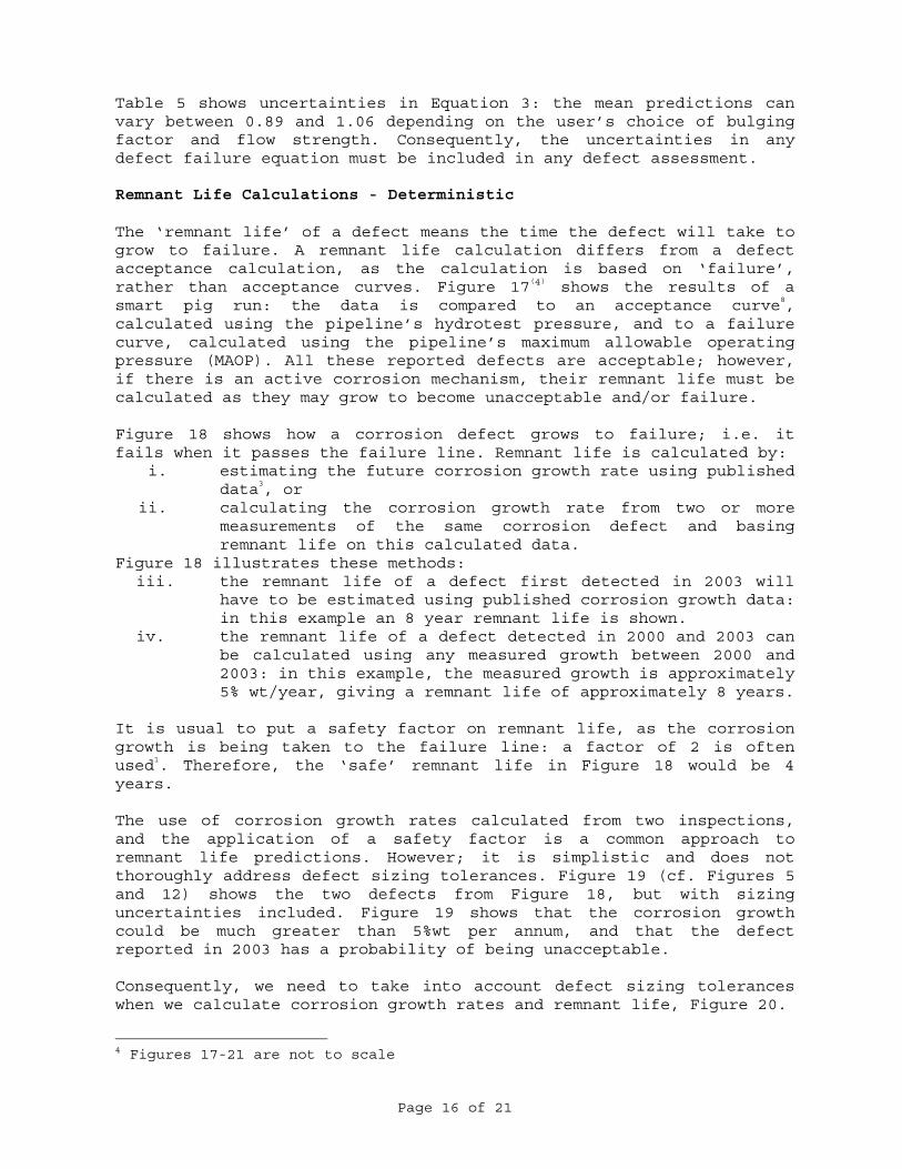
Table 5 shows uncertainties in Equation 3: the mean predictions can vary between 0.89 and 1.06 depending on the user’s choice of bulging factor and flow strength. Consequently, the uncertainties in any defect failure equation must be included in any defect assessment. Remnant Life Calculations - Deterministic The ‘remnant life’ of a defect means the time the defect will take to grow to failure. A remnant life calculation differs from a defect acceptance calculation, as the calculation is based on ‘failure’, rather than acceptance curves. Figure 17(4) shows the results of a smart pig run: the data is compared to an acceptance curve8, calculated using the pipeline’s hydrotest pressure, and to a failure curve, calculated using the pipeline’s maximum allowable operating pressure (MAOP). All these reported defects are acceptable; however, if there is an active corrosion mechanism, their remnant life must be calculated as they may grow to become unacceptable and/or failure. Figure 18 shows how a corrosion defect grows to failure; i.e. it fails when it passes the failure line. Remnant life is calculated by:

i. estimating the future corrosion growth rate using published data3, or

ii. calculating the corrosion growth rate from two or more measurements of the same corrosion defect and basing remnant life on this calculated data.

Figure 18 illustrates these methods: iii. the remnant life of a defect first detected in 2003 will

have to be estimated using published corrosion growth data: in this example an 8 year remnant life is shown.

iv. the remnant life of a defect detected in 2000 and 2003 can be calculated using any measured growth between 2000 and 2003: in this example, the measured growth is approximately 5% wt/year, giving a remnant life of approximately 8 years.

It is usual to put a safety factor on remnant life, as the corrosion growth is being taken to the failure line: a factor of 2 is often used1. Therefore, the ‘safe’ remnant life in Figure 18 would be 4 years. The use of corrosion growth rates calculated from two inspections, and the application of a safety factor is a common approach to remnant life predictions. However; it is simplistic and does not thoroughly address defect sizing tolerances. Figure 19 (cf. Figures 5 and 12) shows the two defects from Figure 18, but with sizing uncertainties included. Figure 19 shows that the corrosion growth could be much greater than 5%wt per annum, and that the defect reported in 2003 has a probability of being unacceptable. Consequently, we need to take into account defect sizing tolerances when we calculate corrosion growth rates and remnant life, Figure 20.

4 Figures 17-21 are not to scale

Page 17 of 21

Figure 18. Defect Remnant Life

0.0

0.1

0.2

0.3

0.4

0.5

0.6

0.7

0.8

0.9

1.0

0 100 200 300 400 500 600 700 800 900 1000 1100 1200 1300 1400 1500 1600 1700 1800 1900 2000

Defect Length (mm)

Failure Line (MAOP)

Acceptance Line (Hydrotest)

Defect Length (mm)1000500 1500 2000


+ corrosion

Acceptable

Not Acceptable

No Failure

Failure

Figure 17. Defect ‘Acceptance’ and ‘Failure’


0.0

0.1

0.2

0.3

0.4

0.5

0.6

0.7

0.8

0.9

1.0

0 500 600 700 800 900 1000 1100 1200 1300 1400 1500 1600 1700 1800 1900 2000

Defect Length (mm)

Failure Line (MAOP)



No Failure

Failure

2000 Inspection

2003 Inspection

Remnant Life:

8 years to Failure

Corrosion Growth Rate

calculated from these sizes

Figure 19. Defect Measurement Uncertainties Figure 20. Growth Rate and Remnant Life Uncertainties

0.0

0.1

0.2

0.3

0.4

0.5

0.6

0.7

0.8

0.9

1.0

0 500 600 700 800 900 1000 1100 1200 1300 1400 1500 1600 1700 1800 1900 2000

Defect Length (mm)

Failure Line (MAOP)




2000 Inspection

2003 Inspection

Remnant Life:

8 years to Failure with a probability

0.0

0.1

0.2

0.3

0.4

0.5

0.6

0.7

0.8

0.9

1.0

0 500 600 700 800 900 1000 1100 1200 1300 1400 1500 1600 1700 1800 1900 2000

Defect Length (mm)

Failure Line (MAOP)




Remnant Life:

Time & Probability

Corrosion Growth Rate:

Rate & Probability

Page 18 of 21

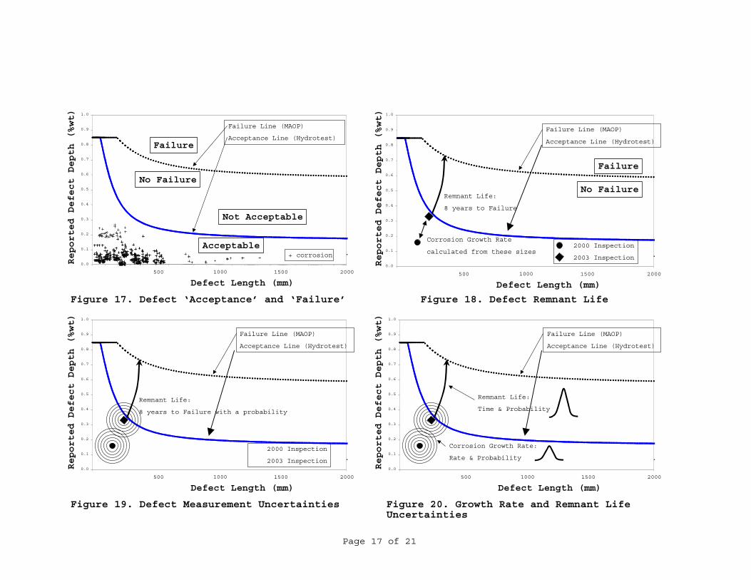
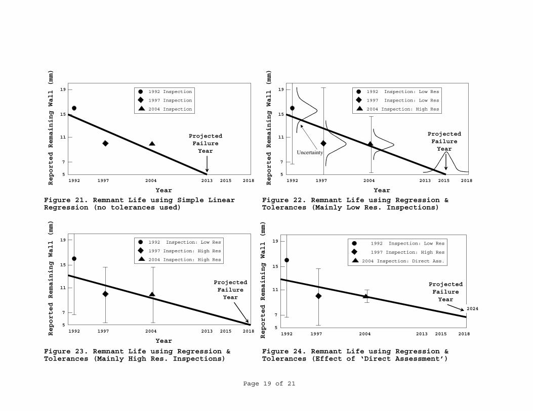
Remnant Life Calculations – Taking Account of Tolerances Figures 18 and 21 present a simple method for calculating remnant life for a corrosion defect using deterministic methods. Corrosion growth is calculated from inspections on the same defect: simple linear regression(5) can be used to calculate a corrosion growth rate, and this rate used to determine the remnant life: Figure 21(6) uses three measurements of a defect to estimate a linear corrosion growth rate. This rate is then used to predict when the defect will fail the pipeline. In this example, the failure occurs when the defect grows to a depth with a remaining wall thickness of 5mm, and failure is predicted in 2013. The same plot would be obtained if the same pig with the same tolerances and same confidence levels were used (e.g. +/-2mm, 80% of the time) in each of the three years. As discussed above, Figure 21 is simplistic: it takes no account of the tolerances associated with differing tools and sizing methods. The corrosion growth rate must be calculated using the sizing tolerances and uncertainties, Figure 22. This is not a simple exercise as it involves calculating the growth rates from a number of defect sizes and associated tolerances and uncertainties. Figures 22-24 (Table 6) show the remnant life calculation, but differing methods and pigs are used, and tolerances are included:

FIGURE 22: INSPECTION TOOL TOLERANCE

(+/-%wt) Confidence Level (%)

Predicted Failure Year

1992 Low Res Pig 20 80 1997 Low Res Pig 20 80 2004 High Res Pig 10 80

2015




1992 Low Res Pig 20 80 1997 High Res Pig 10 80 2004 High Res Pig 10 80

2018




1992 Low Res Pig 20 80 1997 High Res Pig 10 80 2004 Wall

thickness probe

2.5 90 2024

Table 6. Effect of Differing Tools and Tolerances on Remnant Life Predictions.

5 Corrosion is assumed to grow linearly with time in Figures 21-24. Other growth patterns can be used if more appropriate. 6 Figures 21-24 are not to scale.

Page 19 of 21

Figure 21. Remnant Life using Simple Linear Regression (no tolerances used)

Figure 22. Remnant Life using Regression & Tolerances (Mainly Low Res. Inspections)

Figure 24. Remnant Life using Regression & Tolerances (Effect of ‘Direct Assessment’)

Figure 23. Remnant Life using Regression & Tolerances (Mainly High Res. Inspections)

19

11

15

7

5

1992 Inspection

1997 Inspection

2004 Inspection

Reported Remaining Wall (mm)

Year

1992 1997 2004 2013 2018

ProjectedFailureYear

2015

19

11

15

7

5


Year

1992 Inspection: Low Res

1997 Inspection: High Res



1992 1997 2004 201820152013

19

11

15

7

5




2004 Inspection: Direct Ass.


2024

1992 1997 2004 201820152013

19

11

15

7

5


Year




ProjectedFailureYearUncertainty

1992 1997 2004 201820152013

Page 20 of 21

Figures 22-24 assume that failure occurs when the remaining wall thickness below the defect is 5mm. It is easy to perform the linear regression in Figure 21, but Figures 22-24 draw the corrosion growth line through the reported defect sizes, taking into account the confidence levels in Table 6: these are not simple calculations. Figures 21-24 show:

i. Using higher resolution tools can give a higher confidence in projected corrosion rates. This can result in longer remnant life predictions.

ii. Figure 24 clearly shows the benefit of accurate defect sizing: in this Figure, it is assumed that the defect is measured directly (‘direct assessment’) using a hand held ultrasonic wall thickness probe. The high confidence associated with this measurement is reflected in the longer projected remnant life.

iii. All the projections in these Figures need an additional analysis: they need an estimate of the probability of failure at future years, Figure 22 (see next), rather than the simple projections highlighted in the Figures.

Finally it should be noted that Figures 21-24 show high resolution inspections to give higher confidence in remnant life predictions, but lower resolution inspections should not be dismissed: all inspections have value. The operator must decide on the most effective inspection method for their pipeline Remnant Life Calculations – Probabilistic A full probabilistic calculation on the inspection results in Figures 22-24, can be conducted to ensure that all possible corrosion growth rates are assessed, and this would give a probability of failure curve at each future year, Figure 22, rather than the simple deterministic projections in the Figures. These probabilistic methods will be published in a future paper13. The calculations in Figures 21-24 can additionally include the failure equation modelling error (Table 5), and any other uncertainty in input data to give an accurate probability of failure for any defect.

SUMMARY This paper has shown how defect sizing tolerances are calculated by pigging companies and used in both defect assessments and remnant life calculations for corrosion defects. It is important to take account of the reported tolerances, particularly when projecting corrosion growth using pig data.

Page 21 of 21

REFERENCES 1. ‘Managing System Integrity for Hazardous Liquid Lines’, 1st Ed.,

ANSI/ASME Standard 1160-2001, November 2001. 2. US Department of Transportation. Federal Register Parts 49 CFR

195.452 (May 2001) and Part 49 CFR 192.763. (January 2003). 3. ‘Managing System Integrity of Gas Pipelines’, ASME B31.8S 2001.

Supplement to ASME B31.8, ASME International, New York, USA. 4. Kiefner, J. F., Maxey, W. A., Eiber, R. J., and Duffy, A. R.,

‘The Failure Stress Levels of Flaws in Pressurised Cylinders’, ASTM STP 536, American Society for Testing and Materials, Philadelphia, pp. 461-481. 1973.

5. Kiefner, J. F., Vieth, P. H., ‘A Modified Criterion for Evaluating the Strength of Corroded Pipe’, Final Report for Project PR 3-805 to the Pipeline Supervisory Committee of the American Gas Association, Battelle, Ohio. 1989.

6. ‘Manual for Determining the Remaining Strength of Corroded Pipelines’, A Supplement to ASME B31 Code for Pressure Piping, ASME B31G-1991 (Revision of ANSI/ASME B31G-1984), The American Society of Mechanical Engineers, New York, USA, 1991.

7. Kiefner, J. F., Vieth, P. H., and Roytman, I., ‘Continued Validation of RSTRENG’, Updated Draft Final Report on Contract No. PR 218-9304 to Line Pipe Research Supervisory Committee, Pipeline Research Committee of the American Gas Association, Kiefner and Associates, Inc. 1995.

8. ‘Corroded Pipelines’, DNV-RP-F101. Det Norske Veritas, 1999. 9. ‘Guide on Methods for Assessing the Acceptability of Flaws in

Fusion Welded Structures’, BS 7910: Incorporating Amendment No. 1, British Standards Institution, London, UK, 1999.

10. ‘Fitness-For-Service’, API Recommended Practice 579, First Edition. American Petroleum Institute, January 2000.

11. Cosham, A, Hopkins, P., ‘The Pipeline Defect Assessment Manual’, IPC 2002: International Pipeline Conference, Calgary, Alberta, Canada, October 2002.

12. ‘Specifications and Requirements for Intelligent Pig Inspection of Pipelines’, Pipeline Operators’ Forum (POF). Version 2.1, 6 November 1998.

13. Turner, S, Wickham, A. To be published 2004.

Documents

This document was downloaded from the Penspen Integrity ... · 4839 90th Avenue S.E Calgary, Alberta Canada Phil Hopkins Penspen Ltd. Hawthorn Suite St. Peter’s Wharf Newcastle