Embed Size (px)
Citation preview

Dis
sert
atio
nsr
eih
e Ph
ysik
- B
and
47
A Semiclassical Approach to Many-Body Interference in Fock-Space
Thomas Engl
479 783868 451283
ISBN 978-3-86845-128-3Th
om
as E
ng
lISBN 978-3-86845-128-3
Many-body systems draw ever more physicists’ attention. Such an increase of interest often comes along with the development of new theoretical methods. In this thesis, a non-perturbative semiclassical approach is developed, which allows to analytically study many-body interference effects both in bosonic and fermionic Fock space and is expected to be applicable to many research areas in physics ranging from Quantum Optics and Ultracold Atoms to Solid State Theory and maybe even High Energy Physics.After the derivation of the semiclassical approximation, which is valid in the limit of large total number of particles, first applications manifesting the presence of many-body interference effects are shown. Some of them are confirmed numerically thus verifying the semiclassical predictions. Among these results are coherent back-/forward-scattering in bosonic and fermionic Fock space as well as a many-body spin echo, to name only the two most important ones.

Thomas Engl
A Semiclassical Approach toMany-Body Interference in Fock-Space

Herausgegeben vom Präsidium des Alumnivereins der Physikalischen Fakultät:Klaus Richter, Andreas Schäfer, Werner Wegscheider, Dieter Weiss
Dissertationsreihe der Fakultät für Physik der Universität Regensburg, Band 47
A Semiclassical Approach to Many-Body Interference in Fock-Space Dissertation zur Erlangung des Doktorgrades der Naturwissenschaften (Dr. rer. nat.)der naturwissenschaftlichen Fakultät II - Physik der Universität Regensburgvorgelegt von
Thomas Engl
aus Rodingim Juni 2015
Promotionsgesuch eingereicht am: 10.06.2014Die Arbeit wurde angeleitet von: Prof. Dr. Klaus Richter
Prüfungsausschuss: Vorsitzender: Prof. Dr. Rupert Huber
1. Gutachter: Prof. Dr. Klaus Richter
2. Gutachter: Prof. Dr. Milena Grifoni
weiterer Prüfer: Prof. Dr. Andreas Schäfer

Thomas EnglA Semiclassical Approach toMany-Body Interference in Fock-Space

Bibliografische Informationen der Deutschen Bibliothek.Die Deutsche Bibliothek verzeichnet diese Publikationin der Deutschen Nationalbibliografie. Detailierte bibliografische Daten sind im Internet über http://dnb.ddb.de abrufbar.
1. Auflage 2015© 2015 Universitätsverlag, RegensburgLeibnizstraße 13, 93055 Regensburg
Konzeption: Thomas Geiger Umschlagentwurf: Franz Stadler, Designcooperative Nittenau eGLayout: Thomas Engl Druck: Docupoint, MagdeburgISBN: 978-3-86845-128-3
Alle Rechte vorbehalten. Ohne ausdrückliche Genehmigung des Verlags ist es nicht gestattet, dieses Buch oder Teile daraus auf fototechnischem oder elektronischem Weg zu vervielfältigen.
Weitere Informationen zum Verlagsprogramm erhalten Sie unter:www.univerlag-regensburg.de

A Semiclassical Approach toMany-Body Interference in
Fock-Space
DISSERTATIONZUR ERLANGUNG DES DOKTORGRADES
DER NATRUWISSENSCHAFTEN (DR. RER. NAT.)DER FAKULTAT FUR PHYSIK
DER UNIVERSITAT REGENSBURG
vorgelegt von
Thomas Engl
aus
Roding
im Jahr 2015

Promotionsgesuch eingereicht am: 10.06.2014Die Arbeit wurde angeleitet von: Prof. Dr. Klaus Richter
Prufungsausschuss: Vorsitzender: Prof. Dr. Rupert Huber1. Gutachter: Prof. Dr. Klaus Richter2. Gutachter: Prof. Dr. Milena Grifoniweiterer Prufer: Prof. Dr. Andreas Schafer

Dedicated to Martin C. Gutzwiller


Contents
1 Introduction 11.1 Classical Mechanics gone Quantum . . . . . . . . . . . . . . 1
1.1.1 The first quantum revolution . . . . . . . . . . . . . 11.1.2 Second quantization . . . . . . . . . . . . . . . . . . 4
1.2 The Connection to Various Research Fields . . . . . . . . . 61.2.1 Quantum Optics . . . . . . . . . . . . . . . . . . . . 61.2.2 Ultra-cold Atoms in Optical Lattices . . . . . . . . . 71.2.3 Spintronics . . . . . . . . . . . . . . . . . . . . . . . 91.2.4 Many-Body effects in condensed matter physics . . . 101.2.5 Chemical Physics . . . . . . . . . . . . . . . . . . . . 11
1.3 Outline of this thesis . . . . . . . . . . . . . . . . . . . . . . 11
I Basic concepts 13
2 Semiclassics for Single-Particle Systems 152.1 The Path Integral Representation of the Propagator . . . . 15
2.1.1 The quantum mechanical propagator . . . . . . . . . 152.1.2 The Path integral . . . . . . . . . . . . . . . . . . . 18
2.2 The Semiclassical Approximation . . . . . . . . . . . . . . . 212.2.1 Stationary phase approximation . . . . . . . . . . . 212.2.2 The van-Vleck-Gutzwiller Propagator . . . . . . . . 23
2.3 Semiclassical Perturbation Theory . . . . . . . . . . . . . . 27
3 From Single- to Many-Body Physics: Second quantiza-tion and many-body states 313.1 Second Quantization and Fock states . . . . . . . . . . . . . 31
3.1.1 Bosonic creation and annihilation operators . . . . . 333.1.2 Fermionic creation and annihilation operators . . . . 353.1.3 Hamiltonian and observables in second quantization 37
vii
viii CONTENTS
3.2 Bosonic Many-Body States . . . . . . . . . . . . . . . . . . 38
3.2.1 Quadrature States . . . . . . . . . . . . . . . . . . . 38
3.2.2 Coherent States . . . . . . . . . . . . . . . . . . . . . 42
3.3 Fermionic Many-Body States . . . . . . . . . . . . . . . . . 43
3.3.1 Coherent States . . . . . . . . . . . . . . . . . . . . . 43
3.3.2 Klauder coherent states . . . . . . . . . . . . . . . . 45
II The Many-Body van-Vleck-Gutzwiller-Propagator inFock Space 47
4 Bosons 49
4.1 The semiclassical coherent state propagator . . . . . . . . . 49
4.2 The Quadrature Path Integral Representation . . . . . . . . 51
4.3 The Semiclassical Propagator in Quadrature Representation 54
4.3.1 Propagator between quadratures with the same phase 54
4.3.2 Propagator between quadratures with different phases 56
4.3.3 An initial value representation using quandratures . 57
4.4 The Semiclassical Propagator in Fock State Representation 59
4.4.1 The propagator . . . . . . . . . . . . . . . . . . . . . 59
4.4.2 The (approximate) semi-group property . . . . . . . 62
5 Fermions 67
5.1 The Propagator using Klauder’s Coherent State Represen-tation . . . . . . . . . . . . . . . . . . . . . . . . . . . . . . 68
5.1.1 The Path Integral . . . . . . . . . . . . . . . . . . . 68
5.1.2 Stationary phase approximation . . . . . . . . . . . 70
5.2 The Semiclassical Propagator in Fermionic Fock States . . . 72
5.2.1 The complex Path Integral for the Propagator inFock state Representation . . . . . . . . . . . . . . . 72
5.2.2 Semiclassical Approximation . . . . . . . . . . . . . 76
IIIInterference Effects in Bosonic Fock Space 83
6 Non-Interacting Systems 85
6.1 The Transition Probability for Quadratures . . . . . . . . . 85
6.1.1 The exact propagator in quadrature representation . 85
6.1.2 Propagation between quadratures with the same phase 87
6.1.3 Propagation between quadratures with different phase 89

CONTENTS ix
6.2 The Transition Probability in Coherent States . . . . . . . . 90
7 Many-Body Coherent Backscattering 95
7.1 Chaotic Regime . . . . . . . . . . . . . . . . . . . . . . . . . 95
7.1.1 Diagonal approximation . . . . . . . . . . . . . . . . 96
7.1.2 Coherent backscattering contribution . . . . . . . . . 97
7.1.3 Loop contributions . . . . . . . . . . . . . . . . . . . 101
7.2 Weak Coupling Regime . . . . . . . . . . . . . . . . . . . . 108
7.2.1 The propagator in quadrature representation for di-agonal Hamiltonians . . . . . . . . . . . . . . . . . . 109
7.2.2 Transition probability for weak hopping . . . . . . . 115
8 Many-Body Transport 119
8.1 Formulation of many-body transport . . . . . . . . . . . . . 119
8.2 Exact treatment of the leads . . . . . . . . . . . . . . . . . 121
8.3 Calculating Observables . . . . . . . . . . . . . . . . . . . . 125
8.3.1 A semiclassical formula for expectation values of single-particle observables . . . . . . . . . . . . . . . . . . . 125
8.3.2 Diagonal approximation: Rederiving the TruncatedWigner Approximation . . . . . . . . . . . . . . . . 128
8.3.3 Interference effects: Sieber-Richter Pairs and One-Leg-Loops . . . . . . . . . . . . . . . . . . . . . . . . 129
9 The fidelity for interacting bosonic many-body systems 133
9.1 The Fidelity Amplitude . . . . . . . . . . . . . . . . . . . . 133
9.1.1 Disordered system . . . . . . . . . . . . . . . . . . . 134
9.1.2 Short Time Behavior . . . . . . . . . . . . . . . . . . 136
9.2 The Loschmidt echo . . . . . . . . . . . . . . . . . . . . . . 137
9.2.1 Background contribution . . . . . . . . . . . . . . . 137
9.2.2 Incoherent contribution . . . . . . . . . . . . . . . . 138
9.2.3 Coherent contribution . . . . . . . . . . . . . . . . . 140
9.3 Discussion and comparison with numerical data . . . . . . . 142
9.3.1 Fidelity . . . . . . . . . . . . . . . . . . . . . . . . . 142
9.3.2 Loschmidt echo . . . . . . . . . . . . . . . . . . . . . 145
IVInterference Effects in Fermionic Fock Space 151
10 The Transition Probability for Fermionic Systems 153
10.1 Diagonal approximation . . . . . . . . . . . . . . . . . . . . 154

x CONTENTS
10.2 Coherent backscattering like contribution . . . . . . . . . . 155
10.3 Discussion . . . . . . . . . . . . . . . . . . . . . . . . . . . . 157
10.4 Further discrete symmetries . . . . . . . . . . . . . . . . . . 159
11 Many-Body Spin Echo 163
11.1 The spin-echo setup . . . . . . . . . . . . . . . . . . . . . . 163
11.2 Leading order contributions . . . . . . . . . . . . . . . . . . 166
11.3 No spin-flips: Semigroup property . . . . . . . . . . . . . . 170
11.4 Discussion of the results . . . . . . . . . . . . . . . . . . . . 172
11.5 Concluding remarks . . . . . . . . . . . . . . . . . . . . . . 173
11.5.1 Higher order contributions . . . . . . . . . . . . . . . 173
11.5.2 Incomplete spin flips . . . . . . . . . . . . . . . . . . 178
12 Many-Body Spin Fidelity 181
12.1 Unitarity . . . . . . . . . . . . . . . . . . . . . . . . . . . . 187
12.2 General Results . . . . . . . . . . . . . . . . . . . . . . . . . 188
12.2.1 Odd number of particles . . . . . . . . . . . . . . . . 188
12.2.2 Even number of particles . . . . . . . . . . . . . . . 189
13 Summary & Outlook 191
13.1 Summary . . . . . . . . . . . . . . . . . . . . . . . . . . . . 191
13.2 Outlook . . . . . . . . . . . . . . . . . . . . . . . . . . . . . 197
List of Publications 199
Acknowledgements 201
Appendix 205
A The Semiclassical Propagator for Bosons 205
A.1 The classical Hamiltonian for a Bose-Hubbard systems inquadrature representation . . . . . . . . . . . . . . . . . . . 205
A.2 The stationary phase approximation to the bosonic propa-gator in quadrature representation . . . . . . . . . . . . . . 208
A.3 The basis change from Quadratures to Fock states for thesemiclassical propagator . . . . . . . . . . . . . . . . . . . . 211
B The Feynman Path Integral for Fermions using complexvariables 219

CONTENTS xi
C Semiclassical propagator for Fermions 229C.1 Derivation of the semiclassical prefactor . . . . . . . . . . . 229C.2 Simplification of the semiclassical prefactor . . . . . . . . . 238
D The bosonic transition probability in the weak couplingregime 241D.1 Determination of the trajectory and its action . . . . . . . . 241D.2 Transformation to Fock states . . . . . . . . . . . . . . . . . 243
D.2.1 The coherent state propagator for weak hopping . . 245D.2.2 The propagator for weak hopping in number repre-
sentation . . . . . . . . . . . . . . . . . . . . . . . . 247
E Derivation of the propagator for open systems 249E.1 Splitting off the leads . . . . . . . . . . . . . . . . . . . . . 251E.2 The full propagator . . . . . . . . . . . . . . . . . . . . . . . 253E.3 Getting real actions and stationary phase approximation . . 255
F Loop contributions 259F.1 Two-leg-loops . . . . . . . . . . . . . . . . . . . . . . . . . . 260
F.1.1 Phase-space geometry . . . . . . . . . . . . . . . . . 260F.1.2 Partner trajectory . . . . . . . . . . . . . . . . . . . 263F.1.3 Existence . . . . . . . . . . . . . . . . . . . . . . . . 263F.1.4 Action difference . . . . . . . . . . . . . . . . . . . . 264F.1.5 Density of encounters . . . . . . . . . . . . . . . . . 266
F.2 One-leg-loops . . . . . . . . . . . . . . . . . . . . . . . . . . 268
G Hubbard-Stratonovich transformation 271
Bibliography 275


CHAPTER 1Introduction
1.1 Classical Mechanics gone Quantum
1.1.1 The first quantum revolution
100 years ago, not only the first world war broke out, but also JamesFranck and Gustav Hertz showed in their experiment that the electrons inan atom can have only certain quantized energies [1]. The Franck-Hertz ex-periment was the first experimental proof of the quantum nature of atoms,and also resulted in a Nobel prize for Franck and Hertz in 1925. At thattime, Bohr’s heuristic atom model [2], which in a way could be consideredas the first semiclassical model since it used quantized but otherwise clas-sical orbits, was considered to be the correct theory to describe the innerstructure of atoms.
The Bohr-Sommerfeld quantization rule actually yielded the correctenergy levels for the hydrogen atom even including fine structure. However,although many physicists – among them Bohr, Born, Kramers, Lande ,Sommerfeld and van Vleck – tried to compute it, the correct ground stateenergy of Helium could not be reproduced [3].
This failure to compute the energy levels of Helium marked the end ofthe “old quantum theory”. Finally, in 1925, works by Louis de Broglie,Werner Heisenberg and Erwin Schrodinger culminated in the Schrodingerequation [4]. A test of the thus developed “new quantum theory” is thescattering of electrons on a Nickel cristal [5], which shows the same diffrac-
1

2 INTRODUCTION
tion pattern as the scattering of X-rays on Nickel cristals – by the way aNobel prize in 1914 for Max von Laue.
After the establishment of the new quantum theory, it became clearthat the Bohr-Sommerfeld quantization rule follows from the semiclassicalWKB or EBK approximation [6], respectively, such that denoting Bohr’satom model as a semiclassical description can actually be justified. How-ever, WKB and EBK quantization is valid for classically integrable sys-tems only, thus explaining the failure of the old quantum theory for He-lium, which is a chaotic three-body system. On the other hand, withinthe new quantum theory, the WKB approximation was the first connectionof a quantum object, namely the wave function, with classical trajecto-ries and their actions. Such a connection was also established in 1928 byvan Vleck, who made use of probabilistic arguments, in order to approxi-mate the quantum mechanical propagator in configuration space in termsof classical trajectories starting and ending at the initial and final position,respectively, and their actions [7]. It is worth to notice that van Vleck’sresult coincides for short times with Pauli’s short time approximation [8].
In 1948, Richard Feynman established another connection between thequantum mechanical propagator in configuration space and paths connect-ing the initial and final position [9]. However, in his path integral formal-ism, it is not just the classical trajectories, one has to sum over, but overall – classical and non-classical – paths, which ensures that also tunnelingeffects are included. The latter is important to notice, since classical trajec-tories do not tunnel, and therefore tunneling effects can not be resembledby semiclassical descriptions based on classical trajectories, unless they areincorporated artificially [10]. It was then Martin C. Gutzwiller [11], whounfortunatelly died one year ago, who applied a stationary phase approxi-mation [12–14] to Feynman’s path integral, in order to show that van Veck’sresult has to be modified by phases typically denoted as Maslov indexes,given by the number of focal points of the trajectory [6]. This propagatoris nowadays referred to as van-Vleck-Gutzwiller propagator. The linearityand the consequential interference of the quantum theory is thereby re-sembled by the fact that the van-Vleck-Gutzwiller propagator is computedfrom all classical trajectories joining the initial and the final position.
In the very same publication [11], Gutzwiller also showed, how to per-form the Laplace transfromation of the van-Vleck-Gutzwiller propagatorfrom time to energy domain in order to arive at a semiclassical Green’sfunction, which is then no longer given by classical trajectories with fixedtime, but with fixed energy. From the Green’s function, also the density ofstates of a quantum system can be computed [15], and Gutzwiller’s approx-

1.1. CLASSICAL MECHANICS GONE QUANTUM 3
(a) Diagonal pair (b) Sieber-Richter pair
Figure 1.1: (a) A diagonal and (b) Sieber-Richter pair as those appearingin the computation of the spectral form factor.
imation provides a way to also connect this quantum mechanical quantityto classical trajectories. In fact, it was again Gutzwiller [16], who showedthat semiclassically, the density of states can be decomposed into a smooth(Weyl) part [17] and an oscillatory part, where the latter is given by a sumover periodic orbits. This is Gutzwiller’s famous trace formula, which isvalid for classically chaotic systems like – guess what – the Helium atom.
In addition, latest with Berry’s diagonal approximation [18], it becameevident that semiclassics is a very powerful tool for studying universal quan-tum effects in single-particle systems. Among these effects are weak local-ization [19–21], weak anti-localization [22, 23], coherent backscattering [24],the decay of the Loschmidt Echo [25, 26] and the spectral form factor [18].On the other hand, however, based on Bohiga’s, Giannoni’s and Schmidt’sconjecture that systems with chaotic classical counterpart behave as if theirhamiltonian would be a random matrix [27], many random matrix theory(RMT) results showed that the results obtained in diagonal approximationwere often only leading order effects. It then took until the beginning of thenew millenium to identify the next to leading order contributions for twodimensional systems [28], which are now often denoted as Sieber-Richterpairs (see Fig. 1.1(b) for a sketch of these pairs) or – more generally – loopcontributions. Within their approach, Martin Sieber and Klaus Richterwere also able to solve the problem of the missing normalization of thetransmission probabilities for open chaotic systems, which appears, whensticking to the diagonal approximation [21].
The semiclassical approach has then been extended not only to includehigher order contributions, but also higher dimensions [29–38], and hasnow for the spectral form factor been shown to be able to reproduce thefull RMT result [39]. Again, the corrections to leading order results insingle-particle systems have been studied extensively using this approach.For instance, the conductance of a chaotic conductor has been calculatedto all orders in the inverse number of channels [34], as has been the den-sity of states of Andreev Billiards [40, 41]. Within this approach, universalconductance fluctuations [20, 42–44] could also be described. Moreover, it

4 INTRODUCTION
Figure 1.2: Three indistinguishable scattering processes, that give rise tomany-body interference.
has been applied to the Loschmidt echo [45, 46], the conductance and ther-mopower of Andreev Billiards [47–49], transport of Bose-Einstein conden-sates through chaotic conductors [50], transport moments of chaotic con-ductors and Andreev Billiards [51–54]. Right now, even quantum graphs,which have eigenvalues given by the zeros of Riemann’s Zeta Functions,are under investigation [55]. Furthermore, this semiclassical approach toquantum chaotic transport can reproduce Anderson localization [56–58].
This already pretty long, but surely not complete list of applications,shows that semiclassics is very successful in describing universal quantumeffects of single-particle systems. However, the methods to describe uni-versal quantum effects are not (or only with a huge effort) able to describemany-body effects, if the total number of particles is large [59]. This is dueto the additional many-body interference depicted in Fig. 1.2 due to the in-distuingishability of the particles and the necessary (anti-) symmetrizationassociated with it.
1.1.2 Second quantization
Indistinguishability, and the fact that the symmetrization or antisym-metrization of wave functions becomes intractable for large particle numberwas the reason for the development of second quantization [60]. There, ev-ery operator is written as a combination of so called creation and annihila-tion operators, with coefficients which are determined by the correspondingsingle-particle system, only. For the creation and annihilation operatorsthere are two possible interpretations. Either they create and annihilate,respectively, a particle in a certain single-particle state, or a certain exci-tation of the ground state. The first interpretation is commonly used inquantum field theories [61], while the second one is used for example for thedescription of the quantum harmonic oscillator [62]. Actually, these two

1.1. CLASSICAL MECHANICS GONE QUANTUM 5
interpretations are equivalent, since any excitation can be interpreted as aquasi-particle [63]. When choosing the single-particle states in which thecreation and annihilation operators create or annihilate particles or excita-tions as position states, the creation and annihilation operators are oftendenoted as field operators [64].
To the author’s knowledge, the use of semiclassical methods in Fockspace is rather limited. For Bosons, these approaches are mainly basedon coherent states [65–69], initial value representations in terms of theHerman-Kluk propagator [70, 71] or WKB and EBK approximations [72–75]. While the latter is restricted to integrable systems, only, the first twoapproaches can be applied to any system, no matter whether it is integrableor not. If one wants to transfer the accomplishments in semiclassical meth-ods for single-particle to many-body systems, they yield severe problems,though.
While an initial value representation may be very advantageous fornumerical studies and integrable systems [71], it is not able to predictuniversal features analytically, since especially the loop contributions arenot explicit in this case.
The coherent state propagator requires complex trajectories [65–69]with complex action. Therefore, unlike the usual van-Vleck-Gutzwillerpropagator [11], for each trajectory the action not only contributes a phase,but also a real exponential factor, which makes the usual argumentation ofstrongly oscillating terms due to action differences of not correlated pairsof trajectories impossible. However, this kind of reasoning is necessary inorder to be able to restrict the analysis to diagonal [18] and loop contri-butions [21, 28–37]. It is worth to notice that “it may happen that thecomplex trajectory is close enough to a real one [...]” (cf. [76]), such thatone can use a real trajectory, in order to approximate the contributionof a complex one [67, 76, 77], “[...] if the latter is not too deep into thecomplex plane.” (cf. [67]). However, as these statements already indicate,it is highly questionable, whether this approximation can be generally ap-plied systematically, and the proponents of this approximation themselvesrecognized that it may give wrong or insufficient results [67, 76].
For fermions, the situation seems to be far worse. To the author’sknowledge, rigorous semiclassical approaches in Fock space are so far re-stricted to spin-chains [65, 69], which describe essentially distinguishableparticles, since each particle is fixed to one position. For systems with spin-orbit interactions, kind of hybrid systems have been introduced, where theorbital degrees of freedom are treated in configuration space, while for thespins coherent states are used [23, 78–84].

6 INTRODUCTION
(a) (b)
Figure 1.3: Classical (a) vs. quantum (b) discrete time random walk:While in the classical random walk, the particle goes either to the left orto the right at each step, in the quantum random walk the wave functionsplits up at each step and interferes.
The problem with a semiclassical approach in Fock space is that dueto the antisymmetry of the fermions, coherent states are described by anti-commuting Grassmann variables [61, 64] and therefore a stationary phaseapproximation to the straight forward coherent state path integral for in-stance yields as classical limit Grassmann valued equations of motions andactions. This is probably the reason, why the theories closest to a semiclas-sical one in fermionic fock space are up to now quaiclassical approaches,where a heuristic classical Hamiltonian is imposed [85, 86].
The aim of this thesis is to address and – if possible – lift these issuesof semiclassical approaches in Fock space for both, Bosons and Fermions.Once such semiclassical approaches are successfully derived, one may startto dream a little bit in which research areas they may be applied.
1.2 The Connection to Various Research Fields
1.2.1 Quantum Optics
To start with non-interacting systems, one possible field of applicationcould be quantum walks [87–91], which became of special importance in thecontext of quantum computation [92] and quantum search algorithms [93].While “In classical random walks, a particle starting from an initial site ona lattice randomly choses a direction and then moves to a neighboring siteaccordingly” (cf. [91]), in a quantum random walk, the wave function of a
1.2. THE CONNECTION TO VARIOUS RESEARCH FIELDS 7
J
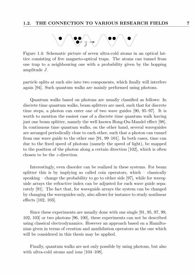
Figure 1.4: Schematic picture of seven ultra-cold atoms in an optical lat-tice consisting of five magneto-optical traps. The atoms can tunnel fromone trap to a neighbouring one with a probability given by the hoppingamplitude J .
particle splits at each site into two components, which finally will interfereagain [94]. Such quantum walks are mainly performed using photons.
Quantum walks based on photons are usually classified as follows: Indiscrete time quantum walks, beam splitters are used, such that for discretetime steps, a photon can enter one of two wave guides [90, 95–97]. It isworth to mention the easiest case of a discrete time quantum walk havingjust one beam splitter, namely the well known Hong-Ou-Mandel effect [98].In continuous time quantum walks, on the other hand, several waveguidesare arranged periodically close to each other, such that a photon can tunnelfrom one wave guide to the other one [91, 99–101]. In both cases, time candue to the fixed speed of photons (namely the speed of light), be mappedto the position of the photon along a certain direction [102], which is oftenchosen to be the z-direction.
Interestingly, even disorder can be realized in these systems. For beamsplitter this is by implying so called coin operators, which – classicallyspeaking – change the probability to go to either side [97], while for waveg-uide arrays the refractive index can be adjusted for each wave guide sepa-rately [91]. The fact that, for waveguide arrays the system can be changedby changing the waveguides only, also allows for instance to study nonlineareffects [102, 103].
Since these experiments are usually done with one single [91, 95, 97, 99,102, 103] or two photons [96, 100], these experiments can not be describedusing classical electrodynamics. However an approach based on a Hamilto-nian given in terms of creation and annihilation operators as the one whichwill be considered in this thesis may be applied.
Finally, quantum walks are not only possible by using photons, but alsowith ultra-cold atoms and ions [104–108].

8 INTRODUCTION
1.2.2 Ultra-cold Atoms in Optical Lattices
These systems consist of several atoms, which are at very low tem-peratures (usually a few nK) trapped in a periodic potential built up byinterfering laser beams, which are adjusted such that they form standingwaves [109] and are generally described by Hubbard models [110]. An op-tical lattice consisting of five magneto-optical traps, which are often alsodenoted as sites, and seven particles is schematically shown in Fig. 1.4.
An advantage of these systems is their vast controllability [111]. Byusing Feshbach resonances [112–115] for instance, the scattering length,which in turn determines the interaction strength, can be adjusted andtuned within a wide range [116, 117].
Additionally, by increasing the intensities of the used laser beams, thetunneling probability, i.e. the probability for an atom to tunnel from onewell of the optical lattice to another one, can be decreased, resulting in arelative increase of the interactions compared to the kinetic energy, whichis often denoted as hopping amplitude. If the tunneling probability is in-creased so far that the hopping amplitude is much smaller than the interac-tion strength, the energy is dominated by the latter and tunneling from onewell to an other is energetically suppressed or even forbidden. This regimeis called the Mott insulating phase [118, 119] and for ultra-cold atoms it isaccessible by the prescribed procedure. In fact, when increasing the laserintensity, bosonic ultra-cold atoms undergo a quantum phase transitionfrom a superfluid to a Mott insulating phase [120, 121].
For Fermions the Mott insulating phase also appears when the hoppingamplitude is not negligible but much smaller than the interaction strengthfor half filling and a phase transition from Mott insulating to superconduct-ing can be achieved by hole doping, i.e. by removing particles [122–124].For fermions, the Mott insulating ground state is also predicted to be an-tiferromagnetic [123].
The Mott insulating phase also allows a simple scheme for loading anoptical lattice with atoms [125–127]. In the same way, it can be used, forfixing the atoms after time evolution and determine the number of atomsin each well by high resolution imaging techniques [128, 129].
Finally, the energy of each well of the periodic potential can also beadjusted individually, thus giving the possibility to create optical disorder[130] and, despite the fact that atoms have no electrical charge (thereforea magnetic field does not have any effect on their motion) time reversalinvariance can be broken by artificial [131–134] and synthetic gauge fields[135].

1.2. THE CONNECTION TO VARIOUS RESEARCH FIELDS 9
These properties and especially the high controllability of the systemssuggest that ultra-cold atoms can be used as simulators for condensed mat-ter systems [111, 125] like for example graphene [136]. Since recently alsospin-orbit interaction have been realized with ultra-cold atoms [137–139],one could also think of simulating spintronics in optical lattices.
1.2.3 Spintronics
Spintronics is essentially the investigation of spin related effects, mainlysolid state systems, and aims towards a spin-based, rather than the con-ventionally charge-based, information transport [140–142]. The punchlinesthere, are e.g. the generation of spin polarization, injection of spin polar-ized currents as well as possibilities to manipulate and measure them. Veryoften hetero-structures composed of ferromagnetic materials and semicon-ductors or ferromagnetic and insulating materials are used. In these sys-tems, the ferromagnets serve as injectors or detectors of spin polarization.Very prominent effects in such hetero-structures are giant magnetoresis-tance (GMR) [143, 144] and tunneling magnetoresistance (TMR) [145].For both, GMR and TMR, the (electrical) resistance is much larger if themagnetizations of the two ferromagnetic layers have opposite directionsthan if they are parallel. The difference in the setup between them isthat for GMR a semiconductor is placed between two ferromagnets, whilefor TMR a so called magnetic tunnel junction is used, where an insulator(=tunneling barrier) is sandwiched by two ferromagnets. These two effectsalso made successfully their way to industrial applications and have beenestablished in read heads in hard disk drives.
Another effect, which seems to be on its way to industrial applicationsin so called racetrack memory [142] are spin transfer torque effects [146].In these effects, spin-polarized particles crossing a domain wall in a ferro-magnetic material transfers its magnetic moment to the substrate and thusmoves the domain wall.
Relativistic effects like Bychkov-Rashba [147] and Dresselhaus spin-orbit interactions [148] are also important in spintronics. For instance,they are the key elements of spin-hall [149, 150], quantum spin hall [151–154] and spin-based transistors [155]. While spin hall and quantum spinhall effect are both based on the fact that due to intrinsic spin-orbit in-teraction particles with spin up and spin down, respectively, moving inthe same direction are dragged to opposite directions perpendicular to theoverall direction of the current, in the spin field effect transistor [155] the

10 INTRODUCTION
spin orbit interaction strength is determined by an external gate voltage.The spin-orbit coupling then leads to spin-precession of the crossing parti-cle. The source and drain are magnetized, such that the electrons enteringare also spin-polarized and can enter the drain only if the spin-precessionis such that their spins are parallel to the magnetization in the drain.
So far, spintronics mainly focuses on single-particle effects [140–142,156], for which using a Fock space approach of indistinguishable particles isnot quite reasonable. However, for studying many-body effects in spintron-ics devices, the techniques developed in this thesis might be of particularhelp.
1.2.4 Many-Body effects in condensed matter physics
More generally, it is important to study many-body effects in condensedmatter systems. Well known amongst these are for instance the Coulombblockade [157–163], inelastic and elastic co-tunneling [164–168] and theKondo effect [168–170]. The Coulomb blockade arises due to the Coulombrepulsion of the electrons in a quantum dot coupled to leads via tunneljunctions. This repulsion implies a large energy cost in order to add afurther electron which in turn results in peaks of the current-voltage char-acteristic only for specific voltages corresponding to the energy needed inorder to add a electron to the quantum dot.
In quantum dots, cotunneling, where two electrons – one into the quan-tum dot and one out of the quantum dot – tunnel at the same time, andthe Kondo effect are corrections to the Coulomb blockade at low temper-atures. The Kondo effect originally refers to a minimum of the resistanceas a function of temperature in a metal [170] due to scattering off mag-netic impurities, where the impurity and the electron exchange their spin.Nowadays, the Kondo effect is mainly studied in quantum dots and carbonnanotubes [168, 171–188] and became a test case for many-body theoriesin condensed matter physics [189–196].
Due to their similarities, quantum dots are also regarded as artificial(two dimensional) atoms [177, 197, 198] and even the formation of artificialmolecules [199–201] is possible using quantum dots.

1.3. OUTLINE OF THIS THESIS 11
1.2.5 Chemical Physics
Real Atoms and Molecules, on the other hand, are the central objects inchemistry. In fact, the chemical physics community has made extensive useof semiclassical methods and played an important role in their development[70, 202–209].
Starting with Ref. [209] Miller and coworkers started the study of molec-ular collisions, which give rise to electronic transitions within the moleculesand succeeded to describe resonance effects [210]. There, the electronic de-grees of freedom have been treated semiclassically, while the nuclear motionwas incorporated classically [209]. After that, in order to be able to de-rive electronic and nuclear motion on the same footing, they turned toderiving a classical theory of these collisions [85, 211–213]. These classicalapproaches are basically determined by a mapping of angular momenta,including spin, to classical action angle varibles [202, 214].
Motivated by this process, Miller and White tackled the problem of de-riving a classical Hamiltonian for a second quantized fermionic Hamilonianalready in 1986 [86]. By using similar techniques they managed to derivea Schwinger representation of the angular momentum [215]. Later on, ithas been used heuristically in a semiclassical initial value representationincluding Langer substitutions [216].
The thus developed techniques have also been applied to electronictransport through a single quantum dot [217], two coupled quantum dots[218] and molecular junctions [219].
The problem with the Meyer-Miller-Stock-Thoss approach developedin [85, 86, 215, 216] is, however, that the Fock states, i.e. those stateswith well defined occupations of the single-particle states, are fixed pointsof the classical motion [220]. Moreover, it is based on heuristic mappingapproaches, instead of a rigorous derivation by means of a path integral,where the classical Hamiltonian appears naturally. Finally, it does notyield any insight, what the effective Planck constant heff , i.e. the smallparameter in a stationary phase analysis of the path integral, actually is.
1.3 Outline of this thesis
During this thesis, an answer to this last question, what the effectivePlanck constant is, will be also given. This will be accomplished by firstderiving an exact path integral both for Bosons and Fermions based on

12 INTRODUCTION
complex variables, which will also determine the classical limit of the secondquantized theory.
Before that, however, a brief introduction to the basic concepts usedduring this thesis will be given in the first part. This introduction containsa short review of the derivation of the path integral and the van-Vleck-Gutzwiller propagator in configuration space in Chapter 2, the basic con-cepts of second quantization as well as important states in Fock space andtheir properties in Chapter 3 for both, Bosons and Fermions.
The second part, finally, is dedicated to the construction of path in-tegrals and semiclassical approximations for the propagator in Fock spacebased on complex variables for Bosons in Chapter 4 as well as for Fermionsin Chapter 5. For the bosonic proapgator, it is also shown that the semi-classical approximation fulfills the semi-group property.
The thus derived bosonic propagator is applied in Part III to bosonicmany-body systems, starting with non-interacting systems like quantumwalks in photonic wave guide arrays in Chapter 6, and then turning todescribing coherent backscattering in Fock space for interacting particlesin Chapter 7, many-body transport of interacting Bosons in Chapter 8 andfinally to the fidelity decay for interacting ultra-cold atoms in Chapter 9.
Similarly, in the fourth part of this thesis, fermionic many-body interfer-ence effects are considered by applying the approach derived in Chapter 5.These interference effects are enhanced and vanishing transition probabili-ties between Fock states, which are investigated in Chapter 10, as well as amany-body spin echo resulting from an intermediate manipulation of spinsin Chapter 11 and a related quantity, which is here denoted as spin fidelityin Chapter 12.
Finally, concluding remarks as well as future perspectives are given inChapter 13.

Part I
Basic concepts
13


CHAPTER 2Semiclassics for
Single-Particle Systems
2.1 The Path Integral Representation of thePropagator
2.1.1 The quantum mechanical propagator
Semiclassics as it is understood through out this thesis, is based on astationary phase approximation to the quantum mechanical propagator (ortime evolution operator), which is defined as the operator which connectsthe state |ψ(ti)〉 at initial time ti with the one at final time tf , |ψ(tf )〉 by[221]
|ψ(tf )〉 = K(tf , ti) |ψ(ti)〉 . (2.1)
Since in quantum mechanics |ψ(t)〉 satisfies the time dependent Schrodingerequation
ih∂
∂t|ψ(t)〉 = H(t) |ψ(t)〉 ,
the propagator is the solution to the operator differential equation [13, 62]
ih∂
∂tK(t, ti) = H(t)K(t, ti), (2.2)
with initial condition
K(tf = ti, ti) = 1, (2.3)
15

16 SEMICLASSICS FOR SINGLE-PARTICLE SYSTEMS
where H(t) is the (time-dependent) quantum mechanical Hamilton oper-ator (or in short, quantum Hamiltonian), 1 is the unity operator, t is thetime, i is the imaginary unit and h is Planck’s constant.
Formally, the solution of eqns. (2.2,2.3) can be written as [62, 221]
K(tf , ti) = T exp
− i
h
tf∫ti
dtH(t)
, (2.4)
where T is the time ordering operator, which sorts the factors of the productright to it such that their time arguments decrease from left to right, e.g. fora product of two operators A1(t) and A2(t) [13, 62],
T A1(t1)A2(t2) =
A1(t1)A2(t2) if t1 ≥ t2,A2(t2)A1(t1) if t2 > t1.
More generally, for n operators A1(t), . . . , An(t),
Tn∏j=1
Aj(tj) =∑σ∈Sn
n−1∏j=1
Θ(tσ(j) − tσ(j+1)
) n∏j=1
Aσ(j)(tσ(j)), (2.5)
where the product∏j is defined such that j increases from left to write,
and Sn is the symmetric group of n, i.e. the group of all n-permutations,and
Θ(x) =
1 if x ≥ 0,
0 if x < 0.
is the Heaviside step function. A product of the form (2.5) is often alsodenoted as time-ordered product.
The combination T exp (. . .), as it appears in (2.4) and is usually calledtime-ordered exponential, should be evaluated by first expanding the ex-ponential using its Taylor series and after that applying the time orderingoperator to each summand individually. Note that, although[
H(t), H(t)]−
= 0,
the Hamiltonian at time t does in general not commute with the Hamilto-nian at time t′, [
H(t), H(t′)]−6= 0.

2.1. THE PATH INTEGRAL FOR THE PROPAGATOR 17
Here[A, B
]−
denotes the commutator of the operators A and B.
In order to further evaluate the propagator, one has to choose a cer-tain basis. In principle, one could choose any basis, however since thispart is meant for illustration of the basic methods used later on only theconfiguration space basis, given by the position eigenstates |r〉 is used here.
Inserting a unit operator in terms of position eigenstates [221, 222],
1 =
∫dDr |r〉 〈r| , (2.6)
where D is the spatial dimensionality of the systemm, in (2.1) and project-ing it to the position eigenstate |r〉 yields for the evolved wavefunction inconfiguration space [223]
ψ (r, tf ) =
∫dDr′K
(r, tf ; r′, ti
)ψ(r′, ti
),
where ψ(r, t) = 〈r|ψ(t)〉 and
K(r, tf ; r′, ti
)=⟨r∣∣∣ K (tf , ti)
∣∣∣ r′⟩ (2.7)
is the propagator in configuration space representation. The modulussquare of this complex quantity then yields the probability that if a particleis at time ti at position r′, it is found at time tf at position r. Therefore,by choosing the initial state to be a Dirac delta in configuration space,ψ(r′, ti) = δ (r′ − r), due to the normalization of the wave function,∫
dDr′∣∣K (r′, tf ; r, ti
)∣∣2 = 1.
Moreover, the initial condition of the propagator (2.3) reads in configura-tion space
K(r′, t; r, t
)= δ
(r′ − r
).
Finally, the time evolution operator has to be unitary and satisfy [13]
K(tf , t)K(t, ti) = K(tf , ti)
for any time t, i.e. propagating a state twice in time has to result in the samewave function as propagating it once over the whole duration. Moreover,it has to be unitary [13]. Thus, the propagator in configuration space has

18 SEMICLASSICS FOR SINGLE-PARTICLE SYSTEMS
to satisfy the semi-group properties∫dDr′′K
(r′, tf ; r′′, t
)K(r′′, t; r, ti
)=K
(r′, tf ; r, ti
), (2.8a)∫
dDr′′K∗(r′′, tf ; r′, t
)K(r′′, t; r, ti
)=K
(r′, tf ; r, tf
), (2.8b)
for any arbitrary time t.
2.1.2 The Path integral
Despite all these nice properties, one still has to evaluate the time or-dered product, in order to find the propagator in configuration space rep-resentation, a very difficult problem without general solution. However,Feynman found a way out of this problem by his famous path integralapproach [9]. Here we follow mainly Refs. [12, 13].
First, Trotter’s formula [224] is used, in order to split the time orderedexponential into an (infinite) product of exponentials with (infinitesimaly)small time steps [12, 13],
T exp
i
h
tf∫ti
dtH(t)
= limM→∞
M∏m=1
exp
[− iτ
hH(tf −mτ)
], (2.9)
where τ = (tf − ti) /M . Recall that the product is defined such that thevalue of m increases from left to right.
Using (2.9) in (2.7), inserting a unit operator in position representation(2.6) between ever two exponentials and finally a unit operator in momen-tum representation [222],
1 =
∫dDp |p〉 〈p| ,
left to every exponential, yields the path integral representation of thepropagator in position space,
K(r, tf ; r′, ti
)= lim
M→∞
∫dDp0
∫dDr1
∫dDp1 . . .
∫dDrM
∫dDpM
M∏m=0
〈rm+1 |pm〉⟨
pm
∣∣∣∣ exp
[− iτ
hH (ti +mτ)
] ∣∣∣∣ rm⟩,

2.1. THE PATH INTEGRAL FOR THE PROPAGATOR 19
where r0 = r′ and rM+1 = r. The matrix elements can then be evaluatedby making use of the fact that the quantum Hamiltonian has the form
H =1
2µp2 + V (r),
where µ is the mass of the particle, V (r) the potential and p and r themomentum and position operator, respectively. Using the Baker-Campbell-Hausdorff formula [13], in the limit M →∞, each exponential can be splitinto two exponentials, where the first one consists of the momentum andthe second one depends on the position operator, only. Note that this doesnot apply in the presence of magnetic field, however one can show that thefinal form of the path integral is the same up to replacing the momentump by p− q
cA(r) with q, c and A being the charge of the particle, the speedof light and the vector potential, respectively [12]. Then, one can let actevery momentum operator to the left and every position operator to theright, finally yielding [12, 13]
K(r, tf ; r′, ti
)=
limM→∞
∫dDp0
(2πh)D
∫dDr1
∫dDp1
(2πh)D. . .
∫dDrM
∫dDpM(2πh)D
exp
i
h
M∑m=0
[pm · (rm+1 − rm)− τH (pm, rm; ti +mτ)]
,
(2.10)
with the classical Hamiltonian resulting from the quantum one by replac-ing the momenum and position operator by real numbers, which are themomentum and position, respectively,
H (p, r) =p2
2µ+ V (r) . (2.11)
Eq. (2.10) is often written in the short-hand notation [13]
K(r, tf ; r′, ti
)=
r∫r′
D [p(t), r(t)] exp
(i
hR [p(t), r(t)]
),
where the limits of the integral indicate that the initial and final positionsare fixed to r′ and r, respectively and
R [p(t), r(t)] =
tf∫ti
dt [p · r−H (p(t), r(t); t)]

20 SEMICLASSICS FOR SINGLE-PARTICLE SYSTEMS
is the action of the path (p(t), r(t)).
The name “path integral” comes from the fact that the integral∫D [p(t), r(t)] . . .
runs over all paths in phase space. These paths, which are schematicallydepicted in Fig. 2.1(a), are neither restricted to the (classically) allowedregions nor do they need to be smooth.
Finally, making use of the form (2.11) of the classical Hamiltonian theintegrals over the intermediate momenta can be carried out [12, 13],
K(r, tf ; r′, ti
)=
limM→∞
∫dDr1 . . .
∫dDrM
exp
iτh
M∑m=0
[µ2τ (rm+1 − rm)2 − τV (rm)
](2πihτ/µ)
D(M+1)2
,
(2.12)
which finally connects the propagator with the Lagrange function of thesystem by [13, 94]
K(r, tf ; r′, ti
)=
r∫r′
D [r(t)] exp
(i
hR [r(t), r(t)]
), (2.13)
with the action of the path (r(t), r(t))
R [r(t), r(t)] =
tf∫ti
dtL (r(t), r(t); t) =
tf∫ti
dt(µ
2r2(t)− V (r(t))
).
It is important to notice that the path integral runs over paths that arenot necessarily restricted to the classically allowed region.
The huge advantage of the path integral representation is that oneclearly sees the origin of interference: There are essentially an infinite num-ber of possible paths a particle can take. However, during its evolution itwill pick up a phase, which is given by the action of this path, and thereforeevery path yields a different phase. Finally, all paths add up and thereforeinterference occurs.

2.2. THE SEMICLASSICAL APPROXIMATION 21
(a) Possible paths summedover in the path integral
(b) Classical paths among thequantum ones shown in (a) se-lected by the stationarity con-dition
Figure 2.1: Selection of classical paths due to the stationary phase con-dition. The shaded areas mark classically forbidden regions. While thequantum paths can be non-smooth and cross these regions the classicalones can not
2.2 The Semiclassical Approximation
The path integral (2.12) is also the starting point for the semiclassicalapproximation to the propagator. It is based on the observation that inmany relevant cases, the actions are much largher than h. Then the inte-grals in (2.12) can be evaluated using the stationary phase approximation[11].
2.2.1 Stationary phase approximation
The stationary phase approximation is a method to evaluate integralsof the form
I =
∞∫−∞
dxg(x) exp [iλf(x)] ,
where λ 1 is a large parameter and g(x) a smooth function. As illustratedfor the case of the integral representation for the Bessel function in Fig. 2.2,the integrand oscillates very fast as a function of x except for those valuesof x close to the stationary points x1, . . . , xn of f , for which
∂
∂xf(x)
∣∣∣∣x=xj
= 0. (2.14)
Therefore, one first splits the integral into n integrals, where the j-th in-tegral runs over an interval containing the j-th stationary point and the

22 SEMICLASSICS FOR SINGLE-PARTICLE SYSTEMS
-1
-0.5
0
0.5
1
0 0.2 0.4 0.6 0.8 1
τ
(a) Comparison between the exact (red) in-tegrand and the one in the stationary phaseapproximation (blue) for the integral rep-resentation of the fifth Bessel function atx = 65.
-60
-40
-20
0
20
0 0.2 0.4 0.6 0.8 1
τ
(b) Argument of the integrand for the inte-gral representation of the fifth Bessel func-tion at x = 65.
Figure 2.2: The integrand of the integral-representation of the n-th Besselfunction, Jn(x) =
∫ π0 τ cos [nτπ − x sin (τπ)], strongly oscillates except in
the region around x ≈ 0.47549 ((a), where the argument of the cosine isstationary (b). Therefore, the main contribution to the integral stems fromthis region.
exponential is expanded up to second order around the stationary point.Dropping the higher order contributions of f(x) yields an error of the orderof 1/λ [12]. Since the main contributions to I stem from regions close to thestationary points – more precisely from the interval [x− 1/
√λ, x+ 1/
√λ]
[12] – each integral can be extended to the whole real axes,
I ≈n∑j=1
∞∫−∞
dxg(x+ xj) exp
[i
h
(f(xj) +
1
2f ′′(xj)x
2
)],
with f ′′ denoting the second derivative of f . Fig. 2.2(a) shows for the caseof the Bessel function how this approximation indeed resembles the exactintegral, within the region where it varies slowly, very well. Expandingg(x− xj) around zero then allows to compute the integrals term by term,where the contributions from the x-dependent terms of g again lead tocontributions of the order 1/λ, whereas the leading order contribution isof the order of 1/
√λ [12]. Thus, finally I is within the stationary phase

2.2. THE SEMICLASSICAL APPROXIMATION 23
approximation given by [12, 13]
I ≈n∑j=1
g(xj)
√2πi
λf ′′(xj)exp [iλf(xj)]
=
n∑j=1
g(xj)
√2π
λ |f ′′(xj)|exp
[iλf(xj) + i
π
4sign
(f ′′(xj)
)].
(2.15)
with an error of the order 1/λ.For higher dimensional system, the same steps can be performed and
yields for scalar functions g(x) and f(x) [14]∫dDxg(x) exp [iλf(x)] ≈
n∑j=1
g(xj)
√(2πi)D
λD det ∂2f∂x2 (xj)
exp [iλf(xj)]
=
n∑j=1
g(xj)
√√√√ (2π)D
λD∣∣∣det ∂
2f∂x2 (xj)
∣∣∣ exp[iλf(xj) + iβ (xj)
π
4
]
=n∑j=1
g(xj)
√√√√ (2πi)D
λD∣∣∣det ∂
2f∂x2 (xj)
∣∣∣ exp[iλf(xj)− iν (xj)
π
2
],
(2.16)
whereβ (x) = D − 2ν (x) ,
and ν(xj) is the number of negative eigenvalues of the matrix of secondderivatives of f . Thus, β(x) is the difference in the number of positive andnegative eigenvalues of ∂2f/∂x2.
Note that since in semiclassics this approximation is used frequently, itis also called the semiclassical approximation. Moreover, since the station-ary phase approximation requires a large parameter in the phase, which isin semiclassics usually 1/h, the inverse of the large parameter, i.e. in thissection 1/λ is called the effective Planck’s constant heff
2.2.2 The van-Vleck-Gutzwiller Propagator
It was Martin C. Gutzwiller [11], who first applied the stationary phaseapproximation (2.16) to Feynman’s path integral (2.12). In terms of func-tional derivatives the stationarity condition (2.14) for the propagator reads

24 SEMICLASSICS FOR SINGLE-PARTICLE SYSTEMS
δ
δr(t)R [r(t), r(t)] =
d
dt
∂L∂r(t)
− ∂L∂r(t)
= 0, (2.17)
still with fixed boundary conditions r(ti) = r′ and r(tf ) = r. Eq. (2.17)is exactly Hamilton’s principle of the least action and leads to the Euler-Lagrange equations. Thus, the stationary phase approximation selects fromall paths only the classical trajectories starting at intitial position r′ andending at the final one r (see Fig. 2.1 for a schematic example). Note that,in general, there might be several classical trajectories joining the two endpoints and thus following Eqns. (2.15,2.16) the semiclassical propagatorwill be a sum over classical trajectories, rather than just one term.
The semiclassical propagator in configuration space has thus the form
K(sc)(r, tf ; r′, ti
)=∑
γ:r′→r
Aγ(r, tf ; r′, ti
)exp
[i
hRγ(r, tf ; r′, ti
)+ iνγ
(r, tf ; r′, ti
) π2
],
where the sum runs over all trajectories of the corresponding classical sys-tem joining the inital and final points r′ and r,
Aγ(r, tf ; r′, ti
)= lim
M→∞
( µ
2πihτ
)D2
∣∣∣∣detτ
µδ2RM
∣∣∣∣− 12
(2.18)
is the semiclassical amplitude and νγ (r, tf ; r′, ti) is the number of negativeeigenvalues of
δ2RM =∂2
∂ (r1, . . . , rM )2
M∑m=0
[ µ2τ
(rm+1 − rm)2 − τV (rm)],
which is the matrix of the second derivatives of the (discrete) action. Both,the semiclassical amplitude Aγ and the phase νγ have to be evaluated inthe limit M →∞ and along the classical trajectory γ.
Connecting Aγ and νγ with classical quantities is the actual achieve-ment of Gutzwiller’s work [11]. He recognized that Morse’s theory [225, 226]identifies νγ with the number of conjugate points of the trajectory γ.Therefore, νγ is also called Morse index. A conjugate, or sometimes alsocalled focal point, of a trajectory is the position, at which the deriva-tive ∂r(t)/∂p(ti) vanishes, i.e. all trajectories, starting at the same ini-tial position r′, but with slightly different momenta within the interval[p(ti)− δp/2,p(ti) + δp/2] will cross each other at time t in the conjugatepoint r(t) [6] (see Fig. 2.3).

2.2. THE SEMICLASSICAL APPROXIMATION 25
Conjugate point
r′
r
Figure 2.3: Points in configuration space, at which trajectories with slightlydifferent initial momenta but same initial position coincide are called con-jugate points.
The connection of det δ2RM with a classical quantity can be foundfollowing e.g. [14]. First, one notices that the matrix δ2RM is block-tridiagonal,
δ2RM =µ
τ
d1 −ID 0 . . . 0−ID d2 −ID 0 . . . 0
. . .
0 . . . 0 −ID dM−1 −ID0 . . . 0 −ID dM
,
where dj = 2ID − τ2
µ∂V∂r2 (rj) and ID is the D × D unit matrix. Since
the off-diagonal entries are unit matrices and therefore commute with thediagonal ones, one can formally expand the determinant GM = det τµδ
2RMalong the last row, which yields the recursion relation
GM = det (dM )GM−1 −GM−2,
with the initial conditions G1 = det d1 and G0 = 1.On the other hand, from the stationarity condition for rM−1, one finds
rM = 2rM−1 −τ2
µ
∂V
∂r(rM−1)− rM−2,
which after taking the derivative with repsect to r1 and taking the deter-minant turns into
det∂rM∂r1
= det
[(2ID −
τ2
µ
∂2V
∂r2(rM−1)
)∂rM−1
∂r1
]− det
∂rM−2
∂r1
= det (dM−1) det∂rM−1
∂r1− det
∂rM−2
∂r1.

26 SEMICLASSICS FOR SINGLE-PARTICLE SYSTEMS
The initial conditions for this determinant are given by
det∂r1
∂r1= 1
det∂r2
∂r1= det d1.
Therefore GM can be identified to be
GM = det∂rM+1
∂r1= det
µ
τ
∂rM+1
∂p0,
where in last equality, r1 = r0 + τµp0, with p0 being the initial momentum,
has been used. Thus, using p0 = −∂Rγ(r,tf ;r′,ti)∂r′ , (2.18) finally becomes
Aγ(r, tf ; r′, ti
)=
1
(2πih)D2
∣∣∣∣det∂2Rγ (r, tf ; r′, ti)
∂r∂r′
∣∣∣∣12
and therefore the semiclassical propagator in configuration space is finallygiven by the van-Vleck-Gutzwiller propagator
K(sc)(r, tf ; r′, ti
)=∑γ:r′→r
1
(2πih)D2
√∣∣∣∣det∂2Rγ∂r∂r′
∣∣∣∣ exp
(i
hRγ + i
π
2νγ
).
(2.19)Previous to Gutzwiller, van-Vleck already derived (2.19) from statisticalarguments [7], however missed the phase given by the Morse index. There-fore, in order to get the correct phases, the semiclassical propagator shouldalways be computed using the stationary phase approximation.
Moreover, for small propagation times, in (2.19) only one classical tra-jectory contributes, and thus the van-Vleck-Gutzwiller propagator turnsinto the short time propagator found by Pauli [8]. This equality showsthat for times smaller than a certain time scale, called Ehrenfest time tE ,the quantum evolution follows the classical one.
Finally, it should be noted that the stationary phase approximationbecomes exact if g(x) = const. and f(x) is a quadratic polynomial. There-fore, if the quantum Hamiltonian is quadratic in p and q, like for the freeparticle or the harmonic oscillator, the semiclassical van-Vleck-Gutzwillerpropagator (2.19) is exact.

2.3. SEMICLASSICAL PERTURBATION THEORY 27
2.3 Semiclassical Perturbation Theory
One important and frequently used tool in semiclassics is the semiclas-sical perturbation theory. In conventional semiclassics it is mainly used inorder to include a weak magnetic field.
Although, it is widely used, there does not seem to be any reference forthe derivation of the semiclassical perturbation theory on the level of thepropagator, so it will be presented here.
Suppose, the quantum Hamiltonian can be decomposed into a non-perturbed one, for which for simplicity here momentum and position oper-ators are assumed to be separated, plus some small perturbation,
H = H0 + εV1 =p2
2µ+ V0 (r) + εV1 (p, r) ,
where ε is a measure of the strength of the perturbation.
When pluggin in this hamiltonian into the discrete path integral (2.10)and expanding the exponential in powers of ε, one finds
K(r, tf ; r′, ti
)=
limM→∞
∫dDp0
(2πh)D
∫dDr1
∫dDp1
(2πh)D. . .
∫dDrM
∫dDpM(2πh)D
exp
i
h
M∑m=0
[pm · (rm+1 − rm)− τH0 (pm, rm; ti +mτ)]
×∞∑k=0
(−iτε)k
hkk!
[M∑m=0
V1 (pm, rm)
]k.
(2.20)
Note that this formula also represents an expansion in terms of Feynmandiagrams, where the k-th term in the sum yields those diagrams where thesystem is evolved under the unperturbed Hamiltonian k+1 times with onescattering event due to the perturbation occurs between each evolution.
On the other hand, the semiclassical perturbation theory is achievedby evaluating the integrals in (2.20) in a stationary phase approximation.Since the stationary points are determined by the exponent only, the per-turbation has no effect on the classical trajectory, i.e. the sum will still beover the unperturbed trajectories.
After taking the limit M → ∞, one obtains the van-Vleck-Gutzwiller

28 SEMICLASSICS FOR SINGLE-PARTICLE SYSTEMS
propagator in semiclassical perturbation theory,
K(sc)(r, tf ; r′, ti
)=
∑γ0:r′→r
1
(2πih)D2
√∣∣∣∣det∂2Rγ0
∂r∂r′
∣∣∣∣exp
(i
hRγ0 + i
π
2νγ0
)
×∞∑k=0
1
k!
−iε
h
tf∫ti
dtV1 (µrγ0(t), rγ0(t))
k
.
Note that for a classical trajectory the relation p = µr holds, such that theperturbation is evaluated at the classical momentum and position and isfinally integrated over time.
Finally, the expansion in powers of ε can be undone, such that thesemiclassical perturbation theory is finally given by
K(sc)(r, tf ; r′, ti
)=
∑γ0:r′→r
1
(2πih)D2
√∣∣∣∣det∂2Rγ0
∂r∂r′
∣∣∣∣ exp
(i
hRγ0 + i
π
2νγ0
)
× exp
− iε
h
tf∫ti
dtV1 (pγ0(t), rγ0 (t))
,(2.21)
where the subscript 0 at the trajectory γ0 indicates that it is the trajectoryof the unperturbed classical system. Moreover, Rγ0 is the action of theunperturbed trajectory for ε = 0.
Within the semiclassical perturbation theory the classical trajectoriesare kept unchanged, while each term of the propagator is multiplied byan additional phase, which is given by the perturbation evaluated alongthe classical trajectory. Note that classically the momentum p and thetime derivative of the position r are related by p = µr and therefore theperturbation is evaluated at the momentum and position of the classicaltrajectory.
Now consider for a moment the derivative of the action of an exact clas-sical trajectory of the perturbed system. This derivative can be computed
2.3. SEMICLASSICAL PERTURBATION THEORY 29
as
∂
∂εRγε =
∂
∂ε
tf∫ti
dt [pγε · rγε −Hε (pγε , rγε)] =
tf∫ti
dt
∂pγε∂ε· rγε + pγε ·
∂rγε∂ε− ∂Hε
∂rγε
∂rγε∂ε− ∂Hε
∂pγε
∂pγε∂ε− V1 (pγε , rγε)
.
Using Hamilton’s equations of motion, the two terms containing the deriva-tive of the momentum with respect to ε cancel, such that after a partialintegration of the term p · ∂r/∂ε, one gets
∂
∂εRγε =
[pγε ·
∂rγε∂ε
]tfti
−tf∫ti
dt
[pγε ·
∂rγε∂ε
+∂Hε
∂rγε
∂rγε∂ε
]−
tf∫ti
dtV1 (pγε , rγε)
=−tf∫ti
dtV1 (pγε , rγε) ,
where in the last step again Hamilton’s equations of motion have been usedas well as the fact that the intial and final positions are fixed and thereforeindependent of ε.
If the perturbation is small enough the trajectories are only slightlydeformed by the perturbation, such that there is a one-to-one correspondingbetween perturbed and unperturbed trajectories. Therefore, the phase in(2.21) is the expansion of the classical action up to linear order in ε, whilein the prefactor, only the constant term in the expansion in ε is kept.


CHAPTER 3From Single- to Many-Body
Physics: Secondquantization and many-body
states
3.1 Second Quantization and Fock states
In this section the basic concepts of second quantization will be reviewedvery briefly, while a more detailed description can be found e.g. in [227].
The basic idea of second quantization is to describe a system of manyidentical and indistinguishable particles by utilizing the solutions of thecorresponding single-particle system. This is possible by noticing thatthe many-body Hilbert space can only be constructed from single-particlestates.
It turns out to be useful to introduce the occupation number nl, whichis the number of particles, occupying the (normalized) single-particle statel. For Bosons, these numbers can be any integer from zero to infinity, whilefor Fermions – due to the Pauli principle – they are either 0 or 1. Hereit should be noted that the spatial single-particle state and the spin statetogether form the single-particle state, such that a spin up and spin downparticle in the same spatial (or orbital) single-particle state are regarded asparticles occupying two different single-particle states (see Fig. 3.2). With
31

32 SECOND QUANTIZATION AND MANY-BODY STATES
(a) |1, 0, 0, 0, 0〉 (b) |1, 2, 1, 4, 3〉 (c) |1, 0, 1, 1, 0, 0, 0, 0, 0, 1〉
Figure 3.1: Illustration of the definitions of Fock states for a quantum wellwith five bound states for (a) one spin-less particle, (b) eleven spin-lessparticles and (c) four spin-1/2 particles.
Figure 3.2: A spin-up and spin-down particle in the same spatial (or orbital)single-particle state are regarded as particles occupying two different single-particle states.
these occupation numbers, each many-body state with given symmetryunder exchange of particles (symmetric for Bosons and antisymmetric forFermions), can be represented by a Fock state (see also Fig. 3.1)
|n〉 = |n1, n2, . . .〉 .
Fock states are orthonormal,⟨n∣∣n′⟩ =
∏l
δnl,n′l
= δn,n′
and complete, ∑n
|n〉 〈n| = I.
The space spanned by these Fock states (including the so called vacuumstate |0〉 = |0, 0 . . .〉), is called Fock space.

3.1. SECOND QUANTIZATION AND FOCK STATES 33
(a) |1, 2, 1, 3, 3〉 (b) |1, 2, 1, 4, 3〉
a†4
a4
Figure 3.3: Applying the creation operator a†4 to the bosonic state in (a)results in the state shown in (b), while with the help of the annihilationoperator a4, one can go from left to right.
Since nl is the number of particles in state l, one can easily find thesubspace of fixed total number of particles N . This is the space spannedby all Fock states |n〉 which satisfy∑
l
nl = N.
Within the procedure of second quantization, one also defines creationand annihilation operators. Since their properties and actions on the Fockstates depends on whether the described particles are Bosons or Fermions,from now on these two cases are discussed separately.
3.1.1 Bosonic creation and annihilation operators
The bosonic creation and annihilation operators will be denoted by a†land al, respectively, throughout the entire thesis. The creation operator a†lincreases the number of particles in the single-particle state l by one (seeFig. 3.3),
a†l |n1, . . . , nl, . . .〉 =√nl + 1 |n1, . . . , nl + 1, . . .〉 .
Analoguously, the annihilation operator al is defined as the operatordecreasing the number of particles in the single-particle state l,
al |n1, . . . , nl, . . .〉 =√nl |n1, . . . , nl − 1, . . .〉 .

34 SECOND QUANTIZATION AND MANY-BODY STATES
This definition of the annihilation operators also implies that applyingal to a Fock states with nl = 0 yields zero,
al |n1, . . . , nl−1, 0, nl+1, . . .〉 = 0.
These definitions also require that the commutation relations for cre-ation and annihilation operators to read[
a†l , a†l′
]−
= 0 (3.1a)
[al, al′ ]− = 0 (3.1b)[al, a
†l′
]−
= δl,l′ , (3.1c)
where [A, B
]−
= AB − BA
is the commutator of the operators A and B.
It is important to notice that any Fock state |n〉 = |n1, n2, . . .〉 can be
derived by applying the creation operator a†1 n1 times, n2 times the creation
operator a†2, etc., to the vacuum,
|n1, n2, . . .〉 =1√
n1!n2! · · ·(a†1
)n1(a†2
)n2 · · · |0〉 .
From the definitions of the creation and annihilation operators, it is easyto see that a Fock state is an eigenstate to the number operator nl = a†l alwith eigenvalue nl,
nl |n1, . . . , nl, . . .〉 = nl |n1, . . . , nl, . . .〉 .
Since the eigenvalue of nl is the occupation number of the l-th single-particle eigenstate, nl is refered to as the l-th number operator. Moreover,this allows to define the total number operator
N =∑l
nl.

3.1. SECOND QUANTIZATION AND FOCK STATES 35
(a) |1, 0, 1, 1, 0, 0, 0, 0, 0, 0〉 (b) |1, 0, 1, 1, 0, 0, 0, 0, 0, 1〉
a†4
a4
Figure 3.4: Applying the creation operator c†5↓ to the fermionic state in (a)results in the state shown in (b), while with the help of the annihilationoperator a5↓, one can go from left to right.
In the following chapters, the shorthand notations
a† =(a†1, a
†2, . . .
)(3.2a)
a =
a1
a2...
(3.2b)
n =
n1
n2...
(3.2c)
will also be used.
3.1.2 Fermionic creation and annihilation operators
The fermionic creation and annihilation operators c†l and cl are definedsimilarly as the bosonic ones. However, one has to keep in mind that dueto the Pauli principle, a particle can not be created in a state, which isalready occupied, such that
c†l |n1, . . . , nl−1, 0, nl+1, . . .〉 = (−1)
l−1∑l′=1
nl′ |n1, . . . , nl−1, 1, nl+1, . . .〉 (3.3a)
c†l |n1, . . . , nl−1, 1, nl+1, . . .〉 = 0 (3.3b)

36 SECOND QUANTIZATION AND MANY-BODY STATES
as well as
cl |n1, . . . , nl−1, 0, nl+1, . . .〉 = 0, (3.4a)
cl |n1, . . . , nl−1, 1, nl+1, . . .〉 = (−1)
l−1∑l′=1
nl′ |n1, . . . , nl−1, 0, nl+1, . . .〉 , (3.4b)
where the additional signs in (3.3a) and (3.4b) account for the antisymme-try of Fermions under exchange of particles.
Accordingly, the fermionic creation and annihilation operators obey cer-tain anticommutation relations, rather than commutatoin relations. Theseare [
c†l , c†l′
]+
= 0,
[cl, cl′ ]+ = 0,[cl, c
†l′
]+
= δl,l′ ,
with the anticommutator of two operators A and B given by[A, B
]+
= AB + BA.
The connection between a fermionic Fock state and the vacuum statetherefore reads
|n1, n2, . . .〉 = · · ·(c†2
)n2(c†1
)n1 |0〉 , (3.5)
where now it is crucial to apply the creation operators in the correct order,since exchanging two creation operators gives an additional minus sign.This additional minus sign is also the reason, why there has to be anadditional sign in equations (3.3a) and (3.4b).
In the same way as for Bosons, a number operator can be defined forFermions too,
nl = c†l cl.
The number operator has eigenvalues 0 and 1, with the eigenvectorsbeeing the Fock states,
nl |n1, . . . , nl, . . .〉 = nl |n1, . . . , nl, . . .〉 ,

3.1. SECOND QUANTIZATION AND FOCK STATES 37
and allows to define the total number operator
N =∑l
nl.
For the fermionic operators the shorthand notations
c† =(c†1, c
†2, . . .
)c =
c1
c2...
n =
n1
n2...
will also be used in the following chapters.
3.1.3 Hamiltonian and observables in second quantization
The whole theory of second quantization would be worthless, if many-body Hamiltonians and observables could not be expressed in terms ofcreation and annihilation operators. Here, general observables will be con-sidered since the Hamiltonian is just a special kind of observable, namelythe energy of the system.
In many-body systems, operators are classified by the number of parti-cles they couple. A n-body operator in second quantization is an operatorof the form
On =∑
i1,...,in,j1,...,jn
Oi1,...,in,j1,...,jn a†i1· · · a†in aj1 · · · ajn , (3.6)
where in this section, a†j and aj denote either fermionic or bosonic creationand annihilation operators for the j-th single-particle states. Here, thetensor elements Oi1,...,in,j1,...,jn are given by
Oi1,...,in,j1,...,jn =⟨in
∣∣∣ · · ·⟨i1 ∣∣∣ O ∣∣∣ j1⟩ · · · ∣∣∣ jn⟩ . (3.7)
Eq. (3.6) can be interpreted as removing n particles – each one from thesingle-particle states j1, . . . , jn – and put it to i1, . . . , jn with an amplitudegiven by (3.7). Finally, one has to sum over all possible of such processes.

38 SECOND QUANTIZATION AND MANY-BODY STATES
An n-body observable is then a linear hermitian combination of suchn-body operators and in general an observable may be given by the linearcombination of n-body observables with different values of n, e.g. a veryimportant Hamiltonian especially in the theory of ultra-cold atoms, is theHamiltonian for a 1-dimensional Bose-Hubbard chain with nearest neighborhopping and two-body on-site interactions,
H =
L∑l=1
εla†l al −
L−1∑l=1
(κa†l al+1 + κ∗a†l+1al
)+U
2
L∑l=1
a†l a†l alal. (3.8)
This Hamiltonian models for instance atoms in a chain of L magneto-optical traps, where the energy of the l-th trap is εl, the particles tunnelfrom one trap to the adjacent one with probability κ and the two bodyinteraction stems from s-wave scattering among particles within the sametrap. In order to arive at the Hamiltonian (3.8), the chosen basis for thesingle-particle state are the Wannier functions of the individual traps.
One should also notice that for a non-interacting many-body system,the many-body Hamiltonian in the eigenbasis of the single-particle Hamil-tonian is given by
H =∑j
Ej a†j aj =
∑j
Ejnj .
Moreover, in second quantization, the total number of particles is no longeran extrinsic parameter, but an observable
N =∑j
nj ,
which is conserved for closed systems.
3.2 Bosonic Many-Body States
Due to the fact that bosonic operators for different single-particle statescommute it is enough to consider only single-state systems in this section.
3.2.1 Quadrature States
In this section, we follow to some extend the consideration of quadratureeigenstates given in section 3.3.3 of [228].

3.2. BOSONIC MANY-BODY STATES 39
The quadrature states are defined as the eigenstates of the quadratureoperator,
x (ϕ) |x〉ϕ = x(ϕ) |x〉ϕx (ϕ) = b
[a exp (iϕ) + a† exp (−iϕ)
],
where b and ϕ are for now arbitrary, but real parameters.This definition can also be used, in order to express the annihilation
and creation operators in terms of quadrature operators,
aj =exp (−iϕ)
2b
[x (ϕ) + ix
(ϕ− π
2
)](3.9a)
a†j =exp (iϕ)
2b
[x (ϕ)− ix
(ϕ− π
2
)]. (3.9b)
Moreover, it is straight forward to compute the commutation relation ofthe quadrature operators,[
x (ϕ) , x(ϕ′)]
= 2ib2 sin(ϕ− ϕ′
). (3.10)
Since the quadrature operators are obviously hermitian, the eigenvaluesx are real. For the sake of generality, a dependence of the eigenvalueon the quadrature phase ϕ has been included. However, by making useof the commutation relations (3.1) it can be shown that for an arbitraryquadrature phase ϕ, the quadrature operator is related to the one withϕ = 0 by
x (ϕ) = exp(−iϕa†a
)x (0) exp
(iϕa†a
).
which plugged into the eigenvalue equation for ϕ = 0 yields
x |x〉ϕ=0 = x (0)x |x〉ϕ=0 = exp(
iϕa†a)x (ϕ) exp
(−iϕa†a
)|x〉ϕ=0
and therefore
x (ϕ) exp(−iϕa†a
)|x〉ϕ=0 = x exp
(−iϕa†a
)|x〉ϕ=0 ,
which shows that the eigenvalue x (ϕ) = x does not depend on the quadra-ture phase, and the quadrature eigenstate for non-zero phase is connectedto the one with ϕ = 0 by
|x〉ϕ = exp(−iϕa†a
)|x〉ϕ=0 . (3.11)

40 SECOND QUANTIZATION AND MANY-BODY STATES
This observation allows to compute properties for non-zero quadraturephases easily out of the quadrature eigenstates for ϕ = 0.
In order to shorten the notation, from now on the quadrature operatorswith zero quadrature phase will be denoted by q, the corresponding eigen-states by |q〉, as well as their eigenvalues by q. Likewise, the quadratureoperators for ϕ = −π/2 will be denoted by p as well as their eigenstates by|p〉 and their eigenvalues by p.
The expansion of the quadrature eigenstates |q〉 in Fock states can befound by considering
q
b〈n | q〉 =
1
b〈n| q |q〉 =
√n+ 1 〈n+ 1 | q〉+
√n 〈n− 1 | q〉 .
The normlized solution to this recurrence relation is given by [229]
〈n | q〉 =exp
(− q2
4b2
)√
2nn!√
2πbHn
(q√2b
),
where Hn denotes the n-th Hermite polynomial.Using (3.11), one immediately sees that for arbitrary ϕ,
〈n |x〉ϕ =exp
(− x2
4b2− inϕ
)√
2nn!√
2πbHn
(x√2b
)(3.12)
In the semiclassical treatment of the propagator, we will have to eval-uate integrals involving the overlap between quadrature and Fock states,which are very hard to compute. If the occupation number n is large, how-ever, one may use the asymptotic form of this overlap, which is - for ϕ = 0- given by the WKB-approximation [6],
〈n | q〉 ≈√√√√ 2
π√
4b2(n+ 1
2
)− q2
cos[F (q, n) +
π
4
], (3.13)
where F (q, n) is the generating function for the canonical transformation
from (q, p) to (n, θ) with q = 2b√n+ 1
2 cos θ and p = 2b√n+ 1
2 sin θ and
is given by
F (q, n) =q
4b2
√4b2(n+
1
2
)− q2 −
(n+
1
2
)arccos
q
2b√n+ 1
2
.
3.2. BOSONIC MANY-BODY STATES 41
It is worth to notice that the generating function can also be written as anintegral along a classical path,
F (q, n) =1
b
q∫q0
dx
√n+
1
2− x2
4b2,
where q0 = 2b√n+ 1/2. As a generating function of a canonical transfor-
mation, the derivatives of F (q, n) satisfy
∂F (q, n)
∂q=
1
b
√n+
1
2− q2
4b2=|p|2b2
∂F (q, n)
∂n= − arccos
q
2b√n+ 1
2
= −θ
Note that, by this definition of θ, the phase is only defined between 0 andπ, and therefore |p| = p.
Having found the overlap (3.12) and using the properties of the Her-mite polynomials, one can also find the overlap between two quadratureeigenstates as well as the resolution of unity,
⟨x∣∣x′⟩
ϕ ϕ′=
exp
[i2xx′−(x2+x′2) cos(ϕ−ϕ′)
4b2 sin(ϕ−ϕ′)
]b√
2π (1− exp [2i (ϕ− ϕ′)])for ϕ 6= ϕ′, (3.14a)⟨
x∣∣x′⟩
ϕ ϕ= δ
(x− x′
), (3.14b)
∞∫−∞
dx |x〉ϕ 〈x|ϕ = 1, (3.14c)
and in particular for ϕ′ = ϕ− π/2,⟨x∣∣x′⟩
ϕ ϕ−π2
=1√
4b2πexp
(i
2b2xx′). (3.15)
Thus, for fixed ϕ, the quadrature eigenstates |x〉ϕ form a continuous, butcomplete and orthogonal basis of the Fock space.
In the following chapters,⟨x∣∣ a ∣∣x′⟩
ϕ−π2
ϕ=
1
4b2√π
(x′ + ix
)exp
(− i
2b2xx′), (3.16a)⟨
x∣∣∣ a† ∣∣∣x′⟩
ϕ−π2
ϕ=
1
4b2√π
(x′ − ix
)exp
(− i
2b2xx′), (3.16b)

42 SECOND QUANTIZATION AND MANY-BODY STATES
will also be used. Eq. (3.16) follows immediately from the representation ofthe creation and annihilation operators in terms of quadrature operators,Eq. (3.9).
Using the resolution of unity, Eq. (3.14c), as well as Eq. (3.16), it isstraight forward to compute,⟨
x∣∣ a ∣∣x′⟩
ϕ ϕ=
(1
2bx− b ∂
∂x
)δ(x− x′
)(3.17a)⟨
x∣∣∣ a† ∣∣∣x′⟩
ϕ ϕ=
(1
2bx− b ∂
∂x′
)δ(x− x′
)(3.17b)
3.2.2 Coherent States
Coherent states are defined as the eigenstates of the anihilation opera-tor,
a |φ〉 = φ |φ〉 .Since the annihilation operators are non-hermitian, the eigenvalues φ arein general complex. One can show that these states are given by
|φ〉 = exp
(−1
2|φ|2 + a†φ
)|0〉 .
where |0〉 is the bosonic vacuum state. With this definition it is easy to seethat the overlap of a coherent state with a Fock state is given by
〈n |φ〉 = exp
(−1
2|φ|2
)φn√n!.
Note that the coherent states are defined such that they are normalizedto one,
〈φ |φ〉 = 1.
However, coherent states are not orthogonal⟨φ∣∣φ′⟩ = exp
[−1
2|φ|2 − 1
2
∣∣φ′∣∣2 + φ∗φ′]
but they satisfy the closure relation
1
π
∞∫−∞
d<φ∞∫−∞
d=φ |φ〉 〈φ| = 1. (3.18)

3.3. FERMIONIC MANY-BODY STATES 43
Therefore, the coherent states form an overcomplete set.Applying a creation operator to a coherent state yields
a† |φ〉 =
(∂
∂φ+φ∗
2
)|φ〉 .
Finally, the overlap of a coherent state with a quadrature eigenstate isgiven by
〈φ |x〉ϕ =1√b√
2πexp
[−1
2|φ|2 −
(1
2bx− φ∗e−iϕ
)2
+1
2
(φ∗e−iϕ
)2].
(3.19)
3.3 Fermionic Many-Body States
Since Fermionic operators do not commute, the vector notation for thefermionic many-body states will be readopted.
3.3.1 Coherent States
In the same way as for bosons, one can define coherent states forFermions [64, 230],
cl |ζ〉 = ζl |ζ〉 .However, since the occupation numbers for fermions are only zero or one,the ζ’s cannot be ordinary complex numbers. In fact, they must be (com-plex) Grassmann variables, which are anticommuting numbers,
ζζ ′ = −ζ ′ζ.
This anticommutativity has some drastic consequences. For one, multiply-ing a Grassmann number with itself gives zero, and therefore the Taylorseries of each function truncates after the first order,
f(ζ) = f(0) + f ′(0)ζ,
where f ′ denotes the first derivative of f . The derivative with respect to aGrassmann variable yields then just the first Taylor coefficient,
∂
∂ζf(ζ) = f ′(0)

44 SECOND QUANTIZATION AND MANY-BODY STATES
and integration is the same as differentiation,∫dζ = 0,
∫dζζ = −1.
It is important to notice that ζ and ζ∗ are independent variables, such thatζζ∗ 6= 0 and ∫
dζdζ∗ = 0,
∫dζdζ∗ζ = 0,
∫dζdζ∗ζ∗ = 0,
∫dζdζ∗ζ∗ζ = 1.
(3.20)
With this, the discussion of Fermionic coherent states can be continued.First of all, one can check that the definition of the coherent states aseigenstates of the annihilation operators is fulfilled by
|ζ〉 = exp
(−1
2
L∑l=1
ζ∗l ζl
)[L−1∏l=0
(1− ζL−lc†L−l
)]|0〉 ,
with |0〉 being the Fermionic vacuum state and L the number of single-particle states. Note that the order of the product is the same as in thedefinition of the Germionic Fock states, (3.5). Again, the coherent stateshave been chosen such that they are normalized to one,
〈ζ | ζ〉 = 1.
Many properties of the Fermionic coherent states can be written formallyin the same way as those of the bosonic ones. However, one always has totake care of the correct ordering of Grassmann variables, since exchangingtwo of them yields an additional minus sign.

3.3. FERMIONIC MANY-BODY STATES 45
One of the important properties is the overlap between two coherentstates and the overlap of a coherent state with a Fock state,⟨
ζ∣∣ ζ′⟩ = exp
(−1
2ζ∗ · ζ − 1
2ζ′∗ · ζ′ + ζ∗ · ζ′
).
〈n | ζ〉 = exp
(−1
2ζ∗ · ζ
) L−1∏l=0
ζnL−lL−l .
Moreover, the resolution of unity is given by∫d2Lζ |ζ〉 〈ζ| = 1. (3.21)
where∫
d2Lζ = dζ1dζ∗1 · · ·∫
dζLdζ∗L.
For the sake of completeness, we also state the action of a creationoperator on a coherent state:
c†l |ζ〉 =
(∂
∂ζl+
1
2ζ∗l
)|ζ〉 .
3.3.2 Klauder coherent states
In [231], Klauder introduced a different kind of fermionic coherent states(we will call them Klauder coherent states), which are described by complexnumbers rather than Grassmann variables. However, these states are noeigenstates of the annihilation operator. Generalizing them to many single-particle states, they are defined as
|b〉 =
[L−1∏l=0
(√1−
∣∣bL−l∣∣2 + bL−lc†L−l
)]|0〉 .
It follows that the Klauder coherent states satisfy the closure relation(2
π
)L ∞∫−∞
dL<b∞∫−∞
dL=b[L∏l=1
Θ (1− |bl|)]|b〉 〈b| = 1, (3.22)
where Θ(x) is Heaviside’s step function
Θ(x) =
0 if x < 01 if x ≥ 0
.

46 SECOND QUANTIZATION AND MANY-BODY STATES
Moreover, if |bl − b′l| is very small for every l ∈ 1, . . . , L, the overlapbetween the two coherent states |b〉 and |b′〉 is up to linear order in thedifferences⟨
b∣∣b′⟩ = exp
−1
2
[b∗ ·
(b− b′
)−(b∗ − b′
∗) · b′]+O((
b− b′)2)
.
(3.23)The overlap of a Klauder coherent state with a Fock state is given by
〈n |b〉 =L∏l=1
√1−
∣∣bl∣∣21−nlbnll .
Since these states are no eigenstates of the annihilation operator, for thelater derivation of the path integral, one needs to compute expressions like〈b| nl |b′〉, 〈b| a†l1 al2 |b
′〉 and 〈b| a†l1 a†l2al3 al4 |b′〉. Assuming that only con-
tinuous paths contribute significantly to the path integral, one can restrictoneself to those matrix elements where the difference of b and b′ is verysmall. For l1 = l4 and l2 = l3 but l1 6= l2 these are to leading order inb− b′ given by
〈b| nl |b′〉 =b∗l b′l 〈b |b〉′ , (3.24a)
〈b| a†l1 al2 |b′〉 =b∗l1b
′l2 〈b |b〉
′√
1−∣∣∣bl1∣∣∣2
√1−
∣∣∣b′l2∣∣∣2×
max(l1,l2)−1∏l=min(l1,l2)+1
(1− 2bl
∗b′l),
(3.24b)
〈b| a†l1 a†l2al2 al1 |b′〉 =b∗l1b
∗l2b′l2b′l1
⟨b∣∣b′⟩ . (3.24c)
These results will be of particular importance in section 5.1.

Part II
The Many-Body van-Vleck-Gutzwiller-Propagator in
Fock Space
47


CHAPTER 4Bosons
4.1 The semiclassical coherent state propagator
Using coherent states one can easily derive a path integral representa-tion of the propagator for a system given by a second quantized Hamilto-nian. A stationary phase approximation to this path integral then yieldsthe semiclassical approximation. One should notice that the semiclassicallimit in this case is achieved by N → ∞, where N is the total number ofparticles in the system, rather than h→ 0. In other words, the effective his given by heff = 1/N .
These steps have been performed e.g. in [66] and provide a semiclassicalpropagator in coherent state representation given by
K(φ(f),φ(i); tf , ti
)= 〈φ(f)| T exp
− i
h
tf∫ti
dtH(t)
|φ(i)〉
=∑γ
√√√√ i
h
∂2Rγ
(φ(f)∗,φ(i)
)∂φ(i)∂φ(f)∗ exp
i
2h
tf∫ti
dt∂2H(cl)
(ψ(t),ψ(t); t
)∂φ(i)∂φ(f)∗
exp
i
hRγ
(φ(f)∗,φ(i); ti, tf
)− 1
2
(∣∣∣φ(f)∣∣∣2 +
∣∣∣φ(i)∣∣∣2),
(4.1)
where the sum runs over all classical trajectories γ given by the equations
49

50 BOSONS
of motion
ih∂ψ(t)
∂t=∂H(cl)
(ψ(t),ψ(t); t
)∂ψ(t)
, (4.2a)
−ih∂ψ(t)
∂t=∂H(cl)
(ψ(t),ψ(t); t
)∂ψ(t)
, (4.2b)
wit the boundary conditions ψ(ti) = φ(i) and ψ(tf ) = φ(f)∗. In orderto fulfill these boundary conditions, ψ(t) and ψ(t) have to be consideredto be independent variables, such that, in general, they are not hermitianconjugate of each other.
The classical Hamiltonian H(cl)(ψ(t),ψ(t); t
)is given by the mean field
Hamiltonian corresponding to the quantum one and is obtained by replac-ing each creation operator a†l by ψl(t) and each annihilation operator al byψl(t). Moreover, the classical action is given by
Rγ
(φ(f)∗,φ(i); tf , ti
)=
tf∫ti
dt
ih
2
[∂ψ(t)
∂t·ψ(t)− ∂ψ(t)
∂t·ψ(t)
]−H(cl)
(ψ(t),ψ(t); t
)
− ih
2
[ψ(tf ) ·ψ(tf ) +ψ(ti) ·ψ(ti)
].
(4.3)
The fact that one has to let go of ψ(t) = ψ(t)†, is called the complexi-fication of the classical limit. Having complex trajectories in turn meansthat the action Rγ itself becomes complex. However, in order to apply thestandard approximations in semiclassics like diagonal approximation [18],Sieber-Richter pairs [28] as well as the higher order loops [30–38], whichallow for analytical and intuitive predictions and descriptions of universalquantum interference effects like coherent backscattering [232], weak lo-calization [233] or Anderson localization [58], it is important to have realactions thus allowing that an ensemble average leads to large oscillationsdue to the phase given by the action difference of pairs of trajectories.
At this point it should be noted that there have also been attemptsto approximate the complex trajectories in the semiclassical coherent statepropagator by real ones [67, 76, 77]. Moreover, the power of the coher-ent state representation lies in the initial value representation, given bythe Herman-Kluk propagator [70], which allows to propagate initial wavepackets semiclassically.

4.2. THE QUADRATURE PATH INTEGRAL REPRESENTATION 51
On the other hand, a van-Vleck-Gutzwiller like propagator with a realaction would allow to use the now well established methods of quantumchaos to predict and explain universal interference effects now in the many-body domain. Moreover, since coherent states are superpositions of numbereigenstates with different numbers of particles, they cannot be preparedin an experiment [234]. Therefore it would be of paramount importancefor the semiclassical program, to have a semiclassical propagator in Fockstate representation. To my knowledge, up to now, nobody succeededin performing a basis transformation of the semiclassical propagator fromcoherent state to Fock state representation.
4.2 The Quadrature Path IntegralRepresentation
A direct computation of a semiclassical propagator in Fock state rep-resentation is not possible, since for a path integral representation, onehas to be able to find a continuous eigenbasis for some operator, in whichthe hamiltonian can be expressed. Noticing that the complexification ofthe trajectories in the coherent state representation is neccessary, since thecoherent states themselves are complex, one may want to use a eigenbasisof a hermitian combination of creation and annihilation operators, suchthat there eigenvalues are real. Such a combination are for instance thequadrature operators introduced in section 3.2.1.
In quadrature representation, the exact quantum mechanical propaga-tor is given by the matrix element
K(q(f),q(i); tf , ti
)= 〈q(f)| K (tf , ti) |q(i)〉 , (4.4)
with |q(i/f)〉 beeing quadrature eigenstates with ϕ = 0 and
K (tf , ti) = T exp
− i
h
tf∫ti
dtH(t)
(4.5)
is the quantum mechanical evolution operator for a many-body Hamilto-nian of the type (3.8). In the following, the exact form of the Hamiltonianwill not be an issue.
Next, we follow the steps in section 2.1 to derive a path integral repre-sentation of the many-body propagator in terms of quadratures. However,
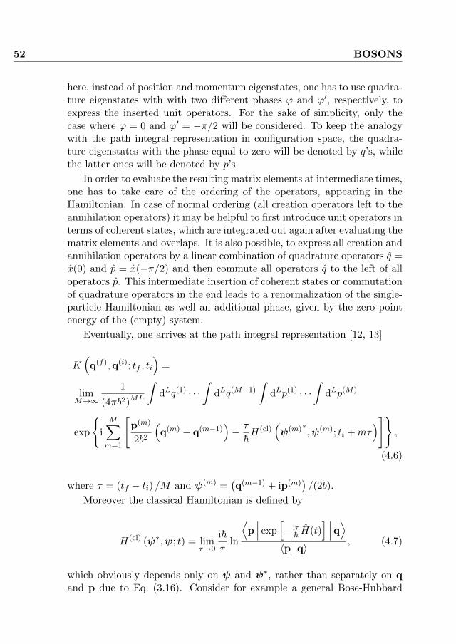
52 BOSONS
here, instead of position and momentum eigenstates, one has to use quadra-ture eigenstates with with two different phases ϕ and ϕ′, respectively, toexpress the inserted unit operators. For the sake of simplicity, only thecase where ϕ = 0 and ϕ′ = −π/2 will be considered. To keep the analogywith the path integral representation in configuration space, the quadra-ture eigenstates with the phase equal to zero will be denoted by q’s, whilethe latter ones will be denoted by p’s.
In order to evaluate the resulting matrix elements at intermediate times,one has to take care of the ordering of the operators, appearing in theHamiltonian. In case of normal ordering (all creation operators left to theannihilation operators) it may be helpful to first introduce unit operators interms of coherent states, which are integrated out again after evaluating thematrix elements and overlaps. It is also possible, to express all creation andannihilation operators by a linear combination of quadrature operators q =x(0) and p = x(−π/2) and then commute all operators q to the left of alloperators p. This intermediate insertion of coherent states or commutationof quadrature operators in the end leads to a renormalization of the single-particle Hamiltonian as well an additional phase, given by the zero pointenergy of the (empty) system.
Eventually, one arrives at the path integral representation [12, 13]
K(q(f),q(i); tf , ti
)=
limM→∞
1
(4πb2)ML
∫dLq(1) · · ·
∫dLq(M−1)
∫dLp(1) · · ·
∫dLp(M)
exp
i
M∑m=1
[p(m)
2b2
(q(m) − q(m−1)
)− τ
hH(cl)
(ψ(m)∗,ψ(m); ti +mτ
)],
(4.6)
where τ = (tf − ti) /M and ψ(m) =(q(m−1) + ip(m)
)/(2b).
Moreover the classical Hamiltonian is defined by
H(cl) (ψ∗,ψ; t) = limτ→0
ih
τln
⟨p∣∣∣ exp
[− iτh H(t)
] ∣∣∣q⟩〈p |q〉 , (4.7)
which obviously depends only on ψ and ψ∗, rather than separately on qand p due to Eq. (3.16). Consider for example a general Bose-Hubbard

4.2. THE QUADRATURE PATH INTEGRAL REPRESENTATION 53
Hamiltonian with two-body interactions,
H =L∑
l1,l2=1
H(0)l1l2a†l1 al2 +
1
2
L∑l1,l2,l3,l4=1
Vl1l2l3l4 a†l1a†l2 al3 al4 , (4.8)
where the coefficients must satisfy
H(0)ll′ = H
(0)l′l
∗
Vl1l2l3l4 = V ∗l4l3l2l1
in order for the Hamiltonian to be hermitian. Moreover, due to the com-mutation relations of the creation and annihilation operators, one is free tochoose the interaction coefficients such that
Vl1l2l3l4 = Vl2l1l3l4 = Vl1l2l4l3 = Vl2l1l4l3 .
In the case of normal ordering, for such a Hamiltonian, one finds the clas-sical limit in quadrature representation to be given by (see App. A.1 fordetails of the derivation)
H(cl) (ψ∗,ψ) =
L∑l1,l2=1
H(0)l1l2
(ψ∗l1ψl2 −
1
2δl1l2
)
+1
2
L∑l1,l2,l3l4=1
Vl1l3l2l4
(ψ∗l1ψl2 −
1
2δl1l2
)(ψ∗l3ψl4 −
1
2δl3l4
).
(4.9)
This example specifically shows that the classical Hamiltonian is not de-termined by just replacing al → ψl and a†l → ψ∗l . In fact, for the generalBose-Hubbard Hamiltonian, Eq. (4.8), the replacement rule would be
a†l al′ → ψ∗l ψl′ −1
2δll′ .
Moreover, note that the classical Hamiltonian also contain constant terms,which give rise to a constant phase in the propagator. Such phases havebeen found on the level of the semiclassical propagator, when using coherentstates as the basis [65–67, 69, 235–238], where they have been denoted asthe Solari-Kochetov extra-phase. It should also be noted that the classicalHamiltonian depends on the chosen ordering of the propagator. Finally,

54 BOSONS
<ψ = 12bq
(i)
<ψ = 12bq
(f)ihψ = ∂H(cl)
∂ψ∗
Figure 4.1: Graphical representation of a trajectory involved in the semi-classical propagator in quadrature representation.
the boundary conditions of the path integral are given by q(0) = q(i) aswell as q(M) = q(f).
It is worth to note that for a Hamiltonian which can be written interms of combinations a†l al′ only, (4.6) is independent of the choice of thequadrature states, as long as the phase difference between the q’s and p’s is−π/2, i.e. when chosing q = x(ϕ) and p = x(ϕ − π/2), the resulting pathintegral representation is independent on the choice of ϕ. This can be seenfrom the expressions of the creation and annihilation operators in termsof quadrature operators, Eq. (3.9), as well as the commutation relationsof the quadratures (3.10) and the overlap of quadrature eigenstates withphase difference π/2, (3.15). Therefore, the following results are valid forany phase ϕ chosen for the quadrature eigenstates q.
4.3 The Semiclassical Propagator in QuadratureRepresentation
4.3.1 Propagator between quadratures with the same phase
Starting from equation (4.6), the semiclassical propagator in quadraturerepresentation is derived, following the steps in section 2.2 by a stationaryphase approximation to the path integral. This yields the many-body van-Vleck-Gutzwiller propagator in quadrature representation, given by
K(q(f),q(i); tf , ti
)=
∑γ:q(i)→q(f)
√det
1
(−2πih)
∂2Rγ(q(f),q(i); tf , ti
)∂q(f)∂q(i)
× exp
[i
hRγ
(q(f),q(i); tf , ti
)].
(4.10)
The trajectories, which can graphically be represented as in Fig. 4.1 are

4.3. THE PROPAGATOR IN QUADRATURE REPRESENTATION 55
given by the equations of motion
ih∂ψ(t)
∂t=∂H(cl) (ψ∗(t),ψ(t); t)
∂ψ∗(t). (4.11)
Furthermore, in (4.10), q(t) and p(t) are the real and imaginary parts ofψ(t), respectively, i.e. ψ(t) = (q(t) + ip(t)) /(2b), where q(t) and p(t) areboth real functions of time. Finally, the boundary conditions are
<ψ (ti) =1
2bq(i),
<ψ (tf ) =1
2bq(f).
(4.12)
Since the boundary conditions in quadrature representation fix the realparts of ψ(ti) and ψ(tf ) only, the overdetermination problem, which arisesin the coherent state representation is solved. The trajectories don’t haveto be complexified, a key advantage of this formulation.
The action along the trajectory can be read from (4.6):
Rγ
(q(f),q(i); tf , ti
)=
tf∫ti
dt
[h
2b2p(t) · q(t)−H(cl) (ψ∗(t),ψ(t); t)
].
(4.13)In the same way as for the single-particle case, the derivatives of the actionwith respect to the boundary conditions can be calculated by using theequations of motion and yield
∂Rγ(q(f),q(i); tf , ti
)∂q
(i)l
= − h
2b2p
(γ)l (ti) ,
∂Rγ(q(f),q(i); tf , ti
)∂q
(f)l
=h
2b2p
(γ)l (tf ) .
(4.14)
Furthermore for a time-independent hamiltonian, the time derivative of theaction is given by
∂Rγ(q(f),q(i); tf , ti
)∂tf
= Eγ ,
where Eγ = H(cl) (ψ∗(ti),ψ(ti)) is the energy of the trajectory.

56 BOSONS
4.3.2 Propagator between quadratures with different phases
Having the propagator in quadrature representation, where the phasesof the initial and final quadrature states are the same also allows to derivethe semiclassical propagator in a mixed basis, for which the initial andfinal quadrature phases are different. However, since (4.10) is valid for anychoice of the quadrature phase (provided, the final one is the same as theinitial one), here only the case of a vanishing initial quadrature phase isconsidered.
The propagator between quadrature states with different phases can berelated to the one between two quadrature states with the same phases byinserting a unity operator in terms of quadrature eigenstates,
K(ϕ)(x(f), tf ; q(i), ti
)=
⟨x(f)
∣∣∣ϕ
T exp
− i
h
tf∫ti
dtH (t)
|q(i)〉
=
∫dq(f)
⟨x(f)
∣∣∣q(f)⟩
ϕK(q(f), tf ; q(i), ti
).
Inserting the overlap of two quadrature eigenstates (3.14a) and the semi-classical propagator (4.10) allows to evaluate the integral in stationaryphase approximation. The stationary phase condition reads
1
sinϕ
[x(f) − q(f) cosϕ
]+ p(γ) (tf ) = 0,
which selects those trajectories satisfying
x(f) = 2b<[ψ(γ) (tf ) exp (iϕ)
].
After expanding the exponential up to second order in q(f) around thisstationary point and computing this integral, the resulting semiclassicalpropagator between two quadratures with different phase is given by
K(ϕ)(x(f), tf ; q(i), ti
)=
∑γ
√det
1
(−2πih)
∂2Rγ
∂q(i)∂x(f)exp
(i
hRγ −
iLϕ
2
),
(4.15)

4.3. THE PROPAGATOR IN QUADRATURE REPRESENTATION 57
where the sum runs over all classical trajectories satisfying the equationsof motion (4.11) as well as the boundary conditions
<ψ (ti) =1
2bq(i)
< [ψ (tf ) exp (iϕ)] =1
2bx(f)
(4.16)
with the classical action is given by
Rγ
(x(f),q(i); tf , ti
)=
h2x(f) · <ψ (tf )−
(x(f)2
+ [<ψ (tf )]2)
cos (ϕ)
4b2 sin (ϕ)
+
tf∫ti
dt[2h=ψ(t) · <ψ(t)−H(cl) (ψ∗(t),ψ(t); t)
].
With this result, by transforming from the initial quadrature with zerophase to a quadrature state with phase ϕ, one could also check again thatthe result for the propagator between two quadrature states with the samephase is independent of ϕ. By evaluating the integration involoved in thistransformation in stationary phase approximation, the boundary conditionsfor the resulting trajectories γ are found to be
x(i/f) = 2b<[ψ(ti/f)
exp (iϕ)],
while the action is given by
Rγ = 2h
tf∫ti
dt= [ψ exp (iϕ)] · <
[ψ exp (iϕ)
]−H(cl) (ψ∗(t),ψ(t); t)
.
The general form is again the same as in (4.10) and also the equations ofmotion are not changed. Due to the invariance of the classical hamiltonianwith respect to the transformation ψ → ψ exp (iβ) for any β, one can alsosubstitute ψ by φ = ψ exp (iϕ) and recovers (4.10).
4.3.3 An initial value representation using quandratures
The semiclassical propagator as a shooting problem, i.e. given by a sumover trajectories fixed by an initial and final conditions such as Eq. (4.12),

58 BOSONS
has proofed very successful to describe interference effects [19–25, 31, 32,34–37, 39–41, 43, 47–54]. However, especially when considering a specificsystem without wanting to impose a disorder average, it is a very hard task,to find all these trajectories.
Although there are in principle methods to do this root search nu-merically [239–246] based on the Newton-Raphson root search method[246, 247], it might be advantageous to have an initial value representa-tion of the propagator, i.e. a representation along the lines of Hermanand Kluk [70], where the initial value of ψ(t) is completely fixed and thenevolved under the classical equations of motion, which is finally iteratedover different initial conditions.
To find such an initial value representation, consider an arbitrary initialstate |ψi〉 which is evolved quantum mechanically in time, such that thefinal state is given by
|ψ (tf )〉 = K (tf , ti) |ψi〉
=
∫dLq(f)
∫dLq(i)
∣∣∣q(f)⟩⟨
q(f)∣∣∣ K (tf , ti)
∣∣∣q(i)⟩⟨
q(i)∣∣∣ψi⟩ .
In the second line this final state has been written in a form, such that thesemiclassical propagator in quadrature representation, Eq. (4.10), can beinserted directly. Using furthermore Eq. (4.14) in order to transform thesemiclassical prefactor into a derivative of the initial imaginary part of themean field wave function, p(γ) (ti) with respect to the final real part, q(f),yields
|ψ (tf )〉 =∫dLq(f)
∫dLq(i)
∣∣∣q(f)⟩⟨
q(i)∣∣∣ψi⟩ ∑
γ:q(i)→q(f)
√det
1
4iπb2∂p(γ) (ti)
∂q(f)
× exp
[i
hRγ
(q(f),q(i); tf , ti
)].
Finally, the sum over classical trajectories can be transformed into an in-tegral over the initial imaginary part according to∑γ:q(i)→q(f)
=
∫dLp(i)δ
[q(q(i),p(i); tf
)− q(f)
] ∣∣∣∣∣det∂q(q(i),p(i); tf
)∂p(i)
∣∣∣∣∣ ,with q
(q(i),p(i); tf
)being the real part of the classical time evolution of
the initial state q(i) + ip(i). The integration over q(f) can now be carried

4.4. THE PROPAGATOR IN FOCK STATE REPRESENTATION 59
out easily due to the Dirac delta and yields the initial value representationin quadrature representation,
|ψ (tf )〉 =
∫dLq(i)
∫dLp(i)
√det
1
4iπb2∂q (tf )
∂p(i)
⟨q(i)
∣∣∣ψi⟩ |q (tf )〉
× exp
[i
hR(q(i),q(f); tf , ti
)].
(4.17)
The square root depends only on the derivative of the final real part ofthe mean field trajectory with respect to the initial imaginary part andis therefore much easier to compute than the determinant arising in theHerman-Kluk propagator [70]. However, to be honest, Eq. (4.17), has anumerical disadvantage when compared to the Herman-Kluk propagator.This lies in the fact that the integration over p(i) runs over the whole RL,without any weight function, which prevent an efficient computation of theintegral by monte carlo methods [247].
4.4 The Semiclassical Propagator in Fock StateRepresentation
4.4.1 The propagator
For ultra-cold atoms, the experimental preparation of a quadratureeigenstate is not possible, since these states are a superposition of all possi-ble Fock states and therefore of states with different total particle numbersN [234]. Therefore it is important to have a propagator in Fock state rep-resentation. A direct derivation of a path integral representation in Fockstate representation, however is not possible, since at intermediate times,one would need a resolution of unity given by an integral, rather than asum.
To avoid this problem, one can use the semiclassical propagator inquadrature representation and project it to Fock states via
K(n(f),n(i); tf , ti
)= 〈n(f)| K (tf , ti) |n(i)〉
=
∫dLq(f)
∫dLq(i)
⟨n(f)
∣∣∣q(f)⟩K(q(f),q(i); tf , ti
)⟨q(i)
∣∣∣n(i)⟩.

60 BOSONS
The integrals can easily be evaluated within the stationary phase approxi-mation, after the overlap of the quadrature eigenstates with Fock states isapproximated by its asymptotic formula, (3.13). However, there is a subtledetail, which complicates the evaluation. This is due to the U(1)-gaugeinvariance, i.e. the fact that if ψ(t) solves the equations of motion, ψ(t)eiθ
also does, implying that the global phase does not play any role, but onlythe phase differences of the components of ψ matter. This also reflectsitself in the classical Hamiltonian, where the phases itself do not enter,but the phase differences do. Obviously, θ is a cyclic variable, implying anadditional constant of motion. This constant of motion, on the other handis obvious: the total number of particles N .
The presence of the gauge freedom implies that there is a continuousfamily of trajectories, for which |ψl(ti)|2 is the same, and since the station-ary approximation breaks down in the presence of such continuous familiesof trajectories, the integral over the global phase θ has to be done exactly,leaving only 2L − 1 integrals to be done in stationary phase approxima-tion. After evaluating these integrals (see appendix A.3 for details), thepropagator in Fock state representation is found to be given by
K(n(f),n(i); tf , ti
)=
∑γ:n(i)→n(f)
√det′
1
(−2πih)
∂2Rγ(n(f),n(i); tf , ti
)∂n(f)∂n(i)
× exp
[i
hRγ
(n(f),n(i); ti, tf
)]δN(i),N(f) ,
(4.18)
where
N (i) =L∑l=1
n(i)l ,
N (f) =
L∑l=1
n(f)l
is the total number of particles at initial and final time, respectively. Thetrajectories, which are schematically depicted in Fig. 4.2, here are deter-mined by the equations of motion (4.11) as well as the boundary conditions
|ψl (ti)|2 = n(i)l +
1
2,
|ψl (tf )|2 = n(f)l +
1
2
(4.19)

4.4. THE PROPAGATOR IN FOCK STATE REPRESENTATION 61
γ1
γ2
γ3
ψ(γ1)(t) =(√
52eiθ1 ,
√52eiθ2 ,
√12eiθ3 ,
√72eiθ4 ,
√12eiθ5)
ψ(γ2)(t) =(√
2eiθ1 ,√
2eiθ2 ,√
56eiθ3 ,
√72eiθ4 ,
√76eiθ5)
ψ(γ3)(t) =(√
52eiθ1 ,
√72eiθ2 , eiθ3 ,
√43eiθ4 ,
√56eiθ5)
Figure 4.2: Illustration of the classical trajectories. While at initial andfinal time, the occupation number have to be integer, this needs not betrue at intermediate times. The total number of particles N =
∑α |ψα(t)|2,
however, stays constant along the classical trajectories.
where one of the initial phases, say the initial phase of the i = 1-component,of ψ has to be fixed to a certain value. Due to the gauge invariance, thetrajectories and the action do not depend on the value of this phase. Finally,the prime at the determinant in Eq. (4.18) indicates that the derivative hasto be taken only with respect to the subspace resulting from skipping thecomponent, for which the initial phase has been fixed. This is a consequenceof the conservation of the total number of particles.
The action in (4.18) is given by
R(n(f),n(i); tf , ti
)=
tf∫ti
dt[hθ(t) · n(t)−H(cl) (ψ∗(t),ψ(t))
], (4.20)
where θl(t) and nl(t) are the real variables given by the phase and themodulus of ψl(t), i.e.
ψl(t) =
√nl(t) +
1
2exp (iθl(t)) .
The integral has again to be calculated along the classical trajectory. Simi-lar to the derivative of the action in quadrature representation with respectto q(i) and q(f), the derivatives of the action in Fock state representation

62 BOSONS
with respect to n(i) and n(f) are
∂Rγ(n(f),n(i); ti, tf
)∂n
(i)l
= −hθ(γ)l (ti) ,
∂Rγ(n(f),n(i); ti, tf
)∂n
(f)l
= hθ(γ)l (tf ) .
(4.21)
4.4.2 The (approximate) semi-group property
An important property of the propagator is the semi-group property,Eq. (2.8). It can be shown that the van-Vleck-Gutzwiller propagator satis-fies it when integrals are evaluated in stationary phase approximation [15].Therefore, one might expect that the semi-group property holds for thesemiclassical Propagator in Fock basis as well, within a stationary phaseapproximation.
However, in Fock space, the right hand side of the semi-group propertyis given by a sum over Fock states, rather than an integral,
K(n(f),n(i); tf , ti
)=∑m
(N)K(n(f),m; tf , t0
)K(m,n(i); t0, ti
),
(4.22)such that the stationary phase approximation is not directly applicable.Here, the superscript (N) to the sum indicates that it runs only over thoseoccupations with the total number of particles being equal to N . Thisrestriction is possible, since the propagator is non-zero only if the initialand final total number of particles are the same.
In order to be able to apply a stationary phase approximation, one firstof all has to transform the summation over the intermediate occupations minto an integration. This is usually done by Poisson summation. However,here the additional condition
∑αmα = N does not allow a direct applica-
tion of the Poisson sum formula. Instead, one can introduce an integrationby hand, e.g. by replacing the sum over Fock states according to∑
m∈NLδN(f),Nm
δNm,N(i) . . . =
∑m∈NL−1
δN(f),N(i)
∞∫0
dLkL∏l=2
δ(ml − k′l
)δ(Nk −N (i)
). . .

4.4. THE PROPAGATOR IN FOCK STATE REPRESENTATION 63
The sum over occupations on the right hand side, is now restricted to thesingle-particle states 2, . . . , L. In the same way, k′ is defined as the vectorresulting from k by removing its first entry. Moreover,
Nm =
L∑l=1
ml.
is the total number of particles of the Fock state |m〉.Still, the Dirac delta does not allow for a stationary phase approxima-
tion, and thus one has to get rid of it. This is possible by applying thePoisson summation,
∞∑m=0
f(m) =
∞∑j=−∞
∞∫0
dmf(m) exp (2πimj) ,
to the sum over occupations. The evaluation of the resulting integral overm is then straight forward and yields, after insertion of the semiclassicalpropagator, Eq. (4.18), for the right hand side of the semi-group property
δN(f),N(i)
∑j∈ZL−1
∞∫0
dLkδ(Nk −N (i)
)(2πih)L−1
exp(2πij · k′
)×
∑γ:n(i)→kγ′:k→n(f)
√det′
∂2Rγ′
∂k∂n(f)det′
∂2Rγ
∂n(i)∂kexp
i
h
[Rγ′ +Rγ
].
The k1-integration of course can be carried out exactly, while the remain-ing L− 1 k-integrals will be evaluated in stationary phase approximation.Before doing so, it is convenient to replace the trajectory γ′ by γ∗ with theinitial phase of the first component θγ∗,1(t0) = θγ,1(t0), i.e. by a trajectorywhich initial phase of the first component is the same as the final one of γ.This replacement can be done by simply multiplying ψγ′(t) with a globaland time-independent phase. The stationarity condition for the integrationover kl with l ∈ 2, . . . , L then reads
−θγ∗,l(t0) + θγ,l(t0) + 2πjl = 0.
Here it is important to notice that θγ∗,l(t0) ∈ [−π, π], while in principleθγ,l(t0) ∈ R. Thus the term 2πjl corrects the discrepancy between the finalphase of the trajectory γ and the initial one of the trajectory γ∗, i.e. if
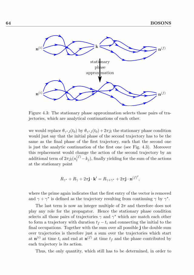
64 BOSONS
n(i) kn(f)
stationaryphase
approximation
n(i) n(f)
Figure 4.3: The stationary phase approximation selects those pairs of tra-jectories, which are analytical continuations of each other.
we would replace θγ∗,l(t0) by θγ∗,l(t0) + 2πjl the stationary phase conditionwould just say that the initial phase of the second trajectory has to be thesame as the final phase of the first trajectory, such that the second oneis just the analytic continuation of the first one (see Fig. 4.3). Moreoverthis replacement would change the action of the second trajectory by an
additional term of 2πjl(n(f)l −kj), finally yielding for the sum of the actions
at the stationary point
Rγ∗ +Rγ + 2πj · k′ = Rγ+γ∗ + 2πj · n(f)′,
where the prime again indicates that the first entry of the vector is removedand γ + γ∗ is defined as the trajectory resulting from continuing γ by γ∗.
The last term is now an integer multiple of 2π and therefore does notplay any role for the propagator. Hence the stationary phase conditionselects all those pairs of trajectories γ and γ∗ which are match each otherto form a trajectory with duration tf − ti and connecting the initial to thefinal occupations. Together with the sum over all possible j the double sumover trajectories is therefore just a sum over the trajectories which startat n(i) at time ti and end at n(f) at time tf and the phase contributed byeach trajectory is its action.
Thus, the only quantity, which still has to be determined, in order to

4.4. THE PROPAGATOR IN FOCK STATE REPRESENTATION 65
check the semi-group property is the functional determinant,
det′∂2Rγ∗
∂k∂n(f) det′∂2Rγ∂n(i)∂k
det∂2(Rγ∗+Rγ+2πj·k′)
∂k′2
To this end, consider the derivative of the stationary phase condition with
respect to n(i)l for l ∈ 2, . . . , L,
d(−θ′γ∗(t0) + θ′γ(t0) + 2πj
)dn(i)′
=∂θ′γ(t0)
∂n(i)′+∂[−θ′γ∗(t0) + θ′γ(t0)
]∂k′
∂k′
∂n(i)′
= 0.
Therefore,
det′∂2Rγ∗
∂k∂n(f) det′∂2Rγ∂n(i)∂k
det∂2(Rγ∗+Rγ+2πj·k′)
∂k′2
= −det
∂θ′γ∗ (tf )
∂k′∂θ′γ(t0)
∂n(i)′
det∂θ′γ(t0)
∂n(i)′∂n(i)′
∂k′
=∂θ′γ∗(tf )
∂n(i)′.
Thus, also the functional determinant is the same as the one of the fullsemiclassical propagator, which finally proofs the validity of the semi-groupproperty, Eq. (4.22), for the semiclassical propagator in Fock basis withina stationary phase approximation.


CHAPTER 5Fermions
As in the bosonic case, the quantity of interest in this chapter is first ofall a semiclassical approximation to the propagator for Fermionic fields inFock state representation,
K(n(f),n(i); tf , ti
)= 〈n(f)| T exp
− i
h
tf∫ti
dtH(t)
|n(i)〉 ,
where the entries of n(i/f) are either zero or one. For later reference, we
define l(i)1 , . . . , l
(i)
N(i) to label those single-particle states which are initially
occupied, and l(f)1 , . . . , l
(f)
N(f) those single-particle states, which are finallyoccupied, i.e.
n(i)l =
1 if l ∈
l(i)1 , . . . , l
(i)
N(i)
0 else
,
n(f)l =
1 if l ∈
l(f)1 , . . . , l
(f)
N(f)
0 else
.
Note that here the L single-particle states are defined to also include the
spin component σ ∈ ↑, ↓. The definition of the labels l(i/f)1 , . . . , l
(i/f)
N(i) isalso illustrated graphically in Fig. 5.1
The main complication for Fermions is that quadrature eigenstates withreal eigenvalues can not be defined, since the occupation numbers can only
67

68 FERMIONS
Figure 5.1: Definition of the labels l(i/f)1 , . . . , l
(i/f)
N(i) as the initially and finallyoccupied single-particle states. Note that here, the ordering of the single-particle states has been chosen such that the spin-up states come first withthe spatial states in ascending order and after that the spin-down states indescending order.
be zero or one. Therefore, one needs to find a different approach comparedto the bosonic case in order to find a semiclassical approximation to thepropagator.
Finally, here for the sake of simplicity, only Hamiltonians of the form
H =L∑
l,l′=1
(hll′ c
†l cl′ + Ul,l′ c
†l c†l′ cl′ cl
).
will be considered.
5.1 The Propagator using Klauder’s CoherentState Representation
5.1.1 The Path Integral
Klauder’s intention with his fermionic coherent state analogue, as re-viewed in §3.3.2, was to determine a path integral for the fermionic propa-gator based on complex variables [231]. However, in his work he consideredonly one single-particle state and considered the propagator in the Klauder-coherent state basis, rather than the Fock basis.
This section aims to generalize his idea to L single-particle states, andto perform a semiclassical approximation to the resulting path integral.However, as will be demonstrated later on, this semiclassical limit risessevere problems.
Being interested in the path integral representation of the propagatorin Fock basis, one needs the representation of the initial and final Fock

5.1. THE PROPAGATOR USING KLAUDER’S REPRESENTATION69
state in Klauder coherent states,
|n(i)〉 =1
πL
1∫0
dLJ (i)
2π∫0
dLθ(i)
L∏l=1
(1− J (i)
l
) 1−n(i)l
2b(i)l
n(i)l
|b(i)〉
with b(i)l =
√J
(i)l exp
(iθ
(i)l
). In view of the semiclassical approximation,
and problems that would arise there otherwise, for the final Fock state theintegration over the amplitudes of b(f) will be performed exactly, such thatthe representation
〈n(f)| =(
1
2π
)L 2π∫0
dLθ(f) exp
(−i
L∑l=1
n(f)l θ
(f)l
)〈b(f)|
with b(f)l = n
(f)l exp
(iθ
(f)l
)will be used. This is because if the same rep-
resentation is used for the final Fock state as for the initial one and allintegrals would be performed in stationary phase approximation, the re-sulting semiclassical approximation diverges.
In a way, this mixed way of representing the initial and final Fock states,is in accordance with the derivation of the semiclassical propagator in con-figuration space, where there is one integration more over the momentathan over the positions.
With this, the propagator in fermionic Fock space can be written as
K(n(f),n(i); tf , ti
)= 〈n(f)| T exp
− i
h
tf∫ti
dtH (t)
|n(i)〉 =
2π∫0
dLθ(f)
πL
1∫0
dLJ (i)
2π∫0
dLθ(i) 〈b(f)| T exp
− i
h
tf∫ti
dtH (t)
|b(i)〉
×L∏l=1
(1− J (i)
l
) 1−n(i)l
2J
(i)l
n(i)l2 exp
[i(n
(i)l θ
(i)l − n
(f)l θ
(f)l
)].
In order to derive a path integral representation, one now follows the stepspresented in section 2.1, but now the unit operators are inserted in termsof Klauder coherent states, Eq. (3.22). Here, in order to evaluating theresulting overlaps and matrix elements it is convenient to assume that the

70 FERMIONS
paths contributing to the path integral are continuous [248], such thatEqns. (3.23) and (3.24) can be applied. This yields for the path integral
K(n(f),n(i); tf , ti
)=
limM→∞
1
2L
1∫0
dLJ (0)
2π∫0
dLθ(0)
πL· · ·
1∫0
dLJ (M)
2π∫0
dLθ(M)
πL
2π∫0
dLθ(M+1)
πL
exp
M∑m=0
(b(m+1)∗ − b(m)∗
)b(m) − b(m+1)∗ (b(m+1) − b(m)
)2
×
L∏l=1
(1− J (0)
l
) 1−n(i)l
2(b(0)l
∗)n(i)l
exp(
in(f)l θ
(M+1)l
)× exp
[− iτ
h
M∑m=0
H(cl)(b(m+1)∗,b(m); tm
)],
with the boundary condition
b(M+1)l = J
(M+1)l exp(iθ
(M+1)j )
and the classical Hamiltonian
H(cl)(b(m+1)∗,b(m); tm
)= 〈b(m+1)| H(tm) |b(m)〉 ,
is evaluated using Eq. (3.24) neglecting the differences between b(m) andb(m+1).
By substituting θ(m)l → θ
(m)l + θ
(0)1 , the initial phase of the first single-
particle state can be integrated out exactly yielding a factor 2πδN(i)N(f) ,while the remaining integrals can be performed in a stationary phase ap-proximation.
5.1.2 Stationary phase approximation
However, it turns out that the resulting semiclassical propagator ob-tained using Klauder’s representation shows severe problems, which makeit inapplicable. Therefore, here only the result of the stationary phase ap-proximation will be presented, in order to discus the problems. Due to thisinapplicability, the results will not be not discussed furthermore.

5.1. THE PROPAGATOR USING KLAUDER’S REPRESENTATION71
Readers interested in details of the stationary phase approximation arereferred to section 5.2.2, where a semiclassical approximation, which ispretty similar to the one using Klauder’s coherent states, will be discussedin detail.
First of all, the stationarity conditions in the continuous limit τ → 0read
ih∂b(t)
∂t=∂H(cl)
(b†(t),b(t); t
)∂b†(t)
as well as
|bl(ti)|2 = n(i)l .
Together with the boundary condition
|bl(tf )|2 = n(f)l
already fixed by the path integral. The stationary phase condition selectsmean then field trajectories connecting the initial to the final occupations.
Note that the additional factors
(1− J (0)
l
) 1−n(i)l
2(J
(0)l
)n(i)l2
have not been included in the stationarity analysis and are equal to unity,when evaluated at the stationary point.
Here, we already observe a first severe problem: In order to derive theclassical limit from the path integral, the off-diagonal terms of the classicalHamilontian are obtained by replacement
c†l cl′ → b∗l bl′
√(1−
∣∣bl∣∣2)(1− |bl′ |2).
Then, inserting the initial condition |bl| = n(i)l immediately shows that the
off-diagonal terms vanish. Therefore, the resulting semiclassical propagatorcan in general not provide reasonable results, as the classical limit has thephysical Fock states as fixed points.
Let us nevertheless assume that this problem can somehow be lifted,and continue with the semiclassical approximation. After a rather lengthycalculation, performing all limits one can perform, one ends up with the

72 FERMIONS
semiclassical propagator
K(n(f),n(i); tf , ti
)=
limM→∞
2(M+3/2)L∑
γ:n(i)→n(f)
√det
1
(−2πih)
∂2Rγ
∂n(f)∂n(i)exp
(i
hRγ
)
× exp
i
2
L∑l=1
[θl(tf )− θl(ti)] +i
2h
tf∫ti
dtTr∂2H(cl)
∂b†∂b
.Here, we finally observe another severe problem, which is the factor
limM→∞
2(M+3/2)L,
which actually is infinite. Thus, even if we could lift the above problemthat the off-diagonal terms in this approach vanish, the final result wouldbe infinite. This does have sence, however, since the sum over classicaltrajectories vanishes. Nevertheless, since the Fock states are fixed pointsof the classical motion, Klauder’s coherent states seem not to be appli-cable for deriving a semiclassical propagator for Fermions in Fock staterepresentation.
5.2 The Semiclassical Propagator in FermionicFock States
5.2.1 The complex Path Integral for the Propagator in Fock stateRepresentation
It seems then that there is no choice but to use coherent states inorder to evaluate the propagator. The semiclassical approximation for theGrassmann path integral however, would lead to classical Grassmannianequations of motion, which would not be of great help. Therefore, onemay want to somehow replace the integrals over Grassmann variables byones over complex variables. The procedure introduced here may somehowremind to a supersymmetric approach, where the fermions are replaced bytheir bosonic supersymmetric partners.
To carry on this program after using Trotter’s formula between twoconsecutive exponentials not only one unit operator but two are inserted
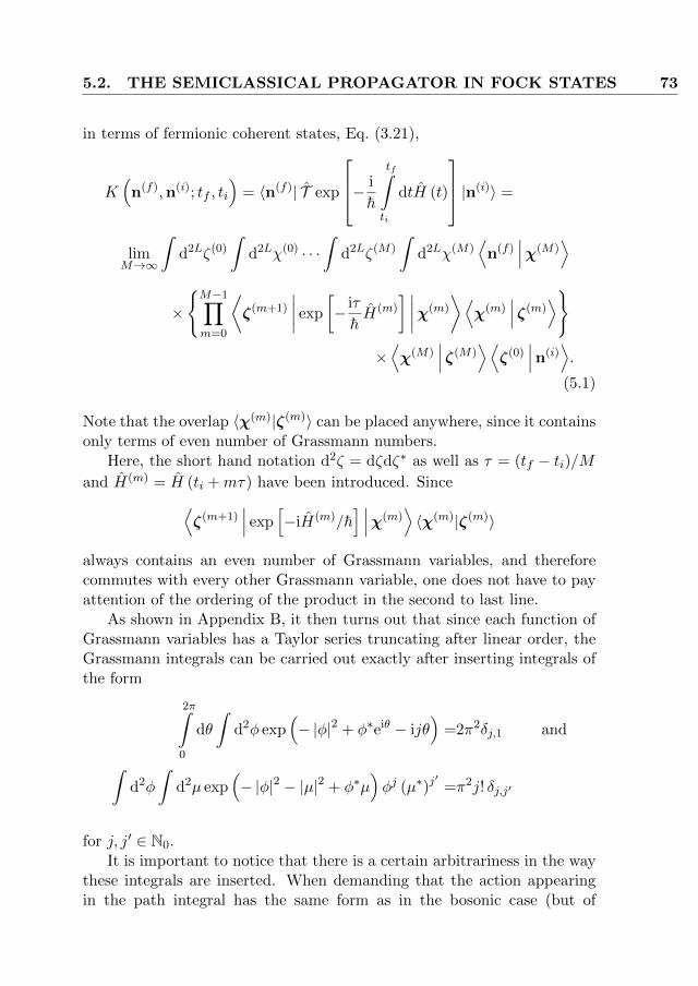
5.2. THE SEMICLASSICAL PROPAGATOR IN FOCK STATES 73
in terms of fermionic coherent states, Eq. (3.21),
K(n(f),n(i); tf , ti
)= 〈n(f)| T exp
− i
h
tf∫ti
dtH (t)
|n(i)〉 =
limM→∞
∫d2Lζ(0)
∫d2Lχ(0) · · ·
∫d2Lζ(M)
∫d2Lχ(M)
⟨n(f)
∣∣∣χ(M)⟩
×M−1∏m=0
⟨ζ(m+1)
∣∣∣∣ exp
[− iτ
hH(m)
] ∣∣∣∣χ(m)
⟩⟨χ(m)
∣∣∣ ζ(m)⟩
×⟨χ(M)
∣∣∣ ζ(M)⟩⟨ζ(0)
∣∣∣n(i)⟩.
(5.1)
Note that the overlap 〈χ(m)|ζ(m)〉 can be placed anywhere, since it containsonly terms of even number of Grassmann numbers.
Here, the short hand notation d2ζ = dζdζ∗ as well as τ = (tf − ti)/Mand H(m) = H (ti +mτ) have been introduced. Since⟨
ζ(m+1)∣∣∣ exp
[−iH(m)/h
] ∣∣∣χ(m)⟩〈χ(m)|ζ(m)〉
always contains an even number of Grassmann variables, and thereforecommutes with every other Grassmann variable, one does not have to payattention of the ordering of the product in the second to last line.
As shown in Appendix B, it then turns out that since each function ofGrassmann variables has a Taylor series truncating after linear order, theGrassmann integrals can be carried out exactly after inserting integrals ofthe form
2π∫0
dθ
∫d2φ exp
(− |φ|2 + φ∗eiθ − ijθ
)=2π2δj,1 and
∫d2φ
∫d2µ exp
(− |φ|2 − |µ|2 + φ∗µ
)φj (µ∗)j
′=π2j! δj,j′
for j, j′ ∈ N0.It is important to notice that there is a certain arbitrariness in the way
these integrals are inserted. When demanding that the action appearingin the path integral has the same form as in the bosonic case (but of

74 FERMIONS
Figure 5.2: For indistinguishable particles, these two processes can not betold apart. However, the right one results from the left one by exchangingthe two particles, which for fermions requires an additional minus sign
course with a different Hamiltonian), this arbitrariness affects the boundaryterms and the classical Hamiltonian only. Here, the choice is such that theclassical Hamiltonian reads
H(cl) (µ∗,φ; tk) =
L∑α=1
h(k)ααµ
∗αφα +
L∑α,β=1α 6=β
U(k)αβ µ
∗αµ∗βφβφα
+L∑
α,β=1α 6=β
h(k)αβµ
∗αφβ exp
(−µ∗αφα − µ∗βφβ
) max(α,β)−1∏l=min(α,β)+1
(1− 2µ∗l φl) .
(5.2)
In Eq. (5.2), the fermionic character is included in the last term, whichdiscribes the hopping from one site α to another one β 6= α,
h(k)αβµ
∗αφβ exp
(−µ∗αφα − µ∗βφβ
) max(α,β)−1∏l=min(α,β)+1
(1− 2µ∗l φl) .
Here, the last factor, which is a product over all sites between α and β,accounts for the anticommutativity, which yields an additional minus signfor each occupied state between the ones, for which the hopping occurs(see Fig. 5.2). This additional minus sign is exactly the one included in thedefinition of the creation (3.3) and annihilation operators (3.4). Moreover,the exponential factor suppresses those hopping events for which the final

5.2. THE SEMICLASSICAL PROPAGATOR IN FOCK STATES 75
occupation number is larger than one accounting effectively for the Pauliexclusion principle. Furthermore, in the classical limit occupations largerthan one are not strictly forbidden. Instead, they are just penalized. How-ever, in Eq. (5.1), only the physical Fock states with occupations 0 or 1 areused, and therefore, only those trajectories with physical initial and finaloccupations will matter, as will become more clearly, when the semiclas-sical limit is considered. Yet, at intermediate times, the occupations maystill be larger than one.
The boundary conditions are chosen such that the path integral is givenby
K(n(f),n(i); tf , ti
)=
limM→∞
2π∫0
dN(i)θ(i)
∫d2Lφ(1) · · ·
∫d2Lφ(M−1)
∫d2N(f)
φ(M)
N(f)∏j=1
φ(M)
l(f)j
exp
M∑m=1
[φ(m)∗ ·
(φ(m−1) − φ(m)
)− iτ
hH(cl)
(φ(m)∗,φ(m−1); tm−1
)]
× 1
(2π)N(i)πN
(f)+(M−1)Lexp
−iN(i)∑j=1
θ(i)
l(i)j
,(5.3)
with φ(0)l = n
(i)l exp
(iθ
(i)l
). This path integral can also be written in a
more common form as,
K(n(f),n(i); tf , ti
)=
2π∫0
dN(i)θ(i)
(2π)N(i)
exp
−i
N(i)∑j=1
θ(i)
l(i)j
∫ d2N(f)φ(f)
πN(f)
N(f)∏j=1
φ(f)
l(f)j
∫D [φ(t)] exp
− i
h
tf∫ti
dt[hJ(t) · θ(t) +H(cl) (φ∗(t),φ(t); t)
]× exp
1
2
(N (i) −
∣∣∣φ(f)∣∣∣2),
where we defined J(t) to be the vector containing the amplitudes of thefield, Jl(t) = |φl(t)|2 and the path integral runs over all paths φ(t) with

76 FERMIONS
the boundary conditions
φl(ti) = n(i)l exp
(iθ
(i)l
)φl(ti) = φ
(f)l
Note that (5.3) results from
K(n(f),n(i); tf , ti
)=∫
dN(i)φ(i)
∫d2N(f)
φ(f)
N(f)∏j=1
φ(f)
l(f)j
N(i)∏j=1
φ(f)
l(i)j
∗ 1
πN(i)+N(f)
∫D [φ(t)] exp
i
h
tf∫ti
dt[−hJ(t) · θ(t)−H(cl) (φ∗(t),φ(t); t)
]× exp
[−1
2
(∣∣∣φ(f)∣∣∣2 +
∣∣∣φ(i)∣∣∣1)],
by integrating out |φ(i)
l(i)j
|2 exactly. These mixed boundary conditions have
been chosen such that for a diagonal non-interacting Hamiltonian, the semi-classical approximation coincides with the exact propagator and thereforecan be understood as a choice for the regularization of the path integral. In-cluding the integration over the amplitudes at initial time in the stationarypoint, would yield an additional factor given by Stirling’s approximation to1!≈
√2π/e, while performing the integrals over the final amplitudes also
exactly would contribute the inverse of this factor.
5.2.2 Semiclassical Approximation
For the evaluation of the integrals in (5.3) it seems to be best to sub-
stitute the real and imaginary part of φ(m)l by the square of its amplitude
J(m)l and its phase θ
(m)l relative to θ
(i)l1
:
φ(m)l =
√J
(m)l exp
[i(θ
(m)l − θ(i)
l1
)].
This is so because after this substitution, the Hamiltonian is independent
of θ(i)
l(i)1
, such that we can integrate out this phase exactly, yielding a factor

5.2. THE SEMICLASSICAL PROPAGATOR IN FOCK STATES 77
2πδN(i),N(f) , which accounts for the conservation of the total number of
particles N = N (i) = N (f). After this integration the value of θ(i)
l(i)1
has to
be fixed, e.g. to zero. For simplicity, in the following we will also define
θ(i)l = 0 ∀l ∈ 1, . . . , L \ l(i)2 , . . . , l
(i)
N(i),θ
(f)l = 0 ∀l ∈ 1, . . . , L \ l(f)
1 , . . . , l(f)
N(i).The remaining details of the stationary phase approximation to the pathintegral will be left to Appendix C, while here we just discuss the resultingsemiclassical propagator.
First of all, after performing the continuous limit, M → ∞ ⇔ τ → 0,the stationary phase conditions select the trajectories given by the equa-tions of motion
ihφ =∂H(cl) (φ∗,φ; t)
∂φ∗. (5.4)
as well as the boundary conditions
|φl (ti)|2 =n(i)l (5.5)
|φl (tf )|2 =n(f)l (5.6)
and φl(i)1
(ti) = 1. Therefore, the semiclassical propagator will again be
given by a sum over Gross-Pitaevskii-like trajectories γ joining the initialand final occupations. The phase of each contribution in this sum is givenby the classical action along the trajectory γ
Rγ =
tf∫ti
dt[hθ(t) · J(t)−H(cl) (φ∗(t),φ(t); t)
], (5.7)
where φl(t) =√Jl(t) exp (iθl(t)).
In the following, matrices, which will be denoted as P(i), P(f), P(i)0 ,
P(f)0 , P(i), P(f), P(i)
0 , P(f)0 , Q(i) and Q(f) will be used. P(i) and P(f)
are defined as the N × L-matrices, which removes those entries of an L-dimensional vector v, which correspond to initially and finally occupiedsingle-particle state, respectively,
P(i/f)v =
vl(i/f)1
vl(i/f)2...
vl(i/f)N
. (5.8)
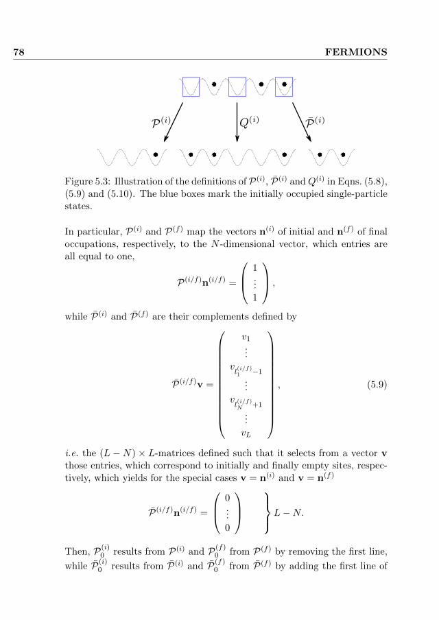
78 FERMIONS
Figure 5.3: Illustration of the definitions of P(i), P(i) andQ(i) in Eqns. (5.8),(5.9) and (5.10). The blue boxes mark the initially occupied single-particlestates.
In particular, P(i) and P(f) map the vectors n(i) of initial and n(f) of finaloccupations, respectively, to the N -dimensional vector, which entries areall equal to one,
P(i/f)n(i/f) =
1...1
,
while P(i) and P(f) are their complements defined by
P(i/f)v =
v1...
vl(i/f)1 −1
...vl(i/f)N +1
...vL
, (5.9)
i.e. the (L −N) × L-matrices defined such that it selects from a vector vthose entries, which correspond to initially and finally empty sites, respec-tively, which yields for the special cases v = n(i) and v = n(f)
P(i/f)n(i/f) =
0...0
L−N.
Then, P(i)0 results from P(i) and P(f)
0 from P(f) by removing the first line,
while P(i)0 results from P(i) and P(f)
0 from P(f) by adding the first line of

5.2. THE SEMICLASSICAL PROPAGATOR IN FOCK STATES 79
P(i), respectively P(f) to P(i), respectively P(f), and the L × L-matricesQ(i) and Q(f) are given by
Q(i/f) =
(P(i/f)
P(i/f)
)(5.10)
That means, they are the (orthogonal) matrices, which move all entries ofn(i/f) equal to zero to the first L − N positions and those, which are oneto the last N positions,
Q(i/f)n(i/f) =
0
L−N...01
N...1
. (5.11)
The definitions of P(i), P(i) and Q(i) are also illustrated graphically inFig. 5.3.
With these definitions, the semiclassical propagator is given by
K(n(f),n(i); tf , ti
)=
∑γ:n(i)→n(f)
exp
(i
hRγ
)K
(γ)red ,
where the amplitude K(γ)red can be shown to read (see Appendix C.1)
K(γ)red =
√detIN + exp
[−2idiag
(P(f)θ (tf )
)]P(f)X (tf )P(f)T
−1
× 1√
2πN−1
exp
i
2h
tf∫ti
dtTr
[∂2H(cl) (φ∗(t),φ(t); t)
∂φ(t)2X(t)
],(5.12)
where X(t) satisfies
X(ti) = Q(i)T
(0
exp[2idiag
(P(i)
0 θ(i))] )Q(i) (5.13a)
X =i
h
∂2H(cl)
∂φ∗2− i
h
∂2H(cl)
∂φ∗∂φX − i
hX∂2H(cl)
∂φ∂φ∗+
i
hX∂2H(cl)
∂φ2 X. (5.13b)

80 FERMIONS
To solve this differential equation for X(t), consider a small perturbation
of the trajectory γ in an initial variable W(i)l (W
(i)l can be e.g. θ
(i)l , J
(i)l ,
φ(i)l or φ
(i)l
∗). The perturbed trajectory γ′, described by φ′ and φ′
∗, which
must be considered as independent variables, can be expanded up to firstorder in the perturbation and is thus written as
φ′l′(t) =φl′(t) + ρl′l(t)W(i)l
φl′∗′(t) =φl′
∗(t) + σl′l(t)W(i)l
The matrices ρ(t) and σ(t) then satisfy the linearized equations of motion
ρ(t) =− i
h
∂2H(cl)
∂φ∗2σ(t)− i
h
∂2H(cl)
∂φ∗∂φρ(t)
σ(t) =i
h
∂2H(cl)
∂φ2 ρ(t) +i
h
∂2H(cl)
∂φ∂φ∗σ(t).
Therefore −ρ(t)σ−1(t) satisfies the same equation of motion as X(t), which
means that we only have to find the variables W(i)l such that σ(ti) is in-
vertible and at the same time X(ti) = −ρ(ti)σ−1(ti). Since φl(t) and φl
∗(t)
are independent variables, this is obtained by the choice Wl(i)j
= θ(i)
l(i)j
for
j = 2, . . . , N and Wl = φl∗(ti) for l /∈ l(i)2 , . . . l
(i)N , i.e.
X(t) = −Q(i)T
∂(P(i)
0 φ(t))
∂(P(i)
0 φ(i)∗) ∂
(P(i)
0 φ(t))
∂(P(i)
0 θ(i))
∂(P(i)
0 φ(t))
∂(P(i)
0 φ(i)) ∂
(P(i)
0 φ(t))
∂(P(i)
0 θ(i))
×
∂(P(i)
0 φ∗(t))
∂(P(i)
0 φ(i)∗) ∂
(P(i)
0 φ∗(t))
∂(P(i)
0 θ(i))
∂(P(i)
0 φ∗(t))
∂(P(i)
0 φ(i)) ∂
(P(i)
0 φ∗(t))
∂(P(i)
0 θ(i))
−1
Q(i)
Finally, the reduced propagator can be further simplified (see AppendixC.2) and the propagator can be written as
K(n(f),n(i); tf , ti
)=
∑γ:n(i)→n(f)
AγBγ exp
(i
hRγ
). (5.14)
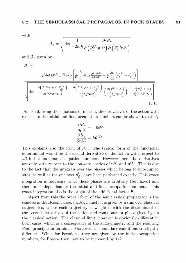
5.2. THE SEMICLASSICAL PROPAGATOR IN FOCK STATES 81
with
Aγ =
√√√√det1
−2iπh
∂2Rγ
∂(P(f)
0 n(f))∂(P(i)
0 n(i)) .
and Bγ given by
Bγ = √detQ(f)Q(i) exp
[i
2h
tf∫ti
dtTr∂2H(cl)
∂φ∂φ∗ + i2
L∑l=1
(θ
(f)l − θ(i)
l
)]√√√√√√det
∂(P(f)φ∗(tf ),J
(f)
l(f)1
)∂(P(i)φ∗(ti))
−∂
(P(f)φ∗(tf ),J
(f)
l(f)1
)∂(P(i)
0 θ(i)) (
∂(P(f)
0 J(f))
∂(P(i)
0 θ(i)) )−1
∂(P(f)
0 J(f))
∂(P(i)φ∗(ti))
.
(5.15)
As usual, using the equations of motion, the derivatives of the action withrespect to the initial and final occupation numbers can be shown to satisfy
∂Rγ
∂n(i)= −hθ(i)
∂Rγ
∂n(f)= hθ(f).
This explains also the form of Aγ . The typical form of the functionaldeterminant would be the second derivative of the action with respect toall initial and final occupation numbers. However, here the derivativesare only with respect to the non-zero entries of n(i) and n(f). This is dueto the fact that the integrals over the phases which belong to unoccupied
sites, as well as the one over θ(i)
ll1have been performed exactly. This exact
integration is necessary, since these phases are arbitrary (but fixed) andtherefore independent of the initial and final occupation numbers. Thisexact integration also is the origin of the additional factor Bγ .
Apart from this the overall form of the semiclassical propagator is thesame as in the Bosonic case, (4.18), namely it is given by a sum over classicaltrajectories, where each trajectory is weighted with the determinant ofthe second derivatives of the action and contributes a phase given by itsthe classical action. The classcial limit, however is obviously different inboth cases, which is a consequence of the antisymmetry and the resultingPauli principle for fermions. Moreover, the boundary conditions are slightlydifferent: While for Fermions, they are given by the initial occupationnumbers, for Bosons they have to be increased by 1/2.


Part III
Interference Effects inBosonic Fock Space
83


CHAPTER 6Non-Interacting Systems
6.1 The Transition Probability for Quadratures
6.1.1 The exact propagator in quadrature representation
For a non-interacting bosonic many-body system, the classical Hamil-tonian in quadrature representation is quadratic,
H(cl)(ψ†,ψ; t
)=
L∑l,l′=1
hll′ψl∗ψl′ . (6.1)
Therefore, the exponential in the path integral (4.6) is also quadratic. Thisin turn means that expanding the exponential up to second order in thevariables which are integrated over, yields again an exact expression, andthe stationary phase approximation is exact.
Hence, for the derivation of the exact propagator in quadrature repre-sentation, one can start from (4.15).
In this case, the equations of motion can be written as
ihψ = Hψ,
where H is the matrix which entries are given by hl,l′ . The solution ofthe equations of motion is given by the (unitary) classical time evolutionoperator
U(t, t′)
= exp
(− i
hH(t− t′
))85

86 NON-INTERACTING SYSTEMS
Figure 6.1: Schematic picture of a waveguide array consisting of six waveg-uides. The energy of a photon is the same in every waveguide as is thehopping amplitude between two neighboring waveguides. The blue arrowssymbolize the entering photons.
applied to ψ (ti), which has to be determined according to the boundaryconditions (4.16) and is given by
ψ (ti) =1
2b
q(i) − i
(U (I)
)−1 [x(f) − U (R)q(i)
],
where U (R/I) are the real/imaginary part of U = U (tf , ti) exp (iϕ). Withinthis chapter, U will also be denoted the effective classical propagator.
After a lengthy but otherwise straightforward calculation, the actionfor this path is found to read
R = − h
4b2
(q(i)
x(f)
)(U (I)
)−1U (R) −
(U (I)
)−1
−[(U (I)
)T]−1
U (R)(U (I)
)−1
( q(i)
x(f)
),
such that finally the exact propagator can be written as

6.1. THE TRANSITION PROBABILITY FOR QUADRATURES 87
K(ϕ)(x(f), tf ; q(i); ti
)=
exp
− i4b2
(q(i)
x(f)
)(U (I)
)−1U (R) −
(U (I)
)−1
−[(U (I)
)T]−1
U (R)(U (I)
)−1
( q(i)
x(f)
)√det
[−4πib2U
(U (I)
)T] .
(6.2)
Having the propagator in the simple form Eq. (6.2), immediately allowsto obtain certain conclusions about the propagation of photons in an wave-guide array as the one shown in Fig. 6.1, if the state of the electromagneticfield is both prepared and measured in a quadrature state.
6.1.2 Propagation between quadratures with the same phase
The result Eq. (6.2) depends on the individual system only via theclassical propagator U(t), which can be computed most efficiently by diag-onalizing the matrix H corresponding to the classical Hamiltonian. Let usdenote the unitary matrix, which diagonalizes H, by O, such that
O†HO = diag (λ) ,
where λ is the vector with entries given by the eigenvalues of H, anddiag (v) is the diagonal matrix with entries given by those of the vector v.Then the classical propagator can be written as
U(t) = O exp
[− i
hdiag (λ) t
]O†.
Here, for real H, i.e. for real hopping parameters hl 6=l′ in Eq. (6.1), some-thing important happens. For a real symmetric matrix, O is a real orthogo-nal matrix, which also implies that it diagonalizes not only H and U(t), butalso the real and imaginary parts of the classical propagator individually,
< [U(t)] = O cos
(λt
h
)OT (6.3)
= [U(t)] = O sin
(λt
h
)OT. (6.4)

88 NON-INTERACTING SYSTEMS
Since the determinant of an orthogonal matrix is always equal to ±1, onesees immediately from Eq. (6.4) that the determinant of U (I) = = [U ] iszero for all times, if at least one eigenvalue of H is zero, and thereforethe propagator seems to diverge. But, the normalization of the propagatordemands that it will actually become a Dirac delta. Indeed, in this caseEq. (6.2) can also be written in the form
K(ϕ)(x(f), tf ; q(i); ti
)=
exp
− i
4b2
[q(i) −
(U (R)
)−1x(f)
](U (I)
)−1U (R)
[q(i) −
(U (R)
)−1x(f)
]
×√
det
[−4πib2U
(U (I)
)T]−1
exp
[i
4b2x(f)U (I)
(U (R)
)−1x(f)
],
which in the case where the determinant of the imaginary part of the ef-fective classical propagator vanishes yields
K(ϕ)(x(f), tf ; q(i); ti
)det U(I)→0−−−−−−−→ 1
det U (R)δ
[q(i) −
(U (R)
)−1x(f)
].
For the case of a (linear) waveguide-array with constant nearest neighborhopping and all the onsite-energies being equal to one another, i.e. for aclassical Hamiltonian given by the matrix
H =
ε −J−J ε −J
. . .. . .
. . .
−J ε −J−J ε
, (6.5)
it is particularly easy to find the condition on the parameters J and ε, forwhich one of the eigenvalues vanishes. For such a matrix, the eigenvaluesare given by
λk = ε+ 2J cos
(kπ
L+ 1
), k = 1, . . . , L,
where L is the number of waveguides. This gives the condition that theon-site energies are given by
ε = −2J cos
(kπ
L+ 1
)(6.6)

6.1. THE TRANSITION PROBABILITY FOR QUADRATURES 89
ϕ=0
ϕ=0.04π
ϕ=0.08π
ϕ=0.12π
-0.7
-0.6
-0.5
-0.4
-0.3
-0.2
-0.1
0
0.1
0 5 10 15 20
det
U~(I
)
t [h/2J]
(a)
-0.5
-0.4
-0.3
-0.2
-0.1
0
0.1
0.2
0.3
0 5 10 15 20
det
U~(I
)
t [h/2J]
(b)
ϕ=0.2π
ϕ=0.3π
ϕ=0.4π
ϕ=0.5π
-0.2
0
0.2
0.4
0.6
0.8
1
0 5 10 15 20
det
U~(I
)
t [h/2J]
(c)
-0.4
-0.2
0
0.2
0.4
0.6
0.8
1
0 5 10 15 20
det
U~(I
)
t [h/2J]
(d)
Figure 6.2: The determinant of the imaginary part of the effective classicalpropagator as a function of time for a linear chain of six wave guides withnearest neighbor hopping J = 0.5 and on-site energies (a), (c) ε = 0 and(b), (d) ε = 0.7 for different phase differences ϕ.
for a k ∈ 1, . . . , L. For an odd number of waveguides, one possiblesolution would be ε = 0.
On the other hand, even if the condition Eq. (6.6) is not fulfilled, thedeterminant of the imaginary part of the classical propagator vanishes forcertain times, which corresponds to the existence of caustics, and thereforeagain the propagator is given by a Dirac delta.
6.1.3 Propagation between quadratures with different phase
The last observation still holds when the phase difference between thequadrature bases used to measure the initial and final state are different.

90 NON-INTERACTING SYSTEMS
Considering again the classical Hamiltonian, Eq. (6.5), yields that
det U (I) =L∏l=1
sin
[ϕ− 1
h
(ε+ 2J cos
lπ
L+ 1
)t
], (6.7)
which holds as the condition on the time for a caustic
tn,l =(nπ + ϕ) h
ε+ 2J cos lπL+1
with n ∈ N. Thus, the phase ϕ shifts the times, at which the caustichappens. This can be seen, when looking at the zeros of det U (I) in Fig. 6.2.It may also happen that for a certain value of ϕ several of these zeroscollapse as for example for ε = 0 and ϕ = 0 as in Fig. 6.2(a).
For ε = 0 it is straightforward to check that the determinant of theeffective classical propagator is symmetric in ϕ around π, which is alsodemonstrated in the left columns of Figs. 6.3, 6.4 and 6.5. This symmetry,however no longer holds for ε 6= 0 (see right columns of Figs. 6.3, 6.4 and6.5). However, when changing ϕ to ϕ + π, the determinant, Eq. (6.7),clearly changes only by an additional sign given by (−1)L.
The general dependence on ϕ and t, however, is not so easy to summa-rize. Fig. 6.2 shows the dime dependence of the determinant for differentvalues of ϕ for a chain consisting of six wave guides with nearest neighbourcoupling J = 0.5, only. As expected, it is a highly oscillatory function oftime, where the height and position of each peak – especially for ε 6= 0 – isstrongly affected by ϕ. To get a better impression on how det U (I) changeswith ϕ, in Figs. 6.3, 6.4 and 6.5, the dependence on ϕ is plotted for differentpropagation times.
Depending on the propagation time, in some cases det U (I) as a functionof ϕ shows two peaks, which are more pronounced than the others, as inFigs. 6.3(a), 6.3(b), 6.3(c), 6.3(d), 6.4(e) and 6.4(f). In other cases, it showsseveral peaks of almost the same heights as in Figs. 6.3(e), 6.3(f), 6.5(c)and 6.5(d).
6.2 The Transition Probability in CoherentStates
The exact propagator for a non-interacting system in coherent staterepresentation can be found by relating it - by inserting unit operators in
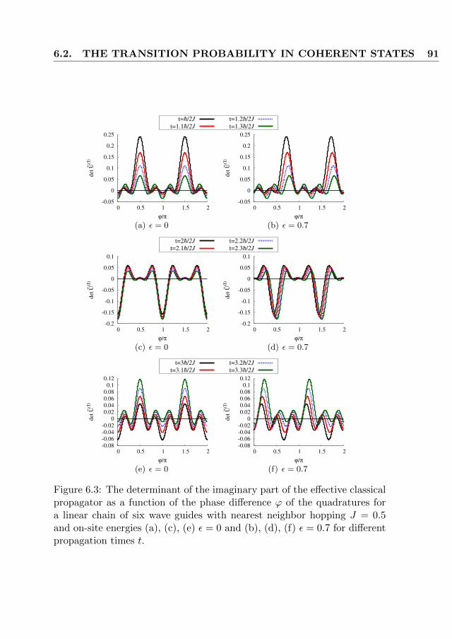
6.2. THE TRANSITION PROBABILITY IN COHERENT STATES 91
t=h/2J
t=1.1h/2J
t=1.2h/2J
t=1.3h/2J
-0.05
0
0.05
0.1
0.15
0.2
0.25
0 0.5 1 1.5 2
det
U~(I
)
ϕ/π
(a) ε = 0
-0.05
0
0.05
0.1
0.15
0.2
0.25
0 0.5 1 1.5 2
det
U~(I
)
ϕ/π
(b) ε = 0.7
t=2h/2J
t=2.1h/2J
t=2.2h/2J
t=2.3h/2J
-0.2
-0.15
-0.1
-0.05
0
0.05
0.1
0 0.5 1 1.5 2
det
U~(I
)
ϕ/π
(c) ε = 0
-0.2
-0.15
-0.1
-0.05
0
0.05
0.1
0 0.5 1 1.5 2
det
U~(I
)
ϕ/π
(d) ε = 0.7
t=3h/2J
t=3.1h/2J
t=3.2h/2J
t=3.3h/2J
-0.08
-0.06
-0.04
-0.02
0
0.02
0.04
0.06
0.08
0.1
0.12
0 0.5 1 1.5 2
det
U~(I
)
ϕ/π
(e) ε = 0
-0.08
-0.06
-0.04
-0.02
0
0.02
0.04
0.06
0.08
0.1
0.12
0 0.5 1 1.5 2
det
U~(I
)
ϕ/π
(f) ε = 0.7
Figure 6.3: The determinant of the imaginary part of the effective classicalpropagator as a function of the phase difference ϕ of the quadratures fora linear chain of six wave guides with nearest neighbor hopping J = 0.5and on-site energies (a), (c), (e) ε = 0 and (b), (d), (f) ε = 0.7 for differentpropagation times t.

92 NON-INTERACTING SYSTEMS
t=4h/2J
t=4.1h/2J
t=4.2h/2J
t=4.3h/2J
-0.1
-0.05
0
0.05
0.1
0.15
0.2
0.25
0 0.5 1 1.5 2
det
U~(I
)
ϕ/π
(a) ε = 0
-0.1
-0.05
0
0.05
0.1
0.15
0.2
0.25
0 0.5 1 1.5 2
det
U~(I
)
ϕ/π
(b) ε = 0.7
t=5h/2J
t=5.1h/2J
t=5.2h/2J
t=5.3h/2J
-0.04
-0.02
0
0.02
0.04
0.06
0.08
0.1
0.12
0 0.5 1 1.5 2
det
U~(I
)
ϕ/π
(c) ε = 0
-0.04
-0.02
0
0.02
0.04
0.06
0.08
0.1
0.12
0 0.5 1 1.5 2
det
U~(I
)
ϕ/π
(d) ε = 0.7
t=10h/2J
t=10.1h/2J
t=10.2h/2J
t=10.3h/2J
-0.05
0
0.05
0.1
0.15
0.2
0.25
0.3
0.35
0.4
0.45
0 0.5 1 1.5 2
det
U~(I
)
ϕ/π
(e) ε = 0
-0.05
0
0.05
0.1
0.15
0.2
0.25
0.3
0.35
0.4
0.45
0 0.5 1 1.5 2
det
U~(I
)
ϕ/π
(f) ε = 0.7
Figure 6.4: The determinant of the imaginary part of the effective classicalpropagator as a function of the phase difference ϕ of the quadratures fora linear chain of six wave guides with nearest neighbor hopping J = 0.5and on-site energies (a), (c), (e) ε = 0 and (b), (d), (f) ε = 0.7 for differentpropagation times t.

6.2. THE TRANSITION PROBABILITY IN COHERENT STATES 93
t=15h/2J
t=15.1h/2J
t=15.2h/2J
t=15.3h/2J
-0.1
-0.05
0
0.05
0.1
0.15
0.2
0.25
0.3
0.35
0 0.5 1 1.5 2
det
U~(I
)
ϕ/π
(a) ε = 0
-0.1
-0.05
0
0.05
0.1
0.15
0.2
0.25
0.3
0.35
0 0.5 1 1.5 2
det
U~(I
)
ϕ/π
(b) ε = 0.7
t=20h/2J
t=20.1h/2J
t=20.2h/2J
t=20.3h/2J
-0.08
-0.06
-0.04
-0.02
0
0.02
0.04
0.06
0 0.5 1 1.5 2
det
U~(I
)
ϕ/π
(c) ε = 0
-0.08
-0.06
-0.04
-0.02
0
0.02
0.04
0.06
0 0.5 1 1.5 2
det
U~(I
)
ϕ/π
(d) ε = 0.7
Figure 6.5: The determinant of the imaginary part of the effective classicalpropagator as a function of the phase difference ϕ of the quadratures for alinear chain of six wave guides with nearest neighbor hopping J = 0.5 andon-site energies (a), (c) ε = 0 and (b), (d) ε = 0.7 for different propagationtimes t.
terms of quadratures - to the propagator in quadrature representation (6.2)for ϕ = 0. The resulting integral consists of gaussian integrals only and istherefore easily computed to find
K(φ(f), tf ;φ(i), ti
)= exp
(−1
2
∣∣∣φ(f)∣∣∣2 − 1
2
∣∣∣φ(i)∣∣∣2 + φ(f)∗U (tf , ti)φ
(i)
).
Computing the modulus square of the propagator now yields for the tran-sition probability between two coherent states
P(φ(f),φ(i)
)=∣∣∣K (φ(f), tf ;φ(i), ti
)∣∣∣2= exp
[−∣∣∣φ(f)
∣∣∣2 − ∣∣∣φ(i)∣∣∣2 + 2<
(φ(f)∗U (tf , ti)φ
(i))].

94 NON-INTERACTING SYSTEMS
Obviously, in contrast to the transition probability between quadratures,the transition probability between coherent states is not constant but de-pends strongly on the chosen initial and final coherent state.
In particular, it is strongly enhanced when
φ(f) = U (tf , ti)φ(i),
namely at the classcial solution.

CHAPTER 7Many-Body Coherent
Backscattering
7.1 Chaotic Regime
The object of interest in this section is the transition probability froman initial Fock state n(i) to a final one n(f),
P(n(f), tf ; n(i), ti
)=∣∣∣〈n(f)| K (tf , ti) |n(i)〉
∣∣∣2 =∣∣∣K (n(f), tf ; n(i), ti
)∣∣∣2 ,i.e. the probability to measure the Fock state n(f) at time tf , if the system
was prepared in the Fock state n(i) at the initial time ti. Here K (tf , ti) =
T exp[−i∫ tfti
dtH (t) /h]
is the quantum mechanical propagator.
Inserting the semiclassical propagator (4.18), yields for the transitionprobability a double sum over trajectories,
P(n(f), tf ; n(i), ti
)≈∑
γ,γ′:n(i)→n(f)
√det′
∂2Rγ
∂n(f)∂n(i)
√det′
∂2Rγ′
∂n(f)∂n(i)
∗exp
[ih
(Rγ −Rγ′
)](2πh)L−1
.(7.1)
In general, one can not say much about the contributions of the doublesums. However, under disorder average, i.e. an average over the on-siteenergies εl = hll, due to the scaling of the action with the total number
95

96 MANY-BODY COHERENT BACKSCATTERING
n(i)n(f)
Figure 7.1: In the diagonal approximation, only identical pairs of trajecto-ries are taken into account
of particles, the action difference in the exponential gives rise to strongoscillations. Most contributions to the double sum cancel out on disorderaverage, unless the two actions for trajectories γ and γ′ are correlated.
7.1.1 Diagonal approximation
The most obvious pairs of trajectories, which are correlated, are theidentical ones, i.e. γ = γ′ (see Fig. 7.1). For those pairs, the action differ-ence is obviously zero and the transition probability in diagonal approxi-mation reduces to
P (da)(n(f), tf ; n(i), ti
)=
1
(2π)L−1
∑γ
∣∣∣∣det′∂θ (ti)
∂n(f)
∣∣∣∣ ,where θ (ti) is the vector containing the initial phases for the trajectory γ.
By inserting an integration over the initial phases together with a Diracdelta, ensuring that only those phases contribute which match the onesgiven by the trajectories and using the properties of the delta function, onecan prove the sum rule
∑γ
∣∣∣∣det′∂θ (ti)
∂n(f)
∣∣∣∣ =
2π∫0
dL−1θ(i)L∏l=2
δ
[∣∣∣ψl (n(i);θ(i); tf
)∣∣∣2 − 1/2− n(f)l
]= (2π)L−1 P (cl)
(n(f), tf ; n(i), ti
),
(7.2)
with ψ(n(i);θ(i); tf ) being the classical time evolution of the initial state
ψ(i) with components
ψ(i)l =
√n
(i)l + 1/2 exp(iθ
(i)l ).
Therefore, the diagonal approximation yields the classical transition prob-ability
P (da)(n(f), tf ; n(i), ti
)= P (cl)
(n(f), tf ; n(i), ti
).

7.1. CHAOTIC REGIME 97
n(f) = n(i)
Figure 7.2: Trajectory pairs responsible for coherent backscattering
7.1.2 Coherent backscattering contribution
An other class of correlated pairs of trajectories are those shown inFig. 7.2, namely γ′ = T γ , where T denotes time reversal. For Bose-Hubbard systems, time reversal is achieved by complex conjugation, suchthat the time reversal of a solution φ (t+ ti) of the equations of motion isφ (tf − t)∗. Of course, these pairs exist only if the Hamiltonian itself is timereversal symmetric, which for a Bose-Hubbard system corresponds to a realHamiltonian. It turns out that a Bose-Hubbard chain with nearest neighborhopping only is always time reversal symmetric, since it can be transformedinto a real one by multiplying each component of the wave function witha certain time-independent phase. In the same way, for certain combina-tions of the phases of the hopping parameter in a Bose-Hubbard ring, theHamiltonian can be transformed into a real one.
Having identified the time reversed of a trajectory γ, it is straightfor-ward to check that the actions of both trajectories are the same,
RT γ = Rγ .
However, in (7.1) pairing γ with its time reversed is possible only, if n(f) =n(i). Therefore, one first has to replace γ and γ′ by nearby trajectories γand γ′, which both start and end at n(0) =
(n(i) + n(f)
)/2. In the course
of this replacement, one also has to expand the actions in n(f) and n(i) upto linear order around n(0),
Rγ −Rγ′ ≈ Rγ −Rγ′ + h(θγ (tf )− θγ′ (tf )
)·(n(f) − n(0)
)−h(θγ (ti)− θγ
′(ti))·(n(i) − n(0)
).

98 MANY-BODY COHERENT BACKSCATTERING
0
0.01
0.02 (d)
0
0.01
0.02 (b)
0
0.01
0.02
pro
bab
ilit
y
(c)
0
0.01
0.02 (a)
0
0.01
0.02 (e)
22
33
42
23
43
22
43
32
32
34
23
24
32
33
24
23
34
22
34
23
23
43
22
42
33
24
32
32
43
32
32
23
43
22
43
32
32
43
23
42
32
42
33
24
32
33
22
43
32
42
33
42
23
42
23
34
23
23
43
22
42
23
34
23
23
42
33
24
32
23
43
23
24
33
22
final state
0
0.01
0.02 (f)
Figure 7.3: Emergence of the coherent backscattering for a Bose-Hubbardchain with five sites from numerical calculations. The initial occupationwas chosen to be (3, 2, 3, 4, 2). The red crosses are the classical transitionprobability, while the black diamonds are the quantum ones. The evolutiontimes are (a) t = 1.5h/J , (b) t = 2.5h/J , (c) t = 5h/J , (d) t = 10h/J , (e)t = 20h/J , (f) t = 50h/J , where J is the hopping parameter. Figure bycourtesy of Julien Dujardin, Arturo Arguelles and Peter Schlagheck.
In the prefactor one can simply replace the second derivative of the actionof the original trajectory by the corresponding one of the new trajectory.
If γ′ is the time reversed of γ, the initial and final phases of γ′ arerelated to those of γ by
θ(γ′) (tf ) =− θ(γ) (ti)
θ(γ′) (ti) =− θ(γ) (tf ) ,
which, after applying the sum rule (7.2), yields for the coherent backscat-tering contribution to the transition probability

7.1. CHAOTIC REGIME 99
P (cbs)(n(f), tf ; n(i), tf
)=
δTRI
(2π)L−1
2π∫0
dL−1θ(i) exp
i[θ(i) + θ
(n(i),θ(i); tf
)]·(n(f) − n(i)
)
×L∏l=2
δ
[∣∣∣ψl (n(i),θ(i); tf
)∣∣∣2 − 1
2− n(i)
],
where δTRI is one, if the system is time reversal invariant and zero other-wise.
For a classically chaotic system, within a disorder average one can re-place the final phases θ(n(i),θ(i); tf ) by identically, independent, in [0, 2π]uniformly distributed random variables, such that for P (cbs) one can per-form an average over the final phases yielding a factor δn(i),n(f) . Thus, theaveraged coherent backscattering contribution to the transition probabilityis given by
P (cbs)(n(f), tf ; n(i), ti
)= δTRIδn(i),n(f)P (cl)
(n(f), tf ; n(i), ti
).
Here, the bar denotes an averaged quantity.As long as time reversal symmetry is the only discrete symmetry of
the system, pairing a trajectory with itself or its time reverse, are theonly two generic possibilities to get a contribution with vanishing actiondifference. All further possible pairs of trajectories give contributions whichare suppressed by a factor of 1/N compared to the two latter. In thesemiclassical limit, the averaged transition probability is then given by
P(n(f), tf ; n(i), ti
)=(
1 + δTRIδn(f),n(i)
)P (cl)
(n(f), tf ; n(i), ti
), (7.3)
i.e. the quantum transition probability is enhanced for n(f) = n(i) com-pared to the classical one by a factor of two due to the constructive inter-ference between time-reversed paths.
However, only paths which are not self-retracing may contribute to thecoherent backscattering peak, because the time reverse of a self-retracingpath is again the path itself and therefore this pairing would already beincluded in the diagonal approximation. For short times, one can expectthat all trajectories coming back to the initial occupations are all self-retracing and therefore a certain minimal time is required to observe co-herent backscattering (see supplementary material of [249]). This behavioras well as the existence of coherent backscattering itself is shown in Fig. 7.3.

100 MANY-BODY COHERENT BACKSCATTERING
223334
232334
233243
233432
242333
322334
323243
323432
332234
332342
333242
334332
343223
423233
432323
4333220
0.004pro
bab
ilit
y(a)
φ = 0
φ = 0.125π
φ = 0.25π
φ = 0.5π
φ = 0, classical
011122
012121
021211
101221
110122
111202
112102
112210
121012
121201
122110
202111
211012
211201
212110
221110
final state
0
0.004
pro
bab
ilit
y
(b)
φ = 0
φ = 0.125π
φ = 0.25π
φ = 0.5π
φ = 0, classical
Figure 7.4: Dependence of the coherent backscattering peak on the phaseφ of the hopping parameter J for a Bose-Hubbard ring consisting of sixsites (see inset of (a)). The initial occupations were chosen to be (a)(3, 3, 2, 3, 4, 2) and (1, 1, 2, 2, 1, 0). Figure by courtesy of Julien Dujardin,Arturo Arguelles and Peter Schlagheck.
Fig. 7.4 shows that the peak indeed vanishes, when time reversal in-variance is broken, which clearly identifies the source of the peak to becoherent backscattering. The fact that for certain phases φ (apart from2π) of the hopping parameter the coherent backscattering peak reappearsis due to the effective reestablishment of time reversal invariance (see [249]).Moreover, Fig. 7.4 shows that – although the semiclassical theory is strictlyspeaking valid for large occupations only, coherent backscattering can beobserved already for very small particle number.

7.1. CHAOTIC REGIME 101
(a) (b)
(c) (d) (e)
(f) (g) (h)
Figure 7.5: Loop diagrams arising in the calculation of the transition prob-ability up to second order. For the one-leg-loops (Diagrams (b), (d), (g))only one of the two possibilities to shift an end into the encounter is shown.Note that for the case of one 2-encounter, there is no no-leg-loop, since theseare already included in the coherent backscattering.
7.1.3 Loop contributions
The result above is expected to be just the leading order result of asemiclassical expansion in action differences. Typically, sub-leading con-tributions arise due to loop diagrams as those shown in Fig. 7.5, whichessentially renormalize the background [21, 33–35, 37, 250, 251].
These loop diagrams consist of encounter regions, where the trajectoriescome close to themselves or their time-reverse, and so called links, whichconnect the encounter regions. Within these links, the two trajectories γand γ′ follow each other or the time-reverse of the other, while within theencounter region both trajectories connect different links. The action dif-ference of the two trajectories then stems solely from the encounter region.
The loop diagrams can be divided into three classes, which are deter-

102 MANY-BODY COHERENT BACKSCATTERING
mined into three groups of loop contributions. The first of which are thetwo leg loops shown in Figs. 7.5(a), 7.5(c) and 7.5(f) for which both thestarting and ending point of the trajectory lies outside the encounter re-gions. For one-leg-loop diagrams, such as Figs. 7.5(b), 7.5(d) and 7.5(g),either the starting or the ending point lies within an encounter region, whilefor no-leg-loops (see Figs. 7.5(e) and 7.5(h)) both the starting and endingpoint lies in the encounter region.
Two leg loops
According to Appendix F, the contribution from two leg loops, i.e. fromthose trajectories for which both the start and the end lie outside of theencounter regions, is given by
P (2ll)(n(f), tf ; n(i), ti
)=
1
(2π)L−1
∑γ:n(i)→n(f)
∣∣∣∣det′∂2Rγ
∂n(f)∂n(i)
∣∣∣∣∑v
N (v)
c∫−c
d(L−2)(O−Nenc)s
c∫−c
d(L−2)(O−Nenc)u
[tf − ti −
∑αoαt
(α)enc (s,u)
]OO! ΩO−Nenc
N
∏αt(α)enc
exp (iNs · u),
(7.4)
where v is the vector which entries vo are the numbers of o-encounters andN (v) is the number of encounter structures with characteristic v, i.e. withvo o-encounters. The total number of links between encounters for twoleg loops, O + 1 =
∑o ovo + 1, as well as the total number of encounters,
Nenc =∑
o vo are uniquely defined by this characteristic.Moreover, the boundary c of the integration over stable and unstable
coordinates, s and u, respectively, is an arbitrary classical bound largecompared to 1/N , but small enough to allow linearization of the partnertrajectory γ′ around γ.
The reduced phase space volume ΩN (E) for constant total number ofparticles N and energy E is defined as
ΩN (E) =
∫d2Lψδ (θ1) δ
(N −
L∑l=1
|ψl|2 +L
2
)δ [H (ψ∗,ψ)− E] .
In principle, in Eq. (7.4), the reduced phase space volume has to be eval-uated at the energy of the trajectory γ. However, on disorder average,

7.1. CHAOTIC REGIME 103
the exact Dirac delta in the energy can be approximated by some broad-ened delta function with an averaged mean energy, such that the resultingreduced phase space volume can be assumed to be independent of the tra-jectory.
Finally, the encounter time t(α)enc, which is the time the trajectory needs,
in order to traverse the α-th encounter once, is the sum of two contributions,
t(α)enc = t(α)
s + t(α)u ,
where ts and tu are given by
t(α)s ∼ 1
λmin
lnc∣∣∣s(α,j)k
∣∣∣ ,
t(α)u ∼ 1
λmin
lnc∣∣∣u(α,j)k
∣∣∣
with λ being the largest Lyapunov exponent. Just as in F, the minimumhere and in the following runs for fixed α over both, the dimensional andsequential, indexes k ∈ 1, . . . , L− 2 and j ∈ 2, . . . , oα.
It has been shown in [32], how to evaluate the integrals in Eq. (7.4) ingeneral: Neglecting higher order as well as on average highly oscillatoryterms, the only contributing term is found by using only the term in the
expansion of the power in the numerator, which contains every t(α)enc exactly
once.
Finally, after substituting
xj = sjuj/c2, σj = c/uj
the integrals, which then run over the domains −1 < xj < 1 and 1 < σj <1/|xj | yield after again identifying the sum over classical trajectories withthe classical transition probability yields [32]
P (2ll)(n(f), tf ; n(i), ti
)=
P (cl)∑v
N (v)(tf − ti)O−Nenc
(O −Nenc) ! ΩO−NencN
(2π
N
)(L−2)(O−Nenc)∏α
(−oα)

104 MANY-BODY COHERENT BACKSCATTERING
One leg loop
The vanishing of one link, in this case does not require further linksto vanish, such that also one leg loop contributions have to be taken intoaccount [45, 252, 253]. Following F.2, the contributions of one leg loopscan be calculated from
P (1ll)(n(f), tf ; n(i), ti
)=
1
(2π)L−1
∑γ:n(i)→n(f)
∣∣∣∣det′∂2Rγ
∂n(f)∂n(i)
∣∣∣∣∑v
∑o1
vo1o1N (v)
O
c∫−c
d(L−2)(O−Nenc)s
c∫0
d(L−2)(O−Nenc)u
tγ−∑αoαt
(α)enc∫
0
dtO
tO∫0
dtO−1 · · ·t3∫
0
dt2
min 1λ
ln c
|sj|∫0
dt′exp (iNs · u)
ΩO−NencN
∏αt(α)enc
,
(7.5)
where now the encounter time is reduced and given by t(1)enc = t′+ t
(1)u . Note
that, although strictly speaking Eq. (7.5) determines the contributions forthose one leg loops, where the starting point lies inside an encounter, thecontribution from trajectories with an ending point lying inside an en-counter is exactly the same. Thus, when finally the higher order contribu-tions to the transition probability are computed, P (1ll) has to be multipliedby a factor of two.
The integrations over the link times t2, . . . , tO as well as those overthe stable and unstable coordinates of the Nenc − 1 encounters, which donot contain the starting point, are exactly the same as above, such that

7.1. CHAOTIC REGIME 105
performing these integrals yields [253]:
P (1ll)(n(f), tf ; n(i), ti
)=
2P (cl)∑v
∑o1
vo1o1N (v)
O
(2π
N
)(L−2)(O−o1−Nenc+1)c∫−c
d(L−2)(o1−1)s
c∫−c
d(L−2)(o1−1)u
min 1λ
ln c
|sj|∫0
dt′
(tf − ti − o1t
(1)enc
)O−Nenc(O −Nenc) ! ΩO−Nenct
(1)enc
cos (Ns · u)
×∏α>1
(−oα).
(7.6)
Performing the integrals is somewhat simpler than in Refs. [45, 46, 252–254], since there are no additional exponentials containing the encountertime. In fact, the integrals in Eq. (7.6) are a special case of those in thementioned work.
Redoing the steps in Ref. [253] – that is substituting xj = sjuj/c2, σj =
c/uj , t(1)enc = t′ + ln (c/|u|) /λ with integration domains −1 < xj < 1, 0 <
t(1)enc < ln min (1/|xj |) /λ, 1 < σj < exp
(λt
(1)enc
), replacing after integration
over σ t(1)enc by ∂
∂α exp(αt
(1)enc
)|α=0 and neglecting terms oscillating under
disorder average – determines the contribution of one leg loops with thestarting point of the trajectory inside an encounter to read [253]
P (1ll)(n(f), tf ; n(i), ti
)=
P (cl)∑v
∑o1
vo1o1N (v)
O
(2π
N
)(L−2)(O−Nenc) (tf − ti)O−Nenc∏α>1
(−oα)
(O −Nenc) ! ΩO−Nenc .
Again, it should be stressed that the end point lying inside an encounteryields exactly the same contribution, and therefore this contribution hasto be multiplied by a factor of two, when calculating the full transitionprobability.
It is easy to verify that when restricting oneself to the leading orderloop contributions,i.e. to the case of only one 2-encounter, two-leg-loopsand one-leg-loops cancel exactly. For higher order contributions, there isyet another possibility, which has to be taken into account, namely, the casethat both, the ending and the starting point lie inside different encounters.

106 MANY-BODY COHERENT BACKSCATTERING
No leg loop
The calculation of these contributions, however is completely analo-gously to the one of one leg loops, only with the fact that now also tO hasto be replaced by an integral over t′′, which is the duration, the trajectoryneeds to get from the reduced Poincare section of surface to the end point.
Redoing essentially the same steps as in the one leg loop case yields[253]
P (0ll)(n(f), tf ; n(i), ti
)= P (cl)
∑v
∑o1,oNenc
No1,oNenc (v)
(2π
N
)(L−2)(O−Nenc)
×(tf − ti)O−Nenc
Nenc−1∏α=2
(−oα)
(O −Nenc) ! ΩO−Nenc ,
where No1,oNenc (v) is the number of structures with characteristic v start-ing with an o1-encounter and ending with an oNenc-encounter.
Overall loop contribution
Summing up all these contributions yields
P (2ll) + P (1ll) + P (0ll) =
P (cl)∑v
(2π
N
)(L−2)(O−Nenc) (tf − ti)O−Nenc∏α
(−oα)
(O −Nenc) ! ΩO−Nenc
×
N (v)− 2Nenc
ON (v) +
∑o1,oNenc
No1,oNenc (v)
o1oNenc
,(7.7)
where the factor Nenc in the second term stems from the sum∑
o1vo1 . It
has been shown in [254] that this sum is identically zero. Yet, for the sakeof completeness, this cancellation is demonstrated explicitely here.
The main task is to express the very last term in such a way that it alsodepends on N (v). Usually, a trajectory with certain encounter structureis obtained by considering it as arising from a periodic orbit by cuttingone link. In this case, the link, which is cut has to connect an oNenc- toan o1-encounter. On the other hand, a trajectory, which has its startingand ending point inside different encounters, can be considered to be gen-erated by cutting a periodic orbit inside an (o1 + oNenc − 1)-encounter.The latter periodic orbit, in turn, can be obtained by merging the o1-and the oNenc-encounter of the original one. This way, the characteristic

7.1. CHAOTIC REGIME 107
v[o1,oNenc→o1+oNenc−1] of the new periodic orbit is determined from the orig-inal one by reducing vo1 and voNenc by one, while increasing vo1+oNenc−1 byone. Furthermore, obviously the total number of links for the new periodicorbit is reduced by one compared to the original one.
Then, for the new periodic orbit, there are in total
(o1 + oN−enc − 1)(vo1+oNenc−1 + 1)
encounter stretches, which can be cut in order to obtain again one of theconsidered trajectories. However, for computing the number of encounterstructures with the same characteristic N (v), there is an additional factorgiven by the total number of links due to the freedom to choose the linkthat should be cut. This freedom is absent here, such that this procedureyields the equality [254]
N o1,oNenc (v) =
(o1 + oNenc − 1)(vo1+oNenc−1 + 1
)O − 1
N(v[o1,oNenc→o1+oNenc−1]
),
where the term 1/(O − 1) cancels out the O − 1 possibilities to cut a linkof a periodic orbit with characteristic v[o1,oNenc→o1+oNenc−1].
Plugging in this result into Eq. (7.7) and writing it explicitly as a powerseries in 1/N yields
P (2ll) + P (1ll) + P (0ll) =
P (cl)∞∑m=1
(2π
N
)(L−2)m (tf − ti)mm! Ωm
∑v:O−Nenc=m
∏α
(−oα)
×[ ∑o1,oNenc
(o1 + oNenc − 1)(vo1+oNenc−1 + 1
)(O − 1) o1oNenc
N(v[o1,oNenc→o1+oNenc−1]
)
+N (v)− 2Nenc
ON (v)
],
where the sum over characteristics runs over those with O −Nenc = m.Now, since v[o1,oNenc→o1+oNenc−1] also satisfies O − Nenc = m, for the
last term, the sum over v can easily be transformed into a sum over
v′ = v[o1,oNenc→o1+oNenc−1].
Then the factor (o1 + oNenc − 1) /(o1oNenc) replaces the factor o1oNenc inthe product by o′ = o1 + oNenc − 1. Moreover, the sums over o1 and

108 MANY-BODY COHERENT BACKSCATTERING
oNenc affect only the term vo1+oNenc−1 + 1 = v′o1+oNenc−1 and – as already
mentioned – the total number of links is for v[o1,oNenc→o1+oNenc−1] reducedby one, such that
P (2ll) + P (1ll) + P (0ll) =
P (cl)∞∑m=1
(2π
N
)(L−2)m (tf − ti)mm! Ωm
∑v:O−Nenc=m
∏α
(−oα)
×
N (v)− 2Nenc
ON (v)− N (v)
O
∑o,o′
vo+o′−1
.The double sum in the last term can also be easily evaluated by substitutingthe sum over o′ by one over j = o+ o′ − 1,∑
o,o′
vo+o′−1 =∑o≥2
∑j>o
vj =∑j≥3
j−1∑o=2
vj =∑j≥3
vj (j − 2)
=∑j≥2
vj (j − 2) = O − 2Nenc.
This finally shows, as that the loop contributions for the transition proba-bility indeed cancel,
P (2ll) + P (1ll) + P (0ll) = 0.
7.2 Weak Coupling Regime
The unperturbed quantum Hamiltonian here is given by the Bose-Hubbard Model with zero hopping amplitude, which describes a Mott-insulator [118, 119],
H0 =
L∑l=1
(εla†l al +
1
2
L∑l′=1
Vll′ a†l a†l′ al′ al
). (7.8)
Obviously, any Fock state |n(i)〉 is an eigenstate of this Hamiltonian witheigenenergy
En(i) =L∑l=1
[(εl −
1
2Vll
)n
(i)l +
1
2
L∑l′=1
Vll′n(i)l n
(i)l′
],

7.2. WEAK COUPLING REGIME 109
such that the time evolution of an initial Fock state is given by
|ψ(t)〉 ≡ K(t) |n(i)〉 = exp
(− i
hEn(i)t
)|n(i)〉 .
The purpose of this section is, however, to describe the evolution of an ini-tial Fock state under a Hamiltonian, determined by perturbing the Hamil-tonian Eq. (7.8) by small hopping terms,
J = −L∑
l,l′=1l 6=l′
Jl,l′ a†l al′ (7.9)
with Jll′ = J∗l′l.
This could in principle be done by treating the hopping term in semi-classical perturbation theory. However, as already discussed in section 2.3,within this framework, the perturbation does not alter the classical tra-jectories. Therefore, one can not start from the propagator in Fock state,since the unperturbed trajectories are diagonal in Fock space, i.e. they jointhe initial Fock state n(i) only to the same final one n(f) = n(i). On theother hand, as soon as hopping is introduced, the propagator is non-zeroalso for n(f) 6= n(i). Therefore, it is necessary to start with the propagatorin quadrature representation, apply the semiclassical perturbation theory,and only then perform the basis transformation to Fock states. This liftsthe problem of the diagonality in Fock space, since the quadrature eigen-states are a superposition of Fock states.
7.2.1 The propagator in quadrature representation for diagonalHamiltonians
It turns out that the propagator in quadrature representation for theunperturbed Hamiltonian can be computed exactly by a stationary phaseapproximation if Hubbard-Stratonovich transformation (see Appendix G)is applied to the path integral. The Hubbard-Stratonovich transformationreplaces the interactions by an additional time dependent field σ(t), whichmimics the potential acting on one particle by the interaction with all theothers. The propagator is thus after the Hubbard-Stratonovich transfor-

110 MANY-BODY COHERENT BACKSCATTERING
mation given by the path integral
K(q(f),q(i); tf
)=
∫D [σ(t)] e
i2h
tf∫0
dtσ(t)V −1σ(t)Kσ
(q(f),q(i); tf
)∫D [σ(t)] e
i2h
tf∫0
dtσ(t)V −1σ(t)
, (7.10)
where V is the matrix with elements Vll′ , the denominator ensures thecorrect normalization of the σ-path integral and
Kσ
(q(f),q(i); tf
)=
q(tf )=q(f)∫q(0)=q(i)
D [q(t),p(t)] exp
i
h
tf∫0
dt
[h
2bp(t) · q(t)−Hσ (ψ∗(t),ψ(t); t)
]is the effective propagator under the external potential described by thefield σ(t). Note that in Eq. (7.10) there are no boundary conditions im-posed on σ(t). Again, ψ(t) = q(t) + ip(t). Moreover, the effective Hamil-tonian is given by
Hσ (ψ∗(t),ψ(t); t) =
L∑l=1
[εl − σl(t)](|ψl|2 −
1
2
). (7.11)
Using the semiclassical approximation Eq. (4.10) for the effective propaga-tor yields
Kσ
(q(f),q(i); tf
)=√
det1
(−2πih)
∂2Rγ(q(f),q(i); tf
)∂q(f)∂q(i)
exp
[i
hRγ
(q(f),q(i); tf
)], (7.12)
where the sum over classical trajectories has already been omitted in viewof the fact that for the classical Hamiltonian Eq. (7.11), there is only onetrajectory joining the initial and final quadratures. This very trajectory isdenoted by γ and is determined by the solution of the classical equationsof motion
ih∂ψl(t)
∂t= [εl − σl(t)]ψl(t) (7.13)
under the boundary conditions
<ψ(0) =1
2bq(i) and
1
2b<ψ(tf ) = q(f). (7.14)

7.2. WEAK COUPLING REGIME 111
It is easy to find the thus defined trajectory γ and computing its actionwhich is after a straight forward calculation (see Appendix D for details)given by
Rγ
(q(f),q(i); tf
)=
h
4b2 sinAl
L∑l=1
[−2q
(f)l q
(i)l +
(q
(i)l
2+ q
(f)l
2)
cosAl
]+h
2
L∑l=1
Al
(7.15)
with
Al =1
h
tf∫ti
dt [εl − σl(t)] .
Having determined the classical action, the propagator can be easily deter-mined to be
Kσ
(q(f),q(i); tf
)=
L∏l=1
√1
4b2iπ sinAlexp
−i
2q(f)l q
(i)l −
(q
(i)l
2+ q
(f)l
2)
cosAl
4b2 sinAl+
i
2Al
(7.16)
The hopping term Eq. (7.9) can now be included in semiclassical perturba-tion theory following section 2.3, i.e. a phase given by the classical analogueof the hopping integrated along the trajectory is added to the propagator.The classical analogue of an operator here is obtained by first expressingthe creation and annihilation operators a†l and al by quadrature operatorsql and pl, commuting all the pl’s to the left of all ql’s and then replacing theoperators by real variables. For the operator Eq. (7.9), this prescriptionyields as classical analogue
J (p(t),q(t)) = − 1
4b2
L∑l,l′=1l 6=l′
Jll′ (ql(t)− ipl(t)) (ql′(t) + ipl′(t))

112 MANY-BODY COHERENT BACKSCATTERING
With this classical hopping, the effective propagator can be apprximatedin semiclassical perturbation theory by
Kσ
(q(f),q(i); tf
)=
L∏l=1
√1
4b2iπ sinAlexp
−i
2q(f)l q
(i)l −
(q
(i)l
2+ q
(f)l
2)
cosAl
4b2 sinAl+
i
2Al
× exp
− i
h
tf∫ti
dtJ (p(t),q(t))
,(7.17)
where q(t) and p(t) have to be evualuated along the trajectory.The exponential of the effective propagator Eq. (7.17) is still a quadratic
function of q(i) and q(f), which allows to perform the integrations for thebasis transform to Fock states exactly. It should be noted that the basistransform does not affect the integration over the Hubbard-Stratonovichfield σ(t), such that it is enough to transform the effective propagator.However, it turns out that the integrals are easiest, when first transformingto coherent states.
The basis transformation is rather cumbersome, which is why it is leftfor the Appendix D.2. The resulting effective propagator in Fock statesturns out to be
Kσ
(n(f),n(i); tf
)=
∑κ(1):
L∑l=1
κ(1)l =n
(f)1
· · ·∑
κ(L):L∑l=1
κ(L)l =n
(f)L
δ L∑l′=1
κ(l′)l ,n
(i)l
×L∏l=1
(n
(f)l
κ(l)
)√√√√ n(i)l !
n(f)l !
exp(−in
(f)l Al
) L∏l′=1l′ 6=l
(− i
hJ
(eff)ll′
)κ(l)
l′
,
(7.18)
where
J(eff)l 6=l′ = −Jll′
tf∫ti
dt exp
i
h
t∫ti
dt′[εl − εl′ − σl(t′) + σl′(t
′)]
is the effective hopping.

7.2. WEAK COUPLING REGIME 113
The interpretaion of Eq. (7.18) is quite simple. The sum over the vec-tors κ(1), . . .κ(L) runs over all possible combinations of hopping events,
where κ(l′)l is for l 6= l′ the number of hopping events from l to l′, while κ
(l)l
is the number of particles, which stay at the same site during the wholetime evolution. Note that these combinations also include those processes,where one particle hops from l to l′′ and another one from l′′ to l′. The
multinomial coefficient(n(f)
l
κ(l)
)together with the square root containing the
factorials of the initial and final occupations thereby account for the indis-tinguishability. Furthermore, each hopping event is weighted by its hopping
probability J(eff)ll′ and the phase factor yields just the phase evolution due
to the non-perturbed (Mott isolating) Hamiltonian. Finally, the Kroneckerdelta ensures that only those combinations of hopping events are taken intoaccount, which connect the initial and final occupations correctly.
Inserting this expression for the effective propagator, Eq. (7.18), intoEq. (7.10) enables one to evaluate the integration over the auxiliary fieldσ(t) in stationary phase approximation. Since the exponent is quadratic inthe auxiliary field, the stationary phase approximation is exact. In orderto perform the integration, it is helpful to rewrite
∑l 6=l′
κ(l)
l′∑j=1
t(j)
ll′∫0
dt (σl(t)− σl′(t))
=
tf∫0
dt
L∑l=1
σl(t)∑l′ 6=l
κ(l)
l′∑j=1
θ(t(j)ll′ − t
)−κ
(l′)l∑j=1
θ(t(j)l′l − t
)≡
tf∫0
dt
L∑l=1
σl(t)Θl(t).
Then, the stationary phase condition reads
L∑l′=1
V −1ll′ σl′(t) + n
(f)l −Θl(t) = 0.
The integration over the oscillations around the stationary point is straightforward and just cancels the prefactor stemming from the Hubbard-Stra-tonovich transformation. Evaluating the exponent at the stationary point

114 MANY-BODY COHERENT BACKSCATTERING
finally yields after some simple transformations
K(n(f),n(i); tf
)=
∑κ(1):
L∑l=1
κ(1)l =n
(f)1
· · ·∑
κ(L):L∑l=1
κ(L)l =n
(f)L
tf∫0
∏l 6=l′
κ(l)
l′∏j=1
dt(j)ll′
L∏l=1
δ L∑l′=1
κ(l)
l′ ,n(i)l
×(n
(f)l
κ(l)
)√√√√ n(i)l !
n(f)l !
exp
[− i
h
(εln
(f)l +
1
2n(f)V n(f)
)tf
] L∏l′=1l′ 6=l
(− i
hJll′
)κ(l)
l′
× exp
− i
2h
L∑l′′ 6=l,l′′′ 6=l′
(Vll′ − Vll′′′ − Vl′′l′ + Vl′′l′′′)
κ(l)
l′′∑j=1
κ(l′)l′′′∑j′=1
min(t(j)ll′′ , t
(j′)l′l′′′
)× exp
− i
h
κ(l)
l′∑j=1
(εl − εl′) t(j)ll′ −∑l′′ 6=l′
(Vll′ − Vll′′)n(f)l
κ(l′)l′′∑j=1
t(j)l′l′′
(7.19)
where Jll has been defined as Jll = ih.It is important to note that the constraints on the sums and the Kro-
necker deltas in Eq. (7.19) imply that the propagator is non-zero only if
N (i) =
l∑α=1
n(i)α =
l∑α=1
n(f)α = N (f).
This can easily be seen by considering the sum over all κ(l′)l . For each
contribution, the constraints on the sums require that
N (f) =L∑l=1
L∑l′=1
κ(l)l′ =
L∑l=1
L∑l′=1
κ(l′)l . (7.20)
On the other hand, due to the Kronecker deltas, the contribution of thesums is non-zero, only if the l′-sum on the right hand side of Eq. (7.20) is
equal to n(i)α and therefore
N (f) =
L∑l=1
n(i)l = N (i).

7.2. WEAK COUPLING REGIME 115
Moreover, the result for the propagator Eq. (7.19) can be interpreted fairly
easily. κ(l′)l denotes the number of hopping events from site l to site l′ and
one has to sum over all possible combinations of hopping events, whichleave on one hand the number of particles within each site larger or equalto zero and on the other hand lead to the correct final state. The firstcondition is ensured by the Kronecker deltas, while the second one fulfilleddue to the constrictions on the sums. Each hopping event contributes an
additional factor of −iJ(eff)ll′ /h and is weighted by the combinatorial factors
accounting for the interchangeability of particles. The additional phasefactor then accounts for the free propagation between two hopping events.
Finally, it is instructive to consider the case without hopping, Jll′ = 0.Then obviously the only non-vanishing contribution to the sums is
κ(l′)l =
0, l 6= l′
n(f)l , l = l′
However the Kronecker deltas then require that
n(i)l =
L∑l′=1
κ(l′)l = κ
(l)l = n
(f)l
and therefore in the diagonal case, i.e. if Jll′ = 0 the propagator reads
K(n(f),n(i); tf
)=
(L∏l=1
δn
(i)l ,n
(f)l
)e−
i(tf−ti)h
L∑l=1
(εl+
12
L∑l′=1
Vll′n(i)
l′
)n
(i)l
,
(7.21)which is equal to the exact quantum mechanical propagator for this case.
Finally, it is worth to notice that in the case that all particles interactequally no matter in which site they are, i.e. for Vll′ = V , the interactionenters only via a phase factor exp
(−in(f)V n(f)tf/h
)and thus do not affect
the motion of the particles.
7.2.2 Transition probability for weak hopping
From the propagator, Eq. (7.19), the transition probability from anintial to a final Fock state can be computed by simply taking its modulussquare. For the case of a non-disordered ring of five magnetooptical trapswith all on-site interactions 0, on-site interaction strength Vll′ = 2δll′ and

116 MANY-BODY COHERENT BACKSCATTERING
0
0.02
0.04
0.06
0.08
0.1
0.12
0.14
0 0.5 1 1.5 2
P(n
(f) ,n
(i) ;t
)
t [2h/U]
(a) n(f) = (2, 3, 4, 2, 3)
0
0.002
0.004
0.006
0.008
0.01
0.012
0.014
0 0.5 1 1.5 2
P(n
(f) ,n
(i) ;t
)
t [2h/U]
(b) n(f) = (2, 3, 4, 3, 2)
0.6
0.65
0.7
0.75
0.8
0.85
0.9
0.95
1
0 0.5 1 1.5 2
P(n
(f) ,n
(i) ;t
)
t [2h/U]
(c) n(f) = (2, 4, 3, 2, 3)
0
0.0001
0.0002
0.0003
0.0004
0.0005
0.0006
0.0007
0.0008
0.0009
0 0.5 1 1.5 2
P(n
(f) ,n
(i) ;t
)
t [2h/U]
(d) n(f) = (3, 4, 2, 2, 3)
Figure 7.6: Comparison between the semiclassical weak coupling resultfor the transition probability up to fourth order in the hopping strengthJ = 0.05 (red) and the numerically obtained quantum mechanical one(blue) for zero on-site energies and on-site interactions V = 2.
a nearest-neighbor hopping strength J = 0.05, the result obtained fromEq. (7.19) as a function of time is compared with numerical ones in Fig. 7.6for an initial state n(i) = (2, 4, 3, 2, 3) and selected final ones. Note that inthe semiclassical calculations only terms up to fourth order in the hopping
strength are considered, i.e. the sums over the hopping events κ(l)l′ are
restricted to those, which satisfy∑
l 6=l′ κ(l)l′ ≤ 4. It is obvious to see that this
approximation holds differently good agreement for different final states.The best agreement seems to be for states which differ from the inital oneby just one hopping event.
Finally, in Fig. 7.7 the transition probability obtained from the weakcoupling limit, Eq. (7.19), is compared with the numerically obtained exactone for J = 0.5 and all other parameters being the same as above, i.e. in aregime, where a priori the weak coupling limit can not be assumed to hold.

7.2. WEAK COUPLING REGIME 117
0
0.005
0.01
0.015
0.02
0.025
0.03
0.035
0.04
0 0.02 0.04 0.06 0.08 0.1
P(n
(f) ,n
(i) ;t
)
t [2h/U]
(a) n(f) = (2, 3, 4, 2, 3)
0
0.0001
0.0002
0.0003
0.0004
0.0005
0.0006
0.0007
0.0008
0.0009
0 0.02 0.04 0.06 0.08 0.1
P(n
(f) ,n
(i) ;t
)
t [2h/U]
(b) n(f) = (2, 3, 4, 3, 2)
0.75
0.8
0.85
0.9
0.95
1
0 0.02 0.04 0.06 0.08 0.1
P(n
(f) ,n
(i) ;t
)
t [2h/U]
(c) n(f) = (2, 4, 3, 2, 3)
0
0.0001
0.0002
0.0003
0.0004
0.0005
0.0006
0.0007
0.0008
0.0009
0.001
0 0.02 0.04 0.06 0.08 0.1
P(n
(f) ,n
(i) ;t
)
t [2h/U]
(d) n(f) = (3, 4, 2, 2, 3)
Figure 7.7: Comparison between the semiclassical weak coupling resultfor the transition probability up to fourth order in the hopping strengthJ = 0.5 (red) and the numerically obtained quantum mechanical one (blue)for zero on-site energies and on-site interactions V = 2.
However, for small enough propagation times, one still gets reasonable goodagreement, although the approximation is much worse for n(f) = n(i) thanfor all other final states. This suggests that the weak coupling limit at thesame time also provides the small time limit.


CHAPTER 8Many-Body Transport
8.1 Formulation of many-body transport
In condensed matter physics there is another effect, called weak localiza-tion [19], which has the same origin as coherent backscattering [232]. Weaklocalization is the enhancement of the resistance an open cavity offers toarticle current due to constructive interference of time-reversed paths.
As it has been shown in Chapter 7 coherent backscattering is present inultra-cold atom systems, too. The question naturally arises, whether weaklocalization can also be observed. In order to answer this question, in thischapter a typical transport setup, such as the one depicted in Fig. 8.1 willbe considered, where interactions are turned off within the semi-infinite
Lead 1Λ1
SourceΣ
Scatteringregion
Ξ0 Lead 2Λ2
Figure 8.1: Schematic picture of the transport system with two leads.
119

120 MANY-BODY TRANSPORT
Figure 8.2: Discretization of the system for semiclassical and numericaltreatment
leads Λ = Λ1,Λ2, . . .. The source Σ, in which all the particles are locatedinitially, and from which the particles are coupled either to a lead or to thescattering region Ξ0, can for instance be realized by using an atom laser[255–261]. Finally, the interactions are assumed to be turned on within thescattering region Ξ0, such that its classical limit, Eq. (4.7), is chaotic.
The semiclassical propagators derived in Chapter 4 require a discretebasis set of single-particle states. To this end, it is convenient to consider adiscretization of the system as the one shown in Fig. 8.2, such that each siteis described by one single-particle state. This discretization corresponds toan infinite network of magneto-optical traps coupled to each other withnearest neighbor hopping amplitudes h2/(2m∆2) [262], where m is themass of the atoms and ∆ the lattice spacing, which eventually should besent to zero.
After this discretization, the second quantized Hamiltonian can be writ-ten as
H = H(Ξ) + H(Λ) + a†ΛCaΞ + a†ΞC†aΛ, (8.1)
where H(Ξ) is the Hamiltonian of the isolated extended scattering systemΞ, which consists of the scattering system Ξ0 and the Source Σ. Moreover,the vector notation Eq. (3.2) for creation and annihilation operators forthe extended scattering region aΞ and the leads aΛ has been used and Cis the matrix containing the hopping amplitudes coupling the leads andthe extended scattering system. Finally, H(Λ) is the Hamiltonian of theisolated leads. For non-interacting leads it is given by
H(Λ) =
NΛ∑j=1
∞∑l,l′=1
H(j)ll′ a
†l al′ = a†ΛH
(Λ)aΛ,
where NΛ is the number of leads, and the matrices H(j) are hermitian,which in turn implies that H(Λ) is also a hermitian matrix.
In order to get a stationary scattering state, there are two limits thathave to be performed simultaneously. The first one is that the number of

8.2. EXACT TREATMENT OF THE LEADS 121
particles N goes to infinity. Since initially all particles are located in thesource, the initial state can therefore be approximated to be the vacuumstate within the scattering region and the leads and a coherent state ψ(i)
with its modulus being given by the total number of particles∣∣ψ(i)
∣∣2 = N ,in the source,
|i〉 = |0〉Λ |0〉Ξ0
∣∣∣ψ(i)⟩
Σ.
The second limit is that the coupling between the source and the leads orthe scattering region has to go to zero, such that the product of this couplingwith the total number of particles stays constant. Under these conditions,one expects that in the long time limit single-particle observables, whichcan be written as a linear hermitian combination of
Oll′ =⟨i∣∣∣ K† (tf , ti) a
†l al′K (tf , ti)
∣∣∣ i⟩ (8.2)
are independent of the final time tf when the measurement takes place.
8.2 Exact treatment of the leads
Eq. (8.2) explicitly contains the propagator of the full system, whichin the limit of large total number of particles can safely be replaced by itssemiclassical approximation. Since the initial state is a Fock state withinthe leads and the scattering region, it is tempting to use the semiclassicalpropagator in Fock basis,
K(N(f),N(i); n(f),n(i); tf , ti
)=⟨N(f),n(f)
∣∣∣ K (tf , ti)∣∣∣N(i),n(i)
⟩=
⟨N(f),n(f)
∣∣∣∣∣∣∣ T exp
− i
h
tf∫ti
dtH (t)
∣∣∣∣∣∣∣N(i),n(i)
⟩,
where T is the time ordering operator. Here, capital letters refer to single-particle states of the leads, while small ones to those within the scatteringregion, i.e.
|N,n〉 = |N〉Λ |n〉Ξ .
However, as discussed in section 4.4.1, the semiclassical treatment isvalid for large occupation numbers, only, while here, for almost all sites,the initial occupations are zero. Therefore, one can not use the Fock state

122 MANY-BODY TRANSPORT
representation directly, but has to use a different basis at first and per-form the transformation to Fock states later on. Moreover, the techniquesdeveloped in semiclassics in the past decades [18, 28, 30–38], which havebeen adjusted to the Fock space approach in Appendix F, require that thesemiclassical propagator is given by a real action, which rules out the usageof coherent states, too. This leaves only the quadrature representation,
K(Q(f),Q(i); q(f),q(i); tf , ti
)=⟨
Q(f),q(f)
∣∣∣∣∣∣∣ T exp
− i
h
tf∫ti
dtH (t)
∣∣∣∣∣∣∣Q(i),q(i)
⟩.
Furthermore, the loop contributions require an ergodic system [28, 33, 38].Thus it is desirable to treat the leads exactly, such that finally one canrestrict oneself to an (effective) closed system, which may depend on someexternal parameters dictated by the state in the leads. Therefore, the firstaim in the derivation of the semiclassical approximation of the propagatorhas to be to split off the leads. This is possible by first of all introducingthe propagator for the (isolated) leads,
K(Λ) (tf , ti) = T exp
− i
h
tf∫ti
dtH(Λ) (t)
and then formally introducing the effective propagator for the scatteringregion K(Ξ) (tf , ti) such that the full propagator can be written as
K (tf , ti) = K(Λ) (tf , ti) K(Ξ) (tf , ti) .
Due to this decomposition, the final result for the semiclassical propagatorin quadrature representation will also be given by a product of the prop-agator of the leads and an effective propagator of the scattering region.This program is akin to the “trace over the leads” approach in one-particlesystems. Since interactions are assumed to be switched off within the leads,the semiclassical approximation for the propagator of the leads is not anapproximation but exact and has been derived in section 6.1.1 as
K(Λ)(Q(f), tf ; Q(i), ti
)=
⟨Q(f)
∣∣∣Λ
K(Λ)∣∣∣Q(i)
⟩Λ
=
exp
− i
4b2
(Q(i)
Q(f)
)(U (i)−1
U (r) −U (i)−1
−U (i)T−1U (r)U (i)−1
)(Q(i)
Q(f)
)det√
2πb2 (1− UT (tf , ti)U (t, ti)),

8.2. EXACT TREATMENT OF THE LEADS 123
with the abbreviations U (r) = <U (tf , ti) and U (i) = =U (tf , ti) for the realand imaginary part of the classical propagator of the isolated leads,
ih∂Ull′ (t, ti)
∂t=∑l′′
H(Λ)ll′′ (t)Ul′′l′ (t, ti) ,
U (ti, ti) = I.
Note that since the leads are assumed to be decoupled, i.e. they have no di-rect link to one another, U (t, ti) is a block diagonal matrix, with each blockcorresponding to one lead. Moreover, for a semi-infinite one-dimensionallattice of non-interacting, an analytic formula for these classical propaga-tors has been derived in Ref. [263].
After several technical steps (see Appendix E), the semiclassical prop-agator in quadrature representation is finally found to read
K(Q(f),q(f), tf ; Q(i),q(i), ti
)=
K(Λ)(Q(f), tf ; Q(i), ti
) ∑γ:q(i)→q(f)
√det
1
(−2iπh)
∂2Rγ
∂q(f)∂q(i)
× exp
[i
hRγ
(q(f), tf ; q(f), ti
)],
(8.3)
where the sum runs over all classical trajectories γ joining q(i) to q(f).These trajectories are determined by the equations of motion
ihψ(t) = − i
2bC† (t)U (t, ti)U
(i)−1Q(f) +
i
2bC† (t)U † (tf , t)U
(i)T−1Q(i)
+∂H(Ξ) (ψ∗ (t)ψ (t) ; t)
∂ψ∗ (t)− i
hC† (t)
t∫ti
dt′U(t, t′)C(t′)ψ(t′)
+i
hC† (t)U (t, ti)U
(i)−1
tf∫ti
dt′=[U(tf , t
′)C (t′)ψ (t′)](8.4)
and the boundary conditions
<ψl (ti) =1
2bq
(i)l ,
<ψl (tf ) =1
2bq
(f)l .

124 MANY-BODY TRANSPORT
Here, H(Ξ) (ψ∗ (t) ,ψ (t) ; t) is the classical Hamiltonian of the effective ex-tended scattering system, which is determined according to Eq. (4.7)
It is important to notice that the trajectories parametrically depend onthe initial and final quadrature eigenstates of the leads as well as on theevolution of the (isolated) classical trajectories within the leads, which isdetermined by the classical propagator of the leads U (t, ti).
The first and the last term of the equations of motion can be interpretedvery easily. The first term, which is given by the derivative of the Hamil-tonian simply describes the motion within the scattering region, while thelast one accounts for particles leaving the scattering region at time t′ ≤ t,which are back reflected into the scattering region.
In order to get a better understanding of the remaining terms of the clas-sical equations of motion, a short analysis of the classical evolution withinthe isolated leads bears a helping hand. More precisely, determining thecorresponding initial state Q(i) + iP, satisfying <
[U (tf , ti)
(Q(i) + iP
)]=
Q(f) yields
P = U (i)−1(U (r)Q(i) −Q(f)
),
which allows to express the second line of the equations of motion in termsof this initial state only, namely as
1
2bC† (t)U (t, ti)
(Q(i) + iP
).
Also, one recognizes that the second term in the equations of motion has asimilar form as the P-dependent part. Indeed, as will become clear later,the actual initial state within the leads is not the one of the isolated leads,but also depends on the trajectory γ and is given by
Q(i) + i
P +2b
hU (i)−1
tf∫ti
dt= [U (tf , t)C (t)ψ (t)]
.
Therefore, the second term in the equations of motion accounts exactly forthis correction of the initial state.

8.3. CALCULATING OBSERVABLES 125
Finally, the classical action of the trajectory is given by
Rγ
(q(f), tf ; q(i), ti
)=
1
bQ(f)U (i)T−1
=[U † (t, ti)C(t)ψ (t)
]− 1
bQ(i)U (i)−1= [U (tf , t)C (t)ψ (t)]
+
tf∫ti
dt
2
h=[ψ∗ (t)C† (t)U † (tf , t)
]U (i)−1
t∫ti
dt′=[U †(t′, ti
)C(t′)ψ(t′)]
+h
2b2p (t) · q (t)−H(Ξ) (ψ∗ (t)ψ (t) ; t)
,
where
q (t) = 2b<ψ (t) ,
p (t) = 2b=ψ (t) .
Later on, also the derivatives of the action with respect to the intial andfinal quadrature will be needed. Using the equations of motion, these canbe shown to satisfy
∂Rγ(q(f), tf ; q(i), ti
)∂q(i)
= − h
2b2p (ti) ,
∂Rγ(q(f), tf ; q(i), ti
)∂q(f)
=h
2b2p (tf ) .
8.3 Calculating Observables
8.3.1 A semiclassical formula for expectation values of single-particleobservables
The semiclassical propagator Eq. (8.3) is the key ingredient to determineexpectation values of linear hermitian combinations of Eq. (8.2). In orderto plug in Eq. (8.3), first of all one has to introduce unit operators in termsof quadrature eigenstates, Eq. (3.14c) to the left and to the right of eachpropagator.
Applying furthermore Eq. (3.16) yields – after a partial integration –derivatives of the semiclassical propagator for the effective extended scat-tering system. Typically, derivatives of the semiclassical prefactors can be

126 MANY-BODY TRANSPORT
neglected compared to those of the phase [15]. Therefore, one is allowed tolet the derivative act on the exponential only, which finally yields
Oll′ =
∫dLΞq(1)
∫dLΞq(2)
∫dLΞq
∫ ∏l∈Λ
dQl(√2πb) ∫ ∏
l∈Λ
dQ(1)l
∫ ∏l∈Λ
dQ(2)l
exp
− 1
4b2
[Q(2)2
+ Q(1)2+ q
(1)Ξ0
2+ q
(2)Ξ0
2] ⟨
q(1)∣∣∣ψ(i)
⟩Σ Σ
×⟨ψ(i)
∣∣∣q(2)⟩
Σ ΣK(Λ)∗
(Q,Q(2); tf , ti
)K(Λ)
(Q,Q(1); tf , ti
)×
∑γ:q(1)→q
∑γ′:q(2)→q
1[(2π)
32 bh
]LΞ0
√det
∂2Rγ
∂q(1)∂q
√det
∂2Rγ′
∂q(2)∂q
∗
× exp
[i
h
(Rγ −Rγ′
)] [ψ
(γ′)l
∗(tf )ψ
(γ)l′ (tf )− 1
2δll′
],
(8.5)
where ψ(γ/γ′) are the solutions of the equations of motion correspondingto the trajectory γ and γ′, respectively. Here, γ depends parametrically onQ(1) and Q, while γ′ depends on Q(2) and Q. For the leads and the scat-tering region, the overlaps between quadrature eigenstate and the vacuumhave already been evaluated according to Eq. (3.12).
Applying furthermore Eq. (3.19) for the overlap between a coherentstate and a quadrature eigenstate to the source, shows that the main con-tributions to the integrals in (8.5) stem mainly from those regions witq(1) ≈ q(2) and Q(1) ≈ Q(2). This allows to replace the trajectories γ and γ′
by (nearby) trajectories γ and γ′, respectively, which both start at 2bq(0) =(q(1) + q(2)
)/2 and depend parametrically on 2bQ(0) =
(Q(2) + Q(1)
)/2
instead of Q(1) and Q(2) themselves. At the same time, in accordance withsemiclassical perturbation theory one has to expand the corresponding ac-tions Rγ and Rγ′ in the exponential up to first order in q(1), q(2), Q(1) and

8.3. CALCULATING OBSERVABLES 127
Q(2), respectively, i.e.
Rγ
(q, tf ; q(1), ti
)≈ Rγ
(q, tf ; 2bq(0), ti
)− h
2b2p(γ) ·
(q(1) − 2bq(0)
)− i
hb
(Q(1) − 2bQ(0)
)(U (i)
)−1tf∫ti
dt=[U (tf , t)C (t)ψ(γ) (t)
],
Rγ′(q, tf ; q(2), ti
)≈ Rγ′
(q, tf ; 2bq(0), ti
)− h
2b2p(γ′) ·
(q(2) − 2bq(0)
)− i
hb
(Q(2) − 2bQ(0)
)(U (i)
)−1tf∫ti
dt=[U (tf , t)C (t)ψ(γ′) (t)
],
while in the semiclassical prefactor, q(1) and q(2) are simply replaced by2bq(0).
After that, one can substitute the integrations over q(1) and Q(1) byintegrals over q(0) and Q(0), respectively and perform the integrals overq(2) and Q(2), giving
Oll′ =1
(πb)LΞ
∫ ∏l∈Λ
dQ(0)l
∫ ∏l∈Λ
dPlπb
∫dLΞq(0)
∫dLΞq
∑γ,γ′:2bq(0)→q√
det∂p(γ)(ti)
∂q
√det
∂p(γ′)(ti)
∂q
∗ [ψ
(γ′)l
∗(tf )ψ
(γ)l′ (tf )− 1
2δll′
]exp
− 2Q(0)2 − 2
∑l∈Ξ0
q(0)l
2− 1
8b2
∑l∈Ξ0
(p
(γ)l (ti) + p(γ′)(ti)
)2
−2P(0) − 1
2
∑l∈Σ
∣∣∣∣2q(0)l +
i
2b
(p
(γ)l (ti) + p
(γ′)l (ti)
)− 2φ
(i)l
∣∣∣∣2
+i
h
(Rγ −Rγ′
),
(8.6)
where
P(0) =1
2bP +
1
hU (i)
tf∫ti
ds=(U(tf , s)C(s)ψ(γ)(s)
)and the integration over Q has been transformed into one over
P =(U (i)
)−1 (2bU (r)Q(0) −Q
).

128 MANY-BODY TRANSPORT
Note that with the definition of q(0), the initial condition for the trajectoriesreads
<ψ (ti) = q(0).
8.3.2 Diagonal approximation: Rederiving the Truncated WignerApproximation
Most of the trajectories γ are uncorrelated, such that when performinga disorder average most terms in the double sum in (8.6) strongly oscillateand tend to cancel each other. The only contributions that survive this av-erage are those trajectory pairs that are correlated. The most obvious andeasiest possibility to get pairs of correlated trajectories is again to chooseidentical ones, γ = γ′. This procedure is called diagonal approximationand yields
O(da)ll′ =∫ ∏
l′′∈Λ
dQ(0)l′′
∫ ∏l′′∈Λ
dPl′′
πb
∫dLΞq(0)
(πb)LΞ
∫dLΞq
∑γ:2bq(0)→q
∣∣∣∣∣det∂p(γ)(ti)
∂q
∣∣∣∣∣exp
−2Q(0)2 − 2P(0)− 2∑l∈Ξ0
∣∣∣ψ(γ)l (ti)
∣∣∣2 − 2∑l∈Σ
∣∣∣ψ(γ)l (ti)− φ(i)
l
∣∣∣2
[ψ
(γ)l
∗(tf )ψ
(γ)l′ (tf )− 1
2δll′
].
(8.7)
Just as in the case of the coherent backscattering in section 7.1, using theproperties of the Dirac delta one can easily verify the sum rule
∫dLΞq
∑γ:2bq(0)→q
1
(2b)LΞ
∣∣∣∣∣det∂p(γ) (ti)
∂q
∣∣∣∣∣F [ψ(γ) (t)]
=
∫dLΞp(0)F [ψ (t)] ,
where F is an arbitrary functional of ψ(t), and ψ (t) is the time evolutionof ψ (ti) = q(0) + ip(0) according to the equations of motion (8.4) withQ(i) = 2bQ(0) and Q(f) = 2bU (r)Q(0) − U (i)P.
Finally, transforming the integration over P to one over P(0) yields the

8.3. CALCULATING OBSERVABLES 129
truncated Wigner result
O(da)ll′ =∫ ∏
l′′∈Λ
dQ(0)l′′
∫ ∏l′′∈Λ
dP(0)l′′
π/2
∫dLΞq(0)
(π/2)LΞ
∫dLΞp(0)
(ψ∗l (tf )ψl′(tf )− 1
2δll′
)
exp
[−2Q(0)2 − 2P(0)2 − 2
∑l′′∈Ξ0
ψ(0)l′′
2− 2
∑l′′∈S
∣∣∣ψ(0)l′′ − φ
(i)l′′
∣∣∣2] .with ψ
(0)l = q
(0)l + ip
(0)l .
It is important to notice that in the variables Q(0) and P(0), the equa-tions of motion read
ihψ(t) =∂HΞ (ψ(t); t)
∂ψ∗(t)+ C†(t)U(t, ti)
(Q(0) + iP(0)
)− i
hC†(t)
t∫ti
dt′U(t, t′)C(t′)ψ(t′).
These equations of motion can also be obtained from the standard meanfield equations corresponding to the exact quantum Hamiltonian Eq. (8.1),and are therefore exactly the same as the ones obtained in the TruncatedWigner approach [263].
However, in the same way as for the transition probabilities betweenFock states, the Truncated Wigner approximation only yields the leadingorder - and therefore classical - contribution to single-particle observablesin a transport setup as the one described here, while the loop contributionsyield the quantum corrections.
8.3.3 Interference effects: Sieber-Richter Pairs and One-Leg-Loops
The first order corrections stem from two- and one-leg-loops with onetwo-encounter. In order to compute them, one first of all needs to find out,whether and for which ranges of the parameters Q(0), P, q(0) and q thesetrajectory pairs exist. To this end, recall the structure of a Sieber-Richterpair. Suppose, the trajectory γ leaves the encounter region after its firsttraversal at time T1 and enters it again at T2. Then, the fact that withinthe encounter, the trajectory has to be close to its time reverse requiresthat ψ(γ) (T1) ≈ ψ(γ)∗ (T2). Moreover, its partner trajectory γ′ can be

130 MANY-BODY TRANSPORT
2T
1T
1γ
γ2
Figure 8.3: A sketch of (the two-dimensional projection) of a Sieber-Richterpair
apprximated as
ψ(γ′)(t) ≈
ψ(γ)(t) for ti ≤ t < T1 − tencψ(γ′)(t) for T1 − tenc ≤ t < T1
ψ(γ)∗ (T2 + T1 − t) for T1 ≤ t ≤ T2
ψ(γ′)(t) for T2 < t ≤ T2 + tencψ(γ)(t) for T2 + tenc < t ≤ tf
(8.8)
where tenc is the time, the trajectories spend inside the encounter region.The second and third line account for the difference of the trajectories γand γ′ within the encounter region. Note that this parametrization alsoincludes one-leg-loops by choosing either T1 = ti + t or T2 = tf − t, witht ∈ [0, tenc].
By plugging (8.8) into the equations of motion (8.4) and checking theirvalidity for t ∈ [ti, T1 − tenc] and t ∈ [T2 + tenc], on finds that γ and γ′ haveto satisfy
T2+tenc∫T1−tenc
dtU (tf , t)C(t)ψ(γ′)(t) =
T2+tenc∫T1−tenc
dtU (tf , t)C(t)ψ(γ)(t),
Indeed, using the equations of motion in the (isolated leads), as well aspartial integrations, one can show that
T2∫T1
dtU (tf , t)C(t)ψ(γ′)(t)−T2∫T1
dtU (tf , t)C(t)ψ(γ)(t),
is of the same order as the integrals over the encounter durations, and cantherefore be canceled by them.

8.3. CALCULATING OBSERVABLES 131
Next, one has to check, whether ψ(γ)∗(T2 +T1− t) solves the equationsof motion of ψ(γ′)(t) for T1 ≤ t ≤ T2. This requires that the HamiltoniansH(Λ) and H(Ξ) as well as the coupling C are real and time independent.Moreover, a further condition is found, which can be written as
CTU (t− ti)[U∗ (T2 + T1 − 2ti)
(Q(0) − iP(0)
)−(Q(0) + iP(0)
)]=
− i
hCTU (t− ti)
U∗ (T2 + T1 − 2ti)
T2∫ti
dt′U(t′ − ti
)Cψ(γ)∗(t′)
+
T1∫T1−tenc
dt′U∗(t′ − ti
)Cψ(γ′)(t′) +
T1−tenc∫ti
dt′U∗(t′ − ti
)Cψ(γ)(t′)
,
which actually just says that when following the classical trajectory inthe extended scattering region once in each direction and subtracting thechange in the number of particles in the extended scattering region, theresult has to be minus the value obtained by following the classical trajec-tory in the leads once in each direction and subtracting the change in thenumber of particles in the leads.
Here, as in the diagonal approximation,
P(0) =1
2bP +
1
h
(U (i)
)−1tf∫ti
dt=(U (tf , t)Cψ
(γ)(t)).
Since this has to be valid for any t ∈ [T1, T2], one can omit the couplingmatrix and multiply the whole expression with U †(t− ti), yielding
ihU∗ (T2 + T1 − 2ti)(Q(0) − iP(0)
)− ih
(Q(0) + iP(0)
)=
T1−tenc∫ti
dtU∗ (t− ti)Cψ(γ)(t) +
T1∫T1−tenc
dtU∗ (t− ti)Cψ(γ′)(t)
+
T2∫ti
dtU∗ (T2 + T1 − t− ti)Cψ(γ)∗(t)
(8.9)
On the other hand, ψ(γ) at time T2 has to be almost the time reverse of

132 MANY-BODY TRANSPORT
itself at time T1, such that
ψ(γ)
(T1) + ψ(γ)∗
(T2) =
∂H(Ξ)(ψ(γ) (T1)
)∂ψ(γ)∗ (T1)
−∂H(Ξ)
(ψ(γ) (T2)
)∂ψ(γ) (T2)
+ CT
U (T1 − ti)
(Q(0) + iP(0)
)− U∗ (T2 − ti)
(Q(0) − iP(0)
)
− i
h
T1∫ti
dtU (T1 − t)Cψ(γ)(t)− i
h
T2∫ti
dtU∗ (T2 − t)Cψ(γ) (t)∗(8.10)
has to be very small.Inserting (8.9) in (8.10) finally yields
ψ(γ)
(T1) + ψ(γ)∗
(T2) = − i
hCT
T1∫T1−tenc
dtU (T1 − t)C[ψ(γ) (t)−ψ(γ′) (t)
]
+∂H(Ξ)
(ψ(γ) (T1)
)∂ψ(γ)∗ (T1)
−∂H(Ξ)
(ψ(γ) (T2)
)∂ψ(γ) (T2)
.
(8.11)
Therefore, there is actually no condition on the parameters Q(0), P, q(0)
and q. Instead, loop contributions will be present for any of these param-eters.
This, however, means that one can perform the same steps of section7.1.3, from which follows that the loop contributions all vanish. Therefore,the Truncated Wigner result presented in [262] is not only the classicallimit, but actually exact within the semiclassical limit.
This is also in accordance with the fact that, for an infinite optical lat-tice with two energetical bariers between the scattering region and the leadsbut otherwise no disorder, the truncated Wigner approach showed verygood agreement with the quantum mechanical calculation [263]. This agree-ment also shows that the integrations over initial conditions in Eq. (8.5) arealready enough to justify the restriction to correlated pairs of trajectories,and a disorder average is not required.

CHAPTER 9The fidelity for interacting
bosonic many-body systems
9.1 The Fidelity Amplitude
The concept of fidelity has been introduced first by Peres to study thestability and irreversibility of th motion of a quantum system [264]. Thereare actually two different equivalent pictures of the procedure. The firstone is the one shown in Fig. 9.1 for the case of ultra-cold atoms in an opticallattice. In this picture, an initial quantum state is propagated forward untiltime t, then propagated backwards in time under a perturbed Hamiltonianand finally the overlap of the final state with the initial one is measured.
Figure 9.1: The procedure of the fidelity measurement considered here.The initial Fock state is evolved forward in time and after that backward intime under a Hamiltonian, for which one of the on-site energies is slightlyperturbed. Finally the overlap between the initial and the final state ismeasured.
133
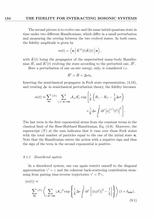
134 THE FIDELITY FOR INTERACTING BOSONIC SYSTEMS
The second picture is to evolve one and the same initial quantum state intime under two different Hamiltonians, which differ in a small perturbationand measuring the overlap between the two evolved states. In both cases,the fidelity amplitude is given by
m(t) =⟨n∣∣∣ K ′†(t)K(t)
∣∣∣n⟩ ,with K(t) being the propagator of the unperturbed many-body Hamilto-nian H, and K ′(t) evolving the state according to the perturbed one, H ′.
Here a perturbation of one on-site energy, only, is considered i.e.
H ′ = H + ∆εnl.
Inserting the semiclassical propagator in Fock state representation, (4.18),and treating ∆ε in semiclassical perturbation theory, the fidelity becomes
m(t) ≈∑m
(N)∑
γ,γ′:n→m
AγA∗γ′ exp
[i
h
(Rγ −Rγ′ −
1
2∆εt
)
+i
h∆ε
t∫0
dt′∣∣∣ψ(γ′)l (t′)
∣∣∣2 ].The last term in the first exponential stems from the constant terms in theclassical limit of the Bose-Hubbard Hamitlonian, Eq. (4.9). Moreover, thesuperscript (N) at the sum indicates that it runs over those Fock stateswith the total number of particles equal to the one of the initial state n.Note that the Hamiltonian enters the action with a negative sign and thusthe sign of the term in the second exponential is positive.
9.1.1 Disordered system
In a disordered system, one can again restrict oneself to the diagonalapproximation γ′ = γ and the coherent back-scattering contribution stem-ming from pairing time-reverse trajectories γ′ = T γ,
〈m(t)〉 ≈∑m
(N)
⟨ ∑γ:n→m
|Aγ |2 exp
i
h∆ε
t∫0
dt′[∣∣ψl(t′)∣∣2 − 1
2
]⟩
(1 + δnm) .
(9.1)

9.1. THE FIDELITY AMPLITUDE 135
Here, the term δnm originates again from the pairing of time reverse tra-jectories. When performing the disorder average, one can assume that theperturbation will not be always the same, but rather uniformly distributedwithin a certain range, which here will be chosen to be [ε/2,−ε/2].
Moreover, if the classical limit is chaotic the integral in the exponent in(9.1) can be interpreted as a sum over random variables. Hence, due to thecentral limit theorem it can be replaced by a gaussian distributed variableX. Then, the mean
〈X〉 =
⟨ t∫0
dt′[|ψl(t)|2 −
1
2
]⟩= n0t (9.2)
and the variance
⟨(X − 〈X〉)2
⟩=
⟨t∫
0
dt′[|ψl(t)|2 −
1
2
]2⟩− 〈X〉2 = σ2t (9.3)
are proportional to the time t. This behavior is expected due to the expo-nential decay of correlations in chaotic systems [265].
Furthermore, the mean can be easily estimated: thermalization [266–269] states that each site is on average equally occupied. The subtracted1/2 then cancels with the additional 1/2 introduced by the boundary condi-tions (4.19) and therefore the mean is given by the average particle densitymultiplied by the time,
〈X〉 = n0t =N
Lt.
Estimating σ2, however, is a much more difficult task and has not beenpossible up to now. However, one can expect that
σ2 =
⟨1
t
t∫0
dt′t−t′∫−t′
dτ∣∣ψl(t′)∣∣2 ∣∣ψl(t′ + τ)
∣∣2⟩− n0t− n20t−
t
4.
is independent on the time t.
Evaluating the integrals over X and ∆ε arising due to the averagingare then straightforward and yield
〈m(t)〉 ≈√
2π
t
h
εσexp
(− n2
0
2σ2t
)<Φ
(εσ2 + 2ihn0
2√
2hσ
√t
), (9.4)

136 THE FIDELITY FOR INTERACTING BOSONIC SYSTEMS
where
Φ(x) =2√π
x∫0
dz exp(−z2
)is the error function. Moreover, in (9.4), the result of the transition prob-ability has been used in order to replace
∑m
(N)
⟨ ∑γ:n→m
|Aγ |2⟩
(1 + δnm) = 1.
Using the asymptotic formula for the error function [270] then gives for thelarge time asymptotics, i.e. for t h√
ε2σ2+4h2n20/σ
2
〈m(t)〉 ≈ h
ε
[4h
t
2n0h sin(n0ε2h t)− εσ2 cos
(n0ε2h t)
ε2σ4 + 4n20h
2 exp
(−ε
2σ2
8h2 t
)
+
√2π
σ2texp
(− n2
0
2σ2t
)].
(9.5)
9.1.2 Short Time Behavior
On the other hand, as suggested by the results obtained in section 7.2,for short times the trajectory almost does not feel the disorder, but theparticles stay at their individual sites and only the phase evolves, such that
〈m(t)〉 ≈ 1
ε
ε2∫
− ε2
d∆ε exp
(i∆ε
hnlt
)=
2h sin(εnlt2h
)εnlt
, (9.6)
which yields when expanding up to second order in time the well knownquadratic initial decay [264]
〈m(t)〉 ≈ 1−(εnl
2h
)2 t2
6. (9.7)
The main observation here is that the decay becomes stronger when increas-ing the number of particles in the affected site. To the author’s knowledgethis is the first time that for a many-body system a prediction about thedependence of the fidelity on the number of particles has been made.

9.2. THE LOSCHMIDT ECHO 137
n
m
γ
γ∗′
γ∗γ′
Figure 9.2: Trajectory pairs giving rise to the background contribution.
9.2 The Loschmidt echo
Following [25], the average Loschmidt echo, which is the average of
the modulus of the fidelity, M(t) =⟨|m(t)|2
⟩can be written in the semi-
classical limit as a sum of two contributions. However, here due to thediscreteness of the basis, a third background contribution arises such that
M(t) ≈Minc(t) +Mcoh(t) +Mbg. (9.8)
In order to avoid confusion, the first term will be denoted as the incoherentand the second one as the coherent contribution. This notation will becomeclear in the following.
9.2.1 Background contribution
The Loschmidt echo M(t) in semiclassical perturbation theory is givenby
M(t) =∑m,m′
(N)
⟨ ∑γ,γ′:n→mγ∗,γ∗′:n→m′
AγA∗γ′A∗γ∗Aγ∗′ exp
i
h
(Rγ −Rγ′ −Rγ∗ +Rγ∗′
+∆ε
t∫0
dt′[∣∣∣ψ(γ′)
l
(t′)∣∣∣2 − ∣∣∣ψ(γ∗′)
l
(t′)∣∣∣2])⟩.
(9.9)

138 THE FIDELITY FOR INTERACTING BOSONIC SYSTEMS
Here, the trajectories with and without an asterisk originate from the timeevolution of m∗(t) and m(t), respectively. Moreover, a prime indicatesthat the trajectory corresponds to backward propagation. Here it becomesobvious that, apart from the usual (extended) diagonal pairing γ(∗)′ = γ(∗)
and γ(∗)′ = T γ(∗), one can also pair crosswise like in Fig. 9.2, i.e. γ∗′ =(T )γ′ and γ∗ = (T )γ in order to get vanishing action differences. However,this pairing requires that m′ = m. For a continuous basis, this would bea set of zero measure, and therefore these contributions did not arise infirst quantized approaches [25, 45, 46]. However, in this case the basis isdiscrete, and thus this contribution should be taken into account.
One immediately sees that for this kind of pairing also the contributionarising due to the perturbation to the phase cancels and therefore thebackground contribution is given by
Mbg(t) =∑m
(N)
⟨ ∑γ,γ′:n→m
|Aγ |2∣∣Aγ′∣∣2
⟩(1 + δnm)2
=∑m
(N)[P (cl) (m,n; t) (1 + δnm)
]2,
(9.10)
where in the second step the sum rule Eq. (7.2) has been used in order torelate the background contribution with the classical transition probabilityP (cl). Since the disorder averaged classical transition probability becomesconstant for large enough times t the background contribution can also beassumed to be time independent.
9.2.2 Incoherent contribution
Coming back to the usual pairing γ′ = γ or γ′ = T γ and γ(∗)′ =γ∗ or γ(∗)′ = T γ∗ (see Fig. 9.3), the incoherent contribution is given byconsidering those pairs of trajectories γ∗ and γ∗′ which generically are faraway in phase space from γ and γ′ and therefore explore different regionsin phase space. Therefore, the evolution of this part of m∗(t) is incoherentto the one of m(t) and hence the denotation as incoherent contribution.
Since the trajectories for m∗(t) and m(t) are far away from each other,the diagonal approximation as well as the averaging over the time integralof |ψl(t)|2 can be performed independently for m∗(t) and m(t). Followingthe above steps and again taking also into account the time reverse pairing,

9.2. THE LOSCHMIDT ECHO 139
n
m
m′
γγ∗
γ′
γ∗′
Figure 9.3: Trajectory pair determining the incoherent contribution.
this yields
Minc(t) =∑m,m′
(N)
⟨ ∑γ:n→mγ′:n→m′
∗ |Aγ |2∣∣Aγ′∣∣2
⟩(1 + δn,m)
(1 + δn,m′
)
×√π
t
h
εσΦ( εσ
2h
√t),
(9.11)
where the star at the double sum over trajectories indicates that only thosepairs are taken into account, which explore different regions in phase space.
By introducing
x =ε2σ2
4h2 t,
as well as
M(0)inc =
∑m,m′
(N)
⟨ ∑γ:n→mγ′:n→m′
∗ |Aγ |2∣∣Aγ′∣∣2
⟩(1 + δn,m)
(1 + δn,m′
),
Eq. (9.11) can be written in the compact form
Minc(t) = M(0)incF (x),
with
F (x) =1
2
√π
xΦ(√x). (9.12)

140 THE FIDELITY FOR INTERACTING BOSONIC SYSTEMS
0
0.2
0.4
0.6
0.8
1
0 5 10 15 20
F(x
)
x
Figure 9.4: Comparison of the function F (x), Eq. (9.12), (black) with itsasymptotics [
√π/x− exp(−x)/x]/2 (red) and
√π/x/2 (blue).
For large times, one can again use the asymptotic form of the error function[270], in order to get
F (x) ≈ 1
2
[√π
x− 1
xexp (−x)
]≈ 1
2
√π
x. (9.13)
In Fig. 9.4 both approximations are compared with the exact expressionfor F (x) showing that even the crude approximation F (x) ≈
√π/x/2 is
almost indistinguishable from the exact function F (x) already for x ≈ 4.
9.2.3 Coherent contribution
Computing the coherent contribution is somewhat more elaborate, sinceif all four trajectories are correlated (see Fig. 9.5) one can not perform theaverages over the time integrals in the second exponential in (9.9) inde-pendently. Instead, the difference should be computed by utilizing thelinearized equations of motion around e.g. γ′.
It should also be noted that both time integrals are invariant undertime-reversal. Thus in the following, it is enough to consider the pairingγ′ = γ and γ∗′ = γ∗ with γ∗ ∼ γ but γ∗ 6= γ. The contributions of timereverse pairing can then be easily incorporated at the end of the analysis.

9.2. THE LOSCHMIDT ECHO 141
n
m
m′
γ∗
γ
γ′ γ∗′
Figure 9.5: The coherent contribution is given by sets of four trajectories,which all stay close together during the whole time evolution.
The evolution determined by the linearized equations of motion are forlong enough times exponentially with the Lyapunov exponent λ. Since theinitial occupations of γ and γ∗ are the same, but the final one have to bem and m′, respectively, one finds [25]
t∫0
dt′[∣∣∣ψ(γ′)
l
(t′)∣∣∣2 − ∣∣∣ψ(γ∗)
l
(t′)∣∣∣2] ≈ (ml −m′l
) t∫0
dt′ exp[λ(t′ − t
)]=ml −m′l
λ[1− exp (−λt)] .
After integrating over ∆ε again, the coherent contribution reads
Mcoh(t) =∑m,m′
(N)
⟨ ∑γ:n→m
|Aγ |4⟩
(1 + δnm + δnm′)
×2λh sin
ε2λh [1− exp (−λt)] (ml −m′l)
ε [1− exp (−λt)]
(ml −m′l
) ,
(9.14)
where as usual the Kronecker deltas stem from pairing of time reversepaths.
For long enough times, the number of trajectories joining n with mtypically increases exponentially, while at the same time, |Aγ |2 decreasesexponentially with a rate given by the Lyapunov exponent. Thus,⟨ ∑
γ:n→m
|Aγ |4⟩∼ f(t) exp (−λt) , (9.15)
where f(t) is some algebraic function of time. Finally, for long times inEq. (9.14) one can approximate
1− exp (−λt) ≈ 1,

142 THE FIDELITY FOR INTERACTING BOSONIC SYSTEMS
such that
Mcoh(t) ∼ 2λh
εf(t) exp (−λt)
∑∆ml
sin(
ε2λh∆ml
)∆ml
,
where the sum now runs only over the differences between the final oc-cupations. Note that only differences up to a certain bound ∆ ± mmax,which is assumed to be ±1, should be taken into account in order to ensurethat all four trajectories stay close enough to each other, such that theircontribution survives the averaging.
9.3 Discussion and comparison with numericaldata
9.3.1 Fidelity
The fact that the fidelity is given by an Error function with a complexargument, immediately leads to oscillations in the fidelity similar to thoseobtained in a Bose-Hubbard trimer, i.e. a three-site Bose-Hubbard system,without disorder [271]. However, the average fidelity even has exact zeros,given by those times, at which the Error function in Eq. (9.4) gets purelyimaginary.
The semiclassical theory contains two parameters, which can be de-termined by fitting it to numerical data, namely the average occupationn0 of the l-th site and the variance σ introduced in Eq. (9.3). To thisend, the fidelity has been computed for a Bose-Hubbard ring consistingof five sites with nearest neighbor hopping strength J = 0.5, interactionstrength U = 4J and disorder strength W = 10J for a perturbationstrength ε = 0.04J . In these numerical calculations the initial state hasbeen chosen to be |2, 4, 3, 2, 3〉 having in total N = 14 particles and the av-erage runs over 24000 disorder realizations1. In addition, for every disorderrealization, the site which is perturbed is chosen randomly.
As discussed in section section 9.1.1, the average occupation can beexpected to be given approximately by the number of particles dividedby the number of single-particle states, which in the chosen case wouldbe n0 = 2.8. Actually the mean value in Eq. (9.2) has been computednumerically by Julien Dujardin in Liege predicting a value of n0 = 2.77.
1 Numerical data by courtesy of Peter Schlagheck

9.3. DISCUSSION 143
-0.2
0
0.2
0.4
0.6
0.8
1
0 100 200 300 400 500
Re[⟨
m(t
)⟩]
t [h/2J]
(a)
0.1
0.2
0.3
0.4
0.5
0.6
0.7
0.8
0.9
1
0 20 40 60 80 100
Re[⟨
m(t
)⟩]
t [h/2J]
(b)
Figure 9.6: (a) Comparison of the numerical data (black) for the real partof the fidelity amplitude with the fitted semiclassical prediction (red line)as well as the corresponding long time asymptotics (blue dotted line). (b)Comparison of the numerical data (black) for the real part of the fidelityamplitude with the fitted semiclassical prediction (red line) and the shorttime formula Eq. (9.6) (blue dashed line).
The values obtained from fitting the semiclassical theory to the numericaldata are
n0 ≈ 2.85, (9.16a)
σ ≈ 8.92, (9.16b)
where the value obtained for n0 is still in good agreement with the aboveestimate.
Fig. 9.6 shows that the semiclassical theory with the values given inEq. (9.16) agrees very well with the numerical data for ε = 0.04J .
It is worth to notice that both, the numerical data and the semiclassicaltheory, show the initial quadratic decay predicted by (9.7). Yet, in order toemphasize that the numerical data indeed initially has a quadratic behavior,Fig. 9.6(b) shows the numerical data in comparison with Eq. (9.6) for smalltimes. Again, the agreement of both curves is very good. Note, however,that since in the numerical study the site which has been perturbed hasbeen chosen randomly for each disorder realization, for a comparison onehas to replace nl by n0 in Eqns. (9.6,9.7).
It is obvious that the approximation Eq. (9.7) has to break down, beforethe first zero occurs. This is because this zero is related to the oscillations,which of course can not be covered by the quadratic approximation.

144 THE FIDELITY FOR INTERACTING BOSONIC SYSTEMS
-0.2
0
0.2
0.4
0.6
0.8
1
0 100 200 300 400 500
Re[⟨
m(t
)⟩]
t [h/2J]
(a)
0.9
0.91
0.92
0.93
0.94
0.95
0.96
0.97
0.98
0.99
1
0 20 40 60 80 100
Re[⟨
m(t
)⟩]
t [h/2J]
(b)
-0.4
-0.2
0
0.2
0.4
0.6
0.8
1
0 100 200 300 400 500
Re[⟨
m(t
)⟩]
t [h/2J]
(c)
0.65
0.7
0.75
0.8
0.85
0.9
0.95
1
0 20 40 60 80 100
Re[⟨
m(t
)⟩]
t [h/2J]
(d)
Figure 9.7: (a),(b) Comparison of the numerical data (black) for the realpart of the fidelity amplitude with the fitted semiclassical prediction (redline) for ε = 0.01J . (c),(d) Comparison of the numerical data (black) for thereal part of the fidelity amplitude with the fitted semiclassical prediction(red line) for ε = 0.02J and the short time formula, Eq. (9.6) (blue dashedline).
Moreover, Fig. 9.6(a) also compares the numerical results with the longtime behavior, Eq. (9.5). The cosine and sine in Eq. (9.5) indicate thatthe long time asymptotics may hold already before the fidelity becomeszero for the first time, since these terms are responsible for the oscillations.Indeed, the comparison in Fig. 9.6(a) holds good agreement already beforethe first zero occurs.
Finally, Fig. 9.7 shows a comparison of the semiclassical theory withthe numerical data for perturbation strengths ε = 0.01J and ε = 0.02J . Inthese figures for the semiclassical curves the parameters obtained from thefitting for ε = 0.04J have been used. However, in the numerical data, theaverage now runs over 200 disorder realizations only, which might explain

9.3. DISCUSSION 145
the stronger deviations compared to the plots shown in Fig. 9.6. Yet, theagreement between numerics and semiclassics is still very good.
As a matter of fact, Eq. (9.5) suggests that in principle, there mightbe two regimes, due to the decomposition into two terms, where each termdecreases exponentially, however with different rates. For small pertur-bations, the second exponential decreases much slower and therefore thiscontribution will dominate. Thus, for small perturbation, the exponentialdecrease is determined by the perturbation strength.
For larger perturbation strengths however, the first term may eventuallydominate and yield a decrease independent of the perturbation strength.Such a perturbation independent regime has been observed previously forthe Loschmidt echo [25], but not yet for the fidelity. However, the pertur-bation independent regime for the decay of the Loschmidt echo typicallydecreases with a decay rate given by the Lyapunov exponent [25] – and istherefore called Lyapunov regime –, whereas here the decay rate is deter-mined solely by the average occupation.
The perturbation strength, at which the first exponential starts to dom-inate can be estimated to be
εc ≈2n0h
σ2.
However, it remains the question, whether the above approach is still validin this regime, since the perturbation strength already has to be prettylarge, such that maybe the semiclassical perturbation theory is no longerjustified.
9.3.2 Loschmidt echo
The average Loschmidt echo also decreases quadratically for small times[272]. However, this quadratic decay can not be determined from the pre-sented semiclassical approach. After this initial quadratic decay, there is acompetition between the coherent and incoherent contribution, which de-termines its further decay. However, due to the asymptotic form, Eq. (9.13),the decay of the incoherent part Eq. (9.11) is algebraic, while the coherentpart, Eq. (9.14), decays exponentially. Thus, in the scenario consideredhere, the incoherent contribution will always win for large enough times.This also explains the absence of the Lyapunov regime in the numericalcalculations [272].

146 THE FIDELITY FOR INTERACTING BOSONIC SYSTEMS
Finally, for even larger times, when the coherent and incoherent con-tributions are negligibly small, the Loschmidt echo enters the saturationregime determined by the background contribution Eq. (9.10), which isindependent of time.
Assuming that in Eq. (9.15), f(t) ∼ tβ, the Loschmidt echo Eq. (9.8)can be written as
M(t) = tβ exp (−λt)∑∆ml
b∆ml
sinε∆ml2λh [1− exp (−λt)]
ε∆ml2λh [1− exp (−λt)]
+a
√π
t
h
εσΦ( εσ
2h
√t)
+ c,
(9.17)
where the fitting parameters
a = M(0)inc =
∑m,m′
(N)
⟨ ∑γ:n→mγ′:n→m′
∗ |Aγ |2∣∣Aγ′∣∣2
⟩(1 + δn,m)
(1 + δn,m′
),
b∆ml =exp (λt)
tβ
∑m
(N)
⟨ ∑γ:n→m
|Aγ |4⟩
(1 + δnm + δnm′) ,
c = Mbg =∑m
(N)
⟨ ∑γ,γ′:n→m
|Aγ |2∣∣Aγ′∣∣2
⟩(1 + δnm)2
have been introduced. Furthermore, σ, β and λ are obtained from fittingEq. (9.17) to the numerical data. It is expected, however, that b∆ml ≈ b isroughly the same number for all values of ∆ml smaller than or equal to anupper bound mmax for which the semiclassical perturbation theory remainsvalid and b∆ml = 0 for ∆ml > mmax.
While the variance σ has already been obtained from the fitting of thesemiclassical prediction of the amplitude in section 9.3.1 and is given byEq. (9.16b), the remaining parameters are obtained by two different fittingschemes.
Three-step fitting scheme
Here, it has been assumed that the maximum difference mmax in thefinal occupations for the coherent contribution has to be zero, in orderfor the semiclassical perturbation theory to be valid. Moreover, β hasbeen assumed to be zero. The remaining four fitting parameters are thenobtained in two steps: First, for very long time, due to its exponential

9.3. DISCUSSION 147
0.038
0.04
0.042
0.044
0.046
0.048
0.05
0.052
0.054
12000 14000 16000 18000 20000
⟨|m
(t)|
2⟩
t [h/2J]
Figure 9.8: Comparison of the numerical (black) and semiclassical (red line)calculation of the Loschmidt echo for very long times. For the semiclassicalcurve, the coherent contribution has been neglected.
behavior the coherent contribution can be assumed to be negligibly smallcompared to the remaining two. The coefficients of the remaining twocontributions are then obtained to be
a ≈ 0.577. (9.18a)
c ≈ 0.000189, (9.18b)
For long times, this step results in a very good agreement between thesemiclassical theory and numerical calculation as shown in Fig. 9.8. Theremaining two parameters b and λ are finally obtained from fitting thesemiclassical theory to the numerical data for intermediate times whileusing the parameters obtained in Eqns. (9.16) and (9.18) yielding
b ≈ 0.652, (9.19a)
λ ≈ 0.00105. (9.19b)
One-step fitting scheme
The second fitting scheme is to fit all parameters at once using as manynumerical points as possible. In this scenario mmax has been chosen to beone and β has also been kept as a fitting parameter. Moreover, b1 and b0
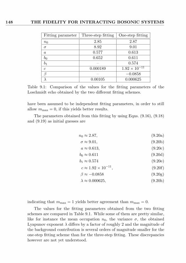
148 THE FIDELITY FOR INTERACTING BOSONIC SYSTEMS
Fitting parameter Three-step fitting One-step fitting
n0 2.85 2.87
σ 8.92 9.01
a 0.577 0.613
b0 0.652 0.611
b1 – 0.574
c 0.000189 1.92× 10⁻¹¹
β – −0.0858
λ 0.00105 0.000625
Table 9.1: Comparison of the values for the fitting parameters of theLoschmidt echo obtained by the two different fitting schemes.
have been assumed to be independent fitting parameters, in order to stillallow mmax = 0, if this yields better results.
The parameters obtained from this fitting by using Eqns. (9.16), (9.18)and (9.19) as initial guesses are
n0 ≈ 2.87, (9.20a)
σ ≈ 9.01, (9.20b)
a ≈ 0.613, (9.20c)
b0 ≈ 0.611 (9.20d)
b1 ≈ 0.574 (9.20e)
c ≈ 1.92× 10⁻¹¹, (9.20f)
β ≈ −0.0858 (9.20g)
λ ≈ 0.000625, (9.20h)
indicating that mmax = 1 yields better agreement than mmax = 0.
The values for the fitting parameters obtained from the two fittingschemes are compared in Table 9.1. While some of them are pretty similar,like for instance the mean occupation n0, the variance σ, the obtainedLyapunov exponent λ differs by a factor of roughly 2 and the magnitude ofthe background contribution is several orders of magnitude smaller for theone-step fitting scheme than for the three-step fitting. These discrepancieshowever are not yet understood.

9.3. DISCUSSION 149
Comparison with numerical results
Fig. 9.9 compares the thus obtained semiclassical predictions with thenumerical results and shows a very good overall agreement (see Fig. 9.9(a)).As expected, for very long times, both fitting schemes as well as the numer-ical result agree with the long time asymptotics obtained from neglectingthe coherent contribution. As can be easily seen in Fig. 9.9(c), for shortertimes, the latter of course can not reproduce the correct results. Insteadfor t . 2000h/J the three-step fitting scheme gives the best agreement,while later on the one-step fitting scheme does (see Fig. 9.9(d)).
The shoulder the one-step fitting result shows below t = 1000h/J sug-gest that the reason for this behavior is a crossover from mmax = 0 tommax = 1. This crossover can also be explained from a simple classicalargument: In the coherent contributions, the two trajectories are assumedto be close enough to each other in phase space to allow a linearization ofthe motion of one of the trajectories around the other one. Then, due toergodicity, the phase space distance between them increases exponentiallyin time. However, since the initial separation of the trajectories has to besmall enough, there is a certain minimal time required in order for the twotrajectories to end at different occupations. It is only after this minimaltime that the ∆ml = 1 term has to be included in the coherent contribu-tion. Including ∆ml = 2, on the other hand, seems not to be necessary,because at the time, at which the classical motion would allow for suchlarge deviations of the trajectories, the coherent contribution is alreadynegligible.
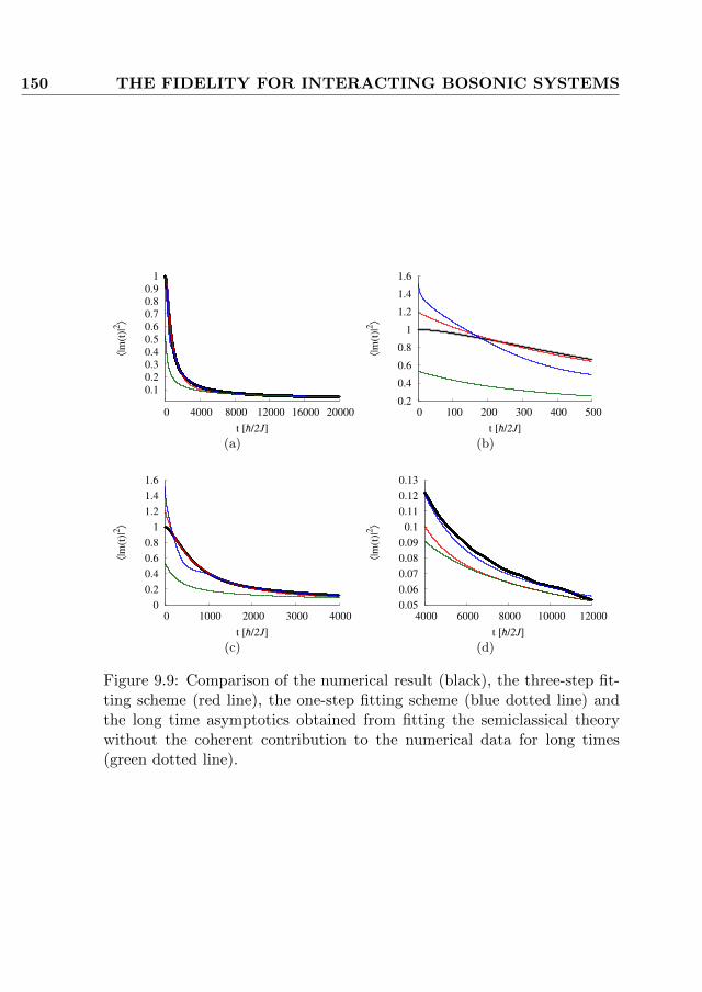
150 THE FIDELITY FOR INTERACTING BOSONIC SYSTEMS
0.1
0.2
0.3
0.4
0.5
0.6
0.7
0.8
0.9
1
0 4000 8000 12000 16000 20000
⟨|m
(t)|
2⟩
t [h/2J]
(a)
0.2
0.4
0.6
0.8
1
1.2
1.4
1.6
0 100 200 300 400 500
⟨|m
(t)|
2⟩
t [h/2J]
(b)
0
0.2
0.4
0.6
0.8
1
1.2
1.4
1.6
0 1000 2000 3000 4000
⟨|m
(t)|
2⟩
t [h/2J]
(c)
0.05
0.06
0.07
0.08
0.09
0.1
0.11
0.12
0.13
4000 6000 8000 10000 12000
⟨|m
(t)|
2⟩
t [h/2J]
(d)
Figure 9.9: Comparison of the numerical result (black), the three-step fit-ting scheme (red line), the one-step fitting scheme (blue dotted line) andthe long time asymptotics obtained from fitting the semiclassical theorywithout the coherent contribution to the numerical data for long times(green dotted line).
Part IV
Interference Effects inFermionic Fock Space
151


CHAPTER 10The Transition Probability
for Fermionic Systems
In section 7.1, it was shown that for a chaotic, bosonic many-body systemwhich is prepared in the Fock state n(i), the probability to measure attime tf the Fock state n(f) is enhanced by a factor of two compared to theclassical (Truncated Wigner) result if n(f) = n(i), while for all other n(f)
the classical and quantum probability coincide.
Now that a semiclassical propagator for fermionic systems has beenderived, one can ask, whether there is an analogous effect for fermions. Toaddress this question, consider a spin-1
2 system with some spin-coupling(e.g. Rashba spin-orbit interaction). Such a system may be for examplethe Fermi-Hubbard model with Rashba spin-orbit interaction α, describedby the Hamiltonian
H =
L∑l=1
[ ∑σ=↓,↑
(εlc†l,σ cl,σ − Jc
†l,σ cl+1,σ − J∗c†l+1,σ cl,σ
)+ Uc†l,↑c
†l,↓cl,↓cl,↑
+α(c†l,↓cl+1,↑ − c†l+1,↓cl,↑
)+ α∗
(c†l+1,↑cl,↓ − c
†l,↑cl+1,↓
) ].
(10.1)
Inserting the semiclassical propagator, (5.14), the transition probability isgiven by
153

154 THE TRANSITION PROBABILITY FOR FERMIONIC SYSTEMS
P(n(f),n(i); tf , ti
)=∣∣∣〈n(f)| K (tf , ti) |n(i)〉
∣∣∣2≈∑γ,γ′
AγBγA∗γ′Bγ′∗ exp
[i
h
(Rγ −Rγ′
)]
With the same arguments as in section 7.1, under disorder average, one canrestrict the double sum over trajectories by one sum over trajectories γ anda second one over partner trajectories γ′, which give rise to generic actiondifferences Rγ − Rγ′ , i.e. to action differences, which are independent onthe disorder realization.
10.1 Diagonal approximation
The most obvious partner causing a generic action difference is of courseagain γ′ = γ leading to the diagonal approximation. Obviously, the actionsof γ and γ′ as well as the prefactors Bγ and Bγ′ are equal. The sum rule(7.2) is valid for fermions, too, and therefore, the diagonal approximationto the transition probability for fermions is given by what will be calledthe classical transition probability,
P (cl)(n(f), tf ; n(i), ti
)=
2π∫0
dN−1θ(i)
(2π)N−1δN−1
[P(f)
0 n(n(i),θ(i); tf
)− P(f)
0 n(f)] ∣∣∣B (n(i),θ(i)
)∣∣∣2 .Here, n
(n(i),θ(i); t
)is the vector containing the modulus squares of the
time evolution of the initial state with the components
φ(i)l,σ =
√n
(i)l,σ exp
(iθ
(i)l,σ
).
Moreover, B(n(i),θ(i)
)is given by Bγ defined in Eq. (5.15) for the trajec-
tory γ with initial phases θ(i) and can be considered as a renormalizationof the classical probability due to vacuum fluctuations.

10.2. COHERENT BACKSCATTERING LIKE CONTRIBUTION 155
10.2 Coherent backscattering like contribution
For time reversal symmetric systems, a second possibility to chose thepartner trajectory γ′, is the time reversed trajectory of γ, i.e. γ′ = T γ.In the example stated in Eq. (10.1), time reversal is achieved, if J is real.However, here one has to be more careful with the time reversal operatoras for bosonic systems, because it depends on the choice of the couplingα. On the one hand, if α = 0, which corresponds to having two copies ofone and the same system of spinless fermions, the time reversal operatoris - just as in the bosonic case - identical to complex conjugation, and onecan follow section 7.1.2 to find that the transition probability is twice theclassical one, if n(f) = n(i), and equal to the classical one otherwise.
On the other hand in the presence of spin-orbit coupling, i.e. if α 6= 0,the time reversal operator is given by
T = −iσyC,
where σy is the (many-body) y-Pauli matrix acting on spin space, and Cis complex conjugation in site-|+z〉 , |−z〉 representation. Thus the timereverse of the trajectory γ is achieved by the replacement(
φl,↑ (ti + t)φl,↓ (ti + t)
)−→
(−φl,↓∗ (tf − t)φl,↑∗ (tf − t)
).
In particular this implies that the time reverse of the trajectory γ startsat Xn(f) and ends at Xn(i), where X is the matrix, which exchanges thespin-up and spin-down components, while its initial and final phases satisfy
θ(T γ,i)l,↑ = π − θ(γ,f)
l,↓
θ(T γ,i)l,↓ = −θ(γ,f)
l,↑
θ(T γ,f)l,↑ = π − θ(γ,i)
l,↓
θ(T γ,f)l,↓ = −θ(γ,i)
l,↑ .
(10.2)
Similar to the bosonic case, pairing the trajectory γ with its time reverseis only possible, if the final Fock state is the spin reversed of the initialone. Therefore, one has again to replace the trajectories γ by nearby ones,which connect spin reversed Fock states. However, here the trajectories γused to replace γ will be chosen somewhat differently than in the bosoniccase, namely to start at n(i) and end at Xn(f), because in this way theorigin of the final result is more transparent.

156 THE TRANSITION PROBABILITY FOR FERMIONIC SYSTEMS
Using the relations of the initial and final phases of the time reversedtrajectory with the ones of the original one, Eq. (10.2), leads to the actiondifference
Rγ −Rγ′ ≈ Rγ −RT γ + h(θ(γ,f) − θ(γ,i)
)·(n(f) −Xn(i)
).
Reminding oneself of the derivation of the semiclassical prefactors in section5.2.2, it is clear that Bγ is the same for γ and its time reverse T γ, just asthe second derivative of the action with respect to the initial and finaloccupation numbers is. Therefore
P (cbs)(n(f), tf ; n(i), ti
)=
δTRI
(2π)N−1
∑γ:n(i)→Xn(i)
|Bγ |2∣∣∣∣∣∣det
∂P(i)0 θ(γ,i)
∂(P
(f)0 Xn(i)
)∣∣∣∣∣∣ exp
[i
h(Rγ −RT γ)
]exp
[i(θ(γ,f) − θ(γ′,i)
)(n(f) −Xn(i)
)].
(10.3)
The next step is to determine the action difference Rγ − RT γ . Since theHamiltonian is the same for a trajectory and its time reverse, this actiondifference is determined by the kinetic parts only,
Rγ −RT γ = h
∫γ
dn · θ − h∫T γ
dn · θ
= h
∫γ
dn · θ − hL∑l=1
[ tf∫ti
dt [π − θl,↑(T − t)]∂
∂tnl,↑ (T − t)
+
tf∫ti
dt [−θl,↓(T − t)]∂
∂tnl,↓ (T − t)
]
= hπ
L∑l=1
(n
(f)l,↑ − n
(i)l,↑
),
(10.4)
where T = tf + ti. Finally, for n(f) = Xn(i), the action difference is givenby
Rγ −RT γ = πhL∑l=1
(n
(i)l,↓ − n
(i)l,↑
)= πhN − 2πhN (↑),

10.3. DISCUSSION 157
with N (i,↑) the initial total number of spin-up particles. We find then thatthe action difference is equal to hπ times an even (odd) number, if the totalnumber of particles is even (odd). Thus, under disorder average, after av-eraging over the final phases, the coherent backscattering-like contributionto the transition probability for spin-1
2 particles becomes
P (cbs)(n(f), tf ; n(i), ti
)=
(−1)NδTRIδn(f)↑ ,n
(i)↓δn
(f)↓ ,n
(i)↑P (cl)
(n(f), tf ; n(i), ti
),
and summing up the two leading order contributions yields
P(n(f), tf ; n(i), ti
)≈[
1 + (−1)NδTRIδn(f),Xn(i)
]P (cl)
(n(f), tf ; n(i), ti
).
(10.5)
All in all, the average transition probability can be written as
P(n(f), tf ; n(i), ti
)≈ P (cl)
(n(f), tf ; n(i), ti
)1 GUE
1 + δn(f)n(i) GOE
1 + (−1)Nδn(f),Xn(i) GSE,
where the notation of Random matrix symmetry classes [273] has beenimplied with GUE (gaussian unitary ensemble) denoting systems withouttime reversal invariance, GOE (gaussian orthogonal ensemble) time rever-sal symmetric systems without spin-orbit coupling and GSE (gaussian sym-plectic ensemble) those with both, time reversal symmetry and spin-orbitcoupling. This result and the pairing of trajectories for each symmetryclass is also summarized in Fig. 10.1.
10.3 Discussion
Eq. (10.5) says that the probability to measure a final Fock state whichis the spin reversed of the initial one is zero if the total number of particlesis odd, while it is twice the classical one if the total number of particlesis even. As already stated above, this holds only if the system is timereversal symmetric and there is a spin coupling mechanism which allowsthe transformation of spin-up to spin-down particles and no further discretesymmetries exist. Without spin coupling, the result would be given by
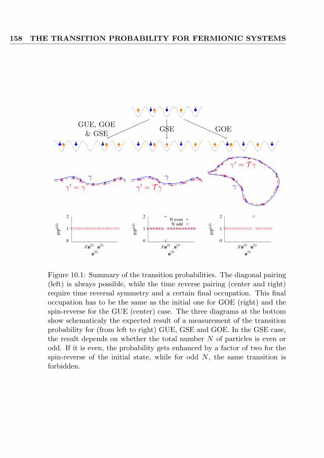
158 THE TRANSITION PROBABILITY FOR FERMIONIC SYSTEMS
γ
γ′ = T γγ
γ′ = T γγ
γ′ = γ
0
1
2
X n(i)
n(i)
P/P
(cl)
n(f)
0
1
2
X n(i)
n(i)
P/P
(cl)
n(f)
N evenN odd
0
1
2
X n(i)
n(i)
P/P
(cl)
n(f)
GUE, GOE& GSE
GSE GOE
Figure 10.1: Summary of the transition probabilities. The diagonal pairing(left) is always possible, while the time reverse pairing (center and right)require time reversal symmetry and a certain final occupation. This finaloccupation has to be the same as the initial one for GOE (right) and thespin-reverse for the GUE (center) case. The three diagrams at the bottomshow schematicaly the expected result of a measurement of the transitionprobability for (from left to right) GUE, GSE and GOE. In the GSE case,the result depends on whether the total number N of particles is even orodd. If it is even, the probability gets enhanced by a factor of two for thespin-reverse of the initial state, while for odd N , the same transition isforbidden.

10.4. FURTHER DISCRETE SYMMETRIES 159
(7.3). The fact that for n(f) = Xn(i), i.e. if the final Fock state is thespin-flipped version of the initial one, the averaged transition probability iszero and the transition probability itself is by construction a non-negativequantity, already implies that the transition probability is zero for everydisorder realization. In fact, it can be shown exactly for any quantumsystem with a time-reversal operator, which squares to minus one, T 2 = −1,that the transition probability between time reversed states is zero:
〈T φ| exp
(− i
hHt
)|φ〉 =
⟨T 2φ
∣∣∣∣ T exp
(− i
hHt
)φ
⟩∗= (−1)N
⟨φ
∣∣∣∣ exp
(i
hHt
)T φ⟩∗
= (−1)N 〈T φ| exp
(− i
hHt
)|φ〉 .
Therefore, for odd total number of particles
〈T φ| exp
(− i
hHt
)|φ〉 = 0.
which is a much easier and more general way to show that for an oddnumber of half-integer spin systems the transition from an initial state to itstime reverse (spin reverse) state vanishes. However, Eq. (10.5) on one handshows that the semiclassical technique introduced here can reproduce thedelicate phase coherences that produce even such an fundamental quantummechanical result, although the classical probability for this transition maybe non-zero. On the other hand, it is able to predict the result for an evennumber of particles, in which case the above argument tells nothing aboutthe transition probability.
10.4 Further discrete symmetries
If the spin-orbit coupling strength fulfills further conditions, additionaldiscrete symmetries may occur. For example, if α∗ = α, the system isinvariant under replacing all spin-up components by the negative of thespin-down ones and simultaneously replacing the spin-up by the spin-down
components. If initially n(i)l,↑ = n
(i)l,↓ for every site l, which is possible only for
an even total number of particles, there are two further possible partners foreach trajectory, while in all the other cases there is one additional possible
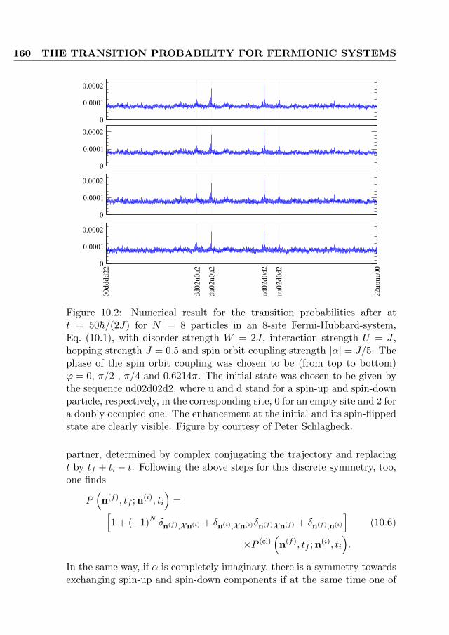
160 THE TRANSITION PROBABILITY FOR FERMIONIC SYSTEMS
0
0.0001
0.0002
0
0.0001
0.0002
0
0.0001
0.0002
00dddd22
dd02u0u2
du02u0u2
ud02d0d2
uu02d0d2
22uuuu00
0
0.0001
0.0002
Figure 10.2: Numerical result for the transition probabilities after att = 50h/(2J) for N = 8 particles in an 8-site Fermi-Hubbard-system,Eq. (10.1), with disorder strength W = 2J , interaction strength U = J ,hopping strength J = 0.5 and spin orbit coupling strength |α| = J/5. Thephase of the spin orbit coupling was chosen to be (from top to bottom)ϕ = 0, π/2 , π/4 and 0.6214π. The initial state was chosen to be given bythe sequence ud02d02d2, where u and d stand for a spin-up and spin-downparticle, respectively, in the corresponding site, 0 for an empty site and 2 fora doubly occupied one. The enhancement at the initial and its spin-flippedstate are clearly visible. Figure by courtesy of Peter Schlagheck.
partner, determined by complex conjugating the trajectory and replacingt by tf + ti − t. Following the above steps for this discrete symmetry, too,one finds
P(n(f), tf ; n(i), ti
)=[
1 + (−1)N δn(f),Xn(i) + δn(i),Xn(i)δn(f)Xn(f) + δn(f),n(i)
]×P (cl)
(n(f), tf ; n(i), ti
).
(10.6)
In the same way, if α is completely imaginary, there is a symmetry towardsexchanging spin-up and spin-down components if at the same time one of

10.4. FURTHER DISCRETE SYMMETRIES 161
0
0.0001
0.0002
0
0.0001
0.0002
0
0.0001
0.0002
00ddddd2
dd02u0uu
du02u0ud
ud02d0du
uu02d0dd
2uuuuu00
0
0.0001
0.0002
Figure 10.3: Numerical result for the transition probabilities at timet = 50h/(2J) for N = 7 particles in an 8-site Fermi-Hubbard-system,Eq. (10.1), with disorder strength W = 2J , interaction strength U = J ,hopping strength J = 0.5 and spin orbit coupling strength |α| = J/5. Thephase of the spin orbit coupling was chosen to be (from top to bottom)ϕ = 0, π/2 , π/4 and 0.6214π. The initial state was chosen to be given bythe sequence ud02d02d2, where u and d stand for a spin-up and spin-downparticle, respectively, in the corresponding site, 0 for an empty site and 2for a doubly occupied one. The enhancement at the initial state as wellas the vanishing probability for its spin-flipped version are clearly visible.Figure by courtesy of Peter Schlagheck.

162 THE TRANSITION PROBABILITY FOR FERMIONIC SYSTEMS
the two components gets multiplied by −1. This leads again to additionalpartner trajectories and finally to Eq. (10.6).
In fact, the result keeps the same for any phase ϕ of the couplingstrength α = |α| exp (iϕ) as long as it does not become site dependent.This is because the classical Hamiltonian is invariant under the transfor-mation (
ψ↑ψ↓
)→(ψ↓e
iϕ
ψ↑e−iϕ
).
As shown in Figs. 10.2 and 10.3, this prediction is nicely confirmed bynumerical calculations obtained by Peter Schlagheck.
In general, each discrete symmetry will give rise to further partner tra-jectories (and therefore further additive terms in the transition probability),which require certain conditions on the initial and final Fock state. In theaveraged transition probability, this condition will be reflected in a Kro-necker delta. Moreover, the phase of this contribution will be determinedby the difference in the kinetic parts of the actions. Since the result has tobe a real number, this phase will either be an integer multiple of π or eachsymmetry related partner will come in pairs such that each pair adds upto a real number.

CHAPTER 11Many-Body Spin Echo
11.1 The spin-echo setup
Since the prohibition of a transition from an initial Fock state to theone which is the spin reversed one for an odd number of spin-1
2 particles isno dynamical effect, and can be proven without any loss of generality byusing T 2 = −1, only the transition probability for fermions is a very nicecheck of the validity of the semiclassical approach presented here, but notmore.
On the other hand, there is a very famous effect in single-particle sys-tems based on constructive interference for spin-1
2 particles, namely thespin (or Hahn) echo [275], which is depicted in Fig. 11.1. In this spin-echoexperiment, spins are first of all aligned in z-direction along a constantmagnetic field (Fig. 11.1a). An intermediately applied radio frequencyfield then rotates the spins into x-direction (Fig. 11.1b), such that theystart to precess around the z-axes (Fig. 11.1c). After some time t, again aradio-frequency field is applied, in order to ratate the spins by 180 aroundthe y-axes (Fig. 11.1d). After letting the spins precess again for time t(Fig. 11.1e), all the spins point again into the same direction (Fig. 11.1f),independently on the different local magnetic field.
It is expected that due to relaxation processes and spin decoherence,the echo signal at time 2t, i.e. the enhancement of the probability of allspins pointing into the same direction shows a gaussian decay [276–279].Many-body effects have been included up to now only by means of spin-
163

164 MANY-BODY SPIN ECHO
Figure 11.1: Conventional spin echo experiment (cf. [274])
chains [280, 281], while spin-orbit interactions have not been considered atall.
Here, these last two points will be adressed. The focus of this sectionis on an interacting fermionic many-body system with spin-orbit coupling.However, in contrast to the conventional spin echo experiment [275], timereversal invariant systems will be considered. To this end, a system de-scribed for instance by the Hamiltonian Eq. (10.1) is considered, with theparameters chosen such that the classical limit Eq. (5.2) is chaotic.
It is furthermore assumed that the system is initially prepared in a Fockstate n(i), for which the single-particle states are ordered such that for eachorbital state the spin-down state follows the spin-up state,
|n〉 = |n1,↑, n1,↓, . . . , nL,↑, nL,↓〉 . (11.1)
This initial Fock state is then evolved for some time t1, after which, fora number F of the single-particle states, labeled by l1, . . . , lF , the spinsare reversed without measuring the number of particles within this state.Mathematically, this spin flip can be described by the operator
A =F∏j=1
[(1− nlj ,↑
)(1− nlj ,↓
)+ nlj ,↑nlj ,↓ + c†lj ,↑clj ,↓ + c†lj ,↓clj ,↑
]. (11.2)
In order to check that this linear operator indeed gives the correct spin-flip, one has to apply it to a Fock state |n〉. Thereby, the j-th factor in

11.1. THE SPIN-ECHO SETUP 165
K (t1)
A
K (t2)
Figure 11.2: Schematic sketch of the procedure of the spin-echo experiment
the product acts on the lj-th site only. The first term then is zero, if thelj-th site is occupied, and equal to the unity operator on this site if it isempty. In the same way, the second term is equal to unity, if the lj-thsite is fully, i.e. doubly, occupied, and zero else. Now, the last two termsare zero if the corresponding site is fully occupied or empty, while if itis singly occupied, the spin-up and spin-down component are exchanged.Therefore, the operator A indeed resembles the desired spin flip. However,one has to keep in mind that due to the antisymmetric nature of fermions,this operator will also yield an additional sign, which depends on the Fockstate, it is applied to and the choice of the ordering. Luckily, by the orderingchosen here, Eq. (11.1), these signs vanish.
The system is then let to evolve again for a time t2 and the resultingFock state is measured. For the example of spin-orbit coupled fermionicultra-cold atoms in an optical lattice this procedure is depicted in Fig. 11.2.However, the system does not need to be an ultra-cold atom system, butcan be any fermionic many-body system with spin-orbit interactions. Theonly requirements that will be made are the ergodicity of the classicalHamiltonian system and the invariance under the time reversal operator

166 MANY-BODY SPIN ECHO
T = −iσyC,
where σy is the Pauli matrix in y-direction and C denotes complex conju-gation.
11.2 Leading order contributions
The quantity analogous to the spin echo signal is the probability tomeasure a certain final Fock state n(f), which is given by
Pmbse
(n(f),n(i)
)=∣∣∣〈n(f)| K (t2) AK (t1) |n(i)〉
∣∣∣2 ,where K(t) is the propagator of the system. Inserting a unity operator interms of Fock states between A and K (t1) and inserting the semiclassicalapproximation for the propagator, Eq. (5.14), then yields a four-fold sumover trajectories,
Pmbse
(n(f),n(i)
)≈∑m,m′
∑γ1:n(i)→mγ2:Bm→n(f)
γ3:n(i)→m′
γ4:Bm′→n(f)
Aγ1Bγ1Aγ2Bγ2Aγ3∗Bγ3
∗Aγ4∗Bγ4
∗
× exp
[i
h(Rγ1 +Rγ2 −Rγ3 −Rγ4)
],
where B is the matrix, which exchanges the spin-up and spin-down com-ponents for those sites, for which the spin is flipped in between,
B =
b1. . .
bL
bl =
(
1 00 1
)if l /∈ l1, . . . , lF (
0 11 0
)if l ∈ (l1, . . . , lF )
Under disorder average, one has to find those combinations of trajectoriessuch that a trajectory contributing with a positive sign to the action differ-ence in the exponential is paired by one, which contributes with a negative

11.2. LEADING ORDER CONTRIBUTIONS 167
(a) (b)
Figure 11.3: Leading order contributions to the many-body spin-echo prob-ability.
sign. Neglecting all loop contributions, which have been introduced verybriefly in section 7.1.3 and are discussed in more detail in Appendix F, thisleaves in total eight possibilities for pairing. However, there are only twopossibilities, for which one of the sums over intermediate occupations mand m′ survives, and which therefore yield the leading order contribution.These two possibilities, which will be called incoherent and coherent con-tribution, are shown in Fig. 11.3. Note that the labeling as incoherent andcoherent contribution refers only to the many-body coherence, which is notincorporated in the classical limit.
The incoherent contribution, Fig. 11.3(a) is the diagonal approximationobtained by pairing γ1 = γ3 and γ2 = γ4, which is obviously only possible,if the intermediate occupations are equal, m′ = m, but does not requireany further conditions.
Using the definition of the classical transition probability in section 10.1,the diagonal approximation yields the classical or incoherent many-bodyspin-echo probability
P(incoh)mbse
(n(f),n(i); t1, t2
)=∑m
P (cl)(n(f),m; t2
)P (cl)
(m,n(i); t1
)= P
(cl)mbse
(n(f),n(i); t1, t2
),
which can be assumed to be approximately constant for all combinationsof n(f), n(i), t1 and t2, as long as the initial and final occupations are suchthat the particles are sufficiently distributed and t1 and t2 are large enoughthat the particles have been able to move.
The crosswise pairing shown in Fig. 11.3(b) of γ1 with the time reverseof γ4 as well as γ2 with the time reverse of γ3 is possible only if the twotimes t1 and t2 are comparable. Therefore the coherent contribution arisesonly for t1 ∼ t2. Moreover, it requires that the final Fock state is the timereverse version of the initial one, n(f) = Xn(i), where X is the matrix,
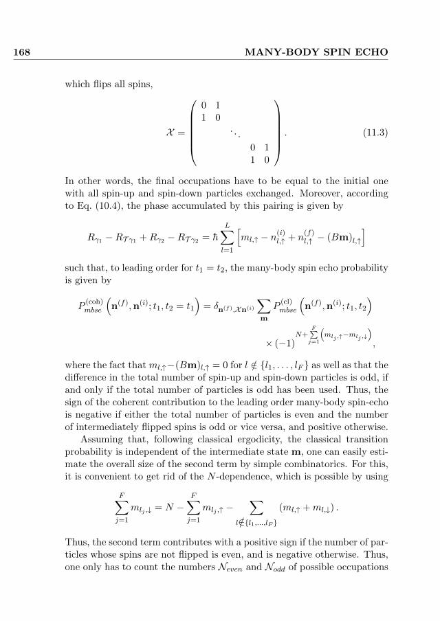
168 MANY-BODY SPIN ECHO
which flips all spins,
X =
0 11 0
. . .
0 11 0
. (11.3)
In other words, the final occupations have to be equal to the initial onewith all spin-up and spin-down particles exchanged. Moreover, accordingto Eq. (10.4), the phase accumulated by this pairing is given by
Rγ1 −RT γ1 +Rγ2 −RT γ2 = h
L∑l=1
[ml,↑ − n(i)
l,↑ + n(f)l,↑ − (Bm)l,↑
]such that, to leading order for t1 = t2, the many-body spin echo probabilityis given by
P(coh)mbse
(n(f),n(i); t1, t2 = t1
)= δn(f),Xn(i)
∑m
P(cl)mbse
(n(f),n(i); t1, t2
)
× (−1)N+
F∑j=1
(mlj ,↑−mlj ,↓
),
where the fact that ml,↑−(Bm)l,↑ = 0 for l /∈ l1, . . . , lF as well as that thedifference in the total number of spin-up and spin-down particles is odd, ifand only if the total number of particles is odd has been used. Thus, thesign of the coherent contribution to the leading order many-body spin-echois negative if either the total number of particles is even and the numberof intermediately flipped spins is odd or vice versa, and positive otherwise.
Assuming that, following classical ergodicity, the classical transitionprobability is independent of the intermediate state m, one can easily esti-mate the overall size of the second term by simple combinatorics. For this,it is convenient to get rid of the N -dependence, which is possible by using
F∑j=1
mlj ,↓ = N −F∑j=1
mlj ,↑ −∑
l/∈l1,...,lF (ml,↑ +ml,↓) .
Thus, the second term contributes with a positive sign if the number of par-ticles whose spins are not flipped is even, and is negative otherwise. Thus,one only has to count the numbers Neven and Nodd of possible occupations

11.2. LEADING ORDER CONTRIBUTIONS 169
m, for which the number of particles to which the spin-flip is not appliedif even and odd, respectively. These numbers are given by
Nodd =
dN2 e∑k=1
(2(L− F )
2k − 1
)(2F
N − 2k + 1
),
Neven =
bN2 c∑k=0
(2(L− F )
2k
)(2F
N − 2k
),
(11.4)
and thus give the coherent contribution for t1 = t2
P(coh)mbse
(n(f),n(i); t1, t2 = t1
)= δn(f),Xn(i)P
(cl)mbse
(n(f),n(i); t1, t1
)×(Neven −Nodd)
N
with N = Neven + Nodd being the number of occupations m with totalnumber of particles N .
What is left now is the time dependence of the coherent contribution tothe echo signal, i.e. the dependence on the echo time τ = t2−t1 if τ 6= 0. Inthis case the pairing of the trajectories requires to replace the trajectoriesγ2 and γ4 by trajectories, which evolve for time t1 instead of t2 and expandtheir actions in the exponential up to first order in τ . Using
∂Rγ(n(f),n(i); t
)∂t
= −Eγ ,
which can be proven using the equations of motion and the fact that thefinal occupations of both trajectories have to be the same, yields an addi-tional phase exp (i∆Eτ/h) for the coherent contribution, where ∆E is thedifference between the hopping terms in the energies of γ3 and γ1. Thisdifference solely stems from the different final phases of the two trajecto-ries, and therefore can be assumed to be on average uniformly distributedbetween ±E . For a chain with nearest neighbor-hopping, E is given thenby
E = 2κ
L−1∑l=1
∑σ=↑,↓
√nl,σnl+1,σ exp(−nl,σ − nl+1,σ),

170 MANY-BODY SPIN ECHO
where κ is the hopping parameter. This finally yields the leading ordermany-body spin-echo probability for small enough τ ,
Pmbse
(n(f),n(i); t1, t2 = t1 + τ
)=[
1 +(Neven −Nodd)
Nsin(Ehτ)
Ehτ
δn(f),Xn(i)
]P
(cl)mbse
(n(f),n(i); t1, t1
).
(11.5)
Thus as in the conventional spin echo, there is an echo signal, which isan change of the probability to measure a certain Fock state compared toall the others, if the second evolution time t2 is of the same order as thefirst one t1. The time width during which the probability is enhanced, canbe expected to be typically inverse proportional to the total number ofparticles through E .
With this result at hand, one can consider the special case that no spinsare flipped, i.e. F = 0. In this case, B becomes the 2L × 2L unit matrix,B = I2L, and it is easy to see that the many body spin echo probability,Eq. (11.5), recovers for τ = 0 the result for the transition probability forGSE, Eq. (10.5). For τ 6= 0, on the other hand, this is no longer true. Atfirst glance, this seems to be a contradiction to the result of Chapter 10,which yields for long enough times a time independent result. Thus, in theabsence of spin-flips, the coherent contribution should be treated somewhatdifferently, in order to obtain the semigroup property.
11.3 No spin-flips: Semigroup property
In order to recover the semigroup property, the crosswise pairing hasto be done in the way depicted in Fig. 11.4, i.e. by pairing γ1 = T γ4 andγ2 = T γ3. Note that in this case, the durations of the paired trajectoriesare in general not equal. Thus if t1 6= t2, the pairing γ1 = T γ4 should beunderstood as chosing the initial conditions of γ4 equal to the time reverseof the final conditions of γ1,
ψ(γ4)(0) = Xψ(γ1)∗(t1),
where X is given by Eq. (11.3). This initial condition ψ(γ4)(0) is thenclassically evolved up to time t2. The same construction holds for γ3. Notethat this procedure is not possible in the case with spin flips, since a spin

11.3. NO SPIN-FLIPS: SEMIGROUP PROPERTY 171
Figure 11.4: Coherent contribution to the many-body spin echo withoutspin flips.
flip would move the starting points of γ2 and γ4 away from the endingpoints of γ1 and γ3, respectively.
As can be seen from Fig. 11.4, this construction then requires thatthe trajectory γ2 is the continuation of γ1 and γ4 the continuation of γ3.In that way, this pairing coincides with the usual proof of the semigroupproperty for the semiclassical propagator by means of a stationary phaseapproximation [15, 282, 283], where the stationarity condition selects thosetrajectories, where the second is the continuation of the first one.
However, this in turn means that for instance if t1 > t2 the trajectoryγ1, which is fixed by the occupations n(i) and m, already determines m′ =
Xn(γ1)(t2), where n(γ)l (t) =
∣∣∣ψ(γ)l (t)
∣∣∣. The thus determined m′, on the
other hand, does not have to have integer entries. Therefore in order topair in the discussed way, γ3 and γ4 will have to be replaced by nearbytrajectories with final and initial occupations given by Xn(γ1)(t2). Duringthis replacement, the action in the phase of the propagator would haveto be expanded up to first order in the difference m′ − Xn(γ1)(t2), whichhowever cancels, since ψ(γ4)(0) = ψ(γ3)(t2).
Finally, this kind of pairing requires that the initial occupation is thetime reverse version of the final one, n(f) = Xn(i), such that followingsection 10.2, the contribution of the crosswise time-reverse pairing is givenby
P (coh)(n(f),n(i); t1, t2
)=
(−1)N∑m
P (cl)(n(f),m; t2
)P (cl)
(m,n(i); t1
)δn(f),Xn(i) ,
such that to leading order the transition probability, Eq. (10.5), is ob-tained, yielding the validity of the semigroup property of the semiclassicalpropagator in fermionic Fock sapce.

172 MANY-BODY SPIN ECHO
1
2
0
Pmbse/P
mbse
(incoh)
τ
τN
1
2
0 1 2 3 4 5 6
F
N=6
(a)
0
1
2
0 1 2 3 4 5 6
F
N=7
(b)
0
1
2
0 1 2 3 4 5 6
F
N=9
(c)
1
2
0 1 2 3 4 5 6
F
N=10
(d)
Figure 11.5: Time dependence of the the many-body spin echo for thecase of flipping all spins and n(f) = Xn(i). Insets: Size of the coherentcontribution at t2 = t1 for a six single-particle states with (a) six, (b)seven, (c) nine and (d) ten particles. as a function of the number F ofsingle-particle states, for which the spins are flipped.
11.4 Discussion of the results
With the peace of mind we get since the result Eq. (11.5) does not con-tradict with the calculations of the transition probability, one can continueto discuss the results. To this end, let’s start with the second obvious caseof F = L, in which all the spins are flipped, such that also B = X . Then,obviously, the coherent contribution has a positive sign for every interme-diate occupation m no matter whether the total number of particles is evenor odd, and the probability to measure at time 2t1 the spin-reverse of theinitial Fock state is twice the classical one,
Pmbse
(n(f),n(i); t1, t2 = t1 + τ
)=[
1 +sin(Ehτ)
Ehτ
δn(f),Tn(i)
]P
(incoh)mbse
(n(f),n(i); t1, t1
).
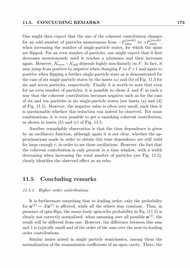
11.5. CONCLUDING REMARKS 173
One might then expect that the size of the coherent contribution changes
for an odd number of particles monotonous from −P (incoh)mbse to +P
(incoh)mbse ,
when increasing the number of single-particle states, for which the spinsare flipped. For an even number of particles, one might expect that it firstdecreases monotonously until it reaches a minimum and then increasesagain. However, Neven−Nodd depends highly non-linearly on F . In fact, itmay jump from positive to negative when changing F to F +1 and again topositive when flipping a further single-particle state as is demonstrated forthe case of six single-particle states by the insets (a) and (b) of Fig. 11.5 forsix and seven particles, respectively. Finally it is worth to note that evenfor an even number of particles, it is possible to chose L and F in such away that the coherent contribution becomes negative such as for the caseof six and ten particles in six single-particle states (see insets (a) and (d)of Fig. 11.5). However, the negative value is often very small, such that itis questionable whether this reduction can indeed be observed. For somecombinations, it is even possible to get a vanishing coherent contribution,as shown in insets (b) and (c) of Fig. 11.5.
Another remarkable observation is that the time dependence is givenby an oscillatory function, although again it is not clear, whether the ap-proximations made in order to obtain this time dependence are still validfor large enough τ , in order to see these oscillations. However, the fact thatthe coherent contribution is only present in a time window, with a widthdecreasing when increasing the total number of particles (see Fig. 11.5),clearly identifies the observed effect as an echo.
11.5 Concluding remarks
11.5.1 Higher order contributions
It is furthermore surprising that to leading order, only the probabilityfor n(f) = Xn(i) is affected, while all the others stay constant. Thus, inpresence of spin-flips, the many-body spin-echo probability in Eq. (11.5) isclearly not correctly normalized: when summing over all possible n(f), theresult will be different from one. However, the difference between this sumand 1 is typically small and of the order of the sum over the next-to-leadingorder contributions.
Similar issues arised in single particle semiclassics, among them thenormalization of the transmission coefficients of an open cavity. There, the

174 MANY-BODY SPIN ECHO
(a) (b)
(c) (d)
(e) (f)
(g) (h)
Figure 11.6: Next-to-leading order contributions to the many-body spin-echo probability
loop contributions have been found to solve this problem [21].These next-to-leading order contributions stem from the six remain-
ing diagrams, where ever two trajectories are the same or time reverse ofeach other (see Figs. 11.6(a)-(f)), as well as the two diagrams with a two-encounter, for which the sum over the intermediate occupations survives,Figs. 11.6(g),(h).
Concerning the loop contributions, i.e. the latter two, it should be notedthat one-leg- and no-leg-loops (see Appendix F) do not arise here, since –after replacing γ2 and γ4 by nearby trajectories with propagation time t1

11.5. CONCLUDING REMARKS 175
– all four trajectories are evolved for the same time, which in turn requiresthat if one trajectory starts or ends during traversing the encounter theremaining three also do. However, this case is already included in theremaining eight diagrams, Figs. 11.3,11.6(a)-(f).
The contributions from the diagonal like diagrams can be easily calcu-lated in the same way as the incoherent and coherent contribution above,while the computation of the loop contributions needs a little bit more care,since now there are two sources of action difference, which are the pairingof time reverse links on the one hand, and the encounter itself on the other.Consider for example diagram 11.6(g), where γ2 follows the time reverse ofγ3 and γ4 the time reverse of γ1 from the initial until the time, where theyenter the encounter, which shall be denoted as t0. The action differencestemming from these two links is according to Eq. (10.4) given by
πhL∑l=1
[∣∣∣ψ(γ2)l,↑ (t0)
∣∣∣2 − (Bm)l,↑ −∣∣∣ψ(T γ1)l,↑ (t0)
∣∣∣2 +(Bm′
)l,↑
].
The differences between γ4 and γ2 within the encounter, however are small,such that one can neglect the difference in their occupations, when enteringthe encounter, ∣∣∣ψ(γ2)
l,↑ (t0)∣∣∣2 − ∣∣∣ψ(T γ1)
l,↑ (t0)∣∣∣2 ≈ 0.
Furthermore using the condition on the intermediate occupations requiredby this diagram, XBm′ = m, the action difference originating from thelinks is given by
πh
L∑l=1
[(Xm)l,↑ − (Bm)l,↑
].
In order to evaluate the contribution of the encounter, one has to keep inmind that, as discussed above, on the one hand all four links need to havepositive duration, and on the other hand, if one link vanishes, the secondvanishes, too. Thus the density of phase space separations, Eq. (F.12), herehas to be replaced by
w (s,u) =t1 − tencΩN tenc

176 MANY-BODY SPIN ECHO
which yields for the contribution of Fig. 11.6(g)
P(g)mbse
(n(f),n(i); t1, t2
)=
∑m
(−1)
L∑l=1
[(X−B)m]l,↑P (cl)
(n(f), Bm; t2
)P (cl)
(m,n(i); t1
)
×c∫−c
d2L−2u
c∫−c
d2L−2st1 − tencΩN tenc
exp (iNs · u).
The integral over the stable and unstable components can then be per-formed following section 7.1.3, and the contribution of Fig. 11.6(h) can becalculated similarly.

11.5. CONCLUDING REMARKS 177
The next-to-leading order contributions are therefore found to read
P(a)mbse
(n(f),n(i); t1, t2
)=P (cl)
(n(f), BXn(i); t2
)P (cl)
(Xn(i),n(i); t1
)× (−1)N
P(b)mbse
(n(f),n(i); t1, t2
)=P (cl)
(n(f),Xn(f); t2
)P (cl)
(BXn(f),n(i); t1
)× (−1)N
P(c)mbse
(n(f),n(i); t1, t2
)=P (cl)
(n(f),Xn(f); t2
)P (cl)
(Tn(i),n(i); t1
)×δn(f),Bn(i)
P(d)mbse
(n(f),n(i); t1, t2
)=P (cl)
(n(f),n(i); t2
)P (cl)
(n(f),n(i); t1
)×sin
(Ehτ)
Ehτ
δn(f),Bn(i)
P(e)mbse
(n(f),n(i); t1, t2
)=P (cl)
(n(f),n(i); t2
)P (cl)
(Bn(i),n(i); t1
)× (−1)
L∑l=1
[(B−I2L)n(i)]l,↑ sin
(Ehτ)
Ehτ
δn(f),Xn(i)
P(f)mbse
(n(f),n(i); t1, t2
)=P (cl)
(n(f), Bn(f); t2
)P (cl)
(n(f),n(i); t1
)× (−1)
L∑l=1
[(I2L−B)n(f)]l,↑ sin
(Ehτ)
Ehτ
δn(f),Xn(i)
P(g)mbse
(n(f),n(i); t1, t2
)=−
∑m
P (cl)(n(f), Bm; t2
)P (cl)
(m,n(i); t1
)
× (−1)
L∑l=1
[(X−B)m]l,↑(
2π
N
)2L−2 1
2ΩN
sin(Ehτ)
Ehτ
P(h)mbse
(n(f),n(i); t1, t2
)=−
(2π
N
)2L−2 (−1)N
2ΩNP
(cl)mbse
(n(f),n(i); t1, t2
)×δn(f),Xn(i)
One can expect that ∑m
(N)(2π
N
)2L−2 1
2ΩN= O(1),
which a posteriori justifies, the consideration of the diagrams 11.6(g),(h),in the next-to leading order. When considering the normalization of the

178 MANY-BODY SPIN ECHO
many-body spin-echo probability, this assumption becomes even more ev-ident by noticing that when summing over the final occupations, only thediagrams 11.6(a),(b) and (g) can be of next-to-leading order and there-fore of the same order as the coherent contribution. Futhermore, fromthese three contributions only the last one has the same time-dependenceas the coherent contribution, and can therefore cancel it. The remaining
two contributions P((a))mbse and P
((b))mbse then restore the original value of the
normalization up to next-to-leading order.
11.5.2 Incomplete spin flips
Since the occupations should not be measured when applying the spinflip, it may be that it is incomplete, i.e. that the spins are not completelyflipped but brought into a superposition of up and down, such that themeasured object is given by
P ′mbse
(n(f),n(i); t2, t1
)=∣∣∣〈n(f)| K (t2)
(α+ βA
)K (t1) |n(i)〉
∣∣∣2= |α|2 P
(n(f),n(i); t1 + t2
)+ |β|2 Pmbse
(n(f),n(i); t1, t2
)+ 2<αβ∗
⟨n(f)
∣∣∣ K (t2 + t1)∣∣∣n(i)
⟩⟨n(f)
∣∣∣ K (t2) AK (t1)∣∣∣n(i)
⟩∗,
with 0 ≤ |α| , |β| ≤ 1 as well as |α+ β|2 = 1. Here, P (n(f),n(i); t2 + t1) isthe transition probability from n(i) to n(f) when evolving the system fortime t1 +t2 according to Chapter 10, and Pmbse is the many-body spin-echoprobability computed before in Eq. (11.5). Thus, one only has to determinethe last term which after inserting the semiclassical approximation for thepropagator, Eq. (5.14), is given by a sum over three trajectories,⟨
n(f)∣∣∣ K (t2 + t1)
∣∣∣n(i)⟩⟨
n(f)∣∣∣ K (t2) AK (t1)
∣∣∣n(i)⟩∗
=∑m
∑γ0:n(i)→n(f)
∑γ1:n(i)→mγ2:Bm→n(f)
Aγ0A∗γ1A∗γ2Bγ0B∗γ1
B∗γ2
× exp
[i
h(Rγ0 −Rγ1 −Rγ2)
].
Here, γ0 is propagated for time t1 + t2, while γ1 is evolved for time t1 andγ2 for time t2 only. Thus, pairing in such a way that all three trajectories
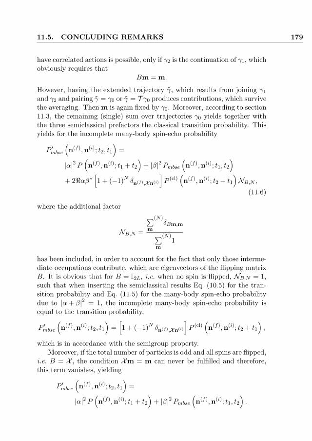
11.5. CONCLUDING REMARKS 179
have correlated actions is possible, only if γ2 is the continuation of γ1, whichobviously requires that
Bm = m.
However, having the extended trajectory γ, which results from joining γ1
and γ2 and pairing γ = γ0 or γ = T γ0 produces contributions, which survivethe averaging. Then m is again fixed by γ0. Moreover, according to section11.3, the remaining (single) sum over trajectories γ0 yields together withthe three semiclassical prefactors the classical transition probability. Thisyields for the incomplete many-body spin-echo probability
P ′mbse
(n(f),n(i); t2, t1
)=
|α|2 P(n(f),n(i); t1 + t2
)+ |β|2 Pmbse
(n(f),n(i); t1, t2
)+ 2<αβ∗
[1 + (−1)N δn(f),Xn(i)
]P (cl)
(n(f),n(i); t2 + t1
)NB,N ,
(11.6)
where the additional factor
NB,N =
∑m
(N)δBm,m∑
m
(N)1
has been included, in order to account for the fact that only those interme-diate occupations contribute, which are eigenvectors of the flipping matrixB. It is obvious that for B = I2L, i.e. when no spin is flipped, NB,N = 1,such that when inserting the semiclassical results Eq. (10.5) for the tran-sition probability and Eq. (11.5) for the many-body spin-echo probabilitydue to |α+ β|2 = 1, the incomplete many-body spin-echo probability isequal to the transition probability,
P ′mbse
(n(f),n(i); t2, t1
)=[1 + (−1)N δn(f),Xn(i)
]P (cl)
(n(f),n(i); t2 + t1
),
which is in accordance with the semigroup property.Moreover, if the total number of particles is odd and all spins are flipped,
i.e. B = X , the condition Xm = m can never be fulfilled and therefore,this term vanishes, yielding
P ′mbse
(n(f),n(i); t2, t1
)=
|α|2 P(n(f),n(i); t1 + t2
)+ |β|2 Pmbse
(n(f),n(i); t1, t2
).

180 MANY-BODY SPIN ECHO
Assuming that∑m
P (cl)(n(f), Bm; t2
)P (cl)
(m,n(i)
)≈ P (cl)
(n(f),n(i); t2 + t1
),
for equal propagation times before and after the spin flip, this probabilitycan be written to leading order as
P ′mbse
(n(f),n(i); t2, t1
)=
P (cl)(n(f),n(i); t1 + t2
) [|α|2 + |β|2 + δn(f),Xn(i)
(|β|2 − |α|2
)]Thus, for the case of flipping all spins and an odd number of particles,the incomplete many-body spin-echo probability interpolates between thecases β = 0 and β = 1. Interestingly, for |α| = |β|, the resulting probabilityis equal to the classical one, and therefore all interference effects vanish toleading order.

CHAPTER 12Many-Body Spin Fidelity
Reverting all the spins in a many-body system with spin-orbit coupling isalmost the time reversal operation. The fact that it is not exactly timereversal resembles itself in the non-vanishing probability to get n(f) 6= n(i)
in the many-body spin echo introduced in Chapter 11.
In analogy to this spin echo, this chapter deals with what will be calledthe many-body spin fidelity, which differs from the spin echo by propagatingthe system backwards in time after applying the spin flip, i.e. the observableof interest here is the spin-fidelity defined as
MF (t) =∣∣∣〈n(f)| K† (t) AK (t) |n(i)〉
∣∣∣2 ,with A given by (11.2). Since the evaluation of the spin fidelity is prettysimilar to the one of the spin echo, it will be kept somewhat shorter here.
After inserting the semiclassical propagator (5.14), the spin-fidelity be-comes a four fold sum over classical trajectories,
MF (t) ≈ (12.1)
Again, when performing a disorder average for large total number of parti-cles, the actions in the exponential give rise to large oscillations which willcancel on average, as long as the trajectories are not pairwise correlated.Those trajectory pairs, which exhibit at most one 2-encounter are shownin Figs. 12.1 and 12.2. Their contributions to the spin-fidelity are shownin Table 12.1 and 12.2.
181

182 MANY-BODY SPIN FIDELITY
(a) (b)
(c) (d)
(e) (f)
(g) (h)
(i) (j)
(k) (l)
Figure 12.1: First part of diagrams contributing to the spin fidelity,Eq. (12.1), with at most one 2-encounter.

MANY-BODY SPIN FIDELITY 183
(m) (n)
(o) (p)
(q) (r)
(s) (t)
(u) (v)
(w) (x)
Figure 12.2: Second part of diagrams contributing to the spin fidelity,Eq. (12.1), with at most one 2-encounter.
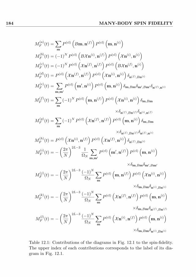
184 MANY-BODY SPIN FIDELITY
M(a)F (t) =
∑m
P (cl)(Bm,n(f)
)P (cl)
(m,n(i)
)M
(b)F (t) = (−1)N P (cl)
(BXn(i),n(f)
)P (cl)
(Xn(i),n(i)
)M
(c)F (t) = (−1)N P (cl)
(Xn(f),n(f)
)P (cl)
(BXn(f),n(i)
)M
(d)F (t) = P (cl)
(Xn(f),n(f)
)P (cl)
(Xn(i),n(i)
)δn(f),Bn(i)
M(e)F (t) =
∑m,m′
P (cl)(m′,n(i)
)P (cl)
(m,n(i)
)δm,Bmδm′,Bm′δn(f),n(i)
M(f)F (t) =
∑m
(−1)N P (cl)(m,n(f)
)P (cl)
(Xn(i),n(i)
)δm,Bm
×δn(f),Bn(f)δn(i),n(f)
M(g)F (t) =
∑m
(−1)N P (cl)(Xn(f),n(f)
)P (cl)
(m,n(i)
)δm,Bm
×δn(f),Bn(f)δn(f),n(i)
M(h)F (t) = P (cl)
(Xn(i),n(f)
)P (cl)
(Xn(f),n(i)
)δn(f),Bn(i)
M(i)F (t) = −
(2π
N
)2L−3 1
ΩN
∑m,m′
P (cl)(m′,n(f)
)P (cl)
(m,n(i)
)×δm,Bmδm′,Bm′
M(j)F (t) = −
(2π
N
)2L−3 (−1)N
ΩN
∑m
P (cl)(m,n(f)
)P (cl)
(Xn(i),n(i)
)×δm,Bmδn(i),Bn(i)
M(k)F (t) = −
(2π
N
)2L−3 (−1)N
ΩN
∑m
P (cl)(Xn(f),n(f)
)P (cl)
(m,n(i)
)×δm,Bmδn(f),Bn(f)
M(l)F (t) = −
(2π
N
)2L−3 (−1)N
ΩN
∑m
P (cl)(Xn(i),n(f)
)P (cl)
(m,n(i)
)×δm,Bmδn(i),Bn(i)
Table 12.1: Contributions of the diagrams in Fig. 12.1 to the spin-fidelity.The upper index of each contributions corresponds to the label of its dia-gram in Fig. 12.1.

MANY-BODY SPIN FIDELITY 185
M(m)F (t) = −
(2π
N
)2L−3 (−1)N
ΩN
∑m
P (cl)(m,n(f)
)P (cl)
(Xn(f),n(i)
)×δm,Bmδn(f),Bn(f)
M(n)F (t) = −
(2π
N
)2L−3 1
ΩNP (cl)
(Xn(i),n(f)
)P (cl)
(Xn(f),n(i)
)×δn(i),Bn(i)δn(f),Bn(f)
M(o)F (t) = −
(2π
N
)2L−3 (−1)N
ΩNP (cl)
(BXn(f),n(f)
)P (cl)
(Xn(f),n(i)
)M
(p)F (t) = −
(2π
N
)2L−3 (−1)N
ΩN
∑m
P (cl)(Xn(f),n(f)
)P (cl)
(m,n(i)
)×δn(f),n(i)δn(f),Bn(f)δm,Bm
M(q)F (t) = −
(2π
N
)2L−3 1
ΩN
∑m
P (cl)(Bm,n(f)
)P (cl)
(m,n(i)
)δn(f),n(i)
M(r)F (t) = −
(2π
N
)2L−3 (−1)N
ΩNP (cl)
(XBn(i),n(f)
)P (cl)
(Xn(i),n(i)
)×δn(f),n(i)
M(s)F (t) = −
(2π
N
)2L−3 (−1)N
ΩNP (cl)
(Xn(i),n(f)
)P (cl)
(XBn(i),n(i)
)×δn(f),n(i)
Table 12.2: Contributions of the diagrams in Fig. 12.2 to the spin-fidelity.The upper index of each contributions corresponds to the label of its dia-gram in Fig. 12.2.

186 MANY-BODY SPIN FIDELITY
M(t)F (t) = −
(2π
N
)2L−3 (−1)N
ΩNP (cl)
(Xn(f),n(f)
)P (cl)
(XBn(i),n(i)
)×δn(i),n(f)
M(u)F (t) = −
(2π
N
)2L−3 (−1)N
ΩNP (cl)
(XBn(i),n(f)
)P (cl)
(Xn(i),n(i)
)×δn(f),n(i)
M(v)F (t) = −
(2π
N
)2L−3 1
ΩNP (cl)
(Xn(f),n(f)
)P (cl)
(Xn(i),n(i)
)×δn(i),Bn(i)δn(f),Bn(f)
M(w)F (t) = −
(2π
N
)2L−3 (−1)N
ΩN
∑m
P (cl)(m,n(f)
)P (cl)
(Xn(i),n(i)
)×δm,Bmδn(i),n(f)δn(f),Bn(f)
M(x)F (t) = −
(2π
N
)2L−3 (−1)N
ΩNP (cl)
(Xn(i),n(f)
)P (cl)
(XBn(i),n(i)
)Table 12.3: Contributions of the diagrams in Fig. 12.2 to the spin-fidelity.The upper index of each contributions corresponds to the label of its dia-gram in Fig. 12.2.
The order of each diagram can be determined by the number of sumsover the intermediate occupations, which survive the averaging. However,
although a proof of this is missing, it is assumed that(N2π
)2L−3ΩN , where
ΩN =
∫d4Lψδ (θ1,↑) δ
N − L∑l=1
∑σ=↑,↓
|ψl,σ|2 .
is the phase space volume for fixed total number N of particles, is of thesame order as the sum over occupations,(
N
2π
)2L−3
ΩN ∼∑m
δ∑l,σ
ml,σ ,N. (12.2)
Thus, diagram 12.1(q) is for instance of the same order of magnitude as di-agram 12.1(d). Restricting oneself to leading and next to leading order, the

12.1. UNITARITY 187
many-body spin-fidelity is given by diagrams 12.1(a), (e)-(g) and 12.1(i),
MF (t) ≈∑m
P (cl)2
1 + δm,Bm
[2 (−1)N δn(f),Bn(f)δn(f),n(i)
+∑m′
δm′,Bm′
(δn(f),n(i) −
(2π
N
)2L−3 1
ΩN
)].
(12.3)
At this point it should be noted that only those encounter diagrams involv-ing all four trajectories are taken into account since those which involve onlytwo trajectories have been shown to cancel in section 7.1.3. Moreover, inthe situation considered here, there are no one-leg-loops formed by all fourtrajectories, since the fact that the propagation times are the same requiresthat if one link vanishes a second one also has to vanish thus forming againone of the diagrams in Fig. 12.1.
12.1 Unitarity
Before discussing the result, Eq. (12.3), in more detail consider the caseof no spin flips, i.e. A = 1, which also implies B = I2L. In this case,due to unitarity of the propagator, the spin-fidelity obviously should beMF (t) = δn(i),n(f) . Comparing Eq. (12.3) with this expectation furtheraffirms the assumption Eq. (12.2), which leads to a cancellation of the firstand the last term for F = 0 and therefore leads to a result proportional to aKronecker delta in the initial and final occupations. Therefore, encounterdiagrams have indeed to be taken into account and can be of the sameorder of magnitude as diagrams without encounter.
Consider now the next-to-next-to-leading order diagrams. In order toshow the unitarity within this order, one has to recognize that the diagrams12.1(j) and (l) ((k) and (m)) are of the same order as Fig. 12.1(b) ((c)).However, since the sum over trajectories γ1 (γ4) for the diagonal terms in-clude both, γ1 (γ4) and T γ1 (T γ4), there are twice as many contributionscorresponding to the diagram 12.1(b) (12.1(c)) than those corresponding tothe diagrams 12.1(j) and (l) (Figure 12.1(k) and (m)), respectively. There-fore, these contributions again cancel out for A = 1.
The remaining diagrams are, for B = 1, either proportional to δn(f),n(i)
or of even higher order. Therefore, the semiclassical result is again consis-tent with the exact quantum mechanical one for the case that actually no

188 MANY-BODY SPIN FIDELITY
spin-flip was applied. Therefore one can expect that the result obtainedfor A 6= 1 is also reasonable.
12.2 General Results
12.2.1 Odd number of particles
Let us continue with the contrary case, namely that every spin is flipped,i.e. B = X . For odd number of particles, the conditions m = Bm can notbe fulfilled, since there is at least one singly occupied single-particle state.Therefore, the result Eq. (12.3) reduces to∑
m
P (cl)(Xm,n(f)
)P (cl)
(m,n(i)
),
which can be assumed, to be approximately constant for each combinationof n(i) and n(f).
The next-to-next-to-leading order result also stems solely from the ex-tended diagonal approximation, since the contributing diagrams consistingof an encounter are again zero, such that finally
ML (t) ≈∑m
[1 + (−1)
Nδm,Xn(i)
] [1 + (−1)
Nδm,n(f)
]P (cl)
(Xm,n(f)
)P (cl)
(m,n(i)
)+δn(f),Xn(i)P (cl)
(n(f),n(f)
)P (cl)
(n(i),n(i)
),
giving a small enhancement of the probability to measure Xn(i) comparedto all the other probabilities.
If not all spins are flipped, i.e. F 6= L, the result is – surprise, surprise– somewhere in between the two extreme cases F = L and F = 0. Moreimportantly, the result is more or less independent on the exact choice ofsites where the spin is flipped, but depends only on the number of flippedsites. The height of the peak at n(f) = n(i) can thereby be measured bythe number of available vectors m satisfying m = Bm,
# (m = Bm) =
F∑j=0
(2L− 2F
N − 2j
)(F
j
),
which decreases monotonously, when increasing F .

12.2. GENERAL RESULTS 189
12.2.2 Even number of particles
The situation for an even number of particles is essentially the same asfor odd number of particles, except that an enhancement for n(f) = n(i)
remains for F = L, since those intermediate occupations, where each single-particle state is doubly occupied or empty still contribute.


CHAPTER 13Summary & Outlook
13.1 Summary
The fact that for many indistinguishable particles, symmetrization ren-ders first quantized approaches very extensive, together with the fact thatsemiclassics has been very successfully applied to various single-particleproblems [246, 284], was the main motivation to develop a semiclassicalapproach for quantum fields in the sense of van Vleck and Gutzwiller inFock space. This very thesis is of course not the first attempt to developsuch (see e.g. [66, 67] for bosons and [216, 217] for fermions). However,to the author’s knowledge, it is the first time that a semiclassical van-Vleck-Gutzwiller like propagator in Fock space with real trajectories andreal actions has been derived rigorously by applying the stationary phaseapproximation to the exact path integral.
While previous approaches for Bosons were based on the coherent statepath integral, which requires in a semiclassical approximation to complex-ify the classical trajectories, thus hidding interference effects, the approachpresented in Chapter 4 is based on quadrature eigenstates. In contrast tothe coherent state approach, this fixes only the initial and final real part ofthe trajectory, does not require complexification and therefore makes inter-ference manifest. Furthermore, starting from the semiclassical propagatorin quadrature representation it has been shown, how a basis transformationfrom quadrature to Fock states can be performed, yielding a propagatorgiven by a sum over trajectories with fixed initial and final occupations.Furthermore, in the same chapter, it is shown that the semiclassical prop-
191

192 SUMMARY & OUTLOOK
agator fulfills the semigroup property by means of a stationary phase ap-proximation.
In the subsequent chapter, the propagator in fermionic Fock space hasbeen considered, which is a considerably more difficult problem due to theantisymmetry of Fermionic many-body states. However, we managed toderive an exact path integral in commuting complex rather than anticom-muting Grassmann variables – for the first time to the authors knowledge.Since a path integral explicitly contains the corresponding classical Hamil-tonian, one can also read off the classical limit of the exact quantum theory.Of course, a classical limit based on complex variables can not account forthe antisymmetry and the Pauli exclusion principle implied by it exactly,yet it is approximated by additional factors, for which there is a certainfreedom of choice. These additional factors incorporate the Pauli principleapproximately either by penalizing hopping events which lead to larger oc-cupations, or by means of nonlinear dependencies of the on-site energies onthe occupation, leading to an energetical hindering of higher occupations.The latter possibilities can be regarded as the inclusion of a so called Paulipotential [285–288], which usage up to now seems to have been alwaysheuristic.
It should be noted that at least one of the possible classical Hamiltoni-ans obtained by this rigorous construction corresponds to the one obtainedfor a two-level system by means of truncation of the Holstein-Primakofftransformation in Ref. [215].
It is furthermore remarkable that the path integral and therefore theclassical limit can also be obtained in what can be regarded as a hole pic-ture. In this picture, the roles of occupied and unoccupied single-particlestates interchange, such that sites occupied in the (conventional) parti-cle picture are unoccupied in the hole picture and vise versa. In orderto understand this analogy better, it should also be mentioned that eachsingle-particle state is here determined by both, the orbital and spin state,such that for Fermions each single-particle state can indeed be occupiedby at most one particle, and therefore the correspondence of an emptysingle-particle state and a hole is indeed one-to-one.
In Chapter 5 it is then furthermore shown how to derive, starting fromthis path integral, a semiclassical propagator in fermionic Fock state rep-resentation.
Just as the derivations of the semiclassical coherent state propaga-tors did [65–67, 69], the derivations of the semiclassical propagators inFock space representation for Bosons and Fermions show that the effectivePlanck is the inverse particle number heff = 1/N , and the classical limit is

13.1. SUMMARY 193
the corresponding mean field theory. It is furthermore in agreement withprevious coherent state approaches [65–67, 69, 235–238] that, in both cases– Bosons and Fermions – adds an additional phase the semiclassical prop-agator, which is nowadays known as the Kochetov-Solari phase [65, 235].The exact form, and for Bosons even the presence, of this additional phase,depends on the chosen ordering of the creation and annihilation operators.In the bosonic case, it is absent for the symmetric Weyl-ordering [235]. ForFermions, however, it seems that due to the additional factors in the Hamil-tonian, which make for the approximate antisymmetry and Pauli exclusion,it is in general not possible to get rid of this phase.
In Chapter 6, first of all the integrable case of non-interacting Bosons isconsidered. In this case, the semiclassical propagator in quadrature repre-sentation is exact and can be evaluated easily, yielding a closed expression.The resulting propagator has also been transformed to coherent state rep-resentation, in order to compare results obtained by using quadratures onthe one, and coherent states on the other hand.
In Chapter 7, the focus is finally turned towards interacting disorderedsystems, we study the transition probability from one Fock state to an-other one, i.e. the probability that after fixing a certain occupation of thesingle-particle states at initial time and evolving the system a certain fi-nal occupation is measured. It turns out that for time reversal invariantsystems in the chaotic regime the probability to observe the initial Fockstate again is enhanced by a factor of two of compared to all the other Fockstates. This enhancement is furthermore predicted to be absent if time re-versal symmetry is broken (see Fig. 13.1(a)). Our analytical result for thisenhancement, which is typically denoted as coherent backscattering [232],are also in perfect agreement with numerical calculations.
After that, the transition probability for systems for which the hoppingstrength is small compared to the interaction strength is considered. Aspecial case is the one of vanishing hopping strengths, in which the exactquantum mechanical result is reproduced by the semiclassical propagator.For small, but non-vanishing hopping strengths, again agreement with nu-merical data is found.
In single-particle transport, coherent backscattering gives rise to weaklocalization [19, 21, 233]. Driven by this fact, in Chapter 8 bosonic many-body transport has been considered. Assuming that the system is infinitelylarge with interactions only within a closed region, and only one site ini-tially occupied it has been found, however, that the contributions usuallyresponsible for weak localization cancel when considering single-particle ob-servables like the occupation of a single site, or the single-particle current.

194 SUMMARY & OUTLOOK
223
33
4
232
33
4
2332
43
233
43
2
2423
33
322
33
4
3232
43
323
43
2
332
23
4
332
34
2
333
24
2
334
33
2
3432
23
4232
33
4323
23
433
32
20
0.004
pro
bab
ilit
y
(a)φ = 0
φ = 0.125π
φ = 0.25π
φ = 0.5π
φ = 0, classical
011122
012121
021211
101221
110122
111202
112102
112210
121012
121201
122110
202111
211012
211201
212110
221110
final state
0
0.004
pro
bab
ilit
y
(b)
φ = 0
φ = 0.125π
φ = 0.25π
φ = 0.5π
φ = 0, classical
(a)
00dddd22
dd02u0u2
du02u0u2
ud02d0d2
uu02d0d2
22uuuu00
0
0.0001
0.0002
00ddddd2
dd02u0uu
du02u0ud
ud02d0du
uu02d0dd
2uuuuu00
0
0.0001
0.0002
(b)
Figure 13.1: Numerical results for the transition probability in Fock spacefor (a) a six-site Bose-Hubbard ring and (a) a eight-site Fermi-Hubbardring with spin-orbit coupling and an odd (top) and even (bottom) numberof particles.
This implies that these quantities can be computed using the TruncatedWigner method [289–292], which is shown to be the classical limit of thequantum theory.
For the fidelity considered in Chapter 9, the classical theory will notgive correct results, however. This is, because the quantity considered isthe interference between two quantum mechanical wave functions, whichare evolved under slightly different Hamiltonian. The classical limit thenwill not be able to reproduce this interference completely. In contrast to thefidelity in first quantization [25], the semiclassical approach in Fock spacenot only reproduces the long-time decay, but also the quadratic decay forsmall times [264, 293] as well as the saturation regime [264, 294–297]. Usingthe presented methods, even the absence of the Lyapunov regime, i.e. theperturbation independent dacay which is determined by the Lyapunov ex-ponent only, can be explained. Our analytical results are in good agree-ment with numerical calculations [272]. It is worth to note that althoughthe fidelity has been considered here for Bosons only, with the semiclassicalpropagator for Fermions derived in Chapter 5 together with the transitionprobability for Fermions considered in Chapter 10 it is straight forward totransfer the results to fermionic systems.
The results for the transition probability for Fermions in the chaoticdisordered case is somewhat richer than those for Bosons. First of all,

13.1. SUMMARY 195
1
2
0
Pmbse/P
mbse
(incoh)
τ
τN
1
2
0 1 2 3 4 5 6
F
N=6
(a)
0
1
2
0 1 2 3 4 5 6
F
N=7
(b)
0
1
2
0 1 2 3 4 5 6
F
N=9
(c)
1
2
0 1 2 3 4 5 6
F
N=10
(d)
Figure 13.2: Time dependence of the the many-body spin echo for thecase of flipping all spins and n(f) = Xn(i). Insets: Size of the coherentcontribution at t2 = t1 for a six single-particle states with (a) six, (b)seven, (c) nine and (d) ten particles. as a function of the number F ofsingle-particle states, for which the spins are flipped.
if spin-orbit coupling – or any other spin-mixing mechanism – is absent,they behave apart from the Pauli exclusion like Bosons and show coherentbackscattering. In the presence of e.g. spin-orbit coupling, however, theresult depends very much on whether the total number of particles is evenor odd. In both cases, the transition probability from the initial Fock stateto its spin-reversed counterpart differs in time reversal invariant systemsfrom the flat background. If now the total number of particles is odd,this transition is completely forbidden, which is actually a consequence ofKramer’s degeneracy. For an even number of particles on the other hand,this transition is twice as probable as all the others. Additionally, if thespin-orbit coupling is site-independent, there is also an enhancement for theinitial state. All this is shown in Fig. 13.1(b). Again, when destroying timereversal symmetry this enhancement and prohibition, respectively, vanish.
However, as shown in Chapter 11, it turns out that for an odd numberof particles the prohibited transition can be turned into a favored one, by

196 SUMMARY & OUTLOOK
applying an intermediate extrinsic spin flip. Yet, it should be noted thatif the spin flip does not take place roughly at half the evolution time, theobserved probability is just roughly the same for every Fock state, withoutany enhancement or reduction for certain final occupations. When flippingall spins, both for even and odd total number of particles, the probabilityto observe the spin reversed of the initial state is twice as large as theone for any other Fock state, while if the spins are flipped only for certainsingle-particle states, it changes non-monotonically with the number ofsingle-particle states chosen for the flips. It is furthermore remarkable thatfor even number of particles, by the right choices, the enhancement can beturned into a reduction, though it would be very small. All this is againgraphically summarized in Fig. 13.2.
Moreover, note that the spin-echo calculation presented in Chapter 11also contains the semigroup property of the semiclassical propagator as aspecial case, just as Chapter 12 contains the unitarity as a special caseof the sequence forward evolution – spin-flip – backward evolution. Forlack of a better name, this process has been denoted as spin-fidelity. Inthis process, the probability to measure the spin-reverse of the initial Fockstate again is slightly enhanced compared to the other ones, with the heightof the enhancement given roughly by the inverse number of accessible Fockstates if all spins are flipped. If it happens that not all spins are flipped,but only those of a subset of all single-particle states, the result changesmonotonously from the result for the complete flip to unitarity.
The consideration of the semigroup property and the unitarity of thesemiclassical propagator as special cases of the spin-echo and spin-fidelity,has to the author’s knowledge been the first time to proof these propertieson the level of transition probabilities without using a stationary phaseapproximation. Instead, it turns out that especially for the unitarity alsoloop contributions have to be taken into account, in order to obtain thecorrect result.
To summarize, this thesis represents a further step in the developmentand improvement of semiclassical theories, and transfers the concepts de-veloped for single-particle systems [33, 38, 284] to Fock space, in order toallow a semiclassical treatment of interacting many-body systems. In or-der to show its applicability, a few first examples have been considered,some of them being justifications of existing and frequently used methodsor proofs of the validity of the presented approach, others being completelynew effects.

13.2. OUTLOOK 197
13.2 Outlook
To be sure, the many-body interference effects studied here can onlybe the beginning of a whole new field for semiclassics to explore. In gen-eral, one could expect that the approach developed here can be appliedto any many-body system with a large number of particles, but also toquantum optics, where experiments are often performed with a single pho-ton. The latter is due to the fact that in quantum optics, the Hamiltonianis quadratic, and therefore the semiclassical approximation in quadraturerepresentation is exact.
Here, the semiclassical approach has been applied mainly to systemswhere some kind of average (mainly disorder average) has been implied,in order to get analytical results by pairing of trajectories. Yet, it is alsopossible to study systems without averaging e.g. numerically, where themain complication lies in the solution of a root search problem, which canbe solved for example by using the Newton-Raphson approach [239–247],or by means of the initial value representation derived in section 4.3.3.
Currently under developement is for instance a semiclassical many-bodyscattering theory [298] similar to the one used in single-particle transport[284]. Such a many-body scattering theory would allow for instance tostudy many-body analogues of weak localization [19–21] and weak antilo-calization [22, 23].
Furthermore many-body effects on general single-particle observablesare under investigation.
Apart from these current projects, it is planed to apply the presentedapproach to nonlinear laser theory and spin chains. Moreover, one couldalso think about applications to quantum optics and to the investigationof many-body localization e.g. along the lines of Ref. [299].


List of Publications
1. Published articles
• Thomas Engl, Julien Dujardin, Arturo Arguelles, Peter Schlag-heck, Klaus Richter and Juan Diego UrbinaCoherent Backscattering in Fock Space: a Signature of QuantumMany-Body Interference in Interacting Bosonic Systems.Physical Review Letters 112, 140403 (2014).
• Thomas Engl, Peter Ploßl, Juan Diego Urbina and Klaus RichterThe semiclassical propagator in fermionic Fock space.Theoretical Chemistry Accounts 133, 1563 (2014).
2. To be submitted
• Julien Dujardin, Thomas Engl, Klaus Richter and Peter Schlag-heckA truncated Wigner approach to bosonic transport in atom la-sers.
• Thomas Engl, Juan Diego Urbina and Klaus RichterMany-Body Spin Echo.arxiv:1409.5684
3. In preparation
• Julien Dujardin, Thomas Engl, Juan Diego Urbina and PeterSchlagheckDescribing many-body bosonic waveguide scattering with the trun-cated Wigner method.
• Thomas Engl, Juan Diego Urbina and Klaus RichterSemiclassical theory of Boson Sampling
199


Acknowledgements
First of all, I would like to thank my supervisor Klaus Richter for giving methe opportunity for this PhD thesis and guiding, supporting and advisingme in my research during the last years. Also I’m thankful for additionalsupport and supervision by Juan Diego Urbina and Peter Schlagheck. Fur-thermore, I thank the University of Regensburg, the Universite de Liegeand the Deutsche Forschungsgesellschaft for the financial support.
Almost all the time of my thesis I collaborated with Juan Diego Urbina,who always helped me setting the obtained results into the right scientificcontext and supported me by providing literature whenever necessary toovercome difficulties in my scientific work. Furthermore, the parts on thebosonic transition probability, the fidelity and the transition probability infermionic Fock state were supported by Julien Dujardin, Peter Schlagheckand Arturo Arguelles who provided the numerical calculations. The parton the bosonic many-body transport came into being during my stay atUniversite de Liege in the group of Peter Schlagheck, who also broughtthe idea for this study to me. It was also him, who motivated me tothe consideration of the fidelity and Loschmidt echo. The considerationson noninteracting Bosons originate mainly from discussions with ChristineSilberhorn.
Moreover, I would like to thank everybody with whom I head veryuseful discussions, leading to a better understanding of my results and thephysics behind them. In particular for the semiclassical propagator in Fockspace and the transition probabilities these are Lena Simon, Walter Strunz,Stefan Fischer, Andreas Buchleitner, Regine Frank, Daniel Waltner andSandro Wimberger for the bosonic as well as Sven Essert, Sergey Smirnovand Rodolfo Jalabert and Thomas Guhr for the fermionic case.
About the Loschmidt echo and the many-body spin echo, I discusseda lot with Rodolfo Jalabert, Horacio Pastawski, Arseni Goussev, DiegoWisniacki, Daniel Waltner, Sven Essert, Cord Mller and Tomaz Prosen.
201

202 ACKNOWLEDGEMENTS
In addition, the research projects of Andrea Spichtinger, Emilie Tis-serond, Michael Nicklas and Peter Ploessl where very helpful in betterunderstanding the classical limit of the many-body theory. In addition, Ithank Jack Kuipers, who was the co-supervisor of my diploma thesis, whereI learned essentially everything I know about semiclassical loop contribu-tions.
Futhermore, I would like to thank Josef Michl, Juan Diego Urbina andMing-Hao Liu for their very thorough proof reading of this thesis.
Finally, I want to thank everybody who helped making my stay at theUniversity of Regensburg and Universite de Liege as comfortable as possi-ble. Most importantly, these are our secretaries Angela Reisser and ToniBienert. Also, my officemates Dmitry Ryndyk and Sven Essert provided asometimes quiet but otherwise positive and friendly atmosphere, and thejoint excursions and Schweinshaxn days, which were mostly initiated andorganized by Viktor Kruckl, Josef Michl and Ming-Hao Liu, helped me tostay motivated for all these years.
Surely the list of people mentioned here is far from being complete.So I would like to finish with thanking all those I have not mentioned hereexplicitly – including my family and friends – but supported me in any wayduring my PhD, no matter whether it was by brightening up my mood witha joke, feedback to my work, pointing out mistakes or sharing a beer withme.

Appendix
203


APPENDIX AThe Semiclassical
Propagator for Bosons
A.1 The classical Hamiltonian for aBose-Hubbard systems in quadraturerepresentation
One possible way to determine the classical Hamiltonian, Eq. (4.7) cor-responding to a quantum Hamiltonian of the form
H =
L∑l1,l2=1
H(0)l1l2a†l1 al2 +
1
2
L∑l1,l2,l3,l4=1
Vl1l2l3l4 a†l1a†l2 al3 al4 ,
is to use coherent states, since the action of an annihilation operator on acoherent state is fairly easy.
Note that due to the Hermiticity of the Hamiltonian H(0), which is the
matrix with elements H(0)ll′ , also has to be hermitian, and the interaction
coefficients have to satisfy Vl1l2l3l4 = V ∗l4l3l2l1 . Moreover, one is free tochoose
Vl1l2l3l4 = Vl2l1l3l4 = Vl1l2l4l3 = Vl2l1l4l3 .
Inserting a unit operator in terms of coherent states, Eq. (3.18), to the left
205
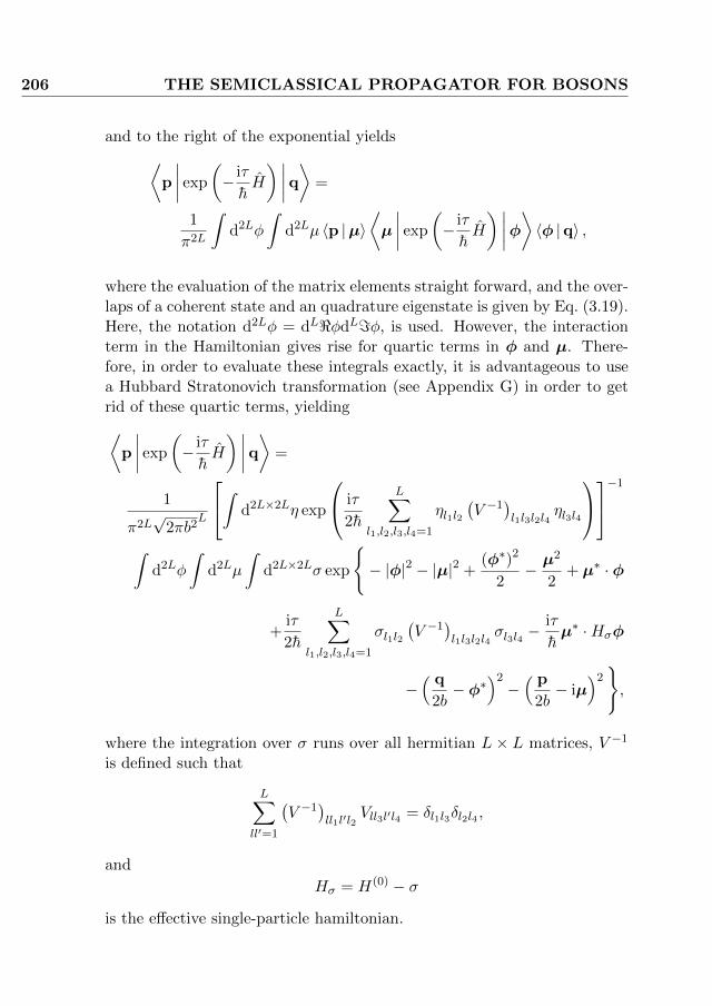
206 THE SEMICLASSICAL PROPAGATOR FOR BOSONS
and to the right of the exponential yields⟨p
∣∣∣∣ exp
(− iτ
hH
) ∣∣∣∣q⟩ =
1
π2L
∫d2Lφ
∫d2Lµ 〈p |µ〉
⟨µ
∣∣∣∣ exp
(− iτ
hH
) ∣∣∣∣φ⟩ 〈φ |q〉 ,where the evaluation of the matrix elements straight forward, and the over-laps of a coherent state and an quadrature eigenstate is given by Eq. (3.19).Here, the notation d2Lφ = dL<φdL=φ, is used. However, the interactionterm in the Hamiltonian gives rise for quartic terms in φ and µ. There-fore, in order to evaluate these integrals exactly, it is advantageous to usea Hubbard Stratonovich transformation (see Appendix G) in order to getrid of these quartic terms, yielding⟨
p
∣∣∣∣ exp
(− iτ
hH
) ∣∣∣∣q⟩ =
1
π2L√
2πb2L
∫ d2L×2Lη exp
iτ
2h
L∑l1,l2,l3,l4=1
ηl1l2(V −1
)l1l3l2l4
ηl3l4
−1
∫d2Lφ
∫d2Lµ
∫d2L×2Lσ exp
− |φ|2 − |µ|2 +
(φ∗)2
2− µ
2
2+ µ∗ · φ
+iτ
2h
L∑l1,l2,l3,l4=1
σl1l2(V −1
)l1l3l2l4
σl3l4 −iτ
hµ∗ ·Hσφ
−( q
2b− φ∗
)2−( p
2b− iµ
)2,
where the integration over σ runs over all hermitian L × L matrices, V −1
is defined such that
L∑ll′=1
(V −1
)ll1l′l2
Vll3l′l4 = δl1l3δl2l4 ,
and
Hσ = H(0) − σ
is the effective single-particle hamiltonian.

A.1. THE CLASSICAL HAMILTONIAN FOR BOSONIC SYSTEMS207
Performing the integrations over µ and φ is then cumbersome, butotherwise straight forward and yields
⟨p
∣∣∣∣ exp
(− iτ
hH
) ∣∣∣∣q⟩ =
1√
4πb2L
∫ d2L×2Lη exp
iτ
2h
L∑l1,l2,l3,l4=1
ηl1l2(V −1
)l1l3l2l4
ηl3l4
−1
∫d2L×2Lσ
exp
(iτ2h
L∑l1,l2,l3,l4=1
σl1l2(V −1
)l1l3l2l4
σl3l4
)√
det[IL − iτ
h<Hσ − τ2
2h2H∗σHσ
]
exp
− q2
4b2− p
4b2+
1
2b2
q−iq−ipp
A−1
q−iq−ipp
,
where the 4L× 4L-matrix A is given by
A =
3IL −iIL −IL + iτ
hH∗σ iIL + τ
hH∗σ
−iIL IL −iIL − τhH∗σ −IL + iτ
hH∗σ
−IL + iτhHσ −iIL − τ
hHσ IL −iILiIL + τ
hHσ −IL + iτhHσ −iIL 3IL
Since eventually τ will go to zero, the determinant in the denominator inthe third line can be approximated by an exponential,
det
[IL −
iτ
h<Hσ −
τ2
2h2H∗σHσ
]≈ det exp
[− iτ
h<Hσ
]= exp
[− iτ
hTrHσ
],
where the real part could be omitted in the last step, since Hσ is hermitian,and therefore its diagonal entries are real.
Moreover, the inverse of A can be approximated by its Taylor series up

208 THE SEMICLASSICAL PROPAGATOR FOR BOSONS
to first order in τ using (I4L + τX)−1 ≈ I4L − τX, which finally yields⟨p
∣∣∣∣ exp
(− iτ
hH
) ∣∣∣∣q⟩ =
1√
4πb2L
∫ d2L×2Lη exp
iτ
2h
L∑l1,l2,l3,l4=1
ηl1l2(V −1
)l1l3l2l4
ηl3l4
−1
∫d2L×2Lσ exp
iτ
2h
L∑l1,l2,l3,l4=1
σl1l2(V −1
)l1l3l2l4
σl3l4
− i
2b2p · q− iτ
hψ∗Hσψ +
iτ
2hTrHσ
Performing the integration over σ by substituting
σll′ = σ′ll′ +L∑
l1,l2=1
Vll1l′l2
[1
2δl1l2 − ψ∗l1ψl2
]yields ⟨
p
∣∣∣∣ exp
(− iτ
hH
) ∣∣∣∣q⟩ =
1√4πb2
exp
(− i
2b2p · q− iτ
hH(cl) (q− ip,q + ip)
),
where the classical Hamiltonian is given by Eq. (4.9).
A.2 The stationary phase approximation to thebosonic propagator in quadraturerepresentation
The stationary phase approximation to the propagator for bosonic sys-tems in quadrature representation starts from (c.f. Eq. (4.6))
K(q(f),q(i); tf , ti
)=
limM→∞
∫dLq(1) · · ·
∫dLq(M−1)
∫dLp(1) · · ·
∫dLp(M)
M∏m=1
1
(4πb2)L
exp
i
h
[h
2b2p(m)
(q(m) − q(m−1)
)− τH(cl)
(ψ(m)∗,ψ(m); ti +mτ
)],
A.2. THE STATIONARY PHASE APPROXIMATION 209
While the determination of the stationary points of the exponential isstraight forward and stated in section 4.3.1, the integration over fluctu-ations are more elaborate. These integrals are given by
limM→∞
∫dLδq(1) · · ·
∫dLδq(M−1)
∫dLδp(1) · · ·
∫dLδp(M) 1
(4πb2)MLexp
[iδp(1)δq(1)
2b2
+i
2b2
M∑m=2
(δq(m−1)
δp(m)
)(0 0IL 0
)(δq(m)
δp(m+1)
)− iτ
2hδp(1) ∂
2H(1)
∂p(1)2 δp(1)
− iτ
2h
M∑m=2
(δq(m−1)
δp(m)
) ∂2H(m)
∂q(m−1)2h
2b2τ+ ∂2H(m)
∂q(m−1)p(m)
h2b2τ
+ ∂2H(m)
∂p(m)q(m−1)∂2H(m)
∂p(m)2
( δq(m−1)
δp(m)
)],
which can after the substitutions δq(m) = 2bx(m), δp(m) = 2by(m) also bewritten as
limM→∞
∫dLx(1) · · ·
∫dLx(M−1)
∫dLy(1) · · ·
∫dLy(M) exp (iΦ/h)
πML (2b)L
× exp
iM−1∑m=1
[(x(m)
y(m)
) −2b2τh
∂2H(m+1)
∂q(m)2 ILIL −2b2τ
h∂2H(m)
∂p(m)2
( x(m)
y(m)
)
−2i
(x(m)
y(m)
)(0 IL + 2b2τ
h∂2H(m+1)
∂q(m)∂p(m+1)
0 0
)(x(m+1)
y(m+1)
)]
−2ib2τ
hy(M)∂
2H(M)
∂p(M)2 y(M)
,
where the result has to be evaluated at x(M) = 0.
Step by step integrating out x(1),y(1), x(2),y(2), x(3),y(3), . . . indicatesthat it is convenient to introduce recursively
X(m+1) =
− 2b2τ
h
∂2H(m+1)
∂p(m+1)2
+
(IL +
2b2τ
h
∂2H(m+1)
∂p(m+1)∂q(m)
)(−2b2τ
h
∂2H(m+1)
∂q(m)2 −X(m)−1
)−1
×(IL +
2b2τ
h
∂2H(m+1)
∂q(m)∂p(m+1)
)

210 THE SEMICLASSICAL PROPAGATOR FOR BOSONS
with the initial condition
X(1) = −2b2τ
h
∂2H(1)
∂p(1)2 .
Expanding Eq. (A.2) up to linear order in τ yields
X(m+1) = X(m) − 2b2τ
h
∂2H(m+1)
∂p(m+1)2 +2b2τ
h
∂2H(m+1)
∂p(m+1)∂q(m)X(m)
+2b2τ
hX(m) ∂2H(m+1)
∂q(m)∂p(m+1)− 2b2τ
hX(m)∂
2H(m+1)
∂q(m)2 X(m).
In continuous limit τ → 0, the recursion relation for X gets transformedinto a first order differential equation,
X = −2b2
h
∂2H
∂p2+
2b2
h
∂2H
∂p∂qX +
2b2
hX∂2H
∂q∂p− 2b2
hX∂2H
∂q2X
with initial condition X(ti) = 0 and is solved by
X = − ∂q
∂p(ti)
(∂p
∂p(ti)
)−1
Therefore, the integral over the fluctuations yields
limM→∞
∫dLy(M)
(2πb)Lexp
(iΦ/h+ iy(M)X(M)y(M)
)
×M−1∏m=1
[det i
(−2b2τ
h∂2H(m+1)
∂q(m)2 ILIL X(m)
)]− 12
= limM→∞
exp(
ihΦ)√
det(−4ib2πX(M)
) M−1∏m=1
[det
(IL +
2b2τ
h
∂2H(m+1)
∂q(m)2 X(m)
)]− 12
= limM→∞
exp(
ihΦ)√
det(−4ib2πX(M)
) exp
(−b
2τ
h
M−1∑m=1
Tr∂2H(m+1)
∂q(m)2 X(m)
)
=exp
(ihΦ)√
det (−4ib2πX(tf ))exp
−b2h
tf∫ti
dtTr∂2H
∂q2X
.
A.3. THE BASIS CHANGE FOR THE PROPAGATOR 211
Using the differential equation for ∂q/∂p(ti), the exponent can be writtenas
b2
h
tf∫ti
dtTr∂2H
∂q2X = −b
2
h
tf∫ti
dtTr∂2H
∂q2
∂q
∂p(ti)
(∂p
∂p(ti)
)−1
=1
2
tf∫ti
dtTr
(d
dt
∂p
∂p(ti)
)(∂p
∂p(ti)
)−1
+b2
h
tf∫ti
dtTr∂2H
∂q∂p
=1
2Tr ln
∂p(tf )
∂p(ti).
Thus, the semiclassical prefactor of the bosonic propagator in quadraturerepresentation is given by the van-Vleck-Gutzwiller determinant√
det
[1
−4ib2π
(−∂p(ti)
∂q(f)
)]=
√det
[1
−2πih
∂2Rγ
∂q(f)∂q(i)
].
A.3 The basis change from Quadratures to Fockstates for the semiclassical propagator
The propagator in Fock state representation is related to the propagatorin quadrature representation via
K(n(f),n(i); tf , ti
)= 〈n(f)| K (tf , ti) |n(i)〉
=
∫dLq(f)
∫dLq(i)
⟨n(f)
∣∣∣q(f)⟩〈q(f)| K (tf , ti) |q(i)〉
⟨q(i)
∣∣∣n(i)⟩
=
∫dLq(f)
∫Lq(i)
⟨n(f)
∣∣∣q(f)⟩⟨
q(i)∣∣∣n(i)
⟩K(q(f),q(i); tf , ti
).
We plug in the semiclassical propagator (4.10), as well as the asymptoticexpression of the overlap between a Fock and a quadrature state for largeoccupation number (3.13). Furthermore, for simplicity of writing, we in-troduce
F (q, n) =q
4b2
√4b2(n+
1
2
)− q2 −
(n+
1
2
)arccos
q
2b√n+ 1
2
+π
4,

212 THE SEMICLASSICAL PROPAGATOR FOR BOSONS
which can be interpreted as generating function for the basis transformfrom q and p to n and θ, where n is the modulus square and θ the phaseof the mean field wave function. This can be seen by noticing that,
∂F (q, n)
∂q=
√n+ 1
2 + q2
4b2
b≡ p
2b(A.1)
∂F (q, n)
∂n= − arccos
q
2b√n+ 1
2
≡ −θ. (A.2)
Using this definition, the semiclassical propagator in Fock state represen-tation can be written as
K(n(f),n(i); tf , ti
)=
∫dLq(f)
∫dLq(i)
∑s(i),s(f)∈−1,1L
L∏l=1
√√√√√∂2F(q
(f)l , n
(f)l
)∂q
(f)l ∂n
(f)l
∂2F(q
(i)l , n
(i)l
)∂q
(i)l ∂n
(i)l
×
∑γ:q(i)→q(f)
√det
1
(−8π3ih)
∂2Rγ(q(f),q(i); tf , ti
)∂q(f)∂q(i)
eihRγ(q(f),q(i);tf ,ti)
× exp
i
L∑l=1
[s
(i)l F
(q
(i)l , n
(i)l
)− s(f)
l F(q
(f)l , n
(f)l
)]+
i
hΦ (tf , ti)
.
(A.3)
Since the asymptotic formula for the overlap is valid only for the oscillating
region |q| < 2b√n+ 1
2 , one can substitute
q(i)1 =2b
√n
(i)1 +
1
2cos θ
(i)1 ,
q(i)l =2b
√n
(i)l +
1
2cos(θ
(i)l + θ
(i)1
)forl = 2, . . . , L,
q(f)l =2b
√n
(f)l +
1
2cos(θ
(f)l + θ
(i)1
)forl = 1, . . . , L.
In the following, for reasons that will become obvious after the stationary
phase conditions, we will refere to the θ(i/f)l ’s as “phases”. Note that these
definitions correspond to the definitions of the phases by (A.2). Together

A.3. THE BASIS CHANGE FOR THE PROPAGATOR 213
with the sums over s(i) and s(f), the integrals over θ(i/f)l then run from
−π to π and the phase θ(i)1 does not enter in the hamiltonian part of the
action. Moreover, it will turn out to be a global phase, dropping out of the
equations of motion. Therefore, the integral over θ(i)1 can not be evaluated
in stationary phase approximation, since it is an integral over a continuousfamily of trajectories.
However, the remaining 2L− 1 integrals can be evaluated in stationaryphase approximation. Here, we will do the two integrations over the finaland initial quadratures one after another, starting with the final ones.
The stationary phase condition for the integration over the final phasesis given by
p(f)l = 2b
√n
(f)l +
1
2sin(θ
(f)l + θ
(i)1
)Thus, the stationary phase approximation selects those classical trajectoriesψ(t) satisfying the boundary conditions
|ψl(tf )|2 = n(f)l +
1
2, (A.4)
and therefore justifies that we called the θ(f)l ’s “phases”, since the solutions
of the stationary phase conditions are the trajectories with the final phasesequal to them.
The evaluation of the exponent at the stationary point will be post-poned to when we derived the stationary phase condition for the initialphases.
The second derivative of the exponent in (A.3) with respect to the initialand final phases at the stationary point yields
∂2
∂θ(f)l ∂θ
(f)l′
1
hRγ
(q(f),q(i); tf , ti
)+
L∑m=1
[(n(f)m +
1
2
)(θ(f)m + θ
(i)1
)−√n
(f)m +
1
2cos(θ(f)m + θ
(i)1
)sin(θ(f)m + θ
(i)1
)]
=
√n
(f)l +
1
2sin(θ
(f)l + θ
(i)1
)[2δll′
√n
(f)l +
1
2cos(θ
(f)l + θ
(i)1
)− 1
b
∂p(f)l
∂θ(f)l′
]
= − ∂
∂θ(f)l′
1
4b2
[(q
(f)l
)2+(p
(f)l
)2]
= −(∂θ
(f)l′
∂n(f)l
)−1
.

214 THE SEMICLASSICAL PROPAGATOR FOR BOSONS
Therefore, together with the prefactor given by the second derivative ofthe generating function, the semiclassical prefactor after performing theintegration over the final phases is given by√√√√ L∏
l=1
∂q(i)l
∂θ(i)l
√1
(−4π2ih)Ldet
∂2Rγ(n(f),q(i); tf , ti
)∂n(f)∂q(i)
, (A.5)
where we defined
Rγ
(n(f),q(i); tf , ti
)=
Rγ
(q(f),q(i); tf , ti
)+ h
L∑l=1
[(n
(f)l +
1
2
)(θ
(f)l + θ
(i)1
)−√n
(f)l +
1
2cos(θ
(f)l + θ
(i)1
)sin(θ
(f)l + θ
(i)1
)]evaluated at the stationary point.
Noticing that
∂Rγ(n(f),q(i); tf , ti
)∂n(f)
= h(θ(f) + θ
(i)1 1),
where 1 is the vector, which every entry is equal to one, one can write (A.5)also as √√√√
det1
(−4π2i)
∂(θ(f) + θ
(i)1 1)
∂θ(i).
Now, the stationary phase condition for the integration over the initial
phases, save for θ(i)1 , yields
p(i)l = 2b
√n
(i)l +
1
2sin(θ
(i)l + θ
(i)1
),
which corresponds to
|ψl(ti)|2 = n(i)l +
1
2. (A.6)
Note that with (A.4) and (A.6) the conservation of the total number of par-
ticles together with the fact that q(i)1 =
√n
(i)1 + 1/2 cos θ
(i)1 already requires
that
ψ1(ti) =
√n
(i)1 +
1
2exp
(iθ
(i)1
). (A.7)
A.3. THE BASIS CHANGE FOR THE PROPAGATOR 215
Moreover, we see that θ(i)1 indeed is a global phase, which does neither enter
the equations of motion, nor the Hamiltonian. Therefore, the solutions tothe equations of motion under the boundary conditions (A.4), (A.6) and(A.7) are the trajectories with the initial phase of the first componentfixed to a certain ϕ, e.g. ϕ = 0, and multiplied by a global phase factor
exp(
iθ(i)1 − iϕ
).
With this, one can now evaluate the exponent at the stationary points,which will then give the classical action in Fock representation. Substitut-ing
ql(t) =2b
√nl(t) +
1
2cos(θl(t) + θ
(i)1
),
pl(t) =2b
√nl(t) +
1
2sin(θl(t) + θ
(i)1
)
in the kinetic part of the action, in consideration of the preservation of thetotal number of particles by the classical equations of motion yields for theclassical action in Fock state representation
Rγ
(n(f),n(i); tf , ti
)=
tf∫ti
dt[hθ(t) · n(t)−H(cl) (ψ∗(t),ψ(t); t)
].
Analoguous to above,
∂2
∂θ(i)l ∂θ
(i)l′
1
hR(n(f),q(i); tf , ti
)−
L∑m=1
[(n(i)m +
1
2
)(θ(i)m + θ
(i)1
)−√n
(i)m +
1
2cos(θ(i)m + θ
(i)1
)sin(θ(i)m + θ
(i)1
)]
=
(∂θ
(i)l′
∂n(i)l
)−1
.
216 THE SEMICLASSICAL PROPAGATOR FOR BOSONS
Therefore, we find
K(n(f),n(i); tf , ti
)=
1
2π
2π∫0
dθ(i)1
∑γ:n(f)→n(i)
√√√√√ 1
−2πidet
(∂θ
(i)l
∂n(i)l′
)l,l′=2,...,L
det∂(θ(f) + θ
(i)1 1)
∂θ(i)
× exp
[i
hRγ
(n(f),n(i); tf , ti
)+
i
hΦ (tf , ti)
].
(A.8)
It is important to notice that the two matrices in the prefactor have differentdimensions. The first one is a (L − 1) × (L − 1)-matrix, while the second
one is L×L dimensional. However, since θ(f) does not depend on θ(i)1 , the
second one has the form (1
∂θ(f)
∂θ(i),
)where θ
(i)is the vector resulting from θ(i) by skipping its first entry. More-
over, we can match the dimensions of the two matrices by using
det
(∂θ
(i)
∂n(i)
)= det
(1 0
0 ∂˜θ
(i)
∂n(i)
)Then, (
1∂θ(f)
∂θ(i),
)(1 0
0 ∂˜θ
(i)
∂n(i)
)=
(1
∂θ(f)
∂n(i)
).
The determinant of this matrix however can be further simplified by usingSylvester’s determinant theorem, which states that for an n×m matrix Aand an m× n matrix B
det (In +AB) = det (Im +BA) ,
where In is the n× n unit matrix and applying it to the right hand side of
det
1∂θ
(f)1
∂n(i)
1 ∂˜θ
(f)
∂n(i)
=
det
1∂θ
(f)1
∂n(i)
0 ∂˜θ
(f)
∂n(i)
IL +
−∂θ
(f)1
∂n(i)
(∂
˜θ(f)
∂n(i)
)−1
1 0T(∂
˜θ(f)
∂n(i)
)−1
1 0

A.3. THE BASIS CHANGE FOR THE PROPAGATOR 217
With this, one can show that
det
(1
∂θ(f)
∂n(i)
)= det
∂θ(f)
∂n(i)= det h
∂2Rγ(n(f),n(i); tf , ti
)∂n(f)∂n(i)
.
Finally, we see that the integrand in (A.8) is independent of θ(i)1 , such that
the final result reads
K(n(f),n(i); tf , ti
)=
∑γ:n(i)→n(f)
√det
1
(−2πih)
∂2Rγ(n(f),n(i); tf , ti
)∂n(f)∂n(i)
× exp
i
h
[Rγ
(n(f),n(i); tf , ti
)+ Φ (tf , ti)
].


APPENDIX BThe Feynman Path Integralfor Fermions using complex
variables
The starting point for the derivation of a complex path integral represen-tation of the fermionic propagator is, cf. (5.1)
K(n(f),n(i); tf , ti
)=
limM→∞
∫d2Lζ(0)
∫d2Lχ(0) · · ·
∫d2Lζ(M)
∫d2Lχ(M)
⟨n(f)
∣∣∣χ(M)⟩
×⟨χ(M)
∣∣∣ ζ(M)⟩M−1∏
m=0
〈ζ(m+1)| e− iτhH(m) |χ(m)〉
⟨χ(m)
∣∣∣ ζ(m)⟩
×⟨ζ(0)
∣∣∣n(i)⟩,
219

220 THE COMPLEX PATH INTEGRAL FOR FERMIONS
which after expanding the exponential up to first order in τ and evaluatingthe overlaps yields
K(n(f),n(i); tf , ti
)=
limM→∞
∫d2Lζ(0)
∫d2Lχ(0) · · ·
∫d2Lζ(M)
∫d2Lχ(M)
[L−1∏l=0
(χ
(M)L−l
)n(f)L−l
]
× exp
[−
M∑m=0
(ζ(m)∗ · ζ(m) + χ(m)∗ · χ(m)
)][ L∏l=1
(1 + χ
(M)l
∗ζ
(M)l
)]
×
M−1∏m=0
1− iτ
h
L∑α,β=1
(h
(m)αβ ζ
(m+1)α
∗χ
(m)β + U
(m)αβ ζ(m+1)
α
∗ζ
(m+1)β
∗χ
(m)β χ(m)
α
)×[L∏l=1
(1 + ζ
(m+1)l
∗χ
(m)l
)(1 + χ
(m)l
∗ζ
(m)l
)]
×[L∏l=1
(ζ
(0)l
∗)n(i)l
].
The fact that for (positiv) integer j, j′
2π∫0
dθ
∫d2φ exp
(− |φ|2 + φ∗eiθ − ijθ
)φj′
=2π2δj,j′ (B.1a)
∫d2φ
∫d2µ exp
(− |φ|2 − |µ|2 + φ∗µ
)φj (µ∗)j
′=π2j! δj,j′ , (B.1b)
where d2µ = d<µd=µ, allows to insert these integrals such that ζ(m+1) andζ(m) appear decoupled only. For this, it is best to first of all expand thefactors of the product over the individual time steps according to[
L∏l=1
(1 + χ
(m)l
∗ζ
(m)l
)]
×
1− iτ
h
L∑α,β=1
(h
(m−1)αβ ζ(m)
α
∗χ
(m−1)β + U
(m−1)αβ ζ(m)
α
∗ζ
(m)β
∗χ
(m−1)β χ(m−1)
α
)=
[a(m) − iτ
hb(m) − iτ
hc(m) − iτ
hd(m)
],

THE COMPLEX PATH INTEGRAL FOR FERMIONS 221
with
a(m) =L∏l=1
(1 + χ
(m)l
∗ζ
(m)l
)b(m) = Θ (m− 1)
[L∏l=1
(1 + χ
(m)l
∗ζ
(m)l
)] L∑α=1
h(m−1)αα ζ(m)
α χ(m−1)α
c(m) = Θ (m− 1)
[L∏l=1
(1 + χ
(m)l
∗ζ
(m)l
)] L∑α,β=1α 6=β
h(m−1)αβ ζ(m)
α χ(m−1)β
d(m) =
Θ(m− 1)
[L∏l=1
(1 + χ
(m)l
∗ζ
(m)l
)] L∑α,β=1α 6=β
U(m−1)αβ ζ(m)
α ζ(m)β χ
(m−1)β χ(m−1)
α
and then considering one by one each factor starting with m = 0. Form = 0, (B.1a) is used in order to replace
∫d2Lζ(0) exp
(−ζ(0)∗ · ζ(0)
)[ L∏l=1
(1 + χ
(0)l
∗ζ
(0)l
)] L∏l=1
(ζ
(0)l
∗)n(i)l
=
∫d2N(i)
φ(0)
2π∫0
dN(i)θ(i)
∫d2Lζ(0)e−ζ
(0)∗·ζ(0)−|φ(0)|2+φ(0)∗·µ(0)
×[L∏l=1
(1 + χ
(0)l
∗φ
(0)l
)][L−1∏l=0
(1 + ζ
(0)L−lµ
(0)L−l∗)] L∏
l=1
(ζ
(0)l
∗)n(i)l
(2π2)N(i)
,
with µ(0)l = n
(i)l exp
(iθ
(i)l
)for all l ∈ 1, . . . , L. Note that here, for the
initially unoccupied sites, the phases θ(i)l are arbitrary but fixed, e.g. to
zero.
For the N (i) =∑L
l=1 n(i)l occupied sites, the identity follows directly
from (B.1a), while for the unoccupied ones, it is important to notice that
the term χ(0)l
∗ζ
(0)l does vanish when integrating over ζ(0). This is because
of the properties of the Grassmann integrals (3.20) and the fact that there
is no ζ(0)l
∗for those components, for which n
(i)l = 0.

222 THE COMPLEX PATH INTEGRAL FOR FERMIONS
For m > 0, using (B.1b) leads to
a(m) =
∫d2Lµ(m)
∫ 2Lφ(m)
π2Le−|φ(m)|2−|µ(m)|2+φ(m)∗·µ(m)
×[L∏l=1
(1 + χ
(m)l
∗φ
(m)l
)] L−1∏l=0
1 + ζ(m)L−l
∞∑j=1
1
j!
(µ
(m)L−l∗)j (
φ(m−1)L−l
)j−1
b(m) =
∫d2Lµ(m)
∫ 2Lφ(m)
π2Le−|φ(m)|2−|µ(m)|2+φ(m)∗·µ(m)
[L∏l=1
(1 + χ
(m)l
∗φ
(m)l
)]
×L∑α=1
h(m−1)αα ζ(m)
α
∗χ(m−1)α
L−1∏l=0
1 + ζ(m)L−l
∞∑j=1
(µ
(m)L−l∗)j (
φ(m−1)L−l
)j−1
(j − δL−l,α) !
c(m) =
∫d2Lµ(m)
∫ 2Lφ(m)
π2Le−|φ(m)|2−|µ(m)|2+φ(m)∗·µ(m)
×[L∏l=1
(1 + χ
(m)l
∗φ
(m)l
)] L∑α,β=1α6=β
h(m−1)αβ ζ(m)
α
∗χ
(m−1)β
×
L−max(α,β)−1∏
l=0
1 + ζ(m)L−l
∞∑j=1
1
j!
(µ
(m)L−l∗)j (
φ(m−1)L−l
)j−1
×(
1 + ζ(m)max(α,β)µ
(m)max(α,β)
∗)×
L−min(α,β)−1∏l=L−max(α,β)+1
1 + ζ(m)L−l
∞∑j=1
2j − 1
j!
(µ
(m)L−l∗)j (
φ(m−1)L−l
)j−1
×(
1 + ζ(m)min(α,β)µ
(m)min(α,β)
∗)×
L−1∏l=L−min(α,β)+1
1 + ζ(m)L−l
∞∑j=1
1
j!
(µ
(m)L−l∗)j (
φ(m−1)L−l
)j−1
d(m) =
∫d2Lµ(m)
∫ 2Lφ(m)
π2Le−|φ(m)|2−|µ(m)|2+φ(m)∗·µ(m)
×[L∏l=1
(1 + χ
(m)l
∗φ
(m)l
)] L∑α,β=1α6=β
U(m−1)αβ ζ(m)
α
∗ζ
(m)β
∗χ
(m−1)β χ(m−1)
α
×L−1∏l=0
1 + ζ(m)L−l
∞∑j=1
1
(j − δL−l,α − δL−l,β) !
(µ
(m)L−l∗)j (
φ(m−1)L−l
)j−1

THE COMPLEX PATH INTEGRAL FOR FERMIONS 223
It has been possible to insert the additional terms(φ
(m−1)l
)j−1, since these
variables are already defined by the integrals introduced for smaller m, andthe integration over µ(m) and φ(m) selects the j = 1 term only.
Finally, for m = M , a similar argument as for m = 0 allows to restrict
the integrals over φ(M) again to those N (f) =∑L
l=1 n(f)l components with
n(f)l = 1, while setting all the other components of φ(M) to zero.

224 THE COMPLEX PATH INTEGRAL FOR FERMIONS
After this, the propagator reads
K(n(f),n(i); tf , ti
)=
limM→∞
∫d2Lζ(0)
∫d2Lχ(0) · · ·
∫d2Lζ(M)
∫d2Lχ(M)
2π∫0
dN(i)
θ(i)
∫d2Lφ(0)
∫d2Lφ(1)
∫d2Lµ(1) · · ·
∫d2Lφ(M−1)
∫d2Lµ(M−1)
∫d2Lµ(M)
∫d2N(f)
φ(M)
e
M∑m=0
[−ζ(m)∗·ζ(m)−χ(m)∗·χ(m)−|φ(m)|2−|µ(m)|2+φ(m)∗·µ(m)
]+N(i)
× 1
2N(i)πN(i)+N(f)+2ML
[L−1∏l=0
(χ
(M)L−l
)n(f)L−l
][L∏l=1
(1 + χ
(M)l
∗φ
(M)l
)]
×
M−1∏m=0
[L−1∏l=0
(1 + ζ
(m+1)L−l
∞∑j=1
1
j!
(µ
(m+1)L−l
∗)j (φ
(m)L−l
)j−1)
− iτ
h
L∑α=1
h(m)αα ζ
(m+1)α
∗χ(m)α
L−l∏l=0
1 + ζ(m+1)L−l
∞∑j=1
(µ
(m+1)L−l
∗)j (φ
(m)L−l
)j−1
(j − δL−l,α) !
− iτ
h
L∑α,β=1α 6=β
h(m)αβ ζ
(m+1)α
∗χ
(m)β
×
L−max(α,β)−1∏l=0
1 + ζ(m+1)L−l
∞∑j=1
(µ
(m+1)L−l
∗)j (φ
(m)L−l
)j−1
j!
×(
1 + ζ(m+1)
max(α,β)µ(m+1)
max(α,β)
∗)×
L−min(α,β)−1∏l=L−max(α,β)+1
1 + ζ
(m+1)L−l
∞∑j=1
2j − 1
j!
(µ
(m+1)L−l
∗)j (φ
(m)L−l
)j−1
×(
1 + ζ(m+1)
min(α,β)µ(m+1)
min(α,β)
∗)×
L−1∏l=L−min(α,β)+1
(1 + ζ
(m+1)L−l
∞∑j=1
1
j!
(µ
(m+1)L−l
∗)j (φ
(m)L−l
)j−1)
− iτ
h
L∑α,β=1α 6=β
U(m)αβ ζ(m+1)
α
∗ζ
(m+1)β
∗χ
(m)β χ(m)
α
×L−l∏l=0
1 + ζ(m+1)L−l
∞∑j=1
(µ
(m+1)L−l
∗)j (φ
(m)L−l
)j−1
(j − δL−l,α − δL−l,β) !
[ L∏
l=1
(1 + ζ
(m+1)l
∗χ
(m)l
)]
×L∏l=1
[1 + χ
(m)l
∗φ
(m)l
][L−1∏l=0
(1 + ζ
(0)L−lµ
(0)L−l∗)] L∏
l=1
(ζ
(0)l
∗)n(i)l,

THE COMPLEX PATH INTEGRAL FOR FERMIONS 225
with µ(0)l = n
(i)l exp
(iθ
(i)l
).
Since the m-th factor in the product over the timesteps only depends onζ(m+1) and χ(m), one can easily integrate out the intermediate Grassmann

226 THE COMPLEX PATH INTEGRAL FOR FERMIONS
variables ζ(1), . . . , ζ(M) and χ(0), . . . ,χ(M−1) by using∫d2Lζ(m+1)
∫d2Lχ(m)e−ζ
(m+1)∗·ζ(m+1)−χ(m)∗·χ(m)
×[L−1∏l=0
(1 + ζ
(m+1)L−l f
(m)L−l
)][ L∏l=1
(1 + ζ
(m+1)l
∗χ
(m)l
)]
×L∏l=1
(1 + χ
(m)l
∗φ
(m)l
)=
L∏l=1
(1 + f
(m)l φ
(m)l
),
∫d2Lζ(m+1)
∫d2Lχ(m)e−ζ
(m+1)∗·ζ(m+1)−χ(m)∗·χ(m)ζ(m+1)α
∗χ
(m)β
×[L−1∏l=0
(1 + ζ
(m+1)L−l f
(m)L−l
)][ L∏l=1
(1 + ζ
(m+1)l
∗χ
(m)l
)]
×L∏l=1
(1 + χ
(m)l
∗φ
(m)l
)
= f (m)α φ
(m)β
min(α,β)−1∏l=1
(1 + f
(m)l φ
(m)l
)×
L∏l=max(α,β)+1
(1 + f
(m)l φ
(m)l
) max(α,β)−1∏l=min(α,β)+1
(1− f (m)
l φ(m)l
),
∫d2Lζ(m+1)
∫d2Lχ(m)e−ζ
(m+1)∗·ζ(m+1)−χ(m)∗·χ(m)ζ(m+1)α
∗ζ
(m+1)β
∗
× χ(m)β χ(m)
α
[L−1∏l=0
(1 + ζ
(m+1)L−l f
(m)L−l
)][ L∏l=1
(1 + ζ
(m+1)l
∗χ
(m)l
)]
×L∏l=1
(1 + χ
(m)l
∗φ
(m)l
)= f (m)
α f(m)β φ
(m)β φ(m)
α
l∏l=1l 6=α,β
(1 + f
(m)l φ
(m)l
).

THE COMPLEX PATH INTEGRAL FOR FERMIONS 227
Moreover, the integrals over ζ(0) and χ(M) yield
∫d2Lζ(0)e−ζ
(0)∗·ζ(0)
[L−1∏l=0
(1 + ζ
(0)L−lµ
(0)L−l∗)] L∏
l=1
(ζ
(0)l
∗)n(i)l
=
N(i)∏j=1
µ(0)
l(i)j
∗
∫d2Lχ(M)e−χ
(M)∗·χ(M)
[L−1∏l=0
(χ
(M)L−l
)n(f)L−l
]L∏l=1
(1 + χ
(M)l φ
(M)l
∗)=
N(f)∏j=1
φ(M)
l(f)j
After performing these integrals, one notices that the inserted integralshave been chosen such that the resulting sums can be performed, yieldingexponentials, and finds the propagator to read
K(n(f),n(i); tf , ti
)=
limM→∞
∫d2Lφ(0)
∫d2Lφ(1)
∫d2Lµ(1) · · ·
∫d2Lφ(M−1)
∫d2Lµ(M−1)
∫d2Lµ(M)
∫d2N(f)
φ(M)
2π∫0
dN(i)θ(i)
N(f)∏j=1
φ(M)
l(f)j
exp
M∑m=0
[−∣∣∣φ(m)
∣∣∣2
−∣∣∣µ(m)
∣∣∣2 + φ(m)∗ · µ(m)
]+N (i) − i
N(i)∑j=1
θ(i)
l(i)j
+
M−1∑m=0
µ(m+1)∗ · φ(m)
×
M−1∏m=0
[1− iτ
hH(cl)(k)
(µ(m+1)∗,φ(m)
)]2N
(i)πN
(i)+N(f)+2ML,

228 THE COMPLEX PATH INTEGRAL FOR FERMIONS
with
H(cl)(k) (µ∗,φ) =
L∑α=1
h(k)ααµ
∗αφα +
L∑α,β=1α 6=β
U(k)αβ µ
∗αµ∗βφβφα
+
L∑α,β=1α 6=β
h(k)αβµ
∗αφβ exp
(−µ∗αφα − µ∗βφβ
) max(α,β)−1∏l=min(α,β)+1
(1− 2µ∗l φl) .
Now, one can also integrate out µ(1), . . . ,µ(M) as well as φ(0) and redo theexpansion in τ to obtain the final path integral expression,
K(n(f),n(i); tf , ti
)=
limM→∞
2π∫0
dN(i)θ(i)
∫d2Lφ(1) · · ·
∫d2Lφ(M−1)
∫d2N(f)
φ(M)
N(f)∏j=1
φ(M)
l(f)j
e
M∑m=1
[−|φ(m)|2+φ(m)∗·φ(m−1)− iτ
hH(cl)(m−1)
(φ(m)∗,φ(m−1))]−i
N(i)∑j=1
θ(i)
l(i)j
(2π)N(i)πN
(f)+(M−1)L.
APPENDIX CSemiclassical propagator for
Fermions
C.1 Derivation of the semiclassical prefactor
After the substitution φ(m)l =
√J
(m)l exp
[i
(θ
(m)l − θ(i)
l(i)1
)]and integra-
tion over θ(i)
l(i)1
, the propagator is given by
K(n(f),n(i); tf , ti
)=
δN(i),N(f) limM→∞
2π∫0
dN−1θ(i)
2π∫0
dLθ(1)
∞∫0
dLJ (1) · · ·2π∫0
dLθ(M−1)
∞∫0
dLJ (M−1)
2π∫0
dNθ(M)
∞∫0
dNJ (M)exp
[i(n(f) · θ(M) − n(i)θ(i)
)](2π)2N−1+(M−1)L
N∏j=1
√J
(M)
l(f)j
exp
M∑m=1
[−∣∣∣φ(m)
∣∣∣2 + φ(m)∗ · φ(m−1) − iτ
hH(cl)(m−1)
(φ(m)∗,φ(m−1)
)],
where now (and in the following) θ(i)
l(i)1
= 0. For simplicity of writing the
initial and final phases for the non-occupied states are also set to zero,
i.e. θ(i)l = 0 for all l ∈ 1, . . . , L\
l(i)2 , . . . , l
(i)
N(i)
as well as θ
(f)l = 0 for all
229

230 SEMICLASSICAL PROPAGATOR FOR FERMIONS
l ∈ 1, . . . , L \l(f)1 , . . . , l
(f)
N(f)
. When performing the stationary phase
approximation, the additional factor
N∏j=1
√J
(M)
l(f)j
= exp
1
2
N∑j=1
log J(M)
l(f)j
has to be included in the stationary phase analysis as well.
The stationary phase conditions are then found by taking the derivative
of the exponent with respect to all the J(m)l and θ
(m)l individually and are
given by
− exp
(−iθ
(i)
l(i)j
)+ φ
(1)
l(i)j
∗− iτ
h
∂H(cl)(0)
∂φ(0)
l(i)j
= 0
(φ
(m−1)l − iτ
h
∂H(cl)(m−1)
∂φ(m)l
∗
)∂φ
(m)l
∗
∂J(m)l
+
(φ
(m+1)l
∗− iτ
h
∂H(cl)(m)
∂φ(m)l
)∂φ
(m)l
∂J(m)l
= 1(φ
(m−1)l − iτ
h
∂H(cl)(m−1)
∂φ(m)l
∗
)∂φ
(m)l
∗
∂θ(m)l
+
(φ
(m+1)l
∗− iτ
h
∂H(cl)(m)
∂φ(m)l
)∂φ
(m)l
∂θ(m)l
= 0 1√J
(M)
l(f)j
− 2
√J
(M)
l(f)j
exp
(iθ
(M)
l(f)j
)+ φ
(M−1)
l(f)j
− iτ
h
∂H(cl)(M−1)
∂φ(M)
l(f)j
∗ = 0
exp
(iθ
(M)
l(f)j
)√J
(M)
l(f)j
−
φ(M−1)
l(f)j
− iτ
h
∂H(cl)(M−1)
∂φ(M)
l(f)j
∗
= 0
with the short hand notation H(cl)(m)= H(cl)(m)
(φ(m+1)∗,φ(m)
). The
second and third equation are found for all m ∈ 1, . . . ,M − 1. Keeping
in mind that φ(0)l = n
(i)l exp
(iθ
(i)l
), these stationary phase conditions can
be written as
φ(m)−φ(m−1)
τ = − ih∂H(cl)(m−1)
∂φ(m)∗ 1 ≤ m ≤M
φ(m)∗−φ(m−1)∗
τ = ih∂H(cl)(m−1)
∂φ(m−1) 1 ≤ m ≤M
J(M)
l(f)j
= n(f)
l(f)j
.

C.1. DERIVATION OF THE SEMICLASSICAL PREFACTOR 231
Therefore, in the continuous limit τ → 0, the stationary phase approxima-tion selects the classical trajectories from n(i) to n(f), which are defined asthe solutions of the equations of motion
ihφ =∂H(cl)
∂φ∗.
with
H(cl) =
L∑α=1
hαα(t) |φα(t)|2 +L∑
α,β=1α 6=β
Uαβ(t) |φα(t)|2 |φβ(t)|2
+L∑
α,β=1α6=β
hαβ(t)φ∗α(t)φβ(t)e−|φα(t)|2−|φβ(t)|2max(α,β)−1∏l=min(α,β)+1
(1− 2 |φl(t)|2
)
under the boundary conditions
|φl (ti)|2 =n(i)l
|φl (tf )|2 =n(f)l
and φl(i)1
(ti) = 1.
The semiclassical propagator in Fock state representation for Fermionsis then given by a sum over these classical trajectories,
K(n(f),n(i); tf , ti
)=
∑γ:n(i)→n(f)
exp
(i
hRγ
)K
(γ)red ,
with the classical action
Rγ =
tf∫ti
dt[hθ(t) · J(t)−H(cl) (φ∗(t),φ(t); t)
].
The reduced propagator is given by the remaining integrals over the fluc-

232 SEMICLASSICAL PROPAGATOR FOR FERMIONS
tuations,
K(γ)red =
limM→∞
1
(2π)2N−1+(M−1)L
∫dN−1δθ(0)
∫dNδJ (M)
∫dNδθ(M)
∫dLδJ (1)
∫dLδθ(1) · · ·
∫dLδJ (M−1)
∫dLδθ(M−1)
exp
−1
2δθ(0)P
(i)0
(A
(0)1 + C
(0)1
)P
(i)0
Tδθ(0)
− 1
2
(δθ(M)P (f)
δJ(M)P (f)
)(B
(M)1 +D
(M)1 B
(M)2 +D
(M)2
B(M)2 +D
(M)2
TB
(M)3 +D
(M)3
)(P (f)T
δθ(M)
P (f)TδJ(M)
)
− 1
2
M−1∑m=1
(δθ(m)
δJ(m)
)[(A
(m)1 +B
(m+1)1 A
(m)2 −B(m+1)
2
A(m)2 −B(m+1)
2 A(m)3 +B
(m+1)3
)
+
(C
(m)1 +D
(m)1 C
(m)2 +D
(m)2
C(m)2
T+D
(m)2
TC
(m)3 +D
(m)3
)](δθ(m)
δJ(m)
)
+
(δθ(1)
δJ(1)
)(E
(0)1
E(0)3
)P
(i)0
Tδθ(0)
+
(δθ(M)P (f)
δJ(M)P (f)
)(E
(M−1)1 E
(M−1)2
E(M−1)3 E
(M−1)4
)(δθ(m)
δJ(m)
)
+
M−2∑m=1
(δθ(m+1)
δJ(m+1)
)(E
(m)1 E
(m)2
E(m)3 E
(m)4
)(δθ(m)
δJ(m)
)(C.1)
where P (i/f) and P(i/f)0 are defined in the same way as in section 5.2.2,
namely as the (N −1)×L and, respectively, N ×L-matrices, which projectonto the subspace of initially and finally occupied sites, with the latterexcluding the first occupied one,(
P (i/f))jl′
=δl(i/f)j ,l′(
P(i/f)0
)jl′
=δl(i/f)j+1 ,l′
For later reference, their complements P (i/f) and P(i/f)0 are also defined,
as well as
Q(i/f) =
(P (i/f)
P (i/f)
)

C.1. DERIVATION OF THE SEMICLASSICAL PREFACTOR 233
which are the (orthogonal) matrices, which put the components corre-sponding to initially and finally unoccupied sites, respectively to the firstL − N (i/f) positions, and those correspondig to occupied sites to the lastN (i/f) positions, see (5.11).
Furthermore,
(A
(m)1
)ll′
=δll′φ(m)l
[φ
(m+1)l
∗− iτ
h
∂H(cl)(m)
∂φ(m)l
](A
(m)2
)ll′
=δll′iφ
(m)l
2J(m)l
[φ
(m+1)l
∗− iτ
h
∂H(cl)(m)
∂φ(m)l
](A
(m)3
)ll′
=δll′φ
(m)l
4J(m)l
2
[φ
(m+1)l
∗− iτ
h
∂H(cl)(m)
∂φ(m)l
](B
(m)1
)ll′
=δll′φ(m)l
∗[φ
(m−1)l − iτ
h
∂H(cl)(m−1)
∂φ(m)l
∗
](B
(m)2
)ll′
=δll′iφ
(m)l
∗
2J(m)l
[φ
(m−1)l − iτ
h
∂H(cl)(m−1)
∂φ(m)l
∗
](B
(m)3
)ll′
=δll′φ
(m)l
∗
4J(m)l
2
[2n
(f)l δm,M + φ
(m−1)l − iτ
h
∂H(cl)(m−1)
∂φ(m)l
∗
](C
(m)1
)ll′
=iτ
h
∂φ(m)l
∂θ(m)l
∂2H(cl)(m)
∂φ(m)l φ
(m)l′
∂φ(m)l′
∂θ(m)l′(
C(m)2
)ll′
=iτ
h
∂φ(m)l
∂θ(m)l
∂2H(cl)(m)
∂φ(m)l φ
(m)l′
∂φ(m)l′
∂J(m)l′(
C(m)3
)ll′
=iτ
h
∂φ(m)l
∂J(m)l
∂2H(cl)(m)
∂φ(m)l φ
(m)l′
∂φ(m)l′
∂J(m)l′

234 SEMICLASSICAL PROPAGATOR FOR FERMIONS
as well as
(D
(m)1
)ll′
=iτ
h
∂φ(m)l
∗
∂θ(m)l
∂2H(cl)(m−1)
∂φ(m)l
∗φ
(m)l′∗∂φ
(m)l′∗
∂θ(m)l′(
D(m)2
)ll′
=iτ
h
∂φ(m)l
∗
∂θ(m)l
∂2H(cl)(m−1)
∂φ(m)l
∗φ
(m)l′∗∂φ
(m)l′∗
∂J(m)l′(
D(m)3
)ll′
=iτ
h
∂φ(m)l
∗
∂J(m)l
∂2H(cl)(m−1)
∂φ(m)l
∗φ
(m)l′∗∂φ
(m)l′∗
∂J(m)l′(
E(m)1
)ll′
=∂φ
(m+1)l
∗
∂θ(m+1)l
[δll′ −
iτ
h
∂2H(cl)(m)
∂φ(m+1)l
∗∂φ
(m)l′
]∂φ
(m)l′
∂θ(m)l′(
E(m)2
)ll′
=∂φ
(m+1)l
∗
∂θ(m+1)l
[δll′ −
iτ
h
∂2H(cl)(m)
∂φ(m+1)l
∗∂φ
(m)l′
]∂φ
(m)l′
∂J(m)l′(
E(m)3
)ll′
=∂φ
(m+1)l
∗
∂J(m+1)l
[δll′ −
iτ
h
∂2H(cl)(m)
∂φ(m+1)l
∗∂φ
(m)l′
]∂φ
(m)l′
∂θ(m)l′(
E(m)4
)ll′
=∂φ
(m+1)l
∗
∂J(m+1)l
[δll′ −
iτ
h
∂2H(cl)(m)
∂φ(m+1)l
∗∂φ
(m)l′
]∂φ
(m)l′
∂J(m)l′
.
These matrices have to be evaluated at the stationary points, whichmeans that one can use the equations of motion to simplify
(A
(m)1
)ll′
=(B
(m)1
)ll′
=δll′J(m)l(
A(m)2
)ll′
=(B
(m)2
)ll′
=δll′i
2(A
(m)3
)ll′
=(B
(m)3
)ll′
=δll′1
4J(m)l

C.1. DERIVATION OF THE SEMICLASSICAL PREFACTOR 235
With this, (C.1) can be written as
K(γ)red =
limM→∞
1
(2π)2N−1+(M−1)L
∫dN−1
δθ(0)∫
dNδJ
(M)∫
dNδθ
(M)
∫dLδJ
(1)∫
dLδθ
(1) · · ·∫
dLδJ
(M−1)∫
dLδθ
(M−1)
exp
−
1
2δθ
(0)P
(i)0
∂φ(0)
∂θ(i)
[−e−2idiag
(θ(i)
)+
iτ
h
∂2H(cl)(0)
∂φ(0)2
]∂φ(0)
∂θ(i)P
(i)0
Tδθ
(0)
−1
2
(δθ(M)P (f)
δJ(M)P (f)
)O(M)T
e−2idiag
(θ(M)
)IL
IL iτh∂2H(cl)(M−1)
∂φ(M)∗2
O(M)
(P (f)T
δθ(M)
P (f)TδJ(M)
)
−1
2
M−1∑m=1
(δθ(m)
δJ(m)
)O(m)T
iτh∂2H(cl)(m)
∂φ(m)2 IL
IL iτh∂2H(cl)(m−1)
∂φ(m)∗2
O(m)
(δθ(m)
δJ(m)
)
+
(δθ(1)
δJ(1)
)O(1)T
0
IL − iτh
∂2H(cl)(0)
∂φ(1)∗∂φ(0)
∂φ(0)
∂θ(i)P
(i)0
Tδθ
(i)
+
(δθ(M)P (f)
δJ(M)P (f)
)O(M)T
0 0
IL − iτh
∂2H(cl)(M−1)
∂φ(M)∗∂φ(M−1)0
O(M−1)
(δθ(M−1)
δJ(M−1)
)
+
M−2∑m=1
(δθ(m)
δJ(m)
)O(m)T
0 0
IL − iτh
∂2H(cl)(m)
∂φ(m+1)∗∂φ(m)0
O(m)
(δθ(m)
δJ(m)
)(C.2)
with
O(m) =
∂φ(m)
∂θ(m)
∂φ(m)
∂J(m)
∂φ(m)∗
∂θ(m)
∂φ(m)∗
∂J(m)
and diag (v) the diagonal d×d-matrix for which the (j, j)-th entry is equalto vj , where d is the dimensionality of the vector v.

236 SEMICLASSICAL PROPAGATOR FOR FERMIONS
The integral over δθ(0) is given by∫dN−1δθ(0)
(2π)N−1exp
1
2δθ(0)P
(i)0
∂φ(0)
∂θ(i)
[e−2idiag(θ(i)) − iτ
h
∂2H(cl)(0)
∂φ(0)2
]∂φ(0)
∂θ(i)P
(i)0
Tδθ(0)
− 1
2
(δθ(1)
δJ(1)
)O(1)T
iτh∂2H(cl)(1)
∂φ(1)2 IL
IL iτh∂2H(cl)(0)
∂φ(1)∗2
O(1)
(δθ(1)
δJ(1)
)
+
(δθ(1)
δJ(1)
)O(1)T
(0
IL − iτh
∂2H(cl)(0)
∂φ(1)∗∂φ(0)
)∂φ(0)
∂θ(i)P
(i)0
Tδθ(i)
=1
√2π
N−1
det
IL − ∂2H(cl)(0)
∂(P (i)φ(0)
)2 exp[2idiag
(θ(i))]
−1
× exp
−1
2
(δθ(1)
δJ(1)
)O(1)T
iτh∂2H(cl)(1)
∂φ(1)2 IL
IL X(1)
O(1)
(δθ(1)
δJ(1)
) ,
where X(1) is defined as
X(1) =iτ
h
∂2H(cl)(0)
∂φ(1)∗2
+
(IL −
iτ
h
∂2H(cl)(0)
∂φ(1)∗∂φ(0)
)P
(i)0
T
e−2idiag
(P
(i)0 θ(i)
)− iτ
h
∂2H(cl)(0)
∂(P
(i)0 φ(0)
)2
−1
×P (i)0
(IL −
iτ
h
∂2H(cl)(0)
∂φ(0)∂φ(1)∗
)(C.3)
It can be shown that eq. (C.3) can also be written as
X(1) =iτ
h
∂2H(cl)(0)
∂φ(1)∗2
+
(IL −
iτ
h
∂2H(cl)(0)
∂φ(1)∗∂φ(0)
)X(0)
(IL −
iτ
h
∂2H(cl)(0)
∂φ(0)2 X(0)
)−1
×(IL −
iτ
h
∂2H(cl)(0)
∂φ(0)∂φ(1)∗
),
with
X(0) = R(i)T
(0
exp[2idiag
(P
(i)0 θ(i)
)] )R(i).

C.1. DERIVATION OF THE SEMICLASSICAL PREFACTOR 237
Now, consider the integral
∫dLδJ
(m)∫
dLδθ(m)
(2π)L
exp
− 1
2
(δθ(m)
δJ(m)
)O(m)T
iτh∂2H(cl)(m)
∂φ(m)2 IL
IL X(m)
O(m)
(δθ(m)
δJ(m)
)
+
(δθ(m+1)
δJ(m+1)
)O(m+1)T
0 0
IL − iτh
∂2H(cl)(m)
∂φ(m+1)∗∂φ(m)0
O(m)
(δθ(m)
δJ(m)
)
−1
2
(δθ(m+1)
δJ(m+1)
)O(m+1)T
iτh∂2H(cl)(m+1)
∂φ(m+1)2 IL
IL iτh∂2H(cl)(m)
∂φ(m+1)∗2
O(m+1)
(δθ(m+1)
δJ(m+1)
)=
det
[IL −
iτ
h
∂2H(cl)(m)
∂φ(m)2X
(m)
]−1
× exp
−( δθ(m+1)
δJ(m+1)
)O(m+1)T
iτ2h
∂2H(cl)(m+1)
∂φ(m+1)212 IL
12 IL
X(m+1)
2
O(m+1)
(δθ(m+1)
δJ(m+1)
)(C.4)
with
X(m+1) =iτ
h
∂2H(cl)(m)
∂φ(m+1)∗2
+
(IL −
iτ
h
∂2H(cl)(m)
∂φ(m+1)∗∂φ(m)
)X(m)
(IL −
iτ
h
∂2H(cl)(m)
∂φ(m)2 X(m)
)−1
×(IL −
iτ
h
∂2H(cl)(m)
∂φ(m)∂φ(m+1)∗
).
For m = 1 this is exactly the integral in (C.2) after integrating out δθ(0)
and thus defines X(2). One then recognizes that after the m-th integration,the integral is again of the form of (C.4) up to the (M − 1)-th integration.

238 SEMICLASSICAL PROPAGATOR FOR FERMIONS
With this observation, the reduced propagator is given by
K(γ)red
= limM→∞
∫dNJ (M)
√2π
N−1
∫dNθ(M)
(2π)N
M−1∏m=0
√√√√det
(IL −
iτ
h
∂2H(cl)(m)
∂φ(m)2 X(m)
)−1
× e
− 12
δθ(M)P (f)
δJ(M)P (f)
O(M)T
e−2idiag(θ(M)) IL
IL X(M)
O(M)
P (f)Tδθ(M)
P (f)TδJ(M)
= limM→∞
1√
2πN−1
M−1∏m=0
√√√√det
(IL −
iτ
h
∂2H(cl)(m)
∂φ(m)2 X(m)
)−1
×√
det(IN − exp
[−2idiag
(P (f)θ(M)
)]P (f)X(M)P (f)T
)−1
In the continuous limit, the discrete set of X(m) turns into a function oftime X(t), and (by expanding it up to first order in τ) is given by (5.13)and the reduced propagator can be written in the form given in (5.12).
C.2 Simplification of the semiclassical prefactor
Using the equations of motion for σ(t),
exp
i
2h
tf∫ti
dtTr∂2H(cl)
∂φ2 X
= exp
−1
2
tf∫ti
dtTrσ(t)σ−1(t) +i
2h
tf∫ti
dtTr∂2H(cl)
∂φ∂φ∗
= exp
i
2h
tf∫ti
dtTr∂2H(cl)
∂φ∂φ∗
√σ (ti)σ−1 (tf )

C.2. SIMPLIFICATION OF THE SEMICLASSICAL PREFACTOR 239
and therefore
K(γ)red
=1
√2π
N−1exp
i
2h
tf∫ti
dtTr∂2H(cl)
∂φ∂φ∗
√detσ (ti)σ−1 (tf )
×√
det(IN + e−2idiag(P (f)θ(f))P (f)ρ (tf )σ−1 (tf )P (f)T
)−1
=1
√2π
N−1exp
i
2h
tf∫ti
dtTr∂2H(cl)
∂φ∂φ∗
√detσ (ti)σ−1 (tf )
×
√det
[IL +
(0
P (f)
)e−2idiag(θ(f))ρ (tf )R(i)T
R(i)σ−1 (tf )(
0 P (f)T)]−1
=1
√2π
N−1exp
i
2h
tf∫ti
dtTr∂2H(cl)
∂φ∂φ∗
√detσ (ti)σ−1 (tf )
×
√det
[IL +
(0
P (f)
)e−2idiag(θ(f))ρ (tf )R(i)T
R(i)σ−1 (tf )R(f)T
]−1
=1
√2π
N−1exp
i
2h
tf∫ti
dtTr∂2H(cl)
∂φ∂φ∗
√detσ (ti)√
detR(f)R(i)T
×
√det
[R(f)σ (tf )R(i)T
+
(0
P (f)
)e−2idiag(θ(f))ρ (tf )R(i)T
]−1
The factor in the last line can be simplified as
R(f)σ (tf )R(i)T+
(0
P (f)
)exp
[−2idiag
(θ(f)
)]ρ (tf )R(i)T
=∂(P (f)φ∗(tf ))∂(P (i)φ∗(ti))
∂(P (f)φ∗(tf ))∂(P (i)θ(i)
)2∂(P (f)φ∗(tf ))∂(P (f)J(f))
∂(P (f)J(f))∂(P (i)φ∗(ti))
2∂(P (f)φ∗(tf ))∂(P (f)J(f))
∂(P (f)J(f))∂(P (i)θ(i)
)
.

240 SEMICLASSICAL PROPAGATOR FOR FERMIONS
And therefore, finally
K(γ)red =
e
i2h
tf∫ti
dtTr ∂2H(cl)
∂φ∂φ∗ + i2 (n(f)·θ(f)−n(i)·θ(i))√
detR(f)R(i)
√√√√√√det1
2πi
∂(P (i)θ(i)
)∂
(J
(f)
l(f)2
, . . . , J(f)
l(f)N
)
×
det
∂(P (f)φ∗ (tf ) , J
(f)
l(f)1
)∂(P (i)φ∗ (ti)
)
−∂
(P (f)φ∗ (tf ) , J
(f)
l(f)1
)∂(P (i)θ(i)
)∂
(J
(f)
l(f)2
, . . . , J(f)
l(f)N
)∂(P (i)θ(i)
)−1
∂
(J
(f)
l(f)2
, . . . , J(f)
l(f)N
)∂(P (i)φ∗ (ti)
)− 1
2
.

APPENDIX DThe bosonic transition
probability in the weakcoupling regime
D.1 Determination of the trajectory and itsaction
The solution of the equations of motion Eq. (7.13) for initial conditions<ψ(0) = q(0)/(2b) and =ψ(0) = p(0)/(2b) are obviously given by
ψl(t) =1
2b
(q
(0)l + ip
(0)l
)e− ih
t∫0
dt′[εl−σl(t′)]. (D.1)
Next, q(i) and p(i) have to be chosen such that the solution Eq. (D.1)satisfies the boundary conditions Eq. (7.14), which yields q(0) = q(i) aswell as
p(0)l = −q(i)
l cot
1
h
tf∫0
dt [εl − σl(t)]
+ q(f)l csc
1
h
tf∫0
dt [εl − σl(t)]
.
(D.2)
241

242 TRANSITION PROBABILITY FOR WEAK COUPLING
For simplicity of writing we now define
Al =1
h
tf∫0
dt [εl − σl (t)] . (D.3)
The action in (7.12) is given by
Rγ
(q(f),q(i); tf
)=
h
2b2
tf∫0
dtp(t)q(t)−tf∫
0
dt
L∑l=1
ψ∗l (t) [εl − σl(t)]ψl(t) +h
2
L∑l=1
Al,(D.4)
where
q(t) = 2b<ψ(t) and p(t) = 2b=ψ(t). (D.5)
Let us first look to the first part of the action,
hpl(t)ql(t) =(p
(0)l cos
1
h
t∫0
dt′[εl − σl
(t′)]− q(i)
l sin
1
h
t∫0
dt′[εl − σl
(t′)]
)2
× [εl − σl (t)].
One may note that this can also be written as
hpl(t)ql(t) =∂
∂t
hp(0)l q
(i)l cos2
1
h
t∫0
dt′[εl − σl
(t′)]
+hp
(0)l
2− q(i)
l
2
4sin
2
h
t∫0
dt′[εl − σl
(t′)]
+q
(i)l
2+ p
(0)l
2
2
t∫0
dt′[εl − σl
(t′)] (D.6)

D.2. TRANSFORMATION TO FOCK STATES 243
such that
2h
tf∫0
dtpl(t) · ql(t) =
2hp(0)l q
(i)l
(cos2Al − 1
)+h
2
(p
(0)l
2− q(i)
l
2)
sin 2Al
+
(q
(i)l
2+ p
(0)l
2)Al.
(D.7)
and therefore
Rγ
(q(f),q(i); tf
)=
h
4b2
L∑l=1
[2p
(0)l q
(i)l
(cos2Al − 1
)+
(p
(0)l
2− q(i)
l
2)
sinAl cosAl
]+h
2
L∑l=1
Al.
(D.8)
Plugging in (D.2) one finally finds the action to be
Rγ
(q(f),q(i); tf
)=
h
4b2 sinAl
L∑l=1
[−2q
(f)l q
(i)l +
(q
(i)l
2+ q
(f)l
2)
cosAl
]+h
2
L∑l=1
Al.(D.9)
D.2 Transformation to Fock states
In order to perform the integrations involved in the basis transform, onefirst has to determine the exact dependence of the hopping on the initial

244 TRANSITION PROBABILITY FOR WEAK COUPLING
and final quadratures. Evaluating the time integral over the hopping yields
tf∫ti
dtJ (p(t),q(t))
= − 1
4b2
∑l,l′
Jll′
tf∫ti
dt(q
(i)l − ip
(0)l
)(q
(i)l′ + ip
(0)l′
)e
ih
t∫ti
dt′[εl−εl′−σl(t′)+σl′ (t′)]
= − 1
4b2
∑l,l′
Jll′
tf∫ti
dte
ih
t∫ti
dt′[εl−εl′−σl(t′)+σl′ (t′)]
×(
q(i)l
q(f)l
)((1 + i cotAl) (1− i cotAl′)
i(1+i cotAl)sinAl′
−i(1−i cotAl′ )sinAl
1sinAl sinAl′
)(q
(i)l′
q(f)l′
)
= −∑l,l′
Jll′
tf∫ti
dte
ih
t∫ti
dt′[εl−εl′−σl(t′)+σl′ (t′)]
4b2 sinAl sinAl′
×(
q(i)l
q(f)l
)(ei(Al′−Al) −e−iAl
−eiAl′ 1
)(q
(i)l′
q(f)l′
)(D.10)
With this the effective propagator in quadrature representation with thehopping included via semiclassical perturbation theory can be written as
Kσ
(q(f),q(i); tf
)= exp
i
4b2
(q(i)
q(f)
)[(cotA − 1
sinA− 1
sinA cotA
)− 1
h
((sinA)−1 e−iA 0
0 (sinA)−1
)(J (eff) −J (eff)
−J (eff) J (eff)
)
×(
(sinA)−1 eiA 0
0 (sinA)−1
)](q(i)
q(f)
)e
i2
l∑α=1
Aα
√det 4b2iπ sinA
(D.11)
where A is the diagonal matrix with entries Al,
A =
A1
. . .
Al
D.2. TRANSFORMATION TO FOCK STATES 245
and the effective hopping matrix J (eff) with entries
J(eff)ll′ = −Jll′
tf∫ti
dte
ih
t∫ti
dt′[εl−εl′−σl′ (t′)+σk(t′)]
.
With this expression for the effective propagator, one can perform the basistransform from the quadrature to the number representation. However itturns out to be easier not to go to the number representation directly butto make a detour over coherent states.
D.2.1 The coherent state propagator for weak hopping
For the basis change one needs the overlap between a coherent stateand a quadrature eigenstate, which is given by Eq. (3.19). This yields theeffective propagator in coherent state representation,
Kσ
(φf,φ
(i); tf
)=
∫dlq(i)∫
dlq(f) 〈φ(f)|q(f)〉Kσ
(q
(f),q
(i); tf
)〈q(i)|φ(i)〉
=1√
det i2 sinAe−iA
det
[1− i
(cotA − 1
sinA− 1
sinA cotA
)
+i
h
((sinA)−1 e−iA 0
0 (sinA)−1
)(J(eff) −J(eff)
−J(eff) J(eff)
)((sinA)−1 eiA 0
0 (sinA)−1
)]− 12
× exp
−∣∣∣φ(f)
∣∣∣22
−
∣∣∣φ(i)∣∣∣2
2−
φ(f)∗2
2−
φ(i)2
2+
(φ(i)
φ(f)∗
)[1− i
(cotA − 1
sinA− 1
sinA cotA
)
+i
h
((sinA)−1 e−iA 0
0 (sinA)−1
)(J(eff) −J(eff)
−J(eff) J(eff)
)((sinA)−1 eiA 0
0 (sinA)−1
)]−1
×(
φ(i)
φ(f)∗
).
Doing the semiclassical perturbation theory on the level of the coherentstate propagator now corresponds to setting J (eff) = 0 in the prefactor andexpanding the exponent up to first order in J (eff). For the expansion of the

246 TRANSITION PROBABILITY FOR WEAK COUPLING
exponent we will need
(1− i cotA i (sinA)−1
i (sinA)−1 1− i cotA
)−1
(D.12)
= i
(sinA 0
0 sinA
)(eiA −1−1 eiA
)−1
= i
(sinA 0
0 sinA
)( (e2iA − 1
)−1eiA
(e2iA − 1
)−1(e2iA − 1
)−1 (e2iA − 1
)−1eiA
)
=1
2
(sinA 0
0 sinA
)((sinA)−1 (sinA)−1 e−iA
(sinA) e−iA (sinA)−1
)=
1
2
(1 e−iA
e−iA 1
)Therefore the prefactor becomes
[(det
i
2sinAe−iA
)−1
det1
2
(1 e−iA
e−iA 1
)] 12
=
[det− i
2(sinA)−1 eiA
(1− e−2iA
)] 12
=[det (sinA)−1 sinA
] 12
= 1
Moreover, the expansion in the exponent is given by
[i
h
((sinA)−1 e−iA 0
0 (sinA)−1
)(J(eff) −J(eff)
−J(eff) J(eff)
)((sinA)−1 eiA 0
0 (sinA)−1
)+ 1− i
(cotA − 1
sinA− 1
sinA cotA
)]−1
=
[1 +
i
h
(1− i cotA i (sinA)−1
i (sinA)−1 1− i cotA
)−1 ((sinA)−1 e−iA 0
0 (sinA)−1
)
×(
J(eff) −J(eff)
−J(eff) J(eff)
)((sinA)−1 eiA 0
0 (sinA)−1
)]−1 (1− i cotA i (sinA)−1
i (sinA)−1 1− i cotA
)−1
≈1
2
(1 e−iA
e−iA 1
)−
i
4h
(1 e−iA
e−iA 1
)((sinA)−1 e−iA 0
0 (sinA)−1
)×(
J(eff) −J(eff)
−J(eff) J(eff)
)((sinA)−1 eiA 0
0 (sinA)−1
)(1 e−iA
e−iA 1
)=
1
2
(1 e−iA
e−iA 1
)−
i
4h
((sinA)−1 e−iA (sinA)−1 e−iA
(sinA)−1 e−2iA (sinA)−1
)×(
J(eff) −J(eff)
−J(eff) J(eff)
)((sinA)−1 eiA (sinA)−1
(sinA)−1 e−iA (sinA)−1
)

D.2. TRANSFORMATION TO FOCK STATES 247
=1
2
(1 e−iA
e−iA 1
)− i
4h
(0 0
(sinA)−1 [e−2iA − 1]J(eff) − (sinA)−1 [e−2iA − 1
]J(eff)
)×(
(sinA)−1 eiA (sinA)−1
(sinA)−1 e−iA (sinA)−1
)=
1
2
(1 e−iA
e−iA 1
)− i
4h
(0 0
(sinA)−1 [e−2iA − 1]J(eff) (sinA)−1 (eiA − e−iA
)0
)=
1
2
(1 e−iA
e−iA 1
)− i
h
(0 0
e−iAJ(eff) 0
)(D.13)
Therefore the effective single-particle propagator in coherent state repre-sentation is approximately given by
Kσ
(φ(f),φ(f); tf
)= e−
|φ(f)|22− |φ
(i)|22
+φ(f)∗e−iA(1− ihJ(eff))φ(i)
. (D.14)
D.2.2 The propagator for weak hopping in number representation
Now the stage is open to transform from coherent states to numbereigenstates:
Kσ
(n(f),n(i); tf
)=
1
π2l
∫d2lφ(f)
∫d2lφ(i) 〈n(f)|φ(f)〉Kσ
(φ(f),φ(i); tf
)〈φ(i)|n(i)〉
Using the overlap between a coherent state and a number eigenstate
〈n|φ〉 =φn√n!
e−|φ|2
2 , (D.15)
redefining J(eff)jj = ih and transforming to radial coordinates gives for the
integral over φ(f)j
∞∫0
dr
2π∫0
dϕrn
(f)j +1ein
(f)j ϕ
π√n
(f)j !
e−r2− i
hre−iϕe−iAjJ
(eff)jα φ
(i)α

248 TRANSITION PROBABILITY FOR WEAK COUPLING
One may then substitute e−iϕ = z wich replaces the integral over ϕ byan integral over the unit circle (however counter clock wise) in the complexplain. The integration can then be done using Residue calculus and yields
2e−in(f)j Aj
(− ihJ
(eff)jα φ
(i)α
)n(f)j
(n
(f)j !) 3
2
∞∫0
drr2n(f)j +1e−r
2=
e−in(f)j Aj
(− ihJ
(eff)jα φ
(i)α
)n(f)j√
n(f)j !
.
By using the multinomial theorem and again using radial coordinates forthe integration over the initial coherent states one gets
Kσ
(n(f),n(i); tf
)=
∞∫0
dlr
2π∫0
dlϕ
l∏j=1
rn
(i)j +1
j e−in(i)j ϕje−in
(f)j Aj
π√n
(i)j !n
(f)j !
(− i
hJ
(eff)jα rαeiϕα
)n(f)j
e−r2j
=∑
κ(1):l∑
α=1κ
(1)α =n
(f)1
· · ·∑
κ(l):l∑
α=1κ
(l)α =n
(f)l
l∏j=1
e−in(f)j Aj
π√n
(i)j !n
(f)j !
l∏k=1
(− i
hJ
(eff)jk
)κ(j)k
×(n
(f)j
κ(j)
) ∞∫0
drj
2π∫0
dϕjrn
(i)j +
l∑α=1
κ(α)j +1
j ei
(l∑
α=1κ
(α)j −n
(i)j
)ϕj
e−r2j
=∑
κ(1):l∑
α=1κ
(1)α =n
(f)1
· · ·∑
κ(l):l∑
α=1κ
(l)α =n
(f)l
l∏j=1
e−in(f)j Aj√
n(i)j !n
(f)j !
l∏k=1
(− i
hJ
(eff)jk
)κ(j)k
× 2
(n
(f)j
κ(j)
) ∞∫0
drjr2n
(i)j +1
j e−r2j δ l∑α=1
κ(α)j ,n
(i)j
=∑
κ(1):l∑
α=1κ
(1)α =n
(f)1
· · ·∑
κ(l):l∑
α=1κ
(l)α =n
(f)l
l∏j=1
(n
(f)j
κ(j)
)√√√√ n(i)j !
n(f)j !
e−in(f)j Aj
× δ l∑α=1
κ(α)j ,n
(i)j
l∏k=1
(− i
hJ
(eff)jk
)κ(j)k
.
APPENDIX EDerivation of the propagator
for open systems
First of all one needs to derive a propagator, which allows even for an exacttreatment of the leads, while the scattering region is taken into accountsemiclassically. One can show (see Appendix E) that such a propagator isgiven by
K(φ(f),φ(i); t, ti
)=
⟨φ(f)
∣∣∣Λ
K(tf , ti)∣∣∣φ(i)
⟩Λ
=
T exp
− i
h
t∫ti
ds
[H(Ξ)(s)− i
h
s∫ti
dra†C†(s)U(s, r)C(r)a
+φ(f)∗U(tf , s)C(s)a + a†C†(s)U(s, ti)φ(i)
]K(Λ)
(φ(f),φ(i); t, ti
).
(E.1)
In this case, the leads are projected to coherent states, which here aredefined such that the overlap between two coherent states is given by
⟨φ∣∣φ′⟩ = exp
[−|φ|
2
2− |φ
′|22
+ φ∗φ′
].
249

250 DERIVATION OF THE PROPAGATOR FOR OPEN SYSTEMS
In (E.1), U(t, s) is the classical free propagator within the field, and
K(Λ)(φ(f),φ(i); t, ti
)= exp
−∣∣∣φ(f)
∣∣∣22
−
∣∣∣φ(i)∣∣∣2
2+ φ(f)∗U(t, ti)φ
(i)
(E.2)
is the exact quantum mechanical propagator within the leads in coherentstate representation.
This leads to the intuitive path integral representation in quadratures,
K(q(f),q(i);φ(f),φ(i); s, ti
)=
⟨q(f)
∣∣∣Ξ
K(φ(f),φ(i); s, ti
) ∣∣∣q(i)⟩
Ξ=
K(Λ)(φ(f),φ(i); s, ti
)limM→∞
∫ (M−1∏m=1
dLq(m)dLp(m)
(4πb2)L
)∫dLp(M)
(4πb2)L
exp
iτ
4b2h
M∑m=1
[2hp(m)
(q(m) − q(m−1)
)τ
−H(Ξ)(ψ(m); tm
)−2bφ(f)∗U(t, tm)C(tm)ψ(m) − 2bψ(m)∗C†(tm)U(tm, ti)φ
(i)
+iτ
h
m−1∑l=1
ψ(m)∗C†(tm)U(tm, tl)C(tl)ψ(l)
](E.3)
with q(0) = q(i), q(M) = q(f), τ = (s − ti)/M , tm = ti + mτ and ψ(m) =q(m−1) + ip(m). Here the final time in the propagator has been changedto be s instead of t, since the differential equation has to be solved at anytime and not just at time t. Hence, when taking the time derivative, onemust not take the derivative of U(t, tm).
The easiest way to show that (E.3) is really the correct path integralrepresentation in quadrature representation is to show that it solves thedefining equation
ih∂
∂tK (t, ti) = H (r) K (t, ti) ,

E.1. SPLITTING OFF THE LEADS 251
which in quadrature representation reads
ih∂K
(q(f),q(i);φ(f),φ(i); s, ti
)∂s
=∫d2LΛµ
πLΛ
∫dLq
⟨φ(f)
∣∣∣ ⟨q(f)
∣∣∣ H(t)∣∣∣q⟩
Ξ Ξ
∣∣∣µ⟩Λ Λ
×⟨µ∣∣∣ ⟨
q∣∣∣ K (s, ti)
∣∣∣q(i)⟩
Ξ Ξ
∣∣∣φ(i)⟩
Λ Λ.
(E.4)
By taking the derivative of (E.3) with respect to s while taking intoaccount that the first term in the exponential does not depend on time atall, as well as replacing
exp
i2b2
p(k)(q(k) − q(k−1)
)(4πb2)2
by
〈q(k)|p(k)〉〈p(k)|q(k−1)〉
and utilizing ∫dLq |q〉 〈q| = 1 =
∫dLp |p〉 〈p| ,
where 1 is the unity operator, one can easily verify that (E.3) satisfies(E.4).
E.1 Splitting off the leads
The aim of this section is, to derive the propagator for the full system,given by the solution of
ih∂K(t, ti)
∂t= H(t)K(t, ti),
which allows for an exact treatment of the leads by projecting them tocoherent states. For the non-interacting system, the semiclassical approxi-

252 DERIVATION OF THE PROPAGATOR FOR OPEN SYSTEMS
mation to the propagator is exact and reads
K(Λ)(φ(f),φ(i); t, ti
)=
exp
−∣∣∣φ(f)
∣∣∣22
−
∣∣∣φ(f)∣∣∣2
2+ φ(f)∗U(t, ti)φ
(i)
,(E.5)
where φ(f) and φ(i) are complex vectors representing the coherent statesin the leads. Note that here the coherent states are defined such that
⟨φ(f)
∣∣∣φ(i)⟩
Λ Λ= exp
−∣∣∣φ(f)
∣∣∣22
−
∣∣∣φ(i)∣∣∣2
2+ φ(f)∗ · φ(i)
.
With the ansatzK(t, ti) = K(Λ)(t, ti)K
(Ξ)(t, ti), (E.6)
the differential equation for the effective propagator of the scattering systemincluding the coupling to the leads is given by
ih∂K(Ξ)(t, ti)
∂t= H(Ξ)(t)K(Ξ)(t, ti) + K(Λ) † (t, ti)C(t)K(Λ)(t, ti)K
(Ξ)(t, ti).
(E.7)
K(Λ) may be replaced by a complex number, by projecting the leads ontocoherent states, which will define
K(Ξ)(φ(f),φ(i); t, ti) =⟨φ(f)
∣∣∣Λ
K(Ξ)(t, ti)∣∣∣φ(i)
⟩Λ.
To this end one has to plug (E.5) into (E.7), project the result within theleads onto coherent states and insert unity operators in terms of coherentstates between every pair of neighboring operators acting on the leads.Since the Hamiltonian of the scattering system H(Ξ)(t) does not act on theleads, the only term, which has to be examined more closely, is the couplingterm:⟨
φ(f)∣∣∣
ΛK(Λ) † (t, ti)C(t)K(Λ)(t, ti)K
(Ξ)(t, ti)∣∣∣φ(i)
⟩Λ
=∫d2LΛη
πLΛ
∫d2LΛµ
πLΛ
∫d2LΛν
πLΛe−|µ|2
2− |η|
2
2+η∗·µ
[η∗C(t)a + a†C†(t)µ
]×K(Λ)∗
(η,φ(f); t, ti
)K(Λ) (µ,ν; t, ti) K
(Ξ)(ν,φ(i); t, ti
).
E.2. THE FULL PROPAGATOR 253
Performing the integrals yields⟨φ(f)
∣∣∣Λ
K(Λ) † (t, ti)C(t)K(Λ)(t, ti)K(Ξ)(t, ti)
∣∣∣φ(i)⟩
Λ
=
∫d2LΛν
πLΛ
[φ(f)∗U †(t, ti)C(t)a + a†C†(t)U(t, ti)ν
]
× exp
−|ν|22−
∣∣∣φ(f)∣∣∣2
2+ φ(f)∗ · µ
K(Ξ)(ν,φ(i); t, ti
)
=
∫d2LΛν
πLΛ
[φ(f)∗U †(t, ti)C(t)a + a†C†(t)U(t, ti)ν
]×⟨φ(f)
∣∣∣ν⟩Λ Λ
K(Ξ)(ν,φ(i); t, ti
)With this the equation for the effective propagator of the scattering systemwith the leads projected to coherent states finally reads
ih∂K(Ξ)
(φ(f),φ(i); t, ti
)∂t
= H(Ξ)(t)K(Ξ)(φ(f),φ(i); t, ti
)+
∫d2LΛµ
πLΛ
[φ(f)∗U †(t, ti)C(t)a + a†C†(t)U(t, ti)µ
]×⟨φ(f)
∣∣∣µ⟩Λ Λ
K(Ξ)(µ,φ(i); t, ti
).
(E.8)
E.2 The full propagator
Computing the first terms of the Dyson series suggests that the solutionof (E.8) reads
K(Ξ)(φ(f),φ(i); t, ti
)=
T exp
− i
h
t∫ti
ds
[H(Ξ)(s)− i
h
s∫ti
dra†C†(s)U(s, r)C(r)a
+ φ(f)∗U †(s, ti)C(s)a +a†C†(s)U(s, ti)φ(i)
] ⟨φ(f)
∣∣∣φ(i)⟩
Λ Λ.
(E.9)
The first term in the exponential corresponds to the usual propagationwithin the (isolated) scattering region. The second and third term account
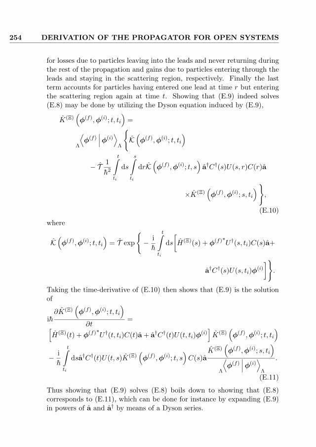
254 DERIVATION OF THE PROPAGATOR FOR OPEN SYSTEMS
for losses due to particles leaving into the leads and never returning duringthe rest of the propagation and gains due to particles entering through theleads and staying in the scattering region, respectively. Finally the lastterm accounts for particles having entered one lead at time r but enteringthe scattering region again at time t. Showing that (E.9) indeed solves(E.8) may be done by utilizing the Dyson equation induced by (E.9),
K(Ξ)(φ(f),φ(i); t, ti
)=⟨
φ(f)∣∣∣φ(i)
⟩Λ Λ
K(φ(f),φ(i); t, ti
)
− T 1
h2
t∫ti
ds
s∫ti
drK(φ(f),φ(i); t, s
)a†C†(s)U(s, r)C(r)a
×K(Ξ)(φ(f),φ(i); s, ti
),
(E.10)
where
K(φ(f),φ(i); t, ti
)= T exp
− i
h
t∫ti
ds
[H(Ξ)(s) + φ(f)∗U †(s, ti)C(s)a+
a†C†(s)U(s, ti)φ(i)
].
Taking the time-derivative of (E.10) then shows that (E.9) is the solutionof
ih∂K(Ξ)
(φ(f),φ(i); t, ti
)∂t
=[H(Ξ)(t) + φ(f)∗U †(t, ti)C(t)a + a†C†(t)U(t, ti)φ
(i)]K(Ξ)
(φ(f),φ(i); t, ti
)− i
h
t∫ti
dsa†C†(t)U(t, s)K(Ξ)(φ(f),φ(i); t, s
)C(s)a
K(Ξ)(φ(f),φ(i); s, ti
)⟨φ(f)
∣∣∣φ(i)⟩
Λ Λ
.
(E.11)
Thus showing that (E.9) solves (E.8) boils down to showing that (E.8)corresponds to (E.11), which can be done for instance by expanding (E.9)in powers of a and a† by means of a Dyson series.

E.3. STATIONARY PHASE APPROXIMATION 255
Thus, the propagator of the complete system with the leads projectedto coherent states one finally is indeed given by (E.1).
E.3 Getting real actions and stationary phaseapproximation
Starting from the path-integral representation (E.3) and projecting theleads to quadratures as well, using the overlap
〈φ|Q〉 =1√b√
2πexp
[−|φ|
2
2−(
Q
2b− φ∗
)2
+(φ∗)2
2
]. (E.12)
Therefore, the propagator with the leads also given in quadrature repre-sentation reads
K(q(f),q(i); Q(2),Q(1); t, ti
)=
∫d2LΛφ(f)
πLΛ
∫d2LΛφ(i)
πLΛ
exp
(−∣∣∣φ(f)
∣∣∣2 − ∣∣∣φ(i)∣∣∣2 + φ(f)∗U (t, ti)φ
(i)
)(√
2πb)LΛ
exp
−(Q(2)
2b− φ(f)
)2
+φ(f)2
2−(
Q(1)
2b− φ(i)d
)2
+φ(i)d
2
2
limN→∞
∫dLq(1) · · ·
∫dLq(N−1)
∫dLp(1)
(4πb2)L· · ·∫
dLp(N)
(4πb2)L
exp
iτ
4b2h
N∑k=1
[2hp(k)
(q(k) − q(k−1)
)τ
−H(Ξ)(ψ(k); tk
)−2bφ(f)dU(t, tk)C(tk)ψ
(k) − 2bψ(k)†C†(tk)U(tk, ti)φ(i)
+iτ
h
k−1∑l=1
ψ(k)†C†(ti + kτ)U(tk, tl)C(ti + lτ)ψ(l)
](E.13)

256 DERIVATION OF THE PROPAGATOR FOR OPEN SYSTEMS
yields after performing the integrations
K(q(f),q(i); Q(2),Q(1); t, ti
)=
exp
− i
4b2
(Q(1)
Q(2)
)(U (i)U (r) −U (i)
−U (i)TU (r)U (i)
)(Q(1)
Q(2)
)det√
2πb2 (1− UT (t, ti)U (t, ti))
× limN→∞
∫dLq(1) · · ·
∫dLq(N−1)
∫dLp(1)
(4πb2)L· · ·∫
dLp(N)
(4πb2)L
exp
iτ
4b2h
N∑k=1
[2hp(k)
(q(k) − q(k−1)
)τ
−H(Ξ)(ψ(k); tk
)+ 2Q(2)U (i)T=
[U †(tk, ti)C(tk)ψ
(k)]− 2Q(1)U (i)=
[U(t, tk)C(tk)ψ
(k)]
+2τ
h=[ψ(k)∗C†(tk)U
†(t, tk)]U (i)T
k−1∑l=1
=[U †(tl, ti)C(tl)ψ
(l)]]
,
(E.14)
where U (r) = < [U(t, ti)] and U (i) = = [U(t, ti)]. The second line is againthe free propagator of the isolated leads. Note that terms which will vanishin the limit N →∞ are already neglected.
Evaluatig the path integral in stationary phase approximation yields

E.3. STATIONARY PHASE APPROXIMATION 257
the equations of motion
0 =2h
τ
(p(k) − p(k+1)
)−∂H(Ξ)
(ψ(k); tk
)∂q(k−1)
+ 2=[CT(tk)U
∗(tk, ti)]U (i)Q(2)
− 2=[CT(tk)U
T(tf , tk)]U (i)T
Q(1)
+τ
h<[CT(tk)U
∗(tk, ti)U(i)
N∑l=1
U(tf , tl)C(tl)ψ(l)
]
− τ
h<[C†(tk)U
†(tf , tk)U(i)T
k−1∑l=1
U †(tl, ti)C(tl)ψ(l)
]
− τ
h<[CT(tk)U
∗(tk, ti)U(i)
N∑l=k+1
U∗(tf , tl)C∗(tl)ψ
(l)
]
(E.15)
0 =2h
τ
(q(k) − q(k−1)
)−∂H(Ξ)
(ψ(k); tk
)∂p(k−1)
+ 2=[iCT(tk)U
∗(tk, ti)]U (i)Q(2)
− 2=[iCT(tk)U
T(tf , tk)]U (i)T
Q(1)
+τ
h<[
iCT(tk)U∗(tk, ti)U
(i)N∑l=1
U(tf , tl)C(tl)ψ(l)
]
+τ
h<[
iC†(tk)U†(tf , tk)U
(i)Tk−1∑l=1
U †(tl, ti)C(tl)ψ(l)
]
− τ
h<[
iCT(tk)U∗(tk, ti)U
(i)N∑
l=k+1
U∗(tf , tl)C∗(tl)ψ
(l)
]
(E.16)
Recognizing that i= (ia)+= (a) = i< (a)+= (a) = ia∗, i< (ia)+< (a) =−i= (a) + <(a) = a∗, i= (ia)−= (a) = ia and i< (ia)−< (a) = −a, as wellas defining ψ(k) =
(q(k) + ip(k)
)/(2b), the equations of motion can after

258 DERIVATION OF THE PROPAGATOR FOR OPEN SYSTEMS
taking the limit N →∞ be written as
ihψ(s) =
∂H(Ξ) (ψ(s); s)
∂ψ∗(s)+
i
hC†(s)U(s, ti)U
(i)
tf∫ti
dr= [U(tf , r)C(r)ψ(r)]
− i
2bC†(s)U(s, ti)U
(i)Q(2) +i
2bC†(s)U †(tf , s)U
(i)TQ(1)
− i
hC†(s)
s∫ti
drU(s, r)C(r)ψ(r).
(E.17)

APPENDIX FLoop contributions
In this appendix, the derivation of the loop contributions will be brieflyreviewed following mostly references [32, 33, 37, 250, 252, 253] and adoptedto the van-Vleck propagator in Fock space. It will also be illustrated, howthe effective Planck’s constant 1/N enters these contributions.
These contributions arise from trajectories, which at some time comeclose to themselves or their time reverse. The region in phase space, wherethis happens is called encounter region, while the remaining parts of the
encounters
(encounter-)
stretches
Figure F.1: A trajectory pair consisting of one two- and one three-encounter. The encounter regions are marked by dashed circles. The re-maining parts of the trajectory pair are called “links”.
259
260 LOOP CONTRIBUTIONS
trajectories are called links (see also Fig. F.1). Their partner trajectoriesfollow them or their time reverse outside the encounter regions. In sucha region, a trajectory and its partner trajectory connect different links.These encounter contributions are also called loop contributions, since ifa link starts and ends at the same encounter, the trajectory looks like aloop. However, note that the loops are never closed in phase space, sincea trajectory can not cross itself in phase space. For later reference, theparts of the trajectory lying inside the encounter region will be denoted as(encounter-) stretches. Later on it will be discussed in more detail, how todefine the borders of an encounter region.
Before starting, there are two comments, which should be noted. First,the trajectories may differ in several such encounter regions, and second,due to the abstract way of presentation, without further discussing thenature of the time reversal operation, the derivations presented here arevalid for all symmetry classes GUE, GOE and GSE.
The discussion will start with two-leg-loops, since one-leg-loops can beconsidered as two-leg-loops, for which the encounter region is shifted to thestart or end of the trajectory.
F.1 Two-leg-loops
F.1.1 Phase-space geometry
First of all consider the trajectory γ and label its links in the order oftraversal, such that the stretch, in which γ starts is the first one, while theone where it ends is the (O+1)-th stretch, where O+1 is the total numberof links.
For this trajectory, define the phase space coordinates
x = (J,θ) (F.1)
with Jj = |ψj |2, θj = arg (ψj).The next step would be placing a Poincare surface of section (PSS) P
orthogonal to γ at an arbitrary phase space point xα,1 of the trajectorywithin each encounter region separating the links [32, 33]. Here, α labelsthe encounter, while the subscript 1 indicates that it is placed along thefirst traversal of the encounter region.
However, here not only the total energy but also the number of particlesis conserved, which leads to the integrability of the 2-site Bose-Hubbard

F.1. TWO-LEG-LOOPS 261
model and the fact that the trajectory γ lives on a 2L − 2-dimensionalmanifold within the phase space, rather than a 2L − 1-dimensional one.Therefore, P would be a 2L − 3-dimensional manifold, which means thatthere are not as many stable as unstable directions. In the derivation ofthe loop contributions, however, it is important that the number of stableand unstable manifolds are the same.
Thus, one also has to take advantage of the gauge invariance of ψ,i.e. the fact that, if ψ(t) is a solution of the equations of motion, thenψ = eiφψ is also a solution. This implies that the only information of thephases of the trajectory one needs, are the differences between the phases.Thus, the reduced phase space coordinates can be defined by
x =
(J1
N, . . . ,
JLN, θ2 − θ1, . . . , θL − θ1
), (F.2)
which then can be used to define the reduced Poincare surface of section(RPSS) Pr, which in turn is then 2L−4 dimensional with L−2 stable andunstable directions. Note that the amplitudes of ψ have also been devidedby the total number of particles, in order to have the effective Planck’sconstant heff = 1/N appearing explicitly in the expression of the actiondifference later on.
It should be noted that the idea to use constants of motion in order tofurther reduce the dimensionality of a Poincare surface of section is not anew one [300]. Furthermore, the definition of the phase space variables interms of phase differences rather than absolute phases corresponds to anadditional projection of the Poincare surface of section, such as has beenfrequently used in order to visualize them [300–311].
Within each encounter α, such a RPSS is then placed at an arbitraryphase space point xα,1 of γ perpendicular to the trajectory and will be
denoted as P(α)r . The time, at which the trajectory pierces through the
α-th RPSS for the first time will be denoted as tα,1. The trajectory then
pierces again through P(α)r at times tα,j at the phase space point xα,j ,
where the sequential index j runs from 2 to oα, which is the number oftraversals of the α-th encounter. An encounter will be denoted accordingto the number of its traversal as oα-encounter.
Next, depending on whether xα,j or T xα,j is close to xα,1, where Tdenotes the classical time reversal operation, the (small) phase space dif-ferences xα,j −xα,1 or T xα,j −xα,1 is decomposed into stable and unstable
262 LOOP CONTRIBUTIONS
directions,
(T )xα,j − xα,1 =
L−2∑l=1
(s
(α,j)l esl + u
(α,j)l eul
), (F.3)
where (T )xα,1 is either x, if the stretches are traversed in the same direc-tion, or T x else. The vectors esl and eul are the unit vectors along the stableand unstable directions and satisfy
eul ∧ esl = eul ·(
0 1−1 0
)esl = 1 (F.4)
Now the encounter regions can be defined more precisely. As already stated,each RPSS has to be placed within the corresponding encounter region.Furthermore, the phase space differences (F.3) have to be small, i.e. thestable and unstable coordinates have to satisfy,∣∣∣s(α,j)
l
∣∣∣ , ∣∣∣u(α,j)l
∣∣∣ < c. (F.5)
Here c is an arbitrary constant, which is small enough to allow linearizationof the motion, but still large compared to the effective Planck’s constant1/N . The borders of the encounter region are then defined such that thephase space separations of all stretches are smaller than this classical con-stant.
Due to exponential behavior of stable and unstable coordinates, thetime the trajectory needs from entering the α-th encounter region to pierc-
ing through P(α)r for the first time is approximately given by
t(α)s ∼ 1
λminl,j
lnc∣∣∣s(α,j)l
∣∣∣ , (F.6)
with λ being the largest Lyapunov exponent. Likewise the time, the tra-jectory spends inside the encounter after traversing xα,1 is estimated by
t(α)u ∼ 1
λminl,j
lnc∣∣∣u(α,j)l
∣∣∣ . (F.7)
Note that in Eqns. (F.6) and (F.7) as well as in the following, the minimumis taken with respect to both the dimensional and the sequential indexesl ∈ 1, . . . , L− 2 and j ∈ 2, . . . , oα.

F.1. TWO-LEG-LOOPS 263
The total time the trajectory needs in order to traverse the α-th en-counter, which is also called the encounter time, is given by the sum ofthese two times,
t(α)enc = t(α)
s + t(α)u . (F.8)
F.1.2 Partner trajectory
Let’s now turn towards the partner trajectory γ′, which pierces through
P(α)r at time tα,j in the reduced phase space point x′α,j . Its j-th stretch
switches within the encounter from following the (time reverse of the) k-thto the (time reverse of the) k′-th stretch of γ.
The differences between the piercing points of the partner trajectory
can be decomposed again into stable and unstable coordinates s(α,j)′k , u
(α,j)′k
according to (F.3). Since the stable (unstable) coordinates deviate expo-nentially when evolving the trajectory backward (forward) in time, thestable and unstable coordinates have to satisfy the relations
s(α,j)′ =s(α,k) (F.9)
u(α,j)′ =u(α,k′). (F.10)
F.1.3 Existence
The proof of the existence of the loops for the mean field dynamicsfollows exactly the same lines as for first quantized systems in Ref. [35],except that the phase space points have to be replaced by the reducedones, (F.2). The proof starts with periodic orbits, for which the existenceis shown by linearizing the motion along each loop of γ′ around γ.
The linearized motion relates the difference x′α,j −xα,k(j) with x′α,j−1−xα,k′(j−1), if the j-th link of γ′ follows γ, while it establishes a connectionbetween x′α,j−T xα,k(j) and x′α,j−1−T xα,k′(j−1), if the j-th link of γ′ followsT γ. Here, k(j) denotes the stretch of γ, along which the j-th stretch of γ′
enters the encounter, while k′(j) is the one along which it exits.This yields a set of O linear equations, which uniquely define the O
phase space coordinates of the partner trajectory γ′ as functions of thephase space coordinates of γ. The solution to these equations is given byEqns. (F.9,F.10) [33].
Finally, note that it turns out that the links have to be non-vanishing,which will be of importance later on.

264 LOOP CONTRIBUTIONS
PSS
x1
x1'
x2
x3
x2'
x3'
PSSk=1
j=1
k=2
j=3
j=2
k=3
Figure F.2: Periodic orbit with a three-encounter. In this example, thefirst stretch of the partner trajectory γ′ connects the first with second oneof γ, the second stretch of γ′ switches from the first to the third one of γand the third stretch of γ′ enters along the time reverse of the second oneof γ and exits along its third one.
Figure F.3: Creation of a three- (top) and four-encounter (bottom) byreconnecting the initially parallel stretches.
In order to translate the loop contributions to non-periodic orbits, theset of trajectories is assumed to arise from cutting a periodic one intoseveral pieces and using the same argumentation as sketched above.
F.1.4 Action difference
Apart from the encounter regions the links of the trajectory pairs closelyfollow each other yielding a vanishing (in the limit heff → 0) action differ-ence. The only non-vanishing action differences occur in the encounterregions. The total action difference is thus the sum over the action differ-ences of each encounter. Therefore, in this section, it is sufficient to onlyconsider the case of one single o-encounter.

F.1. TWO-LEG-LOOPS 265
In order to compute the action difference of such an encounter, it is bestto start from the diagonal case, where the j-th stretch of γ′ just follows thej-th stretch of γ and successively reconnecting entrances and exits of γ byγ′. Examples of how to generate a 3 and 4-encounter by these reconnectionsis shown in Fig. F.3 By transforming from the phase space coordinates
s(j)k , u
(j)k to s
(j)k , u
(j)k , which are the stable and unstable coordinates after
the j-th reconnection, the action difference can be written as a sum overaction differences of two-encounters [33],
∆R(o) =o−1∑j=1
∆R(2)j , (F.11)
where ∆R(2)j is the action difference of the 2-encounter corresponding to
the j-th reconnection. Note that this coordinate transformation is linearand volume preserving [33].
Therefore, it is enough to consider the action difference ∆R(2) of a two-encounter. Since the energies are the same for both trajectories, the actiondifference between the first stretch of γ to x1 and γ′ to x′1 is given by thecontour integral
∆R1 = h
x1∫x′1
dJ · θ.
When choosing the contour of the integration to lie in the RPSS, the un-stable directions can be chosen such that the contour coincides with one ofthe stable directions.
Repeating the same reasoning for the remaining parts of the encounter,gives the action difference as a contour integral over a closed loop, ∆R(2) =h∮
dJ · θ along a parallelogram x′1 → x1 → (T )x′2 → (T )x2 → x′1,spanned by x′1 − x1 = ueu and T x′2 − x1 = ses. Note that here thestable and unstable directions are chosen such that only one stable andunstable component of the expansion (F.3) is non-zero. Thus, due to nor-malization, Eq. (F.4), the action difference of a 2-encounter is given by∆R(2) = hNueu ∧ ses = hNsu, which can be formulated independent ofthe choice of the stable and unstable directions as ∆R(2) = hNs · u. Theadditional factor given by the total number of particles arises due to thedefinition of the reduced phase space coordinates (F.2).
Finally, the action difference of an o-encounter is given by
∆R(o) = hN∑j,k
s(j)k u
(j)k .

266 LOOP CONTRIBUTIONS
Note that the action difference is independent of the position of the RPSS[32]. Furthermore, it can be shown that the Maslov indices of the involvedtrajectories are equal [38].
F.1.5 Density of encounters
As already indicated in section F.1.3, the above considerations alsoinclude a whole series of encounters. Therefore, it is convenient to define avector v whose components vo are the number of o-encounters. The totalnumber of encounters can thus be written as Nenc =
∑o vo. Moreover,
O =∑
o ovo is the total number of encounter stretches.
Note that in the case of several encounters, there is one RPSS P(α)r
for each encounter α = 1, . . . , Nenc, which is traversed by γ at times tα,j ,j = 1, . . . , oα and the α-th encounter is characterized by (L − 2)(oα − 1)
stable and unstable coordinates s(α,j)l , u
(α,j)l , l = 1, . . . , L−2, j = 2, . . . , oα.
In the following, the derivation of the density w(2ll)T (s,u) of phase-space
separations s,u for two-leg-loop trajectories with evolution time T will beadopted to the case at hand. Here,
s =(s(1,2), . . . , s(Nenc,oNenc )
)is the vector containing all stable coordinates. Likewise u is the vectorcontaining all unstable coordinates. To make sure that each encounter iscounted exactly once, one has to demand that
c∫−c
d(L−2)(O−Nenc)sd(L−2)(O−Nenc)uw(2ll)T (s,u)
×∏α,j
δ(
∆Rα − hNs(α,j) · u(α,j))
yields the density of encounters sets in a trajectory γ leading to trajectorypairs (γ, γ′) with a given structure and an action difference of the α-thencounter given by ∆Rα.
w(2ll)T (s,u) should be understood as a quantity averaged over the ensem-
ble of all trajectories γ with duration T and weighted by the semiclassicalamplitude |Aγ |2.
Now assume that every RPSS and all times tα,1 are fixed. Due to
ergodicity, the probability of piercing through P(α)r again in a time interval

F.1. TWO-LEG-LOOPS 267
[tα,j , tα,j + dtα,j ] with stable and unstable coordinates in the set
L−2⊗l=1
([s
(α,j)l , s
(α,j)l + ds
(α,j)l ]⊗ [u
(α,j)l , u
(α,j)l + du
(α,j)l ]
)is given by dL−2s(α,j)dL−2u(α,j)dtα,j/ΩN (Eγ), where
ΩN (E) =
∫d2Lψδ (θ1) δ
(N −
L∑l=1
|ψl|2 +L
2
)δ [H (ψ∗,ψ)− E]
is the reduced phase space volume and Eγ is the energy of the trajectoryγ. Since the overall transformation (s, u) → (s,u) is volume preserving,the same uniform probability holds for (s,u).
Therefore the number
ρT (s,u, t)d(L−2)(O−Nenc)sd(L−2)(O−Nenc)udO−Nenct
of sets of O−Nenc piercings through the sections Pα, α = 1, . . . , Nenc occur-ing in time intervals [tα,j , tα,j + dtα,j ] with stable and unstable coordinatesin the set
L−2⊗k=1
([s
(α,j)k , s
(α,j)k + ds
(α,j)k ]⊗ [u
(α,j)k , u
(α,j)k + du
(α,j)k ]
)can be determined. However, one has to keep in mind that the links shallnot vanish. Therefore, a suitable characteristic function ΘT (s,u, t) has tobe employed, which is equal to 1 for non-vanishing links, and 0 otherwise.Thus
ρT (s,u, t) =ΘT (s,u, t)
ΩO−Nenc .
Finally, the density of phase space separations is given by integrating overthe piercing times tα,j , j = 2, . . . , oα, as well as over the positions of thereduced Poincare sections. However, this integration counts each encounter
for a time t(α)enc, such that w
(2ll)T (s,u) has to be devided by this time,
w(2ll)T (s,u) =
1
ΩO−NencN
∏αt(α)enc
∫dOtΘ(s,u, t). (F.12)
By substituting tj = tj + tj−1, the characteristic function Θ (s,u, t) yieldsthe integration limits 0 < t1 < . . . < tO < T −∑α oαt
αenc and w2ll
T (s,u) is
268 LOOP CONTRIBUTIONS
given by
w2llT (s,u) =
1
ΩO−NencN
∏αtαenc
T−∑αoαt
(α)enc∫
0
dtO
tO∫0
dtO−1 · · ·t2∫
0
dt1
=
(T −∑αoαt
(α)enc)O
O! ΩO−NencN
∏αt(α)enc
.
(F.13)
Note that the last step, where the time integrals have been performed, canonly be done, if the contribution of the trajectory pair does not depend onthe propagation times explicitly.
With this, the average number PvT (∆R)d∆R of partners differing from γ
in vl l-encounters, with an action difference in the interval [∆R,∆R+d∆R]can be determined. In order to take into account all possibilities, one hasto sum over all structures related to v and integrate over all phase-spaceseparations s,u leading to the same overall action difference ∆R = hNs ·u.One obtains
PvT,2ll(∆R)d∆R = d∆RN (v)
∫d(L−2)(O−Nenc)sd(L−2)(O−Nenc)u
δ(∆R− hNs · u)w(2ll)T (s,u),
where N (v) is the number of structures related to v.For a given trajectory γ, the sum over partner trajectories can finally
on disorder average be replaced according to∑γ′
. . .→∑v
∫d∆RPv
T,2ll(∆R) . . .
This replacement is possible, since the difference in the semiclassical am-plitudes Aγ and Aγ′ of the partner trajectories can be neglected.
F.2 One-leg-loops
For the discussion of one-leg-loops we will mainly Refs. [250, 252, 253].Since a one-leg-loop, which ends in an encounter gives the same contri-
bution as one which starts in an encounter, it is sufficient to consider only

F.2. ONE-LEG-LOOPS 269
the starting point to lie within an encounter region. The fact that bothcases give the same contribution can be seen very easily, by noticing thatthey are related by just exchanging s and u, which appear symmetricallyin the expressions for the action difference and the density of encounters.
In order to evaluate these contributions, consider a RPSS within thefirst encounter at time
t′ <1
λminl,j
lnc∣∣∣s(1,j)l
∣∣∣ ,
such that the encounter time is given by t(enc1) = t′ + tu. In order to
include every contribution, one has to integrate over all possible t′. Thusthe density of encounters has to be modified to be given by
w(1ll)T (s,u) =
1
ΩO−Nenc∏αt(α)enc
T−∑αoαt
(α)enc∫
0
dtO
tO∫0
dtO−1 · · ·t3∫
0
dt2
1λ
minj
(ln c
|sj|)
∫0
dt′.
(F.14)
Note that this does not include the case that both end points are veryclose to each other and therefore lie in the same encounter, i.e. coherentbackscattering contributions.
Apart from the changed density of encounters, which also brings alongdifferent dependencies on the stable and unstable coordinates, the furtherevaluation of one-leg-loops is the same as the one for two-leg-loops. Usually,it is reasonable to make a change of variables
t′′ = t′ +1
λminj
(ln
c
|uj |, uj =
c
σj, sj = cxjσj
),
with integration domains
−1 < xj < 1, 1 < σj < eλt′′, 0 < t′′ <
1
λminj
(ln
1
|xj |
),
in order to evaluate the resulting integrations over stable and unstablecoordinates.
When summing over all possible encounter structures with a one-leg-loop, one also has to account for the fact that each encounter stretch can

270 LOOP CONTRIBUTIONS
be chosen to contain the starting point of the trajectory. Therefore, anadditional sum over the number o1 of stretches of the first encounter hasto be inserted, where each term has to be weighted by the number vo1 ofsuch encounters. However, this sum is also included in the total number ofencounter structures, N (v). In order to compensate this double counting,one also has to divide by O, such that finally the number of partners for aone-leg-loop is given by
PvT,1ll(∆R)d∆R = d∆R
N (v)
O
∑o1
o1vo1
∫d(L−2)(O−Nenc)sd(L−2)(O−Nenc)u
δ(∆R− hNs · u)w(1ll)T (s,u).

APPENDIX GHubbard-Stratonovich
transformation
For the derivation of the van-Vleck propagator we will use a Hubbard-Stratonovich transformation in intermediate steps. Therefore we wouldlike to introduce it very briefly.
The Hubbard-Stratonovich transformation is based on Gaussian or Fres-nel integrals and it is used to decouple fourth-order terms in an exponential.Suppose we have an exponential eαyxyx where y and x do not neccessar-ily commute (later we will need the case that y is a creation and x anannihilation operator). This exponential can be written as
e−αyxyx =
∫dσe
βσ2+2β√αβσyx
∫dσeβσ2
,
which can be checked by shifting σ → σ −√α/βyx in the numerator:
∫dσe
βσ2+2β√αβσyx
=
∫dσe
β
(σ+√αβyx
)2
−αyxyx= e−αyxyx
∫dσeβσ
2.
Now lets have a look at what happens in higher dimensions. First weconsider the case that the exponent on the left hand side is of the form
271

272 HUBBARD-STRATONOVICH TRANSFORMATION
yαxαAαβyβxβ, where a sum over multiply occuring greek indices is implicit.Then the transformation is
e−αyηxηAηµyµxµ =
∫dσe
βσA−1σ+2β√αβσηyηxη
∫dσeβσA−1σ
,
where now σ is a vector and A−1 is the inverse of A, or more generally A−1
is defined by(A−1
)jαAαk = δjk, where δjk is the Kronecker delta. In this
case the shift σj → σj −√α/βAj,ηyηxη shows the identity of the left and
the right hand side.However this not yet includes the most general case of a fourth order
term, which would be xαxβAαβγδxγxδ. Here we will only consider thecase that A∗klmn = Amnkl and Aklmn = Alkmn = Aklnm. In this casethe integration no longer runs over (real or complex) numbers but over(hermitian) matrices and one possible form of the Hubbard Stratonovichtransformation in this case is
e−αyγxηAγδηµyδxµ =
∫dσe
βσδγ(A−1)γηδµ
σηµ+2β√αβσγδyγxδ
∫dσeβσδγ(A−1)γηδµσηµ
,
where(A−1
)klmn
is chosen such that(A−1
)kαlβ
Aαmβn = Aαkβl(A−1
)αmβn
= δkmδln.
To prove this case one has to shift σkl → σkl −√α/βAkγlδyγxδ.

Bibliography
273


Bibliography
[1] J. Franck and G. Hertz, Verh. Deut. Phys. Ges. 16, 457 (1914).
[2] N. Bohr, Phil. Mag. S. 6 26, 1 (1913).
[3] G. Tanner and K. Richter, Scholarpedia 8, 9818 (2013).
[4] E. Schrodinger, Phys. Rev. 28, 1049 (1926).
[5] C. Davisson, Bell System Tech. J. 7, 90 (1928).
[6] M. Brack and R. Bhaduri, Semiclassical Physics, 1st ed. (Westview Press,1997).
[7] J. H. Van Vleck, Proc. Natl. Acad. Sci. 14, 178 (1928).
[8] W. Pauli, Selected topics in field quantization, 1st ed. (MIT Press, 2000).
[9] R. P. Feynman, Rev. Mod. Phys. 20, 367 (1948).
[10] R. S. Whitney, Phys. Rev. B 75, 235404 (2007).
[11] M. C. Gutzwiller, J. Math. Phys. 8, 1979 (1967).
[12] L. S. Schulman, Techniques and applications of path integration (Wiley, NewYork, 1996).
[13] H. Kleinert, Path integrals in quantum mechanics, statistics, and polymerphysics, 3rd ed. (World Scientific, New Jersey, 2004).
[14] F. Haake, Quantum signatures of chaos, 3rd ed. (Springer, Berlin, 2010).
[15] M. C. Gutzwiller, Chaos in Classical and Quantum Mechanics (Springer,1990).
[16] M. C. Gutzwiller, J. Math. Phys. 12, 343 (1971).
[17] H. Weyl, Nachr. Ges. Wiss. Gott. math.-phys. Kl. 2, 110 (1911).
275

276 BIBLIOGRAPHY
[18] M. V. Berry, Proc. Roy. Soc. London. A. 400, 229 (1985).
[19] H. U. Baranger, R. A. Jalabert, and A. D. Stone, Phys. Rev. Lett. 70, 3876(1993).
[20] H. U. Baranger, R. A. Jalabert, and A. D. Stone, Chaos 3, 665 (1993).
[21] K. Richter and M. Sieber, Phys. Rev. Lett. 89, 206801 (2002).
[22] S. Hikami, A. I. Larkin, and Y. Nagaoka, Prog. Theor. Phys. 63, 707 (1980).
[23] O. Zaitsev, D. Frustaglia, and K. Richter, Phys. Rev. B 72, 155325 (2005).
[24] P. Jacquod and R. S. Whitney, Phys. Rev. B 73, 195115 (2006).
[25] R. A. Jalabert and H. M. Pastawski, Phys. Rev. Lett. 86, 2490 (2001).
[26] A. Goussev, R. A. Jalabert, H. M. Pastawski, and D. A. Wisniacki, Schol-arpedia 7, 11687 (2012).
[27] O. Bohigas, M. J. Giannoni, and C. Schmit, Phys. Rev. Lett. 52, 1 (1984).
[28] M. Sieber and K. Richter, Physica Scripta T90, 128 (2001).
[29] M. Turek, D. Spehner, S. Muller, and K. Richter, Phys. Rev. E 71, 016210(2005).
[30] S. Heusler, S. Muller, P. Braun, and F. Haake, J. Phys. A: Math. Gen. 37,L31 (2004).
[31] S. Muller, S. Heusler, P. Braun, F. Haake, and A. Altland, Phys. Rev. Lett.93, 014103 (2004).
[32] S. Muller, S. Heusler, P. Braun, F. Haake, and A. Altland, Phys. Rev. E72, 046207 (2005).
[33] S. Muller, Periodic-Orbit Approach to Universality in Quantum Chaos,Ph.D. thesis, Universitat Duisburg-Essen (2005).
[34] S. Heusler, S. Muller, P. Braun, and F. Haake, Phys. Rev. Lett. 96, 066804(2006).
[35] P. Braun, S. Heusler, S. Muller, and F. Haake, J. Phys. A: Math. Gen. 39,L159 (2006).
[36] T. Nagao, P. Braun, S. Muller, K. Saito, S. Heusler, and F. Haake,J. Phys. A: Math. Theor. 40, 47 (2007).
[37] S. Muller, S. Heusler, P. Braun, and F. Haake, New J. Phys. 9, 12 (2007).

BIBLIOGRAPHY 277
[38] M. Turek, Semiclassics beyond the diagonal approximation, Ph.D. thesis,Universitat Regensburg (2004).
[39] S. Muller, S. Heusler, A. Altland, P. Braun, and F. Haake, N. J. Phys. 11,103025 (2009).
[40] J. Kuipers, D. Waltner, C. Petitjean, G. Berkolaiko, and K. Richter, Phys.Rev. Lett. 104, 027001 (2010).
[41] J. Kuipers, T. Engl, G. Berkolaiko, C. Petitjean, D. Waltner, andK. Richter, Phys. Rev. B 83, 195316 (2011).
[42] P. A. Lee and A. D. Stone, Phys. Rev. Lett. 55, 1622 (1985).
[43] R. A. Jalabert, H. U. Baranger, and A. D. Stone, Phys. Rev. Lett. 65, 2442(1990).
[44] P. W. Brouwer and S. Rahav, Phys. Rev. B 74, 075322 (2006).
[45] A. Goussev, D. Waltner, K. Richter, and R. A. Jalabert, N. J. Phys. 10,093010 (2008).
[46] B. Gutkin, D. Waltner, M. Gutierrez, J. Kuipers, and K. Richter, Phys.Rev. E 81, 036222 (2010).
[47] R. S. Whitney and P. Jacquod, Phys. Rev. Lett. 103, 247002 (2009).
[48] P. Jacquod and R. S. Whitney, Europhys. Lett. 91, 67009 (2010).
[49] T. Engl, J. Kuipers, and K. Richter, Phys. Rev. B 83, 205414 (2011).
[50] T. Hartmann, J. Michl, C. Petitjean, T. Wellens, J.-D. Urbina, K. Richter,and P. Schlagheck, Ann. Phys. 327, 1998 (2012).
[51] G. Berkolaiko and J. Kuipers, N. J. Phys. 13, 063020 (2011).
[52] J. Kuipers and K. Richter, J. Phys. A: Math. Theor. 46, 055101 (2013).
[53] G. Berkolaiko and J. Kuipers, J. Math. Phys. 54, 112103 (2013).
[54] G. Berkolaiko and J. Kuipers, J. Math. Phys. 54, 123505 (2013).
[55] J. Kuipers, Q. Hummel, and K. Richter, Phys. Rev. Lett. 112, 070406(2014).
[56] E. Abrahams, 50 Years of Anderson Localization (World Scientific Publish-ing Company, 2010).
[57] P. Wolfle and D. Vollhardt, Int. J. Mod. Phys. B 24, 1526 (2010).
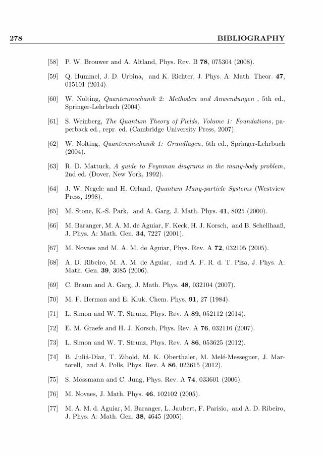
278 BIBLIOGRAPHY
[58] P. W. Brouwer and A. Altland, Phys. Rev. B 78, 075304 (2008).
[59] Q. Hummel, J. D. Urbina, and K. Richter, J. Phys. A: Math. Theor. 47,015101 (2014).
[60] W. Nolting, Quantenmechanik 2: Methoden und Anwendungen , 5th ed.,Springer-Lehrbuch (2004).
[61] S. Weinberg, The Quantum Theory of Fields, Volume 1: Foundations, pa-perback ed., repr. ed. (Cambridge University Press, 2007).
[62] W. Nolting, Quantenmechanik 1: Grundlagen, 6th ed., Springer-Lehrbuch(2004).
[63] R. D. Mattuck, A guide to Feynman diagrams in the many-body problem,2nd ed. (Dover, New York, 1992).
[64] J. W. Negele and H. Orland, Quantum Many-particle Systems (WestviewPress, 1998).
[65] M. Stone, K.-S. Park, and A. Garg, J. Math. Phys. 41, 8025 (2000).
[66] M. Baranger, M. A. M. de Aguiar, F. Keck, H. J. Korsch, and B. Schellhaaß,J. Phys. A: Math. Gen. 34, 7227 (2001).
[67] M. Novaes and M. A. M. de Aguiar, Phys. Rev. A 72, 032105 (2005).
[68] A. D. Ribeiro, M. A. M. de Aguiar, and A. F. R. d. T. Piza, J. Phys. A:Math. Gen. 39, 3085 (2006).
[69] C. Braun and A. Garg, J. Math. Phys. 48, 032104 (2007).
[70] M. F. Herman and E. Kluk, Chem. Phys. 91, 27 (1984).
[71] L. Simon and W. T. Strunz, Phys. Rev. A 89, 052112 (2014).
[72] E. M. Graefe and H. J. Korsch, Phys. Rev. A 76, 032116 (2007).
[73] L. Simon and W. T. Strunz, Phys. Rev. A 86, 053625 (2012).
[74] B. Julia-Dıaz, T. Zibold, M. K. Oberthaler, M. Mele-Messeguer, J. Mar-torell, and A. Polls, Phys. Rev. A 86, 023615 (2012).
[75] S. Mossmann and C. Jung, Phys. Rev. A 74, 033601 (2006).
[76] M. Novaes, J. Math. Phys. 46, 102102 (2005).
[77] M. A. M. d. Aguiar, M. Baranger, L. Jaubert, F. Parisio, and A. D. Ribeiro,J. Phys. A: Math. Gen. 38, 4645 (2005).

BIBLIOGRAPHY 279
[78] J. Bolte and S. Keppeler, Phys. Rev. Lett. 81, 1987 (1998).
[79] R. G. Littlejohn and W. G. Flynn, Phys. Rev. A 45, 7697 (1992).
[80] J. Bolte and R. Glaser, Ann. H. Poincare 6, 625 (2005).
[81] M. Pletyukhov, C. Amann, M. Mehta, and M. Brack, Phys. Rev. Lett. 89,116601 (2002).
[82] M. Pletyukhov and O. Zaitsev, J. Phys. A: Math. Gen. 36, 5181 (2003).
[83] M. Brack, C. Amann, M. Pletyukhov, and O. Zaitsev, Int. J. Mod. Phys. E13, 19 (2004).
[84] A. D. Ribeiro, M. A. M. de Aguiar, and A. F. R. de Toledo Piza, J. Math.Phys. 48, 112103 (2007).
[85] H.-D. Meyer and W. H. Miller, J. Chem. Phys. 71, 2156 (1979).
[86] W. H. Miller and K. A. White, J. Chem. Phys. 84, 5059 (1986).
[87] J. Kempe, Contemp. Phys. 44, 307 (2003).
[88] S. Godoy and S. Fujita, J. Chem. Phys 97, 5148 (1992).
[89] Y. Aharonov, L. Davidovich, and N. Zagury, Phys. Rev. A 48, 1687 (1993).
[90] E. Farhi and S. Gutmann, Phys. Rev. A 58, 915 (1998).
[91] H. B. Perets, Y. Lahini, F. Pozzi, M. Sorel, R. Morandotti, and Y. Silber-berg, Phys. Rev. Lett. 100, 170506 (2008).
[92] V. M. Kendon, Phil. Trans. R. Soc. A 364, 3407 (2006).
[93] E. Gerjuoy, Phys. Rev. A 67, 052308 (2003).
[94] R. P. Feynman and A. R. Hibbs, Quantum mechanics and path integrals(McGraw-Hill Companies, 1965).
[95] A. Schreiber, K. N. Cassemiro, V. Potocek, A. Gabris, P. J. Mosley, E. An-dersson, I. Jex, and C. Silberhorn, Phys. Rev. Lett. 104, 050502 (2010).
[96] A. Schreiber, A. Gabris, P. P. Rohde, K. Laiho, M. Stefanak, V. Potocek,C. Hamilton, I. Jex, and C. Silberhorn, Science 336, 55 (2012).
[97] A. Schreiber, K. N. Cassemiro, V. Potocek, A. Gabris, I. Jex, and C. Sil-berhorn, Phys. Rev. Lett. 106, 180403 (2011).
[98] C. K. Hong, Z. Y. Ou, and L. Mandel, Phys. Rev. Lett. 59, 2044 (1987).

280 BIBLIOGRAPHY
[99] A. Rai, G. S. Agarwal, and J. H. H. Perk, Phys. Rev. A 78, 042304 (2008).
[100] J. O. Owens, M. A. Broome, D. N. Biggerstaff, M. E. Goggin, A. Fedrizzi,T. Linjordet, M. Ams, G. D. Marshall, J. Twamley, M. J. Withford, andA. G. White, N. J. Phys. 13, 075003 (2011).
[101] O. Mulken and A. Blumen, Phys. Rep. 502, 37 (2011).
[102] D. N. Christodoulides, F. Lederer, and Y. Silberberg, Nature 424, 817(2003).
[103] A. Rai and D. G. Angelakis, Phys. Rev. A 85, 052330 (2012).
[104] B. C. Travaglione and G. J. Milburn, Phys. Rev. A 65, 032310 (2002).
[105] W. Dur, R. Raussendorf, V. M. Kendon, and H.-J. Briegel, Phys. Rev. A66, 052319 (2002).
[106] M. Karski, L. Frster, J.-M. Choi, A. Steffen, W. Alt, D. Meschede, andA. Widera, Science 325, 174 (2009).
[107] H. Schmitz, R. Matjeschk, C. Schneider, J. Glueckert, M. Enderlein, T. Hu-ber, and T. Schaetz, Phys. Rev. Lett. 103, 090504 (2009).
[108] F. Zahringer, G. Kirchmair, R. Gerritsma, E. Solano, R. Blatt, and C. F.Roos, Phys. Rev. Lett. 104, 100503 (2010).
[109] R. Grimm, M. Weidemuller, and Y. B. Ovchinnikov, Advances In Atomic,Molecular, and Optical Physics 42 (2000).
[110] O. Dutta, M. Gajda, P. Hauke, M. Lewenstein, D.-S. Luhmann, B. A. Mal-omed, T. Sowinski, and J. Zakrzewski, arXiv:1406.0181 (2014).
[111] M. Lewenstein, A. Sanpera Trigueros, and V. Ahufinger, Ultracold atomsin optical lattices : simulating quantum many-body systems, 1st ed. (Ox-ford Univ. Press, Oxford, 2012); M. Lewenstein, A. Sanpera, V. Ahufinger,B. Damski, A. Sen(De), and U. Sen, Adv. Phys. 56, 243 (2007).
[112] H. Feshbach, Ann. Phys. 5, 357 (1958).
[113] H. Feshbach, Ann. Phys. 19, 287 (1962).
[114] U. Fano, Phys. Rev. 124, 1866 (1961).
[115] See C. Chin, R. Grimm, P. Julienne, and E. Tiesinga, Rev. Mod. Phys. 82,1225 (2010) for a recent review of Feshbach resonances in ultra-cold atoms.
[116] S. Inouye, R. A. M., J. Stenger, H.-J. Miesner, M. S.-K. D., and W. Ketterle,Nature 392, 151 (1998).

BIBLIOGRAPHY 281
[117] P. Courteille, R. S. Freeland, D. J. Heinzen, F. A. van Abeelen, and B. J.Verhaar, Phys. Rev. Lett. 81, 69 (1998).
[118] N. F. Mott and R. Peierls, Proc. Phys. Soc. A 49, 72 (1937).
[119] N. F. Mott, Proc. Phys. Soc. A 62, 416 (1949).
[120] M. Greiner, O. Mandel, T. Esslinger, T. W. Hansch, and I. Bloch, Nature415, 39 (2002).
[121] D. Jaksch, C. Bruder, J. I. Cirac, C. W. Gardiner, and P. Zoller, Phys. Rev.Lett. 81, 3108 (1998).
[122] Y. Kurosaki, Y. Shimizu, K. Miyagawa, K. Kanoda, and G. Saito, Phys.Rev. Lett. 95, 177001 (2005).
[123] P. A. Lee, N. Nagaosa, and X.-G. Wen, Rev. Mod. Phys. 78, 17 (2006).
[124] P. A. Lee, Rep. Prog. Phys. 71, 012501 (2008).
[125] D. Jaksch and P. Zoller, Ann. Phys. 315, 52 (2005).
[126] T. Stoferle, H. Moritz, C. Schori, M. Kohl, and T. Esslinger, Phys. Rev.Lett. 92, 130403 (2004).
[127] S. Peil, J. V. Porto, B. L. Tolra, J. M. Obrecht, B. E. King, M. Subbotin,S. L. Rolston, and W. D. Phillips, Phys. Rev. A 67, 051603 (2003).
[128] W. S. Bakr, J. I. Gillen, A. Peng, S. Folling, and M. Greiner, Nature 462,74 (2009).
[129] J. Sherson, C. Weitenberg, M. Endres, M. Cheneau, I. Bloch, and S. Kuhr,Nature 467, 68 (2010).
[130] J. E. Lye, L. Fallani, M. Modugno, D. S. Wiersma, C. Fort, and M. Inguscio,Phys. Rev. Lett. 95, 070401 (2005).
[131] K. W. Madison, F. Chevy, W. Wohlleben, and J. Dalibard, Phys. Rev. Lett.84, 806 (2000).
[132] J. R. Abo-Shaeer, C. Raman, J. M. Vogels, and W. Ketterle, Science 292,476 (2001).
[133] V. Schweikhard, I. Coddington, P. Engels, V. P. Mogendorff, and E. A.Cornell, Phys. Rev. Lett. 92, 040404 (2004).
[134] Zwierlein M. W., Abo-Shaeer J. R., Schirotzek A., Schunck C. H., andKetterle W., Nature 435, 1047 (2005).

282 BIBLIOGRAPHY
[135] Y.-J. Lin, R. Compton, K. Jimenez-Garcıa, J. Porto, and I. Spielman,Nature 462, 628 (2009).
[136] L. Tarruell, D. Greif, T. Uehlinger, G. Jotzu, and T. Esslinger, Nature 483,302 (2012).
[137] Y.-J. Lin, K. Jimenez-Garcia, and I. B. Spielman, Nature 471, 83 (2011).
[138] J. D. Sau, R. Sensarma, S. Powell, I. B. Spielman, and S. Das Sarma, Phys.Rev. B 83, 140510 (2011).
[139] D. L. Campbell, G. Juzeliunas, and I. B. Spielman, Phys. Rev. A 84, 025602(2011).
[140] S. A. Wolf, D. D. Awschalom, R. A. Buhrman, J. M. Daughton, S. vonMolnar, M. L. Roukes, A. Y. Chtchelkanova, and D. M. Treger, Science294, 1488 (2001).
[141] I. Zutic, J. Fabian, and S. Das Sarma, Rev. Mod. Phys. 76, 323 (2004).
[142] S. Bader and S. Parkin, Ann. Rev. Cond. Mat. Phys. 1, 71 (2010).
[143] M. N. Baibich, J. M. Broto, A. Fert, F. N. Van Dau, F. Petroff, P. Etienne,G. Creuzet, A. Friederich, and J. Chazelas, Phys. Rev. Lett. 61, 2472 (1988).
[144] G. Binasch, P. Grunberg, F. Saurenbach, and W. Zinn, Phys. Rev. B 39,4828 (1989).
[145] M. Julliere, Phys. Lett. A 54, 225 (1975).
[146] D. Ralph and M. Stiles, J. Mag. Mag. Mat. 320, 1190 (2008).
[147] Y. A. Bychkov and E. I. Rashba, J. Phys. C: Solid State Phys. 17, 6039(1984).
[148] G. Dresselhaus, Phys. Rev. 100, 580 (1955).
[149] M. I. D’yakonov and V. I. Perel, Sov. Phys. JETP Lett. 13, 467 (1971);M. I. Dyakonov and V. I. Perel, Phys. Lett. A 35, 459 (1971).
[150] Y. K. Kato, R. C. Myers, A. C. Gossard, and D. D. Awschalom, Science306, 1910 (2004).
[151] C. L. Kane and E. J. Mele, Phys. Rev. Lett. 95, 226801 (2005).
[152] B. A. Bernevig and S.-C. Zhang, Phys. Rev. Lett. 96, 106802 (2006).
[153] M. Konig, S. Wiedmann, C. Brune, A. Roth, H. Buhmann, L. W.Molenkamp, X.-L. Qi, and S.-C. Zhang, Science 318, 766 (2007).

BIBLIOGRAPHY 283
[154] J. Maciejko, T. L. Hughes, and S.-C. Zhang, Ann. Rev. Cond. Mat. Phys.2, 31 (2011).
[155] S. Datta and B. Das, Appl. Phys. Lett. 56, 665 (1990).
[156] M. Wu, J. Jiang, and M. Weng, Phys. Rep. 493, 61 (2010).
[157] D. Averin and K. Likharev, Zh. Eksp. Teor. Fiz. 89, 733 (1986); D. Averinand K. Likharev, Sov. Phys. JETP 63, 427 (1986).
[158] L. S. Kuz’min and K. K. Likharev, Pis’ma Zh. Eksp. Teor. Fiz. 45, 389(1987); L. S. Kuz’min and K. K. Likharev, JETP Lett. 45, 495 (1987).
[159] T. A. Fulton and G. J. Dolan, Phys. Rev. Lett. 59, 109 (1987).
[160] K. Mullen, E. Ben-Jacob, R. C. Jaklevic, and Z. Schuss, Phys. Rev. B 37,98 (1988); M. Amman, K. Mullen, and E. BenJacob, J. Appl. Phys. 65,339 (1989).
[161] K. Likharev, IBM J. Res. Dev. 32, 144 (1988).
[162] L. I. Glazman and R. I. Shekhter, J. Phys.: Cond. Mat. 1, 5811 (1989).
[163] H. van Houten, C.W.J. Beenakker, and A.A.M. Staring, in Single ChargeTunneling: Coulomb Blockade Phenomena in Nanostructures, NATOAdv. Sci. Inst. Ser. B, Vol. 294, edited by H. Grabert and M. H. Grabert(WILEY-VCH Verlag GmbH, 1992); see also e-print H. van Houten, C. W. J.Beenakker, and A. A. M. Staring, arXiv:cond-mat/0508454 (2005).
[164] I. Giaever and H. R. Zeller, Phys. Rev. Lett. 20, 1504 (1968); H. R. Zellerand I. Giaever, Phys. Rev. 181, 789 (1969).
[165] D. V. Averin and Y. V. Nazarov, Phys. Rev. Lett. 65, 2446 (1990).
[166] D. Averin and Y. V. Nazarov, in Single Charge Tunneling: Coulomb Block-ade Phenomena in Nanostructures, NATO Adv. Sci. Inst. Ser. B, Vol. 294,edited by H. Grabert and M. H. Devoret (Plenum Press, 1992) p. 217.
[167] S. De Franceschi, S. Sasaki, J. M. Elzerman, W. G. van der Wiel, S. Tarucha,and L. P. Kouwenhoven, Phys. Rev. Lett. 86, 878 (2001).
[168] M. Pustilnik and L. Glazman, J. Phys.: Cond. Mat. 16, R513 (2004).
[169] J. Kondo, Prog. Theor. Phys. 32, 37 (1964).
[170] W. d. Haas, J. d. Boer, and G. v. d. Berg, Physica 1, 1115 (1934).

284 BIBLIOGRAPHY
[171] L. Kouwenhoven, C. Marcus, P. McEuen, S. Tarucha, R. Westervelt, andN. Wingreen, in Mesoscopic Electron Transport , NATO Adv. Sci. Inst. Ser.,Vol. 345, edited by L. Sohn, L. Kouwenhoven, and G. Schon (SpringerNetherlands, 1997) p. 105; M. A. Kastner, Rev. Mod. Phys. 64, 849 (1992).
[172] P. Joyez, V. Bouchiat, D. Esteve, C. Urbina, and M. H. Devoret, Phys.Rev. Lett. 79, 1349 (1997).
[173] Goldhaber-Gordon D., Shtrikman Hadas, Mahalu D., Abusch-MagderDavid, Meirav U., and Kastner M. A., Nature 391, 156 (1998).
[174] S. M. Cronenwett, T. H. Oosterkamp, and L. P. Kouwenhoven, Science 281,540 (1998).
[175] J. Schmid, J. Weis, K. Eberl, and K. v. Klitzing, Physica B: Cond. Mat.256–258, 182 (1998).
[176] S. Tarucha, D. G. Austing, Y. Tokura, W. G. van der Wiel, and L. P.Kouwenhoven, Phys. Rev. Lett. 84, 2485 (2000).
[177] L. P. Kouwenhoven, D. G. Austing, and S. Tarucha, Rep. Prog. Phys. 64,701 (2001).
[178] Sasaki S., De Franceschi S., Elzerman J. M., van der Wiel W. G., Eto M.,Tarucha S., and Kouwenhoven L. P., Nature 405, 764 (2000).
[179] M. Pustilnik, L. Glazman, D. Cobden, and L. Kouwenhoven, in InteractingElectrons in Nanostructures, Lecture Notes in Physics, Vol. 579, edited byR. Haug and H. Schoeller (Springer Berlin Heidelberg, 2001) pp. 3–24.
[180] J. Martinek, Y. Utsumi, H. Imamura, J. Barnas, S. Maekawa, J. Konig, andG. Schon, Phys. Rev. Lett. 91, 127203 (2003).
[181] J. Nygard, D. H. Cobden, and P. E. Lindelof, Nature 408, 342 (2000).
[182] W. Liang, M. Bockrath, and H. Park, Phys. Rev. Lett. 88, 126801 (2002).
[183] P. Jarillo-Herrero, J. Kong, H. S. van der Zant, C. Dekker, L. P. Kouwen-hoven, and S. De Franceschi, Nature 434, 484 (2005).
[184] L. Borda, G. Zarand, W. Hofstetter, B. I. Halperin, and J. von Delft, Phys.Rev. Lett. 90, 026602 (2003).
[185] M.-S. Choi, R. Lopez, and R. Aguado, Phys. Rev. Lett. 95, 067204 (2005).
[186] J. S. Lim, M.-S. Choi, M. Y. Choi, R. Lopez, and R. Aguado, Phys. Rev.B 74, 205119 (2006).

BIBLIOGRAPHY 285
[187] J. S. Lim, R. Lopez, G. L. Giorgi, and D. Sanchez, Phys. Rev. B 83, 155325(2011).
[188] D. R. Schmid, S. Smirnov, M. Marganska, A. Dirnaichner, P. L. Stiller,M. Grifoni, A. K. Huettel, and C. Strunk, (2013), arXiv:1312.6586 .
[189] M.-S. Choi, D. Sanchez, and R. Lopez, Phys. Rev. Lett. 92, 056601 (2004).
[190] I. Affleck, Nucl. Phys. B 336, 517 (1990).
[191] M. Fowler and A. Zawadowski, Solid State Commun. 9, 471 (1971).
[192] I. Affleck, Acta Phys. Pol. B 26, 1869 (1995).
[193] J. P. Bergfield, Z.-F. Liu, K. Burke, and C. A. Stafford, Phys. Rev. Lett.108, 066801 (2012).
[194] A. Rosch, J. Paaske, J. Kroha, and P. Wolfle, J. Phys. Soc. Jpn. 74, 118(2005).
[195] D. Roosen, M. R. Wegewijs, and W. Hofstetter, Phys. Rev. Lett. 100,087201 (2008).
[196] H. Schoeller and F. Reininghaus, Phys. Rev. B 80, 045117 (2009).
[197] M. A. Kastner, Phys. Today 46, 24 (1993).
[198] R. C. Ashoori, Nature 379, 413 (1996).
[199] B. Szafran, S. Bednarek, and J. Adamowski, Phys. Rev. B 67, 045311(2003).
[200] K. Jauregui, W. Husler, and B. Kramer, Europhys. Lett. 24, 581 (1993).
[201] S. Bednarek, T. Chwiej, J. Adamowski, and B. Szafran, Phys. Rev. B 67,205316 (2003).
[202] W. H. Miller, J. Chem. Phys. 53, 1949 (1970).
[203] W. H. Miller, Adv. Chem. Phys. 30, 77 (1975).
[204] E. J. Heller, J. Chem. Phys. 62, 1544 (1975).
[205] E. J. Heller, J. Chem. Phys. 75, 2923 (1981).
[206] M. J. Davis and E. J. Heller, J. Chem. Phys. 71, 3383 (1979).
[207] K. C. Kulander and E. J. Heller, J. Chem. Phys. 69, 2439 (1978).
[208] R. A. Marcus, Faraday Discuss. Chem. Soc. 55, 34 (1973).

286 BIBLIOGRAPHY
[209] W. H. Miller and T. F. George, J. Chem. Phys. 56, 5637 (1972).
[210] W. H. Miller, J. Chem. Phys. 68, 4431 (1978).
[211] W. H. Miller and C. W. McCurdy, J. Chem. Phys. 69, 5163 (1978).
[212] C. W. McCurdy, H. D. Meyer, and W. H. Miller, J. Chem. Phys. 70, 3177(1979).
[213] H.-D. Meyer and W. H. Miller, J. Chem. Phys. 70, 3214 (1979).
[214] W. H. Miller, Adv. Chem. Phys. 25, 69 (2007).
[215] M. Thoss and G. Stock, Phys. Rev. A 59, 64 (1999).
[216] B. Li and W. H. Miller, J. Chem. Phys. 137, 154107 (2012).
[217] D. W. H. Swenson, T. Levy, G. Cohen, E. Rabani, and W. H. Miller,J. Chem. Phys. 134, 164102 (2011).
[218] B. Li, W. H. Miller, T. J. Levy, and E. Rabani, J. Chem. Phys. 140, 204106(2014).
[219] B. Li, E. Y. Wilner, M. Thoss, E. Rabani, and W. H. Miller, J. Chem. Phys.140, 104110 (2014).
[220] J. D. Urbina, private communications.
[221] R. Shankar, Principles of quantum mechanics, 2nd ed. (Springer, New York,2008).
[222] P. A. M. Dirac, The principles of quantum mechanics, 4th ed., The interna-tional series of monographs on physics (Clarendon Press, Oxford, 1970).
[223] F. W. Byron and R. W. Fuller, Mathematics of classical and quantum physics: two volumes bound as one (Dover, London, 1992).
[224] H. F. Trotter, Proc. Amer. Math. Soc. 10, 545 (1959).
[225] M. Morse, The calculus of variations in the large, 5th ed. (American Math-ematical Society, Providence, 1966).
[226] E. W. Montroll, Communications on Pure and Applied Mathematics 5, 415(1952).
[227] F. Schwabl, Advanced Quantum Mechanics (Springer, 2008).
[228] W. Vogel and D.-G. Welsch, Quantum Optics, 3rd ed. (Wiley-VCH, 2006).
[229] I. Gradshteyn and I. Ryzhik, Table of Integrals Series and Products, 4th ed.(Academic, 1965).

BIBLIOGRAPHY 287
[230] F. Berezin, The Method of Second Quantization (Academic Press, 1966).
[231] J. R. Klauder, Ann. Phys. 11, 123 (1960).
[232] E. Akkermans and G. Montambaux, Mesoscopic Physics of Electrons andPhotons (Cambridge University Press, 2011).
[233] S. Datta, Electronic Transport in Mesoscopic Systems (Cambridge Univer-sity Press, 1997).
[234] A. J. Leggett, Rev. Mod. Phys. 73, 307 (2001).
[235] M. Pletyukhov, J. Math. Phys. 45, 1859 (2004).
[236] E. A. Kochetov, J. Math. Phys. 36, 4667 (1995).
[237] H. G. Solari, J. Math. Phys. 28, 1097 (1987).
[238] V. Vieira and P. Sacramento, Nucl. Phys. B 448, 331 (1995).
[239] T. Van Voorhis and E. J. Heller, Phys. Rev. A 66, 050501 (2002).
[240] T. Van Voorhis and E. J. Heller, J. Chem. Phys. 119, 12153 (2003).
[241] J. Kaidel, P. Winkler, and M. Brack, Phys. Rev. E 70, 066208 (2004).
[242] J. Kaidel, Extended semiclassical approximations for systems with mixedphase-space dynamics, Ph.D. thesis, Universitat Regensburg (2004).
[243] K. T. R. Davies, T. E. Huston, and M. Baranger, Chaos 2, 215 (1992).
[244] M. Brack, Foundations of Physics 31, 209 (2001).
[245] M. Brack, M. Mehta, and K. Tanaka, J. Phys. A: Math. Gen. 34, 8199(2001).
[246] P. Cvitanovic, R. Artuso, R. Mainieri, G. Tanner, and G. Vattay, Chaos:Classical and Quantum (Niels Bohr Institute, Copenhagen, 2012).
[247] W. H. Press, S. A. Teukolsky, W. T. Vetterling, and B. P. Flannery, Nu-merical Recipes, 3rd ed. (Cambridge University Press, 2007).
[248] J. Zinn-Justin, Path Integrals in Quantum Mechanics (Oxford UniversityPress, 2010).
[249] T. Engl, J. Dujardin, A. Arguelles, P. Schlagheck, K. Richter, and J. D.Urbina, Phys. Rev. Lett. 112, 140403 (2014).
[250] D. Waltner, Semiclassical Approach to Mesoscopic Systems, Springer Tractsin Modern Physics, Vol. 245 (Springer-Verlag, Berlin Heidelberg, 2012).

288 BIBLIOGRAPHY
[251] D. Waltner and K. Richter, “Classical Correlations and Quantum Inter-ference in Ballistic Conductors,” in Nonlinear Dynamics of Nanosystems(Wiley-VCH, 2010).
[252] D. Waltner, M. Gutierrez, A. Goussev, and K. Richter, Phys. Rev. Lett.101, 174101 (2008).
[253] M. Gutierrez, D. Waltner, J. Kuipers, and K. Richter, Phys. Rev. E 79,046212 (2009).
[254] J. Kuipers, D. Waltner, M. Gutierrez, and K. Richter, Nonlinearity 22,1945 (2009).
[255] M.-O. Mewes, M. R. Andrews, D. M. Kurn, D. S. Durfee, C. G. Townsend,and W. Ketterle, Phys. Rev. Lett. 78, 582 (1997).
[256] B. P. Anderson and M. A. Kasevich, Science 282, 1686 (1998).
[257] E. W. Hagley, L. Deng, M. Kozuma, J. Wen, K. Helmerson, S. L. Rolston,and W. D. Phillips, Science 283, 1706 (1999).
[258] I. Bloch, T. W. Hansch, and T. Esslinger, Phys. Rev. Lett. 82, 3008 (1999).
[259] G. Cennini, G. Ritt, C. Geckeler, and M. Weitz, Phys. Rev. Lett. 91, 240408(2003).
[260] N. P. Robins, C. Figl, S. A. Haine, A. K. Morrison, M. Jeppesen, J. J. Hope,and J. D. Close, Phys. Rev. Lett. 96, 140403 (2006).
[261] W. Guerin, J.-F. Riou, J. P. Gaebler, V. Josse, P. Bouyer, and A. Aspect,Phys. Rev. Lett. 97, 200402 (2006).
[262] J. Dujardin et al., “in preparation,” .
[263] J. Dujardin, A. Saenz, and P. Schlagheck, Appl. Phys. B , 1 (2014).
[264] A. Peres, Phys. Rev. A 30, 1610 (1984).
[265] N. Chernov, Scholarpedia 3, 4862 (2008).
[266] S. Trotzky, Y.-A. Chen, A. Flesch, I. McCulloch, U. Schollwock, J. Eisert,and I. Bloch, Nat. Phys. 8, 325 (2012).
[267] M. Gring, M. Kuhnert, T. Langen, T. Kitagawa, B. Rauer, M. Schreitl,I. Mazets, D. A. Smith, E. Demler, and J. Schmiedmayer, Science 337,1318 (2012).
[268] T. Langen, R. Geiger, M. Kuhnert, B. Rauer, and J. Schmiedmayer, Nat.Phys. 9, 640 (2013).

BIBLIOGRAPHY 289
[269] T. Geiger, T. Wellens, and A. Buchleitner, Phys. Rev. Lett. 109, 030601(2012).
[270] M. Abramowitz and I. Stegun, Handbook of mathematical functions (DoverPublications Inc., New York, 1970).
[271] J. D. Bodyfelt, M. Hiller, and T. Kottos, Europhys. Lett. 78, 50003 (2007).
[272] P. Schlagheck, private communications.
[273] M. L. Mehta, Random Matrices, 3rd ed. (Academic Press, 2004).
[274] Wikipedia, “Spin echo,” (2014), [Online; accessed 19-August-2014].
[275] E. L. Hahn, Phys. Rev. 80, 580 (1950).
[276] J. R. Klauder and P. W. Anderson, Phys. Rev. 125, 912 (1962).
[277] E. Abe, K. M. Itoh, J. Isoya, and S. Yamasaki, Phys. Rev. B 70, 033204(2004).
[278] B. Herzog and E. L. Hahn, Phys. Rev. 103, 148 (1956).
[279] W. M. Witzel, R. de Sousa, and S. Das Sarma, Phys. Rev. B 72, 161306(2005).
[280] X. X. Yi, H. Wang, and W. Wang, Eur. Phys. J. D 45, 355 (2007).
[281] W.-L. Ma, G. Wolfowicz, N. Zhao, S.-S. Li, J. J. L. Morton, and R.-B.Liu, “Uncovering many-body correlations in nanoscale nuclear spin bathsby central spin decoherence,” (2014), arXiv:1404.2717 .
[282] M. V. Berry and K. E. Mount, Rep. Prog. Phys. 35, 315 (1972).
[283] H.-J. Stockmann, Quantum Chaos: An Introduction (Cambridge UniversityPress, 1999).
[284] K. Richter, Semiclassical theory of mesoscopic quantum systems (Springer,Berlin, 2000).
[285] L. Wilets, E. Henley, M. Kraft, and A. Mackellar, Nucl. Phys. A 282, 341(1977).
[286] C. Dorso, S. Duarte, and J. Randrup, Phys. Lett. B 188, 287 (1987).
[287] D. H. Boal and J. N. Glosli, Phys. Rev. C 38, 1870 (1988).
[288] V. Latora, M. Belkacem, and A. Bonasera, Phys. Rev. Lett. 73, 1765 (1994).
[289] C. Gardiner and P. Zoller, Quantum Noise, 3rd ed. (Springer, Berlin, 2004).

290 BIBLIOGRAPHY
[290] A. Sinatra, C. Lobo, and Y. Castin, Phys. Rev. Lett. 87, 210404 (2001).
[291] D. Walls and G. J. Milburn, Quantum Optics (Springer, 2010).
[292] A. Polkovnikov, Ann. Phys. 325, 1790 (2010).
[293] D. A. Wisniacki, Phys. Rev. E 67, 016205 (2003).
[294] F. M. Cucchietti, H. M. Pastawski, and D. A. Wisniacki, Phys. Rev. E 65,045206 (2002).
[295] F. M. Cucchietti, H. M. Pastawski, and R. A. Jalabert, Phys. Rev. B 70,035311 (2004).
[296] C. Petitjean and P. Jacquod, Phys. Rev. E 71, 036223 (2005).
[297] M. Gutierrez and A. Goussev, Phys. Rev. E 79, 046211 (2009).
[298] J. Michl et al., private communications.
[299] S. Flach, (2014), arXiv:1405.1122 .
[300] L. Martinet and P. Magnenat, Astron. Astrophys. 96, 68 (1981).
[301] C. Froeschle, Astron. Astrophys. 4, 115 (1970).
[302] C. Froeschle, Astron. Astrophys. 16, 172 (1972).
[303] C. Froeschle and E. Lega, Celest. Mech. Dyn. Astron. 78, 167 (2000).
[304] S. Udry and D. Pfenniger, Astron. Astrophys. 198, 135 (1988).
[305] D. Pfenniger, Astron. Astrophys. 150, 97 (1985).
[306] C. Skokos, G. Contopoulos, and C. Polymilis, Celest. Mech. Dyn. Astron.65, 223 (1996).
[307] P. Magnenat, Celest. Mech. Dyn. Astron. 28, 319 (1982).
[308] M. N. Vrahatis, T. C. Bountis, and M. Kollmann, Int. J. Bif. Chaos 06,1425 (1996).
[309] P. A. Patsis and L. Zachilas, Int. J. Bif. Chaos 04, 1399 (1994).
[310] M. Katsanikas and P. A. Patsis, Int. J. Bif. Chaos 21, 467 (2011).
[311] M. Richter, S. Lange, A. Backer, and R. Ketzmerick, Phys. Rev. E 89,022902 (2014).


![Semiclassical theory [10pt] with self-generated magnetic field …weyl.math.toronto.edu/victor_ivrii_Publications/... · 2017-08-05 · Semiclassical theory with self-generated magnetic](https://img.pdfslide.net/doc/110x75/5e93f6de1f6ab1764979620f/semiclassical-theory-10pt-with-self-generated-magnetic-field-weylmath-2017-08-05.jpg)