THREE ESSAYS ON THE FACTOR CONTENT OF TRADE

THREE ESSAYS ON THE FACTOR CONTENT OF TRADE

A Dissertation

presented to

the Faculty of the Graduate School

University of Missouri-Columbia

In Partial Fulfillment

Of the Requirement for the Degree

Doctor of Philosophy

By

YEON JOON KIM

Dr. Vitor Trindade, Dissertation Supervisor

MAY 2009

© Copyright by Yeon Joon Kim 2009

All Rights Reserved

The undersigned, appointed by the dean of the Graduate School, have examined the

dissertation entitled


presented by Yeon Joon Kim,

a candidate for the degree of doctor of philosophy of Economics,

and hereby certify that, in their opinion, it is worthy of acceptance.

Professor Vitor Trindade

Professor Shawn Ni

Professor Gunjan Sharma

Professor X. H. Wang

Professor Cooper Drury

ii

ACKNOWLEDGEMENTS

I really appreciate Dr. Vitor Trindade, my dissertation advisor, for his guidance

through this dissertation and for his intellectual and precious guidance. I learned many

academic, professional, and personal things from him. Many thanks to my wonderful

committee members; Dr. Shawn Ni, Dr. Xinghe Wang, Dr. Gunjan Sharma, and Dr.

Cooper Drury gave me valuable discussions and encouragements. I appreciate Ms. Lynne

Riddell the graduate administrative assistant for her precious helps. I also appreciate Dr.

Inbong Kang, Steven Pleydle, Patty Buxton, Kyle Bosh, Dan Kowalski, and my best

friend Dr. Inkyu Kim, and all the members in the Ways and Means Committee, New

York State Assembly and all the members in the Legislative Research and Legislative

Budget Office, State of Missouri. I also appreciate the writing center of University of

Missouri.

My wholehearted appreciation should go to my family for their endless love and

support. More than anyone else, I would like to express my deepest and wholehearted

thanks to my wife, Yun Hee Kim for her love, sacrifice, and encouragements. I am also

thankful to my daughter Seo Yeon and son, Joel for their being with me. I dedicate this

dissertation to God.

iii

TABLE OF CONTENTS

ACKNOWLEDGMENTS .................................................................................................. ii

LIST OF TABLES ............................................................................................................. vi

LIST OF FIGURES ......................................................................................................... viii

ABSTRACT .................................................................................................................... ix

CHAPTERS

Chapter 1: Demand Effects in International Trade

I. Introduction ................................................................................................. 2

II. Theory and Empirical Methodology ............................................................7

II.1. Homothetic Preferences .......................................................................8

II.2. Non-homothetic Preferences ..............................................................11

III. Data ............................................................................................................17

IV. Empirical Analysis of Demand Effects ...................................................18

V. Conclusions ................................................................................................23

Chapter 2: The Relevance of Trade Costs for the Factor Content of Trade: A Comparison

of the Trans-Atlantic and the Intra-European Trade

I. Introduction ................................................................................................25

II. Literature Review ......................................................................................25

iv

III. Methodology and Models ..........................................................................35

IV. Empirical Tests ..........................................................................................41

V. Importance of Trade Costs and comparison of Trade Costs for Intra-

European Trade versus Other Trade ..........................................................45

VI. Test Results ................................................................................................50

VII. Concluding Remarks ................................................................................53

Chapter 3: Factor Content of Trade with Trade Costs

I. Introduction and Brief Overview of Existing Literature ............................57

II. Methodology and Models ..........................................................................67

II.1. Method 1……………………………………………………………67

II.2. Method 2……………………………………………………………71

III. Empirical Analysis……………………………………………………..73

IV. Concluding Remarks…………………………………………………….75

DATA APPENDIX

A. For Chapter One .........................................................................................77

A1. Output ..................................................................................................85

A2. Construction of the Matrix of Technical Coefficients ........................88

A3. Matrix of Direct Factor Inputs and Matrix of Total Factor Inputs ......90

A4. Final Demand, Trade, and Endowments .............................................94

v

A5. Generalization with Intermediate Inputs and Different Techniques ...97

B. For Chapter Three ....................................................................................100

B1. Data Sources………………………………………………………..100

B2. Countries…………………………………………………………...101

B3. Industries…………………………………………………………...101

B4. Trade Costs…………………………………………………………102

REFERENCES…………………………………………………………………………105

VITA ................................................................................................................................112

vi

LIST OF TABLES

Table Page

Chapter 1

1.1 Regression of Demand per capita on Income per capita……………………..18

1.2 Subsistence Consumptions…………………………………………………...20

1.3 Results based on hypotheses (H1) and (H2)…………………………………22

Chapter 2

2.1 Key Specification of Davis and Weinstein (2001a)……….………………....30

2.2 Trade Tests from Davis and Weinstein (2001a)……………………………..31

2.3 Country Groups for Test Equations 2-8 and 2-9……………………………..42

2.4 Specification of Models……………………………………………………...44

2.5 Trade Costs…………………………………………………………………..45

2.6 Tariff Rates, NTBs ratio, and Imports Duties………………………….……47

2.7 Bilateral Trade Costs (TC)………………………………………..…………49

vii

2.8 Bilateral Trade Costs…………………………………………………………50

2.9 Trade Test with Davis and Weinstein’s (2001a) Data, 1985………………...53

Chapter 3

3.1 Ad valorem Trade Costs by Two Digits SIC Industry and Year……….........63

3.2 Test Results of Trade Test…………………………………………………...74

DATA APPENDIX

A1. Countries with IO Tables……………………………………………..……..78

A2. List of Industries……………………………………………………….……80

A3. Format of the IO Data for Country c: No Data Incompleteness………….…82

A4. Format of the IO Data for country c: Some Incomplete Data ………………84

B1. Classification of Industrial Activities………………………………………101

B2. Trade Costs Rate (%)………………………………………………….…...103

viii

LIST OF FIGURES

Figure Page

Chapter 1

1.1 Income-expansion Path with Quasi-homothetic Preferences……………......12

Chapter 3

3.1 Average Manufacturing Industry Trade Costs over Time…………………...66

ix


YEON JOON KIM

Dr. Trindade Vitor, Dissertation Supervisor

ABSTRACT

This dissertation investigates the factor content of trade. This dissertation consists of

three chapters that explain the factor content of trade with different methodologies.

The first chapter is Demand Effects in International Trade. We supplement prevalent

international trade theory based on supply-side and extend the Heckscher-Ohlin-Vanek

model in a new direction by incorporating demand-side consideration. These have been

important in the “lore” of economics but not in economics research practice. We focus on

aggregate demand differences across different countries that are induced by inequality in

the presence of nonhomothetic preferences. We have constructed a new rich dataset that

has information on consumption, trade, and factor usage for 32 countries across 45

industries that span the whole economy, for a year circa 2000. We fit the data for

different types of preference assumptions, which allows us estimate preference

parameters. We then use these results, plus our new demand-side methodology, to

compare the relative importance of the supply-side and the demand-side in accounting for

global factor trade.

The second chapter, has the title the Relevance of Trade Costs for the Factor Content

of Trade: A Comparison of the Trans-Atlantic and the Intra-European Trade, extends the

original Heckscher-Ohlin-Vanek (HOV) model in a modified direction, with a

consideration of the pair-wise HOV model. Moreover, the original HOV model and the

pair-wise HOV model both assume that there are no trade costs. This chapter studies the

x

relevance of trade costs by comparing the fit of the factor content methodology for the

trans-Atlantic trade (that is, trade between the United States and several European

countries), and the purely intra-European trade (that is, trade among the largest five

European economies). This chapter also examines trade data that includes Australia and

Canada. Note by using the trans-Atlantic countries with Australia and Canada, this

chapter argues that the trans-Atlantic trade with Australia and Canada has higher trade

costs than the intra-European trade. The sign test performs well without major

amendments, but simply by restricting trade to the intra-European trade. The evidence

presented in this chapter is at least suggestive that trade costs may play a very significant

role in trade, and therefore in the calculation of the factor content of trade.

The third chapter is the Factor Content of Trade with Trade Costs. This chapter

expands upon the original HOV model by considering trade costs. It deduces the original

HOV model with trade costs and compares the importance of the original HOV model

with and without trade costs. It does so by including trade costs directly in the technology

matrix, where the working assumption is that the trade costs are located in the original

country. Additionally, this chapter includes trade costs directly in the vector of the net

exports. This chapter concludes that the original HOV model with trade costs achieves

better results than the model without trade costs using the data constructed for the

purpose of this chapter. These test results show that trade costs play an important role in

explaining the factor content of trade.

1

Chapter 1

Demand Effects in International Trade

2

I. Introduction

In a line of research that extends back to Vassily Leontieff's (1953) seminal study of

United States trade in factor services, economists have long been interested in using the

“factor content” methodology to test the factor proportions model of international trade.

This methodology requires calculating the amounts of each factor that are embodied in a

country’s trade and then comparing them to theoretically-derived predictions, which will

be based on the difference between the country’s endowments of each factor and the

average world endowment of the same factor. In the decades since Leontieff's work, this

line of research has threaded through many twists and turns, with spectacular failures

followed by no less spectacular successes. Starting with Leontieff's surprising failure to

demonstrate that the United States is a net exporter of capital services, the story runs

through Edward Leamer’s (1980) proof that the test proposed by Leontieff was the wrong

one and Leamer’s derivation of the theoretically correct test. However, even after

Leamer’s path breaking research, both Bowen, Leamer and Sveikauskas (1987) and

Daniel Trefler (1993) essentially confirmed Leontieff's findings. Importantly, Trefler

(1995) concluded that technological differences across different countries can add

predictive success to the empirics. Donald Davis and David Weinstein (2001a) amend the

standard multi-good factor proportions model of international trade model in various

ways, and argue that such an amended model can largely account for the observed factor

content of trade in a sample of developed countries.

Crucially, these recent successes all rely on “supply-side” models for the reasons why

countries trade. To see what we mean, and what a “demand-side” approach would look

like, note that a country’s aggregate exports of a good are trivially equal to its aggregate

3

supply minus its aggregate demand for that good. Therefore the casual observer of the

theory might expect to see some explanations for the structure of trade that are based on

the demand side, just as she observes some explanations that are based on the supply

side. This casual observer would be well-justified in forming her expectations. She would

also be remarkably wrong! In fact, there is a clear and strong bias in classical trade theory

towards supply-side explanations,1 a bias that naturally propagates into most empirical

application of trade theory.

There are at least three reasons to take demand considerations seriously, especially in

accounting for the structure of foreign trade in factor services. First, while the theoretical

preference for supply-side explanations may in fact reflect how the world works, we shall

never find out it unless if we test that explanation against appropriate alternatives. In

other words, even the negative result that the demand side does not matter (or does not

matter much) for international trade would be a useful result to have.

Second, even within the narrow confines of the factor proportions model, the only

way to sweep demand effects away is by assuming that tastes are homothetic, which

(with the added assumption that they are identical across different countries and different

people) is the only way to neutralize all demand-side determinants of trade. But the

assumption of homotheticity is empirically untenable. Even if we restrict ourselves to the

evidence provided by international trade studies, the list is already long: see, among

others, Thursby and Thursby (1987), Hunter and Markusen (1988), Hunter (1991),

Francois and Kaplan (1996) and Dalgin, Trindade and Mitra (2007), in all of which

1 It is important to mention the single most important exception: the work of Markusen (1986), who explicitly allows demand considerations as part of his “eclectic” explanations for the volume of trade. The adjective itself is revelatory of how much demand-side considerations have been absent from mainstream explanations of trade. A more recent contribution is Mitra and Trindade (2005).

4

homotheticity is rejected. For example, Hunter and Markusen (1988) show that income-

expansion paths intercept the axis for at least one of the goods (in consumption space)

significantly away from zero. This shows that people consume some goods before

consumption of other goods even starts, a violation of homotheticity. Furthermore, both

Francois and Kaplan (1996) and Dalgin et al. (2007) find that income distribution is a

strong indicator of trade flows, which would not happen if tastes were homothetic.

Hunter (1991) builds on Hunter and Markusen (1988) and concludes that “non-

homothetic preferences significantly contribute to trade flows. Approximately one quarter

of the volume of inter-industry trade flows is caused by non-homothetic preferences.”

The assumption of homotheticity is also rejected in by the consumption literature. In

the words of Deaton (1992, p. 9), “the supposition that there are neither luxuries nor

necessities contradicts both common sense and more than a hundred years of empirical

research.” Okubo (2008) uses the data in Ogaki and Reinhart (1998), and finds that the

latter’s assumption of homotheticity over durable and non-durable goods is strongly

rejected. Moving from consumption to financial literature, Aït-Sahalia, Parker and Yogo

(2004) find that using nonhomothetic preferences is useful in explaining the equity risk

premium puzzle. In particular, they take into account that stock holders are on average

richer than the general population and therefore their consumption patterns of luxuries are

much more responsive than those of necessities, as returns change.

Third, casual observation suggests that tastes may be quite different across different

cultures. It certainly does not seem the case, for example, that the Japanese have similar

consumption patterns as West Europeans of the same approximate income level. This

might for example explain why rice and tea may play a major role in Japan’s trade

5

(including the need to protect it), with coffee and wine playing that role in Europe’s

trade. In this way, then, differences in tastes as an explanation of trade flows are an

example of those stories that we tell to our undergraduates but that we fail to take

seriously as researchers.

In this chapter, we accept from the outset that consumer preferences may be non-

homothetic, and we rederive the factor content of trade under that assumption. In doing

so, we allow the data to actually dictate the best fit for preferences, and in particular we

allow for preferences to be homothetic. The methodology consists, in its essence, of

assuming a shape for consumers’ income-expansion paths, and deriving the theoretical

predictions for the factor content of trade based on that shape. This therefore imposes a

structure on the estimation. However, instead of simply assuming an income-expansion

path that is a straight line from the origin, as previous research assumes, we allow that

assumption to be relaxed.2 As a first step we begin by reproducing Davis and Weinstein’s

(2001a) first set of results under homothetic assumptions.3 In our second step, we assume

that tastes are non-homothetic, while keeping the assumption that they are identical

across countries.4 We estimate a system of equations similar to Hunter and Markusen’s

(1988) linear expenditure system for 32 countries and 45 industries around the year 2000,

after which we have enough information to calculate the predicted factor content of trade

and compare it with the actual factor content of trade of each country.

2 We point out that this is a simple (and in our opinion elegant) procedure. One common misperception is that since some demand-side theories are very simple, then no further work is needed. But that would be confusing simplicity with irrelevance! If the demand side is a major driving force of trade flows, surely we would like to measure its relative impact. 3 Differences in sample and methodolgy will prevent an exact replication of their results. 4 In this dissertation we restrict ourselves to quasi-homothetic tastes, which are defined by income-expansion paths that start on one of the axes at a point significantly different from zero, but that are straight lines thereafter. These are the same preferences assumed by Markusen (1986) and Hunter and Markusen (1988).

6

Our research is related to some recent work. Chung (2005) uses the factor content

methodology, and an assumption of nonhomothetic preferences, to address the specific

issue of what Trefler (1995) calls the missing trade. He uses country and factor-specific

factor consumption shares to estimate equations similar to Davis and Weinstein’s (2001a)

different specifications, and finds that nonhomothetic preferences do not contribute to an

explanation of the missing trade for total trade. However, he also tests hypotheses for

tradables only, and there he finds a large contribution of nonhomotheticity. A recent

important contribution is by Reimer and Hertel (2007), whose main interest is in an

explanation for the apparent missing trade. They adapt one test from Davis and Weinstein

(2001a) to the case of nonhomothetic tastes. However, they find that nonhomothetic

preferences do not contribute a major explanation for the missing trade. Contrasting with

our current approach, neither Chung (2007) nor Reimer and Hertel (2007) deduce the

testing equations directly. Rather they adopt testing equations from Davis and Weinstein

(2001a), changing them to reflect the nonhomothetic nature of preferences. We use a

different approach in this chapter, in that we deduce testing equations from first

principles. In a theoretical approach, Dinopoulos, Fujiwara and Shimomura (2007) argue

for the introduction of quasi-linear preferences in the study of international trade, and

find that the predicted factor content of trade with quasi-linear preferences is smaller than

the predicted factor content of trade with homothetic preferences if and only if the

numeraire good is capital intensive.

This chapter offers three main contributions. The first is largely methodological, in

that it provides a procedure to calculate correctly the factor content of trade in the

presence of more generalized preferences than previously assumed. The second

7

contribution consists of using the methodology for an assessment of the importance of

demand in trade. One last important contribution was the construction of a detailed data

set that we hope will be useful to other researchers. Based on data provided by the

Organization for Economic Cooperation and Development (OECD), the data set contains

32 countries, 45 industries, and two factors (labor and capital). For each country and

industry we have information about factor usage, production, value-added, and trade.

II. Theory and Empirical Methodology

Our discussion suggests that theoretically predicted factor content flows will vary

according to the assumptions made on preferences. To verify how much impact the

assumptions from the demand side matter, we follow a two step procedure. In the first

step, we create a benchmark by rederiving a model of the factor content that ignores all

demand-side effects. That is, we retread the basic model of Trefler (1995) and Davis and

Weinstein (2001a), based on Vanek’s (1968) model. The second step will relax

successive layers of assumptions on preferences, while in order to control for the supply

side we stay within the most simplistic version of the factor proportions model. Thus, we

assume throughout that preferences are identical across countries, all countries share

identical technologies, markets are competitive, there are no trade costs, all factors are

fully employed and all countries lie within the same “cone if diversification.”5 These

5 We emphasize that we do this to simplify the supply side of the analysis, and in order to isolate the possible demand-side effects. For example, see Schott (2003) for evidence that different countries may lie on multiple cones.

8

assumptions imply that techniques of production are identical and ensure factor price

equalization.

II.1. Homothetic Preferences

Let us assume that there are C countries, G goods and H factors of production.6 With

the standard assumptions of the factor proportions model as stated above, and with

homothetic preferences, each country’s consumption is proportional to world

consumption, with the proportion given by / , where Ic is country c’s

Gross Domestic Product (GDP), ∑ is the world’s GDP, and TBc is country c’s

trade balance. In words, sc is country c’s share of world income, corrected by the trade

balance to obtain its share of the world’s consumption. Writing the vectors of final

demand for country c and for the world as Dc and Dw, respectively, homotheticity implies

Dc Dw. Because world demand equals world supply, we can write equivalently:

Dc Yw, (1-1)

where Yw is the world vector of final world output. We write country c’s final goods

export vector as Tc Yc Dc, where Yc is country c’s final output vector (implying that

Yw ∑ Yc). We shall also use country c’s total factor input matrix, denoted by Bc. This

is distinguished from the direct factor input matrix (which we call Fc), in that Bc accounts

for all of the factors embodied in the production of a good, including those that are

embodied indirectly through intermediate inputs, through the intermediate inputs of the

intermediate inputs, and so on. We describe in the data section and in the data appendix

how we use input-output tables to construct a matrix Bc for each country c. 6 The letter F will be reserved for the factor content of trade.

9

We will then deduce a testing hypothesis that will be very similar to Trefler’s (1995)

test with Hicks-neutral productivity differences, and to Davis and Weinstein’s (2001a)

third hypothesis. Specifically, we assume that the matrices Bc for the several countries

differ in two ways only: all factors in country c are shifted by an “efficiency” factor ;

and matrix Bc may be measured with error. Thus, suppose that we have the elements

of matrix Bc, where the index c denotes the country, f denotes the factor, and i denotes the

industry. We then estimate the following equation:

ln , (1-2)

Equation (1-2) implies that , where and are parameters to be

estimated, and is the measurement error. This allows us to define exp as

the Hicks-neutral technology shift for country c. We choose the omitted dummy to be the

US’s, that is, we normalize the technology shift of the United States to be one. The larger

is, the higher the unit total factor requirements of the country are, and therefore the

lower the productivity of the country is. We interpret exp as the element of

the international reference matrix, denoted as B. The fitted elements for country c are

, and they form a matrix that we denote by Bc B . It has two parts: the

country’s technology factor , and the estimated international total factor input matrix B

(which is of course also the United States’ total factor input matrix).

We can also define the vector Vc whose element is country c’s endowment of

factor f. Given full employment of factors, this is also the total usage of factor f in

country c, and in particular Vc BcYc , where the right-hand side represents the total

factor usage to produce final output Yc.

10

Premultiplying the trade vector Tc by B, and using equation (1-1), we obtain:

BTc BYc BYw BcYc⁄ ∑ B Y Vc⁄ ∑ V , which

yields our first testing hypothesis:

BTc VcE VwE , (H1)

where VcE ( BcYc Vc⁄⁄ ) is country c’s endowment vector adjusted by its

efficiency factor δ , and therefore can be interpreted as the endowment vector measured

in efficiency units. Also, VwE ( ∑ V E ∑ V ) is the world’s endowment

vector in efficiency units.7 Equation (H1) is equivalent to Trefler’s (1995) equation (4)

and to Davis and Weinstein’s (2001a) (T3) specification, and it will serve as our

benchmark for comparison with the nonhomothetic preferences model. In equation (H1),

the left-hand side is the measured factor content of trade, while the right-hand side is the

predicted factor content of trade, as yielded by the theory. We think of the theoretical

prediction as the “misalignment” between a country’s factor endowments and what its

share of the world’s factor endowments would be if it were an average country. Suppose

for example that country c is capital-abundant relative to the rest of the world, which is

reflected with a plus sign on the row for capital on the right-hand side. To obtain a plus

sign on the same row on the left-hand side, the country must be a net exporter of goods

that utilize capital intensively: such goods have relatively large numbers on the capital

row in matrix B, which when combined with the plus signs for the same goods in vector

Tc tend to yield a positive sign overall in the row for capital.

7 Thus, factor endowments in less efficient (high ) countries are smaller when expressed in efficiency units. Trefler (1995) explains how this helps in solving the “endowments paradox,” that is, the fact that less developed countries seem to be abundant in all factors, while developed countries seem to be scarce in all factors. The key is that less developed countries are not so abundant in the efficiency-adjusted factors.

11

The model above is the simplest version of the Heckscher-Ohlin-Vanek theory. It

tends to perform badly, and both Trefler and Davis and Weinstein introduce a series of

modifications before they get hypotheses that perform relatively well. However, we shall

not pursue such modifications here. Rather, we maintain throughout the most basic

supply-side assumptions, and instead relax the demand-side assumptions, checking how

much of a contribution the demand side provides to fit the model. We do this in order not

to confuse the demand-side explanations and the supply-side explanations. In particular,

we maintain throughout the hypothesis that production techniques are the same across all

countries. When there are different production techniques, the problem is complicated by

the fact that when there are traded inputs, the researcher must trace each input back to its

country of origin. See the pioneer studies by Reimer (2006) and Trefler and Zhu (2007),

who work out the correct specification in that case.

II.2. Non-homothetic Preferences

So far this has been a supply story: a country’s inelastic supply of factors is compared

with the world’s supply, which determines how much of each good the country produces

and therefore, since all consumers choose consumption bundles proportional to each

other, how much of each good the country trades. This intuition has been quite beneficial

to previous studies, as neutralizing any demand differences accomplishes a radical

simplification in the testing equation. The key neutralization step can be seen in equation

(1-1), which “translates” demand into supply. But such a translation requires homothetic

and identical tastes, a hypothesis that lacks support in the data, as we argued before.

12

In our departure from the established literature of the factor content of trade, we now

turn to a consideration of the special case of nonhomothetic preferences in which

preferences are actually quasi-homothetic. If there were only two goods, X and Y,

individual consumers’ income-expansion paths with quasi-homothetic preferences would

look as in Figure 1.1.8

Such an income expansion path can be rationalized by assuming that consumers have

a “subsistence consumption bundle,” the vector d0, beyond which consumption is steered

towards more luxurious goods, in the direction of vector a. Thus, d0 could be weighted

toward food and other necessities for survival, and a toward nonessential goods such as

air transport, entertainment, or education. Thus, with quasi-homothetic preferences,

preferences become essentially homothetic beyond the subsistence point, in that all

additional consumption is proportional to vector a. Assuming that all consumers can

afford the subsistence consumption d0, the demand by a consumer with income w is:

8 The income-expansion path is the locus of successive consumption bundles chosen by consumers as their incomes rise. The one presented in the figure is slightly more general than, but otherwise similar to, Hunter and Markusen’s (1988).

Figure 1.1: Income-expansion Path with Quasi-homothetic Preferences X

Y

d0 a

13

d d0 p·d0 a , (1-3)

where p is the vector of goods prices and a dot denotes the inner product. We will call

p.d0 the “subsistence income” and w-p.d0 the “excess income,” just as we call d0 the

subsistence consumption and will call (w-p.d0)a the “excess consumption.” 9

Let us denote the population in country c by nc, and country c’s aggregate excess

consumption by Dc Dc d0 .10 We can add Dc d0 Dc , to obtain the world

aggregate demand: Dw ∑ d0 Dc d0 Dw , where Dw ∑ Dc is the

world’s excess consumption and nw is world population. Let us also define

p·d0 and ∑ , which can be thought of as country c’s and the world’s

excess income adjusted for trade balances, respectively. Then, country c’s share of the

world’s excess consumption can be written as ⁄ . Since all consumption

beyond d0 can be thought of as homothetic, any variables with tildes (the excess

variables) are proportional to each other, and in particular Dc Dw.11 We can now

premultiply the trade vector by the matrix of total factor inputs of the reference country,

as in the previous sub-section, obtaining: BTc B Yc Dc B Yc d0 Dc ,

where we have separated the consumption vector into the subsistence part and the excess

part. Substituting from above and noting that the production side will yield the same as in

the previous sub-section (that is, BYc VcE ), we get BTc VcE Bd0 BDw .

9 Hunter and Markusen (1988) rationalize the income expansion path of equation (1-3) with the aid of Stone-Geary preferences, that is: … … ∏ , where cg is consumption of good g and the βg are taste parameters that add to one. It is easy to see that consumption of good g is then given by ∑ ⁄ , which is similar to equation (1-3). The income-expansion path of figure 1 is more general in that it only requires two things: that there is a subsistence consumption requirement d0; and that preferences beyond the subsistence consumption requirement are homothetic. 10 We shall use lower-case for individual variables, and upper-case for aggregate variables. Any variables on the demand-side with a tilde always refer to excess consumption, excess income, etc. 11 Again, this can be shown directly from the underlying preference primitives. However, it is also clear from the income-expansion path (see Figure 1.1).

14

Importantly, because of the separation of demand into two components, d0 and Dw,

we can no longer make either component of demand equal to some trivial expression of

the world’s supply. Instead, the world’s subsistence consumption (and hence the world’s

excess consumption) will have to be estimated. We can further transform the last

expression as follows: BTc VcE Bd0 B Dw d0 . Using as before BDw

BYw ∑ B Y ∑ V VwE, we obtain our second testing equation:

BTc VcE VwE Bd0 ⁄ . (H2)

The left-hand side is the measured factor content of trade, and it is the same as in

hypothesis (H1). The right-hand side is the predicted factor content of trade, the first half

of which (VcE VwE) looks almost identical to (H1), except that it uses the country’s

share of the world’s excess consumption, not total consumption. This part is due to the

homothetic nature of quasi-homothetic preferences beyond subsistence consumption. The

second half of the predicted factor content of trade is the correction introduced by the

subsistence consumption vector d0. We argued intuitively in the previous subsection that

the predicted factor content of trade is the result of the mismatch between a country’s

factor endowments and the world’s factor endowments. When preferences are quasi-

homothetic, we see an additional type of mismatch. Note that the term Bd0

⁄ measures the factor utilization to produce the world’s aggregate subsistence

consumption, multiplied by ⁄ . We can think of this as representing the

difference between country c’s subsistence consumption level and what it would be if the

country fit exactly with the world’s average. Suppose that country c is an “average”

country of the world (i.e., in income per capita), in that its share of the world’s excess

consumption is proportional to population, that is, ⁄ . Then the second half on

15

the right-side of equation (H2) would vanish. By contrast, a country with a very high

income per capita will have a low proportion of aggregate subsistence consumption,

resulting in s ⁄ . If for example the subsistence consumption vector d0 is labor-

intensive, then this country’s exports of labor services should be higher than what the

standard model would otherwise predict, the difference being explained by the fact that it

needs relatively little subsistence consumption, in proportion to its income. Note that in

this case Bd0 in (H2) would be multiplied by a positive number. Since we just assumed

that d0 is more labor-intensive than the average consumption vector, the predicted factor

content of trade is corrected upwards for labor services. Thus, the predicted content of

trade must be corrected in order to take into account that poorer people consume

relatively labor-intensive goods, and richer people consume relatively capital-intensive

goods. For the correction to be significant, therefore, two things need to be in place:

persons with high incomes and persons with low incomes have very different

consumption patterns; and that the factor intensities of their consumption bundles are

very different.

To test (H2) we need the vector d0 besides all the data used for (H1). Fortunately the

data allow us to estimate d0. Writing equation (1-3) for good i, and multiplying it by the

price of that good pi, yields:

. (1-4)

where , , and denote the ith elements of vectors dc, d0, and a, respectively. We

can estimate the parameters pid0i and piai above with the aid of the regressions:

16

, (1-5)

where and are reinterpreted to be per capita variables.12 These regressions are run

separately for each good i, across all countries. The disturbance term represents further

deviations from homotheticity that are not related to income per capita, or are simply

measurement error. Comparison between estimation (1-5) and the theoretical equation (1-

4) allows the identification , which then allows the identification of pid0i from:

. (1-6)

These equations constitute a system of G linear equations in the G unknowns .13

They are easily solved as:

1 , (1-7)

yielding the d0 that we need for our test (H2). Note that formally what we get is the

vector with elements . This is not a problem, and in fact is preferred, because all of

the data used in testing (H2) are already in dollar units, not physical units.

12 In order to identify regression (1-5) with equation (1-4), it may seem that we are imposing the restriction that all consumers have the same income, so that each consumer’s income equals income per capita. But it can be easily seen that that is not the case. All that we are imposing is that all consumers can afford the subsistence consumption bundle. Writing equation (1-4) for each consumer (indexed by m), and then adding over all consumers, yields: ∑ ∑ . Dividing by nc we

get ∑ ∑⁄ , which is the same as equation (1-4), as long as we interpret the variables of equation (1-4) to be per capita. Crucial to this derivation is that d0i does not to be indexed by m, since all consumers can afford the full subsistence bundle. 13 Note that if preferences were homothetic, in the sense that 0 for all goods, then all the intercepts of regressions (1-5) would be zero. Hunter and Markusen (1988) use this fact for one of their tests. They estimate a linear expenditure system for demand in thirty four countries across eleven industries, and in one of their models estimate a system such as (1-5), as well as a similar system but with the restriction that α 0. A chi-squared test between the two models rejects the most restrictive model (and thus homotheticity) at the 1% significance level. We shall perform a similar test.

17

In order to test hypothesis (H2) we will additionally use data on each country’s

populations and incomes. Finally we will need to calculate s which can be readily done

by definition once we have the , since:

p·d0 p·d0 . (1-8)

III. Data

As further explained in the appendix, constructing this data set was a major

undertaking, in that many problems were found in the data, especially those related to

countries aggregating industries in different manners. As a result of all the procedures

implemented, we can state with high degree of confidence that we possess as reliable a

data set as it is possible under the constraints. The main data sources are the OECD’s

Input-Output Tables and Structural Analysis database. IO provides data on inter-industry

flows for each country for a year around 2000. STAN has data, by country, year and

industry, on production, labor and investment. There are 32 countries in IO, which

accounted for about 90% of world GDP in 2000. We exclude the Russian Federation and

Mexico, both of which represent less than 2% of World GDP.14

As mentioned, the main data problems were that for some country-industry pairs the

data are all seemingly zero, which is due to the country aggregating the industry into

14 In this, we are forced by the data. Input-Output data for Russia have not been harmonized with the ISIC classification used in IO. An IO table for Mexico is promised soon but not yet available.

18

another industry. We have used several information sources to impute disaggregates in

those cases. See the data appendix for more details on the mechanics of data construction,

and for all other problems that we addressed. One obvious choice would be to use the

data constructed by Davis and Weinstein (2001a), who graciously made it available to us.

We chose to construct our own dataset, for two reasons. First, we can now use data for

2000, instead of 1985. Importantly, the newer data provides industries at a more

disaggregated level (45 industries versus 34 in Davis and Weinstein). It also includes

many more countries (32 versus 10), including a number of important economies such as

China, Brazil, and India, that were not available in Davis and Weinstein’s sample.

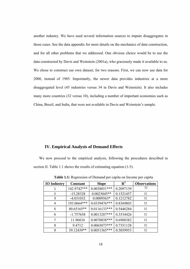
IV. Empirical Analysis of Demand Effects

We now proceed to the empirical analysis, following the procedures described in

section II. Table 1.1 shows the results of estimating equation (1-5).

Table 1.1: Regression of Demand per capita on Income per capita

IO Industry Constant Slope R2 Observations 1 142.9742*** 0.0038051*** 0.2097139 32

2 -15.28328 0.0023045** 0.1521457 32 3 -4.031032 0.0009563* 0.1212782 32 4 193.0664*** 0.0339476*** 0.8369803 32

5 80.65165** 0.0116133*** 0.5446284 32

6 -1.757658 0.0013287*** 0.3534426 32

7 11.96834 0.0070038*** 0.6988382 32

8 9.4712 0.0065073*** 0.7351128 32 9 39.12439** 0.0051365*** 0.5059953 32

19

IO Industry Constant Slope R2 Observations 10 13.72378 0.0031796*** 0.2890346 32 11 14.88692** 0.0015037*** 0.4527326 32 12 6.898497 0.0012931*** 0.3414043 32 13 .718209 0.000307** 0.1318374 32 14 1.374558 0.0001946* 0.0879436 32 15 14.74915 0.0047128*** 0.5061247 32 16 58.66057 0.0200428*** 0.7819555 32 17 -11.68477 0.0093417*** 0.6270361 32 18 22.63568 0.0040878*** 0.5239604 32 19 17.25413 0.0107642*** 0.5853083 32 20 1.346999 0.0062071*** 0.8228002 32 21 52.01612 0.0238611*** 0.5941956 32 22 -42.61408 0.0059848*** 0.2138726 32 23 .9135898 0.002275*** 0.3768318 32 24 3.87524 0.0011259*** 0.5054429 32 25 16.2567 0.0107825*** 0.6851407 32

26+27+28+29 29.82466 0.011787*** 0.7923978 32 30 193.5111 0.0796442*** 0.773784 32 31 8.244092 0.099351*** 0.8430198 32 32 43.54092 0.0335992*** 0.6100405 32 33 23.24115 0.0120991*** 0.6016405 32 34 -6.505804 0.0015168*** 0.2356678 32 35 -.4175622 0.0041357*** 0.4567848 32 36 -5.510763 0.0082493*** 0.3516936 32 37 4.718791 0.013241*** 0.7912711 32 38 -46.10209 0.0276621*** 0.4807185 32 39 -98.49873 0.0955897*** 0.915278 32 40 -1.720086 0.002692*** 0.2685539 32 41 -46.44816 0.0111419*** 0.5531402 32 42 1.198311 0.0019003*** 0.3030404 32 43 -25.87239 0.0135057*** 0.6473367 32 44 102.0238 0.074419*** 0.8486514 32 45 -36.73636 0.0541422*** 0.9125933 32 46 -286.0382* 0.0946093*** 0.8378031 32 47 -120.487 0.0460885*** 0.7546713 32 48 31.06501* 0.0007384 0.0280843 32

Note: For each industry the dependent variable is demand per capita, the independent variable is

income per capita. See equation (1-5). *, **, and *** denote significant at the 10%, 5%, and 1%

precision level, respectively.

20

Not surprisingly, income per capita is a strong determinant in most cases of

consumption per capita. It also noteworthy that seven of the intercepts are significantly

different from zero (and a few others are close to statistic significance), indicating non-

homotheticity.

We can use equation (1-7) to calculate the imputed subsistence consumptions, which

are reported on Table 1.2.15

Table 1.2: Subsistence Consumptions

IO Industry Subsistence Consumption1 153.9228 2 -8.652487 3 -1.279493 4 290.7445 5 114.0668 6 2.065433 7 32.12053 8 28.19477 9 53.90382 10 22.87238 11 19.2135 12 10.61922 13 1.601451 14 1.934494 15 28.3093 16 116.3301 17 15.19437 18 34.39753 19 48.22609 20 19.20674 21 120.6721 22 -25.39377 23 7.4596 24 7.114781 25 47.28151

26+27+28+29 63.73967

15 A word of caution should be useful. Since many of the intercepts are estimated imprecisely, and each subsistence consumption requires all intercepts (see equation 1-7), these are perforce imprecisely estimated as well.

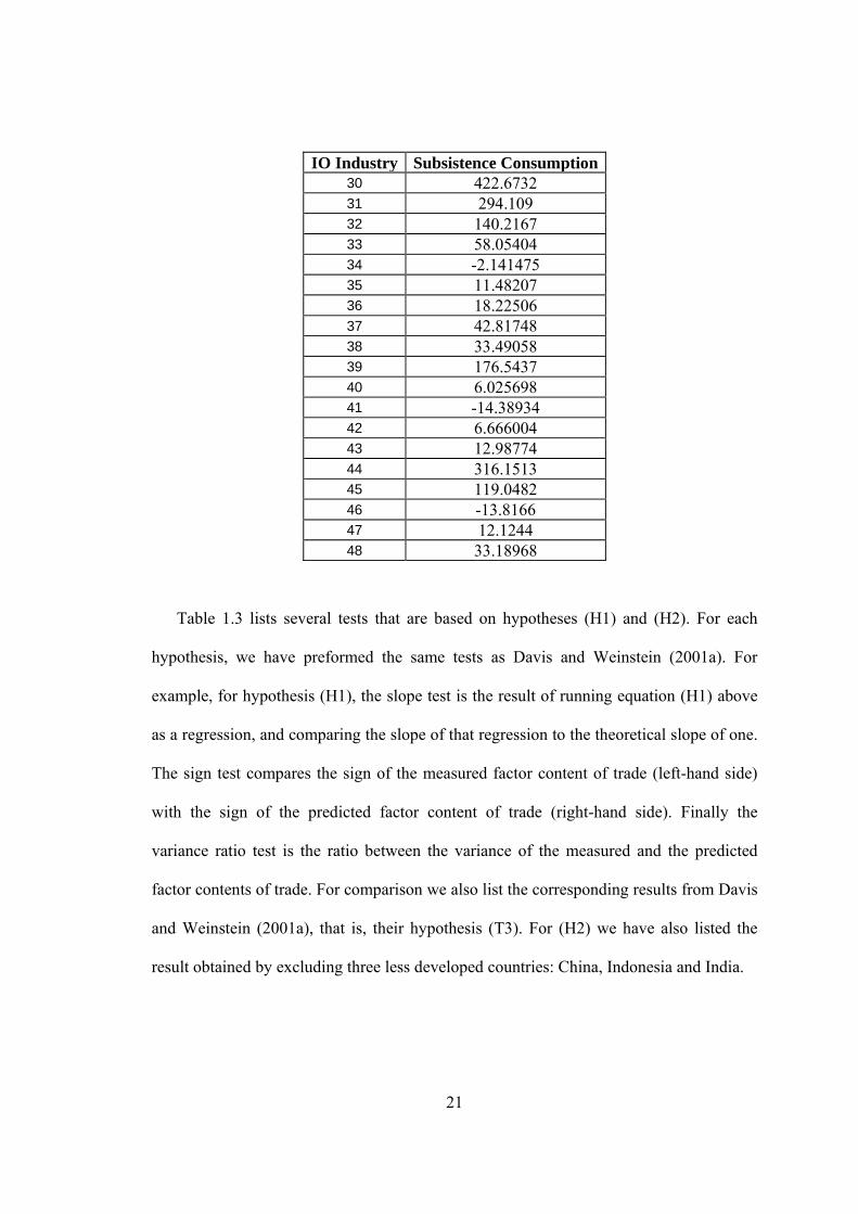
21

IO Industry Subsistence Consumption30 422.6732 31 294.109 32 140.2167 33 58.05404 34 -2.141475 35 11.48207 36 18.22506 37 42.81748 38 33.49058 39 176.5437 40 6.025698 41 -14.38934 42 6.666004 43 12.98774 44 316.1513 45 119.0482 46 -13.8166 47 12.1244 48 33.18968

Table 1.3 lists several tests that are based on hypotheses (H1) and (H2). For each

hypothesis, we have preformed the same tests as Davis and Weinstein (2001a). For

example, for hypothesis (H1), the slope test is the result of running equation (H1) above

as a regression, and comparing the slope of that regression to the theoretical slope of one.

The sign test compares the sign of the measured factor content of trade (left-hand side)

with the sign of the predicted factor content of trade (right-hand side). Finally the

variance ratio test is the ratio between the variance of the measured and the predicted

factor contents of trade. For comparison we also list the corresponding results from Davis

and Weinstein (2001a), that is, their hypothesis (T3). For (H2) we have also listed the

result obtained by excluding three less developed countries: China, Indonesia and India.

22

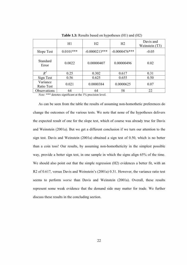
Table 1.3: Results based on hypotheses (H1) and (H2)

H1 H2 H2 Davis and

Weinstein (T3)

Slope Test 0.0101*** -0.0000213*** -0.0000476*** -0.05

Standard Error

0.0022 0.00000407 0.00000496 0.02

R2 0.25 0.302 0.617 0.31 Sign Test 0.56 0.625 0.655 0.50 Variance

Ratio Test 0.021 0.0000384 0.0000625 0.07

Observations 64 64 58 22 Note: *** denotes significant at the 1% precision level.

As can be seen from the table the results of assuming non-homothetic preferences do

change the outcomes of the various tests. We note that none of the hypotheses delivers

the expected result of one for the slope test, which of course was already true for Davis

and Weinstein (2001a). But we get a different conclusion if we turn our attention to the

sign test. Davis and Weinstein (2001a) obtained a sign test of 0.50, which is no better

than a coin toss! Our results, by assuming non-homotheticity in the simplest possible

way, provide a better sign test, in one sample in which the signs align 65% of the time.

We should also point out that the simple regression (H2) evidences a better fit, with an

R2 of 0.617, versus Davis and Weinstein’s (2001a) 0.31. However, the variance ratio test

seems to perform worse than Davis and Weinstein (2001a). Overall, these results

represent some weak evidence that the demand side may matter for trade. We further

discuss these results in the concluding section.

23

V. Conclusions

This chapter has undertaken the research agenda of trying to assess the importance of

the demand side on international trade. We began by asserting that the assumption of

homothetic preferences is not empirically tenable. We derived the predicted factor

content of trade under the assumption that preferences may be non-homothetic, and then

compared it with the measured factor content of trade. We concluded that several tests

yield different messages about the impact of the demand side on trade.

The best support that we could find for the notion that the demand side matters

substantially is that the signs of the predicted factor content and the measured factor

content align themselves better (62% or 66%, instead of 58% of the time) if we calculate

a subsistence consumption pattern for all countries of the world and use it to define non-

homothetic preferences. However, the other tests that we have used hardly perform any

better than if we assume homothetic preferences, which may be excellent news for the

current state of research in trade, in that they would imply that the demand side matters

relatively little and therefore two hundred years of empirical research in international

trade is still allowed to stand! Evidently more research is needed in this important topic.

24

Chapter 2

The Relevance of Trade Costs for the Factor Content of Trade: A Comparison of the Trans-Atlantic and the Intra-European Trade

25

I. Introduction

In this chapter, the hypothesis concerns how the consideration of the existence of

trade costs will help to explain the factor content of trade better than a model that ignores

trade costs. In other words, without trade costs, the factor content of trade cannot fully be

explained. This chapter uses the pair-wise Heckscher-Ohlin-Vanek (HOV) model, a

modified model of the strict HOV model. This chapter selects three types of trade to

explain the bilateral trade by regions. The three types considered are as follows: the trans-

Atlantic trade (between the United States and European countries); the intra-European

trade (among European countries only); and the trans-Atlantic trade that also includes

Australia and Canada. We argue that, compared with the trans-Atlantic trade, the intra-

European trade will have lower trade costs, but the trans-Atlantic trade with Australia and

Canada will have higher trade costs. This chapter draws on research from Davis and

Weinstein (2001a)’s study of 1985 trade data. This chapter makes the argument that trade

costs are an important consideration for the factor content of trade methodology.

II. Literature Review

The original Heckscher-Ohlin (HO) model is a two-country, two-factor, and two-

good model. Vanek (1968) introduces multi-factors and multi-goods into the original HO

model, which became the Heckscher–Ohlin–Vanek (HOV) model. To begin with, we

need to comprehend the HOV model to know what the pair-wise HOV model is. The

26

Heckscher-Ohlin model argues that two countries’ different ratios of their endowment in

factors are the force that creates trade. If two countries have different endowment ratios,

they will trade with each other. Let us assume there are two countries (home and foreign),

two goods (good one and good two), and two factors (capital and labor). We assume that

producers and consumers behave under perfect competition. In addition, the two

countries’ technologies are the same and all firms produce under constant returns to scale.

It is important to note that the factor content of trade methodology originally assumes that

there are no trade costs.

Many trade economists attempted to verify empirically whether the HOV model

works in the real world (Feenstra (2003), p.31). Leamer (1980) argues that Leontief’s

(1953) objects of comparison are not valid. Leontief (1953) compares the factor content

of exports with the factor content of imports, and arrives at the apparent “Leontieff

paradox” that the United States seemed to be a labor-abundant country. By contrast,

Leamer (1980) compares the factor content of consumption with the factor content of net

exports. In his paper, Leamer tests the factor content of trade, defined as FBT, where F

is the vector of net factor (capital and labor) exports, B is the total factor usage matrix,

and T is the net export vector. He uses the same 1947 data from the United States that

Leontief used, trying to replicate Leontief’s findings, but with a different methodology.

With the new methodology, Leamer (1980) finds that the United States is, in fact, a

capital-abundant country.

Markusen’s (1986) important theoretical study investigates how the per capita income

differences between the North, the rich portion of the world, and the South, the poor

portion of the world, can affect trade flows. Both Markusen’s (1986) and Deardorff’s

27

(1998) theoretical articles provide many insights and assume non-homothetic tastes as

well. However, they do not provide additional developments about the factor content of

trade.

Bowen et al. (1987) premises that the methodology that measured factor content of

trade should be the same as the predicted factor content of trade. Their empirical results

could be interpreted as being able to explain the factor content of trade, because they

explain the factor content of trade by more than 50% in their sign test.

Trefler’s (1993) paper, another important study, tries to test the factor content of trade

with strict factor price equalization. However, for the most part, he is not able to fit the

model to the data. While Trefler’s paper concentrates on supply side considerations, he

also extends his theory with demand side considerations, which this dissertation

addressed in chapter 1. Trefler does many tests on the factor content of trade as well as

the bias in consumption. By putting consumption in his model, he diminishes the value of

predicted factor content of trade. Two of Trefler’s other attempts, however, are more

successful in fitting the predicted and the measured factor content of trade. His model

with the Hicks-neutral technological differences has a better result than the standard

HOV model that assumes identical technologies across countries. Furthermore, when he

used a so-called Armington assumption in his model (that is, when he assumed a home-

bias in consumption), he achieves better results than with the standard HOV model that

assumes that preferences are the same everywhere. More specifically, the Armington

assumption is the premise that there is an imperfect substitution between home country

goods and foreign country goods in consumption. The Armington assumption can be

explained with the simple example that people in one country like to consume their

28

country’s products, while people in a different country prefer products from their own

country. Then, one country’s consumption of domestic products will be higher than

predicted in the theory, which helps to explain Trefler’s (1995) “missing trade,” the fact

that predicted factor trade is much larger than observed factor trade. Developing Bowen,

Leamer, and Svikauskas’s (1987) methodology and using industry data, Trefler (1995)

constructs a factor requirement matrix for the United States. He identifies three factors:

capital stock, labor, and land. Again, he uses 33 countries, and his test results using the

standard HOV model are not good. For example, the sign test result is less than 50%.16

To get better results, he studies modified versions of the HOV model and tries to modify

the assumption of strict factor price equalization. A modified form of the factor price

equalization is used when he uses the Hicks-neutral technological differences, and this

modified factor price equalization explains factor trade better than the HOV model with

strict factor price equalization.

Gabaix (1997) also uses a modified factor content of trade model, just as Trefler

(1995) does. Using the same data as Trefler (1995), he tries to find out if one country’s

endowment could be an appropriate predictor in measured factor content of trade. He

uses the strict HOV model and he also uses the methodology of allowing for the Hicks-

neutral technological differences. His results could not explain the factor content of trade

well. However, when he includes demand considerations in his methodology, he observes

slightly better results.

16 As explained in more detail in section IV of this chapter, the sign test is a test that counts the number of observations that have the same sign between the measured factor content of trade and the predicted factor content of trade. It is reported as a percentage of the observations that pass the test.

29

Let us examine in more detail the study by Davis and Weinstein (2001a), who also

use the Heckscher-Ohlin-Vanek model to fit trade data. They use trade data with 10

OECD countries, plus a “Rest of the World” aggregate country. The 10 OECD countries

are Australia, Canada, Denmark, France, Germany, Italy, Japan, the Netherlands, the

United Kingdom, and the United States. The Rest of the World is an aggregate of

Argentina, Austria, Belgium, Finland, India, Indonesia, Ireland, Israel, R.O. Korea,

Mexico, New Zealand, Norway, Philippines, Portugal, Singapore, South Africa, Spain,

Sweden, Thailand, and Turkey. They amend the model in several ways to explain the

factor content of trade. They use two factors: capital and labor. Among the many

amendments to the traditional HOV model, they have introduced non-traded goods and

trade costs using the gravity model of international trade. In their final specification (the

model with most amendments), Davis and Weinstein (2001a) assume a gravity-based

demand determination of demand,17 and thus generate the factor content of consumption

incorporating derived fitted values for import demand and complementary measures of

one country’s own demand. More specifically, they derive the factor content of trade as

follows:

∑ ∑ .

Here, is the technology matrix of country c with the Helpman no-Factor Price

Equalization (FPE) model. Because of no-FPE, each country’s capital to labor ratio (K/L)

will affect all input coefficients in the technology matrix. Note that country c and country

are different. Y T is the net output vector for country c and tradable goods. stands

for the endowment vector for country c. denotes the absorption by country c

17 The gravity model studies bilateral trade flows with size of economy and distance between two countries.

30

produced in country c, and means the predicted absorption by country c produced in

country c. stands for the imports from country c to . denotes the predicted

imports from country c to by fitting from a gravity-model estimation. Davis and

Weinstein generate factor content of consumption incorporating derived fitted values for

import demand and complementary measures of own demand.

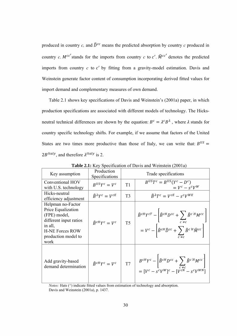
Table 2.1 shows key specifications of Davis and Weinstein’s (2001a) paper, in which

production specifications are associated with different models of technology. The Hicks-

neutral technical differences are shown by the equation: , where stands for

country specific technology shifts. For example, if we assume that factors of the United

States are two times more productive than those of Italy, we can write that:

2 , and therefore is 2.

Table 2.1: Key Specification of Davis and Weinstein (2001a)

Key assumption Production

Specifications Trade specifications

Conventional HOV with U.S. technology T1

Hicks-neutral efficiency adjustment T3

Helpman no-Factor Price Equalization (FPE) model, different input ratios in all, H-NE Forces ROW production model to work

T5

′ ′

′

′ ′

′

Add gravity-based demand determination T7

′ ′

′

Notes: Hats (^) indicate fitted values from estimation of technology and absorption. Davis and Weinstein (2001a), p. 1437.

31

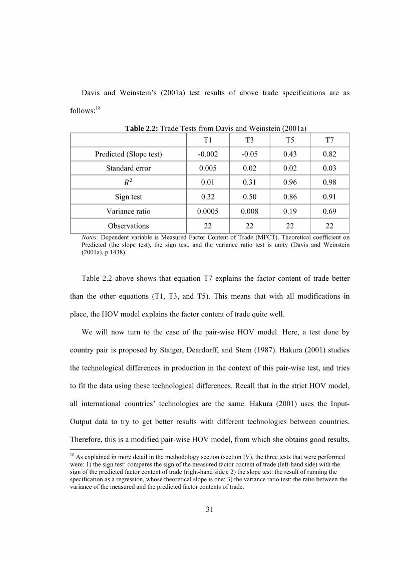
Davis and Weinstein’s (2001a) test results of above trade specifications are as

follows:18

Table 2.2: Trade Tests from Davis and Weinstein (2001a)

T1 T3 T5 T7

Predicted (Slope test) -0.002 -0.05 0.43 0.82

Standard error 0.005 0.02 0.02 0.03

0.01 0.31 0.96 0.98

Sign test 0.32 0.50 0.86 0.91

Variance ratio 0.0005 0.008 0.19 0.69

Observations 22 22 22 22

Notes: Dependent variable is Measured Factor Content of Trade (MFCT). Theoretical coefficient on Predicted (the slope test), the sign test, and the variance ratio test is unity (Davis and Weinstein (2001a), p.1438).

Table 2.2 above shows that equation T7 explains the factor content of trade better

than the other equations (T1, T3, and T5). This means that with all modifications in

place, the HOV model explains the factor content of trade quite well.

We will now turn to the case of the pair-wise HOV model. Here, a test done by

country pair is proposed by Staiger, Deardorff, and Stern (1987). Hakura (2001) studies

the technological differences in production in the context of this pair-wise test, and tries

to fit the data using these technological differences. Recall that in the strict HOV model,

all international countries’ technologies are the same. Hakura (2001) uses the Input-

Output data to try to get better results with different technologies between countries.

Therefore, this is a modified pair-wise HOV model, from which she obtains good results. 18 As explained in more detail in the methodology section (section IV), the three tests that were performed were: 1) the sign test: compares the sign of the measured factor content of trade (left-hand side) with the sign of the predicted factor content of trade (right-hand side); 2) the slope test: the result of running the specification as a regression, whose theoretical slope is one; 3) the variance ratio test: the ratio between the variance of the measured and the predicted factor contents of trade.

32

In particular, Hakura (2001) studies European Community (EC) data19 from the years

1970 and 1980, and shows that it is important to know from where the actual production

came; the history of inputs (intermediate goods) used in making the final goods should be

taken into account. Consider the example of an automobile. Its engine may have come

from country A, the seats from country B, the windows from country C, etc. This vehicle

is assembled in the United States, but its parts came from different countries.

Reimer (2006) also emphasizes the importance of intermediate goods’ trade. He

keeps track of final goods and intermediate goods by country to measure the factor

content of trade in a more efficient way. He concludes that by failing to incorporate

imported intermediate goods correctly, the predicted factor content of trade is overstated.

Both Hakura (2001) and Reimer (2006) argue that the correct measure of the factor

content of trade would take into account the actual factor content of each of these

intermediate goods as they are produced in their own countries.

Staiger et al. (1987) study factor content of trade using data from the United States

and Japan by comparing the measured factor content of trade (left-hand side of the trade

specification) and the predicted factor content of trade (right-hand side of the trade

specification). Relevant to this chapter, they attempt to introduce trade costs. Using

protection in their model caused measured and predicted factor content of trade to be

different. They point out that differences in natural resources and types of workers should

be taken into account when doing research on the factor content of trade. The first

concern is natural resources and their differences across countries. For example, the

amount of arable land in the United States is greater than that in Japan. Staiger et al.

(1987) argue that these differences in natural resources could be a possible reason why 19 She uses four European Community countries: Belgium, France, Germany, and the Netherlands.

33

the sign tests are wrong. The second concern is that there exist many different types of

workers. These workers are comprised of professional workers, technical workers,

managerial workers, administrative workers and so on. Staiger et al. believe that the

United States has more professional and administrative workers who can contribute to the

multinational firms than Japan. The problem with these more diversified types of workers

is that these workers’ incomes are not measured perfectly, which will ultimately reflect

on our ability to measure the factor content of trade. This may be the second reason why

the sign tests of the factor content of trade do not perform well. Staiger et al. argue that if

those two concerns can be solved, the results of sign tests would better explain the factor

content of trade.

Debaere (2003) explains the factor content of trade in the context of the HOV model

using bilateral data. He compares North-South factor content for countries with very

different endowments. He studies the relationship between comparative factor abundance

and bilateral trade between countries. His results explain the factor content of trade,

especially in sign tests. Countries with different endowment ratios (K/L) have different

factor content of trade.

Helpman (1987) predicts that countries with similar size will trade more and proves

this prediction using the OECD countries. Hummels and Levinsohn (1995) revisit

Helpman’s tests using Helpman’s data set comprised of the OECD countries and prove

empirically Helpman’s finding. Hummels and Levinsohn repeat their tests using non-

OECD countries and again empirically prove Helpman’s prediction. According to

Debaere (2005), “intra-industry trade is thought not to matter” with regards to non-OECD

countries (p.250). Debaere (2005) shows that bilateral trade to GDP ratios increases as a

34

results of similarity in GDPs among the OECD country pairs. Debaere also tests

Helpman’s prediction with non-OECD countries and rejects the prediction. Thus, his

result contradicts Hummels and Levinsohn’s findings.

Finally, the paper by Choi and Krishna (2004) argues that when we assume that there

are Ricardian technological differences, theoretical restrictions need to be imposed on the

model. To this purpose, Choi and Krishna (2004) have used Helpman’s (1994)

methodology. Both Helpman (1994) and Choi and Krishna (2004) assume that all

countries have the same technology.

Having described all of the different methodologies, this chapter will use the

methodology that is common to Hakura (2001) and Staiger et al. (1987), along with

Davis and Weinstein’s 1985 data set, in order to perform three tests of the HOV model:

the trans-Atlantic countries’ analysis, the intra-European countries’ analysis, and the

trans-Atlantic countries’ analysis with Australia and Canada. As discussed in the first

chapter of this dissertation, the study of international trade can be divided into a

production side and a consumption side, where the production side has been trade

economists’ main research topic. Therefore, unlike the first chapter, this chapter

concentrates on the production side.

This chapter argues that the trans-Atlantic trade has higher trade costs and therefore,

the factor content of trans-Atlantic trade should not be as well explained as the intra-

European trade. However, many different issues (that are not studied in this chapter) may

complicate that simple prediction. In particular, there is the issue of intra-industry trade,

trade that exists between two countries in the same industry, and that goes both directions

(imports and exports). Such trade is difficult to conform with the Heckscher-Ohlin theory

35

and is more properly the object of the “New Trade Theory” devised by Elhanan

Helpman, Paul Krugman, and others. Note that the European countries have developed

rapidly since 1945, and these economic developments encourage them to trade more,

including intra-industry trade. Their close proximity gives rise to a pattern where these

nations trade mostly amongst themselves, and less with outside trading partners.

First, this chapter tests, the trans-Atlantic analysis using seven countries: the United

States, France, Germany, Italy, the Netherlands, the UK, and Denmark. Second, this

chapter tests the intra-European countries’ trade using six European countries: France,

Germany, Italy, the Netherlands, the UK, and Denmark. Third, this chapter tests the

trans-Atlantic trade with Australia and Canada, the United States, France, Germany, Italy,

the Netherlands, the UK, Denmark, Australia, and Canada.

III. Methodology and Models

This chapter assumes that preferences are identical and homothetic across all

countries; there is perfect competition; for the most part, identical technologies are shared

by all countries; and there are constant returns to scale. It also assumes that factors of

production are perfectly mobile in the long run across sectors, but are perfectly immobile

across countries. Countries have different factor endowments, which cause them to trade.

With the free and costless trade assumption, the price of traded goods will be the same.

We shall assume that there is no measurement error. Davis and Weinstein’s (2001a)

paper deduces a factor trade equation as follows:

36

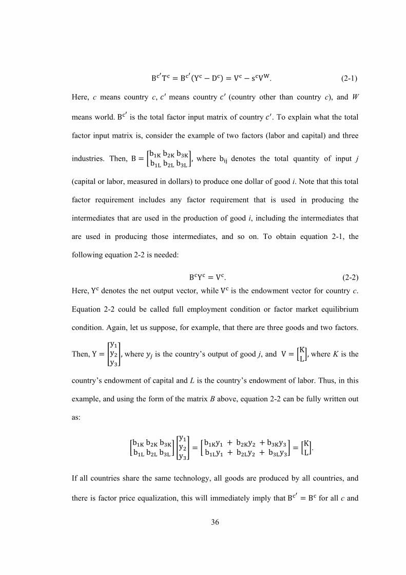
B T B Y D V s VW. (2-1)

Here, c means country c, means country (country other than country c), and W

means world. B is the total factor input matrix of country . To explain what the total

factor input matrix is, consider the example of two factors (labor and capital) and three

industries. Then, Bb K b K b Kb L b L b L

, where b denotes the total quantity of input j

(capital or labor, measured in dollars) to produce one dollar of good i. Note that this total

factor requirement includes any factor requirement that is used in producing the

intermediates that are used in the production of good i, including the intermediates that

are used in producing those intermediates, and so on. To obtain equation 2-1, the

following equation 2-2 is needed:

B Y V . (2-2)

Here, Y denotes the net output vector, while V is the endowment vector for country c.

Equation 2-2 could be called full employment condition or factor market equilibrium

condition. Again, let us suppose, for example, that there are three goods and two factors.

Then, Yyyy

, where is the country’s output of good j, and V KL, where K is the

country’s endowment of capital and L is the country’s endowment of labor. Thus, in this

example, and using the form of the matrix B above, equation 2-2 can be fully written out

as:

b K b K b Kb L b L b L

yyy

b Ky b Ky b Ky b Ly b Ly b Ly

KL

.

If all countries share the same technology, all goods are produced by all countries, and

there is factor price equalization, this will immediately imply that B B for all c and

37

. This is because factor price equalization (along with the other assumptions) implies

that all countries share the same techniques of production. The net exports vector can be

written:

T Y D , (2-3)

where the consumption vector of country c is denoted by D , assuming that consumption

in country c is proportional to YW, which would be the case under homothetic tastes.

Define country c’s consumption share by the notation:

sGDP

GDPW . (2-4)

Then, with the assumption of homothetic tastes, the country’s consumption vector will be

equal to:

D s YW. (2-5)

The original HOV model is F BT V s VW. In other words, the individual

factor content of net trade (exports minus imports) in the original HOV model is denoted

by and . In this example, there

are two factors: capital and labor. Country c is relatively abundant in factor L if

⁄ , and it is abundant in factor K if ⁄ . In this case, both and

have positive signs. Positive signs on both and mean that capital and labor should

both be exported. Conversely, if the signs of and are negative, then those two

factors should be imported. In sum, the formula above gives us , which is country c’s

capital content of net trade and , which is country c’s labor content of net trade. We

will call BT the measured factor content of trade (MFCT) and V s VW the predicted

factor content of trade (PFCT) for the sake of convenience. The various tests of trade

38

(explained in section IV below) consist of checking how close MFCT and PFCT are to

each other. Obviously, if they are the same, the factor content of trade could be fully

explained by the HOV model per Leamer’s (1980) study. Leamer argues that the set of

equation 2-1 “serves as a logically sound foundation for a study of trade-revealed factor

abundance” (p.497).

Hakura (2001) analyzes the pair-wise HOV model like Staiger et al.’s (2001) model.

Hakura studies European Community (EC) data from 1970 and 1980 respectively. With

her methodology, aggregate world data does not need to be estimated for the strict HOV

model. As already mentioned, this chapter will use Hakura’s and Staiger et al.’s

fundamental methodology.

This chapter compares the results of the pair-wise HOV model with different country

groups to show that the existing trade costs fit the factor content of trade better than a

model that ignores trade costs. In other words, without trade costs, factor content of trade

cannot fully be explained.

Let c and m stand for two different countries and introduce the notation:

s GDP

GDPWGDP

GDPW. (2-6)

Why do we use instead of in the pair-wise HOV model? We can think of two

possible reasons. First reason is that the strict HOV model includes world aggregates

when calculating world GDP: . is one component of ,

. In total, this chapter uses nine countries;20 there is some question about

data sums representing world aggregates. In particular, the data for less developed but

very large (hence important in this context) economies is either non-existent or very bad. 20 Refer to Table 2.3.

39

For all of these reasons, calculation of the world aggregates is quite problematic. It is a

major benefit to have a model, the pair-wise HOV model, in which world aggregates are

not included. Second reason is that and will have about the same

size, which should help with ‘heteroskedasticity’ issues. To explain this effect of using

, let us assume that there are two countries, the United States and Japan, and that

those two countries’ expenditure levels are identical. Then, would be equal to one. In

this case, net exports of the United States’ abundant (scarce) factor to the world of

services ought to be greater (less) than Japan’s exports of the same abundant (scarce)

factor. When expenditure levels are different, will not be one. In this case, “

simply controls for the difference in country size and the same interpretations apply”

(Staiger, Deardorff, and Stern (1987), p.453).

Deduction of the pair-wise HOV model is as follows:

To derive the pair-wise HOV model, apply equation 2-1 and 2-6 to two randomly chosen

countries, country c and m:

. (2-7)

With equation 2-3, we deduce:

.

When we apply full employment condition (equation 2-2), we get:

.

By using equation 2-6, we get:

.

40

When we use the assumption that preferences are identical and homothetic, we can write

one country’s consumption as a proportion of the world, and therefore, with equation 2-5

for country m, we get:

.

With canceling out , we get:

.

By equation 2-5, we know that :

.

Here, cancels out and we get:

.

Finally, substituting for the factor content from equation 2-7, we get our testable

equation:

. (2-8)

Note that with the assumption of homothetic preferences, all countries’ consumption

vectors are proportional to each other, which allows us to write s D D .

By calling the left-hand side of the previous equation the measured bilateral factor

content of trade, it can be written as:

B T s B T F s F .

is the measured factor content of net exports from country c; and is the measured

factor content of net exports from country m. Therefore, we can get following equation:

F s F V s V B B D .

41

The left-hand side of equation 2-8 is the Measured Relative Factor Content of Trade

(MRFCT) of the pair-wise HOV model and the right-hand side of the same equation is

the Predicted Relative Factor Content of Trade (PRFCT) of the pair-wise HOV model.

Let us define B B D Q as country c and country m’s technological

differences derived from the general HOV model. If it is assumed that there are only two

factors, capital and labor, then it follows that there are two elements in Q, and .

This chapter conducts empirical tests with the last equation 2-8. If it is assumed that all

countries’ technology is the same (although this does not happen in the real world) with

factor price equalization, then it can be concluded that B and B are the same, and Q is

zero, and we can derive the following equation 2-9:

F s F V s V . (2-9)

By using Davis and Weinstein’s (2001a) data, this chapter will show whether there is

support for the pair-wise HOV model for different groups of countries.

IV. Empirical Tests

This chapter conducts three kinds of tests: the sign test, the slope test, and the

variance ratio test. In Davis and Weinstein (2001a), the sign test compares the sign of the

measured factor content of trade (MFCT) with the sign of the predicted factor content of

trade (PFCT) in the case of equation 2-1: B T B Y D V s VW . In

particular, this test counts the proportion of the same signs between MFCT and PFCT. In

the case of the pair-wise HOV model, the sign test compares the sign of the measured

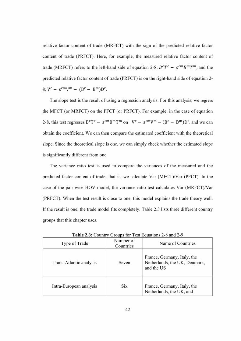
42

relative factor content of trade (MRFCT) with the sign of the predicted relative factor

content of trade (PRFCT). Here, for example, the measured relative factor content of

trade (MRFCT) refers to the left-hand side of equation 2-8: , and the

predicted relative factor content of trade (PRFCT) is on the right-hand side of equation 2-

8: V s V B B D .

The slope test is the result of using a regression analysis. For this analysis, we regress

the MFCT (or MRFCT) on the PFCT (or PRFCT). For example, in the case of equation

2-8, this test regresses B T s B T on V s V B B D , and we can

obtain the coefficient. We can then compare the estimated coefficient with the theoretical

slope. Since the theoretical slope is one, we can simply check whether the estimated slope

is significantly different from one.

The variance ratio test is used to compare the variances of the measured and the

predicted factor content of trade; that is, we calculate Var (MFCT)/Var (PFCT). In the

case of the pair-wise HOV model, the variance ratio test calculates Var (MRFCT)/Var

(PRFCT). When the test result is close to one, this model explains the trade theory well.

If the result is one, the trade model fits completely. Table 2.3 lists three different country

groups that this chapter uses.

Table 2.3: Country Groups for Test Equations 2-8 and 2-9

Type of Trade Number of Countries

Name of Countries

Trans-Atlantic analysis Seven

France, Germany, Italy, the Netherlands, the UK, Denmark, and the US

Intra-European analysis Six France, Germany, Italy, the Netherlands, the UK, and

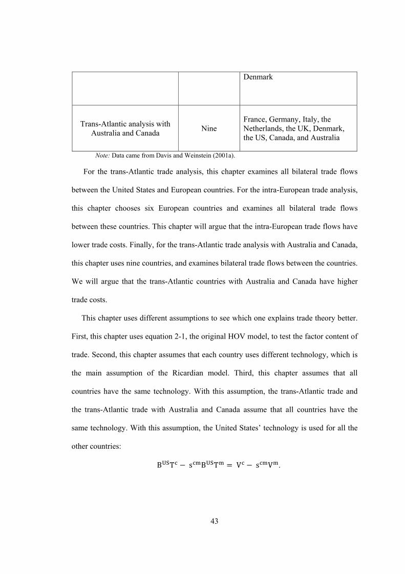
43

Denmark

Trans-Atlantic analysis with Australia and Canada

Nine

France, Germany, Italy, the Netherlands, the UK, Denmark, the US, Canada, and Australia

Note: Data came from Davis and Weinstein (2001a).

For the trans-Atlantic trade analysis, this chapter examines all bilateral trade flows

between the United States and European countries. For the intra-European trade analysis,

this chapter chooses six European countries and examines all bilateral trade flows

between these countries. This chapter will argue that the intra-European trade flows have

lower trade costs. Finally, for the trans-Atlantic trade analysis with Australia and Canada,

this chapter uses nine countries, and examines bilateral trade flows between the countries.

We will argue that the trans-Atlantic countries with Australia and Canada have higher

trade costs.

This chapter uses different assumptions to see which one explains trade theory better.

First, this chapter uses equation 2-1, the original HOV model, to test the factor content of

trade. Second, this chapter assumes that each country uses different technology, which is

the main assumption of the Ricardian model. Third, this chapter assumes that all

countries have the same technology. With this assumption, the trans-Atlantic trade and

the trans-Atlantic trade with Australia and Canada assume that all countries have the

same technology. With this assumption, the United States’ technology is used for all the

other countries:

BUST s BUST V s V .

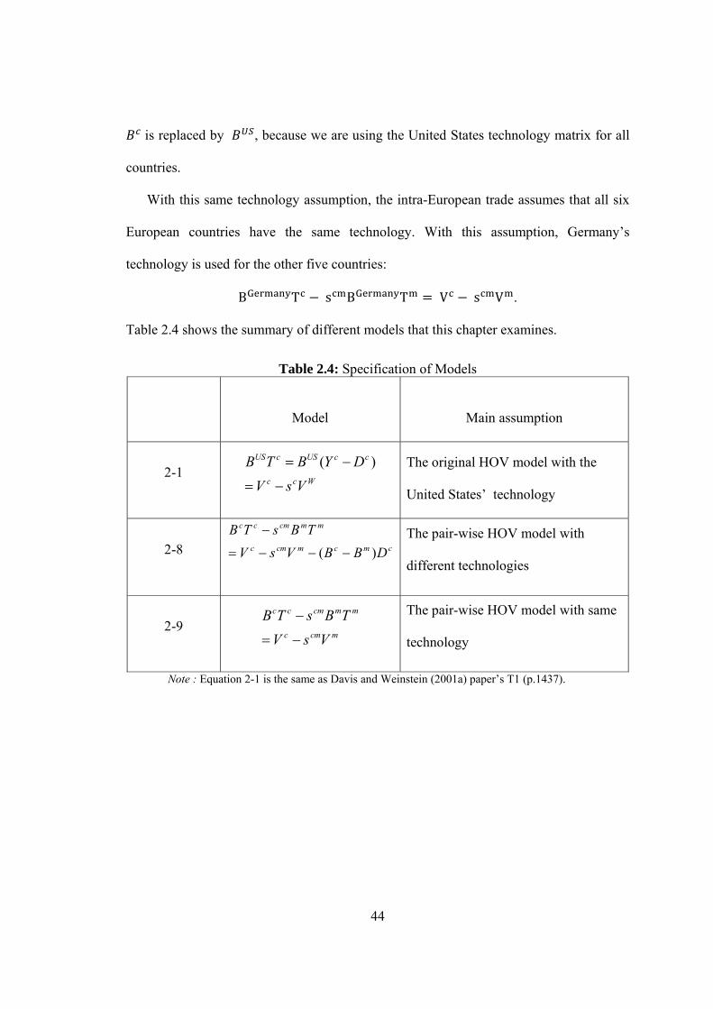
44

is replaced by , because we are using the United States technology matrix for all

countries.

With this same technology assumption, the intra-European trade assumes that all six

European countries have the same technology. With this assumption, Germany’s

technology is used for the other five countries:

BG T s BG T V s V .

Table 2.4 shows the summary of different models that this chapter examines.

Table 2.4: Specification of Models

Model

Main assumption

2-1 Wcc

ccUScUS

VsV

DYBTB

)(

The original HOV model with the

United States’ technology

2-8 cmcmcmc

mmcmcc

DBBVsV

TBsTB

)(

The pair-wise HOV model with

different technologies

2-9 mcmc

mmcmcc

VsV

TBsTB

The pair-wise HOV model with same

technology

Note : Equation 2-1 is the same as Davis and Weinstein (2001a) paper’s T1 (p.1437).

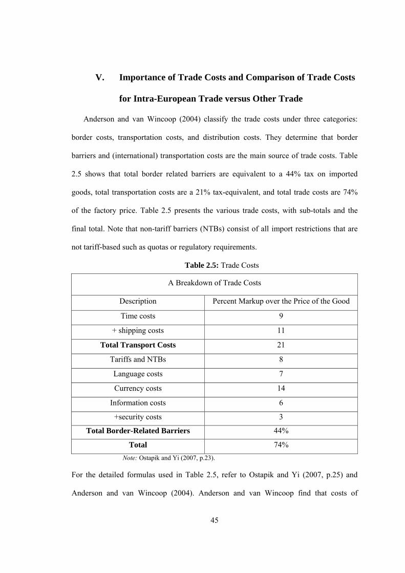
45

V. Importance of Trade Costs and Comparison of Trade Costs

for Intra-European Trade versus Other Trade

Anderson and van Wincoop (2004) classify the trade costs under three categories:

border costs, transportation costs, and distribution costs. They determine that border

barriers and (international) transportation costs are the main source of trade costs. Table

2.5 shows that total border related barriers are equivalent to a 44% tax on imported

goods, total transportation costs are a 21% tax-equivalent, and total trade costs are 74%

of the factory price. Table 2.5 presents the various trade costs, with sub-totals and the

final total. Note that non-tariff barriers (NTBs) consist of all import restrictions that are

not tariff-based such as quotas or regulatory requirements.

Table 2.5: Trade Costs

A Breakdown of Trade Costs

Description Percent Markup over the Price of the Good

Time costs 9

+ shipping costs 11

Total Transport Costs 21

Tariffs and NTBs 8

Language costs 7

Currency costs 14

Information costs 6

+security costs 3

Total Border-Related Barriers 44%

Total 74%

Note: Ostapik and Yi (2007, p.23).

For the detailed formulas used in Table 2.5, refer to Ostapik and Yi (2007, p.25) and

Anderson and van Wincoop (2004). Anderson and van Wincoop find that costs of

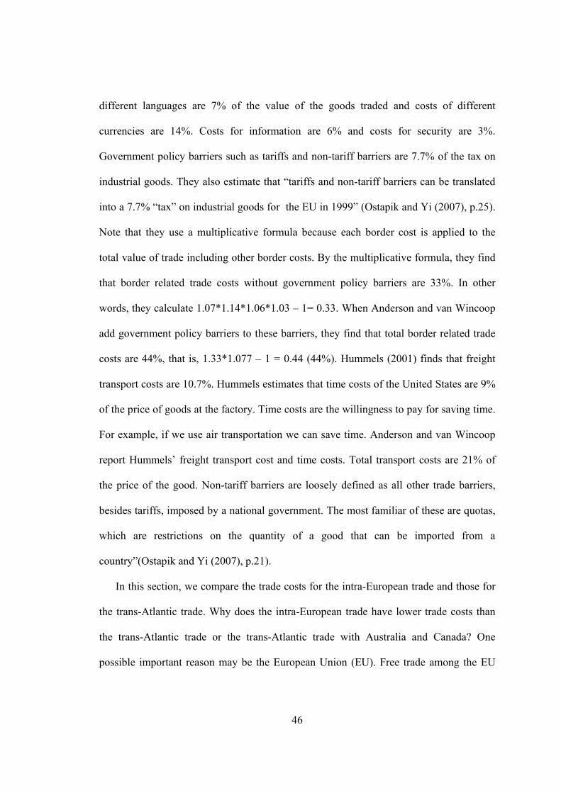
46

different languages are 7% of the value of the goods traded and costs of different

currencies are 14%. Costs for information are 6% and costs for security are 3%.

Government policy barriers such as tariffs and non-tariff barriers are 7.7% of the tax on

industrial goods. They also estimate that “tariffs and non-tariff barriers can be translated

into a 7.7% “tax” on industrial goods for the EU in 1999” (Ostapik and Yi (2007), p.25).

Note that they use a multiplicative formula because each border cost is applied to the

total value of trade including other border costs. By the multiplicative formula, they find

that border related trade costs without government policy barriers are 33%. In other

words, they calculate 1.07*1.14*1.06*1.03 – 1= 0.33. When Anderson and van Wincoop

add government policy barriers to these barriers, they find that total border related trade

costs are 44%, that is, 1.33*1.077 – 1 = 0.44 (44%). Hummels (2001) finds that freight

transport costs are 10.7%. Hummels estimates that time costs of the United States are 9%

of the price of goods at the factory. Time costs are the willingness to pay for saving time.

For example, if we use air transportation we can save time. Anderson and van Wincoop

report Hummels’ freight transport cost and time costs. Total transport costs are 21% of

the price of the good. Non-tariff barriers are loosely defined as all other trade barriers,

besides tariffs, imposed by a national government. The most familiar of these are quotas,

which are restrictions on the quantity of a good that can be imported from a

country”(Ostapik and Yi (2007), p.21).

In this section, we compare the trade costs for the intra-European trade and those for

the trans-Atlantic trade. Why does the intra-European trade have lower trade costs than

the trans-Atlantic trade or the trans-Atlantic trade with Australia and Canada? One

possible important reason may be the European Union (EU). Free trade among the EU

47

members was the original purpose, when the Union was founded 50 years ago. There are

no tariffs in trading between the European Union membership countries.

When we think about transportation perspective, it is safe to assume that the trade

costs of the intra-European trade are less than that of the trans-Atlantic trade.

Transportation costs are one of the examples of trade costs. The intra-European trade has

lower transportation costs than the trans-Atlantic trade because the intra-European trade

has shorter trade distance than its trans-Atlantic counterpart. This finding is related to the

gravity model. The gravity model analyzes bilateral trade flows with economic sizes and

distance between two countries. This result shows that shorter distances mean lower trade

costs.

Table 2.6 below shows each country’s tariff rates, NTBs Ratio,21 and Imports’ Duties.

The European Union has lower tariff rates and NTBs Ratio than the other countries.

Australia has higher tariff rates and Canada has higher NTBs Ratio than the other

countries. Summary statistics show that the European Union has lower Imports Duties

than the other countries.

Table 2.6: Tariff Rates, NTBs Ratio, and Imports Duties

Country Weighted Average

Tariff Rates NTBs Ratio

Imports Duties

1970s 1980s 1990s

United States 3% 0.015 4.37 3.44 2.78

European Union 1% 0.008 0.53 0.06 0.038

Canada 3% 0.151 5.65 3.94 2.44

21 “These NTB ratios are arithmetic and trade weighted NTB coverage ratios, and these ratios are the percentage of tariff lines subject to NTBs” (Anderson and van Wincoop (2004), p.699).

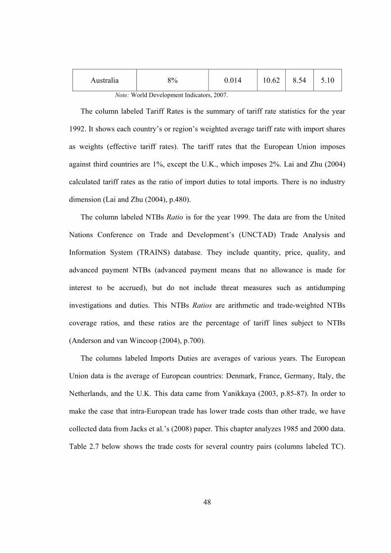
48

Australia 8% 0.014 10.62 8.54 5.10

Note: World Development Indicators, 2007.

The column labeled Tariff Rates is the summary of tariff rate statistics for the year

1992. It shows each country’s or region’s weighted average tariff rate with import shares

as weights (effective tariff rates). The tariff rates that the European Union imposes

against third countries are 1%, except the U.K., which imposes 2%. Lai and Zhu (2004)

calculated tariff rates as the ratio of import duties to total imports. There is no industry

dimension (Lai and Zhu (2004), p.480).

The column labeled NTBs Ratio is for the year 1999. The data are from the United

Nations Conference on Trade and Development’s (UNCTAD) Trade Analysis and

Information System (TRAINS) database. They include quantity, price, quality, and

advanced payment NTBs (advanced payment means that no allowance is made for

interest to be accrued), but do not include threat measures such as antidumping

investigations and duties. This NTBs Ratios are arithmetic and trade-weighted NTBs

coverage ratios, and these ratios are the percentage of tariff lines subject to NTBs

(Anderson and van Wincoop (2004), p.700).

The columns labeled Imports Duties are averages of various years. The European

Union data is the average of European countries: Denmark, France, Germany, Italy, the

Netherlands, and the U.K. This data came from Yanikkaya (2003, p.85-87). In order to

make the case that intra-European trade has lower trade costs than other trade, we have

collected data from Jacks et al.’s (2008) paper. This chapter analyzes 1985 and 2000 data.

Table 2.7 below shows the trade costs for several country pairs (columns labeled TC).

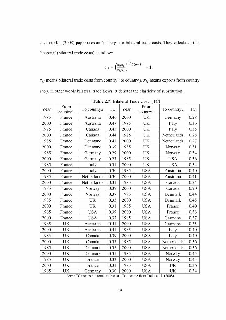
49

Jack et al.’s (2008) paper uses an ‘iceberg’ for bilateral trade costs. They calculated this

‘iceberg’ (bilateral trade costs) as follow:

1.

means bilateral trade costs from country i to country j. means exports from country

i to j, in other words bilateral trade flows. denotes the elasticity of substitution.

Table 2.7: Bilateral Trade Costs (TC)

Year From

country1 To country2 TC Year

From country1

To country2 TC

1985 France Australia 0.46 2000 UK Germany 0.28 2000 France Australia 0.47 1985 UK Italy 0.36 1985 France Canada 0.45 2000 UK Italy 0.35 2000 France Canada 0.44 1985 UK Netherlands 0.28 1985 France Denmark 0.41 2000 UK Netherlands 0.27 2000 France Denmark 0.39 1985 UK Norway 0.31 1985 France Germany 0.29 2000 UK Norway 0.34 2000 France Germany 0.27 1985 UK USA 0.36 1985 France Italy 0.31 2000 UK USA 0.34 2000 France Italy 0.30 1985 USA Australia 0.40 1985 France Netherlands 0.30 2000 USA Australia 0.41 2000 France Netherlands 0.31 1985 USA Canada 0.24 1985 France Norway 0.39 2000 USA Canada 0.20 2000 France Norway 0.37 1985 USA Denmark 0.44 1985 France UK 0.33 2000 USA Denmark 0.45 2000 France UK 0.31 1985 USA France 0.40 1985 France USA 0.39 2000 USA France 0.38 2000 France USA 0.37 1985 USA Germany 0.37 1985 UK Australia 0.41 2000 USA Germany 0.35 2000 UK Australia 0.41 1985 USA Italy 0.40 1985 UK Canada 0.39 2000 USA Italy 0.40 2000 UK Canada 0.37 1985 USA Netherlands 0.36 1985 UK Denmark 0.35 2000 USA Netherlands 0.36 2000 UK Denmark 0.35 1985 USA Norway 0.45 1985 UK France 0.33 2000 USA Norway 0.43 2000 UK France 0.31 1985 USA UK 0.36 1985 UK Germany 0.30 2000 USA UK 0.34

Note: TC means bilateral trade costs. Data came from Jacks et al. (2008).

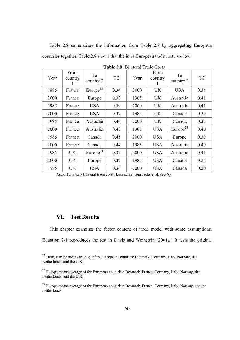
50

Table 2.8 summarizes the information from Table 2.7 by aggregating European

countries together. Table 2.8 shows that the intra-European trade costs are low.

Table 2.8: Bilateral Trade Costs

Year From

country 1

To country 2

TC Year From

country 1

To country 2

TC

1985 France Europe22 0.34 2000 UK USA 0.34

2000 France Europe 0.33 1985 UK Australia 0.41

1985 France USA 0.39 2000 UK Australia 0.41

2000 France USA 0.37 1985 UK Canada 0.39

1985 France Australia 0.46 2000 UK Canada 0.37

2000 France Australia 0.47 1985 USA Europe23 0.40

1985 France Canada 0.45 2000 USA Europe 0.39

2000 France Canada 0.44 1985 USA Australia 0.40

1985 UK Europe24 0.32 2000 USA Australia 0.41

2000 UK Europe 0.32 1985 USA Canada 0.24

1985 UK USA 0.36 2000 USA Canada 0.20 Note: TC means bilateral trade costs. Data came from Jacks et al. (2008).

VI. Test Results

This chapter examines the factor content of trade model with some assumptions.

Equation 2-1 reproduces the test in Davis and Weinstein (2001a). It tests the original

22 Here, Europe means average of the European countries: Denmark, Germany, Italy, Norway, the Netherlands, and the U.K. 23 Europe means average of the European countries: Denmark, France, Germany, Italy, Norway, the Netherlands, and the U.K. 24 Europe means average of the European countries: Denmark, France, Germany, Italy, Norway, and the Netherlands.

51

HOV model using the United States’ technology to construct the matrix of total factor

inputs: . Equation 2-8 tests the pair-wise HOV

model with different technologies: .

Because technologies are different, will not be zero. Equation 2-9 tests

the pair-wise HOV model with the same technology, .

Because technologies are the same, will be zero.

Table 2.9 shows the test results using Davis and Weinstein’s (2001a) data. Rows 3-5

report the slope test (where “predicted” denotes the slope of the measured factor trade on

the predicted factor trade, as explained above); the “standard error” refers to the standard

error of that slope; and R is the results of running that regression. Row 6 reports the sign

test and row 7 reports the variance ratio test. Table 2.9 shows that equation 2-8 using the

trans-Atlantic countries’ data model fits the model best in the case of the slope test.

However, the difference of the slope test result between the trans-Atlantic trade and the

intra-European trade is very small and probably not very significant. Row 6 reports the

sign test’s results. We recall that this test counts the number of same signs between the

measured factor content of trade (or measured relative factor content of trade, the left-

hand side of the testing equations) and the predicted factor content of trade (or predicted

relative factor content of trade, the right-hand side of the testing equation). The sign test

shows, at least when we use Davis and Weinstein’s (2001a) data, that the factor content

of trade using the intra-European countries’ data fits the model better than the factor

content of trade using the trans-Atlantic countries’ data and the trans-Atlantic countries

with Australia and Canada’ data. Note that a sign test close to 50%, as in the case of both

the trans-Atlantic trade and the trans-Atlantic trade with Australia and Canada, is almost

52

no better than a coin toss, and it is close to stating that the model has almost no

explanatory power at all! By contrast, in the intra-European trade, the signs are as

predicted about 80% of the time, which is a major improvement on the predictive power

of the factor content model, when applied to European countries. The result of this sign

test is close to Davis and Weinstein’s of 86% for their model T5 (see Table 2.2), which is

a model that incorporates major amendments of the HOV model, while here it is obtained

without major amendments at all, but simply by restricting trade to the intra-European

trade. Therefore, we see here some evidence suggestive that trade costs are quite

important for the factor content of trade.

We should mention that the variance ratio test, while performing horribly in all cases

(which in the context of Davis and Weinstein’s results is not surprising), does perform

marginally better for the trans-Atlantic trade than for the intra-European trade. However,

given that all such ratios are very small and far from the theoretically-predicted value of

one, we simply state that this may mean that other causes for trade (such as intra-industry

trade, as mentioned in the literature review to this chapter) may be at the root cause for

this. Note that the European economies are arguably more similar to each other than to

the United States and Canada, which would probably cause for a larger proportion of

trade to be intra-industry trade, and therefore less well explained by the Heckscher-Ohlin

model and perhaps better explained by the “New Trade Theory,” which is outside the

scope of this chapter.

Finally, it is worthwhile to compare the from the three different samples. Note that

the regression model restricted to European countries fits much better, at least judging

from the goodness of fit.

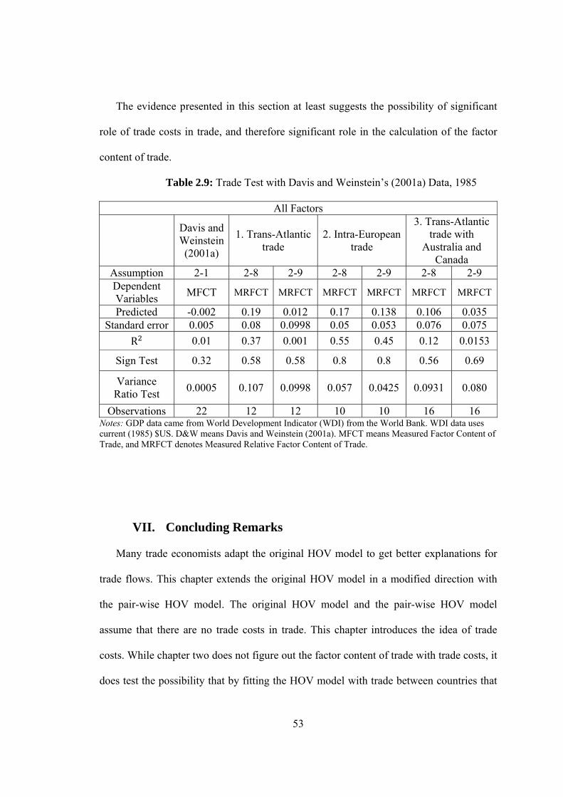
53

The evidence presented in this section at least suggests the possibility of significant

role of trade costs in trade, and therefore significant role in the calculation of the factor

content of trade.

Table 2.9: Trade Test with Davis and Weinstein’s (2001a) Data, 1985

All Factors

Davis and Weinstein (2001a)

1. Trans-Atlantic trade

2. Intra-European trade

3. Trans-Atlantic trade with

Australia and Canada

Assumption 2-1 2-8 2-9 2-8 2-9 2-8 2-9 Dependent Variables

MFCT MRFCT MRFCT MRFCT MRFCT MRFCT MRFCT

Predicted -0.002 0.19 0.012 0.17 0.138 0.106 0.035 Standard error 0.005 0.08 0.0998 0.05 0.053 0.076 0.075

R 0.01 0.37 0.001 0.55 0.45 0.12 0.0153

Sign Test 0.32 0.58 0.58 0.8 0.8 0.56 0.69

Variance Ratio Test

0.0005 0.107 0.0998 0.057 0.0425 0.0931 0.080

Observations 22 12 12 10 10 16 16 Notes: GDP data came from World Development Indicator (WDI) from the World Bank. WDI data uses current (1985) $US. D&W means Davis and Weinstein (2001a). MFCT means Measured Factor Content of Trade, and MRFCT denotes Measured Relative Factor Content of Trade.

VII. Concluding Remarks

Many trade economists adapt the original HOV model to get better explanations for

trade flows. This chapter extends the original HOV model in a modified direction with

the pair-wise HOV model. The original HOV model and the pair-wise HOV model

assume that there are no trade costs in trade. This chapter introduces the idea of trade

costs. While chapter two does not figure out the factor content of trade with trade costs, it

does test the possibility that by fitting the HOV model with trade between countries that

54

have arguably small trade costs, the intra-European countries group, it compares the

results with trade flows between country pairs that have arguably higher trade costs, the

trans-Atlantic countries with Australia and Canada.

This chapter selects three country groups to explain the bilateral trade by regions. The

three regional groups are as follows: the trans-Atlantic countries; the intra-European

countries; and the trans-Atlantic countries with Australia and Canada. The intra-European

countries’ trade will have lower trade costs, however the trans-Atlantic with Australia

and Canada will have higher trade costs.

This chapter compares the importance of the pair-wise HOV models regarding

countries with different technologies and countries with same technology. Equation 2-1

tests the original HOV model with the United States’ technology; Equation 2-8 tests the

pair-wise HOV model with different technology; Equation 2-9 tests the pair-wise HOV

model with the same technology.

By restricting trade to the intra-European trade without major amendments, the sign

test makes substantial progress in this chapter. Therefore, we see here some evidence

suggestive that trade costs are quite important for the factor content of trade.

The pair-wise HOV model explains the intra-European countries’ trade data better

than the trans-Atlantic countries’ trade data with Australia and Canada. This is because

the intra-European trade has smaller trade costs than the trans-Atlantic countries’ trade

with Australia and Canada. This empirical result also shows intuitively that countries

with similar size will trade more like Helpman (1987), Hummels and Levinsohn (1995),

and Debaere (2005) argue, however, this is outside the scope of this chapter.

55

In conclusion, the evidence presented in this chapter is suggestive that trade costs

may play a very significant role in trade, and therefore in the calculation of the factor

content of trade.

56

Chapter 3

Factor Content of Trade with Trade Costs

57

I. Introduction and Brief Overview of Existing Literature

“Trade costs are large, even in the absence of formal barriers to trade and even between

apparently highly integrated economies” (Anderson and van Wincoop (2004), p.1).

The original Heckscher-Ohlin (HO) model assumes two countries, two factors, and

two goods. Paul Samuelson transformed the HO model into a mathematical model, thus

becoming the Heckscher–Ohlin–Samuelson (HOS) model. Vanek (1968) introduces

multi-factors and multi-goods into this model, which becomes the Heckscher–Ohlin–

Vanek (HOV) model. Many trade economists have used the HOV model to verify

empirically whether and how well the HOV model explains the trade data. Davis and

Weinstein (2001a) also use the HOV model to develop their theory.

The original HOV, also known as the strict HOV model, assumes the following: free

trade (no trade costs), perfect competition, identical technologies across countries,

constant returns to scale, different factor endowments across different countries, identical

and homothetic preferences across all consumers in all countries, factors that are

perfectly mobile in the long run across sectors, but perfectly immobile across countries,

and finally no measurement error.

Strictly speaking, the free trade assumption is not realistic in our world. When two

countries trade with each other, trade costs exist. What are these trade costs? With the

assumption that there are consumers and producers, all costs except production costs are

trade costs. Transportation costs, travel costs, and transaction costs are trade costs with

distance effects: greater distance equals greater costs. Transportation costs are needed to

relocate the goods.

58

Currently, many trade agreements, such as the European Union (EU)25 and the North

American Free Trade Agreement (NAFTA),26 make taxes and tariffs much smaller when

accounting for trade costs. This means that transportation costs, travel costs, and

transaction costs are the main components of trade costs. Let us look at the previous

literature regarding the factor content of trade and trade costs.

Samuelson (1952), who studies transportation costs, uses the ‘iceberg’ form to model

transportation costs in his paper in which he studies “transfer problems.” He argues that

firms engaging in international trade try to minimize their trade costs to reap more

benefits. Anderson and van Wincoop’s (2002) paper argues that trade costs are related to

the international trade policy and represent about one-tenth of a country’s gross national

income. Obstfeld and Rogoff (2000) investigate how trade costs are difficult to analyze

and are mixed with many issues in an international economy. Davis’ (1998) paper argues

that developed countries produce more goods and diversified products than

underdeveloped countries, that by contrast, produce simpler products. Also, according to

Davis, developed countries have a more scaled economy than undeveloped countries.

One contribution of Davis’ paper is his demonstration that, depending on the relative size

of trade costs in differentiated and homogeneous industries, market size matters for the

national industrial structure (p.1274). Of course there is an exception to the rule; Davis

25 The EU was established in 1993 and has developed into a single market with 27 membership countries: Austria, Belgium, Bulgaria, Cyprus, Czech Republic, Denmark, Estonia, Finland, France, Germany, Greece, Hungary, Ireland, Italy, Latvia, Lithuania, Luxembourg, Malta, the Netherlands, Poland, Portugal, Romania, Slovakia, Slovenia, Spain, Sweden, and the United Kingdom.

26 The NAFTA was established in 1994 between Canada, Mexico, and the United States.

59

points out the home market effect,27 and therefore market size is not a factor when trade

costs are equal (p.1294).

Edward Ray is one author who has studied the Heckscher-Ohlin model with trade

costs. In particular, Ray’s (1981a) paper deduces trade equations in the presence of

protection. Using data from the United States and some other countries,28 he finds that

tariffs and non-trade barriers are complementary. He also finds that trade protection does

not significantly affect the imports in the United States; this is a result that we should

keep in mind in the context of the results in this chapter (note that Ray’s methodology

was not a factor content methodology). Ray’s (1981b) paper researches imports and trade

barriers. He estimates the equation for trade as a function of trade barriers, and finds that

trade and trade barriers affect each other simultaneously. He derives trade equations,

specifically the import equation, with the Hecksher-Ohlin model. He also derives the

trade barriers equation and considers characteristics of every industry. These industrial

characteristics are the measure of capital intensity and the ratio of skilled labor, indicating

that factor endowments are not only important in the aggregate sense, but also at the

industry level.

Radelet and Sachs (1998) construct a model of trade costs using the CIF/FOB ratio29

as transportation costs. They argue that transportation costs go down as technology

develops. Because government policy affects these transportation costs, they argue that

transportation costs are endogenous variables. They argue that the CIF/FOB ratio

27 The home market effect means that, ceteris paribus, producers prefer to produce within larger countries because producers would face transportation costs on a smaller share of their output (p.1281). 28 The other countries are Canada, the United Kingdom, Germany, Belgium, Italy, France, and Japan. 29 CIF means Cost, Insurance, and Freight and FOB means Free On Board. The CIF price estimates imported items’ cost when they arrive at the importing country. The FOB price estimates imported items’ cost when they are shipped by the exporter.

60

decreases as technology develops and telecommunications become more important.

Radelet and Sachs (1998) argue that countries far apart from each other have more

transportation costs than countries close to each other when they trade. Geographic

isolation and higher shipping costs make it hard to promote exports. When firms sell their

high value-added products, they pay high transportation costs; and they compensate for

these high transportation costs with low wages and low capital incomes. Manufacturing

firms strategize to strengthen their competitiveness in world markets. Radelet and Sachs

(1998) argue that countries with high shipping cost, such as Mongolia, Rwanda, Burundi,

and Bolivia cannot grow according to the export-led growth theory, although these

countries try to reduce tariff rates, and remove quantitative restrictions. This is yet one

more way to see that transportation costs tend to have economically significant impacts.

Davis and Weinstein (2001a) argue that trade costs exist in international trade, but in

very small amounts. When Davis and Weinstein research the volume of trade, they use

distance as a measure of trade costs in the same way that it is used in the gravity model.

They use the following equation to add distance in their import equation:

ln ln d ln ε ).30

denotes predicted imports to country c from country . s means total domestic

absorption. X denotes gross output in country c . d means distance between countries

c and c . means error term. , , and are parameters. When and are zero, there

are no trade costs. Davis and Weinstein (2001a) add the effect of trade costs in their

accounting, and conclude that trade costs can improve the explanatory power of the factor

content of trade. However, it is very important to note, as they write in their paper, that

30 Davis and Weinstein (2001a), p.1429.

61

the use of the gravity model31 is a major theoretical departure from the factor content

methodology, and it is not clear that mixing the two methodologies allows for a clean

model. In this chapter, we do not attempt to mix the two methodologies, rather we

attempt to incorporate the trade costs directly into the factor content methodology.

Deardorff (2004) argues that if there are trade costs, the pattern of trade may not be

well described by the usual measures of comparative advantage. Usual measures of

comparative advantage mean comparing a country’s costs or autarky price to those of the

world (p.3). He explains his theory using comparative advantage methodology and

researches the Ricardian model with trade costs. Deardorff also uses his previous

research (1980) as well as Dixit and Norman’s (1980) book to extend his research and to

construct his model with trade costs. He researches the relationship between

differentiation in the products and trade to uncover a previously unnoticed role of trade

costs. He explains that a country’s net trade depends upon production costs and trade

costs. His conclusion is that factoring in trade costs works in real world trade.

Hummels and Lugovskyy’s (2006) paper nicely explains how to choose and use trade

cost data. They argue that trade costs, specifically transportation costs, are not easy to

collect. Their paper explains that many trade economists use indirect measures for

gathering transportation costs. These indirect measures of transportation costs use

matched partner CIF/FOB ratios. These ratios can be collected from the International

Monetary Fund (IMF) and the United Nations (UN) databases. Hummels and Lugovskyy

also acquire directly measured transportation costs for the United States and the

Netherlands. Hummels and Lugovskyy (2006) compare the following transportation

31 The gravity model studies bilateral trade flows as dependent of the size of economy and distance between two countries.

62

costs: direct measured transportation costs and indirectly measured transportation costs.

They conclude that the IMF CIF/FOB ratios have some errors. These ratios came from

the IMF Direction of Trade Statistics (DOTS). Hummels and Lugovskyy (2006) argue

that the IMF CIF/FOB ratios are quite error-ridden and do not have useful information for

time series or cross-commodity variation, but that these IMF CIF/FOB ratios have some

significant cross-exporter variation (p.1).

Bernard, Jensen and Schott (2006) show that trade costs affect the manufacturing

activities of the United States. They use ad valorem trade costs with a heterogeneous firm

model. If the trade costs decrease, high productivity firms redistribute their economic

activities. Firms with low productivity cannot survive when trade costs decrease. Firms

with high productivity will increase their exports as trade costs are decreased. Bernard et

al.’s contribution was to construct trade costs by industry (p.917). They calculate the

following (p.922):

,

where the left side represents the trade costs for industry i and year t. Thus, trade costs

are the sum of any tariffs32 and freight costs. In the expression above, means ad

valorem duty on industry i and year t; and means freight and insurance costs of

industry i and year t. Bernard, Jensen and Schott (2006) obtained and from

Feenstra’s (1996) paper and database. This database is made up from the United States’

import data. They construct the ad valorem duty (d) and ad valorem freight and insurance

(f) according to the following formula (p.922):

.

32 Here, tariff means ad valorem tariff.

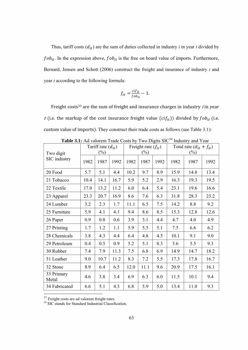
63

Thus, tariff costs ( ) are the sum of duties collected in industry i in year t divided by

. In the expression above, is the free on board value of imports. Furthermore,

Bernard, Jensen and Schott (2006) construct the freight and insurance of industry i and

year t according to the following formula:

1.

Freight costs33 are the sum of freight and insurance charges in industry i in year

t i.e. the markup of the cost insurance freight value divided by i.e.

custom value of imports . They construct their trade costs as follows (see Table 3.1):

Table 3.1: Ad valorem Trade Costs by Two Digits SIC34 Industry and Year

Two digit SIC industry

Tariff rate ( ) (%)

Freight rate ( ) (%)

Total rate ( ) (%)

1982 1987 1992 1982 1987 1992 1982 1987 1992

20 Food 5.7 5.1 4.4 10.2 9.7 8.9 15.9 14.8 13.4

21 Tobacco 10.4 14.1 16.7 5.9 5.2 2.9 16.3 19.3 19.5

22 Textile 17.0 13.2 11.2 6.0 6.4 5.4 23.1 19.6 16.6

23 Apparel 23.3 20.7 16.9 8.6 7.6 6.3 31.8 28.3 23.2

24 Lumber 3.2 2.3 1.7 11.1 6.5 7.5 14.2 8.8 9.2

25 Furniture 5.9 4.1 4.1 9.4 8.6 8.5 15.3 12.8 12.6

26 Paper 0.9 0.8 0.6 3.9 3.1 4.4 4.7 4.0 4.9

27 Printing 1.7 1.2 1.1 5.9 5.5 5.1 7.5 6.6 6.2

28 Chemicals 3.8 4.3 4.4 6.4 4.8 4.5 10.1 9.1 9.0

29 Petroleum 0.4 0.5 0.9 5.2 5.1 8.3 5.6 5.5 9.3

30 Rubber 7.4 7.9 11.3 7.5 6.8 6.9 14.9 14.7 18.2

31 Leather 9.0 10.7 11.2 8.3 7.2 5.5 17.3 17.8 16.7

32 Stone 8.9 6.4 6.5 12.0 11.1 9.6 20.9 17.5 16.1

33 Primary Metal

4.6 3.8 3.4 6.9 6.3 6.0 11.5 10.1 9.4

34 Fabricated 6.6 5.1 4.3 6.8 5.9 5.0 13.4 11.0 9.3

33 Freight costs are ad valorem freight rates. 34 SIC stands for Standard Industrial Classification.

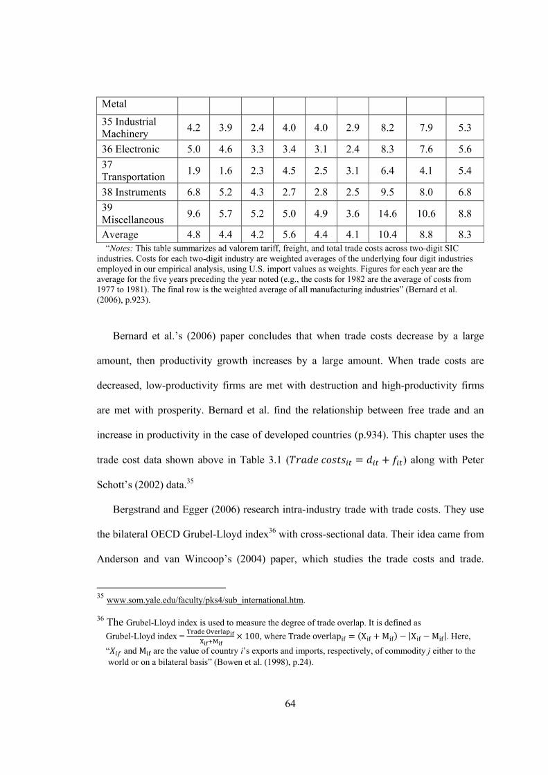
64

Metal

35 Industrial Machinery

4.2 3.9 2.4 4.0 4.0 2.9 8.2 7.9 5.3

36 Electronic 5.0 4.6 3.3 3.4 3.1 2.4 8.3 7.6 5.6

37 Transportation

1.9 1.6 2.3 4.5 2.5 3.1 6.4 4.1 5.4

38 Instruments 6.8 5.2 4.3 2.7 2.8 2.5 9.5 8.0 6.8

39 Miscellaneous

9.6 5.7 5.2 5.0 4.9 3.6 14.6 10.6 8.8

Average 4.8 4.4 4.2 5.6 4.4 4.1 10.4 8.8 8.3 “Notes: This table summarizes ad valorem tariff, freight, and total trade costs across two-digit SIC industries. Costs for each two-digit industry are weighted averages of the underlying four digit industries employed in our empirical analysis, using U.S. import values as weights. Figures for each year are the average for the five years preceding the year noted (e.g., the costs for 1982 are the average of costs from 1977 to 1981). The final row is the weighted average of all manufacturing industries” (Bernard et al. (2006), p.923).

Bernard et al.’s (2006) paper concludes that when trade costs decrease by a large

amount, then productivity growth increases by a large amount. When trade costs are

decreased, low-productivity firms are met with destruction and high-productivity firms

are met with prosperity. Bernard et al. find the relationship between free trade and an

increase in productivity in the case of developed countries (p.934). This chapter uses the

trade cost data shown above in Table 3.1 ( ) along with Peter

Schott’s (2002) data.35

Bergstrand and Egger (2006) research intra-industry trade with trade costs. They use

the bilateral OECD Grubel-Lloyd index36 with cross-sectional data. Their idea came from

Anderson and van Wincoop’s (2004) paper, which studies the trade costs and trade.

35 www.som.yale.edu/faculty/pks4/sub_international.htm. 36 The Grubel-Lloyd index is used to measure the degree of trade overlap. It is defined as

Grubel-Lloyd index = T O

X M100, where Trade overlap X M |X M |. Here,

“ and M are the value of country i’s exports and imports, respectively, of commodity j either to the world or on a bilateral basis” (Bowen et al. (1998), p.24).

65

Bergstrand and Egger (2006) ask the question: Is there a non-linear relationship between

trade costs and the Grubel-Lloyd index? Bergstrand and Egger make the following four

assumptions: first, if trade costs of goods are increased, the volume of intra-industry trade

decreases (here, goods are differentiated goods); second, if the share of intra-industry

trade decreases, trade costs increase; third, if trade costs are increased, the Grubel-Lloyd

index will decrease; fourth, trade costs are nonlinear (p.434-435).

Bergstrand and Egger (2004) assume that there are two countries, two sectors, and

two factors to show trade costs’ role for intra-industry trade, and their paper uses the

following equations in their research on trade costs and intra-industry trade (p.5):

L aLXn x x aLY Y tYY aL n ,

K aKXn x x aKY Y tYY aK n .

Here, means how much labor is needed to produce one unit of good X.

stands for how much capital is needed to produce one unit of good X. means how

much labor is needed to produce one unit of good Y. aKY means how much capital is

needed to produce one unit of good Y. Note that these ‘a’s are the same as the component

of the ‘technology matrix’ in the Davis and Weinstein (2001a) paper and technology

matrix that this dissertation uses; therefore this methodology is closely related to the one

in this chapter. is the demand from the domestic market, while is the demand from

the foreign market. and mean transportation costs for goods X and Y respectively.

Bergstrand and Egger’s (2006) paper uses the following equations (p.436):

L aLXn x x aLY Y tYY aL n ,

K aKXn x x aK n .

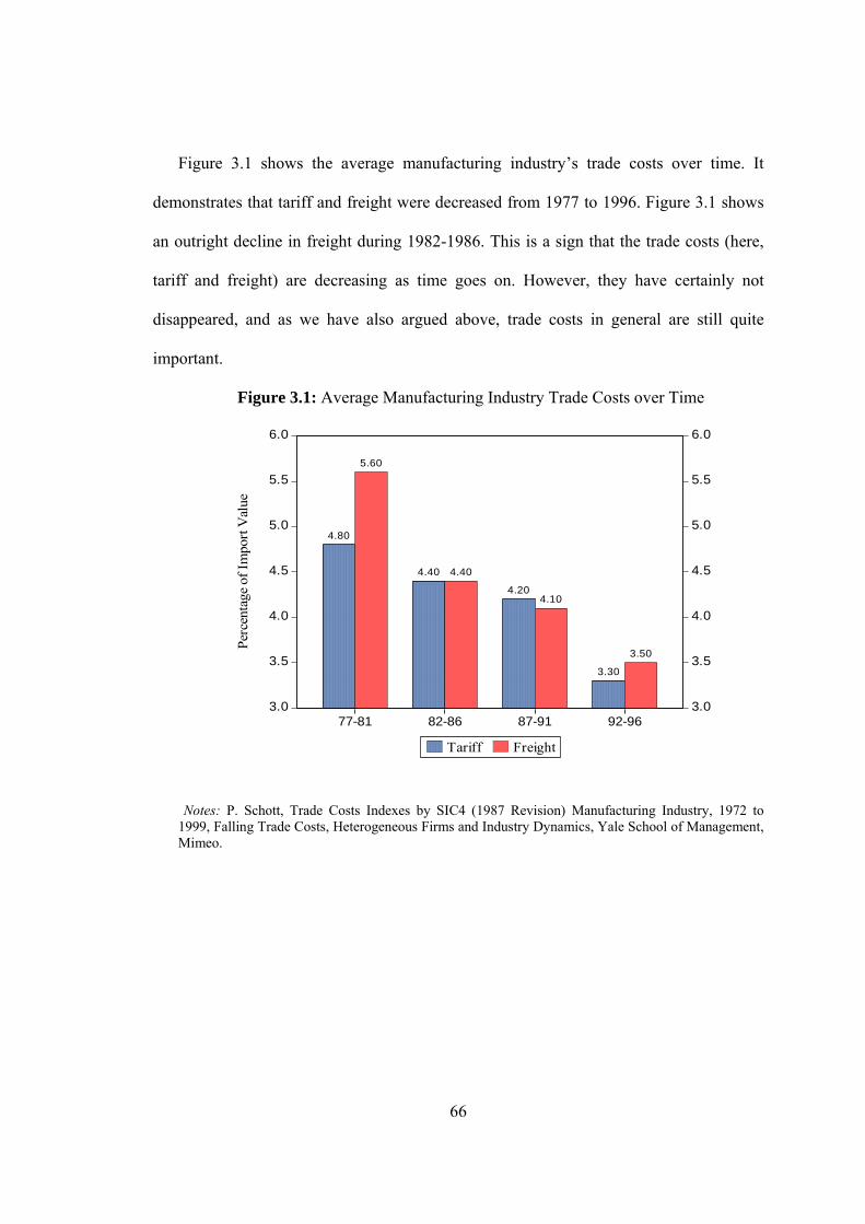
66

Figure 3.1 shows the average manufacturing industry’s trade costs over time. It

demonstrates that tariff and freight were decreased from 1977 to 1996. Figure 3.1 shows

an outright decline in freight during 1982-1986. This is a sign that the trade costs (here,

tariff and freight) are decreasing as time goes on. However, they have certainly not

disappeared, and as we have also argued above, trade costs in general are still quite

important.

Figure 3.1: Average Manufacturing Industry Trade Costs over Time

Notes: P. Schott, Trade Costs Indexes by SIC4 (1987 Revision) Manufacturing Industry, 1972 to 1999, Falling Trade Costs, Heterogeneous Firms and Industry Dynamics, Yale School of Management, Mimeo.

3.0

3.5

4.0

4.5

5.0

5.5

6.0

3.0

3.5

4.0

4.5

5.0

5.5

6.0

77-81 82-86 87-91 92-96

4.80

5.60

4.40 4.40

4.204.10

3.30

3.50

Tariff Freight

Per

cent

age

of I

mpo

rt V

alue

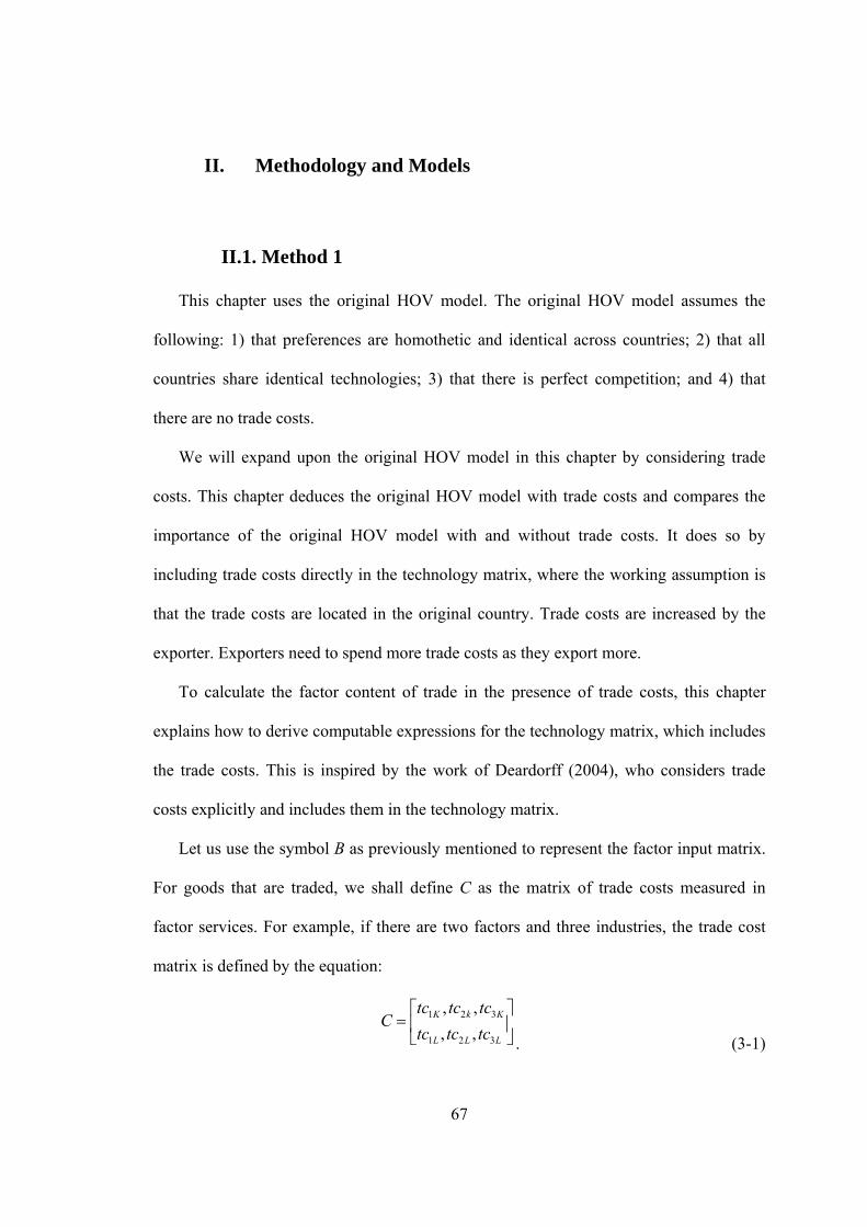
67

II. Methodology and Models

II.1. Method 1

This chapter uses the original HOV model. The original HOV model assumes the

following: 1) that preferences are homothetic and identical across countries; 2) that all

countries share identical technologies; 3) that there is perfect competition; and 4) that

there are no trade costs.

We will expand upon the original HOV model in this chapter by considering trade

costs. This chapter deduces the original HOV model with trade costs and compares the

importance of the original HOV model with and without trade costs. It does so by

including trade costs directly in the technology matrix, where the working assumption is

that the trade costs are located in the original country. Trade costs are increased by the

exporter. Exporters need to spend more trade costs as they export more.

To calculate the factor content of trade in the presence of trade costs, this chapter

explains how to derive computable expressions for the technology matrix, which includes

the trade costs. This is inspired by the work of Deardorff (2004), who considers trade

costs explicitly and includes them in the technology matrix.

Let us use the symbol B as previously mentioned to represent the factor input matrix.

For goods that are traded, we shall define C as the matrix of trade costs measured in

factor services. For example, if there are two factors and three industries, the trade cost

matrix is defined by the equation:

LLL

KkK

tctctc

tctctcC

321

321

,,

,,

. (3-1)

68

Here, ijtc denotes the trade cost in factor j to deliver one unit of good i abroad. Let us

take each country c’s vector of net exports T and divide it into two vectors, one which

contains all rows of T that are positive and zeros (called T ), and one which contains

all rows of T that are negative and zeros (called T ). Note that T T T . In

other words, T and T are the vectors of net exports and net imports, respectively.37

Then, with the assumption that all trade costs are in the exporter country, country c’s

factor content of trade exports is:

F T BT . (3-2)

Furthermore, country c’s factor endowments are used for production and for exports, and

therefore the country’s endowments are given by:

V B D T T , (3-3)

where V is country c’s vector of endowments. The first term on the right is the factor

used in producing goods consumed domestically (where D is consumption and therefore

D T is the total consumption produced domestically), and the second term is total

factor services used in the production and trade of the exported goods. This can also be

written as:

V B D T CT BY CT . (3-4)

Here, is the net output vector for country c.

If we add equation 3-4 for all countries of the world, we have:

VW BYW CTW , (3-5)

37 In this theory, we are ignoring the role of intra-industry trade.

69

where VW, YW, and TW are world endowments of factors, world net output, and world

net exports, respectively (i.e., TW ∑ T ). Comparison between equations 3-2 and 3-

3 shows that:

F V BD . (3-6)

The assumption of identical and homothetic preferences allows us to write one country’s

consumption as a proportion of the world, and therefore D s DW s YW. When we

add D for all countries, we get DW. We define country c’s portion of the consumption by

the notation: s GDP GDPW⁄ .

Subsequently, using equation 3-6 first and then equation 3-5, we can write the factor

content of trade:

F V s BYW V s VW CTW .

Finally, substituting for the factor content of trade from equation 3-2, we get our testable

equation:

T BT V s VW CTW . (3-7)

This amends the basic Davis and Weinstein (2001a) equation by taking into account the

trade cost in factor services (matrix C). 38

All of the variables in equation 3-7 are given by the data of Davis and Weinstein,

except the matrix of trade costs in factor services (C). We have discussed Deardorff

(2004), who also employs a similar matrix. However, in the Ricardian methodology,

Deardorff only considers one factor of production, labor, and therefore he does not have

to model the separation of the cost of trade in labor and the cost of trade in capital. Here,

38 Recall that the basic factor content equation was BT V s VW.

70

we want this separation of the cost of trade in labor services and capital services. The

data appendix of this chapter shows how to calculate the trade costs matrix C.

We will use several different assumptions to do this. This chapter’s basic intention is

to update the factor content of trade model by employing a trade costs matrix. We use

Deardorff’s (2004) basic idea to add the trade costs in the factor content of trade model.

Deardorff (2004) argues that there are two kinds of theories, the law of Ricardian

comparative advantage with no trade costs, and the law of Ricardian local comparative

advantage with trade costs (p.15-17). In the case with no trade costs, he assumes that

there are two countries, country c and c, and two goods, good q1 and q2. The unit factor

input a denotes how many units of labor are needed to produce one unit of q1 in the

country c. a denotes how many units of labor are needed to produce one unit of q2 in

the country c. With no trade costs, country c has a comparative advantage in producing

q139 if the following condition is satisfied:

. (3-8)

In the second case, Deardorff (2004) includes the trade costs, and the result is:

. (3-9)

Country c produces q1 and delivers it to country with additional trade costs, .

means how many units of country c’s labor are needed to deliver one unit of q from

country c to country . Country c does not produce q2 and deliver it to country . Then

there is a country that satisfies equation 3-9. “The countries and could be the 39 Country c strictly does not produce good q2 per Deardorff’s study.

71

same, and either or both could be the same as c or , in which case the associated trade

cost would be zero. Likewise, good q2 could be the same as q1, although this would be

meaningful only if it were delivered to a different country” (Deardorff (2004), p.15-17).

Let us consider why one country makes steel but not wheat. One reason is that when

trade costs are small, there is a comparative advantage in making steel compared to

making wheat. However, when trade costs are large, there are bigger relative costs in

producing steel than wheat, because there are costs in delivering steel. Why does Mexico

export cement to the United States instead of exporting clothes to Europe? The reason is

that Mexico has a comparative advantage in exporting cement to the United States when

compared with exporting clothes to European countries. Mexico has a comparative

advantage in distance, not the costs in producing goods. When we think about the two

cases discussed above −steel and wheat, and cement and cloth− trade costs matter in

trade. When we think that trade costs matter, relatively low trade costs will be a

comparative advantage.

II.2. Method 2

Method 1 is inspired by the work of Deardorff (2004), and method 2 is inspired by

the idea that trade costs are applied to the net exports ( and not directly to the

technology matrix (B). We know that is the vector of net exports and is the

vector of net imports. This method 2 also ignores the role of intra-industry trade. With the

assumption that all trade costs are located in the exporting country, we define country c’s

trade cost vector by the equation:

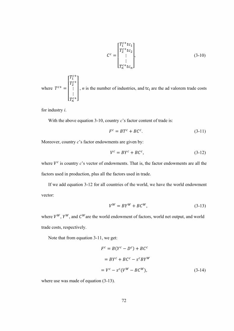
72

, (3-10)

where , n is the number of industries, and tc are the ad valorem trade costs

for industry i.

With the above equation 3-10, country c’s factor content of trade is:

. (3-11)

Moreover, country c’s factor endowments are given by:

, (3-12)

where is country c’s vector of endowments. That is, the factor endowments are all the

factors used in production, plus all the factors used in trade.

If we add equation 3-12 for all countries of the world, we have the world endowment

vector:

, (3-13)

where , , and are the world endowment of factors, world net output, and world

trade costs, respectively.

Note that from equation 3-11, we get:

, (3-14)

where use was made of equation (3-13).

73

Finally, substituting for the factor content of trade from equation 3-11, we get our testable

equation:

. (3-15)

III. Empirical Analysis

We will now proceed to the empirical analysis of the factor content of trade model,

following two procedures in section II. Table 3.2 lists the test results that are based on

method 1 and method 2. We have performed the same tests as Davis and Weinstein

(2001a). The slope test is the result of running the trade specification as a regression,

whose theoretical slope on the predicted factor content of trade is one. The sign test

compares the sign of the measured factor content of trade (left-hand side of the trade

specification) with the sign of the predicted factor content of trade (right-hand side of the

trade specification); and theoretical value of the sign test is one, which means one

hundred percent correct match between the measured and the predicted factor content of

trade. Finally, the variance ratio test is the ratio between the variance of the measured and

the predicted factor contents of trade, and has a theoretical value of one. For comparison,

we also list the corresponding results from Davis and Weinstein’s paper in Table 3.2.

For the original HOV model’s specification with the trade costs in the technology

matrix, method 1, the sign test fits and improves to 65 percent, as shown in Table 3.2.

This is better than relying on a coin toss, and the slope coefficient measured on the

predicted factor content of trade is 0.12, which shows that it is still short of the theoretical

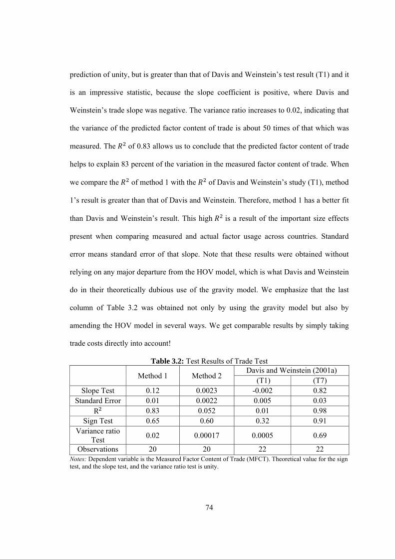
74

prediction of unity, but is greater than that of Davis and Weinstein’s test result (T1) and it

is an impressive statistic, because the slope coefficient is positive, where Davis and

Weinstein’s trade slope was negative. The variance ratio increases to 0.02, indicating that

the variance of the predicted factor content of trade is about 50 times of that which was

measured. The of 0.83 allows us to conclude that the predicted factor content of trade

helps to explain 83 percent of the variation in the measured factor content of trade. When

we compare the of method 1 with the of Davis and Weinstein’s study (T1), method

1’s result is greater than that of Davis and Weinstein. Therefore, method 1 has a better fit

than Davis and Weinstein’s result. This high is a result of the important size effects

present when comparing measured and actual factor usage across countries. Standard

error means standard error of that slope. Note that these results were obtained without

relying on any major departure from the HOV model, which is what Davis and Weinstein

do in their theoretically dubious use of the gravity model. We emphasize that the last

column of Table 3.2 was obtained not only by using the gravity model but also by

amending the HOV model in several ways. We get comparable results by simply taking

trade costs directly into account!

Table 3.2: Test Results of Trade Test

Method 1 Method 2 Davis and Weinstein (2001a)

(T1) (T7) Slope Test 0.12 0.0023 -0.002 0.82

Standard Error 0.01 0.0022 0.005 0.03 R 0.83 0.052 0.01 0.98

Sign Test 0.65 0.60 0.32 0.91 Variance ratio

Test 0.02 0.00017 0.0005 0.69

Observations 20 20 22 22 Notes: Dependent variable is the Measured Factor Content of Trade (MFCT). Theoretical value for the sign test, and the slope test, and the variance ratio test is unity.

75

As we can see from the test results with method 2 in Table 3.2, the fit of the sign test

improves to 60 percent and the slope coefficient increases to 0.0023, relative to Davis and

Weinstein’s results (T1), which shows that it is still short of the theoretical prediction of

unity. The difference of the slope test result between method 2 and Davis and Weinstein

(T1) is very small and not very significant. However, it is an impressive statistic, because

the slope coefficient is positive where Davis and Weinstein’s trade slope was negative.

The variance ratio decreases to the insignificant amount of 0.00017, indicating that the

variance of the predicted factor content of trade still exceeds that of the measured factor

content of trade by a factor of over 5,800. The of 0.052 implies that the regression

equation explains 5.2 percent of the variation in the measured factor content of trade. The

of method 2 is greater than Davis and Weinstein (T1)’s. We conclude therefore that

method 1 seems to be the best method to account for trade costs.

IV. Concluding Remarks

“Trade costs are large on average” (Anderson and van Wincoop (2004), p.86).

Departing from the Davis and Weinstein procedure, we expand upon the original

HOV model by considering trade costs. This chapter deduces the original HOV model

with trade costs, and compares the importance of the original HOV model with and

without trade costs. This first model, method 1, includes the trade costs directly in the

technology matrix, where our assumption is that the trade costs are located in the original

country. To calculate the factor content of trade in the presence of trade costs, this

76

chapter explains how to derive computable expressions for the technology matrix, which

includes the trade costs.

This approach permits us to use the standard evaluations of the original HOV model:

the sign test, the slope test, and the variance ratio test. Using the dataset of 10 countries,

we find evidence supporting the fundamental idea of trade costs inside of the technology

matrix, method 1, with a result of 65 percent for the sign concordance, of 0.12 for the

slope coefficient, and 0.02 for the variance ratio. Our results indicate that the trade costs

inside of the technology matrix are an appropriate modification of the HOV model.

Additionally, this chapter includes trade costs directly in the vector of the net exports,

method 2, and also finds evidence supporting the theory with the same data as method 1.

However, the evidence is weak. With method 2, the sign fit of the sign test improves to

60 percent and the slope coefficient increases to 0.0023; however, the variance ratio test

does not show better results than Davis and Weinstein. Our test results also indicate that

the trade costs in the vector of the net exports are an appropriate modification of the HOV

model, but not as much as the case that the trade costs inside of the technology matrix.

The contribution of this chapter is to show that modifying the HOV model by

including trade costs inside of the technology matrix and trade costs in the vector of the

net exports can establish considerable gains in the predictive performance of the HOV

model.

77

DATA APPENDIX

A. For Chapter One

A contribution of this project was the construction of a new and rich dataset. We hope

that making this new dataset widely available to researchers interested in international

trade and production becomes an important contribution of the chapter. In order to

facilitate the dissemination of the data, we provide in this appendix a full documentation

of the data construction.

The main data sources are the OECD’s Input-Output Tables (henceforth “IO”) and

Structural Analysis database (henceforth “STAN”). See Yamano and Ahmad (2006) and

OECD (2005) for data documentation, respectively. IO provides data on inter-industry

flows for each country for a year around 2000. STAN has data, by country, year and

industry, on production, labor and investment. There are 36 countries in IO, including 28

OECD members (all except Iceland and Mexico), plus 8 nonmember countries

(Argentina, Brazil, China, Chinese Taipei, India, Indonesia, Israel, and South Africa).

Together, these countries accounted for about 90% of world GDP in 2000. In this version

of the chapter we exclude the Russian Federation, Mexico, Estonia and Slovenia, which

represent less than 2% of World GDP.40 Because of data problem, we also exclude four

countries: Luxembourg, Switzerland, Taiwan, and South Africa. The 32 countries are

listed in Table A1. We use the version of the IO files provided by the OECD in February

2009, because the most recent files (November 2007) seem to be somewhat incomplete.

We have STAN data for 27 of those countries. We define two country groups: developed

40 Input-Output tables for Russia are available but they have not been harmonized with the ISIC classification used in IO. IO tables for Mexico, Estonia and Slovenia are not yet available.

78

countries (DC) are those for which GDP per capita is above $15,000, while all other

countries are classified as less developed countries (LDC).41

Table A1: Countries with IO Tables

Country Year STAN

available DC/LDC

Argentina 1997 no LDC

Australia 1998 yes DC

Austria 2000 yes DC

Belgium 2000 yes DC

Brazil 2000 no LDC

Canada 2000 yes DC

China 2000 no LDC

Czech Republic 2000 yes LDC

Denmark 2000 yes DC

Finland 2000 yes DC

France 2000 yes DC

Germany 2000 yes DC

Greece 1999 yes LDC

Hungary 2000 yes LDC

India 1998 no LDC

Indonesia 2000 no LDC

41 We chose this cut-off both because it seemed to lay at a natural break in our sample, and for the very practical reason that we needed to keep a substantial number of LDCs. We used the rgdpl series from the World Penn Tables, which contain real GDP per capita in international dollars (Laspeyres index).

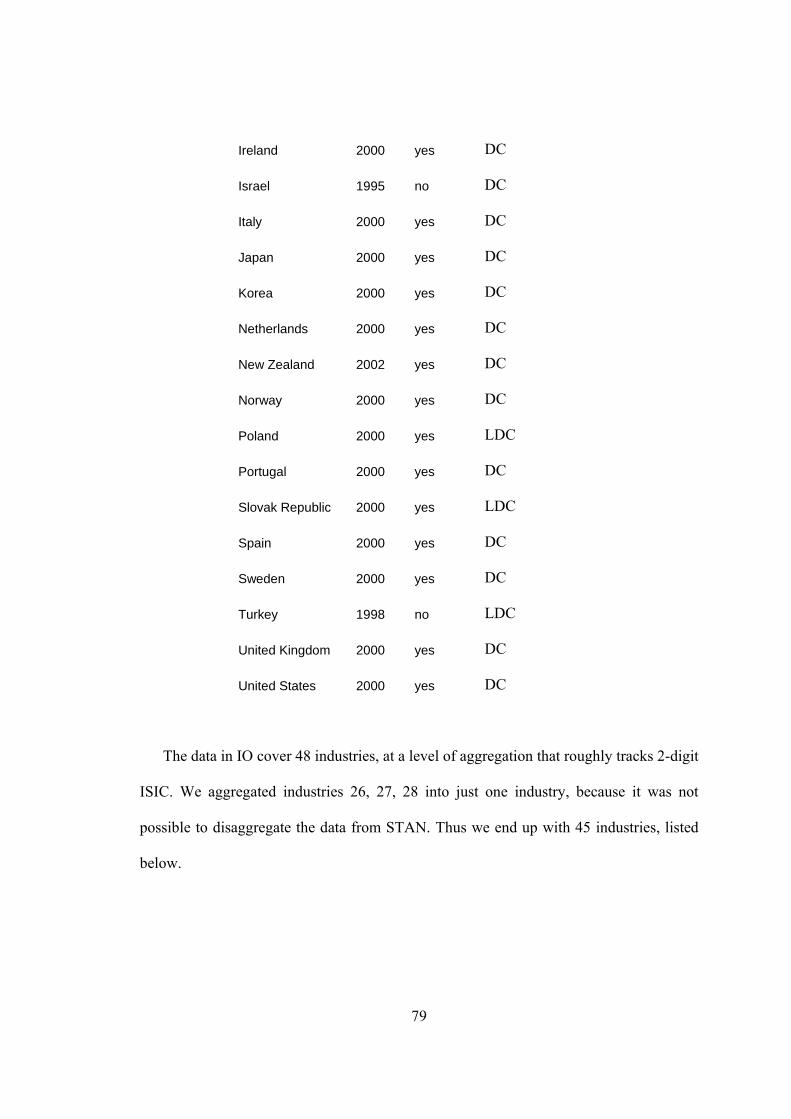
79

Ireland 2000 yes DC

Israel 1995 no DC

Italy 2000 yes DC

Japan 2000 yes DC

Korea 2000 yes DC

Netherlands 2000 yes DC

New Zealand 2002 yes DC

Norway 2000 yes DC

Poland 2000 yes LDC

Portugal 2000 yes DC

Slovak Republic 2000 yes LDC

Spain 2000 yes DC

Sweden 2000 yes DC

Turkey 1998 no LDC

United Kingdom 2000 yes DC

United States 2000 yes DC

The data in IO cover 48 industries, at a level of aggregation that roughly tracks 2-digit

ISIC. We aggregated industries 26, 27, 28 into just one industry, because it was not

possible to disaggregate the data from STAN. Thus we end up with 45 industries, listed

below.

80

Table A2: List of Industries IO Industry Description ISIC Rev.3

1 Agriculture, hunting, forestry and fishing 01+02+05

2 Mining and quarrying (energy) 10-12

3 Mining and quarrying (non-energy) 13-14

4 Food products, beverages and tobacco 15-16

5 Textiles, textile products, leather and footwear 17-19

6 Wood and products of wood and cork 20

7 Pulp, paper, paper products, printing and publishing 21-22

8 Coke, refined petroleum products and nuclear fuel 23

9 Chemicals excluding pharmaceuticals 24, ex. 2423

10 Pharmaceuticals 2423

11 Rubber & plastics products 25

12 Other non-metallic mineral products 26

13 Iron & steel 271+2731

14 Non-ferrous metals 272+2732

15 Fabricated metal products, except machinery & equipment 28

16 Machinery & equipment, n.e.c. 29

17 Office, accounting & computing machinery 30

18 Electrical machinery & apparatus, n.e.c. 31

19 Radio, television & communication equipment 32

20 Medical, precision & optical instruments 33

21 Motor vehicles, trailers & semi-trailers 34

22 Building & repairing of ships & boats 351

23 Aircraft & spacecraft 353

24 Railroad equipment & transport equip. n.e.c. 352+359

25 Manufacturing n.e.c.; recycling (including furniture) 36-37

26+27+28 Electricity, gas, steam and hot water supply 40

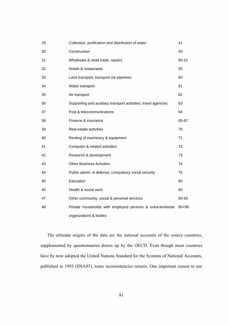
81

29 Collection, purification and distribution of water 41

30 Construction 45

31 Wholesale & retail trade; repairs 50-52

32 Hotels & restaurants 55

33 Land transport; transport via pipelines 60

34 Water transport 61

35 Air transport 62

36 Supporting and auxiliary transport activities; travel agencies 63

37 Post & telecommunications 64

38 Finance & insurance 65-67

39 Real estate activities 70

40 Renting of machinery & equipment 71

41 Computer & related activities 72

42 Research & development 73

43 Other Business Activities 74

44 Public admin. & defense; compulsory social security 75

45 Education 80

46 Health & social work 85

47 Other community, social & personal services 90-93

48 Private households with employed persons & extra-territorial

organizations & bodies

95+99

The ultimate origins of the data are the national accounts of the source countries,

supplemented by questionnaires drawn up by the OECD. Even though most countries

have by now adopted the United Nations Standard for the Systems of National Accounts,

published in 1993 (SNA93), some inconsistencies remain. One important reason to use

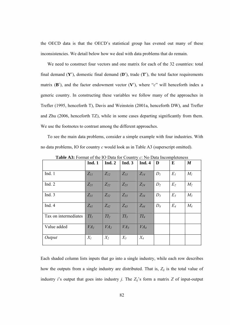
82

the OECD data is that the OECD’s statistical group has evened out many of these

inconsistencies. We detail below how we deal with data problems that do remain.

We need to construct four vectors and one matrix for each of the 32 countries: total

final demand (Yc), domestic final demand (Dc), trade (Tc), the total factor requirements

matrix (Bc), and the factor endowment vector (Vc), where “c” will henceforth index a

generic country. In constructing these variables we follow many of the approaches in

Trefler (1995, henceforth T), Davis and Weinstein (2001a, henceforth DW), and Trefler

and Zhu (2006, henceforth TZ), while in some cases departing significantly from them.

We use the footnotes to contrast among the different approaches.

To see the main data problems, consider a simple example with four industries. With

no data problems, IO for country c would look as in Table A3 (superscript omitted).

Table A3: Format of the IO Data for Country c: No Data Incompleteness Ind. 1 Ind. 2 Ind. 3 Ind. 4 D E M

Ind. 1 Z11 Z12 Z13 Z14 D1 E1 M1

Ind. 2 Z21 Z22 Z23 Z24 D2 E2 M2

Ind. 3 Z31 Z32 Z33 Z34 D3 E3 M3

Ind. 4 Z41 Z42 Z43 Z44 D4 E4 M4

Tax on intermediates TI1 TI2 TI3 TI4

Value added VA1 VA2 VA3 VA4

Output X1 X2 X3 X4

Each shaded column lists inputs that go into a single industry, while each row describes

how the outputs from a single industry are distributed. That is, Zij is the total value of

industry i’s output that goes into industry j. The Zij’s form a matrix Z of input-output

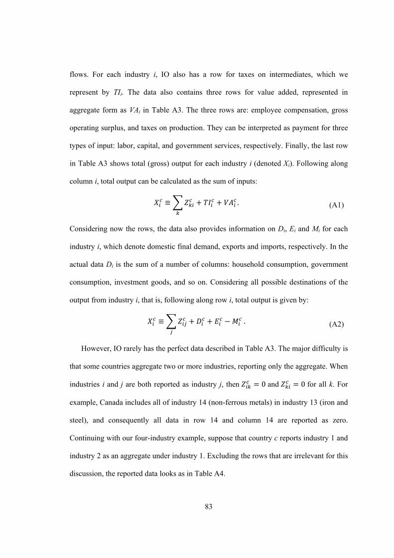
83

flows. For each industry i, IO also has a row for taxes on intermediates, which we

represent by TIi. The data also contains three rows for value added, represented in

aggregate form as VAi in Table A3. The three rows are: employee compensation, gross

operating surplus, and taxes on production. They can be interpreted as payment for three

types of input: labor, capital, and government services, respectively. Finally, the last row

in Table A3 shows total (gross) output for each industry i (denoted Xi). Following along

column i, total output can be calculated as the sum of inputs:

. (A1)

Considering now the rows, the data also provides information on Di, Ei and Mi for each

industry i, which denote domestic final demand, exports and imports, respectively. In the

actual data Di is the sum of a number of columns: household consumption, government

consumption, investment goods, and so on. Considering all possible destinations of the

output from industry i, that is, following along row i, total output is given by:

. (A2)

However, IO rarely has the perfect data described in Table A3. The major difficulty is

that some countries aggregate two or more industries, reporting only the aggregate. When

industries i and j are both reported as industry j, then 0 and 0 for all k. For

example, Canada includes all of industry 14 (non-ferrous metals) in industry 13 (iron and

steel), and consequently all data in row 14 and column 14 are reported as zero.

Continuing with our four-industry example, suppose that country c reports industry 1 and

industry 2 as an aggregate under industry 1. Excluding the rows that are irrelevant for this

discussion, the reported data looks as in Table A4.

84

Table A4: Format of the IO Data for Country c: Some Incomplete Data Ind. 1 Ind. 2 Ind. 3 Ind. 4 D E M

Ind. 1 Z*11+Z*12+

Z*21 +Z*22

0

Z*13+

Z*23

Z*14 +

Z*24

D*1 +

D*2

E*1 +

E*2

M*1 +

M*2

Ind. 2 0 0 0 0 0 0 0

Ind. 3 Z*31 + Z*32 0 Z33 Z34 D3 E3 M3

Ind. 4 Z*41 + Z*42 0 Z43 Z44 D4 E4 M4

Output X*1 + X*2 0 X3 X4

Here, the starred variables represent the latent “true” data. In the event, we do not possess

such data, and it must be imputed. Note that the unstarred variables in Table A4 stand for

all non problematic entries.42 Without risk of confusion, we shall also use unstarred

variables to denote reported aggregate data. Thus, for example, the reported element

(1,1) of matrix Z is .

We are now ready to explain the process of data construction.

42 In reality, such non-problematic industries constitute the large majority of cases.

85

A1. Output:

Output vector Xc for each country is obtained directly from the data (last row of Table

A3). For years other than 2000, all values were deflated to 2000. We used the production

volume index (variable PRODK) to deflate when it is available from STAN. When

PRODK was not available, we used the value added volume index, VALUK. In all cases

in which either volume index was not available at the corresponding industry

aggregation, we used the next available level of aggregation. Thus the data were deflated

according to the equation:

,,

,

,

,,

where is output (in year t) and , is the output deflated for 2000. In the

formula above, , is STAN’s variable PROD (gross output) for country c for

industry I in year t, where industry I is the most disaggregated industry that contains

industry i and for which there is data available. An analogous definition applies for

, .

For countries for which STAN is not available at all (see Table A1), and for Ireland,

which has neither PRODK nor VALUK in STAN, we used the consumer price index to

deflate gross output values. This was done for: Argentina, Brazil, China, India, Indonesia,

Ireland, Israel, Taiwan, and Turkey. All values were converted to U.S. dollars, using the

nominal exchange rate for 2000.43

43 Data for the CPI come from the World Development Indicators (WDI). We used Penn World Tables, version 6.2, for the nominal exchange rate.

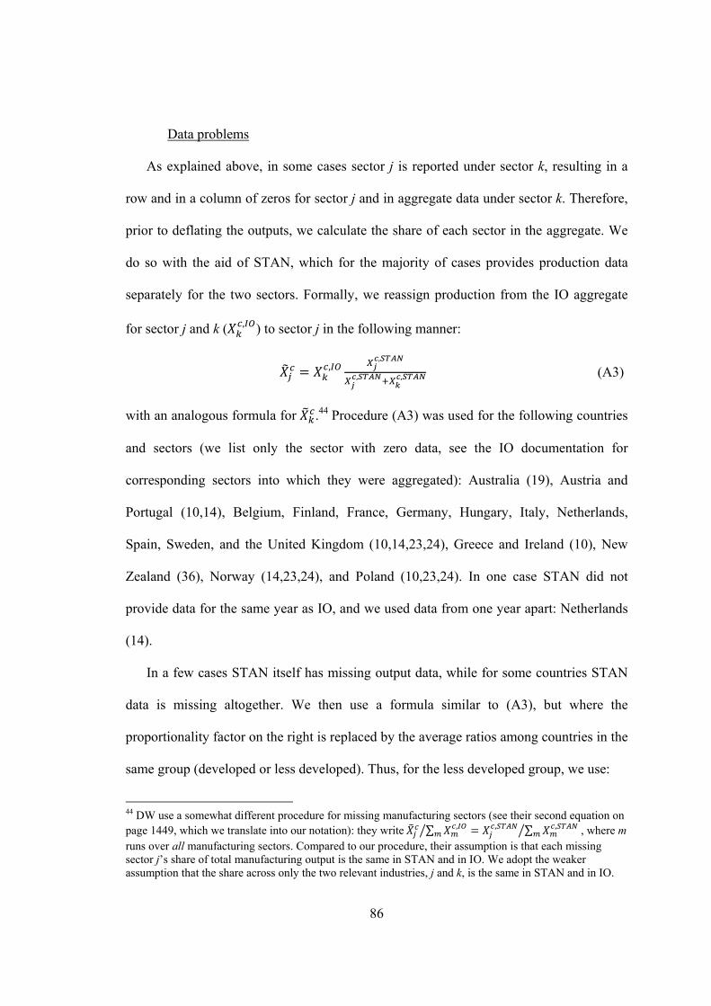
86

Data problems

As explained above, in some cases sector j is reported under sector k, resulting in a

row and in a column of zeros for sector j and in aggregate data under sector k. Therefore,

prior to deflating the outputs, we calculate the share of each sector in the aggregate. We

do so with the aid of STAN, which for the majority of cases provides production data

separately for the two sectors. Formally, we reassign production from the IO aggregate

for sector j and k ( , ) to sector j in the following manner:

,,

, , (A3)

with an analogous formula for .44 Procedure (A3) was used for the following countries

and sectors (we list only the sector with zero data, see the IO documentation for

corresponding sectors into which they were aggregated): Australia (19), Austria and

Portugal (10,14), Belgium, Finland, France, Germany, Hungary, Italy, Netherlands,

Spain, Sweden, and the United Kingdom (10,14,23,24), Greece and Ireland (10), New

Zealand (36), Norway (14,23,24), and Poland (10,23,24). In one case STAN did not

provide data for the same year as IO, and we used data from one year apart: Netherlands

(14).

In a few cases STAN itself has missing output data, while for some countries STAN

data is missing altogether. We then use a formula similar to (A3), but where the

proportionality factor on the right is replaced by the average ratios among countries in the

same group (developed or less developed). Thus, for the less developed group, we use:

44 DW use a somewhat different procedure for missing manufacturing sectors (see their second equation on page 1449, which we translate into our notation): they write ∑ , , ∑ , , where m runs over all manufacturing sectors. Compared to our procedure, their assumption is that each missing sector j’s share of total manufacturing output is the same in STAN and in IO. We adopt the weaker assumption that the share across only the two relevant industries, j and k, is the same in STAN and in IO.

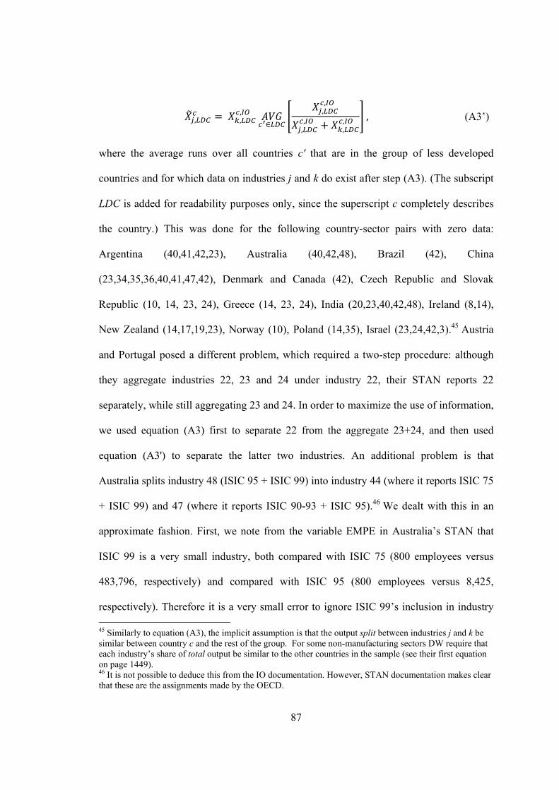
87

, ,, ,

,

,,

,, , (A3’)

where the average runs over all countries c' that are in the group of less developed

countries and for which data on industries j and k do exist after step (A3). (The subscript

LDC is added for readability purposes only, since the superscript c completely describes

the country.) This was done for the following country-sector pairs with zero data:

Argentina (40,41,42,23), Australia (40,42,48), Brazil (42), China

(23,34,35,36,40,41,47,42), Denmark and Canada (42), Czech Republic and Slovak

Republic (10, 14, 23, 24), Greece (14, 23, 24), India (20,23,40,42,48), Ireland (8,14),

New Zealand (14,17,19,23), Norway (10), Poland (14,35), Israel (23,24,42,3).45 Austria

and Portugal posed a different problem, which required a two-step procedure: although

they aggregate industries 22, 23 and 24 under industry 22, their STAN reports 22

separately, while still aggregating 23 and 24. In order to maximize the use of information,

we used equation (A3) first to separate 22 from the aggregate 23+24, and then used

equation (A3') to separate the latter two industries. An additional problem is that

Australia splits industry 48 (ISIC 95 + ISIC 99) into industry 44 (where it reports ISIC 75

+ ISIC 99) and 47 (where it reports ISIC 90-93 + ISIC 95).46 We dealt with this in an

approximate fashion. First, we note from the variable EMPE in Australia’s STAN that

ISIC 99 is a very small industry, both compared with ISIC 75 (800 employees versus

483,796, respectively) and compared with ISIC 95 (800 employees versus 8,425,

respectively). Therefore it is a very small error to ignore ISIC 99’s inclusion in industry 45 Similarly to equation (A3), the implicit assumption is that the output split between industries j and k be similar between country c and the rest of the group. For some non-manufacturing sectors DW require that each industry’s share of total output be similar to the other countries in the sample (see their first equation on page 1449). 46 It is not possible to deduce this from the IO documentation. However, STAN documentation makes clear that these are the assignments made by the OECD.

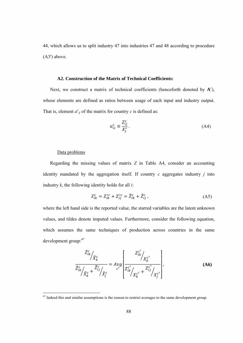
88

44, which allows us to split industry 47 into industries 47 and 48 according to procedure

(A3') above.

A2. Construction of the Matrix of Technical Coefficients:

Next, we construct a matrix of technical coefficients (henceforth denoted by Ac),

whose elements are defined as ratios between usage of each input and industry output.

That is, element acij of the matrix for country c is defined as:

. (A4)

Data problems

Regarding the missing values of matrix Z in Table A4, consider an accounting

identity mandated by the aggregation itself. If country c aggregates industry j into

industry k, the following identity holds for all i:

, (A5)

where the left hand side is the reported value, the starred variables are the latent unknown

values, and tildes denote imputed values. Furthermore, consider the following equation,

which assumes the same techniques of production across countries in the same

development group:47

, (A6)

47 Indeed this and similar assumptions is the reason to restrict averages to the same development group.

89

where the average is performed over all countries c' that do not aggregate industries i and

k, and that are in the same development group (DC or LDC) as country c. Furthermore,

the X’s in the equation above are the values obtained from part A. The solutions to

equations (A5) and (A6) supply the required imputed values for and , which

allows us to disaggregate the columns. This procedure comes with the usual caveats, but

here perhaps in a less dramatic fashion because generally the two industries are similar to

each other. Let us for example suppose that industry k is “Iron and steel,” industry j is

“Non-ferrous metals,” and industry i is “Computers.” Equation (A6) estimates country

c’s proportion of computer usage in iron production, as compared to computer usage in

non-ferrous metals, as similar to the same development group. This is a weaker condition

than assuming that all production techniques are similar across the world.48

Consider now the rows, for which we can write, analogously to equations (A5) and

(A6):

, (A7)

And

, (A8)

where again the average is performed over the countries country c’s development group.

The first equation provides an accounting identity that must necessarily hold.49 Equation

48 That would be assuming ⁄ , which is what DW do (see also footnote 26). Note that an alternative to the methodology in equations (A5) and (A6) is to separate the columns in the same proportions as outputs. However, that would not use any information about techniques of production from other countries. Suppose for example that computers are 2% of the input in iron on average, but are 4% of the input in non-ferrous metals. If we split the columns according to the proportion of the outputs, we will obtain two identical technical coefficients, ignoring the expectation that one should be double of the other. 49 The reader familiar with input-output methodology will recognize a resemblance between our methodology and the well-known RAS method for updating input-output matrices with limited information (see Miller and Blair 1985).

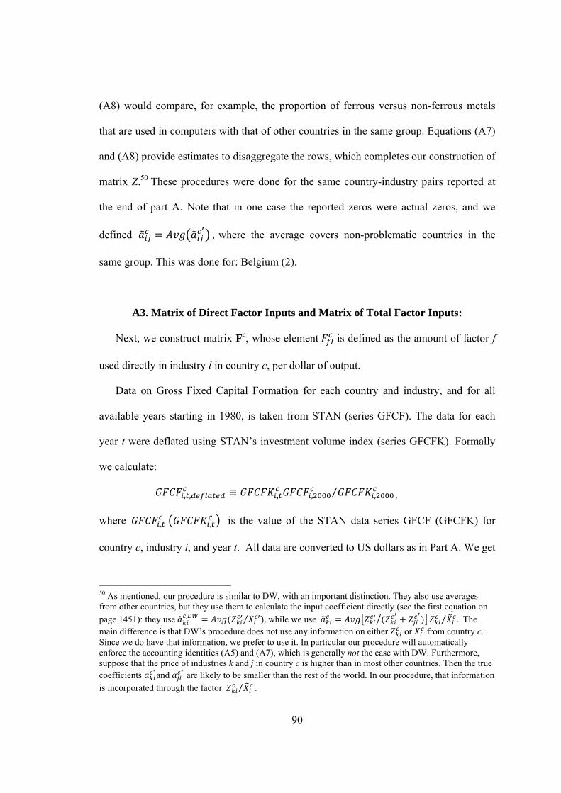
90

(A8) would compare, for example, the proportion of ferrous versus non-ferrous metals

that are used in computers with that of other countries in the same group. Equations (A7)

and (A8) provide estimates to disaggregate the rows, which completes our construction of

matrix Z.50 These procedures were done for the same country-industry pairs reported at

the end of part A. Note that in one case the reported zeros were actual zeros, and we

defined , where the average covers non-problematic countries in the

same group. This was done for: Belgium (2).

A3. Matrix of Direct Factor Inputs and Matrix of Total Factor Inputs:

Next, we construct matrix Fc, whose element is defined as the amount of factor f

used directly in industry l in country c, per dollar of output.

Data on Gross Fixed Capital Formation for each country and industry, and for all

available years starting in 1980, is taken from STAN (series GFCF). The data for each

year t were deflated using STAN’s investment volume index (series GFCFK). Formally

we calculate:

, , , , , ,⁄

where , , is the value of the STAN data series GFCF (GFCFK) for

country c, industry i, and year t. All data are converted to US dollars as in Part A. We get

50 As mentioned, our procedure is similar to DW, with an important distinction. They also use averages from other countries, but they use them to calculate the input coefficient directly (see the first equation on

page 1451): they use , ,⁄ while we use .⁄ The main difference is that DW’s procedure does not use any information on either or from country c. Since we do have that information, we prefer to use it. In particular our procedure will automatically enforce the accounting identities (A5) and (A7), which is generally not the case with DW. Furthermore, suppose that the price of industries k and j in country c is higher than in most other countries. Then the true coefficients and are likely to be smaller than the rest of the world. In our procedure, that information is incorporated through the factor ⁄ .

91

an estimate of the initial capital by multiplying data series KAPW (capital per worker)

from PWT by series LF (labor force) from WDI for the initial year. This yields aggregate

capital for country c and year t0. We deflate it according to the formula:

, , , , ,⁄ ,

where , , is the value of the STAN data series GFCF (GFCFK)

for country c, and year t for the aggregate economy. Finally , is distributed

across the different industries according to the proportion of the Gross Surplus data from

IO, yielding , , .

We then use the perpetual inventory method to construct a stock of capital for each

country and industry in the year of interest. Thus the capital stock in country c and

industry i at the beginning of year 2000 is defined as:

, , 1 1 , , , (A9)

where t0 =1980, the depreciation rate is δ=0.133, and is the initial capital stock in

country c and industry i. To estimate we first obtain aggregate capital stock from the

Penn World Tables, version 5.6 (the last for which there is capital stock available) which

is in 2000 US dollars. 51 Then we distribute it among the different industries according to

each industry’s Gross Operating Surplus (which for country c and industry i we denote by

), available from IO. Note that in some cases (precisely the same as listed at the end of

part A) we first need to impute values for when aggregation wrongly implies that they

would be zero. Formally, if sectors j and k are both reported under sector k, we calculate:

51 We calculated it with the approximation KAPW*POP, where KAPW is Nonresidential Capital Stock per Worker and POP is population.

92

, (A10)

with an analogous formula for sector k. This all that is needed for the calculation of the

capital stock (equation A9).

Labor compensation data by country and industry are also taken from STAN

(variable LABR).52

We then divide both the factor data by the corresponding output to obtain the

elements of matrix Fc. Finally, for each country we construct the matrix of total (direct

plus indirect) factor input requirements as:

. (A11)

The interpretation of equation (A11) is straightforward. Post-multiplying it by (I-Ac) and

rearranging, we obtain: ∑ , where is element (fi) of matrix Bc. It is

given by the direct factor input ( ) plus the sum for each industry j of the indirect factor

input ( ), where the latter in turn takes into account all intermediate inputs to

industry i.

Data problems

In some instances investment data in STAN are at a more aggregated level than the

45 IO industries. In those instances we use equation (A9) to calculate the capital stocks at

the most disaggregated levels available, and then distribute the capital stocks for each

52 DW use the actual number of employees. If wages were equalized within each country (though not necessarily across countries), then the two are approximately equivalent (although ours would take into account part-time and over-time labor). However, with differences in wages across industries, using the currency as the unit of labor is equivalent to using “efficiency units,” with some advantage.

93

industry according to the proportions of each industry’s Gross Operating Surplus

(variable in IO).

For Japan, and for the eight countries without STAN, there was no investment data

available from STAN, so we used a different approach. We obtained the aggregate gross

fixed capital formation series (GFCF) from the World Bank’s World Development

Indicators, in constant 2000 US dollars. After using the perpetual inventory method to

construct the aggregate capital stock at the beginning of 2000 (where the initial capital

stock is still given by the Penn World Tables), we distributed it among the different IO

industries according to the proportions of each industry’s Gross Operating Surplus. Since

Gross Operating Surplus is not available for Argentina and India and we use Value

Added instead.

In some cases the variable in IO turns out to be negative, rendering it useless for

the proportions described in the previous two paragraphs. We then use output as the

proportions to distribute the capital stocks across industries.

For some country-industry pairs we could also not obtain investment information

from STAN at any but the most aggregate level. In those cases we used the same

methodology as for Japan, but restricted to the problematic industries. This was done for:

France (2, 3, 6), New Zealand (6, 7, 16-24), Norway (8, 9) and Portugal (2, 3).

For six countries there was no aggregate capital stock from the Penn World Tables,

which affects our calculation of . We estimated using the proportion between

initial capital and capital accumulation from the remaining countries in the LDC group

(of which all the problematic countries were part). Specifically we calculated:

94

11

∑ 1 , ,

1

, , ,

where the average runs over all LDC countries with initial capital data from the Penn

World tables, and t is country c’s initial year in equation (A9). This was done for: Czech

Republic, Hungary, Slovak republic, Brazil, China, and Indonesia.

For labor compensation, in some cases the data in STAN were also more aggregated

than the 45 IO industries. In those instances we distributed aggregate employment across

the different industries according to the proportions of the Compensation of Employees

variable for country c and industry i (which we denote by ), available in IO. In the case

of Argentina and India, Compensation of Employees is also not available, and we use

Value Added instead.

A4. Final Demand, Trade, and Endowments:

The vector of total final demand is constructed as:

. (A12)

Using equation (A4) it can be easily seen that this is equivalent to: Yc = (I – Ac)Xc. The

vector of factor endowments for country c, denoted by Vc, is constructed as:

.

This is tantamount to assuming full employment of factors. Note that

, as it should.

95

The net trade vector is given by:

,

where we recall that Ec and Mc are the export and import vectors for country c,

respectively. Tc is deflated to 2000 with the same deflators used for output, that is:

, , , ,⁄ ,

where ,

and ,

are the elements of the trade and output vectors given in year t.

Finally, Tc is converted to dollars in the same way as before.

The vector of final domestic demand Dc is constructed by adding the columns in the

IO tables for household final consumption (HHFC), final consumption by non-profit

institutions serving households (NPISH), final consumption expenditures by government

(GGFC), gross fixed capital formation (GFCF), changes in inventories, and valuables.

For ease of presentation those columns were combined into one in Tables A3 and A4.

Data problems

Again we need to address the cases where IO collapses sector j into sector k, and

therefore we have zero exports and zero imports reported for industry j. Fortunately, for

the majority of cases STAN provides export and import information by industry and we

disaggregate exports and imports in a way similar to equation (A3). For example, for

exports in industry j, we calculate:

,,

, , ,

where , denotes exports in industry j in country c, available from STAN.

Analogous procedures were used for exports in industry k and for imports in both

96

industries. This was done for: Australia (17, 19), Austria, Ireland, Portugal (9, 10, 13, 14,

22, 24), Belgium, Czech Republic, Finland, France, Germany, Greece, Hungary, Italy,

Netherlands, Norway, Slovak Republic, Spain, Sweden and United Kingdom (9, 10, 13,

14, 22, 23, 24), New Zealand (13, 14, 17, 18, 19, 23, 24), Poland (2, 3, 9, 10, 13, 14, 22,

23, 24).

In some cases where STAN does not have trade data but has production data. For the

case where industry j is collapsed into industry k, we use the following expression

directly for the trade vector element j:

, ,,

, , , (A13)

with an analogous expression for sector k. This is tantamount to assuming that the

country’s share of exports in industry j (compared to the total exports in industries j and

k) is given by the share in production. For example, if we only know the aggregate

exports in pharmaceuticals and in chemicals, but we know that the chemical industry is

nine times larger than the pharmaceutical industry, we attribute 10% of the exports to

pharmaceuticals, and the remainder to chemicals. 53 This procedure was done for:

Australia (48), Canada (42, 43), Denmark (23, 24), New Zealand (35, 36), Poland (34,

35).

Note that we adjusted Xc, Ec, and Mc, for the most part, based on each country’s

STAN proportions, while matrix Zc was adjusted based partly on averages of other

53 As before, we point out the limitations of this procedure. The imputation in equation (A13) will be less exact to the extent, for example, that country c has comparative advantage in chemicals and comparative disadvantage in pharmaceuticals. The working assumption is that the two industries in question are similar enough for comparative advantage to be similar. This is the best (weakest) assumption that we can adopt, given the data limitations.

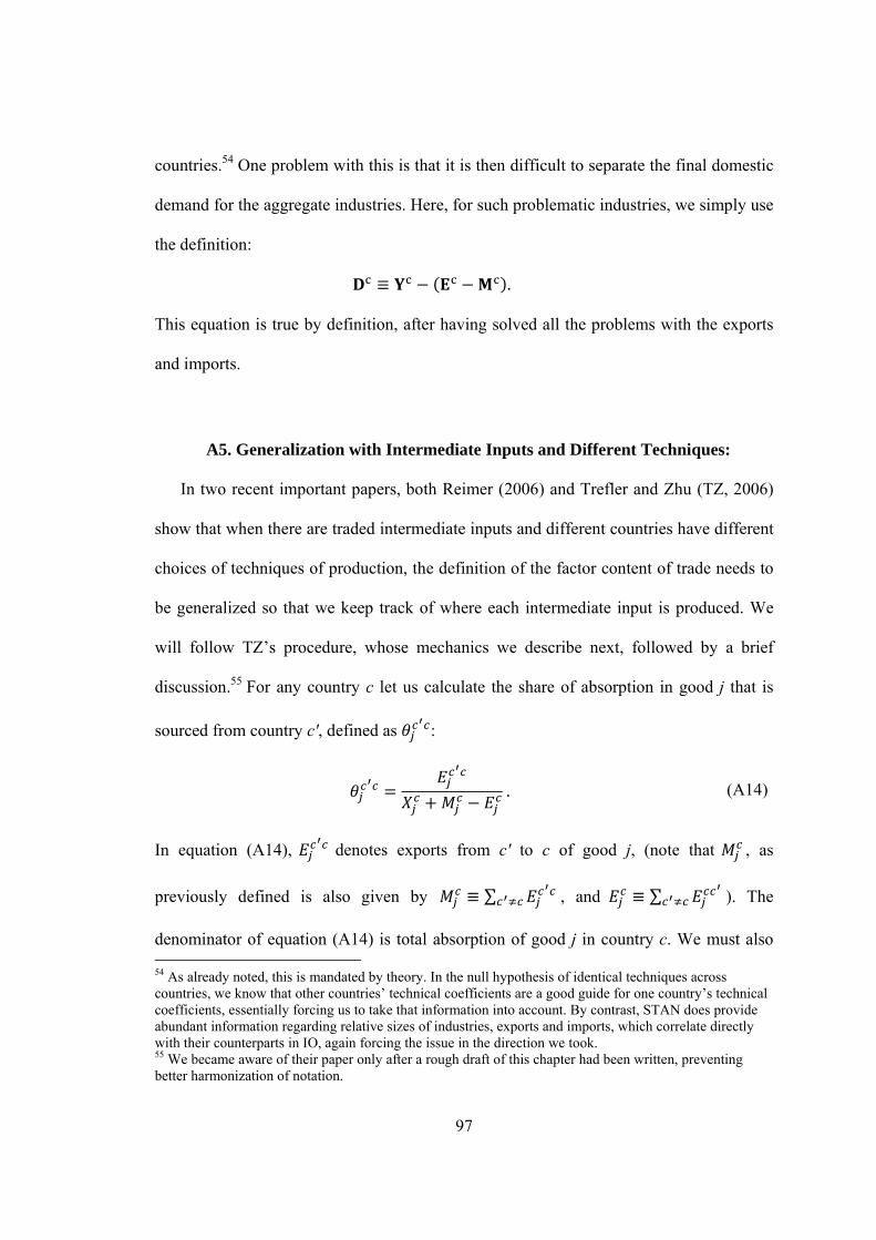
97

countries.54 One problem with this is that it is then difficult to separate the final domestic

demand for the aggregate industries. Here, for such problematic industries, we simply use

the definition:

.

This equation is true by definition, after having solved all the problems with the exports

and imports.

A5. Generalization with Intermediate Inputs and Different Techniques:

In two recent important papers, both Reimer (2006) and Trefler and Zhu (TZ, 2006)

show that when there are traded intermediate inputs and different countries have different

choices of techniques of production, the definition of the factor content of trade needs to

be generalized so that we keep track of where each intermediate input is produced. We

will follow TZ’s procedure, whose mechanics we describe next, followed by a brief

discussion.55 For any country c let us calculate the share of absorption in good j that is

sourced from country cʹ, defined as :

. (A14)

In equation (A14), denotes exports from cʹ to c of good j, (note that , as

previously defined is also given by ∑ , and ∑ ). The

denominator of equation (A14) is total absorption of good j in country c. We must also 54 As already noted, this is mandated by theory. In the null hypothesis of identical techniques across countries, we know that other countries’ technical coefficients are a good guide for one country’s technical coefficients, essentially forcing us to take that information into account. By contrast, STAN does provide abundant information regarding relative sizes of industries, exports and imports, which correlate directly with their counterparts in IO, again forcing the issue in the direction we took. 55 We became aware of their paper only after a rough draft of this chapter had been written, preventing better harmonization of notation.

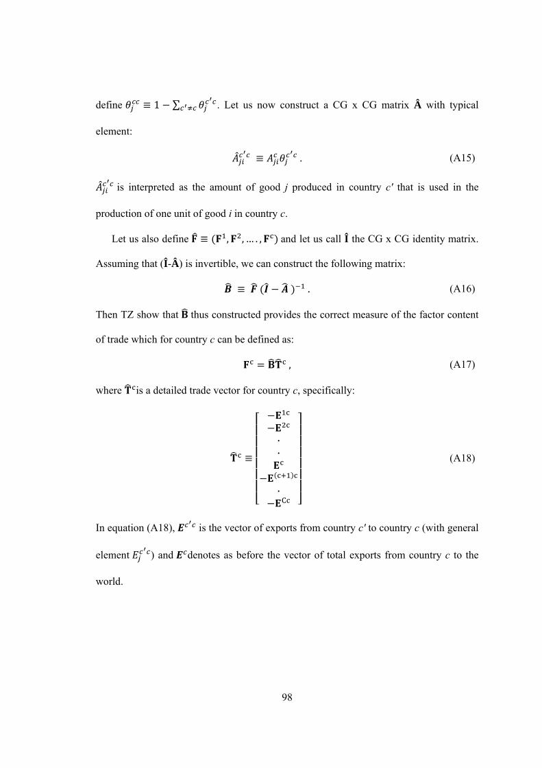
98

define 1 ∑ . Let us now construct a CG x CG matrix Â with typical

element:

. (A15)

is interpreted as the amount of good j produced in country cʹ that is used in the

production of one unit of good i in country c.

Let us also define , , … . , and let us call Î the CG x CG identity matrix.

Assuming that (Î-Â) is invertible, we can construct the following matrix:

. (A16)

Then TZ show that thus constructed provides the correct measure of the factor content

of trade which for country c can be defined as:

, (A17)

where is a detailed trade vector for country c, specifically:

··

·C

(A18)

In equation (A18), is the vector of exports from country cʹ to country c (with general

element ) and denotes as before the vector of total exports from country c to the

world.

99

The interpretation of this procedure is as follows. 56 As already suggested by

Deardorff (1982) and calculated in a somewhat more restricted sense by Reimer (2006),

this procedure keeps track of not only where each intermediate input is produced, but also

where its intermediate inputs are produced, and so on. It then correctly calculates the

factor content of production by using the techniques of production where each input was

produced. Note that the element (equation A15) generalizes , which is the relevant

measure when we do not need to keep track where each intermediate input is produced.

When is that the case? Either when there are no traded inputs (a dubious hypothesis) or

when all countries produce with the same techniques of production (our null hypothesis

along the demand dimension). One difficulty is that is not provided by the available

data sets, and only is. To get around this problem, TZ use a proportionality argument,

namely they assume that if, say, 1% of good j’s absorption in country c is due to imports

from country cʹ (that is, 0.01), then all industries will use 1% of good j from

country cʹ, in whatever their needs are for good j. This is in essence what underlies

equation (A15). Accepting this construction of matrix Â, equation (A16) provides the

total factor input in a global way, in the same sense that equation (A11) provided the total

factor input for each country separately. This is what finally allows the calculation of the

factor content of trade (equation A17), keeping track of imports from each individual

country, and the exports of country c (definition A18).

56 We are quite terse in this paragraph, as we are essentially repeating TZ, to which the reader is directed for an ampler discussion.

100

B. For Chapter Three

The data in this chapter came from the Input-Output (IO) tables and Structural

Analysis (STAN) database of the OECD in 1985. All of the data in this chapter are given

by Davis and Weinstein (2001a), except the matrix of trade costs in factor services. This

data section explains briefly where Davis and Weinstein got their original data, and how

we obtain trade costs.

B1. Data Sources:

The data for the total factor requirement matrix (B) used the 1985 OECD IO tables.

The data for capital (K) and labor (L) used the 1997 OECD STAN database for

manufacturing sectors and the 1996 International Sectoral Database (ISDB) for other

sectors. Capital stock was calculated by the perpetual inventory method.57 Sectoral labor

inputs and total employment for the year 1985 were derived from the OECD STAN

databases and the ISDB. Labor for manufacturing sectors data were taken from the STAN

Numbered Engaged (NE) and, for non-manufacturing sectors of labor, the ISDB Total

Employment was used.

The data for production ( ), demand , and trade , , used the 1995

OECD IO database. The vector of factor endowments ( for country c was calculated

as: . The data for trade costs ( were taken from Bernard, Jensen, and

Schott’s (2006) data and were modified for this chapter.

57 “The Perpetual Inventory Method (PIM) generates an estimate of the capital stock by accumulating past purchases of assets over their estimated service lives” (Measuring Capital, OECD Manual (2001), p.43).

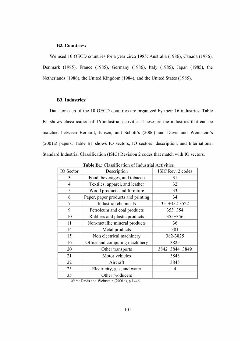
101

B2. Countries:

We used 10 OECD countries for a year circa 1985: Australia (1986), Canada (1986),

Denmark (1985), France (1985), Germany (1986), Italy (1985), Japan (1985), the

Netherlands (1986), the United Kingdom (1984), and the United States (1985).

B3. Industries:

Data for each of the 10 OECD countries are organized by their 16 industries. Table

B1 shows classification of 16 industrial activities. These are the industries that can be

matched between Bernard, Jensen, and Schott’s (2006) and Davis and Weinstein’s

(2001a) papers. Table B1 shows IO sectors, IO sectors’ description, and International

Standard Industrial Classification (ISIC) Revision 2 codes that match with IO sectors.

Table B1: Classification of Industrial Activities IO Sector Description ISIC Rev. 2 codes

3 Food, beverages, and tobacco 31 4 Textiles, apparel, and leather 32 5 Wood products and furniture 33 6 Paper, paper products and printing 34 7 Industrial chemicals 351+352-3522 9 Petroleum and coal products 353+354

10 Rubbers and plastic products 355+356 11 Non-metallic mineral products 36 14 Metal products 381 15 Non electrical machinery 382-3825 16 Office and computing machinery 3825

20 Other transports 3842+3844+3849

21 Motor vehicles 3843 22 Aircraft 3845 25 Electricity, gas, and water 4 35 Other producers

Note: Davis and Weinstein (2001a), p.1446.

102

B4. Trade Costs:

Along with Davis and Weinstein’s (2001a) data, this chapter also uses trade costs data

from 1987. Because we cannot get data for trade costs from 1985, we assume that trade

costs in 1987 were approximately similar to the trade costs in 1985.

We explained Bernard et al.’s (2006) paper in the section I of this chapter, and

explained how they calculated the trade costs. With their explanation, we are going to

expand our explanation here to show how we use and calculate our trade costs data for

the purpose of this chapter.

Bernard et al. (2006) create a dataset of industry level trade costs for years, 1982,

1987, and 1992. They calculate industry-level data and construct ad valorem trade costs.

These ad valorem trade costs data are changed by time and across industries. Bernard et

al. (2006) define the trade costs variable for industry i and year t as, .

are the sum of the ad valorem duty( ) and the ad valorem freight and

insurance ( ). Bernard et al. calculate and from Feenstra (2006). They define the

trade costs rate for industry i as the weighted average of trade cost rates across all

products in industry i. Bernard et al. (2006) explain tariff, freight, and total trade costs.

We now explain how to calculate trade costs, C for this chapter. To calculate trade

costs for industry i for the United States, we used Bernard et al.’s (2006) data. First, we

harmonized the two-digit SIC industry in Bernard et al.’s trade cost rates and the ISIC

Rev.2 codes in Davis and Weinstein’s paper.

When two or more industries (i, j) in Bernard et al.’s data correspond to only one of

Davis and Weinstein’s IO industries, we used the following equation:

. (B1)

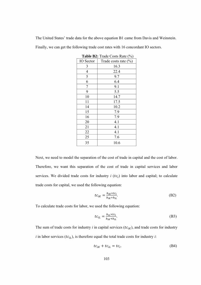
103

The United States’ trade data for the above equation B1 came from Davis and Weinstein.

Finally, we can get the following trade cost rates with 16 concordant IO sectors.

Table B2: Trade Costs Rate (%) IO Sector Trade costs rate (%)

3 16.3

4 22.4

5 9.7

6 6.4

7 9.1

9 5.5

10 14.7

11 17.5

14 10.2

15 7.9

16 7.9

20 4.1

21 4.1

22 4.1

25 7.6

35 10.6

Next, we need to model the separation of the cost of trade in capital and the cost of labor.

Therefore, we want this separation of the cost of trade in capital services and labor

services. We divided trade costs for industry i ( ) into labor and capital; to calculate

trade costs for capital, we used the following equation:

. (B2)

To calculate trade costs for labor, we used the following equation:

. (B3)

The sum of trade costs for industry i in capital services ( ), and trade costs for industry

i in labor services ( ), is therefore equal the total trade costs for industry i:

. (B4)

104

Furthermore, we have assumed that the division of trade costs into labor and capital

services has followed the same proportion as production in the same industry. This is

obviously a very strong assumption, but it is one that is dictated by the data.

105

REFERENCES

Aït-Sahalia, Yacine, Jonathan A. Parker, and Motohiro Yogo (2004) “Luxury Goods and the Equity Premium,” Journal of Finance, 59(6), 2959-3004. Anderson, James E. and Eric van Wincoop (2002) “Borders, Trade and Welfare,” in Brookings Trade Forum 2001. Susan Collins and Dani Rodrik, eds. Washington: Brookings Institution, 207-244. Anderson, James E. and Eric van Wincoop (2004) “Trade Costs,” Journal of Economic Literature, 42(3), 691-751. Andrews, Donald W.K. (1993) “Tests for Parameter Instability and Structural Change with Unknown Change Point,” Econometrica, 61 (4), 821-856.

Andrews, Donald W.K. (2003) “Tests for Parameter Instability and Structural Change with Unknown Change Point: a Corrigendum,” Econometrica, 71 (1), 395-397. Barroso, José Manuel (2007) “Hands across the ocean,” The International Herald Tribune Wednesday, April 25. Bergstrand, Jeffery and Peter Egger (2004) "Trade Costs and Intra-Industry Trade," University of Notre Dame, 1-19. Bergstrand Jeffery and Peter Egger (2006) "Trade Costs and Intra-Industry Trade," Review of World Economics/Blackwell, 142, July (3rd Quarter/Summer), 433-458. Bernard, Andrew, Bradford Jensen, and Peter Schott (2006) “Trade Costs, firms and productivity,” Journal of Monetary Economics, 53, 917-937. Bowen, Harry, Abraham Hollander, and Jean-Marie Viaene (1998) “Applied International Trade Analysis,” Ann Arbor, The University of Michigan Press. Bowen, Harry P., Edward E. Leamer, and Leo Svikauskas (1987) “Multi-country,Multi- factor Tests of the Factor Abundance Theory,” The American Economic Review, 77(5), 791-809. Brecher, R.A. and E.U. Choudri (1986) “The factor content of consumption in Canada and the United States: A two country test of the Heckscher-Ohlin-Vanek model,” Paper presented at the NBER Conference on Empirical Methods for International Trade, Cambridge, MA. Choi, Yong-Seok and Pravin Krishna (2004) "The Factor Content of Bilateral Trade: An Empirical Test," Journal of Political Economy, University of Chicago Press, 112(4), 887- 914.

106

Chung, Chul (2005) “Factor Content of Trade: Nonhomothetic Preferences and ‘Missing Trade’” Georgia Institute of Technology manuscript. Dalgin, Muhammed, Vitor Trindade, and Devashish Mitra (2008) “Inequality, Nonhomothetic Preferences and Trade: a Gravity Approach,” Southern Economic Journal, 74(3), 747-774. Davis, D.R. (1997) Critical Evidence on Comparative Advantage? North-North Trade in a Multilateral World, Journal of Political Economy, 105(5), 1051-1060. Davis, Donald (1998) "The Home Market Effect, Trade and Industrial Structure," The American Economic Reviews, 88(5), 1264-1276. Davis, D. R. and D.E. Weinstein (2001a) “An Account of Global Factor Trade,” The American Economic Review, 91(5), 1423-1453. Davis, D. R. and D.E. Weinstein (2001b) “The Factor Content of Trade,” NBER working paper 8637. Deardorff, Alan V. (1982) “The General Validity of the Heckscher-Ohlin Theorem,” The American Economic Review, 72 (4), 683-694. Deardorff, A. V. (1998) Determinants of Bilateral Trade: Does Gravity work in a Neoclassical World? in: Frankel, J.A.(Ed.), The Regionalization of the World Economy, University of Chicago Press. Deardorff, Alan V. (2004) “Local Comparative Advantage: Trade Costs and the Pattern of Trade,” University of Michigan Research Seminar in International Economics Working paper No. 500. Deaton, Angus (1992) Understanding Consumption. New York: Oxford University Press. Debaere, Peter (2005) “Monopolistic Competition and Trade, revisited: Testing the Model without Testing for Gravity,” Journal of International Economics, 66, 249-266. Debaere, Peter (2003) “Relative Factor Abundance and Trade,” Journal of Political Economy, 111(3), 589-610. Dinopoulos, Elias, Kenji Fujiwara, and Koji Shimomura (2007) “International Trade and Volume Pattern under Quasi-Linear Preferences,” University of Florida manuscript. Dixit, A.K. and V. Norman (1980) Theory of International Trade, Cambridge, Nisbet/Cambridge University Press, Cambridge. Dollar, D. (1993) “Technology Differences as a Source of Comparative Advantage,” The American Economic Review, 83, 431-435.

107

Ethier, Wilfred J. (1982) “National and International Returns to Scale in the Modern Theory of International Trade,” The American Economic Review, 72, 950-959. Feenstra, Robert C. (1996) “U.S. Imports, 1972-1994. Data and Concordances,” NBER Working paper 5515. Feenstra, Robert C. (2003) Advanced International Trade, Princeton University Press. Feenstra, Robert C., et al. (2002) “U.S. Imports, Exports and Tariff data, 1989-2001,” NBER working paper 9387, December. Feenstra, Robert C., website available at http://cid.econ.ucdavis.edu/. Francois, Joseph F. and Seth Kaplan (1996) “Aggregate Demand Shifts, Income Distribution, and the Linder Hypothesis,” Review of Economics and Statistics, 78 (2), 244-250. Gabaix, Xaiver (1997) “The Factor Content of Trade: A Rejection of the Heckscher- Ohlin Leontief Hypothesis,” Working paper, Harvard University, May. Hakura, Dalia (1995) “A Test of the General Validity of the Heckscher-Ohlin Theorem for Trade in the European Community,” Three Essays on the Effects of International Trade, Unpublished dissertation, University of Michigan. Hakura, D. (2001) “hy does HOV fail? The role of technological differences within the EC,” Journal of International Economics, 54, 361-382. Hamiton, D. S. and Quinlan, J. P. (2004) “Partners in Prosperity: The changing Geography of the Transatlantic Economy,” Center for Transatlantic Relations. Harrigan, J (1997) “Technology, Factor Supplies, and International Specialization: Estimating the Neoclassical Model,” The American Economic Review, 87(4), 475-494. Helpman, Elhanan (1987) “Imperfect Competition and International Trade: Evidence from Fourteen Industrial Countries,” Journal of the Japanese and International Economies, I, 62-81. Helpman, Elhanan (1984) “The Factor Content of Foreign Trade,” Economic Journal, 94 (373), 84-94. Hunter, Linda C. (1991) “The Contribution of Nonhomothetic Preferences to Trade,” Journal of International Economics 30, 345-358. Hunter, Linda C. and James R. Markusen (1988) “Per-Capita Income as a Determinant of Trade,” in Robert C. Feenstra, ed., Empirical Methods for International Trade,

108

Cambridge, MA: MIT Press. Hummels, David and J. Levinsohn (1995) “Monopolistic Competition and International Trade: Reconsidering the Evidence,” The Quarterly Journal of Economics, 110, 799-836. Hummels, David and Volodymyr Lugovskyy (2006) “Are Matched Partner Trade Statistics a Usable Measure of Transportation Costs?” Review of International Economics, 14(1), February. Hummels, David (2001a) “Time as a Trade Barriers,” manuscript, Purdue University. Hummels, David (2001b) “Toward a Geography of Trade Costs,” manuscript, Purdue University. Jacks, David, Christopher Meissner, and Dennis Novy (2008) “Trade Costs, 1870-2000,” The American Economic Review, 98(2), 529-534. Johnson, Harry G. (1959) “International Trade, Income Distribution, and the Offer Curve,” Manchester School of Economic and Social Studies, 27, 241-260. Korth, Christopher (1987) “International Counter Trade,” Quorum Books. Lai, Huiwen and Susan Chun Zhu (2007) “Technology, Endowments, and the Factor Content of Bilateral Trade,” Journal of International Economics, 71, 389-409. Leamer, Edward E. (1980) “The Leontief Paradox, Reconsidered,” Journal of Political Economy, 88(3), 495-503. Leamer, Edward E. and James Levinsohn (1995) “International Trade Theory: The Evidence,” Handbook of International Economics, Vol.3, Ch.26, 1339–1394, Edited by G. Grossman and K. Rogoff, Elsevier Science B.V. Leontief, Wassily W. (1953) “Domestic Production and Foreign Trade: The American Capital Position Re-Examined,” Proceedings of the American Philosophical Society, 97 (4), 332-349. Lai H. and S.C. Zhu (2004) “The determinant of bilateral trade,” Canadian Journal of Economics, 37(2), 459-483. Linder, Staffan (1961) An Essay on Trade and Transformation, Stokholm: Almqvist and Wicksell. Markusen, James R. (1986) “Explaining the Volume of Trade: an Eclectic Approach,” The American Economic Review, 76(5), 1002-1011. Matsuyama, Kiminori (2000) “A Ricardian Model with a Continuum of Goods under

109

Nonhomothetic Preferences: Demand Complementarities, Income Distribution, and North-South Trade,” Journal of Political Economy, 108, 1093-1120. Miller, Ronald E. and Peter D. Blair (1985) Input-Output Analysis: Foundations and Extensions, Englewood Cliffs, New Jersey: Prentice-Hall. Mitra, D. and Trindade, V. (2005) “Inequality and Trade,” Canadian Journal of Economics, 38(4), 1253-1271. Muhammed, Dalgin, Devashish Mitra, Vitor Trindade (2008) “Inequality, Non- homothetic Preferences, and Trade: A Gravity Approach,” Southern Economic Journal, 74(3), 747-774. Obstfeld, Maurice and Kenneth Rogoff. (2000) "The Six Major Puzzles in International Macroeconomics. Is There a Common Cause?" in NBER Macroeconomics Annual 2000, B.S. Bernanke and K. Rogoff, eds. Cambridge, MA: MIT Press, 339-390. OECD (Organization of Economic Cooperation and Development) (2002) “The OECD Input–Output Database, International Sectoral Data Base, and The OECD Structural Analysis (STAN) Data Base,” OECD Economic and Statistic Division. OECD (2005) “The OECD STAN database for Industrial Analysis,” available at http://www.oecd.org/dataoecd/53/21/34464010.doc. Ogaki, Masao and Carmen M. Reinhart (1998) “Measuring Intertemporal Substitution: The Role of Durable Goods,” Journal of Political Economy, 106(5), 1078-1098. Okubo, Masakatsu (2008) “Intertemporal Substitution and Nonhomothetic Preferences,” Economics Letters, 98, 41-47. Ostapik E. and Kei-Mu Yi (2007) “International Trade: Why we don’t have more of it,” Business Review, Q3. Penn World Table 6.2, University of Pennsylvania. Prebisch, R. (1964) “Towards a new trade policy for development,” Report by the Secretary General of UNCTAD, United Nations, New York. Radelet, Steven and Jeffrey Sachs (1998) “Shipping Costs, Manufactured Exports, and Economic Growth,” January. Ramezzana, Paolo (2002) “Per Capita Income and Industrial Demand in Economic Development and International Trade,” University of Virginia manuscript. Ray, Edward (1981a) “Tariff and Non-tariff Barriers to Trade in the United States and Abroad,” The Review of Economics and Statistics, 63(2), 161-168.

110

Ray, Edward (1981b) “The determinants of Tariffs and Nontariff Trade Restrictions in the U.S.,” Journal of Political Economy, 89, 105-121. Reimer, Jeffrey J. (2006) “Global Production Sharing and Trade in Services of Factors,” Journal of International Economics, 68, 384-408. Reimer, Jeffrey J. and Thomas W. Hertel (2007) “Non-homothetic Preferences and International Trade,” Oregon State University manuscript. Samuelson, Paul A. (1952) “The Transfer problem and Transport Costs,” Economic Journal, 62(246), 278-304. Schott, Peter K. (2003) “One Size Fits All? Heckscher-Ohlin Specialization in Global Production,” The American Economic Review, 93(3), 686-708. Schott, P., website available at www.som.yale.edu/faculty/pks4/sub_international.htm. Schott, P., “Falling Trade Costs, Heterogeneous Firms and Industry Dynamics,” Yale School of Management, Mimeo. Singer, H. (1950) “The distributions of gains between investing and borrowing countries,” The American Economic Review, Vol.40. Staiger, R. W., Alan V. Deardorff, and Robert M. Stern (1987) “An Evaluation of Factor Endowments and Protection as Determinants of Japanese and American Foreign Trade,” The Canadian Journal of Economics, 20(3), 449-463. Tchamourliyski, Yuriy (2002) “Distance and Bilateral Trade: the Role of Nonhomothetic Preferences,” Boston College manuscript. Thursby, Jerry G. and Marie C. Thursby (1987) “Bilateral Trade Flows, the Linder Hypothesis, and Exchange Risk,” The Review of Economics and Statistics, 69, 488-495. Trefler, Daniel (1993) “International Factor Price Differences: Leontief was Right!” Journal of Political Economy, 101 (6), 961-987. Trefler, Daniel (1995) “The Case of the Missing Trade and Other Mysteries,” The American Economic Review, 85, 1029-1046. Trefler, Daniel and Susan Chun Zhu (2000) “Beyond the Algebra of Explanation: HOV for the Technology Age,” The American Economic Review, 90(2), 145-149. Trefler, Daniel and Susan C. Zhu (2006) “The Structure of Factor Content Predictions,” University of Toronto manuscript.

111

United Nations (1968) Statistical Papers, Series M, No. 4, rev. 2, New York. Vanek, Jaroslav (1968) “The Factor Proportions Theory: The N-Factor Case,” Kyklos, 21(4), 749-754. World Development Indicators (2007) World Bank. Yamano, Norihiko and Nadim Ahmad (2006) The OECD Input-Output Database: 2006 Edition, STI Working paper no. 2006/8, OECD. Yanikkaya, Halit (2003) “Trade openness and economic growth: a cross-country empirical investigation,” Journal of Development Economics, 72, 57-89.

112

VITA

Yeon Joon Kim was born in South Korea on March 26, 1973. He received a

master’s degree in economics from State University of New York at Albany on

December 2003. In May 2009, he received a Ph. D. in Economics from the University of

Missouri-Columbia. He worked for the Ways and Means Committee in the New York

State Assembly in 2004. He also worked for the Legislative Budget Office, State of

Missouri as an Economist from 2008 to 2009. He has been married to Yun Hee Kim

since 2001 and has a daughter, Seo Yeon and a son, Joel.

Documents

THREE ESSAYS ON THE FACTOR CONTENT OF TRADE