Embed Size (px)
Citation preview
1
May 16, 2000Revised and re-submitted to IEEE Transactions on Robotics and Automation
Time Domain Passivity Control of Haptic Interfaces
Blake Hannaford
Department of Electrical EngineeringUniversity of Washington
Box 352500, Seattle, WA 98195-2500
Jee-Hwan Ryu
Department of Mechanical EngineeringKorea Advanced Institute of Science and Technology
Taejeon, 305-701, Korea
Abstract
A patent pending, energy based, method is presented for controlling a hapticinterface system to ensure stable contract under a wide variety of operating conditions.System stability is analyzed in terms of the time -- domain definition of passivity. Wedefine a "Passivity Observer" (PO) which measures energy flow in and out of one ormore subsystems in real-time software. Active behavior is indicated by a negative valueof the PO at any time.
We also define the "Passivity Controller" (PC), an adaptive dissipative elementwhich, at each time sample, absorbs exactly the net energy output (if any) measured bythe PO. The method is tested with simulation and implementation in the "Excalibur"haptic interface system. Totally stable operation was achieved under conditions such asstiffness > 100 N/mm or time delays of 15ms. The PO/PC method requires very littleadditional computation and does not require a dynamical model to be identified.
2
I. Introduction
One of the most significant problems in haptic interface design is to create a control
system which simultaneously is stable (i.e. does not exhibit vibration or divergent
behavior) and gives high fidelity under any operating conditions and for any virtual
environment parameters. A classic engineering trade off is presented since realism of the
haptic interface (for example in terms of stiffness of "hard" objects) must often be
reduced in order to guarantee totally stable operation. Initial efforts to solve this problem
introduced the "virtual coupling" between the virtual environment and the haptic device
(Colgate et al, 1995, Zilles and Salisbury, 1995). The virtual coupling is a virtual
mechanical system containing a combination of series and parallel elements interposed
between the haptic interface and the virtual environment to limit the maximum or
minimum impedance presented by the virtual environment in such a way as to guarantee
stability. Particulars of virtual coupling design depend the causality of the virtual
environment and the haptic device. By causality, we refer to the selection of velocity or
force as input and its complement (force or velocity) as output. Possible VE causalities
include impedance based (position/velocity input, force output), admittance based (force
input, position/velocity output), or constraint based (position input / position output). In
the case of an impedance based environment (typical of many implemented systems), a
virtual spring and damper in parallel are typically connected in series between the haptic
interface and the virtual environment. Stability in this case depends inversely on the
stiffness being rendered by the system and the series stiffness has the effect of setting the

3
maximum stiffness. Correct selection of the virtual coupling parameters will allow the
highest possible stiffness without introducing instability.
The virtual coupling parameters can be set empirically, but several previous research
projects have sought out a theoretical design procedure.
Interesting virtual environments are always non-linear and the dynamic properties of
a human operator are always involved. These factors make it difficult to analyze haptic
systems in terms of known parameters and linear control theory. One fruitful approach is
to use the idea of passivity to guarantee stable operation. Anderson and Spong (1992) and
Neimeyer and Slotine (1991) have used passivity ideas in the related area of stable
control of force-feedback teleoperation with time delay. Colgate and Schenkel (1994)
have used it to derive fixed parameter virtual couplings (i.e., haptic interface controllers).
Passivity is a sufficient condition for stability which has the following attractive
features:
• Uses intuitively attractive energy concepts: A system is passive if and only if
the energy flowing in exceeds the energy flowing out for all time.
• Allows a global stability conclusion to be drawn from considering system
blocks individually.
• Applies to linear and non-linear systems.
• Experience and some evidence (Hogan, 1989) shows that it is safe to assume
the human operator is passive at frequencies of interest.
The major problem with using passivity for design of haptic interaction systems is
that it is over conservative. In many cases performance can be poor if a fixed damping
value is used to guarantee passivity under all operating conditions.
4
Haptic interfaces share with force feedback teleoperator systems the interesting
property that information and energy flows in two directions through a single interface
between the human operator and the virtual or real environment. This property means that
ideas from the theory of electrical networks (or more generally the “general systems
theory” of H. Paynter, (1961)) can be applied to good effect (Hannaford, 1989, Neimeyer
and Slotine, 1991). The virtual coupling is one example of such a network.
Adams (Adams and Hannaford 1999b) derived a method of virtual coupling design
from two port network theory which applied to all causality combinations and was less
conservative than passivity based design. They were able to derive optimal virtual
coupling parameters using a dynamic model of the haptic device and by satisfying
Lewellyn's "absolute stability criterion", an inequality composed of terms in the two-port
description of the combined haptic interface and virtual coupling system. This procedure
guaranteed a stable and high performance virtual coupling as long as the virtual
environment was passive. Miller et. al. (Miller et al., 1999a, 1999b, 2000) has derived
another design procedure which extends the analysis to non-linear environments and
extracts a damping parameter to guarantee stable operation.
There are several mechanisms by which a VE or other part of the system might
exhibit active behavior even when it is designed to be passive. These include delays due
to numerical integration schemes, quantization (Colgate et al., 1995) and interactions
between the discrete time system and the continuous time device/human operator
(Colgate and Schenkel 1994). These contributing factors to instability have been termed
“energy leaks” by Gillespie and Cutkosky (1996).
5
Yokokohji et al. (2000) studied teleoperation in the presence of time delay. Their
control method had undesirable behavior in the case of sudden loss of the communication
link. They computed an on-line estimate of energy production/dissipation using wave
variables and used this estimate to disable system operation in the case of instability due
to link loss.
In this paper, we will develop analysis and control of instability in complex systems
such as haptic interfaces using the time domain definition of passivity (see below). We
define the "Passivity Observer," and the "Passivity Controller," and show how they can
be applied to haptic interfaces in place of fixed-parameter virtual couplings. We then
study properties of the controller through simulation and experimental evaluation in our
previously described Excalibur system (Adams et al., 1999a, 2000).
II. Definitions
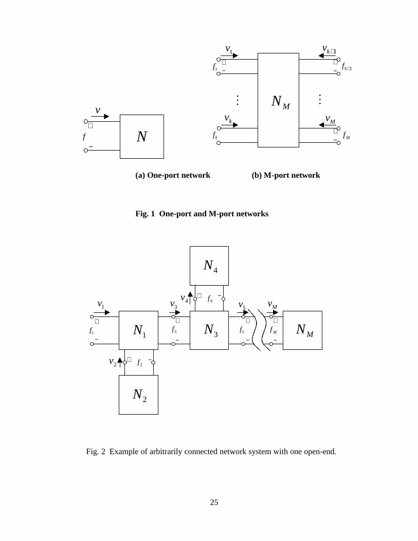
In this section we review passivity properties of networks and define our observer and
controller. First, we define the sign convention for all forces and velocities so that their
product is positive when power enters the system port (Fig. 1). We also assume that the
system has initial stored energy at t = 0 of E(0).
We then use the following widely known definitions of passivity.
Definition 1: The one-port network, N , with initial energy storage ( )0E is passive if
and only if,
( ) ( ) ( ) 0 ,000
≥∀≥+∫ tEdvft
τττ (1)
for admissible force ( )f and velocity ( )v .
6
Equation (1) states that the energy supplied to a passive network must be greater than
negative E(0) for all time (a. J. van der Schaft 2000, Adams and Hannaford 1999b,
Desoer and Vidyasagar 1975, J. C. Willems 1972).
Definition 2: The M-port network, NM, with initial energy storage ( )0E is passive if
and only if,
( ) ( ) ( ) ( )( ) ( ) 0 ,000 11 ≥∀≥+++∫ tEdvfvft
MM τττττ L (2)
for all admissible forces ( )Mff ,,1 L and velocities ( )Mvv ,,1 L .
The elements of a typical haptic interface system include the virtual environment, the
virtual coupling network, the haptic device controller, the haptic device, and the human
operator. Many of the input and output variables of these elements of haptic interface
systems can be measured by the computer and (1) and (2) can be computed in real time
by appropriate software. This software is very simple in principle because at each time
step, (1) or (2) can be evaluated with few mathematical operations.
A. Passivity Observer
The conjugate variables which define power flow in such a computer system are
discrete-time values. We confine our analysis to systems having sampling rate
substantially faster than the dynamics of the haptic device, human operator, and virtual
environment so that the change in force and velocity with each sample is small. Many
haptic interface systems (including our own, sec. V.) having sampling rates of 1000 Hz,
more than ten times the highest significant mode in our system. Thus, we can easily
7
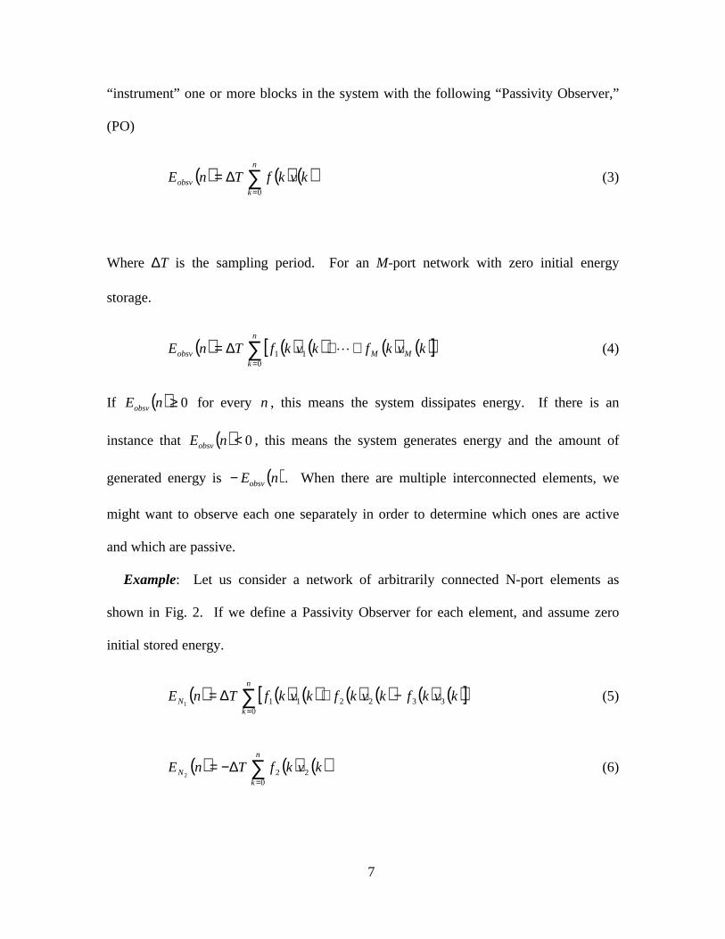
“instrument” one or more blocks in the system with the following “Passivity Observer,”
(PO)
( ) ( ) ( )∑=
∆=n
kobsv kvkfTnE
0
(3)
Where ∆T is the sampling period. For an M-port network with zero initial energy
storage.
( ) ( ) ( ) ( ) ( )[ ]∑=
++∆=n
kMMobsv kvkfkvkfTnE
011 L (4)
If ( ) 0≥nEobsv for every n , this means the system dissipates energy. If there is an
instance that ( ) 0<nEobsv , this means the system generates energy and the amount of
generated energy is ( )nEobsv− . When there are multiple interconnected elements, we
might want to observe each one separately in order to determine which ones are active
and which are passive.
Example: Let us consider a network of arbitrarily connected N-port elements as
shown in Fig. 2. If we define a Passivity Observer for each element, and assume zero
initial stored energy.
( ) ( ) ( ) ( ) ( ) ( ) ( )[ ]∑=
−+∆=n
kN kvkfkvkfkvkfTnE
0332211
1(5)
( ) ( ) ( )∑=
∆−=n
kN kvkfTnE
022
2(6)
8
( ) ( ) ( ) ( ) ( ) ( ) ( )[ ]∑=
−−∆=n
kN kvkfkvkfkvkfTnE
0554433
3(7)
( ) ( ) ( )∑=
∆=n
kN kvkfTnE
044
4(8)
( ) ( ) ( )∑=
∆=n
kMMN kvkfTnE
M0
(9)
Total energy ( ) ( ) ( ) ( ) ( ) ( )nEnEnEnEnEnEMNNNNNobsv +++++= L
4321(10)
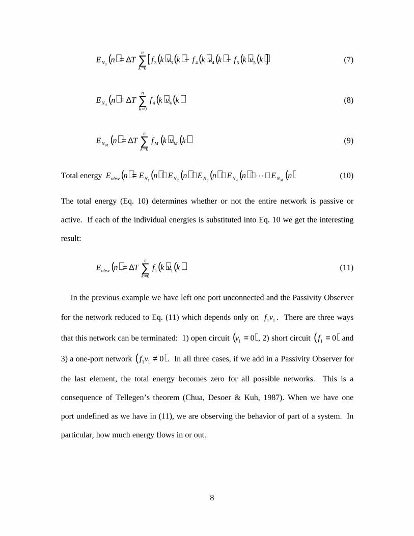
The total energy (Eq. 10) determines whether or not the entire network is passive or
active. If each of the individual energies is substituted into Eq. 10 we get the interesting
result:
( ) ( ) ( )∑=
∆=n
kobsv kvkfTnE
011 (11)
In the previous example we have left one port unconnected and the Passivity Observer
for the network reduced to Eq. (11) which depends only on 11vf . There are three ways
that this network can be terminated: 1) open circuit ( )01 =v , 2) short circuit ( )01 =f and
3) a one-port network ( )011 ≠vf . In all three cases, if we add in a Passivity Observer for
the last element, the total energy becomes zero for all possible networks. This is a
consequence of Tellegen’s theorem (Chua, Desoer & Kuh, 1987). When we have one
port undefined as we have in (11), we are observing the behavior of part of a system. In
particular, how much energy flows in or out.
9
We will refer to a port as “open-ended” when it is connected as in “3)” above, but the
analysis stops at that point. We then can restate the definition of passivity in the context
of a M-port system with multiple subcomponents.
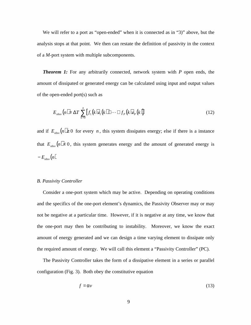
Theorem 1: For any arbitrarily connected, network system with P open ends, the
amount of dissipated or generated energy can be calculated using input and output values
of the open-ended port(s) such as
( ) ( ) ( ) ( ) ( )[ ]∑=
++∆=n
kPPobsv kvkfkvkfTnE
011 L (12)
and if ( ) 0≥nEobsv for every n , this system dissipates energy; else if there is a instance
that ( ) 0<nEobsv , this system generates energy and the amount of generated energy is
( )nEobsv−
B. Passivity Controller
Consider a one-port system which may be active. Depending on operating conditions
and the specifics of the one-port element’s dynamics, the Passivity Observer may or may
not be negative at a particular time. However, if it is negative at any time, we know that
the one-port may then be contributing to instability. Moreover, we know the exact
amount of energy generated and we can design a time varying element to dissipate only
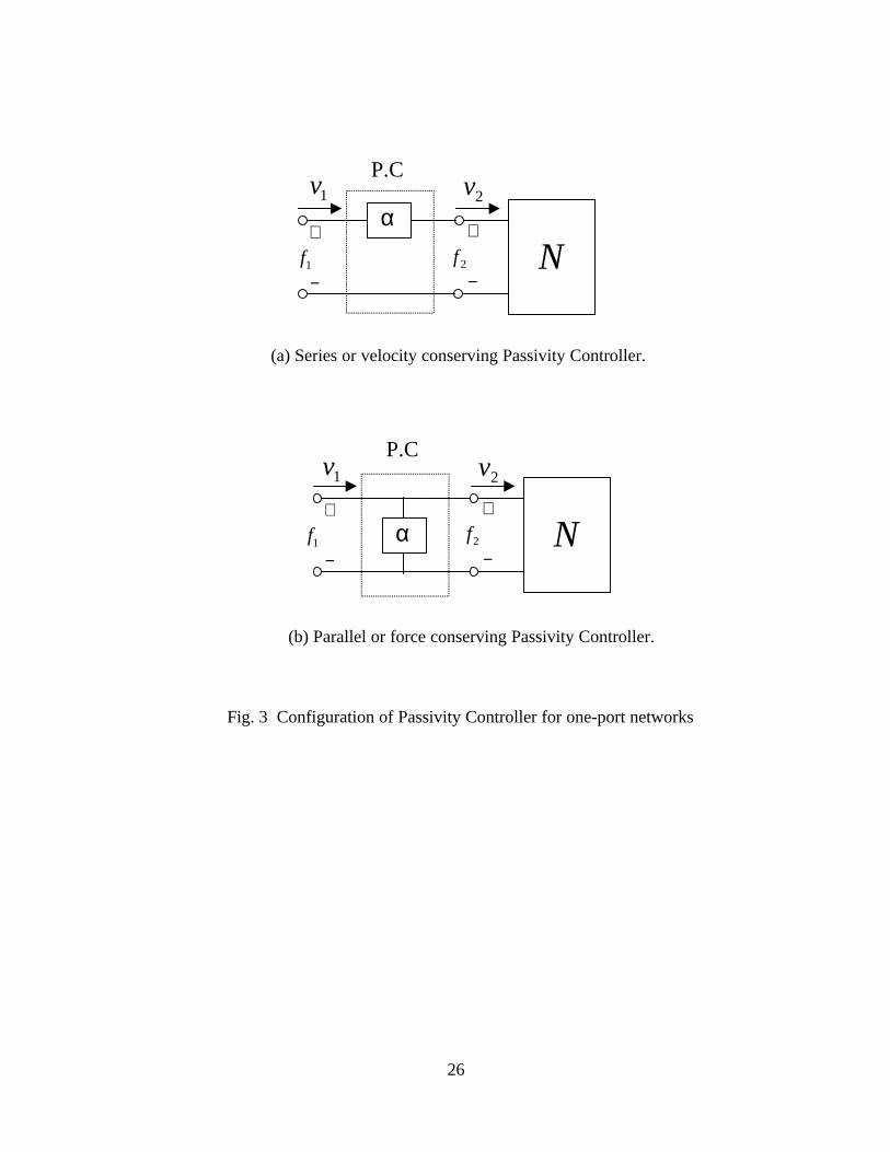
the required amount of energy. We will call this element a “Passivity Controller” (PC).
The Passivity Controller takes the form of a dissipative element in a series or parallel
configuration (Fig. 3). Both obey the constitutive equation
vf α= (13)
10
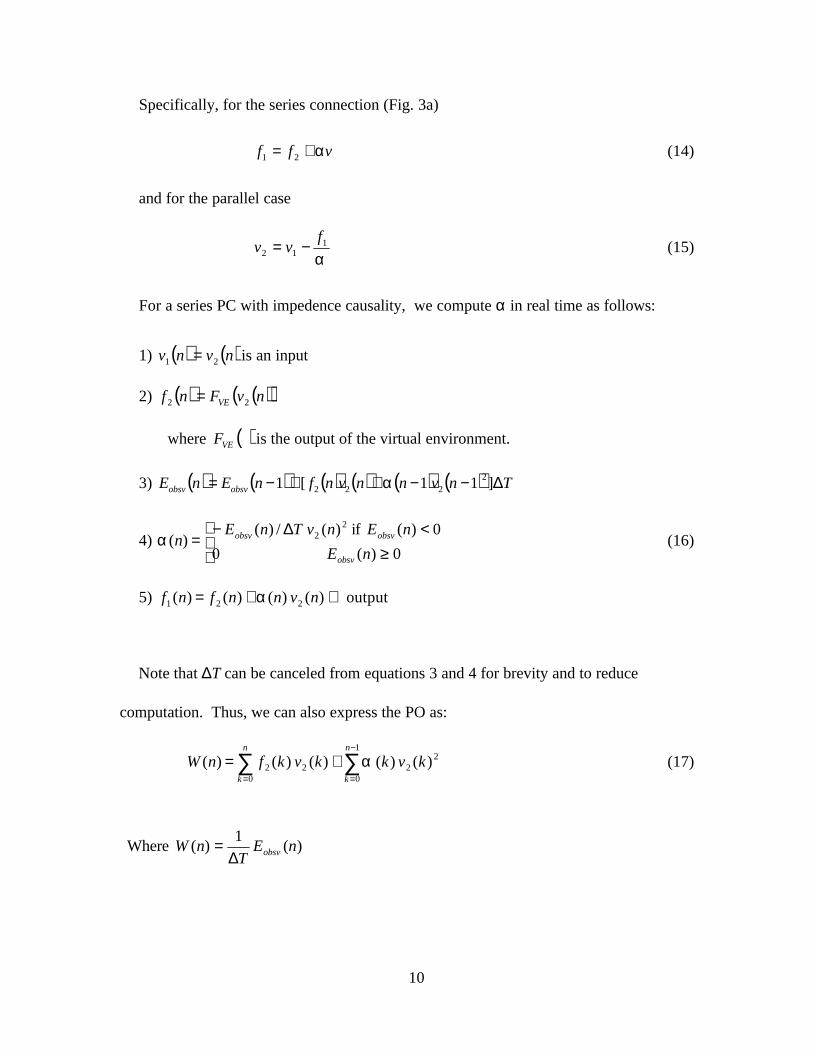
Specifically, for the series connection (Fig. 3a)
vff α+= 21 (14)
and for the parallel case
α1
12
fvv −= (15)
For a series PC with impedence causality, we compute α in real time as follows:
1) ( ) ( )nvnv 21 = is an input
2) ( ) ( )( )nvFnf VE 22 =
where ( )VEF is the output of the virtual environment.
3) ( ) ( ) ( ) ( ) ( ) ( ) TnvnnvnfnEnE obsvobsv ∆−−++−= ]11[1 2222 α
4)
≥<∆−
=0)( 0
0)( if )( /)( )(
22
nE
nEnvTnEn
obsv
obsvobsvα (16)
5) output )( )()( )( 221 ⇒+= nvnnfnf α
Note that ∆T can be canceled from equations 3 and 4 for brevity and to reduce
computation. Thus, we can also express the PO as:
22
1
02
02 )( )( )( )( )( kvkkvkfnW
n
k
n
k∑∑
−
==
+= α (17)
)(1
)( Where nET
nW obsv∆=
11
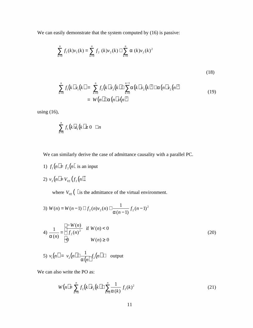
We can easily demonstrate that the system computed by (16) is passive:
(18)
( ) ( ) ( ) ( ) ( ) ( ) ( ) ( )
( ) ( ) ( )2
22
1
0
222
0 0211
n vnn W
n vnk vkk vkf k vkfn
k
n
k
n
k
α
αα
+=
++= ∑∑ ∑−
== = (19)
using (16),
( ) ( ) nkvkfn
k
∀≥∑=
00
11
We can similarly derive the case of admittance causality with a parallel PC.
1) ( ) ( )nfnf 21 = is an input
2) ( ) ( )( )nfVnv VE 22 =
where ( )VEV is the admittance of the virtual environment.
3) 2222 )1(
)1(
1)()()1()( −
−++−= nf
nnvnfnWnW
α
4)
≥
<−=
0)( 0
0)( if )(
)(
)(
1 22
nW
nWnf
nW
nα(20)
5) ( ) ( ) ( ) ( ) output 1
221 nfn
n v nv ⇒+=α
We can also write the PO as:
( ) ( ) ( ) 22
02
02 )(
)(
1kf
kk vkfnW
n
k
n
k∑∑
==+=
α(21)
∑∑∑===
+=n
k
n
k
n
k
kvkkvkfkvkf0
222
021
01 )()( )()( )()( α
12
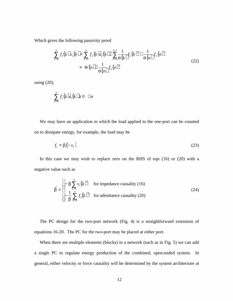
Which gives the following passivity proof
( ) ( ) ( ) ( ) ( ) ( ) ( ) ( )
( ) ( ) ( )22
22
22
1
02
021
01
1
11
n fn
n W
n fn
k fk
kvkfk vkfn
k
n
k
n
k
α
αα
+=
++= ∑∑∑−
=== (22)
using (20),
( ) ( ) nkvkfn
k
∀≥∑=
00
11
We may have an application in which the load applied to the one-port can be counted
on to dissipate energy, for example, the load may be
( )11 vf −= β (23)
In this case we may wish to replace zero on the RHS of eqn (16) or (20) with a
negative value such as
( )
( )
−
−=
∑
∑
=
=
(20)causality admittancefor 1
(16)causality impedancefor ˆ
0
21
0
21
n
k
n
k
kf
kv
β
ββ (24)
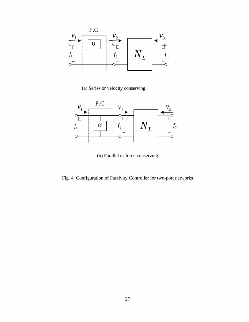
The PC design for the two-port network (Fig. 4) is a straightforward extension of
equations 16-20. The PC for the two-port may be placed at either port.
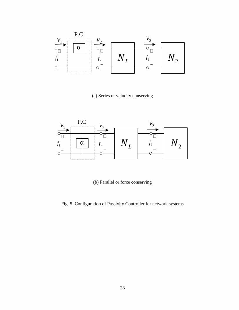
When there are multiple elements (blocks) in a network (such as in Fig. 5) we can add
a single PC to regulate energy production of the combined, open-ended system. In
general, either velocity or force causality will be determined by the system architecture at

13
the input port. As with the one-port, the causality determines whether a series or shunt
PC is used. The PC should be placed at the input port in the selected configuration.
Then, the system can be treated exactly as with the one-port element:
1) Solve the network to obtain the output variable (force for impedance causality,
velocity for admittance).
2) Update the Passivity Observer and compute the Passivity Controller according to (Eq.
16 or 20).
3) Compute and return the modified output variable.
III. Potential Problems
We have described two implementations of the Passivity Controller, the series
(velocity conserving) and parallel (force conserving) controllers. In the next paragraph
we suggest some performance limitations and issues that arise in the series Passivity
Controller. The same issues arise in dual form in the parallel controller, but these will not
be described in detail to save space.
A potential problem which may occur with the series Passivity Controller is that the
forces required to dissipate the generated energy may exceed the actuator limits. This is
especially true if velocity happens to be small. A related problem is that due to the well
known difficulties of computing a noise free velocity signal, we might want to limit the
value of α to avoid “magnifying noise”. For these reasons, we may want to limit the
magnitude of the force generated by the series Passivity Controller, limit the maximum
value of α, or both. In this case, the Passivity Controller may not be able to dissipate all
14
of the energy supplied by a subnetwork in one sample time. The excess energy must be
stored in the system for the next sample time. We explore this issue in the experimental
section below.
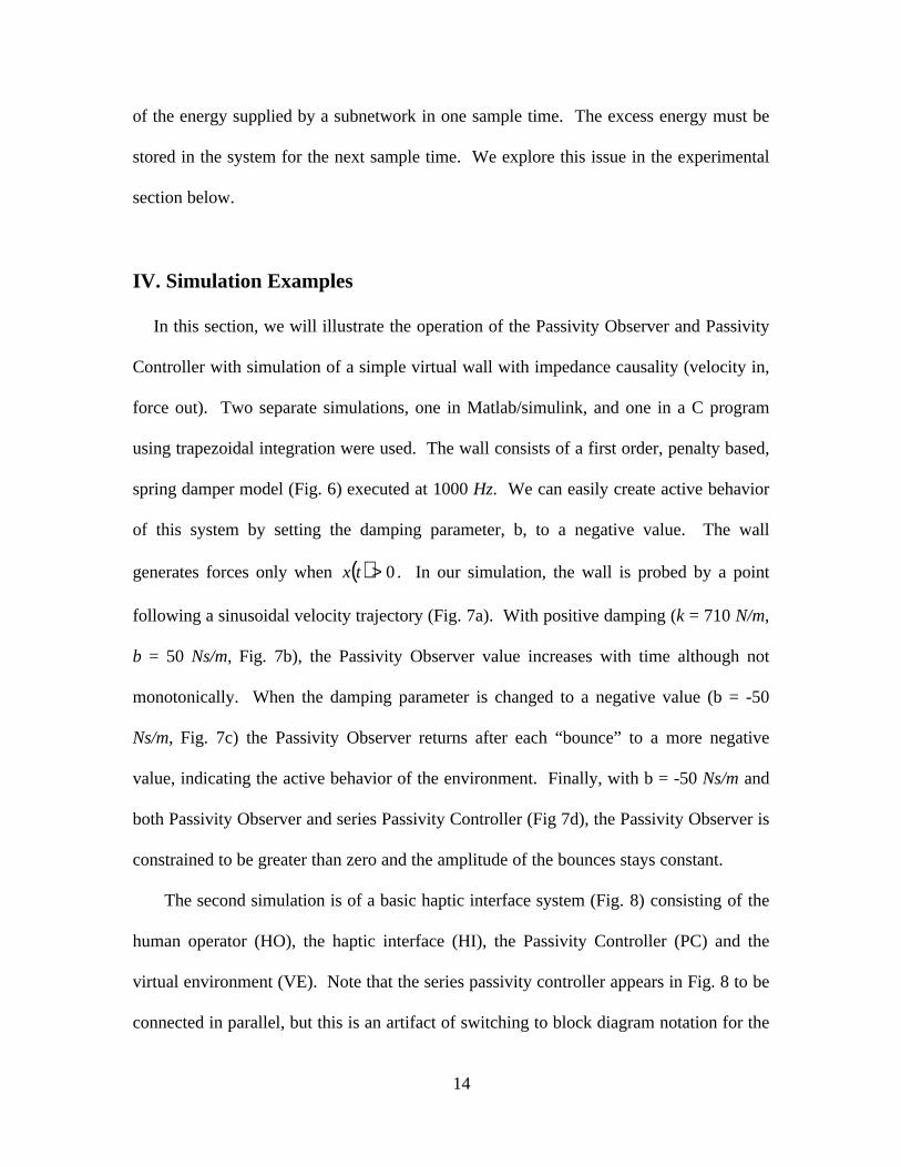
IV. Simulation Examples
In this section, we will illustrate the operation of the Passivity Observer and Passivity
Controller with simulation of a simple virtual wall with impedance causality (velocity in,
force out). Two separate simulations, one in Matlab/simulink, and one in a C program
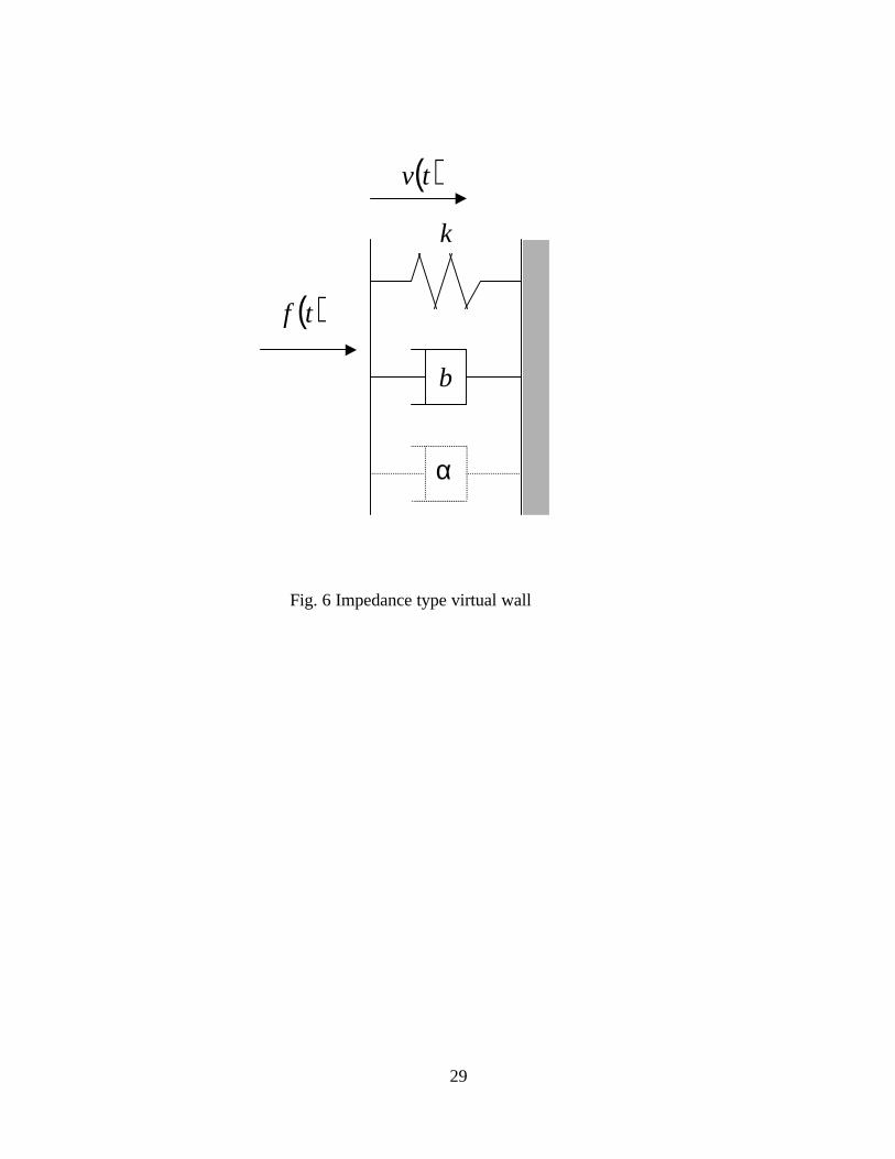
using trapezoidal integration were used. The wall consists of a first order, penalty based,
spring damper model (Fig. 6) executed at 1000 Hz. We can easily create active behavior
of this system by setting the damping parameter, b, to a negative value. The wall
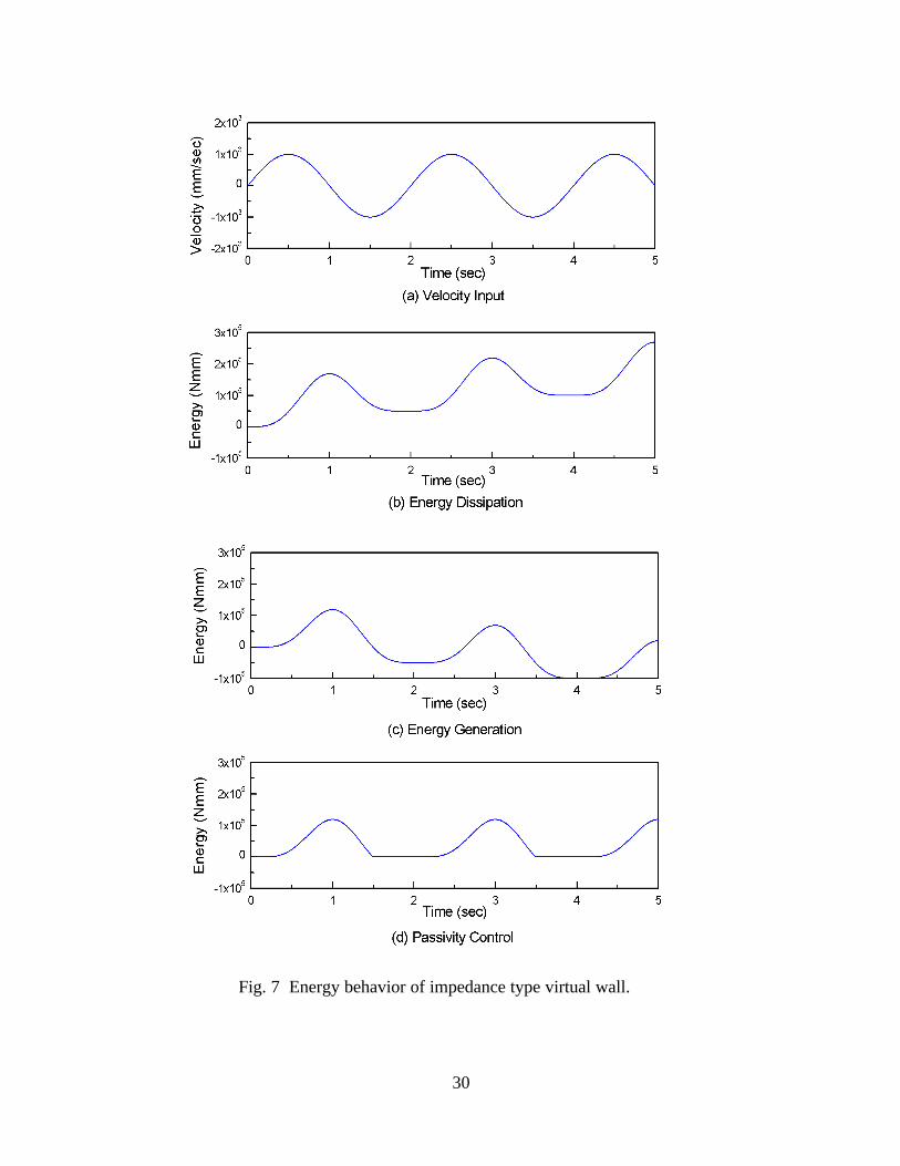
generates forces only when ( ) 0>tx . In our simulation, the wall is probed by a point
following a sinusoidal velocity trajectory (Fig. 7a). With positive damping (k = 710 N/m,
b = 50 Ns/m, Fig. 7b), the Passivity Observer value increases with time although not
monotonically. When the damping parameter is changed to a negative value (b = -50
Ns/m, Fig. 7c) the Passivity Observer returns after each “bounce” to a more negative
value, indicating the active behavior of the environment. Finally, with b = -50 Ns/m and
both Passivity Observer and series Passivity Controller (Fig 7d), the Passivity Observer is
constrained to be greater than zero and the amplitude of the bounces stays constant.
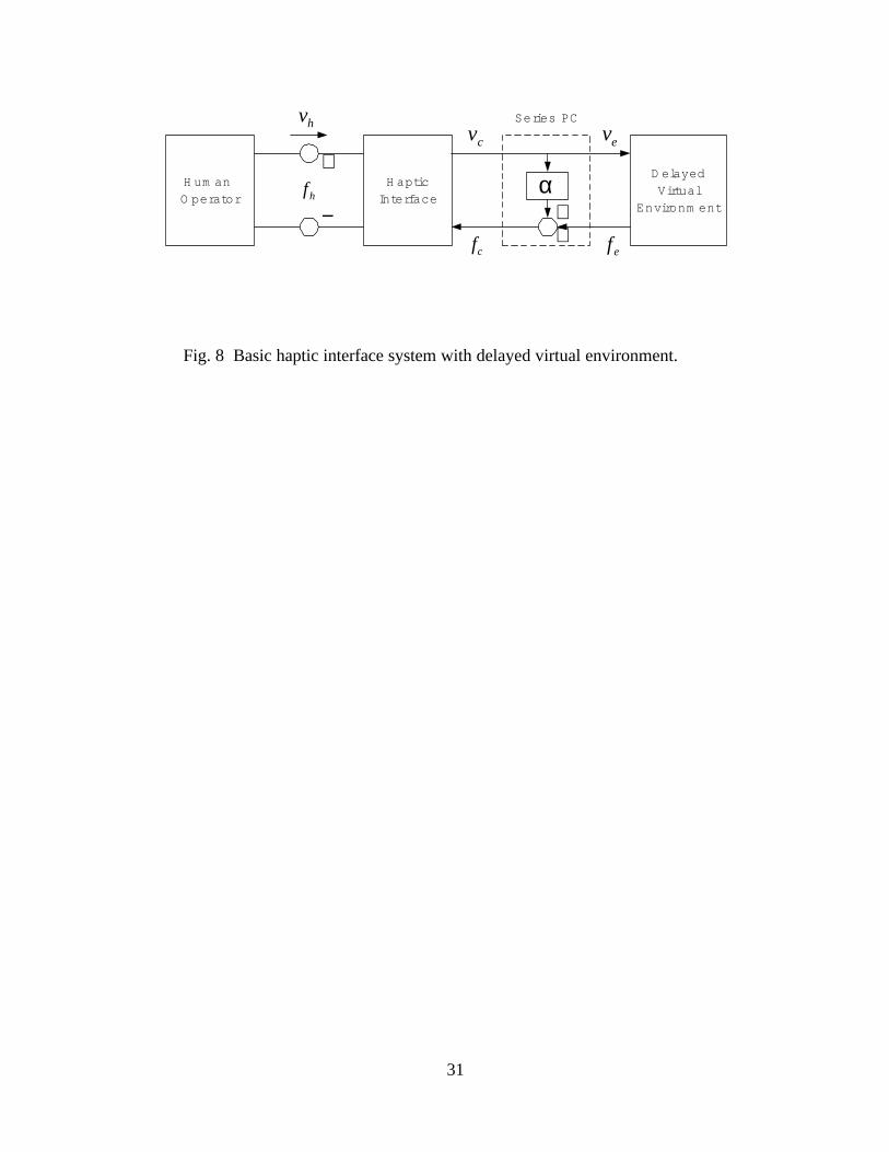
The second simulation is of a basic haptic interface system (Fig. 8) consisting of the
human operator (HO), the haptic interface (HI), the Passivity Controller (PC) and the
virtual environment (VE). Note that the series passivity controller appears in Fig. 8 to be
connected in parallel, but this is an artifact of switching to block diagram notation for the
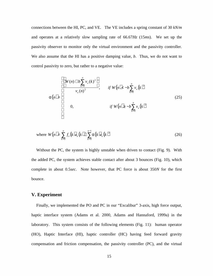
15
connections between the HI, PC, and VE. The VE includes a spring constant of 30 kN/m
and operates at a relatively slow sampling rate of 66.67Hz (15ms). We set up the
passivity observer to monitor only the virtual environment and the passivity controller.
We also assume that the HI has a positive damping value, b. Thus, we do not want to
control passivity to zero, but rather to a negative value:
( )
( ) ( )
( ) ( )
−≥
−<
+
=
∑
∑∑
=
=
=
n
ke
n
ke
e
n
ke
kvbnWif
kvbnWifnv
kvbnW
n
0
2
0
2
2
0
2
0,
,)(
)()(
α (25)
where ( ) ( ) ( ) ( ) ( )∑∑−
==
+=1
0
2
0
n
ke
n
kee kvkkvkfnW α (26)
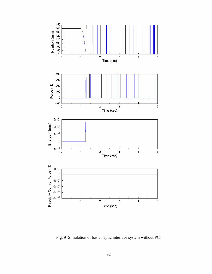
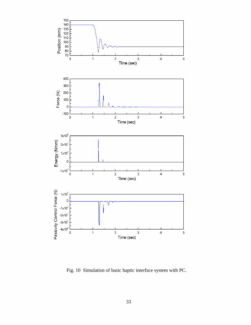
Without the PC, the system is highly unstable when driven to contact (Fig. 9). With
the added PC, the system achieves stable contact after about 3 bounces (Fig. 10), which
complete in about 0.5sec. Note however, that PC force is about 350N for the first
bounce.
V. Experiment
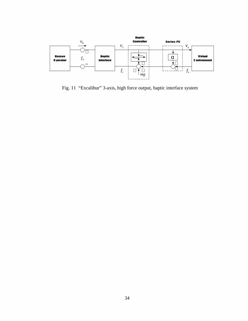
Finally, we implemented the PO and PC in our “Excalibur” 3-axis, high force output,
haptic interface system (Adams et al. 2000, Adams and Hannaford, 1999a) in the
laboratory. This system consists of the following elements (Fig. 11): human operator
(HO), Haptic Interface (HI), haptic controller (HC) having feed forward gravity
compensation and friction compensation, the passivity controller (PC), and the virtual
16
environment (VE). This system is entirely synchronous at 1000Hz. The HI senses
position in 0.1mm increments, and can display up to 200N force inside a
300x300x200mm workspace. The force resolution is 9.8gf. The virtual environment
consisted of virtual Lego-like blocks.
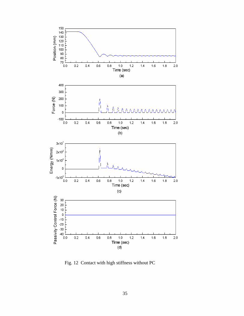
A. Contact with High Stiffness
In this experiment, the PO accounted for energy flow in the HC, PC, and VE. We also
assumed significant dissipation in the HO and HI (b = 35 Ns/m) and so used a non-zero
threshold for the PC. In the first experiment, without the PC, the operator approached the
virtual object (k = 90 kN/m) at about 200 mm/s (Fig. 12a). Contact was unstable,
resulting in an oscillation observable as force pulses (Fig. 12b), the passivity observer
(Fig. 12c) was initially positive, but grew to more and more negative values with each
contact. Interestingly, the initial bounce was passive, but the subsequent smaller bounces
were active.
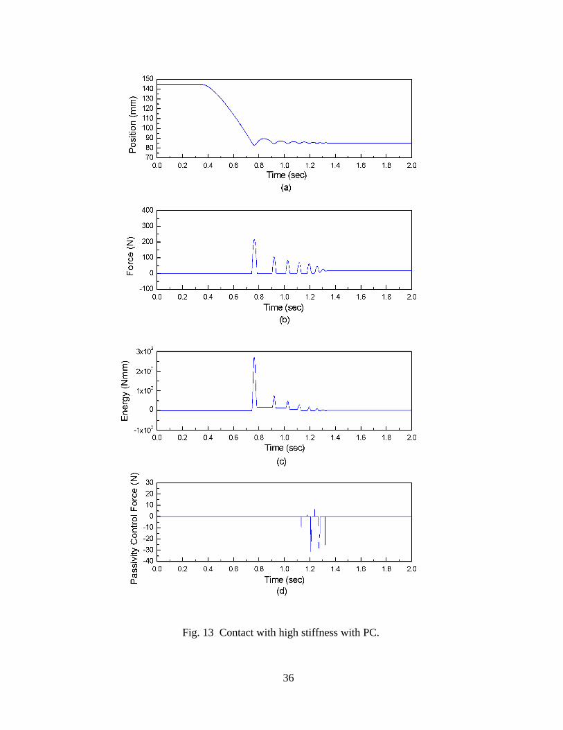
In the second experiment, with the PC turned on, the operator approached contact at
the same velocity (Fig. 13a), but stable contact was achieved with about 6 bounces (Fig.
13b). Again the first bounce can be seen to behave passively, but subsequent smaller
bounces were active (Fig. 13c). On the fourth bounce, the PC began to operate (Fig.
13d), and eliminated the oscillation. The PC force was less than 40N, well within our
actuator capabilities. However, in some cases PC force may add to other forces so we
cannot tell from this alone whether or not actuator saturation occurred.
17
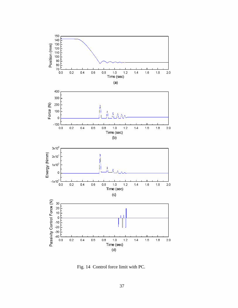
B. Control Force Limit
In the next experiment, we study the effect of limiting PC force to ±20N. The result
is almost the same (Fig. 14) with some slightly longer pulses observed in the PC output
(Fig. 14d) and some positive forces observed at the end of the PC output.
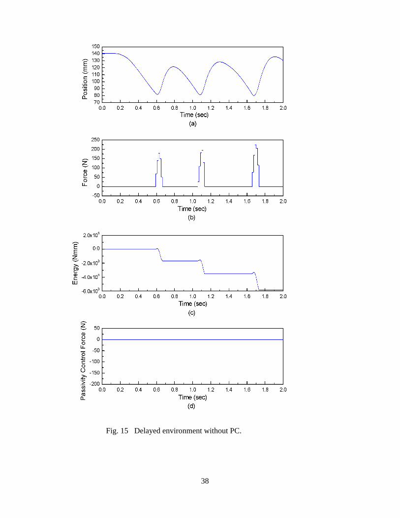
C. Delayed Environment
One of the most challenging problems for further application of haptics is application
to slow computing environments. These slow VEs are characteristic of complex
simulations such as deformable objects for surgery or macro-molecular dynamics. We
modified the basic Excalibur system to artificially slow down the VE to a rate of
66.67Hz. The output force value of the simulation was held constant for 15 samples and
then replaced with the new force value based on its input 15 samples prior. Environment
stiffness was set to 30 kN/m.
Without PC, the result is a very unstable system (Fig. 15). The sampling delay due to
the slow VE is visible in the shape of the force pulses which are as high as 200 Newtons
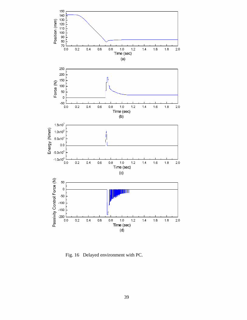
(Fig. 15b). With PC, the contact was stabilized within a single bounce (Fig. 16). The
contact force (Fig. 16b) is limited to a single pulse which tapers exponentially during
about 1 second. The PO (Fig. 16c, note change in scale) consists of a single positive peak
and is constrained to positive values. The passivity control output (Fig. 16d) consists of a
single large pulse, followed by a noise-like signal during the exponential decay of force (t
= 0.8 s to 1.2 s). The noisy behavior of the passivity controller coincides with a period of
low velocity (Fig. 16a, t = 0.8 - 1.2 s).
18
VI. Discussion
The haptic controller of the Excalibur system contains two features which are
illustrated by our analysis. First, the controller compensates for gravity by adding a force
in the positive Z direction equal to the weight of the Z-axis moving parts. This force
component is constant and independent of the applied velocity, so it could be active or
passive depending on the applied velocity. The gravity compensator will be passive over
any closed trajectory in Z.
The second component is a coulomb friction component
( ) ( )( ) 0 ,sgn >−= AkvAkFc
( )∑
∑∑
=
==
−=
−=
k
n
n
k
n
kc
kvA
kvkvAkkF
1
00
))((sgn )( )( v)(
( ) ( ) kkvkFn
kc ∀≤∑
= 0
0
(27)
Clearly the Coulomb friction compensation term is active. Applying PO’s at several
points around our Excalibur system confirmed this analysis and showed that active
behavior observed in Fig. 12 was primarily due to the friction compensation module.
The Passivity Controller has several desirable properties for applications including
haptic interface control. The passivity observer and passivity controller can both be
implemented with simple software in existing haptic interface systems. The stability can
be proven, yet it is not a fixed parameter design based on a worst case analysis. Thus, to
19
maintain stability, the PC only degrades performance (through the added damping of the
Passivity Controller) when it is needed, and only in the amount needed.
Energy storage elements in the system do not have to be modeled, only dissipation.
Dissipation in the elements outside the PO needs to be identified for optimum
performance. However, the added performance due to modeling external dissipation (i.e.,
eqn. 24) appears to be small. Thus, the PC can be very useful without any parameter
estimation at all.
Nevertheless, the method has some limitations which we considered in advance or
which become apparent in experimental testing. First, there are important cases in which
virtual environments have very different behavior in different locations. Consider an
environment which is very dissipative in location X and active in location Y. If the user
spends a lot of time interacting at X, the passivity observer may build up a large positive
value. Then, if the user moves over and interacts with location Y, the Passivity
Controller will not operate until a corresponding amount of active behavior is observed.
Theoretically, this is not a problem since even though the interaction may act unstable
initially, the amount of instability will be bounded by the accumulated dissipation.
Nevertheless, as a practical matter the amount of active behavior observed may exceed
what is desired. One possibility we are exploring is “resetting” in which we derive
heuristic rules for resetting the Passivity Observer to zero. These rules might, for
example, detect a free motion state. However, such heuristics need to be experimentally
tested in a wide variety of virtual environments.

20
Additional issues we described and tested were the performance of the system with
limits imposed on the Passivity Controller and sensitivity to low values of velocity. A
patent application is pending on this technology.
VII. Future Work
In addition to resetting, there are several areas of future work which we will pursue.
First, we identified issues associated with operation of the PC during periods of low
velocity (series) or low force (parallel). We are studying a hybrid form of PC which
includes both series and parallel dissipative elements and selects the most appropriate one
for the operating conditions.
A second issue is the identification of the dissipation constant ( β in Eq. 24) for the
human operator and haptic interface mechanism. We intend to study ways of
automatically estimating this parameter during operation.
A third issue is that of sensitivity to noise in the velocity estimate used in the
controller. This is evident in Fig. 16 when the velocity is near zero. In these conditions,
the user feels and hears some vibration for about one half second. Current work is
studying a method for eliminating this phenomenon.
Finally, the benefits of the PO/PC may apply to other types of control systems such as
motion control systems. We will study the possible applications of the PO/PC to increase
the reliability and safety of this type of system.
21
References
R. J. Adams, D. Klowden, B. Hannaford, “Stable Haptic Interaction using the ExcaliburForce Display,” Proc. IEEE Int. Conf. Robot. Automat., San Francisco, CA, 2000, pp.770-775.
R. J. Adams, B. Hannaford, “Excalibur, A Three-Axis Force Display,” ASME WinterAnnual Meeting Haptics Symposium, Nashville, TN, November, 1999a.
R. J. Adams and B. Hannaford, “Stable Haptic Interaction with Virtual Environments,”IEEE Trans. Robot. Automat., vol. 15, no. 3, pp. 465-474, 1999b.
R. J. Anderson and M. W. Spong, “Asymptotic Stability for Force ReflectingTeleoperators with Time Delay,” Int. Journal of Robotics Research, vol. 11, no. 2, pp.135-149, 1992.
L. O. Chua, C. A. Desoer, E. S. Kuh, “Linear and Nonlinear Circuits,” McGraw-Hill,New York, 1987.
J. E. Colgate, M. C. Stanley, J. M. Brown, “Issues in the Haptic Display of Tool Use,”Proc. IEEE/RSJ Int. Conf. on Intelligent Robotics and Systems, Pittsburgh, PA, 1995, pp.140-145.
J. E. Colgate, and G. Schenkel, "Passivity of a Class of Sampled-Data Systems:Application to Haptic Interfaces," american Control Conference, Baltimore, MD, 1994,pp. 3236-3240.
C. A. Desoer and M. Vidyasagar, Feedback Systems: Input-Output Properties, NewYork: Academic, 1975.
B. Gillespie and M. Cutkosky, “Stable User-Specific Rendering of the Virtual Wall,”Proc. of the ASME International Mechanical Engineering Conference and Exposition,DSC-Vol. 58, Atlanta, GA, Nov. 17-22, 1996, pp. 397-406.
B. Hannaford, “A Design Framework for Teleoperators with Kinesthetic Feedback,”IEEE Trans. Robot. Automat., vol. 5, no. 4, pp. 426-434, 1989.
N. Hogan, “Controlling Impedance at the Man/Machine,” Proc. IEEE Int. Conf. Robot.Automat., Scottsdale, AZ, 1989, pp. 1626-1631.
B. E. Miller, J. E. Colgate and R. A. Freeman, “Passive Implementation for a Class ofStatic Nonlinear Environments in Haptic Display,” Proc. IEEE Int. Conf. Robot.Automat., Detroit, Michigan, May, 1999a, pp. 2937-2942.
B. E. Miller, J. E. Colgate and R. A. Freeman, “Computational Delay and Free ModeEnvironment Design for Haptic Display,” Proc. ASME Dyn. Syst. Cont. Div., 1999b.
22
B. E. Miller, J. E. Colgate and R. A. Freeman, “Environment Delay in Haptic Systems,”Proc. IEEE Int. Conf. Robot. Automat., San Francisco, CA, April, 2000, pp. 2434-2439.
G. Niemeyer and J. J. Slotine, “Stable Adaptive Teleoperation,” IEEE Journal of OceanicEngineering, vol. 16, pp. 152-162, 1991.
H. M. Paynter, “Analysis and Design of Engineering Systems,” MIT Press, Cambridge,MA, 1961.
A.J. van der Schaft, "L2-Gain and Passivity Techniques in Nonlinear Control," Springer,Communications and Control Engineering Series, 2000.
J. C. Willems, "Dissipative Dynamical Systems, Part I: General Theory," Arch. Rat.Mech. An., vol. 45, pp. 321-351, 1972.
Y. Yokokohji, T. Imaida and T. Yoshikawa, “Bilateral Control with Energy BalanceMonitoring Under Time-Varying Communication Delay,” Proc. IEEE Int. Conf. Robot.Automat., San Francisco, CA, April, 2000, pp. 2684-2689.
C. B. Zilles and J. K. Salisbury, “A Constraint-based God-object Method for HapticDisplay,” Proc. IEEE/RSJ Int. Conf. on Intelligent Robotics and Systems, Pittsburgh, PA,1995, pp. 146-151.
Acknowledgments
We gratefully acknowledge Manuel Moreyra, Rick Adams and Dan Klowden for theExcalibur system.

23
Figure Captions
Figure 1One-port and M-port networks representing components of a haptic interface system.
Figure 2Example of arbitrarily connected network system with one open end. Each block can
be either passive or active. Entire system passivity is sum of individual blocks.
Figure 3Series (a) and parallel (b) configurations of passivity controller for one-port networks.
α is an adjustable damping element. Choice of configuration depends on input/outputcausality of model underlying the one-port.
Figure 4Series and parallel passivity controllers for two-port networks. A passivity controller
on only one of the ports is sufficient.
Figure 5Series and parallel passivity controllers for network systems.
Figure 6Simple virtual wall model for simulation testing of PO/PC.
Figure 7Simulation response for simple virtual wall system. When driven by a sinusoidal
velocity profile (a), system dissipates energy when damping is positive (b) and generatesenergy when damping is negative (c). When wall damping is still negative and passivitycontroller is operating, dissipation is constrained to be positive (d) and system is stable.
Figure 8More detailed simulation model of a complete haptic interface system and passivity
controller. System blocks are (left to right) human operator, haptic interface, passivitycontroller (α), and virtual environment.
Figure 9Simulated response of haptic interface model (Fig. 8). Passivity controller is not
operating (bottom trace) and system is unstable.
Figure 10Simulation of haptic interface system (Fig. 8) with passivity controller enabled.
Passivity controller operates briefly (bottom trace) to damp out oscillations and constrainenergy dissipation to be positive.
24
Figure 11Block diagram of experimental test system. Additional block (center) shows friction
and gravity compensation elements.
Figure 12Experimental results: contact with virtual environment (stiffness = 90 kN/m).
Passivity controller is inactive and system exhibits sustained contact oscillations.
Figure 13Experimental results: contact with same virtual environment as in Fig. 12 with
passivity controller operating. Oscillation is suppressed by brief pulses of force from PC(bottom trace). Note that initial “bounce” behaved passively, but subsequent smallerbounces were active.
Figure 14Experimental results: same conditions as Fig. 12, but passivity controller force
limited to ±20 N. System is stable despite imposing a force limit to represent actuatorsaturation.
Figure 15Experimental results: stiffness reduced to 30 kN/m, but virtual environment slowed
down to 67Hz instead of 1000 Hz. Passivity controller is off and the system is highlyunstable.
Figure 16Experimental results: same conditions as Fig. 15, but passivity controller is enabled.
System now achieves stable, steady state, contact.
25
N
v
f+
−
MN
1v
1f
kv
kf
M
1+kv
1+kf
Mv
Mf
M
+−
+−
+−
3N
1v
1f 1N
3v
3f
2N
4N
MN
5v
5f
Mv
Mf
2v2f
4v 4f
+
−
+
−
+ −
+ −
+
−
+
−
(a) One-port network (b) M-port network
Fig. 1 One-port and M-port networks
Fig. 2 Example of arbitrarily connected network system with one open-end.
26
Nα
2v
2f
P.C
+
−
+
−
1v
1f
N
2v
2f
P.C
+
−
+
−
1v
α1f
(a) Series or velocity conserving Passivity Controller.
(b) Parallel or force conserving Passivity Controller.
Fig. 3 Configuration of Passivity Controller for one-port networks
27
LNα
2v
1f
P.C
+
−
+
−
1v 3v
2f+
−3f
LN
2v
2f
P.C
+
−
+
−
1v 3v
3f+
−α
1f
(a) Series or velocity conserving.
(b) Parallel or force conserving
Fig. 4 Configuration of Passivity Controller for two-port networks
28
(a) Series or velocity conserving
(b) Parallel or force conserving
Fig. 5 Configuration of Passivity Controller for network systems
2N
3v
3f+
−LNα
2v
1f
P.C
+
−
+
−
1v
2f
2N
3v
3f+
−LN
2v
2f
P.C
+
−
+
−
1v
α1f
29
Fig. 6 Impedance type virtual wall
( )tf
( )tv
k
b
α
30
Fig. 7 Energy behavior of impedance type virtual wall.
31
Fig. 8 Basic haptic interface system with delayed virtual environment.
H um an O perator
H apticInterface
D elayedVirtual
Environm ent
α+
++−
hf
hv
cf
cv
ef
evSeries PC
32
Fig. 9 Simulation of basic haptic interface system without PC.
33
Fig. 10 Simulation of basic haptic interface system with PC.
34
Fig. 11 “Excalibur” 3-axis, high force output, haptic interface system
Human
O perator
Haptic
Interface
+
−hf
hv
cf
cvSeries PC
V irtual
E nvironmentα
++
ef
ev
+++
mg
Haptic
Controller
35
Fig. 12 Contact with high stiffness without PC
36
Fig. 13 Contact with high stiffness with PC.
37
Fig. 14 Control force limit with PC.
38
Fig. 15 Delayed environment without PC.
39
Fig. 16 Delayed environment with PC.