Embed Size (px)
Citation preview
Time-Frequency Analysis
PhD Course November 10, 11,and December 1, 2, 2003.
Arne Jensen
Aalborg University
Time-Frequency Analysis – p.1/96
Overview
The purpose of this course is to give you an introduction totime-frequency analysis. Many of you have already hadsome exposure to this topic, so a secondary purpose is totry to answer some of your questions concerningtime-frequency analysis. It is a highly nontrivial subject,both from the theoretical side, and from the applied side.
Prerequisites: Some knowledge of Fourier Analysis andSignal Processing.
Query: Your background?
Time-Frequency Analysis – p.2/96
Course description
Description: The purpose of this course is to introduce theparticipants to time-frequency analysis. A jointtime-frequency analysis of a signal can often reveal thefeatures in complicated signals. It is difficult to perform ajoint time-frequency analysis, due to the fundamentallimitations imposed by the uncertainty principle.Compromises between resolution in time and in frequencymust always be made. The course will give an introductionto this area. Topics include:
Time-Frequency Analysis – p.3/96
Course description
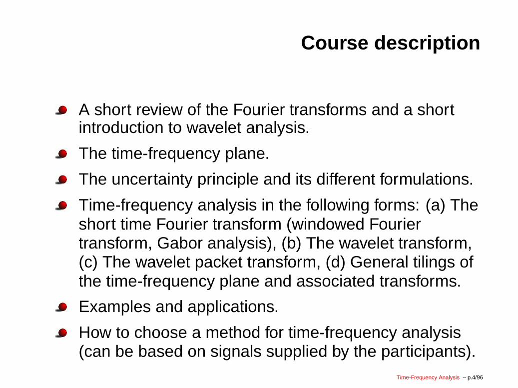
A short review of the Fourier transforms and a shortintroduction to wavelet analysis.
The time-frequency plane.
The uncertainty principle and its different formulations.
Time-frequency analysis in the following forms: (a) Theshort time Fourier transform (windowed Fouriertransform, Gabor analysis), (b) The wavelet transform,(c) The wavelet packet transform, (d) General tilings ofthe time-frequency plane and associated transforms.
Examples and applications.
How to choose a method for time-frequency analysis(can be based on signals supplied by the participants).
Time-Frequency Analysis – p.4/96
Course description
A short review of the Fourier transforms and a shortintroduction to wavelet analysis.
The time-frequency plane.
The uncertainty principle and its different formulations.
Time-frequency analysis in the following forms: (a) Theshort time Fourier transform (windowed Fouriertransform, Gabor analysis), (b) The wavelet transform,(c) The wavelet packet transform, (d) General tilings ofthe time-frequency plane and associated transforms.
Examples and applications.
How to choose a method for time-frequency analysis(can be based on signals supplied by the participants).
Time-Frequency Analysis – p.4/96
References
I will use following the book for the material on the discretewavelet transform, the wavelet packet transform, and theintroduction to the time-frequency plane.
A. Jensen and A. la Cour-Harbo:Ripples in MathematicsThe Discrete Wavelet TransformSpringer-Verlag 2001.
You will need to refer to your books on signal procesing orother subjects for introductory Fourier Analysis.A general introduction to the theory behind time-frequencyanalysis is
K. Gröchenig: Foundations of Time-Frequency AnalysisBirkhäuser 2000.
Time-Frequency Analysis – p.5/96

Monday November 10
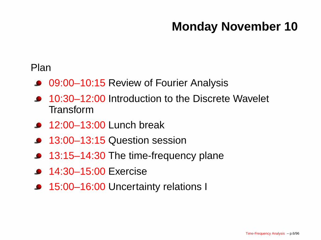
Plan
09:00–10:15 Review of Fourier Analysis
10:30–12:00 Introduction to the Discrete WaveletTransform
12:00–13:00 Lunch break
13:00–13:15 Question session
13:15–14:30 The time-frequency plane
14:30–15:00 Exercise
15:00–16:00 Uncertainty relations I
Time-Frequency Analysis – p.6/96
Monday November 10
Plan
09:00–10:15 Review of Fourier Analysis
10:30–12:00 Introduction to the Discrete WaveletTransform
12:00–13:00 Lunch break
13:00–13:15 Question session
13:15–14:30 The time-frequency plane
14:30–15:00 Exercise
15:00–16:00 Uncertainty relations I
Time-Frequency Analysis – p.6/96

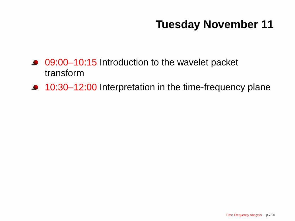
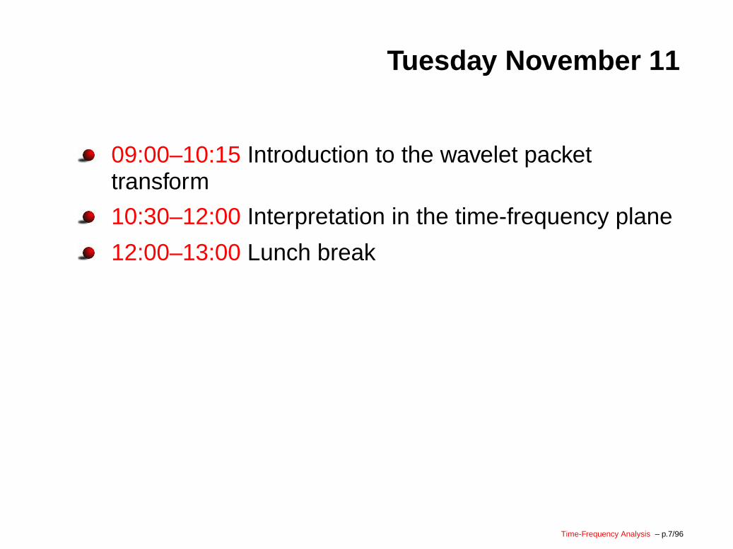
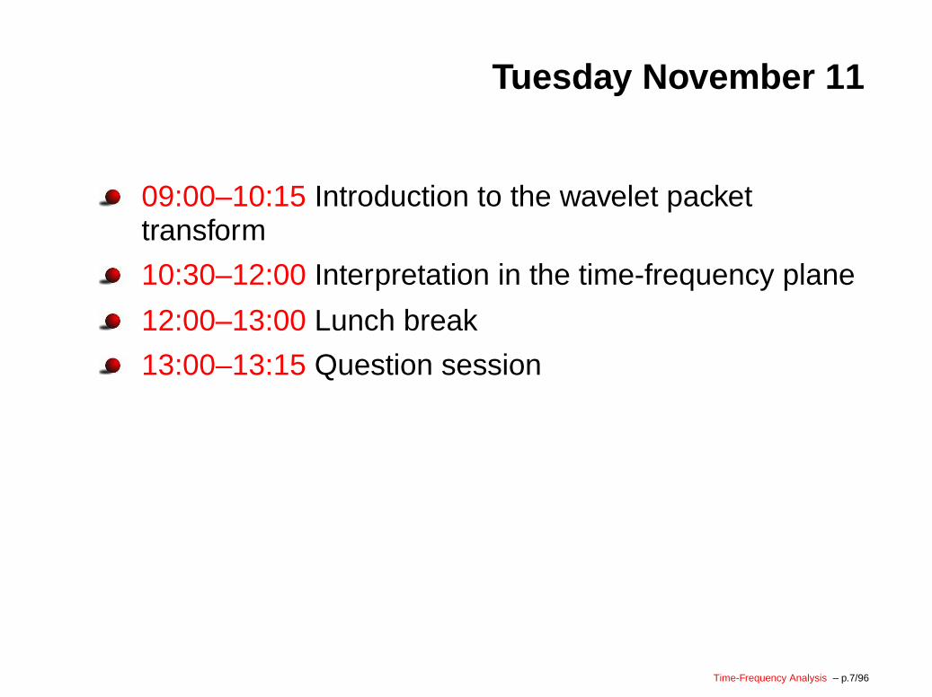
Tuesday November 11
09:00–10:15 Introduction to the wavelet packettransform
10:30–12:00 Interpretation in the time-frequency plane
12:00–13:00 Lunch break
13:00–13:15 Question session
13:15–14:30 More Fourier analysis: Gabor transforms
14:30–15:00 Exercise
15:00–16:00 Problems sets
Time-Frequency Analysis – p.7/96
Part 1
Review of Fourier Analysis
Time-Frequency Analysis – p.8/96
The Fourier transform
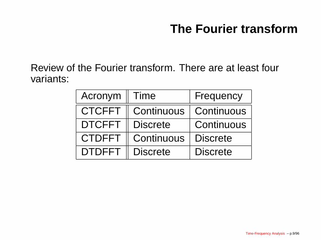
Review of the Fourier transform. There are at least fourvariants:
Acronym Time Frequency
CTCFFT Continuous ContinuousDTCFFT Discrete ContinuousCTDFFT Continuous DiscreteDTDFFT Discrete Discrete
Time-Frequency Analysis – p.9/96
The Fourier transform
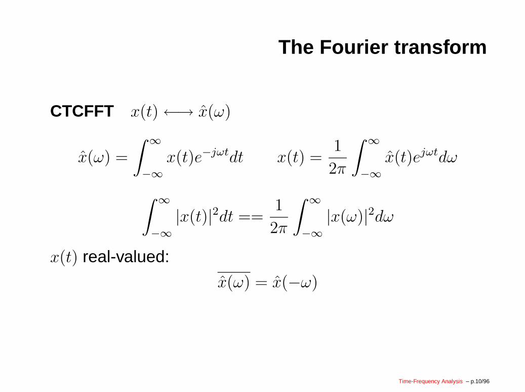
CTCFFT x(t)←→ x̂(ω)
x̂(ω) =
∫∞
−∞
x(t)e−jωtdt x(t) =1
2π
∫∞
−∞
x̂(t)ejωtdω
∫∞
−∞
|x(t)|2dt ==1
2π
∫∞
−∞
|x(ω)|2dω
x(t) real-valued:
x̂(ω) = x̂(−ω)
Time-Frequency Analysis – p.10/96
The Fourier transform
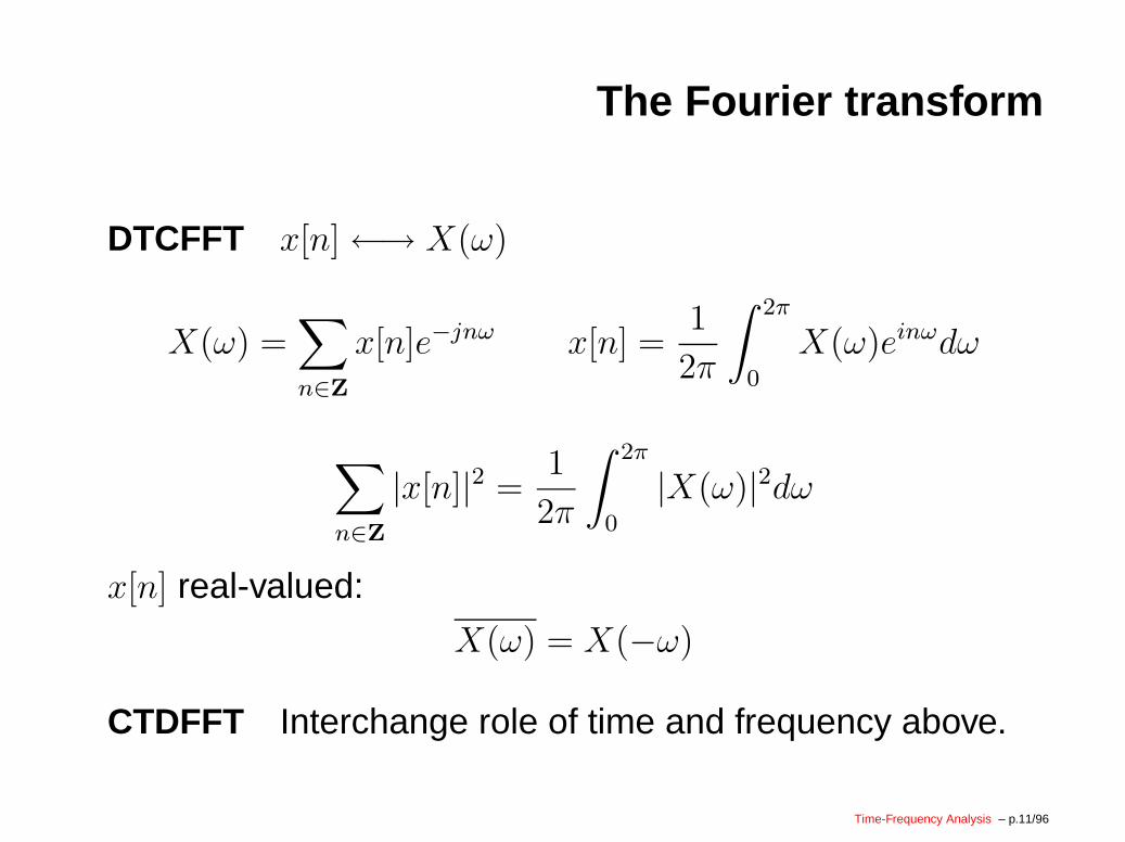
DTCFFT x[n]←→ X(ω)
X(ω) =∑
n∈Z
x[n]e−jnω x[n] =1
2π
∫ 2π
0
X(ω)einωdω
∑
n∈Z
|x[n]|2 =1
2π
∫ 2π
0
|X(ω)|2dω
x[n] real-valued:
X(ω) = X(−ω)
CTDFFT Interchange role of time and frequency above.
Time-Frequency Analysis – p.11/96
The Fourier transform
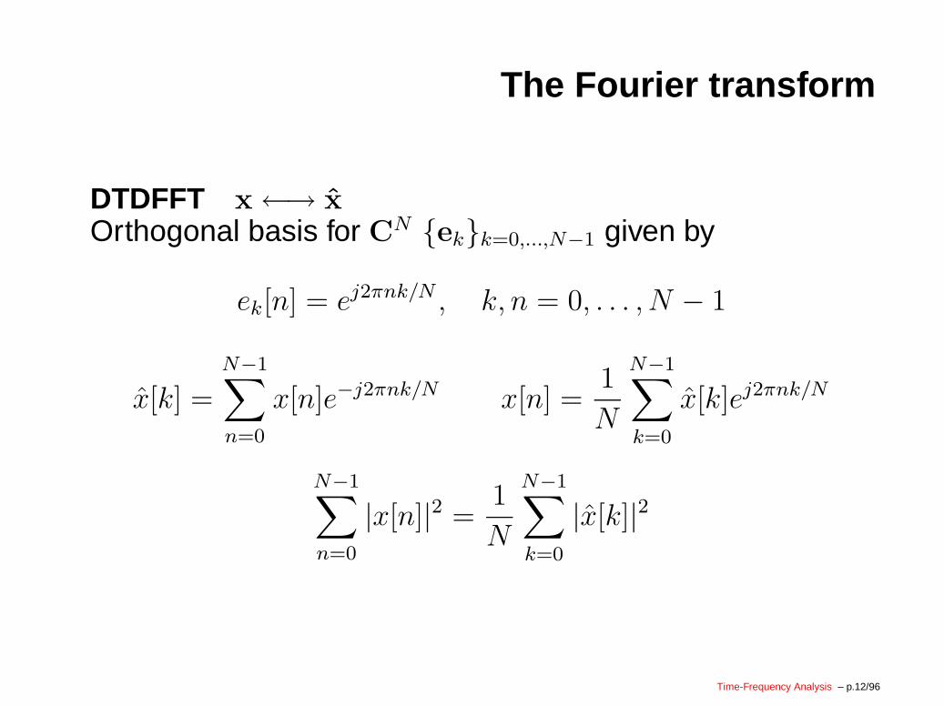
DTDFFT x←→ x̂
Orthogonal basis for CN {ek}k=0,...,N−1 given by
ek[n] = ej2πnk/N , k, n = 0, . . . , N − 1
x̂[k] =
N−1∑
n=0
x[n]e−j2πnk/N x[n] =1
N
N−1∑
k=0
x̂[k]ej2πnk/N
N−1∑
n=0
|x[n]|2 =1
N
N−1∑
k=0
|x̂[k]|2
Time-Frequency Analysis – p.12/96
The Fourier transform
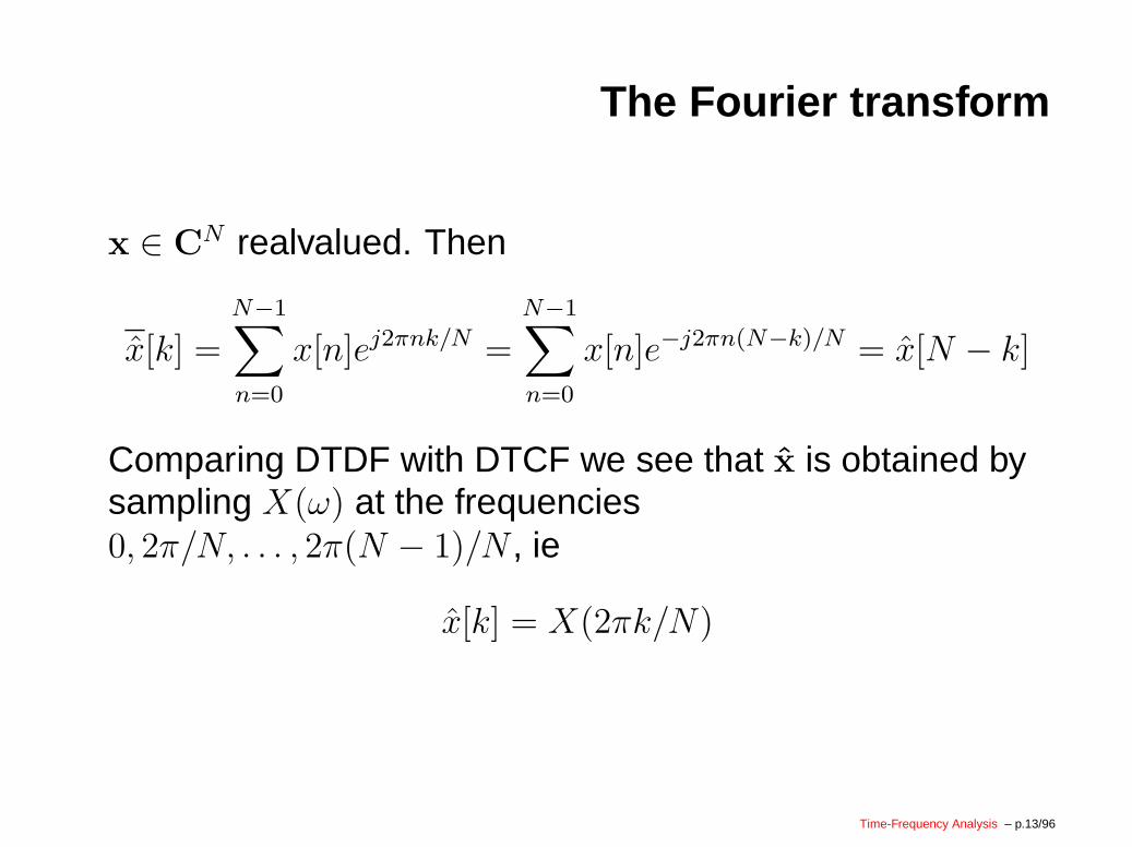
x ∈ CN realvalued. Then
x̂[k] =
N−1∑
n=0
x[n]ej2πnk/N =
N−1∑
n=0
x[n]e−j2πn(N−k)/N = x̂[N − k]
Comparing DTDF with DTCF we see that x̂ is obtained bysampling X(ω) at the frequencies0, 2π/N, . . . , 2π(N − 1)/N , ie
x̂[k] = X(2πk/N)
Time-Frequency Analysis – p.13/96
Sampling
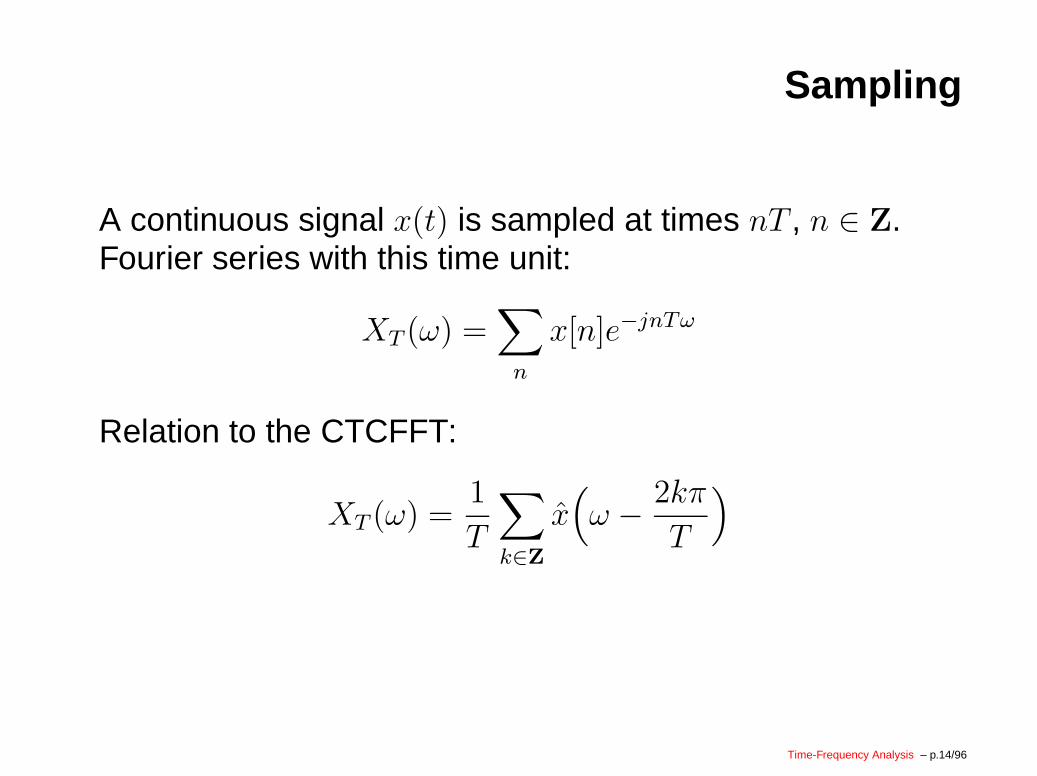
A continuous signal x(t) is sampled at times nT , n ∈ Z.Fourier series with this time unit:
XT (ω) =∑
n
x[n]e−jnTω
Relation to the CTCFFT:
XT (ω) =1
T
∑
k∈Z
x̂(
ω − 2kπ
T
)
Time-Frequency Analysis – p.14/96
Sampling
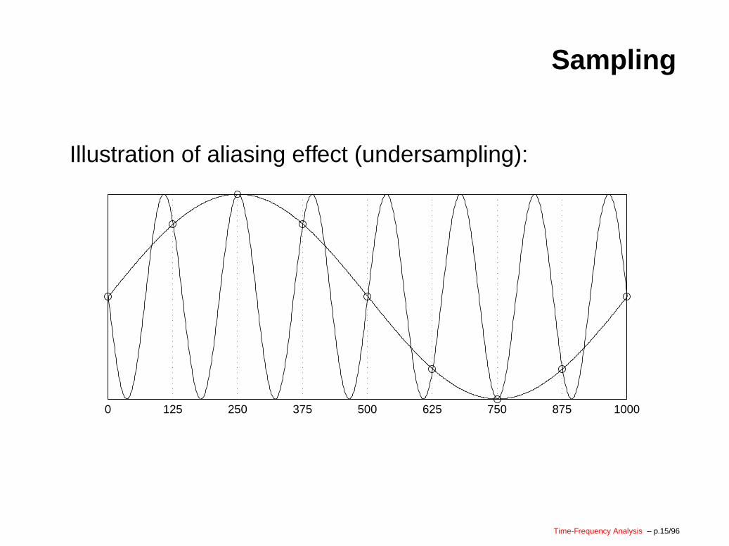
Illustration of aliasing effect (undersampling):
0 125 250 375 500 625 750 875 1000
Time-Frequency Analysis – p.15/96
Short Time Fourier Transform
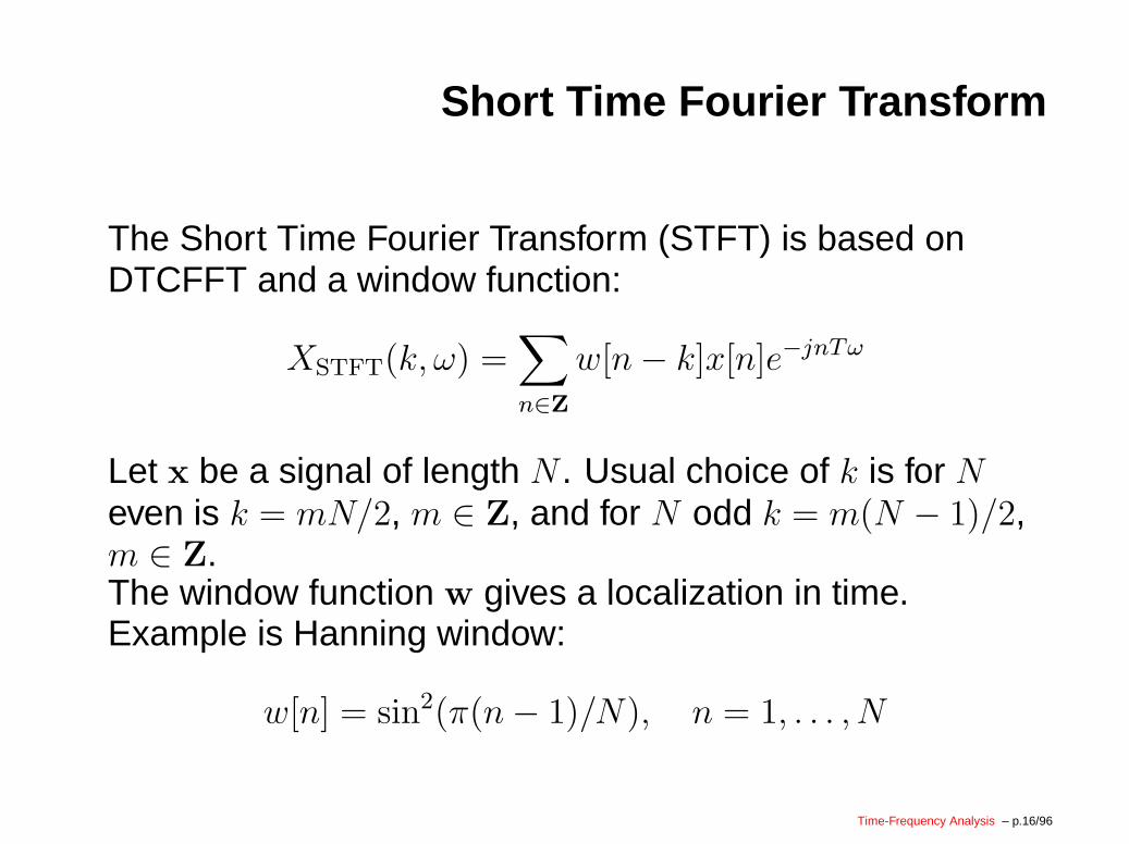
The Short Time Fourier Transform (STFT) is based onDTCFFT and a window function:
XSTFT(k, ω) =∑
n∈Z
w[n− k]x[n]e−jnTω
Let x be a signal of length N . Usual choice of k is for Neven is k = mN/2, m ∈ Z, and for N odd k = m(N − 1)/2,m ∈ Z.The window function w gives a localization in time.Example is Hanning window:
w[n] = sin2(π(n− 1)/N), n = 1, . . . , N
Time-Frequency Analysis – p.16/96
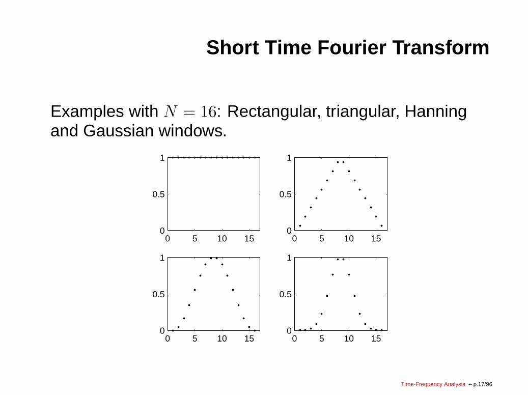
Short Time Fourier Transform
Examples with N = 16: Rectangular, triangular, Hanningand Gaussian windows.
0 5 10 150
0.5
1
0 5 10 150
0.5
1
0 5 10 150
0.5
1
0 5 10 150
0.5
1
Time-Frequency Analysis – p.17/96
Short Time Fourier Transform
The spectrogram is obtained by plotting
1
2π|XSTFT(k, 2πn/N)|2
for values of k determined by the length of the window, andfor n = 0, . . . , N − 1. Visualized in the time-frequency planeby using cells of a size determined by the length of thewindow in the frequency direction and by the length of thesignal and the overlap in the time direction.Examples will be shown later.
Time-Frequency Analysis – p.18/96
Part 2
Introduction to the Discrete Wavelet
Transform
Time-Frequency Analysis – p.19/96
A first example 1
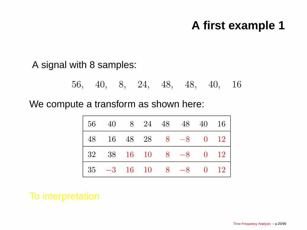
A signal with 8 samples:
56, 40, 8, 24, 48, 48, 40, 16
We compute a transform as shown here:
56 40 8 24 48 48 40 16
48 16 48 28 8 −8 0 12
32 38 16 10 8 −8 0 12
35 −3 16 10 8 −8 0 12
To interpretation
Time-Frequency Analysis – p.20/96
A first example 2
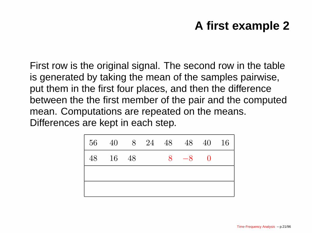
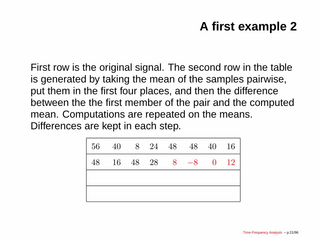
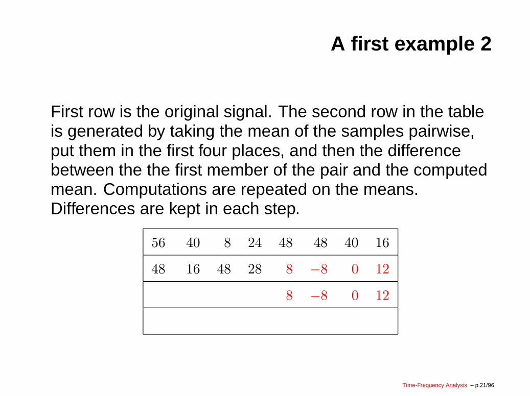
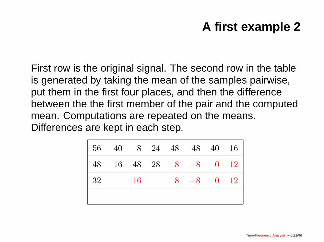
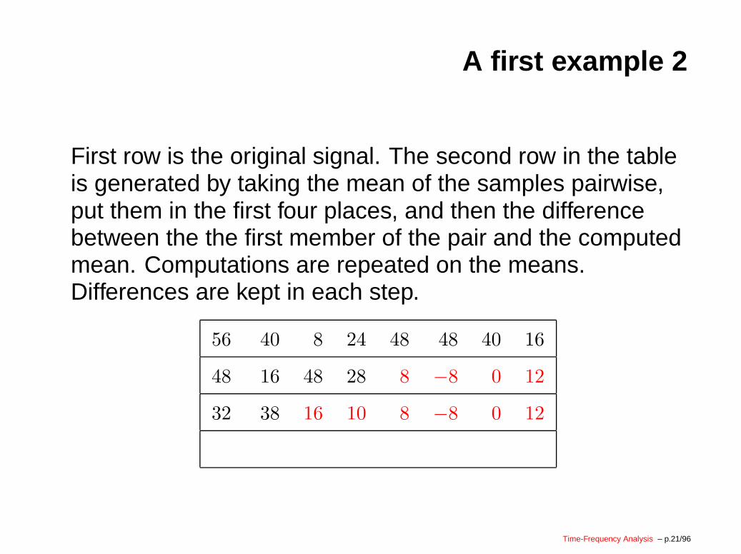
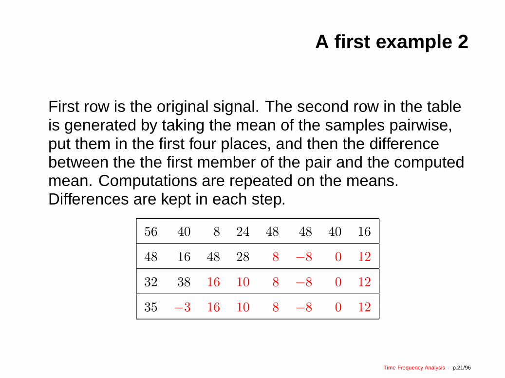
First row is the original signal. The second row in the tableis generated by taking the mean of the samples pairwise,put them in the first four places, and then the differencebetween the the first member of the pair and the computedmean. Computations are repeated on the means.Differences are kept in each step.
Time-Frequency Analysis – p.21/96
A first example 2
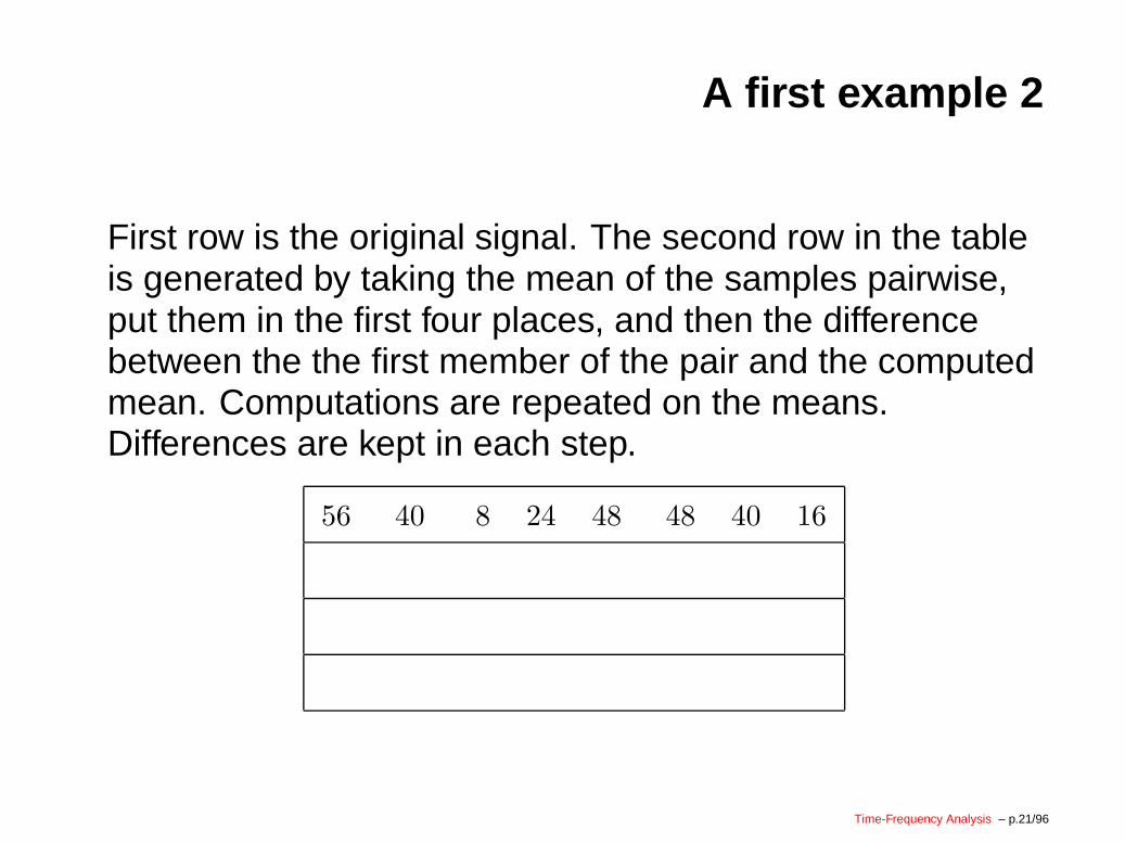
First row is the original signal. The second row in the tableis generated by taking the mean of the samples pairwise,put them in the first four places, and then the differencebetween the the first member of the pair and the computedmean. Computations are repeated on the means.Differences are kept in each step.
56 40 8 24 48 48 40 16
Time-Frequency Analysis – p.21/96
A first example 2
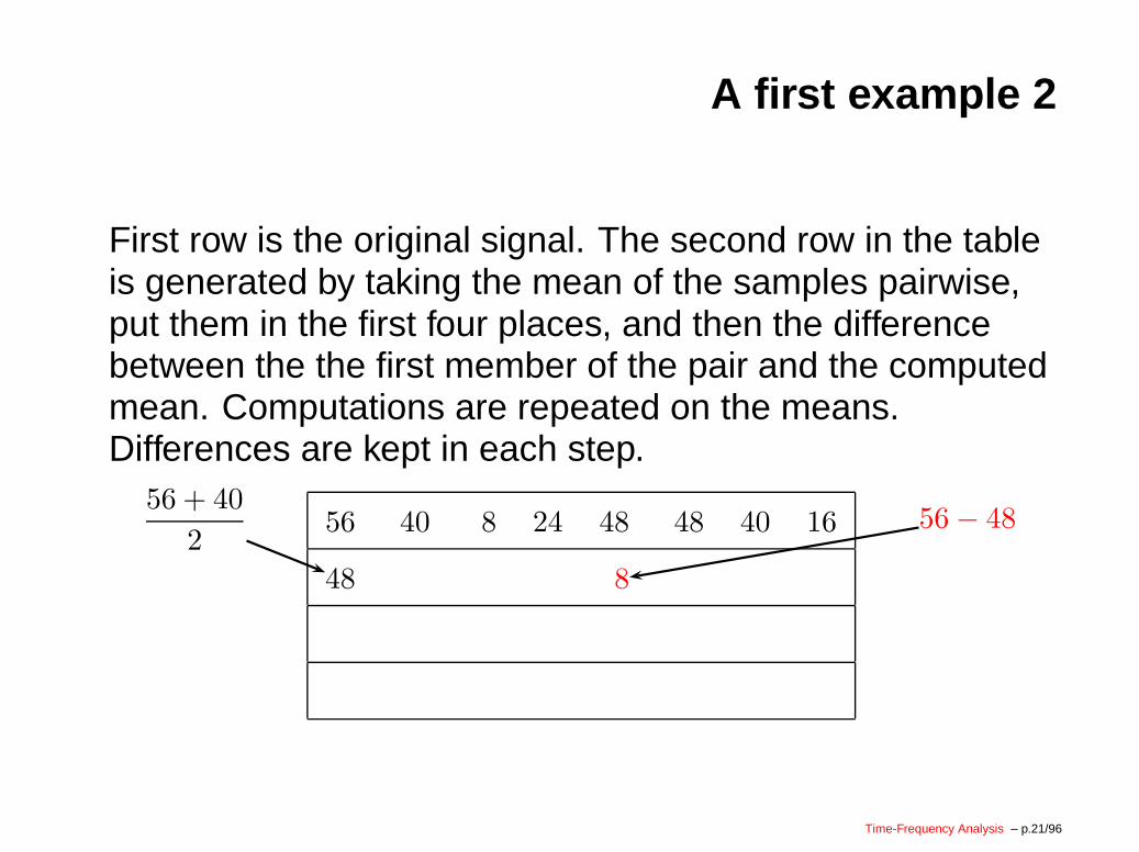
First row is the original signal. The second row in the tableis generated by taking the mean of the samples pairwise,put them in the first four places, and then the differencebetween the the first member of the pair and the computedmean. Computations are repeated on the means.Differences are kept in each step.
56 40 8 24 48 48 40 16
48 8
56 + 40
256− 48
Time-Frequency Analysis – p.21/96
A first example 2
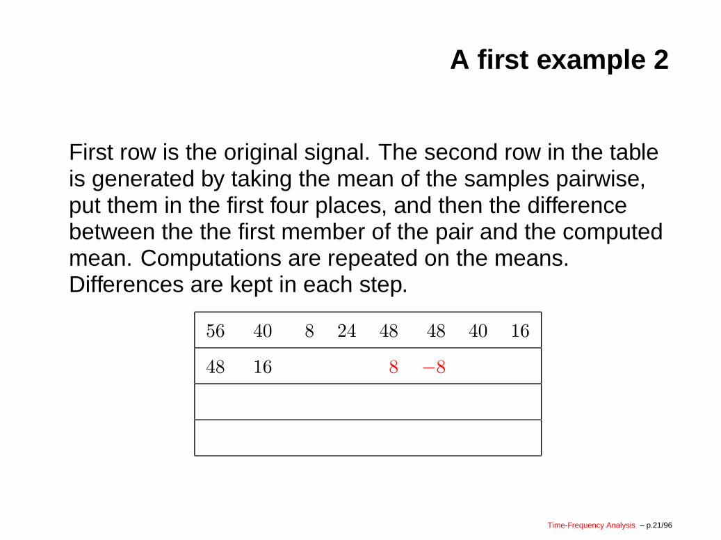
First row is the original signal. The second row in the tableis generated by taking the mean of the samples pairwise,put them in the first four places, and then the differencebetween the the first member of the pair and the computedmean. Computations are repeated on the means.Differences are kept in each step.
56 40 8 24 48 48 40 16
48 16 8 −8
Time-Frequency Analysis – p.21/96
A first example 2
First row is the original signal. The second row in the tableis generated by taking the mean of the samples pairwise,put them in the first four places, and then the differencebetween the the first member of the pair and the computedmean. Computations are repeated on the means.Differences are kept in each step.
56 40 8 24 48 48 40 16
48 16 48 8 −8 0
Time-Frequency Analysis – p.21/96
A first example 2
First row is the original signal. The second row in the tableis generated by taking the mean of the samples pairwise,put them in the first four places, and then the differencebetween the the first member of the pair and the computedmean. Computations are repeated on the means.Differences are kept in each step.
56 40 8 24 48 48 40 16
48 16 48 28 8 −8 0 12
8 −8 0 12
Time-Frequency Analysis – p.21/96
A first example 2
First row is the original signal. The second row in the tableis generated by taking the mean of the samples pairwise,put them in the first four places, and then the differencebetween the the first member of the pair and the computedmean. Computations are repeated on the means.Differences are kept in each step.
56 40 8 24 48 48 40 16
48 16 48 28 8 −8 0 12
32 16 8 −8 0 12
Time-Frequency Analysis – p.21/96
A first example 2
First row is the original signal. The second row in the tableis generated by taking the mean of the samples pairwise,put them in the first four places, and then the differencebetween the the first member of the pair and the computedmean. Computations are repeated on the means.Differences are kept in each step.
56 40 8 24 48 48 40 16
48 16 48 28 8 −8 0 12
32 38 16 10 8 −8 0 12
Time-Frequency Analysis – p.21/96

A first example 2
First row is the original signal. The second row in the tableis generated by taking the mean of the samples pairwise,put them in the first four places, and then the differencebetween the the first member of the pair and the computedmean. Computations are repeated on the means.Differences are kept in each step.
56 40 8 24 48 48 40 16
48 16 48 28 8 −8 0 12
32 38 16 10 8 −8 0 12
16 10 8 −8 0 12
Time-Frequency Analysis – p.21/96
A first example 2
First row is the original signal. The second row in the tableis generated by taking the mean of the samples pairwise,put them in the first four places, and then the differencebetween the the first member of the pair and the computedmean. Computations are repeated on the means.Differences are kept in each step.
56 40 8 24 48 48 40 16
48 16 48 28 8 −8 0 12
32 38 16 10 8 −8 0 12
35 −3 16 10 8 −8 0 12
Time-Frequency Analysis – p.21/96
A first example 3
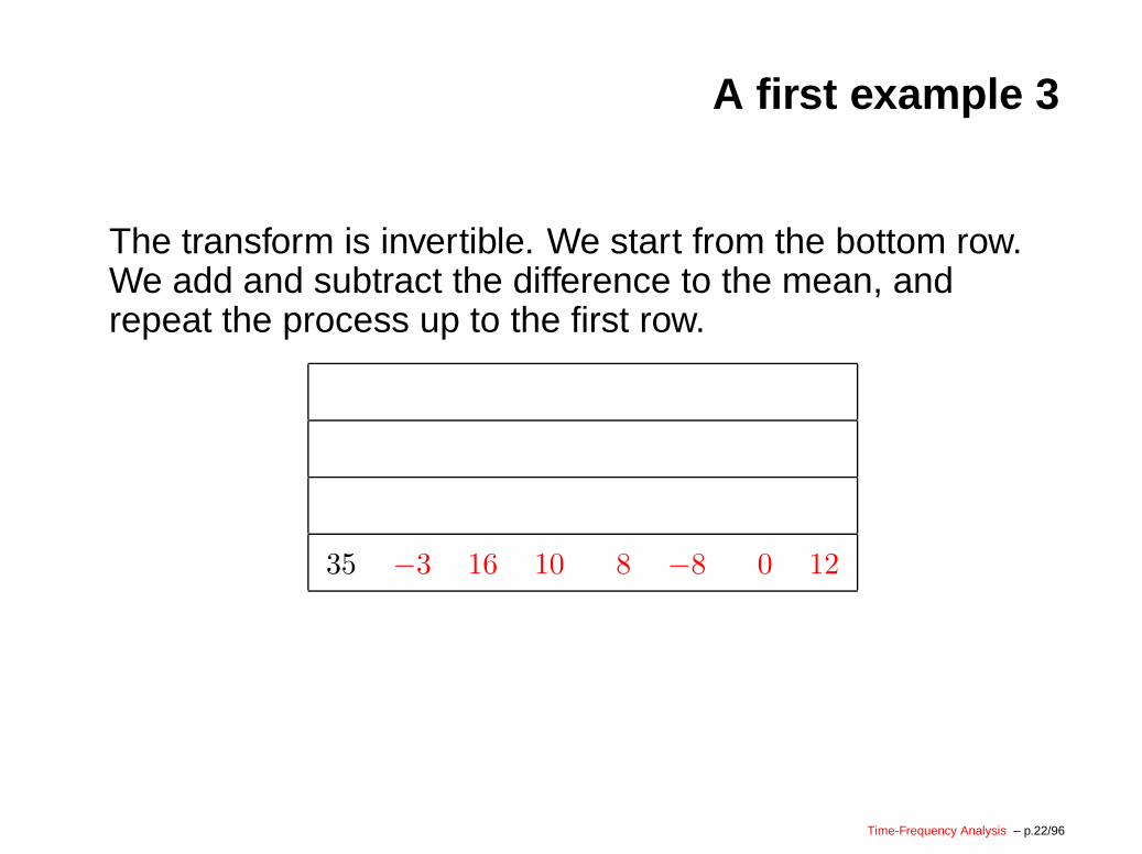
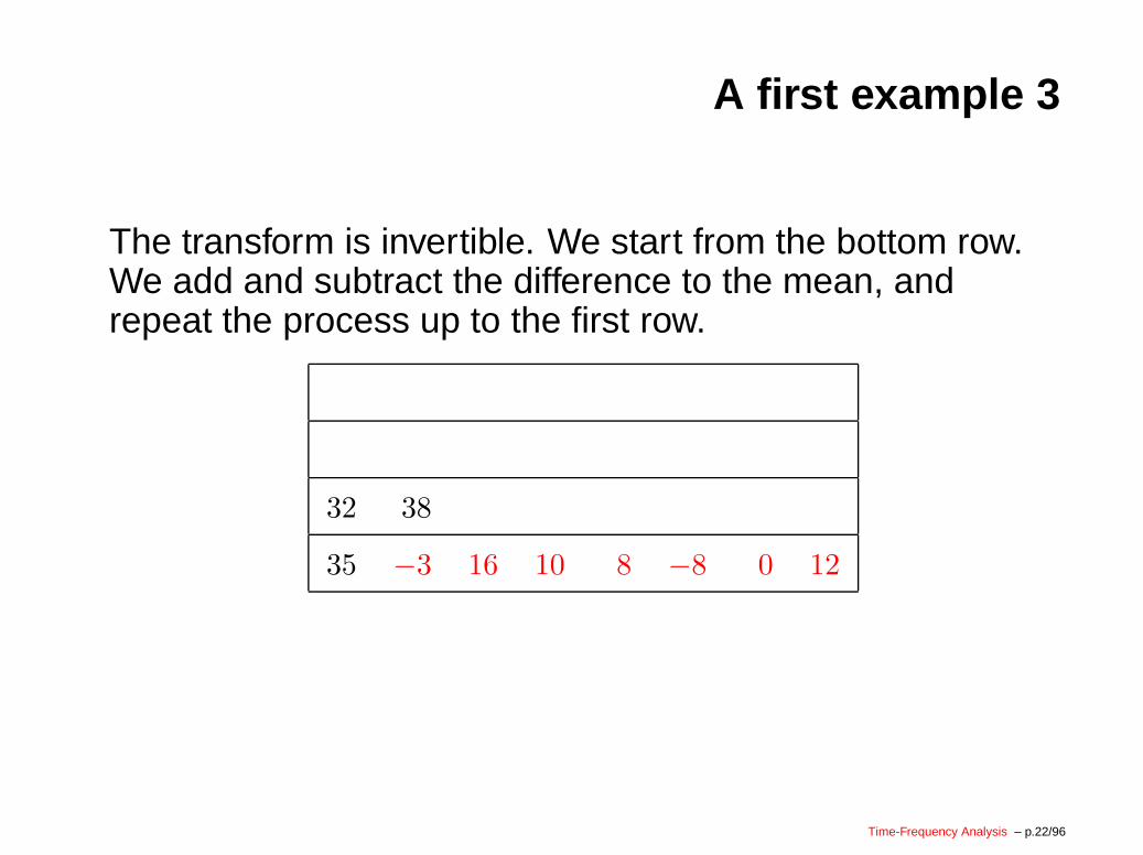
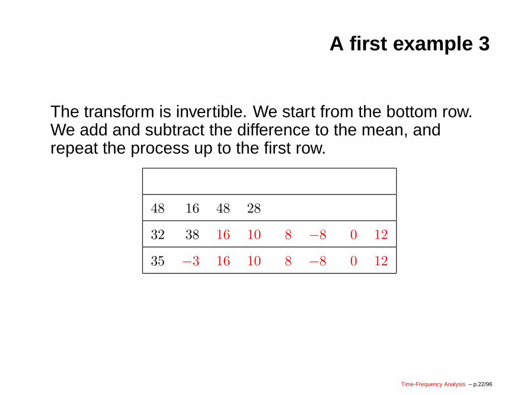
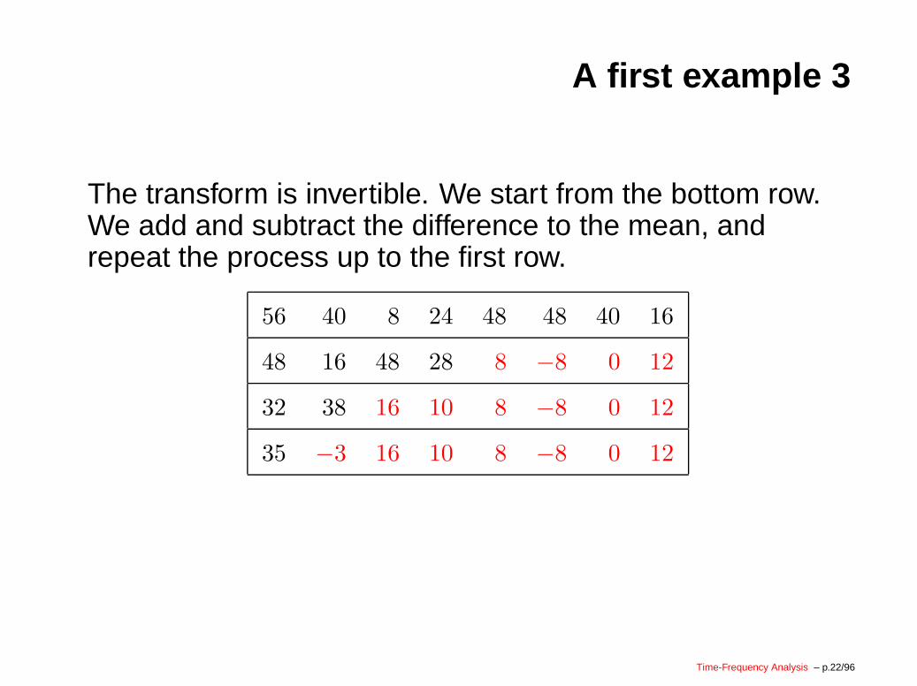
The transform is invertible. We start from the bottom row.We add and subtract the difference to the mean, andrepeat the process up to the first row.
Time-Frequency Analysis – p.22/96
A first example 3
The transform is invertible. We start from the bottom row.We add and subtract the difference to the mean, andrepeat the process up to the first row.
35 −3 16 10 8 −8 0 12
Time-Frequency Analysis – p.22/96
A first example 3
The transform is invertible. We start from the bottom row.We add and subtract the difference to the mean, andrepeat the process up to the first row.
32 38
35 −3 16 10 8 −8 0 12
Time-Frequency Analysis – p.22/96

A first example 3
The transform is invertible. We start from the bottom row.We add and subtract the difference to the mean, andrepeat the process up to the first row.
32 38 16 10 8 −8 0 12
35 −3 16 10 8 −8 0 12
Time-Frequency Analysis – p.22/96
A first example 3
The transform is invertible. We start from the bottom row.We add and subtract the difference to the mean, andrepeat the process up to the first row.
48 16 48 28
32 38 16 10 8 −8 0 12
35 −3 16 10 8 −8 0 12
Time-Frequency Analysis – p.22/96

A first example 3
The transform is invertible. We start from the bottom row.We add and subtract the difference to the mean, andrepeat the process up to the first row.
48 16 48 28 8 −8 0 12
32 38 16 10 8 −8 0 12
35 −3 16 10 8 −8 0 12
Time-Frequency Analysis – p.22/96
A first example 3
The transform is invertible. We start from the bottom row.We add and subtract the difference to the mean, andrepeat the process up to the first row.
56 40 8 24 48 48 40 16
48 16 48 28 8 −8 0 12
32 38 16 10 8 −8 0 12
35 −3 16 10 8 −8 0 12
Time-Frequency Analysis – p.22/96
A first example 4
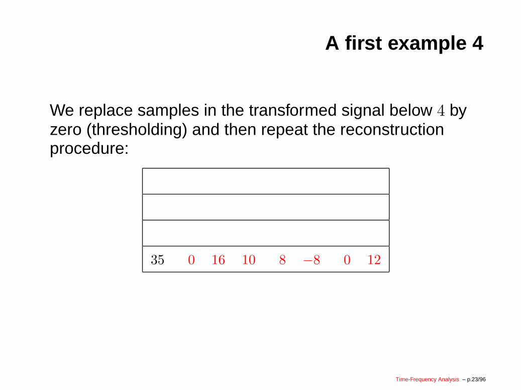
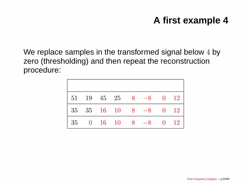
We replace samples in the transformed signal below 4 byzero (thresholding) and then repeat the reconstructionprocedure:
Time-Frequency Analysis – p.23/96
A first example 4
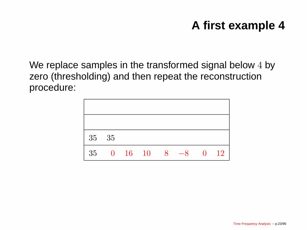
We replace samples in the transformed signal below 4 byzero (thresholding) and then repeat the reconstructionprocedure:
35 0 16 10 8 −8 0 12
Time-Frequency Analysis – p.23/96
A first example 4
We replace samples in the transformed signal below 4 byzero (thresholding) and then repeat the reconstructionprocedure:
35 35
35 0 16 10 8 −8 0 12
Time-Frequency Analysis – p.23/96
A first example 4
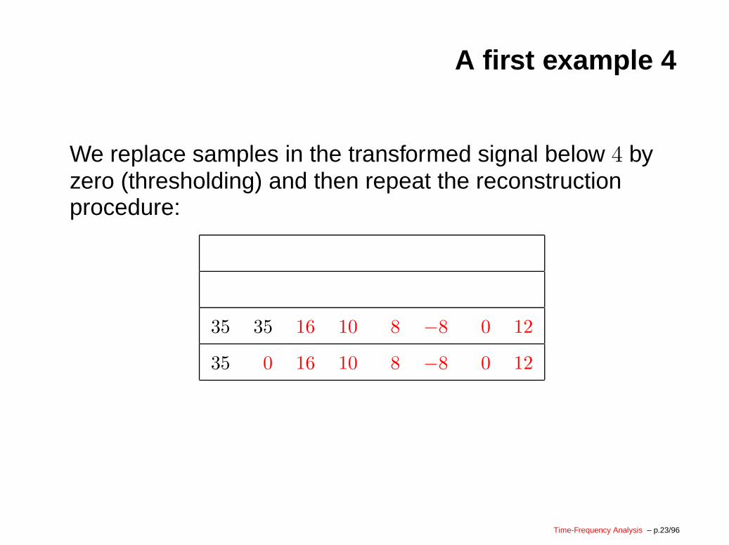
We replace samples in the transformed signal below 4 byzero (thresholding) and then repeat the reconstructionprocedure:
35 35 16 10 8 −8 0 12
35 0 16 10 8 −8 0 12
Time-Frequency Analysis – p.23/96
A first example 4
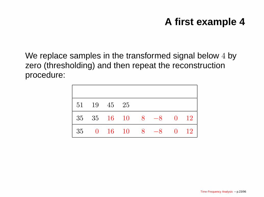
We replace samples in the transformed signal below 4 byzero (thresholding) and then repeat the reconstructionprocedure:
51 19 45 25
35 35 16 10 8 −8 0 12
35 0 16 10 8 −8 0 12
Time-Frequency Analysis – p.23/96
A first example 4
We replace samples in the transformed signal below 4 byzero (thresholding) and then repeat the reconstructionprocedure:
51 19 45 25 8 −8 0 12
35 35 16 10 8 −8 0 12
35 0 16 10 8 −8 0 12
Time-Frequency Analysis – p.23/96

A first example 4
We replace samples in the transformed signal below 4 byzero (thresholding) and then repeat the reconstructionprocedure:
59 43 11 27 45 45 37 13
51 19 45 25 8 −8 0 12
35 35 16 10 8 −8 0 12
35 0 16 10 8 −8 0 12
Time-Frequency Analysis – p.23/96
A first example 5
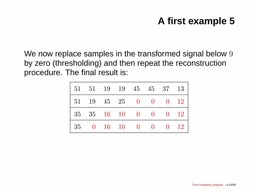
We now replace samples in the transformed signal below 9by zero (thresholding) and then repeat the reconstructionprocedure. The final result is:
51 51 19 19 45 45 37 13
51 19 45 25 0 0 0 12
35 35 16 10 0 0 0 12
35 0 16 10 0 0 0 12
Time-Frequency Analysis – p.24/96
A first example 6
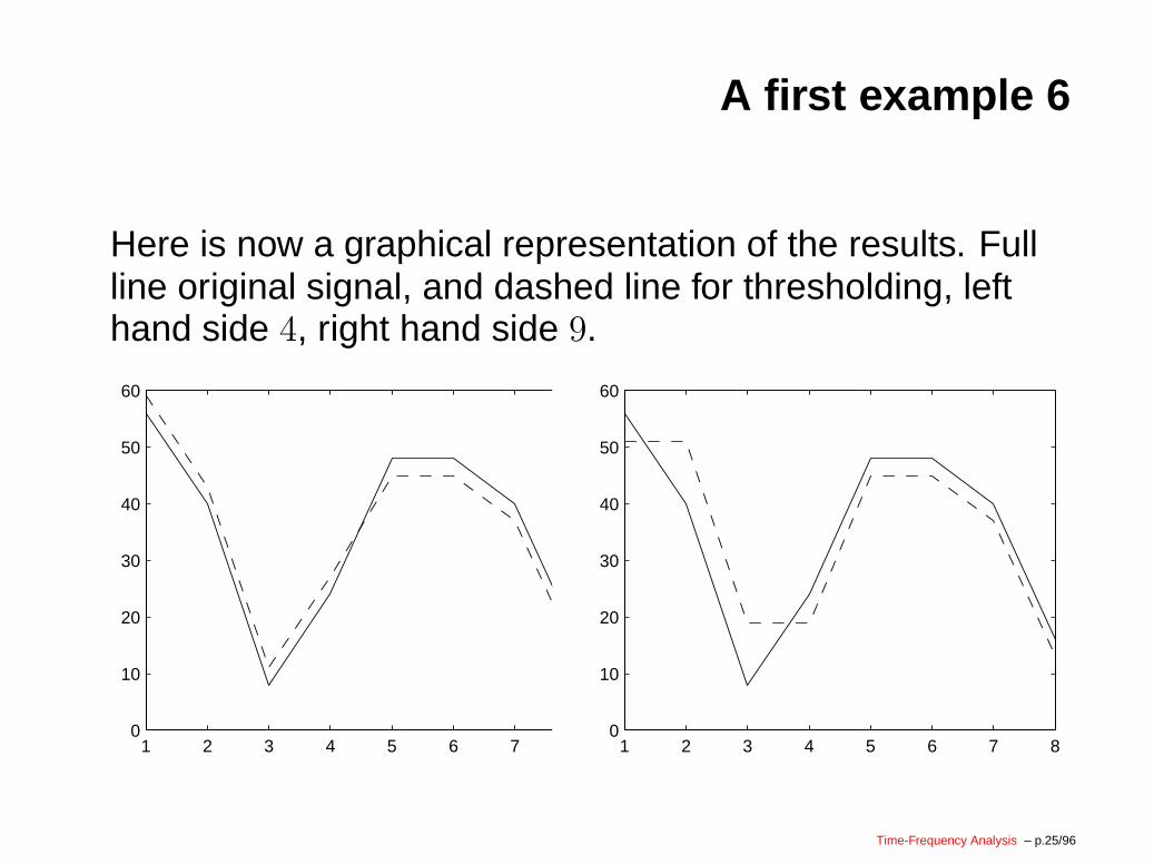
Here is now a graphical representation of the results. Fullline original signal, and dashed line for thresholding, lefthand side 4, right hand side 9.
1 2 3 4 5 6 7 80
10
20
30
40
50
60
1 2 3 4 5 6 7 80
10
20
30
40
50
60
Time-Frequency Analysis – p.25/96
Lifting 1
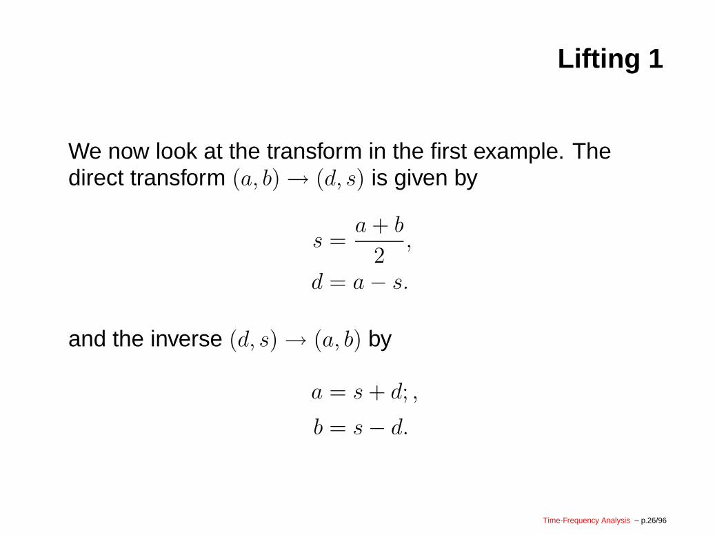
We now look at the transform in the first example. Thedirect transform (a, b)→ (d, s) is given by
s =a + b
2,
d = a− s.
and the inverse (d, s)→ (a, b) by
a = s + d; ,
b = s− d.
Time-Frequency Analysis – p.26/96
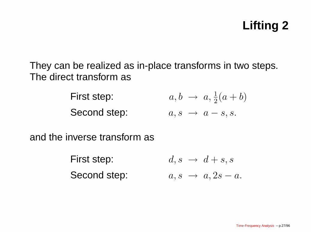
Lifting 2
They can be realized as in-place transforms in two steps.The direct transform as
First step: a, b → a, 12(a + b)
Second step: a, s → a− s, s.
and the inverse transform as
First step: d, s → d + s, s
Second step: a, s → a, 2s− a.
Time-Frequency Analysis – p.27/96
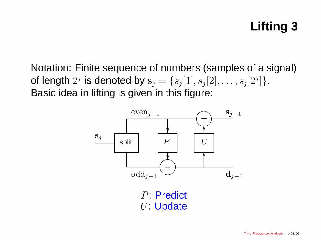
Lifting 3
Notation: Finite sequence of numbers (samples of a signal)of length 2j is denoted by sj = {sj [1], sj [2], . . . , sj [2
j ]}.Basic idea in lifting is given in this figure:
evenj−1
oddj−1
−
sj−1
dj−1
split P Usj
+
P : PredictU : Update
Time-Frequency Analysis – p.28/96
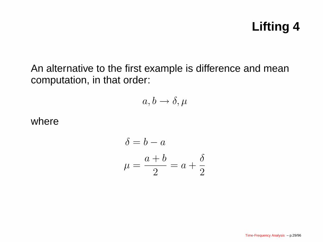
Lifting 4
An alternative to the first example is difference and meancomputation, in that order:
a, b→ δ, µ
where
δ = b− a
µ =a + b
2= a +
δ
2
Time-Frequency Analysis – p.29/96
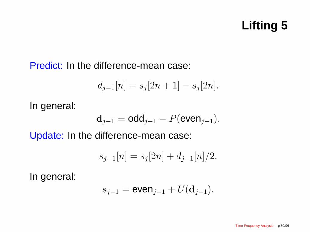
Lifting 5
Predict: In the difference-mean case:
dj−1[n] = sj [2n + 1]− sj [2n].
In general:dj−1 = oddj−1 − P (evenj−1).
Update: In the difference-mean case:
sj−1[n] = sj [2n] + dj−1[n]/2.
In general:sj−1 = evenj−1 + U(dj−1).
Time-Frequency Analysis – p.30/96
Lifting 6
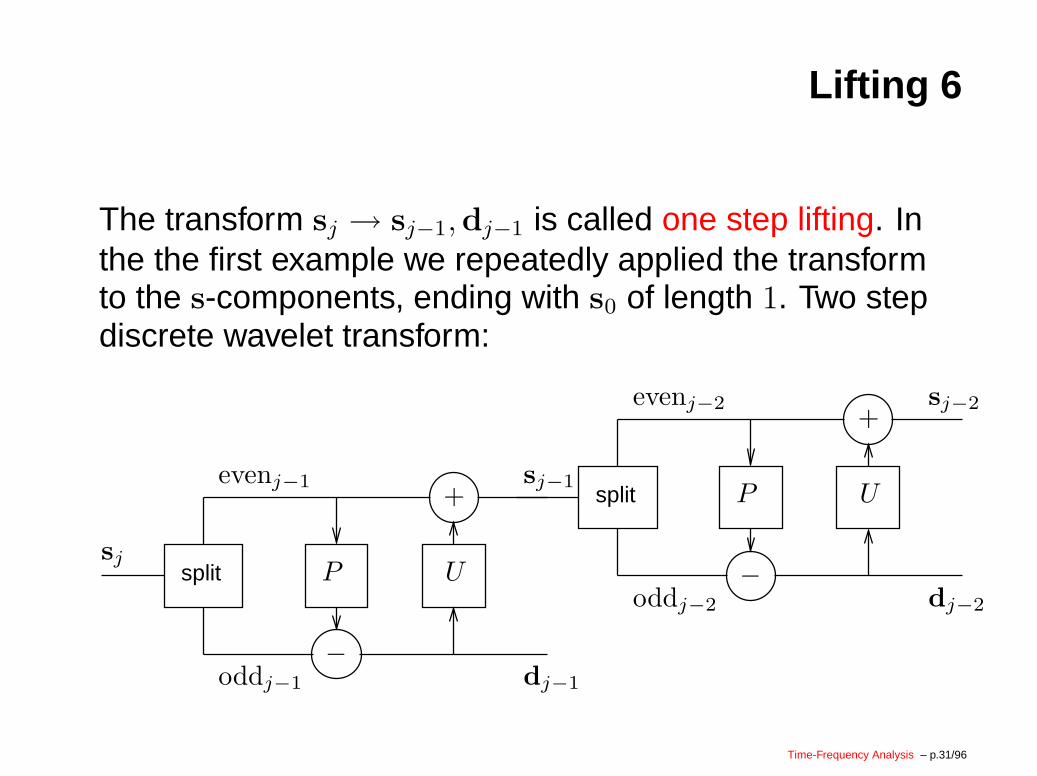
The transform sj → sj−1,dj−1 is called one step lifting. Inthe the first example we repeatedly applied the transformto the s-components, ending with s0 of length 1. Two stepdiscrete wavelet transform:
evenj−1
oddj−1
−
sj−1
dj−1
split P Usj
+
evenj−2
oddj−2
−dj−2
split P U
+sj−2
Time-Frequency Analysis – p.31/96
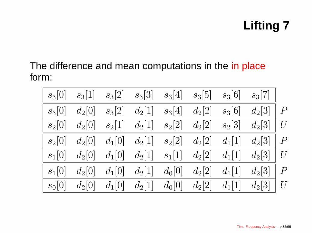
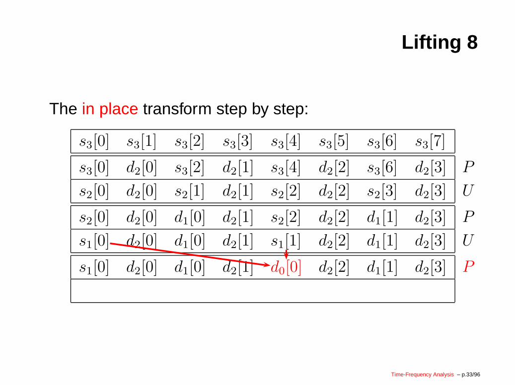
Lifting 7
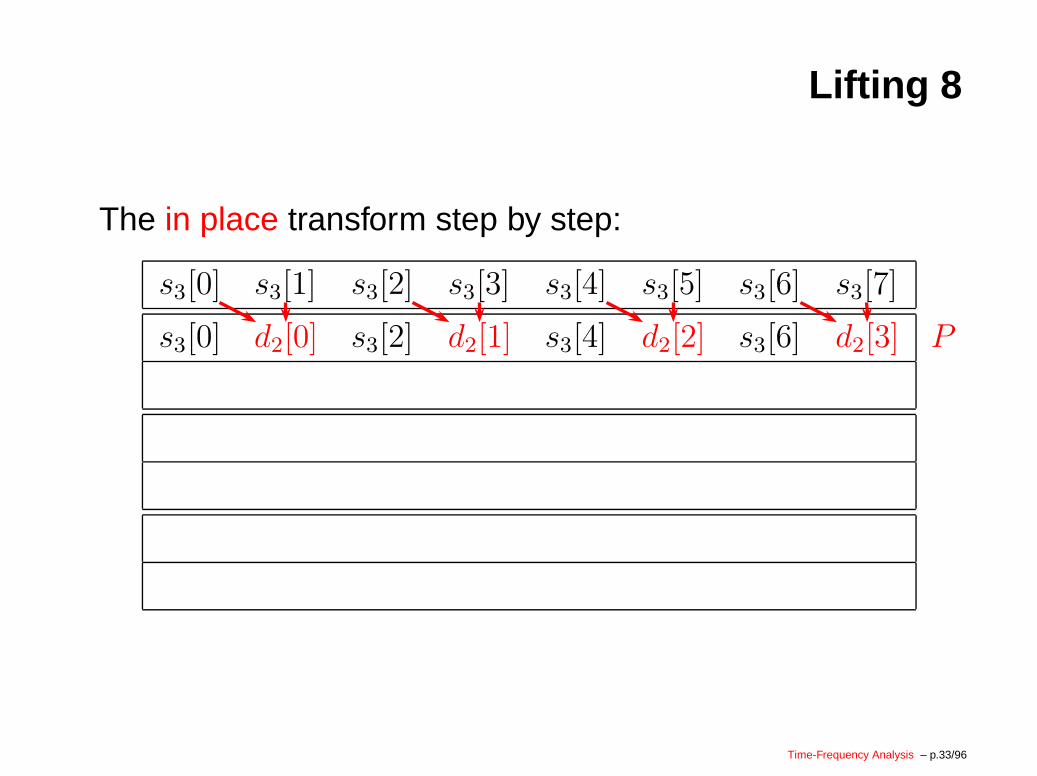
The difference and mean computations in the in placeform:
s3[0] s3[1] s3[2] s3[3] s3[4] s3[5] s3[6] s3[7]
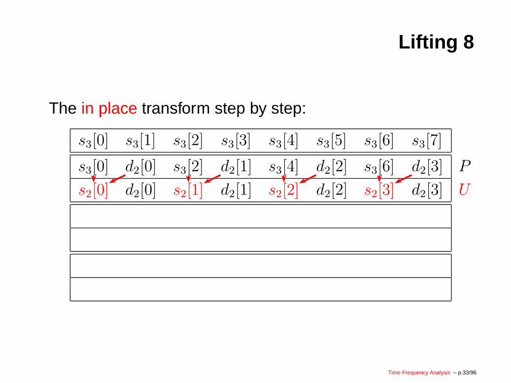
s3[0] d2[0] s3[2] d2[1] s3[4] d2[2] s3[6] d2[3] P
s2[0] d2[0] s2[1] d2[1] s2[2] d2[2] s2[3] d2[3] U
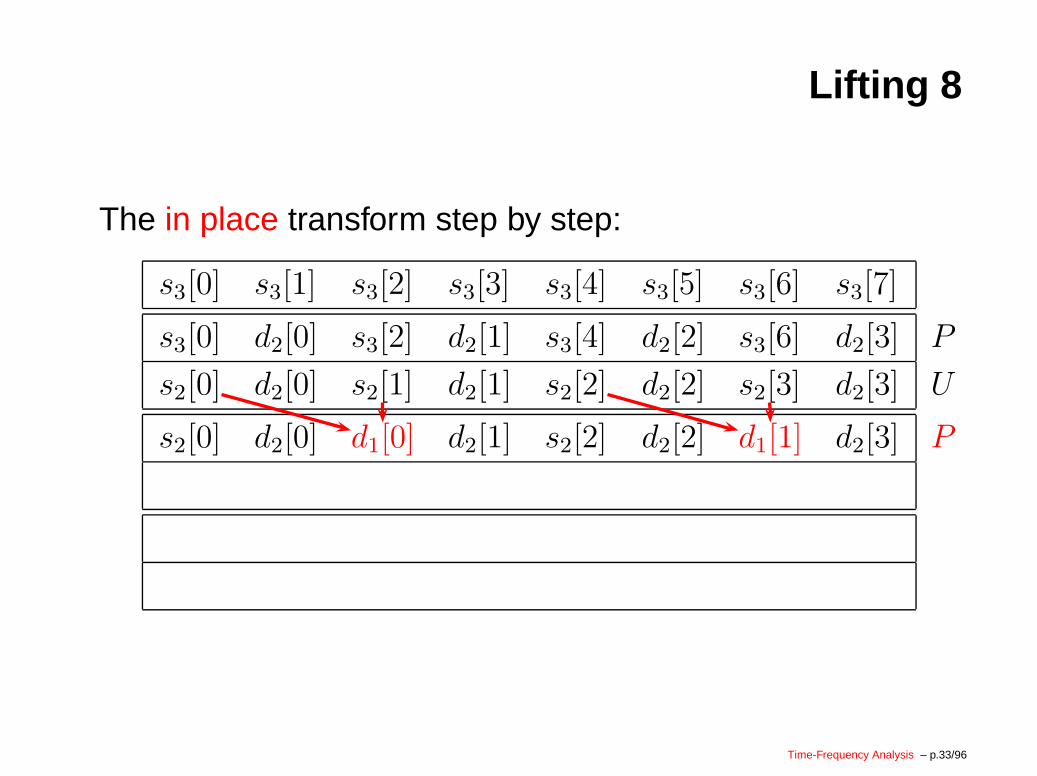
s2[0] d2[0] d1[0] d2[1] s2[2] d2[2] d1[1] d2[3] P
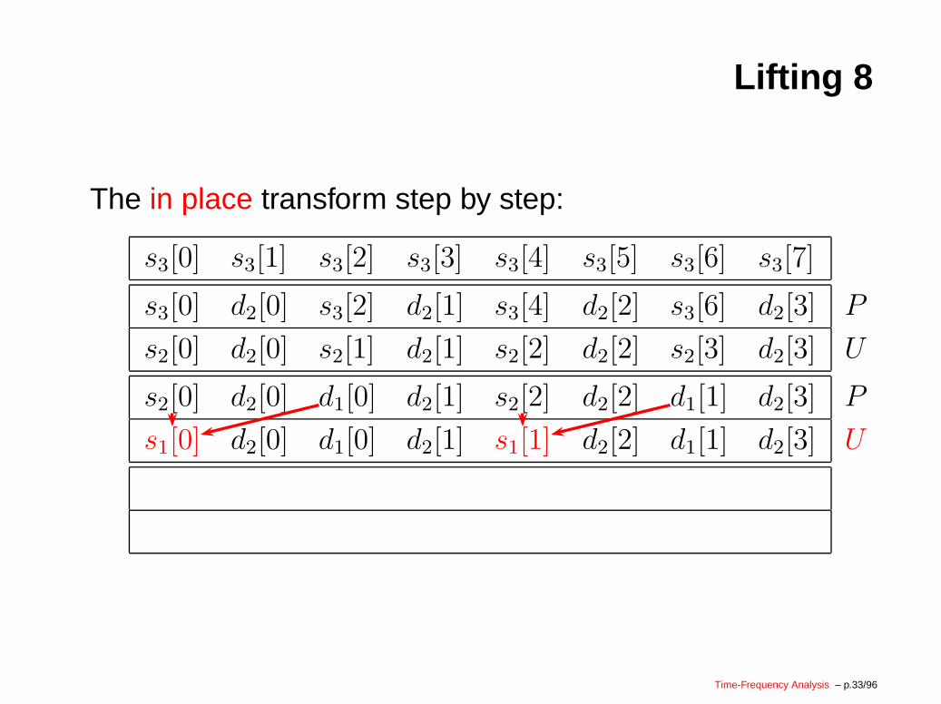
s1[0] d2[0] d1[0] d2[1] s1[1] d2[2] d1[1] d2[3] U
s1[0] d2[0] d1[0] d2[1] d0[0] d2[2] d1[1] d2[3] P
s0[0] d2[0] d1[0] d2[1] d0[0] d2[2] d1[1] d2[3] U
Time-Frequency Analysis – p.32/96
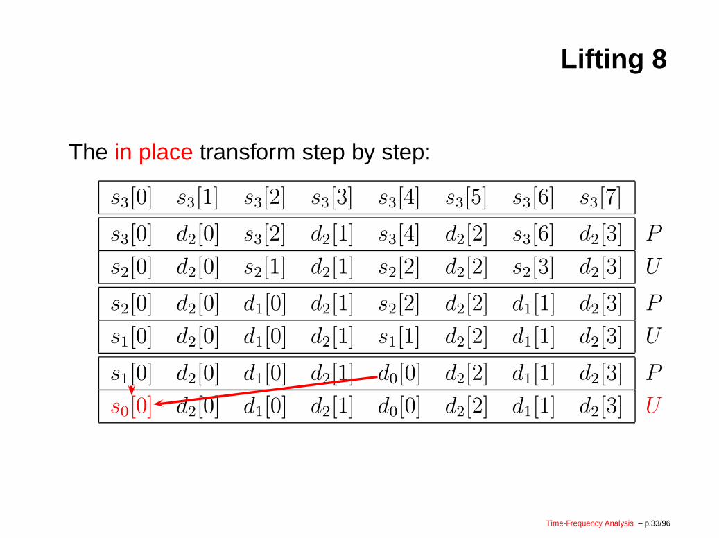
Lifting 8
The in place transform step by step:
Time-Frequency Analysis – p.33/96
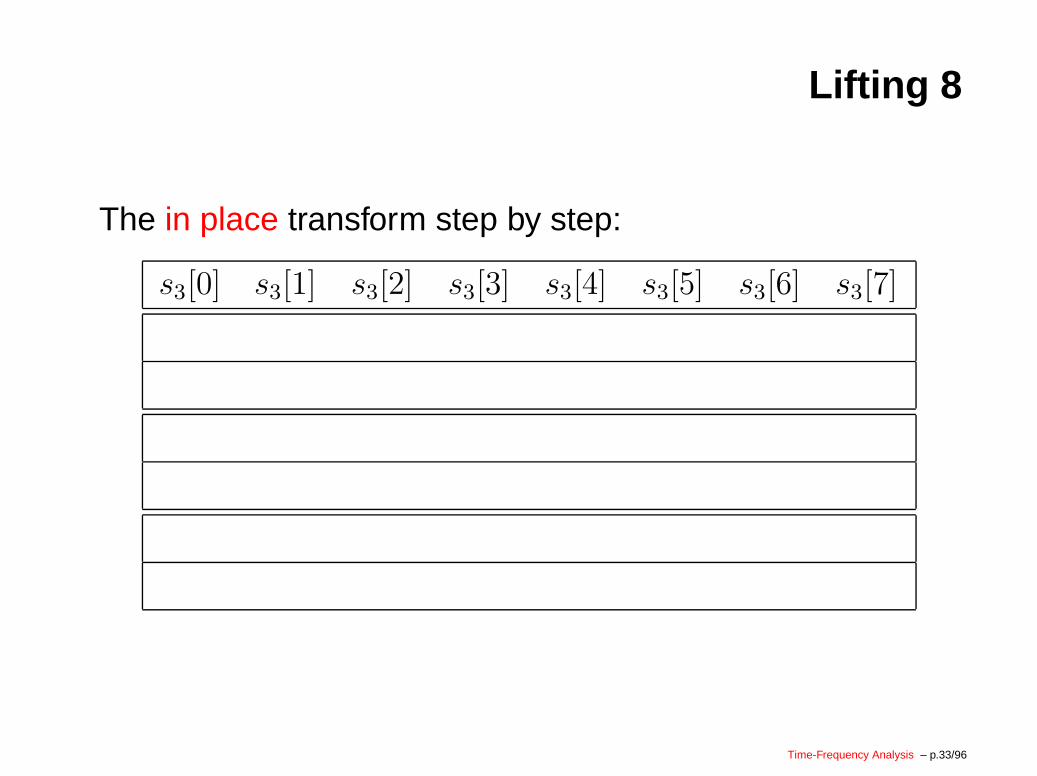
Lifting 8
The in place transform step by step:
s3[0] s3[1] s3[2] s3[3] s3[4] s3[5] s3[6] s3[7]
Time-Frequency Analysis – p.33/96
Lifting 8
The in place transform step by step:
s3[0] s3[1] s3[2] s3[3] s3[4] s3[5] s3[6] s3[7]
s3[0] d2[0] s3[2] d2[1] s3[4] d2[2] s3[6] d2[3] P
Time-Frequency Analysis – p.33/96
Lifting 8
The in place transform step by step:
s3[0] s3[1] s3[2] s3[3] s3[4] s3[5] s3[6] s3[7]
s3[0] d2[0] s3[2] d2[1] s3[4] d2[2] s3[6] d2[3] P
s2[0] d2[0] s2[1] d2[1] s2[2] d2[2] s2[3] d2[3] U
Time-Frequency Analysis – p.33/96
Lifting 8
The in place transform step by step:
s3[0] s3[1] s3[2] s3[3] s3[4] s3[5] s3[6] s3[7]
s3[0] d2[0] s3[2] d2[1] s3[4] d2[2] s3[6] d2[3] P
s2[0] d2[0] s2[1] d2[1] s2[2] d2[2] s2[3] d2[3] U
s2[0] d2[0] d1[0] d2[1] s2[2] d2[2] d1[1] d2[3] P
Time-Frequency Analysis – p.33/96
Lifting 8
The in place transform step by step:
s3[0] s3[1] s3[2] s3[3] s3[4] s3[5] s3[6] s3[7]
s3[0] d2[0] s3[2] d2[1] s3[4] d2[2] s3[6] d2[3] P
s2[0] d2[0] s2[1] d2[1] s2[2] d2[2] s2[3] d2[3] U
s2[0] d2[0] d1[0] d2[1] s2[2] d2[2] d1[1] d2[3] P
s1[0] d2[0] d1[0] d2[1] s1[1] d2[2] d1[1] d2[3] U
s1[0] d2[0] d1[0] d2[1] d0[0] d2[2] d1[1] d2[3] P
s0[0] d2[0] d1[0] d2[1] d0[0] d2[2] d1[1] d2[3] U
Time-Frequency Analysis – p.33/96
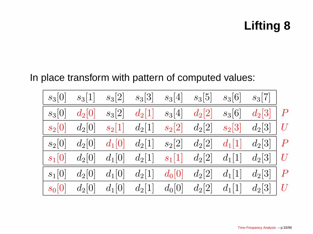
Lifting 8
The in place transform step by step:
In place transform with pattern of computed values:
s3[0] s3[1] s3[2] s3[3] s3[4] s3[5] s3[6] s3[7]
s3[0] d2[0] s3[2] d2[1] s3[4] d2[2] s3[6] d2[3] P
s2[0] d2[0] s2[1] d2[1] s2[2] d2[2] s2[3] d2[3] U
s2[0] d2[0] d1[0] d2[1] s2[2] d2[2] d1[1] d2[3] P
s1[0] d2[0] d1[0] d2[1] s1[1] d2[2] d1[1] d2[3] U
s1[0] d2[0] d1[0] d2[1] d0[0] d2[2] d1[1] d2[3] P
s0[0] d2[0] d1[0] d2[1] d0[0] d2[2] d1[1] d2[3] U
Time-Frequency Analysis – p.33/96
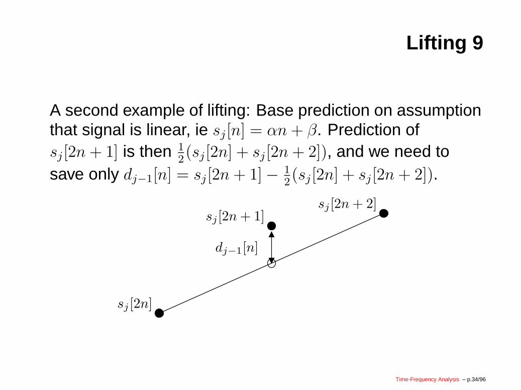
Lifting 9
A second example of lifting: Base prediction on assumptionthat signal is linear, ie sj [n] = αn + β. Prediction ofsj [2n + 1] is then 1
2(sj [2n] + sj [2n + 2]), and we need to
save only dj−1[n] = sj [2n + 1]− 12(sj [2n] + sj [2n + 2]).
dj−1[n]
sj [2n + 1]
sj [2n]
sj [2n + 2]
Time-Frequency Analysis – p.34/96
Lifting 10
The update step: Keep mean of sj [n] sequence equal tomean of sj−1[n] sequence. Final result is
dj−1[n] = sj [2n + 1]− 12(sj[2n] + sj [2n + 2]),
sj−1[n] = sj [2n] + 14(dj−1[n− 1] + dj−1[n]).
Inverse transform:
sj [2n] = sj−1[n]− 14(dj−1[n− 1] + dj−1[n]),
sj [2n + 1] = dj−1[n] + 12(sj [2n] + sj [2n + 2]).
Time-Frequency Analysis – p.35/96
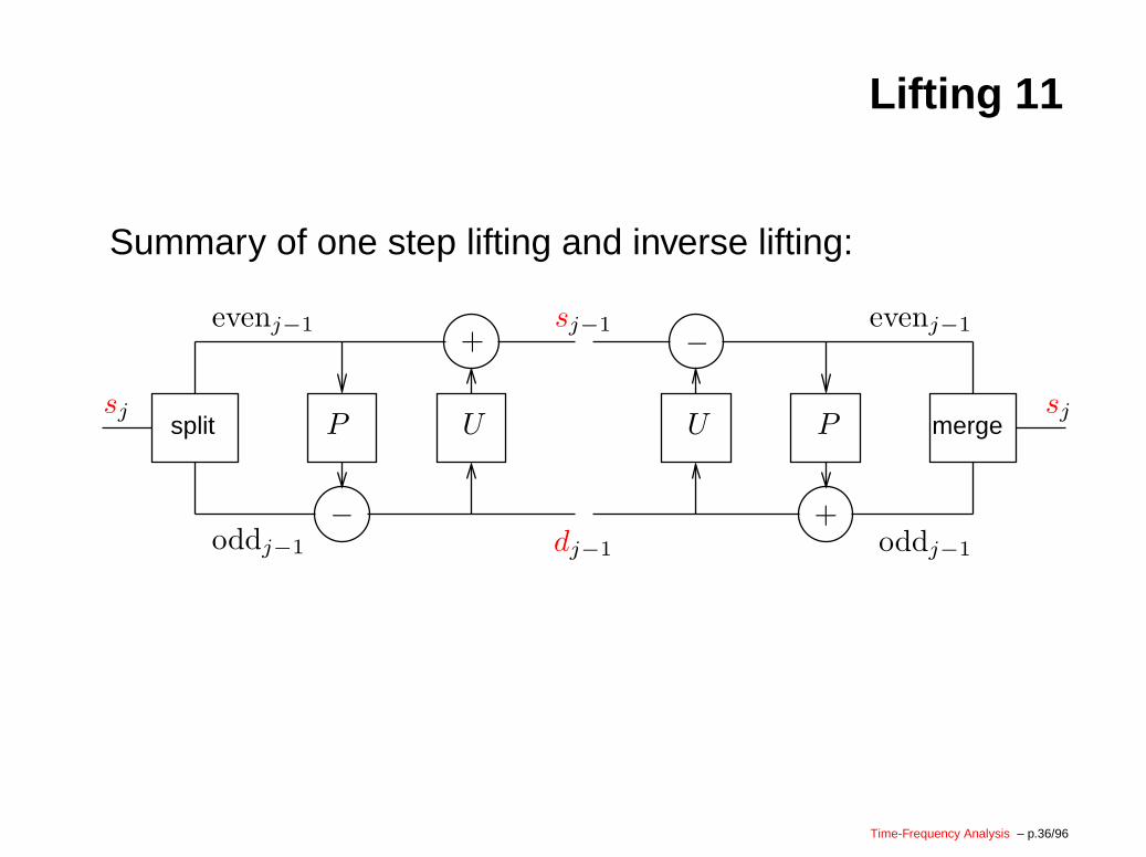
Lifting 11
Summary of one step lifting and inverse lifting:
PU
+
−
merge
evenj−1
oddj−1
−
split P U
+
dj−1
sj−1 evenj−1
oddj−1
sjsj
Time-Frequency Analysis – p.36/96
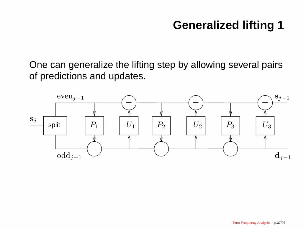
Generalized lifting 1
One can generalize the lifting step by allowing several pairsof predictions and updates.
−
split P1 U1
sj
+
oddj−1
evenj−1
dj−1
−
P3 U3
+
−
P2 U2
+sj−1
Time-Frequency Analysis – p.37/96
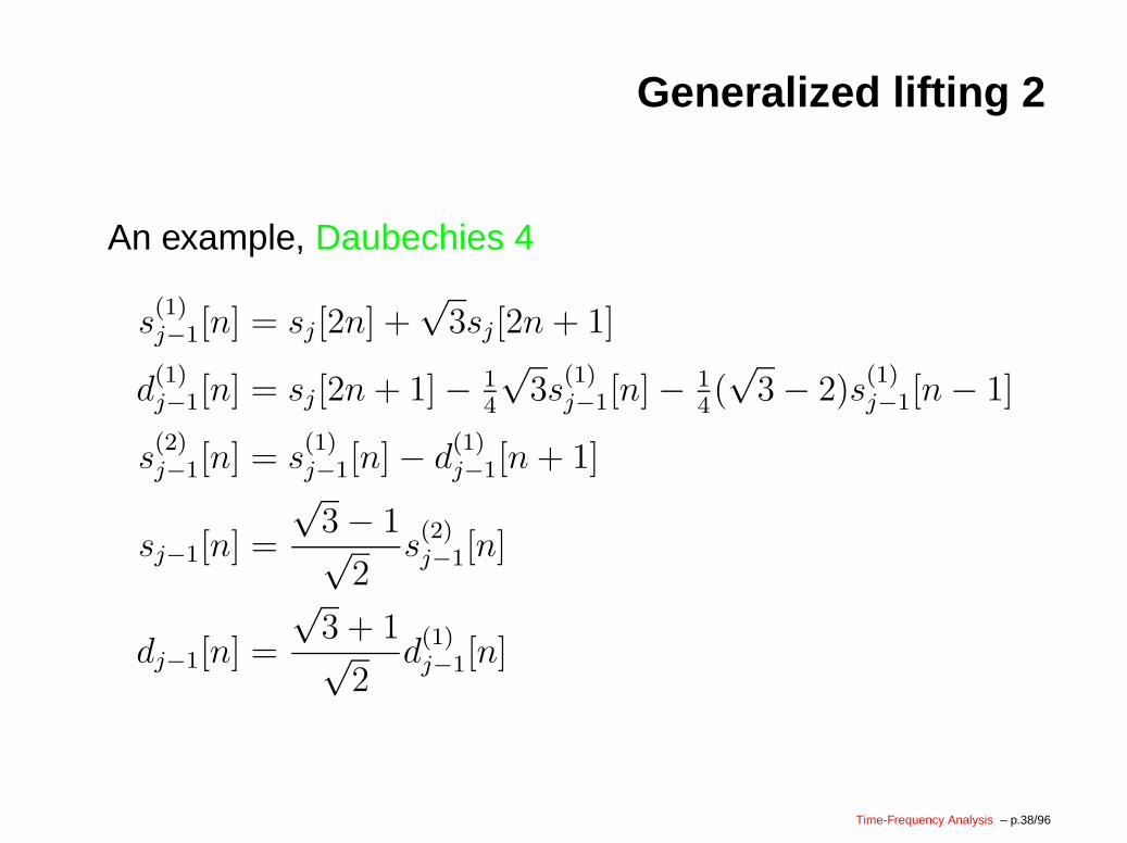
Generalized lifting 2
An example, Daubechies 4
s(1)j−1[n] = sj [2n] +
√3sj [2n + 1]
d(1)j−1[n] = sj [2n + 1]− 1
4
√3s
(1)j−1[n]− 1
4(√
3− 2)s(1)j−1[n− 1]
s(2)j−1[n] = s
(1)j−1[n]− d
(1)j−1[n + 1]
sj−1[n] =
√3− 1√
2s(2)j−1[n]
dj−1[n] =
√3 + 1√
2d
(1)j−1[n]
Time-Frequency Analysis – p.38/96
Generalized lifting 3
Last two steps are normalization steps, in order topreserve the energy in the transform, ie
∑
n
|sj [n]|2 =∑
n
|sj−1[n]|2 +∑
n
|dj−1[n]|2
now holds. Note that√
3− 1√2·√
3 + 1√2
= 1 .
Time-Frequency Analysis – p.39/96
DWT 1
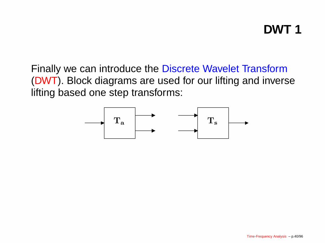
Finally we can introduce the Discrete Wavelet Transform(DWT). Block diagrams are used for our lifting and inverselifting based one step transforms:
Ta Ts
Time-Frequency Analysis – p.40/96
DWT 2
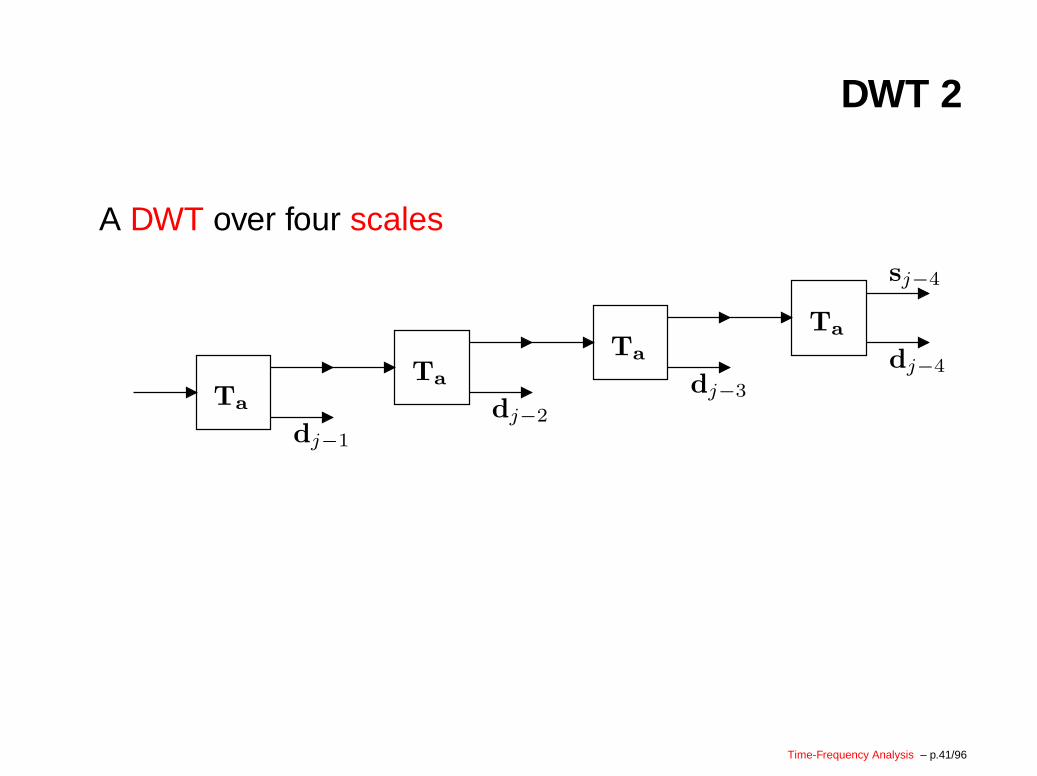
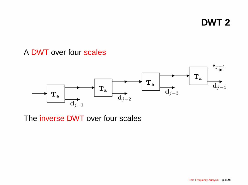
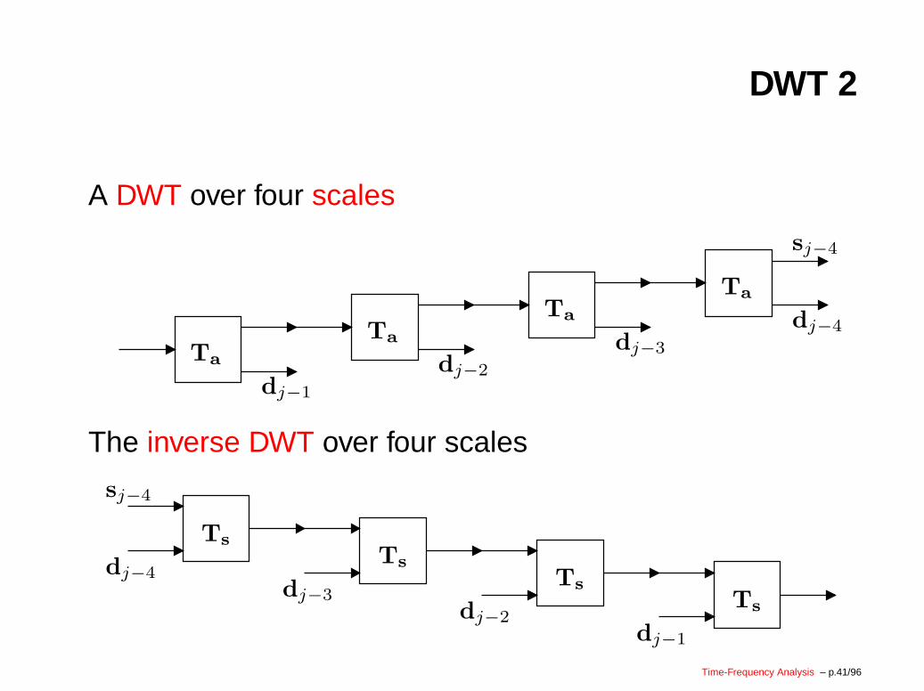
A DWT over four scales
Ta
dj−1
Ta
dj−2
Ta
dj−3
Ta
dj−4
sj−4
The inverse DWT over four scales
dj−3
dj−4
sj−4
dj−2dj−1
Ts
Ts
Ts
Ts
Time-Frequency Analysis – p.41/96
DWT 2
A DWT over four scales
Ta
dj−1
Ta
dj−2
Ta
dj−3
Ta
dj−4
sj−4
The inverse DWT over four scales
dj−3
dj−4
sj−4
dj−2dj−1
Ts
Ts
Ts
Ts
Time-Frequency Analysis – p.41/96
DWT 2
A DWT over four scales
Ta
dj−1
Ta
dj−2
Ta
dj−3
Ta
dj−4
sj−4
The inverse DWT over four scales
dj−3
dj−4
sj−4
dj−2dj−1
Ts
Ts
Ts
Ts
Time-Frequency Analysis – p.41/96
DWT 2
A DWT over four scales
Ta
dj−1
Ta
dj−2
Ta
dj−3
Ta
dj−4
sj−4
The inverse DWT over four scales
dj−3
dj−4
sj−4
dj−2dj−1
Ts
Ts
Ts
Ts
Time-Frequency Analysis – p.41/96
DWT 3
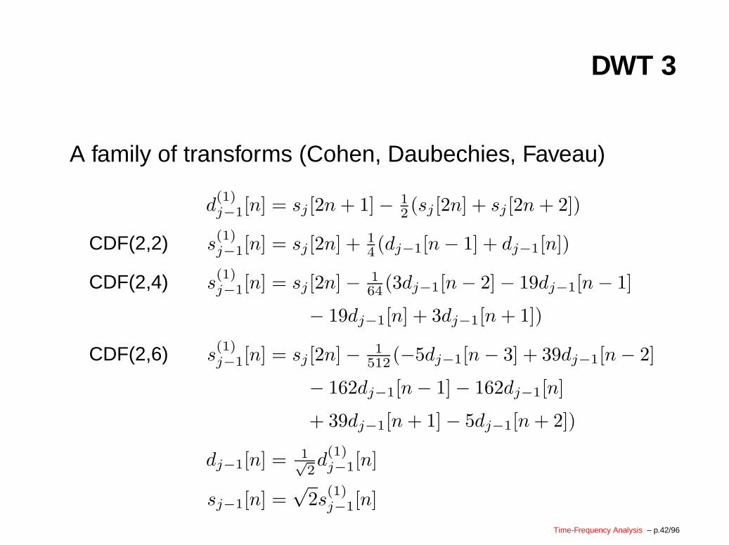
A family of transforms (Cohen, Daubechies, Faveau)
d(1)j−1[n] = sj [2n + 1]− 1
2(sj [2n] + sj [2n + 2])
CDF(2,2) s(1)j−1[n] = sj [2n] + 1
4 (dj−1[n− 1] + dj−1[n])
CDF(2,4) s(1)j−1[n] = sj [2n]− 1
64 (3dj−1[n− 2]− 19dj−1[n− 1]
− 19dj−1[n] + 3dj−1[n + 1])
CDF(2,6) s(1)j−1[n] = sj [2n]− 1
512 (−5dj−1[n− 3] + 39dj−1[n− 2]
− 162dj−1[n− 1]− 162dj−1[n]
+ 39dj−1[n + 1]− 5dj−1[n + 2])
dj−1[n] = 1√
2d(1)j−1[n]
sj−1[n] =√
2s(1)j−1[n]
Time-Frequency Analysis – p.42/96
Examples 1
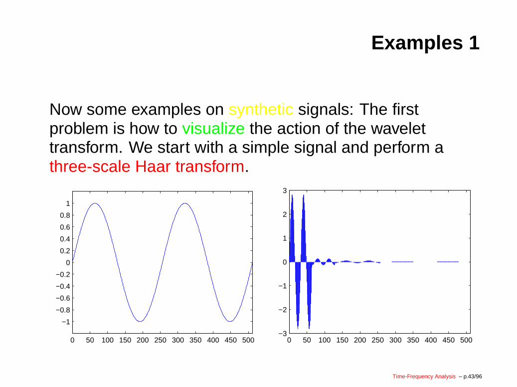
Now some examples on synthetic signals: The firstproblem is how to visualize the action of the wavelettransform. We start with a simple signal and perform athree-scale Haar transform.
0 50 100 150 200 250 300 350 400 450 500
−1
−0.8
−0.6
−0.4
−0.2
0
0.2
0.4
0.6
0.8
1
0 50 100 150 200 250 300 350 400 450 500−3
−2
−1
0
1
2
3
Time-Frequency Analysis – p.43/96
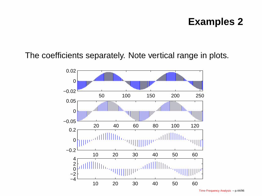
Examples 2
The coefficients separately. Note vertical range in plots.
10 20 30 40 50 60−4−2
024
10 20 30 40 50 60−0.2
0
0.220 40 60 80 100 120
−0.05
0
0.0550 100 150 200 250
−0.02
0
0.02
Time-Frequency Analysis – p.44/96
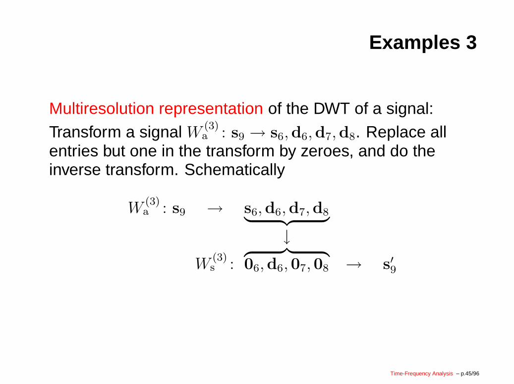
Examples 3
Multiresolution representation of the DWT of a signal:Transform a signal W
(3)a : s9 → s6,d6,d7,d8. Replace all
entries but one in the transform by zeroes, and do theinverse transform. Schematically
W(3)a : s9 → s6,d6,d7,d8
︸ ︷︷ ︸
↓W
(3)s :
︷ ︸︸ ︷
06,d6,07,08 → s′
9
Time-Frequency Analysis – p.45/96
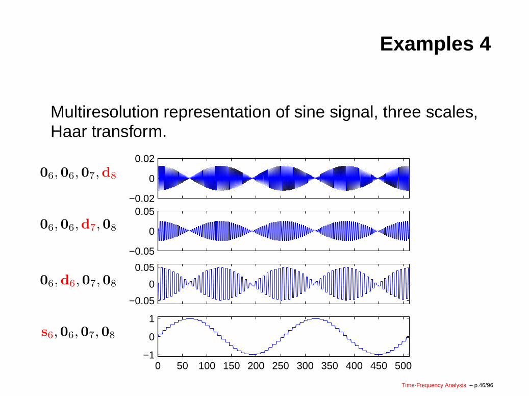
Examples 4
Multiresolution representation of sine signal, three scales,Haar transform.
−0.02
0
0.02
−0.05
0
0.05
−0.05
0
0.05
0 50 100 150 200 250 300 350 400 450 500−1
0
1s6,06,07,08
06,d6,07,08
06,06,d7,08
06,06,07,d8
Time-Frequency Analysis – p.46/96
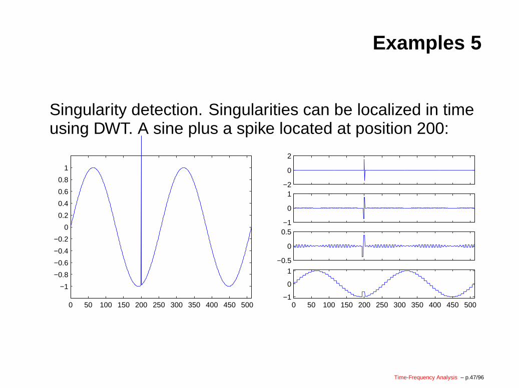
Examples 5
Singularity detection. Singularities can be localized in timeusing DWT. A sine plus a spike located at position 200:
0 50 100 150 200 250 300 350 400 450 500
−1
−0.8
−0.6
−0.4
−0.2
0
0.2
0.4
0.6
0.8
1
−2
0
2
−1
0
1
−0.5
0
0.5
0 50 100 150 200 250 300 350 400 450 500−1
0
1
Time-Frequency Analysis – p.47/96
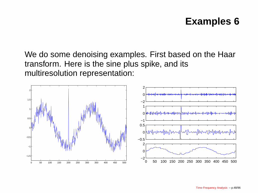
Examples 6
We do some denoising examples. First based on the Haartransform. Here is the sine plus spike, and itsmultiresolution representation:
0 50 100 150 200 250 300 350 400 450 500
−1.5
−1
−0.5
0
0.5
1
1.5
2
−2
0
2
−1
0
1
−0.5
0
0.5
0 50 100 150 200 250 300 350 400 450 500−2
0
2
Time-Frequency Analysis – p.48/96
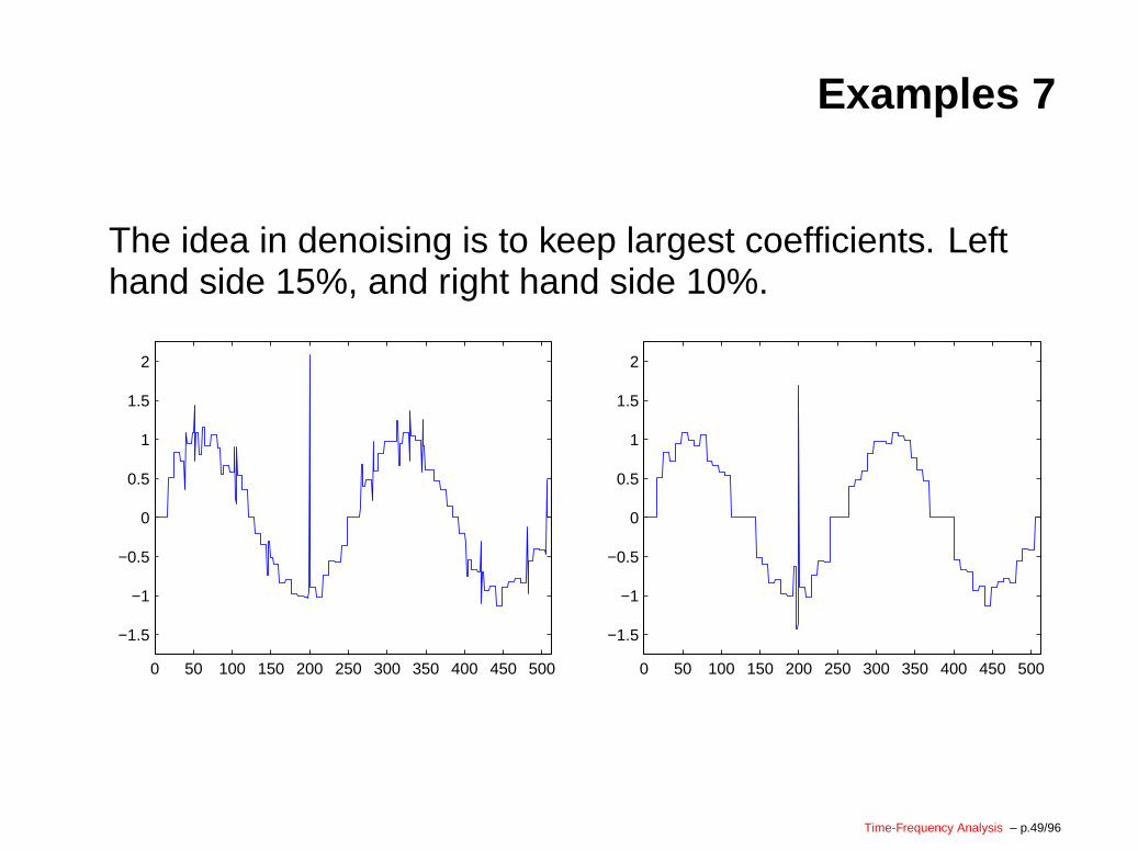
Examples 7
The idea in denoising is to keep largest coefficients. Lefthand side 15%, and right hand side 10%.
0 50 100 150 200 250 300 350 400 450 500
−1.5
−1
−0.5
0
0.5
1
1.5
2
0 50 100 150 200 250 300 350 400 450 500
−1.5
−1
−0.5
0
0.5
1
1.5
2
Time-Frequency Analysis – p.49/96
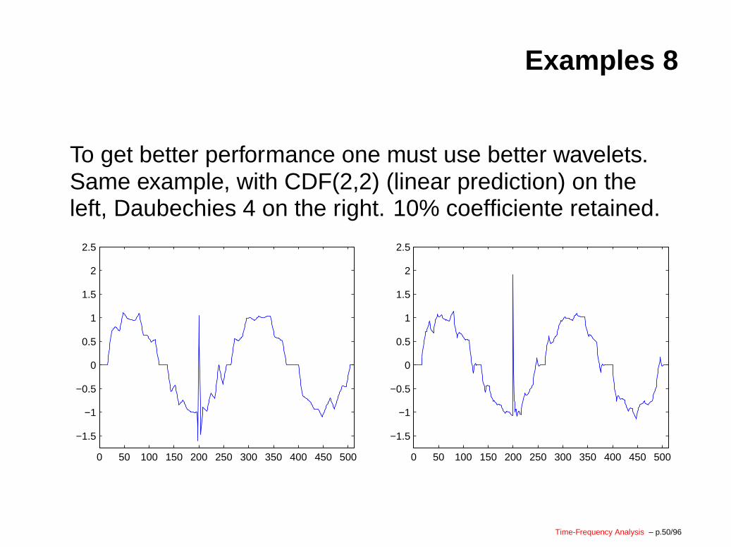
Examples 8
To get better performance one must use better wavelets.Same example, with CDF(2,2) (linear prediction) on theleft, Daubechies 4 on the right. 10% coefficiente retained.
0 50 100 150 200 250 300 350 400 450 500
−1.5
−1
−0.5
0
0.5
1
1.5
2
2.5
0 50 100 150 200 250 300 350 400 450 500
−1.5
−1
−0.5
0
0.5
1
1.5
2
2.5
Time-Frequency Analysis – p.50/96
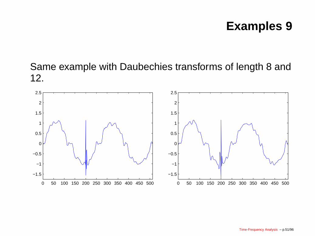
Examples 9
Same example with Daubechies transforms of length 8 and12.
0 50 100 150 200 250 300 350 400 450 500
−1.5
−1
−0.5
0
0.5
1
1.5
2
2.5
0 50 100 150 200 250 300 350 400 450 500
−1.5
−1
−0.5
0
0.5
1
1.5
2
2.5
Time-Frequency Analysis – p.51/96
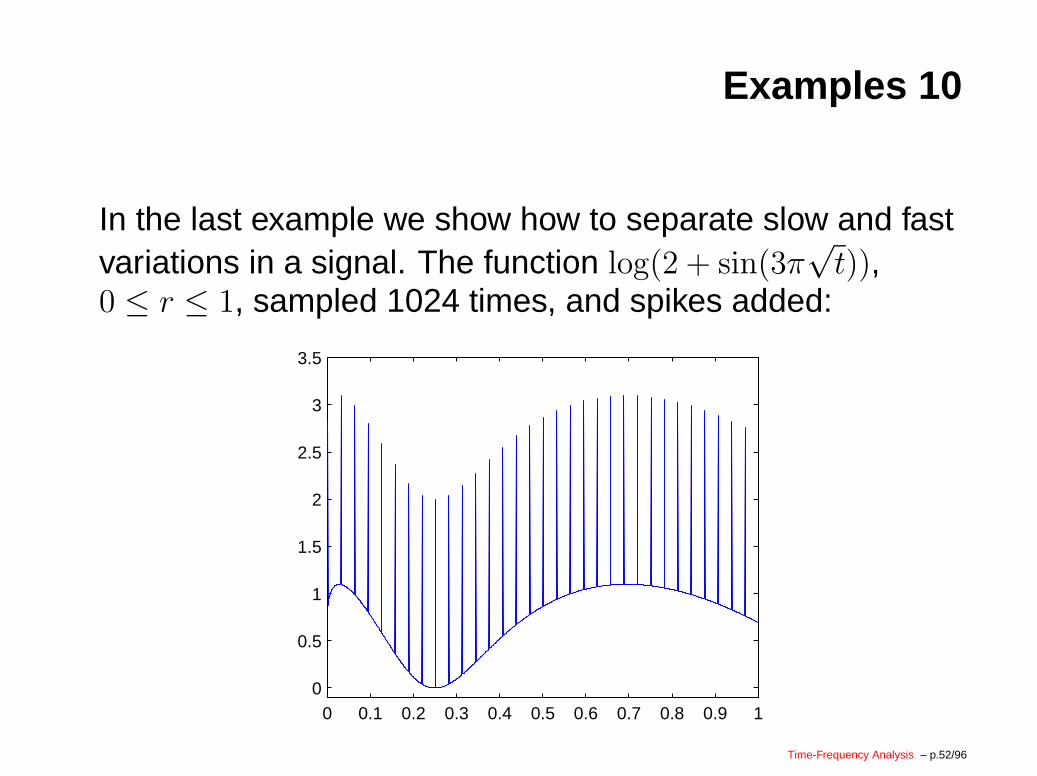
Examples 10
In the last example we show how to separate slow and fastvariations in a signal. The function log(2 + sin(3π
√t)),
0 ≤ r ≤ 1, sampled 1024 times, and spikes added:
0 0.1 0.2 0.3 0.4 0.5 0.6 0.7 0.8 0.9 10
0.5
1
1.5
2
2.5
3
3.5
Time-Frequency Analysis – p.52/96
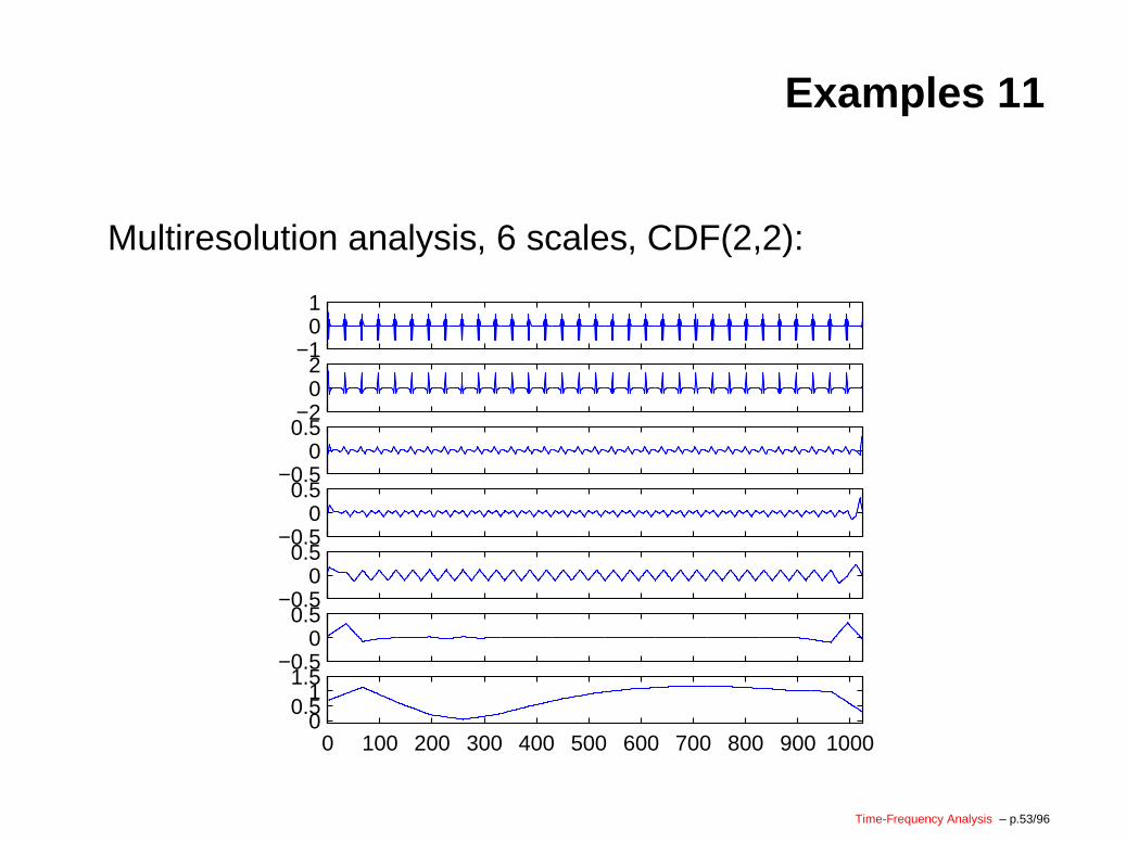
Examples 11
Multiresolution analysis, 6 scales, CDF(2,2):
−101
−202
−0.50
0.5
−0.50
0.5
−0.50
0.5
−0.50
0.5
0 100 200 300 400 500 600 700 800 900 10000
0.51
1.5
Time-Frequency Analysis – p.53/96
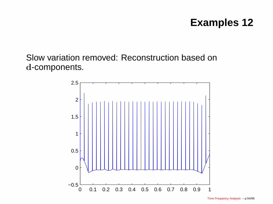
Examples 12
Slow variation removed: Reconstruction based ond-components.
0 0.1 0.2 0.3 0.4 0.5 0.6 0.7 0.8 0.9 1−0.5
0
0.5
1
1.5
2
2.5
Time-Frequency Analysis – p.54/96
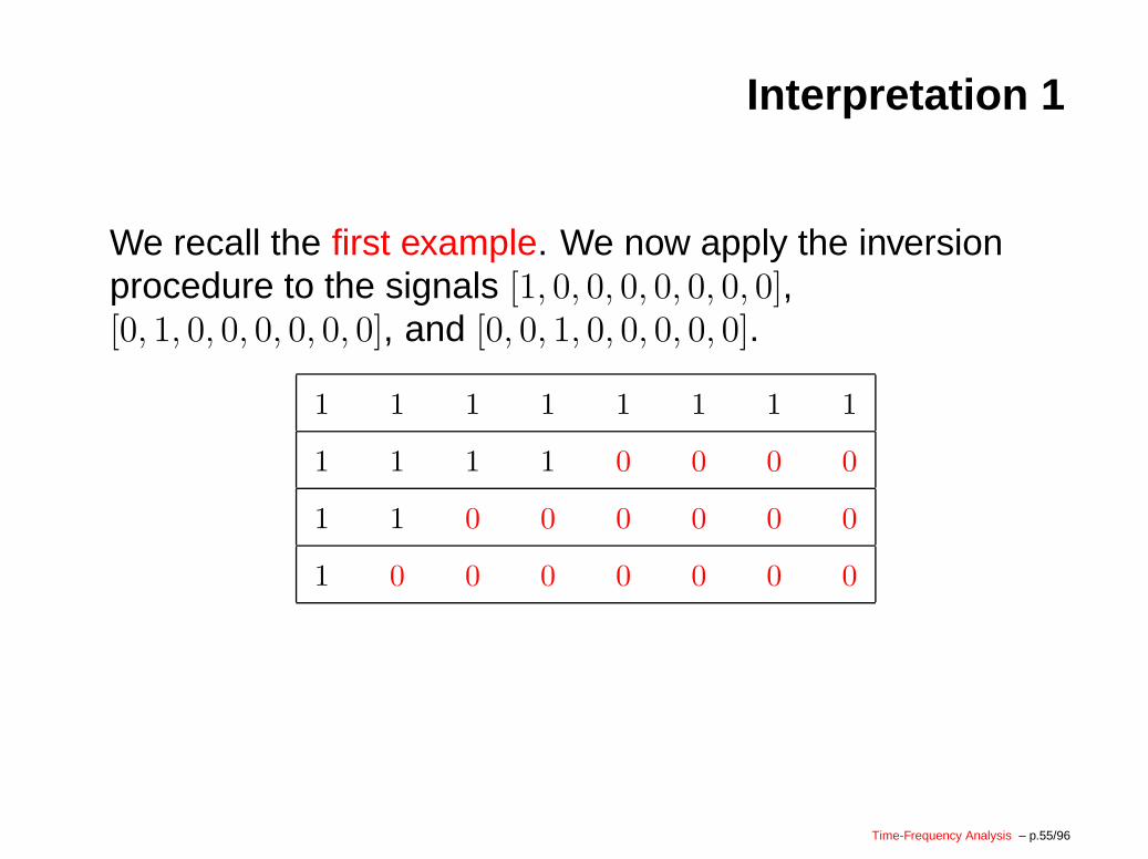
Interpretation 1
We recall the first example. We now apply the inversionprocedure to the signals [1, 0, 0, 0, 0, 0, 0, 0],[0, 1, 0, 0, 0, 0, 0, 0], and [0, 0, 1, 0, 0, 0, 0, 0].
1 1 1 1 1 1 1 1
1 1 1 1 0 0 0 0
1 1 0 0 0 0 0 0
1 0 0 0 0 0 0 0
Time-Frequency Analysis – p.55/96
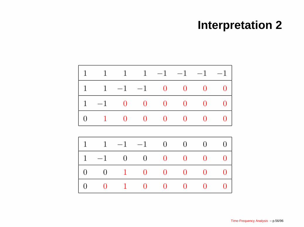
Interpretation 2
1 1 1 1 −1 −1 −1 −1
1 1 −1 −1 0 0 0 0
1 −1 0 0 0 0 0 0
0 1 0 0 0 0 0 0
1 1 −1 −1 0 0 0 0
1 −1 0 0 0 0 0 0
0 0 1 0 0 0 0 0
0 0 1 0 0 0 0 0
Time-Frequency Analysis – p.56/96
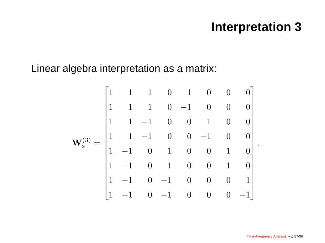
Interpretation 3
Linear algebra interpretation as a matrix:
W(3)s =
1 1 1 0 1 0 0 0
1 1 1 0 −1 0 0 0
1 1 −1 0 0 1 0 0
1 1 −1 0 0 −1 0 0
1 −1 0 1 0 0 1 0
1 −1 0 1 0 0 −1 0
1 −1 0 −1 0 0 0 1
1 −1 0 −1 0 0 0 −1
.
Time-Frequency Analysis – p.57/96
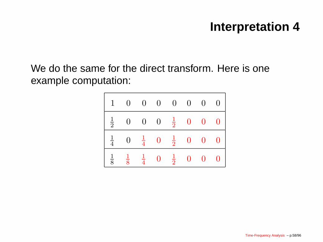
Interpretation 4
We do the same for the direct transform. Here is oneexample computation:
1 0 0 0 0 0 0 0
12 0 0 0 1
2 0 0 0
14 0 1
4 0 12 0 0 0
18
18
14 0 1
2 0 0 0
Time-Frequency Analysis – p.58/96
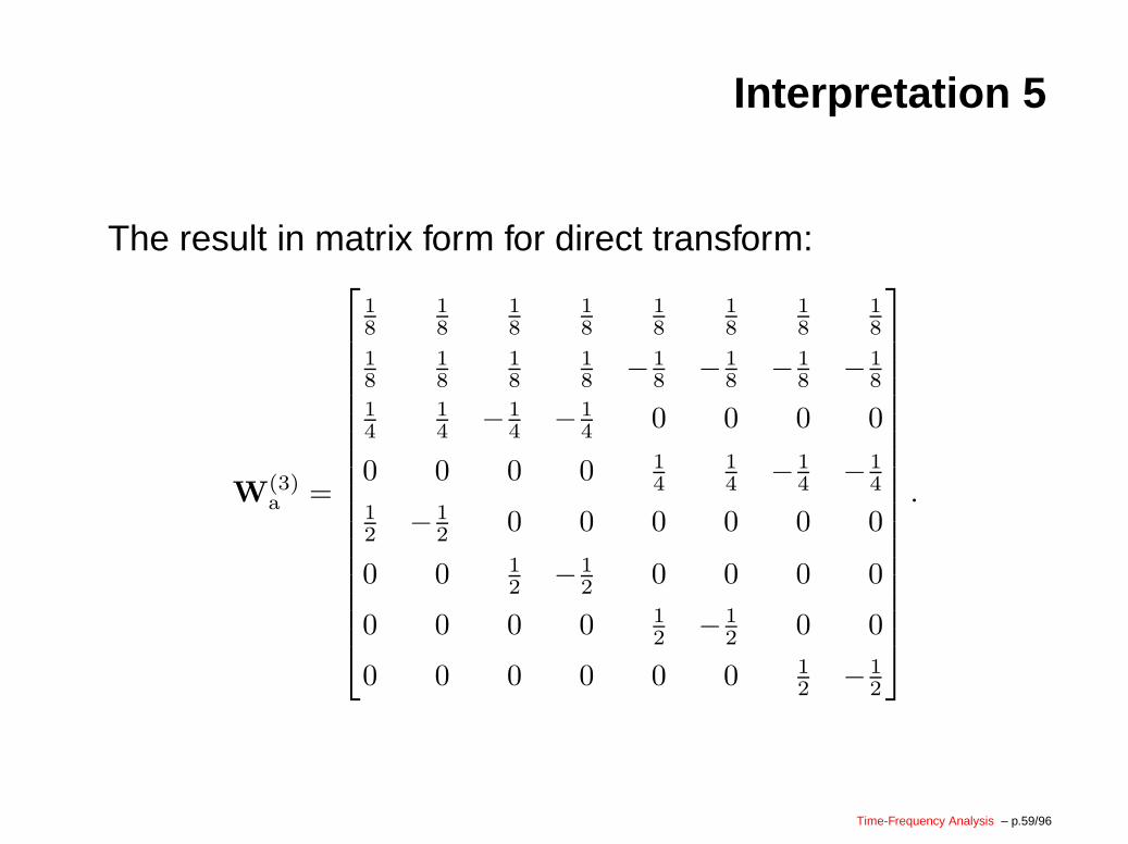
Interpretation 5
The result in matrix form for direct transform:
W(3)a =
18
18
18
18
18
18
18
18
18
18
18
18 − 1
8 − 18 − 1
8 − 18
14
14 − 1
4 − 14 0 0 0 0
0 0 0 0 14
14 − 1
4 − 14
12 − 1
2 0 0 0 0 0 0
0 0 12 − 1
2 0 0 0 0
0 0 0 0 12 − 1
2 0 0
0 0 0 0 0 0 12 − 1
2
.
Time-Frequency Analysis – p.59/96

Interpretation 6
Here is a graphical representation of the contents of W(3)a :
−1
0
1
−1
0
1
−1
0
1
−1
0
1
−1
0
1
−1
0
1
0 0.25 0.5 0.75 1−1
0
1
0 0.25 0.5 0.75 1−1
0
1
Time-Frequency Analysis – p.60/96
Interpretation 6
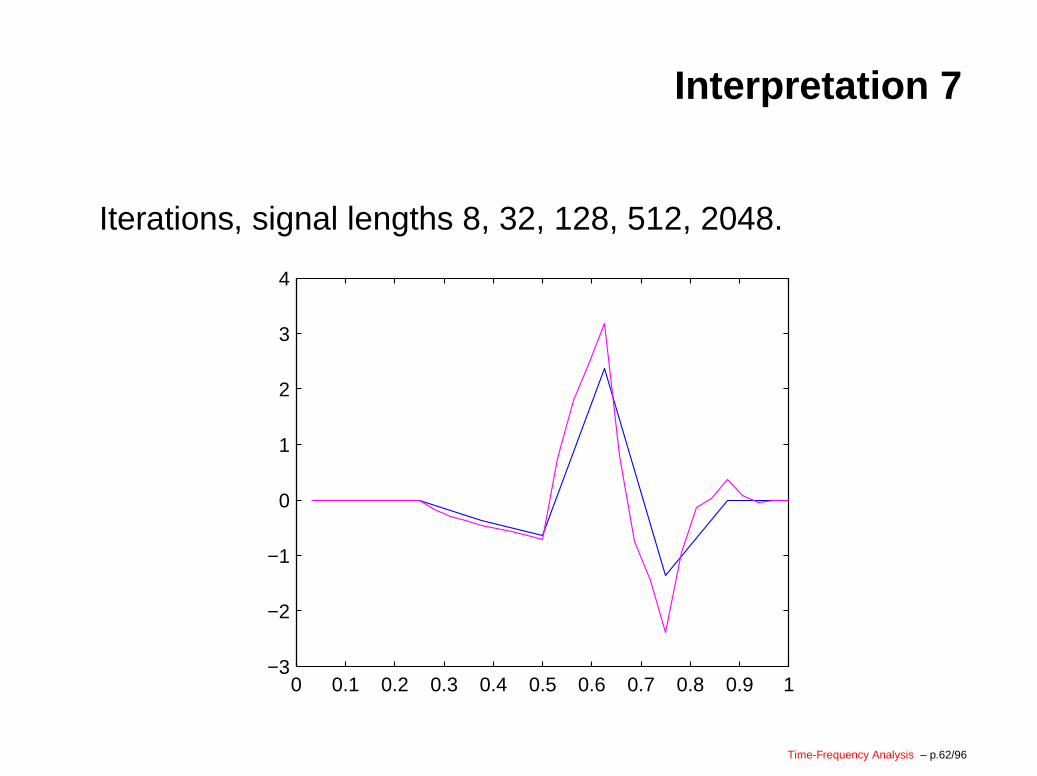
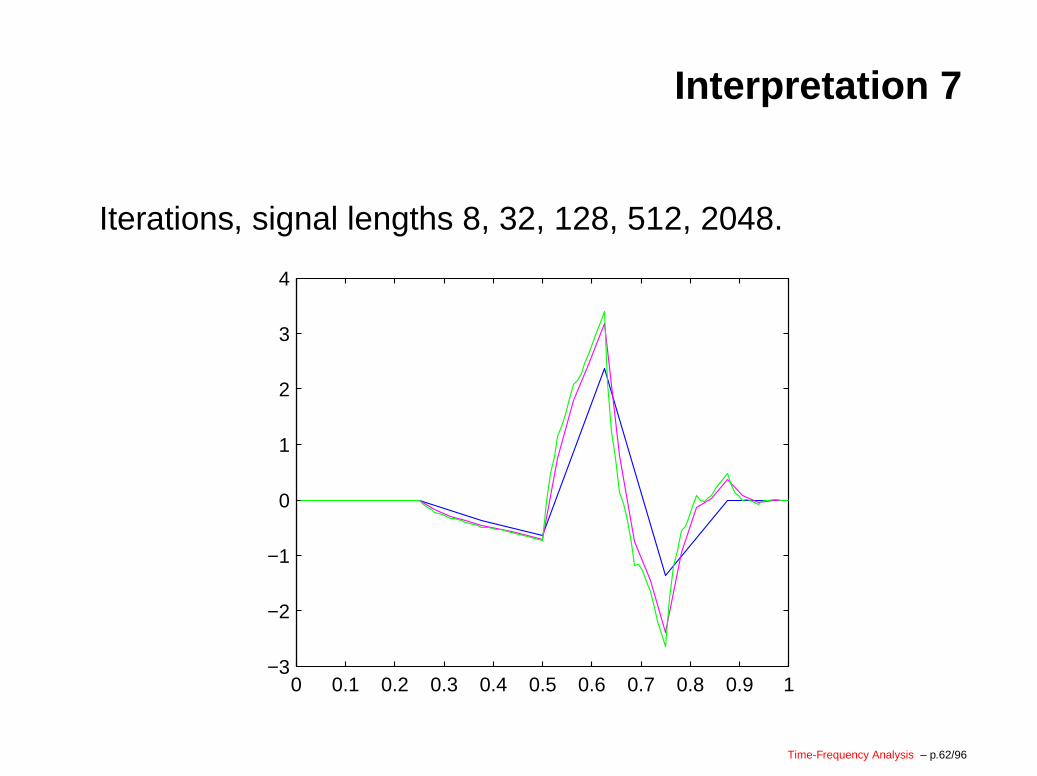
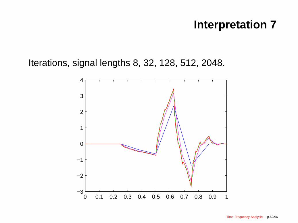
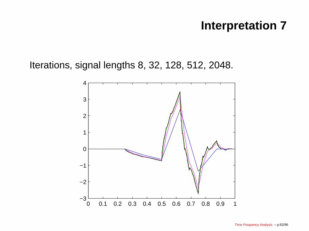
It is one of the nontrivial results in wavelet theory that therealways are either 2 or 4 waveforms behind each DWT.These waveforms get scaled and translated. Byreconstructing from signals with zeroes except a single 1,one can find these waveforms. Here is an example usingthe inverse of the Daubechies 4 transform. We take theinverse transform of a signal with a one at place 6, andtake lengths 8, 32, 128, 512, and 2048. The result isshown on the next slide.
Time-Frequency Analysis – p.61/96
Interpretation 7
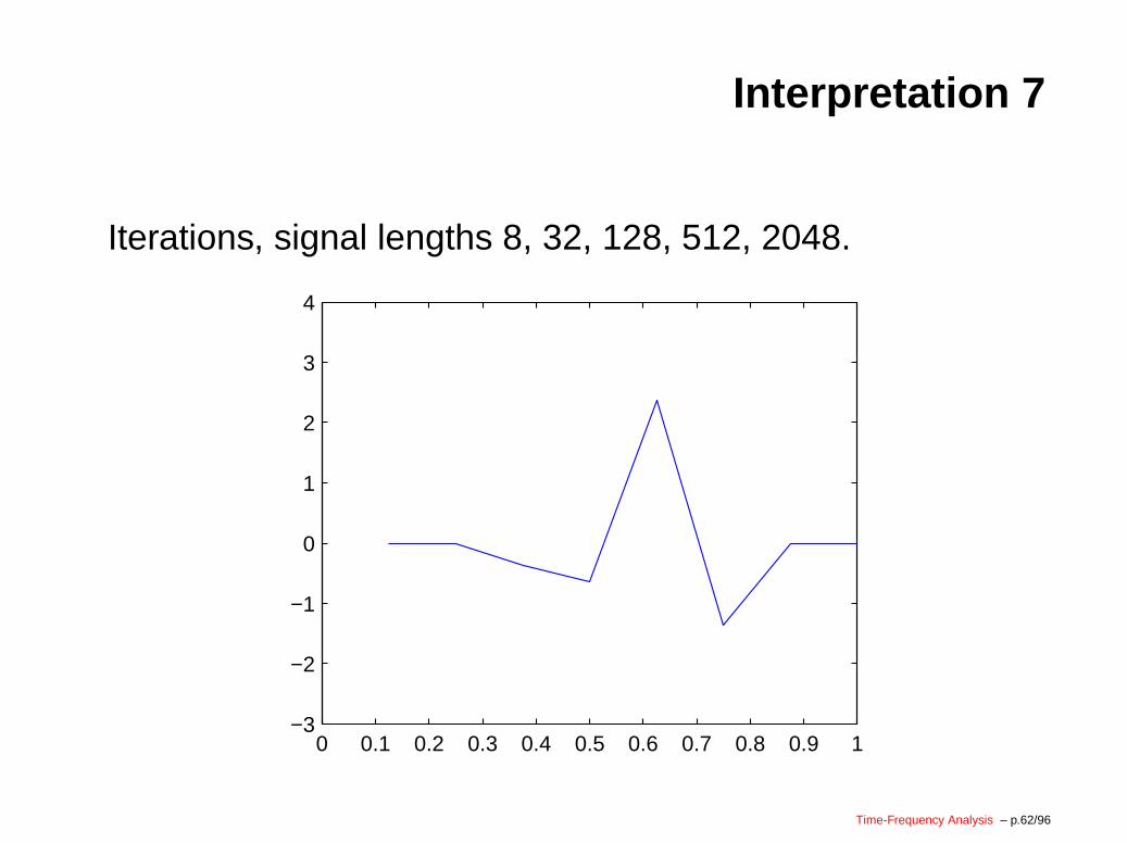
Iterations, signal lengths 8, 32, 128, 512, 2048.
Time-Frequency Analysis – p.62/96
Interpretation 7
Iterations, signal lengths 8, 32, 128, 512, 2048.
0 0.1 0.2 0.3 0.4 0.5 0.6 0.7 0.8 0.9 1−3
−2
−1
0
1
2
3
4
Time-Frequency Analysis – p.62/96
Interpretation 7
Iterations, signal lengths 8, 32, 128, 512, 2048.
0 0.1 0.2 0.3 0.4 0.5 0.6 0.7 0.8 0.9 1−3
−2
−1
0
1
2
3
4
Time-Frequency Analysis – p.62/96
Interpretation 7
Iterations, signal lengths 8, 32, 128, 512, 2048.
0 0.1 0.2 0.3 0.4 0.5 0.6 0.7 0.8 0.9 1−3
−2
−1
0
1
2
3
4
Time-Frequency Analysis – p.62/96
Interpretation 7
Iterations, signal lengths 8, 32, 128, 512, 2048.
0 0.1 0.2 0.3 0.4 0.5 0.6 0.7 0.8 0.9 1−3
−2
−1
0
1
2
3
4
Time-Frequency Analysis – p.62/96
Interpretation 7
Iterations, signal lengths 8, 32, 128, 512, 2048.
0 0.1 0.2 0.3 0.4 0.5 0.6 0.7 0.8 0.9 1−3
−2
−1
0
1
2
3
4
Time-Frequency Analysis – p.62/96
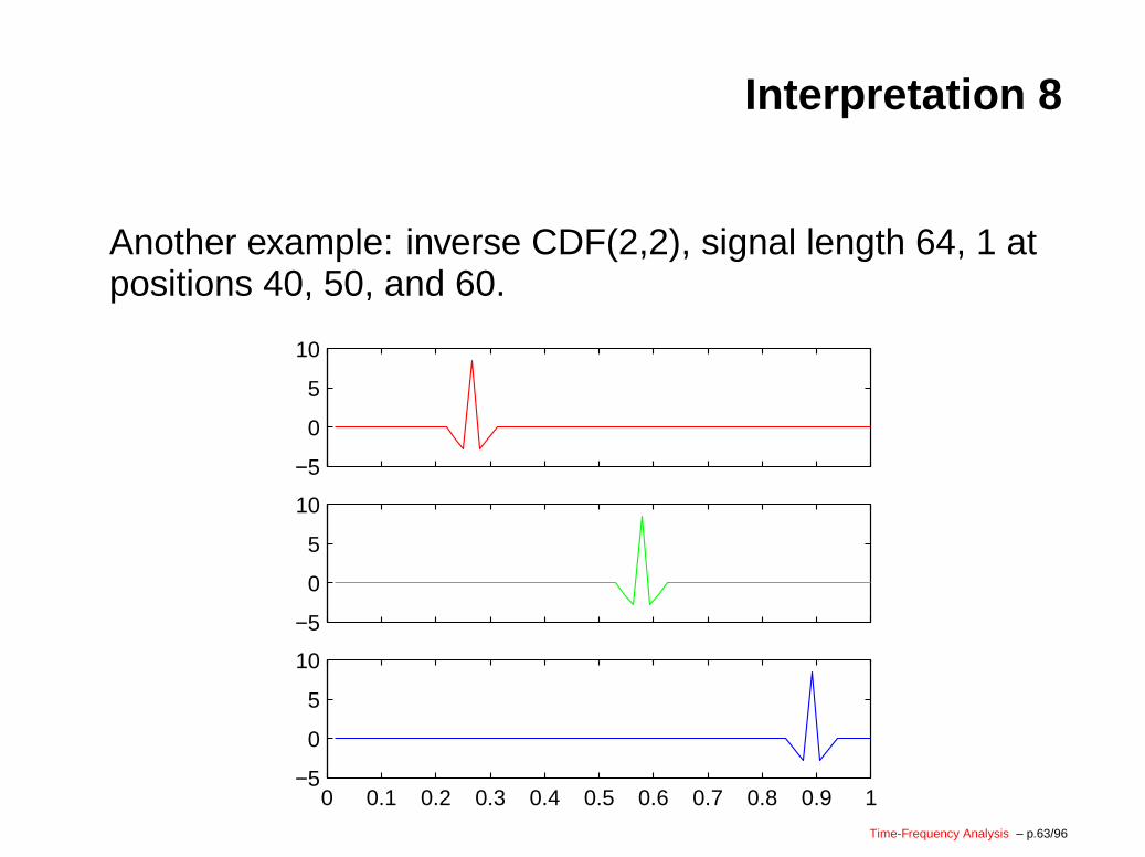
Interpretation 8
Another example: inverse CDF(2,2), signal length 64, 1 atpositions 40, 50, and 60.
−5
0
5
10
−5
0
5
10
0 0.1 0.2 0.3 0.4 0.5 0.6 0.7 0.8 0.9 1−5
0
5
10
Time-Frequency Analysis – p.63/96
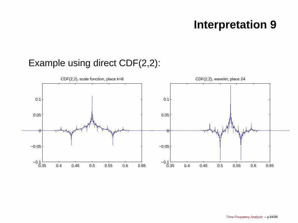
Interpretation 9
Example using direct CDF(2,2):
0.35 0.4 0.45 0.5 0.55 0.6 0.65−0.1
−0.05
0
0.05
0.1
CDF(2,2), scale function, place k=8
0.35 0.4 0.45 0.5 0.55 0.6 0.65−0.1
−0.05
0
0.05
0.1
CDF(2,2), wavelet, place 24
Time-Frequency Analysis – p.64/96
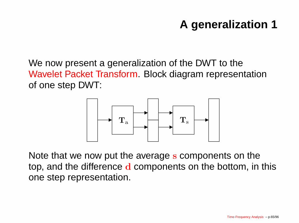
A generalization 1
We now present a generalization of the DWT to theWavelet Packet Transform. Block diagram representationof one step DWT:
TsTa
Note that we now put the average s components on thetop, and the difference d components on the bottom, in thisone step representation.
Time-Frequency Analysis – p.65/96
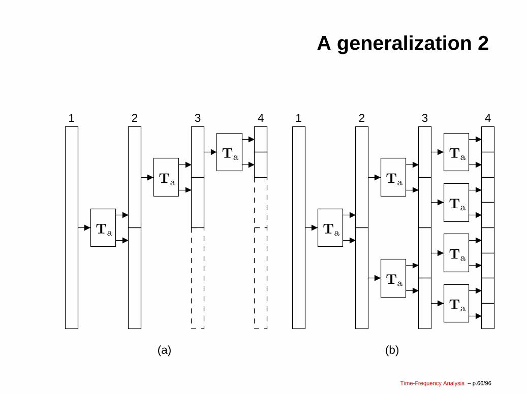
A generalization 2
1 2 3
Ta
Ta
Ta
Ta
Ta
Ta
Ta
1 2 3 4
Ta
Ta
Ta
4
(a) (b)
Time-Frequency Analysis – p.66/96
A generalization 3
Our first example, full decomposition:
Time-Frequency Analysis – p.67/96
A generalization 3
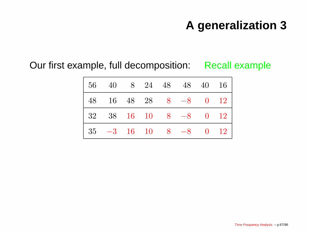
Our first example, full decomposition: Recall example
56 40 8 24 48 48 40 16
48 16 48 28 8 −8 0 12
32 38 16 10 8 −8 0 12
35 −3 16 10 8 −8 0 12
Time-Frequency Analysis – p.67/96
A generalization 3
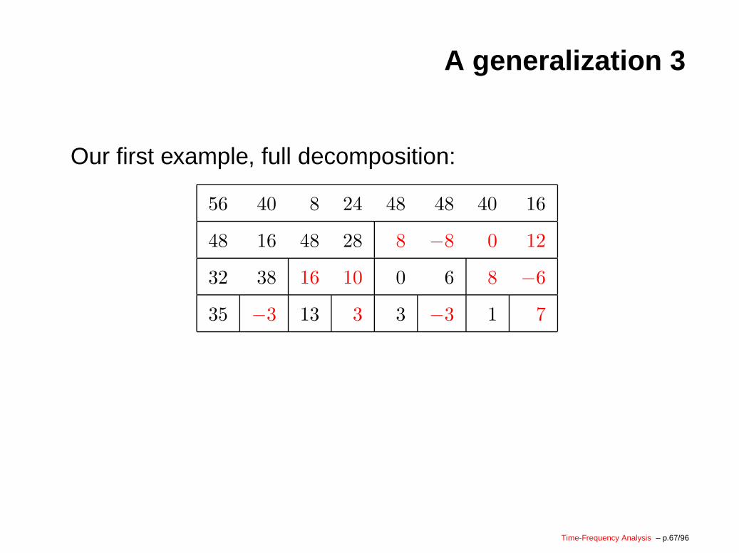
Our first example, full decomposition:
56 40 8 24 48 48 40 16
48 16 48 28 8 −8 0 12
32 38 16 10 0 6 8 −6
35 −3 13 3 3 −3 1 7
Time-Frequency Analysis – p.67/96
A generalization 3
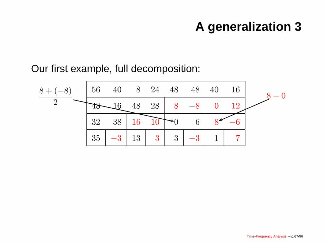
Our first example, full decomposition:
56 40 8 24 48 48 40 16
48 16 48 28 8 −8 0 12
32 38 16 10 0 6 8 −6
35 −3 13 3 3 −3 1 7
8 + (−8)
28− 0
Time-Frequency Analysis – p.67/96
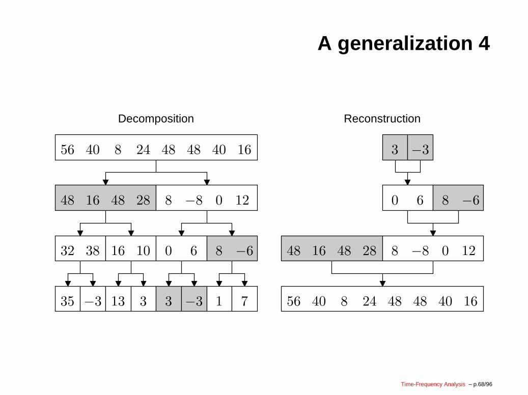
A generalization 4
56 40 8 24 48 48 40 16
−33
0 6 8 −6
Reconstruction
48 16 48 28 8 −8 0 12
40 8 24 48 48 40 16
48 16 48 28 8 −8 0
32 38 16 10 0 6 8 −6
1 7−33313−335
Decomposition
12
56
Time-Frequency Analysis – p.68/96
A generalization 5
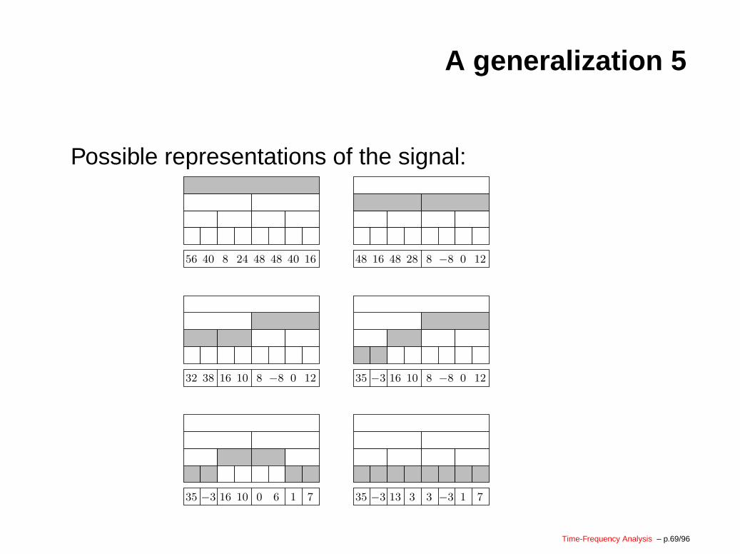
Possible representations of the signal:
56 40 8 24 48 48 40 16 48 16 48 28 8 −8 0 12
16 10 8 −8 0 1235 −3
35 −3 16 10 0 6 1 7 35 −3 1 713 3 3 −3
32 38 16 10 8 −8 0 12
Time-Frequency Analysis – p.69/96
WPT complexity 1
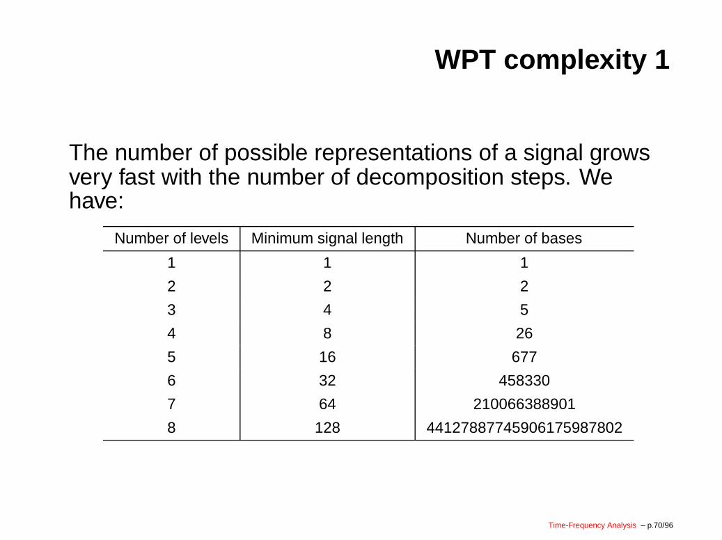
The number of possible representations of a signal growsvery fast with the number of decomposition steps. Wehave:
Number of levels Minimum signal length Number of bases
1 1 1
2 2 2
3 4 5
4 8 26
5 16 677
6 32 458330
7 64 210066388901
8 128 44127887745906175987802
Time-Frequency Analysis – p.70/96
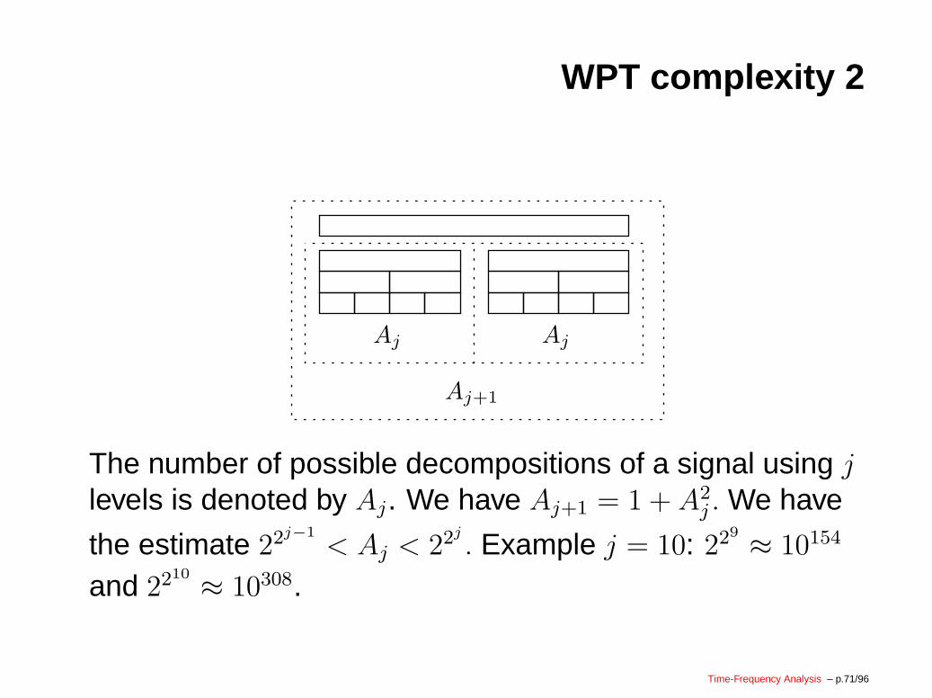
WPT complexity 2
AjAj
Aj+1
The number of possible decompositions of a signal using jlevels is denoted by Aj. We have Aj+1 = 1 + A2
j . We have
the estimate 22j−1
< Aj < 22j
. Example j = 10: 229 ≈ 10154
and 2210 ≈ 10308.
Time-Frequency Analysis – p.71/96
Best basis algorithm 1
Solution to complexity problem is the best basis algorithm.This is a very flexible algorithm, based on a cost function.A cost function is denoted by K. It maps a finite lengthsignal a to a number K(a). [ab] denotes the concatenationof two signals a and b. We require two properties:
K(0) = 0
K([ab]) = K(a) +K(b)
An example: K(a) = number of nonzero entries in a.
5 = K([1, 0, −1, 22, 0, 0, 2, −7]
= K([1, 0, −1, 22]) +K([0, 0, 2, −7]) = 3 + 2
Time-Frequency Analysis – p.72/96
Best basis algorithm 1
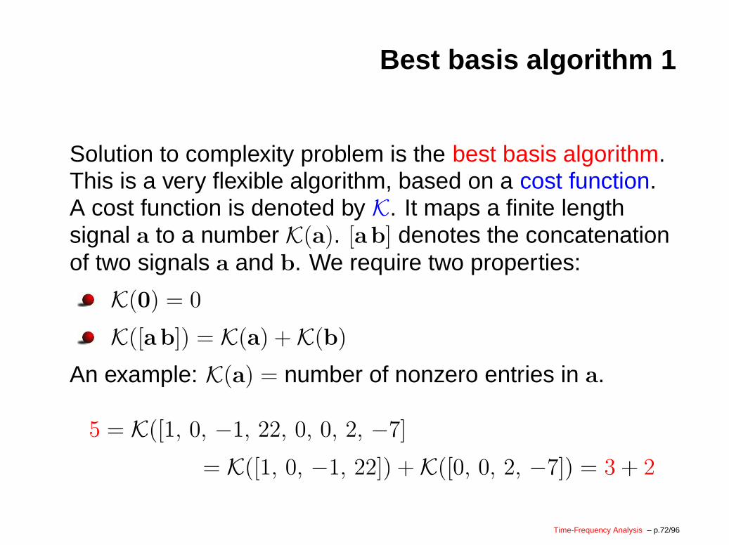
Solution to complexity problem is the best basis algorithm.This is a very flexible algorithm, based on a cost function.A cost function is denoted by K. It maps a finite lengthsignal a to a number K(a). [ab] denotes the concatenationof two signals a and b. We require two properties:
K(0) = 0
K([ab]) = K(a) +K(b)
An example: K(a) = number of nonzero entries in a.
5 = K([1, 0, −1, 22, 0, 0, 2, −7]
= K([1, 0, −1, 22]) +K([0, 0, 2, −7]) = 3 + 2
Time-Frequency Analysis – p.72/96
Best basis algorithm 2
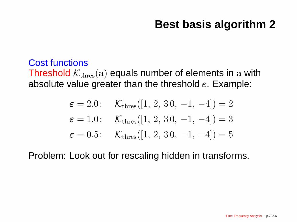
Cost functionsThreshold Kthres(a) equals number of elements in a withabsolute value greater than the threshold εεε. Example:
εεε = 2.0 : Kthres([1, 2, 3 0, −1, −4]) = 2
εεε = 1.0 : Kthres([1, 2, 3 0, −1, −4]) = 3
εεε = 0.5 : Kthres([1, 2, 3 0, −1, −4]) = 5
Problem: Look out for rescaling hidden in transforms.
Time-Frequency Analysis – p.73/96
Best basis algorithm 3
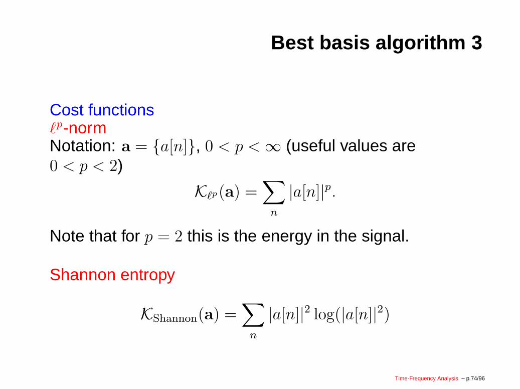
Cost functions`p-normNotation: a = {a[n]}, 0 < p <∞ (useful values are0 < p < 2)
K`p(a) =∑
n
|a[n]|p.
Note that for p = 2 this is the energy in the signal.
Shannon entropy
KShannon(a) =∑
n
|a[n]|2 log(|a[n]|2)
Time-Frequency Analysis – p.74/96
Best basis algorithm 4
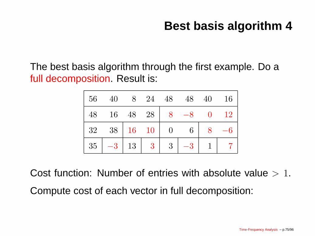
The best basis algorithm through the first example. Do afull decomposition. Result is:
56 40 8 24 48 48 40 16
48 16 48 28 8 −8 0 12
32 38 16 10 0 6 8 −6
35 −3 13 3 3 −3 1 7
Cost function: Number of entries with absolute value > 1.
Compute cost of each vector in full decomposition:
Time-Frequency Analysis – p.75/96
Best basis algorithm 5
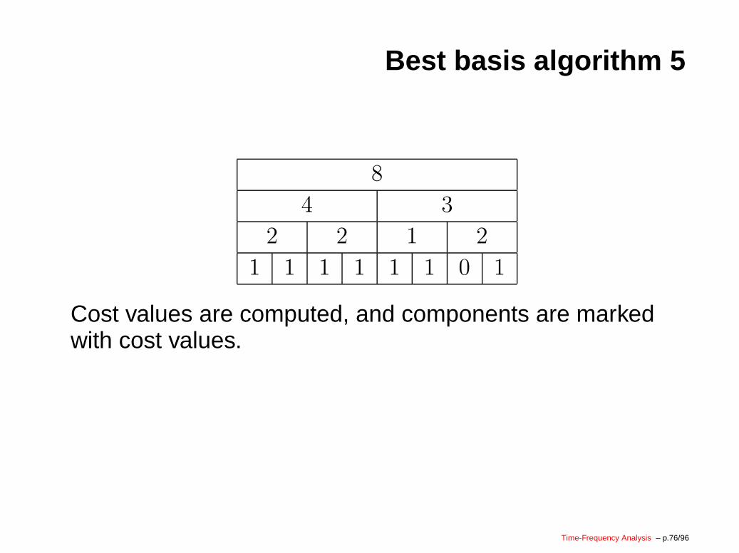
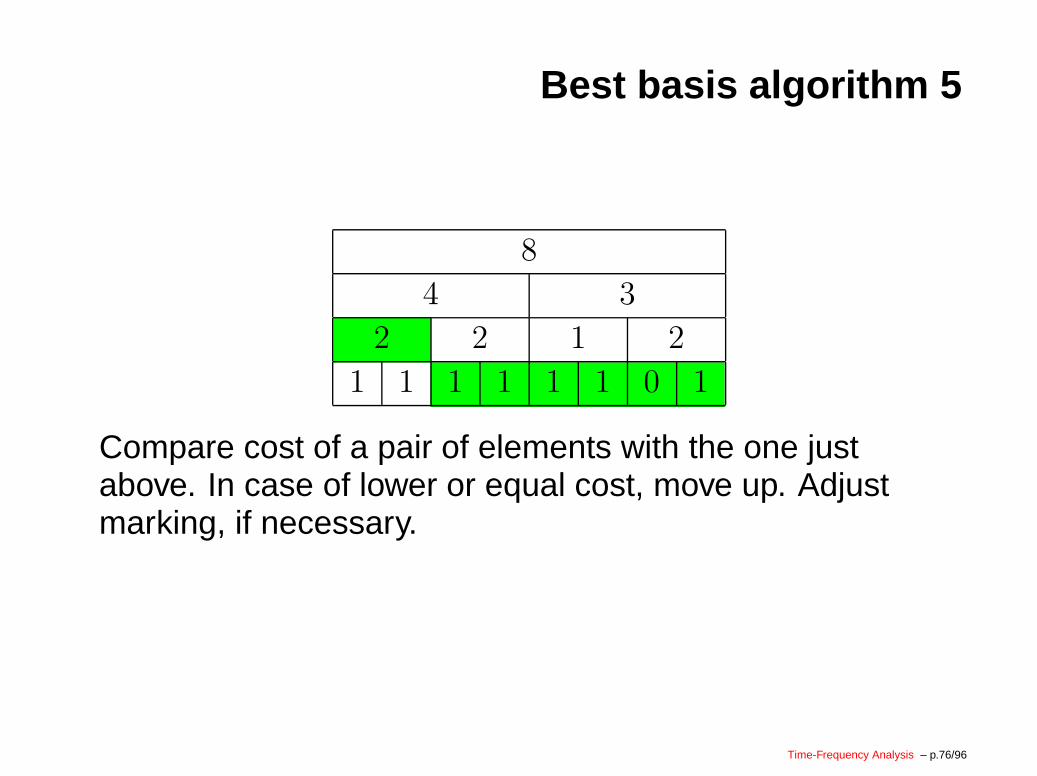
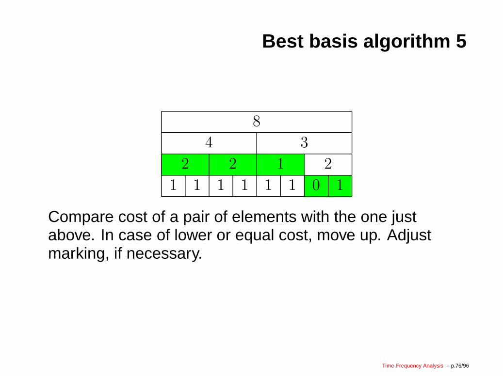
8
4 3
2 2 1 2
1 1 1 1 1 1 0 1
Cost values are computed, and components are markedwith cost values.
Time-Frequency Analysis – p.76/96
Best basis algorithm 5
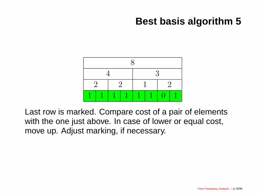
8
4 3
2 2 1 2
1 1 1 1 1 1 0 1
Last row is marked. Compare cost of a pair of elementswith the one just above. In case of lower or equal cost,move up. Adjust marking, if necessary.
Time-Frequency Analysis – p.76/96
Best basis algorithm 5
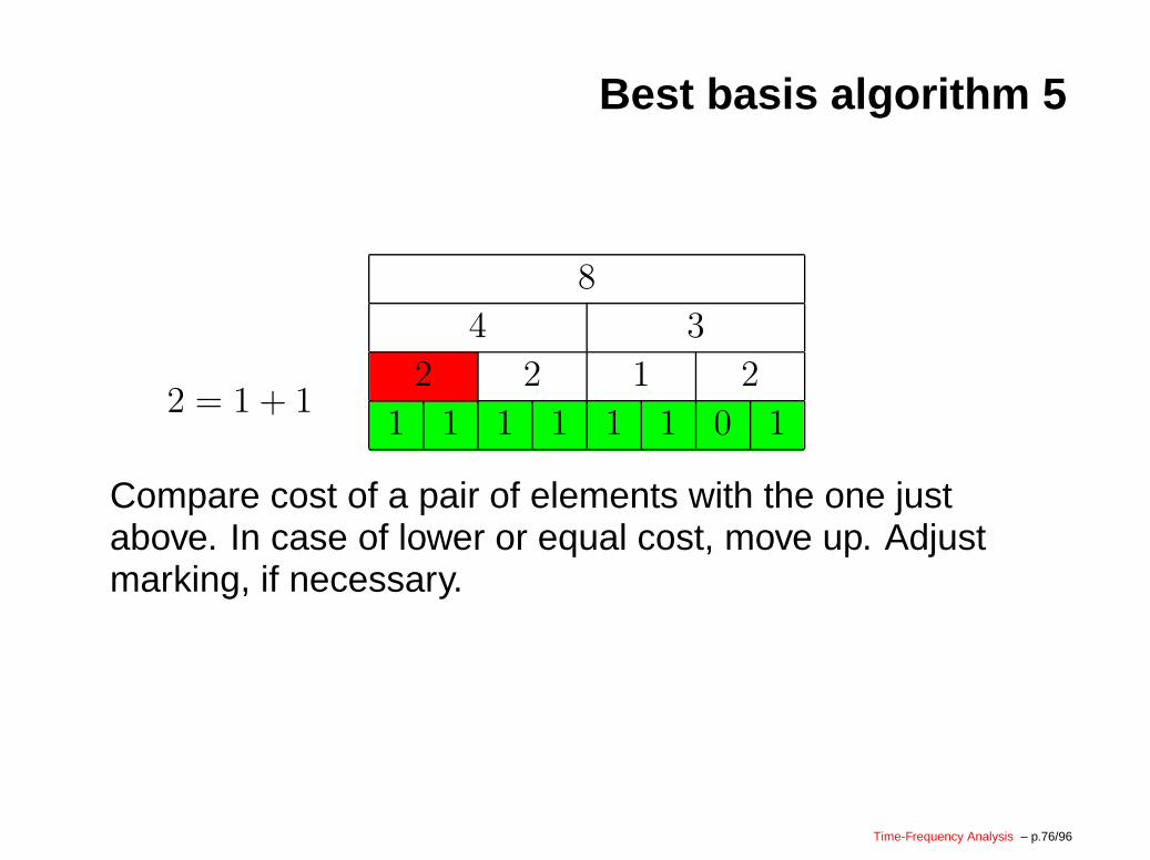
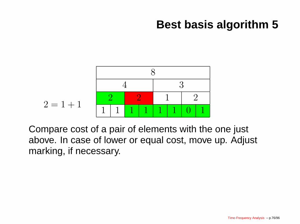
2 = 1 + 1
8
4 3
2 2 1 2
1 1 1 1 1 1 0 1
Compare cost of a pair of elements with the one justabove. In case of lower or equal cost, move up. Adjustmarking, if necessary.
Time-Frequency Analysis – p.76/96
Best basis algorithm 5
8
4 3
2 2 1 2
1 1 1 1 1 1 0 1
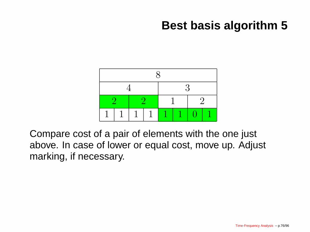
Compare cost of a pair of elements with the one justabove. In case of lower or equal cost, move up. Adjustmarking, if necessary.
Time-Frequency Analysis – p.76/96
Best basis algorithm 5
2 = 1 + 1
8
4 3
2 2 1 2
1 1 1 1 1 1 0 1
Compare cost of a pair of elements with the one justabove. In case of lower or equal cost, move up. Adjustmarking, if necessary.
Time-Frequency Analysis – p.76/96
Best basis algorithm 5
8
4 3
2 2 1 2
1 1 1 1 1 1 0 1
Compare cost of a pair of elements with the one justabove. In case of lower or equal cost, move up. Adjustmarking, if necessary.
Time-Frequency Analysis – p.76/96
Best basis algorithm 5
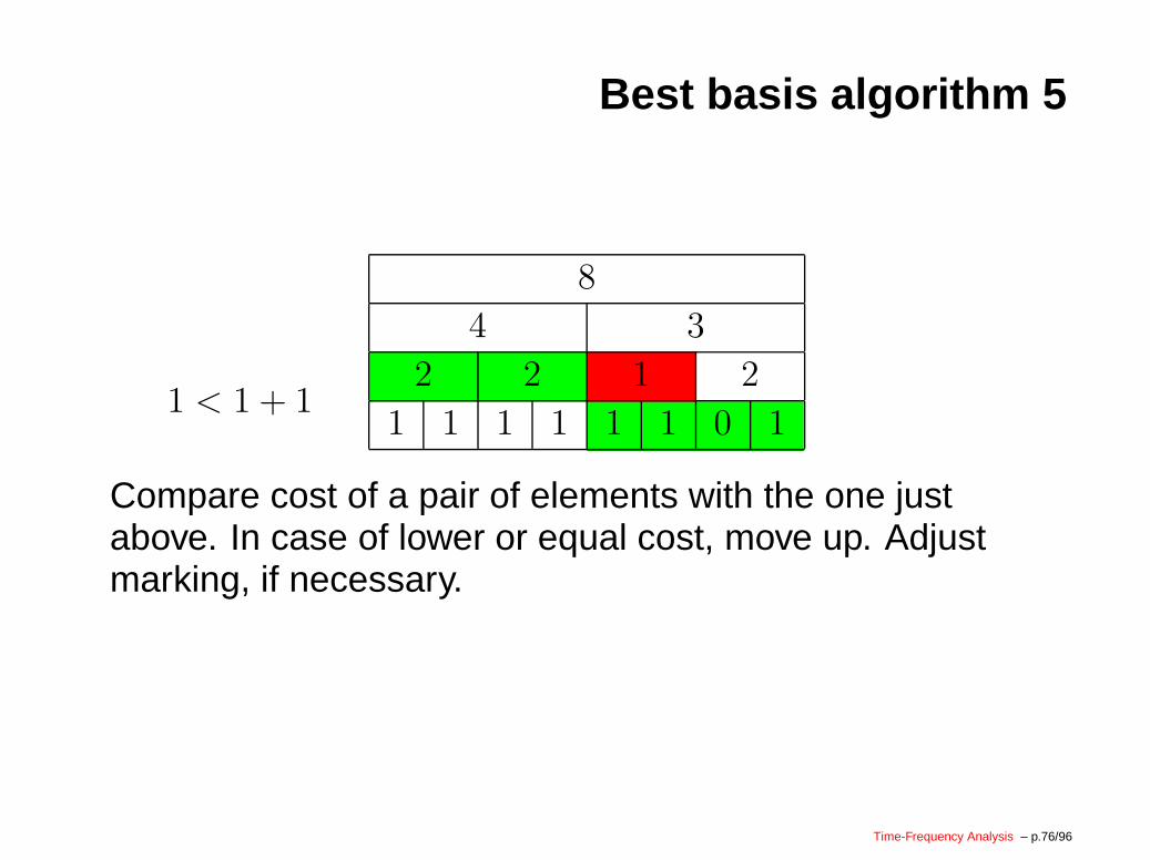
1 < 1 + 1
8
4 3
2 2 1 2
1 1 1 1 1 1 0 1
Compare cost of a pair of elements with the one justabove. In case of lower or equal cost, move up. Adjustmarking, if necessary.
Time-Frequency Analysis – p.76/96
Best basis algorithm 5
8
4 3
2 2 1 2
1 1 1 1 1 1 0 1
Compare cost of a pair of elements with the one justabove. In case of lower or equal cost, move up. Adjustmarking, if necessary.
Time-Frequency Analysis – p.76/96
Best basis algorithm 5
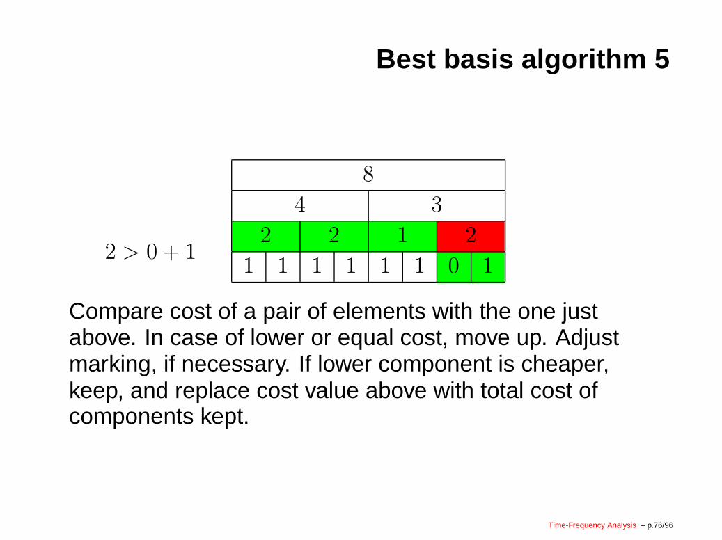
2 > 0 + 1
8
4 3
2 2 1 2
1 1 1 1 1 1 0 1
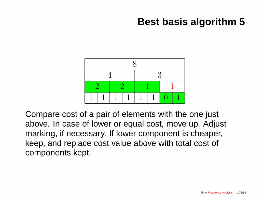
Compare cost of a pair of elements with the one justabove. In case of lower or equal cost, move up. Adjustmarking, if necessary. If lower component is cheaper,keep, and replace cost value above with total cost ofcomponents kept.
Time-Frequency Analysis – p.76/96
Best basis algorithm 5
8
4 3
2 2 1 1
1 1 1 1 1 1 0 1
Compare cost of a pair of elements with the one justabove. In case of lower or equal cost, move up. Adjustmarking, if necessary. If lower component is cheaper,keep, and replace cost value above with total cost ofcomponents kept.
Time-Frequency Analysis – p.76/96
Best basis algorithm 5
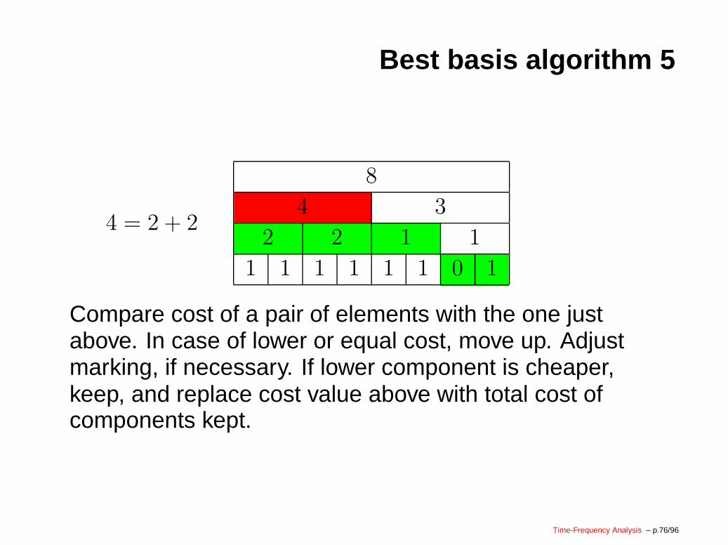
4 = 2 + 2
8
4 3
2 2 1 1
1 1 1 1 1 1 0 1
Compare cost of a pair of elements with the one justabove. In case of lower or equal cost, move up. Adjustmarking, if necessary. If lower component is cheaper,keep, and replace cost value above with total cost ofcomponents kept.
Time-Frequency Analysis – p.76/96

Best basis algorithm 5
8
4 3
2 2 1 1
1 1 1 1 1 1 0 1
Compare cost of a pair of elements with the one justabove. In case of lower or equal cost, move up. Adjustmarking, if necessary. If lower component is cheaper,keep, and replace cost value above with total cost ofcomponents kept.
Time-Frequency Analysis – p.76/96
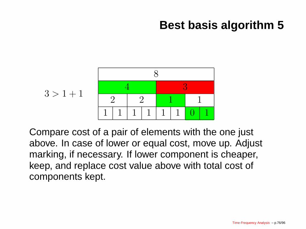
Best basis algorithm 5
3 > 1 + 1
8
4 3
2 2 1 1
1 1 1 1 1 1 0 1
Compare cost of a pair of elements with the one justabove. In case of lower or equal cost, move up. Adjustmarking, if necessary. If lower component is cheaper,keep, and replace cost value above with total cost ofcomponents kept.
Time-Frequency Analysis – p.76/96
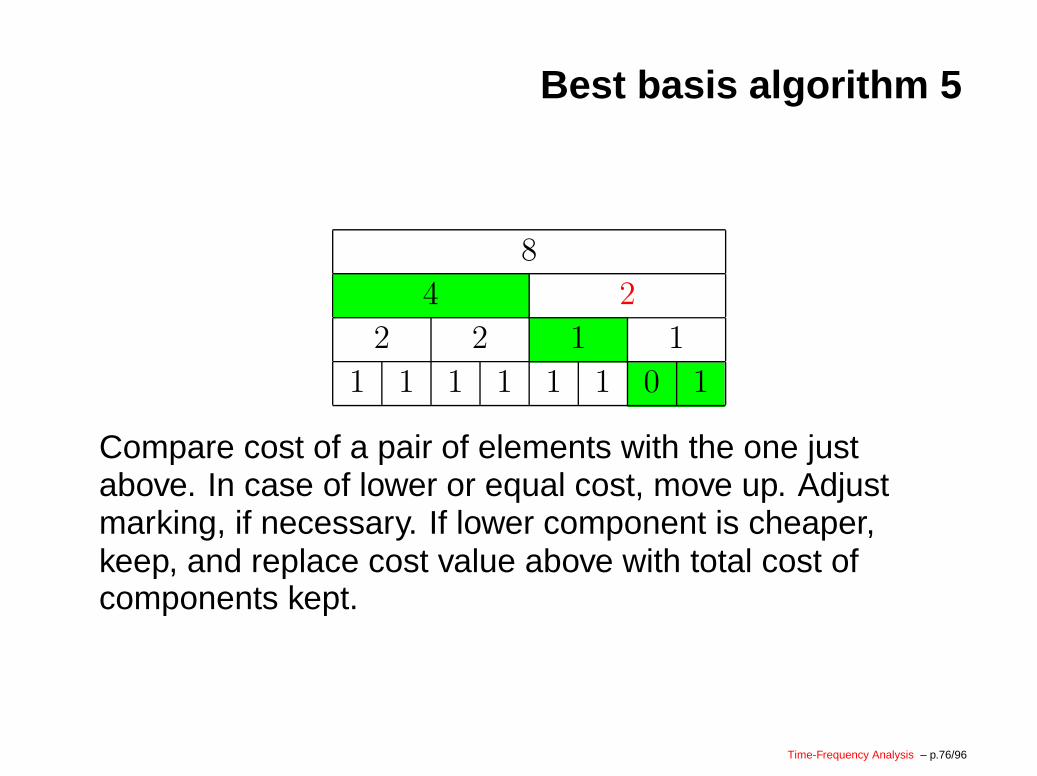
Best basis algorithm 5
8
4 2
2 2 1 1
1 1 1 1 1 1 0 1
Compare cost of a pair of elements with the one justabove. In case of lower or equal cost, move up. Adjustmarking, if necessary. If lower component is cheaper,keep, and replace cost value above with total cost ofcomponents kept.
Time-Frequency Analysis – p.76/96
Best basis algorithm 5
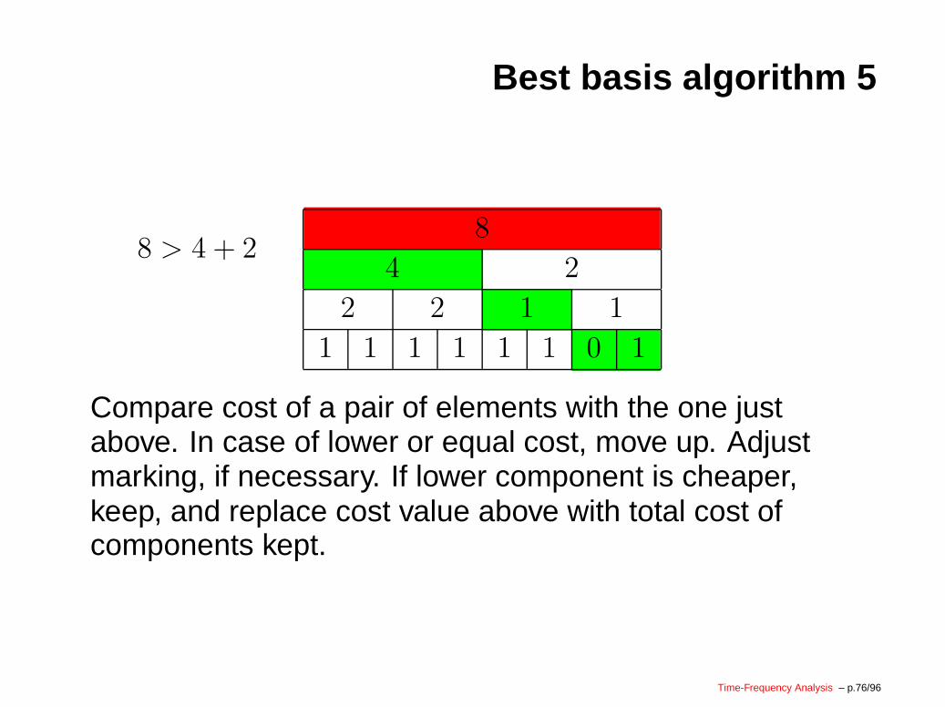
8 > 4 + 28
4 2
2 2 1 1
1 1 1 1 1 1 0 1
Compare cost of a pair of elements with the one justabove. In case of lower or equal cost, move up. Adjustmarking, if necessary. If lower component is cheaper,keep, and replace cost value above with total cost ofcomponents kept.
Time-Frequency Analysis – p.76/96

Best basis algorithm 5
6
4 2
2 2 1 1
1 1 1 1 1 1 0 1
Compare cost of a pair of elements with the one justabove. In case of lower or equal cost, move up. Adjustmarking, if necessary. If lower component is cheaper,keep, and replace cost value above with total cost ofcomponents kept.
Time-Frequency Analysis – p.76/96
Best basis algorithm 6
Some things to note:
The best basis is not unique.
A best basis with all components at the same level iscalled a best level basis.
With J levels the search algorithm is of orderO(J log J). The full decomposition and the costs haveto be computed only once.
The size of the tree to be searched is independent ofthe length of the signal.
Time-Frequency Analysis – p.77/96
Time and frequency 1
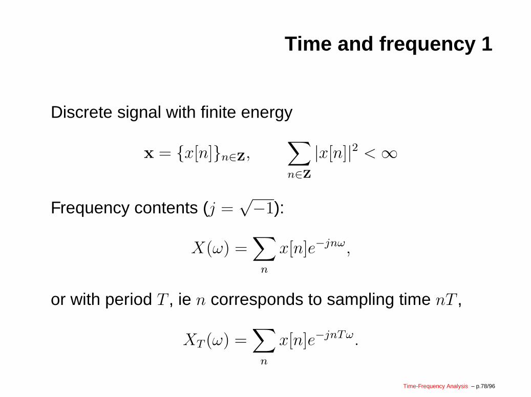
Discrete signal with finite energy
x = {x[n]}n∈Z,∑
n∈Z
|x[n]|2 <∞
Frequency contents (j =√−1):
X(ω) =∑
n
x[n]e−jnω,
or with period T , ie n corresponds to sampling time nT ,
XT (ω) =∑
n
x[n]e−jnTω.
Time-Frequency Analysis – p.78/96
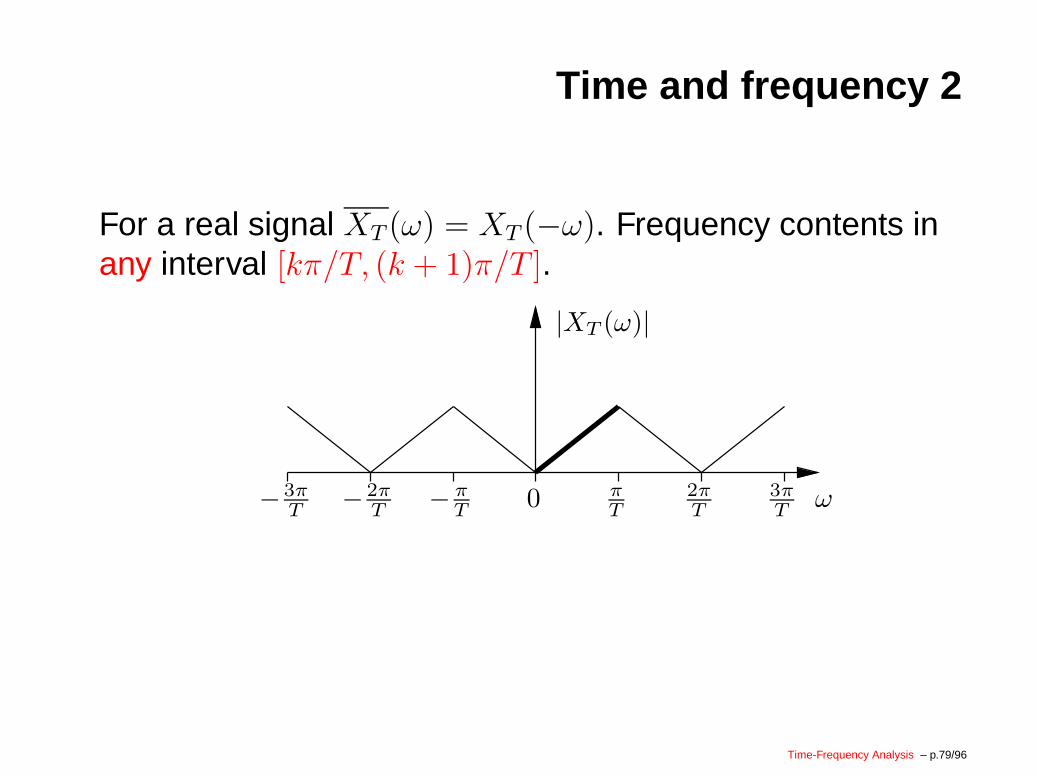
Time and frequency 2
For a real signal XT (ω) = XT (−ω). Frequency contents inany interval [kπ/T, (k + 1)π/T ].
0
|XT (ω)|
ω− πT
− 3πT
3πT
πT
− 2πT
2πT
Time-Frequency Analysis – p.79/96
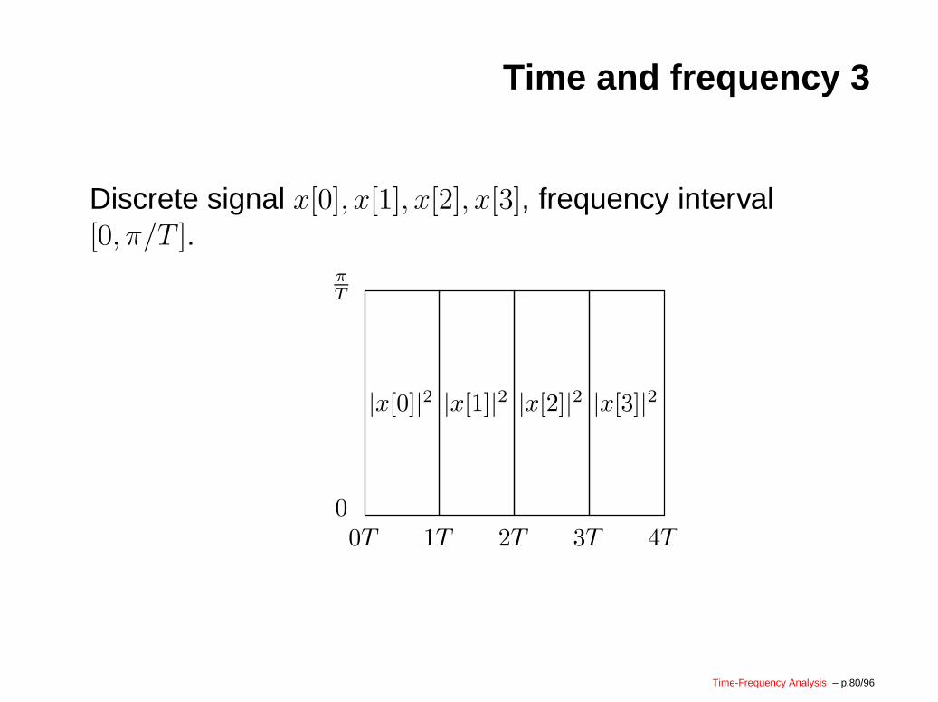
Time and frequency 3
Discrete signal x[0], x[1], x[2], x[3], frequency interval[0, π/T ].
|x[0]|2 |x[1]|2 |x[2]|2 |x[3]|2
0T 1T 2T 4T
πT
3T0
Time-Frequency Analysis – p.80/96
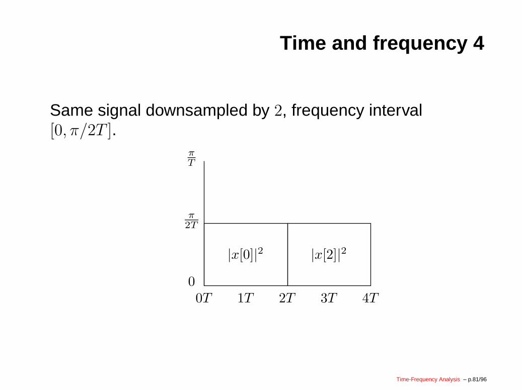
Time and frequency 4
Same signal downsampled by 2, frequency interval[0, π/2T ].
|x[2]|2|x[0]|2
0T 1T 2T 4T
πT
3T0
π2T
Time-Frequency Analysis – p.81/96
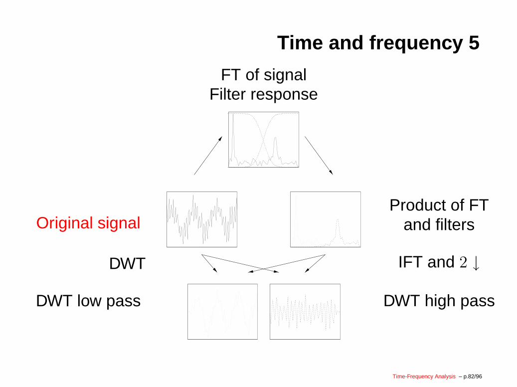
Time and frequency 5
Original signal
FT of signalFilter response
Product of FTand filters
DWT low pass DWT high pass
DWT IFT and 2 ↓
Time-Frequency Analysis – p.82/96
Time and frequency 6
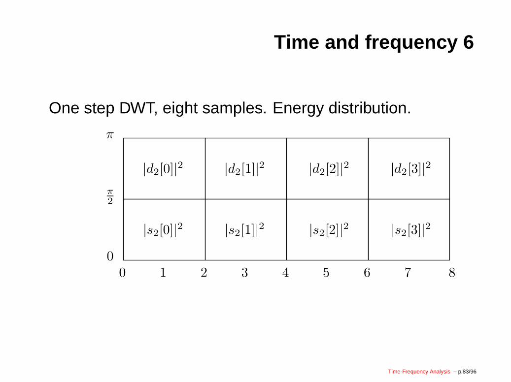
One step DWT, eight samples. Energy distribution.
|s2[1]|2|s2[0]|2 |s2[2]|2 |s2[3]|2
|d2[0]|2 |d2[1]|2 |d2[2]|2 |d2[3]|2
0 1 4
π
30
π2
6 7 852
Time-Frequency Analysis – p.83/96
Time and frequency 7
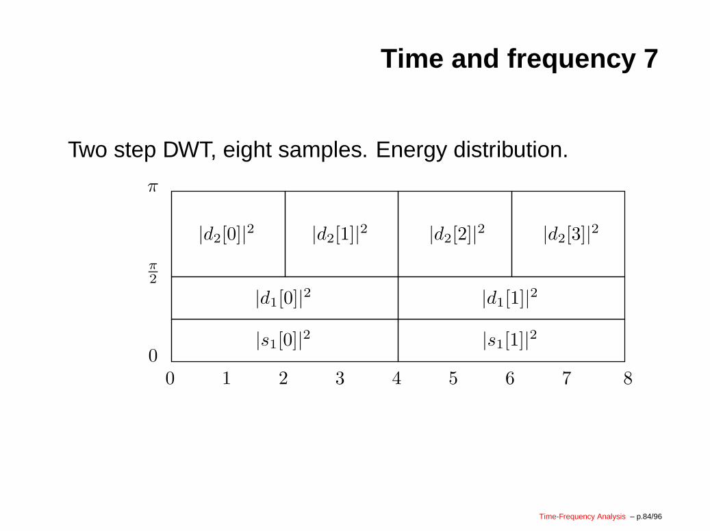
Two step DWT, eight samples. Energy distribution.
|d2[0]|2 |d2[1]|2 |d2[2]|2 |d2[3]|2
|s1[0]|2 |s1[1]|2|d1[1]|2|d1[0]|2
0 1 4
π
30
π2
6 7 852
Time-Frequency Analysis – p.84/96
Time and frequency 8
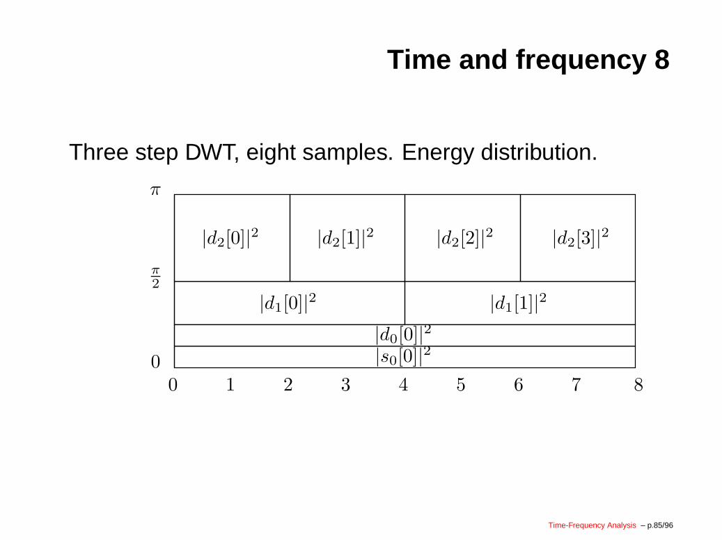
Three step DWT, eight samples. Energy distribution.
|d2[0]|2 |d2[1]|2 |d2[2]|2 |d2[3]|2
|d1[1]|2|d1[0]|2
0 1 4
π
30
π2
6 7 852
|s0[0]|2|d0[0]|2
Time-Frequency Analysis – p.85/96
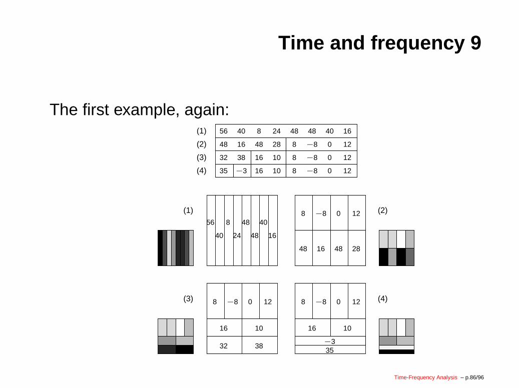
Time and frequency 9
The first example, again:
(1) (2)
(3) (4)
56
40
8
24
48
48
40
16
−8 0 128
3832−335
35 −3
32 38
28481648
56 40 8 24 16404848(1)
(2)
(4)
(3)
48 16 48 28
−8 0 128
10161016
−8 0 128
0
016 10
8 0 12
16 10
−8
−8
8
−8
8
12
12
Time-Frequency Analysis – p.86/96
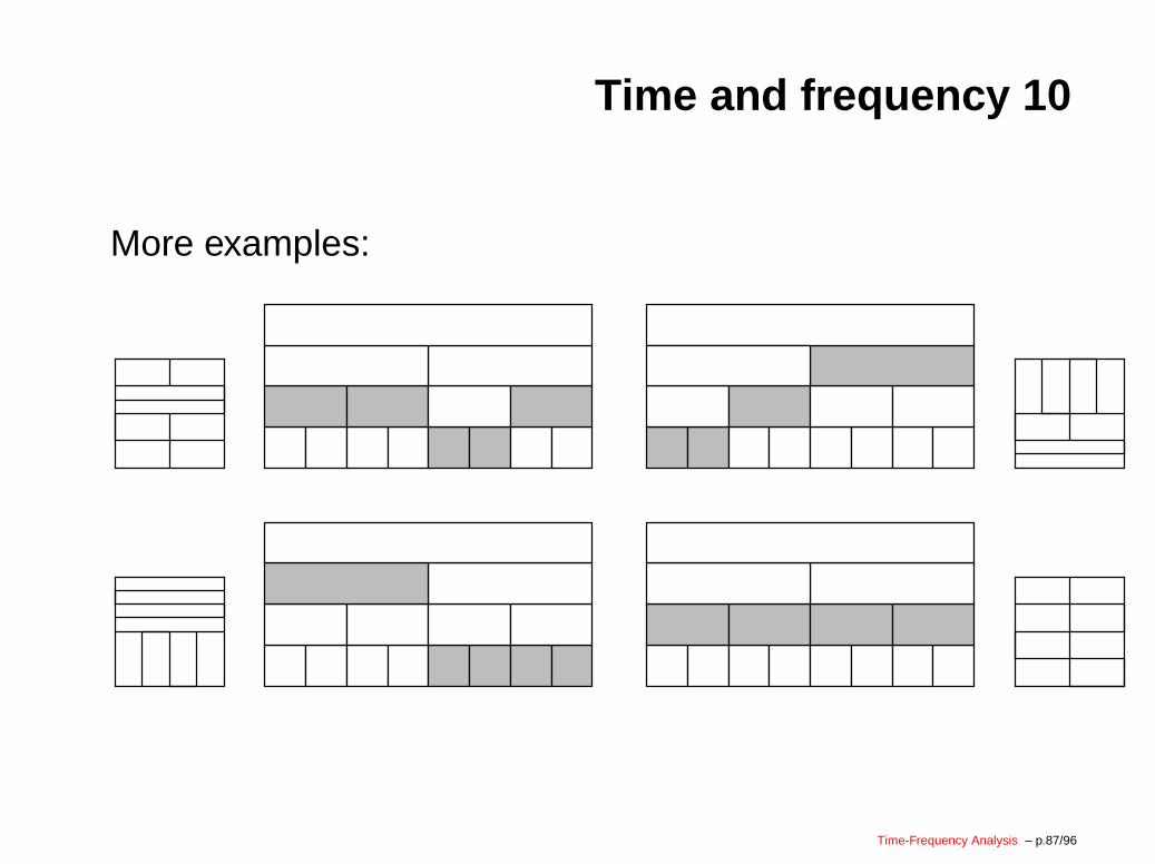
Time and frequency 10
More examples:
Time-Frequency Analysis – p.87/96
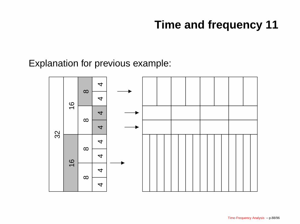
Time and frequency 11
Explanation for previous example:
44
44
44
44
88
88
1616
32
Time-Frequency Analysis – p.88/96
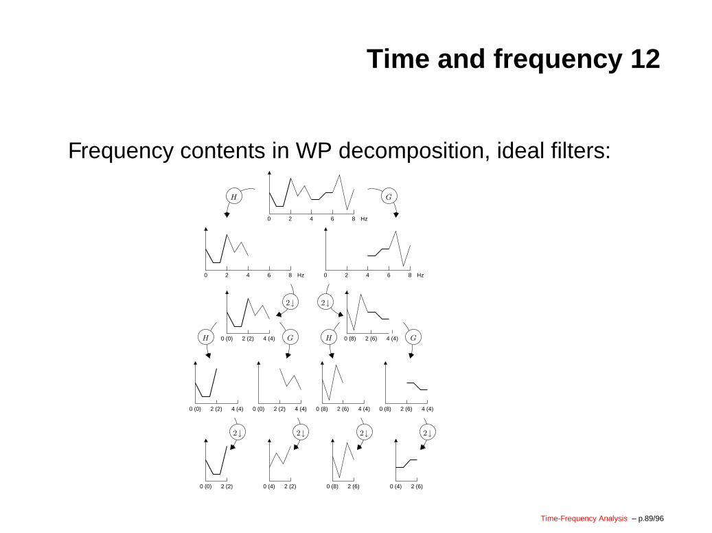
Time and frequency 12
Frequency contents in WP decomposition, ideal filters:
2↓2↓ 2↓2↓
G
2↓
H G
H
H G
2↓
0 (0) 2 (2) 4 (4)
0 (0)
2 (2)
0 (4)
0 (0) 4 (4) 2 (6) 4 (4)0 (8)
0 (8) 2 (6)
4 (4)0 (8)
0 (4) 2 (6)2 (2)2 (2)
2 (6)
4 (4)2 (2)0 (0)
0 2 4 6 8 Hz
0 2 4 6 8 Hz
Hz86420
4 (4)2 (6)0 (8)
Time-Frequency Analysis – p.89/96
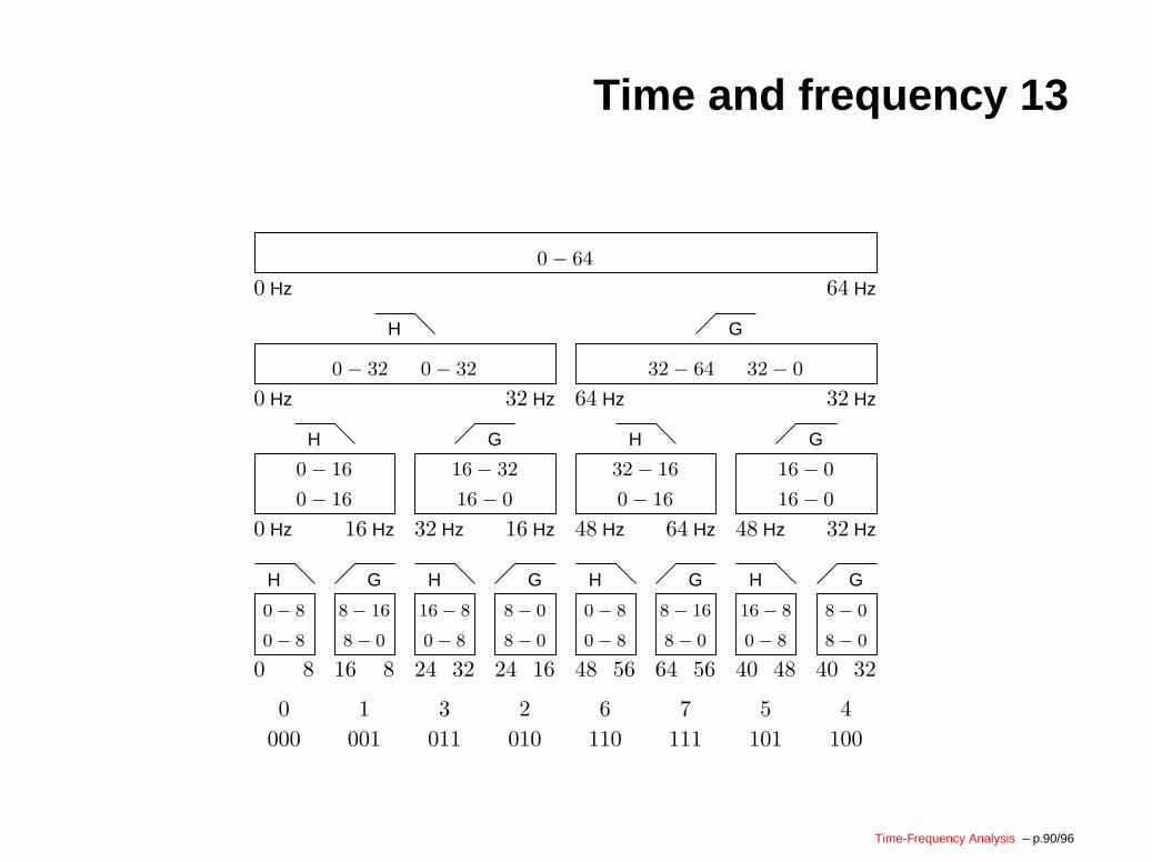
Time and frequency 13
H G H G H G H G
H G H G
GH
0
000
1
001
3
011
2
010
6
110
7
111
5
101
4
100
0− 16
0− 16 16− 0
16− 32
0− 16
32− 16
16− 0
16 Hz0 Hz 32 Hz 16 Hz 48 Hz 64 Hz 48 Hz 32 Hz
0 − 8
0 − 8 8 − 16
8 − 0
16 − 8
0 − 8
8 − 0
8 − 0
0 − 8
0 − 8
8 − 16
8 − 0
16 − 8
0 − 8
8 − 0
8 − 0
0 8 16 8 24 32 24 16 48 56 64 56 40 48 40 32
0− 32 0− 32 32− 64 32− 0
0 Hz 32 Hz 64 Hz 32 Hz
0− 64
64 Hz0 Hz
16− 0
Time-Frequency Analysis – p.90/96
Time and frequency 14
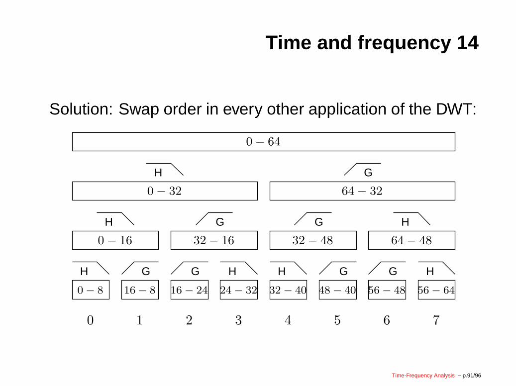
Solution: Swap order in every other application of the DWT:
H
0 − 8 16 − 8 16 − 24 24 − 32 32 − 40 48 − 40 56 − 48 56 − 64
G G H H G G H
GH G H
G
32− 160− 16 32− 48 64− 48
0− 32 64− 32
0− 64
0 1 2 3 4 5 6 7
H
Time-Frequency Analysis – p.91/96
Time and frequency 15
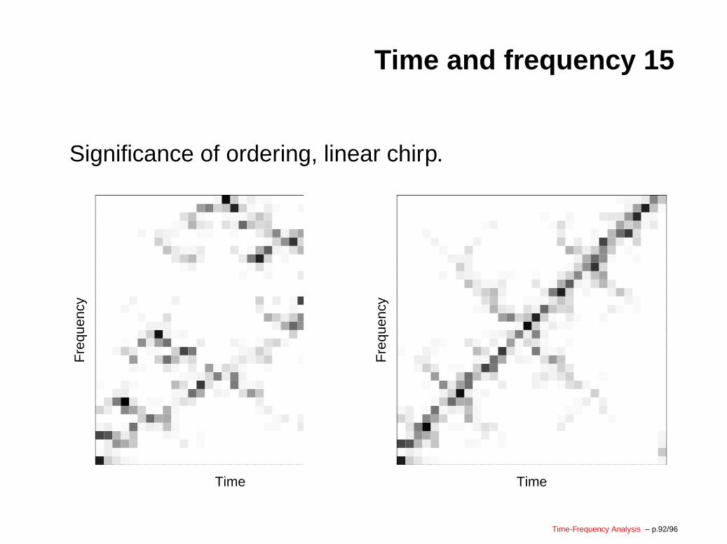
Significance of ordering, linear chirp.
Time
Fre
quen
cy
Time
Fre
quen
cy
Time-Frequency Analysis – p.92/96
Time and frequency 16
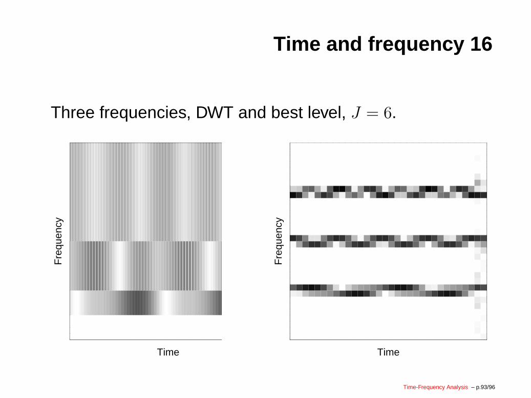
Three frequencies, DWT and best level, J = 6.
Time
Fre
quen
cy
Time
Fre
quen
cy
Time-Frequency Analysis – p.93/96
Time and frequency 17
A complicated signal, length 1024: Sum of
x[n] =
25 if n = 300 ,
1 if 500 ≤ n ≤ 700 ,
15 if n = 900 ,
0 otherwise .
andsin(ω0t) + sin(2ω0t) + sin(3ω0t) ,
with ω0 = 405.5419.
Time-Frequency Analysis – p.94/96
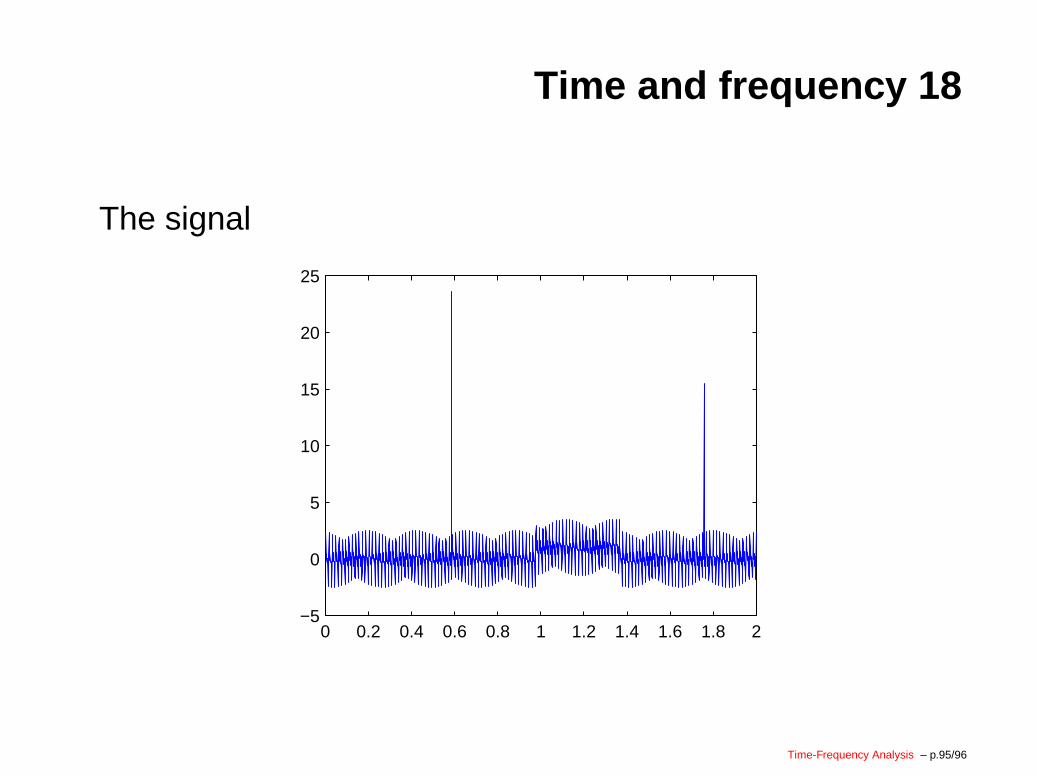
Time and frequency 18
The signal
0 0.2 0.4 0.6 0.8 1 1.2 1.4 1.6 1.8 2−5
0
5
10
15
20
25
Time-Frequency Analysis – p.95/96
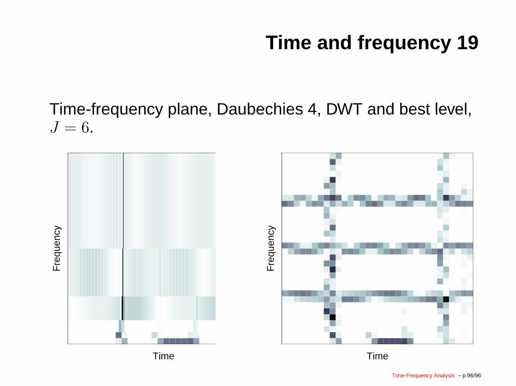
Time and frequency 19
Time-frequency plane, Daubechies 4, DWT and best level,J = 6.
Time
Fre
quen
cy
Time
Fre
quen
cy
Time-Frequency Analysis – p.96/96