Embed Size (px)
Citation preview

Introduction Macroeconomic Dynamics Asset Pricing Implications
Time-varying Risk of NominalBonds: How Important Are
Macroeconomic Shocks?
Andrey Ermolov
Columbia Business School
February 9, 2015
1 / 45
Introduction Macroeconomic Dynamics Asset Pricing Implications
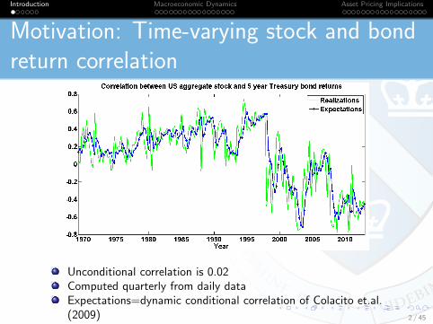
Motivation: Time-varying stock and bondreturn correlation
Unconditional correlation is 0.02Computed quarterly from daily dataExpectations=dynamic conditional correlation of Colacito et.al.(2009) 2 / 45
Introduction Macroeconomic Dynamics Asset Pricing Implications
Stock and bond return correlation -important but difficult to explain moment
Important:First order effect on portfolio variance
Stocks and bonds large and closely integratedmarkets: should be modeled jointly
Difficult to explain:Theoretically: starting from Shiller and Beltratti(1992)
Empirically: e.g., even in dynamic factor models(Baele et.al., 2010)
3 / 45
Introduction Macroeconomic Dynamics Asset Pricing Implications
Question
Are macroeconomic shocks (consumptiongrowth and inflation) related to time-varyingstock and bond return correlation?
Can they generate correlations of observedmagnitudes?
Historically, how much do they matter at differentpoints in time?
4 / 45
Introduction Macroeconomic Dynamics Asset Pricing Implications
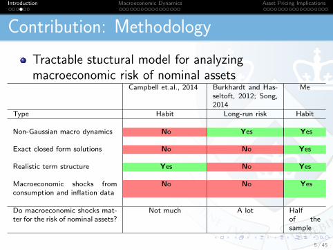
Contribution: Methodology
Tractable stuctural model for analyzingmacroeconomic risk of nominal assets
Campbell et.al., 2014 Burkhardt and Has-seltoft, 2012; Song,2014
Me
Type Habit Long-run risk Habit
Non-Gaussian macro dynamics No Yes Yes
Exact closed form solutions No No Yes
Realistic term structure Yes No Yes
Macroeconomic shocks fromconsumption and inflation data
No No Yes
Do macroeconomic shocks mat-ter for the risk of nominal assets?
Not much A lot Halfof thesample
5 / 45
Introduction Macroeconomic Dynamics Asset Pricing Implications
Contribution: Empirical results
Economically intuitive characterization ofmacroeconomic shocks
Implications for stock and bond return correlation:
macroeconomic shocks generate sizeable positiveand negative correlations, although negativecorrelations smaller and less frequent than in data
historically, macroeconomic shocks are importantin explaining high correlations from late 70’s toearly 90’s and low correlations pre- and during theGreat Recession
6 / 45

Introduction Macroeconomic Dynamics Asset Pricing Implications
Overview of the model
External habit utility:
realistic asset pricing moments: in particular,realistic term structure
Macroeconomic dynamics from Bekaert,Engstrom, and Ermolov (2014c):
convenient for modeling time-varying bond risk:drives time-varying stock and bond returncorrelations
7 / 45
Introduction Macroeconomic Dynamics Asset Pricing Implications
Consumption growth and inflation
Consumption growth: gt+1 = g + εgt+1
Constant mean g
Heteroskedastic 0-mean shock εgt+1
Inflation: πt+1 = π + xπt + επt+1
Unconditional mean π
Persistent 0-mean inflation expectations xπt
Heteroskedastic 0-mean shock επt+1
8 / 45
Introduction Macroeconomic Dynamics Asset Pricing Implications
Macroeconomic shocks
εgt+1 = σdg︸︷︷︸>0
udt+1 + σsg︸︷︷︸>0
ust+1,
επt+1 = σdπ︸︷︷︸>0
udt+1 − σsπ︸︷︷︸>0
ust+1,
Cov(udt+1, ust+1) = 0,Var(udt+1) = Var(ust+1) = 1.
udt+1 - ”demand shock”: moves gt+1 and πt+1 in the
same direction ⇒ nominal bonds hedge well
ust+1 - ”supply shock”: moves gt+1 and πt+1 in opposite
directions ⇒ nominal bonds hedge poorly
udt+1 and us
t+1 heteroskedastic, butVar(ud
t+1) = Var(ust+1) = 1, Cov(ud
t+1, ust+1) = 0
9 / 45
Introduction Macroeconomic Dynamics Asset Pricing Implications
Macroeconomic environments
If supply and demand shocks are heteroskedastic,Covt(ε
gt+1, ε
πt+1) will vary over time:
Covt(εgt+1, ε
πt+1) = σd
gσdπVart(u
dt+1)− σs
gσsπVart(u
st+1)
Demand shock environment: Covt(εgt+1, ε
πt+1) > 0 ⇒
nominal bonds hedge well
Supply shock environment: Covt(εgt+1, ε
πt+1) < 0 ⇒
nominal bonds hedge poorly
10 / 45

Introduction Macroeconomic Dynamics Asset Pricing Implications
Modeling demand and supply shocks
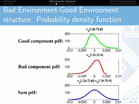
Demand and supply shocks modeled using BadEnvironment-Good Environment (BEGE) structure(Bekaert and Engstrom, 2014): component models oftwo 0-mean shocks
udt+1 = σd
pωdp,t+1 − σd
nωdn,t+1,
ust+1 = σs
pωsp,t+1 − σs
nωsn,t+1,
}ωp,t+1 - good shockωn,t+1 - bad shock
Shocks follow demeaned gamma distributions:
ωdp,t+1 ∼ Γ(pdt , 1)− pdt ,
ωdn,t+1 ∼ Γ(ndt , 1)− ndt ,
ωsp,t+1 ∼ Γ(pst , 1)− pst ,
ωsn,t+1 ∼ Γ(nst , 1)− nst .
Γ(x , y)−gamma distribution withshape parameter x andscale parameter y
11 / 45
Introduction Macroeconomic Dynamics Asset Pricing Implications
Bad Environment-Good Environmentstructure: Probability density function
12 / 45
Introduction Macroeconomic Dynamics Asset Pricing Implications
Time-varying variances
pt can be interpreted as good variance and ntas bad variance
Variances are persistent and driven by therealization shocks, capturing volatilityclustering (Gourieroux and Jasiak, 2006):
pdt+1 = pd + ρdp(pdt − pd) + σdppωdp,t+1,
Similar processes for ndt+1, pst+1, nst+1
13 / 45
Introduction Macroeconomic Dynamics Asset Pricing Implications
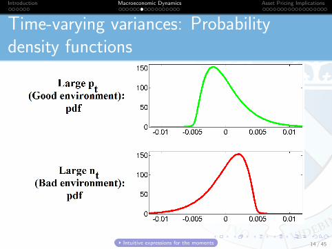
Time-varying variances: Probabilitydensity functions
Intuitive expressions for the moments 14 / 45
Introduction Macroeconomic Dynamics Asset Pricing Implications
Model: Why gamma distributed shocks?
Empirically supported to capture non-Gaussian featuresprevalent in consumption and inflation data (Bekaertand Engstrom, 2014; Bekaert, Engstrom, and Ermolov,2014a,b)
Non-Gaussian features facilitate theoretically matchingrisk-premia
Intuitive closed form solutions
Efficient estimation
15 / 45

Introduction Macroeconomic Dynamics Asset Pricing Implications
Data
US quarterly observations: 1969Q4-2012Q4
Working (1960) adjusted consumption ofnon-durables and services
Inflation: St.Louis Fed
Inflation expectations: Survey of ProfessionalForecasters
16 / 45
Introduction Macroeconomic Dynamics Asset Pricing Implications
Estimation
Maximum likelihood estimation using onlymacroeconomic data (no financial data)
Input: consumption growth and inflation time series
Output 1: macroeconomic dynamics parametersestimates
Output 2: expected pdt , ndt , pst , nst time series
Methodology: sequentially computing likelihood overobservations - in characteristic function domain formulasfor computing likelihood available in closed form (Bates,2006)
Detailed estimation overview Maximum likelihood estimation overview
17 / 45
Introduction Macroeconomic Dynamics Asset Pricing Implications
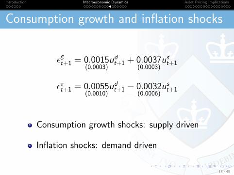
Consumption growth and inflation shocks
εgt+1 = 0.0015(0.0003)
udt+1 + 0.0037(0.0003)
ust+1
επt+1 = 0.0055(0.0010)
udt+1 − 0.0032(0.0006)
ust+1
Consumption growth shocks: supply driven
Inflation shocks: demand driven
18 / 45
Introduction Macroeconomic Dynamics Asset Pricing Implications
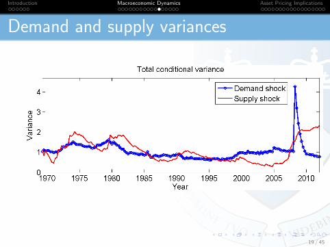
Demand and supply variances
19 / 45
Introduction Macroeconomic Dynamics Asset Pricing Implications
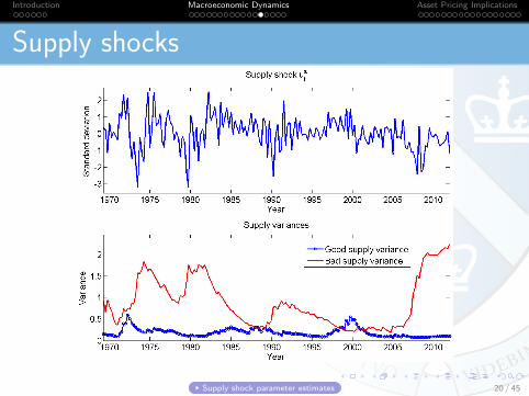
Supply shocks
Supply shock parameter estimates 20 / 45
Introduction Macroeconomic Dynamics Asset Pricing Implications
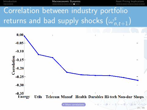
Correlation between industry portfolioreturns and bad supply shocks (ωs
n,t+1)
More correlations
21 / 45
Introduction Macroeconomic Dynamics Asset Pricing Implications
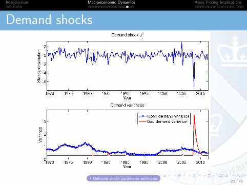
Demand shocks
Demand shock parameter estimates22 / 45
Introduction Macroeconomic Dynamics Asset Pricing Implications
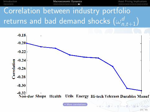
Correlation between industry portfolioreturns and bad demand shocks (ωd
n,t+1)
More correlations
23 / 45
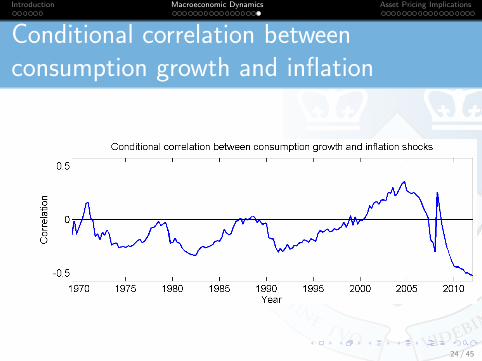
Introduction Macroeconomic Dynamics Asset Pricing Implications
Conditional correlation betweenconsumption growth and inflation
24 / 45

Introduction Macroeconomic Dynamics Asset Pricing Implications
Utility
Representative agent
Habit utility: E0
∑∞t=0 β
t (Ct−Ht)1−γ
1−γ
Discount factor β
”Risk-aversion” coefficient γ (always assumed >1)
Ct - consumption
Ht - external habit: e.g., exogeneous standard of living
25 / 45
Introduction Macroeconomic Dynamics Asset Pricing Implications
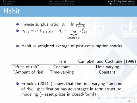
Habit
Inverse surplus ratio: qt = ln Ct
Ct−Ht
qt+1 = q + ρq(qt − q)− γq︸︷︷︸const>0
εgt+1
Habit = weighted average of past consumption shocks
Here Campbell and Cochrane (1999)”Price of risk” Constant Time-varying”Amount of risk” Time-varying Constant
Ermolov (2014a) shows that the time-varying ”amountof risk” specification has advantages in term structuremodeling (+asset prices in closed-form!)
26 / 45

Introduction Macroeconomic Dynamics Asset Pricing Implications
Financial Assets
Risk-free 0-coupon nominal bonds
Aggregate equity = claim to the
aggregate dividends
27 / 45
Introduction Macroeconomic Dynamics Asset Pricing Implications
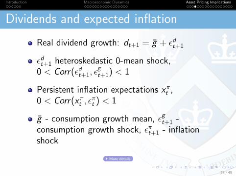
Dividends and expected inflation
Real dividend growth: dt+1 = g + εdt+1
εdt+1 heteroskedastic 0-mean shock,0 < Corr(εdt+1, ε
gt+1) < 1
Persistent inflation expectations xπt ,0 < Corr(xπt , ε
πt ) < 1
g - consumption growth mean, εgt+1 -consumption growth shock, επt+1 - inflationshock
More details
28 / 45
Introduction Macroeconomic Dynamics Asset Pricing Implications
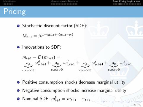
Pricing
Stochastic discount factor (SDF):
Mt+1 = βe−γgt+1+γ(qt+1−qt)
Innovations to SDF:
mt+1 − Et(mt+1) =ap︸︷︷︸
const<0
ωdp,t+1 + an︸︷︷︸
const>0
ωdn,t+1 + ap︸︷︷︸
const<0
ωsp,t+1 + an︸︷︷︸
const>0
ωsn,t+1
Positive consumption shocks decrease marginal utility
Negative consumption shocks increase marginal utility
Nominal SDF: m$t+1 = mt+1 − πt+1
29 / 45
Introduction Macroeconomic Dynamics Asset Pricing Implications
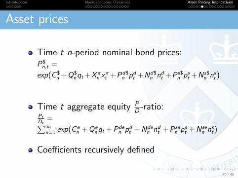
Asset prices
Time t n-period nominal bond prices:P$n,t =
exp(C $n +Q$
nqt +X πn x
πt +Pd$
n pdt +Nd$n ndt +P s$
n pst +N s$n nst )
Time t aggregate equity PD -ratio:
Pt
Dt=∑∞n=1 exp(C e
n +Qenqt +Pde
n pdt +Nden ndt +P se
n pst +N sen nst )
Coefficients recursively defined
30 / 45
Introduction Macroeconomic Dynamics Asset Pricing Implications
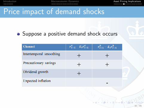
Price impact of demand shocks
Suppose a positive demand shock occurs
31 / 45
Introduction Macroeconomic Dynamics Asset Pricing Implications
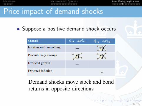
Price impact of demand shocks
Suppose a positive demand shock occurs
32 / 45
Introduction Macroeconomic Dynamics Asset Pricing Implications
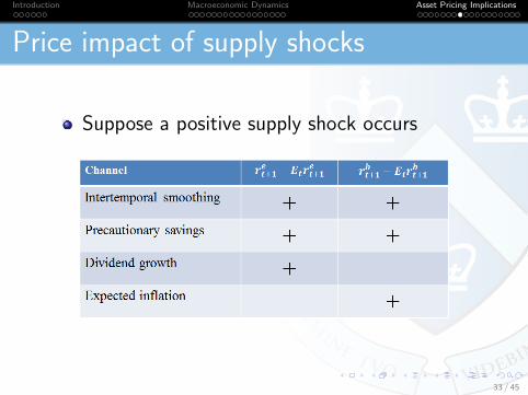
Price impact of supply shocks
Suppose a positive supply shock occurs
33 / 45
Introduction Macroeconomic Dynamics Asset Pricing Implications
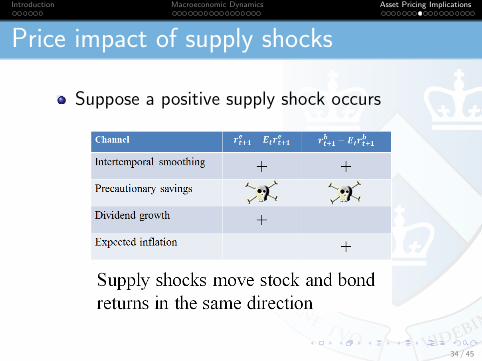
Price impact of supply shocks
Suppose a positive supply shock occurs
34 / 45
Introduction Macroeconomic Dynamics Asset Pricing Implications
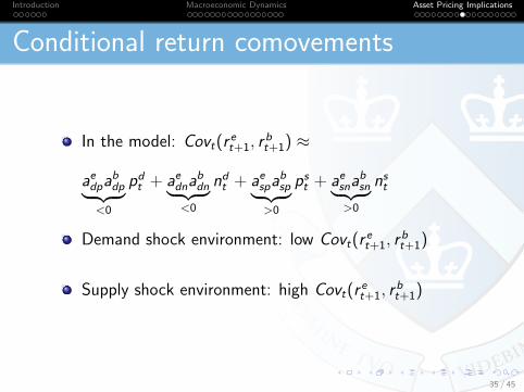
Conditional return comovements
In the model: Covt(ret+1, r
bt+1) ≈
aedpabdp︸ ︷︷ ︸
<0
pdt + aednabdn︸ ︷︷ ︸
<0
ndt + aespabsp︸ ︷︷ ︸
>0
pst + aesnabsn︸ ︷︷ ︸
>0
nst
Demand shock environment: low Covt(ret+1, r
bt+1)
Supply shock environment: high Covt(ret+1, r
bt+1)
35 / 45
Introduction Macroeconomic Dynamics Asset Pricing Implications
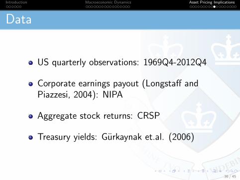
Data
US quarterly observations: 1969Q4-2012Q4
Corporate earnings payout (Longstaff andPiazzesi, 2004): NIPA
Aggregate stock returns: CRSP
Treasury yields: Gurkaynak et.al. (2006)
36 / 45
Introduction Macroeconomic Dynamics Asset Pricing Implications
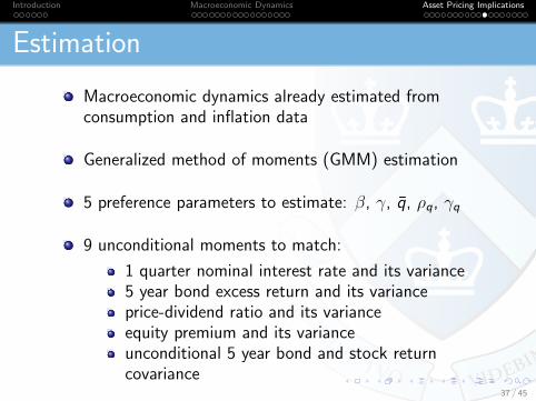
Estimation
Macroeconomic dynamics already estimated fromconsumption and inflation data
Generalized method of moments (GMM) estimation
5 preference parameters to estimate: β, γ, q, ρq, γq
9 unconditional moments to match:
1 quarter nominal interest rate and its variance5 year bond excess return and its varianceprice-dividend ratio and its varianceequity premium and its varianceunconditional 5 year bond and stock returncovariance
37 / 45
Introduction Macroeconomic Dynamics Asset Pricing Implications
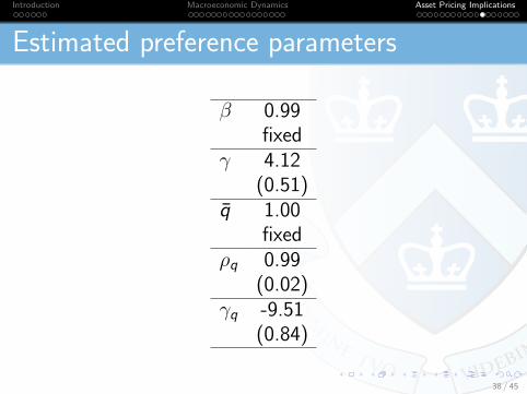
Estimated preference parameters
β 0.99fixed
γ 4.12(0.51)
q 1.00fixed
ρq 0.99(0.02)
γq -9.51(0.84)
38 / 45
Introduction Macroeconomic Dynamics Asset Pricing Implications
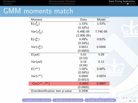
GMM moments matchMoment Data Model
E(y$1q) 1.33% 1.53%
(0.18%)
Var(y$1q) 6.48E-05 7.74E-05
(2.00E-05)E(rbx5y ) 0.49% 0.62%
(0.24%)Var(rbx5y ) 0.0011 0.0008
(0.0003)E(pd) 5.01 5.09
(0.10)Var(pd) 0.18 0.12
(0.04)E(r ex ) 1.08% 0.90%
(0.58%)Var(r ex ) 0.0085 0.0074
(0.0013)
Cov(r ex , rbx ) 0.0002 0.0007(0.0005)
Overidentification test p-value 0.2406
Implied macro moments Implied local risk-aversion Implied financial moments 39 / 45
Introduction Macroeconomic Dynamics Asset Pricing Implications
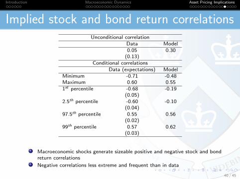
Implied stock and bond return correlationsUnconditional correlation
Data Model0.05 0.30
(0.13)Conditional correlations
Data (expectations) ModelMinimum -0.71 -0.48Maximum 0.60 0.551st percentile -0.68 -0.19
(0.05)2.5th percentile -0.60 -0.10
(0.04)97.5th percentile 0.55 0.56
(0.02)99th percentile 0.57 0.62
(0.03)
Macroeconomic shocks generate sizeable positive and negative stock and bondreturn correlations
Negative correlations less extreme and frequent than in data
40 / 45
Introduction Macroeconomic Dynamics Asset Pricing Implications
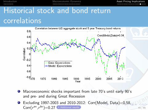
Historical stock and bond returncorrelations
Macroeconomic shocks important from late 70’s until early 90’sand pre- and during Great Recession
Excluding 1997-2003 and 2010-2012: Corr(Model, Data)=0.58,Corr(r ex ,rbx)=0.27 Additional results 41 / 45
Introduction Macroeconomic Dynamics Asset Pricing Implications
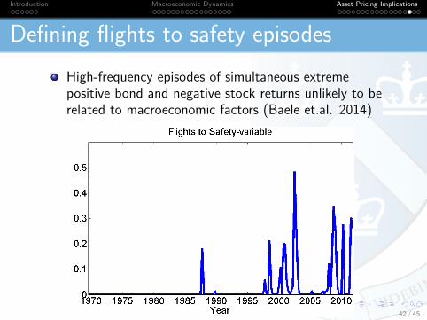
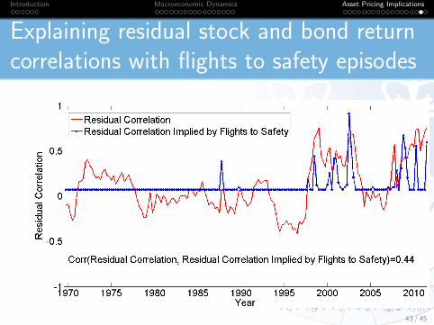
Defining flights to safety episodes
High-frequency episodes of simultaneous extremepositive bond and negative stock returns unlikely to berelated to macroeconomic factors (Baele et.al. 2014)
42 / 45
Introduction Macroeconomic Dynamics Asset Pricing Implications
Explaining residual stock and bond returncorrelations with flights to safety episodes
43 / 45

Introduction Macroeconomic Dynamics Asset Pricing Implications
Comparision to the literature
Studies finding weak links between risk ofnominal assets and macroeconomy: restrictivemacroeconomic dynamics (difficult toincorporate realistic dynamics into asset pricingframeworks in a tractable manner)
Studies finding strong links between risk ofnominal assets and macroeconomy: rely onfinancial data to estimate macroeconomicshocks
44 / 45

Introduction Macroeconomic Dynamics Asset Pricing Implications
Conclusions
Tractable structural framework for understandingmacroeconomic risk of nominal assets: tons ofapplications!
Economically characterizing macroeconomic shocks
Macroeconomic shocks:
produce sizeable positive and negative stock andbond return correlations, although negativecorrelations smaller and less frequent than in datahistorically most important for correlations fromlate 70’s to early 90’s and pre- and during theGreat Recession
45 / 45

Appendix 1: BEGE conditional moments
Intuitive theoretical expressions for (unscaled)moments:
Vart(ut+1) = σ2ppt + σ2
nnt
Skwt(ut+1) = 2(σ3ppt − σ3
nnt)
Ex .Kurt(ut+1) = 6(σ4ppt + σ4
nnt)
Back
46 / 45
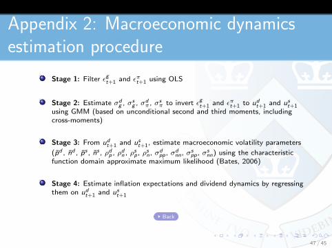
Appendix 2: Macroeconomic dynamicsestimation procedure
Stage 1: Filter εgt+1 and επt+1 using OLS
Stage 2: Estimate σdg , σs
g , σdπ , σs
π to invert εgt+1 and επt+1 to udt+1 and ust+1using GMM (based on unconditional second and third moments, includingcross-moments)
Stage 3: From udt+1 and ust+1, estimate macroeconomic volatility parameters
(pd , nd , ps , ns , ρdp , ρdn , ρsp , ρsn, σdpp , σd
nn, σspp , σs
nn) using the characteristicfunction domain approximate maximum likelihood (Bates, 2006)
Stage 4: Estimate inflation expectations and dividend dynamics by regressingthem on udt+1 and ust+1
Back
47 / 45
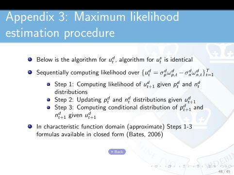
Appendix 3: Maximum likelihoodestimation procedure
Below is the algorithm for udt , algorithm for ust is identical
Sequentially computing likelihood over {udt = σdpω
dp,t −σd
nωdn,t}Tt=1
Step 1: Computing likelihood of udt+1 given pdt and ndtdistributionsStep 2: Updating pdt and ndt distributions given udt+1
Step 3: Computing conditional distribution of pdt+1 andndt+1 given udt+1
In characteristic function domain (approximate) Steps 1-3formulas available in closed form (Bates, 2006)
Back
48 / 45
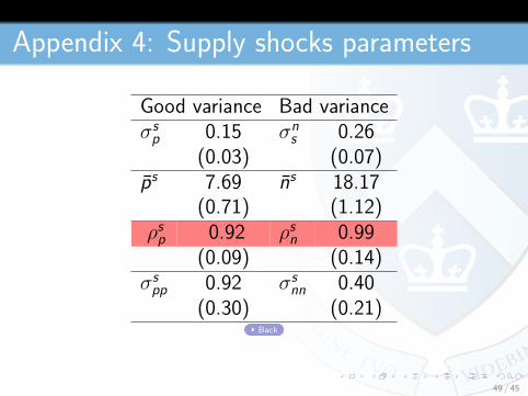
Appendix 4: Supply shocks parameters
Good variance Bad varianceσsp 0.15 σns 0.26
(0.03) (0.07)ps 7.69 ns 18.17
(0.71) (1.12)ρsp 0.92 ρsn 0.99
(0.09) (0.14)σspp 0.92 σsnn 0.40
(0.30) (0.21)Back
49 / 45
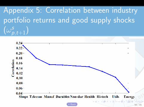
Appendix 5: Correlation between industryportfolio returns and good supply shocks(ωs
p,t+1)
Back 50 / 45
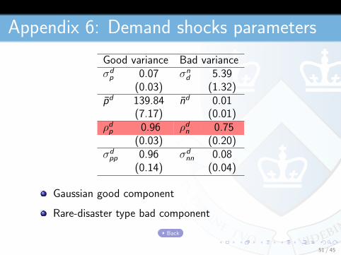
Appendix 6: Demand shocks parameters
Good variance Bad varianceσdp 0.07 σn
d 5.39(0.03) (1.32)
pd 139.84 nd 0.01(7.17) (0.01)
ρdp 0.96 ρdn 0.75(0.03) (0.20)
σdpp 0.96 σd
nn 0.08(0.14) (0.04)
Gaussian good component
Rare-disaster type bad component
Back
51 / 45
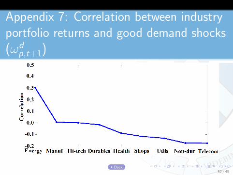
Appendix 7: Correlation between industryportfolio returns and good demand shocks(ωd
p,t+1)
Back52 / 45
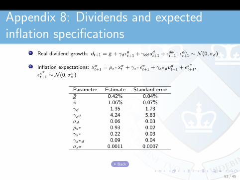
Appendix 8: Dividends and expectedinflation specifications
Real dividend growth: dt+1 = g + γd εgt+1 + γddu
dt+1 + εdivt+1, ε
divt+1 ∼ N (0, σd )
Inflation expectations: xπt+1 = ρxπ xπt + γxπ επt+1 + γxπdudt+1 + εx
π
t+1,
εxπ
t+1 ∼ N (0, σπx )
Parameter Estimate Standard errorg 0.42% 0.04%π 1.06% 0.07%γd 1.35 1.73γdd 4.24 5.83σd 0.06 0.03ρxπ 0.93 0.02γxπ 0.22 0.03γxπd 0.09 0.04σxπ 0.0011 0.0007
Back
53 / 45
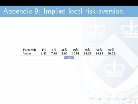
Appendix 9: Implied local risk-aversion
Percentile 1% 5% 25% 50% 75% 95% 99%Value 6.33 7.30 8.99 10.58 13.02 19.85 29.23
Back
54 / 45
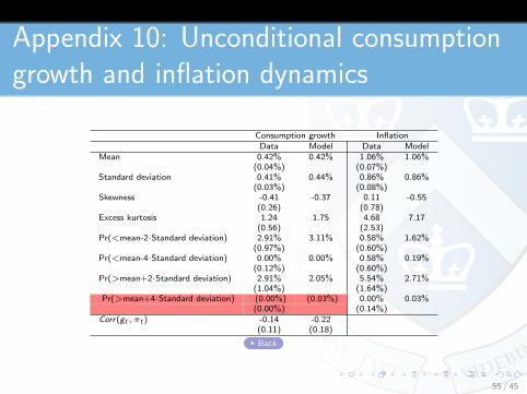
Appendix 10: Unconditional consumptiongrowth and inflation dynamics
Consumption growth InflationData Model Data Model
Mean 0.42% 0.42% 1.06% 1.06%(0.04%) (0.07%)
Standard deviation 0.41% 0.44% 0.86% 0.86%(0.03%) (0.08%)
Skewness -0.41 -0.37 0.11 -0.55(0.26) (0.78)
Excess kurtosis 1.24 1.75 4.68 7.17(0.56) (2.53)
Pr(<mean-2·Standard deviation) 2.91% 3.11% 0.58% 1.62%(0.97%) (0.60%)
Pr(<mean-4·Standard deviation) 0.00% 0.00% 0.58% 0.19%(0.12%) (0.60%)
Pr(>mean+2·Standard deviation) 2.91% 2.05% 5.54% 2.71%(1.04%) (1.64%)
Pr(>mean+4·Standard deviation) (0.00%) (0.03%) 0.00% 0.03%(0.00%) (0.14%)
Corr(gt , πt ) -0.14 -0.22(0.11) (0.18)
Back
55 / 45
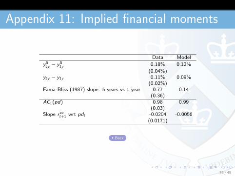
Appendix 11: Implied financial moments
Data Model
y$5y − y$
1y 0.18% 0.12%
(0.04%)y5y − y1y 0.11% 0.09%
(0.02%)Fama-Bliss (1987) slope: 5 years vs 1 year 0.77 0.14
(0.36)AC1(pd) 0.98 0.99
(0.03)Slope r ext+1 wrt pdt -0.0204 -0.0056
(0.0171)
Back
56 / 45
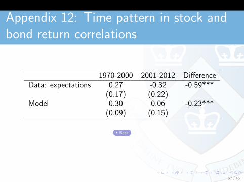
Appendix 12: Time pattern in stock andbond return correlations
1970-2000 2001-2012 DifferenceData: expectations 0.27 -0.32 -0.59***
(0.17) (0.22)Model 0.30 0.06 -0.23***
(0.09) (0.15)
Back
57 / 45