1  

         

 

Title: Urbanization Policy in Malaysia and its Impacts Author: Louise Duflot Date: December 2012 Institution name/journal where submitted: McGill University

The use of this database indicates agreement to the terms and conditions Academia is a database that promotes the free exchange of exceptional ideas and scholarly work, setting a platform on which to foment and improve student discourse                                

             

 

2  

Having lived in Singapore for six years, I had always been amazed by the spatial organization

of the city-state. Everything has been ordered and organized so that the town functions

effectively, with highways all around the city centre, enabling the traffic to be regulated as

well as with neighbourhoods where you find everything a household needs so that you do not

need to take your car to go to the groceries. And when you do, the public transport system of

buses and subway lines enables you to travel around the island easily.

Even though Singapore is physically located in South East Asia, it defers greatly from its

neighbours, a difference that is striking. You just have to cross the 1km bridge separating

Singapore from the capital of the state of Johor, Johor Bahru in Malaysia to notice this

difference. Suddenly, you feel like you’ve entered an chaotis town, which developed

anarchically and is congested with traffic and pollution.

Whereas Singapore is the symbol of a western style developed, high income country,

Malaysia as a newly industrialized country (NIC) is still considered a developing country.

Because I have always lived in European or North American-style developed cities but have

travelled abundantly in developing countries all across Asia, I chose to do my research paper

on Malaysia, in order to understand better the pattern of urbanization of my neighbouring

country.

Concerning the time period I chose for my research: 1970s to 2000s (even if some data may

cover some very recent developments) is a strategic choice corresponding to the launch of the

New Economic Policy (NEP) in 1971 which had enormous consequences on the development

of the country, including urbanization. The NEP ended in 1990, but it remains very

interesting to examine the evolution of the development trends after such intense government

backed policies ended.

Urbanization is the shift from a rural to an urban society. Urbanization is therefore

 

3  

characterized by a rural-urban migration of people, which leads to an increase in the number

of people living in urban areas, such as cities. The causes of urbanization are various but

people often migrate to urban areas in order to find work, escape famines... Therefore

urbanization leads to the development of large urban conurbations and has implications on

people’s patterns of life and habits. It leads to both an adaptation from the people who

migrate as well as an adaptation of the landscape and organization of the city to respond the

best it can to its new inhabitants’ needs.

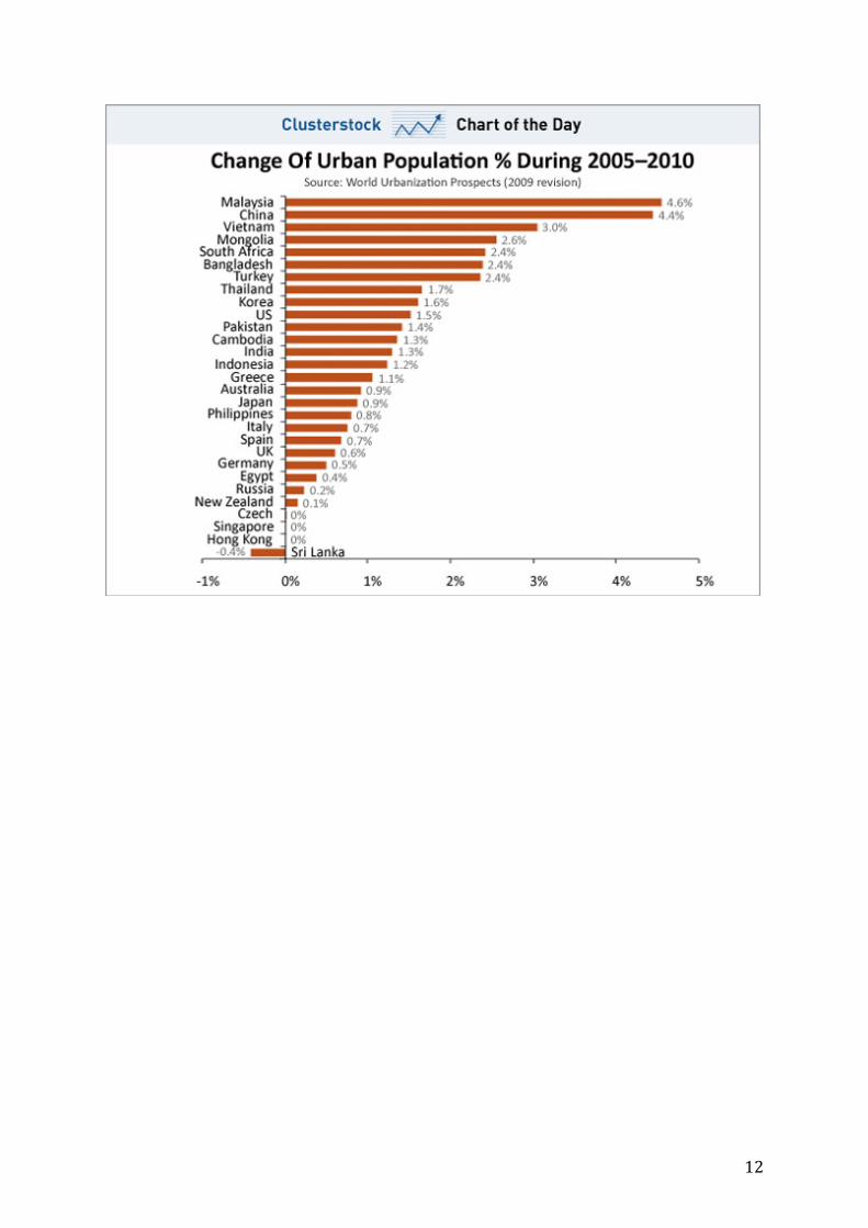
Malaysia has achieved remarkable economic growth since its independence in 1957 and is

now one of the most urbanized developing countries in the world. Its rate of urbanization is

so rapid that cities are growing more rapidly in Malaysia than in China. (see FIGURE 1) and

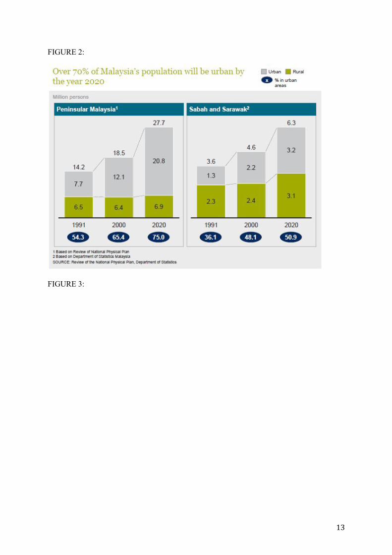
if this trend continues, over 70% of the Malaysian population will be urban by 2020

(FIGURE 2). Like any developing country, Malaysia has experienced and still experiences

urbanization that translates itself by expanding city sizes around the country. Urban dwellers

move towards the cities because they are looking for better living conditions such as access to

potable water supply, access to various health services as well as securing gainful

employment (FIGURE 3).

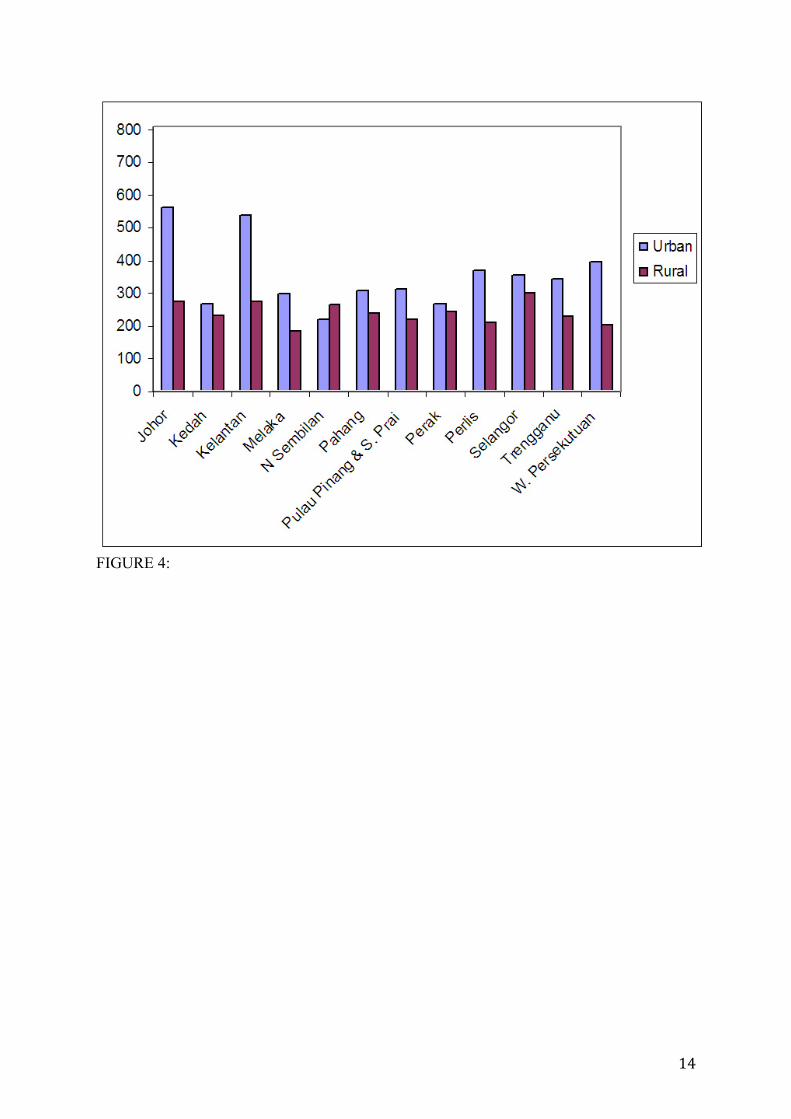
Between 1970 and 2000, the urban population ratio in Malaysia grew from 26.8% to 61.8%

with a more pronounced increase between 1980 and 2000 (see FIGURE 4). And this growth

of urban population is sustained, since in 2010, an estimated of 72% of the Malaysian

population lived in urban areas. Indeed, according to the CIA website, the annual rate of

change of the rate of urbanization between 2010 and 2015 is estimated to be of 2.4%.

There are three components of urban growth that are significant into explaining the extent of

urbanization in Malaysia; these are: natural increase, rural-urban migration with the policies

 

4  

that affected it, and reclassification of rural areas and agglomeration of built-up areas.

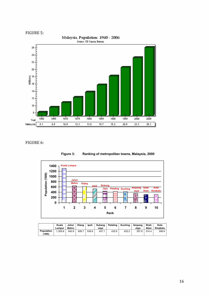
Natural increase refers to the natural population growth that the country experiences. Indeed,

if we look at the data, the population of Malaysia was of 13,879,252 in 1980 and of

27,468,000 in 2000. As a result, the cities grow. (see FIGURE 5)

Like in any other country, the cities in Malaysia developed because of the growth of industry

and the development of the manufacturing sector, particularly during the NEP in Malaysia.

During the NEP, which lasted from 1971 to 1990, the government sought to restructure

society. Indeed, the Malaysian government wanted to bring about a more balanced

participation of the different ethnic groups in the economy, more importantly by giving more

power to the Bumiputera who are the indigenous Malays and urbanize them. Therefore the

period of the NEP has been one of intense migrations in the country with Malays becoming

the largest urban migrants among the different ethnic communities of the country. In order to

promote this urbanization of the Bumiputera the Malays were offered several incentives such

as scholarships, loans to set up businesses. These policies were indeed successful because

the Malays went from representing 17% of the urban population in the 60s to 44% in 2000.

As we have mentioned before, between 1970 and 2004, the number of urban dwellers in

Malaysia went from 2.96 million to 16.44 million. Migration accounted for 40% of urban

growth in Selangor and Kuala Lumpur. The inflow of migrants from the rural to the urban

areas accounted for about 30% of urban population growth in Malaysia from the 70s to the

early 2000s.

It is also important to remember that in Malaysia, urbanization was common to all states

unlike in other Southeast Asian countries where an all-dominant megacity such as Jakarta or

Bangkok emerged as a result of urbanization. In Malaysia, in 2000, all states had at least 1/3

 

5  

of their population residing in urban areas. The Federal State of Kuala Lumpur was the most

urbanized with a 100% of the territory considered urban, followed by Selangor with 88.3%

and Penang with 79.5%. Also, it is important to remember that regionally, Peninsular

Malaysia is more urbanized than Sabah and Sarawak, even though these states are still 50%

urbanized. (see FIGURES 6&7)

As for explaining this migration with economic models such as the Harris-Todaro model or

the Lewis Dual Sector model, we have to be careful on the assumptions that we take into

account. Indeed the Harris-Todaro model assumes that people migrate from rural areas to

urban ones because they are motivated by rational economic considerations of relative

benefits and the decision to migrate depends on expected wages rather than actual wage

differential between the 2 sectors. In Malaysia, it is important to remember that the primary

incentives to migrate were given by the government who encouraged Malays to move to the

cities by providing them with financial incentives. These financial incentives helped them set

up their businesses and therefore ensured them substantially better living conditions than the

ones they had in the countryside. Therefore, I think it is significant to apply the Harris-

Todaro model to the migration process in Malaysia. The NEP reform promised benefits to

the migrants and they were therefore motivated to migrate by the higher wages that would be

offered to them in the cities.

The third variable concerns the classification of urban areas that has changed over the years

in the country. Indeed, before 1970, the definition of urban areas used in the population

censuses referred to areas comprised of local administrative units with a population of 1,000

persons or above. But after 1970, the minimum population for an area to be considered urban

was increased to 10,000. This change was to reflect a more realistic level of urbanization

because areas with population below this size displayed rural socio-economic characteristics,

 

6  

and keeping the threshold at 1,000 would have over-emphasized the level of urbanization of

the country.

These 3 variables offer a comprehensive view of the different factors motivating the

development of cities in the country. Even though the natural increase of population and the

modification of certain urbanization definitions are significant, the second variable

concerning the rural-urban migration motivated by the NEP and the movement of the

economy from an agricultural based on to a highly effective manufacturing one is the most

important variable explaining the growth of the cities in Malaysia.

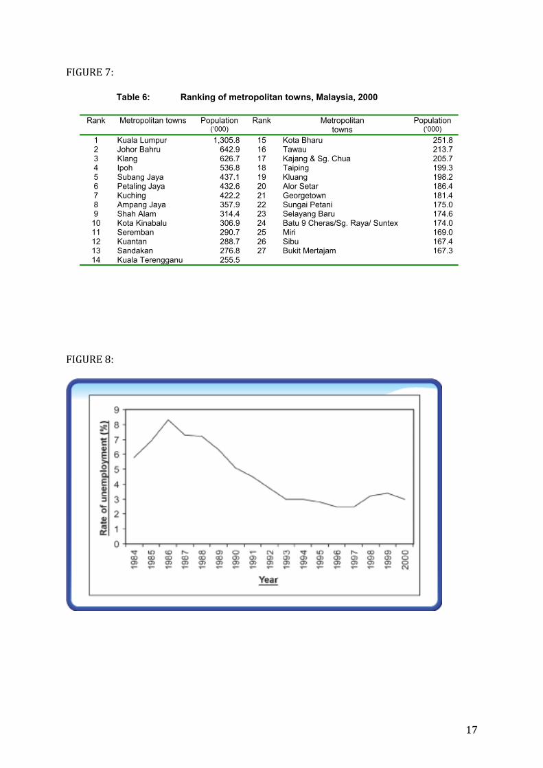
We can therefore see that in the case of Malaysia, the rate of unemployment moves in the

opposite direction as the rate of urbanization. Even though urbanization continues to

progress, the rate of unemployment in the country has decreased.

The fact that people still migrate to cities and that they are not unemployed means that

there are jobs in Malaysia. If we refer to the Lewis Dual Sector model it then means that the

threshold point where all the surplus labour of the traditional sector has been absorbed by the

manufacturing is not yet reached. The manufacturing sector still has resources to offer to job

seekers and so people continue to migrate. This continuous migration can be explained by the

growth of GDP and the allocation of GDP shares per sectors in the economy.

In Malaysia, the rate of unemployment in 1985 was of 6.893% and it decreased to 3.002% in

2000. If we look at the data from 2010, we can see that the rate of unemployment has increased

slightly to 3.3% but this increase can be attributed to the actual international economic and

financial situation of the times (see FIGURE 8)

 

7  

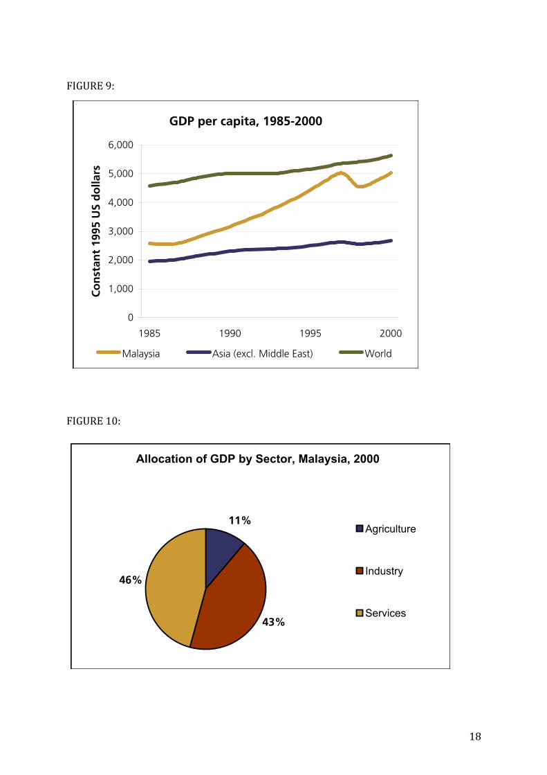
Indeed, from 1980 until 2010, Malaysia's average GDP per capita PPP was 7460.92 dollars

reaching an historical high of 14730.93 dollars in December of 2010 and a record low of

2336.21 dollars in December of 1980. When looking at FIGURE 9, it seems that Malaysia’s

GDP per capita has been growing steadily since 1980, therefore following the trend of the

rate of urbanization.

We know that when a country develops, it urbanizes but we also know that its allocation of

GDP per sector shifts in the process. Indeed the process of urbanization illustrates a major

shift from the agricultural to the manufacturing sector, but it is not because all the surplus

rural labour has been absorbed that the economy stops developing. Indeed, once the

manufacturing sector has been developed and its productivity is sustained, the economy

continues to develop and the service sector starts to be more and more important in terms of

share allocation in the GDP. This is what happened in Malaysia. (see FIGURE 10) The

service sector develops itself, and services are located in cities. Indeed Kuala Lumpur is

considered one of the most important financial centres in the Arab world and many

international banks and telecommunications companies set up offices in Malaysia. This can

therefore explain the continuous increase in urbanization and the fact that unemployment

does not increase: people continue to migrate because they find job in the services sector

(FIGURE 6).

As urbanization occurred, the economy and the country developed. Migration occurs from

the rural to the urban sector because people are attracted by the higher wages offered by the

industrial sector. While developing, economies follow a certain trend where their GDP is less

and less dependent on agriculture and more and more on the manufacturing sector. After this,

another shift occurs where the services sector develops to become a prominent contributor to

GDP.

 

8  

Urbanization can have a positive impact on development issues such as poverty, inequality

and environmental degradation, so long as the appropriate policies are in place to manage the

problems and challenges that come from this intense process.

The urbanization of Malaysia from a rural agrarian based economy to an urban based one has

lifted the income levels and living standards of both the rural and the urban sectors.

Following the Lewis dual sector model, much of the excess labour that was located in the

rural areas and occupied the low productivity sectors has been moved to urban and higher

productivity sectors, which means that the migrants have acquired new skills.

It is important to remember that many policy implications of migration theories such as the

Harris-Todaro model assume that the consequence of such migration will be urban bias. But

this is not what happened in Malaysia, even though the percentage of migration in Kuala

Lumpur has been substantially important, major cities develop in each states of the country as

we can see in FIGURES 6&7.

This can be explained by the NEP Policy: because the government was behind such a

process, it was able to regulate the migration and offer jobs and opportunities in all states

equally so that the migration would be inter-state rather than intra-state. When we know that

a negative consequence of urbanization and migration is that people often leave their

hometowns for good and do not come back, in Malaysia, people were not completely

uprooted from their hometowns and stayed within their home-states.

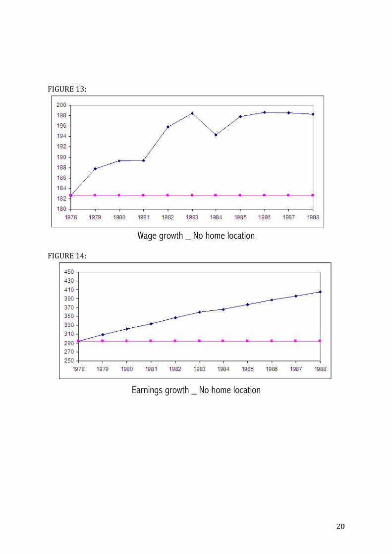
Furthermore, one important benefit of urbanization was that wages and earnings increased for

the people who migrated. FIGURE 11 shows the wage growth for a person at his home

location and FIGURE 12 the earnings growth. We can see that by staying at their home

locations, these people are not likely to experience any significant increase in either wages or

earnings. In contrast, by looking at FIGURES 13&14 which represent people with no home

 

9  

locations we can see that these persons will be much more likely to migrate in response to

wage differentials. They will have significant increases in their earnings and wages. This

shows that the preference for remaining at home explains why people are not experiencing

much wage growth through migration.

Also, overall, urbanization has decreased the degree of inequality in Malaysia, indeed, one of

the main problems in Malaysia was the glaring disparities between the different ethnic

groups. For example, when we see FIGURE 15, we can see that during the migration period,

the GINI coefficient has decreased in Malaysia, reducing income inequality.

Even if urbanization’s main benefits are to improve peoples’ living standards, urbanization

can also have negative impacts. The rapid growth of the urban population exerts pressures on

the provision of adequate housing, sanitary facilities, proper drainage, garbage disposal,

health and educational facilities… In Kuala Lumpur, three main issues which are direct

consequences of urbanization are at stake: the existence of some 300,000 squatters; the

shortage of low cost housing for low income workers (many immigrants workers come in

from Pakistan and Bangladesh to work on construction cites and they are not well hosted);

the emergence of urban slum areas in the cities and the suburbs... In this regard, the

Malaysian Government has to undertake projects related to these aspects including

environmental issues such as water pollution caused by increased urbanization and expanding

industries.

Another important consequence is that all the youth move to the cities and therefore the youth

population in villages remains at about 10% to 15%, villages are therefore being deprived of

able persons to pursue the different programs of rural modernization. Therefore the

government should concentrate on improving the work opportunities in rural areas and

overcoming the imbalance in socioeconomic life between rural and urban areas. The NEP

 

10  

encouraged urbanization in Malaysia in order to re-balance wages and opportunities between

the different ethnic groups but the goal has never been to completely deplete the countryside

of all its population.

These issues illustrate the fact that even though urbanization is a mandatory step toward

modernization and development for developing countries, it is a complex process that needs

to be addressed and monitored by the state at all times.

Bibliography

"Malaysia Urbanization." - Demographics. Web. 02 Mar. 2012. <http://www.indexmundi.com/malaysia/urbanization.html>. "Malaysia." Data. Web. 02 Mar. 2012. <http://data.worldbank.org/country/malaysia>. "Between the Poles." Between the Poles. Web. 02 Mar. 2012. <http://geospatial.blogs.com/>. "Featured Articles from Business Insider." Featured Articles From The Business Insider. Web. 17 Feb. 2011 <http://articles.businessinsider.com>. "Supplemental Content." National Center for Biotechnology Information. U.S. National Library of Medicine. Web. 02 Mar. 2012. <http://www.ncbi.nlm.nih.gov/pubmed/12336534>. "Internal Migration in Malaysia: Spatial and Temporal Analysis." GIS and Science. Web. 02 Mar. 2012. <http://gisandscience.com/2011/03/22/internal-migration-in-malaysia-spatial-and-temporal-analysis/>.

 

11  

"URBANIZATION AND URBAN MIGRANTS IN MALAYSIA: A COMPARATIVE STUDY BETWEEN CHINESE AND MALAYS”. Web. 02 Mar. 2012. <http://www.malaysian-chinese.net/publication/articlesreports/articles/8378.html>. "Economy Watch - Follow The Money." World, US, China, India Economy, Investment, Finance, Credit Cards. Web. 02 Mar. 2012. <http://www.economywatch.com>. "The Official Website of Department of Statistics Malaysia." Welcome to the Department of Statistics Official Website. Web. 02 Mar. 2012. <http://www.statistics.gov.my/portal/index.php?lang=en>. "Association of National Census and Statistics Directors of America, Asia and the Pacific." Association of National Census and Statistics Directors of America, Asia and the Pacific. Web. 02 Mar. 2012. <http://www.ancsdaap.org/>. "The Official Website of the Association of Southeast Asian Nations." The Official Website of the Association of Southeast Asian Nations. Web. 04 Mar. 2012. <http://www.asean.org/>. "EarthTrends | Environmental Information." EarthTrends. Web. 04 Mar. 2012. <http://earthtrends.wri.org/>.

Appendixes

FIGURE 1:

 

12  

 

13  

FIGURE 2:

FIGURE 3:

 

14  

FIGURE 4:

 

15  

                           

45

Table 1: Urbanisation levels, urban population growth and tempo of urbanisation, Malaysia

Year Proportion

of population in urban areas

(per cent)

Average annual intercensal population growth rate

(per cent)

Tempo of urbanisation

(per cent)

Malaysia 1970 1980 1991 2000

26.8 35.8 (34.2) 50.7 61.8

: 5.2 (3.0) 5.8 (6.2) 4.8

: 2.9 (2.4) 3.2 (3.6) 2.2

Footnote: Figures in parenthesis refer to data released earlier in the official census reports.

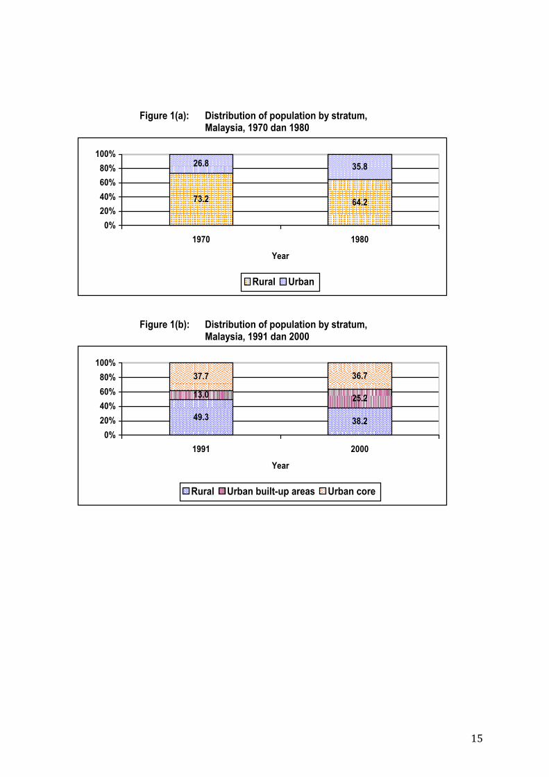
Figure 1(a): Distribution of population by stratum, Malaysia, 1970 dan 1980

73.2 64.2

26.8 35.8

0%20%40%60%80%

100%

1970 1980

Year

Rural Urban

Figure 1(b): Distribution of population by stratum, Malaysia, 1991 dan 2000

49.3 38.2

37.7 36.7

13.0 25.2

0%20%40%60%80%

100%

1991 2000

Year

Rural Urban built-up areas Urban core

Variations in the rate of urban population growth provide another dimension on the nature of the change in the level of urbanisation over time. A commonly used indicator of urban population growth is the tempo of urbanisation which is a measure of the difference in the growth rate of the urban population and that of the total population. The urban growth rates and tempo of urbanisation during the intercensal periods are also shown in Table 1.

 

16  

 FIGURE  5:  

     FIGURE  6:    

       

51

Table 6: Ranking of metropolitan towns, Malaysia, 2000

Rank Metropolitan towns Population

(‘000) Rank Metropolitan

towns Population

(‘000) 1 Kuala Lumpur 1,305.8 15 Kota Bharu 251.8 2 Johor Bahru 642.9 16 Tawau 213.7 3 Klang 626.7 17 Kajang & Sg. Chua 205.7 4 Ipoh 536.8 18 Taiping 199.3 5 Subang Jaya 437.1 19 Kluang 198.2 6 Petaling Jaya 432.6 20 Alor Setar 186.4 7 Kuching 422.2 21 Georgetown 181.4 8 Ampang Jaya 357.9 22 Sungai Petani 175.0 9 Shah Alam 314.4 23 Selayang Baru 174.6 10 Kota Kinabalu 306.9 24 Batu 9 Cheras/Sg. Raya/ Suntex 174.0 11 Seremban 290.7 25 Miri 169.0 12 Kuantan 288.7 26 Sibu 167.4 13 Sandakan 276.8 27 Bukit Mertajam 167.3 14 Kuala Terengganu 255.5

In 2000, Kuala Lumpur was the primate city with a population size of almost two times that of the next two largest cities, Johor Bahru and Klang (Figure 3). It is also noted that some of these largest metropolitan towns are also state capitals.

Figure 3: Ranking of metropolitan towns, Malaysia, 2000

Ampang

JayaKuchingPetaling

Subang

JayaIpoh

Klang

Johor

Bahru

Kota

Kinabalu

Shah

Alam

Kuala Lumpur

0

200

400

600

800

1000

1200

1400

1 2 3 4 5 6 7 8 9 10

Rank

Po

pu

lati

on

('0

00)

Kuala

Lumpur

Johor

Bahru

Klang Ipoh Subang

Jaya

Petaling Kuching Ampang

Jaya

Shah

Alam

Kota

Kinabalu Population

(‘000) 1,305.8 642.9 626.7 536.8 437.1 432.6 422.2 357.9 314.4 306.9

In the study of urbanisation, it is important to understand the relationship of primate urban centre and other urban centres. This relationship can be summarised by an index known as Primacy Index (PI). This index is related to the rank-size rule and measures the concentration of population in the primate city in relation to the rest of the other cities. The greater the index value, the greater is the concentration in the largest city. For a group of cities/towns, the PI is the quotient of the largest city divided by the summation of the population of the second and subsequent cities. The rank-size rule means that the second-ranked city is half the population size of the primate city, the third-ranked city is one-third in size and so on.

 

17  

FIGURE  7:

             FIGURE  8:    

               

51

Table 6: Ranking of metropolitan towns, Malaysia, 2000

Rank Metropolitan towns Population

(‘000) Rank Metropolitan

towns Population

(‘000) 1 Kuala Lumpur 1,305.8 15 Kota Bharu 251.8 2 Johor Bahru 642.9 16 Tawau 213.7 3 Klang 626.7 17 Kajang & Sg. Chua 205.7 4 Ipoh 536.8 18 Taiping 199.3 5 Subang Jaya 437.1 19 Kluang 198.2 6 Petaling Jaya 432.6 20 Alor Setar 186.4 7 Kuching 422.2 21 Georgetown 181.4 8 Ampang Jaya 357.9 22 Sungai Petani 175.0 9 Shah Alam 314.4 23 Selayang Baru 174.6 10 Kota Kinabalu 306.9 24 Batu 9 Cheras/Sg. Raya/ Suntex 174.0 11 Seremban 290.7 25 Miri 169.0 12 Kuantan 288.7 26 Sibu 167.4 13 Sandakan 276.8 27 Bukit Mertajam 167.3 14 Kuala Terengganu 255.5

In 2000, Kuala Lumpur was the primate city with a population size of almost two times that of the next two largest cities, Johor Bahru and Klang (Figure 3). It is also noted that some of these largest metropolitan towns are also state capitals.

Figure 3: Ranking of metropolitan towns, Malaysia, 2000

Ampang

JayaKuchingPetaling

Subang

JayaIpoh

Klang

Johor

Bahru

Kota

Kinabalu

Shah

Alam

Kuala Lumpur

0

200

400

600

800

1000

1200

1400

1 2 3 4 5 6 7 8 9 10

Rank

Po

pu

lati

on

('0

00)

Kuala

Lumpur

Johor

Bahru

Klang Ipoh Subang

Jaya

Petaling Kuching Ampang

Jaya

Shah

Alam

Kota

Kinabalu Population

(‘000) 1,305.8 642.9 626.7 536.8 437.1 432.6 422.2 357.9 314.4 306.9

In the study of urbanisation, it is important to understand the relationship of primate urban centre and other urban centres. This relationship can be summarised by an index known as Primacy Index (PI). This index is related to the rank-size rule and measures the concentration of population in the primate city in relation to the rest of the other cities. The greater the index value, the greater is the concentration in the largest city. For a group of cities/towns, the PI is the quotient of the largest city divided by the summation of the population of the second and subsequent cities. The rank-size rule means that the second-ranked city is half the population size of the primate city, the third-ranked city is one-third in size and so on.

 

18  

 FIGURE  9:  

       FIGURE  10:    

   

Gross Domestic Product, 2000 MalaysiaAsia (excl.

Middle East) WorldGDP in million constant 1995 US dollars 111,617 8,913,075 34,109,900GDP PPP (million current international dollars) {a} 211,019 14,443,434 44,913,910Gross National Income (PPP, in million current

international dollars), 2000 {a} 193,914 14,332,825 44,458,520GDP per capita, 2000

in 1995 US dollars 5,024 2,670 5,632in current international dollars 9,497 4,327 7,416

Average annual growth in GDP, 1991-2000Total 6% 3% 3%Per capita 5% 1% 1%

Percent of GDP earned by:Agriculture, 2000 11% X XIndustry, 2000 45% X XServices, 2000 44% X X

International TradeTrade in Goods and Services (million current $US)

Imports, 2000 94,618 819,978 XExports, 2000 112,513 895,412 X

Exports as a percent of GDP, 2000 125% X XBalance of Trade, 2000 (million current $US) 18,947 X X

Official Development Assistance (ODA ) and Financial FlowsODA in million US dollars, 1998-2000 {b} 133 X 59,073ODA per capita in US dollars, 1998-2000 {b} 6 4 10Current Account Balance (million $US), 2000 X X XTotal external debt, million $US, 1998-2000 {b} 42,036 X XDebt service as a % of export earnings, 1995-97 {b} 7.8% X XForeign Direct Investment, net inflows

(million current $US), 2000 1,660 71,197 XInternational Tourism Receipts,

1995-1997 (million $US) 3,895 X X

Economic Indicators -- Malaysia

View more Country Profiles on-line at http://earthtrends.wri.org

Gross Domestic Product, Malaysia, 1975-2000

0

20,000

40,000

60,000

80,000

100,000

120,000

140,000

160,000

180,000

200,000

1975 1980 1985 1990 1995 2000

Mill

ions

of

Dol

lars

million constant US$ million $intl (PPP)

GDP per capita, 1985-2000

0

1,000

2,000

3,000

4,000

5,000

6,000

1985 1990 1995 2000

Cons

tant

199

5 U

S do

llars

Malaysia Asia (excl. Middle East) World

EarthTrendsCountry Profiles

© EarthTrends 2003. All rights reserved. Fair use is permitted on a limited scale and for educational purposes. page 1

MalaysiaAsia (excl.

Middle East) WorldNational Savings (as a percent of Gross National Income)Gross National Savings, 2000 42% 30% 23%Net National Savings, 2000 30% 17% XAdjusted Net Savings, 2000 23% 19% X

Income Distribution (years vary)Gini coefficient (0=perfect equality;

100=perfect inequality) 49 X XPercent of total income earned by the richest

20% of the population: 54.3% X XPercent of total income earned by the poorest

20% of the population: 4.4% X XNational Poverty Rate 15.5% X XPoverty Rate, Urban Population X X XPercent of population living on less than $1 a day X X XPercent of population living on less than $2 a day X X X

Other Resources:Country Profiles of the Food and Agriculture Organization

of the United Nations, Economic Situation:http://www.fao.org/fi/fcp/en/MYS/profile.htm

a. Data are in international dollars, adjusted for purchasing power parity (PPP). PPP rates provide a standard measure allowing comparison of real

price levels between countries. b. Data are averaged for the range of years listed.

Economic Indicators -- Malaysia

View more Country Profiles on-line at http://earthtrends.wri.org

Allocation of GDP by Sector, Malaysia, 2000

11%

43%

46%

Agriculture

Industry

Services

0

10

20

30

40

50

60

poorest richest

Quintile of Population

Perc

ent o

f Tot

al In

com

e

Distribution of Income, Malaysia

© EarthTrends 2003. All rights reserved. Fair use is permitted on a limited scale and for educational purposes. page 2

 

19  

   FIGURE  11:    

Wage growth _ At home location    FIGURE  12:    

Earnings growth _ At home location                          

FIGURE 2: WAGE GROWTH- AT HOME LOCATION

FIGURE 3: EARNINGS GROWTH- AT HOME LOCATION

lines represent the earnings of a person who can migrate. There is no trend in wagesbut earnings slope slightly upward.

I next perform the same exercise for a person who does not have a home location.This person will be much more likely to migrate in response to wage differentials.Figures 4 and 5 show these outcomes. These people have significant increases in theirearnings and wages. This shows that the preference for remaining at home explainswhy people are not experiencing much wage growth through migration.

7 Conclusion

In this paper, I estimated a model to explain migration trends in Malaysia between1978 and 1988. In this period, around 25% of the sample migrated at least once, andrepeat and return migration was common.

I developed a migration model to explain these trends. People receive preferenceshocks to living in each location in each period. They know the wage distribution ineach location but do not realize their wage draw in a location without moving there.

23

FIGURE 2: WAGE GROWTH- AT HOME LOCATION

FIGURE 3: EARNINGS GROWTH- AT HOME LOCATION

lines represent the earnings of a person who can migrate. There is no trend in wagesbut earnings slope slightly upward.

I next perform the same exercise for a person who does not have a home location.This person will be much more likely to migrate in response to wage differentials.Figures 4 and 5 show these outcomes. These people have significant increases in theirearnings and wages. This shows that the preference for remaining at home explainswhy people are not experiencing much wage growth through migration.

7 Conclusion

In this paper, I estimated a model to explain migration trends in Malaysia between1978 and 1988. In this period, around 25% of the sample migrated at least once, andrepeat and return migration was common.

I developed a migration model to explain these trends. People receive preferenceshocks to living in each location in each period. They know the wage distribution ineach location but do not realize their wage draw in a location without moving there.

23

 

20  

       FIGURE  13:  

 Wage growth _ No home location

 FIGURE  14:  

Earnings growth _ No home location    

FIGURE 4: WAGE GROWTH- NO HOME LOCATION

FIGURE 5: EARNINGS GROWTH- NO HOME LOCATION

There is a bias in preferences to account for the empirical fact that people prefer to liveat their home location. There is also a cost of moving between locations. The modelpredicts that if a person’s wage decreases, then he will be more likely to migrate.People living at their home location will be less likely to migrate.

I estimated the parameters of the model using data from the Malaysia Family LifeSurvey. The estimates show that wages affect migration decisions. A strong findingfrom the estimation is that people prefer to live at their home location. This is shownto have a significant effect on migration, as people who are not living at home aremore likely to migrate. Government policy at this time made it easier for Malays tomigrate, so we allowed the fixed cost of moving to vary with race. However, we foundthat the differences in fixed cost with race were not significant. Malays are more likelyto migrate that non-Malays, indicating that differences in the unemployment and in-kind payment distributions cause this variation.

In this paper, very few characteristics of each location were controlled for. Instead,migration probabilities were estimated as just a function of current wage, expectedwages, current location, and moving costs. Accounting for other factors that can af-fect migration could help improve the precision of the model. In particular, some

24

FIGURE 4: WAGE GROWTH- NO HOME LOCATION

FIGURE 5: EARNINGS GROWTH- NO HOME LOCATION

There is a bias in preferences to account for the empirical fact that people prefer to liveat their home location. There is also a cost of moving between locations. The modelpredicts that if a person’s wage decreases, then he will be more likely to migrate.People living at their home location will be less likely to migrate.

I estimated the parameters of the model using data from the Malaysia Family LifeSurvey. The estimates show that wages affect migration decisions. A strong findingfrom the estimation is that people prefer to live at their home location. This is shownto have a significant effect on migration, as people who are not living at home aremore likely to migrate. Government policy at this time made it easier for Malays tomigrate, so we allowed the fixed cost of moving to vary with race. However, we foundthat the differences in fixed cost with race were not significant. Malays are more likelyto migrate that non-Malays, indicating that differences in the unemployment and in-kind payment distributions cause this variation.

In this paper, very few characteristics of each location were controlled for. Instead,migration probabilities were estimated as just a function of current wage, expectedwages, current location, and moving costs. Accounting for other factors that can af-fect migration could help improve the precision of the model. In particular, some

24

 

21  

FIGURE  15: