Todd Donovan

Caroline Tolbert

Competitive Elections and Voter Participation: Mobilizing Turnout of the Less Engaged

Abstract

Existing research largely focuses on reducing the costs of voting as a means to affect turnout. We

provide theoretical and empirical support for the idea that multiple forms of competitive

elections increase turnout, and that competitive elections have stronger mobilizing effects on a

distinct set of citizens. By stimulating interest among people who are less engaged with politics,

electoral competition has a greater propensity to mobilize the young, and those with less formal

education. We demonstrate the differential mobilizing effects of exposure to presidential,

congressional and issue elections, and suggest limited exposure to competitive elections may be

one reason for lower levels of turnout recorded since the 1960s. Competitive elections may be a

process that affects the existing bias in who votes in America.

1

Electoral Competition and Voter Participation

Introduction

A large body of theory and research has improved our understanding of demographic and

attitudinal characteristics that distinguish voters from non-voters (for reviews see Wolfinger and

Rosenstone 1980; Rosenstone and Hansen 2003). Likewise, scholars have identified the

important effects of institutions such as registration laws on turnout (e.g. Highton and Wolfinger

1998; Nagler 1991; Squire, Wolfinger and Glass 1987). Election reform efforts in the United

States have focused primarily on changing rules to ease voter registration and make voting more

convenient, with the explicit goal of increasing turnout (Highton 1997). Yet some literature

suggests convenience voting reforms, such as early voting, may fail to significantly increase

turnout or alter the demographic composition of an electorate (Berinsky 2005; Fitzgerald 2005;

Karp and Banducci 2000). Why? Beyond individual-level demographics, attitudinal factors, or

electoral rules, what contextual factors affect turnout and the composition of the electorate?

An important contextual factor that is often overlooked in analysis of turnout is

competitive elections. When elites spend more effort and resources to contest elections, more

information becomes available to voters. The resource-laden environment associated with

electoral competition may reduce information costs of voting for individuals (especially those

with less interest), leading to higher turnout. Conversely, if elections are uncompetitive or

uncontested, they generate little political information. Absent active campaigns, individuals may

have fewer opportunities to become interested in a contest, and may have less incentive to vote.

We propose that disinterest in politics may be a significant barrier to voting and that competitive

elections generate political interest. A number of studies have identified effects of electoral

competition on turnout (e.g. Patterson and Caldeira 1983; Cox and Munger, 1989; Jackson 2002,

2

1996, 1997; Holbrook and McClurg 2005). We build on such work and propose a theory to

explain how electoral competition can have a more pronounced mobilization effect on a distinct

category of citizens.

We argue that competitive elections may increase demand for participation, especially

among individuals who may otherwise be less likely to vote. We take the electoral context that a

citizen resides in seriously, and test if citizens mobilized by active political campaigns are more

likely to vote. We examine how state-level and congressional district-level electoral competition

interacts with individual-level characteristics to affect participation, and demonstrate that

variation in the competitiveness of several types of elections affects the composition of the

electorate. We propose that the mobilizing effects of a state's electoral context have different

effects on specific categories of citizens. We expect the mobilizing effects of competitive

campaigns are contingent on an individual's level of political interest. We propose that citizens

with higher education and older citizens, respectively, having greater political interest, are more

likely to vote regardless of the mobilizing effects of campaigns. Younger citizens, and the less

educated, having less political interest, may be more likely to be affected by the mobilizing

effects of campaigns.

One limitation of previous turnout research is that much is based on aggregate data, or

individual-level survey data, but seldom both.1 Studying one level of analysis in isolation may

mask the effects of variation in contextual factors on individual-level turnout decisions. We

contend that geographic context matters since there is a great deal of variation in campaign

activity across place. We examine the effects of individual characteristics and contextual factors

simultaneously and interactively, and thus move beyond previous research on multiple fronts. By

drawing on large sample Current Population Surveys (CPS) and the 2006 Cooperative

Comparative Election Study (CCES), rich measures of electoral context, and sophisticated

3

statistical modeling, our research provides a rigorous diagnosis of who turns out in American

elections.

Electoral Competition and the Composition of the Electorate

It is reasonable to expect that campaigns mobilize voters, and that this might affect the

composition of the electorate. Yet there is limited research on effects of electoral competition on

the composition of electorates (for exceptions, see Hill and Leighley 1994; Brians and Grofman

1999; Holbrook and McClurg 2005). Party mobilization efforts (Rosenstone and Hansen 2003;

Gerber and Green 2000) are known to be associated with higher voter turnout in the U.S. and

other democracies. A large body of cross-national research also demonstrates the consistent

effects that closely contested elections have on increasing voter turnout (e.g. Blais and

Dobrzynska 1998; Franklin 2004). Blais (2006: 60) finds that closeness predicted turnout in 27

of 32 studies testing for the effect, yet many individual-level models of turnout in the U.S. give

the mobilizing effects of elections limited attention (but see Jackson 2002, 1996; Holbrook and

McClurg 2005). Although we know electoral activity can increase turnout we know much less

about who is mobilized, what they are mobilized by, and why they are mobilized. We suggest

that the mobilizing forces of electoral competition affect the composition of electorates by

generating interest in elections among the young and less educated. This argument is somewhat

similar to Campbell's (1966) "surge and decline thesis" which proposes that highly salient

presidential elections mobilize 'peripheral' voters.

We propose that there is a pool of citizens who are not regular, habitual voters; people

who have low levels of interest in politics or low levels of political information.2 Absent active

campaigns that increase their interest, these voters may abstain from participating. Active

campaigns of all sorts may disseminate information and facilitate more individual-level

campaign contacts. Although presidential contests may have the greatest effects on mobilization,

4

close congressional races may also stimulate turnout (Cox and Munger 1989). Other campaigns

may also have mobilizing effects. Gubernatorial and U.S. Senate races have larger effects on

turnout in midterms than presidential years (Jackson 2002, 1996; also see Patterson and Caldeira

1983; Caldeira et al 1985). Kahn and Kenny (1999) show that spending in U.S. Senate races

increases awareness and knowledge of senate candidates. Ballot initiatives and referendums can

also increase turnout (Smith 2001). We contend both candidate and issue elections may generate

political campaigns that, potentially, mobilize people to participate in elections. This activity can

act to stimulate interest and mobilize less interested, peripheral voters. If voters with less interest

are distinct demographically, and if electoral activity mobilizes these voters more than others,

then competitive elections may have consequences not only for increasing turnout, but for

altering the composition of the electorate.

Our argument is not a classic Downsian rational calculation model of turnout. Such

models assume that the relationship between electoral competition and turnout is a product of

voters having more incentive to vote in close races because they calculate that their vote has a

higher probability of being decisive in a close contest (e.g., Downs 1957; Ferejohn and Fiorina

1974). We assume that electoral competition in the form of closely fought candidate contests and

via more frequent use of ballot measures results in a context of greater political information and

campaign activity. Strategic politicians direct campaign resources to contests where elections are

close (see Cox and Munger 1989; Aldrich 1993). Greater electoral activity increases free media

coverage of politics, and increases exposure to political information from 'paid media' (i.e.,

spending on TV ads, direct mail, door-to-door canvassing, phone-banks, etc.). Electoral

competition in any form, other things being equal, may increase the likelihood that an individual

will be exposed to the mobilizing effects of campaigns.

5

It is clear that the potential mobilizing effects of various competitive elections are

location specific, and vary across place. The geographic distribution of campaign resources and

activity in presidential and congressional races, for example, is skewed. Initiatives crowd ballots

in some states and are virtually absent in others, while some gubernatorial races are fiercely

competitive and others are not. A dearth of two-party competitive places means that residents of

many states and many U.S. House districts will see nothing from federal campaigns, while

people in competitive presidential states are inundated with thousands of commercials and

dozens of candidate visits.3 In addition to regular temporal cycles associated with mid-term

elections, in any year campaign activity within a state may also vary dramatically with

incumbent state office-holder retirements, with competitive challengers emerging episodically,

and with ballot initiative use. Our models capture this variation by measuring electoral context

at the state and congressional district level.

An Interest-elasticity Theory of Voter Participation

Little is known about which voters may be mobilized by variation in campaign activity,

nor about how the differential effects of mobilization might alter the composition of the

electorate. There are reasons to expect that active campaigns may have little effect on the

composition of electorates. Schier's (2000) study of contemporary American elections stresses

that many modern campaign activities are designed to reach (to activate) a base of known,

habitual participants rather than mobilize peripheral voters.

We draw on an interest-elasticity theory of voter participation to explain how competitive

elections may alter the composition of an electorate. We assume that people with low interest

respond to the costs of voting differently than people with high interest, and that elections

themselves can affect levels of political interest. We expect citizens with high levels of interest

to have a more elastic relationship between the "price" of voting (time, energy, regulatory

6

barriers, etc.) and their propensity to participate. Conversely, those with low interest have a

steeper demand curve for participation and are less sensitive to changes in the cost of voting. For

such less-interested voters with a relatively inelastic demand for participation, changes in the

cost of voting (i.e. election day registration, early voting) may not induce much additional

participation. However, new interest stimulated by electoral competition may increase 'demand'

for participation among those with less interest; but highly-interested voters may already have

relatively high demand for participation. Disinterested voters are thus expected to be more likely

to be mobilized by competitive elections generally.

Modeling the Effects of State and U.S. House District Electoral Context on Voting

Much existing research on the mobilizing effects of campaign activity on turnout has

been constrained by data and modeling problems. Extant academic surveys that have rich

attitudinal measures (e.g. the ANES) are ill-suited for modeling the effects of electoral context,

as such surveys are not designed to capture representative samples in states and congressional

districts. Aggregate data are well-suited for measuring electoral context, but ill-suited for

identifying which individual voters are affected by electoral mobilization. Measurement error

may occur unless scholars account for the political geography in which individual political

behavior occurs (Primo et al 2007).

Previous studies have not been well-positioned to assess how variation in state-level and

congressional district electoral competition may mobilize different sorts of voters. Our

understanding of the effects of electoral context has been improved by many individual-level

studies that place a priority on identifying the effects of voter registration rules. However, many

such studies either omit measures of the competitiveness of elections and campaign activity (e.g.

Highton and Wolfinger 1998; Brians and Grofman 1999; Highton and Burris 2002; Highton

7

2004) or include a single dummy variable or a single index variable as a control for state-level

electoral context (e.g. Nagler 1991; Oliver 1996; Brians and Grofman 2001).4 Other studies

have an exclusive concern with turnout in presidential elections and thus omit measures of state

elections (Leighley and Nagler 1992). Few studies of turnout include rich measures of variation

in state and congressional district electoral competition merged with data identifying

characteristics of individual citizens.

Studies that do account for state-level electoral competition typically find significant

effects even when relying on single-item dummy measures and competitiveness indices as

controls (e.g. Nagler 1991; Leighley and Nagler 1992; Oliver 1996; Brians and Grofman 2001).

Work by Jackson (1997; 2002) provides some of the most detailed evidence establishing that

state-level campaign activity affects turnout in presidential and midterm elections, but these

studies are not well-suited for sorting out which voters may be mobilized by what.

We avoid some of the modeling problems inherent in this type of research by merging

individual-level data from the CPS and the 2006 Cooperative CCES with detailed measures of

each state's electoral context. The CPS contains fifty robust state samples of individual-level

data.5 We employ a multilevel modeling (MLM) strategy to test the impact of competitive

elections on individual-level turnout using the 2002, 2004 and 2006 CPS6 and 2006 CCES. In

our study, individuals (level 1) are nested within states (level 2) when using the CPS; and within

congressional districts when using the CCES. Multilevel models are needed because the

assumption of independence of all observations is violated when data are grouped by place; that

is, observations from one place are generally more similar than the observations from another.

Using multilevel models corrects for problems of clustering in the standard errors and accounts

for possible nonconstant variances across geographic contexts (Raudenbush and Bryk 2002;

Steenbergen and Jones 2002). The estimation strategy also allows us to model the interaction of

8

key individual-level characteristics with state-level measures of electoral context. Specifically,

we use random effects and cross-level interactions to model how state election context affects the

voting decisions of people of different ages and levels of education. Age and education are

assumed to correspond with political interest.7

Although the CPS includes large state samples (over 100,000 respondents nationwide) it

lacks measures of self-reported political interest and information. The CPS allows us to test

whether electoral competition stimulates disproportionately greater participation among the

young and less educated, but it cannot be used to test for the two-stage process we expect drives

variation in participation; that where campaign activity increases interest, and in turn,

participation. As a second step in the analysis we turn to the large sample 2006 CCES with

robust state samples. Unlike the CPS, the CCES includes many attitudinal variables critical in

testing our mobilization hypothesis, including political interest. It also includes a geographic

identifier for congressional district, which does not exist in the CPS data. This provides a unique

opportunity to model effects of campaign expenditures in U.S. House races, US Senate races,

governor’s races and ballot initiatives on individual levels of general political interest, and in

turn, on the probability of voting. We first discuss the findings of the CPS analysis and then the

CCES analysis.

CPS Data

Use of the CPS to model turnout may reduce problems of over-reporting associated with

other surveys. For example, in 2002, 48% of CPS respondents reported voting, compared to 62%

in the NES sample (actual VEP turnout was 40%). In 2004, 65% of CPS respondents reported

voting, compared to 77% recorded by the NES, when actual voter eligible population turnout

was 60%.8 We filtered out respondents from the CPS samples who were ineligible to vote (non-

citizens and those younger than 18 years of age) to model whether a citizen reported voting.

9

Turnout in the 2006 CCES, in contrast, exhibits higher levels of over-reporting. Turnout is

represented in the models as a binary measure comparing those who reported voting to those

who reported not voting, including registered non-voters and unregistered non-voters (see

appendix for details). We do not pool the CPS surveys because the effects of various election

forces may operate differently in midterm and presidential years.

State Context Variables (Level 2)

Our primary explanatory variables represent the competitiveness of elections and

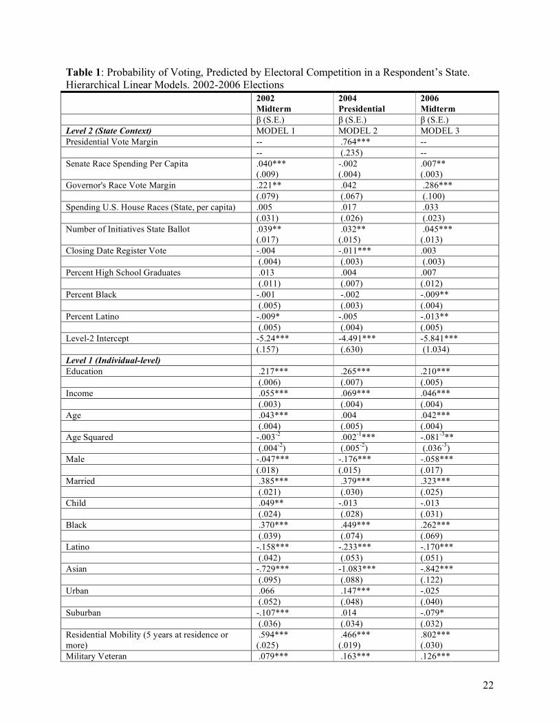
campaign activity in a respondent’s state. In Table 1, our measures of the mobilizing effects of

state-level electoral context include vote margin in presidential elections (1-vote margin between

the top 2 candidates) and gubernatorial races (1-vote margin).9 Higher values indicate a more

competitive election.10 We also model the effects of U.S. Senate and U.S. House spending per-

capita in a state for each of the three elections,11 and the number of ballot initiatives. Table 2

models turnout in 2004 with direct measures of campaign activity, including presidential

campaign visits to a states, the number of presidential television advertisements, presidential

television spending per capita in a state, and per capita campaign spending on ballot initiatives.12

Presidential campaign activity measures are highly correlated with one another and with

presidential vote margin and are thus modeled separately. We also include per capita total

spending (in $10,000s) in U.S. House races in a respondent’s state to represent campaign

activity.13 The CPS does not include county or zip code geographic identifiers, so we cannot

match respondents to their congressional district. Tests using the CCES data assess the effects of

district-level spending in House races.

The level 2 component of the model also includes voter registration closing date

measured by the number of days before an election needed to register to vote, ranging from 0 to

30 days prior. We expect residence in a state with more restrictive closing dates reduces the

10

probability of voting (Wolfinger and Rosenstone 1980). To account for the possibility that state

socioeconomic context affects individual propensity to participate (Hill and Leighley 1999;

1994), we include measures of the percent high school graduates, Latino, African American.

Individual Variables (Level 1)

Existing research suggests several individual-level demographic variables are necessary

controls (see appendix for descriptions of variable coding). We expect those with higher status

occupations, higher education, wealth and age,14 respectively, will be more likely to vote, other

things being equal. The CPS includes detailed measures of occupational status; we use the

industry and occupation job categories to represent a respondent’s primary occupation.15 As an

additional control, we include variables measuring whether the respondent was a government

employee as we expect government workers to have an increase probability of voting.16 Our

models include a binary variable measuring military veteran, and residential mobility is also

accounted for (Squire, Wolfinger and Glass 1987). A binary variable measures gender, with

males coded 1, as women may have higher turnout rates than men (Leighley and Nagler 1992).

CPS data include large samples of minority groups and binary variables are used to control for

ethnicity/race,17 marriage, school age children, as well as rural, suburban or urban places of

residence.18

CPS Multilevel Models

As noted, MLM is used to analyze the probability that a person reported voting in the

2002, 2004 and 2006 elections.19 Written as a population-average model, the level 2 equation

acts as the intercept for the level 1 equation; we allow each state to have its own intercept and we

allow the slopes for individual level education and age to vary by state.

Logit (PYij) = γ0+ β01 (Income) + β02 (Education) + β03 (Age) + β04 (Age Squared) +β05 (Male) + β06 (African-American) + β07 (Latino) + β08 (Asian-American) + β09 (Married) + β010 (Children) +β011 (Governor worker) +β012

(Military Veteran) + β013 (Residential Mobility) + β014 (Urban Resident) + β015 (Suburban) +β016 (Management) +

11

β017 (Professional) + β018 (Service) +β019 (Sales) + β020 (Secretarial) +β021 (Farming) +β022 (Transportation) +εu1(Age) + εu2(Education) + ε γ0 = γ00 + β1 (State Presidential Race Margin) + β2 (Governor Race Margin) + β3 (Spending Senate Race)+β4

(Spending U.S. House Races) + β5 (Percent Uncontested U.S. House Races) + β6 (Number/Spending Ballot Initiatives) + β7 (Closing Date Voter Registration) + β8 (Educational Attainment) + β9 (Percent black) + β10

(Percent Latino) +ε

An advantage of multilevel data is the ability to investigate cross-level hypotheses or

multilevel interactions. In our case, we are interested in how exposure to competitive elections

affects voter turnout for people at different ages and at different levels of education. Our models

include two additional random effect components, denoted as εu1 and εu2 above, to model

interactive effects of age and education. We hypothesize the effects of age and education on the

probability of voting may vary, depending on levels of exposure to information associated with

competitive elections. We allow the covariates for individual-level age and education to vary

across the state contextual (level 2) variables. These random effects interact age and education

with all the state electoral competition variables simultaneously. We thus avoid collinearity

problems that can be induced by multiple interaction terms.20 We also estimate cross-level

interactions, directly interacting the education and age of the respondent with campaign spending.

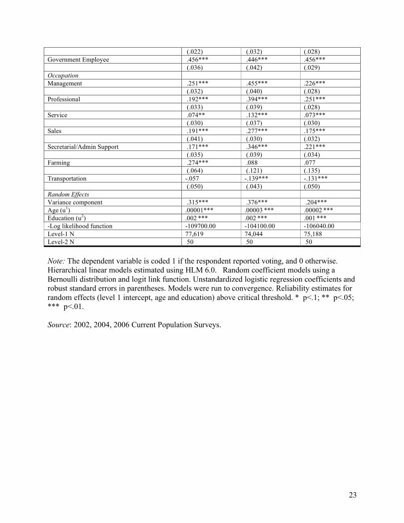
Table 1 presents evidence that exposure to competitive elections of all sorts increases the

probability of voting at the individual level. The effects of closer gubernatorial and U.S. Senate

races, as well as having ballot initiatives, both appear most pronounced at increasing turnout in

midterm elections. This makes sense given that the stimulus of presidential elections may swap

the mobilizing effects of down-ticket races in presidential years. While presidential years have

higher aggregrate mobilizing effects, we also see state-level presidential electoral competition

affects turnout in the presidential contest. Residing in a state with more ballot initiatives

increased the probability of voting in all years - this result holds even when the analysis is

constrained to only those states having ballot initiatives. (not shown).

12

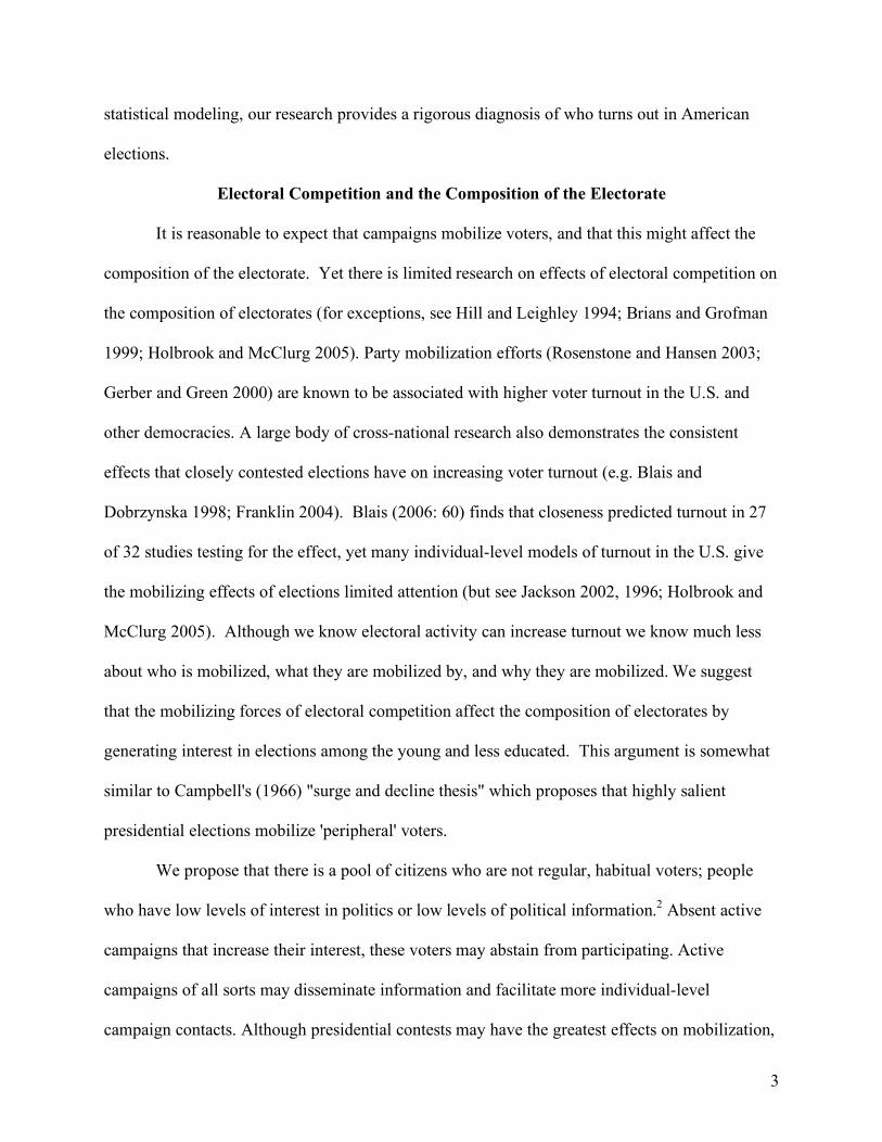
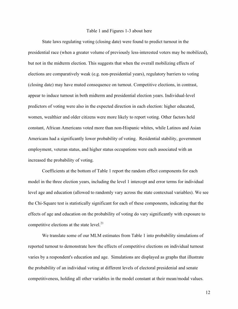
Table 1 and Figures 1-3 about here

State laws regulating voting (closing date) were found to predict turnout in the

presidential race (when a greater volume of previously less-interested voters may be mobilized),

but not in the midterm election. This suggests that when the overall mobilizing effects of

elections are comparatively weak (e.g. non-presidential years), regulatory barriers to voting

(closing date) may have muted consequence on turnout. Competitive elections, in contrast,

appear to induce turnout in both midterm and presidential election years. Individual-level

predictors of voting were also in the expected direction in each election: higher educated,

women, wealthier and older citizens were more likely to report voting. Other factors held

constant, African Americans voted more than non-Hispanic whites, while Latinos and Asian

Americans had a significantly lower probability of voting. Residential stability, government

employment, veteran status, and higher status occupations were each associated with an

increased the probability of voting.

Coefficients at the bottom of Table 1 report the random effect components for each

model in the three election years, including the level 1 intercept and error terms for individual

level age and education (allowed to randomly vary across the state contextual variables). We see

the Chi-Square test is statistically significant for each of these components, indicating that the

effects of age and education on the probability of voting do vary significantly with exposure to

competitive elections at the state level.21

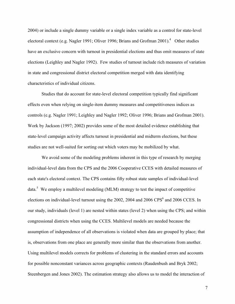
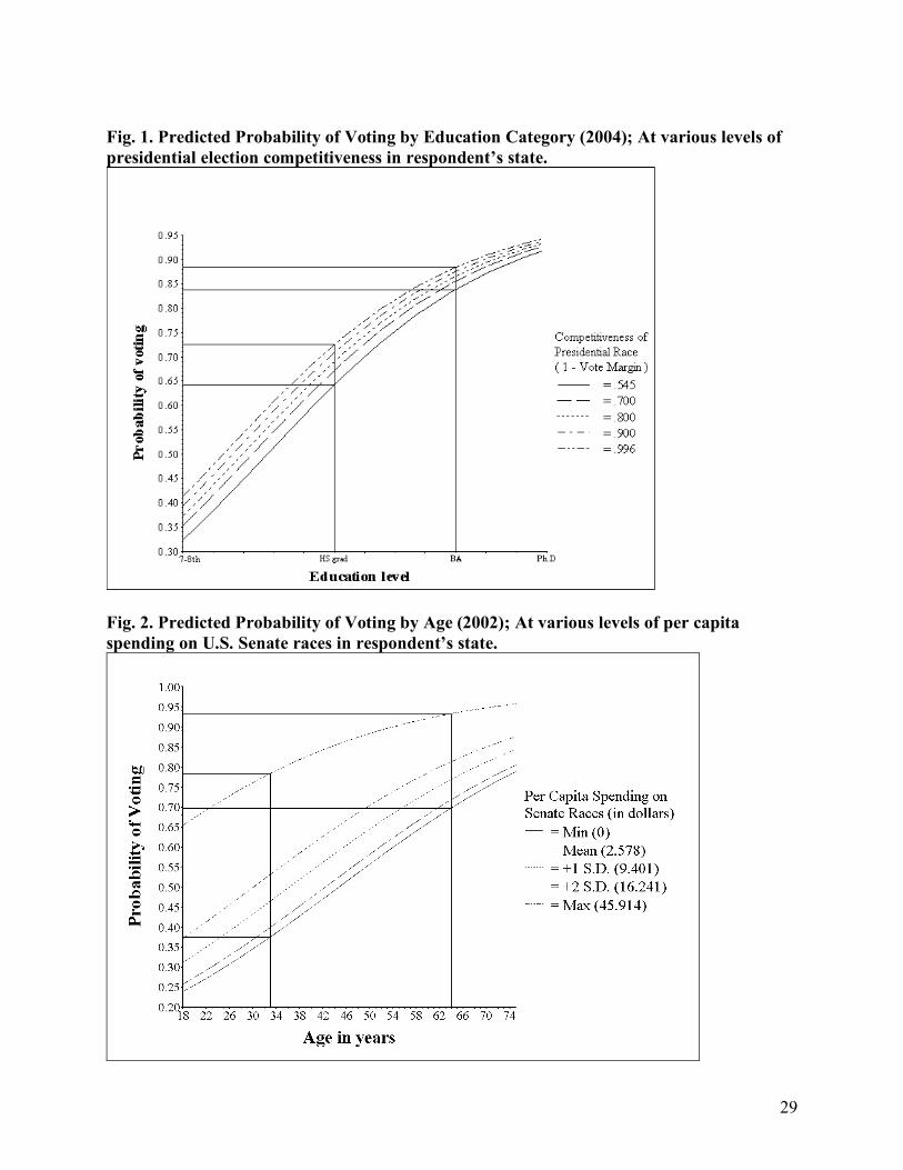
We translate some of our MLM estimates from Table 1 into probability simulations of

reported turnout to demonstrate how the effects of competitive elections on individual turnout

varies by a respondent's education and age. Simulations are displayed as graphs that illustrate

the probability of an individual voting at different levels of electoral presidenial and senate

competitiveness, holding all other variables in the model constant at their mean/modal values.

13

Figure 1 illustrates the probability that individuals with different levels of education reported

voting in 2004, predicted across state levels of presidential competitiveness. The figure

illustrates that residence in a state where the presidential race was more competitive had a greater

effect on turnout for people with less education than people with a college degree. Another

simulation (not reported) shows a similar effect for age: living in a competitive presidential state

had a disproportionate effect on turnout among younger voters. The capacity for a competitive

election context to change a marginal non-voter into a marginal voter can also be seen in Figure

1. Someone with a 10th Grade education residing in the least competitive presidential state in

2004 had a .46 estimated probability of reporting she voted, compared to a .55 probability for an

identical respondent in the most competitive state; a .09 difference.

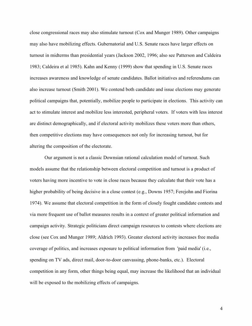
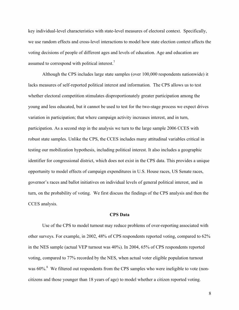
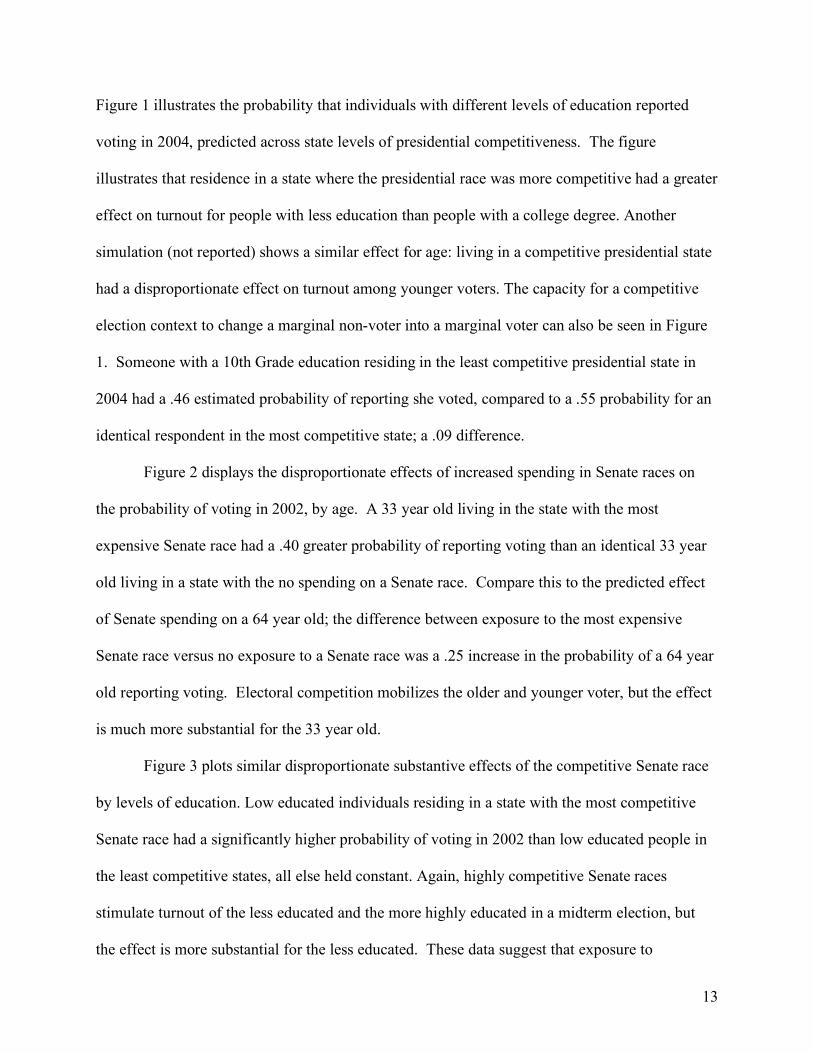
Figure 2 displays the disproportionate effects of increased spending in Senate races on

the probability of voting in 2002, by age. A 33 year old living in the state with the most

expensive Senate race had a .40 greater probability of reporting voting than an identical 33 year

old living in a state with the no spending on a Senate race. Compare this to the predicted effect

of Senate spending on a 64 year old; the difference between exposure to the most expensive

Senate race versus no exposure to a Senate race was a .25 increase in the probability of a 64 year

old reporting voting. Electoral competition mobilizes the older and younger voter, but the effect

is much more substantial for the 33 year old.

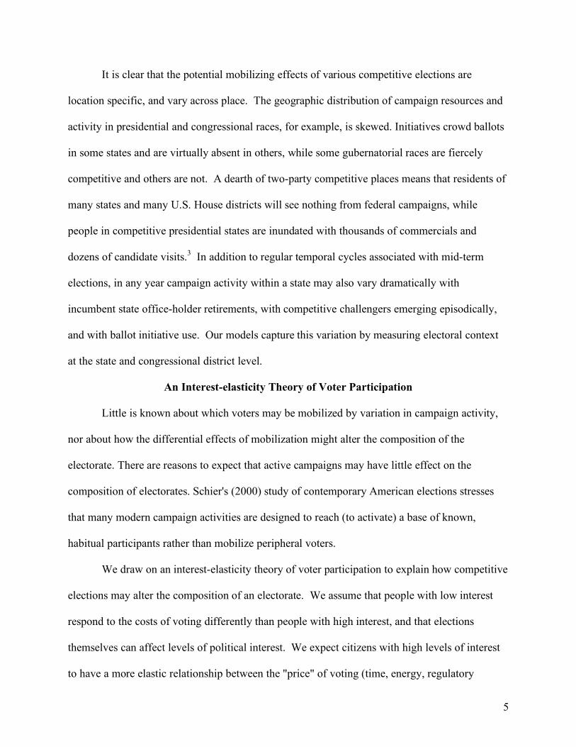
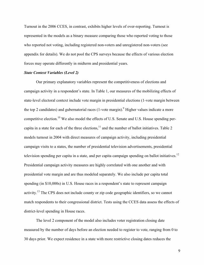
Figure 3 plots similar disproportionate substantive effects of the competitive Senate race

by levels of education. Low educated individuals residing in a state with the most competitive

Senate race had a significantly higher probability of voting in 2002 than low educated people in

the least competitive states, all else held constant. Again, highly competitive Senate races

stimulate turnout of the less educated and the more highly educated in a midterm election, but

the effect is more substantial for the less educated. These data suggest that exposure to

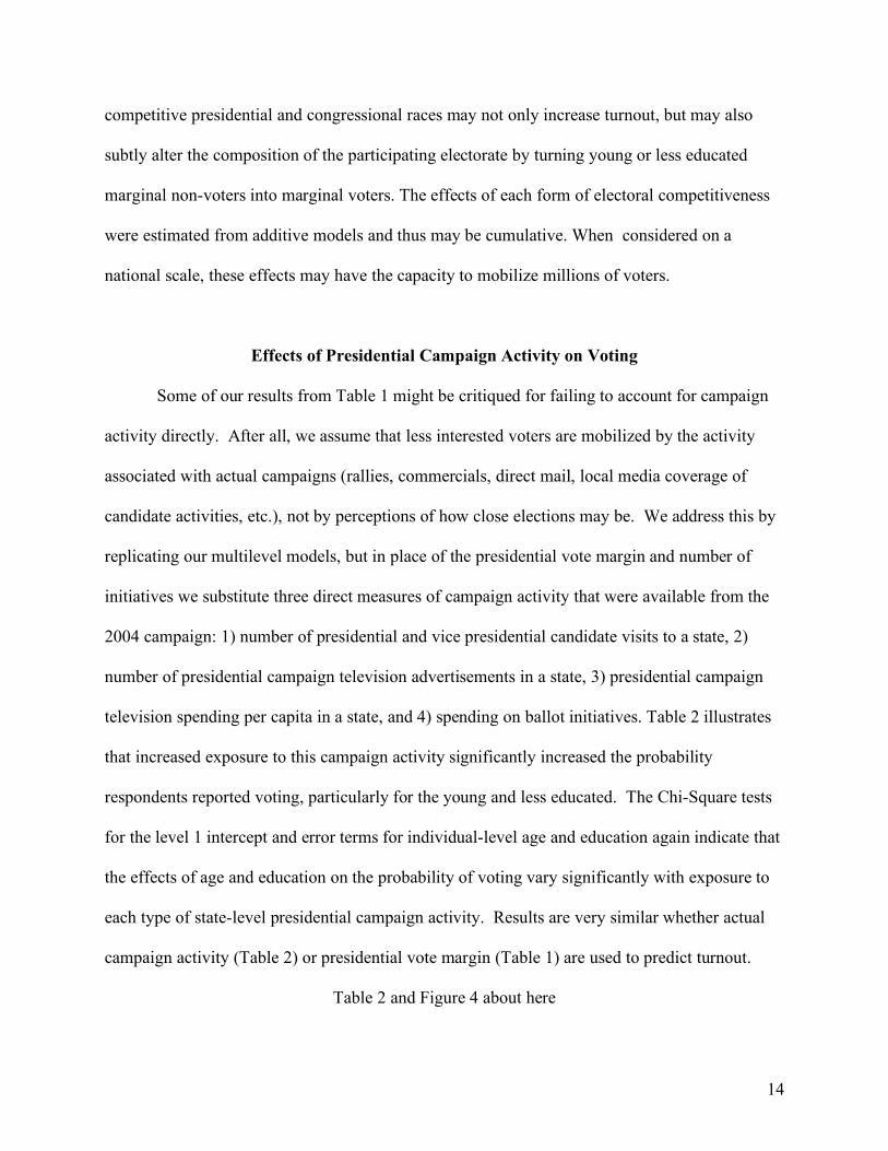
14

competitive presidential and congressional races may not only increase turnout, but may also

subtly alter the composition of the participating electorate by turning young or less educated

marginal non-voters into marginal voters. The effects of each form of electoral competitiveness

were estimated from additive models and thus may be cumulative. When considered on a

national scale, these effects may have the capacity to mobilize millions of voters.

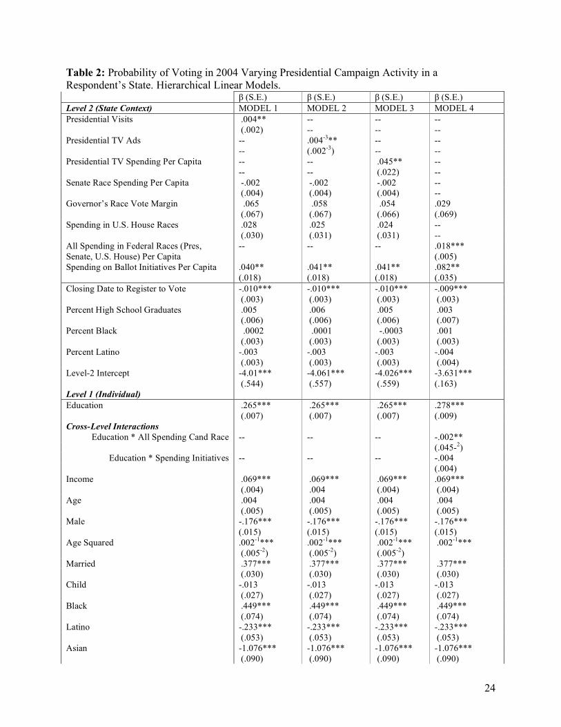
Effects of Presidential Campaign Activity on Voting

Some of our results from Table 1 might be critiqued for failing to account for campaign

activity directly. After all, we assume that less interested voters are mobilized by the activity

associated with actual campaigns (rallies, commercials, direct mail, local media coverage of

candidate activities, etc.), not by perceptions of how close elections may be. We address this by

replicating our multilevel models, but in place of the presidential vote margin and number of

initiatives we substitute three direct measures of campaign activity that were available from the

2004 campaign: 1) number of presidential and vice presidential candidate visits to a state, 2)

number of presidential campaign television advertisements in a state, 3) presidential campaign

television spending per capita in a state, and 4) spending on ballot initiatives. Table 2 illustrates

that increased exposure to this campaign activity significantly increased the probability

respondents reported voting, particularly for the young and less educated. The Chi-Square tests

for the level 1 intercept and error terms for individual-level age and education again indicate that

the effects of age and education on the probability of voting vary significantly with exposure to

each type of state-level presidential campaign activity. Results are very similar whether actual

campaign activity (Table 2) or presidential vote margin (Table 1) are used to predict turnout.

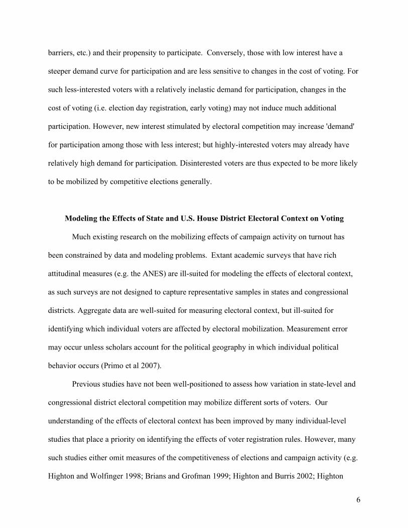
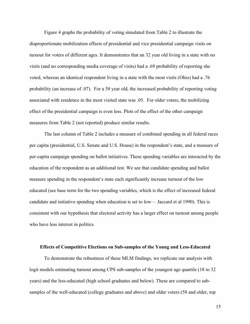
Table 2 and Figure 4 about here

15

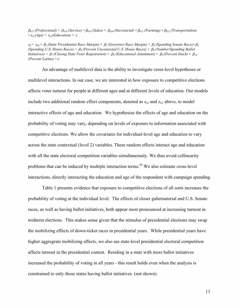
Figure 4 graphs the probability of voting simulated from Table 2 to illustrate the

disproportionate mobilization effects of presidential and vice presidential campaign visits on

turnout for voters of different ages. It demonstrates that an 32 year old living in a state with no

visits (and no corresponding media coverage of visits) had a .69 probability of reporting she

voted, whereas an identical respondent living in a state with the most visits (Ohio) had a .76

probability (an increase of .07). For a 58 year old, the increased probability of reporting voting

associated with residence in the most visited state was .05. For older voters, the mobilizing

effect of the presidential campaign is even less. Plots of the effect of the other campaign

measures from Table 2 (not reported) produce similar results.

The last column of Table 2 includes a measure of combined spending in all federal races

per capita (presidential, U.S. Senate and U.S. House) in the respondent’s state, and a measure of

per-capita campaign spending on ballot initiatives. These spending variables are interacted by the

education of the respondent as an additional test. We see that candidate spending and ballot

measure spending in the respondent’s state each significantly increase turnout of the low

educated (see base term for the two spending variables, which is the effect of increased federal

candidate and initiative spending when education is set to low— Jaccard et al 1990). This is

consistent with our hypothesis that electoral activity has a larger effect on turnout among people

who have less interest in politics.

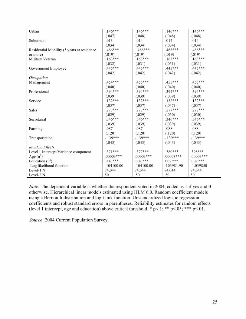
Effects of Competitive Elections on Sub-samples of the Young and Less-Educated

To demonstrate the robustness of these MLM findings, we replicate our analysis with

logit models estimating turnout among CPS sub-samples of the youngest age quartile (18 to 32

years) and the less-educated (high school graduates and below). These are compared to sub-

samples of the well-educated (college graduates and above) and older voters (58 and older, top

16

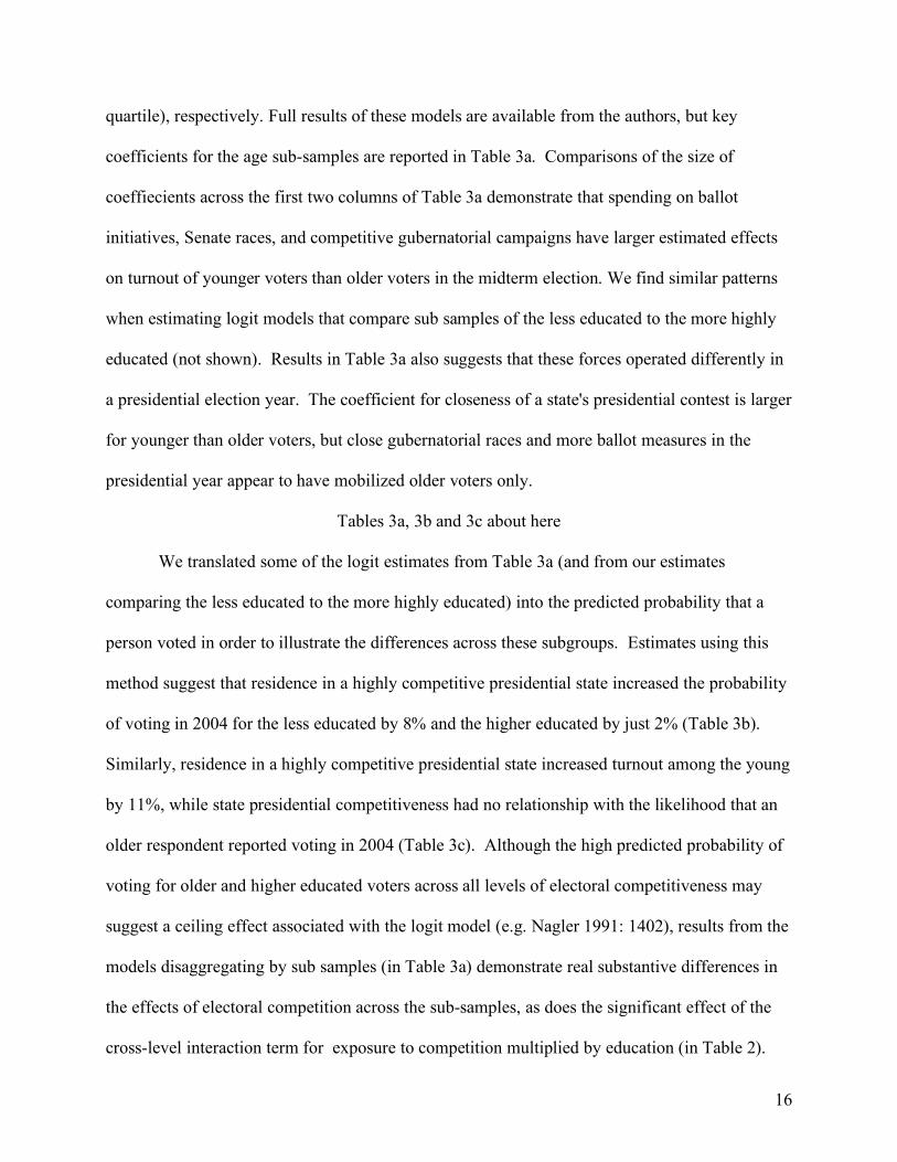
quartile), respectively. Full results of these models are available from the authors, but key

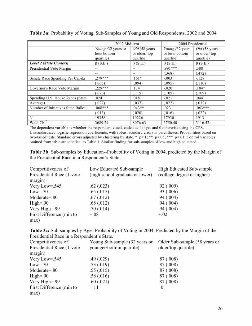
coefficients for the age sub-samples are reported in Table 3a. Comparisons of the size of

coeffiecients across the first two columns of Table 3a demonstrate that spending on ballot

initiatives, Senate races, and competitive gubernatorial campaigns have larger estimated effects

on turnout of younger voters than older voters in the midterm election. We find similar patterns

when estimating logit models that compare sub samples of the less educated to the more highly

educated (not shown). Results in Table 3a also suggests that these forces operated differently in

a presidential election year. The coefficient for closeness of a state's presidential contest is larger

for younger than older voters, but close gubernatorial races and more ballot measures in the

presidential year appear to have mobilized older voters only.

Tables 3a, 3b and 3c about here

We translated some of the logit estimates from Table 3a (and from our estimates

comparing the less educated to the more highly educated) into the predicted probability that a

person voted in order to illustrate the differences across these subgroups. Estimates using this

method suggest that residence in a highly competitive presidential state increased the probability

of voting in 2004 for the less educated by 8% and the higher educated by just 2% (Table 3b).

Similarly, residence in a highly competitive presidential state increased turnout among the young

by 11%, while state presidential competitiveness had no relationship with the likelihood that an

older respondent reported voting in 2004 (Table 3c). Although the high predicted probability of

voting for older and higher educated voters across all levels of electoral competitiveness may

suggest a ceiling effect associated with the logit model (e.g. Nagler 1991: 1402), results from the

models disaggregating by sub samples (in Table 3a) demonstrate real substantive differences in

the effects of electoral competition across the sub-samples, as does the significant effect of the

cross-level interaction term for exposure to competition multiplied by education (in Table 2).

17

In short, multiple modes of estimation here demostrate that electoral competition has a

disporportionate effect on mobilizing the young and less educated, a result consistent with our

assumtion that competition stimultates interest, which stimulates participation. But there is a

rival hypothesis. Key (1949) proposes that close elections may increase the incentives that

parties have to appeal to society's "have nots;" this suggests that electoral competition may

mobilize less affluent voters. We replicated our MLM models and simulations to for this

(available from authors). Rather than allowing age and education to interact with the effects of

elections, we allowed the respondent's income to interact with exposure to electoral competition.

We found no evidence that competitive elections mobilized turnout of low-income citizens more

or less relative to higher income citizens. This result is consistent with our theory grounded in

political interest - a theory that offers a mechanism to explain how competitive elections alter the

composition of electorates by generating interest among the young and less educated; rather than

by mobilizing voters with class-based appeals. As noted above, the CPS lacks direct measures of

political interest. We now turn to CCES data to address these shortcomings.

Electoral Competition, Political Interest and Turnout: CCES Data

Our theory suggests a two-stage process, where electoral competition increases interest in

politics, which in turns affects participation. The 2006 CCES allows us to model this process, as

it included identifiers linking respondents to their House districts and it included questions

asking about political interest and turnout.22 We merged state and congressional district-level

measures of electoral competition onto these CCES data to estimate a two-stage model, where

interest is our primary dependent variable in the first stage, and turnout is the dependent variable

in the second stage. In the second stage estimates, turnout is predicted with an instrumental

variable formed with the component of interest predicted by district-level US House race

18

campaign spending and other measures of electoral activity included in the first stage prediction

of interest. Interest is measured with responses to the question, “How interested are you in

politics and current affairs?” Response are coded as 1 for those “very much interested” and 0 if

the respondent said they were somewhat or not interested in politics. Turnout was coded 1 if the

respondent reported voting and 0 for not voting.

In the first stage, political interest is predicted by exposure to competitive elections and

other control variables. We measure 2006 campaign spending in the respondent’s U.S. House

district with raw data from the Federal Election Commission (FEC),23 since congressional

districts have comparable populations. We also measure total spending per capita on ballot

initiatives and referendums in the respondent’s state in 2006.24 Spending in U.S. Senate races is

again measured per capita. The models include standard demographic and ideology controls

matching as best as possible the CPS models. Models are estimated with logistic regression with

standard errors by clustered by congressional district.25

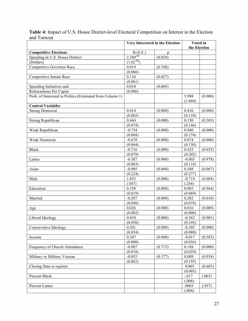
Table 4

Results in Table 4 demonstrate that individuals residing in US House districts with

greater spending were significantly more likely to report being very interested in politics.

Residence in a states with competitive US Senate races, and residence in states with greater

spending on ballot initiatives were also associated with a greater likelihood of being interested in

politics in 2006. This provides direct evidence that electoral competition increases political

interest. Most importantly, when we replicate the estimates in Table 4 across sub-samples that

compare younger voters to older voters, and less educated voters to higher educated voters (not

shown), we find the effects of spending on interest more pronounced among the young, and the

less educated. None of the measures of electoral competition increased interest among the high-

19

educated subsample. Column 2 in Table 4 demonstrates that interest stimulated by campaign

activity (estimated from Column 1) increases the likelihood of voting.

Discussion

Taken together, the sum of our results offer strong evidence that competitive elections

affect the composition of electorates. Competition mobilizes younger and less educated voters

more than others by stimulating interest in politics. Although it is difficult to generalize across

time from the data assessed here, our results suggest electoral competition affects who votes

across place, and over time. In presidential years, presidential campaigns may change a younger

or less-educated voter from a marginal non-voter into a marginal voter in highly competitive

states. Although relatively high levels of interest associated with presidential elections would

suggest a limit to how much competition might shape the electorate, our theory and results

suggest that when interest in a presidential election rises, turnout may increase disproportionately

among those previously less interested – the younger and less educated.

Although we do find that other forms of electoral competition stimulate interest and

disproportionately boost turnout of the young and less educated in midterm years, these results

are noteworthy since relatively few US House races are competitive in any given year and only

one-third of US Senate races can be competitive. The lack of a high-stimulus presidential

contest at the midterm, and a dearth of competitive congressional contests correspond with less

interest in politics and less turnout of the young and less educated at midterm elections. We

suggest this explains something we observe in the CPS: In 2002 and 2006, the average age of a

voter was 52. In 2004 the average voter was 49. The electorates were different because the

midterm contests were less interesting, and this muted participation of younger voters.

This is consistent with Schattschneider’s (1960) concern that low political participation is

one of the primary failures of American politics because it may produce a bias between the

20

general population and those who are actually represented. We have offered a theory of turnout,

grounded in political interest, to explain how active campaigns increase turnout

disproportionately among people with lower levels of political interest. Our contribution to the

understanding of voter turnout is to provide theoretical and empirical support for the idea that

competitive elections (and non competitive elections) do not have neutral effects on the

composition of an electorate. Electoral competition tends to increase turnout generally, but it can

also have a greater propensity to mobilize voters in groups known to have lower levels of

political interest: the young, and the less-educated. Active political campaigns that accompany

competitive elections may thus alter the composition of the electorate and reduce age and

education biases.

We illustrate how the effects of the electoral context a citizen resides in - namely,

exposure to competitive forces that stimulate political interest and mobilize voters - should be

seen as variable across time and place. In any given place, at any point in time, a unique set of

elections may stimulate a voter’s interest: state legislative races, contests for statewide office,

ballot measures, congressional races, and presidential elections. The more competitive these are,

the more likely it is that people less-interested in politics will vote. We suggest that the effects of

simultaneous exposure to multiple competitive elections may be cumulative. The relatively large

mobilizing effects of presidential elections on the young and less educated may mute the effects

of other contests in presidential years, but our results suggest there is substantial room for other

contests to mobilize these voters during midterms.

This study has implications for broader discussions about turnout. Our results illustrate

that laws placing barriers on voting are only part of the story about why so many people fail to

vote. Increased convenience of voting may have modest effects on turnout and on mitigating

existing bias in who participates (Fitzgerald 2005; Berinsky 2005). Barriers to voting declined

21

substantially after 1960, yet turnout (with the exceptions of the 2004 and 2008 presidential

contests) was consistently lower after the 1960s. Incumbent advantages and the geographic

distributions of partisans may have reduced the scope of exposure to competitive elections in the

U.S. since then. There were fewer competitive U.S. House races by 2000, and the geography of

U.S. presidential elections also changed substantially. In 1960 and 1968, the eight most

populous states were highly competitive in presidential politics, with an average margin of 2.4%

(s.d. 2.2) and 3.4% (s.d. 1.7), respectively. By 2004 and 2008, the eight most populous U.S.

states had many of the least competitive in presidential contests, with an average margin of 8.7%

(6.6 s.d) and 15.2% (9.3 s.d), respectively. New York, California and Texas were among the

most competitive states in presidential elections in the 1960s; in 2004 and 2008 they were among

the least competitive.

We suggest election reforms that may increase competition such as legislative

redistricting, changes to campaign finance regimes, and even modified forms of proportional

representation, may increase turnout overall - especially among the young and low-educated.

We concur with Franklin's suggestion (2004:3) that "the idea that declining turnout is due largely

to 'something about citizens' runs counter to some very obvious facts." Low turnout may have as

much to do with the character of elections as with the character of citizens. People vote for

various reasons, with one important reason being interest generated by elections. Compared to 40

years ago, a greater proportion of Americans now reside in places where the electoral context is

likely to offer little mobilizing effects from presidential and congressional campaigns. We have

demonstrated the importance of such exposure, and suggest this may be one reason for lower

levels of turnout since the 1960s.

22

Table 1: Probability of Voting, Predicted by Electoral Competition in a Respondent’s State. Hierarchical Linear Models. 2002-2006 Elections 2002

Midterm 2004 Presidential

2006 Midterm

β (S.E.) β (S.E.) β (S.E.) Level 2 (State Context) MODEL 1 MODEL 2 MODEL 3 Presidential Vote Margin -- .764*** -- -- (.235) -- Senate Race Spending Per Capita .040***

(.009) -.002 (.004)

.007** (.003)

Governor's Race Vote Margin .221** .042 .286*** (.079) (.067) (.100) Spending U.S. House Races (State, per capita) .005 .017 .033 (.031) (.026) (.023) Number of Initiatives State Ballot .039**

(.017) .032** (.015)

.045*** (.013)

Closing Date Register Vote -.004 -.011*** .003 (.004) (.003) (.003) Percent High School Graduates .013 .004 .007 (.011) (.007) (.012) Percent Black -.001 -.002 -.009** (.005) (.003) (.004) Percent Latino -.009* -.005 -.013** (.005) (.004) (.005) Level-2 Intercept -5.24*** -4.491*** -5.841*** (.157) (.630) (1.034) Level 1 (Individual-level) Education .217*** .265*** .210*** (.006) (.007) (.005) Income .055*** .069*** .046*** (.003) (.004) (.004) Age .043*** .004 .042*** (.004) (.005) (.004) Age Squared -.003-2 .002-1*** -.081-3** (.004-2) (.005-2) (.036-3) Male -.047*** -.176*** -.058*** (.018) (.015) (.017) Married .385*** .379*** .323*** (.021) (.030) (.025) Child .049** -.013 -.013 (.024) (.028) (.031) Black .370*** .449*** .262*** (.039) (.074) (.069) Latino -.158*** -.233*** -.170*** (.042) (.053) (.051) Asian -.729*** -1.083*** -.842*** (.095) (.088) (.122) Urban .066 .147*** -.025 (.052) (.048) (.040) Suburban -.107*** .014 -.079* (.036) (.034) (.032) Residential Mobility (5 years at residence or more)

.594*** (.025)

.466*** (.019)

.802*** (.030)

Military Veteran .079*** .163*** .126***

23

(.022) (.032) (.028) Government Employee .456*** .446*** .456*** (.036) (.042) (.029) Occupation Management .251*** .455*** .226*** (.032) (.040) (.028) Professional .192*** .394*** .251*** (.033) (.039) (.028) Service .074** .132*** .073*** (.030) (.037) (.030) Sales .191*** .277*** .175*** (.041) (.030) (.032) Secretarial/Admin Support .171*** .346*** .221*** (.035) (.039) (.034) Farming .274*** .088 .077 (.064) (.121) (.135) Transportation -.057 -.139*** -.131*** (.050) (.043) (.050) Random Effects Variance component .315*** .376*** .204*** Age (u1) .00001*** .00003 *** .00002 *** Education (u2) .002 *** .002 *** .001 *** -Log likelihood function -109700.00 -104100.00 -106040.00 Level-1 N 77,619 74,044 75,188 Level-2 N 50 50 50 Note: The dependent variable is coded 1 if the respondent reported voting, and 0 otherwise. Hierarchical linear models estimated using HLM 6.0. Random coefficient models using a Bernoulli distribution and logit link function. Unstandardized logistic regression coefficients and robust standard errors in parentheses. Models were run to convergence. Reliability estimates for random effects (level 1 intercept, age and education) above critical threshold. * p<.1; ** p<.05; *** p<.01. Source: 2002, 2004, 2006 Current Population Surveys.

24

Table 2: Probability of Voting in 2004 Varying Presidential Campaign Activity in a Respondent’s State. Hierarchical Linear Models. β (S.E.) β (S.E.) β (S.E.) β (S.E.) Level 2 (State Context) MODEL 1 MODEL 2 MODEL 3 MODEL 4 Presidential Visits .004** -- -- -- (.002) -- -- -- Presidential TV Ads -- .004-3** -- -- -- (.002-3) -- -- Presidential TV Spending Per Capita -- -- .045** -- -- -- (.022) -- Senate Race Spending Per Capita -.002 -.002 -.002 -- (.004) (.004) (.004) -- Governor’s Race Vote Margin .065 .058 .054 .029 (.067) (.067) (.066) (.069) Spending in U.S. House Races .028 .025 .024 -- (.030) (.031) (.031) -- All Spending in Federal Races (Pres, Senate, U.S. House) Per Capita

-- -- -- .018*** (.005)

Spending on Ballot Initiatives Per Capita .040** (.018)

.041** (.018)

.041** (.018)

.082** (.035)

Closing Date to Register to Vote -.010*** -.010*** -.010*** -.009*** (.003) (.003) (.003) (.003) Percent High School Graduates .005 .006 .005 .003 (.006) (.006) (.006) (.007) Percent Black .0002 .0001 -.0003 .001 (.003) (.003) (.003) (.003) Percent Latino -.003 -.003 -.003 -.004 (.003) (.003) (.003) (.004) Level-2 Intercept -4.01*** -4.061*** -4.026*** -3.631*** (.544) (.557) (.559) (.163) Level 1 (Individual) Education .265*** .265*** .265*** .278*** (.007) (.007) (.007) (.009) Cross-Level Interactions

Education * All Spending Cand Race -- -- -- -.002** (.045-2)

Education * Spending Initiatives -- -- -- -.004 (.004)

Income .069*** .069*** .069*** .069*** (.004) .004 (.004) (.004) Age .004 .004 .004 .004 (.005) (.005) (.005) (.005) Male -.176*** -.176*** -.176*** -.176*** (.015) (.015) (.015) (.015) Age Squared .002-1*** .002-1*** .002-1*** .002-1*** (.005-2) (.005-2) (.005-2) Married .377*** .377*** .377*** .377*** (.030) (.030) (.030) (.030) Child -.013 -.013 -.013 -.013 (.027) (.027) (.027) (.027) Black .449*** .449*** .449*** .449*** (.074) (.074) (.074) (.074) Latino -.233*** -.233*** -.233*** -.233*** (.053) (.053) (.053) (.053) Asian -1.076*** -1.076*** -1.076*** -1.076*** (.090) (.090) (.090) (.090)

25

Urban .146*** .146*** .146*** .146*** (.047) (.048) (.048) (.048) Suburban .013 .014 .014 .014 (.034) (.034) (.034) (.034) Residential Mobility (5 years at residence or more)

.466*** (.019)

.466*** (.019)

.466*** (.019)

.466*** (.019)

Military Veteran .163*** .163*** .163*** .163*** (.032) (.031) (.031) (.031) Government Employee .445*** .445*** .445*** .445*** (.042) (.042) (.042) (.042) Occupation Management .454*** .455*** .455*** .455*** (.040) (.040) (.040) (.040) Professional .394*** .394*** .394*** .394*** (.039) (.039) (.039) (.039) Service .132*** .132*** .132*** .132*** (.037) (.037) (.037) (.037) Sales .277*** .277*** .277*** .277*** (.029) (.029) (.030) (.030) Secretarial .346*** .346*** .346*** .346*** (.039) (.039) (.039) (.039) Farming .087 .087 .088 .088 (.120) (.120) (.120) (.120) Transportation -.139*** -.139*** -.139*** -.139*** (.043) (.043) (.043) (.043) Random Effects Level 1 Intercept/Variance component .371*** .377*** .380*** .398*** Age (u1) .00003*** .00003*** .00003*** .00003*** Education (u2) .002 *** .002 *** .002 *** .002 *** -Log likelihood function -104100.00 -104100.00 -103981.90 -1.039850 Level-1 N 74,044 74,044 74,044 74,044 Level-2 N 50 50 50 50 Note: The dependent variable is whether the respondent voted in 2004, coded as 1 if yes and 0 otherwise. Hierarchical linear models estimated using HLM 6.0. Random coefficient models using a Bernoulli distribution and logit link function. Unstandardized logistic regression coefficients and robust standard errors in parentheses. Reliability estimates for random effects (level 1 intercept, age and education) above critical threshold. * p<.1; ** p<.05; *** p<.01. Source: 2004 Current Population Survey.

26

Table 3a: Probability of Voting, Sub-Samples of Young and Old Respondents, 2002 and 2004 2002 Midterm 2004 Presidential Young (32 years or

less/ bottom quartile)

Old (58 years or older/ top quartile)

Young (32 years or less/ bottom quartile)

Old (58 years or older/ top quartile)

Level 2 (State Context) β (S.E.) β (S.E.) β (S.E.) β (S.E.) Presidential Vote Margin -- -- .991*** .388 -- -- (.368) (.472) Senate Race Spending Per Capita .279*** .161* -.003 -.128 (.065) (.094) (.095) (.110) Governor's Race Vote Margin .229*** .134 -.020 .184* (.076) (.115) (.105) (.109) Spending U.S. House Races (State .024 .018 -.021 .044 Average) (.027) (.037) (.022) (.032) Number of Initiatives State Ballot .068*** .043** .023 .063*** (.013) (.020) (.016) (.022) N 19358 19226 17930 1913 Wald Chi2 3689.24 8076.63 3750.40 3116.52 The dependent variable is whether the respondent voted, coded as 1 if yes and 0 otherwise using the CPS. Unstandardized logistic regression coefficients, with robust standard errors in parentheses. Probabilities based on two-tailed tests. Standard errors adjusted by clustering by state. * p<.1; ** p<.05; *** p<.01. Control variables omitted from table are identical to Table 1. Similar finding for sub-samples of low and high educated. Table 3b: Sub-samples by Education--Probability of Voting in 2004, predicted by the Margin of the Presidential Race in a Respondent’s State. Competitiveness of Presidential Race (1-vote margin)

Low Educated Sub-sample (high school graduate or lower)

High Educated Sub-sample (college degree or higher)

Very Low=.545 .62 (.023) .92 (.009) Low=.70 .65 (.015) .93 (.006) Moderate=.80 .67 (.012) .94 (.004) High=.90 .68 (.012) .94 (.004) Very High=.99 .70 (.014) .94 (.004) First Difference (min to max)

+.08 +.02

Table 3c: Sub-samples by Age--Probability of Voting in 2004, Predicted by the Margin of the Presidential Race in a Respondent’s State. Competitiveness of Presidential Race (1-vote margin)

Young Sub-sample (32 years or younger/bottom quartile)

Older Sub-sample (58 years or older/top quartile)

Very Low=.545 .49 (.029) .87 (.008) Low=.70 .53 (.019) .87 (.008) Moderate=.80 .55 (.015) .87 (.008) High=.90 .58 (.016) .87 (.008) Very High=.99 .60 (.021) .87 (.008) First Difference (min to max)

+.11 0

27

Table 4: Impact of U.S. House District-level Electoral Competition on Interest in the Election and Turnout Very Interested in the Election Voted in

the Election Competitive Elections Β (S.E.) p Spending in U.S. House District 2.380-08 (0.020) (Dollars) (1.02-08) Competitive Governor Race 0.019 (0.768) (0.066) Competitive Senate Race 0.136 (0.027) (0.061) Spending Initiatives and 0.018 (0.005) Referendums Per Capita (0.006) Prob. of Interested in Politics (Estimated from Column 1) 5.988

(1.044) (0.000)

Control Variables Strong Democrat 0.414 (0.000) 0.436 (0.000) (0.065) (0.110) Strong Republican 0.444 (0.000) 0.150 (0.305) (0.074) (0.146) Weak Republican -0.754 (0.000) 0.940 (0.000) (0.068) (0.174) Weak Democrat -0.678 (0.000) 0.874 (0.000) (0.064) (0.150) Black -0.716 (0.000) 0.425 (0.035) (0.079) (0.202) Latino -0.387 (0.000) -0.003 (0.978) (0.083) (0.116) Asian -0.905 (0.000) 0.508 (0.067) (0.224) (0.277) Male 1.053 (0.000) -0.714 (0.004) (.047) (.244) Education 0.358 (0.000) 0.003 (0.964) (0.019) (0.069) Married -0.207 (0.000) 0.202 (0.010) (0.048) (0.078) Age 0.026 (0.000) 0.016 (0.009) (0.002) (0.006) Liberal Ideology 0.410 (0.000) -0.362 (0.001) (0.058) (0.105) Conservative Ideology 0.301 (0.000) -0.305 (0.000) (0.054) (0.080) Income 0.107 (0.000) -0.017 (0.503) (0.008) (0.026) Frequency of Church Attendance -0.007 (0.715) 0.188 (0.000) (0.018) (0.029) Military or Military Veteran -0.055 (0.377) 0.008 (0.934) (0.062) (0.195) Closing Date to register 0.003 (0.605) (0.005) Percent Black -.017 (.003) (.006) Percent Latino .0003 (.937) (.004)

28

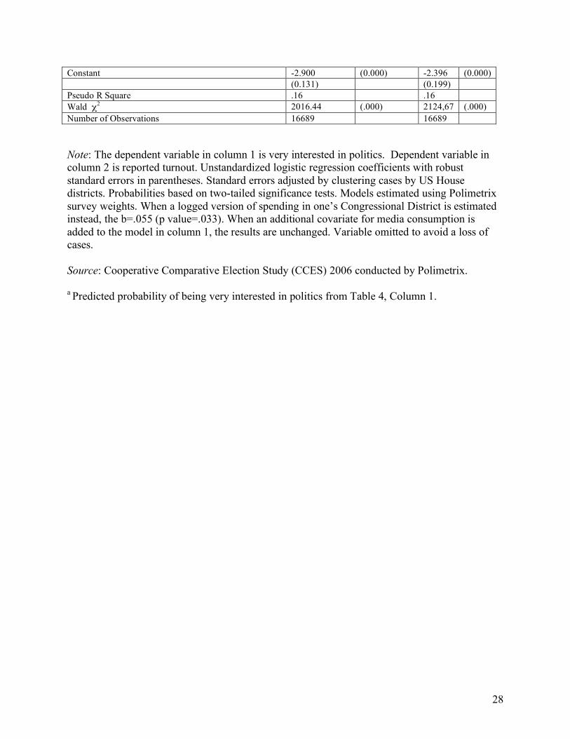
Constant -2.900 (0.000) -2.396 (0.000) (0.131) (0.199) Pseudo R Square .16 .16 Wald χ2 2016.44 (.000) 2124,67 (.000) Number of Observations 16689 16689 Note: The dependent variable in column 1 is very interested in politics. Dependent variable in column 2 is reported turnout. Unstandardized logistic regression coefficients with robust standard errors in parentheses. Standard errors adjusted by clustering cases by US House districts. Probabilities based on two-tailed significance tests. Models estimated using Polimetrix survey weights. When a logged version of spending in one’s Congressional District is estimated instead, the b=.055 (p value=.033). When an additional covariate for media consumption is added to the model in column 1, the results are unchanged. Variable omitted to avoid a loss of cases. Source: Cooperative Comparative Election Study (CCES) 2006 conducted by Polimetrix. a Predicted probability of being very interested in politics from Table 4, Column 1.

29

Fig. 1. Predicted Probability of Voting by Education Category (2004); At various levels of presidential election competitiveness in respondent’s state.

Fig. 2. Predicted Probability of Voting by Age (2002); At various levels of per capita spending on U.S. Senate races in respondent’s state.

30

Fig. 3 Predicted Probability of Voting by Education (2002); At various levels of per capita spending on U.S. Senate Races in respondent’s state.

Fig. 4. Predicted Probability of Voting by Age (2004); At various numbers of presidential candidate visits to respondent’s state.

31

References

Aldrich, John. 1993. “Rational Choice and Turnout.” American Journal of Political Science 37 (1):

246–78.

Berinsky, Adam. 2005. “The Perverse Consequences of Electoral Reform in the United States.”

American Politics Research 33: 471-491.

Blais, Andre. 2006. "What Affects Voter Turnout?" Annual Review of Political Science. 9:111-25.

Blais, Andre and A. Dobrzynska. 1998. "Turnout in Electoral Democracies." European Journal of

Political Research. 18:167-81

Brians, Craig and Bernard Grofman. 1999. "When Registration Barriers Fall, Who Votes? An

Empirical Test of a Rational Choice Model." Public Choice. 99-161-76,

Brians, Craig and Bernard Grofman. 2001. “Election Day Registration’s Effect on U.S. Voter

Turnout.” Social Science Quarterly 82 (1): 170-183.

Bryk, AS and SW Raudenbush. 2002. Hierarchical Linear Models: Applications and Data Analysis

Methods. Sage Publications.

Caldeira, Gregory A., Patterson, Samuel C., and Markko, Gregory A. 1985. “The Mobilization of

Voters.” Journal of Politics 47: 490–509.

Campbell, Angus. 1966. “Surge and Decline: A Study of Electoral Change.” In A. Campbell, P.E.

Converse, W.E. Miller and D.E. Stokes (Eds.) Elections and the Political Order. New York: Wiley.

Cox, Gary and M. C. Munger. 1989. Closeness, Expenditures and Turnout in the 1982 U.S. House

Elections” American Political Science Review. 83(1): 217-231.

Downs, Anthony. 1957. An Economic Theory of Democracy. New York: Harper & Row.

Ferejohn, John A., and Morris P. Fiorina. 1974. "The Paradox of Not Voting: A Decision Theoretic

Analysis." American Political Science Review 68: 525-546.

32

Fitzgerald, Mary. 2005. “Greater Convenience but not Greater Turnout: The Impact of Alternative

Voting Methods on Electoral Participation in the United States.” American Political

Research 33: 842-867.

Franklin, Mark N. 2004. Voter Turnout and the Dynamics of Electoral Competition in Established

Democracies Since 1945. Cambridge University Press.

Gerber, Alan S. and Green, Donald P. 2000. “The Effects of Canvassing, Telephone Calls, and

Direct Mail on Voter Turnout: A Field Experiment.” American Political Science Review 94:

653–663.

Green, Donald P. and Ian Shapiro. 1994. Pathologies of Rational Choice Theory. New Haven: Yale

University Press.

Highton, Benjamin. 1997. “Easy Registration and Voter Turnout.” Journal of Politics 59 (2): 565-575.

Highton, Benjamin. 2004. “Voter Registration and Turnout in the United States.” Perspectives on

Politics. 2(2):507-505.

Highton, Benjamin and A. Burris 2002. "New Perspectives on Latino Voter Turnout in the United

States. American Politics Research. 30:3:285 -306.

Highton, Benjamin and Raymond Wolfinger 1998. Estimating the Effects of the National Voter

Registration Act of 1993. Political Behavior. 20(2): 79-104.

Hill, Kim Quaile and Jan Leighley. 1994. "Mobilizing Institutions and Class Representation in U.S.

State Electorates. Political Research Quarterly. 47(1): 137-50.

Hill, Kim and Jan Leighley. 1999. “Racial Diversity, Voter Turnout, and Moblizing Institutions in

the United States.” American Politics Quarterly 27: 275-295.

Holbrook, Thomas and Scott McClurg. 2005. “The Mobilization of Core Supporters: Campaigns,

Turnout, and Electoral Composition in United States Presidential Elections.” American

33

Journal of Political Science 49 (4): 689-703.

Jackson, Robert A. 1996. “A Reassessment of Voter Mobilization.” Political Research Quarterly

49: 331– 349.

Jackson, Robert A. 1997. “The Mobilization of U.S. State Electorates in the 1998 and 1990

Elections.” Journal of Politics 59: 520-37.

Jackson, Robert A. 2002. "Gubernatorial and Senatorial Campaign Mobilization of Voters."

Political Research Quarterly. 55(4): 825-844.

Jaccard, James, Robert Turrisi, and Choi Wan. 1990. "Interactive Effects in Multiple Regression."

Sage Series on Quantitative Applications in Social Sciences, # 72. Newbury Park, CA: Sage.

Kahn, K.F. and P.J. Kenny. 1999. The Spectacle of U.S. Senate Campaigns. Princeton, NJ:

Princeton University Press.

Karp, Jeffrey A. and Susan A. Banducci. 2000. “Going postal: How All-Mail Elections Influence

Turnout.” Political Behavior 22: 223-239.

Key, V.O. 1949. Southern Politics in State and Nation. New York, NY: Knopf.

Leighley, Jan and Jonathan Nagler. 1992. “Individual and Systemic Influences on Turnout: Who

Votes?” Journal of Politics 54: 718-741.

McDonald, Michael and John Samples, eds. 2006. The Marketplace of Democracy: Electoral

Competition and American Politics. Washington, DC: Brookings Institute Press.

Nagler, Jonathan. 1991. “The Effect of Registration Laws and Education on U.S. Voter Turnout."

American Political Science Review 85:1393-1405.

Oliver, J. Eric. 1996. “The Effects of Eligibility Restrictions and Party Activity on Absentee Voting

and Overall Turnout.” American Journal of Political Science 40: 498-514.

Patterson, Samuel C. and Gregory Caldeira. 1983. “Getting Out the Vote: Participation in

34

Gubernatorial Elections.” American Political Science Review 77(3): 675-89.

Primo, David M., Matthew L. Jacobsmeier, and Jeffrey Milyo. 2007. “Estimating the Impact of

State Policies and Institutions with Mixed-Level Data,” State Politics and Policy Quarterly

7: 446-59.

Rosenstone, Steven and John Mark Hansen. 2003. Mobilization, Participation, and Democracy in

America. New York: Macmillan.

Schattschneider, E. E. 1960. The Semi-sovereign People. New York: Harcourt Brace.

Schier, Steven. 2000. By Invitation Only: The Rise of Exclusive Politics in the United States.

Pittsburgh: University of Pittsburgh Press.

Smith, Mark. 2001. “The Contingent Effects of Ballot Initiatives and Candidate Races on

Turnout.” American Journal of Political Science 45: 700-06.

Squire, Peverill, Raymond E. Wolfinger, David P. Glass. 1987. “Residential Mobility and Voter

Turnout. The American Political Science Review 81 (1): 45-66.

Steenbergen, Maro, and Bradford Jones. 2002. “Modeling Multilevel Data Structures.” American

Journal of Political Science 41(1): 218–37.

Wolfinger, Raymond, and Steven J. Rosenstone. 1980. Who Votes? New Haven: Yale University

Press.

Wolfinger, Robert, Benjamin Highton and M. Mullin. 2005. “How Postregistration Laws affect the

Turnout of Citizens Registered to Vote.” State Politics and Policy Quarterly 5: 1-23.

35

Appendix: Variable coding for Current Population Surveys

Voted / not voted: Following the CPS published reports, we code respondents indicating they did

not vote (question pes1) as non voters, as well refused, don’t know and no response.

Respondents reporting “yes” on question pes1 were coded as voters. In 2002 of 97,684 valid

respondents, 47,377 (48.5%) reported voting. In 2004 of 95,408 respondents, 62,328 reported

they voted. In the 2006 survey had 93, 331 respondents. Occupational categories include: 1)

management, business, and financial, 2) professional and related, 3) service, 4) sales and related,

5) office and administrative support, 6) farming, fishing, and forestry, 7) construction and

extraction, 8) installation, maintenance, and repair, 9) production, 10) transportation and material

moving, and 11) armed forces. Minor variations in these categories over the eights years of the

study. Residential Mobility: Respondents living at the same address for fives years or longer are

coded 1, and those less than five years 0. Military veteran (or currently in the military), coded 1

with non-veterans coded as 0. Education: 1=Less than 1st; 2=1st-3rd grade; 3= 5th-6th grade;

4=7th-8th grade; 5=9th grade; 6=10th; 7= 11th; 8=12th grade, no diploma; 9= high school grad-

diploma or equivalent; 10=some college, no degree; 11=associate degree-occupational/vocational;

12=Associated degree-academic program; 13=Bachelor’s degree; 14=Master’s degree (ma, ms,

meng, med, MSW); 15=Professional school degree (md, dds, dvm); 16=Doctorate degree (PhD,

EdD). Income categories: 1= less than 5k; 2=5k-7,499; 3=7,500-9,999; 4=10k-12499; 5=12500-

14999; 6=15k-19,999; 7=20k-24999; 8=25000-29999; 9=30000-34999; 10=35k-39,999; 11=40k-

49999; 12=50k-59999; 13=60k-74999; 14=75000 or more. In 2004 and 2006, categories also

included: 14=75k-99,999; 15=100k-149,999; 16=150k and over. Urban: From Geography-

MSA/central city status. All those who said “Central City” were coded 1; everyone else 0.

Change: in 2004, Central city status was called “Principal city.” Suburban: From Geography-

MSA/central city status. All those who said “Balance On MSA” =1; everyone else 0.

36

Endnotes

1 See Highton 1997 and Leighley and Nagler 1992 for early examples using multilevel measures.

2 As evidence, the 2004 National Post Election Study shows that 92% of respondents who

reported they voted said in the pre-election survey that they were "very interested" in following

the campaign. Only 8% of self-reported non voters said they were "very interested" the

campaign when asked in the pre-election survey.

3 See Center for Voting and Democracy study (2005) and McDonald and Samples (2006).

4 Nagler (1991) included a dummy for states with gubernatorial contests. Oliver included a

dummy for states with an "active" party. Brians and Grofman (2001) included an index of

competitiveness built from democratic presidential candidate's share of the two-party vote.

5 In 2004, for example, state sample sizes ranged from a high of 6007 California respondents and

4179 New York respondents to a low of 984 respondents from Missouri. Unlike many surveys,

the CPS includes robust samples from all fifty states, including Alaska (1316) and Hawaii

(1289). Similar state samples are found in the 2002 and 2006 CPS.

6 CPS November Voting Supplement conducted in 2002, 2004, 2006 by the U.S. Census Bureau.

7 For example, the 2004 American National Election Study (NES) shows that the 7 category NES

measure of education and the 3 category measure of interest in political campaigns have a strong

association (Chi Square 79.9, p. < .000. Thirty-five percent of respondents with a high school

degree reported being "very" interested, compared to 60% of those with a BA degree, and 76%

of those with an advanced degree. Voters younger than 32, likewise, were less interested (43%)

than voters over 32 (55%), Chi Square 17.5, p. < p. .000.

8 For voter eligible turnout (VEP) rates in the three elections see McDonald, Michael. United

States Election Project. Online: http://elections.gmu.edu/voter_turnout.htm.

37

9 The presidential margin raw data come from www.presidentelect.org; the data for gubernatorial

margin come from The Almanac of American Politics (various years).

10 For margin, the difference between the percent of votes for the winner and percent for the loser

are decimal 1-(%for winner-% for runner up).

11 Results are unchanged when models are estimated using Senate vote margin rather than per

capita Senate race spending. Available from authors.

12 Initiative spending data was only available for 2004. Data from National Conference of State

Legislatures (http://www.ncsl.org) and the Ballot Initiative Strategy Center (BISC).

13 This variable measures total U.S. House campaign expenditures for the entire state reported to

the FEC (by the campaign – it does not include PAC spending) divided by the 2000 population

of that state. Source: http://www.fec.gov/finance/disclosure/ftpsum.shtml.

14 To account for any nonlinear effects of declining participation among the oldest citizens, a

square term for age is also included.

15 A binary variable was created for each occupation, with production and construction as the

reference category.

16 Federal, state, and local government employee coded 1, with all others coded 0

17 Three binary variables represent whether the respondent is an African-American, Latino or

Asian or Pacific Islander (respectively), with white non-Hispanic as the reference group.

18 Because marriage and having children may increase community ties and political participation

(Putnam 2000) we include binary variables for married respondents and those with a child under

the age of 18 residing at home, respectively. Geography/location is measured with binary

variables for urban and suburban residents, with rural residents and those that did not identify

their location as the reference group.

38

19 We estimate hierarchical (multilevel) random coefficient models using a binominal Bernoulli

distribution and logit link function in HLM 6.0.

20 We estimate the models with random varying slope coefficients for age and education,

allowing these individual level factors to vary across all the second level variables measuring

electoral context. Random effects provide a natural way to model interactions between individual

level factors and state electoral context. Multiple cross-level interactions for age and education

and each form of electoral competition/campaign activity cause multicollinearity problems.

21 Because of the large number of explanatory variables, only one or two random effects can be

included, or else HLM will fail to converge (Bryk and Raudenbush 2002).

22 This sample is constructed using a technique called sample matching. The researchers create a

list of all U.S. consumers to generate a set of demographic characteristics that should be mirrored

in the survey sample. Then, using a matching algorithm, they select respondents who most

closely resemble the consumer data from a pool of opt-in participants. The sample is stratified to

ensure large samples within states. More information regarding sample matching is available at

http://web.mit.edu/polisci/portl/cces/material/sample_matching.pdf. These data were collected

over a three-month period from September to November of 2006 (Ansolabehere 2007).

23 Replications using the log of dollars spent produce similar findings.

24 Data is from www.followthemoney.org.

25 The results hold if the models are estimated by clustering by state instead of congressional

district, but are more robust by adjusting the standard errors for the smaller geographic unit. We

estimate the models using Huber-White robust standard errors and by weighting observations

using the Polimetrix survey weights.