Embed Size (px)
Citation preview

i
TOWARDS A DESIGN ENVIRONMENT FOR BUILDING-
INTEGRATED ENERGY SYSTEMS: THE INTEGRATION
OF ELECTRICAL POWER FLOW MODELLING WITH
BUILDING SIMULATION
Nicolas James Kelly B.Eng., M.Sc.
A thesis submitted for the
Degree of Doctor of Philosophy
Department of Mechanical Engineering
Energy Systems Research Unit
University of Strathclyde, Glasgow, UK.
October 1998

ii
to my family

iii
© The Copyright of this thesis belongs to the author under the terms of the United Kingdom
Copyright Acts as qualified by the University of Strathclyde Regulation 3.49. Due
acknowledgement must always be made to the use of any material contained in or derived from
this thesis.

iv
Table of Contents
Acknowledgements ................................................................................................................... x
Abstract.................................................................................................................................... xi
Chapter 1 - Buildings Energy and Environment ..................................................................... 1
1.1 Energy Use within Buildings............................................................................................1
1.1.1 Environmental Implications.......................................................................................2
1.1.2 Economic Implications ..............................................................................................3
1.2 The Means of Reducing Energy Consumption..................................................................4
1.2.1 Energy End-Use Reduction........................................................................................4
1.2.2 Reducing High-Grade Energy Usage .........................................................................5
1.2.3 Electrical Energy Displacement .................................................................................7
1.2.4 The Advantages of Building-Integrated Power Generation.........................................8
1.3 Designing for Building-Integrated Energy Systems ..........................................................9
1.3.1 Towards an Integrated Design Tool .........................................................................10
1.4 Objectives ......................................................................................................................10
1.5 Larger-Scale Energy Systems .........................................................................................12
1.6 Summary .......................................................................................................................12
1.7 References .....................................................................................................................13
Chapter 2 - Modelling the Building........................................................................................ 15
2.1 The ESP-r System..........................................................................................................15
2.2 Control Volumes............................................................................................................16
2.2.1 The Control Volume Applied to a Zone ...................................................................18
2.2.2 Application of a Mass Balance to the Fluid Volume.................................................23
2.2.3 Application of Energy Mass and Momentum Balances (CFD) .................................25
2.2.4 The Control Volume Applied to the Building Fabric................................................28
2.2.5 The Control Volume Applied to Plant Components..................................................35
2.3 Treatment and Solution of the Finite Volume Equation Sets ...........................................40
2.3.1 Zonal Energy Equations ..........................................................................................40
2.3.2 The Plant Energy Equations.....................................................................................45

v
2.3.3 Treatment of Time-Varying and Non-Linear Processes ............................................46
2.3.4 The Fluid Flow Equations........................................................................................47
2.4 Simultaneous Solution....................................................................................................50
2.4.1 Benefits of the Modular Approach and Application to Other Subsystems.................52
2.4.2 Variable Frequency Processing................................................................................52
2.5 Example Application of the Control Volume Modelling Technique ................................53
2.6 Summary .......................................................................................................................57
2.7 References .....................................................................................................................59
2.8 Bibliography ..................................................................................................................60
Chapter 3 - Modelling the Electrical Network....................................................................... 61
3.1 A Brief Overview of the Electrical System .....................................................................61
3.2 Developing a Model of the Electrical System .................................................................63
3.2.1 The Control Volume Applied in an Electrical Context .............................................63
3.2.2 Developing an Electrical Network ...........................................................................66
3.2.3 Extracting the Equation Set .....................................................................................68
3.2.4 Translation to Power Flow.......................................................................................70
3.3 Solution of the Equation Set ...........................................................................................75
3.3.1 Requirements for the Network Solution ...................................................................85
3.4 Application to Typical Building Electrical Systems ........................................................86
3.4.1 Alternating Current and Phasor System Variables ...................................................87
3.4.2 Three Phase and Single Phase a.c. Systems..............................................................88
3.4.3 d.c. Systems ............................................................................................................98
3.5 Application of the Technique to an Exemplar ...............................................................101
3.5.1 Developing the Network Model.............................................................................103
3.5.2 Forming the Matrix Equation for the Network ......................................................104
3.6 Modelling Larger Electrical Systems ............................................................................106
3.7 Summary .....................................................................................................................106
3.8 References ...................................................................................................................107
3.9 Bibliography ................................................................................................................107
Chapter 4 - Integration of Power Flow Modelling into ESP-r............................................. 109
4.1 Coupling the Electrical Network to the Integrated Model..............................................109

vi
4.2 Coupling the Electrical Solver into ESP-r’s Integrated Solution Process .......................111
4.2.1 Positioning of the Electrical Solver in the Solution Process....................................113
4.3 The Structure of the Electrical Solver ...........................................................................116
4.3.1 Obtaining Initial Values for the Iterative Solution ..................................................117
4.3.2 Forming the Elements of the Jacobian Matrix ........................................................117
4.3.3 Convergence .........................................................................................................118
4.4 More Complex Couplings: the ‘Onion’ Approach.........................................................119
4.5 Summary .....................................................................................................................120
4.6 References ...................................................................................................................123
Chapter 5 - Component Models for Building-Integrated Energy Systems Simulation ...... 124
5.1 Components of the Electrical Network .........................................................................124
5.1.1 Conductors............................................................................................................125
5.1.2 Transformers.........................................................................................................138
5.2 Hybrid Components .....................................................................................................148
5.2.1 Hybrid Load Components......................................................................................148
5.2.2 Fans and Pumps.....................................................................................................152
5.3 Hybrid Electrical Power Generation Components .........................................................155
5.3.1 Small-Scale Combined Heat and Power (CHP)......................................................155
5.3.2 Photovoltaics.........................................................................................................169
5.4 Control in Integrated Simulations .................................................................................180
5.4.1 The Action of the Control Loop on the Electrical Network.....................................180
5.4.2 The Addition of an Electrical Control Loop ...........................................................181
5.4.3 A Generator Voltage Control Law .........................................................................181
5.4.4 Global Control.......................................................................................................182
5.5 Summary .....................................................................................................................184
5.6 References ...................................................................................................................186
Chapter 6 - Verification of the Electrical Network Solver and Hybrid Model Calibration189
6.1 Verification of the Electrical Solver..............................................................................189
6.1.1 Testing for Robustness ..........................................................................................190
6.1.2 The Verification Process........................................................................................190
6.1.3 Inter-model Comparison........................................................................................192

vii
6.1.4 Inter-algorithmic Comparison and Testing for Robustness .....................................195
6.2 Calibration of the Hybrid Power Generating Component Models..................................196
6.2.1 Calibration of the CHP Engine Model with Test Data ............................................196
6.2.2 Calibration of the PV model ..................................................................................198
6.2.3 Calibration of the Heat Exchanger Components ....................................................200
6.3 Summary .....................................................................................................................202
6.4 References ...................................................................................................................204
Chapter 7 - Modelling and Simulation of Building-Integrated Energy Systems: Examples206
7.1 Modelling Integrated Systems in ESP-r ........................................................................206
7.1.1 The Definition of Integrated Models in ESP-r ........................................................207
7.1.2 Simulation of Integrated Models............................................................................210
7.2 Example 1: Combined Heat and Power in a Sport Centre..............................................211
7.2.1 The Form and Function of the Model.....................................................................211
7.2.2 Simulations with the Model ...................................................................................218
7.2.3 Typical Output from the Simulation.......................................................................219
7.3 A Photovoltaic Facade on a Factory Building ...............................................................221
7.3.1 The Form and Function of the Model.....................................................................222
7.3.2 Simulation.............................................................................................................226
7.3.3 Typical Results Output from the Simulation ..........................................................227
7.4 Summary .....................................................................................................................229
7.5 References ...................................................................................................................230
7.6 Bibliography ................................................................................................................230
Chapter 8 - Review and Conclusions.................................................................................... 231
8.1 Review.........................................................................................................................231
8.2 The Integration of Electrical Power Flow Modelling into ESP-r ...................................233
8.2.1 Description of the Electrical System ......................................................................233
8.2.2 Solution of the Electrical Power Flows .................................................................233
8.2.3 Integration into ESP-r............................................................................................234
8.2.4 Electrical Conductor Component Models...............................................................234
8.2.5 ‘Hybrid’ Component Model Development .............................................................234
8.2.6 Verification ...........................................................................................................235

viii
8.2.7 Demonstration.......................................................................................................235
8.3 Suggestions for Future Work........................................................................................236
8.3.1 Improvements to ESP-r and the Power Flow Solver ...............................................236
8.3.2 Uses for Integrated Thermal/Electrical Modelling..................................................237
8.4 Perspective...................................................................................................................240
8.5 References ...................................................................................................................242
Appendix 1 - Photovoltaic Technology Review.................................................................... 244
A.1 Solar Cells...................................................................................................................244
A.1.1 Solar Cell Physics.................................................................................................246
A.1.2 The p-n Junction...................................................................................................247
A.1.3 Cell Characteristics...............................................................................................254
A.2 Photovoltaic Panels .....................................................................................................255
A.2.1 Power Conditioning..............................................................................................256
A.3 The Integration of PV into Buildings ...........................................................................257
A.3.1 Integration into the Building Fabric ......................................................................257
A.3.2 Grid Connection of Building-Integrated PV ..........................................................258
A.3.3 Heat Recovery from PV Facades ..........................................................................259
A.4 References...................................................................................................................261
A.5 Bibliography ...............................................................................................................261
Appendix B - Small-Scale Combined Heat and Power Technology Review ....................... 263
B.1 The Components of a CHP System..............................................................................264
B.1.1 The Engine ...........................................................................................................264
B.1.2 The Generator.......................................................................................................265
B.1.3 Heat Recovery System..........................................................................................266
B.2 Control of CHP Systems..............................................................................................267
B.2.1 Temperature Control.............................................................................................267
B.2.2 Control of Power Output.......................................................................................267
B.3 Connecting the CHP system into the Building Services................................................270
B.4 The Viability of CHP...................................................................................................270
B.4.1 Efficiency and Savings..........................................................................................271
B.4.2 Measures of Efficiency .........................................................................................271

ix
B.4.3 Financial Savings from CHP................................................................................272
B.5 References...................................................................................................................274
B.6 Bibliography................................................................................................................274

x
Acknowledgements
This thesis would never have been completed without the following people and institutions.
I wish to express my gratitude to Professor Joe Clarke for his enthusiastic guidance and support
throughout the course of this project.
Thanks to the Staff and Students of ESRU (past and present) for their help and many useful
discussions: Essam Aasem, Tin Tai Chow, Robert Dannecker, Mark Evans, Jon Hand, Dr. Jan
Hensen, Cameron Johnstone, Iain Macdonald, Dr. John MacQueen, Craig McLean, Dr.
Abdullatif Nahki, Dr. Cezar Negrao and Dr. Paul Strachan.
Thanks also go to Dave Cronin and Dr. Elizabeth Silver at the Building Research Establishment
for reading and commenting on some sections of the text.
I very gratefully acknowledge the support of the Carnegie Scolarship for the Universities of
Scotland, who funded my study.
Finally, I wish to thank my family for their never-faltering support and patience throughout all
my long years in education. This thesis is dedicated to them.

xi
Abstract
Building-integrated energy systems, providing heat and power (photovoltaic building facades
and small-scale combined heat and power), are becoming a common feature in building design.
However, because of the interdependency of thermal and electrical flows in such systems,
building simulation tools cannot model them adequately due to their lack of a power flow
modelling capacity. This thesis describes the integration of power flow modelling with a
building simulation program, ESP-r, to facilitate the modelling of building-integrated energy
systems.
ESP-r uses a control volume approach to model a building. This has been expanded to describe
the power system, providing a means for its integration into the building model. The electrical
system is represented by a network (consistent with the representation of other building
subsystems in ESP-r).
An electrical network solver has been developed and coupled into ESP-r’s simulation engine,
enabling the integrated solution of thermal and electrical flows in the building. The electrical
network solution requires that boundary conditions (power flows) are supplied from the thermal
domain of the building, done by coupling ‘hybrid’ components to the network.
Hybrid components models straddle the thermal and electrical ‘worlds’, linking the thermal and
electrical energy flows. Models have been developed for electrical loads: fans, pumps, lights and
small power loads. The hybrid concept has also been used in the development of two power
generating component models: a combined heat and power unit and a facade-integrated
photovoltaic module. The power generating component models and the electrical solver have
been verified using a practical testing methodology.
Finally, two exemplars are presented, showing how the model of the building, the electrical
network and hybrid components are coupled together to form a complete model of a building-
integrated energy system. The thesis concludes with recommendations as to the uses of this work
and ideas for its further development.

1
Chapter 1 - Buildings Energy and Environment
1. Introduction
Buildings are a dominant feature in modern society. We work, eat, sleep and enjoy much of our
leisure time inside them. Up to 80% of an individual’s life is spent indoors [1].
The function of the building has evolved from a simple shelter to an advanced, self-contained
and tightly controlled environment which provides a wide variety of services to its occupants:
environmental conditioning, vertical transportation, sanitation, artificial lighting,
communications and security. To perform this range of functions the building must consume
energy.
1.1 Energy Use within Buildings
All energy used within buildings can be classed under two main categories: high-grade and low-
grade [2]; the grade of energy is determined by its ability to perform work. The prime example
of high-grade energy is electricity, which can be efficiently converted to work via an electric
motor. An example of low-grade energy encountered in buildings is the heat energy used to
maintain conditions suitable for human comfort.
Although the majority of the energy consumed within buildings is low-grade (figure 1.1), it is
the high-grade electrical energy which is the more important. Electricity performs a greater
variety of functions and is required in the transportation of low-grade energy from the point of
production to the point of use, e.g. the transportation of conditioned air through a ducting system
using a fan.
Figure 1.1 shows the breakdown of energy usage in a typical air-conditioned office building [3];
high-grade energy uses are denoted by a *.

2
Figure 1.1 The energy usage in a typical office building.
It is a well quoted fact that the built environment consumes up to 50% of delivered energy [4]. A
US survey [5] revealed that much of this energy is used inefficiently: in buildings over 10 years
old 30-40% of the energy consumed is wasted due to the poor condition of the building envelope
and plant. In the UK, buildings over 10 years old account for 90% of the building stock [5].
Assuming a worst case scenario from these figures, it is possible that 18% of all delivered
energy is wasted due to the poor quality of the older building stock. This waste of energy has
two major implications: environmental, and perhaps more importantly for the building owner,
economic.
1.1.1 Environmental Implications
It has been clear for many years that the inefficient consumption of both high and low-grade
energy, derived from fossil fuel sources, has a detrimental effect on the natural environment. The
environmental damage from particulate pollution, acid rain, and climate change has been
described extensively in many other publications (e.g. [6]) and does not require to be discussed
Hot w ater and heating
45%
Cooling8%
Fans, pumps*15%
Humidification4%
Lighting*13%
Equipment*8%
Computers*4%
Others3%

3
further here. The need, however, to reduce the environmental impact of buildings is clear,
particularly through reducing their wastage of energy.
1.1.2 Economic Implications
The economics of the inefficient use of energy in the built environment have, perhaps, been
over-shadowed by the environmental implications. However, in this area too, the argument for a
reduction in energy wastage is compelling: the loss of up to 40% of the energy delivered to the
building represents an enormous financial cost to the building owner. This energy wastage is
especially inexcusable when it is considered that many energy saving measures are relatively
cheap to implement: it is estimated that an extra 1% spent on the capital cost of a building can
reduce its energy consumption by 30-40% [4]. A small outlay on the maintenance of fabric and
plant would have a similar beneficial effect.
Figure 1.2 The expenditure on energy within a typical office building [3].
Hot w ater and heating
13%
Cooling12%
Fans, pumps*25%
Humidif ication7%
Lighting*22%
Equipment*12%
Computers*7%
Others2%

4
A further economic argument for reducing a building’s use of energy is that the reduction
usually results from improvements in the building fabric, plant and environmental control. These
improvements lead to more comfortable conditions, which have a beneficial effect on occupant
productivity. Given that the largest portion of a commercial building’s running costs are the
wages of the employees [9], a fairly small rise in productivity will help energy saving scheme
pay for itself.
1.2 The Means of Reducing Energy Consumption
The need to improve the energy efficiency of buildings is clear and is primarily a question of
good energy conscious building design, both in the construction of new buildings and in the
retrofitting of energy saving features to the existing building stock.
1.2.1 Energy End-Use Reduction
To date, the means of improving the energy efficiency of buildings has focused on the reduction
of energy consumption at the point of use, through the reduction in the heating and/or cooling
requirements. Examples are given in table 1.1.
Area Measure Saving in energy consumption
fabric improved envelope insulation 49%
advanced glazing 20%
plant duct insulation 15%
hot water supply temperature
control
10-15%

5
control boiler sequencing control 3-10%
Table 1.1 Low-grade energy saving measures [7].
The energy saving measures listed in table 1.1 are simple and inexpensive, and can result in
significant improvements in the overall energy efficiency of the building, especially in the case
of improved insulation.
1.2.2 Reducing High-Grade Energy Usage
Significant financial savings can result from the implementation of high-grade energy saving
schemes, especially when it is considered that high-grade energy costs between 3-10 times as
much per kWh, as the equivalent unit of low-grade energy [10]. Also note that high-grade
electrical uses (indicated by a * in figure 1.1) account for only 40% of energy consumption but
figure 1.2 shows that these high-grade energy end-uses account for 66% of energy expenditure.
In environmental terms, the high-grade energy consumed within buildings is far more damaging
than its low-grade equivalent: for each kWh of electricity consumed between 3-4 kWh of fossil
fuel is required. Only 1.2kWh of fossil fuel is required to produce 1kWh of heat energy.
Clearly, reducing the high-grade energy use in a building provides great scope for financial
savings and the reduction of its impact on the environment.
A reduction in electrical energy consumption at the point of consumption is achievable by
numerous means: installing energy efficient lighting and appliances, improved control and
monitoring of electrical equipment, load shedding1 (shutting down non-essential equipment at
1 Load shedding is done more for financial reasons (i.e. reduction in peak electricity charges) rather than
for its energy saving benefits.

6
times of peak loading), daylight and occupancy responsive controls for lighting. Some high-
grade energy saving options are shown in table 1.2.
Area Description Saving in energy consumption
HVAC2 high efficiency motors 3%
variable speed motors 31%
regulation of circulation pumps 20-40%
high efficiency fans 4%
lighting3 improved luminaires 16%
high efficiency lighting 5%
lighting control 30-70%
power demand demand control 12%
power factor correction 9%
2 The saving for HVAC is relative to the energy consumption of the system, not the entire building.
3 See previous footnote.

7
peak lopping 6-8%
Table 1.2 High-grade energy saving measures [7, 8, 9, and 11].
1.2.3 Electrical Energy Displacement
Advances in both construction and plant technology have opened up another possibility for
improving the electrical efficiency of buildings: electrical energy displacement. Displacement is
a means of reducing both the costs and environmental impact of electrical energy consumption:
inefficiently produced electricity from a central power station is replaced with power produced
locally from more efficient and cleaner sources. This localised power production, using a
building-integrated energy system, is a major area of interest in modern energy-conscious
building design. Three examples of this system are:
• Solar electricity production by means of photovoltaic (PV) materials: these are integrated
into the building façade and are a clean method of producing power. Though the efficiency
of conversion is low (4-18%), it can be boosted by recovering heat from the façade [12] in
the form of warm air. This warm air can be passed into the building and used for heating
purposes.
• Small-scale combined heat and power systems (CHP): this involves the generation of both
the heat and power using an engine integrated into the building’s hot water services; in
buildings this is often a gas powered internal combustion engine. Other types of engine (e.g.
gas turbines) are mentioned in appendix 2. The engine drives an electrical generator and hot
water is recovered from both the cooling water and exhaust gases. The efficiency of these
units can be as high as 80-90%, compared to the normal efficiency of conversion found in
power stations of only 30% [13]: the efficiency is defined as the ratio of useful heat and
work output to fuel energy consumption.
• Production of electricity using small ducted wind turbines: like PV power production, this
involves the integration of power producing components into the building construction, in

8
this case small wind turbines [14]. This is a novel application of wind power that is, as yet,
restricted to only the most futuristic of building designs. The technology is embryonic and
its viability has yet to be tested.
1.2.4 The Advantages of Building-Integrated Power Generation
The deregulation of the UK electricity market in 1998 increases the attractiveness of
incorporating a building-integrated energy system into a building design. Small power producers
can now export directly to the grid, while consumers can choose whom to buy their power from;
this allows the owner the possibility of actually generating income from an energy saving
scheme through selling surplus power. The benefits of building-integrated energy systems are
therefore two-fold:
• money is saved through efficient production of power and possibly heat, with surplus
electricity being sold to the grid, generating revenue;
• the environmental impact of the building’s energy consumption is reduced.
It is this ability to generate income, while at the same time saving energy and reducing
environmental impact that makes building-integrated energy systems an increasingly attractive
option to energy conscious building designers. Note however that the practicality of exporting
surplus power to the grid is strongly influenced by the price paid for this electricity. In many
cases this is a fraction of the price paid for power drawn from the grid. Grid connection is
discussed further in appendix 1
An indication of the increasing popularity of building-integrated energy systems can be gauged
from the rapid increase in the number of schemes: 100 PV systems are being installed in schools
as part of the UK Scolar program [15]; the UK government’s target for installed CHP is
5000MW by the year 2000 [16] (the potential is estimated at 10 to 17 GW [16]) and
structurally-integrated wind turbines are being included in a low-energy building in Glasgow
[17].

9
1.3 Designing for Building-Integrated Energy System s
Clearly, the building-integrated energy system may well become an important feature of
buildings in future years. However, to achieve the potential energy benefits of such systems they
must be properly designed as an integrated part of the building. However, compared to simpler
energy end-use reduction schemes, the design of these systems is a complicated task:
• A building-integrated energy system affects all constituents of the building: fabric, heating,
lighting, occupants, plant and control. For the effective design of a building-integrated
energy scheme, its effect on all these disparate elements of the building must be evaluated.
• The systems incorporate complex electro-mechanical devices and advanced materials:
controls, engines, PV materials, etc.
• Building-integrated energy systems straddle both electrical and thermal energy flows, the
interaction and coupling between these two flow-paths must be considered.
• The electrical and thermal loads of the building must be estimated and any designed scheme
should be optimised to meet these loads.
• The transient effects of the external climate, building occupation and control action will
affect the operation of the system, and must be accounted for in the design process.
An appropriate means by which the complexity of a building-integrated energy system can be
analysed is through computer simulation using an integrated energy model, incorporating both
the building-integrated energy system and the building it serves. The creation of such an
integrated model entails the representation of the whole building (fabric, occupants, plant, air
flow, electrical system, etc.) as a single mathematical entity. Solution of this model with real
weather data allows the performance of the building with its integrated energy system to be
analysed, optimised and tested in a realistic context.

10
1.3.1 Towards an Integrated Design Tool
Tools to model and simulate building designs have been available for many years (e.g. ESP-r4,
Tas5, CLIM20006). The areas where such tools are used in the design process include: heating
and cooling strategies, natural ventilation schemes, active solar systems, thermal comfort and
overheating analysis. These uses have dictated that, in the current generation of simulation
programs, the ability to model the building’s thermal performance has been of paramount
importance.
The maturity and the increasing awareness of simulation tools by designers means that thermal
modelling is slowly gaining acceptance as a necessary part of the building design process.
Unfortunately, when more complex systems are considered, i.e. those which incorporate an
electrical energy generation system, problems are encountered: this is due to the fact that, in
building energy simulation, the area of electrical systems modelling has been overlooked. The
reasons for this are unclear. However, the absence of an electrical modelling capability means
that systems with strongly coupled thermal and electrical energy flows, such as those
encountered in building-integrated energy systems, cannot be modelled adequately. To facilitate
the modelling of these systems there is a clear need to augment the thermal modelling capability
of simulation tools with the ability to model electrical energy flows.
1.4 Objectives
The objective of this thesis is therefore to integrate the modelling of electrical systems into
thermal simulation tools. The means by which this will be achieved is by extending the
capabilities of the ESP-r [18] simulation program to encompass the field of electrical systems
modelling. ESP-r is widely used in simulation modelling research and, as will be explained in
the next chapter, is well suited to the integration of power flow modelling.
4 Developed by the Energy Simulation Research Unit, University of Strathclyde.
5 Developed by Environmental Design Solutions Ltd.
6 Developed by Électricité de France.

11
The steps involved in the integration process will be:
• The development of a means to model electrical systems and solve the associated electrical
energy flows.
• Integration of both the electrical model and solver into the ESP-r simulation package,
enabling, for the first time, the simulation of both the high and low grade energy flows in the
context of an integrated, whole-building, simulation.
• Creation of models for use in the simulation process: photovoltaic panels, CHP engines,
generators, transmission lines, heat exchangers etc.
• Testing of the electrical system solution method and component models.
• The development of example system models, which illustrate the capabilities of the
integrated tool.
The integration of electrical modelling with thermal modelling will enable the evaluation of all
the important energy flows occurring within a building, allowing a greater breadth of building
energy systems (such as the aforementioned building-integrated energy systems) and scenarios
of energy usage to be modelled.
Other commonplace phenomena occurring in the electrical domain, such as those shown in table
1.2 can also be modelled using an energy simulation tool augmented with electrical modelling
capabilities.
Modelling of the building electrical system will allow the power flows and demand of the
building to be determined in the same way as simulation tools are currently used to determine
heating and cooling loads. This enables a complete picture of the building’s energy performance
to be obtained from a single simulation.

12
1.5 Larger-Scale Energy Systems
This chapter has focused on the concept of modelling the building as a complete energy system,
where the energy system includes the thermal and electrical energy flows. However, the notion
of the energy system need not be confined to a single building: its definition can be enlarged to
encompass groups of buildings and multiple sources of power generation. It is hoped that the
integrated modelling method that emerges from this thesis will prove flexible enough to adapt to
the modelling of any type of energy system: from the single building to community-sized
systems.
1.6 Summary
This chapter has outlined the reasons behind the choice of subject for this thesis: the emergence
of new building-integrated energy system technologies in the built environment and the need for
a simulation tool to aid in their design.
The lack of the ability to model electrical energy flows in current simulation tools was identified
as a major impediment to their use in modelling building-integrated energy systems. The
primary objective of this thesis was therefore defined as the integration of electrical power flow
modelling into building energy simulation tools.
The program to be used as the vehicle to achieve this objective was the ESP-r energy simulation
tool. The principles behind ESP-r and their relevance to the integration of power flow modelling
into thermal simulation are examined in the next chapter.

13
1.7 References
1. Peng X, Modelling of indoor thermal conditions for comfort control in buildings, PhD
Thesis, Delft University of Technology, 1996.
2. Twidell J and Weir T, Renewable energy resources, E. & F. Spon Ltd., London, 1986.
3. DETR, Energy consumption guide 19 - energy use in offices, Energy Efficiency Office, Best
Practice Programme, 1998.
4. Johnston S, Greener buildings – the environmental impact of property, MacMillan Press,
Basingstoke, 1993.
5. The Ove Arup Partnership, Building design for energy economy, The Construction Press,
Lancaster, 1980.
6. The World Commission on Environment and Development, Our common future, The
Oxford University Press, Oxford, 1987.
7. Buildings and Environment: proceedings of the first international conference, Building
Research Establishment, Garston, 1994.
8. Holtz M, Electrical energy savings in office buildings, Swedish Council for Building
Research, Stockholm, 1990.
9. Sherrat A F C, Air conditioning and energy conservation, The Architectural Press, London,
1980.
10. Dept. of Trade and Industry, Digest of United Kingdom energy statistics, HMSO, 1992.

14
11. Energy for buildings: microprocessor technology, OECD/IEA, Paris, 1986.
12. Strachan P A, Johnston C M, Kelly N J, Bloem J J and Ossenbrink H, Results of thermal and
power modelling of the PV facade on the ELSA buildings, Ispra, Proc 14th European
Photovoltaic Solar Energy Conference, Barcelona, July 1997.
13. Evans R D, Environmental and economic implications of small-scale CHP, Energy and
Environment Paper No. 3, ETSU, 1990.
14. Dannecker R, The ducted wind turbine module and its integration in a conventional
building, Report to: Joule Grant Holders Conference, University College Cork, 1st-6th April,
1998.
15. Building Services Journal, March 1997.
16. Department of the Environment press release, DETR 414/ENV 1997.
17. The Observer, February 21st 1998.
18. Clarke J A, Energy Simulation in Building Design, Adam Hilger, Bristol, 1985.

15
Chapter 2 - Modelling the Building
2. Introduction
The modern building comprises many different elements and is a many-faceted, synergistic
energy system that evolves dynamically with time due to environmental excitation, human
occupation, plant and controls interaction. The problem of attempting to describe and model
such a complex system is not a new one. Many techniques have been developed which attempt
to obtain a solution as to how the building will respond, over time, to differing control,
occupancy and climatic scenarios. Solution strategies vary from the simplest, steady state hand
calculations, to the current state-of-the-art use of dynamic computer simulation.
The availability of low-cost, high-power computers has lead to a proliferation of computer tools
utilising numerical methods in the analysis of the building (some examples are given in section
1.3.1). These tools have the ability to model (in varying levels of detail): heat transfer, fluid
flow, climatic effects, plant and controls, as part of an integrated building model. Note, however
that these ‘integrated’ models do not yet have the ability to model the electrical system.
2.1 The ESP-r System
The ESP-r system is of particular interest as it applies the same basic modelling principle to all
aspects of the building and is flexible enough to be applied later in the modelling of the electrical
system. In ESP-r the model of the building is broken down into many small control volumes: a
control volume being a region of space, represented by a node, to which the principles of
conservation of mass, energy and momentum can be applied. Buildings modelled using this
technique may require the use of many thousands of control volumes to describe its fundamental
characteristics: opaque and transparent structure, plant components, fluid volumes, etc. Clarke
[1] summarises this approach to modelling the building as follows.

16
“….ESP-r will accept some building/plant description in terms of three-dimensional geometry,
construction, usage and control. This continuous system is then made discrete by division into
many small, but finite volumes of space. These finite volumes then represent the various regions
of the building within and between which energy can flow.”
The discretisation technique used within ESP-r is termed a ‘control volume flux-balance’
approach [2].
An equation can be derived for each control volume using the laws governing the conservation
of mass, energy or momentum. This derived equation describes the fundamental physical
process occurring within the volume, e.g. heat conduction and storage, air flow, moisture flow,
convection, etc. Sets of these equations can be extracted from the building model and grouped
according to physical process. Solution of the equation sets, with real climate data and user
defined control objectives as boundary conditions, allows the determination and quantification of
the transient energy and fluid flow processes occurring within the building. In effect, a picture is
obtained of the environmental performance of the building during a simulated period.
The attraction of this modelling technique is that it can be extended from the modelling of low-
grade heat transfer and fluid flow processes, to the area of high-grade electrical energy flows.
This is the subject of chapter 3. This chapter describes the principles behind the control volume
technique and its application to the modelling of the thermal and fluid flow processes
encountered within the building.
2.2 Control Volumes
ESP-r’s model of the building consists of a number of coupled polyhedral zones that describe the
geometry and fabric. Augmenting these zones are a series of networks, each of which describes
an energy sub-system: heating and air conditioning plant, air, fluid and moisture flow. The
combination of the thermal zones and associated networks, together with occupancy
characteristics, user defined control strategies and climate data forms a complete model of the
building. The physical elements of the model: zones and networks are described using control
volumes.
17
A control volume is created by defining a fictitious boundary around a region of space. The
characteristics of this control volume can vary greatly: homogeneous or non-homogeneous, solid
or fluid, size and shape. Despite the variety of the characteristics, the conservation of mass,
energy and momentum can always be applied.
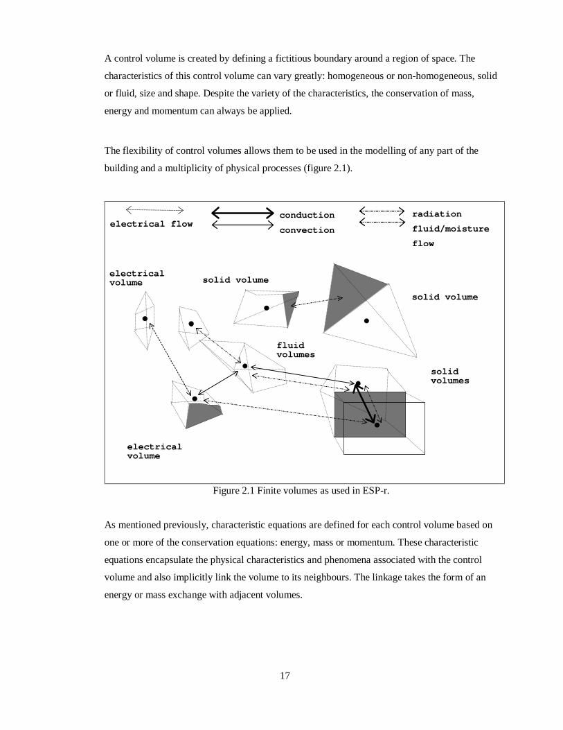
The flexibility of control volumes allows them to be used in the modelling of any part of the
building and a multiplicity of physical processes (figure 2.1).
Figure 2.1 Finite volumes as used in ESP-r.
As mentioned previously, characteristic equations are defined for each control volume based on
one or more of the conservation equations: energy, mass or momentum. These characteristic
equations encapsulate the physical characteristics and phenomena associated with the control
volume and also implicitly link the volume to its neighbours. The linkage takes the form of an
energy or mass exchange with adjacent volumes.
electricalvolume
solidvolumes
solid volume
solid volumeelectricalvolume
fluidvolumes
conduction
convection
radiation
fluid/moisture
flow
electrical flow

18
The following paragraphs demonstrate applications of the control volume principle in ESP-r.
Knowledge of the application of control volumes in a thermal context is crucial to the
understanding of their application in modelling the electrical energy subsystem. This also gives
an insight into how thermal and electrical systems can be modelled in a truly integrated fashion,
by using the same modelling technique for both.
Note that the derivations of the control volume characteristic equations that follow are only
intended to introduce the reader to this approach to modelling the building. A more complete and
rigorous treatment of the theory behind control volumes and ESP-r is given by Clarke [1].
2.2.1 The Control Volume Applied to a Zone
This section deals with the application of the control volumes to the most important element of a
building model: the enclosed air (fluid) volumes that constitute the thermal zones of the
building. They are also perhaps the most thermodynamically interesting areas of the building, as
the modeller can successively apply energy, mass and momentum balances to a volume of fluid,
depending on the rigour of analysis required. In addition, the zones of the building are subject to
many varied energy exchanges: heat and vapour gains from occupants, plant interaction, solar
energy transmitted through glazing, infiltration, air exchange with other spaces etc. Finally, and
as a link to chapter 3, a coupling between this control volume and the electrical ‘world’ is the
heat gain to the building interior from lights and other electrical appliances. Other
thermal/electrical couplings are explored later.
The flexibility of the control volumes in analysing physical problems at varying levels of
complexity will be shown in this section, as the control volume technique will be applied with
increasing rigour to the zone. Subsequent sections will demonstrate the application of the control
volume technique to the fluid volume’s bounding and peripheral elements: fabric and
conditioning plant.
At the most basic level of detail a single control volume, represented by a single node, can be
used to describe the volume of fluid that constitutes the zone. This volume is bounded by solid
constructions and is subject to heat transfer by convection, fluid exchange with its neighbouring

19
volumes, infiltration from the exterior, heat and vapour gains from occupants, plant interaction,
etc. The fundamental equation governing these exchanges is an energy balance of the form
∑=
=n
jij
iiii q
tcV
1∂∂θρ . (2.1)
Vi is the volume (m3) of the fluid volume i, ρi is its average density (kg/m3), ci is its average
specific heat (J/kgK) and θi is its average temperature (oC). The left-hand side of the equation
represents the thermal capacitance of the fluid volume, while the qijj
n
=∑
1
term is the sum of the
energy fluxes (W) that interact with the control volume. These are of three types: surface to fluid
heat transfer, fluid flow from other fluid volumes and sensible energy gains from sources inside
the zone.
The general form of the equation describing the convective heat transfer (W) between a surface s
and the fluid volume i is
)( issscis Ahq θθ −= . (2.2)
θs is the surface temperature, As is the contact area (m2) with the fluid volume and hcs is the heat
transfer coefficient (W/m2K). Note that in this equation, a linear convective heat transfer
coefficient is used to describe the non-linear process of convective heat transfer. This is done to
preserve the overall linearity of the equation, eventually enabling fast, efficient solution methods
to be applied in the solution of the equation sets that describe the zonal energy flows (this is
discussed in section 2.3.1). ESP-r’s treatment of non-linear processes using linear coefficients is
explained in section 2.3.3.
The from of the equation describing the energy exchange (W) due to fluid flow between two
fluid volumes i and k is
)( ijjijij cmq θθ −= & (2.3)

20
&mij is the pressure/temperature driven mass flow rate (kg/s) between the two volumes,
calculation of this value is dealt with in the next section. cj is the specific heat of the fluid
transferred from the neighbouring volume and θj is its temperature.
The gains from sources inside the zone (W) can be lumped together into a single term, qi, which
includes such phenomena as sensible heat gains from the lighting, small power loads and the
sensible heat gain from occupants.
The basic equations for the control volume energy balance can be applied to the fluid volume
shown in figure 2.2.
Figure 2.2 Energy exchanges associated with a zone fluid volume
The volume is bounded by nine different surfaces, each of which exchange energy by convection
with the air volume. There are also four fluid exchanges with surrounding fluid volumes (some
of which may be exchanges with the external environment). Applying the previously defined
equations to the fluid volume of figure 2.2 gives the following expression
∑∑==
+−+−=4
1
9
1
)()(k
iikkikijsj
jsijci
iii qcmAht
cV θθθθ∂
∂θρ & . (2.4)
fluid/fluidexchange
surface/fluidexchange

21
Applying a backward difference scheme to the partial derivative term, over some finite time
interval, ∆t (s), the following expression emerges.
( )∑∑
==
∆+
+−+−=∆
− 4
1
9
1
)()(k
ti
ti
tkk
tik
ti
tsj
jjsij
tc
ti
ttiiii qcmAht
cV θθθθθθρ& . (2.5)
Dividing by the volume Vi:
( )i
ti
i
k
ti
tkk
tik
i
ti
tsj
jjsij
tct
itt
iii
V
q
V
cm
V
Ah
t
c+
−+
−=
∆− ∑∑
==∆+
4
1
9
1)()( θθθθ
θθρ&
(2.6)
For reasons of numerical stability during the solution process, ESP-r uses a mixed
implicit/explicit form of the heat balance equation [3]. The implicit form is given by
( )
.
)()(4
1
9
1
i
tti
i
k
tti
ttkk
ttik
i
tti
ttsj
jjsij
ttct
itt
iii
V
q
V
cm
V
Ah
t
c
∆+
=
∆+∆+∆+∆+∆+
=
∆+∆+
+
−+
−=
∆− ∑∑ θθθθ
θθρ&
(2.7)
Adding equations 2.6 and 2.7 together, re-arranging and grouping the future time step terms on
the right hand side gives the mixed expression for the energy balance at fluid node i.

22
.2
2
4
1
9
1
4
1
9
1
4
1
9
1
4
1
9
1
i
ti
i
k
tkk
tik
i
j
tsjjsij
tc
ti
i
kk
tik
i
jjsij
tc
iii
i
tti
i
k
ttkk
ttik
i
j
ttsjjsij
ttc
tti
i
kk
ttik
i
jjsij
ttc
ii
V
q
V
cm
V
Ah
V
cm
V
Ah
t
cV
V
q
V
cm
V
Ah
V
cm
V
Ah
t
c
−−−
++∆
=
+++
++∆
∑∑∑∑
∑∑
∑∑
====
∆+=
∆+∆+
=
∆+∆+
∆+=
∆+
=
∆+
θθθρ
θθ
θρ
&&
&
&
(2.8)
This is the basic equation used by ESP-r in the calculation of a fluid volume’s temperature. The
bracketed term in front of the nodal temperature θit+∆t is known as the self-coupling coefficient.
The terms in front of the other future time step nodal temperatures are the cross coupling
coefficients. These provide the link to the other nodes which exchange energy with node i. The
right hand side of the equation can be regarded as a single coefficient comprising calculated
present time step terms and known boundary conditions.
The above equation describes the one-dimensional heat flow associated with the air volume.
ESP-r deals with three-dimensional heat flow in the air volume using integrated computational
fluid dynamics (CFD). This is discussed in the section 2.2.3. ESP-r can also deal with two and
three dimensional heat flow calculations in solid elements. The use of control volumes in
modelling the solid structure of the building is discussed later.
For the sake of clarity in the derived equations 2.1-8 the nodal thermophysical properties ρ, k
and c, are shown as time-invariant. However, these properties can vary with temperature and
hence become functions of the, as yet unknown, future time step temperature θit+∆t. ESP-r can
deal with these time-varying thermophysical properties using the techniques outlined in section
2.3.3.

23
Note that the derived balance equations contains terms relating to bulk air (fluid) flow ( &m ); the
principles of the control volume can be extended to model this phenomena as well.
Also note that the derived characteristic equation gives equal weighting to the implicit and
explicit terms, the so-called Crank-Nicholson formulation of the equation. It should be kept in
mind when reading the derivations that follow, that ESP-r allows the user to change the
weighting between the implicit and explicit components of the characteristic equations.
2.2.2 Application of a Mass Balance to the Fluid Volume
As with the plant and zonal energy equations, the fluid flow equations for a control volume are
derived from a basic balance equation; this assumes that the sum of the connected mass flow
rates is zero and that no mass is stored:
01
=∑=
n
jijm& . (2.9)
&mij is the mass flow rate between nodes i and j (kg/s) and n is the number of connected fluid
volumes that exchange mass with node i. Consider the following room, described in the previous
section, connected to four other volumes i+1….i+4 by various openings.

24
Figure 2.3 The control volume representation of a fluid volume.
Flow between volumes is generally governed by a non-linear function of the pressure difference
across the opening separating them:
)(),( ,, yxyxyx pfppfm ∆==& . (2.10)
Here pn is the pressure of the node (Pa). The total pressure difference across an opening is a
combination of static pressure difference and pressure differences caused by height and density
variations between the two connected fluid volumes (i.e. buoyancy effects).
The general form of the balance equation for the node i is
0)()()()( 4,3,2,1, =∆+∆+∆+∆ ++++ iiiiiiii pfpfpfpf . (2.11)
If all the openings into the zone are small cracks (i.e. through small window openings and under
doors) then the non-linear equations governing the flow are of the general form
nyxyxx pm )( ,, ∆= κρ& , (2.12)
i
i+1
i+2
i+4
i+3
a fluid flow path
opening

25
where n and κ are empirically derived values dependant upon the opening characteristics (area,
hydraulic perimeter, length, etc.). The balance equation is therefore
.0)(
)()()(
4,4,4
3,3,32,221,1,1
=∆+
∆+∆+∆
+++
+++++++++
diiiii
ciiiii
biiii
aiiiii
p
ppp
κρ
κρκρκρ(2.13)
Equation 2.13 is a non-linear function of the inter-nodal pressure differences, which describes
the flow balance at node i. Note that the governing equations of mass flow through an opening
need not be the same as equation 2.13, but can be any function of the pressure difference across
it.
Many researchers (e.g. Cockroft [4]) have developed expressions of the form of equation 2.10
that describe the flow of fluids across building components (doors, cracks, ducts piping, etc.)
2.2.3 Application of Energy Mass and Momentum Balances (CFD)
The representation of a zone using a single control volume as described previously is easy for
the modeller to conceptualise, computationally efficient and simple to implement in simulation
tools. This single control volume model of the zone provides the modeller with information
regarding the bulk temperature and air flows within the room. However, the implicit assumption
behind the use of the single air volume is that the air is well mixed; this is sometimes not the
case as temperature stratification, stagnant areas, thermal plumes and cold down draughts
usually exist in heated rooms. If these phenomena are to be modelled, and more detailed design
information is required, such as room air velocities or room temperature distribution, then a
more detailed approach to modelling the zone air volume must be taken.

26
Figure 2.4 The zone subdivided into smaller control volumes.
Subdivision of the zone into many smaller control volumes and the addition of a momentum
balance and perhaps a concentration balance (e.g. the quantity of water or contaminant in each
volume) to each, introduces the prospect of integration of computational fluid dynamics (CFD)
into the building simulation. The use of CFD to model the zone allows not only the
determination of bulk fluid energy flows, but also the airflow patterns and temperature
distribution as well. However, it should be noted that increasing detail is achieved at the expense
of increasing computational and data input overhead. The advantages, disadvantages and
applicability of integrating CFD into a simulation must be carefully considered by the modeller.
The equations for each CFD control volume (or cell) involve the conservation of mass
momentum, energy and concentration. These equations have the following general form:
φφ ∂∂φ
∂∂ρφ
∂∂
Sxxt i
ii
+Γ= )( . (2.14)
Here φ is a transport variable, Γφ is a diffusion coefficient and Sφ is a source term.
Indoor air flows are complex, chaotic phenomena that can be simulated using turbulent transport
models. In these models the fundamental equations are time-averaged and are augmented by a
CFD controlvolumes

27
further two equations representing local turbulent energy, k (J), and its dissipation, ε (J/s); these
equations form the k-ε turbulence model.
Substituting the terms shown in the table below into equation 2.14 gives the time-averaged
conservation equations for mass, energy, momentum and concentration, plus the equations for
turbulent energy and its dissipation rate.
Equation type φ Γφ Sφ
Continuity (mass) 1 - -Momentum Vi µef
ij
i
i
jef
ii
gx
V
x
V
xx
P ρµ −
∂∂
+
∂∂
∂∂+
∂∂−
Energy T ΓT
pc
q ′′′
Concentration C ΓC m ′′′&
Turbulent energy k
k
ef
σµ bD GCG −− ρε
Energy dissipation ε
εσµef
bGk
Ck
CGk
Cεερε
3
2
21 −−
;Pr T
tT σ
µµ +=Γ ;C
t
CC
S σµµ +=Γ µµµ += tef ; ),( CTρρ =
∂∂+
∂∂=
iC
tC
iT
TTb x
C
x
TgG
σµβ
σµβ ;
j
i
i
j
j
it x
V
x
V
x
VG
∂∂
∂∂
+∂∂
= µ
CD=1.0; CD=1.44; C2=1.92; 0.1=kσ ; 3.1=εσ ; 9.0=Tσ ; 9.0=Cσ
Table 2.1 Diffusion coefficients and source terms for the k-ε model.
The V terms in the equations represents time-averaged velocity components (m/s), while T and P
represent time-averaged temperature (K) and pressure (Pa) respectively; µt is the eddy-viscosity
(kg/ms) of the flow, while q ′′′ and m ′′′ are the per-unit volume rates of heat (W/m3) and mass
generation (kg/m3); Pr is the Prandtl number. The other symbols used in the equations represent
their usual thermophysical properties.
The equations of the k-ε model are solved iteratively to yield the temperature and velocity
distributions within the space described by the CFD control volumes. However, the k-ε
turbulence model is valid only for high Reynolds Numbers. At low Reynolds Numbers, typically

28
encountered at wall surfaces due to viscous effects, log-law wall functions are required to
describe the velocity and temperature distributions.
Negrao [5] describes the basic theory behind CFD modelling and how it is applied within the
context of a building simulation. Clarke and Beausoleil-Morrison [6] describe how CFD has
been fully integrated into the ESP-r system: a graded approach is taken, in which the CFD and
building model can interact at varying levels of complexity. At the simplest level of integration
the CFD model is run to provide the surface convective heat transfer coefficients (the hc term of
equation 2.2) for the thermal model. At the most complex level of integration, the CFD model is
fully coupled with both the thermal zones and the fluid flow network (which provides mass flow
and velocity boundary conditions). The CFD solution then provides air temperature and velocity
distributions within the zone, as well as air flow information to the fluid flow network.
The surface convective heat transfer coefficients calculated using the CFD model can be used
directly with the group of control volumes described in the next section: those which describe
the bounding multi-layered construction of the zone fluid volumes.
The integration of CFD into ESP-r illustrates the trend towards increased rigour and complexity
in building energy modelling. This trend is driven by the desire to model the physical processes
occurring within the building in a more realistic fashion. A result of this move towards
integration is that once separate modelling tasks such as CFD, lighting analysis and building
thermal simulation are now performed simultaneously within an integrated model. The addition
of electrical power flow modelling to building simulation is another step in this direction.
2.2.4 The Control Volume Applied to the Building Fabric
In ESP-r multi-layered constructions are used to represent the solid elements which make up the
building fabric and provide the physical boundaries to the zones. Consider now the application
of the control volume principle to the fundamental heat transfer process occurring in these solid
elements: conduction, convection and radiation.

29
Figure 2.5 Heat transfer in a multi-layered construction.
It is possible to represent the surface layer of the construction shown in figure 2.5 using three
control volumes: a homogeneous material volume, a surface volume and a mixed property
volume located at the boundary with the next layer of material. Each is of dimensions ∆xn, ∆yn,
∆zn, (m), where ∆xn is the thickness, ∆yn the breadth and ∆zn the height of element n. Consider
firstly the application to the homogeneous volume, represented by node i:
Figure 2.6 A control volume representation of a layer of homogeneous material.
convection
homogeneous layer
∆xi
mixed layer surface layer
i
conduction
i+1
radiation
i-1
∆zi
∆yi
i+1i-1 i

30
The following is the basic heat balance equation for one dimensional heat flow along the x-axis
in this element.
∑=
=n
jij
iiii q
tVc
1∂∂θρ (2.15)
Note that the basic equation for the solid control volumes is identical to that applied to the fluid
volume (equation 2.1).
Again, applying a backwards difference scheme to the partial derivative term over some finite
time interval ∆t (s), and considering the heat fluxes shown in figure 2.5 the following expression
emerges.
eti
tii
tii
ti
ttiiii qqq
t
Vc++=
∆−
−+
∆+
1,1,
)( θθρ. (2.16)
θ t represents the temperature at the current time t and θ t+∆t the temperature at some future time
t+∆t. The qit
e (W) term included in the equation is a general heat generation term that can be
adapted to suit various temperature independent phenomena, e.g. plant heat input or solar
absorption. The conductive heat transfers with adjacent nodes (W), qi,i+1, and qi,i-1, can also be
expressed in discrete form:
i
ti
tiiiii
iit
x
yzkq
∆−∆∆
= +++
)( 11,1,
θθ, (2.17)
similarly,
i
ti
tiiiiit
ii x
yzkq
∆−∆∆
= −−−
)( 11,1,
θθ. (2.18)
Where km,n represents the conductivity (W/mK) of the material between the two nodes m and n.
Substituting equations 2.17 and 2.18 back into equation 2.16 gives

31
eti
i
ti
tiiiii
i
ti
tiiiii
ti
ttiiii q
x
yzk
x
yzk
t
Vc+
∆−∆∆
+∆
−∆∆=
∆− −−++
∆+ )()()( 11,11, θθθθθθρ. (2.19)
This is the explicit form of the heat balance equation for the control volume represented by node
i. The implicit form of the equation is given by
tt
ei
i
tti
ttiiiii
i
tti
ttiiiii
ti
ttiiii
q
x
yzk
x
yzk
t
Vc
∆+
∆+∆+−−
∆+∆+++
∆+
+
∆−∆∆
+∆
−∆∆=
∆− )()()( 11,11, θθθθθθρ
(2.20)
Adding 2.19 and 2.20 together gives the following mixed expression.
.)()(
)()()(2
11,11,
11,11,
tteie
ti
i
tti
ttiiiii
i
tti
ttiiiii
i
tti
ttiiiii
i
tti
ttiiiii
ti
ttiiii
qqx
yzk
x
yzk
x
yzk
x
yzk
t
Vc
∆+∆+∆+
−−∆+∆+
++
∆+∆+−−
∆+∆+++
∆+
++∆
−∆∆+
∆−∆∆
+∆
−∆∆+
∆−∆∆
=∆
−
θθθθ
θθθθθθρ
(2.21)
Dividing by the volume Vi = (∆x∆y∆z)i and grouping the future time row terms (t+∆t) on the left
hand side of the equation gives
( )
( ) .2
2
12
1,12
1,
2
1,1,
12
1,12
1,
2
1,1,
i
teit
i
i
iiti
i
iiti
i
iiiiii
i
tteitt
i
i
iitti
i
iitti
i
iiiiii
zyx
q
x
k
x
k
x
kk
t
c
zyx
q
x
k
x
k
x
kk
t
c
∆∆∆+
∆+
∆+
∆
++
∆=
∆∆∆−
∆−
∆−
∆
++
∆
−−
++−+
∆+∆+
−−∆+
++∆+−+
θθθρ
θθθρ
(2.22)
This is the basic energy balance equation used by ESP-r in the calculation of nodal temperatures
in a homogeneous layer of material. Note the similarity between this equation and the energy
balance derived for the fluid volume (equation 2.8).

32
Similar equations can be constructed for the control volume at the surface layer of a material,
represented by node i+1, and the mixed property element, node i-1, located at the boundary with
another layer.
A control volume as shown in figure 2.7 represents the surface layer of the construction, shown
in figure 2.5
Figure 2.7 A control volume representation of the surface layer of a material.
Considering only one-dimensional conduction and applying the same procedures as were used
with the homogeneous element, the following equation for the energy balance in the control
volume emerges.
∆xi+1
∆zi+1
∆yi+1
i+1i

33
( )
( ) .
2
2
1
1
1
1
1
1,
21
1,1
1
1
1 1
1,
21
1,11
1
1
1
1
1
1,
21
1,1
1
1
1 1
1,
21
1,11
+
+
+
+
=
+
+
++
+
+
= +
+
+
+++
+
∆++∆+
+
+
=
∆++∆+
+
+∆++
+
+
= +
+
+
+++
∆∆∆+
∆+
∆+
∆+
∆
+∆
+∆
+∆
=
∆∆∆−
∆−
∆−
∆−
∆+
∆+
∆+
∆
∑∑
∑∑
i
tirt
ai
ic
n
s
tsisrt
i
i
iiti
i
icn
s i
isr
i
iiii
i
ttirtt
ai
ic
n
s
ttsisrtt
i
i
iitti
i
icn
s i
isr
i
iiii
zyx
q
x
h
t
h
x
k
x
h
x
h
x
k
t
c
zyx
q
x
h
t
h
x
k
x
h
x
h
x
k
t
c
θ
θθθρ
θ
θθθρ
(2.23)
Again, the self-coupling coefficient, cross coupling coefficients and right hand side coefficient
are evident in the equation structure. However additional terms are included to account for
physical phenomena occurring at the surface of a material. hc is the convective heat transfer
coefficient, described in section 2.2.1. θa is the temperature of the adjacent air volume.
hr s is
n
, +=
∑ 11
are the radiative heat transfer coefficients (W) that characterise the long wave radiant
heat transfer between this and the n other surfaces in the zone. The term qr represents solar and
other radiant gains (W) to the surface (e.g. from plant and occupants).
The final type of element shown in figure 2.5 is the mixed property control volume, represented
by node i-1, this is shown in more detail in figure 2.8.

34
Figure 2.8 The control volume representation of a mixed property region.
In a similar fashion to the homogeneous and surface regions, the following equation describing
the energy balance in the finite volume can be derived.
( )
( ) 1
1
21,21,1
11,2
1,21,1
11,
11,21,1
11,2
1,21,1
11,11
1
1
21,21,1
11,2
1,21,1
11,
11,21,1
11,2
1,21,1
11,11
)(
2
)(
2
)(
2
)(
22
)(
2
)(
2
)(
2
)(
22
−
−
−−−−−
−−−
−−−−
−−
−−−−−
−−−
−−−−
−−−−
−
∆+−
∆+−
−−−−
−−−∆+
−−−−
−−
∆+−
−−−−
−−−
−−−−
−−−−
∆∆∆+
∆+∆∆
∆++
∆+∆∆∆+
+
∆+∆∆
∆++
∆+∆∆∆+
+∆
=
∆∆∆−
∆+∆∆
∆+−
∆+∆∆∆+
−
∆+∆∆
∆++
∆+∆∆∆+
+∆
i
eti
ti
iiiii
iiiti
iiiii
iii
ti
iiiii
iii
iiiii
iiiii
i
tt
ei
tti
iiiii
iiitti
iiiii
iii
tti
iiiii
iii
iiiii
iiiii
zyx
q
Rxxx
xRk
Rxxx
xRk
Rxxx
xRk
Rxxx
xRk
t
c
zyx
q
Rxxx
xRk
Rxxx
xRk
Rxxx
xRk
Rxxx
xRk
t
c
θθ
θρ
θθ
θρ
(2.24)
material interface
i-1i-2
∆xi-1
i
∆zi-1
∆yi-1
∆xi,i-1
etc.

35
Note that the density ρi-1 and the specific heat cp i-1of this control volume are a volume weighted
average of its two constituent materials. R represents an added resistance (m2K/W) at the
material interface.
Also note that the equations shown here deal only with one-dimensional heat conduction. As
was noted earlier, ESP-r can also model two or three-dimensional heat flow in elements of the
building structure. Clarke [2] outlines how the control volume method is extended to deal with
this.
The previous sections illustrated the control volume technique applied to the characteristic
elements of the zone: the fluid volume and its bounding constructions. Equations describing the
energy flow in those elements were derived. Clarke [2] uses the same methods to develop
equations for other constituents of a thermal zone: transparent constructions, air gaps etc.
2.2.5 The Control Volume Applied to Plant Components
As with the zones that make up the building model, the control volume technique can also be
used to derive the equation sets describing a building’s plant network. In ESP-r the plant
network consists of a coupled group of plant component models, each of these models being
described by one or more control volumes. Consider the application of the technique to a typical
plant component; an air/water heat exchanger. The component can be described using three
control volumes: one for the fluid, one for the air and one for the solid elements of the
component. More or less control volumes can be used, depending on the level of detail required
by the modeller. This representation of the plant component is shown in figure 2.9.

36
Figure 2.9 The control volume representation of a air/water heat exchanger.
The energy balance equation 2.1 can also be applied to the control volumes of the plant
component. Discretising this equation for the solid node, i, of the plant component gives
( )∞−+
∆+
++=∆
−,1,1, iiiii
ti
tti
iii qqqt
Vcθθρ . (2.25)
Where qi,i+1, qi,i-1 are the heat exchanges (W) with the neighbouring fluid and air volumes of the
heat exchanger, qi,∞ is the heat exchange (W) with the environment surrounding the plant
component. qi,i+1, and qi,i-1 can be expressed as a function of temperature:
)( 11,1,1, iiiiiiii Ahq θθ −= ++++ ; (2.26)
similarly,
).( 11,1,1, iiiiiiii Ahq θθ −= −−−− (2.27)
Ai,n are the contact areas (m2) between the volume represented by node i and connected volumes:
in this case the contact area of the neighbouring air and fluid streams with the solid casing. hi,n
are the heat transfer coefficients between the fluid streams and the casing (W/m2K). As with the
i+2
i-1i+1
i
fluidnode
solid node
air node
heat exchange i-2fluid flow

37
building equations, linear coefficients are used in the representation of non-linear heat transfer
exchanges between the fluids and the casing. Again, refer to section 2.3.3 for an explanation of
how ESP-r deals with these non-linear processes.
The exchange between the plant component and the environment can be expressed in a similar
form to equations 2.26 and 2.27
).(,, iii hq θθ −= ∞∞∞ (2.28)
Where hi,∞ is the heat transfer coefficient between the control volume and the environment at a
temperature θ∞.
Substituting 2.26-8 into equation 2.25 at some time t, gives the implicit form of the control
volume energy balance equation for node i.
( )).()()( ,,11,1,11,1,
ti
tii
ti
tiiiii
ti
tiiiii
ti
tti
iii AhAhAht
Vc θθθθθθθθρ −+−+−=∆
−∞∞∞−−−+++
∆+
(2.29)
As with the building equation sets, ESP-r uses a mixed implicit/explicit expression as the
characteristic equation. The implicit form of equation 2.29 is
( )
).(
)()(
,,
11,1,11,1,
tti
ttii
tti
ttiiiii
tti
ttiiiii
ti
tti
iii
Ah
AhAht
Vc
∆+∆+∞∞∞
∆+∆+−−−
∆+∆++++
∆+
−+
−+−=∆
−
θθ
θθθθθθρ
(2.30)
Adding the implicit and explicit expressions and grouping future time step terms on the left-hand
side of the equation gives

38
.
2
2
,,
11,1,11,1,,,1,1,1,1,
,,
11,1,11,1,,,1,1,1,1,
tii
tiiiii
tiiiii
ti
iiiiiiiiiiiii
ttii
ttiiiii
ttiiiii
tti
iiiiiiiiiiiii
Ah
AhAht
AhAhAhVc
Ah
AhAht
AhAhAhVc
∞∞∞
−−−+++∞∞−−++
∆+∞∞∞
∆+−−−
∆++++
∆+∞∞−−++
+
++
∆
+++=
−
−−
∆
+++
θ
θθθρ
θ
θθθρ
(2.31)
The plant control volume characteristic equation has an identical structure to those derived for
the multi-layered construction, with a self-coupling coefficient, cross coupling coefficients
linking adjacent control volumes and a right hand side containing previously calculated and
known values.
Turning to the other two control volumes in the heat exchanger and applying the same basic
energy balance as was as used with node i, two characteristic equations can be derived. Note,
that in these two cases energy is exchanged by fluid transfers with adjacent volumes where the
heat exchange (W) between two nodes x and y, coupled by fluid flow is given by
)(,, yxyyxyx cmq θθ −= & . (2.32)
The air in the heat exchanger is a binary mixture, consisting of both dry air and water vapour,
hence in equation 2.33 subscript v refers to vapour properties and a refers to dry air properties,
&m refers to a mass flow rate of air or vapour (kg/s). The heat exchange with nodes coupled by
fluid flow is given by
)()( ,,, yxypayaxyxyvyxvyx cmcmq θθθθ −+−= && . (2.33)
The air and vapour are assumed to be at the same temperature.

39
For the air volume node i-1, the energy balance equation is therefore
[ ]
[ ]
.
2
2
1,1,22
11,1,
1,1,22
11,1,
22,122,1
22,122,1
111111
22,122,1
22,122,1
111111
tiiiii
tia
ta
tiv
tv
tiiiiia
tav
tv
aaavvv
ttiiiii
ttia
tta
ttiv
ttv
ttiiiiia
ttav
ttv
aaavvv
Ahcmcm
Ahcmcmt
VcVc
Ahcmcm
Ahcmcmt
VcVc
iiiiii
iiiiii
iiiiii
iiiiii
iiiiii
iiiiii
θθθ
θρρ
θθθ
θρρ
−−−−
−−−
∆+−−
∆+−
∆+∆+−
∆+
∆+−−−
∆+∆+
+++
+++
∆
+=
−−−
+++
∆
+
−−−−−−
−−−−−−
−−−−−−
−−−−−−
−−−−−−
−−−−−−
&&
&&
&&
&&
(2.34)
For the fluid volume represented by node i+1, the energy balance equation is
[ ]
[ ]
.
2
2
1,1,22
11,1,22,1111
1,1,222,1
11,1,2111
2,1
2,1
tiiiii
tii
tv
tiiiiii
tii
iii
ttiiiii
ttii
ttii
ttiiiiiiv
ttv
iii
Ahcm
Ahcmt
Vc
Ahcm
Ahcmt
Vc
ii
ii
θθ
θρ
θθ
θρ
++++
−−−+++−−−
∆+++
∆+++
∆+++
∆++++−
∆++++
++
++
∆=
−−
++
∆
++
++
&
&
&
&
(2.35)
Note that, as with the equations for the zonal fluid volume, the energy equations contain terms
relating to fluid flow. Again these would be evaluated using a mass balance technique applied to
a fluid control volume.
Clarke [2], Tang [7], Aasem [8] and Hensen [9] apply the control volume modelling technique to
a variety of plant components, while Mclean [10] applies it to solar energy systems. The
resulting library of developed component models allows the simulation of air conditioning
systems, hot water heating systems and mixed air/hot water systems as a plant network in ESP-r.
Chow [11] has extended the principle of the control volumes in plant modelling by identifying

40
27 fundamental ‘primitive parts’, which are essentially characteristic control volumes describing
the basic thermodynamic processes occurring in air conditioning systems. The aim of this work
is that any plant component can be described and modelled from coupled groups of these
primitive parts.
2.3 Treatment and Solution of the Finite Volume Equation Sets
The previous sections demonstrate the applicability of the control volume to different aspects of
the building and how for each, a characteristic equation can be extracted. Having derived these
equations, it is necessary to arrange them in a form suitable for solution within the context of a
transient energy simulation.
Two different types of equation were derived in sections 2.2.1-2.2.5: the linearised zonal and
plant equations and the non-linear, fluid flow equations. Grouping each set of equations
according to subsystem and type allows them to be processed in the most appropriate manner:
direct methods for the linearised plant and building equations and iterative techniques for the
non-linear fluid flow equations. Note that the processing method is determined by the linearity
or non-linearity of the system’s characteristic equations, rather than the linearity or non-linearity
of the system itself (i.e. air flow is a linear system modelled using non-linear equations, the
reverse is true for the building and plant energy flows).
All of the derived equations contain terms relating to other coupled volumes, so a simultaneous
solution is required. The following sections describe the methods of solution for the building,
plant and fluid flow equation sets. Section 2.4 shows how they are solved simultaneously by a
process of iterative handshaking.
2.3.1 Zonal Energy Equations
The equations which describe the energy flows in the thermal zones of the model have the
general form

41
.11
11
11111
11111
n
n
j
tnn
tjnj
tnn
n
j
ttnn
ttjnj
ttnn
n
j
tn
tjj
tn
j
ttttjj
tt
dqcbaqcba
dqcbaqcba
+++=++
+++=++
∑∑
∑∑
==
∆+∆+∆+
==
∆+∆+∆+
θθθθ
θθθθ
M (2.36)
For any node i,θi is a nodal temperature, ai the self-coupling coefficient, bijj
n
=∑
1
are the cross
coupling coefficients to connected nodes, ci is the coefficient for the heat generation term, qi and
di are any ‘known’ boundary condition (e.g. climate parameters). The terms on the right-hand-
side represent the unknown future time step of the simulation, t t+ ∆ , while the left-hand-side
terms contains the present time step and known boundary terms.
In matrix form, the set of zonal equations can be written as
ZCBxAx =+=∆+ )( ttt . (2.37)
Where A is the matrix of future time step nodal self and cross-coupling coefficients, B is the
matrix of present time step coefficients and C is the matrix of known terms and boundary
conditions. Z is the combined matrix of solved present time step and known terms, x t t+∆ and
x t are column matrices of nodal temperatures and heat injections at the present and future time
steps respectively.
Solution of equation 2.37 can be achieved by multiplication of both sides by the inverse of A, to
give the unknown temperatures and heat injections. Unfortunately, the A matrix is characterised
by its size and sparsity (in the typical building model the A matrix will contain thousands of
entries, most of them zero). Inversion of this type of matrix at each time step in a simulation is
both a computationally expensive and time-consuming process. This solution method is
therefore unacceptable for use in a simulation tool. ESP-r uses a more efficient, customised
solution process. Instead of forming one large matrix equation for the whole building, smaller
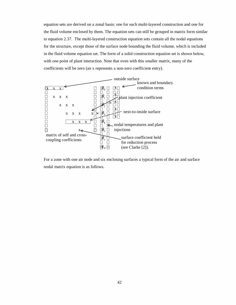
42
equation sets are derived on a zonal basis: one for each multi-layered construction and one for
the fluid volume enclosed by them. The equation sets can still be grouped in matrix form similar
to equation 2.37. The multi-layered construction equation sets contain all the nodal equations
for the structure, except those of the surface node bounding the fluid volume, which is included
in the fluid volume equation set. The form of a solid construction equation set is shown below,
with one point of plant interaction. Note that even with this smaller matrix, many of the
coefficients will be zero (an x represents a non-zero coefficient entry).
For a zone with one air node and six enclosing surfaces a typical form of the air and surface
nodal matrix equation is as follows.
x x x
x x x
x x x
x x x x
x x x
x
x
x
x
x
x
×
=
θ
θ
θ
θ
θ
θ
θ
0
1
2
3
4
5
s
pq
outside surface
surface coefficient heldfor reduction process(see Clarke [2]).
next-to-inside surface
plant injection coefficient
matrix of self and cross-coupling coefficients
known and boundarycondition terms
nodal temperatures and plantinjections

43
Subscript sn refers to a surface node, sn-1 refers to the next-to-inside surface node and θa is the
temperature of the zone air node. The aim of the solution method is to process the zonal equation
sets, taking into account the interaction of other factors, such as plant input and control
objectives, on the eventual solution. The control objectives are central to the processing of the
equation sets and require some explanation.
The basis of control in ESP-r is the control loop, through which a property of a node is sensed
and an appropriate action taken at an actuation point, which may be the same or another node in
the model. The aim of the actuation is to bring the sensed nodal variable to a desired value. As
an example: it is possible to change the temperature of air delivered to a room by altering the
flow of hot water to a heating coil located in an air handling unit in another part of the building.
The operation of control in ESP-r is discussed at length by Clarke [2].
Returning to the solution process, this proceeds using a forward reduction technique, in which
the equation set of each multi-layered construction is processed so that one characteristic
equation is derived:
x x x x x x x x
x x x x x x x x
x x x x x x x x
x x x x x x x x
x x x x x x x x
x x x x x x x
x x x x x
x x
×
−
−
−
θθθθ
θθθ
s
s
s
s
s
s
a
1 1
1
2 1
2
6 1
6
M
M
M
M
M
M
=
x
x
x
x
x
x
x
x
inside surface coefficient
air
volume
coefficients
s
next-to-inside surfacecoefficients
surface, next-to-insidesurface and airtemperatures
known andboundary conditionterms

44
Where a … j are the modified coefficients emerging from the reduction process. The
characteristic equation contains the essential properties of its associated equation set. Note that if
one of the nodes in a particular construction is a sensed node then an extra characteristic
equation is derived from the construction’s equation set. This extra equation incorporates the
temperature of the sensed node θc, as shown above, where the sensed node is 3. This control
temperature will be used in the final solution of the zonal energy equation.
The extracted equations are added, arithmetically, to the air volume equation set, which is in turn
forward reduced to a final characteristic equation for the entire zone:
a b cq di n c pi
nθ θ+ + =
=∑
1. (2.38)
Again, b, c and d are the modified nodal coefficients emerging from the final reduction process,
while aii
n
=∑
1
are the modified coefficients relating to the bounding temperatures of the zone,θ i ,
e.g. the temperatures of other connected zones or an external temperature. qp represents the
energy input from plant, while θc is the temperature of the sensed node in the zone. If previous
x x x
x x x
x x x
x x x x
x x x
x
x
x
x
x
x
(extra cha
reduces to
×
=
→ + + + =
+ + + =
θ
θ
θ
θ
θ
θ
θ
θ θ θ
θ θ θ
0
1
2
3
4
5
0 5
0 5 3
s
p
s p
p
q
a b c dq e
f g h iq j
racteristic equation
extracted for the control point)plant injectioncoefficient
control point
plant injection term
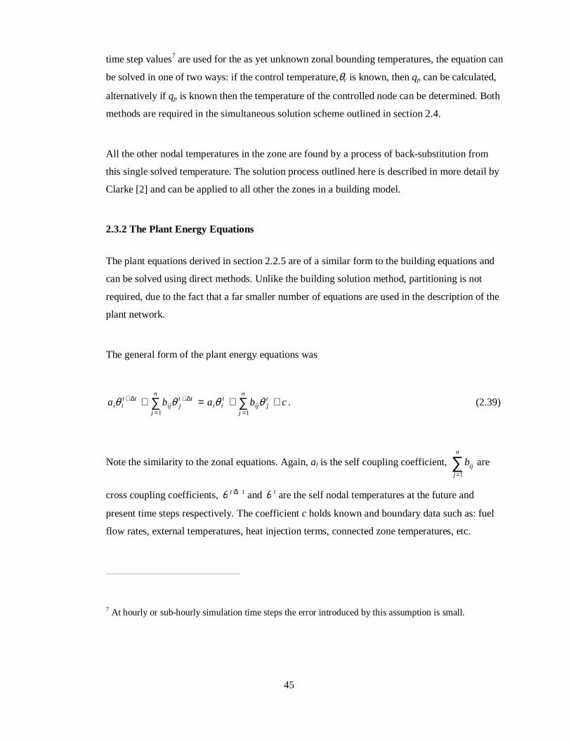
45
time step values7 are used for the as yet unknown zonal bounding temperatures, the equation can
be solved in one of two ways: if the control temperature,θc is known, then qp can be calculated,
alternatively if qp is known then the temperature of the controlled node can be determined. Both
methods are required in the simultaneous solution scheme outlined in section 2.4.
All the other nodal temperatures in the zone are found by a process of back-substitution from
this single solved temperature. The solution process outlined here is described in more detail by
Clarke [2] and can be applied to all other the zones in a building model.
2.3.2 The Plant Energy Equations
The plant equations derived in section 2.2.5 are of a similar form to the building equations and
can be solved using direct methods. Unlike the building solution method, partitioning is not
required, due to the fact that a far smaller number of equations are used in the description of the
plant network.
The general form of the plant energy equations was
cbaban
j
tjij
tii
n
j
ttjij
ttii ++=+ ∑∑
==
∆+∆+
11
θθθθ . (2.39)
Note the similarity to the zonal equations. Again, ai is the self coupling coefficient, bijj
n
=∑
1
are
cross coupling coefficients, θ t t+ ∆ and θ t are the self nodal temperatures at the future and
present time steps respectively. The coefficient c holds known and boundary data such as: fuel
flow rates, external temperatures, heat injection terms, connected zone temperatures, etc.
7 At hourly or sub-hourly simulation time steps the error introduced by this assumption is small.

46
As with the building equations, the set of plant equations can be written in matrix form:
A B Cθ θt t t+ = +∆ . (2.40)
Where the symbols have the same meaning as in equation 2.37. Solution for the future time step
nodal temperatures can be achieved by a direct method such as Gaussian elimination.
As with the building, the solution of the plant matrix is dictated by control interaction, where the
state of the system components is adjusted to bring about a desired control objective. The sensed
node for the plant control may be another plant component or another node in the building
model, e.g. the flow rate of cold water into a chiller coil may be controlled based on the relative
humidity in a thermal zone. Control is calculated for the plant network prior to solution of the
plant equations, hence the solution incorporates the effects of control action. The control action
is calculated based in the previous time step calculated values, i.e. one time step in arrears.
2.3.3 Treatment of Time-Varying and Non-Linear Processes
The equations derived for both building and plant are in linear-algebraic form, which allows
their solution using the efficient, direct methods outlined in sections 2.3.1 and 2.3.2. This
solution technique can be easily adapted to cope with the time-dependency of thermophysical
properties and/or non-linear heat transfer processes.
All the equations derived for the zones and plant contain terms relating to thermophysical
properties such as: density, specific heat capacity, conductivity etc. If these are considered time-
variant, e.g. as a function of temperature, then the value of the coefficients on the left-hand-side
(future time step) of the control volume energy equations cannot be determined, as the future
time step temperature is unknown. ESP-r’s solution to this problem is to calculate the material
properties based on the previously calculated time step temperatures. This has the advantage of
maintaining the linear form of the zonal and plant energy equations. If a great degree of accuracy
is required, or where certain processes or material properties are highly non-linear, then an
iterative solution mechanism can be employed, whereby the equation sets are solved assuming
the previous time step temperatures and processed to give the future time step solution. If the

47
difference between the assumed and calculated temperatures is too great then the solution is
repeated for that time step until convergence is obtained.
The same solution can be applied where non-linear heat transfer processes occur, e.g. long wave
radiant or convective heat transfer. In the zonal and plant equation sets these phenomena are
represented by linear coefficients8, whose values are calculated based on previous time step
temperature. Again, if a great degree of accuracy is required then the iterative mechanism can be
employed. In practice though, the assumption of previous time step temperatures proves
acceptable in hourly or sub-hourly building simulations.
2.3.4 The Fluid Flow Equations
The equations which govern the fluid flows (air and water) associated with the building are non-
linear. Hence, to achieve a solution of the fluid network equation set, an iterative solution
technique must be employed. Recall that the basic mass balance equation for each node in the
network was
01
.
=∑=
n
jijm .
Each flow associated with node i can be expressed as a function of pressure difference:
)(),(.
ijjiij pfppfm ∆== .
8 Note that the calculation leading to the determination of the heat transfer coefficient may be a
complicated process e.g. where coefficient can be calculated from a highly non-linear equation. This is
particularly true in the case of explicitly calculated radiative heat transfer coefficients for zones (see
Clarke[2]).

48
The sum of mass flows at a node i can therefore be expressed as a function of all the pressure
differences between it and all connected nodes:
0)(),,,,( ,1,2,1,1
.
=∆=∆∆∆∆= −=
∑ pininiii
n
j
fppppfm K . (2.41)
Expansion of the function about some known set of nodal pressures differences ∆pk by Taylor’s
series gives the following expression for an unknown set of nodal pressures ∆pk+1.
KK
K
+∆∆∆
∆++∆∆
∆
∆+∆∆
∆
∆
+∆∆∆
∆++∆∆
∆∆
+∆∆∆∆
+∆=∆ +
2,2
,
22
2,22,
22
1,21,
2
,,
2,2,
1,1,
1
))(()(
))(()(
))(()(
)()(
)()(
)()(
)()(
nini
ki
ii
ki
ii
ki
nini
ki
ii
ki
ii
kik
ik
i
pp
fp
p
fp
p
f
pp
fp
p
fp
p
fff
∂∂
∂∂
∂∂
∂∂
∂∂
∂∂
ppp
ppppp
(2.42)
Truncating terms above first order and rearranging gives
∆∆
∆∆
++∆∆∆
∆+∆∆
∆∆
=∆−∆ + )()(
)()(
)()(
)()( ,,
2,2,
1,1,
1ni
ni
ki
ii
ki
ii
kik
ik
i pp
fp
p
fp
p
fff
∂∂
∂∂
∂∂ ppp
pp K .
(2.43)
Applying this equation to all n nodes, and noting that at each node fi(∆pk) should be equal to zero
and jiji ppp ∆−∆=∆∆ )( , , the following matrix equation emerges.

49
∆∆
∆∆
×
∆∆
∆∆
−∆
∆−
∆∆
−
∆∆−
∆∆
∆∆−
∆∆−
∆∆
−∆
∆−
∆∆−
∆∆−
∆∆−
∆∆−
∆∆
−=
∆∆
∆∆
−
=−
−
−
= −−
−
−
−
−
−
−=
−=
−
∑
∑
∑
∑
n
n
m
j nn
k
nn
kn
n
kn
n
kn
nn
kn
m
j nn
kn
n
kn
n
kn
n
k
n
km
j
kkn
k
n
kkm
j
k
kn
kn
k
k
pp
pp
p
f
p
f
p
f
p
f
p
f
p
f
p
f
p
f
p
f
p
f
p
f
p
f
p
f
p
f
p
f
p
f
f
f
f
f
1
2
1
1 ,
2
1,2,1,
,1
1
1 1,1
1
2,1
1
1,1
1
,2
2
1,2
2
1 2,2
2
1,2
2
,1
1
1,1
1
2,1
1
1 1,1
1
1
2
1
)()()()(
)()()()(
)()()()(
)()()()(
)(
)(
)(
)(
M
L
L
MMOMM
L
L
M
∂∂
∂∂
∂∂
∂∂
∂∂
∂∂
∂∂
∂∂
∂∂
∂∂
∂∂
∂∂
∂∂
∂∂
∂∂
∂∂
pppp
pppp
pppp
pppp
pp
pp
(2.44)
The diagonal terms of the matrix of equation 2.44 represent the rate of change of the mass
balance at node i with respect to pressure. The off-diagonal terms represent the rates of change
of the flows in the branches connected to node i. Equation 2.44 forms the basis for an iterative
solution for the fluid flow network and can be condensed to the following form
[ ]R J P= ∆ , (2.45)
Where J is the matrix of partial derivative terms, known as the Jacobian. ∆P is the matrix of
nodal pressure changes between iterations k and k+1. R is the matrix of mass flow residuals at
the previous calculation of nodal pressures, Pk . At each node i in the network, R is given by
R m
R
R
R
i ij
j
n
n
= =
=
∑.
1
1
2and RM
,
as the ideal solution of equation 2.44 is reached R ≈ 0 .
An iterative solution of the nodal pressures can be set up using the previously defined equations,
where at each successive iteration, k+1, the nodal pressures are calculated from

50
ppp k1k ∆+=+ , (2.46)
where ∆p is found by solution of the matrix equation 2.44 using LU decomposition with
pivoting (explained in more detail by Hensen [9]).
At each time step of the simulation, equation 2.44 is solved iteratively until user defined
convergence criteria have been reached and R → 0 . Walton [12] has refined the described
solution mechanism to cope with cases of slow convergence due to oscillating pressure
corrections. The implementation of the fluid flow solution technique in ESP-r is described by
Clarke and Hensen [13]. Hensen [9] has extended the capabilities of the flow solver so it can
also deal with the fluid flows in a plant network.
To successfully solve the fluid flow network, at least one nodal pressure must be known. This
pressure acts as reference datum for the iterative solution. One method of providing these known
pressures is to calculate wind-induced driving pressures at the building envelope, using climate
data and the building’s geometry. In a closed plant network (i.e. a hot water heating system) the
boundary condition could be an arbitrary reference pressure defined by the modeller. In chapter
3 the same iterative technique will be applied in the solution of equations derived from the
electrical network. Solution of building air flows with computational fluid dynamics used in
conjunction with the air flow network is described by Negrao [5].
2.4 Simultaneous Solution
Sections 2.3.1 to 2.3.4 have demonstrated how the different control volume equation sets from
the energy-related subsystems can be solved in an efficient manner: direct methods for the zonal
and plant equation sets, and an iterative method for the fluid flow equations. However, as stated
previously, the requirements for a whole building solution necessitate a simultaneous solution of
the entire model; this entails the application of a unified solution technique incorporating all the
solvers of the subsystem equation sets. The technique employed to link the various solution
methods into a simultaneous solution involves a process of iterative handshaking at coupled
variables. Examples of these coupled variables occur in all the equations derived in the previous
sections: zonal and plant equations contain flow terms, while the some flow properties are

51
strongly linked to temperatures, e.g. buoyancy driven flow. The handshaking involves solving
the subsystem equation sets separately, based on assumed (i.e. previous time step) values of the
coupled variables and then iterating to a solution. Figure 2.10 shows the handshaking between
the zonal, fluid flow and plant solutions.
Figure 2.10 A building, plant and flow solution process as used in ESP-r (after Clarke [2])
At each building time step
1.Solve the fluid flow networkequation set using the previous timestep’s plant and zonal temperatures
2.Solution of the zonal energyequations with the solved flow and
assumed plant input to achieverequired control objectives
3. Solve the plant equations,possibly with further control
criteria applied to individual plantcomponents.
At each plant time step
re-calculatednew value ofplant injection
Does theplant injection differ from
that assumed in 2?
Do the solved zonaland plant temperatures differ greatly
from those assumedin 1?
Repeat 1-3with the newlycalculatedtemperatures.

52
This solution process shown above has been described by its author as modular simultaneous,
and is discussed at more length in chapter 5.
2.4.1 Benefits of the Modular Approach and Application to Other Subsystems
One of the great benefits of the modular solution method is that it is extensible to other energy
related subsystems such as moisture flow networks [14], integrated CFD (see section 2.2.3), and,
more importantly for this project, electrical network modelling. Chapter 4 deals with how the
solution method is extended to encompass electrical energy flows.
The modular approach also allows flexibility in the simulation of the building. This allows the
modeller to decide on the number and combination of subsystems to use in a model. The greater
the number of subsystems, the greater the detail and complexity of the model. The modeller also
has a choice of focusing on one particular subsystem and modelling it in great detail, while other
areas are modelled in a more simplistic fashion. However, for a true integrated approach to
modelling the building, it is desirable that all the important subsystems, such as zones, plant,
flow and power are included. This type of model will be shown later in the integrated models of
chapter 7.
2.4.2 Variable Frequency Processing
The various equation sets for the building model represent systems with very different time
constants: in the fabric of the building, temperatures change slowly over a period of hours, while
in the plant system temperatures and flow change rapidly, within minutes. A feature of the
modular solution process is the ability to vary the solution frequency of each equation set,
enabling the solution to capture the thermal dynamics of a particular system. The zonal energy
equations can be processed at hourly or sub hourly intervals, while the plant and flow equations
sets can be processed at a higher frequency, to suit their much smaller time constants. The means
of achieving this mixed frequency processing in ESP-r to solve the plant and flow equations n
times for each building time step. The advantage of this process is that plant and flow can be
rigorously simulated without adding to the computational overhead of solving the much larger

53
number of building equations at an unnecessarily high frequency. Variable frequency processing
will be used in the simulation of the building’s electrical system. This is discussed in chapter 4.
2.5 Example Application of the Control Volume Modelling Technique
The following example demonstrates the use of the control volume techniques, outlined in this
chapter, in the modelling of a multi-zone building with a flow and plant network. This example
will be expanded in the next chapter to include the electrical network. Note that this is purely an
illustrative example of how the control volume technique is applied, no attempt is made to
explicitly formulate or solve the equation sets. For more exhaustive examples refer to Clarke [2].
The model consists of two thermal zones (an office and a factory area). A simple mechanical
ventilation system serves the office building and also heats the incoming air, the amount of
heating being controlled on the office air temperature. The building is modelled using two
thermal zones, a plant and flow network as shown in figure 2.11

54
Figure 2.11 A two zone building model with an air flow and plant network.
factory
office
plant
flow
T
duct duct
ductduct
damper
extract
supply
eastoffice
warehouse
south
north
window
door
door door
mixingbox
heater

55
The zones and the networks are discretised into a system of coupled control volumes. The nodal
representation of the building is shown in figure 2.12.
Figure 2.12 The nodal representation of the zones and associated networks.
E
d
e b a
c
fg
h i
ABC
D
F G
j
k
plant nodal scheme
multi-layeredconstruction nodalscheme
air volumenode
fluid flownodal scheme

56
A total of 120 nodes are required in the discretisation of this particular example. 18 equation sets
are extracted from the zones, representing 16 multi-layered constructions and two air/surface
node matrices. The form of the matrices derived for the zones will be similar to those examples
given in section 2.3.1.
The derived plant matrix is of the form shown below, where an x indicates a non-zero entry.
The form of the derived fluid flow matrix would be as shown over, again an x represents a non-
zero term in the Jacobian matrix.
x
x x x
x x x
x x x x
x x
x x
x x
x x
x
x x
x x
x
x
x
x
x
x
x
x
×
=
+
+
+
+
θ
θ
θ
θ
at t
bt t
jt t
kt t
∆
∆
∆
∆
M
M
M
M
M
M
M x
x
x
known and boundarycondition terms
future time step nodal temperatures
heating coil
supply fan
extract fan
mixing box
matrix of nodal self and cross-couplingcoefficients
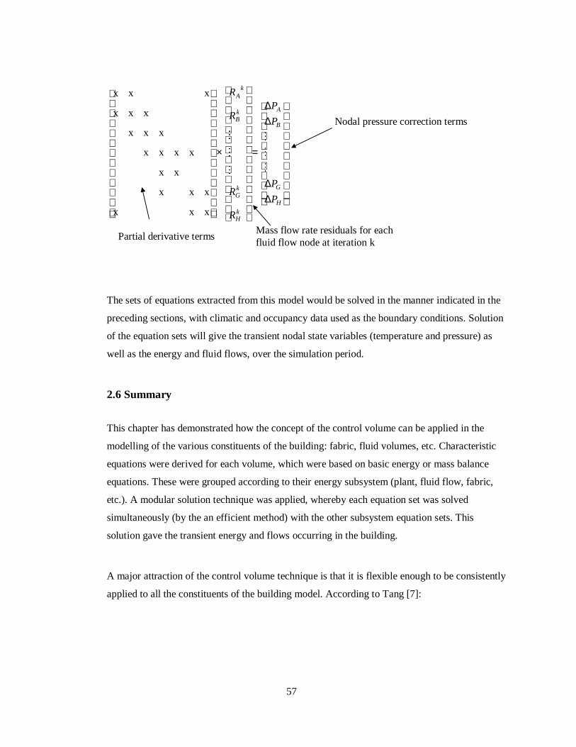
57
The sets of equations extracted from this model would be solved in the manner indicated in the
preceding sections, with climatic and occupancy data used as the boundary conditions. Solution
of the equation sets will give the transient nodal state variables (temperature and pressure) as
well as the energy and fluid flows, over the simulation period.
2.6 Summary
This chapter has demonstrated how the concept of the control volume can be applied in the
modelling of the various constituents of the building: fabric, fluid volumes, etc. Characteristic
equations were derived for each volume, which were based on basic energy or mass balance
equations. These were grouped according to their energy subsystem (plant, fluid flow, fabric,
etc.). A modular solution technique was applied, whereby each equation set was solved
simultaneously (by the an efficient method) with the other subsystem equation sets. This
solution gave the transient energy and flows occurring in the building.
A major attraction of the control volume technique is that it is flexible enough to be consistently
applied to all the constituents of the building model. According to Tang [7]:
x x x
x x x
x x x
x x x x
x x
x x x
x x x
×
=
R
R
R
R
P
P
P
P
Ak
Bk
Gk
Hk
A
B
G
H
M
M
M
M
M
M
∆∆
∆∆
Nodal pressure correction terms
Mass flow rate residuals for eachfluid flow node at iteration k
Partial derivative terms

58
“… this technique has not only the ability to model complex boundary conditions, time-varying
parameters, multi-dimensional problems, but also has the potential of applying the methods of
modern control theory , leading to a higher level of modelling and development.”
In the next chapter the flexibility of the modelling techniques outlined in this chapter will be
demonstrated by their application to electrical networks.

59
2.7 References
1. Clarke J A, Development of a prototypical component-based energy modelling system, Final
Report for Grant GR/D/26610.
2. Clarke J A, Energy simulation in building design, Adam Hilger, Bristol, 1985.
3. Mitchell A R, Computational methods in partial differential equations, Wiley, New York,
1969.
4. Cockroft J P, Heat transfer and air flow in buildings, PhD thesis, University of Glasgow,
1979.
5. Negrao C O R, Conflation of Computational fluid dynamics with building energy simulation,
PhD Thesis, University of Strathclyde, Glasgow, 1995.
6. Clarke J A and Beausoleil-Morrison I, The integration of Computational Fluid Dynamics
into building simulation, IBPSA News, Vol. 9, No. 2, Dec 1997.
7. Tang D, Modelling of heating and air-conditioning system, PhD Thesis, University of
Strathclyde, 1985.
8. Aasem E O, Practical simulation of buildings and air-conditioning systems in the transient
domain, PhD Thesis, University of Strathclyde, Glasgow 1993.
9. Hensen J L M, ESPmfs, a building and plant mass flow network solver, Collaborative
FAGO/ESRU report 90.14K, 1990.
10. McLean D, Simulation of solar energy systems, PhD Thesis, University of Strathclyde, 1982.

60
11. Chow TT, Clarke J A and Dunn A, Primitive parts: an approach to air-conditioning
component modelling, Energy and Buildings No. 26, 1997.
12. Walton G, A computer algorithm for predicting infiltration and inter-room air flows,
ASHRAE Transactions, 1990, Part 1.
13. Clarke J A and Hensen J L M, Implementation of a new air flow equation solver in ESP,
ESRU Technical Report, University of Strathclyde, 1988.
14. Nakhi A E, Adaptive construction modelling within whole building dynamic simulation, PhD
Thesis, University of Strathclyde, Glasgow, 1995.
2.8 Bibliography
Clarke J A, Energy Simulation in Building Design, Adam Hilger, Bristol, 1985.
Hensen J L M, On the thermal interaction of building structure and heating and ventilation
system, PhD. Thesis, Eindhoven University of Technology, 1991.

61
Chapter 3 - Modelling the Electrical Network
3. Introduction
In the previous chapter the concept of modelling the building using characteristic control
volumes was introduced. These were used to model the building fabric and associated networks
(plant, fluid flow etc.). However, one critical constituent of the building was not included: the
electrical energy subsystem. The ability to model this element of the building is vital if
simulation tools are to be used in the design, evaluation and optimisation of the building-
integrated energy systems outlined in chapter 1.
This chapter sets out to develop a means of modelling and simulating the electrical energy
subsystem as a component of an integrated building model, which incorporates all the important
energy and mass transport phenomena: heat transfer and storage in the fabric, infiltration, air and
vapour flows, heat transfer and fluid flows in the plant system, heat gains from occupants and
lighting, moisture migration and storage and electrical energy flows.
Addition of electrical energy flows to the building model requires that the concept of the control
volume, as described in chapter 2, is extended to the modelling of the building’s electrical
system. As with plant, fluid and moisture flow, the power system is modelled as a network,
constructed from a coupled set of electrical control volumes.
However, before describing the principles behind the modelling of the electrical system, it is
important to understand its key characteristics and function.
3.1 A Brief Overview of the Electrical System
Any electrical power system has three main constituents: loads, sources and a distribution
system. The loads are the end-points of the power system, consuming the electrical energy
supplied by the sources, which are either local generators or points where the power system

62
draws energy from a larger network such as the electricity supply grid. Transmitting the
electrical energy between these two are the cables, transmission lines and transformers which
make up the distribution system.
Thinking in terms of a building, the main electrical loads would consist of electric heaters, lights,
office equipment and the motors driving fans and pumps. Normally, a building will be powered
by a connection to the local grid, which can be considered as a source of electrical energy. When
considering building-integrated energy systems, the connection to the local electricity supply is
augmented or replaced by the building-integrated sources of power discussed in chapter 1:
façade-integrated photovoltaic arrays (PV) or small scale combined heat and power (CHP). The
cabling connecting the generators, local supply and the loads make up the building’s distribution
system.
The loads in a power system can be considered as the points of interaction between the thermal
and the electrical energy subsystems: electrical loads release heat into the building through the
degradation of the high grade electrical energy, also the electrically-powered motors in fans and
pumps circulate air and water throughout the building. In effect, the loads couple the thermal to
the electrical systems through the conversion of electrical to thermal energy, or by assisting in
the transport of thermal energy to the point of use.
In addition to interactions at the loads, the thermal and electrical energy subsystems can interact
at the points of energy production, e.g. a combined heat and power unit (CHP) will supply power
to the building’s electrical system, while at the same time providing hot water to the building
plant.
The modelling of the loads and sources that draw or provide electrical energy to this network is
the subject of chapter 5. This chapter is concerned with the modelling and solution of the
distribution system and its associated electrical energy flows.

63
3.2 Developing a Model of the Electrical System
Any model of a building’s electrical system must incorporate the fundamental characteristics
outlined in the previous paragraphs and also allow its simulation, in an integrated fashion, with
the rest of the building model. Towards this end, the same modelling techniques applied in
chapter 2 will be used here in the development of the electrical system model.
• The control volume principle will be extended to electrical systems, along with the
development of a corresponding characteristic equation.
• The concept of linking the control volumes to form a network, introduced in chapter 2, will
be used as the means of describing the electrical system.
• An equation set will be extracted from the control volumes for use in the solution of the
network.
• A solution technique will be introduced, suitable for integration into the modular
simultaneous solution process used by ESP-r.
3.2.1 The Control Volume Applied in an Electrical Context
The fundamental basis behind all the equations derived for the control volumes of chapter 2 was
the application of the laws of conservation of mass, energy and momentum. In the context of the
electrical energy subsystem, only one conservation law is relevant: the conservation of electrical
energy. This is achieved by the application of Kirchhoff’s current law, which stipulates that the
sum of phasor9 currents at any point in an electrical system is always zero. The application of
9 The concept of the phasor is explained in section 3.4.1.

64
this law in terms of a control volume10 is shown in figure 3.1 in which a fictitious boundary is
drawn around a point in an electrical system.
Figure 3.1 An electrical control volume.
For the control volume shown in figure 3.1 the basic balance equation is as follows
I i jj
n
, ==
∑ 01
. (3.1)
10 This chapter’s definition of the electrical control volume is intended to be as generic as possible: the
control volume modelling technique can be applied to both alternating current (a.c.) and direct current
(d.c.). The following examples illustrate the application to a.c. systems but section 3.4.3 details how it can
be applied to d.c. systems.
i
d
b
ce …
n
a
I i,e
I i,d
I i,nI i,a
I i,b
…
control volumeboundary
conductor
electrical nodecurrentflow

65
n is the number of current flows associated with node i. Ii j, is the phasor of the current (A)
flowing between the control volume node i and some other connected node j. Note that the
current phasor is represented by a complex number of the form I x iy= + : the bar above the I
indicates a complex term.
Equation 3.1 can be further refined by classing each current associated with a control volume
into three categories [1]:
1. the current which is transmitted to other nodes;
2. the current which is absorbed by a load connected to the node;
3. the current which is injected into the node from a connected source.
The reason for the distinction is that currents flowing to loads and from sources are assumed to
be external to the network, and can therefore be regarded as boundary conditions. In order to
achieve a solution for the equations derived in this section these boundary conditions must be
known; this is discussed in section 3.3.1.
Equation 3.1 can therefore be re-written as
I I IT i aa
nT
Gi Lic
nL
b
nG
b c,= ==
∑ ∑∑+ − =1 11
0 . (3.2)
IT i aa
nT
,=
∑1
is the sum of currents transmitted to other nodes, IG ib
nG
b
=∑
1
is the sum of currents
injected into the node from a connected electrical energy source and −=
∑ I Lic
nL
c
1
is the sum of
currents absorbed by connected loads. Current flowing from the node is arbitrarily considered as

66
negative; this is the same convention as used ESP-r with the thermal and fluid flow subsystems.
Referring to equation 3.1, the number of transmitted, injected and absorbed currents is the same
as the n currents associated with the node: nT+ nG + nL = n.
Equation 3.2 is the basic balance equation, derived by the application of Kirchhoff’s current law,
for the electrical control volume.
3.2.2 Developing an Electrical Network
To illustrate the use of the electrical control volume in modelling an electrical system, consider
the following example; this consists of a series of electrical loads and sources connected by a
distribution system.
Figure 3.2 A simple electrical system.
To develop an electrical network model, electrical control volumes (represented by nodes) are
placed at critical points in the system. The critical points are the junctions of the electrical
conductors, as shown in figure 3.2. The connections between the nodes and loads are represented
L L L L L
L
L
junction ofconductors
load
generator
electricalconductor

67
by complex impedances (Ω), giving the network shown in figure 3.3. This network is an
equivalent circuit representation of the power system of figure 3.2.
Figure 3.3 The network representation of equation of a simple power system.
If the basic current balance equation 3.2 is applied to node a in the network the following
equation emerges.
I I I IT a b T a e G a La, ,+ + − = 0 . (3.3)
Placing the boundary terms (loads and generated currents) on the right hand side gives
I I I IT a b T a e G a L a, ,+ = − + . (3.4a)
Doing likewise for the other nodes in the network gives the following.
I I I IT T T L bb a b c b e, , ,+ + = ; (3.3b)
a b c
e
d
Za,e
Zc,dZa,b Zb,c
Zd,e
Zb,eZc,e
Za,b
a
ILaILb IGa ILc1
ILc2IGc ILd
ILe
node
impedance
load
source

68
I I I I I IT T T Gc Lc Lcc b c d c e, , ,+ + = − + +1 2 ; (3.3c)
I I IT T Ldd c d e, ,+ = ; (3.3d)
I I I I IT T T T Lee a e b e c e d, , , ,+ + + = . (3.3e)
3.2.3 Extracting the Equation Set
Equations 3.3a-e are the basic control volume current balance equations of the simple power
system of figure 3.2. Like the equations derived in chapter 2, they are based on the balance of a
flow variable such as heat flux, air or fluid flow. In this case the flow variable is electric current.
However, to solve the derived equations it will be necessary to convert them to the form seen in
all the characteristic equations of chapter 2 (e.g. equations 2.8, 2.13, 2.22 etc.). These equations
contain three types of variables: driving variables (e.g. temperature or pressure), resistance or
conductance (e.g. thermal resistance) and known boundary condition terms. The equations were
then solved for the driving variable: in an electrical network this is the voltage.
Equations 3.3a-e already contain the boundary terms in the form of the generated and load
currents. However, they will require some manipulation to introduce voltage and resistance
terms. This is achieved using Ohm’s law to replace the transmitted currents:
IV V
Zi ji j
i j,
,
=−
. (3.5)
Vi and Vj are the voltages (V) at nodes i and j respectively, Zi j, is the impedance (Ω) of the
connection between them. The Zi j, term is derived from a small equivalent circuit model of a
line, cable or transformer which connects the two points i and j. The formulation of these circuit
models is described in chapter 5.

69
Substituting equation 3.5 into 3.4a gives an expression for the electrical energy balance at node a
in terms of a driving variable (the voltage), resistance (i.e. the impedance) and the boundary
variables IG a and I La :
aLaGea
ea
ba
ba IIZ
VV
Z
VV+−=
−+
−
,,
. (3.6)
Rearranging the equation for Va gives
( ), , , ,Y Y V Y V Y V I Ia b a e a a b b a e e G a La+ − − = − + . (3.7)
The symbol Y is used in place of 1 / Z , where Y is the inverse of impedance, termed the
admittance (Ω-1).
Similar equations can be derived for all the other nodes in the network:
− + + + − − =Y V Y Y Y V Y V Y V Ia b a a b b c b e b b c c b e e Lb, , , , , ,( ) ; (3.6b)
− + + + − − = − + +Y V Y Y Y V Y V Y V I I Ib c b b c c d c e c c d d c e e Gc Lc Lc, , , , , ,( ) 1 2 ; (3.6c)
− + + − =Y V Y Y V Y V Ic d d c d d e d d e e Le, , , ,( ) ; (3.6d)
− − − − + + + + =Y V Y V Y V Y V Y Y Y Y V Ia e a b e b c e c d e d a e b e c e d e e Le, , , , , , , ,( ) . (3.6e)
The equations are now in a form similar to those developed in chapter 2: defined in terms of a
driving variable (Vi ), conductance ( Yi j, ) and boundary condition variables I G and I L .

70
The general form of equations 3.6a-e is
Y V Y V I Ix yy
z
x x yy
z
y Gt
u
Lv
w
xt
xv, ,
= = = =∑ ∑ ∑ ∑
− = − +
1 1 1 1, (3.8)
where z is the number of nodes in the network, u is the number of coupled electrical sources and
w is the number of coupled loads.
Hence, from the simple current balance associated with each electrical control volume, a set of
characteristic equations have been derived in terms of voltage, impedance (admittance) and
current flow. The equation set is linear and can be solved by direct methods for the set of
complex nodal voltages V :
V =
−
V
V
V
Vn
n
1
2
1
M .
3.2.4 Translation to Power Flow
While the derived set of equations offer a suitable means of determining the nodal voltages of
the network shown in figure 3.2, their solution is only achievable if the boundary conditions (the
electrical energy which is injected and drawn from the network) are defined in terms of current.
However, in the field of energy simulation, loads are typically defined in terms of a power
demand (W or VA). Similarly, the output of electrical sources would also be defined in terms of
power. It is therefore more appropriate to define the electrical network boundary conditions in
terms of power flow. Fortunately, the characteristic equations 3.6a-e are easily modified to
enable this is explained below.
Consider again the basic control volume current balance for node i (equation 3.2):
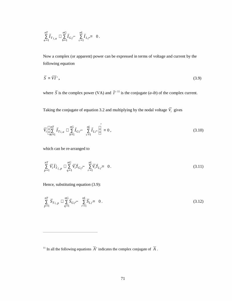
71
I I IT i aa
nT
Gi Lic
nL
b
nG
l m,= ==∑ ∑∑+ − =
1 110 .
Now a complex (or apparent) power can be expressed in terms of voltage and current by the
following equation
S VI= ′ , (3.9)
where S is the complex power (VA) and ′I 11 is the conjugate (a-ib) of the complex current.
Taking the conjugate of equation 3.2 and multiplying by the nodal voltage Vi gives
V I I Ii T i am
nT
Gi Lic
nL
b
nGl m,
= ==∑ ∑∑+ −
′=
1 110 , (3.10)
which can be re-arranged to
V I V I V Ii T i pp
nT
i Gi i Lir
nL
q
nG
q r′ + ′ − ′ == ==
∑ ∑∑,
1 110 . (3.11)
Hence, substituting equation (3.9):
S S ST i pp
nT
Gi Lir
nL
q
nGq r,
= ==∑ ∑∑+ − =
1 110 . (3.12)
11 In all the following equations ′A indicates the complex conjugate of A .

72
ST a bp
nT
,=
∑1
is the complex power transmitted between the node i and connected nodes, SGiq
nG
q
=∑
1
is
the complex power injected at node i and SLir
nL
r
=∑
1
is the complex power drawn from the node by
a load.
Further, complex power can be decomposed into its real and imaginary parts such that
S P iQ= + , (3.13)
where P is the real power part (W) and Q is the imaginary power part (VAR). Splitting
equation 3.12 into real and imaginary parts gives
P P PT i pp
nT
Gi Lir
nL
q
nGq r,
= ==∑ ∑∑+ − =
1 110 ; (3.14a)
and
Q Q QT i pp
nT
Gi Lir
nL
q
nGq r,
= ==∑ ∑∑+ − =
1 110 . (3.14b)
The subscripts have the same meaning as before.
Hence, from the current balance equation 3.2, three power balance equations have been derived:
one each for complex, real and reactive power.
Returning to the network of figure 3.3, its characteristic equations can be re-written with the
boundary variables expressed in terms of complex power. Consider again the current balance
equation for node a,

73
I I I IT a b T a e G a L a, ,+ = − + .
Taking its conjugate and multiplying by the nodal voltage:
V I I V I Ia T a b T a e a G a L a( ) ( ), ,+ ′ = − + ′ . (3.15)
Using Ohm’s law the transmitted currents can be expressed in terms of nodal voltages and
impedance (see equation 3.5).
VV V
Z
V V
ZV I Ia
a b
a b
a e
a ea G a L a
− + −
′= − + ′
, ,
( ) . (3.16)
Writing the right-hand-side of the equation in terms of power flow and replacing the impedance
terms with admittance gives
( ) aLaGeaeababaa SSYVVYVVV +−=′−+− ,, )()( . (3.17)
Re-arranging the equation for Va :
( ) ( ) aLaGaeaebabaeaabaa SSVYVYVVYVYV +−=′′+′′−′′+′′ ,,,, . (3.18a)
This is the basic form of the power balance at node a. The left hand side of the equation
represents the power transmitted to connected nodes in terms of the voltage and impedance
(admittance). The right hand side of the equation contains the boundary terms expressed as
complex power flows. Note that as a result of the conversion from current flow to power flow
the balance equation is now non-linear and will have to be solved iteratively. This is discussed in
section 3.3.
Equations of a similar form can be derived for all the other nodes in the network:

74
( ) ( ) bLbebecbcbaabebbcbbbab SVYVYVYVVYVYVYV =′′+′′+′′−′′+′′+′′ ,,,,,, ; (3.18b)
( ) ( ) 21,,,,,, cLcLcGcecedcdcbbceccdcccbc SSSVYVYVYVVYVYVYV ++−=′′+′′+′′−′′+′′+′′ ; (3.18c)
( ) ( ) dLdededccdedddcd SVYVYVVYVYV =+′′+′′−′′+′′ ,,,, ; (3.18d)
( ) ( ) eLeeddeccebbeaaeedeeceebeeae SVYVYVYVYVVYVYVYVYV =′′+′′+′′+′′−′′+′′+′′+′′ ,,,,,,,, . (3.18e)
The general form of the power balance equation at any node i can be written as
∑∑∑∑====
+−=
′′−
′′
≠
z
r
rL
y
q
qGi
x
ppip
n
ppii ii
ip
SSVYVYV111
,1
, , (3.19)
where n is the number of nodes in the network, y is the number of connected sources and z is the
number of connected loads.
Equation 3.19 can be simplified by adding the bracketed summation terms on the left-hand-side
of the equation such that
∑∑∑===
+−=
′
z
rL
y
qGi
n
ppip r
iq
iSSVV
111,Y (3.20)
where ∑=
′=n
ppiii Y
1,,Y and Y , ,i p i pp i
Y≠
= − ′ .
Y ,i i is the short circuit driving port admittance of node i and Y ,i p is a transfer admittance between
node i and some node p [2].

75
Equation 3.20 is the basic power balance equation for any node in an electrical network. Notice
its similarity with the fluid flow equations of section 2.3.4 in that it is a non-linear equation
expressed in terms of a driving variable V . The electrical network equation set consists of the
variants of equation 3.20 derived for each node.
3.3 Solution of the Equation Set
As with the fluid flow equations, a Newton-Raphson iterative technique is employed, which
solves for the voltages at each node. Once the nodal voltages are solved all other network
unknowns (such as current and transmitted power) can be derived. The solution of the electrical
network equation set, using the Newton-Raphson technique and power terms as boundary
conditions, is described as a ‘load flow solution’ by Stagg and El-Abiad [2]. Gross [1] describes
the same solution technique but using a compact polar notation; this is adopted in the description
which follows.
The first step in the solution process requires that the general nodal equation 3.20 is split into its
real and reactive parts. To achieve this, the complex variables on the left-hand side of the
equation are expressed in polar form, e.g. for V :
V V i= +(cos sin )θ θ , (3.21a)
and
′ = −V V i(cos sin )θ θ . (3.21b)

76
where V is the modulus of V and θ is its argument. Applying De Moivre’s theorem12, equation
3.20 can be decomposed into the following real and imaginary components.
V V P Pi p i pp
n
i p i p Gq
y
Lr
z
iq
irY cos( ), ,
= = =∑ ∑ ∑− − = − +
1 1 1θ θ α , (3.22a)
and for the imaginary terms (dividing through by i):
V V Q Qi p i pp
n
i p i p Gq
y
Lr
z
iq
irY sin( ), ,
= = =∑ ∑ ∑− − = − +
1 1 1θ θ α . (3.22b)
In the previous equations )sin(cos iiii iVV θθ += , )sin(cos pppp iVV θθ −=′ and
)sin(cosYY ,,,, pipipipi i αα −=′ . Also, S P iQG i G i G i= + , and S P iQLi Li Li= + .
With equation 3.20 now split into real and reactive components each node i in an electrical
network has two non-linear characteristic equations: one describing the real power balance, the
other describing the reactive power balance. There are also two unknowns: Vi and θi. Hence, an n
node electrical network would create 2n non-linear characteristic equations in 2n unknowns.
The Newton-Raphson solution method used with the fluid flow network is now applied in the
solution of the electrical network. Recall that the basis for the fluid flow solution was a Taylor’s
series expansion of a function f x x x xi i n( , , , ),1 2 0K K = about some known set of values xk,
where x x x xkn
k= ( , , , )1 2 K . In the case of the fluid flow equations, the function described the
12 De Moivre’s theorem (from [3]):
)sin()cos()sin(cos)sin)(cossin(cos 21212221 nnnn iiii θθθθθθθθθθθθ KKK +++++=+++

77
flow balance equation at each node i in the network and the function unknowns were the nodal
pressures differences ∆pi,j. Two functions of a similar form can be derived at each node i in the
electrical network; this is achieved by re-arranging equations 3.21a and 3.21b, and moving the
known terms to the left-hand side as follows.
0)cos(Y11
,1
, =−+−− ∑∑∑===
z
rL
y
qGpipi
n
ppspi r
iq
iPPVV αθθ (3.23a)
and
0)sin(Y11
,1
, =−+−− ∑∑∑===
z
rL
y
qGpipi
n
ppspi r
iq
iQQVV αθθ . (3.23b)
These two equations can be characterised by the functions which follow.
The real power balance:
0),,,,,,,,,( 2121 =ninii VVVVf θθθθ KKKK , (3.24a)
and the reactive power balance equation:
0),,,,,,,,,( 2121 =ninii VVVVg θθθθ KKKK . (3.24b)
In the following equations these functions will be abbreviated to fi(V,θ) and gi(V,θ), where
V=(V1,V2,…,Vn) and θ=(θ1,θ2,…,θn). Note that the function for the fluid flow equations involved
only one type of variable (the nodal pressures Pn), while both the electrical power balance
equations are functions with two types of variables: Vi and θi. Taylor’s series can be extended to
deal with this. Consider the expansion for the function fi(V,θ) for an unknown set of values Vk+ 1
and θk+ 1 about the known set of values Vk and θk.

78
KK
K
KK
M
KK
K
K
+∆+∆++∆+∆+
∆+∆++∆+∆+
∆+∆++∆+∆+
+∆+∆++∆+∆+
∆+∆++∆+∆+
∆+∆++∆+∆+
=
−
−
−
−
−
−
++
33
33
31
33
32
33
31
3
22
22
21
22
22
22
21
2
121
33
33
31
33
32
33
31
3
22
22
21
22
22
22
21
2
121
11
),(),(),(),(
),(),(),(),(
),(),(),(),(
),(),(),(),(
),(),(),(),(
),(),(),(),(),(
),(
in
kki
in
kki
i
kki
i
kki
in
kki
in
kki
i
kki
i
kki
in
kki
in
kki
i
kki
i
kki
in
kki
in
kki
i
kki
i
kki
in
kki
in
kki
i
kki
i
kki
in
kki
in
kki
i
kki
i
kkikk
i
kki
VVf
VVfVfVf
VfVfVfVf
VfVfVfVf
VV
VfV
V
VfV
V
VfV
V
Vf
VV
VfV
V
VfV
V
VfV
V
Vf
VV
VfV
V
VfV
V
VfV
V
VfVf
Vf
∂θθ∂
∂θθ∂θ
∂θθ∂θ
∂θθ∂
θ∂θ
θ∂θ∂θ
θ∂θ∂θ
θ∂θ∂θ
θ∂
θ∂θ
θ∂θ
∂θθ∂
θ∂θ
θ∂θ
∂θθ∂
∂θ∂
∂θ∂
∂θ∂
∂θ∂
∂θ∂
∂θ∂
∂θ∂
∂θ∂
∂θ∂
∂θ∂
∂θ∂
∂θ∂θ
θ
(3.25)
Re-arranging and truncating all terms of second order and above, the following expression
emerges:
.),(),(),(),(
),(),(),(),(
),(),(
121
121
11
in
kki
n
kki
kki
kki
in
kki
n
kki
kki
kki
kki
kki
VfVfVfVf
VV
Vf
V
Vf
V
Vf
V
Vf
VfVf
θ∂θ
θ∂∂θ
θ∂∂θ
θ∂∂θ
θ∂
∂θ∂
∂θ∂
∂θ∂
∂θ∂
θθ
∆
+++++
∆
++++
=−
−
−
++
K
K (3.26)

79
Applying the same technique to all the nodes in a network gives the following equation set for
the real power flow f(V,θ) function at each node.
;),(),(),(),(
),(),(),(),(
),(),(
11
1
1
2
1
1
1
11
1
1
2
1
1
1
111
1
θ∂θ
θ∂∂θ
θ∂∂θ
θ∂∂θ
θ∂
∂θ∂
∂θ∂
∂θ∂
∂θ∂
θθ
∆
+++++
∆
++++=
−
−
−
++
n
kk
n
kkkkkk
n
kk
n
kkkkkk
kkkk
VfVfVfVf
VV
Vf
V
Vf
V
Vf
V
Vf
VfVf
K
K
M
K
K
;),(),(),(),(
),(),(),(),(
),(),(
22
1
2
2
2
1
2
22
1
2
2
2
1
2
211
2
θ∂θ
θ∂∂θ
θ∂∂θ
θ∂∂θ
θ∂
∂θ∂
∂θ∂
∂θ∂
∂θ∂
θθ
∆
+++++
∆
++++=
−
−
−
++
n
kk
n
kkkkkk
n
kk
n
kkkkkk
kkkk
VfVfVfVf
VV
Vf
V
Vf
V
Vf
V
Vf
VfVf
.),(),(),(),(
),(),(),(),(
),(),(
121
121
11
nn
kkn
n
kkn
kkn
kkn
nn
kkn
n
kkn
kkn
kkn
kkn
kkn
VfVfVfVf
VV
Vf
V
Vf
V
Vf
V
Vf
VfVf
θ∂θ
θ∂∂θ
θ∂∂θ
θ∂∂θ
θ∂
∂θ∂
∂θ∂
∂θ∂
∂θ∂
θθ
∆
+++++
∆
++++=
−
−
−
++
K
K

80
An equation set of exactly the same form can be extracted for the reactive power flow function
g(V,θ); the general form of which, for any node i is
.),(),(),(),(
),(),(),(),(
),(),(
121
121
11
in
kki
n
kki
kki
kki
in
kki
n
kki
kki
kki
kki
kki
VgVgVgVg
VV
Vg
V
Vg
V
Vg
V
Vg
VgVg
θ∂θ
θ∂∂θ
θ∂∂θ
θ∂∂θ
θ∂
∂θ∂
∂θ∂
∂θ∂
∂θ∂
θθ
∆
+++++
∆
++++=
−
−
−
++
K
K (3.27)
As with the expression for real power flow, this equation is applicable to all n nodes in a
network.
Grouping the equations together in matrix form gives the following general expression for an n
node network.
∆
∆∆
∆
=
∆
∆
∆
∆
2
1
2
1
1
1
),(
1
),(),(
1
),(
),(1
1
),(1),(1
1
),(1
),(
1
),(),(
1
),(
),(1
1
),(1),(1
1
),(1
),(
),(
),(
),(
θ
θ
∂θθ∂
∂θθ∂
∂θ∂
∂θ∂
∂θθ∂
∂θθ∂
∂θ∂
∂θ∂
∂θθ∂
∂θθ∂
∂θ∂
∂θ∂
∂θθ∂
∂θθ∂
∂θ∂
∂θ∂
θ
θ
θ
θ
M
M
LL
MOMMOM
LL
LL
MOMMOM
LL
M
M
V
V
n
VngVng
nV
Vng
V
Vng
n
VgVg
nV
Vg
V
Vgn
VnfVnf
nV
Vnf
V
Vnf
n
VfVf
nV
Vf
V
Vf
Vg
Vg
Vf
Vf
kkkkkkkk
kkkkkkkk
kkkkkkkk
kkkkkkkk
kkn
kk
kkn
kk
(3.28)
In equation 3.28 ∆fi(Vk,θk) represents ∆fi(V
k+1,θk+1) - ∆fi(Vk,θk) and likewise ∆gi(V,θ) represents
∆gi(Vk+1,θk+1) - ∆gi(V
k,θk). The matrix on the left-hand side of equation 3.28 can be simplified as

81
the solution of the equation set requires that fi(Vk+1,θk+1) = 0 and gi(V
k+1,θk+1) = 0 for all nodes
in the system. The terms in the left-hand matrix therefore reduce to -∆fi (Vk,θk) and -∆gi (V
k,θk).
∆
∆∆
∆
=
−
−
−
−
2
1
2
1
1
1
),(
1
),(),(
1
),(
),(1
1
),(1),(1
1
),(1
),(
1
),(),(
1
),(
),(1
1
),(1),(1
1
),(1
),(
),(
),(
),(
θ
θ
∂θθ∂
∂θθ∂
∂θ∂
∂θ∂
∂θθ∂
∂θθ∂
∂θ∂
∂θ∂
∂θθ∂
∂θθ∂
∂θ∂
∂θ∂
∂θθ∂
∂θθ∂
∂θ∂
∂θ∂
θ
θ
θ
θ
M
M
LL
MOMMOM
LL
LL
MOMMOM
LL
M
M
V
V
n
VngVng
nV
Vng
V
Vng
n
VgVg
nV
Vg
V
Vgn
VnfVnf
nV
Vnf
V
Vnf
n
VfVf
nV
Vf
V
Vf
Vg
Vg
Vf
Vf
kkkkkkkk
kkkkkkkk
kkkkkkkk
kkkkkkkk
kkn
kk
kkn
kk
(3.29)
Equation 3.29 can be condensed to the following form
∆∆
=
θ∂θ∂∂∂
∂θ∂∂∂ V
JJ
JJ
R
R
gVg
fVf
Q
P
//
// . (3.30)
Rp represents the column matrix of real power residuals (equivalent to the mass flow residuals in
a fluid flow simulation), RQ represents the column matrix of reactive power residuals:
.
),(
),(
),(
,
),(
),(
),(
2
1
2
1
−
−−
=
−
−−
=
kkn
kk
kk
Q
kkn
kk
kk
P
Vg
Vg
Vg
R
Vf
Vf
Vf
R
θ
θθ
θ
θθ
MM
∆V and ∆θ are column matrices representing the difference in the modulus and arguments,
respectively, of the known variable set (Vk,θk)and the unknown variable set (Vk+1, θk+1)
(equivalent to the pressure correction vector in a fluid flow simulation):

82
∆
∆∆
=∆
∆
∆∆
=∆
nnV
V
V
V
θ
θθ
θMM
2
1
2
1
, .
In equation 3.30 the Jacobian matrix contains four terms which represent four groups, or sub-
matrices of partial derivatives present within in it:
.,1,),(
,),(
,),(
,),(
niVg
JV
VgJ
VfJ
V
VfJ i
gi
V
gi
fi
V
f K=====∂θ
θ∂∂
θ∂∂θ
θ∂∂
θ∂
∂θ∂
∂∂
∂θ∂
∂∂
The coefficients of these groups comprise of eight basic forms: the diagonal terms of each group
i
i
i
i
i
i
i
i Vg
V
VgVf
V
Vf
∂θθ∂
∂θ∂
∂θθ∂
∂θ∂ ),(
,),(
,),(
,),(
and the off-diagonal terms
ijnjVg
V
VgVf
V
Vf
j
i
j
i
j
i
j
i ≠= ,1),(
,),(
,),(
,),(
K
∂θθ∂
∂θ∂
∂θθ∂
∂θ∂
. These forms are created from
the partial derivatives of equation 3.23a and 3.23b calculated with a known set of nodal voltages
V k . They are defined as follows [1].
)(cosY)cos(Y),(
,1
, jiji
n
jjijiiiii
i
i VVV
Vf αθθα∂
θ∂−−+= ∑
=; (3.31a)
ijVVVf
jiji
n
jjiji
i
i ≠−−−= ∑=
)(cosY),(
,1
, αθθ∂θ
θ∂ (3.31b)
)(sinY)sin(Y),(
,1
, jiji
n
jjijiiiii
i
i VVV
Vg αθθα∂
θ∂−−+−= ∑
=; (3.31c)

83
ijVVVg
jiji
n
jjiji
i
i ≠−−= ∑=
)(cosY),(
,1
, αθθ∂θ
θ∂; (3.31d)
ijVV
Vfjijiiji
j
i ≠−−= )cos(Y),(
,αθθ∂
θ∂; (3.31e)
ijVVVf
jijiijjij
i ≠−−= )cos(Y),(
,αθθ∂θ
θ∂; (3.31f)
ijVV
Vgjijiiji
j
i ≠−−= )sin(Y),(
,αθθ∂
θ∂; (3.31g)
ijVVVf
jijiijjij
i ≠−−−= )sin(Y),(
,αθθ∂θ
θ∂; (3.31h)
Equation 3.30 forms the basis for the iterative solution of the network characteristic equations.
Solution of this equation, for the known set of nodal voltages (Vk,θk) by LU decomposition (see
section 2.3.4) gives the voltage modulus and argument correction factors. These are added to the
known voltages to give the voltage values for the next iteration:
∆∆
+
=
+
+
θθθVVV
k
k
k
k
1
1
, (3.32)
As equation 3.32 converges on a solution for the nodal voltages, the column matrix of nodal real
and reactive power flow residual terms (RPk and RQ
k) will tend towards zero. An ideal solution
would give a real and reactive power balance at each node:
R f V V V V V P Pp i n n i p s pp
n
i p i p Gq
y
Lr
z
i iq
ir= − = − − − + − =
= = =∑ ∑ ∑( , , , , , , , ) Y cos( ), ,1 2 1 2
1 1 1
0K Kθ θ θ θ θ α ,

84
and
R g V V V V V Q QQ i n n i p s pp
n
i p i p Gq
y
Lr
z
i iq
ir= − = − − − + − =
= = =∑ ∑ ∑( , , , , , , , ) Y sin( ), ,1 2 1 2
1 1 1
0K Kθ θ θ θ θ α .
Consequently, as the solution is approached, the corrections applied to the modulus and
arguments of the nodal voltage corrections will also tend towards zero. An approximate solution
for the electrical network voltages is obtained if the iterative process is halted when these
corrections fall below some user defined convergence value (i.e. ∆Vi<0.0001Vik and
∆θi<0.0001θik, i=1…n).
Once the approximate solutions are obtained for Vi and θi at each node i, the complex nodal
voltages can be obtained by substituting these values into equation 3.21a
Summarising: the solution method described here will solve the nodal voltages in an electrical
network, which comprises of a coupled set of electrical control volumes. Solution of the power
flows in the network requires that two non-linear balance equations are derived for each control
volume; these are solved simultaneously using a Newton-Raphson iterative technique. This
solution method is the same as that applied within ESP-r to the fluid flow network
It is possible to derive all the other network flow terms: transmitted current and transmitted
power, using the solved voltages and the known impedance characteristics of the network.
Recall that the current flowing between two control volumes, i and j, was given by equation 3.5
ji
jiji Z
VVI
,,
−=
The complex power flowing between the same two volumes is given by the application of
equation 3.9:

85
′
−=′=
ji
jiijiiji
Z
VVVIVS
,,, )( . (3.33)
3.3.1 Requirements for the Network Solution
The basic power balance equations for an the electrical control volumes (3.23a and 3.23b)
contain terms relating to the complex nodal voltage, the impedance characteristics of the
connections between the nodes and also to the power injected into and drawn from the node by
loads and sources respectively. Solution of the equation set dictates that, with 2n network
equations, there can be a maximum of 2n unknowns. The previous section showed how the
network can be solved with the complex voltage argument V, and modulus θ, as the unknowns.
It therefore follows that the other variables in the power flow equations: the impedance
characteristics of the network connections and the power drawn from and injected into each
node, must be known quantities.
The impedance characteristics of the network are in fact those of the components that connect
the various control volumes together. In a typical building these components would be the lines,
cables and transformers that make up the distribution system; the modelling of these network
constituents, and the derivation of their impedance characteristics is dealt with in chapter 5.
The real and reactive power flow boundary conditions (the power drawn from and injected into
each node in the network) are the major linkage points between the thermal model, described in
chapter 2, and the electrical network model. It is the task of the thermal element of the building
model to provide this power flow information (e.g. electric lighting loads, fan and pump power
consumption, electric heating loads, photovoltaic array output, etc.). In order for the building
model to provide this array of information a process of integration and model development must
be undertaken; this is described in chapters 4 and 5 respectively.
The final pre-requisite for solution of the electrical network is that at least one of the nodal
voltages in the network is known: this value acts as a reference for the iterative solution. If no

86
nodal voltage were known, then an infinite number of network voltage states would satisfy the
requirements of a network solution. This situation happens because the nodal power flows are
driven by a voltage difference. Hence, as long as the nodal voltage differences are the same, any
number of permutations of nodal voltage values would satisfy the requirements for real and
reactive power balance at each node. The use of a known value ensures that only one set of
nodal voltages gives the correct solution. The known value in the network is usually taken as the
point where the main power source connects to the network. That power source can either be a
generator or the connection to the local supply grid. The node connected to the power source
will then take the voltage of the supplying generator or the connected grid. Note that the known
voltage value need not be constant, but can change throughout the simulation (but not during the
iterative solution). This opens up the possibility for voltage time series data (i.e. real grid voltage
data) to be used as a boundary condition for the network solution.
The starting point for the iterative solution process is some initial set of voltages V k . These can
be provided through a guess, or more conveniently, the set of voltages from a previously solved
system state, which in the context of a building simulation can be the network voltages that were
calculated at the previous time step.
3.4 Application to Typical Building Electrical Systems
The previous sections have detailed a generic means of describing and solving an electrical
system. However, to be useful, this solution method must be flexible enough to be applied to the
types of systems found in buildings, these are: three-phase a.c., single-phase a.c. and d.c.
systems. The network approach to modelling the electrical system relies on it being modelled as
an equivalent circuit, with the circuit state variables described as phasor quantities. Hence, to
model any particular electrical system it is necessary to represent it in that particular form. How
this is done for the three system types mentioned above is outlined in the following sections.

87
3.4.1 Alternating Current and Phasor System Variables
The most common type of power system found in buildings involve alternating current (a.c.),
where both the supplied current and voltage vary sinusoidally with time, with an angular
frequency of ω radians per second. Under normal operating conditions the frequency is steady
and these two quantities can be characterised by the general equation:
)cos(A)( ϕω += tta (3.34)
Where a(t) is the sinusoidally varying quantity, A is its amplitude, ω is its angular frequency
(radians/s)and ϕ is the phase angle (radians) in relation to the time domain.
Real and reactive power, which are both derived from voltage and current terms, must therefore
also vary sinusoidally. So, for the a.c. power system, all the voltage and power-related quantities
used in the various balance equations of sections 3.2.2-3.2.4 can be characterised by this type of
function. However, the method of solution outlined in the previous section described the system
state variables as phasor quantities. This was done because at solution frequencies of
considerably longer than the time period of the sinusoidal oscillation (≈0.02s) the sub-second
fluctuations of voltage and current become unimportant. The solution frequency in energy
simulations usually ranges from hourly to sub-minutely calculations. Hence, in this case it is
acceptable to use the phasor value for the electrical system state variables: a phasor being an
entity that captures the time-averaged characteristics of a sinusoidally varying function and is
derived as follows.
Equation 3.34 can be re-written in the form:
)])sin()(Re[cos(A)( ϕωϕω +++= titta .
Applying De Moivre’s theorem and separating the time varying components gives
)])sin)(cossin(Re[(cosA)( ϕϕωω ititta ++= . (3.35)

88
If a(t) is analysed at a period longer than 2π/ω (the time period of the sinusoidal oscillation) then
the phasor value A is a more appropriate measure of the oscillating quantity. This requires that
the time varying component of a(t) is replaced with its root mean squared (r.m.s.) value (from
[4]):
2
A]sinRe[cos2/1
0
2
=
+∫=
=dt
T
titA
Tt
t
ωω . (3.36)
The phasor value is defined as:
)sin(cos)sin(cos2
A ϕϕϕϕ iAiA +=+= . (3.37)
The phasor contains the vital information of the sinusoidal function: the magnitude and the
relation to the time domain (the phase angle). Provided the system frequency is known, the
original sinusoidal function can be reconstructed from the phasor value:
)]sin)(cosRe[(2)( titAta ωω += . (3.38)
However, this reverse transformation is not required for the purposes of an energy simulation as
the phasor quantity contains all the information necessary for the calculation of the system
power flows.
3.4.2 Three Phase and Single Phase a.c. Systems
The power supplied to buildings is normally provided by three separate conductors, which
supply three separate phases of power. A fourth, grounded conductor, the neutral, acts as a return
path for the three-phase currents and as the reference for the other conductor voltages. Note that
in the analysis that follows the neutral conductor is not considered, the reasons for this are
explained in chapter 5, when the component models of the conductors (the connections between
the control volumes) are derived.

89
In the three conductors, the phase of power is determined by the relationship between the
sinusoidal variation of the voltage and current with the time domain; this is represented by the
phase angle ϕ. In three-phase systems the sinusoidal variations of both current and voltage
between each conductor are separated by 2π/3 radians, or 120o; the phasor representations of
these voltages and currents are as follows.
Conductor 1:
);sin(cos 1111 αα iVV += (3.39a)
);sin(cos 1111 ββ iII += (3.39b)
conductor 2:
));2/3sin()2/3(cos( 2222 παπα +++= iVV (3.40a)
));2/3sin()2/3(cos( 222 πβπβ +++= iII i (3.40b)
finally, for conductor 3:
));2/3sin()2/3(cos( 3333 παπα −+−= iVV (3.41a)
))2/3sin()2/3(cos( 333 πβπβ −+−= iII . (3.41b)
The three-phase power flow is given by

90
)).2/3sin()2/3))(cos(2/3sin()2/3(cos(
))2/3sin()2/3))(cos(2/3sin()2/3(cos(
)sin)(cossin(cos
333333
222222
111111
3322113
πβπβπαπα
πβπβπαπα
ββαα
−−−−+−+
+−+++++
−+=
′+′+′=−
iiIV
iiIV
iiIV
IVIVIVS ph
(3.42)
Applying de Moivre’s theorem gives
)].sin()[cos(
)]sin()[cos(
)]sin()[cos(
333333
222222
1111113
βαβα
βαβα
βαβα
−+−+
−+−+
−+−=−
iIV
iIV
iIVS ph
(3.43)
Note that the three-phase power is a function of the voltage and current magnitudes and the
phase angle between them. The 3π/2 phase differences disappear from the expression.
3.4.2.1 A Comprehensive Three-phase Analysis
The most direct means of analysis of a three-phase system involves the explicit representation of
each in a comprehensive network model. This task is made easier by the fact that three-phase
distribution systems are generally symmetrical, with each point in the network linked by three-
phase conductors, or three, separate single phase conductors. Note, three-phase conductors are
individual conductors which share a common path (e.g. encapsulated in a single cable) and share
a common neutral. The close proximity of the phase conductors creates electromagnetic (mutual)
couplings between them, this is explored further in chapter 5, and complicates the analysis of the
three-phase system. Separate single-phase conductors are generally not mutually coupled. Both
the three-phase and single-phase conductors are shown in figure 3.4. It should be noted that the
mutual couplings are the only interactions between the phases, which are essentially three
separate, symmetrical, circuits.

91
Given the inherent symmetry of the three-phase system, and the need to treat the power flows in
each phase independently, it is convenient to adapt the nodal schema to suit the nature of the
network. Recall that in the previous analyses a node was placed at each point in the system, this
can be extended to the three-phase case by placing a three-node array at each point of interest in
the system (e.g. conductor junctions), where each node relates to a phase. Considering a point i
in a network, the corresponding three-node array would be i1, i2 and i3; the subscript denotes the
phase of the node. Given the fact that each phase is a separate circuit, a node can only connect to
another node in the network if it shares the same subscript (i.e. phase) and consequently, the
subscript notation must remain consistent throughout the network. This is shown in figure 3.4.
Figure 3.4 A comprehensive three-phase network model.
All the equations derived previously can be applied in the analysis of the comprehensive three-
phase network. However, each point will have six energy balance equations (two for each node);
it is therefore convenient to express these equations in matrix form. Consider the characteristic
energy balances derived previously: in a comprehensive three-phase network their form would
be as follows.
a1
a2
a3
c1 c2 c3
d1 d2 d3
e1
e2
e3
xnyn
Zx,y=
b1 b2 b3
three-phasenodaltriplet
mutual couplingsbetween conductors
a three-phaseconductor
load
source
3 x 1 single-phaseconductors (notmutually coupled)

92
[ ] 0)cos(Y1
123
1
123
1
123,, =−+−− ∑∑∑
===
z
r
y
q
n
ppipipipi r
iLqiG
PPVV αθθ , (3.44a)
where n is the number of three-phase conductors connected to node i, y is the number of
connected sources and z is the number of connected loads.
=
ri
ri
ri
ri
L
L
L
L
P
P
P
P
3
2
1123 and
=
qi
qi
qi
qi
G
G
G
G
P
P
P
P
3
2
1123 .
The bracketed elements of equation 3.44a can be split into two groups: those in which i = p and
those in which i ≠ p. These are defined as follows.
[ ]
,)cos(Y00
0)cos(Y000)cos(Y
)cos(Y
333333
222222
111111
,
,
123,
ipVV
VVVV
VV
pi,pipi
pi,pipi
pi,pipi
pipii,ppi
=
=−−
φφ
φ
αθθ (3.44b)
where nnnnnn pipipi ,, αθθφ −−= ;
and
[ ]
.
)cos(Y00
0)cos(Y0
00)cos(Y
)cos(Y
333333
222222
111111
,
,
123
ip
VV
VV
VV
VV
,pipipi
,pi,pipi
pi,pipi
i,ppii,ppi
≠
=−−
φφ
φ
αθθ(3.44c)

93
When a three-phase conductor connects the points i and p, whose conductors are mutually
coupled, the elements of the bracketed term of equation 3.44a change to the following.
[ ]
.
)cos(Y)cos(Y)cos(Y
)cos(Y)cos(Y)cos(Y
)cos(Y)cos(Y)cos(Y
)cos(Y
333333,322,2,3233,311,1,3133
,2333,2333222222,211,1,2122
,1333,1333,1222,1221111111
,,,,
,,,,,
,,,,,,
123,,
ip
VVVVVV
VVVVVV
VVVVVV
VV
pipipimpimpimpimpi
mpimpipipipimpimpi
mpimpimpimpipipipi
pipipipi
pipipipi
pipipipi
pipipipi
=
=−−
φφφφφφφφφ
αθθ
(3.44d)
Where nnnnnpninn pipimpi ,
,,, αθθφ −−= and baxym
,Y is the mutual coupling between phases x and
y of the conductors linking points a and b. Note how the effect of the mutual couplings is to
introduce off-diagonal terms into the matrix, which act to couple together the equation set of the
three-node array.
The elements where p ≠ i are given by
[ ]
.
)cos(Y)cos(Y)cos(Y
)cos(Y)cos(Y)cos(Y
)cos(Y)cos(Y)cos(Y
)cos(Y
333333,322,2,3233,311,1,3133
,2333,2333222222,211,1,2122
,1333,1333,1222,1221111111
,,,,
,,,,
,,,,,,
123,,
ip
VVVVVV
VVVVVV
VVVVVV
VV
pipipimpimpimpimpi
mpimpipipipimpimpi
mpimpimpimpipipipi
pipipipi
pipipipi
pipipipi
pipipipi
≠
=−−′
φφφφφφφφφ
αθθ
(3.44e)
In all the preceding equations ∑=
=n
jjiii nnnn
Y1
,,Y and nnnn jiii Y ,,Y −= . Similarly
∑=
=n
jmm
iixyiixyY
1,,
Y and iixyiixy mm Y
,,Y −= .

94
Expressions for both the admittance terms of the form (nn baY , ) and mutual admittance terms
(baxymY
,) are given in chapter 5, when the three-phase conductor is discussed.
The equation set for the three-node array’s reactive power balance is of a similar form:
[ ] 0)sin(Y1
123
1
123
1
123,, =−+−− ∑∑∑
===
z
r
y
q
n
ppipipipi
riLq
iG
QQVV αθθ (3.44f)
The overall iterative equation for the solution of the three-phase equation set would be derived in
exactly the same way as described previously, though reflecting the triplicate nature of the three-
phase network model, this is shown over.

95
−−−
−−−−−−
−−−
f V
f V
f V
f V
f V
g V
g V
g V
g V
g V
g V
g V
k k
k k
k k
nk k
nk k
nk k
k k
k k
k k
nk k
nk k
nk k
1
1
1
1
1
1
1
2
3
1
2
3
1
2
3
1
2
3
( , )
( , )
( , )
( , )
( , )
( , )
( , )
( , )
( , )
( , )
( , )
( , )
θθθ
θθθθθθ
θθθ
M
M
=
∂ θ
∂
∂ θ
∂
∂ θ
∂
∂ θ
∂
∂ θ
∂
∂ θ
∂
∂ θ
∂θ
δ θ
∂θ
∂f V
V
f V
V
f V
V
f V
Vn
f V
Vn
f V
Vn
f V f V f Vk k k k k k k k k k k k k k k k k
1
1
1
1
1
1
1 1 1 1
1
1
1
11
1
1
2
1
3
1
1
1
2
1
3
1
1
1
2
1( , ) ( , ) ( , ) ( , ) ( , ) ( , ) ( , ) ( , ) ( , ) ( , ) ( , ) ( , )
( , ) ( , ) ( , ) ( , ) ( , ) ( , ) ( , )
θ
∂θ
∂ θ
∂θ
∂ θ
∂θ
∂ θ
∂θ
∂ θ
∂
∂ θ
∂
∂ θ
∂
∂ θ
∂
∂ θ
∂
∂ θ
∂
∂ θ
∂θ
k k k k k k k
k k k k k k k k k k k k k k
f V
n
f V
n
f V
nf V
V
f V
V
f V
V
f V
Vn
f V
Vn
f V
Vn
f V1
1 1 1
1
1
1
1
1
1
1 1 1 1
3
1
1
1
2
1
3
2
1
2
2
2
3
2
1
2
2
2
2
2
L
L
1
1
1
1
1
1 1 1
1
1
1
1
1
1
1 1 1
1
2
2
2
3
3
1
3
2
3
3
3
1
3
2
3
3
3
1
3
2
3
∂ θ
∂θ
∂ θ
∂θ
∂ θ
∂θ
∂ θ
∂θ
∂ θ
∂θ
∂ θ
∂
∂ θ
∂
∂ θ
∂
∂ θ
∂
∂ θ
∂
∂
f V f V f V
n
f V
n
f V
nf V
V
f V
V
f V
V
f V
Vn
f V
Vn
f V
k k k k k k k k k k
k k k k k k k k k k
( , ) ( , ) ( , ) ( , ) ( , )
( , ) ( , ) ( , ) ( , ) ( , ) ( k k k k k k k k k k k k k k
k k k k k k k
Vn
f V f V f V f V
n
f V
n
f V
n
fn V
V
fn V
V
fn V
V
fn V
, ) ( , ) ( , ) ( , ) ( , ) ( , ) ( , )
( , ) ( , ) ( , ) ( ,
θ
∂
∂ θ
∂θ
∂ θ
∂θ
∂ θ
∂θ
∂ θ
∂θ
∂ θ
∂θ
∂ θ
∂θ
∂ θ
∂
∂ θ
∂
∂ θ
∂
∂ θ
3
3
1
3
2
3
3
3
1
3
2
3
3
1
1
1
2
1
3
1
1
1
1
1
1
1
1 1 1
1 1 1
MM M
M
M M
k k k k k
k k k k k k k k k k k k
k k k k
n
fn V
n
fn V
nfn V
V
fn V
V
fn V
V
fn V
n
fn V
n
fn V
nfn V
V
fn V
V
) ( , ) ( , )
( , ) ( , ) ( , ) ( , ) ( , ) ( , )
( , ) ( , )
∂θ
∂ θ
∂θ
∂ θ
∂θ
∂ θ
∂
∂ θ
∂
∂ θ
∂
∂ θ
∂θ
∂ θ
∂θ
∂ θ
∂θ
∂ θ
∂
∂ θ
∂
1
1
2
1
3
2
1
2
2
2
3
2
1
2
2
2
3
3
1
3
1 1 1
1 1
L L L L
2
3
3
3
1
3
2
3
3
1
1
1
2
1
3
1
1
1
2
1
3
2
1
1
1
1
1
1
1
1 1 1
1
∂ θ
∂
∂ θ
∂θ
∂ θ
∂θ
∂ θ
∂θ
∂ θ
∂
∂ θ
∂
∂ θ
∂
∂ θ
∂θ
∂ θ
∂θ
∂ θ
∂θ
∂
fn V
V
fn V
n
fn V
n
fn V
ng V
V
g V
V
g V
V
g V
n
g V
n
g V
ng
k k k k k k k k
k k k k k k k k k k k k
( , ) ( , ) ( , ) ( , )
( , ) ( , ) ( , ) ( , ) ( , ) ( , )
(
O
O
O
V
V
g V
V
g V
V
g V
n
g V
n
g V
ng V
V
g V
V
g V
V
g V
n
g V
k k k k k k k k k k k k
k k k k k k k k
, ) ( , ) ( , ) ( , ) ( , ) ( , )
( , ) ( , ) ( , ) ( , ) (
θ
∂
∂ θ
∂
∂ θ
∂
∂ θ
∂θ
∂ θ
∂θ
∂ θ
∂θ
∂ θ
∂
∂ θ
∂
∂ θ
∂
∂ θ
∂θ
∂1
1
1
1
1
1 1 1
1
1
1
1
1
1
1 1
1
2
2
2
2
2
1
2
2
2
3
3
3
3
3
3
3
1
1
1
L L L L
M M
k k k k
k k k k k k k k k k k k k k k k k k
n
g V
n
gn V
V
gn V
V
gn V
V
gn V
n
gn V
Vn
gn V
Vn
g V
n
g V
n
g V
, ) ( , )
( , ) ( , ) ( , ) ( , ) ( , ) ( , ) ( , ) ( , ) ( ,
θ
∂θ
∂ θ
∂θ
∂ θ
∂
∂ θ
∂
∂ θ
∂
∂ θ
∂
∂ θ
∂
∂ θ
∂
∂ θ
∂θ
∂ θ
∂θ
∂ θ
2
3
3
1
1
1
2
1
3
1
1
1
2
1
3
1
1
1
2
1
1
1 1 1
1 1 1
M M M M
) ( , ) ( , ) ( , )
( , ) ( , ) ( , ) ( , ) ( , ) ( , ) ( , )
∂θ
∂ θ
∂θ
∂ θ
∂θ
∂ θ
∂θ
∂ θ
∂
∂ θ
∂
∂ θ
∂
∂ θ
∂
∂ θ
∂
∂ θ
∂
∂ θ
∂θ
∂n
gn V
n
gn V
n
gn V
ngn V
V
gn V
V
gn V
V
gn V
Vn
gn V
Vn
gn V
Vn
g V
n
g
k k k k k k
k k k k k k k k k k k k k k3
1
1
1
1
1
1
2
1
2
2
2
3
2
1
2
2
2
3
2
11 1 1
1L
1 1
1 1 1
2
2
2
3
2
1
2
2
2
3
3
1
3
2
3
2
3
1
3
2
3
( , ) ( , ) ( , ) ( , ) ( , )
( , ) ( , ) ( , ) ( , ) ( , ) ( ,
V
n
g V
n
gn V
n
gn V
n
gn V
ngn V
V
gn V
V
gn V
V
gn V
Vn
gn V
Vn
gn V
k k k k k k k k k k
k k k k k k k k k k k
θ
∂θ
∂ θ
∂θ
∂ θ
∂θ
∂ θ
∂θ
∂ θ
∂θ
∂ θ
∂
∂ θ
∂
∂ θ
∂
∂ θ
∂
∂ θ
∂
∂ θ
L
k k k k k k k k k k k k k
Vn
g V
n
g V
n
g V
n
gn V
n
gn V
n
gn V
n
) ( , ) ( , ) ( , ) ( , ) ( , ) ( , )
∂
∂ θ
∂θ
∂ θ
∂θ
∂ θ
∂θ
∂ θ
∂θ
∂ θ
∂θ
∂ θ
∂θ3
3
1
3
2
3
3
3
1
3
2
3
3
1 1 1
∆∆∆
∆∆∆∆∆∆
∆∆∆
V
V
V
V
V
V
n
n
n
n
n
n
n
n
n
1
1
1
1
1
1
1
2
1
1
2
3
1
1
1
1
2
3
M
M
θθθ
θθθ

96
3.4.2.2 The Per-Phase Approach
Fortunately, the nature of three-phase systems often makes the complication of a comprehensive
model unnecessary as, in many cases, they operate in a balanced state. In this state the currents,
voltages and impedances in the each phase are of equal magnitudes, while the phase angle (α -
β) between voltage and current is the same in all three phases. In balanced conditions equation
3.43 can be re-written as
)]sin()[cos(33 βαβα −+−=− iVIS ph , (3.45)
where VI = V1I1 = V2I2 = V3I3 and (α - β) = (α1 - β1) = (α2 - β2) = (α3 - β3).
Equation 3.45 gives an important result: in a balanced state, the equations for power flow in each
phase are identical. It is therefore possible to solve for only one phase of the system and apply
the results to the other two, i.e. only one node needs to be used at each point of interest.
Equations 3.23a and 3.23b could therefore be used to characterise the energy balance at each
node. The balanced power flow boundary conditions can be scaled from three to the single phase
using a simple division by 3. As only one equivalent circuit of the balanced system is required,
the complexity of the network is greatly reduced. This means of analysis is termed ‘per-phase
analysis’.
However, where the three-phase system is not balanced, e.g. where one phase is heavily loaded,
the need for a comprehensive model is unavoidable.
3.4.2.3 Single Phase Systems
Smaller buildings will usually draw power from only one phase of a power supply, where the
power is supplied by only one conductor. In this case, as with the per-phase case, only one node
needs to be used at each point of interest in the system, and equations 3.23a and 3.23b would
characterise the energy balance at each node.
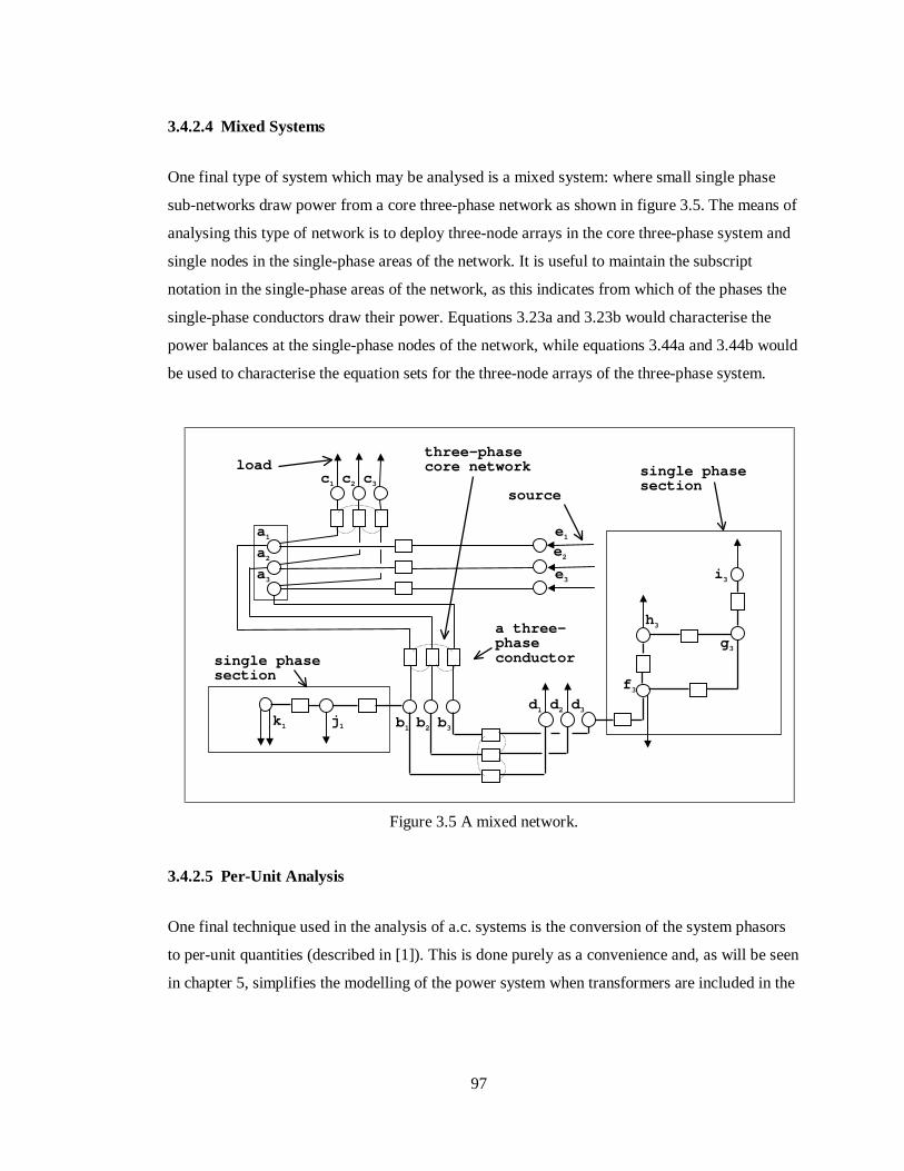
97
3.4.2.4 Mixed Systems
One final type of system which may be analysed is a mixed system: where small single phase
sub-networks draw power from a core three-phase network as shown in figure 3.5. The means of
analysing this type of network is to deploy three-node arrays in the core three-phase system and
single nodes in the single-phase areas of the network. It is useful to maintain the subscript
notation in the single-phase areas of the network, as this indicates from which of the phases the
single-phase conductors draw their power. Equations 3.23a and 3.23b would characterise the
power balances at the single-phase nodes of the network, while equations 3.44a and 3.44b would
be used to characterise the equation sets for the three-node arrays of the three-phase system.
Figure 3.5 A mixed network.
3.4.2.5 Per-Unit Analysis
One final technique used in the analysis of a.c. systems is the conversion of the system phasors
to per-unit quantities (described in [1]). This is done purely as a convenience and, as will be seen
in chapter 5, simplifies the modelling of the power system when transformers are included in the
d2 d3
a1
a2
a3
c1 c2 c3
d1
e1
e2
e3
b1 b2 b3
three-phasecore network
a three-phaseconductor
f3
g3
h3
i3
single phasesection
j1k1
single phasesection
load
source

98
network. The basis of conversion to per-unit is to chose two base magnitudes of system state
variables: usually voltage V and apparent power S. Division of these state variables by the
corresponding base value will give the per unit quantity. The base value for voltage is chosen so
that the resulting per unit value is close to unity. So for a 220V power system, the base value
chosen would be 220. At any particular node, where the voltage is V V i= +(cos sin )θ θ , the per
unit voltage is given by
VV
Vip u
base. . (cos sin )= +θ θ . (3.46)
The per-unit base values for impedance, admittance, real and reactive power can be easily
derived from the two original base values. Note that the per-unit parameters behave in exactly
the same way as the originals. Hence all basic circuit theories and equations also hold for per
unit parameters.
The other per unit values which are used with the power system are derived as follows.
IS
Vbasebase
base
= , (3.47)
ZV
Ibasebase
base
= , (3.48)
basebase Z
Y1= . (3.49)
3.4.3 d.c. Systems
The key difference between a.c. and d.c. systems is that the circuit state variables do not vary
sinusoidally. Hence, it is not necessary to translate the state variables to phasor form; they can be
represented by time averaged, real number values. Also not required in the d.c. circuit analysis
are any properties relating to reactive power flow. Hence all the imaginary components of the

99
state variables can be dispensed with. Considering the basic power balance equations 3.23a and
3.23b applied in a d.c. system analysis. Equation 3.23b is not relevant and equation 3.23a can be
written as
V V P Pi p i pp
n
Gq
y
Lr
z
iq
irC ,
= = =∑ ∑ ∑+ − =
1 1 1
0 . (3.50)
Vi represents a d.c. voltage at some node i in the system, while Vp is the d.c. voltage of the
connected node p. Ci,p is a conductance between nodes i and p (Ω-1): the conductance is the
inverse of this connection’s resistance (Ω). The conductance terms of equation 3.50 are
constructed in the same way as the admittance terms of equations 3.23a and 3.23b:
C , ,i i i pp
x
C==
∑1
and C , ,i p i pC= − . (3.51)
Finally, PG is a real power flow injected into the node from a source, while PL is a real power
flow drawn from the node by a load. Note that all the variables of the non-linear equations are
now real numbers.
Turning to the solution of the d.c. power flow network, the problem has now reduced from 2n
equations in 2n unknowns, for the a.c. case, to n equations of type f(V1,V2,…Vn) in n unknowns.
The unknowns are the d.c. voltage at each node. Hence, for a system of n nodes, the following
set of equations would emerge.
f V V V
f V V V
f V V V
n
n
n n
1 1 2
2 1 2
1 2
( , , , )
( , , , )
( , , , )
K
K
M
K

100
Application of Taylor’s series about a known set of network d.c. voltages Vk , as was done in the
a.c. solution, would eventually lead to the following equation:
−−
−
=
f Vf V
f V
f V k
V
f V k
Vn
fn V k
V
fn V k
Vn
V
V
V
k
k
nk
n
1
2
1
2
1
1
1
1
( )( )
( )
( ) ( )
( ) ( )M
L
M O M
L
M
∂
∂
∂
∂
∂
∂
∂
∂
∆∆
∆
. (3.52)
Equation 3.52 can be re-written as
[ ] [ ]R J Vpk
f
V
=
∂∂
∆ . (3.53)
Rpk represents a column matrix of real power residuals; these are determined from the application
of equation 3.23a at each node in the network. J f
V
∂∂
is the matrix of partial differentials, while ∆V
are the corrections to apply to the d.c. voltage at each node to obtain the value at iteration k+1;
these are obtained by solution of equation 3.52 LU decomposition.
The voltages for the next iteration of the d.c. network solution are therefore given by
[ ] [ ] [ ]V V Vk k+ = +1 ∆ . (3.54)
The same requirements for a solution apply to the d.c. network as applied to the a.c. case: all
power flow boundary conditions must be known along with at least one nodal voltage.

101
3.5 Application of the Technique to an Exemplar
The techniques outlined in this chapter for the modelling and solution of electrical systems will
now be applied to the simple exemplar introduced in chapter 2, through the addition of a simple
electrical system to the building model.
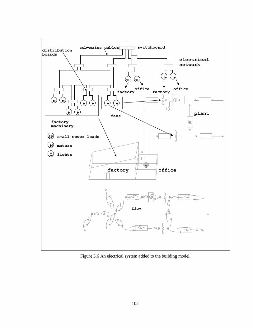
102
Figure 3.6 An electrical system added to the building model.
T
M M
M MM MM M
L LSP SP
SP
M
L
small power loads
motors
lights
switchboard
fans
factorymachinery
sub-mains cables
electricalnetwork
factoryoffice
factoryoffice
distributionboards
officefactory
plant
flow

103
Figure 3.6 shows that the electrical network supplies power to several constituents of the model:
the fans in the plant networks, electric motors in machinery on the factory floor and the lighting
system and small power loads in both zones.
Examining the power system of figure 3.6 in isolation, it can be seen that the building power
system is hierarchical: the main supply is brought in via one cable at the switchboard and
distributed to the loads by sub-mains cables. The system is three-phase, with power delivered to
the building at a line to neutral voltage of Vs. The motors in the factory and plant network draw
power from all three phases of the supply, while each lighting and small power load draws its
power from only one phase. The cables which supply power to the lights and small power loads
terminate at distribution boards, while the cables which supply the fans and motors terminate in
motor control centres: these house all the control and safety apparatus necessary for the proper
operation of the connected rotational loads. The smaller, single-phase loads are assumed to be
distributed evenly over the three phases, hence the system is assumed to be balanced and a per-
phase analysis can be performed on the system.
The network illustrates two different type of power distribution network: the motors being fed by
a ring main, while the smaller loads are fed by a radial distribution network. In the ring main, for
reasons of security of supply, there are two routes for power to flow to each load. In the radial
distribution part of the network, there is only one route for the power to flow to the loads. Also
note that details such as switches and fuses have been omitted from the diagram: in an energy
simulation they are unimportant. Finally, note that a common element of a power system is
missing from the model: transformers. How they are incorporated into a simulation will dealt
with in chapter 5.
3.5.1 Developing the Network Model
The next stage in the modelling process is the representation of one phase of the power system
as a network; this is shown in figure 3.7. The control volumes are placed at distribution points
and cable junctions, with the cables represented by impedances. The loads in the system are
replaced by real and reactive power flows.

104
Figure 3.7 The nodal representation of the building power system.
3.5.2 Forming the Matrix Equation for the Network
Using equations 2.23a-3.23b to calculate the power flow residuals at each node of figure 3.7 and
equations 3.31a-3.31e to calculate the diagonal and off-diagonal terms of each Jacobian group,
the following matrix equation can be formulated.
a
b c
f
d e
Zf,g
g h i
Zb,c
Za,b
Zh,iZg,h
Zb,f
Zc,i
Za,d
Za,e
Za,c
Sa1
Sd1 Sd2
Si1 Si2Sh1 Sh2Sg1 Sg2Sf1 Sf2
Si1 Si2

105
f V
f V
f V
f V
f V
f V
f V
f V
f V
g V
g V
g V
g V
g V
g V
g V
g V
ak k
bk k
ck k
dk k
ek k
fk k
gk k
hk k
ik k
ak k
bk k
ck k
dk k
ek k
fk k
gk k
hk k
( , )
( , )
( , )
( , )
( , )
( , )
( , )
( , )
( , )
( , )
( , )
( , )
( , )
( , )
( , )
( , )
( , )
θθθθθθθθθθθθθθθθθ
g Vik k
1 ( , )θ
=
J J J J J J J J J J
J J J J J J J J
J J J
1a,a
1a,b
1a,c
1a,d
1a,e
2a,a
2a,b
2a,c
2a,d
12a,e
1b,a
1b,b
1b,c
1b,f
2b,a
2b,b
2b,c
2f,b
1c,a
1c,b
1c,c
1c,i
2c,a
2c,b
2c,c
2c,i
1d,a
1d,d
2d,a
2d,d
1e,a
1e,e
2e,a
2e,e
1f,b
1f,f
1f,g
2f,b
2f,f
2f,g
1g,f
1g,g
1g,h
2g,f
2g,g
2g,h
1h,g
1h,h
1h,i
2h,g
2h,h
2h,i
1i,c
1i,h
1i,i
2i,c
2i,h
2i,i
3
J J J J J
J J J J
J J J J
J J J J J J
J J J J J J
J J J J J J
J J J J J J
J a,a3
a,b3
a,c3
a,d3
a,e4
a,a4
a,b4
a,c4
a,d4
a,e
3b,a
3b,b
3b,c
3b,f
4b,a
4b,b
4b,c
4f,b
3c,a
3c,b
3c,c
3c,i
4c,a
4c,b
4c,c
4c,i
3d,a
3d,d
4d,a
4d,d
3e,a
3e,e
4e,a
4e,e
3f,b
3f,f
3f,g
4f,b
J J J J J J J J J
J J J J J J J J
J J J J J J J J
J J J J
J J J J
J J J J J J
J J J J J J
J J J J J J
J J J J J J
4f,f
4f,g
3g,f
3g,g
3g,h
4g,f
4g,g
4g,h
3h,g
3h,h
3h,i
4h,g
4h,h
4h,i
3i,c
3i,h
3i,i
4i,c
4i,h
4i,i
×
∆∆∆∆∆
Va
Vb
Vc
Vd
Ve
Vf
Vg
Vh
Vi
a
b
c
d
e
f
g
h
i
∆
∆
∆∆∆∆∆∆∆∆
∆
∆∆
θθθθθθ
θ
θθ
Jacobian sub-matrixdiagonal term
Off-diagonal term
column matrix of power flow residuals voltage correction terms
_

106
The matrix equation of the previous page forms the basis for the per-phase solution of the power
system of figure 3.6. The power flow system state can be determined using the iterative process
described in section 3.3 for a particular set of real and reactive power flow boundary conditions.
The results for the solved phase of the power system can then be applied to the other two phases
and a balanced, three-phase network solution obtained.
3.6 Modelling Larger Electrical Systems
This chapter has described the modelling and solution of the electrical network within a
building. However in conceptualising the electrical system as a network the modeller is not
limited to the confines of the building. Larger scale electrical systems can be modelled in exactly
the same manner; the same modelling method can be applied with equal validity to both a single
building and groups of buildings [5]. The possibility therefore exists to expand the scope of
integrated thermal and electrical modelling to include such systems as community-wide
renewable energy schemes, centralised cogeneration (large scale CHP), remote renewable power
generation and distribution [6,7], etc. However, the modelling of these large-scale systems is the
subject of another thesis.
3.7 Summary
This chapter has demonstrated how the control volume technique can be applied to the
modelling of electrical systems, where the power system is modelled as a network.
Characteristic power balance equations were developed for the electrical control volumes in
terms of real and reactive power flow. Application of these equations, to each control volume
(represented by a node) in the electrical network, allowed a characteristic equation set to be
extracted. This equation set was solved for the complex voltage at each control volume using an
iterative Newton-Raphson solution technique. The solution required that real and reactive
boundary power flows were supplied as boundary conditions to the electrical network. The
calculation of these boundary conditions and the integration of the electrical system into the rest
of the building model is the subject of the next chapter.

107
3.8 References
1. Gross C A, Power system analysis 2nd Edition, Wiley, New York, 1986.
2. Stagg G and El-Abiad A H, Computer methods in power system analysis, McGraw-Hill,
New York, 1968.
3. Sweet M V, Algebra, geometry and trigonometry in science, engineering and mathematics,
Ellis Horwood Ltd., Chichester, 1984.
4. Boylestad R L, Introductory circuit analysis 5th Edition, Merrill Publishing, London, 1987.
5. Driver K L, Experience using a power system analysis program for the simulation of
building power system operation, System Simulation in Buildings, Proceedings of the
Fourth International Conference, Liege Belgium, 1994.
6. Clarke J A, Evans M S, Grant A D and Kelly N J, Simulation tools for the exploitation of
renewable energy in the built environment: the EnTrack-GIS System, Proceedings of
Building Simulation ‘97, Prague, Czech Republic, 1997.
7. Kariniotakis G, Stavrakakis G, Nogaret E and Bordier M, Advanced modelling and
identification of autonomous wind-diesel power systems. Application on the French island
Desirade, Proceedings of the European Community Wind Energy Conference, Lübeck-
Travemünde, Germany, 1993.
3.9 Bibliography
Arillaga J P, Arnold C P and Harker B J Computer simulation of power systems, Wiley, New
York 1983.

108
Boylestad R L, Introductory circuit analysis, 5th Edition, Merrill Publishing, London, 1987.
Gross C A, Power system analysis 2nd Edition, Wiley, New York, 1986.
Jay P and Hemsley J, Electrical services in buildings, Elsevier Publishing, London 1968.
Stagg G, El-Abiad A H, Computer methods in power system analysis, McGraw-Hill, New York,
1968.
Weedy B M, Electric power systems, Wiley, New York, 1979.

109
Chapter 4 - Integration of Power Flow Modelling into ESP-r
4. Introduction
This chapter describes how power flow modelling is integrated into ESP-r. Firstly, the means of
augmenting the existing building model with the electrical network is described; this forms the
basis of an integrated building model, incorporating fabric, fluid flow, plant and the power
system. An integrated model is the necessary prerequisite for the modelling and simulation of
building-integrated energy systems; the components for use in such simulations are discussed in
the next chapter.
Attention then focuses on how the solution process for the electrical network (the electrical
solver) is coupled with ESP-r’s existing solvers, enabling a simultaneous solution of the time
varying high and low grade energy flows in the integrated building model.
Note that this chapter only deals with the more theoretical aspects of power flow modelling
integration within ESP-r. The software development work undertaken during this project (the
implementation of power flow modelling into ESP-r and the integration of the CHP and PV
models) is not described. This is done for two reasons. Firstly, the continuing and rapid
evolution of the ESP-r program means that any description of software and its associated
structure would rapidly become obsolete. Secondly, this thesis is intended to be as generic as
possible in its description of integrated modelling. Hence, in this context, it is the method of
power flow integration, rather than the mechanics of its implementation that is discussed here.
4.1 Coupling the Electrical Network to the Integrated Model
Once a network representation of the building’s electrical system is constructed, as described in
the previous chapter, it must be coupled to the other constituents of the integrated building
model. The nodes in the electrical network where power is injected by sources or supplied to
loads provide the coupling points with the rest of the model. These power flows at these nodes

110
manifest themselves as the boundary condition terms in the characteristic equations of the
electrical control volumes (equations 3.23a and 3.23b). As stated in chapter 3, the provision of
the power flow boundary conditions is an essential requirement for the solution of the equation
set derived from the electrical network.
The means of supplying the boundary power flows is to connect power consuming or generating
components to a node in the electrical network (figure 4.1). The types of power consuming
components which can be coupled include lighting loads, small power loads (e.g. computers,
printers, photocopiers, etc.), fans, pumps and electric heaters. The sources of power that can be
connected include building-integrated energy system components: a combined heat and power
unit and photovoltaic materials (PV). The network can also be connected to the grid.
Figure 4.1 Linking hybrid components to the periphery of the electrical network.
small powerloads
plant
lighting
building-integratedgeneration
electricalnetwork
heat+light
hot water/warmair
heatthe building
power
powerpower
power
power

111
The components which supply or draw power from the network also exist as entities in other
areas of the building model, typically as components in the plant network (fans, pumps and
heaters), elements of the construction (e.g. a PV facade) or in the zones (lighting and small
power loads). To provide the required power flow information, these components must perform
the task of translation between the thermal and electrical ‘worlds’: acting to convert thermal or
fluid flow phenomena into real and reactive power. Examples include: photovoltaic components
converting solar radiation falling on the building facade to electrical power, or pumps consuming
electrical energy to transport hot water within a heating system. These ‘hybrid’ components [1]
simultaneously affect the thermal and electrical constituents of the integrated model. The hybrid
components for use in the simulation of building-integrated energy systems are developed and
described in detail in chapter 5.
The use of hybrid components to provide the boundary conditions for the solution of the
electrical network strongly couples its solution with thermal and flow processes occurring in
other parts of the building system. The electrical network therefore needs to be solved
simultaneously with the rest of the building model; this necessitates its integration into ESP-r’s
modular simultaneous solution process.
4.2 Coupling the Electrical Solver into ESP-r’s Integ rated Solution Process
Chapter 2 outlined how the modular simultaneous solution process is already capable of
processing, in an integrated fashion, the equation sets from the multi-layered constructions, air
volumes, CFD, plant, fluid flow and moisture flow networks. The following section describes
how the solution of the electrical network is incorporated.
The modular simultaneous solution process is a means of solving the energy subsystems of the
building model by the most appropriate and efficient means. A range of solvers is used to
process the different energy subsystem equation sets (discussed in chapter 2). The solvers can be
thought of as individual blocks that can be linked together to form a unified solution process for
the entire model.

112
The exact construction of the solution process is variable: different combinations of solvers may
be used at any one time. The number and type of solvers used will depend upon the
characteristics of a particular model. The constituents the model (fabric, plant, flow, CFD, etc.)
will use the relevant solver as required (see figure 4.3).
The framework upon which the ESP-r solution process is built is provided by a governing
control algorithm: a simulation controller (this is described by Clarke [2]). The combination of
the solvers and the simulation controller forms ESP-r’s ‘numerical engine’, which is able to
simultaneously solve all of the subsystems of the building model. This controller determines the
structure of the solution process for a particular model, both in terms of the solvers that are used,
their interactions and couplings, and in their temporal relationships. This use of both a
simulation controller and solvers was designed to be flexible enough to enable such functionality
as variable frequency processing of the equation sets, iteration (described in section 2.4.2) and
variable time-stepping (implemented by Aasem [3]) within an ESP-r simulation. All these
functions are essential for the successful execution of a complex, integrated building simulation.
Figure 4.2 ESP-r’s flexible simultaneous solution process.
Zones
Plant
CFD
Flow
PowerCFD
Flow
Power
Building
Moisture
Lighting
Plant
ESP-r’s Solvers
3-Dconduction
Model-specificsolution process
Model

113
One possible solution process is shown in figure 2.10, where the flow, building-side (i.e. thermal
zones)13 and plant solvers are active. The temporal simulation control is such that the equation
sets of the plant and flow networks are solved at a higher frequency than the building-side
equation set. The reasons for this have been explained in chapter 2. The flow network is solved
first, as the calculated energy flows and temperatures are usually highly sensitive to the fluid
flow rates. With the exception of buoyancy driven flows, the fluid flows are relatively
insensitive to temperature fluctuations. This order of the flow and energy solutions improves the
likelihood of convergence and minimises the amount of iteration required in the simulation.
4.2.1 Positioning of the Electrical Solver in the Solution Process
Within ESP-r the simulation controller has been modified to enable the integration of the
electrical network solver. The positioning of the solver within the overall solution process is
dictated by the fact that the power flow boundary conditions must be known before the network
solution can proceed. As explained previously, these boundary conditions are calculated using
hybrid components, embedded in the plant network and thermal zones. Hence, the electrical
network must be solved after the power consumption or generation within these hybrid
components has been calculated. The electrical network must therefore be solved after the fluid
flow network, plant network and building-side solutions.
The electrical energy equation set must also be solved at a frequency capable of capturing the
important effects relating to power flow occurring in other energy subsystems of the building
model: the switching on and off of power consuming plant components, control action on
lighting systems, variations in solar radiation on PV materials, etc. Therefore, within the context
of mixed-frequency equation set processing (section 4.4.2), the solution of the electrical network
13 Note that the representation of the building-side solver within this diagram is a simplification; in ESP-r
the building solution may involve the use of more than one solver i.e. CFD, 3-D conduction, etc.

114
proceeds apace with the most frequently solved subsystem of the building model: usually that of
the plant network14.
Taking the criteria mentioned above into account, the position of the electrical solver within the
overall solution process is after the solution of the flow, building-side and plant equation sets,
and within the solution time step of the most frequently solved building constituent: usually the
plant network. Note that if an integrated model contains thermal zones and an electrical network
(but no plant network), the electrical network will be processed at the same frequency as the
zonal energy and air flow equation sets.
As a demonstration of the positioning of the electrical solver, figure 2.20 is modified to include
it. This is shown in figure 4.2.
14 Note that this means that the electrical network will usually be processed at a high frequency, resulting
in the generation of large quantities of data. The quantity of data produced from elements of a model
processed at short time steps becomes unmanageable in long term simulations (i.e. yearly simulations).
However ESP-r minimises this problem by allowing results averaging, reducing the quantity (though also
the quality) of data produced by the simulation. Usually, simulations employing subsystem processing at
short time steps (e.g. a few seconds) would only be performed on short periods of interest (1 to 7 days).

115
Figure 4.3 The solution process with the electrical solver (adapted from Hensen [4])
At each building time step
1.Solve the fluid flow networkequation set using the previous timestep’s plant and zonal temperatures
2.Solve the zonal energy equationswith the solved flow and assumedplant input to achieve required
control objectives
3. Solve the plant equations,possibly with further control
criteria applied to individual plantcomponents
At each plant time step
Re-calculate 2.with calculatedvalue of plantinput
Repeat 1-4.with the newlycalculatedtemperatures.
4. Set up and solve the electricalnetwork using boundary power flows
calculated from 2.and 3.
Next planttime step
Does theplant injection differ from
that assumed in 2?
Do the solved zonaland plant temperatures differ
from those assumedin 1?
Y
N
Y
N

116
4.3 The Structure of the Electrical Solver
Figure 4.3 shows the electrical solver as a simple block diagram. However, behind this simple
graphical representation is a more complex structure. Chapter 3 outlined the theory behind the
electrical network solution, and the diagram below shows the basic structure of the solution
algorithm as installed in ESP-r.
Figure 4.4 The structure of the network solution algorithm.
For each node in theelectrical network
Obtain real and reactive boundary power flowsfrom coupled hybrid components
Calculate the short circuitdriving port and transfer
admittances Y ,i i , Y ,i j
j
n
=∑
1
Calculate the elements of theJacobian matrix using the current
voltage estimate Vi nk=1..
Set up and solve the network iterativeequation for the voltage correction
factors ∆θ1..n and ∆V n1..
Check forconvergence
Calculate all other networkparameters using the new network
voltages V nk
11
..+
Write results to results libraryfor current time step
Next node
Y
Max number of iterationsexceeded?
Issue warning andset voltages back
to Vi nk..
NY
N
Apply corrections
and set V Vi nk
i nk
.. ..= +1

117
Note that, for the sake of clarity, figure 4.4 represents the electrical network solution process at a
high level of abstraction: each block in the diagram masks a further layer of complexity.
The elements of this diagram, which are peripheral to the network solution, and which were not
fully described in chapter 3, are explained below.
4.3.1 Obtaining Initial Values for the Iterative Solution
Like all iterative solution techniques, the solution of the electrical network characteristic
equation set requires the provision of initial values of the solved parameters (the set of complex
nodal voltages V nk
1.. ). These initial values are obtained in one of two ways. At the beginning of
the simulation process the nodal values are set to the base voltage values used in the per unit
conversion (see section 3.4.2), hence all the nodal voltages begin at a value of 1.0 +j0 p.u.
Thereafter, the iterative solution uses the nodal voltages calculated at the previous simulation
time step as the staring point for the current time step iterative solution.
4.3.2 Forming the Elements of the Jacobian Matrix
The coefficients of the Jacobian matrix are calculated at each iteration using equations 3.31a-
3.31h with the current estimates of the nodal voltages Vik , the short circuit driving port
admittances Y ,i i and transfer admittances Y ,i j of each node i. As mentioned in chapter 3, these
admittance terms are calculated using use the impedance characteristics of the conducting
components (lines, cables and transformers) that couple the nodes in the electrical network. The
modelling of these coupling components and expressions for the calculation of their impedance
and admittance characteristics is described in chapter 5.
Solution proceeds as described in the previous chapter: equation 3.30 is solved for the complex
voltage correction factors ( ∆V and ∆θ ), which are then added to the current estimate of the
nodal voltages V K . The newly calculated voltages are then used as the basis for the calculation
of the next estimate of nodal voltages V K +1 .

118
4.3.3 Convergence
Convergence of the solution process is determined by comparing the magnitude of the calculated
voltage argument V and its modulus θ against the magnitudes of their respective corrections:
∆V and ∆θ . If all the corrections are less than a user defined value, then the iterative process
has converged to a close approximation of the ideal solution. The convergence criteria are met
when corrections of less than 0.1% of the present value of the voltage argument and modulus
need to be applied to each node in the network. If convergence is not obtained within a defined
number of iterations an warning is given to the user and the nodal voltages are reset to default
values of 1.0 + j0.0 p.u (the starting values for the next time step iterative calculation). The
entire simulation then continues on to the next time step, though of course the results obtained
for the time step in which the electrical network solution did not converge may be erroneous.
The Newton-Raphson technique used in the network solution process is strongly convergent: a
solution is normally obtained within 20 iterations.
The convergence of the power flow solution process installed in ESP-r has been improved
(compared to the algorithms described by Gross [6] and Weedy [7]) in that control of nodal
voltages, to which a power source connects, has been removed from within the iterative solution
process. This eliminates a possible source of discontinuity (i.e. a nodal voltage changing its
value between iterations) and improves the chances of the iterative solution converging. Nodal
voltage control and its implementation within ESP-r is explained and discussed further in section
5.4.3.
At the end of each time step, the network power flows and currents are calculated and written to
a results file. The results of the network solution represent an averaged ‘snapshot’ of the network
state during the simulation time step. Note that high frequency transient effects (e.g. motor start
up power consumption, switching transients, etc.) cannot be captured using phasor state
variables. However, for the purposes of an energy simulation it is the phasor values that are
important. The effect on energy consumption of higher frequency effects is small, though it
should be mentioned that the solution method outlined in chapter 3 can also be applied in the
simulation of short time constant, transient electrical phenomena [6,7].
119
4.4 More Complex Couplings: the ‘Onion’ Approach
The integrated solution algorithm of figure 4.3 shows the electrical network being processed
after all the other subsystems of the building model have been solved. Note that there are no
iterative couplings between the electrical solution and the other solved subsystems. This type of
solution intrinsically assumes that the power system is always able to meet the electrical energy
requirements of the other subsystems. In effect, the solutions of the other energy subsystems
generate both the supply and demand profiles for the electrical network and no feedback is
required. However, there are circumstances where it is desirable or necessary for the electrical
network to interact with the rest of the solution process, and have an effect on the other energy
subsystems. Situations where this type of interactive coupling is applicable include:
• where the electrical system can only supply a finite amount of energy, e.g. in stand-alone
renewable energy or building-integrated energy schemes;
• where limits are imposed in the energy drawn by a building (i.e. to prevent financial
penalties being imposed if a maximum demand is exceeded) and these limits are enforced
by a supervisory control action in a building energy management system (BEMS);
• or where the electrical capacities of components in the electrical network are exceeded, i.e.
overloading of a cable or generator.
In these three cases the electrical network will be unable to meet the electrical demand of the
power consuming components in the other energy subsystems and thus their solved state is
invalid as it is based on the assumption of a full power supply. The solution of the entire
building must therefore be iteratively re-calculated, but with achievable power demands.
One mechanism for instigating this iterative coupling is the use of control action within the
simulation. Control can be used to modify the power demands of the power consuming

120
components in the building’s other energy subsystems, such that the power demand of the
building model is at a level which can be met by the power system. Examples are given below.
• Shutting off plant and lighting until the power demand can be met by a finite power source
or the power demand is below the maximum limit set by a supervisory controller.
• Where components exceed their maximum working ratings the control action would
represent the action of switches or fuses: effectively shutting off the supply to power
consuming components connected to the overloaded electrical network element.
The form of control action indicated in the preceding paragraphs would require recalculation of
the other subsystems, taking into account the power loss to affected energy consuming
components. This is illustrated in figure 4.3. The application of control in the modelling of the
power system is discussed in more detail in the next chapter.
An iterative coupling between the electrical network solution and the rest of the building
solution, i.e. ‘iterative handshaking’, has been described by Hensen [8] as an ‘onion’-type
coupling. In this type of iterative mechanism the various coupled solvers used in the simulation
are iterated within each simulation time step until an overall solution is achieved. Such a
coupling mechanism is already used between the building, plant and flow solvers.
4.5 Summary
This chapter has outlined the means of coupling the electrical network to the rest of the building
model using ‘hybrid’ components that also exist in other energy subsystems of the building
model. These hybrid components supply the power flows necessary for the solution of the
electrical network.
The integration of the electrical network solver into ESP-r’s flexible, modular simultaneous
solution process was also described, along with a description of the structure of the electrical

121
solver. Finally, a control-based means of iterative interaction between the electrical solver and
the rest of the building solution process was outlined.
The next chapter describes the hybrid components that connect to the electrical network, the
components that make up the network itself and the application of control to both the component
models and the whole electrical network solution (including the control-based coupling
discussed in this chapter).

122
Figure 4.5 A control-based iterative coupling for the electrical network.
At each building time step
1.Solve the fluid flow networkequation set using the previous
time step’s plant and zonaltemperatures
2.Solve the zonal energy equationswith the solved flow and assumedplant input to achieve required
control objectives
3. Solve the plant equations,possibly with further control
criteria applied to individualplant components
At each plant time step
Re-calculate 2.with calculatedvalue of plantinput
Repeat 1.-4.with thenewlycalculatedtemperatures.
4. Set up and solve theelectrical network using boundarypower flows calculated from 2.and
3.
Next planttime step
Is power supply for thesolved conditions
attainable?
Modify power supplyto components andre-calculate 1.-4.
Do the solved zonaland plant temperatures
differ from those assumedin 1?
Does theplant injection differ from
that assumed in 2?

123
4.6 References
1. Chandrashekar M and Gupta S, A unified approach to modelling photovoltaic powered
systems, Solar Energy, Vol. 55, No. 4, Elsevier Science Ltd., 1995.
2. Clarke J A, Energy Simulation in Building Design, Adam Hilger, New York, 1985.
3. Aasem E O, Practical simulation of air conditioning systems in the transient domain, PhD
Thesis, University of Strathclyde, Glasgow, 1993.
4. Hensen J L M, On the thermal interaction of building structure and heating and ventilating
system, Doctoral Dissertation, Eindhoven University of Technology, 1991.
5. Stagg G and El-Abiad A H, Computer methods in power system analysis, McGraw-Hill, New
York, 1968.
6. Stangerup P, ESCAP technical reference, Stansim Research, Denmark, 1993.
7. Driver K L, Experience using a power system analysis program for the simulation of building
power system operation, System Simulation in Buildings, Proceedings of the Fourth
International Conference, Liege Belgium, 1994.
8. Hensen J L M, Modelling coupled heat and airflow: ping-pong vs. onions, ESRU Paper, 1995.

124
Chapter 5 - Component Models for Building-Integrated
Energy Systems Simulation
5. Introduction
This chapter describes the component models which are required to facilitate the simulation of
both the electrical network and, more specifically, building-integrated energy systems. The
previous chapters have indicated the types of components needed for this task:
• the conducting elements, which link the nodes in the electrical network;
• loads which draw power from the network;
• and, finally, the building-integrated generation sources that inject power into the network.
This chapter develops and describes these components.
5.1 Components of the Electrical Network
Key elements of the electrical network, described in chapter 3, were the components connecting
the electrical control volumes. These were characterised by an impedance, the inverse of which
(admittance) was used in the power balance equations for each electrical control volume.
The connecting components represent the elements of the building’s distribution system:
conductors (cables and transmission lines) and transformers. Their impedance characteristics are
derived from an equivalent circuit model. The equivalent circuit is an abstract physical model
that captures the electrical attributes of the connecting component. The exact form of the
equivalent circuit depends upon the type of system being modelled. Recall that the types of

125
systems considered in chapter 3 were comprehensive and per-phase three-phase a.c., single-
phase a.c. and direct current. For each system, slightly different models are required. The circuit
models of both conductors and transformers and their derived impedance characteristics are
described in the following sections.
5.1.1 Conductors
The equivalent circuit model of an electrical conductor is determined by its basic electrical
properties: resistance, capacitance and inductance, each of which is used in the calculation of its
impedance characteristics.
5.1.1.1 Three-Phase Conductors
The three-phase conductor is the most important connecting device in the three-phase system
and its equivalent circuit is shown in figure 5.1. The model includes four conductors: the neutral
and each of the phase conductors. Each conductor has a series resistance and inductance, notice
also that the equivalent circuit also contains mutual inductance and capacitance couplings: both
of these couplings result from the interaction of the magnetic fields around conductors in close
proximity [1].
Figure 5.1 The equivalent circuit model of a three phase conductor.
a1
a3
b1
a2 b2
b3
an bn
Xa1b1
Xa2b2
Xa3b3
Xanbn
XC13ab
XL1nab
XL2nab
XL3nab
XL23ab
XL12abIa2b2
Ia1b1
Ia3b3
Ianbn
XL13ab
XC1nab
XC2nab
XC12ab
XC23ab
XC3nab
Ra1b1
Ra2b2
Ra3b3
Ranbn

126
In figure 5.1 Ra b k nk k, ... ,=1 3 is the series resistance of each conductor (Ω), X L k nak bk, ... ,=1 3 is the
series inductive reactance (Ω), XCxya b,and X Lxya b,
are the capacitive reactance (Ω) and the mutual
inductive reactance (Ω) respectively, between conductors x and y. The reactance quantities are
derived from the basic conductor characteristics (resistance, inductance and capacitance). This is
shown in the equations that follow.
Firstly, the series inductive reactance is given by
X j LL a bak bk k k, ,= ω (5.1)
La bk k, is the series inductance of the conductor (H), ω is the angular frequency (in radians) of the
sinusoidal-varying alternating current (a.c.) travelling along the conductor, where ω π= 2 f and f
is the frequency (Hz) of the sinusoidal variation.
The mutual reactance is defined by
babaxy xyL LX,,
ω= . (5.2)
Lxya b, is the mutual inductance of the two conductors x and y, which link points a and b in the
electrical network.
Finally, the capacitive reactance is defined by
ba
baxyxy
C CX
,
,
1
ω−= (5.3)
Cxya b,is the capacitance (F) between the two conductors x and y linking points a and b.

127
According to Weedy [2], in short conductors such as those found in buildings, the effect of
capacitance can be neglected. The equivalent circuit of figure 5.1 can therefore be reduced to the
following.
Figure 5.2 The equivalent circuit for a short three phase conductor (from [3]).
The couplings between the control volumes in the electrical network of chapter 3 were defined
in terms of impedance. The impedance characteristics of the three-phase conductor model can be
derived as follows.
The series impedances between nodes ak and bk are:
Z R X k nk a b a bk k k k= + =, , , ,12 3 ,
and the mutual impedances of conductors, x and y, linking points a and b are given by
yxnxLjZbabaxy xym ≠== ,3,2,1
,,ω .
These impedances can be used in the development of the three-phase conductor equivalent
circuit model, the first step of which is the creation of a characteristic equation set: this is created
a1
a3
b1
a2 b2
b3
an bn
Xa1b1
Xa2b2
Xa3b3
Xanbn
XL1nab
XL2nab
XL3nab
XL23ab
XL12abIa2b2
Ia1b1
Ia3b3
Ianbn
XL13ab
Ra1b1
Ra2b2
Ra3b3
Ranbn

128
by application of Kirchhoff’s voltage law to the circuit model. This law stipulates that the
algebraic sum of the voltages differences around any traced, closed path in a circuit is zero.
Three such paths (indicated by the dotted lines) are shown in figure 5.3.
Figure 5.3 The three phase conductors with voltage loops superimposed.
For the loop between the conductors 1 and 2:
( ) ( ) ( ) ( )V V V V V V V Va b b b b a a a1 1 1 2 2 2 2 10− + − + − + − = ; (5.4)
applying Ohm’s law and rearranging gives
bannnbabambambambabababa ZIZIZIZIVV
,1,1333,1222111111 ,,,,, +++=− (5.5)
and
bannnbabambambababambaab ZIZIZIZIVV
,2,23332222,211122 ,,,,, +++=− . (5.6)
Substituting equations 5.5 and 5.6 into 5.4 and rearranging gives
a3b3
an bn
a1 b1
a2 b2

129
).()(2211
,2,1
,2333,1333,12222222,21111111
,,
,,,,,,,,
baba
mbamba
mbambambababambababa
VVVV
ZIZI
ZIZIZIZIZIZI
bannnbannn
babababa
−+−=
++
+++++
(5.7)
Similar equations are can be derived for the other two loops. All three equations are then used to
form the following equation for the three-phase conductor, which expresses the voltage
difference across the conductors in terms of the conductor currents, series and mutual
impedances.
−−−−
=
nnnnnnbanbanban
banbaba
banbaba
banbaba
ba
ba
ba
ba
ba
ba
ba
ba
bammm
mbamm
mmbam
mmmba
VV
VV
VV
VV
I
I
I
I
ZZZZ
ZZZZ
ZZZZ
ZZZZ
33
22
11
33
22
11
,3,2,1
,333,32,31
,2.2322,21
,1,13.1211
,
,
,
,
,
,
,
,
. (5.8)
It is normal in three-phase systems to reference all the phase voltages to the neutral Vn , giving
the line-to-neutral or phase voltage. The neutral acts as a common return path for the current
flowing in the other conductors and is earthed at various points. Referencing all the voltages to
the neutral simplifies the equation set shown above.
Considering conductor 1, the voltages referenced to the neutral are nn bbaa VVVV −−
11and . The
voltage difference across the conductor would be given by ( ) ( )V V V Va a b bn n1 1− − − . Application
of Kirchhoff’s voltage law to the loop formed by the first and neutral conductor gives the
following.
( ) ( ) ( ) ( )V V V V V V V Va b b b b a a an n n n1 1 1 10− + − + − + − = ; (5.9)
rearranging this equation gives

130
)()()()(1111 nnnn bababbaa VVVVVVVV −−−=−−− . (5.10)
A similar expression can be derived to conductors 2 and 3. Now, by inspection, referencing the
voltages of conductors 1, 2 and 3 to the neutral voltage requires that the expression for the
voltage difference across the neutral conductor is subtracted from each row of matrix equation
5.6. This gives the following equation, with all voltages referenced to the neutral:
( )( )( )
−−−
=
−−−−
−−−−
−−−−
0000033
22
11
33
22
11
,3,333,2,32,1,31
,2,3,23,222,1,21
,1,3,13,2,12,111
,
,
,
,
,,
,,
,,
nba
nba
nba
ba
ba
ba
ba
bammbammmm
bammmmbamm
bammmmmmba
VV
VV
VV
I
I
I
I
ZZZZZZZZ
ZZZZZZZZ
ZZZZZZZZ
nn
nnbanbanbanbabanba
nnbanbanbabanbanba
nnbanbanbabanbaban
(5.11)
Notice that the neutral voltage is removed from the equation. Also, as the neutral acts as a
common return path for the three currents, the following equation applies.
)(332211 ,,,, babababa IIII
nn++−= . (5.12)
Now in three phase conductors, the mutual impedances between the conductors are balanced,
hence Z Z Z Z Z Z Zm m m m m m ma b a b a b a b a b a b ph a b12 21 13 31 23 32, , , , , , ,
= = = = = and
banbanbanban mmmm ZZZZ,,1,2,1
=== . Also as the three phase conductors are identical, the three
phase impedances must also be identical, hence Z Z Z Za b a b a b a bph ph1 1 2 2 2 2, , , ,= = =
Noting the above and substituting 5.12 into equation 5.11 allows the neutral current to be
eliminated:

131
( )( )( )
−−−
=
−+−+−+
−+−+−+
−+−+−+
33
22
1
33
22
11
,33,,,,
,,,,,
,,,,,
,
,
,
,,,,
,,,,
,,,,
222
222
222
ba
ba
ba
ba
ba
ba
mbabambammbam
mbammbabambam
mbammbammbaba
VV
VV
VV
I
I
I
ZZZZZZZZZ
ZZZZZZZZZ
ZZZZZZZZZ
i
bannnbannnbaphbannnbaph
bannnbaphbannnphphbannnbaph
bannnbaphbannnbaphbannnphph
. (5.13)
Notice that the n subscript is dropped; all voltages can therefore be considered as referenced to
the neutral.
Combining terms relating to the neutral conductor such that nmba ZZZyxnnn
=−,
2, , equation
5.13 can therefore be re-written as
( )( )( )
−−−
=
+++
+++
+++
33
22
1
33
22
11
,,
,,
,,
ba
ba
ba
ba
ba
ba
nbanmnm
nmnbanm
nmnmnba
VV
VV
VV
I
I
I
ZZZZZZ
ZZZZZZ
ZZZZZZi
phphbaphbaph
baphphphbaph
baphbaphphph
. (5.14)
5.1.1.1.1 The Three-phase Conductor Model
The equivalent circuit model of the three-phase conductor for use in a comprehensive three-
phase electrical network model is as shown in figure 5.4

132
Figure 5.4 The equivalent circuit model of the three-phase conductor
In figure 5.4 nbaba ZZZphph
+= ,, and nmm ZZZbaph
+=,
.
Recall that the power balance equations of chapter 3 used the admittance rather than the
impedance. The admittance form of equation 5.14 is obtained by multiplying the both sides of
the equation by the inverse of the impedance matrix; this gives the following:
( )( )( )
=
−−−
33
22
11
33
22
11
,,
,,
,,
,
,
,
,
,
,
ba
ba
ba
nba
nba
nba
bamm
mbam
mmba
I
I
I
VV
VV
VV
YYY
YYY
YYY
phphbaphbaph
baphphphbaph
baphbaphphph
. (5.15)
The admittance parameters of this expression are defined as follows.
For the diagonal terms:
))(2( ,,
,,
mbamba
mbaba ZZZZ
ZZY
phph −++
= , (5.16)
Ia , b2
a3b3
a1 b1
a2 b22
Ia , b3 3
Ia , b1 1
Za,b
Za,b
Za,b
Zm
Zm
Zm

133
and for the off-diagonal terms:
))(2( ,,,
mbamba
mm ZZZZ
ZY
baph −+−= . (5.17)
Note that the diagonal and off-diagonal admittance terms of equation 5.15 are of the same value
over the three phases. The admittances calculated using equations 5.16 and 5.17 are those that
would be used in equations 3.44a-3.44e: the power balances for the three-node array to which
the three-phase conductor connects
5.1.1.1.2 The Per-Phase Conductor Model
Chapter 3 described how, in normal balanced operating conditions, the three phases of an
electrical network can be analysed by modelling only one phase: so-called ‘per-phase’ analysis.
The model of the three-phase conductor can be simplified by the assumption of balanced
operating conditions. Applying the equations for the current and voltage in the balanced three-
phase situation (3.39a, 3.40a, 3.41a, 3.39a, 3.40a and 3.41a) gives (after some manipulation
using de Moivre’s theorem)
( )( )
( )
Y Y Y
Y Y Y
Y Y Y
V V i
i V V i
i V V
a b m m
m a b m
m m a b
a b n a b a b
a b n a b a b
a b n a b
ph ph pha b pha b
pha b ph ph pha b
pha b pha b ph ph
,
,
,
, ,
, ,
, ,
(cos( ) sin( ))
. (cos( ) sin( ))
. (cos( )
− − + −
− +
− − + −
− −
− −
θ θ θ θ
θ θ θ θ
θ θ
0 53
2
0 53
2+ −
=
+
− +
+
− +
+
i
I i
i I i
i I i
a bsin( ))
(cos sin )
. (cos sin )
. cos sin )
.
θ θ
β β
β β
β β
0 53
2
0 53
2
(5.18)

134
Further algebraic manipulation leads to the following expression
( )( )( )
,)sin(cos)sin(cos)sin(cos
))sin()(cos())sin()(cos())sin()(cos(
00
00
00
+++
=
−+−−−+−−−+−−
ββββββ
θθθθθθθθθθθθ
iIiIiI
iVViVViVV
Y
Y
Y
babanba
babanba
babanba
ph
ph
ph
(5.19)
where
Y Y Yph a b mph ph pha b= −,
,. (5.20)
Notice that the equations for each phase are identical and completely decoupled. Hence, the
three conductors can be analysed using only one phase equation and the results applied to the
other two (as was noted in chapter 3).
Substituting equations 5.16 and 5.17 into equation 5.20 gives
))(2())(2( ,,,,
,
mbamba
m
mbamba
mba
ph
ZZZZ
Z
ZZZZ
ZZ
Y
−++
−++
=
. (5.21)
Hence the per-phase admittance for the balanced three-phase conductor, with mutual inductance
between the conductors, is
.)(
1
, mbaph ZZ
Y−
= (5.22)

135
Yph is the admittance value that should be used in equations 3.23a and 3.23b when calculating
the transfer and short circuit driving port admittances for a node to which the per-phase
conductor connects. The characteristic impedance of the per-phase conductor is therefore
mbaph ZZZ −= , . (5.23)
The equivalent circuit model of the per phase conductor is as shown in figure 5.5.
Figure 5.5 The per-phase equivalent circuit model of a three phase conductor.
5.1.1.2 The Single Phase Conductor Model
The equivalent circuit for this is given in figure 5.6
Figure 5.6 The single-phase conductor equivalent circuit model.
bphaph
Ia , bph ph
ak bk
an bn
Rakbk
Ranbn
XLknab
Xakbk
Xanbn
Zph

136
The model contains both a phase conductor and a neutral. Performing a similar analysis to that
conducted on the three-phase line and referencing all voltage values to the neutral gives the
following equation for the voltage drop across the conductor.
Y V V Ia b a b n a bk k k k k k( ) ,,− = (5.24)
where k = 1,2, or 3. k relates to which phase flows along the single-phase conductor; in a single-
phase system this subscript becomes irrelevant. The admittance term in the equation is given by
YZ Z Za b
a b a b mk k
k k n n kna b
,, ,( )
,
=+ −
1
2(5.25)
Ya bb k, is the admittance value that should be used in equations 3.23a and 3.23b when calculating
the transfer and short circuit driving port admittances for a node to which the single-phase line
connects.
The form of the equivalent circuit for the single phase conductor is identical to that of the per
phase representation of the three phase conductor (see figure 5.6), however the characteristic
impedance of this single phase conductor is
Z Z Z Za b a b a b mk k k k n n kna b, , ,( )
,= + − 2 . (5.26)
Note that this model can be used in a single phase and a comprehensive three-phase network
model: where single-phase loads draw power from the three phase network, i.e. the mixed
network case of section 3.4.2.4, or where nodes in the three phase network are connected by
conductors with individual neutrals and no mutual couplings.

137
5.1.1.3 The d.c. Conductor Model
In the d.c. line model only resistance is considered, and all quantities are real as opposed to
phasor values (see chapter 3). The line equivalent circuit model is given in figure 5.7.
Figure 5.7 The d.c. conductor model.
Kirchhoff’s voltage law can again be applied, so referencing all voltages to the negative
conductor gives the following equation for the relationship between the current and voltage
difference.
)(,, −−++ +=− +bbbaba RRIVV . (5.27)
The characteristic resistance of the conductor is therefore
R R Ra b a b
= ++ + − −( ), ,
(5.28)
and the general form of the conductance terms that would be used in equation 3.50 is
CR Ra b
a b a b
,
, ,( )
=++ + − −
1. (5.29)
a+b+
a-b-
R+
R-
I+
I-

138
5.1.1.4 Equivalent Circuit Parameters
Note that many comprehensive references exist, such as [4], which give the equivalent circuit
parameters for a wide range of conductors. Oately [1] and Gross [3] gives details of explicit
methods for the calculation of the conductor parameters from first principles.
5.1.1.5 Connection Resistances
Before leaving the subject of conductors, it is worth noting that in many short lengths of
conductor the resistance of its end connections may be significant. These connection resistances
can be represented on the equivalent circuit models by the addition of an extra series resistance
term to the line series resistance as shown below.
Figure 5.8 A conductor with connection resistances included.
5.1.2 Transformers
In an a.c. electrical system, the transformer performs two important functions: firstly, the voltage
and current magnitudes between the two points it connects are, as the name suggests,
transformed, secondly, the transformer convey power between these two points. This section
describes the transformer’s equivalent circuit model for use in the network representation of the
electrical system.
If a transformer connects two points a and b, then the voltage at points a and b will be dictated
by the transformer turns ratio, denoted by na/nb, such that
XLak bk,Ra bk k
ak bk
extra resistance added to accountfor “lossy” end connections
R

139
Vn
nVa
a
b
b= , (5.30)
similarly
n I n Ia a b b+ = 0 . (5.31)
An equivalent circuit model, for an ideal, two-winding15 transformer is given in figure 5.9.
Figure 5.9 An ideal two-winding ideal transformer from [3].
15 This refers to the construction of the transformer: which consists of a conductor wound round a core
material. Note that a transformer may have two or more of windings, however only the very common two
winding case is considered here.
VaVb
nbna:
Ia
Ib

140
Recall that in chapter 3 (section 3.4.2.2), the use of per unit values in the electrical network was
said to reduce the complexity of the transformer model. Converting equation 5.30 to per unit
form gives
basebase b
b
b
a
a
a
V
V
n
n
V
V= . (5.32)
As the relationship between base values is exactly the same as the relationships between the
phasor values it follows that
basebase bb
aa V
n
nV = . (5.33)
Substituting this equation into 5.32 gives
V
V
n
n
n
n
V
Va
a
a
b
b
a
b
bbase base
=
; (5.34)
so in per-unit terms
V Va bpu pu= . (5.35)
Applying the same principles to the current in the transformer gives
I Ia bpu pu+ = 0 . (5.36)
Hence, if the electrical network is analysed using per unit values, the transformers in the network
will disappear. However, the effects of the transformers will still be evident in that the base
voltage values change between points connected by them. The change in base values is dictated
by the transformer turns ratio. In per-unit terms, the transformer can be thought of as a
component which partitions the network into different base voltage sections, where the base

141
voltages of each section are related to the overall network base voltage by the turns ratios of the
intervening transformer(s).
Returning to the equivalent circuit model of the transformer, it was noted that the circuit models
of the conductors in the electrical network were dependent upon the nature of the system being
modelled; the same is true for the transformer. The equivalent circuit models for different a.c.
system types will be considered in the following sections.
5.1.2.1 The Transformer Connected in three-phase
The equivalent circuit for three, two-winding transformers in a three-phase connection (as would
be used in a comprehensive three-phase electrical network) is shown in figure 5.10.

142
Figure 5.10 Three transformers in a three phase-connection16 (modified from [3]).
Note that the transformer winding losses are now included: these take the form of the
impedances Zxk connected in series with each phase and the neutral. The parallel connected
impedance terms, Zx kφ , are inserted into the circuit to represent losses in the core of the
transformer. The circuit model can be simplified if the parallel-connected impedances are
ignored; in most transformers (but not those used in small-scale embedded systems) the core
losses are negligible (<1% [3]).
16 Note that the circuit model is of two star-connected transformers (∗-∗). It is also possible to have star-
delta and delta-delta connections, however these can be transformed to the star-star connection type shown
above (for an example of these different connection types refer to Gross[3]).
Ia
Za φ3
Za φ2
Za φ1
1
Ia
Ia
Za2
Zb 2
Zb 3
Za3
Za n
Za1
Zb 1φ
φ
φ
Zbn
Zb 3
Zb2
Za1
Ib2
Ib2
Ib2
3
2
a3
a2
a1
b3
b2
b1
bnan

143
By performing a similar analysis to that performed for the three-phase conductor, and ignoring
the parallel connected impedances, the following matrix equations emerge for the voltages on
either side of the transformer. Again, all voltages are referenced to the neutral conductor17.
For the left hand side of the circuit model
Z Z Z Z
Z Z Z Z
Z Z Z Z
I
I
I
V
V
V
a a a a
a a a a
a a b a a
a
a
a
a
a
a
n n n
n n n
n n n n
n
n
n
1
2
3
1
2
3
1
2
3
++
+
=
,
,
,
,
(5.37)
and for the right hand side of the circuit model
Z Z Z Z
Z Z Z Z
Z Z Z Z
I
I
I
V
V
V
b b b b
b b b b
b b b b
b
b
b
b
b
b
n n n
n n n
n n n
n
n
n
1
2
3
1
2
3
1
2
3
++
+
=
,
,
,
. (5.38)
If the equations are converted to per-unit form18, then the three, ideal transformer components
can be eliminated and equation 5.35 applied to all three phases such that:
I Ia b1 1= − ; (5.39a)
17 Note that in any transformer if the neutral conductor on one or both sides of the transformer are earthed,
then the value of the earthed neutral impedance is zero, i.e. Znx= 0 .
18 The pu subscript is omitted for clarity; all circuit state variables from this point on will be in per-unit
form.

144
I Ia b2 2= − ; (5.38b)
I Ia b3 3= − . (5.38c)
Subtracting the per-unit form of equation 5.36 from 5.37 and substituting the equations 5.38a-c
eventually gives
( )( )( )
Z Z Z Z Z Z Z Z
Z Z Z Z Z Z Z Z
Z Z Z Z Z Z Z Z
I
I
I
V V
V V
V V
a b a b a b a b
a b a b a b a b
a b a b a b a b
a
a
a
a an
a bn
a cn
n n n n n n
n n n n n n
n n n n n n
1 1
2 2
3 3
1
2
3
2 2
2 2
3 3
+ + + + ++ + + + ++ + + + +
=
−
−
−
.
(5.40)
This is the basic, characteristic equation for the transformer in a comprehensive three-phase
network model, with all values in per unit notation. Note that the neutral impedance terms
couple the individual phase equations.
Equation 5.39 can be re-written in admittance form:
( )( )( )
Y Y Y
Y Y Y
Y Y Y
V V
V V
V V
I
I
I
a b m m
m a b m
m m a b
a bn
a bn
a bn
a
a
a
ph ph pha b pha b
pha b ph ph pha b
pha b pha b ph ph
,
,
,
, ,
, ,
, ,
−
−
−
=
1 1
2 2
1 2
1
2
3
. (5.41)
The per-unit admittance values are defined as follows.
YZ Z Z Z
Z Z Z Z Z Za b
a b a b
a b a b a bph ph
ph ph n n
ph ph n n ph ph
,
( ) ( )
( ) ( ) ( )=
+ + +
+ + +
+
2
3, (5.42)

145
Note, by the symmetry of the transformers in three-phase connection:
Z Z Z Z ka a b bk ph k ph= = =and , , ,1 2 3 .
Also,
YZ Z
Z Z Z Z Z Zm
a b
a b a b a bpha b
n n
ph ph n n ph ph
,
( )
( ) ( ) ( )=
− +
+ + +
+3
. (5.43)
Ya bph ph, and Ympha b,are the admittance values that would be used to calculate the admittance
terms of equations 3.44a and 3.44b: the power balance equations for the three-node arrays to
which the transformer equivalent circuit connects.
5.1.2.2 The Per-Phase Transformer Model
Applying the equations for current and voltage under balanced operating conditions (3.39 to
3.40) to equation 5.42, gives the following.
( )( )( )
Y
Y
Y
V V i
V V i
V V i
I i
I i
I i
ph
ph
ph
a bn
a b a b
a bn
a b a b
a bn
a b a b
a b a b
a b a b
a b a
0 0
0 0
0 0
1 1
2 2
3 3
− − + −
− − + −
− − + −
=
+++
(cos( ) sin( ))
(cos( ) sin( ))
(cos( ) sin( ))
(cos sin )
(cos sin )
(cos sin
, ,
, ,
,
θ θ θ θ
θ θ θ θ
θ θ θ θ
β ββ ββ β , )
.
b
(5.44)
As was the case with the three-phase conductor, the equations for each phase of the transformer,
in balanced operation, are identical and decoupled. The results of an analysis on one phase of the
transformer can therefore be applied to the other three phases.

146
The diagonal elements in the admittance matrix of equation 5.44 are given by
Y Y Yph a b mph ph pha b= −,
,. (5.45)
Substituting equations 5.42 and 5.43 into this expression gives
YZ Zph
a bph ph
=+1
. (5.46)
Equation 5.46 gives the admittance value that should be used in equations 3.23a and 3.23b, when
calculating the short-circuit driving port and transfer admittances of nodes (in a balanced three-
phase network) to which the transformer connects. The equivalent circuit model is as shown in
figure 5.11.
Figure 5.11 The per-phase, per-unit model of the three-phase transformer.
The characteristic impedance of the per phase model is given by
Z Z Za b a bph ph ph ph, = + . (5.47)
Za + Zbph phaph bph
Ia , bph ph
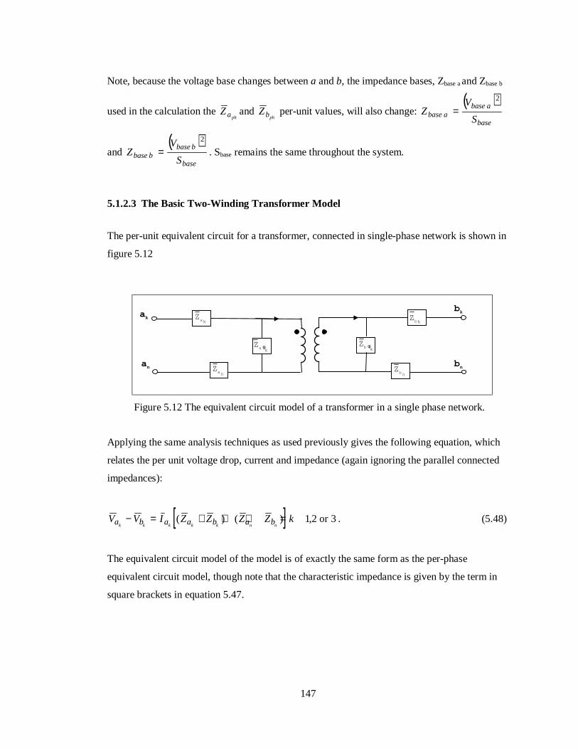
147
Note, because the voltage base changes between a and b, the impedance bases, Zbase a and Zbase b
used in the calculation the phaZ and
phbZ per-unit values, will also change: ( )
base
abaseabase S
VZ
2
=
and ( )
base
bbasebbase S
VZ
2
= . Sbase remains the same throughout the system.
5.1.2.3 The Basic Two-Winding Transformer Model
The per-unit equivalent circuit for a transformer, connected in single-phase network is shown in
figure 5.12
Figure 5.12 The equivalent circuit model of a transformer in a single phase network.
Applying the same analysis techniques as used previously gives the following equation, which
relates the per unit voltage drop, current and impedance (again ignoring the parallel connected
impedances):
[ ]V V I Z Z Z Z ka b a a b a bk k k k k n n− = + + + =( ) ( ) ,1 2 3or . (5.48)
The equivalent circuit model of the model is of exactly the same form as the per-phase
equivalent circuit model, though note that the characteristic impedance is given by the term in
square brackets in equation 5.47.
Zak
Zb kφZa φ
k
Zbk
ZanZbn
ak
an
bk
bn

148
The admittance that should be used in the calculation of the short-circuit driving port and
transfer admittance of the nodes to which the single phase transformer component connects is
)()(
1,
nnkk
kk
bababa ZZZZ
Y+++
= . (5.49)
Note that the models derived here, for the basic two-winding transformer and transformers in
three phase connections, are far from a complete catalogue of all possible transformer types:
transformers with off-nominal turns rations, 3 or more windings and transformers with different
permutations of three-phase connections are not considered. Weedy [2], Gross [3] and Stagg and
El-Abiad [5] give circuit models and derivations of characteristic equations for various other
transformer types.
5.2 Hybrid Components
The loads and sources which connect to the electrical network were described in the last chapter
as ‘hybrid’ components, as they also exist in other areas of the ESP-r model: the fabric, the plant
network, the flow network and the fluid volumes which from the interior space of the building.
As mentioned in the last chapter, the function of these hybrid components is to translate the
electrically related heat and fluid flow phenomena occurring in the building to the power flows,
which act as boundary data for the electrical network. These hybrid components are described in
the following sections.
5.2.1 Hybrid Load Components
5.2.1.1 Lighting and Small Power Loads
These power loads interact with both the thermal and electrical constituents of an ESP-r model,
in that they draw power from the electrical network and also dissipate heat into the thermal
zones. Currently, the thermal output from each power load manifests itself in the form of a
convective heat gain to the associated fluid volume, and as a radiative gain to the surface layers

149
of the multi-layered constructions surrounding the fluid volume. Recall, that the characteristic
equations which represent both the fluid volume and surface layers contained heat injection
terms that could represent the heat gain from internal sources (refer to equations 2.8 and 2.23
respectively). The total heat gain (W) from a power-consuming component i would be given by
q qi r
s
n
c s+
=∑
1
, (5.50)
where qicis the convective heat dissipated to the zone air volume and qr
s
n
s
=∑
1
is the sum of the
radiant heat dissipated to the surrounding surfaces.
In ESP-r, heat gains from equipment, lighting and occupants are defined as generic ‘casual
gains’[6]. Casual gains are time-variant and have radiant and convective portions. The temporal
variation of the gain during the simulation is obtained by multiplying a base gain (W) by a time-
varying profile, the magnitude of which varies between 0 and 1. Lighting gains can also be
subjected to daylight control. The thermal gains to the zone will therefore vary with time and
climate-dependent control action. To obtain the power consumption information from these
thermal gains it is necessary to hybridise them, i.e. relate their heat emission to their electrical
power consumption. The resulting hybrid casual gain and electrical entity is defined as a ‘zone
load’ component.
Each piece of power consuming equipment (in the form of a zone load) acts like a resistor,
dissipating heat to the environment with 100% efficiency. All real power consumed by the
component is assumed to be (eventually) dissipated as heat. The coupling between the heat
emission and the power consumption of the electrical load is given by the following trivial
equation.
q q Pi r
s
n
ic s+ =
=∑
1
. (5.51)

150
However, equation 5.51 provides only half of the information required for the translation of a
thermal gain to an electrical load, as the reactive power consumption is still unknown. Provision
of this information requires additional information from the modeller in the definition of the
zone load component. The basic information required by each casual gain is as follows.
Type Heat dissipated Radiant Fraction Convective Fraction Time on Time off
Equipment/ lighting/ occupant (W) % % (hrs) (hrs)
Table 5.1 Information provided for a casual gain.
This information was augmented with the electrical data given in the following table.
OperatingVoltage
Powerfactor (pf)
Load type Base powerconsumption
(=base heat load)
Connected phase Connected electricalnetwork node
(V) (0 - 1) capacitive,resistive, reactive
(W) (1,2,3 or all) (-)
Table 5.2 Additional information for a zone load.
The information allows all the relevant power flow information to be deduced from the thermal
heat dissipation of the casual gain. The reactive power consumption is given by
Q Ppf
i
i
= −
11
0 5.
0< pf ≤1 (5.52)
The power factor, pf, is defined as the ratio of the real power consumption of the component
divided by the magnitude of the apparent power consumption:
( )pf
P
P Qi
i
i i
=+2 2 0 5.
(5.53)

151
Note that the nature of the load determines the characteristics of its reactive power consumption.
If the load is inductive, then the reactive power consumption is assigned a positive value: +jQ .
If the load is capacitive, then the reactive power consumption is assigned a negative value: -jQ ;
reactive and capacitive power are diametrically opposed.
The real power consumptions of or many types of small power loads are given in [7], though this
reference contains no information on small load power factors. Information on lighting and
rotational load power consumptions and power factors is given in [8] and [9] respectively.
The other electrical information determines where the electrical load draws power from the
electrical network. In a balanced system, the load is assumed to draw power evenly from all
three phases of the power system. If the three-phase system is modelled comprehensively, the
connected node and phase data would be used to identify which node of a three-node array the
load would draw power from. Three-phase loads such as fans and pumps would power from all
three nodes. The voltage information can be used to check the operating voltage of the load
component against the predicted voltage of the connected electrical load; if the two differ
significantly, the zone load may be switched off by a control law (see section 5.5.1).
Note that the zone load component inherits all the characteristics of the associated casual gain,
and so the electrical load drawn from the network by each particular component will vary (as
was stated in section 5.2.1.1) both temporally and with climate influenced control.
As an example to illustrate the function of the zone load, consider the case of daylight
responsive luminaires. These will be controlled based on lighting levels inside a zone (calculated
by ESP-r or perhaps RADIANCE19 running in tandem with ESP-r), with the lighting control
altering the light output of the luminaires to maintain a constant illumination level. The control
of light output will affect the heat dissipated by the lights into to the zone and also their electrical
19 A lighting simulation tool produced by Lawrence Berkeley Laboratories

152
power consumption. The lighting hybrid component will therefore provide a time-varying power
flow boundary condition to the electrical network, while also providing a related time-varying
heat input to the lit zone. This hybrid component therefore acts as a coupling mechanism
between the thermal and electrical energy flows associated with the zone. The temporal variation
of these energy flows is primarily affected by the characteristics of the daylight control and the
prevailing climatic conditions. The concept of the hybrid component is shown schematically in
figure 5.
Figure 5.13 The schematic definition of a zone load.
5.2.2 Fans and Pumps
In ESP-r both fans and pumps can be labelled with the generic term ‘flow-inducing
components’, and exist in both the plant and fluid flow networks. Hence, in an integrated ESP-r
11:59:59
time dependencytime dependency
lightingcontrol
hybrid loads time-varyingpowerdemand
time-varyingheatdissipationandillumination
lighting sensors Climate (solar radiation)
electrical network

153
model, the flow inducing entities can be constructed using both a plant and fluid flow component
model; the fluid flow component calculates the pressure and flow characteristics, while the plant
component deals with the energy balance. The descriptions of both the plant and fluid flow
components for fans and pumps are given in [10] and [11].
To determine the power consumption of the fan or pump it is necessary to hybridise the plant
component model by the addition of an extra energy balance equation; this relates the
component flow characteristics to its power consumption. The foundation for this relation is an
equivalence of electrical and mechanical power, for which it is necessary to express the
mechanical power consumption, Pm (W), of the component in terms of the induced flow. This
relationship is given by the following equation.
Pm P
m
m
=& ∆η
(5.54)
&m is the induced mass flow rate (kg/s) resulting from the pressure rise, ∆P (Pa), across the
component and ηm is the mechanical efficiency of the flow-inducing component.
The following cubic polynomial relationship is given in [11] and relates the pressure rise and
flow rate in ESP-r’s flow inducing components (both pumps and fans).
∆P a am
am
am
o= +
+
+
1 2
2
3
3& & &
ρ ρ ρ(5.55)
ai=1 3.. are empirically obtained coefficients which fit equation 5.54 to the flow component’s
performance curve: this is usually supplied by the manufacturer; ρ is the working fluid density
(kg/m3).
The mechanical power required by the component is given by the substitution of equation 5.55
into equation 5.54:

154
Pm
a am
am
am
m
m
o= +
+
+
& & & &
η ρ ρ ρ1 2
2
3
3
. (5.56)
The mechanical power to the flow inducing component will be provided by an electrical motor,
the performance of which can be characterised by a conversion efficiency; this relates the
electrical power consumption of the motor to the mechanical power consumed inducing the flow
of working fluid. The relation is as follows.
P Pm e e= η . (5.57)
Substituting this expression into equation 5.56 gives the relationship between the induced flow
rate in the fan or pump and electrical power consumption of the electrical motor that would be
required to produce it.
Pm
a am
am
am
e
m e
o= +
+
+
& & & &
η η ρ ρ ρ1 2
2
3
3
. (5.58)
Note that as with the casual gain coupling equation (5.51), this equation only determines the real
power consumption of the fan or pump. To determine the reactive power consumption,
additional information must be used with the plant component. This additional information is
similar to that which augmented the casual gains.
Operating Voltage Power factor(pf)
Load type Efficiency of electricmotor
Connected phase Connectedelectrical node
(V) (0 - 1) capacitive,reactive
(0 - 1) (1,2,3 or all) (-)
Table 5.3 Additional information required for a power consuming plant component.
The reactive power consumption is calculated using equation 5.52, and assigned a positive or
negative value according to the load type.

155
Flow inducing components can be subject to control action, with the possibility of the flow rate
of each being varied according to temperature, pressure, humidity or some other sensed property
somewhere in the building model. Note also, that the thermophysical and fluid flow property
terms, used in the equation to calculate the power consumption, will vary as the pressure and
temperatures of the plant and flow networks change with time. As a consequence, the power
consumption of the plant component, like those of the casual gains, will also change with time
according to control action, thermal and flow conditions, providing a fluctuating power flow
boundary condition to the electrical network.
5.3 Hybrid Electrical Power Generation Component s
5.3.1 Small-Scale Combined Heat and Power (CHP)
A small scale combined heat and power system consists of two basic physical elements: an
engine and generator unit and a heat recovery system. The engine and generator provide power
to the electrical network, while the heat recovered (in the form of hot water) from the engine
jacket cooling water and exhaust gas can be used in the plant network.
Figure 5.14 A small-scale combined heat and power unit (from [12]).
engine unit
fuel supply(gas/diesel)
a.c. generator
engine jacketcooling waterheat exchanger
exhaust gas heatexchanger
cool waterreturn
hotwatersupply
poweroutput

156
Small scale combined heat and power systems, as shown in figure 5.14, are an integral part of a
building’s electrical and hot water services; the ESP-r model of the CHP unit was developed
with this in mind and can be integrated into both the plant and electrical network. The model is
constructed from a number of plant components. Each is modelled using control volumes:
• an engine and generator unit (a hybrid thermal electrical component);
• a cooling water heat exchanger (a purely thermal component);
• a gas - air heat exchanger (another purely thermal plant component).
The following sections describe these component models which, when combined with an ESP-r
plant network, form a model of a CHP system integrated into a building’s hot water services.
The plant network can, in turn, be integrated with the rest of the ESP-r building model, including
a coupling to the electrical network, forming a complete model of the CHP building-integrated
energy system. A system model of this type is shown in the exemplar of chapter 7.
5.3.1.1 The Engine and Generator Unit
The basis for the description of the engine and generator unit, as with all the other plant
components in ESP-r is the control volume. The Engine unit shown in figure 5.14 can be
represented by three control volumes:
• a combustion gas control volume;
• a solid engine block control volume;
• a coolant control volume.

157
The three-node model is a depiction of the basic thermodynamic processes occurring inside the
CHP unit. The combustion gas node represents the hot gas/fuel mixture contained in the engine
cylinders. This transfers heat to the engine block, which loses heat to the environment and
circulating cooling water, which is represented by the coolant control volume.
This three-node model is used as it can be easily integrated into an ESP-r model. The hot water
node can be coupled directly to ESP-r heating system components in a plant network (i.e. heat
exchangers, piping, pumps, etc.). The combustion chamber node can induce air from and exhaust
to a gas node representing atmospheric air. The connection of the model into an ESP-r plant
network is shown in chapter 7.
Figure 5.15 The three node model of the CHP engine unit.
The model is clearly an abstraction of the real engine and should be seen as a compromise
between a purely “black box” input/output model and more complex (though usually partial)
models such as that detailed by McCrorie et al. [13]. These are generally unsuitable for
integration into energy simulation tools as, for reasons of numerical stability, they require
processing with very small time steps (<.0000001s). The form of the model is shown in figure
5.15
fuel
combustionchamber node
coolantnode
solid engineblock node
i
i-1
j
kk-1
exhaust gascombustionair
w
qk,k-1
qi,j
qi,i-1
qj,k

158
5.3.1.1.1 The Combustion Gas Control Volume
The four-stroke cycle of the engine unit, consisting of an induction, compression, power and
exhaust stroke, can be considered as a continual, cycle-averaged thermodynamic process, if the
period of analysis is much greater than the time period of the individual strokes. This is
generally the case in an energy simulation. Further, if the cycle is averaged, then all the cylinders
can be lumped into the one control volume, because at any time t they will be at the same,
averaged state. Application of the first law of thermodynamics to the lumped control volume,
gives rise to the following one-dimensional, energy balance equation for the cycle-averaged
combustion process:
q q q wc i i i j i= + +−1, , . (5.59)
A barred variable represents a quantity averaged over all the phases of the four stroke-cycle.
qc is the heat release rate from fuel combustion (W), qi i−1, is the energy loss due to the intake
of cool combustion air into the cylinders (W), qi j, is the heat loss to the cylinder walls and wi is
the net mechanical work output from the combustion process (W).
The heat release from combustion can be calculated from
q m CVc c f= η & , (5.60)
where ηc is the efficiency of combustion in the engine cylinders, &m f is the fuel mass flow rate
(kg/s) and CV is its calorific value (J/kg).
The heat transfer due to the induction of air for the combustion process is given by
( )q m ci i i i i i, &− − − −= −1 1 1 1θ θ . (5.61)

159
&mi−1 is the mass flow rate of combustion air, and ci −1 is its specific heat (J/kgK). θi-1 is the
temperature of the gas leaving control volume i.
The heat transfer with the cylinder walls is calculated from the following equation.
q h Ai j cy cy j i, ( )= −θ θ (5.62)
θj is the temperature of the neighbouring engine block node hcy is the cycle-averaged heat
transfer coefficient (W/m2K) at the cylinder walls and Acy is the cycle averaged cylinder heat
transfer surface area (m2). hcy can be calculated by the time-averaged version of the empirical
equation given by Woschini [14]. Alternatively engine test data can be used to calculate the
overall cylinder wall conductance ( h Acy cy ) for the cycle-averaged combustion process; this is
discussed further in the next chapter.
Finally, the work output of the cylinder is the work of the engine unit after frictional losses have
been accounted for. Frictional losses are considered to be a heat gain in the cylinder and are
therefore lumped together with the heat release term qc .
Combining equations 5.59-5.62 gives the following fully explicit, characteristic equation for the
gas control volume at some time t (the effect of any thermal capacitance of the cylinder gases is
neglected).
− + + + =− − − − −( & ) &m c h A m c T h A T wit
i cyt
cy it
it
i it
cyt
cy jt t
1 1 1 1 1θ . (5.63)
The calculated temperature θi is the exhaust temperature of the combustion process, as all the
heat transfers, energy losses and transformations (i.e. heat to work) are accounted for in equation
5.63.

160
The work term w t is important as this is the link with the electrical output of the CHP unit and
enables the engine component to be made hybrid. The term represents the shaft power to the
rotor of the electrical generator, attached to the engine unit. The electrical power output of the
generator (W), which is fed into the electrical network, is calculated by
tee wP η= , (5.64)
where ηe is the electrical conversion efficiency of the generator attached to the CHP unit. The
reactive power output of the generator can be a controllable quantity20 and is discussed in section
5.3.2.1. Note it is also possible to explicitly model the generator attached to the CHP unit.
Generator equivalent circuits are given in appendix 2.
5.3.1.1.2 The Engine Block Control Volume
The basic form of the energy balance for the engine block node j is as follows
∞++= ,,, jkjijj
jj qqqt
cM∂
∂θ. (5.65)
The left hand side of equation 5.65 represents the thermal capacitance of the engine block; Mj is
its mass (kg), C j its volume-weighted, average specific heat (J/kgK). The terms on the right
hand side are the basic energy exchanges associated with the engine block.
q j,∞ is the heat loss from the engine block to the environment, which is given by
20 This is possible with synchronous generators, but not with asynchronous generators, which always
absorb reactive power (see appendix 2).

161
)(,, jjj Kq θθ −= ∞∞∞ , (5.66)
where Kj,∞ is the heat loss modulus from the engine exterior to the surroundings (W/K) and θ∞ is
the environmental temperature of the surroundings.
q j i, is the heat transfer from the walls of the cylinders, given by negative form of equation 5.62:
)(, jicycyij Ahq θθ −= . (5.67)
q j k, is the heat transferred to the cooling water flowing through the engine block, this is given
by:
)(,, jkckjkj Ahq θθ −= . (5.68)
Ac is the heat transfer surface area between the engine block and the cooling water, which has a
temperature θk. hj,k is the heat transfer coefficient between the cooling water and the engine
block. If the cooling water flows through the engine in enclosed channels, the following equation
(from [15]) can be used to determine the heat transfer coefficient, assuming fully turbulent flow
predominates:
nPrRe023.0Nu 8.0= . (5.69)
The dimensionless groupings of equation 5.69 are defined as follows.
The Reynolds number is given by Re = ρµ
VDh , where ρ is the coolant density (kg/m3), V is its
velocity (ms-1) and µ is the fluid viscosity (kg/ms). Dh is the hydraulic radius (m) of the enclosed
channel, given by Dh = ×4 flow area
wetted perimeter.

162
The Nusselt number is given by Nu =h D
kc h , where hc is the heat transfer coefficient between
the coolant and the channel wall and k is the conductivity of the coolant (W/mK).
The Prandtl number is given by Pr =c
kp µ
, cp is the specific heat of the coolant.
All the fluid parameters are evaluated at the mean temperature of the coolant and enclosed
channel walls, i.e. ( )θ θjt
kt+ / 2 .
As with the cylinder wall heat transfer equations, an alternative to the explicit calculation of the
coolant circuit heat transfer coefficient is to use test data to calculate the overall thermal
conductance ( h Aj k c, ) between the engine jacket and cooling water. This is discussed when
model calibration is considered in the next chapter.
Combining equations 5.65 to 5.68 and replacing the partial derivative with a backward
difference expression, gives the following explicit equation for the engine block temperature
θ jt t+ ∆ .
)()()( ,tj
te
ttj
tkc
tkj
tj
ticy
tcy
tj
ttjt
jtj AhAhAh
tcM θθθθθθ
θθ−+−+−=
∆−
∞∞
∆+
(5.70)
Combining this explicit expression with its implicit counterpart creates the following familiar
form of characteristic equation for the engine block control volume:

163
.2
2
,,
,
,
te
ttkc
tkj
ticy
tcy
tjc
tkjcy
tcy
tj
tj
tte
ttttkc
ttkj
tticy
ttcy
ttjc
ttkjcy
ttcy
ttj
ttj
AhAhAhAhAht
cM
AhAhAh
AhAht
cM
∞∞
∆+∞
∆+∞
∆+∆+∆+∆+
∆+∆+∆+∆+∆+
+++
++
∆=
−−−
++
∆
θθθθ
θθθ
θ
(5.71)
5.3.1.1.3 The Cooling Water Control Volume
The basic energy balance equation for the cooling water control volume is
jkkkk
kk qqt
cM ,1, += −∂∂θ
. (5.72)
The left-hand side of the equation represents the thermal capacity of the cooling fluid
encapsulated by the control volume (i.e. contained in the enclosed channels of the engine block);
Mk is its mass and Ck is its specific heat. The qk, k-1 term is the heat exchange caused by coolant
entering the control volume from a connected node (k-1) in the plant network:
q m c T Tk k k k k k, & ( )− − − −= −1 1 1 1 . (5.73)
The qk,j term is the negative of the heat exchange with the engine block, which was defined in
equation 5.68.
Following the same process as was used with the engine block node, the following characteristic
equation emerges for the cooling water control volume:

164
.2
2
,11,1
,11
,1
11
1
1
tjc
tjk
tk
tp
tk
tkc
tjk
tp
tk
tp
tk
ttjc
ttjk
ttk
ttp
ttk
ttkc
ttjk
ttp
ttk
ttp
ttk
AhcmAhcmt
cM
Ahcm
Ahcmt
cM
kk
k
k
k
k
θθθ
θθ
θ
++
++
∆=
−−
++
∆
−−−
∆+∆+∆+−
∆+∆+−
∆+∆+∆+∆+−
∆+∆+
−−
−
−
&&
&
&
(5.74)
5.3.1.2 The Cooling Water Heat Exchanger
This component is constructed from two, mixed-property control volumes, which represent the
hot and cold side of the heat exchanger, as shown in figure 5.16. The properties of the solid
casing of the heat exchanger are assumed to be evenly distributed between these two nodes.
5.3.1.2.1 The Hot-Side Control Volume
Figure 5.16 The control volume representation of the heat exchanger.
c
h-1h
c-1
hot-side node
cold-side nodeqh,c

165
Applying the same process as was used in the derivation of the engine unit’s characteristic
equations gives the following expression for the hot side of the heat exchanger.
.2
2
,11111
,11111
tch
th
th
th
th
th
th
th
th
ttch
tth
tth
tth
tth
tth
tth
tth
tth
cmcmt
cM
cmcmt
cM
φθθ
φθθ
++
+
∆=
−−
+
∆
−−−−−
∆+∆+−
∆+−
∆+−
∆+∆+−
∆+−
∆+∆+
&&
&&
(5.75)
Mh is the mass of the casing and encapsulated fluid on the hot side of the heat exchanger and
ch is their volume weighted, average specific heat. &mh −1 is the mass flow rate of hot fluid
(engine cooling water) into the heat exchanger with a specific heat ch −1 . The heat flux between
the hot and cold side of the heat exchanger φh c, , at some time t, is calculated from
[ ]φ η θ θh ct
eff ht
ctC, min ( )= −− −1 1 . (5.76)
The bracketed term represents the maximum possible heat exchange between the hot and cold
side of the heat exchanger. The two temperatures are the inlet temperatures to the hot and cold
side of the heat exchanger respectively. The Cmint term is the minimum &m cc
tpt
cor &m ch
tpt
h. ηeff is
the effectiveness of the heat exchanger, which varies according to the type of heat exchanger.
The well-known number of transfer units (NTU) method [16] is used to calculate this term. As
an example, consider a plate heat exchanger in counter flow; the equation for ηeff is
ηβ
β
βeff
NTU
NTU
e
e=
+−
− −
− −1
1
(1 )
(1 ) (5.77)

166
where β is the ratio Cmint/Cmax
t, The Cmaxt term is the maximum of &m cc
tpt
cor &m ch
tpt
h. Effectiveness
equations for different configurations of heat exchanger are given by Kays et al. [16]. The NTU
term is given by
NTUK
C
t
t=min
, (5.78)
K is the overall heat transfer modulus (W/K) between the hot and cold side of the heat
exchanger: this is defined later.
5.3.1.2.2 The Cold-Side Control Volume
An almost identical control volume characteristic equation to that of the hot-side can be derived
for the cold-side of the heat exchanger:
.2
2
,111
,111
1
1
thc
tc
tc
tc
tc
tp
tc
tc
th
tthc
ttc
ttc
ttc
ttc
ttp
ttc
ttc
ttc
cmcmt
cM
cmcmt
cM
c
c
φθθ
φθθ
++
+
∆=
−−
+
∆
−−−
∆+∆+−
∆+∆+−
∆+∆+∆+−
∆+∆+
−
−
&&
&&
(5.79)
The terms of equation 5.79 have the same meaning as those of equation 5.75, the subscript c
refers to the cold side of the heat exchanger. φc,h is the negative of the flux exchange expression
in the hot side characteristic equation.
The calculation of the effectiveness, which in turn is used to calculate the flux exchange between
the hot and cold sides of the heat exchanger, requires the calculation of the heat exchange
modulus K. This can be expressed as
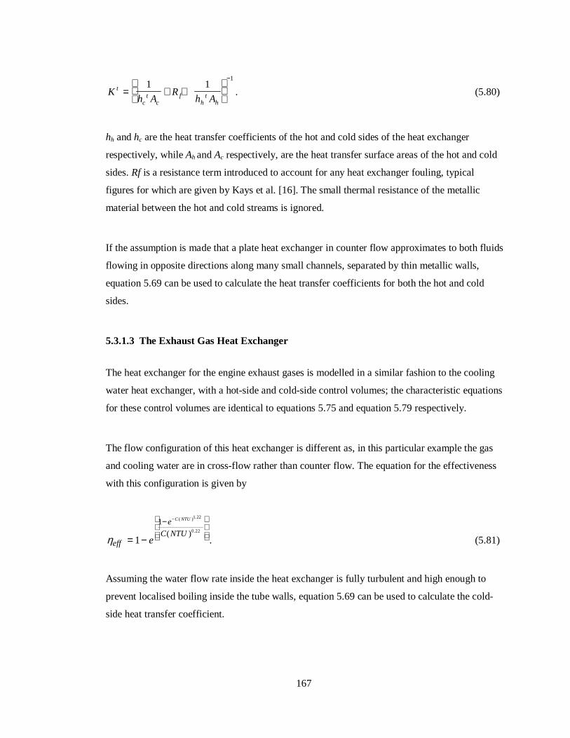
167
Kh A
Rh A
t
ct
cf
ht
h
= + +
−1 1
1
. (5.80)
hh and hc are the heat transfer coefficients of the hot and cold sides of the heat exchanger
respectively, while Ah and Ac respectively, are the heat transfer surface areas of the hot and cold
sides. Rf is a resistance term introduced to account for any heat exchanger fouling, typical
figures for which are given by Kays et al. [16]. The small thermal resistance of the metallic
material between the hot and cold streams is ignored.
If the assumption is made that a plate heat exchanger in counter flow approximates to both fluids
flowing in opposite directions along many small channels, separated by thin metallic walls,
equation 5.69 can be used to calculate the heat transfer coefficients for both the hot and cold
sides.
5.3.1.3 The Exhaust Gas Heat Exchanger
The heat exchanger for the engine exhaust gases is modelled in a similar fashion to the cooling
water heat exchanger, with a hot-side and cold-side control volumes; the characteristic equations
for these control volumes are identical to equations 5.75 and equation 5.79 respectively.
The flow configuration of this heat exchanger is different as, in this particular example the gas
and cooling water are in cross-flow rather than counter flow. The equation for the effectiveness
with this configuration is given by
ηeff
e
C NTUe
C NTU
= −
−
−
1
11 22
0 22
( ) .
.( ). (5.81)
Assuming the water flow rate inside the heat exchanger is fully turbulent and high enough to
prevent localised boiling inside the tube walls, equation 5.69 can be used to calculate the cold-
side heat transfer coefficient.

168
The following equation (given in [17]) can be used to calculate the heat exchange coefficient
from the combustion gas as it flows over the tubes containing the cooling water:
Nu = 0 33 0 6 0 3. Re Pr. .λ . (5.82)
λ is an empirical constant, dependent upon the tube bundle geometry. Note that the
thermophysical properties of the hot combustion gas are slightly different from those of air;
combustion gas property tables [18] can be used to determine them. However, for the
stochiometric combustion of natural gas (used in most CHP units), 96% of the combustion gas is
air [19] hence the use of the thermophysical properties of air should not lead to a large
discrepancy. Note that the mean temperature of the tube wall (assumed to be close to the cooling
water temperature) and adjacent combustion gas is used in the calculation of equation 5.82.
5.3.1.3.1 The Complete CHP Unit
The components of the CHP unit connect together as in figure 5.17.
Figure 5.17 The complete CHP unit model.
m
l
i
j
o
n
hot water to othercomponents in theplant network
return fromconnectedcomponents
k
exhaustoutletcombustion
air
enginecoolingwater
exhaust gas

169
CHP is discussed further in the technology review of appendix 2.
5.3.2 Photovoltaics
To enable the modelling of photovoltaic (PV) components in ESP-r, the concept of the ‘special
material’ was introduced [20]21. This allows PV elements of the building facade to be treated in
the same way as all other solid elements of the building fabric, while accounting for the special
power producing nature of these materials.
Building-integrated PV components are constructed of several elements: the PV material,
conductors, a binder and a casing. The PV material is the power producing element, the
conductors carry away the material’s power output, while the casing encloses the PV material
and the conducting elements, providing both protection and rigidity. The binding material glues
the whole construction together. At a fundamental level, the facade-integrated PV component
can be represented as an ESP-r multi-layered construction (see section 2.2.4): the PV material
forming one layer of this construction. It is the PV layer that is designated as a ‘special material’.
Consider the case of a photovoltaic facade element as shown in figure 5.18. This element, a PV
panel, consists of four layers of material: inner and outer glazing, a PV material layer and a resin
binder. Note that the PV layer in the panel consists of a number of solar cells, which incorporate
both the PV material and conducting elements. The individual solar cells, connected together,
are considered to be a layer of homogeneous PV material. Solar cells are described in more
detail in appendix 1.
21 Note that the special material concept is not only used in the modelling of photovoltaic materials, it has
also been applied in the modelling of special glazing elements [18].

170
Figure 5.18 A Multi-layered construction incorporating a photovoltaic material.
Focusing on the layer of PV material, this is an internal element of the construction (see section
2.2.4), which can be represented by 3 control volumes: a homogeneous layer and two mixed-
property layers (see figure 5.18).
Figure 5.19 PV material control volumes
outer glazing layer
Inner glazing layer
PV layerresinbinder
incidentsolarradiation
mixed-propertyPV node
homogeneous PVnode
Outer glazinglayer
resin
mixed-propertyPV layer
not to scale
incident solarradiation
i+1…ii-1

171
Recall from chapter 2 that the characteristic equations for these control volumes were as follows.
For the internal homogeneous element (node i):
( )2
2
1 12
12 1
12 1
1 12
12 1
12
ρθ θ θ
ρθ θ θ
i i i i i i
iit t i i
iit t i i
iit t i e
t t
i
i i i i i i
iit i i
iit i i
i
c
t
k k
x
k
x
k
x
q
x y z
c
t
k k
x
k
x
k
x
∆ ∆ ∆ ∆ ∆ ∆ ∆
∆ ∆ ∆ ∆
∆ ∆ ∆∆
++
− − −
= ++
+ +
+ − + +++ −
−+
+
+ − ++
−
, , , ,
, , , ,
( )it i e
t
i
q
x y z− +1 ∆ ∆ ∆
.
The thermophysical properties of this control volume would be those of the PV material.
For the mixed-property layers, the characteristic equation of (node i-1) is given by
2 2 2
2
1 1 1 1
1 1 2 1
2 1 1
1 1 2 11
1 1
1 1 2 1
ρθi i i i i
i i i i i
i i i
i i i i iit t
i i i
i i i i i
c
t
k R x
x x x R
k R x
x x x R
k R x
x x x R
− − − −
− − − −
− − −
− − − −−+
− −
− − − −
+++
+++
−
++
∆∆
∆ ∆ ∆∆
∆ ∆ ∆
∆∆ ∆ ∆
∆,
, ,
,
, ,
,
, ,
( ) ( )
( ) ( )
−
++
−
= +++
++
+ − − −
− − − −−+ −
+
−
− − − −
− − − −
− −
θ θ
ρ
it t i i i
i i i i iit t i
t te
i
i i i i i
i i i i i
i i
k R x
x x x R
q
x y z
c
t
k R x
x x x R
k R x
∆ ∆∆∆
∆ ∆ ∆ ∆ ∆ ∆
∆∆
∆ ∆ ∆∆
2 1 1
1 1 2 12
1
1
1 1 1 1
1 1 2 1
2 1
2
2 2 2
,
, ,
,
, ,
,
( )
( )i
i i i i iit
i i i
i i i i iit i i i
i i i i iit i
t
x x x R
k R x
x x x R
k R x
x x x R
q
−
− − − −−
− −
− − − −
− − −
− − − −−
−
+
+
++
+
++
+
1
1 1 2 11
1 1
1 1 2 1
2 1 1
1 1 2 12
12 2
∆ ∆ ∆
∆∆ ∆ ∆
∆∆ ∆ ∆
( )
( ) ( )
, ,
,
, ,
,
, ,
θ
θ θ ( )e
ix y z∆ ∆ ∆ −1
.
For node i+1:

172
2 2 2
2
1 1 1 1
1 1 2 1
2 1 1
1 1 2 11
1 1
1 1 2 1
ρθi i i i i
i i i i i
i i i
i i i i iit t
i i i
i i i i i
c
t
k R x
x x x R
k R x
x x x R
k R x
x x x R
+ + + +
+ + + +
+ + +
+ + + +++
+ +
+ + + +
+++
+++
−
++
∆∆
∆ ∆ ∆∆
∆ ∆ ∆
∆∆ ∆ ∆
∆,
, ,
,
, ,
,
, ,
( ) ( )
( ) ( )
−
++
−
= +++
++
+ + + +
+ + + +++ +
+
+
+ + + +
+ + + +
+ +
θ θ
ρ
it t i i i
i i i i iit t
it t
i
i i i i i
i i i i i
i i
k R x
x x x R
q
x y z
c
t
k R x
x x x R
k R x
e∆ ∆∆
∆∆ ∆ ∆ ∆ ∆ ∆
∆∆
∆ ∆ ∆∆
2 1 1
1 1 2 12
1
1
1 1 1 1
1 1 2 1
2 1
2
2 2 2
,
, ,
,
, ,
,
( )
( )i
i i i i iit
i i i
i i i i iit i i i
i i i i iit
it
x x x R
k R x
x x x R
k R x
x x x R
q
+
+ + + ++
+ +
+ + + +
+ + +
+ + + ++
+
+
+
++
+
++
+
1
1 1 2 11
1 1
1 1 2 1
2 1 1
1 1 2 12
12 2
∆ ∆ ∆
∆∆ ∆ ∆
∆∆ ∆ ∆
( )
( ) ( )
, ,
,
, ,
,
, ,
θ
θ θ ( )e
x y zi
∆ ∆ ∆ +1
.
The thermophysical properties of the two mixed-property volumes would be the mass weighted
averages of the PV material and resin binder (node i-1), or the PV material and the outer glass
cover sheet (node i+1).
In the construction of figure 5.18, solar radiation is transmitted to the surface of the PV layer
through the glass cover material. The calculation of the intensity of solar radiation incident on
the glass surface is handled by ESP-r’s solar processing algorithms. The incident radiation is a
function of the surface geometry, site location (latitude and longitude), shading and the temporal
characteristics of the climatic data at the simulation time step. Refer to Clarke [10] for more
details.
In most other construction materials (excluding phase change materials), the absorption of solar
radiation would result in a temperature rise, through the conversion of the absorbed solar
radiation to heat. The absorption of this radiation at the surface of the PV material, node i+1, is
represented by the qi+1 heat injection term in its characteristic equation. However, a PV material
is regarded as a ‘special material’ in ESP-r, as not all the absorbed solar is converted to heat: a
proportion is converted to electrical energy, and transported away as electrical current in the
conducting elements. The characteristic equation of the PV material control volumes must

173
therefore be altered to take account of this fact, by the addition of an extra term to account for
the production of electrical energy (e.g. for node i+1).
2 2 2
2
1 1 1 1
1 1 2 1
2 1 1
1 1 2 1
1
1 1
1 1 2 1
ρθi pi i i i
i i i i i
i i i
i i i i i
it t
i i i
i i i i i
c
t
k R x
x x x R
k R x
x x x R
k R x
x x x R
+ + + +
+ + + +
+ + +
+ + + +++
+ +
+ + + +
+++
+++
−
++
∆∆
∆ ∆ ∆∆
∆ ∆ ∆
∆∆ ∆ ∆
∆,
, ,
,
, ,
,
, ,
( ) ( )
( ) ( ) −++
−
−
= +++
+
+ + + +
+ + + +++ +
+++
+
+ + + +
+ + + +
+ +
θ θ
ρ
it t i i i
i i i i i
it t i
t tit t
i
i pi i i i
i i i i i
i i
k R x
x x x R
q q
x y z
c
t
k R x
x x x R
k
e p∆ ∆∆ ∆∆
∆ ∆ ∆ ∆ ∆ ∆
∆∆
∆ ∆ ∆
2 1 1
1 1 2 1
2
1 1
1
1 1 1 1
1 1 2 1
2
2
2 2
,
, ,
,
, ,
,
( )
( )1 1
1 1 2 1
1
1 1
1 1 2 1
2 1 1
1 1 2 1
2
1
2
2 2
R x
x x x R
k R x
x x x R
k R x
x x x R
q
i
i i i i i
it
i i i
i i i i i
it i i i
i i i i i
it i
t
++
+
++
+
++
+
+
+ + + ++
+ +
+ + + +
+ + +
+ + + ++
+
∆∆ ∆ ∆
∆∆ ∆ ∆
∆∆ ∆ ∆
( )
( ) ( )
, ,
,
, ,
,
, ,
θ
θ θ ( )e p
q
x y z
it
i
− +
+
1
1∆ ∆ ∆
The q
x y zit
p
i
+1
( )∆ ∆ ∆term represents the electrical power (W) produced by the PV layer per unit
volume at some time t. Note that the term is of the opposite sign to the heat injection term.
Hence, when producing electrical power, the temperature of the PV layer would be cooler than
would occur in the situation where no power was produced.
Note that the PV component can either be transparent or opaque22. Radiation will be absorbed in
all three nodes of the transparent material. It is assumed that all power production in a
transparent PV material occurs at the centre node of the layer (node i). The heat injection term
would be altered in the same manner as that of node i+1. In an opaque PV material all the solar
energy is absorbed in the first (mixed) layer of material. Again power production is assumed to
occur at the homogeneous node in the PV material. Note that the PV layer is thin compared to
22 The fundamentals of PV materials are discussed in appendix 1.

174
the other layers in the construction and so the relative positions of solar absorption and power
production within the layer are thermodynamically unimportant.
The previous paragraphs have shown how a PV panel can be modelled thermophysically in ESP-
r by its definition as a multi-layered construction. This allows the temperature, and more
importantly the intensity of solar radiation absorbed in the solar cell to be calculated. As will be
shown below, these quantities are required in the calculation of the power generated by the PV
element, which in turn is a quantity required by the characteristic equations of the PV material
control volumes. The temperature, solar incident radiation and PV power output are therefore
coupling variables between the thermal and electrical equations of the PV material.
To calculate the power produced by the PV material, its central, homogeneous thermal control
volume must be augmented with electrical control volumes; one for each solar cell in the layer.
The PV material therefore becomes a hybrid thermal/electrical component. Each electrical
control volume consists of an equivalent circuit model, which encapsulates the electrical
characteristics of the solar cell. This is shown in figure 5.20.
Figure 5.20 The equivalent circuit of the solar cell.
The circuit model shown above is based on that described by Buresch [21] and many others. The
current source represents the current generated by absorption of solar radiation in the cell: the
IL I
d
Ii
ilightgeneratedcurrent
diodecurrent
output current
Vi output voltage
+
-
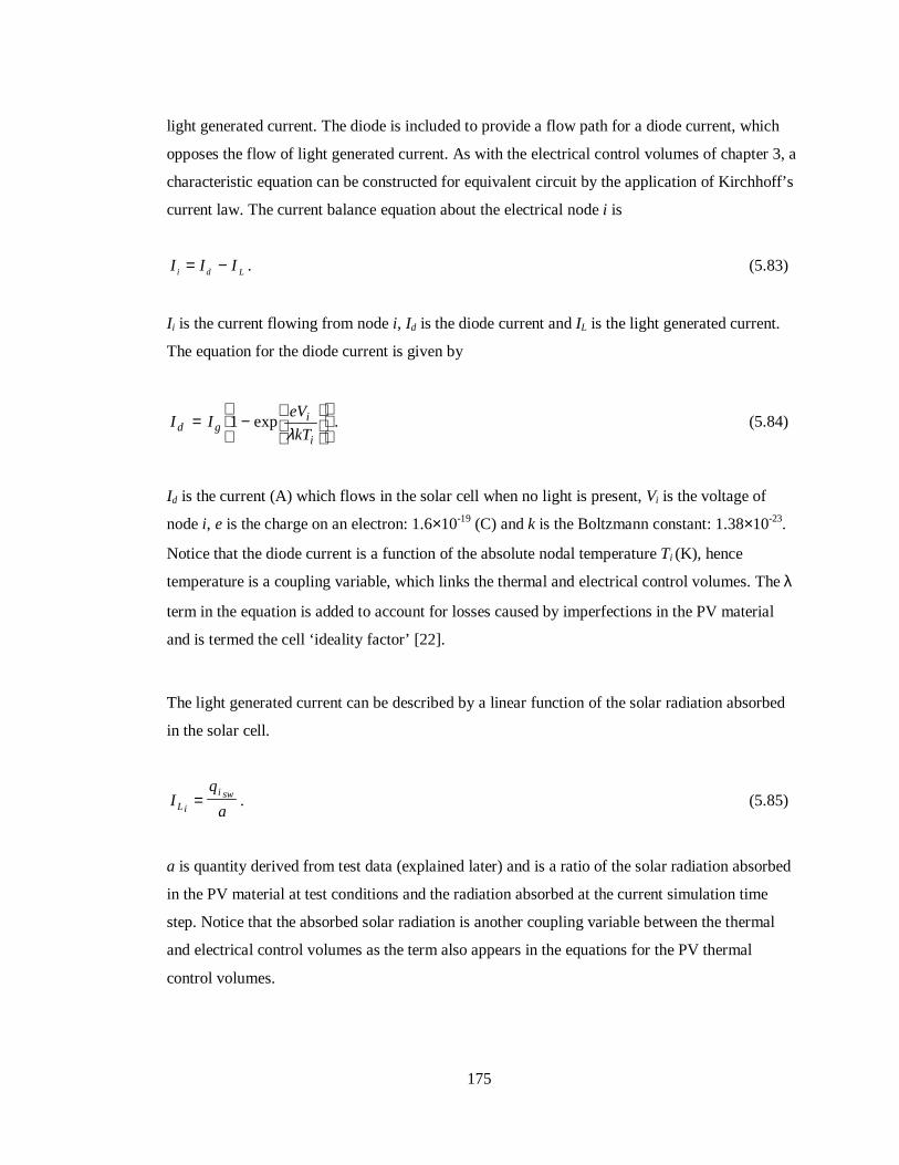
175
light generated current. The diode is included to provide a flow path for a diode current, which
opposes the flow of light generated current. As with the electrical control volumes of chapter 3, a
characteristic equation can be constructed for equivalent circuit by the application of Kirchhoff’s
current law. The current balance equation about the electrical node i is
I I Ii d L= − . (5.83)
Ii is the current flowing from node i, Id is the diode current and IL is the light generated current.
The equation for the diode current is given by
I IeV
kTd gi
i
= −
1 exp
λ. (5.84)
Id is the current (A) which flows in the solar cell when no light is present, Vi is the voltage of
node i, e is the charge on an electron: 1.6×10⁻¹⁹ (C) and k is the Boltzmann constant: 1.38×10⁻²³.
Notice that the diode current is a function of the absolute nodal temperature Ti (K), hence
temperature is a coupling variable, which links the thermal and electrical control volumes. The λ
term in the equation is added to account for losses caused by imperfections in the PV material
and is termed the cell ‘ideality factor’ [22].
The light generated current can be described by a linear function of the solar radiation absorbed
in the solar cell.
Iq
aLi
i sw= . (5.85)
a is quantity derived from test data (explained later) and is a ratio of the solar radiation absorbed
in the PV material at test conditions and the radiation absorbed at the current simulation time
step. Notice that the absorbed solar radiation is another coupling variable between the thermal
and electrical control volumes as the term also appears in the equations for the PV thermal
control volumes.

176
Substituting the equations for Id and IL into the current balance equation gives
I IeV
kT
q
ai gi
i
i sw= −
−1 exp λ . (5.86)
The d.c. power output from the solar cell (W) is given by
P V I V IeV
kT
V q
ai i i i gi i i sw= = −
−1 exp
λ. (5.87)
The output for the entire PV layer in the multi-layered construction is calculated by multiplying
the individual cell output by the number of cells in the layer:
P n V IeV
kT
V q
alayer i gi i i sw= × −
−
1 expλ
. (5.88)
Notice that the equation for the power output from the PV layer contains numerous unknowns:
Vi, a, λ and Ig , hence the solution of this equation requires that these unknowns are defined.
The unknown terms can be calculated if test data is available for the PV panel component: the
open circuit voltage Vocp, the short circuit current Iscp, the optimum operating voltage Vmpp and the
optimum operating current Impp. All the properties are measured at a reference temperature of Tref
(K) and absorbed solar radiation flux23, qi sw ref
⊥ (W).
23 Note that in most cases the given test value for PV components is the radiation incident on the outer
cover of the panel at an incidence angle of 0o. For equation 5.81 the radiation absorbed by the PV material
at these reference conditions is required. This can be calculated from test value of incident solar radiation
if the angular dependent optical properties of the PV material and glass cover sheet are known.

177
Note that the previously defined equations were derived in terms of cell characteristics and not
panel characteristics. The test data must therefore be converted to cell values. This is a
straightforward process: for a panel with x branches of cells connected in parallel, and y cells
connected in series in each branch (the total number of cells is n x y= × ). The values to use in
the cell equations are as follows.
x
II psc
sc = , x
II pmp
mp = and VV
yococp= ,V
V
ymp
mp p= .
The extra p subscript denotes a quantity relating to the entire panel.
The test data can then be used as boundary condition information for the derived equations,
enabling the calculation of the unknown terms as follows.
For the equivalent circuit of the PV material (figure 5.20), in the open circuit conditions, Vi = Voc
and Ii = 0. Substituting these values into equation 5.86 gives
I IeV
kTL g
oc
ref
=
exp
λat qi sw ref
⊥ . (5.89)
In the short circuit condition Ii = Isc, Vi = 0 and Id = 0, therefore
I IL sc= − at q Ti sw refref
⊥ , . (5.90)
Combining these two equations and re-arranging gives an expression for the unknown current,
Ig, in terms of measured test quantities Voc, Isc and Tref :

178
II
eV
kT
gsc
oc
ref
= −
−
exp
λ1
. (5.91)
Ig also varies with the temperature of the PV material (i.e. the temperature of the nodes in the PV
material). The following equation (given in [23]) describes the change in Ig with temperature, in
relation to the reference temperature Tref.
[ ]I Ig T
T T
g Ti
i ref
ref( )
( )
( )=−
2 σ . (5.92)
Substituting into equation 5.91 gives
II
eV
kT
g
T T
sc
oc
i ref
= −
−
−
2
1
σ
λexp
. (5.93)
Note that the variable σ is an empirical constant, whose value varies with the characteristics of
the PV material. Buresch uses a value of σ = 10, while a value of σ = 15 was found by
experimentation in [24]. The derivation of this value is discussed in the next chapter.
The ideality factor λ is calculated from the following equation
( )λ =
−
−
e
kTV V
I I
I
ref
mp oc
sc mp
sc
ln
. (5.94)
Finally, the variable a is calculated from

179
ai swref
i
=⊥αα , (5.95)
where αi is the absorbed solar radiation (W/m3) in the photovoltaic material layer at the current
simulation time step (already calculated by ESP-r).α i swref⊥ is the solar radiation absorbed at test
conditions (W/m3).
The power output for the panel (equation 5.88) can now be solved if Vi is known. Very often the
power output from a PV component is controlled such that it always operates at the optimum
power producing conditions: the ‘maximum power point’ (see appendix 1). At this condition
0=i
i
V
P
∂∂
. Taking the derivative of equation 5.88 with respect to Vi gives the following
transcendental equation for the voltage Vi at the maximum power point:
1 1+ =
+
I
I
eV
kT
eV
kTL
g
i
i
i
i
expλ λ
. (5.96)
The iterative solution of this equation for Vi and its substitution into equation 5.88 allows the
power output from the PV element to be calculated. This can then be inserted into the control
volume characteristic equations (described previously) for the calculation of the PV element
temperature. In crystalline PV materials, the thermal and electrical equations are closely
coupled: the electrical output of the PV panel is a function of the PV layer temperature, which is
affected by the power output of the PV material. Note that the power output of the PV element is
d.c. and so before it can be injected into an a.c. electrical network it must undergo an inversion
process; this is discussed, along with an examination of solar cell physics, in appendix 1.

180
5.4 Control in Integrated Simulations
So far this chapter has described the components necessary for the modelling and simulation of
electrical and building-integrated energy systems. However, one other vital constituent of the
simulation model has yet to be discussed: control.
Control plays an important part in both the simulation of the electrical network and in the
simulation of the overall integrated model. The basis of control in ESP-r, the control loop [10],
was described in chapter 2. The control loop imposes a user-defined control action on individual
zones, plant or flow components. The operation of each control loop is dictated by a control law.
An additional layer of control, ‘global control’ (MacQueen [25]), has been added to ESP-r,
which is active at the highest level within the integrated simulation. Global control supervises
the activity of the lower level control loops, based on a high-level global control strategy.
The two levels of control form a control hierarchy and enable ESP-r to simulate many types of
building control including building energy management systems [25]. Both of these levels of
control affect the simulation of electrical power flow, as will be described in the following
sections.
5.4.1 The Action of the Control Loop on the Electrical Network
Control loops play an important part in the electrical simulation, as they regulate the power
demand of many of the hybrid components attached to the electrical network. Fans, pumps and
lighting can all be affected by control action. As mentioned in chapter 2, a control action
operates to bring about a user defined control objective. This is achieved by altering the state of
a controlled entity (e.g. a plant component) based on the interaction of a sensed property (time,
temperature, pressure, wind speed, daylight, etc.) and a control law. When control is used in the
regulation of the hybrid components, which supply the power flow boundary conditions to the
electrical network, it implicitly couples these boundary conditions to sensed environmental
conditions in all other constituent parts of the building model, e.g. temperatures in the zones,
plant component states, flow rates, etc.

181
5.4.2 The Addition of an Electrical Control Loop
The concept of the control loop has been extended to operate within the electrical network itself,
in the form of an electrical control loop, the principles of which are exactly the same as all other
control loops in ESP-r. The electrical control loop senses a state variable at a point in the
electrical network (voltage, current, real or reactive power). Based on the state of the sensed
variable, an electrical control law acts to bring about a user-defined control objective, through
the actuation of another electrical state variable at another point in the network. Note that the
explicit modelling of the electrical network is particularly important in this case as it is the
means by which the voltage variables necessary for the input to the control algorithm can be
calculated.
5.4.3 A Generator Voltage Control Law
As an example of electrical control, recall that the reactive power output from the CHP unit,
fitted with a synchronous generator, was a controllable quantity; this controllability is used for
voltage regulation in power systems and a controller of this type has been installed in ESP-r. The
basis of the voltage regulation is to maintain a user-defined constant voltage at the generator
terminals (the node in the electrical network to which the generator is attached) by varying its
reactive power output to exactly meet the demands of the coupled electrical system. However,
there are limits to the reactive power output of the generator; once these limits are reached, the
voltage across the generator terminals can no longer be fixed and will float. The form of the
control law is shown in figure 5.21.

182
Figure 5.21 Synchronous generator voltage control.
5.4.4 Global Control
The use of control to iteratively couple the electrical network solver into the overall solution
process was discussed in section 4.4. One control scenario discussed was where the electrical
network could only supply a finite amount of energy to the building: either because of tariff
limitations or because of a finite generating capacity, e.g. where the building operates a stand-
alone electrical energy generation system. When the limits of electrical power supply are
reached, the global controller would act to reduce the demand of the building by shutting off
power consuming components thereby explicitly affecting the building environmental conditions
based on set electrical energy limits. This requires the re-calculation of the building, plant and
flow network environmental states based on the new power supply conditions.
The foundations to achieve this coupling between the electrical network and the building
environmental conditions already exist, in the form of high-level level global control. One such
controller, the ‘global capacity controller’ [25], is ideally suited to the task of electrical energy
management.
P
a.c. generator
electrical network
variable Q:f(excitation)
voltagecontrol
actuation:generatorexcitation level(see appendix 2)
Vi
coupledelectrical node
sensed variable -the voltage at thegenerator terminals
fixed voltage set-point

183
At each simulation time step, the global capacity controller supervises the state of the plant and
control loops based on user defined capacity limits; these limits can be thermophysical such as
heat output or fluid flow. The controller monitors the level of the thermophysical property and, if
the capacity limit is exceeded, acts to sequentially close down selected components (e.g. lights
or items of plant) to bring the level of the relevant property back within set limits.
In an electrical context, capacity limiting would work as follows. The system power
consumption would be determined from the power imported via the reference node of the
electrical network. If the user defined power consumption capacity limit is exceeded, the global
control would act to sequentially zero the output of selected control loops, shutting down the
component to which they are connected, until the monitored power consumption falls back
below the capacity limit. The overall solution for the building, at the affected time step, would
then be re-calculated based on the new control state. This global control action is represented
schematically in figure 5.22
It should be noted that the addition of the electrical network and power producing components
opens up a range of possibilities for the development of new ESP-r control strategies, using the
range of controllable quantities (electrical power flows and state variables) calculated in the
electrical network. This short section has only discussed a very few of these new control
possibilities, more are discussed in chapter 8.

184
Figure 5.22 The global capacity controller, applied in an electrical context.
5.5 Summary
This chapter has described the various component types that have been added to ESP-r for use in
the integrated simulation of the electrical network and building-integrated energy systems:
• the electrical conductors and transformers which couple the control volumes in the electrical
network;
P Q,∑
capacitycontroller
powerconsumption
capacity limit
on/off
controlloop 1
controlloop 2
controlloop 3
controlloop 4
controlloop 5
controlloop 6
on/off on/off on/off on/off on/off
P,Q P,Q P,Q P,Q P,QP,Q
electrical network

185
• the hybrid load and plant components which draw power from the electrical network, while
simultaneously affecting thermophysical conditions in other parts of the building network;
• the hybrid and plant components can be used in the modelling of building-integrated energy
systems.
The use of these component models within the context of an integrated simulation is
demonstrated in chapter 7. However before this is done the next chapter describes the techniques
used to validate both the developed models and the electrical network solver described in chapter
3.

186
5.6 References
1. Oateley C, Electric and magnetic fields - an introduction, Cambridge University Press,
1980.
2. Weedy B M, Electric Power Systems, Wiley, New York, 1979
3. Gross C A, Power System Analysis, Wiley, New York, 1986.
4. BICC, Electric Cables Handbook, Blackwell, 1990.
5. Stagg G W and El-Abiad, Computer Methods in Power System Analysis, McGraw-Hill, New
York, 1968.
6. ESP-r user’s guide, Energy Simulation Research Unit, Glasgow, 1998.
7. Parsloe C and Hejab M, Small power loads, Building Services Research and Information
Association Technical Note TN8/92.
8. Chapman D F, Slater A I, Isaacs A L, Energy limiters - their place in lighting control, BRE
Report 114/3/4, 1986.
9. Capehart B L, Slack K D, Power factor benefits of high efficiency motors, Energy
Engineering, Vol. 93, No. 3, 1996.
10. Clarke J A, Energy simulation in building design, Adam Hilger, Bristol 1985.

187
11. Hensen J L M, On the thermal interaction of building structure and heating and ventilating
system, Doctoral Dissertation, Eindhoven University of Technology, 1991.
12. The Energy Efficiency Office, Guidance notes for the implementation of small scale
packaged combined heat and power, Energy Efficiency Office Best Practice Program, Good
Practice Guide 1, 1989
13. McCrorie KAB, Underwood W B, le Feuvre R F, Small-scale combined heat and power
simulations: development of a dynamic spark-ignition engine model, Building Services
Engineering Research and Technology, Vol 17, No. 3, 1996.
14. Woschini G, A universally applicable equation for the instantaneous heat transfer
coefficient in the internal combustion engine, Society of Automotive Engineers
International, Paper 670931.
15. Welty J R, Wicks C E and Wilson, R E, Fundamentals of momentum, heat, and mass
transfer, 3rd Edition, Wiley, New York, 1984.
16. Kays W M and London A L, Compact heat exchangers, McGraw-Hill, New York, 1964.
17. Grimson E D, Correlation and utilisation of new data on flow resistance and heat transfer
for cross flow of gasses over tube banks, Transactions of the American Society of
Mechanical Engineers, 1937.
18. Keenan J H K, Gas tables, thermodynamic properties of air, products of combustion and
component gases, compressible flow functions, 1948
19. Private communication with Scottish Gas, 1997.

188
20. Evans M S and Kelly N J, Modelling active building elements using special materials,
ESRU Technical Report 95/18, University of Strathclyde Glasgow, 1995.
21. Buresch M, Photovoltaic energy systems - design and installation, McGraw-Hill, New York,
1983.
22. Twidell J and Weir T, Renewable energy resources, E & FN Spon, London, 1986.
23. Millman J and Grabel A, Microelectronics, McGraw-Hill, New York, 1987.
24. Clarke J A, Johnstone C M, Hand J W, Kelly N J, Strachan P A, The Characterisation of
photovoltaic-integrated building facades under realistic operating conditions, Proc. 4th
European Conference on Solar Energy in Architecture and Urban Planning, Berlin, March
1996.
25. MacQueen J, The modelling and simulation of energy management control systems, PhD
Thesis, University of Strathclyde, Glasgow, 1997.

189
Chapter 6 - Verification of the Electrical Network Solver and
Hybrid Model Calibration
6. Introduction
Before integration into the ESP-r environment, both the electrical solver and the component
models underwent testing and calibration respectively. The purpose of the testing process was to
verify that the solver installed in ESP-r functioned properly and gave correct results. The
calibration of the component models involved tuning their parameters so that their output
matched that measured in experiments. Note that unlike the testing process, calibration does not
verify the correctness of the model. This chapter provides an overview of these two processes.
6.1 Verification of the Electrical Solver
Judkoff et al.[1] recommend a three part testing process consisting of analytical tests, empirical
validation and inter-model comparison. Unfortunately, in most circumstances such a
comprehensive approach to testing is not practical, due to either a lack of empirical data sets,
comparable models or suitable analytical tests.
In the case of electrical systems modelling the most useful means of verification is achieved
through analytical testing and inter-model comparisons. Analytical tests can easily be devised
for the electrical solver, while other software tools are available against which to compare its
performance. However, an exhaustive testing exercise such that proposed in [1] above must wait
until data, time and finances become available for the task.
The basic aim of the verification exercise described in this chapter was to develop confidence in
the output from the electrical solver. The electrical conductor component models, described in
chapter 5, are an integral part of the electrical system, and so verification of the network model

190
and solver also implicitly validates these component models. The verification tests adopted for
the solver are shown in table 6.1.
Verification Method
Analytical Tests Inter-model Comparison Empirical
Comparison
Simple analytical tests were
undertaken during the
development process.
The model was tested against
predictions from other power
flow modelling programmes
This was not
undertaken due to
lack of available data
sets.
Table 6.1 Methods of verification used on the solver and component models.
6.1.1 Testing for Robustness
As the electrical network solver was to be used in a simulation environment that would subject it
to time-varying boundary conditions, a series of ‘stress tests’ were also conducted in parallel
with the verification tests. The purpose of these tests was to check the numerical robustness of
the solver to time-varying inputs, as would occur in a dynamic simulation.
6.1.2 The Verification Process
Testing of the electrical network solver was done in two stages. Firstly, during the development
process the solver was tested against simple d.c. and a.c. electrical network problems for which a
hand calculated solution was achievable. For example, consider the d.c. network of figure 6.1.
The series and parallel resistances are combined to give a single resistance of 16.33Ω.
Application of a power balance to node y indicates that the real power transmitted from node x
must balance the real power (W) drawn from the node:

191
100, == yLyx PP . (6.1)
The power flow (W) between x and y is calculated by
yx
yxyyxyyx Z
VVVIVP
,,,
)( −== , (6.2)
therefore combining equations 6.2 and 6.3 gives
100)(
,
=−
yx
yxy Z
VVV . (6.3)
solving equation 6.3 gives a voltage of 232.99V for node y. Analysis of the network using the
ESP-r electrical network solver gave an identical answer.
Figure 6.1 An example of a simple test network used for analytical verification.
100W
node x node y
240V
Z=10Ω
Z=5Ω
Z=3Ω
Z=1Ω

192
6.1.3 Inter-model Comparison
The most practical means of validating the completed network solver involved a series of
comparative tests against another power flow solver. In this case the solver used for comparison
was the validated, PC-based program, FLOW, developed by the University of Strathclyde’s
Centre for Electrical Power Engineering (CEPE). The FLOW simulation tool uses a solver based
on the Gauss-Siedel iterative method, as opposed to ESP-r’s Netwton-Raphson-based solver.
The Gauss-Seidel electrical network solution method is described by both Weedy [1] and Gross
[2].
The test procedure adopted involved comparing the predictions of voltage states from the two
solvers for three different electrical networks. The three network configurations (shown in figure
6.1) represent a range of distribution system layouts and complexity, and were tested using a
range of boundary condition power flows.

193
Figure 6.2 The power flow networks against which the two solvers were tested.
Examples of the results from the inter-model comparisons (for system 1) are shown in figure 6.3.
0.58+i0.58Ω Ref
12345
6 7 8 9 10
7 8
14
2
5
6
3
9
10
Ref
108
7
3
6
1 2
45
Ref
network 3
network 2
network 1
5.3+i1.6Ω
11.1+i2.0Ω
57.6 +i0Ω
15.5+i10.0Ω
1.0+i0.1Ω
10+i0Ω

194
Voltage magnitudes
2 2 0
2 2 5
2 3 0
2 3 5
2 4 0
2 4 5
No d e 1 No d e 2 No d e 3 No d e 4 No d e 5 No d e 6 No d e 7 No d e 8 No d e 9 No d e 1 0 Re f
Node
Voltage(V)Es p - r
F l o w
Line power flow magnitudes
0
0.5
1
1.5
2
2.5
3
3.5
Line 1-2 Line 2-3 Line 3-4 Line 4-5 Line 5-6 Line 6-7 Line 7-8 Line 8-9 Line 9-10 Line 10-ref
Line 1-ref
Po
wer
kW
/kV
AR Esp -r re a l
Flo w re a lEsp -r re a c t iv eFlo w re a c t iv e
Figure 6.3 Sample results from the comparison exercise.

195
Overall, the ESP-r solver’s results were in very close agreement with those predicted by the
FLOW program, with voltage magnitudes and phase angles at each node varying by less than
1%.
6.1.4 Inter-algorithmic Comparison and Testing for Robustness
The inter-model comparison checked the ESP-r electrical solver’s ability to correctly predict the
network voltage state for both different electrical network types and a range of power flow
boundary condition scenarios. However, the FLOW solver is not configured to operate with
time-varying boundary conditions, so the ESP-r solver’s ability to predict the network state with
changing boundary conditions was not tested, though this would occur in a normal simulation.
Hence, further tests were conducted on the electrical solver, which took the form of an inter-
algorithmic comparison with time-varying boundary conditions. A form of the FLOW program’s
Gauss-Siedel solver was implemented in ESP-r, and its output compared against that of the
standard Newton-Raphson solution algorithm. This test is an important check on the stability of
the ESP-r solution algorithm, as the starting point for the electrical network solution, at any
simulation time step, is the solved voltage state from the last time step. The solved voltage
network state will therefore have a direct bearing on the next time-step solution.
Voltage magnitude
220.00
222.00
224.00
226.00
228.00
230.00
232.00
234.00
0 5 10 15 20
Voltage (V)
Tim
e (h
rs)
Voltage (Gauss Siedel)
Voltage (Newton Raphson)
Figure 6.4 Example of predicted nodal voltages with time varying boundary conditions.

196
The tests described in the preceding paragraphs indicated that the solver predicts network state
correctly for different network configurations, steady and time-varying boundary conditions.
However the most rigorous test for the solver will occur during a real simulation process; the use
of the solver in integrated simulations is described in the next chapter.
6.2 Calibration of the Hybrid Power Generating Component Models
The testing of these models involved comparing their output against data collected in
experimental tests of the real component. This form of testing is generally termed as model
calibration. The calibration of the combined heat and power (CHP), heat exchanger and
photovoltaic (PV) component models was effectively a tuning process, where the model
parameters were iteratively adjusted until the output of the model matched that of the test data
from the real component. Similar, though more rigorous component calibration exercises are
described by many other authors, e.g. Bourdhouxhe et al [4].
As was mentioned previously, while the calibration of the model enables its output to closely
match that of the measured output, the process does not validate the correctness (or otherwise) of
the model. A well-tuned, though poor physical model will give correct results (within the limits
of the calibration data) though the parameters obtained from the calibration process may bear no
relation to physical reality.
6.2.1 Calibration of the CHP Engine Model with Test Data
The test data [5] used in the calibration of the CHP engine model gave the important
thermodynamic and electrical outputs of the component at various levels of loading (mechanical
work output). The tuning process used an iterative search algorithm to adjust the engine cylinder
and cooling circuit heat transfer moduli (see equations 5.62 and 5.67) until the cooling water
output temperature and the exhaust gas temperature closely matched those given in the test data.
Using simple curve fitting techniques, both heat transfer moduli were then expressed in the
engine model as a function of the loading, the engine work output. This is shown in figure 6.5.
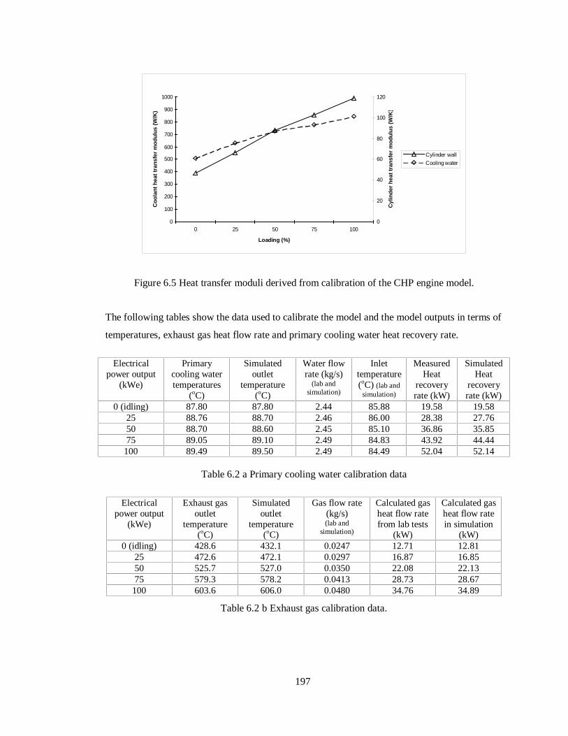
197
0
100
200
300
400
500
600
700
800
900
1000
0 25 50 75 100
Loading (%)
Co
ola
nt
hea
t tr
ansf
er m
od
ulu
s (W
/K)
0
20
40
60
80
100
120
Cyl
ind
er h
eat
tran
sfer
mo
du
lus
(W/K
)
Cylinder wall
Cooling water
Figure 6.5 Heat transfer moduli derived from calibration of the CHP engine model.
The following tables show the data used to calibrate the model and the model outputs in terms of
temperatures, exhaust gas heat flow rate and primary cooling water heat recovery rate.
Electricalpower output
(kWe)
Primarycooling watertemperatures
(oC)
Simulatedoutlet
temperature(oC)
Water flowrate (kg/s)
(lab andsimulation)
Inlettemperature(oC) (lab and
simulation)
MeasuredHeat
recoveryrate (kW)
SimulatedHeat
recoveryrate (kW)
0 (idling) 87.80 87.80 2.44 85.88 19.58 19.5825 88.76 88.70 2.46 86.00 28.38 27.7650 88.70 88.60 2.45 85.10 36.86 35.8575 89.05 89.10 2.49 84.83 43.92 44.44
100 89.49 89.50 2.49 84.49 52.04 52.14
Table 6.2 a Primary cooling water calibration data
Electricalpower output
(kWe)
Exhaust gasoutlet
temperature(oC)
Simulatedoutlet
temperature(oC)
Gas flow rate(kg/s)(lab and
simulation)
Calculated gasheat flow ratefrom lab tests
(kW)
Calculated gasheat flow ratein simulation
(kW)0 (idling) 428.6 432.1 0.0247 12.71 12.81
25 472.6 472.1 0.0297 16.87 16.8550 525.7 527.0 0.0350 22.08 22.1375 579.3 578.2 0.0413 28.73 28.67
100 603.6 606.0 0.0480 34.76 34.89
Table 6.2 b Exhaust gas calibration data.

198
The model calibration process described previously is useful if there is a limited quantity of
component data available. However, its major disadvantage is that the derived component model
parameters are not generic and must be re-calibrated for different primary cooling circuit flow
rates differ or another engine type requires simulation.
Analytical expressions for the calculation of both the cylinder wall and cooling water heat
transfer coefficients could have been used, however this would have required access to more
detailed engine performance information than was made available in the test data (i.e. cylinder
pressures, cooling circuit configuration, etc.).
Figure 6.6 shows the tuned engine unit model output against the test data for the most important
thermal parameters: exhaust gas temperature and cooling water outlet temperatures, both are
plotted against the engine work output.
6.2.2 Calibration of the PV model
One of the key features of the PV model, discussed in chapter 5, is the relationship between the
power output and temperature of the PV material, with the power output (in crystalline silicon
PV materials) generally decreasing with increasing material temperature. Recall that in chapter 5
a variable, σ, was used in the model of the PV material (equation 5.92). σ affects the power
output of the PV material through its influence on the calculation of the diode current (which
directly opposes the light generated current) and therefore influences the characteristics of the
power output. This variable must be obtained from laboratory testing of the PV material and
calibration of the parameter σ against the resulting test data.
The tuning method involved iteratively changing the value of σ until the slope of the PV
module power output against temperature (at constant incident radiation intensity) matched that
achieved in laboratory tests.

199
The laboratory tests on the PV modules were done using a solar simulator, consisting of an array
of tungsten lamps, which gave an irradiance level of 600W/m2. The modules were fitted to a
ventilated test rig from which temperatures, power output and heat recovery were measured.
Outputs from the tests included the combined efficiency of the PV module (i.e. the power output
plus recovered heat, the heat to power ratio and the power output to temperature characteristics.
More details of the tests and testing procedure are given in [11].
Figure 6.6 Some results from ESP-r’s simulations of PV panels against field trial data.
The other PV model parameters are obtained from manufacturer’s test data. Note this data is
measured at only one temperature, and so is of no use in determining temperature dependent
characteristics such as σ.

200
The photovoltaic special material model has been calibrated against numerous photovoltaic
module (panel) types, which incorporated both amorphous24 and crystalline solar cells, this is
reported on by Strachan [9, 10] and Clarke et al. [11] (refer to appendix 1 for a definition of
crystalline and amorphous photovoltaic materials).
The calibrated PV material models have also been integrated into ESP-r models of full scale,
outdoor PV facade test facilities [11, 12]. The output of the model was then compared to real
thermal and electrical data collected from experiments conducted using the test facilities. The
results from these field trial comparisons indicate that the predicted electrical output from the
calibrated PV component models agreed well with the collected data (see figure 6.7). The
equally important thermal performance of the ESP-r PV model also agreed well with the
experimental data. Note that figure 6.7 shows an apparent discrepancy between the time of the
measured and simulated values. This is probably caused by an unintentional time shift in the
simulation output data, which has gone uncorrected25.
6.2.3 Calibration of the Heat Exchanger Components
The cooling and gas water heat exchanger models were calibrated against manufacturer’s data.
However, this data covered the heat exchanger performance in limited steady state conditions
and therefore provided no test for the dynamic characteristics of the model. There is a general
lack of suitable data for use in plant component modelling verification, especially usable
dynamic data sets, against which plant component model transient performance can be tested.
24 In amorphous silicon materials the power output tends to remain constant with temperature. A best fit
with the laboratory data was achieved by setting σ to a high value (100), giving a flat power output to
temperature characteristic.
25 The phase shift is possibly due to the measurements being made in British summer time (BST), while
simulations are always conducted in Greenwich Mean Time (GMT).

201
Testing of each model’s transient performance was restricted to comparisons against simple
dynamic situations, and some inter-model comparisons. For the purposes of verification, Aasem
[6] has installed a facility within ESP-r that allows plant components to be subjected to simple
excitations such as step inputs in temperature and flow, ramp inputs in temperature and flow,
sinusoidally varying temperatures and flow, etc. The output from the excited component can
then be compared to an analytical solution of the dynamic process or the output from another
model of the component. One such model is shown in figure 6.8: this shows the representation
of the liquid-liquid heat exchanger, when modelled using the SIMULINK® simulation tool.
A series of analytical tests were carried out on the heat exchanger components and are reported
on in [7] and [8]. These tests also allowed errors and numerical instabilities in the components to
be identified and rectified.
Figure 6.7 The SIMULINK model of the liquid-liquid heat exchanger.
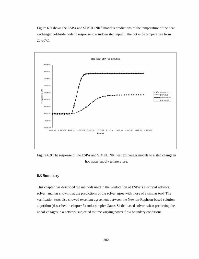
202
Figure 6.9 shows the ESP-r and SIMULINK® model’s predictions of the temperature of the heat
exchanger cold-side node in response to a sudden step input in the hot -side temperature from
20-80oC.
Figure 6.9 The response of the ESP-r and SIMULINK heat exchanger models to a step change in
hot water supply temperature.
6.3 Summary
This chapter has described the methods used in the verification of ESP-r’s electrical network
solver, and has shown that the predictions of the solver agree with those of a similar tool. The
verification tests also showed excellent agreement between the Newton-Raphson-based solution
algorithm (described in chapter 3) and a simpler Gauss-Siedel-based solver, when predicting the
nodal voltages in a network subjected to time varying power flow boundary conditions.
step input ESP-r vs Simulink
0.00E+00
1.00E+01
2.00E+01
3.00E+01
4.00E+01
5.00E+01
6.00E+01
7.00E+01
8.00E+01
9.00E+01
0.00E+00 2.00E+01 4.00E+01 6.00E+01 8.00E+01 1.00E+02 1.20E+02 1.40E+02 1.60E+02 1.80E+02 2.00E+02
Time (s)
Tem
per
atu
re (o
C)
simulink hot
ESP-r hot
Simulink cold
ESP-r cold

203
This chapter has also described the calibration of the CHP and PV, building-integrated energy
system component models. The calibration process involved the tuning of component parameters
against experimental data, so that the output of the models approximated that of measured
reality. The PV component model was further tested against experimental field trial data, with
encouraging results.
Both the solver and component models can therefore be used, with some confidence, in full-
scale, integrated models of building-integrated energy systems. The modelling of two such
systems is the subject of the next chapter.

204
6.4 References
1. Judkoff R, Wortman R, O’Docherty and Burch D, A methodology for validating building
energy analysis simulations, Report TR-254-1508, Solar Energy Research Institute,
Colorado, USA.
2. Gross C A, Power systems analysis, 1st Edition, Wiley, New York, 1979.
3. Weedy B M, Electric power systems, Wiley New York, 1979.
4. Bourdouxhe P, Grodent M, Lebrun J, Saavendra C, Cooling tower model developed in
toolkit for primary HVAC system Energy Calculation - part 1: model description and
validation using catalogue data, Proc. 4th International Conference, System Simulation in
Buildings, University of Liege, 1994.
5. CHP engine unit data from the Korean Institute of Energy Research (KIER).
6. Aasem E O, Practical simulation of air conditioning system in the transient domain, PhD
Thesis, University of Strathclyde, 1994.
7. Smith A C, Validation of a cooling coil model, BEng Thesis, University of Strathclyde, 1996.
8. Granger G, Evaluation of HVAC component models for energy simulation, BEng Thesis,
University of Strathclyde, 1996.
9. Strachan P A, Calibration of RMS95 modules using data from ITW Stuttgart, Preliminary
Energy Systems Research Unit Report, University of Strathclyde, 1997.

205
10. Strachan P A, Calibration with PST semi-transparent PV modules, Energy Systems
Research Unit Report, 1998.
11. Clarke J A, Hand JW, Johnstone CM, Kelly N J, Strachan P A, The Characterisation of
photovoltaic-integrated building facades under realistic operating conditions, Proc. 4th
European Conference on Solar Energy in Architecture and Urban Planning, Berlin, March
1996.
12. Clarke J A, Johnstone C, Strachan P and Bloem JJ, Ossenbrink HA, Thermal and power
modelling of the Photovoltaic facade on the ELSA building ISPRA, 13th Photovoltaic Solar
Energy Conference, Nice, 1995.

206
Chapter 7 - Modelling and Simulation of Building-Integrated
Energy Systems: Examples
7. Introduction
This chapter describes how the theory and model development of the previous chapters is
brought together to facilitate the key objective of this thesis: the simulation of the thermal and
electrical aspects of building performance, specifically the simulation of building-integrated
energy systems. Two exemplars are presented in this chapter, which demonstrate the capabilities
of an ESP-r model, augmented with a power flow network, in the analysis of such integrated
thermal/electrical systems. These exemplars are:
• a small sports centre incorporating a combined heat and power unit, supplying both the
electrical system and the hot water services;
• a factory building with a photovoltaic facade which supplies power to the building and from
which heat is recovered.
It must be emphasised at this point that the models and simulations presented in this chapter are
not intended to portray a design exercise: the current electrical modelling capability installed
within ESP-r is as yet prototypical and is not suitable for this function. The main functions of
these exemplars are to demonstrate how a model incorporating the thermal and electrical
domains is constructed and to illustrate the capabilities of an integrated simulation.
7.1 Modelling Integrated Systems in ESP-r
The building-integrated energy systems described in this chapter are some of the more
complicated models that can be defined in ESP-r: they incorporate various energy subsystems,
with very different time-constants. The modelling of such varied and stiff systems (i.e. with

207
elements of varying time constants) is perfectly suited to ESP-r’s flexible, modular approach to
both model definition and simulation.
7.1.1 The Definition of Integrated Models in ESP-r
Chapter 2 described how, in ESP-r, the complete building is modelled using a number of
integrated constituents: attributed polyhedral zones, which describe the form and fabric of the
building, and a series of superimposed networks, which describe the building’s energy
subsystems. In a dynamic simulation both the zones and networks are combined with real
climate data, time-varying internal thermal gains and detailed control information, forming a
single mathematical description of the building and its environment.
Each constituent of the building model can be thought of as a ‘layer’, with each layer adding
functionality and detail. The requirements of a particular simulation will dictate the form and
complexity of the model, with extra layers being added by the modeller as need requires. For
example, the most basic energy simulation would involve only one layer in a model, e.g. the
geometry and fabric of the building. If more functionality were required, this layer would be
augmented with air flow, CFD, plant and electrical networks, etc. The following table describes
the functionality added by the various constituents of an ESP-r model.
Model Constituent Functionality Typical Uses
the essential model “core”:
building fabric, climate,
occupancy, idealised ventilation
and infiltration
basic fabric thermal energy flows,
air, surface and fabric
temperatures, ‘free floating’
environmental conditions driven
by climatic and internal
excitations, daylight factor
calculations, solar distribution
overheating and summer comfort
analysis, basic lighting studies

208
+ zone based control logically and temporally
controlled heating and cooling
input to the zones and fabric
control strategy testing,
heating/cooling loads, plant
sizing, lighting control,
heated/cooled floor and ceiling
models
+ shading and insulation, blind/
shutter control
solar gains control, external and
internal solar shading
passive solar studies, location of
thermal mass, external shading
device studies, more detailed
overheating analysis
+ more detailed fabric modelling:
3-D conduction, non-linear
material properties, special
materials
three dimensional conduction,
detailed fabric thermal and non
thermal (i.e. electrical energy)
flows, advanced materials
thermal bridging, detailed floor
heat flows, phase change
materials, photovoltaics,
advanced glazing studies
+ air flow network pressure driven air flow and
ventilation, inter-zonal air flow
and moisture transport, detailed
fan models
natural and forced ventilation
studies, detailed overheating
analysis, passive/ambient cooling
strategies, e.g. night flushing
+ CFD air velocities and momentum,
temperature distributions,
air/surface boundary layer
information
detailed forced and natural
ventilation studies, convective
heat transfer coefficient
calculations, displacement
ventilation modelling, detailed
heating/cooling studies, atria
airflow patterns, etc.
+ moisture flow fabric moisture transport, surface
moisture absorption/evaporation,
interstitial condensation analysis,
mould growth prediction and

209
moisture storage analysis, rain water penetration,
desiccant material studies
+ plant detailed, component-based plant
descriptions, component
temperatures and energy flows
basic, uncontrolled plant
operation
+ component level control local component-based control
loops, logically and temporally-
based component operation
detailed air conditioning systems
modelling, control strategy
analysis, etc.
+ hot water flow network pressure driven hot water flows,
detailed pump models
detailed hot water services
modelling
+ hybrid components power generation component
models, lighting and small power
load electrical details
basic electrical energy flows and
demand calculations, basic supply
and demand analysis
+ electrical network real and reactive power flows
electrical energy flows, losses,
grid connection, power factors,
electrical transmission, system
voltages and current flows
detailed supply and demand
analysis, power systems
modelling, building-integrated
energy systems modelling,
renewable energy systems
modelling, grid import/export
+ global control strategies supervisory-level control, control
hierarchy, simulation-based
control
modelling of BEMS, global
control strategy modelling: peak
heat and power demand
management, controls systems
conflict resolution, etc.
Table 7.1 The added functionality from different layers of an ESP-r model.

210
Depending upon the requirements for a simulation, modellers have the choice of which of the
constituents listed in table 7.1 to use in their model, this allows great flexibility in both the types
of system that can be modelled and the level of detail to which they are defined. The modeller
can describe a building and its systems abstractly and then add more detailed layers as required.
It should be kept in mind that the larger and more detailed the model, the greater is the data input
requirement on the modeller. It is also worth noting is that as more detailed layers that are added
to the model the more expert knowledge is required from the modeller (i.e. knowledge of plant
modelling and HVAC systems or knowledge of power systems for power flow modelling).
Hence two important limiting factors on the eventual form of a model are the information
available to the modeller and the expertise of the modeller or design team.
However using a layered, modular problem description somewhat alleviates the problems
described above as the simulation model can evolve with a design, with the model gradually
acquiring more details as they become available (reducing the data input burden). Also, certain
elements of the model may be defined in more or less detail, depending on whether expert
knowledge is or is not available. This flexible approach to the problem definition is made
possible by the consistent application of the control volume in the description of every
constituent of the building model. Hence, while the model can be constructed from many
different and diverse layers (e.g. moisture flow, electrical networks, air flow networks, etc.) each
layer is based on the same elemental components: control volumes. Therefore, when the
constituents of the building model are connected together, they form a consistent mathematical
description of the building, no matter what the systems describe or the variation in the level of
detail throughout the model.
7.1.2 Simulation of Integrated Models
ESP-r’s modular simultaneous solution method is perfectly suited to complement the program’s
flexible approach to model description; it can be tailored to suit the constituents of any particular
model. As mentioned in chapter 4, the solution of the integrated system is achieved using a
unified simultaneous solution process. This is constructed from several coupled solvers, each of

211
which processes a particular energy subsystem of the model in an efficient manner and at a
frequency suited to the time constant of that particular element of the model. For example, the
plant, flow and electrical networks are usually processed at a high frequency, to suit their rapid
fluctuations in state, while the building fabric, with a longer time constant and more gradual
changes of state, can be processed at a more appropriate low frequency.
The examples that follow demonstrate the layer based modelling approach and the subsequent
use of the modular simultaneous solution process in the simulation of the integrated model.
7.2 Example 1: Combined Heat and Power in a Sport Centre
In this example, the modelling of a small sport centre is described. The building itself consists of
five main areas: a reception, changing rooms, a gym, the main sports hall and a plant room at the
rear of the building. Heat and power are provided by a small-scale combined heat and power unit
(CHP) integrated into the electrical services and the hot water services.
The loads that the hot water services feed include a heating coil in a mechanical ventilation
system, which heats the supply air to various zones in the centre, and a hot water calorifier,
which links to the domestic hot water services. The plant system is controlled so that the
combined heat and power unit will run as a lead boiler, supplying the base heating load of the
building during its opening hours. The major electrical loads in the building are the lighting
system, which is subject to daylight control, and the rotational loads (fans and pumps) in the
plant system. The electrical system of the building is three-phase a.c. and draws power from both
the CHP unit and a grid connection.
7.2.1 The Form and Function of the Model
In the modelling of this CHP-based energy system, the primary objective is to examine the
interactions between the energy supply from the CHP unit and the demand in the building. It is
therefore necessary to model both the CHP system and the building, particularly its heat and

212
power loads, in detail. The elements of the model required to do this are described in the
following paragraphs.
Figure 7.1 The ESP-r model of the sport centre.
exploded view
radiance viewstandard view

213
7.2.1.1 The Building Geometry and Fabric
Five thermal zones are used to model the geometry and fabric of the building (figure 7.1), which
has a total floor area of 2520m2 and an internal volume of 23,500m3. The building is steel
framed with an inner layer of block work, insulation and an outer layer of facing brick. The roof
is constructed from aluminium sheeting, backed with an insulating layer. The fabric of the
building is modelled using multi-layered constructions. Note that the definition of the building
geometry also allows the calculation of the daylight factors necessary for the simulation of the
lighting control system.
The lighting system is modelled as a hybrid load in each zone, with both the electrical and
thermal characteristics being described. The total thermal and real power load for the lighting
system is taken as 12W/m2. The lights in the building are an inductive load and are therefore
modelled with the lagging power factor of 0.95. The lighting control in the building assumes the
lighting in each zone (except the reception where lighting is uncontrolled) is arranged in three
banks running parallel to the glazed exterior sections of the building envelope. Each bank of
lights has its own daylighting sensor as shown in figure 7.2. When the sensed daylighting level
rises above a user defined lux set point, the lighting controlled by the sensor is dimmed or
switched off. Note, the form of daylight calculation and control used in these simulations is
idealised, Clarke and Janak [2] describe more complex lighting simulations which utilise both
ESP-r and the RADIANCE26 lighting analysis program.
The thermal loading from occupants inside the building is modelled using a time varying
sensible and latent heat gain to each zone.
26 Developed by Lawrence Berkeley Laboratories, California.

214
Figure 7.2 The lighting control layout in the main hall.
7.2.1.2 The Plant and Fluid Flow Networks
The plant network for the building describes both the hot water services and the mechanical
ventilation system. The hot water services comprise three 35kW boiler units feeding a hot water
calorifier and the air-heating coil of the ventilation system. A CHP hybrid thermal/electrical
component (described in the previous chapter) is connected in parallel with the boiler units, this
has a total heat output of 75kW at full load, and real electrical power output of 36kW at a
lagging power factor of 0.9.
The plant network is augmented with two separate flow networks, which describe the air flow in
the mechanical ventilation system and the hot water flow in the hot water services. Infiltration
and ventilation in the thermal zones are also modelled with the air flow network. The flow
inducing components, fans and pumps, are modelled in both the plant and fluid flow networks.
The flow components are augmented with electrical data; all are three-phase inductive loads
with a lagging power factor of between 0.75 and 0.8.
L
L
L
banks oflights
photo sensor
glazing

215
The plant network associated with the building model is shown in figure 7.3.
Figure 7.3 The sport centre’s plant network incorporating the CHP unit.
T T
T
T
air handling
unit
heat exchanger
CHP unit boilerscalorifier
extract fan
heating coil
warm air tothe zones
extracted air

216
Figure 7.4 The fluid flow networks.
fromsupplyfan
toextractfan
to zones
fromzones
fluidflownode
fluid flowconnection
air flowconnection
hot waterflow path

217
7.2.1.3 Control
The majority of the control associated with the model is contained in the plant network. Firstly,
the boilers and CHP network are controlled on the hot water return temperature (as described in
[3]) using a series of on/off control loops. The set points are arranged in such a way that the CHP
unit operates as the lead boiler, with the three boiler units acting, incrementally, as backup when
required. The CHP unit shuts off when the return temperature rises above 90oC or according to
time control. The air temperature in the sports centre is maintained between 19oC and 23oC by
proportionally varying the flow rate of hot water through the heating coil using a 3-port diverting
valve. Similarly, the hot water supply temperature from the calorifier is maintained at between
50-60oC by varying the supply flow-rate from the CHP and boilers, again using a diverting
valve. The plant system is time-controlled such that it operates during the centre opening hours
and a pre-heat period: this corresponds to an on period between 6.00 a.m. and 11.00 p.m., with
an unconditional off period outside these hours. The described control loops are superimposed
upon the plant network of figure 7.3
7.2.1.4 The Electrical Network
As has been indicated throughout this thesis, the electrical network is a critical constituent of the
building model, linking both the loads and CHP unit together and also linking the building to the
outside electricity grid. The electrical network of the model describes the building’s three-phase
distribution system and transports the power produced by the CHP unit to the lighting, small
power and rotational loads distributed throughout the thermal zones, plant and flow networks.
The link to the external grid is used as the reference node in the solution of the electrical network
(see section 3.3.1). The grid connection is bi-directional, when the loads in the building exceed
the generated output of the CHP unit power is drawn from the grid. However, when surplus
power is generated by the CHP unit, it is exported to the grid, which acts as an infinite source or
sink for electrical power. The electrical network for the sports centre is shown in figure 7.5. The
connections between the nodes in the network are three-phase cables, the nodes in the network
represent cable junctions or distribution points for electrical power.

218
Figure 7.5 The electrical network for the sports centre.
7.2.2 Simulations with the Model
An example simulation with the integrated model is conducted over the course of a winter
design week, 9-15th of January, using climate data from the Kew 1967 standard data set,
considered typical of climate conditions in the United Kingdom.
The modelling of the sports centre requires the use of several of ESP-r’s solvers: the building
solver, the plant solver, the fluid flow solver and the electrical network solver. These are used to
process systems of differing time constants. In this case the plant and electrical networks will
change their states rapidly, in the course of a few seconds. The air and surface layers of the
thermal zones will have a time constant of a few minutes, while the deeper fabric layers will
change their temperature over the space of a few hours. To cope with the stiffness of this
problem, variable frequency processing is employed, with the building zones solved every 15
minutes time and the plant, flow and electrical networks solved every 15 seconds. The high
three-phasecable
gridconnection
CHP unit
pumps
fans
reception lightsand small powerloads
gym lightsand smallpower loads
hall lights
changingarea lights
electricalnetwork node

219
frequency of processing on the plant and flow networks is necessary to capture the dynamics of
the changes in the state of the plant system and its associated effects on the plant control loops.
The electrical network must be processed at the same frequency, as any change in the state of
power consuming components in the plant network will have an effect on the electrical system
state. Processing at the same frequency allows these power consumption fluctuations to be
captured in the power system solution.
7.2.3 Typical Output from the Simulation
The following collage shows the spectrum of results data that can be recovered from the
simulation of the integrated system. It should again be stressed that these results are intended to
be indicative of the capabilities of an integrated simulation and are not the outcome of a design
exercise.

220
.
CHP coolant temperatures
0102030405060708090
9 10 11 12 13 14 15time (days)
tem
per
atu
re (
oC
)
Exhaust gas HE outlet
Engine jacket HE outlet
Heating output (kWh)
2046
4063
4063
8400
boiler 3 boiler 2
boiler 1 CHP
Import/export of power
-8000
-6000
-4000
-2000
0
2000
4000
9 10 11 12 13 14 15Time (Days)
Rea
l/Rea
ctiv
e P
ow
er (
W/V
A)
(+ve
imp
ort
-ve
exp
ort
)
Real
Reactive
Lighting real power demand
0
2000
4000
6000
8000
10000
12000
14000
16000
18000
9 10 11 12 13 14 15
Time (days)
Po
wer
(W
) changing
gym
main hall
entrance
Figure 7.6 Samples of results obtained from the integrated CHP simulation

221
Analysis of the results from this illustrative simulation showed that the total heating energy
supplied by the CHP unit was 8280kWh. The heating system maintained an average daytime
temperature of 19.7oC in the main hall. The total real power consumption of the building was
approximately 3129kWh, supplied at a lagging power factor of 0.89. Some 47kWh of this power
was required to make up resistive losses in the distribution system. The power output of the CHP
unit was 4033kWh, delivered at a lagging power factor of 0.9. Around 904kWh of real power
was supplied to the grid. Note that the first two graphs of figure 7.6 show the interaction
between the lighting control and the import/export of electricity; during the middle of the day
lighting power demand is drastically reduced, allowing the export of surplus power.
The paragraph above describes only a small quantity of the data that can be obtained from such a
complex simulation. Details of more information that could be extracted from integrated
simulations and its possible uses are given in the next chapter.
7.3 A Photovoltaic Facade on a Factory Building
This example looks at a photovoltaic facade integrated into the fabric of a factory building. The
facade feeds power into the building’s electrical system, while heat is recovered from air
warmed as it is drawn though the façade cavity. The model is loosely based on the ELSA
building at the EC’s research centre in Ispra, Italy [4].
The building itself consists of two main areas: a factory and an adjacent office area. Both
sections of the building are served by a mechanical ventilation system; this heats the incoming
air to the offices and factory, attempting to maintain a temperature of 20oC in both areas. The
warm air from the facade is passed into a heat exchanger, which heats the inlet air to the
mechanical ventilation system.
The electrical loads inside the building consist of rotational motor loads on the factory floor and
in the plant system, and also lighting loads in the factory and office zones.

222
7.3.1 The Form and Function of the Model
The main purpose of a integrated façade simulation is to quantify the useful recoverable heat and
power from the facade. The components of an integrated model required to do this are described
in the following sections. Again, as with the CHP exemplar, the function of the exemplar is
illustrative rather than a design exercise.
7.3.1.1 The Building Geometry and Fabric
The main sections of the building, the office and factory area are modelled using three thermal
zones. The total floor area of these zones is 1600m2 and they enclose a volume of 12500m3. The
building fabric is modelled using multi-layered constructions, and mainly consists of pre-
fabricated, insulated cladding.
The lighting and small power loads are modelled using zone load hybrid components, however
unlike the previous exemplar, the lighting in both the offices and the factory space is not
controlled and is switched on and off according to a time-schedule. Small power loads and
thermal gains from equipment and occupants are calculated using time-varying profiles.
The photovoltaic facade of the building is modelled in detail, using several thermal zones to
represent the facade construction: this consists of a ventilated photovoltaic module, mounted on
top of the insulated cladding of the building facade. In total, the facade is fitted with 420
photovoltaic panels, which are modelled using multi-layered constructions consisting of an outer
and inner glazing layer, a resin binder layer and an amorphous silicon PV special material layer.
The zones in the facade model represent the air gap behind the PV modules and allow the
explicit modelling of the important energy exchanges occurring inside and at the surface of the
facade: short-wave absorption, convective exchange, long-wave radiant exchange, conduction,
etc. The stacking of the facade zones (shown in figure 7.7) allows the modelling of the
temperature gradient as the air passes up through the facade.

223
Figure 7.7 The building and detailed facade model.
7.3.1.2 The Plant and Air Flow Networks
The basic building model is augmented with a plant network that describes the mechanical
ventilation system connected to the building. This heats the incoming supply air, such that
comfort conditions in both the offices and factory area are maintained. The heating and cooling
coil inside the ventilation system are supplied from hot water and chilled water systems
respectively (these are not modelled explicitly in this example). The plant network is also used to
the exploded PV facade indetail
standard view ofthe building
exploded view of thebuilding and facade
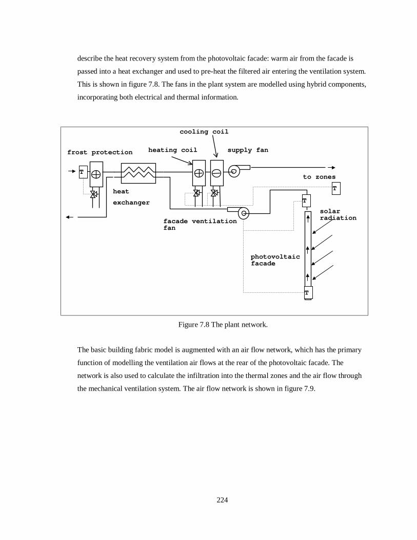
224
describe the heat recovery system from the photovoltaic facade: warm air from the facade is
passed into a heat exchanger and used to pre-heat the filtered air entering the ventilation system.
This is shown in figure 7.8. The fans in the plant system are modelled using hybrid components,
incorporating both electrical and thermal information.
Figure 7.8 The plant network.
The basic building fabric model is augmented with an air flow network, which has the primary
function of modelling the ventilation air flows at the rear of the photovoltaic facade. The
network is also used to calculate the infiltration into the thermal zones and the air flow through
the mechanical ventilation system. The air flow network is shown in figure 7.9.
photovoltaicfacade
heat
exchanger
heating coilfrost protection
facade ventilationfan
supply fan
to zones
T
T
T
T
solarradiation
cooling coil

225
Figure 7.9 The air flow network
7.3.1.3 Control
Control in the building is associated with the heating coil and fan components in the plant
network. The hot water flow rates through the heating and cooling coils are adjusted using a
three-port diverting valve such that the air temperature in the offices and factory are maintained
above 19oC. The control on the supply fan is time-based such that it provides fresh air to the
factory and offices between 8a.m and 5p.m. The fan drawing air from the PV facade is
programmed to operate when the temperature of the air emerging from the facade is 5oC warmer
than the ambient air temperature. This creates a reasonable energy flow across the heat
exchanger and between the two air streams. The component control loops are superimposed
upon the plant network of figure 7.9
air flow node
air flow path
NB stacked airflow nodes in thefacade model arerequired ifmodelling buoyancydriven air flow

226
7.3.1.4 The Electrical Network
As with the previous exemplar, the electrical network is used to model the three-phase
distribution system of the building and includes a connection to the grid, which is used as the
reference node. Power from the photovoltaic facade is fed into the electrical network, after
inversion. All the lighting and small power loads in the zones and the fan loads of the plant
system are connected to the network. This is shown in figure 7.10
Figure 7.10 The electrical network with input from the PV facade.
7.3.2 Simulation
A simulation can now be run to determine the recoverable heat and power from the facade when
subjected to a UK climate. The simulation is run for a spring week from 3-9th March, using the
standard Kew climate set. As with the sports centre, the different elements of the building are
three-phasecable
gridconnectionPV facade
fans
office lightsand smallpower loads
factoryarea lights
factoryareaequipment
electricalnetwork node
powerconditioning

227
processed at suitable frequencies, with the plant, airflow and electrical networks solved at 15-
second time intervals and the building processed at 10-minute time intervals.
7.3.3 Typical Results Output from the Simulation
Sample output from the simulation is shown in the results collage of figure 7.11.

228
Power Import
0
5000
10000
15000
20000
25000
30000
35000
40000
45000
0 24 48 72 96 120 144 168
Ti (h )
Po
wer
(W
)
RealReactive
Real Power Sources (kWh)
224
2342
pv output
imported
PV Power output
0
1000
2000
3000
4000
5000
6000
7000
0 24 48 72 96 120 144 168 192
Time (hours)
Po
wer
(W
)
Heating breakdown
0
200
400
600
800
1000
1200
factory offices
Hea
ing
en
erg
y (k
Wh
)
conventional heating
heat from facade
Figure 7.11 Sample of results obtained from the integrated PV facade

229
Over the simulation period the power produced by the facade totalled 224 kWh, while the useful
heat recovered totalled 608 kWh. The combined efficiency of the facade was 31%, the total
heating energy consumption of the building was 1455 kWh, while 2342.4 kWh of electrical
energy was consumed in the office and factory areas. This was supplied at a lagging power
factor of 0.88. 9.4% of the real power demand was supplied by the facade with the remainder
drawn from the grid.
Again, the information given in the preceding paragraphs is only a small fraction of that
available from the integrated simulation.
7.4 Summary
This chapter has described the modelling of two buildings using ESP-r, both of which
incorporate a building-integrated energy system. Using the components and electrical solver
developed in this thesis, both the thermal and electrical systems of the buildings were modelled
and simulated. Some sample results from these simulations were presented. These two
exemplars have been installed for use on the ESP-r system for training purposes in the modelling
of integrated systems.
The building-integrated energy systems models described in this chapter are but one use of the
capabilities of the ESP-r system augmented with an electrical network and hybrid
thermal/electrical modelling components. More potential uses are discussed in the next chapter.

230
7.5 References
1. Clarke J A, Energy simulation in building design, Adam Hilger, Bristol, 1985.
2. Clarke J A and Janak M, article in IBPSA News, Spring 1998.
3. Energy Efficiency Office Best Practice Program, Guidance notes for the implementation of
small scale packaged combined heat and power, HMSO, 1989.
4. Clarke J A, Johnstone C, Strachan P, Bloem J J and Ossensbrink H A, Thermal and power
modelling of the Photovoltaic facade on the ELSA building Ispra, 13th Photovoltaic Solar Energy
Conference, Nice, 1995.
7.6 Bibliography
Santamouris M, Asimakopolous D N (editors), Energy conservation strategies for sports centres,
vol 2: case studues, European Commission Directotate General for Energy Save Programme,
1996.
Energy Efficiency Office Best Practice Program Report, Remote monitoring of second
generation small-scale CHP units, New Practice Report No. 41, 1992.
Energy Efficiency Office Best Practice Program Report, CHP in a medium sized hotel, New
Practice Report NP/30, 1991
Energy Efficiency Office Demonstration Scheme Report, Combined heat and power in a
University Hall of Residence, Final Report, ED/206/228, 1988.

231
Chapter 8 - Review and Conclusions
8. Introduction
This chapter reviews what has been achieved in this thesis and also looks ahead to how the work
undertaken may be improved upon. Further research opportunities in the field of integrated
thermal and electrical modelling are discussed.
8.1 Review
This thesis has described a means of simulating the building’s electrical energy flows as part of
an integrated analysis of the entire building energy system.
The need for the integration of electrical energy flows into building energy simulation was
brought about by a desire to model building-integrated energy systems and also by a general
realisation that electrical power flows had been overlooked in building simulation. Thinking in
terms of the building as an energy system, electrical energy flows is equally as important as their
heat energy equivalent; therefore any complete model of the building must include them.
While a means to model the electrical energy flows is a useful addition for many aspects of
building simulation (i.e. BEMS modelling, lighting studies, etc.), this thesis has concentrated on
electrical power flow modelling within the context of the modelling of building-integrated
energy systems. These systems produce high-grade electrical and low-grade heat energy for the
building; thus the modelling of electrical energy flows is required. The two examples of such
systems described in this thesis were small-scale combined heat and power and photovoltaic
building facades. Both of these technologies are cleaner (and in the case of CHP more efficient)
sources of heat and power than the alternative of local hot water boilers coupled with electricity
supplied via the grid.

232
The design and analysis of building-integrated energy systems is complicated because
interactions with the building must be taken into account: the thermal interaction with the
building fabric, electrical demand and supply profiles, the influence of occupants, climate, plant
and control, and capacity limits imposed by components. It was stated previously that an
appropriate means of evaluating and designing such a system was through the use of a computer
simulation tool that could adequately simulate all the aforementioned thermal and electrical
interactions. This can be achieved by modelling the electrical power generation and distribution
systems with the rest of the building in a unified and integrated fashion.
Therefore, the objective defined for this thesis was to develop a prototype of such a tool, which
would enable the modelling and simulation of building-integrated energy systems through the
conflation of electrical systems modelling with building energy simulation. The program chosen
as the vehicle for this task was ESP-r [1].
At the commencement of the thesis, the ESP-r program could already model the complex
thermal interactions occurring between the building, the external environment, occupant
interactions, plant and control systems. The addition of a means to model the electrical energy
flows would allow the program to model both the thermal an electrical aspects of building
performance in an integrated fashion, whilst also laying the foundations of a tool for the
evaluation and design of building-integrated energy systems.
The steps required to achieve the objective of simulating the building’s electrical energy flows
and building-integrated energy systems modelling were defined as follows.
• The development of a means to describe and model the electrical energy system within the
building and a means of solving the electrical energy flows associated with it.
• The integration of this model of the electrical system into the ESP-r simulation program,
enabling the simulation of the electrical energy flows in the context of an integrated, whole
building simulation.

233
• The development of component models for use in the simulation of electrical and building-
integrated energy systems.
• The testing of the component models and electrical network solution technique.
• The development of exemplar applications to illustrate the use and capabilities of the thermal
modelling program augmented with an electrical modelling capacity.
The following sections summarise how the steps outlined above have been implemented.
8.2 The Integration of Electrical Power Flow Model ling into ESP-r
8.2.1 Description of the Electrical System
Chapter 2 described how, in ESP-r, the fundamental means of modelling the entire building
involves describing the building and its HVAC systems as a collection of connected control
volumes. Chapter 3 extended the concept of the control volume to encompass the modelling of
the building’s electrical system. This was described using a network, consisting of a set of
electrical control volumes coupled together by electrical conductors. The description of the
electrical system as a network was consistent with the means of describing other energy
subsystems in ESP-r, such as plant, air and moisture flows.
The concept of an electrical network proved amenable to the description of different types of
electrical systems; application of the network approach to three-phase and single-phase
alternating current, direct current and mixed systems was outlined in chapter 3.
8.2.2 Solution of the Electrical Power Flows
Solution of the electrical energy flows in the network was achieved by deriving, for each control
volume, two non-linear power flow balance equations for the real and reactive power flows. The

234
simultaneous solution of the resulting set of balance equations allowed the calculation of the
electrical network’s state variables (such as voltage) and the electrical power flows. A Newton-
Raphson iterative solver was developed to perform this task. The network solution requires that
boundary conditions, in the form of power drawn from and injected into the electrical network,
were known.
8.2.3 Integration into ESP-r
The power flow boundary conditions provided the means to integrate both the electrical network
and the solver into ESP-r, as they are calculated using the building model’s electrically driven
components (e.g. fans and pumps) and any building-integrated power generation (e.g. façade-
integrated photovoltaic components). These constituents of the building are also associated with
thermal phenomena (e.g. fluid flow) and so serve as a means to couple the electrical and thermal
networks.
The integration of the electrical solver into ESP-r’s modular simultaneous solution approach for
the whole building model was detailed in chapter 4; this enabled the electrical network to be
solved simultaneously with the other constituents of the building model.
8.2.4 Electrical Conductor Component Models
The component models of electrical conductors, which link the control volumes of the electrical
network together, were developed in chapter 5. Models of three phase and single-phase electrical
conductors and transformers were described. The impedance characteristics of these component
models were used in the formulation of the power flow balance equations for the electrical
network.
8.2.5 ‘Hybrid’ Component Model Development
The concept of the ‘hybrid’ component was introduced in chapter 4 and related models were
derived in chapter 5. These provided the means of translating the electrically driven thermal

235
phenomena occurring in the building model to the power flows required for the solution of the
electrical network. For example, a hybrid fan component, driving air around an HVAC network
model would draw the energy required to induce that flow from the electrical network.
Hybrid components were also developed for the modelling of building-integrated energy system
components: a combined heat and power unit and a ‘special material’, which could be used to
model both amorphous and crystalline photovoltaic components.
8.2.6 Verification
Chapter 6 described how the electrical network solver has been subjected to a series of
verification tests. In these tests the performance of ESP-r’s electrical solver was compared to
that of another power flow solution program. Both were used to model various test networks and
gave almost identical results.
Chapter 6 also described how the parameters of the CHP and photovoltaic special materials were
calibrated using laboratory data. Two heat exchanger models, developed for use with the CHP
model, were subjected to simple thermal excitations and their output compared against
analytically derived solutions and against other models; there was close agreement between all
of the models and the analytical solutions. Further tests of the photovoltaic model showed that
its predictions agreed well with experimental data taken form field trials.
8.2.7 Demonstration
Finally, two detailed exemplar applications were described in chapter 7. These were developed
with the aim of demonstrating the extended capabilities of ESP-r with respect to the modelling
and simulation of thermal and electrical energy systems in buildings, particularly building-
integrated energy systems. Both models are available on-line within ESP-r for use in the training
of users.

236
8.3 Suggestions for Future Work
The work undertaken in this thesis represents only the first step in the integration of electrical
systems modelling within building simulation. The electrical modelling capability integrated into
ESP-r as part of this thesis is only a prototype, which can be improved and expanded upon.
Some suggestions for this and possible further uses for integrated thermal/electrical modelling
are described in the following paragraphs.
8.3.1 Improvements to ESP-r and the Power Flow Solver
8.3.1.1 Three-phase Unbalanced and Mixed-Phase Systems
The capability of the electrical power flow solver currently installed in ESP-r is limited to the
modelling of balanced three-phase, single-phase and direct current power systems. The ability to
model unbalanced three-phase and mixed phase systems, as described in chapter 3, remains to be
implemented.
8.3.1.2 Improved Solver Integration Using Control
With the addition of global control strategies and electrical systems modelling into ESP-r [2],
there now exists the possibility for the development of electrical demand management control in
ESP-r. Recall that electrical demand management was discussed in chapter 4 as a means of
further coupling the electrical solver into ESP-r’s modular simultaneous solution method.
8.3.1.3 Load Models
ESP-r is currently equipped with hybrid component models of most of the major electrical loads
in the building: fans, pumps, small power loads and lighting. However this list is not yet
complete. Components such as compressors in refrigeration plant, vertical transportation loads
(i.e. lifts) and cooling towers must be added to ESP-r’s databases.

237
8.3.1.4 Detailed Rotational Load and Generator Models
The current hybrid rotational load models, described in chapter 5, are somewhat simplistic in
that both the rotational dynamics and a detailed equivalent circuit model of the electric motor are
not included. The addition of these two elements into more detailed fan, pump and generator
models would allow the modelling of transient, electro-mechanical effects such as power surges
and voltage drops during motor start-up and supply frequency variation.
8.3.1.5 More Realistic Representation of Small Power Loads
The representation of small heat and power loads (e.g. computers, faxes, televisions, etc.) in
simulation programs requires further investigation. Currently, the temporal variation of these
loads is represented by simplified, time-dependent profiles. There is a need for the development
of stochastic methods for the calculation and generation of more realistic electrical demand (and
thermal loading) profiles, particularly for larger buildings, which have large populations of these
small loads.
8.3.2 Uses for Integrated Thermal/Electrical Modelling
This thesis has described the application of electrical power flow modelling in the context of the
modelling of building-integrated energy systems. However, the network-based approach used to
model these systems is applicable to any type of electrical system, not just localised power
generation. Hence, the scope for modelling combined thermal and electrical systems is large.
Situations where the modelling of both the building’s thermal and electrical systems could be
beneficially deployed are outlined below.
8.3.2.1 Control
Perhaps the richest area for exploitation using integrated thermal and electrical modelling lies in
the field of control. The addition of electrical power flow modelling adds a new range of

238
variables (voltage, power flow, current, etc.) around which new control laws can be developed.
The example of a generator voltage controller has already been given in chapter 5.
Another example of where control could be applied in the power generation process is in
optimising the efficiency of inversion from a PV façade. If multiple inverters are used in this
process the number of active inverters can be controlled so that each operates at high loading and
high efficiency: inverters can be switched on or off, using a controller, as the power output from
the façade rises and falls with time.
As mentioned in chapter 4, control can be used to represent electrical safety devices such as
fuses and switches, which act to cut off the electrical supply to overloaded system conductors.
Also, if minimum and maximum operating voltages are incorporated into the hybrid components
attached to the electrical network, control could be used to model the effect of these
component’s safety devices, shutting them down if the operating limits are exceeded.
Further developments in interaction between energy pricing (especially electricity pricing),
demand, increasing flexibility in the electricity market and controls may play an increasingly
important role in the energy supply to buildings. For example, one system already operational in
France [3], uses the price of electricity to affect the control and electrical energy consumption of
domestic heating systems. The temperature set point of the system is reduced at times of high
electricity prices, which also coincides with periods of peak demands. Such tariff-responsive
building controls may well become reality in the UK commercial and domestic sectors. Building
simulation tools equipped with an electrical modelling capability may be used in the simulation
of this from of energy demand management.
Finally, returning to building-integrated energy systems, integrated simulation could be used in
the testing and development of advanced control algorithms, which match the demand of the
building to the supply of the integrated generation system. Such a system would be responsible
for making most efficient use of heat and power, minimising energy usage conflicts (e.g.
between lighting, daylighting and cooling), scheduling energy storage, limiting energy demand

239
and controlling energy supply. In effect, the control described here would be a global energy
management system, managing both the supply and demand of energy in a building.
If the advanced control systems mentioned above are to be designed correctly, it will be
necessary to model the interactions between the building’s electrical system and its energy and
environmental performance. The explicit representation of the electrical system in an integrated
model is therefore vital.
8.3.2.2 Autonomous Renewable Energy Systems
Integrated thermal and electrical modelling can be extended to the simulation of all scales of
energy systems, including larger-sized systems, which consist of more than one building and
power generation source; an autonomous renewable energy system is one such example. The use
of a building simulation tool in the modelling of renewable energy schemes is discussed in [4]
and power flow modelling is applied to the modelling of a wind energy conversion scheme in
[5]. Note that in most large-scale renewable energy simulations, the electrical demand is
modelled as a simple profile. The advantage of including the building in a renewable energy
system model is that the heat and power demands are explicitly calculated, and will vary as
functions of time, climate, control and user interactions. For this size of model, the electrical
network describing the building distribution system would become part of a larger network.
The generator voltage controller, discussed in chapter 5, would play an important part in the
simulation of autonomous energy systems. This control algorithm would be required to maintain
the voltage levels throughout the system as the supply from the connected renewable sources and
power demand vary with time and environmental conditions. Note that voltage control is only
possible if the electrical network of the system is modelled explicitly. This form of control could
also be used in the regulation of back-up generators, with the back-up capacity being switched
on as supply voltage drops with increasing load.

240
8.3.2.3 Electrical Systems Design
Currently, building simulation programs are used in the design and evaluation of the fabric and
environmental systems in buildings. The inclusion of a model of the electrical system opens up
possibilities for some aspects of electrical systems design to be accomplished within the context
of a building simulation. Examples include estimating the loading on cables, the balancing of
phase loading in larger buildings and the sizing of capacitor banks for power factor correction.
Note that if more detailed, dynamic electro-mechanical models of electrical equipment are
integrated into ESP-r (see section 8.3.1.4), the sizing of cables, fuses and switches could also be
undertaken within an integrated energy simulation, through the calculation of peak transient
loads in the relevant network elements.
8.4 Perspective
With the addition of electrical systems modelling into a building energy simulation tool, the
modeller now has the ability to perform a total evaluation of the energy and environmental
performance of a building, encompassing all the important energy flows: high grade electrical
and low grade thermal. Total building energy analysis will become increasingly important as
buildings increase in complexity, incorporating more advanced materials, technologies and
control and, as more stringent environmental performance criteria force designers to improve the
performance of their creations. This improvement in performance will be required both in terms
of energy consumption and occupant comfort.
Part of the solution towards improving the performance of the complex entities that are buildings
is through the increasing use of technology in their design. One of the problems in the building
design process has being a reluctance and fear on the part of designers and engineers to explore
and encourage modern design techniques such as simulation. This conservatism has maintained
a somewhat primitive approach to the design of what is a complex energy system and has
contributed to the poor performance of many of the buildings in existence today.

241
However, simulation too, must evolve to improve the accuracy and realism of modelling, and
also to take advantage of the ongoing advances in computing technology and applications. To an
extent this has happened, with simulation entering areas that were, until recently, untouched or
regarded as too complex to explore. For example, the capabilities of the ESP-r tool have been
expanded in recent years to include such diverse functionality as microscopic thermofluid
simulation [7,8], fabric moisture flow [9] and mould growth prediction [10].
While many areas of simulation remain to be fully developed and explored, it is hoped that the
work undertaken in this thesis is a small step in the continuing evolution of building simulation.

242
8.5 References
1. Clarke J A, Energy Simulation in Building Design, Adam Hilger, 1985
2. MacQueen J, The modelling and simulation of energy management control systems, PhD
Thesis, University of Strathclyde, Glasgow, 1997
3. Private communication with Giles Guyon, Électricité de France, 1998
4. Clarke J A, Evans M E, Grant A D and Kelly N J, Simulation tools for the exploitation of
renewable energy in the built environment: the EnTrack-GIS System, Proceedings of
Building Simulation `97, Prague, Czech Republic, 1997.
5. Kariniotakis G, Stavrakakis G, Nogaret E and Bordier M, Advanced modelling and
identification of autonomous wind-diesel power systems. Application on the French island
Desirade, Proceedings of the European Community Wind Energy Conference, Lübeck-
Travemünde, Germany, 1993.
6. Evans M S, Kelly N J, Modelling active building elements using special materials, Energy
Sysyems Research Unit Technical Report 95/18, University of Strathclyde, Glasgow.
7. Negrao C O R, Conflation of computational fluid dynamics and building thermal simulation,
PhD Thesis, ESRU, University of Strathclyde, Glasgow.
8. Clarke J A, Dempster W M and Negrao C O R, Predicting indoor air flow by combining
network approach, CFD and thermal simulation, Proceedings 16th AIVC Conference, 1995.
9. Nakhi A E, Adaptive construction modelling within whole-building dynamic simulation, PhD
Thesis, University of Strathclyde, Glasgow 1995.

243
10. Clarke J A, Johnstone C M, Kelly N J, McLean R C, Nakhi A E, Development of a
simulation tool for mould growth prediction in buildings, Proceedings Building Simulation,
Prague, 1996.

244
Appendix 1 - Photovoltaic Technology Review
A. Introduction
Photovoltaic materials produce electrical power from sunlight. The basic component of
photovoltaic power conversion is the solar cell. The amount of electrical energy produced is
dependent on the intrinsic properties of the solar cell and the availability and intensity of solar
radiation.
A.1 Solar Cells
Solar cells are most commonly fabricated from silicon, however other materials such as
cadmium and gallium may also be used. Silicon is a semiconductor material that is tetravalent,
i.e. group IV of the periodic table. If silicon is doped with ions from a group III material it
becomes an acceptor (p-type), when doped with a group V material it becomes a donator (n-
type). The p-type material is said to have a surplus of holes (rather than a deficit of electrons).
The most common solar cell is basically a p-n junction, where the p-type (positive) and n-type
(negative) materials are doped semiconductor(s). The p-n junction is a boundary in a
semiconductor material where a region of electron depletion neighbours a region of electron
surplus. A region of opposing charge is present in the areas of p and n-type materials (see figure
A.1) which are adjacent to the junction. This is known as the depletion region. In a state of
thermal equilibrium an electrostatic potential exists in the depletion region, which prevents
electrons diffusing from the n-type to the p-type material.
Four types of silicon semiconductor device are in use: monocrystalline, polycrystalline, thin film
polycrystalline and amorphous. Monocrystalline silicon has a highly ordered atomic structure
and cells made from it have the highest photovoltaic conversion efficiencies (18%).
Polycrystalline silicon consists of many crystalline grains; the conversion efficiency of a solar
cell manufactured from polycrystalline silicon is around 13%. Thin film polycrystalline devices

245
have a lower efficiency (11%). Amorphous silicon has a random atomic structure and solar cells
constructed from this form of silicon have a conversion efficiency of around 6-8%. The
conversion efficiency of amorphous PV materials tends to decay over time.
Figure A.1 A p-n junction
A standard solar cell is typically cut from a large ingot of monocrystalline or polycrystalline
silicon and is typically between 200 and 400 microns thick. The thickness of the wafer is largely
determined by the manufacturing process, however a minimum thickness of around 100µm is
required to ensure that the majority of the incident above-band-gap photons (defined in section
A.1.2.3) are absorbed. The wafer has metallic grids deposited on each side, which act as
electrical contacts and allow current liberated by sunlight to flow away from the cell.
Thin film amorphous silicon cells are created using an amorphous, silicon-hydrogen (Si-H)
alloy, which has a much greater ability to absorb photons than crystalline silicon. The
semiconductor material used in the cell can therefore be much thinner (e.g. 1µm). The normal
process of production is sputtering of the Si-H alloy onto a substrate. Common substrates
include glass and metals. The Si-H alloy is doped with phosphorous and boron to create n and p-
type materials respectively.
-+
+++
--
-- +
n-type material(electron surplus)
p-type material (holesurplus)
depletion regionsolar cell
246
Thin film crystalline silicon is created by precipitating the growth of a thin silicon layer on top
of molten, saturated solution of tin and silicon. This is done through controlled cooling. The
resulting layer is 2-3 µm thick. Texturing of the surfaces of a cell constructed using thin-film
silicon ensures that the path length of light through the cell is up to 20 times the cell thickness
(due to multiple reflections), thus ensuring that most of the incident photons are absorbed.
A.1.1 Solar Cell Physics
The following section provides a condensed review of solar cell physics and also explains the
basis for the characteristic equations of the photovoltaic special material of chapter 5. For a
comprehensive view of solar cell operation and photovoltaic systems the reader is referred to
standard texts such as [1]. Note this section only deals with simple p-n junctions in a single layer
of semiconductor (homojunction). Heterojunction cells (i.e. junctions of two different
semiconductor materials) are not discussed. Multijunction cells are discussed in section A.1.2.3.
In order for a current to flow in the semiconductor material, electrons in the valence orbitals
(which form the bonds between the atoms) must be promoted to a higher energy level so that
they are capable of conduction. The energy required for this is achieved by the absorption of
photons of light. The amount of energy required for a valence electron to jump to this higher
energy level is known as the band gap energy, Eg. This is an intrinsic property of the material
(e.g. crystalline silicon has a band gap energy of 1.12 eV, while that of amorphous silicon is
around 1.75 eV). Liberation of the electron involves the transition of the electron from a ground
state to an excited state (capable of conduction).
Electrons at or around the ground state energy level are said to be in the valence band (the
energy level associated with valence electrons), while electrons at excited energy level are in the
conduction band. These energy levels are denoted by Ev and Ec, respectively. The band gap
energy is given by the difference between them.
E E Eg c v= − . (A.1)

247
The liberation of an electron can be also be achieved by thermal excitation.
The liberation of an electron creates a corresponding vacancy in the valence band known as a
hole. Electrons and holes are the charge carriers in the semiconductor material (i.e. the source of
electrical current). In p-type materials the holes are the majority carriers, while in n-type
materials electrons are the majority carriers.
A.1.2 The p-n Junction
The following section describes and explores the properties of the p-n junction in a
semiconductor material, firstly in a state of equilibrium, then exposed to an external potential
and finally acting as a solar cell (when exposed to a light source).
A.1.2.1 The Unilluminated p-n Junction
In a state of thermal equilibrium, the fraction of electrons in the conduction band is given by
equation A.2
n n E f E dEcE
E
c
v
= ′∫ ( ) ( ) (A.2)
′n E( ) is the number of quantum states per unit volume of material, and is given by the
expression
5.05.13 )2(4)( EmhEn −=′ π , (A.3)
where h is Planck’s constant (6.62×10⁻³⁴Js) and m is the mass of an electron (9.11×10⁻³¹ kg), E is
the energy level (eV).

248
f(E) is a function giving the probability distribution of electrons entering the conduction band
(and holes entering the valence band), which is described by the following expression.
f EE
kTc( ) exp= − −
µ. (A.4)
µ represents the Fermi energy (J), the apparent energy level from which the majority carriers in a
p or n-type material are excited into the valence or conduction bands respectively (see figure
A.2); k is the Boltzmann constant (1.38×10⁻²³J/K), while T is the temperature of the PV material
(K).
Substituting equations A.3 and A.4 into equation A.2 gives
n h m EE
kTdEc
c
E
E
c
v
= − −
−∫ 4 23 15 0 5π µ( ) exp. . . (A.5)
Evaluation of the integral in equation A.5 gives the following expression for nc.
n NE p p
kTc c
c= − −
exp( ) ( )µ
(A.6)

249
Nc is a temperature dependant property called the conduction band effective density of state [1].
Figure A.2 The electrostatic properties of a p-n junction.
Electrons thermally excited into the conduction band of the p-type material can flow freely into
the n-type material. The size of this current, I po− ( ) (A), is proportional to the number of
electrons in the conduction band of the p-type material, the constant of proportionality, α, the
value of which is dependent on the electron mobility and the gradient of the electrostatic
potential.
Energy
Potential
φ(p)
φ(n)
∆φ = e∆Eo
n-regionp-region
Ec(p)
Ev(p)
Ec(n)
Ev(n)
∆EoFermi energy
level µ

250
The generation current is given by
I p NE p p
kTo cc− =
− −
( ) exp
( ) ( )α
µ. (A.7)
In the n-type material, electrons in the conduction band must overcome the electrostatic energy
barrier ∆Eo (J). The fraction of electrons capable of surmounting this barrier is given by the
following equation.
n n NE n n E
kTc cc o( ) exp
( ) ( )=
− − −
µ ∆. (A.8)
Looking at figure A.2, the electrostatic potential barrier, ∆Eo , can be substituted with
E p E nc c( ) ( )− . The expression for the current flow from the electrons excited into the
conduction region of the n-type material can therefore be expressed in the following form.
I n NE p n
kTo cc− = ′
− −
( ) exp
( ) ( )α
µ. (A.9)
This current is known as the recombination current and flows in the opposite direction to the
generation current. Under conditions of thermal equilibrium α α= ′ . The net electron current in
the system is given by the addition of the p-type and n-type currents.
I I p I no o− − −= +( ) ( ) . (A.10)
A.1.2.2 The p-n Junction Subjected to an External Potential
Under isolated conditions there can be no imbalance of currents in the depletion zone and the
sum of the generation current and recombination current is zero. However, when a potential
energy barrier Eext is applied across the junction (caused by the parallel connection of an
external voltage) it is no longer in equilibrium and the generated and recombination currents no

251
longer equate. For a negative Eext , the potential barrier that the electrons in the n-region must
overcome is increased and the current I no− ( ) decreases exponentially. In this case the net
current I − approaches I po− ( ) . For a positive Eext the current I no
− ( ) increases exponentially
with the external potential. In both cases I po− ( ) remains unchanged, it being dependant upon
the small number of electrons thermally excited into the conduction band in the p-material. This
current is temperature dependent.
The Fermi energies within the p-n material change when the external potential is applied such
that they are no longer in equilibrium; the following equation applies.
µ µ( ) ( )p n Eext− = −∆ . (A.11)
Re-arranging equation A.11 to an expression for µ( )n and substituting into equation A.9 gives
the following expression for I no− ( ) .
I n NE p E p
kTo cc ext− = −
− − +
( ) exp
( ) ( )α
µ∆. (A.12)
Substituting equation A.7, this can be simplified to,
I n I pE
kTo oext− −= −
( ) ( )exp
∆. (A.13)
Substituting equation A.13 into equation A.10, the net electron current in the conduction band,
per unit volume of PV material, can now be expressed (for the non-equilibrium state):
I I pE
kTo oext− −= −
−
( ) exp
∆1 . (A.14)

252
For any p-n junction the flow of electrons is only possible if there is a corresponding flow of
holes. The excitation of an electron into the conduction band in both the p and n materials
creates corresponding holes. These hole currents, I po+ ( ) and I no
+ ( ) , can be expressed by a
similar set of equations as were derived for electron currents. Therefore, the total current I across
the p-n junction is a summation of the electron and hole currents:
I I Io o= +− + . (A.15)
The total current I, in a unit volume of PV material, is given by
I I pE
kText= −
−
( ) exp
∆1 . (A.16)
This is called the Shockley equation and characterises the p-n junction under unilluminated
conditions. The unilluminated current flow in the p-n junction is referred to as the diode current.
A.1.2.3 The p-n Junction Exposed to Light
As stated earlier, liberation of an electron from the valence band can be achieved by the
interaction of a photon with the electron. The jump from the ground state to the excited state
liberates one (and only one) electron-hole pair and requires the absorbed photon to have an
energy of
gEhv > , (A.17)
where h is Planck’s constant: 6.626x10⁻³⁴ Js and v is the frequency (Hz). If a photon has an
energy greater than Eg, it creates an electron-hole pair with an energy of greater than Eg,
however the excess energy is soon dissipated as heat. Obviously, photons with a frequency less
than Eg/h will not liberate an electron-hole pair. This creates a fundamental efficiency limitation
in all photovoltaic conversion devices: only a fraction of the photons absorbed in the

253
photovoltaic material will have a frequency greater than Eg/h (so-called above-band-gap
photons) and much of the energy from the above-band-gap photons is wasted as heat.
Note, stacking two or more different layers of thin film layers, each with different band gap
semiconductors, can increase the efficiency of photovoltaic conversion. Usually the top film is a
high band gap material, while the subsequent layers have sequentially lower band gap energies.
With this type of cell a greater proportion of the incident photons are captured. Also, photon
capture occurs in layers with appropriate band gaps; with high energy photons captured the
upper layer and the lower layers capturing the non-absorbed, lower energy photons which pass
through the preceding layer. This reduces the thermal losses from the capture of photons with
energy levels greater than the band gap.
Exposure of the p-n junction to light ends the state of equilibrium in the junction as a large
number of electron hole pairs are created as well as increasing the number of thermally
generated pairs. The photo-induced current, Is, flows in the opposite direction to the current
defined by equation A.16. The total current flow in a unit volume of PV material exposed to
light, across an external potential drop, is given by
I I I pE
kTsext= −
−
( ) exp
∆1 . (A.18)
The p-n junction exposed to light is in a ‘forward-biased’ condition, where the vast majority of
the electrons-hole pairs will be created through photon absorption so that
I I p I ns + >>( ) ( ) .
The value of Is is dependent upon the proportion of the incident light that has a frequency
capable of exciting electrons into the conduction band F(λ). Other factors which affect the level
of light current generation include the fraction of light, of wavelength λ, absorbed by the PV
material, 1-R(λ) (where R(λ) is the quantity reflected), the radiation intensity, q(W/m2), and the

254
intrinsic semiconductor material properties. Is can be expressed in terms of the spectral
response of the solar cell:
[ ]I qF R SR ds = −=
=∞∫ ( ) ( ) ( )λ λ λ λ
λ
λ1
0. (A.19)
The spectral response of the cell at a particular wavelength λ of incident light is defined as
SRI
qF Rsc( )
( )
( )[ ( )]λ λ
λ λ=
−1, (A.20)
where Isc is the measured current produced by the solar cell when exposed to light of wavelength
λ and intensity q. The spectral response is defined as the ratio of the number of liberated carriers
leaving the solar cell to the number of photons entering.
A.1.3 Cell Characteristics
The output of a solar cell depends upon several factors: the properties of the semi-conductor
material, the cell temperature (in the case of crystalline silicon cells), ‘light soaking’ effects (in
amorphous silicon cells) and the nature of the external loads the cell supplies. The combination
of these factors gives rise to the characteristic operating curves, of generated current against the
output voltage for the solar cell. Typical examples are shown in figure A.4.

255
Figure A.4 Characteristic I-V curves for a solar cell.
A.2 Photovoltaic Panels
The photovoltaic panel consists of a number of solar cells connected in a series and parallel
configuration. The cells are encapsulated in a tough rigid structure containing the electrical
contacts and circuitry required to remove the liberated electrons to an external circuit. The
current output of the panel is dictated by the number of parallel connected cell branches, while
the panel output voltage is determined by the number of cells connected in series.
The output of the PV panel is direct current (d.c.). As outlined in the previous sections, the
current magnitude is dependent upon many factors including radiation intensity, cell
configuration and connected load. The maximum power output of the cell occurs at the knee of
their characteristic I-V curve (figure A.4).
Current
(A)
Voltage (V)
Isc
maximumpowerpoint
increasingintensity ofradiation
Voc

256
A.2.1 Power Conditioning
To ensure that the panel operates at the maximum power point, and hence efficiency, the
maximum power point must be tracked, this is done by a dithering technique, where once every
few seconds the current from the cells is increased or reduced until the maximum power output
point is attained. The technique is known as maximum power point tracking. The maximum
power point tracker effectively acts as a pseudo load for the solar panel, the characteristics of
which are adjusted so that the cells in the panel operate at their maximum efficiency.
The d.c. power output of the PV panel or array of panels is suitable for such purposes as battery
charging or supplying a resistive load. However, if a.c. electrical components are to be supplied
with power and/or the PV system is connected to the grid (see section A.3.1), the power output
of the PV source must be inverted. Inversion involves the conversion of the d.c. output to a.c.
A device called an inverter is used to convert the d.c. output of the photovoltaic array to an
alternating waveform. Three types of inverter are in used: variable frequency inverters (used for
stand-alone pumping applications), self-commutating, fixed frequency inverters and line-
commutated fixed frequency inverters. Only the latter two types are suitable for use in building-
integrated PV systems.
Self-commutating inverters require paralleling control equipment to maintain a synthetic output
a.c. waveform at a frequency suitable for connection to the grid. Line commutated inverters
(e.g. a switch-mode, pulse-width-modulated inverter) use the grid current waveform as a
reference against which to invert the PV output current. Clearly, line-commutated inverters
cannot be used in stand-alone systems, as they cannot operate without a grid connection.

257
A.3 The Integration of PV into Buildings
A.3.1 Integration into the Building Fabric
European Commission and the UK Energy Technology Support Unit (ETSU) studies [2, 3] have
identified the integration of PV materials into the building structure as one of the most cost
effective means of utilising this form of renewable energy. The reasons for this are that capital
costs are reduced, due to fact that the PV is an integral part of the structure and hence the cost of
cladding and displaced materials is saved, while land and support structure cost are avoided and
transmission losses are minimised.
There are several methods of PV integration into the building structure, these are outlined in
figure A.4 and table A.1
Installation type Advantages Disadvantages
Stand-off mount good panel cooling support structure is required,penetration through structure forcable access, heavy wind loadingpossible
Direct mount building structure is arraysupport, cables not exposed,panels displace facade materials
cooling problems, poor access toterminals, corrosion problems inwet climates
Integral mount panel forms an integral part of thestructure, panels can be mountedinto structure in the same way asglazing, free access to wiring andterminals
provision of necessary internalair-circulation for coolingpurposes
Under-glass mount cheap and easy to install, easyaccess and good coolingperformance
reflection losses, supportstructure shading effects
Table A.1 Summary of the advantages and disadvantages of different PV panel mountings.

258
Figure A.4 Photovoltaic panel mountings for building integration.
The most common and suitable type of mounting for new-build is the integral mounting. Here
the PV panel forms part of the facade, with the PV panels having the same dimensions as the
facade glazing elements. Modern building-facade compatible PV panels are constructed of a
glass-resin-glass sandwich with the PV cells set between the outer glass layer and the resin. The
glass used in the panel is usually low iron, to cut down on absorption of the incident solar
radiation. The solar cells may also be treated with an anti-reflective coating, maximising the
amount of solar radiation absorbed by them.
A.3.2 Grid Connection of Building-Integrated PV
As was mentioned in Chapter 1, one of the attractions of building-integrated energy systems is
the possibility of exporting power to the grid. This section looks at the options for the grid
connection of PV facades and the export of (suitably conditioned) a.c. power. Note that the
discussion here is also applicable to CHP systems.
structuralpenetration
stand-offmounting
directmounting
air gap
integralmounting
buildingfacade
under-glassmounting
reflection
structuralpenetration
PV
PV
PV
PV

259
A key issue in grid-connected buildings is that of metering, as it effects both the mode of
operation and the economic feasibility of a PV (or CHP) system. Note, issues relating to power
quality and safety are out-with the scope of this thesis. Two metering scenarios are possible: bi-
directional metering or single-metering. With bi-directional metering, power exported to the grid
will cause the meter to run backwards. Therefore, with this type of meter, the financial value of
electricity generated by the building-integrated system is the same as imported electricity.
However, this situation does not occur in the UK, where single metering is required: one for
exported power and one for imported power. The price paid for the exported power is less than
that charged for imported power (typically exported power has 1/3 the value of imported power
[4]). In this situation it is therefore economic to use all generated power within the building to
offset imported power. This results in most UK building-integrated PV systems being designed
to meet only internal building loads.
A.3.3 Heat Recovery from PV Facades
One of the problems with the integration of PV materials into the building structure is the low-
efficiency and high cost of the photovoltaic elements. Seasonal efficiencies of 12% have been
calculated for crystalline silicon panels (compared to flash test efficiencies of over 18% in some
cases). It is obvious that the operational efficiency falls short of that obtained in the laboratory
[5]. This lower efficiency results from several factors. Incident radiation intensities are usually
lower than the test values of 1000 W/m2 as atmospheric absorption of the solar spectrum reduces
the available solar radiation below this value. Also, the incident radiation is often not
perpendicular to the plane of the façade containing the PV arrays, further reducing the intensity
on the cells. Cell temperatures are often higher than the laboratory test values of 25oC, so that
the diode current, which opposes the light generated current, is higher than in test conditions,
reducing the output current.
The result of the lower operational efficiencies of PV arrays is that their payback period
becomes longer and they become less financially attractive to building owners and designers.
One method of boosting the operational efficiency of the PV facade is to recover heated air from
the rear of the panels. This boosts the efficiency of the facade in two ways. Firstly, recovered

260
heat can be fed into the building during the heating season (effectively the facade acts as a solar
combined heat and power system) secondly, the cell temperature is reduced, increasing the
electrical efficiency of the array.
The effect of the recovery of heated air from the rear of the facade is to greatly increase the
efficiency of the PV facade. Simulations have indicated combined efficiencies of up to 44% are
possible during the heating season in some climates [5]. The efficiency of the facade system will
be greatest when all the heat can be of use in ventilation pre-heat, or direct heating. The
temperature of the air recovered from the back of the panels can be as high as 60oC.
The direct displacement of building heating energy consumption due to façade heat recovery and
the resulting (slight) increase in electrical output act to improve the economic viability of
building-integrated PV.

261
A.4 References
1. Buresch M, Photovoltaic Energy Systems, McGraw-Hill, New York, 1983.
2. Taylor E H, Review of Photovoltaic Power Technology, ETSU, HMSO, London, 1990.
3. Photovoltaic Technologies and their Future Potential, Thermie OPET Publication, CEC DG
XVII,1993.
4. Simons A, Building-Integrated Photovoltaic Systems, Session 2: Technical Aspects of BIPV,
CREST Technical Paper, Loughborough University, 1998.
5. Clarke J A, Hand J W, Johnstone C M, Kelly N J and Strachan P A, The Characterisation of
photovoltaic-integrated building facades under realistic operating conditions, Proc. 4th
European Conference on Solar Energy in Architecture and Urban Planning, Berlin, March
1996.
A.5 Bibliography
Fonash S J, Solar Cell Device Physics, Academic Press, New York, 1981.
Hu C and White R M, Solar Cells - From Basic to Advanced Systems, McGraw-Hill, New York,
1983.
Markvart T (editor), Solar Electricity, John Wiley, Chichester, 1998.
Mohan N, Udehand T M and Robins W P, Power Electronics: Converters, Application and
Design, John Wiley and Sons, New York 1989.

262
Palz W, Vianello V, Bonalberti E and Riedel D (editors), First E.C. Conference on Solar
Collectors in Architecture - Integration of Photovoltaic and Thermal Collectors in New and Old
Building Structures, Proceedings of the First International Conference, Venice, Italy 3-5 March
1983.
Partain L D (editor), Solar cells and their applications, John Wiley and Sons, New York, 1995.
Sorensen B, Renewable Energy, Academic Press, London, 1979.
Twidell J and Weir T, Renewable Energy Resources, E & F N Spon Ltd., London, 1986.

263
Appendix B - Small-Scale Combined Heat and Power
Technology Review
B. Introduction
Small-scale Combined Heat and Power (CHP) is a well-established technology in the UK and
world-wide. The engine drives a generator, which produces power for the building electrical
loads, while waste heat from the engine is recovered to produce hot water for use in the building
services. CHP units vary in size from 18kWe (electrical output) to over 1 MWe and usual heat-
to-power ratios are in the region 1.75:1. The overall efficiency of a packaged CHP unit is in the
order of 80%. Typically, about 30% of the fuel energy is converted to mechanical work output ,
while around 50% of the remaining fuel energy is recovered as hot water. The energy flows
associated with a combustion engine small-scale CHP unit are shown in figure B.1
Figure B.1 CHP unit energy flow paths.
flue andcasing losses
engine unit
fuel supply(gas/diesel)
cooling waterheat exchanger
exhaust gasheat exchanger
cool waterreturn
hot watersupply
poweroutput
100%15%
60%25%

264
By the end of 1993 nearly 1000 units were operational in the UK producing 3000MWe [1]. The
current UK government strategy is to encourage a further 2000MWe of new CHP capacity over
the period 1995-2000.
B.1 The Components of a CHP System
The main components of a small-scale CHP system are as follows.
• the engine;
• the generator;
• the heat recovery system (cooling water and exhaust gas heat exchangers).
B.1.1 The Engine
The engines used in packaged CHP are usually spark-ignition gas or dual fuel engines, derived
from industrial or mass-produced automotive models. Larger CHP units may use a gas turbine,
but the principles of CHP operation remain the same. The most common fuels are biogas or
natural gas. Diesel is usually only an attractive fuel option if already used on site: it produces
appreciable quantities of particulate that tend to foul the exhaust gas heat exchanger.
Engine sizes for small-scale CHP systems can vary from around 25kWe output to very large
diesel or gas turbine units >500kWe. Generally, the engines run at a multiple of the grid
frequency (50Hz), e.g. 1500 rpm.
A typical internal combustion engine unit engine will run with a jacket temperature of 120oC and
an exhaust gas temperature of 650oC. The majority of heat is recovered from the exhaust gases.
The temperature at which the engine runs is dependent upon a number of factors including
engine speed and the fuel type.

265
The engine is required to supply a torque, Tm (Nm), to the generator. Under steady state
conditions (the conditions prevailing for the vast majority of the time) this torque is balanced by
an electrical counter torque, Te. With a constant engine speed the fuel consumption will vary
linearly with the torque requirement.
B.1.2 The Generator
The basic components of the generator are the rotor and the stator. The rotor is the component
driven by the mechanical torque from the prime mover, (i.e. the engine). The stator is a
stationary component that houses the field windings out of which the generated current flows.
The generators in packaged CHP units generally have a 3-phase alternating current output at
415V (line-line voltage), with a power output typically in the range 15kWe and upwards. Two
types of generators can be used on CHP units: synchronous and asynchronous.
Synchronous generators are self-excitating, i.e. they do not rely on an external power source to
energise the stator field windings. The magnetic field necessary for the induction of the current
flow in the stator windings is induced by supplying a d.c. excitation current to the rotor, this is
supplied via slip rings or brushes. The generated frequency is dependent upon the speed of
rotation of the rotor, ω, and N the number of magnetic poles on the rotor. The generated
frequency is given by the following expression.
fN= ωπ4
. (B.1)
The output of the synchronous generator is a complex power with a real and reactive component.

266
Asynchronous (or induction) generators can operate either as motors or generators and require
an external source (typically the grid) to provide reactive power for the creation of a rotating
magnetic field in the stator windings27. If the speed of the rotor is less than the speed of this
rotating field in the stator, i.e. ω ω< field , then the machine operates as a motor and real and
reactive power are absorbed. If an external force is applied to the rotor, causing it to rotate faster
than the rotating stator field such that ω ω> field , then the current flow in the stator windings is
reversed and real power flows out of the stator terminals. The induction generator still absorbs
reactive power to maintain the rotating stator field. The difference between the rotor speed and
the stator field speed is known as the slip. The rotor in an asynchronous generator will always
rotate at a greater speed than the synchronous speed when generating power. The amount of
power generated from the asynchronous generator is a function of the slip, this is discussed
further when control of the generator power output is considered.
B.1.3 Heat Recovery System
All CHP units recover heat from two main areas: the engine coolant water and the exhaust gases.
Heat outputs for small-scale CHP units range from 39kW to 1,200kW and are typically twice the
electrical output. The maximum operating water temperatures are roughly similar to low
temperature hot water (LTHW) systems at approximately 75-90oC.
Two types of heat exchanger are required on the CHP system: the jacket cooling water heat
exchanger and an exhaust gas heat exchanger. The cooling water heat exchanger is usually of the
shell and tube or plate variety, while the exhaust gas heat exchanger consists of banks of finned
tubes, containing the cooling water over which the exhaust gas flows at a temperature of 500-
27 Note that in synchronous generators the field rotates with the rotor, in asynchronous machines the field
rotates on the stationary stator as the currents in the stator windings change direction.

267
650oC. Around 60% of the heat transferred to the cooling water is recovered from the engine
jacket, with 40% recovered from the exhaust gas heat exchanger.
B.2 Control of CHP Systems
B.2.1 Temperature Control
Control of a CHP unit is applicable in two area: control of the thermal output of the unit and
control of the electrical output of the generator. Of the two, the control of the thermal operation
of the unit is more common and is crucial to the CHP unit’s efficient operation.
Thermal control of the unit is based on the heat demand with or without reference to electricity
demand and is similar to the control of a conventional boiler (temperature based). The normal
control strategy is to run the unit at full load for as long a period as possible, with the CHP unit
effectively running as a lead boiler in preference to the back-up boilers in the building’s heating
system. This ensures that the CHP unit runs for as many hours as possible during the day.
It is common to control the CHP on the hot water return temperature with the supply temperature
allowed to float, enabling the CHP unit to supply the maximum quantity of heat to the
circulating cooling water.
B.2.2 Control of Power Output
It is also possible to control the electrical output of the generator unit in relation to variation in
electrical demand. Control of the electrical output of both synchronous and asynchronous
generators is discussed below.

268
Figure B.2 Per-phase equivalent circuits of synchronous and asynchronous generators
Referring to the per-phase equivalent circuit of the synchronous generator (assuming balanced
operation), the complex power (VA) supplied to the system by the generator is
S VI= ′ . (B.2)
Apply Ohm’s law and replacing I in equation A2.2 gives
S VE V
X d= −
′. (B.3)
Noting that the terminal voltage V V= , the excitation voltage )sin(cos δδ jEE += and the
synchronous reactance X jXd d= (Ω). S can be expressed as
SVE
Xj
VE
X
V
Xd d d= + −
sin cosδ δ2
, (B.4)
RXe
Xm
Pm
VV
Xd
E
synchronousgenerator
asynchronous(induction)generator
statorvoltage
terminalvoltageterminalvoltage
terminalvoltage
synchronousreactance
I
Im
leakagereactance
stator and rotorresistance
I

269
where the real power output of the generator (equal to the mechanical power Pm supplied by the
CHP engine unit) is
PVE
X d= sinδ , (B.5)
and the reactive power output is given by
QVE
X
V
Xd d= −cosδ
2. (B.6)
It is possible to control both the real and reactive power output of the generator through two
separate control actions. Increasing the mechanical power, Pm (W), while keeping the rotational
speed of the shaft constant, will cause the real electrical power output, P (W), to increase, with a
small decrease in Q (VAR) and an increase in δ (rads). Increasing the magnitude of the
excitation voltage E will leave P unaffected, while increasing Q and decreasing δ.
In the asynchronous generator, changing the slip angle can control the output of real power. This
is achieved by increasing or decreasing the torque from the engine unit. Referring to the
equivalent circuit of the induction generator, the relationship between the mechanical power
output of the engine and the slip s is given by
o
om
sXR
REKsP
+=
2. (B.7)
Here K is a characteristic term for the generator, given in manufacturer’s data, as are Eo, which is
the terminal voltage at standstill. Xo is the magnetising reactance (Ω) at rotor standstill. The
reactive power consumption can be altered using a capacitor bank.

270
B.3 Connecting the CHP system into the Building Services
Two methods exist for connection of the CHP unit into the services, these being a series or a
parallel configuration. The series connection is the most often used when the CHP unit is
retrofitted to an existing installation. This is due to the fact that a series connection creates the
minimum disruption to the existing services. However a bypass must be installed to ensure that
flow from the CHP unit circulates when the boilers are closed down (i.e. in summer conditions).
The parallel connection is used when the entire boiler and CHP package is installed as new. Note
that the higher hydraulic resistance of the CHP unit means that it must be equipped with its own
pump. The parallel connection configuration is used in the CHP exemplar of chapter 5.
Figure B.3 Connection of a CHP unit to the hot water services.
B.4 The Viability of CHP
To asses the suitability of small-scale CHP at a given site, a detailed assessment of the site
energy demand must be undertaken. If the available heat load is not sufficient to allow the CHP
unit to operate for more than 4500 hrs/year it is unlikely that the scheme will prove financially
viable [2].
CHP
CHP
series connectionparallel connection
boilers boilersbypass
CHP pumpCHP pump

271
To achieve the required running time, the site must have a demand for hot water all year round.
Examples of this type of site include hospitals, offices, hotels and swimming pools. In addition
to these sites, research has indicated there are over 3,000 group housing sites, flats, old peoples
homes, hostels and sheltered accommodation which could benefit from CHP.
Generally the CHP unit is sized to meet the summer hot water requirement, plus a proportion of
the winter heating demand. The boilers supply the additional hot water requirement in winter.
B.4.1 Efficiency and Savings
This section discusses means of evaluating the efficiency and savings from CHP systems (this
can also apply to savings from photovoltaic facades), which can be used in the evaluation of
simulations such as the exemplars given in chapter 7.
B.4.2 Measures of Efficiency
There are many methods of gauging the efficiency of CHP plant, the most simple is the energy
utilisation factor (EUF), which is given by
EUFW Q
Fu
c= +
. (B.8)
This is the ratio of useful power and heat output to fuel input. The fuel consumption Fc can be
further defined as
FQ
IHR Ecc
cc c= +
η(B.9)
The fuel consumption in the above equation can be broken down into two components: the fuel
used for heating purposes and the fuel used for electricity production. The IHRc term is the
amount of fuel used (kW) per kW of power production. Substituting this back into equation B.8

272
gives another expression for the EUF in terms of the electrical output, heat output, combustion
efficiency and the incremental heat rate.
EUF
E
QIHR E
Q
c
c
c
c c
c
=+
+
1
1
η
(B.10)
Another measure of efficiency is the fuel energy savings ratio (FESR). This is the ratio of the
fuel used by the CHP unit to the fuel that would have been used by a boiler and traditional
generating plant to produce the same amount of heat and power:
FESRF F
Fs c
s= −
. (B.11)
Fs is the parallel generation fuel consumption (i.e. boiler plus power plant) and Fc is the fuel
consumption of the CHP unit. The fuel energy savings ratio is useful when determining the CO2
savings of CHP installation.
B.4.3 Financial Savings from CHP
The financial savings associated with CHP come in two possible forms. The first is the saving in
imported electricity while the second is the possibility of exporting generated electricity to the
grid. The unit value of electricity produced by the CHP system can be written in terms of any
sales or displaced purchases:
KE K E KED
Eejcs esj cd j
c=
+(B.12)
Ecs is the electricity produced by the CHP unit (kW) and exported to the grid at rate Kesj(£/kW).
Ecd (kW) is the displaced electricity at rate Kedj (£/kW). Note that Ecs + Ecd = Ec (the total amount

273
of electricity generated by the unit). The savings accrued from the CHP system are dependent on
the value of Kej and Kedj.
The general case is that Kedj> Kesj and connection to the grid for export purposes also carries a
charge. Hence, most UK CHP units supply electricity for displacement purposes only.

274
B.5 References
1. Combined Heat and Power Association, CHPA yearbook, CHPA publication, 1995.
2. Evans R D, Environmental and economic implications of small-scale CHP, ETSU, 1990.
B.6 Bibliography
Energy Efficiency Office, Good practice guide 1 - guidance notes for the implementation of
small-scale packaged combined heat and power, HMSO 1993.
Energy Efficiency Office, Good practice guide 3 - introduction to small scale combined heat
and power, HMSO 1990.
Emanuel P, Motors, generators, transformers and energy, Prentice-Hall, New Jersey, 1985.
Gross C A, Power systems analysis (1st Edition), John Wiley and Sons, New York, 1979.
Horlock J H, Cogeneration: Combined heat and power, Pergammon Press, Oxford, 1987.
Porter R W, Manstaniah K, Thermal-economic analysis of heat matched industrial cogeneration
systems, Energy, Vol. 7, No 2, 1982.