Water 2017, 9, 137; doi:10.3390/w9020137  www.mdpi.com/journal/water 

Article 

Tracer Experiments and Hydraulic Performance Improvements in a Treatment Pond 

Shang‐Shu Shih 1, Yun‐Qi Zeng 1, Hong‐Yuan Lee 1, Marinus L. Otte 2 and Wei‐Ta Fang 3,* 

1  Department of Civil Engineering, National Taiwan University, Taipei 106, Taiwan;   

uptreeshih@ntu.edu.tw (S.‐S.S.); yoj7230@hotmail.com (Y.‐Q.Z.); leehy@ntu.edu.tw (H.‐Y.L.) 2  Wet Ecosystem Research Group, Department of Biological Sciences, Department 2715,   

North Dakota State University (NDSU), P.O. Box 6050, Fargo, ND 58108‐6050, USA; 

marinus.otte@ndsu.edu 3  Graduate Institute of Environmental Education, National Taiwan Normal University, Taipei 116, Taiwan 

*  Correspondence: wtfang@ntnu.edu.tw; Tel.: +886‐939‐859‐399 

Academic Editor: David Sample 

Received: 17 November 2016; Accepted: 14 February 2017; Published: 20 February 2017 

Abstract: The treatment efficiency of a wetland constructed for nutrient removal depends strongly 

on  the  flow patterns and residence  times of  the wetland.  In  this study, a  tracer experiment was 

performed to estimate the residence time distribution and the hydraulic efficiency of a treatment 

pond with shallow and deep‐water areas. Rhodamine WT experiments revealed a non‐uniform flow 

pattern in the deep‐water area and an overall poor hydraulic efficiency in the wetland. To improve 

flow  uniformity  and  hydraulic  efficiency,  several  design  options  for  different  inlet–outlet 

configurations, flow rates, water depths, and emergent baffle additions were considered. The effects 

on hydraulic performance were investigated through mathematical model simulations. The results 

revealed  that  increasing  the  flow  rate  and  decreasing  the water  depth  slightly  improved  the 

hydraulic  performance,  whereas  changing  the  positions  of  the  inlet  and  outlet  produced 

inconsistent effects. The most effective improvement involved installing emergent baffles, with the 

number of baffles presenting  the  largest positive effect,  followed by  the width and  length of  the 

baffles. Long and thin baffles resulted in a uniform flow velocity field, a meandering flow path, and 

greater residence  times and effective volume ratios. The  installation of  two baffles  increased  the 

hydraulic efficiency to 1.00, indicating excellent hydraulic performance. The thin baffles occupied 

approximately 3.7%–6.3% of the deep‐water area and 1.9%–3.2% of the entire pond, indicating the 

potential for their practical application in limited land use regions. 

Keywords: pond; rhodamine WT; mathematical modeling; flow uniformity; hydraulic performance 

 

1. Introduction 

Wetlands are highly beneficial, and promote biodiversity by providing habitats for plants, birds, 

and insects that have an affinity for aqueous environments. Treatment ponds are one type of artificial 

wetlands designed to provide multiple functions [1–5]. Such ponds are widely used in urban areas 

for storm water management, ecological conservation, and pollution treatment [6]. Degradation by 

microorganisms and adsorption by plants are two of the primary mechanisms for pollutant removal 

and degradation  [7]. The overall effectiveness of both mechanisms  is dependent on  the  residence 

time, or  the  length of  time  that water and pollutants  are  retained  in  the wetland. The  treatment 

potential and efficiency of wetlands are usually related to the residence time of individual parcels of 

water within the wetland [8]. Wang and Mitsch [9] suggested that treatment could be improved by 

manipulating the hydraulic regime to improve hydraulic performance. Parameters such as the aspect 

ratio, bottom  topography, water depth, vegetation, baffles, and  inlet/outlet position can  influence 

wetland hydrodynamics and determine both the retention time and hydraulic efficiency [10–13]. It 

Water 2017, 9, 137  2 of 16 

has been  suggested  that hydraulic performance  could be  improved by allowing  the  flow  to pass 

uniformly through the wetland and avoiding short‐circuiting flows and dead zones [14]. 

Williams et al. [15] showed that ponds are the largest contributors to biodiversity, and supported 

more unique  species  than other  types of waterbodies,  such as  rivers,  streams, and ditches,  in an 

agricultural  landscape  in  southern England. A number of additional  studies have  confirmed  this 

finding  [16–18].  The  hydraulics  of  ponds  and  wetlands  can  generally  be  evaluated  through 

mathematical modeling  [19,20]  and  tracer  experiments  [21,22].  This  study  investigated  the  flow 

hydrodynamics, residence time distribution, and hydraulic performance of a treatment pond using 

tracer experiments and mathematical modeling. A well‐trained horizontal two‐dimensional model 

was employed to simulate flow conditions and tracer concentrations in several scenarios involving 

10 sets of flow rates, nine sets of water depths, nine sets of inlet and outlet locations, 14 sets of single 

emergent baffles, and six sets of two emergent baffles. 

2. Methods 

2.1. Study Area 

Approximately 10,000 agricultural ponds were present 100 years ago on the Taoyuan Plateau, 

northern Taiwan. Historically, farmers used these ponds to preserve water for rice paddy irrigation. 

Thus, agricultural ponds were distributed throughout the plateau and connected by irrigation ditches 

to form artificial, but semi‐natural, bird habitats [18]. The pond studied in this study is an agricultural 

pond  located  in  Taoyuan  County,  northern  Taiwan,  on  private  land  belonging  to  a  soybean 

processing company  (Figure 1). The  factory produces  large quantities of nutrient‐rich wastewater 

that could cause pollution and damage  the environment  if directly discharged  into  the creek. To 

prevent this discharge, the factory installed a treatment pond to treat the turbid and odorous soybean 

wastewater.  This  pond  was  originally  a  swimming  pool,  but  was  abandoned.  The  authors 

incorporated  the  pool  into  a  treatment  wetland  pond  to  treat  soybean  wastewater.  Previous 

published studies [23–25], on the wetland include architectural design concepts, field observations, 

and experiments. The pond was designed with a hydraulic retention time (HRT) between 28 days 

and 30 days. Most of the substrate in the pond was embedded concrete elements below ground. Thus, 

porosity could be neglected in subsurface flow although the soil bank may facilitate lateral exchange 

with groundwater. The upstream section of  the pond was designed  to hold shallow water with a 

meandering  flow. The downstream section  is a  large area of deeper, open water, and  it has been 

suggested that the hydraulic performance of this deeper section could be improved. The water depth 

of the upstream section is approximately 1.0 m, and that of the downstream section is approximately 

2.3 m. The  length and width of  the wetland are approximately 100 m and 35 m,  respectively.  In 

addition to the wastewater from the factory, the wetland receives clean water from Caoling Creek. 

The water and pollutants enter the wetland in the shallow‐water area and exit from the deep‐water 

area via a rectangular weir, which is designed to control the water depth of the wetland. 

Water 2017, 9, 137  3 of 16 

 

Figure 1. Location of  the  study area. The blue arrows  indicate  the  flow  inlet and outlet, and  the 

schematic shows the main flow direction. 

2.2. Tracer Experiments 

Tracers are used in a variety of environments, such as those involving aquifers, streams, rivers, 

estuaries, reservoirs, lakes, and wetlands [26]. Rhodamine WT, a fluorescent xanthene dye, has long 

been used as a hydrologic tracer in surface water systems [27], including rivers and wetlands [28]. 

Dierberg and DeBusk  [26]  compared  the  applicability of  rhodamine WT and  lithium  chloride as 

tracers in wetlands. Rhodamine WT has a recovery rate between 64% and 75%. As long as a complete 

concentration‐time  hydrograph  can  be  obtained,  an  integral method  can  be  used  to  analyze  the 

residence time distribution (RTD) curve and calculate hydraulic parameters. Rhodamine WT meets 

regulations and is easily detectable with a portable fluorescence detector at concentrations as low as 

0.01 μg∙L−1 [27,29–31]. Therefore, rhodamine WT was used as a tracer in the present study to observe 

the  flow and diffusion of contaminants  in  the water body. A 200 mL volume of  the  tracer with a 

concentration of 25,000 mg∙L−1 was instantaneously added at the pond inlet. At the outlet, variations 

in the tracer concentration were measured over time to obtain the tracer response curve and the RTD 

curve and to assess the overall hydraulic performance of the wetland. In addition, a rectangular weir 

was  installed at the outlet to measure the flow rate. A submerged underwater fluorescence meter 

(Cyclops‐7, Turner Designs, San Jose, CA, USA) and an automatic recorder were installed in front of 

this  weir  to  record  changes  in  the  tracer  concentration  every  30  min.  Three  different  sets  of 

experiments were conducted to assess three different flow rates (0.0026, 0.0011, and 0.0039 m3∙s−1) at 

the same water depth (2.0 m). 

2.3. Hydraulic Performance 

To assess the treatment efficiency and hydraulic performance of the wetlands, Persson et al. [11] 

presented a hydraulic efficiency equation: 

11  (1) 

Water 2017, 9, 137  4 of 16 

where ev is the effective volume ratio and N is the number of continuously stirred tank reactors (CSTR) 

in  series.  The  hydraulic  efficiency    can  be  categorized  into  three  levels:  (1)  good  hydraulic 

efficiency,  0.75 ;  (2)  satisfactory  hydraulic  efficiency,  0.5 0.75 ;  and  (3)  poor  hydraulic efficiency,  0.5. 

According to Thackston et al. [10], ev indicates the utilization of the effective volume ratio of a 

detention system: 

  (2) 

where tn is the mean residence time in [h], as shown in Equation (3), and tm is the nominal retention 

time in [h] calculated from the first moment of the tracer response curve [6]: 

  (3) 

where V is the volume of the pond in [m3] and Q is the flow rate in [m3∙s−1]. 

cdt

cdt

∑ c c2

∑ c c2

(4) 

where c is the tracer concentration in [μg∙L−1], t is the time of measurement [h], and tm is the mean 

residence time in [h]. 

Kadlec and Knight [32] suggested an alternative formula for calculating N based on differences 

in the time of the peak outflow concentration and the nominal retention time: 

  (5) 

where tp is the time of the peak concentration in the tracer response curve measured at the outlet of 

the pond in [h]. 

Chang  et al.  [14]  substituted Equations  (2) and  (5)  into Equation  (1)  to obtain  the hydraulic 

efficiency formula (Equation (6)), which  is used to estimate the hydraulic efficiency in the present 

study: 

  (6) 

2.4. Mathematical Model 

To determine the spatial distribution of the flow and the tracer concentrations of the free‐water 

area of the wetland, a horizontal two‐dimensional hydrodynamic and water quality transport model 

(TABS‐2) was developed. TABS‐2 consists of  two modules: RMA2 and RMA4. RMA2 and RMA4 

were implemented for water velocity and tracer concentration calculations. 

2.4.1. RMA2 Module 

RMA2 is a two‐dimensional depth‐averaged finite element hydrodynamic model for computing 

the water surface elevations and horizontal velocity components of the subcritical free‐surface flow 

field [33]. The governing equations of RMA2 pertain to mass and momentum conservation, as shown 

in Equations (7)–(9): 

∂∂

∂∂

∂∂

0 (7) 

∂∂

∂∂

∂∂

∂∂

∂∂

∂∂

∂∂

0  (8) 

Water 2017, 9, 137  5 of 16 

∂∂

∂∂

∂∂

∂∂

∂∂

∂∂

∂∂

0 (9) 

where  x  and  y  are  the  Cartesian  coordinates  of  the  horizontal  and  longitudinal  directions, 

respectively, in [m]; t is time in [s]; ρ is the water density in [kg∙m−3]; h is the water depth in [m]; u 

and v are the velocities in the x‐ and y‐directions, respectively, in [m∙s−1]; Exx, Eyy, Exy and Eyx are the 

eddy viscosity  coefficients  in  [Pascal∙s];  a  is  the  elevation of  the bottom  in  [m]; and τx and τy are 

external forces in the x‐ and y‐directions, respectively, in [m∙s−2]. 

2.4.2. RMA4 Module 

RMA4  is  a  finite  element water  quality  transport model  in which  the  depth  concentration 

distribution is assumed to be uniform [34], and its governing equation is given by Equation (10): 

∂∂

∂∂

∂∂

∂∂

∂∂

∂∂

∂∂

0  (10) 

where c is the tracer concentration in [μg∙L−1], Dx and Dy are turbulent mixing (dispersion) coefficients 

in [m2∙s−1], σ is the source/sink of the constituent in [μg∙L−1∙s−1], kc is the first‐order decay coefficient of 

the tracer in [day−1], and R(c) is the rainfall/evaporation rate. The first‐order decay coefficient, kc, was 

used in the model to simulate the non‐conservative behavior of rhodamine WT [35–37]. 

2.4.3. Determination of Parameters 

There are five parameters that must be determined in TABS‐2: (1) the roughness value, n, which 

was estimated from an empirical formula and set as 0.035–0.045 due to different vegetation; (2) the 

temperature, T, which was obtained from field measurements and ranged from 24 to 35 °C; (3) the 

eddy viscosity, E, the dispersion coefficient, D, and the decay coefficient, kc, which were determined 

via the parameter calibration and model verification process described in Section 3.2.1. 

2.4.4. Determination of Boundary Conditions 

The  TABS‐2 model was  developed  based  on  field  surveys,  including  surveys  of  the  pond 

topography,  flow  rate, water  surface elevation, and  tracer  concentrations. The  topography of  the 

pond was investigated using a TOPCON Total Station (GTS226, TOPCON, Tokyo, Japan) and was 

used to develop the fixed boundary of the RMA2 model. A rectangular weir was installed at the outlet 

to measure the flow rate using the weir formula. A HOBO Water Level Logger (model U20‐001‐01, 

Onset, Bourne, MA, USA) was installed in the deep‐water area to record the water stage every 60 

min. The investigated flow rates and water depths were entered as the upstream and the downstream 

boundaries of the RMA2 model. The pulse‐input concentration of the tracer described was set as the 

upstream boundary of the RMA4 model, as discussed in Section 2.2. 

2.4.5. Numerical Experiments 

After  parameter  calibration  and  model  verification,  several  numerical  experiments  were 

proposed and conducted. The effects of decreased water depth,  increased flow rate, and  installed 

baffles in the deep‐water area and alterations at the locations of the inlet and outlet were evaluated. 

Ten cases of different flow rates and nine cases of different water depths were investigated. The water 

depth was the same (2.0 m) in cases of different flow rates. Additionally, the flow rate was also the 

same (0.002 m3∙s−1) in cases of different water depths. Nine cases of different inlet and outlet locations 

were also investigated. The following inlets and outlets were tested: Case IO‐0 was the original site 

design (i.e., inlet and outlet located at the corners); in Case IO‐1, the inlet was located at the corner 

and the outlet at the boundary midpoint; and in Case IO‐2, the inlet was located at the corner and the 

outlet on  the diagonal. The  flow  rate  and water depth  for  the  cases of different  inlet  and outlet 

locations were set to constant values of 0.002 m3∙s−1 and 2.0 m, respectively. 

In addition, Shih et al. [6] and Chang et al. [14] suggested that the addition of emergent baffles 

could considerably alter the hydraulic efficiency in a deep‐water wetland. Therefore, several baffles 

Water 2017, 9, 137  6 of 16 

with different lengths, widths, and aspect ratios were modeled. The aspect ratio is calculated as the 

baffle length divided by the baffle width, whereas the length and width are defined as the distances 

parallel and perpendicular to the flow direction. Fourteen cases of placing a single baffle and six cases 

of placing two baffles were investigated. The flow rate and water depth for these cases were set to 

constant values of 0.002 m3∙s−1 and 2.0 m, respectively. 

3. Results and Discussion 

3.1. Tracer Experiments 

Three tracer conductance experiments were performed. Peak values of different concentrations 

were observed, and the findings were consistent to those of Bodin et al. [38]. In the first experiment, 

the highest peak tracer concentration (11.9 μg∙L−1) occurred at t = 76.5 h after introduction of the tracer. 

A second peak appeared at t = 100.0 h. Approximately 10 days after the beginning of the experiment, 

the tracer concentration returned to the baseline level (Figure 2a). In the second experiment, the peak 

value of 7.85 μg∙L−1 was measured at t = 98.0 h. On approximately the 11th day, the values returned 

to the baseline (Figure 2b). In the third experiment, a peak value of 10.0 μg∙L−1 was measured at t = 

75.0 h. On approximately the 8th day, the values returned to the baseline (Figure 2c). The effective 

volume ratios were estimated as 0.56 in Experiment No. 1 (Exp. 1), 0.25 in Exp. 2, and 0.26 in Exp. 3. The 

hydraulic efficiencies were calculated as 0.18 in Exp. 1, 0.02 in Exp. 2, and 0.05 in Exp. 3 (Table 1). The 

pond  exhibited  a  generally  poor  hydraulic  performance.  The  experiments  yielded  a  complete 

concentration hydrograph and, because rainfall did not occur during  the survey,  these data were 

used to adjust the parameters of the mathematical model. 

Table 1. Model validation by field measurements of hydraulic retention time, effective volume ratio, 

and hydraulic efficiency. 

Experiment  tn (h) tm (h) tp (h) ev  λ 

1 Field  239.6  134.2  76.5  0.56  0.18 

Model  239.6  135.8  66.5  0.57  0.16 

2 Field  860.3  169.4  98.0  0.25  0.02 

Model  860.3  211.6  90.0  0.25  0.03 

3 Field  354.8  90.6  75.0  0.26  0.05 

Model  354.8  135.1  68.5  0.38  0.07 

 

Water 2017, 9, 137  7 of 16 

a. Experiment 1‐ model calibration

b. Experiment 2‐ model verification

 

c. Experiment 2‐ model verification

 

Figure 2. Results of mathematical model validation: (a) measurements from Exp. 1 for model calibration; 

(b) measurements from Exp. 2 for the first verification; and (c) measurements from Exp. 3 for the second 

verification. The correlation coefficients (R2) were 0.83, 0.62, and 0.66. The eddy viscosity (E), dispersion 

coefficient (D), and decay coefficient (Kc) were determined to be 12, 0.012, and 0.21, respectively. 

0

2

4

6

8

10

12

14

0 50 100 150 200 250 300 350

Cn

cen

trat

ion

(μ

g L

-1)

Time (h)

measurement

simulation

E = 12D = 0.012kc = 0.21

R2 = 0.83 (p < 0.01)

0

2

4

6

8

10

12

14

0 50 100 150 200 250 300 350 400

Con

cen

trat

ion

(μ

g L

-1)

Time (h)

measurement

simulation

E = 12D = 0.012kc = 0.21

R2 = 0.62 (p < 0.01)

0

2

4

6

8

10

12

14

0 50 100 150 200

Con

cen

trat

ion

(μ

g L

-1)

Time (h)

measurment

simulatiion

E = 12D = 0.012kc = 0.21

R2 = 0.66 (p < 0.01)

Water 2017, 9, 137  8 of 16 

3.2. Mathematical Model Simulation 

3.2.1. Parameter Calibration and Model Verification 

The model simulations were compared to field observations of the tracer response curves (Figure 

2). Parameters such as  the eddy viscosity  (E), dispersion coefficient  (D), and decay coefficient  (kc) 

were  adjusted  from  experiment  1  (calibration)  and  determined  from  experiments  2  and  3 

(verification). The correlation coefficients  (R2) between  field  investigations and model simulations 

were  0.83,  0.62,  and  0.66,  and  they  indicated  significant dependence  between  the measured  and 

simulated results (p < 0.01). The simulated and measured tracer concentration values were consistent, 

except  for  the background  concentrations and  tracer  tails of all of  the  experiments and  the peak 

concentrations of experiments 2 and 3. The invalid tracer tails were due to transient storage, which 

was attributable to hyporheic exchange [28]. Although most areas of pond bed were embedded with 

concrete, other areas such as the pond bank exhibited possible signs of lateral hyporheic exchange 

through the bank (S.S. Shih, personal observations). Although the model simulations did not yield 

background and peak concentrations that were consistent with field observations, the key hydraulic 

parameters derived  from  the method of moments were not affected  [26],  suggesting  comparable 

values of effective volume  ratio and hydraulic efficiency  (Table 1). The  results  indicated  that  the 

mathematical model simulations yielded acceptable calculations of hydraulic performance. 

3.2.2. Flow Hydrodynamics and Hydraulic Performance 

The observed two‐dimensional horizontal distributions of the flow direction, flow velocity, and 

tracer concentrations are illustrated in Figure 3. The spatial distribution of the flow velocity was non‐

uniform and consistent with the results of previous tracer experiments [39]. The flow velocity ranged 

from 0.00005 m∙s−1 to 0.0001 m∙s−1 in the shallow‐water area and from 0.00001 m∙s−1 to 0.00008 m∙s−1 in 

the deep‐water area. The water depth ranged from 0.8 m to 1.2 m in the shallow‐water area and from 

1.2 m to 2.5 m in the deep‐water area. The Froude number ranged from 0.32 to 0.56 in the shallow‐

water area and from 0.12 to 0.39 in the deep‐water area, which indicated a subcritical flow condition 

in  the  entire  pond.  The  results  indicated  a  low  velocity,  deeper water,  and  non‐uniform  flow 

conditions in the deep‐water area relative to those in the shallow‐water area. The dead zones (i.e., 

areas with a  flow velocity below 0.00005 m∙s−1) occurred  in  the upper  right corner and  lower  left 

corner of the deep‐water area, which may have decreased the hydraulic performance by inhibiting 

water exchange with other zones. A region of short‐circuited flow (i.e., a region of high flow velocity) 

was observed from the lower right corner to the upper left corner of the deep‐water area, which may 

have  reduced  the  residence  time  and  flow  uniformity  and  thereby  decreased  the  hydraulic 

performance and treatment efficiency. The poor hydraulic efficiency resulted primarily from short‐

circuited  flow and  the presence of a dead zone  in  the deep‐water area. Hydraulically,  treatment 

efficiency  is  considered  satisfactory  as  long  as  the  system  is  well  mixed  and  the  physical 

characteristics are uniform across  the wetland perpendicular  to  the  flow  [40]. The poor  treatment 

efficiencies  of  suspended  solids were  detected  due  to  the  occurrence  of  short‐circuited  flow.  In 

addition, a low nitrogen removal rate was likely due to the dead zone in the deep‐water area. The 

results may be different for other pollutants, such as biochemical oxygen demand (BOD), for which 

adsorption does not occur. 

3.3. Changing the Flow Rate and Water Depth to Improve Hydraulic Performance 

3.3.1. Flow Rate 

Ten  cases  of  different  flow  rates were  investigated.  The  flow  velocity  and  flow  uniformity 

increased with  increasing flow rate. Based on  the  tracer response curves and RTD curve analysis, 

increasing the flow rate (from 0.001 m3∙s−1 to 0.010 m3∙s−1) decreased the nominal retention time (tn), 

mean residence time (tm) and time of peak concentration (tp) values. The effective volume ratio and 

the hydraulic efficiency increased with increasing flow rate. The increase in the flow rate exhibited a 

Water 2017, 9, 137  9 of 16 

positive linear relationship with the hydraulic efficiency (Figure 4). When the flow rate was increased 

to 0.010 m3∙s−1, the hydraulic efficiency increased to a satisfactory level (λ = 0.74). 

(a) Finite element mesh (b) Topography

(c) Flow direction (d) Velocity magnitude

(e) Water depth (f) Tracer concentration

Figure 3. (a) Finite element mesh; (b) bathymetry; (c) flow direction; (d) flow velocity; (e) water depth; 

and (f) tracer concentration distribution in the pond. 

 

Water 2017, 9, 137  10 of 16 

a. 

b. 

Figure 4. (a) Tracer concentration hydrograph and (b) hydraulic efficiency at the pond outlet across 

the entire pond for different flow rates. 

3.3.2. Water Depth 

Nine cases of different water depths were investigated. The flow velocity and flow uniformity 

increased with decreasing water depth. At shallower water depths, the difference between the mean 

residence time (tm) and the nominal retention time (tn) was reduced, which  increased the effective 

volume ratio. In addition, at greater water depths, longer mean residence time (tm) values and lower 

0

10

20

30

40

50

60

70

0 100 200 300 400 500 600

Con

cen

trat

ion

(μg

L-1

)

Time (h)

Q = 0.001 m³s⁻¹

Q = 0.002 m³s⁻¹

Q = 0.003 m³s⁻¹

Q = 0.004 m³s⁻¹

Q = 0.005 m³s⁻¹

Q = 0.006 m³s⁻¹

Q = 0.007 m³s⁻¹

Q = 0.008 m³s⁻¹

Q = 0.009 m³s⁻¹

Q = 0.010 m³s⁻¹

λ = 80.142Q - 0.025R² = 0.996

0.00

0.10

0.20

0.30

0.40

0.50

0.60

0.70

0.80

0.90

0.000 0.002 0.004 0.006 0.008 0.010 0.012

Hh

ydra

ulic

eff

icie

ncy

Flow rate (m3 s-1)

Water 2017, 9, 137  11 of 16 

effective volume ratios were observed, which resulted in a reduction in hydraulic efficiency. Water 

depth exhibited a negative linear relationship with hydraulic efficiency (Figure 5). By decreasing the 

water  depth  of  the  pond  outlet  to  1.4 m,  the  hydraulic  efficiency was  increased  to  0.30, which 

indicated  a  poor  hydraulic  level.  Decreasing  the  downstream  water  depth  yielded  slight 

improvements in the effective volume ratio and hydraulic efficiency. 

a. 

b. 

±

Figure 5. (a) Tracer concentration hydrograph and (b) hydraulic efficiency at the pond outlet across 

the entire pond for different water depths. 

 

0

5

10

15

20

25

0 100 200 300 400 500 600

Con

cen

trat

ion

(μg

L-1

)

Time (h)

h = 1.4 m

h = 1.7 m

h = 2.0 m

h = 2.1 m

h = 2.2 m

h = 2.3 m

h = 2.4 m

h = 2.7 m

h = 3.0 m

λ = ‐0.1378H + 0.4609R² = 0.921

0.00

0.05

0.10

0.15

0.20

0.25

0.30

0.35

1.0 1.5 2.0 2.5 3.0 3.5

Hyd

rau

lic e

ffic

ien

cy

Water depth (m)

Water 2017, 9, 137  12 of 16 

3.4. Altering Inlet and Outlet Locations to Improve Hydraulic Performance 

Nine  sets of different  inlet and outlet  locations were  investigated. The  results  indicated  that 

changing the  location of the outlet did not significantly  improve flow uniformity or the hydraulic 

efficiency (Figure 6). When moving the inlet from the upper right corner to the midpoint (Cases IO‐3 

to IO‐5), the hydraulic efficiency slightly increased. By contrast, when the inlet was moved from the 

upper right corner to the lower right corner (Cases IO‐6 to IO‐8), the hydraulic efficiency was reduced. 

Changing the inlet and outlet positions yielded inconsistent effects on the hydraulic efficiency. 

IO-0 (λ = 0.39) IO-1 (λ = 0.39) IO-2 (λ = 0.39)

IO-3 (λ = 0.42) IO-4 (λ = 0.43) IO-5 (λ = 0.43)

IO-6 (λ = 0.23) IO-7 (λ = 0.23) IO-8 (λ = 0.23)

Figure 6. Spatial distribution of the flow velocity in the treatment pond for different inlet and outlet 

configurations. Case IO‐0 represents the current conditions of the pond, and the other cases represent 

scenarios for improving the hydraulic efficiency. The blue arrows indicate the flow inlet and outlet. 

The hydraulic efficiency is shown in parentheses according to the name of each scenario. 

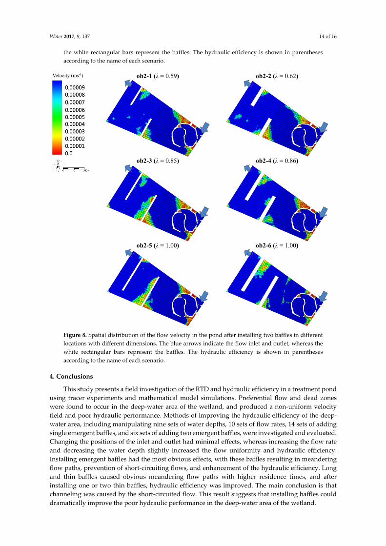
3.5. Adding Emergent Baffles to Improve Hydraulic Performance 

This hypothesis considered determining whether poor hydraulic performance was related to the 

low removal rate of pollutants in deep‐water areas of the downstream section of the pond. Fourteen 

different placements of a single emergent baffle were  investigated. The baffles were placed  in the 

same locations in the deep‐water area. The results of flow field simulations are shown in Figure 7. 

Case  ob1‐0  represents  the  current  conditions,  and  the  other  cases  represent  the  experimental 

scenarios. When the baffle width was 35.8 m, the hydraulic efficiency increased to 0.63 (Case ob1‐5), 

whereas increasing the length did not produce significant improvements (Case ob1‐11 and Case ob1‐

14). The width of the baffle was found to be crucial for improving the hydraulic efficiency. The best 

hydraulic efficiency of 0.68 was achieved by adding a single baffle. The placement of two emergent 

baffles was also considered, for which six cases were investigated (Figure 8). Cases ob2‐5 and ob2‐6 

performed  the  best,  followed  by  cases  ob2‐3  and  ob2‐4.  Cases  ob2‐1  and  ob2‐2  had  the worst 

performance.  The  placement  of  two  baffles  positively  increased  the  hydraulic  efficiency  to  1.00 

because  it caused  the waterway  in  the deep‐water region  to meander and effectively reduced  the 

Velocity (ms-1)

Water 2017, 9, 137  13 of 16 

dead zone area and short‐circuited flow. In the case of short‐circuiting flow within a wetland, both 

the residence time and the volume of the wetland through which the water travels were reduced [40]. 

In  heterogeneous  wetlands,  specifically  wetlands  with  substantial  variations  in  water  depth, 

vegetation, and other physical characteristics, the physical, chemical, and biological processes will 

affect the quality of the water differently compared to homogenous wetlands, in which there is little 

variation in biotic and physical characteristics. In addition, the baffles occupied approximately 3.7%–

6.3% of the deep‐water area and 1.9%–3.2% of the entire wetland, indicating the potential for their 

practical application in limited land use regions. 

ob1-0 (λ = 0.39) ob1-1 (λ = 0.43) ob1-2 (λ = 0.41)

ob1-3 (λ = 0.42) ob1-4 (λ = 0.55) ob1-5 (λ = 0.63)

ob1-6 (λ = 0.43) ob1-7 (λ = 0.56) ob1-8 (λ = 0.66)

ob1-9 (λ = 0.44) ob1-10 (λ = 0.58) ob1-11 (λ = 0.68)

ob1-12 (λ = 0.44) ob1-13 (λ = 0.59) ob1-14 (λ = 0.68)

Figure 7. Spatial distribution of  the  flow velocity  in  the pond after  installing a  single baffle with 

different dimensions in different locations. Case ob1‐0 represents the current conditions, and the other 

cases represent the experimental scenarios. The blue arrows indicate the flow inlet and outlet, whereas 

Velocity (ms-1)

Water 2017, 9, 137  14 of 16 

the white  rectangular bars  represent  the baffles. The hydraulic efficiency  is shown  in parentheses 

according to the name of each scenario. 

ob2-1 (λ = 0.59) ob2-2 (λ = 0.62)

ob2-3 (λ = 0.85) ob2-4 (λ = 0.86)

ob2-5 (λ = 1.00) ob2-6 (λ = 1.00)

Figure 8. Spatial distribution of the flow velocity in the pond after installing two baffles in different 

locations with different dimensions. The blue arrows indicate the flow inlet and outlet, whereas the 

white  rectangular  bars  represent  the  baffles.  The  hydraulic  efficiency  is  shown  in  parentheses 

according to the name of each scenario. 

4. Conclusions 

This study presents a field investigation of the RTD and hydraulic efficiency in a treatment pond 

using  tracer experiments and mathematical model  simulations. Preferential  flow and dead zones 

were found to occur  in the deep‐water area of the wetland, and produced a non‐uniform velocity 

field and poor hydraulic performance. Methods of improving the hydraulic efficiency of the deep‐

water area, including manipulating nine sets of water depths, 10 sets of flow rates, 14 sets of adding 

single emergent baffles, and six sets of adding two emergent baffles, were investigated and evaluated. 

Changing the positions of the inlet and outlet had minimal effects, whereas increasing the flow rate 

and decreasing  the water depth  slightly  increased  the  flow uniformity  and  hydraulic  efficiency. 

Installing emergent baffles had the most obvious effects, with these baffles resulting in meandering 

flow paths, prevention of short‐circuiting flows, and enhancement of the hydraulic efficiency. Long 

and  thin  baffles  caused  obvious meandering  flow  paths with  higher  residence  times,  and  after 

installing one or two thin baffles, hydraulic efficiency was  improved. The main conclusion  is that 

channeling was caused by the short‐circuited flow. This result suggests that installing baffles could 

dramatically improve the poor hydraulic performance in the deep‐water area of the wetland.   

Velocity (ms-1)

Water 2017, 9, 137  15 of 16 

Acknowledgments: We  thank members  of  the Hydrotech  Research  Institute, National  Taiwan  University 

(NTU), for their contributions to the manuscript. This work was supported by grants from the Ministry of Science 

and Technology (NSC 102‐2218‐E‐002‐008 to Shang‐Shu Shih; MOST 105‐2119‐M‐003‐009, 104‐2119‐M‐003‐003, 

&  103‐2119‐M‐003‐003  to Wei‐Ta  Fang).  This  article was  also  subsidized  by  the National  Taiwan Normal 

University (NTNU), Taiwan, ROC. The useful suggestions from anonymous reviewers and the Academic Editors 

were incorporated into the manuscript. 

Author Contributions: Shang‐Shu Shih and Wei‐Ta Fang conceived and designed the experiments; Shang‐Shu 

Shih and Yun‐Qi Zeng performed the experiments; Shang‐Shu Shih and Yun‐Qi Zeng analyzed the data; Hong‐

Yuan Lee contributed in the discussion of results; Shang‐Shu Shih, Marinus L. Otte and Wei‐Ta Fang wrote the 

original paper; Shang‐Shu Shih and Wei‐Ta Fang revised  the paper. All authors participated  in reading and 

finalizing the paper. 

Conflicts of Interest: The authors declare no conflict of interest. The founding sponsors had no role in the design 

of the study; in the collection, analyses, or interpretation of data; in the writing of the manuscript, and in the 

decision to publish the results. 

References 

1. Zedler, J.B.; Kercher, S. Wetland resources: Status, trends, ecosystem services, and restorability. Annu. Rev. 

Environ. Resour. 2005, 30, 39–74. 

2. Tranvik, L.J.; Downing, J.A.; Cotner, J.B.; Loiselle, S.A.; Striegl, R.G.; Ballatore, T.J.; Dillon, P.; Finlay, K.; 

Fortino, K.; Knoll, L.B.; et al. Lakes and  reservoirs as  regulators of carbon  cycling and climate. Limnol. 

Oceanogr. 2009, 54, 2298–2314. 

3. Hsu, C.; Hsieh, H.; Yang, L.; Wu, S.; Chang, J.; Hsiao, S.; Su, H.; Yeh, C.; Ho, Y.; Lin, H. Biodiversity of 

constructed wetlands for wastewater treatment. Ecol. Eng. 2011, 37, 1533–1545. 

4. Virginia  Department  of  Transportation.  BMP  Design  Manual  of  Practice;  Virginia  Department  of 

Transportation: Springfield, VA, USA, 2013. 

5. Yam, R.; Hsu, C.; Chang, T.; Chang, W. A preliminary investigation of wastewater treatment efficiency and 

economic cost of subsurface flow oyster‐shell‐bedded constructed wetland systems. Water 2013, 5, 893–916. 

6. Shih, S.‐S.; Hong, S.‐S.; Chang, T.‐J. Flume experiments for optimizing the hydraulic performance of a deep‐

water wetland utilizing emergent vegetation and obstructions. Water 2016, 8, 265. 

7. Toet, S.; Van Logtestijn, R.S.P.; Schreijer, M.; Kampf, R.; Verhoeven, J.T.A. The functioning of a wetland 

system used for polishing effluent from a sewage treatment plant. Ecol. Eng. 2005, 25, 101–124. 

8. Wahl, M.D.; Brown, L.C.; Soboyejo, A.O.; Dong, B. Quantifying the hydraulic performance of treatment 

wetlands using reliability functions. Ecol. Eng. 2012, 47, 120–125. 

9. Wang, N.; Mitsch, W.J. A detailed ecosystem model of phosphorus dynamics in created riparian wetlands. 

Ecol. Model. 2000, 126, 101–130. 

10. Thackston, E.L.; Shields, F.D.; Schroeder, P.R. Residence time distributions of shallow basins. J. Environ. 

Eng. 1987, 113, 1319–1332. 

11. Persson,  J.;  Somes, N.; Wong, T. Hydraulics  efficiency  of  constructed wetlands  and ponds. Water  Sci. 

Technol. 1999, 40, 291–300. 

12. Su, T.‐M.; Yang, S.‐C.; Shih, S.‐S.; Lee, H.‐Y. Optimal design for hydraulic efficiency performance of free‐

water‐surface constructed wetlands. Ecol. Eng. 2009, 35, 1200–1207. 

13. Shih, S.‐S.; Kuo, P.‐H.; Fang, W.‐T.; LePage, B.A. A correction coefficient for pollutant removal in free water 

surface wetlands using first‐order modeling. Ecol. Eng. 2013, 61, 200–206. 

14. Chang, T.; Chang, Y.; Lee, W.; Shih, S. Flow uniformity and hydraulic efficiency  improvement of deep‐

water constructed wetlands. Ecol. Eng. 2016, 92, 28–36. 

15. Williams, P.; Whitfield, M.; Biggs,  J.; Bray, S.; Fox, G.; Nicolet, P.; Sear, D. Comparative biodiversity of 

rivers, streams, ditches and ponds in an agricultural landscape in southern England. Biol. Conserv. 2004, 

115, 329–341. 

16. Usseglio‐Polatera, P. Theoretical habitat templets, species traits, and species richness: Aquatic insects in the 

upper Rhône River and its floodplain. Freshw. Biol. 1994, 31, 417–437. 

17. Verdonschot,  P.F.M.  Integrated  ecological  assessment  methods  as  a  basis  for  sustainable  catchment 

management. Hydrobiologia 2000, 422, 389–412. 

18. Fang, W.‐T.; Chu, H.‐J.; Cheng, B.‐Y. Modeling waterbird diversity in irrigation ponds of Taoyuan, Taiwan 

using an artificial neural network approach. Paddy Water Environ. 2009, 7, 209–216. 

Water 2017, 9, 137  16 of 16 

19. Min,  J.;  Wise,  W.R.  Simulating  short‐circuiting  flow  in  a  constructed  wetland:  The  implications  of 

bathymetry and vegetation effects. Hydrol. Process. 2009, 23, 830–841. 

20. Wang, Y.;  Song, X.; Liao, W.; Niu, R.; Wang, W.; Ding, Y.; Wang, Y.; Yan, D.  Impacts  of  inlet–outlet 

configuration, flow rate and filter size on hydraulic behavior of quasi‐2‐dimensional horizontal constructed 

wetland: NaCl and dye tracer test. Ecol. Eng. 2014, 69, 177–185. 

21. Headley, T.R.; Kadlec, R.H. Conducting hydraulic tracer studies of constructed wetlands: A practical guide. 

Ecohydrol. Hydrobiol. 2007, 7, 269–282. 

22. Kadlec, R.H. Tracer and spike tests of constructed wetlands. Ecohydrol. Hydrobiol. 2007, 7, 283–295. 

23. Huang, K.‐H.; Fang, W.‐T. Developing concentric  logical concepts of environmental  impact assessment 

systems: Feng Shui concerns and beyond. J. Archit. Plan. Res. 2013, 31, 39–55. 

24. Fang, W.‐T.; Cheng, B.‐Y.; Shih, S.‐S.; Chou, J.‐Y.; Otte, M.L. Modelling driving forces of avian diversity in 

a spatial configuration surrounded by farm ponds. Paddy Water Environ. 2016, 14, 185–197. 

25. Fang, W.‐T.; Chou, J.‐Y.; Lu, S.‐Y. Simple patchy‐based simulators used to explore pondscape systematic 

dynamics. PLoS ONE 2014, 9, e86888. 

26. Dierberg, F.E.; DeBusk, T.A. An evaluation of two tracers in surface‐flow wetlands: Rhodamine‐WT and 

lithium. Wetlands 2005, 25, 8–25. 

27. Smart, P.L.; Laidlaw, I.M.S. An evaluation of some fluorescent dyes for water tracing. Water Resour. Res. 

1977, 13, 15–33. 

28. Runkel, R.L. On the use of rhodamine WT for the characterization of stream hydrodynamics and transient 

storage. Water Resour. Res. 2015, 51, 6125–6142. 

29. Wilson, J.F., Jr. Techniques of Water‐Resources Investigations of the United States Geological Survey; United States 

Geological Survey: Washington, DC, USA, 1968. 

30. Kilpatrick, F.A.; Wilson,  J.F.,  Jr. Techniques of Water‐Resources  Investigations of  the United States Geological 

Survey; United States Geological Survey: Denver, CO, USA, 1982. 

31. Lin, A.Y.; Debroux, J.; Cunningham, J.A.; Reinhard, M. Comparison of rhodamine WT and bromide in the 

determination of hydraulic characteristics of constructed wetlands. Ecol. Eng. 2003, 20, 75–88. 

32. Kadlec, R.H.; Knight, R.L. Treatment Wetlands; CRC Press, Lewis Publishers: Boca Raton, FL, USA, 1996. 

33. Donnell, B.P.; Letter, J.V.; McAnally, W.H. Users Guide to RMA2; Version 4.5; U.S. Army, Engineer Research 

and Development Center: Vicksburg, MS, USA, 2009; pp. 3–5. 

34. Letter,  J.V.;  Donnell,  B.P.  Users  Guide  to  RMA4;  Version  4.5;  U.S.  Army,  Engineer  Research  and 

Development Center: Vicksburg, MS, USA, 2008; pp. 2–4. 

35. Fernald, A.G.; Wigington, P.J., Jr.; Landers, D.H. Transient storage and hyporheic flow along the Willamette 

River, Oregon: Field measurements and model estimates. Water Resour. Res. 2001, 37, 1681–1694. 

36. Laenen, A.; Bencala, K.E. Transient storage assessments of dye‐tracer injections in rivers of the Willamette 

Basin, Oregon. J. Am. Water Resour. Assoc. 2001, 37, 367–377. 

37. Writer, J.H.; Ryan, J.N.; Keefe, S.H.; Barber, L.B. Fate of 4‐nNonylphenol and 17β‐estradiol in the Redwood 

River of Minnesota. Environ. Sci. Technol. 2012, 46, 860–868. 

38. Bodin, H.; Mietto, A.; Ehde, P.M.; Persson, J.; Weisner, S.E.B. Tracer behaviour and analysis of hydraulics 

in experimental free water surface wetlands. Ecol. Eng. 2012, 49, 201–211. 

39. Kjellin, J.; Wörman, A.; Johansson, H.; Lindahl, A. Controlling factors for water residence time and flow 

patterns in Ekeby treatment wetland, Sweden. Adv. Water Resour. 2007, 30, 838–850. 

40. Williams, C.F.; Nelson, S.D. Comparison of rhodamine‐WT and bromide as a tracer for elucidating internal 

wetland flow dynamics. Ecol. Eng. 2011, 37, 1492–1498. 

© 2017 by the authors; licensee MDPI, Basel, Switzerland. This article is an open access 

article distributed under the terms and conditions of the Creative Commons Attribution 

(CC BY) license (http://creativecommons.org/licenses/by/4.0/).