Paper 123

HWWI Research

Trade and Economic Growth: A Re-examination of the Empirical Evidence

Matthias Busse, Jens Königer

Hamburg Institute of International Economics (HWWI) | 2012ISSN 1861-504X

Corresponding author:Matthias BusseRuhr-University of Bochum | Faculty of Management and EconomicsUniversitätsstr. 150 | 44801 Bochum | GermanyPhone: +49-234-32-22902 | Fax: + 49-234-32-14520matthias.busse@rub.de

HWWI Research PaperHamburg Institute of International Economics (HWWI)Heimhuder Str. 71 | 20148 Hamburg | GermanyPhone: +49 (0)40 34 05 76 - 0 | Fax: +49 (0)40 34 05 76 - 776info@hwwi.org | www.hwwi.orgISSN 1861-504X

Editorial Board:Thomas Straubhaar (Chair)Michael BräuningerSilvia Stiller

© Hamburg Institute of International Economics (HWWI) April 2012All rights reserved. No part of this publication may be reproduced, stored in a retrieval system, or transmitted in any form or by any means (electronic, mechanical, photocopying, recording or otherwise) without the prior written permission of the publisher.

1

Trade and Economic Growth: A Re-examination of the Empirical Evidence

Matthias Bussea,b

Jens Königera

aRuhr-University Bochum

bHamburg Institute of International Economics (HWWI)

Abstract

While trade integration is often regarded as a principal determinant of economic growth, the

empirical evidence for a causal linkage between trade and growth is ambiguous. This paper

argues that the effect of trade in dynamic panel estimations depends crucially on the

specification of trade. Both from a theoretical as well as an empirical point of view one

specification is preferred: the volume of exports and imports as a share of lagged total GDP.

For this trade measure, a positive and highly significant impact on economic growth can be

found.

Keywords: Openness, Trade, Growth

JEL Codes: F11, F43, C23

Corresponding author: Matthias Busse, Ruhr-University Bochum, Faculty of Management and Economics, Universitätsstr. 150, GC 3/145, 44801 Bochum, Germany; phone: +49-234-32-22902, fax: + 49-234-32-14520, e-mail: matthias.busse@rub.de.

2

1. Introduction

The integration of countries into the world economy is often regarded as an important

determinant of differences in income and growth across countries. Economic theory has

identified the well-known channels through which trade can have an effect on growth. More

specifically, trade is believed to promote the efficient allocation of resources, allow a country

to realize economies of scale and scope, facilitate the diffusion of knowledge, foster

technological progress, and encourage competition both in domestic and international markets

that leads to an optimization of the production processes and to the development of new

products.1

In particular for less-developed countries, trade patterns and changes in those patterns over

time are closely associated with the transfer of technology. Also, openness to trade introduces

the possibility of an international product cycle, as the production of certain products

previously produced by advanced economies migrates to less-developed countries. This

process of “product migration” is accompanied by an increase in the trade volumes of less-

developed countries and a diffusion of more advanced production technologies, which

expands the technology available to less-advanced countries.2

The effect of trade policy on income and growth is more controversial.3 On the one hand,

lowering trade barriers is likely to foster international trade by reducing transaction costs,

which in turn can enhance economic growth rates. Likewise, it can be argued that developing

countries or emerging market economies that are more open to the rest of the world have a

greater ability to absorb technologies developed in more advanced nations. On the other hand,

it has been argued that some forms of protectionism, e.g., infant industry protection to

develop certain industries or sectors or a strategic trade policy in key sectors, can be

beneficial for economic development.

Not surprisingly, the empirical literature has analyzed both the impact of trade policies and

trade volume on economic growth extensively. Rodríguez and Rodrik (2001) argue that both

1 See Krugman (1979), Grossman and Helpman (1991), Young (1991), Lee (1993), Rodríguez and Rodrik (2001), Bernard et al. (2003), Obstfeld and Taylor (2003) and Bernard and Jensen (2004). 2 See Krugman (1979) drawing on the idea of Vernon (1966). 3 See Grossman and Helpman (1991), Rivera-Batiz and Romer (1991), Barro and Sala-i-Martin (1997) and Edwards (1998).

3

effects are related as a matter of course but pose conceptually distinct questions and have

quantitatively (or even qualitatively) different outcomes. Trade policies can be seen as

responses to market imperfections or as mechanisms of rent seeking. Trade restrictions

induced by such policies have a different impact on trade volumes than other constraints due

to transport costs or shifts in consumer preferences. The main challenge of empirically

analyzing the effect of trade policy has been to find adequate measures of trade restrictions

and trade policy. The employed measures range from (weighted) average tariff rates, the

extent of non-tariff barriers or price-distortion indexes to more complex composed indicators

that include a detailed classification of countries with respect to their degree of openness.4

Similar to the impact of trade policy on growth rates, the empirical evidence for the trade

volume is ambiguous too, as the methodologies used as well as the robustness of the results

have been challenged (Rodríguez and Rodrik 2001, Rodríguez 2007). As a measure of the

trade volume, the overwhelming majority of papers use the trade ratio, that is, exports plus

imports as a share of GDP. As the dependent variables, these studies use either economic

growth rates or income levels.5

In this paper, we will re-examine the impact of the trade volume on economic growth rates.

While we discuss (and test) various indicators for trade in empirical growth regressions, one

particular indicator emerges as our preferred choice both from a theoretical as well as an

empirical point of view: the volume of exports and imports as a share of lagged total GDP.

This trade measure avoids a potential bias due to simultaneous changes of both the nominator,

volume of exports and imports, and the denominator, total GDP. What is more, a causal and

statistically robust link between trade and growth can be established for this indicator. The

findings hold true for the sub-sample of developing countries too.

The remainder of the paper proceeds as follows: In the following section, we present the

theoretical model that builds on the augmented Solow growth model but allows technology to

differ across countries with trade as the main determinant of that difference. Building on that

4 See Dollar (1992), Ben-David (1993), Sachs and Warner (1995), Edwards (1998), Warner (2003), Dollar and Kraay (2004), Sala-i-Martin et al. (2004), Wacziarg and Welch (2008), and Manole and Spatareanu (2010). Yanikkaya (2003) provides an extensive survey of the literature. 5 See Romer and Frankel (1999) for a seminal contribution using measures of the geographic component of a country’s trade as instruments to address the endogeneity problems involved. For more recent contributions, see Noguer and Siscart (2005), Feyrer (2009) and Squalli and Wilson (2011).

4

model, we derive an econometrically testable specification and introduce the methodological

approach. More specifically, we use the System GMM as a suitable dynamic panel model to

address various econometric challenges, including endogeneity problems. While Section 3

introduces the country sample and discusses various possibilities of specifying trade in our

empirical model, Section 4 presents the empirical findings for both the total sample and the

sub-sample of developing countries. Finally, Section 5 concludes.

2. Theoretical Model and Econometric Specification

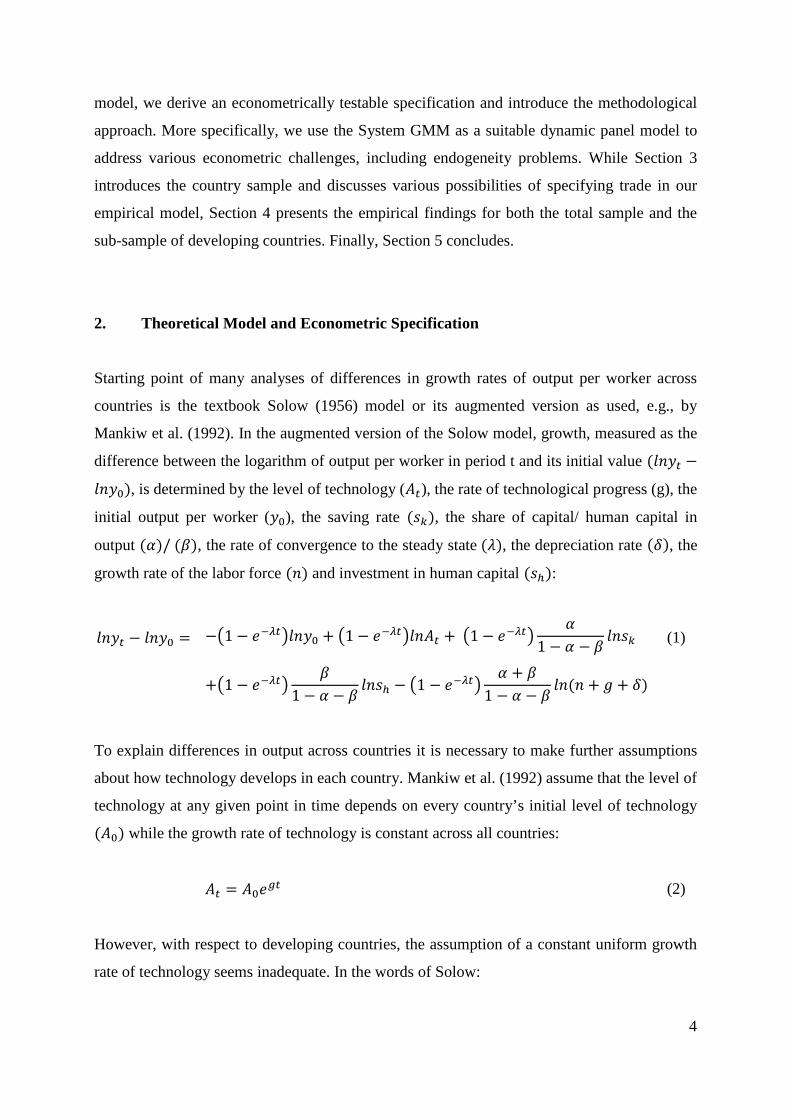
Starting point of many analyses of differences in growth rates of output per worker across

countries is the textbook Solow (1956) model or its augmented version as used, e.g., by

Mankiw et al. (1992). In the augmented version of the Solow model, growth, measured as the

difference between the logarithm of output per worker in period t and its initial value (���� −

����), is determined by the level of technology (�), the rate of technological progress (g), the

initial output per worker (��), the saving rate (�), the share of capital/ human capital in

output (�)/(�), the rate of convergence to the steady state(�), the depreciation rate (�), the

growth rate of the labor force (�) and investment in human capital (�):

���� − ���� = −�1 − ��������� + �1 − �������� +�1 − ������

1 − � − ���� (1)

+�1 − �����

�1 − � − �

��� − �1 − ������ + �

1 − � − ���(� + � + �)

To explain differences in output across countries it is necessary to make further assumptions

about how technology develops in each country. Mankiw et al. (1992) assume that the level of

technology at any given point in time depends on every country’s initial level of technology

(�) while the growth rate of technology is constant across all countries:

� = ���� (2)

However, with respect to developing countries, the assumption of a constant uniform growth

rate of technology seems inadequate. In the words of Solow:

5

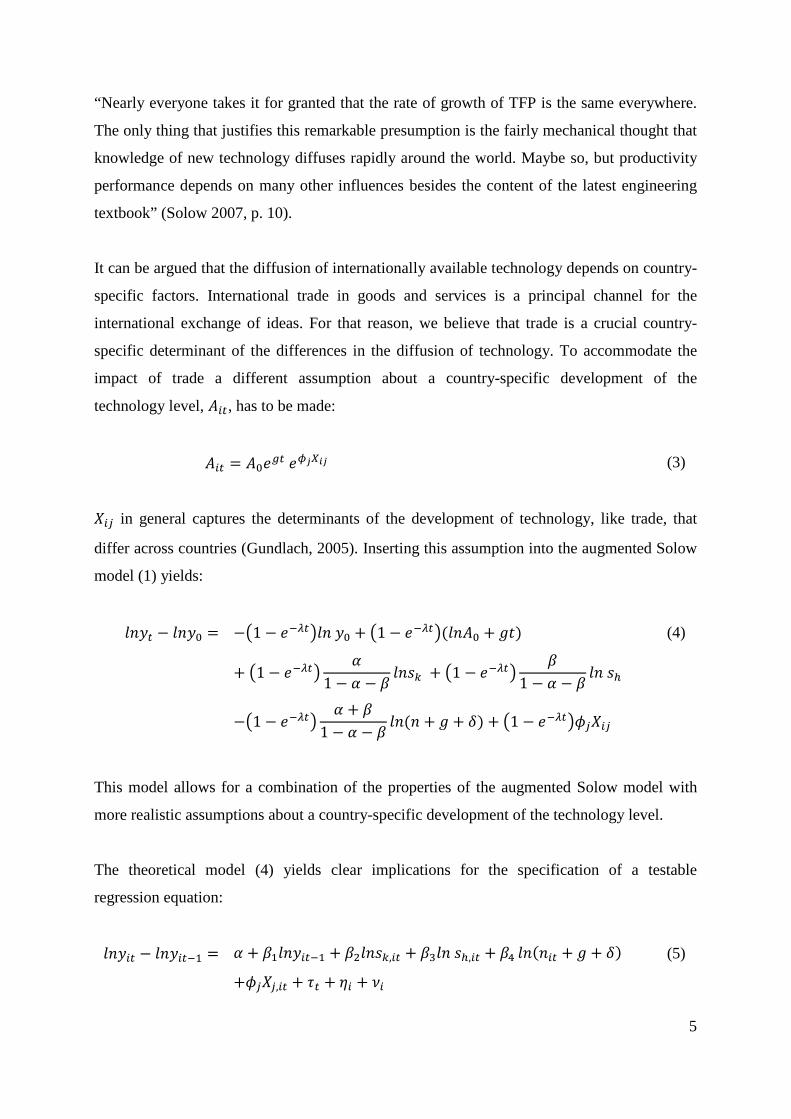
“Nearly everyone takes it for granted that the rate of growth of TFP is the same everywhere.

The only thing that justifies this remarkable presumption is the fairly mechanical thought that

knowledge of new technology diffuses rapidly around the world. Maybe so, but productivity

performance depends on many other influences besides the content of the latest engineering

textbook” (Solow 2007, p. 10).

It can be argued that the diffusion of internationally available technology depends on country-

specific factors. International trade in goods and services is a principal channel for the

international exchange of ideas. For that reason, we believe that trade is a crucial country-

specific determinant of the differences in the diffusion of technology. To accommodate the

impact of trade a different assumption about a country-specific development of the

technology level, ��, has to be made:

�� = ������� !� (3)

"�# in general captures the determinants of the development of technology, like trade, that

differ across countries (Gundlach, 2005). Inserting this assumption into the augmented Solow

model (1) yields:

���� − ���� = −�1 − ��������� + �1 − �����(��� + �$) (4)

+�1 − �����

�1 − � − �

��� + �1 − ������

1 − � − ����

−�1 − �����

� + �1 − � − �

��(� + � + �) + �1 − �����%#"�#

This model allows for a combination of the properties of the augmented Solow model with

more realistic assumptions about a country-specific development of the technology level.

The theoretical model (4) yields clear implications for the specification of a testable

regression equation:

����� − ������& = � + �&������& + �'���,�� + �)���,�� + �* ��(��� + � + �) (5)

+%#"#,�� + +� + ,� + -�

6

or equivalently:

����� = � + (�& + 1)������& + �'���,�� + �) �� �,�� + �* ��(��� + � + �) (6)

+%#"#,�� + +� + ,� + -�

The model includes period-specific intercepts (+�), accounting for period-specific effects like

changes in productivity affecting all countries, country-specific fixed-effects (,�) and an

independent and identically distributed error term (-�).

Estimating the above model, however, is plagued by some well-known difficulties. The

explanatory variables are potentially endogenous and measured with error. Some important

variables, e.g., the initial level of technology and other country-specific effects, are not

observable and omitted in the estimation. Estimating this dynamic panel data model by

ordinary least squares (OLS) or within group estimations will potentially lead to biased

results. To solve this problem, we have to follow an instrumental variable approach, that is, to

find adequate instruments that are correlated with the endogenous explanatory variable but are

not correlated with our dependent variable. As it is difficult to think of appropriate external

instruments, Bond et al. (2001) recommend the System GMM estimator suggested by

Arellano and Bover (1995) and Blundell and Bond (1998) to solve the difficulties of empirical

growth regressions. The System GMM estimator does not require any external instruments

but uses lagged levels and differences between two periods as instruments for current values

of the endogenous explanatory variables. The procedure simultaneously estimates a system of

equations that consists of both first-differences as well as levels of the estimation equation.

Taking first differences eliminates country-specific fixed-effects and solves the problem of

the potential omission of the initial level of technology and other time invariant country-

specific factors influencing growth. This approach ensures that we can concentrate on the

impact of the explanatory variables on income per capita growth and not vice versa.

7

3. Data and Sample

The panel dataset used in this study consists of up to 108 countries (of which 87 are

developing countries) covering the period 1971-2005 (1970-2005 for the GDP per capita

variable).6 Unfortunately, data is not available for all countries for the first periods resulting in

a slightly unbalanced panel. To reduce the impact of business cycles we use a total of seven

five-year averages for all variables, 1971-1975, 1976-1980 and so on, until 2005. As

dependent variable, we use the growth rates of income calculated as the difference in the

logarithm of GDP per capita (in constant 2000 US dollars) between the last year of the

previous period and the last year of the period under consideration (the variable is labeled as

∆GDPpc).7

In our model, we include the control variables of the core Solow model following the

specification of Mankiw et al. (1992). The saving rate (�) is approximated by the investment

share of real GDP per capita in current prices (InvestmentShare). For the growth rate of the

labor force (n), we use the average population growth rate which is the difference between the

logarithm of total population at the beginning and the end of the period. As in Mankiw et al.

(1992), the growth rate of the world technology frontier (g) and the depreciation rate (�) are

assumed to be constant across countries. The term ln(� + � + �) is calculated as the

logarithm of the population growth rate and 0.05 p.a. (� + �) as a constant

(PopulationGrowth). Investment in human capital (�) is approximated by educational

attainment, more precisely the average years of secondary schooling in the total population

over age 15 (Education). Finally, we include the initial level of GDP per capita

(GDPpc (t-1)).

There is no unique indication in which manner trade should enter growth estimations. A

commonly used measure in the analyses of the relationship between trade and growth is total

trade volume (of both goods and services) as a share of total GDP (TradeShare). The trade-to-

GDP ratio is often referred to as the “trade openness ratio”. The term does not necessarily

6 See Appendix A for data sources and Appendix D for a list of countries included. Descriptive statistics can be found in Appendix B and C. 7 The results are not sensitive to alternatively using the difference between the first and the last year of the current period. The Solow model suggests using GDP per worker instead of GDP per capita which might be important if dependency ratios vary across countries. Mankiw et al. (1992) use per worker data while other authors, e.g., Caselli et al. (1996) and Islam (1995), use per capita data. Hoeffler (2002) has found that results are not sensitive to either choice.

8

imply low tariffs or low non-tariff barriers but simply measures how much of a country’s

GDP is traded. In a dynamic panel setting, we argue that the trade-to-GDP ratio is not suitable

to measure correlation or causality between trade and growth. If trade in general has a positive

impact on growth in the sense that increasing trade (volumes) does increase GDP through the

channels described above, the “trade openness ratio” fails to adequately capture this effect

over time. Depending on the elasticity of trade on GDP, increasing the trade volume might

increase GDP in a proportionately larger, smaller or exactly equal way. Consequently, the

“trade openness ratio” can either increase, decrease or stay the same due to an increase in

trade and its corresponding changes in GDP. A positive impact of trade on GDP can lead to a

decrease in the “trade openness ratio” as an increase of the numerator might be offset by a

larger increase of the denominator.

We propose a solution to that problem by using lagged values of total GDP for the “trade

openness ratio” instead of trade volume and GDP of the same period. Using lagged values has

the same effect of normalizing trade volumes across countries but that ratio does not suffer

from biases due to simultaneous changes in both variables. TradeShare (GDP t-1) is

calculated as exports and imports of goods and services in current US$ divided by total GDP

in current US$ lagged by one period.

Furthermore, we use the logarithm of total trade volume (Trade). This variable follows the

assumption that, abstracting from the actual size of a country, trading more may be associated

with having access to a larger pool of technology. Focusing on the growth rate of total trade

volume (TradeGrowth) assumes that it is especially the expansion of trade and its associated

access to supplementary technologies that boosts growth. Another approach for relating trade

to the size of a country is to divide trade by total population yielding a measure of trade per

capita (TradePop). The intuition of that variable is not apparent straight away. In contrast to

physical capital and labor that enter the production function in per capita terms, advances in

technology can be implemented simultaneously by several individuals.

In general, System GMM estimation results are quite sensitive with respect to the treatment of

right hand side variables as predetermined, endogenous or strictly exogenous. In our model

the only variables that are strictly exogenous are the year dummies. Theory serves as a

guideline for classifying the remaining variables. The lagged GDP per capita and the

9

education variable can be treated as predetermined.8 Lagging these variables by at least one

period yields valid instruments for the equation in differences and correspondingly their first

differences valid instruments for the equation in levels. The investment rate as a share of

GDP, the population growth rate and all different trade variables are treated as endogenous

since contemporary shocks are likely to affect both GDP per capita growth rates as well as

those explanatory variables. To obtain valid instruments for the endogenous explanatory

variables, observations lagged by at least two periods are used.

4. Empirical Results

Following the model specification and the introduction of the variables, we now turn to the

empirical results. As a benchmark, we first focus on the augmented Solow model that

explains differences in GDP per capita growth across countries and time with the initial level

of GDP per capita, the investment rate, population growth and human capital. The first three

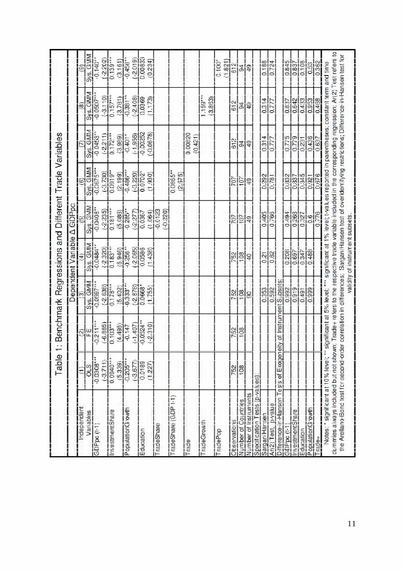
columns of Table 1 present the estimation results of the augmented Solow model obtained by

using different estimation techniques: OLS (column 1), fixed-effects estimation (column 2)

and System GMM (columns 3 and 4). In dynamic panel data models, due to potentially

endogenous estimators the results of the OLS estimation may be biased upwards while the

results of the fixed-effects estimation may be biased downwards. The System GMM results

should be somewhere in between both biased results. The OLS estimation (column 1) yields a

relatively high coefficient of the initial level of GDP per capita while for the fixed-effects

estimation (column 2) the coefficient has considerably decreased in magnitude. The

coefficient of the initial level of GDP per capita obtained by the System GMM estimation

(column 3) lies comfortably between both albeit closer to the OLS results. For the System

GMM regression, all other variables of the augmented Solow model have the expected sign.

The investment rate as a share of GDP (InvestmentShare) has a positive and highly significant

coefficient. Increases in population growth (PopulationGrowth) have a significantly negative

effect on GDP per capita growth rates and the influence of investment in human capital

(Education) is positive and significant at the conventional 10 per cent level.

8 Education data is collected every 5 years by Barro and Lee (2010). We include the educational attainment at the start of each period, e.g., the observation of 1970 for the period 1971-1975 in the estimation equation and subsequently treat that variable as predetermined. This has been done in a similar form by Hoeffler (2002). A different possibility would be to take the average of two consequent observations and treat the education variable as either predetermined or endogenous. Our results are not sensitive to either choice.

10

The Sargan/Hansen test of overidentifying restrictions confirms the joint validity of our

instruments. The p-value of the Arellano-Bond test for second-order correlation in differences

(Ar(2) Test) rejects first-order serial correlation in levels. The difference-in-Hansen tests

confirm for all variables the individual validity of the instruments. In the System GMM

regression of column 3, all realizations of the potentially endogenous explanatory variables

lagged by two periods and more have been included as instruments. In the case of the

education variable, the realization lagged by one period serves as an additional valid

instrument. As we use lagged levels and lagged differences, the number of instruments can be

quite large. Yet too many instruments can overfit the model and also weaken the power of the

Sargan/ Hansen test.9 Thus, we reduce the size of the instrument matrix by restricting the

number of lags used. In the next step, we therefore replicate the estimation reducing the

number of instruments. In column 4 only the first available instrument has been employed.

Changing the lag-structure does not fundamentally alter our results. Only the coefficient of

the Education variable drops slightly below the 10 per cent level of confidence. All test

statistics confirm the validity of instruments for the reduced lags. Both our System GMM

regressions (column 3 and 4) are very much in line with other applications of that estimation

technique to test the augmented Solow model.10

9 In columns 1-3 the total number of instruments is below the number of countries. However, the extensive lag-structure limits the possibility of adding further endogenous explanatory variables that require additional instruments and easily increases their number to a critical amount. 10 We are able to replicate the basic findings of previous works, e.g., Bond et al. (2001) and Hoeffler (2002).

11

12

Having established a valid benchmark, we subsequently include our main variable of interest:

trade. The first candidate is the widely used TradeShare variable (column 5), which is the

total trade volume divided by total GDP of the same period. Including that additional variable

does not fundamentally alter the results of the benchmark regression but the coefficient of the

trade variable is negative and not significant. As argued above, we do not believe that this

TradeShare variable adequately captures the impact of trade on GDP per capita growth.

Including our preferred measure of that influence, TradeShare (GDP t-1), fundamentally

changes the regression results for the impact of trade on GDP per capita growth (column 6).

TradeShare (GDP t-1) has a positive coefficient and is significant at the 5 per cent level of

confidence. At the same time, the control variables of the augmented Solow model maintain

their expected influence and all test statistics confirm the validity of our instruments. An

increase in the volume of exports and imports divided by total GDP of the previous period,

TradeShare (GDP t-1), by one unit at the mean (106.0) is associated with an increase in GDP

per capita growth of 0.08 percentage points over a period of five years. For an interpretation

of the economic significance, it has to be taken into account that the TradeShare (GDP t-1)

variable varies considerably across countries or over time. Using our alternative trade share

variable in combination with the valid instrumentation of the System GMM estimator allows

us to establish a causal relation between trade and differences in GDP per capita growth.

Trade does have a positive impact on GDP per capita growth and our results show that it

indeed matters in which way trade enters empirical growth regressions.

TradeShare (GDP t-1) is our preferred measure of the impact of trade on GDP per capita

growth, but we also run regressions with different variations of the trade variable to be able to

compare the results. For the logarithm of total trade volume, Trade, no significant results can

be found (column 7). The average growth rate of trade, TradeGrowth, has a positive and

highly significant effect (column 8). An increase in TradeGrowth by one unit increases GDP

per capita growth by 1.16 percentage points (over 5 years). Including trade divided by a

country’s total population, TradePop, (column 9) yields a positive and significant effect as

well. The marginal effect at the mean of a one unit increase of TradePop (4565.26 US$) is an

increase in GDP per capita growth of 0.002 percentage points over a period of five years.

Employing alternative trade measures confirms the significant influence of trade on GDP per

capita growth.

13

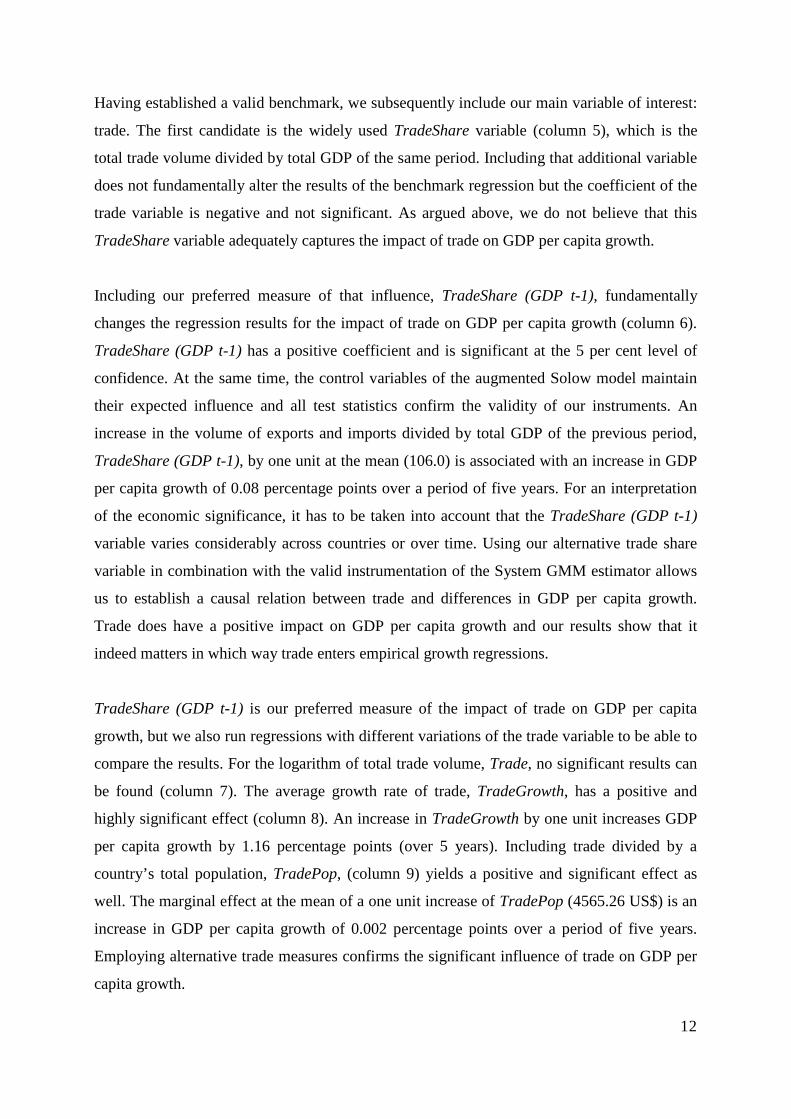
Next, we examine whether both channels of how trade influences GDP per capita growth –

via the absolute volume of trade (or alternatively the volume divided by total GDP or

population) and its growth rate – can be substantiated even if they occur simultaneously.

Table 2 shows the regression results where we include both the TradeGrowth variable and

one of our additional trade measures in the analysis. First of all, we focus on the conventional

TradeShare variable (column 1). While the growth rate of trade, TradeGrowth, has a positive

and highly significant effect, the additional TradeShare variable is not significant, reflecting

14

our results from Table 1. When we include our novel TradeShare (GDP t-1) variable, both

TradeGrowth and TradeShare (GDP t-1) have a positive and highly significant effect (column

2). In column 3 TradeGrowth and Trade are included. The results confirm the importance of

TradeGrowth while no evidence can be found for the logarithm of total trade volume.11

Finally, in column 4 both TradeGrowth and TradePop are included which yields significant

results for both variables. The results of Table 2 once more confirm the adequateness and

robustness of our TradeShare (GDP t-1) variable. In addition, we show that both channels,

trade and the expansion of trade, have an independent impact on GDP per capita growth.

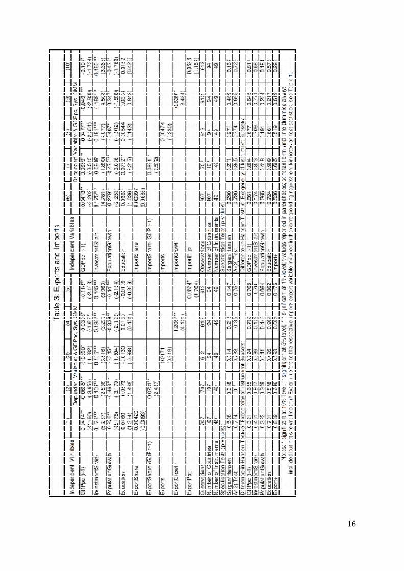
It is obvious to ask if our results for total trade hold true for imports and exports

independently as well. Table 3 repeats the exercise we have done for total trade for its two

components, showing a similar picture: ExportShare (column 1) with the current realization

of total GDP as its denominator is not significant. Employing the 5 year lagged realization of

total GDP, ExportShare (GDP t-1), yields positive and significant results for the export

measure (column 2). The coefficient of the logarithm of total export volume, Exports,

(column 3) is not significant while the average growth rate of exports, ExportGrowth,

(column 4) and ExportPop, (column 5) are again positive and significant. The results for the

import variables (columns 6-10) are qualitatively almost the same as for the export variables

with the exception of ImportPop (column 10).12

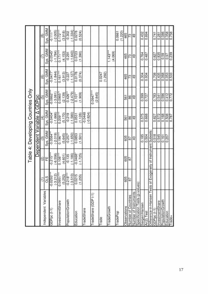
The evidence established so far has been for the total sample, including both developed and

developing countries. The question arises if the positive influence of trade on income growth

is robust for a sample of developing countries only. It might be argued that for the developing

countries the preconditions for the realization of a positive trade-income-growth nexus are not

in place yet. Table 4 sheds some light on this issue by showing the results for a subsample of

developing countries.13 Columns 1-3 set up the benchmark repeating the exercise of

comparing the regression results obtained by the System GMM estimator with those of the

OLS and fixed-effects estimation. As expected, the System GMM coefficient (column 3) for

11 In this regression, however, the test statistics of the Difference-in-Hansen test cast doubt on the validity of our instruments for the total trade volume variable. 12 Both imports and exports are highly correlated (with a correlation coefficient of 0.85 for the observations included in our sample). 13 All countries included are listed in Appendix D. In order to avoid a sample selection bias we focus on countries that have been considered developing countries in 1970.The World Bank classification of countries as low or middle income countries which are commonly considered as developing countries started in 1987 only. We include all of those countries that were classified as low or middle income countries in that year (World Bank 2011).

15

the initial level of per capita GDP lies size wise between the OLS (column 1) and fixed-

effects estimation results (column 2). The control variables have the expected influence and

the test statistics confirm the validity of the instruments obtained by including the twice

lagged observation for all endogenous explanatory variables and the once lagged observation

for the Education variable.

Starting from a valid benchmark, we add the TradeShare variable (column 4) and again do

not find significant results for that measure of trade. Including the measure TradeShare (GDP

t-1) (column 5) confirms the positive and significant effect of trade on GDP per capita growth

for developing countries. An increase in the volume of exports and imports divided by total

GDP of the previous period, TradeShare (GDP t-1), by one unit at the developing countries’

mean (99.96) is associated with an increase in GDP per capita growth of 0.09 percentage

points over a period of five years. For TradeGrowth (column 7), the positive and significant

impact is confirmed as well. An increase in TradeGrowth by one unit increases GDP per

capita growth by 1.14 percentage points. For Trade (column 7) and TradePop (column 8), the

coefficients do not reach conventional significance level. The results show that the positive

effect of both trade and the expansion of trade can be found for developing countries as well.

16

17

18

5. Conclusion

An increased integration of countries into the world economy through trade is seen as a

fundamental cause of differences in income and growth across countries. The aim of this

paper is to establish a causal linkage between trade and GDP per capita growth. To reach that

aim several specifications of trade in empirical growth estimations are discussed. In a

dynamic panel setting, it is argued that the often used trade-to-GDP or “trade openness” ratio,

which is the volume of exports and imports as a share of total GDP does not adequately

capture the impact of trade on GDP per capita growth. Assuming a causal linkage between

trade and income, changes in trade (volume) over time would always cause corresponding

changes in income. This dynamic effect is not accounted for by the “trade openness ratio”.

Due to changes in the numerator, trade volume, and the associated changes in the

denominator, GDP, the “trade openness ratio” can either increase, decrease or stay the same.

Building on these considerations, a different trade variable is preferred: the volume of exports

and imports as a share of lagged total GDP. This trade measure avoids a potential bias when

both volume of exports and imports and total GDP change simultaneously.

Using the alternative trade measure in combination with the valid instrumentation of the

System GMM estimator allows establishing a causal relation between trade and differences in

GDP per capita growth. Trade does indeed have a positive and significant impact on growth.

We find evidence that the expansion of trade, e.g., through its associated access to additional

technologies, has a significant impact on income growth as well. In addition, it can be shown

that both channels, trade and the expansion of trade, have an independent influence on GDP

per capita growth. The same results hold true for both exports and imports separately.

The positive influence of trade on income growth is also confirmed for a sample of

developing countries only. Trade has been found to be effective in fostering economic growth

in developing countries. These findings are crucial for the current discourse in the

“development community” as they underpin the importance of trade related development aid,

for example, the Aid for Trade initiative.

19

References

Arellano, M. and O. Bover (1995), Another Look at the Instrumental Variable Estimation of

Error-components Models, Journal of Econometrics 68(1): 29-51.

Barro, R. and J.-W. Lee (2010), A New Data Set of Educational Attainment in the World,

1950-2010, NBER Working Papers 15902.

Barro, R. and X. Sala-i-Martin (1997), Technological Diffusion, Convergence, and Growth,

Journal of Economic Growth 2(1): 1-26.

Ben-David, D. (1993), Equalizing Exchange: Trade Liberalization and Income Convergence,

Quarterly Journal of Economics 108(3): 653-79.

Bernard, A. B. and J. B. Jensen (2004), Why Some Firms Export, Review of Economics and

Statistics 86(2): 561-569.

Bernard, A. B.; J. Eaton; J. B. Jensen and S. Kortum (2003), Plants and Productivity in

International Trade, American Economic Review 93(4): 1268-1290.

Blundell, R. and S. Bond (1998), Initial Conditions and Moment Restrictions in Dynamic

Panel Data Models, Journal of Econometrics 87(1): 115-143.

Bond, S.; A. Hoeffler and J. Temple (2001), GMM Estimation of Empirical Growth Models,

CEPR Discussion Papers 3048.

Caselli, F.; G. Esquivel and F. Lefort (1996), Reopening the Convergence Debate: A New

Look at Cross-Country Growth Empirics, Journal of Economic Growth 1(3): 363-89.

Dollar, D. and A. Kraay (2004), Trade, Growth, and Poverty, Economic Journal 114(493):

F22-F49.

Dollar, D. (1992), Outward-Oriented Developing Economies Really Do Grow More Rapidly:

Evidence from 95 LDCs, 1976-1985, Economic Development and Cultural Change

40(3): 523-44.

Edwards, S. (1998), Openness, Productivity and Growth: What Do We Really Know?,

Economic Journal 108(447): 383-98.

Feyrer J. (2009), Trade and Income - Exploiting Time Series in Geography, NBER Working

Papers 14910.

20

Frankel, J. and D. Romer (1999), Does Trade Cause Growth?, American Economic Review

89(3): 379-399.

Grossman, G. and E. Helpman (1991), Innovation and Growth in the Global Economy,

Cambridge, MA: MIT Press.

Gundlach, E. (2005), Solow vs. Solow: Notes on Identification and Interpretation in the

Empirics of Growth and Development, Review of World Economics

(Weltwirtschaftliches Archiv) 141(3): 541-556.

Heston, A.; R. Summers and B. Aten (2010), Penn World Table, Center for International

Comparisons of Production, Income and Prices at the University of Pennsylvania.

Hoeffler, A. (2002), The Augmented Solow Model and the African Growth Debate, Oxford

Bulletin of Economics and Statistics 64(2): 135-58.

Islam, N. (1995), Growth Empirics: A Panel Data Approach, Quarterly Journal of Economics

110(4): 1127-70.

Krugman, P. (1979), A Model of Innovation, Technology Transfer, and the World

Distribution of Income, Journal of Political Economy 87(2): 253-66.

Lee, J.-W. (1993), International Trade, Distortions, and Long-Run Economic Growth, IMF

Staff Papers 40(2): 299-328.

Mankiw, N. G.; D. Romer and D. N. Weil (1992), A Contribution to the Empirics of

Economic Growth, Quarterly Journal of Economics 107(2): 407-437.

Manole, V. and M. Spatareanu (2010), Trade Openness and Income – A Re-examination,

Economics Letters 106(1): 1-3.

Noguer, M. and M. Siscart (2005), Trade Raises Income, a Precise and Robust Result,

Journal of International Economics 65(2): 447-460.

Obstfeld, M. and A. M. Taylor (2003), Globalization and Capital Markets, NBER Chapters:

Globalization in Historical Perspective, 121-188, NBER.

Rivera-Batiz, L. A. and P. M. Romer (1991), Economic Integration and Endogenous Growth,

Quarterly Journal of Economics 106(2): 531-55.

Rodríguez, F. R. (2007), Openness and growth: What Have We Learned?, DESA Working

Papers 51, New York: United Nations, Department of Economics and Social Affairs.

21

Rodríguez, F. R. and D. Rodrik (2001), Trade Policy and Economic Growth: A Skeptic's

Guide to the Cross-National Evidence, NBER Macroeconomics Annual 2000, 15: 261-

338.

Sachs, J. D. and A. Warner (1995), Economic Reform and the Process of Global Integration,

Brookings Papers on Economic Activity 26(1): 1-118.

Sala-i-Martin, X.; G. Doppelhofer and R. I. Miller (2004), Determinants of Long-term

Growth: A Bayesian Averaging of Classical Estimates (BACE) Approach, American

Economic Review 94(4): 813-835.

Solow, R. M. (2007), The Last 50 Years in Growth Theory and the Next 10, Oxford Review of

Economic Policy 23(1): 3-14.

Solow, R. M. (1956), A Contribution to the Theory of Economic Growth, Quarterly Journal

of Economics 70(1): 65-94.

Squalli, J. and K. Wilson (2011), A New Measure of Trade Openness, World Economy

34(10): 1745-1770.

Vernon, R. (1966), International Investment and International Trade in the Product Cycle,

Quarterly Journal of Economics 80(2): 190-207.

Wacziarg, R. and K. H. Welch (2008), Trade Liberalization and Growth: New Evidence,

World Bank Economic Review 22(2): 187-231.

Warner, A. (2003), Once More into the Breach: Economic Growth and Integration, Center for

Global Development Working Papers 34.

World Bank (2010), World Development Indicators, Washington, D.C.: World Bank.

Yanikkaya, H. (2003), Trade Openness and Economic Growth: A Cross-country Empirical

Investigation, Journal of Development Economics 72(1): 57-89.

Young, A. (1991), Learning by Doing and the Dynamic Effects of International Trade,

Quarterly Journal of Economics 106(2): 369-405.

22

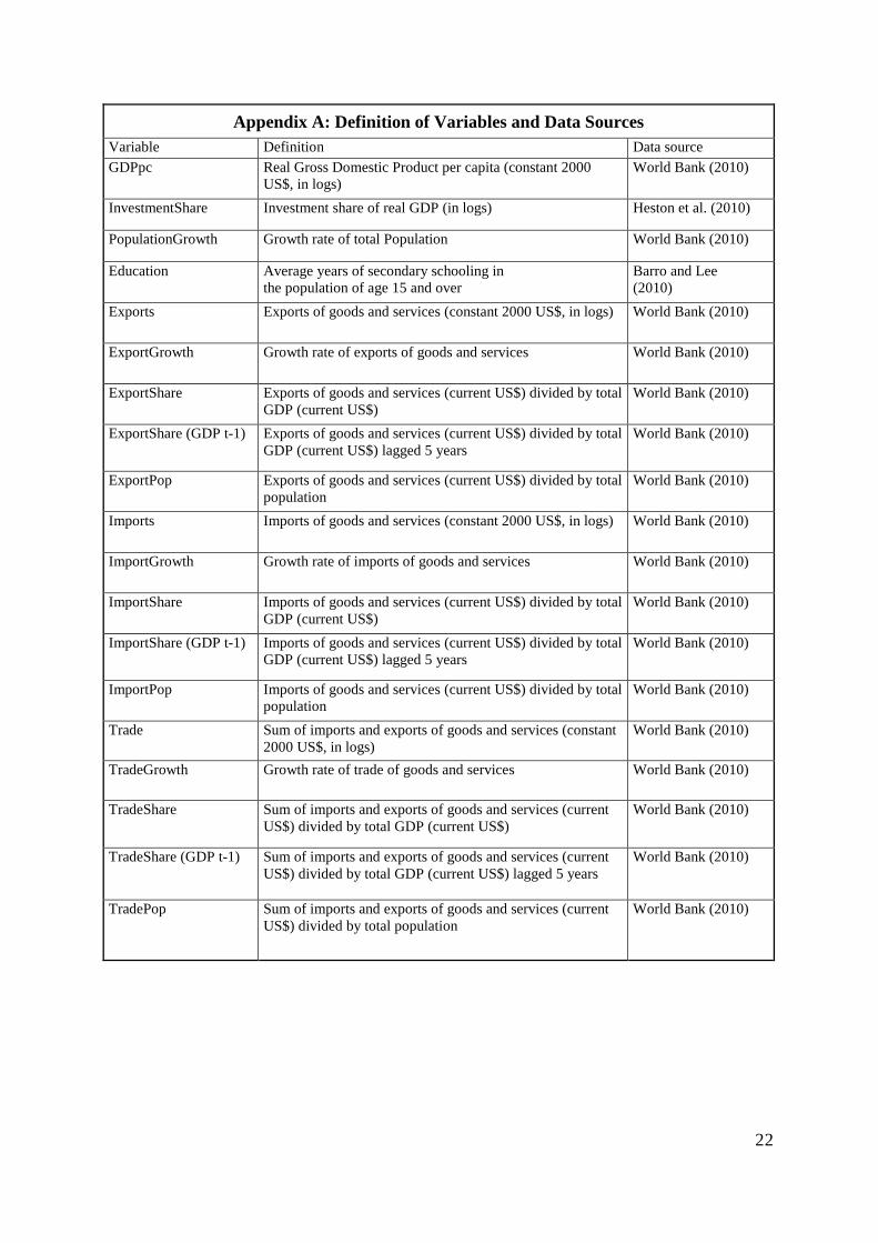
Appendix A: Definition of Variables and Data Sources Variable Definition Data source GDPpc Real Gross Domestic Product per capita (constant 2000

US$, in logs) World Bank (2010)

InvestmentShare Investment share of real GDP (in logs) Heston et al. (2010)

PopulationGrowth Growth rate of total Population World Bank (2010)

Education Average years of secondary schooling in the population of age 15 and over

Barro and Lee (2010)

Exports Exports of goods and services (constant 2000 US$, in logs) World Bank (2010)

ExportGrowth Growth rate of exports of goods and services World Bank (2010)

ExportShare Exports of goods and services (current US$) divided by total GDP (current US$)

World Bank (2010)

ExportShare (GDP t-1) Exports of goods and services (current US$) divided by total GDP (current US$) lagged 5 years

World Bank (2010)

ExportPop Exports of goods and services (current US$) divided by total population

World Bank (2010)

Imports Imports of goods and services (constant 2000 US$, in logs) World Bank (2010)

ImportGrowth Growth rate of imports of goods and services World Bank (2010)

ImportShare Imports of goods and services (current US$) divided by total GDP (current US$)

World Bank (2010)

ImportShare (GDP t-1) Imports of goods and services (current US$) divided by total GDP (current US$) lagged 5 years

World Bank (2010)

ImportPop Imports of goods and services (current US$) divided by total population

World Bank (2010)

Trade Sum of imports and exports of goods and services (constant 2000 US$, in logs)

World Bank (2010)

TradeGrowth Growth rate of trade of goods and services World Bank (2010)

TradeShare Sum of imports and exports of goods and services (current US$) divided by total GDP (current US$)

World Bank (2010)

TradeShare (GDP t-1) Sum of imports and exports of goods and services (current US$) divided by total GDP (current US$) lagged 5 years

World Bank (2010)

TradePop Sum of imports and exports of goods and services (current US$) divided by total population

World Bank (2010)

23

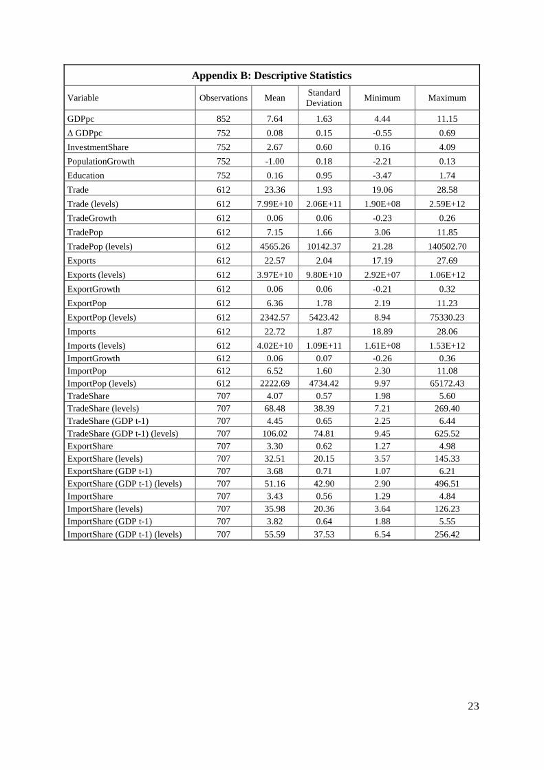
Appendix B: Descriptive Statistics

Variable Observations Mean Standard Deviation

Minimum Maximum

GDPpc 852 7.64 1.63 4.44 11.15

∆ GDPpc 752 0.08 0.15 -0.55 0.69

InvestmentShare 752 2.67 0.60 0.16 4.09

PopulationGrowth 752 -1.00 0.18 -2.21 0.13

Education 752 0.16 0.95 -3.47 1.74

Trade 612 23.36 1.93 19.06 28.58

Trade (levels) 612 7.99E+10 2.06E+11 1.90E+08 2.59E+12

TradeGrowth 612 0.06 0.06 -0.23 0.26

TradePop 612 7.15 1.66 3.06 11.85

TradePop (levels) 612 4565.26 10142.37 21.28 140502.70

Exports 612 22.57 2.04 17.19 27.69

Exports (levels) 612 3.97E+10 9.80E+10 2.92E+07 1.06E+12

ExportGrowth 612 0.06 0.06 -0.21 0.32

ExportPop 612 6.36 1.78 2.19 11.23

ExportPop (levels) 612 2342.57 5423.42 8.94 75330.23

Imports 612 22.72 1.87 18.89 28.06

Imports (levels) 612 4.02E+10 1.09E+11 1.61E+08 1.53E+12 ImportGrowth 612 0.06 0.07 -0.26 0.36 ImportPop 612 6.52 1.60 2.30 11.08 ImportPop (levels) 612 2222.69 4734.42 9.97 65172.43 TradeShare 707 4.07 0.57 1.98 5.60 TradeShare (levels) 707 68.48 38.39 7.21 269.40 TradeShare (GDP t-1) 707 4.45 0.65 2.25 6.44 TradeShare (GDP t-1) (levels) 707 106.02 74.81 9.45 625.52 ExportShare 707 3.30 0.62 1.27 4.98 ExportShare (levels) 707 32.51 20.15 3.57 145.33 ExportShare (GDP t-1) 707 3.68 0.71 1.07 6.21 ExportShare (GDP t-1) (levels) 707 51.16 42.90 2.90 496.51 ImportShare 707 3.43 0.56 1.29 4.84 ImportShare (levels) 707 35.98 20.36 3.64 126.23 ImportShare (GDP t-1) 707 3.82 0.64 1.88 5.55

ImportShare (GDP t-1) (levels) 707 55.59 37.53 6.54 256.42

24

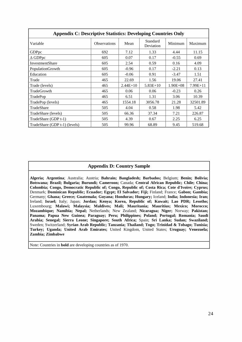
Appendix C: Descriptive Statistics: Developing Countries Only

Variable Observations Mean Standard Deviation

Minimum Maximum

GDPpc 692 7.12 1.33 4.44 11.15 ∆ GDPpc 605 0.07 0.17 -0.55 0.69 InvestmentShare 605 2.54 0.59 0.16 4.09 PopulationGrowth 605 -0.96 0.17 -2.21 0.13 Education 605 -0.06 0.91 -3.47 1.51 Trade 465 22.69 1.56 19.06 27.41 Trade (levels) 465 2.44E+10 5.83E+10 1.90E+08 7.99E+11 TradeGrowth 465 0.06 0.06 -0.23 0.26 TradePop 465 6.51 1.31 3.06 10.39 TradePop (levels) 465 1554.18 3056.78 21.28 32501.89 TradeShare 505 4.04 0.58 1.98 5.42 TradeShare (levels) 505 66.36 37.34 7.21 226.87 TradeShare (GDP t-1) 505 4.39 0.67 2.25 6.25

TradeShare (GDP t-1) (levels) 505 99.96 68.89 9.45 519.68

Appendix D: Country Sample

Algeria; Argentina ; Australia; Austria; Bahrain; Bangladesh; Barbados; Belgium; Benin; Bolivia; Botswana; Brazil; Bulgaria; Burundi; Cameroon; Canada; Central African Republic; Chile; China; Colombia; Congo, Democratic Republic of; Congo, Republic of; Costa Rica; Cote d'Ivoire; Cyprus; Denmark; Dominican Republic; Ecuador; Egypt; El Salvador; Fiji; Finland; France; Gabon; Gambia; Germany; Ghana; Greece; Guatemala; Guyana; Honduras; Hungary; Iceland; India; Indonesia; Iran; Ireland; Israel; Italy; Japan; Jordan; Kenya; Korea, Republic of; Kuwait; Lao PDR; Lesotho; Luxembourg; Malawi; Malaysia; Maldives; Mali; Mauritania; Mauritius; Mexico; Morocco; Mozambique; Namibia; Nepal; Netherlands; New Zealand; Nicaragua; Niger; Norway; Pakistan; Panama; Papua New Guinea; Paraguay; Peru; Philippines; Poland; Portugal; Romania; Saudi Arabia; Senegal; Sierra Leone; Singapore; South Africa; Spain; Sri Lanka; Sudan; Swaziland; Sweden; Switzerland; Syrian Arab Republic; Tanzania; Thailand; Togo; Trinidad & Tobago; Tunisia; Turkey; Uganda; United Arab Emirates; United Kingdom, United States; Uruguay; Venezuela; Zambia; Zimbabwe

Note: Countries in bold are developing countries as of 1970.

HWWI Research Papersseit 2011

122 Immigration and Election Outcomes − Evidence from City Districts in Hamburg

Alkis Henri Otto, Max Friedrich Steinhardt, April 2012

121 Renewables in the energy transition − Evidence on solar home systems and

lighting fuel choice in Kenya

Jann Lay, Janosch Ondraczek, Jana Stöver, April 2012

119 Creative professionals and high-skilled agents: Polarization of employment

growth?

Jan Wedemeier, March 2012

118 Unraveling the complexity of U.S. presidential approval. A multi-dimensional

semi-parametric approach

Michael Berlemann, Soeren Enkelmann, Torben Kuhlenkasper, February 2012

117 Policy Options for Climate Policy in the Residential Building Sector: The Case of

Germany

Sebastian Schröer, February 2012

116 Fathers’ Childcare: the Difference between Participation and Amount of Time

Nora Reich, February 2012

115 Fathers’ Childcare and Parental Leave Policies − Evidence from Western

European Countries and Canada

Nora Reich, Christina Boll, Julian Leppin, Hamburg, February 2012

114 What Drives FDI from Non-traditional Sources? A Comparative Analysis of the

Determinants of Bilateral FDI Flows

Maximiliano Sosa Andrés, Peter Nunnenkamp, Matthias Busse,

Hamburg, January 2012

113 On the predictive content of nonlinear transformations of lagged

autoregression residuals and time series observations

Anja Rossen, Hamburg, October 2011

112 Regional labor demand and national labor market institutions in the EU15

Helmut Herwartz, Annekatrin Niebuhr, Hamburg, October 2011

111 Unemployment Duration in Germany – A comprehensive study with dynamic

hazard models and P-Splines

Torben Kuhlenkasper, Max Friedrich Steinhardt, Hamburg, September 2011

110 Age, Life-satisfaction, and Relative Income

Felix FitzRoy, Michael Nolan, Max Friedrich Steinhardt, Hamburg, July 2011

109 The conjoint quest for a liberal positive program: “Old Chicago”, Freiburg and

Hayek

Ekkehard Köhler, Stefan Kolev, Hamburg, July 2011

108 Agglomeration, Congestion, and Regional Unemployment Disparities

Ulrich Zierahn, Hamburg, July 2011

107 Efficient Redistribution: Comparing Basic Income with Unemployment Benefit

Felix FitzRoy, Jim Jin, Hamburg, March 2011

106 The Resource Curse Revisited: Governance and Natural Resources

Matthias Busse, Steffen Gröning, Hamburg, March 2011

105 Regional Unemployment and New Economic Geography

Ulrich Zierahn, Hamburg, March 2011

104 The Taxation-Growth-Nexus Revisited

K. P. Arin, M. Berlemann, F. Koray, T. Kuhlenkasper, Hamburg, January 2011

The Hamburg Institute of International Economics (HWWI) is an independent economic research institute, based on a non-profit public-private partnership, which was founded in 2005. The University of Hamburg and the Hamburg Chamber of Commerce are shareholders in the Institute .

The HWWI’s main goals are to: • Promote economic sciences in research and teaching;• Conduct high-quality economic research; • Transfer and disseminate economic knowledge to policy makers, stakeholders and the general public.

The HWWI carries out interdisciplinary research activities in the context of the following research areas: • Economic Trends and Global Markets, • Regional Economics and Urban Development, • Sectoral Change: Maritime Industries and Aerospace, • Institutions and Institutional Change, • Energy and Raw Material Markets, • Environment and Climate, • Demography, Migration and Integration, • Labour and Family Economics, • Health and Sports Economics, • Family Owned Business, and• Real Estate and Asset Markets.

Hamburg Institute of International Economics (HWWI)

Heimhuder Str. 71 | 20148 Hamburg | GermanyPhone: +49 (0)40 34 05 76 - 0 | Fax: +49 (0)40 34 05 76 - 776info@hwwi.org | www.hwwi.org