Transmission Pricing 37

7/26/2019 Transmission Pricing 37

http://slidepdf.com/reader/full/transmission-pricing-37 1/15

Transmission pricing using the exact power and lossallocation method for bilateral contracts in a deregulatedelectricity supply industry

Cattareeya Adsoongnoen1, Weerakorn Ongsakul1,*,y, Christoph Maurer2

and Hans-Jurgen Haubrich2

1Energy Field of Study, School of Environment, Resources and Development, Asian Institute of Technology,

Pathumthani 12120, Thailand 2 Institute of Power Systems and Power Economics, RWTH Aachen University, Schinkelstr. 6, 52056 Aachen, Germany

SUMMARY

This paper proposes a new method based on exact power and loss allocation for bilateral transactions under theenhanced single buyer model in the Thai electricity supply industry (Thai ESI). Generally, a transmission network is designed to transfer mainly active power. The transmission pricing for this active power charge in the Thai ESIcomprises three components, namely the transmission use-of-system charge, the connection charge, and thecommon service charge. However, the calculation of transmission pricing, using marginal cost scheme, might notensure revenue requirements of the transmission owner in case of a high reactive power demand in the network because a part of transmission line capacity is subsequently required for the reactive power transfer. Thus, thetriangle method is used to segregate the transmission pricing by classifying active and reactive charges. The usersare charged regarding their system usages by applying the exact power and loss allocation method. The proposedtransmission pricing sends economic incentives to the users with fair charges. It ensures an investment recovery of

the transmission owner in case of high reactive demand in the network. The Thai power 424-bus network demonstrates the method exemplarily. Copyright # 2006 John Wiley & Sons, Ltd.

key words: transmission pricing; reactive transmission pricing; bilateral contract; electricity market; marginalcost; loss allocation; triangle method

1. INTRODUCTION

The Thai electricity supply industry (Thai ESI) is presently in a transition towards liberalization on the

electricity market. The study of power system restructuring has been done since the early 1990s,

starting with the power generation sector. Different models were proposed during that transition such as

the Thai power pool model proposed in 1999 [1], the new electricity supply arrangement (NESA)

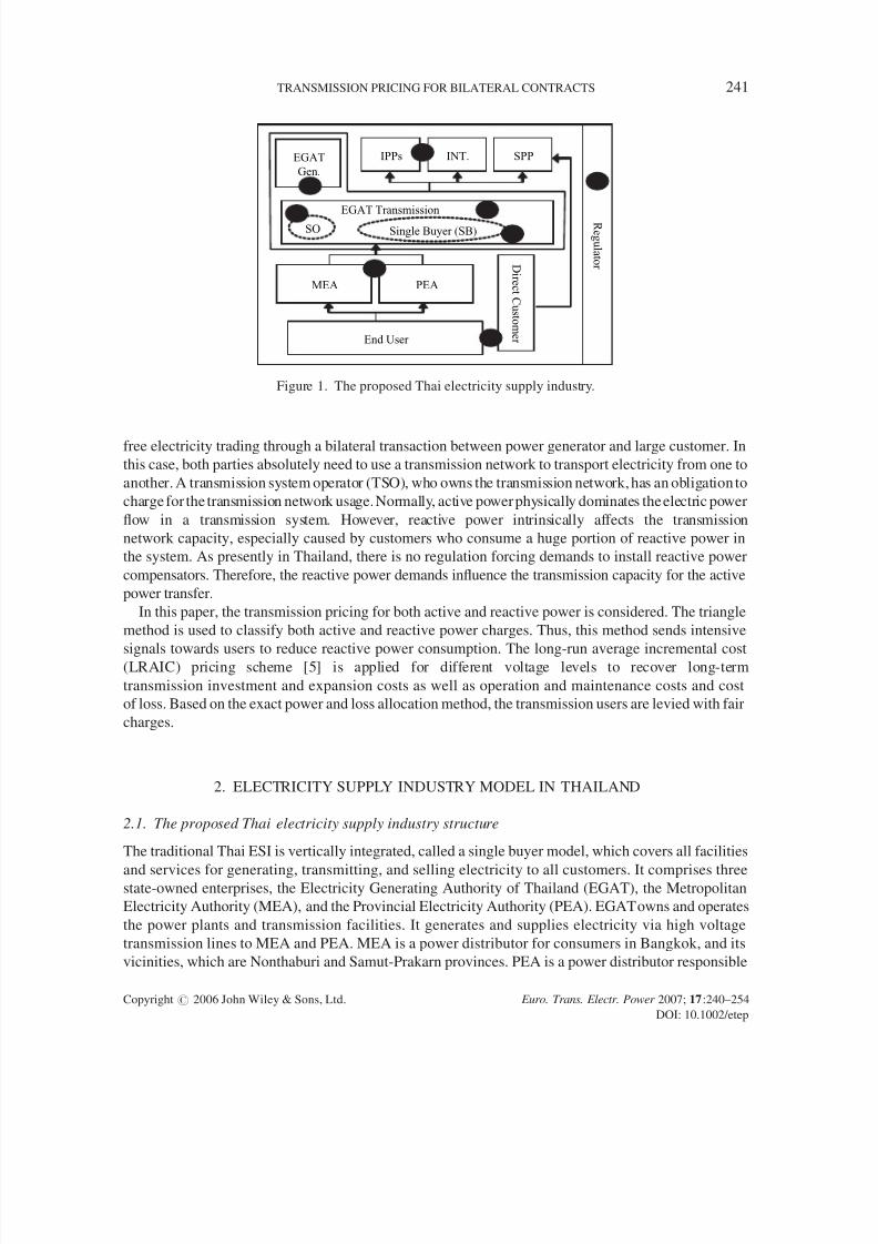
model in 2002 [2], and lastly the enhanced single buyer (ESB) model in 2003 [3,4] that is currentlyrecommended to apply with the present Thai ESI. The ESB model, as shown in Figure 1, encourages

EUROPEAN TRANSACTIONS ON ELECTRICAL POWEREuro. Trans. Electr. Power 2007; 17:240–254Published online 30 November 2006 in Wiley InterScience(www.interscience.wiley.com) DOI: 10.1002/etep.131

*Correspondence to: Weerakorn Ongsakul, Energy Field of Study, School of Environment, Resources and Development, AsianInstitute of Technology, Pathumthani 12120, Thailand.yE-mail: [email protected]

Copyright# 2006 John Wiley & Sons, Ltd.



free electricity trading through a bilateral transaction between power generator and large customer. In

this case, both parties absolutely need to use a transmission network to transport electricity from one to

another. A transmission system operator (TSO), who owns the transmission network, has an obligation to

charge for the transmission network usage. Normally, active power physically dominates the electric power

flow in a transmission system. However, reactive power intrinsically affects the transmission

network capacity, especially caused by customers who consume a huge portion of reactive power in

the system. As presently in Thailand, there is no regulation forcing demands to install reactive power

compensators. Therefore, the reactive power demands influence the transmission capacity for the active

power transfer.

In this paper, the transmission pricing for both active and reactive power is considered. The triangle

method is used to classify both active and reactive power charges. Thus, this method sends intensive

signals towards users to reduce reactive power consumption. The long-run average incremental cost(LRAIC) pricing scheme [5] is applied for different voltage levels to recover long-term

transmission investment and expansion costs as well as operation and maintenance costs and cost

of loss. Based on the exact power and loss allocation method, the transmission users are levied with fair

charges.

2. ELECTRICITY SUPPLY INDUSTRY MODEL IN THAILAND

2.1. The proposed Thai electricity supply industry structure

The traditional Thai ESI is vertically integrated, called a single buyer model, which covers all facilities

and services for generating, transmitting, and selling electricity to all customers. It comprises threestate-owned enterprises, the Electricity Generating Authority of Thailand (EGAT), the Metropolitan

Electricity Authority (MEA), and the Provincial Electricity Authority (PEA). EGATowns and operates

the power plants and transmission facilities. It generates and supplies electricity via high voltage

transmission lines to MEA and PEA. MEA is a power distributor for consumers in Bangkok, and its

vicinities, which are Nonthaburi and Samut-Prakarn provinces. PEA is a power distributor responsible

EGAT

Gen.

IPPs INT. SPP

PEA

r e m o t s u C t c e r i D r

o t a l u g e R

EGAT Transmission

SO Single Buyer (SB)

End User

MEA

Figure 1. The proposed Thai electricity supply industry.

Copyright# 2006 John Wiley & Sons, Ltd. Euro. Trans. Electr. Power 2007; 17:240–254

DOI: 10.1002/etep

TRANSMISSION PRICING FOR BILATERAL CONTRACTS 241



for consumers in the remaining regions of Thailand. This traditional structure lacks of the competition

and efficiency, consequently over investments and low efficiency take place in any sectors. The Energy

Policy and Planning Office (EPPO), which regulates the three enterprises, has decided to restructure the

traditional Thai ESI.

Since 2003, EPPO has proposed the ESB model aiming to increase efficiency-drivers to the common

single buyer model of the Thai ESI. The key objectives of this model are:

Improving security of supply with high grid reliability and adequate generation;

Increasing customer satisfaction; in the generation sector by increasing efficiency on the use of

energy and financial resources, more choices on competition, transparent, and competitive tariffs;

in the customer sector by increasing service quality with stable power prices;

Maintaining social and environment obligations;

Creating national champions with economies of scale consideration; and

Operating with low risk and cost of transition.

In the ESB model shown in Figure 1, the main characteristics of the Thai ESI have been changed.

They are classified into eight issues as follows. (1) EGAT still holds generation and transmission

services. However, there will be an account unbundling of both business units. (2) In the generation

sector, the new capacity will be allocated through the process and the market regulation determined by

the regulator. (3) EGAT retains the transmission network with regulated tariffs and has responsibility

for both network operations and maintenance. The transmission network will be regulated via the Grid

Code and transmission license. (4) The System Operator (SO) will be ring-fenced within EGAT as well

as it will retain obligation for dispatch planning, dispatch, real time balancing and network

operations planning. (5) Single Buyer (SB) will be transparent within transmission service and

responsible for contracting adequate transmission capacity and accountable for long-term system

adequacy planning. (6) MEA and PEA will continue to operate their networks with regulated tariffs via

the Grid Code and distribution license. (7) End user tariffs will continue to be regulated by the

regulator. (8) The Regulator will enforce the Grid Code and generation as well as transmission and

distribution licenses.

This model encourages independent power producers (IPPs) and small power producers (SPPs) toparticipate in the generation sector, while it allows large customers to select their own suppliers. Both

of them are able to enter into bilateral contracts, which are individually negotiated between two parties

in order to achieve price stability and to ensure sufficient electricity supply. This method becomes more

efficient and provides market participants more choices while maintaining the operation of a secure and

reliable electricity system. The SO has the function to support for transmission services and a privilege

for transmission service charges.

3. POWER AND LOSS ALLOCATION METHOD FOR BILATERAL CONTRACTS

A bilateral contract is a long-term physical contract between participants to purchase and sale energy.

The transmission network is used to transfer both active and reactive power from a generator as seller toa load as buyer in a bilateral contract. The transmission power and loss allocation become a major

concern for market participants. In case of Thailand, which has high reactive power consumption, the

transmission owner needs to support a portion of transmission capacity for reactive power delivering. It

decreases the transmission capacity for the active power transfer. Consequently, it needs a charge to the

user, who has a huge reactive power demand. In this section, the exact power and loss allocation for a


DOI: 10.1002/etep

242 C. ADSOONGNOEN ET AL.



bilateral contract in the ESB model are presented. Both active and reactive power allocations are taken

into consideration.

3.1. Review of transmission power/energy and loss allocation methods

In different electricity market environments, many methods have been proposed to allocate power,

energy, and losses for transmission system service charges to make fair charges to market participants.

The load flow based on loss allocation method [6] traces the specific component load flow on a

distribution system. The losses are allocated to customers using the evaluation of loss adjustment

factors at a specific location. However, this method depends on a slack bus. It is only applicable to radial

distribution networks, and has no incentive for loss reduction. Optimal power flow based on

incremental loss evaluation method [7,8] has been applied to the bilateral transaction in a transmission

system that is independent of a slack bus. The concept accounts for the transaction injection charges of

both sending and sinking buses. However, it encounters a transaction-sequence problem. Thus, it is

time-consuming.

In Reference [9], two different sensitivity factors for transmission pricing based on the loss

estimation method have been proposed, called a generalized generation distribution factor and ageneralized load distribution factor, which depend on standard load flow. They have been proposed to

allocate transmission losses and marginal operating costs of individual transaction. The sensitivity

factors are computationally efficient. The loss penalty factor in Reference [10] has been introduced to

evaluate wheeling losses by using a constant nodal matrix and known-operating point. However, it

creates unsatisfied results for the large system comprising many transactions. Both distribution factors

and loss penalty factor are closely related to a slack bus.

The tracing method is implemented to allocate energy and losses to a particular load and generator. It

is based on proportional-sharing providing signals to recover the transmission network costs while

minimizing distortion and interference of economic efficiency [11]. The tracing results have shown that

methodology is simple, fair, and transparent. Therefore, this method has been proposed for the

transmission pricing in the Thai power pool model as given in Reference [12,13]. However, it seems to

be time-consuming for a large system.A loss distribution based on power flow method has been proposed to calculate transmission losses

and associated costs for bilateral transactions in a deregulated environment [14,15]. The method

achieves a fair loss allocation, and the allocated results are independent of the selecting of slack bus.

Both, positive and negative losses are accounted for leading to economic efficiency. However, only

active power and allocated active losses have been considered so far. This paper aims to develop the

reactive power and reactive loss allocation for bilateral contracts. The results are used to calculate the

transmission pricings for active power, reactive power and associated losses.

3.2. The proposed power and loss allocation method

The algorithm to allocate active and reactive power with associated losses for each bilateral transactioninitially takes a Newton-Raphson power flow calculation. Thereafter, the allocation method will be

applied to the transaction. The method starts with an identification of transaction pairs, which consists

of a sending bus and its associated receiving bus. The demand of each transaction must be given.

The ideal transaction pair is self-balancing so that its net power generation is equal to the sum of its

demand and loss. In this paper, a single transaction is simplified. The nodal power balance equations are


DOI: 10.1002/etep




shown in Equations (1–3).

For each k

2 ns

Pk ¼ U k

Pn

j¼1

U jðGkj cos dkj þ Bkj sin dkjÞ

Qk ¼ U k Pn

j¼1 U jðGkj sind

kj Bkj cosd

kjÞdkj ¼ dk d j

8>>>><>>>>:

(1)

For each m 2 nb

Pm ¼ U mPn

j¼1

U jðGmj cos dmj þ Bmj sin dmjÞ

Qm ¼ U mPn

j¼1

U jðGmj sin dmj Bmj cos dmjÞdmj ¼ dm d j

8>>>><>>>>:

(2)

For each l 2

nz

0 ¼ U lPn

j¼1

U jðGlj cos dlj þ Blj sin dljÞ

0 ¼ U lPn

j¼1U jðGlj sin dlj Blj cos dljÞ

dlj ¼ dl d j

8>>>><>>>>:

(3)

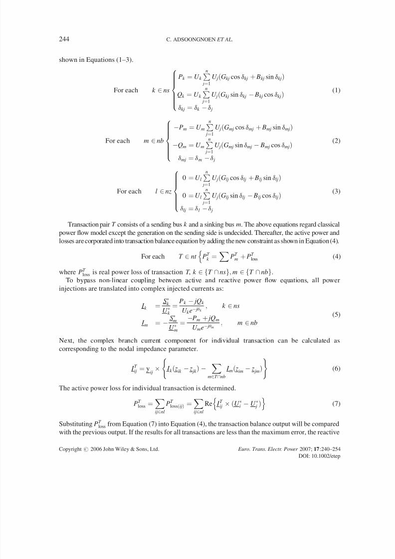
Transaction pair T consists of a sending bus k and a sinking bus m. The above equations regard classical

power flow model except the generation on the sending side is undecided. Thereafter, the active power and

losses are corporated into transaction balance equation by adding the new constraint as shown in Equation (4).

For each T 2 nt PT k ¼

XPT

m þ PT loss

n (4)

where PT loss is real power loss of transaction T , k 2 T \ nsf g; m 2 T \ nbf g.

To bypass non-linear coupling between active and reactive power flow equations, all power

injections are translated into complex injected currents as:

I k ¼ S k

U k

¼ Pk jQk

U k e ju k ; k 2 ns

I m ¼ S mU m

¼ Pm þ jQm

U me ju m; m 2 nb

(5)

Next, the complex branch current component for individual transaction can be calculated as

corresponding to the nodal impedance parameter.

I T ij ¼ y

ij I k ð zik z jk Þ

Xm2T \nb

I mð zim z jmÞ( )

(6)

The active power loss for individual transaction is determined.

PT loss ¼

Xij2nl

PT lossðijÞ ¼

Xij2nl

Re I T ij ðU i U j Þ

n o (7)

Substituting PT loss from Equation (7) into Equation (4), the transaction balance output will be compared

with the previous output. If the results for all transactions are less than the maximum error, the reactive


DOI: 10.1002/etep




power consumption QT

loss for each transaction is calculated in an analogous way as given inEquation (8).

QT loss ¼

Xij2nl

QT lossðijÞ ¼

Xij2nl

Im I T ðijÞ ðU i U j Þ

n o (8)

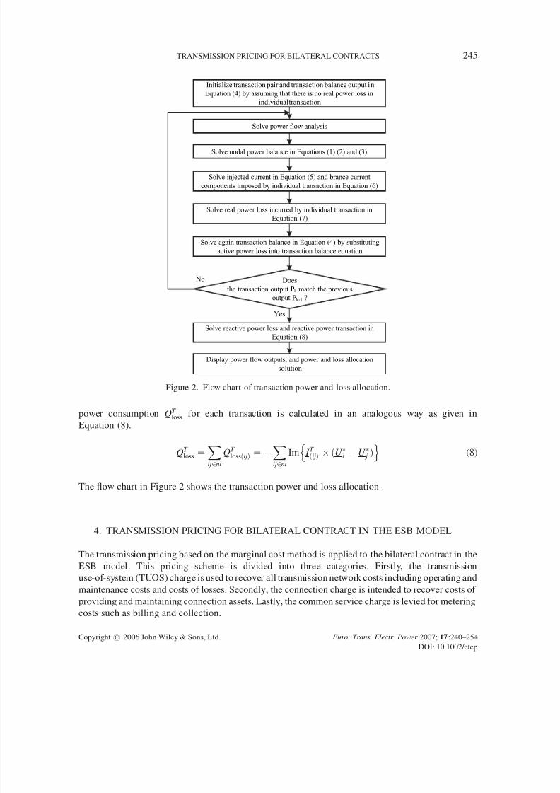
The flow chart in Figure 2 shows the transaction power and loss allocation.

4. TRANSMISSION PRICING FOR BILATERAL CONTRACT IN THE ESB MODEL

The transmission pricing based on the marginal cost method is applied to the bilateral contract in theESB model. This pricing scheme is divided into three categories. Firstly, the transmission

use-of-system (TUOS) charge is used to recover all transmission network costs including operating and

maintenance costs and costs of losses. Secondly, the connection charge is intended to recover costs of

providing and maintaining connection assets. Lastly, the common service charge is levied for metering

costs such as billing and collection.

Does

the transaction output Pk match the previous

output Pk-1 ?

Solve power flow analysis

Solve nodal power balance in Equations (1) (2) and (3)

Solve injected current in Equation (5) and brance current

components imposed by individual transaction in Equation (6)

Solve real power loss incurred by individual transaction in

Equation (7)

Solve again transaction balance in Equation (4) by substituting

active power loss into transaction balance equation

Solve reactive power loss and reactive power transaction in

Equation (8)

Display power flow outputs, and power and loss allocation

solution

Yes

No

Initialize transaction pair and transaction balance output in

Equation (4) by assuming that there is no real power loss in

individual transaction

Figure 2. Flow chart of transaction power and loss allocation.


DOI: 10.1002/etep




4.1. The transmission use-of-system charge (TUOS)

The TUOS charge reflects network investments and operating costs. This charge involves power and

loss charges paid by customers at the extracting points. LRAIC is proposed to determine the

transmission tariffs. There are the uniform tariffs for different voltage levels based on a cost-roll-over

method, which take the marginal capacity costs and the marginal transmission losses into account. The

marginal transmission losses for different voltage levels are given in Table I. LRAIC is calculated as

given in Equation (9).

LRAICi ¼ CT i

DM i(9)

where DM i is a discounted projection of new demands at each voltage level for future years, CT i is a

discounted optimal-incremental investment required to meet the new demand, and i is the voltage level.

These costs should be allocated between 9 a.m. and 10 p.m., the peak period at all weekdays (except

public holidays) over all months of the year. The calculation is based on the basis of 20-year payback

with 7% discount rate and currency exchange rate of 36 BHT ¼ 1 USD. The detailed data of LRAIC

calculation is given in Reference [5]. The LRAIC results are shown in Table II for each voltage level.

These tariffs consider only active power charge based on an average EGAT’s system power factor 0.8.

However, this system contains high reactive loads, which requires a portion of transmission capacities. As

a result, only active power charge cannot achieve the expected revenue requirement. Thus, this paperextends the transmission use-of-system charge to the reactive power pricing. The authors propose the

triangle method to allocate active power and reactive power charges (MW- and MVar-charges).

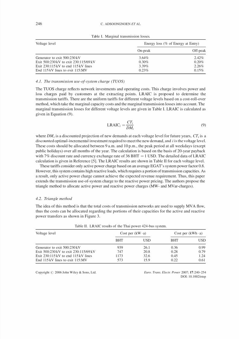
4.2. Triangle method

The idea of this method is that the total costs of transmission networks are used to supply MVA flow,

thus the costs can be allocated regarding the portions of their capacities for the active and reactive

power transfers as shown in Figure 3.

Table I. Marginal transmission losses.

Voltage level Energy loss (% of Energy at Entry)

On-peak Off-peak

Generator to exit 500:230 kV 3.64% 2.42%Exit 500:230 kV to exit 230:115/69 kV 0.30% 0.20%Exit 230:115 kV to end 115 kV lines 3.39% 2.26%End 115 kV lines to exit 115:MV 0.23% 0.15%

Table II. LRAIC results of the Thai power 424-bus system.

Voltage level Cost per (kW

a) Cost per (kWh

a)

BHT USD BHT USD

Generator to exit 500:230 kV 939 26.1 0.36 0.99Exit 500:230 kV to exit 230:115/69 kV 747 20.8 0.28 0.79Exit 230:115 kV to end 115 kV lines 1173 32.6 0.45 1.24End 115 kV lines to exit 115:MV 573 15.9 0.22 0.61


DOI: 10.1002/etep




The complex power is separated to be active and reactive power by using the relationship

S 2¼ P

2þ Q2

. Assuming that the total transmission costs based on MVA, Cost (S ) can also be

transformed into both costs supporting active power transfer, Cost (P) and reactive power transfer,Cost

(Q) as given in Equations (10) and (11).

Cost ðPÞ ¼ Cost ðS Þ P

S (10)

and

Cost ðQÞ ¼ Cost ðS Þ ffiffiffiffiffiffiffiffiffiffiffi ffiffiffiffiffi

S 2 P2p

S

! (11)

From the equations above, we obtain the cost-relation result as Cost (P) þ Cost (Q) i Cost (S ), which is

unreasonable because the total revenue from active and reactive power transfer is greater than the total

costs of the transmission network. Thus, the cosine rule in Equation (12) is applied to allocate the new

costs, which would not exceed the total revenue requirement. The new allocated costs for active and

reactive power transfer are expressed in Equations (13) and (14).

cos2 u þ sin2 u ¼ 1 (12)

Cost ðP0Þ ¼ Cost ðS Þ cos2u (13)

Cost ðQ0Þ ¼ Cost ðS Þ sin2u (14)

Using Equations (13) and (14), LRAIC is reallocated with the power factor 0.8. The new LRAIC for

active power and reactive power transfer are shown in Tables III and IV, respectively.

Cost ( P )

θ

t s o C

( Q )

C o s t (

P ’ )

C o s t (

Q ’ )

Figure 3. Triangle method for the active and reactive power allocation.

Table III. The allocated LRAIC for active power transfer.

Voltage level Cost per (kW

a) Cost per (kWh

a)

BHT USD BHT USD



DOI: 10.1002/etep




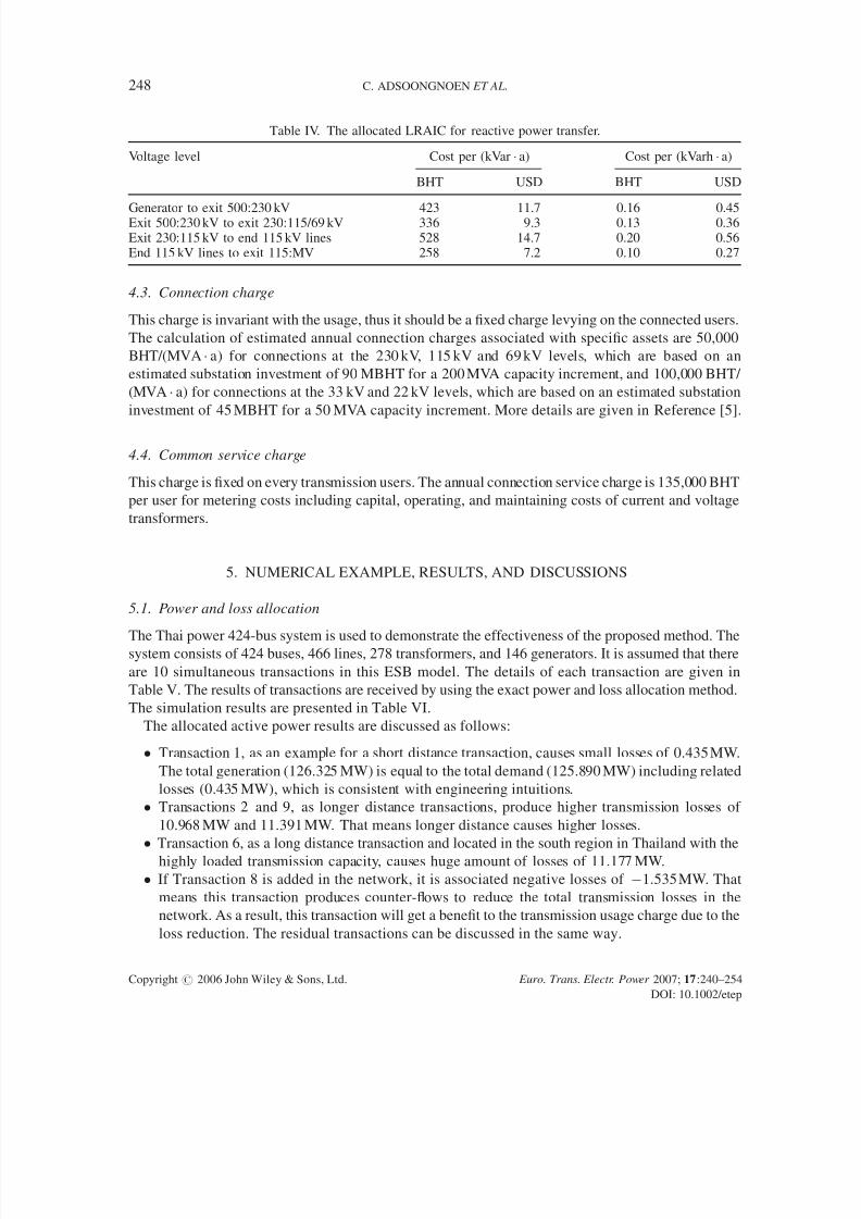
4.3. Connection charge

This charge is invariant with the usage, thus it should be a fixed charge levying on the connected users.

The calculation of estimated annual connection charges associated with specific assets are 50,000

BHT/(MVA a) for connections at the 230 kV, 115 kV and 69 kV levels, which are based on an

estimated substation investment of 90 MBHT for a 200 MVA capacity increment, and 100,000 BHT/

(MVA a) for connections at the 33 kV and 22 kV levels, which are based on an estimated substation

investment of 45 MBHT for a 50 MVA capacity increment. More details are given in Reference [5].

4.4. Common service charge

This charge is fixed on every transmission users. The annual connection service charge is 135,000 BHT

per user for metering costs including capital, operating, and maintaining costs of current and voltage

transformers.

5. NUMERICAL EXAMPLE, RESULTS, AND DISCUSSIONS

5.1. Power and loss allocation

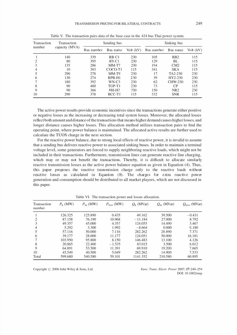
The Thai power 424-bus system is used to demonstrate the effectiveness of the proposed method. Thesystem consists of 424 buses, 466 lines, 278 transformers, and 146 generators. It is assumed that there

are 10 simultaneous transactions in this ESB model. The details of each transaction are given in

Table V. The results of transactions are received by using the exact power and loss allocation method.

The simulation results are presented in Table VI.

The allocated active power results are discussed as follows:

Transaction 1, as an example for a short distance transaction, causes small losses of 0.435 MW.

The total generation (126.325 MW) is equal to the total demand (125.890 MW) including related

losses (0.435 MW), which is consistent with engineering intuitions.

Transactions 2 and 9, as longer distance transactions, produce higher transmission losses of

10.968 MW and 11.391 MW. That means longer distance causes higher losses.

Transaction 6, as a long distance transaction and located in the south region in Thailand with the

highly loaded transmission capacity, causes huge amount of losses of 11.177 MW.

If Transaction 8 is added in the network, it is associated negative losses of 1.535 MW. That

means this transaction produces counter-flows to reduce the total transmission losses in the

network. As a result, this transaction will get a benefit to the transmission usage charge due to the

loss reduction. The residual transactions can be discussed in the same way.

Table IV. The allocated LRAIC for reactive power transfer.

Voltage level Cost per (kVar a) Cost per (kVarh a)

BHT USD BHT USD



DOI: 10.1002/etep




The active power results provide economic incentives since the transactions generate either positive

or negative losses as the increasing or decreasing total system losses. Moreover, the allocated losses

reflect both amount and distance of the transactions that means higher demand causes higher losses, and

longer distance causes higher losses. This allocation method utilizes transaction pairs to find the

operating point, where power balance is maintained. The allocated active results are further used to

calculate the TUOS charge in the next section.

For the reactive power balance, due to strong local effects of reactive power, it is invalid to assume

that a sending bus delivers reactive power to associated sinking buses. In order to maintain a terminal

voltage level, some generators are forced to supply neighboring reactive loads, which might not be

included in their transactions. Furthermore, transmission lines can generate reactive line charging,

which may or may not benefit the transactions. Thereby, it is difficult to allocate similarly

reactive transmission losses as the active power balance equation as given in Equation (4). Thus,

this paper proposes the reactive transmission charge only to the reactive loads without

reactive losses as calculated in Equation (8). The charges for extra reactive powergeneration and consumption should be distributed to all market players, which are not discussed in

this paper.

Table V. The transaction pairs data of the base case in the 424 bus Thai power system.

Transactionnumber

Transactioncapacity (MVA)

Sending bus Sinking bus

Bus number Bus name Volt (kV) Bus number Bus name Volt (kV)

1 140 339 RB-C1 230 105 RB2 1152 80 395 RY-C1 230 129 BL 1153 135 286 MM-T7 230 194 CM2 1154 10 383 COCO-T1 115 341 SKA 1155 290 278 MM-T9 230 17 TA2-230 2306 130 274 RPB-H1 230 39 HY2-230 2307 180 392 WN-C3 230 62 CHW-230 2308 90 400 TOP-T1 230 73 CP 1159 90 366 HH-H2 230 150 NR2 230

10 290 378 BCC-T1 115 332 SNR 115

Table VI. The transaction power and losses allocation.

Transactionnumber

Pk (MW) Pm (MW) Ploss (MW) Qk (MVar) Qm (MVar) Qloss (MVar)

1 126.325 125.890 0.435 49.162 39.500 0.4312 87.158 76.190 10.968 11.184 27.000 8.7923 49.357 45.000 4.357 124.055 14.490 3.4674 5.292 3.300 1.992 8.664 0.000 0.1805 57.116 50.000 7.116 282.262 28.890 7.371

6 39.177 28.000 11.177 124.051 50.000 16.1817 103.950 95.800 8.150 146.483 13.100 4.1268 20.865 22.400 1.535 83.015 3.500 6.0129 64.891 53.500 11.391 69.910 19.200 7.665

10 45.549 40.500 5.049 282.262 14.900 7.533Total 599.680 540.580 59.101 1141.352 210.580 60.895


DOI: 10.1002/etep




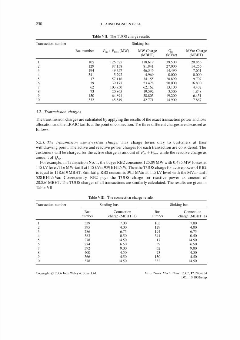
5.2. Transmission charges

The transmission charges are calculated by applying the results of the exact transaction power and lossallocation and the LRAIC tariffs at the point of connection. The three different charges are discussed as

follows.

5.2.1. The transmission use-of-system charge. This charge levies only to customers at their

withdrawing point. The active and reactive power charges for each transaction are considered. The

customers will be charged for the active charge as amount of Pmþ Ploss while the reactive charge as

amount of Qm.

For example, in Transaction No. 1, the buyer RB2 consumes 125.89 MW with 0.435 MW losses at

115 kV level. The MW-tariff at 115 kVis 939 BHT/kW. Then the TUOS charge for active power of RB2

is equal to 118.619 MBHT. Similarly, RB2 consumes 39.5 MVar at 115 kV level with the MVar-tariff

528 BHT/kVar. Consequently, RB2 pays the TUOS charge for reactive power as amount of 20.856 MBHT. The TUOS charges of all transactions are similarly calculated. The results are given in

Table VII.

Table VII. The TUOS charge results.

Transaction number Sinking bus

Bus number Pmþ Ploss (MW) MW-Charge(MBHT)

Qm

(MVar)MVar-Charge

(MBHT)

1 105 126.325 118.619 39.500 20.8562 129 87.158 81.841 27.000 14.2563 194 49.357 46.346 14.490 7.6514 341 5.292 4.969 0.000 0.0005 17 57.116 34.155 28.890 9.7076 39 39.177 23.428 50.000 16.8007 62 103.950 62.162 13.100 4.4028 73 20.865 19.592 3.500 1.8489 150 64.891 38.805 19.200 6.451

10 332 45.549 42.771 14.900 7.867

Table VIII. The connection charge results.

Transaction number Sending bus Sinking bus

Busnumber

Connectioncharge (MBHT a)

Busnumber

Connectioncharge (MBHT a)

1 339 7.00 105 7.002 395 4.00 129 4.003 286 6.75 194 6.754 383 0.50 341 0.505 278 14.50 17 14.506 274 6.50 39 6.507 392 9.00 62 9.008 400 4.50 73 4.509 366 4.50 150 4.50

10 378 14.50 332 14.50


DOI: 10.1002/etep




5.2.2. The connection charge. The costs of connection are based on the costs of facilities that are used

to join the transmission users with the network. Therefore, both sellers and buyers are willing to pay for

these connection charges. The connection charge is based on the annual maximum MVA of each

transaction. As presented in Table V, all users are connected at the voltage levels 115 kV and 230 kV.

Therefore, the connection tariff is 50 000 BHT/(MVA

a). The connection charge results are calculated

by multiplying this tariff with the committed transaction capacity in Table V. The results are given in

Table VIII.

5.2.3. The common service charge. As mentioned in Section 4.3, all users pay for this service charge

135 000 BHT annually to cover the metering, billing, and collection services.

6. CONCLUSIONS

This paper presents a transmission pricing for the bilateral market in the Thai ESI. The transmission

pricing comprises three categories as the transmission use-of-system charge, the connection charge,

and the common service charge. The transmission use-of-system charge is determined by using theexact power and loss allocation method and the triangle method for active and reactive power transfers

committed by transaction pairs in the bilateral market to recover the related network costs. Then active

and reactive transmission charges for each transaction are allocated. Similarly, the connection charge

and the common service charge are used to recover the residual facilities costs and the costs of

administration. The users are charged regarding their system usage. To examine its effectiveness, the

proposed method is applied to the Thai 424-bus system. The simulation results prove that the proposed

pricing method for the use-of-system charge sends correct economic incentives to the users by

penalizing long distance transfer over highly loaded lines and rewarding transfer that reduces network

loading and system losses. Moreover, the tariffs fairly reflect the effects on both quantities and distance

of any transaction. Similarly, the other charges collect the residual annually fixed costs.

7. LIST OF SYMBOLS, SUBSCRIPTS, AND ABBREVIATIONS

Symbolsa per year

n set of all bus in the system (n ¼ nz þ nb þ ns)

ns set of sending buses

nb set of sinking buses

nz set of nodes with zero net injection

nl set of all branches (lines and transformers)

nt set of bilateral transactions

X complex number

X

conjugationU voltage

S bus power

P active power

Q reactive power

I injection current


DOI: 10.1002/etep




y admittance

z impedance

Cost cost

CT discounted incremental investment

DM discounted projection of new demand

Subscriptsi,j,k,l,n,m identified buses

loss loss

T bilateral transaction

d, u angle

AbbreviationsBHT Thai Baht

EGAT Electricity Generating Authority of Thailand

EPPO Energy Policy and Planning Office

ESB Enhanced single buyer

ESI Electricity supply industry

IPP Independent power producer

LRAIC Long run average incremental cost

MEA Metropolitan Electricity Authority

NESA New electricity supply arrangement

PEA Provincial Electricity Authority

SB Single buyer

SO System operator

SPP Small power producer

TSO Transmission system operator

TUOS Transmission use-of-system

REFERENCES

1. Energy Policy and Planning Office of Thailand. Thailand power pool and electricity supply industry reform study-phase Ifinal report, available at http://www.eppo.go.th/power/pw-PowerPool-FR-index.html 2000; March.

2. Energy Policy and Planning Office of Thailand. Electricity supply industry restructuring plan. 2002.3. Ministry of Energy, Royal Thai Government. The structure of electricity supply industry. 2003; December.4. Electricity Generating Authority of Thailand. Restructuring of the Thai electricity supply industry and regulation . 2004;

May.5. Energy Policy and Planning Office of Thailand. Review of electric power tariffs-final report, available at http://

www.eppo.go.th/power/pw-FR3-index.html 2000; January.6. Macqueen CN, Irving MR. An algorithm for the allocation of distribution system demand and energy losses. IEEE

Transactions on Power Systems 1996; 11(1):338–343.7. Happ HH. Cost of wheeling methodologies. IEEE Transactions on Power Systems 1994; 9(1):147–156.8. Shirmohammadi D, Filho XV, Gorenstin B, Pereira MVP. Some fundamental technical concepts about cost based

transmission pricing. IEEE Transactions on Power Systems 1996; 11(2):1002–1008.9. Rudnick H, Palma R, Fernandez JE. Marginal pricing and supplement cost allocation in transmission open access. IEEE

Transactions on Power Systems 1995; 10(2):1125–1142.10. Clayton JS, Ewin SR, Gibson CA. Interchange costing and wheeling loss evaluation by means of incremental. IEEE

Transactions on Power Systems 1990; 5(3):759–765.


DOI: 10.1002/etep




11. Bialek JW. Tracing the flow of electricity. IEE Proceeding Generation, Transmission and Distribution 1996;143(4):313–320.

12. Limpasuwan T, Bialek JW, Ongsakul W, Limmeechokchai B. A proposal for annual power fee in Thailand based onelectricity tracing methodology. Electric Power Systems Research 2003; 64:219–226.

13. Limpasuwan T, Bialek JW, Ongsakul W, Limmeechokchai B. A proposal for transmission pricing methodology in Thailandbased on electricity tracing and long-run average incremental cost. Energy Policy 2004; 32(3):301–308.

14. Huang GM, Zhang H. Transmission loss allocations and pricing via bilateral energy transaction. IEEE Power EngineeringSociety Summer Meeting 1999; 2:720–725.

15. Ongsakul W, Adsoongnoen C. A proposal for transmission pricing methodology in Thailand based on exact loss contributionand long-run average incremental cost. International Energy Journal 2005; 6(1.2): 29–42.

AUTHORS’ BIOGRAPHIES

Cattareeya Adsoongnoen was born in Nakhon Ratchasima, Thailand in 1976. She receivedher B.Eng. degree from Khon Kaen University, Khon Kaen, Thailand in 1998 and M.Eng.degree from Asian Institute of Technology, Thailand in 2002. She is a lecturer at Faculty of Engineering, Naresuan University. Currently, she is a doctoral student in Energy Field of Study, School of Environment, Resources and Development, Asian Institute of Technology,Thailand, and the exchange student under joint supervision at the Institute of Power Systems

and Power Economics, RWTH Aachen University, Germany. Her research interests includeelectricity market, power economics and transmission pricing. Her address is Institute of Power Systems and Power Economics, RWTH Aachen University, Schinkelstr.6, Aachen52056, Germany.

Weerakorn Ongsakul was born in Thailand in 1967. He received his B.Eng. degree fromChulalongkorn University, Bangkok, Thailand in 1988, and M.S. degree in 1991 and Ph.D.degree in 1994 in Electrical Engineering from Texas A&M University, College Station,Texas, USA. Currently, he is an Associate Professor at the Energy Field of Study, AsianInstitute of Technology, Thailand. His interests are in computer applications to power system,parallel processing applications, AI applications to power systems, and power systemrestructuring and deregulation. His address is Energy Field of Study, School of Environment,

Resources and Development, Asian Institute of Technology, Pathumthani 12120, Thailand.

Christoph Maurer was born in Mayen, Germany in 1977. He is the chief engineer at theInstitute of Power Systems and Power Economics, RWTH Aachen University, Germany. Hereceived his Dipl.-Ing. in 2001 and Dr.-Ing. in 2004 from RWTH Aachen University, andDipl.-Wirt.-Ing. in 2005 from Hagen University. His research interests are in the optimizationtechniques for network planning and operation, regulation and development of electricitymarkets. His address is Institute of Power Systems and Power Economics, RWTH AachenUniversity, Schinkelstr.6, Aachen 52056, Germany.


DOI: 10.1002/etep




Hans-Ju ¨ rgen Haubrich was born in Montabaur, Germany in 1941. He received his Dipl.-Ing.from Darmstadt University of Technology in 1965. Thereafter, he was a member of scientificstaff at the Institute of Electrical Energy Supply of Darmstadt University of Technology wherehe received his Dr.-Ing. in 1971. During 1971–1973, he was a freelancer for Brown BoveryAG, Mannheim, Germany and during 1973–1998 he was member of the VEW staff,Dortmund, Germany, finally as the head of the Central Planning Department. In 1985 hewas appointed as a honorary professor at University Bochum. Since 1990 he has been theProfessor and the head of the Institute of Power Systems and Power Economics at RWTHAachen University. Since 1997 he is an additional member of the Academy of Science of thefederal state North-Rhine Westphalia and since 2003 he has been the director of the‘Forschungsgemeinschaft fur Elektrische Anlagen und Stromwirtschaft e.V.’ (FGH), Man-nheim.


DOI: 10.1002/etep


Documents

Transmission Pricing 37