TRANSPORTATION RESEARCH

RECORD No. 1489

Rail

Railroad Transportation Research

A peer-reviewed publication of the Transportation Research Board

TRANSPORTATION RESEARCH BOARD NATIONAL RESEARCH COUNCIL

NATIONAL ACADEMY PRESS WASHINGTON, D.C. 1995

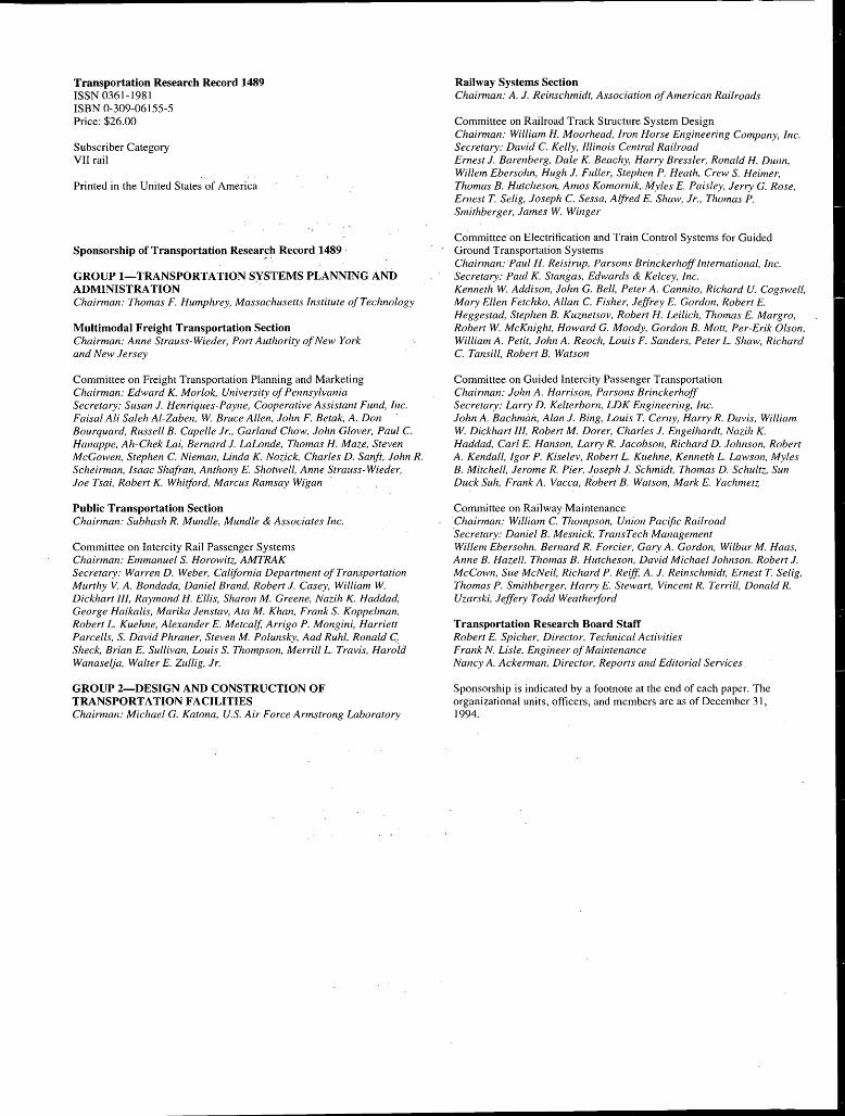
Transportation Research Record 1489 ISSN 0361-1981 ISBN 0-309-06155-5 Price: $26.00

Subscriber Category VII rail

Printed in the United States of America

Sponsorship of Transportation Resear~h Record 1489 ·

GROUP I-TRANSPORTATION SYS.TEMS PLANNING AND ADMINISTRATION Chairman: Thomas F. Humphrey, Massachusetts Institute of Technology

Multimodal Freight Transportation Section Chairman: Anne Strauss-Wieder, Port Authority of New York and New Jersey

Committee on Freight Transportation Planning and Marketing Chairman: Edward K. Morlok, University of Pennsylvania Secretary: Susan J. Henriques-Payne, Cooperative Assistant Fund, Inc. Faisal Ali Saleh Al-Zaben, W. Bruce Allen, John F. Betak, A. Don · Bourquard, Russell B. Cape/le Jr., Garland Chow, John Glover, Paul C. Hanappe, Ah-Chek Lai, Bernard J. LaLonde, Thomas H. Maze, Steven McGowen, Stephen C. Nieman, Linda K. Nozick, Charles D. Sanft, John R. Scheirman, Isaac Shafran, Anthony E. Shotwell, Anne Strauss-Wieder, Joe Tsai, Robert K. Whitford, Marcus Ramsay Wigan ·

Public Transportation Section Chairman: Subhash R. Mundie, Mundie & Associates Inc.

Committee on Intercity Rail Passenger Systems Chairman: Emmanuel S. Horowitz, AMTRAK Secretary: Warren D. Weber, California Department of Transportation Murthy V. A. Bondada, Daniel Brand, Robert J. Casey, William W. Dickhart III, Raymond H. Ellis, Sharon M. Greene, Nazih K. Haddad, George Haikalis, Marika Jenstav, Ata M. Khan, Frank S. Koppelman, Robert L. Kuehne, Alexander E. Metcalf. Arrigo P. Mangini, Harriett Parcells, S. David Phraner, Steven M. Polunsky, Aad Ruhl, Ronald C..:.. Sheck, Brian E. Sullivan, Louis S. Thompson, Merrill L. Travis, Harold Wanaselja, Walter E. Zullig, Jr.

GROUP 2-DESIGN AND CONSTRUCTION OF TRANSPORTATION FACILITIES Chairman: Michael G. Katona, U.S. Air Force Armstrong Laboratory

Railway Systems Section Chairman: A. J. Reinschmidt, Association of American Railroads

Committee on Railroad Track Structure System Design Chairman: William H. Moorhead, Iron Horse Engineering Company, Inc. Secretary: David C. Kelly, Illinois Central Railroad Ernest J. Barenberg, Dale K. Beachy, Harry Bressler, Ronald H. Dunn, Willem Ebersohn, Hugh J. Fuller, Stephen P. Heath, Crew S. Heimer, Thomas B. Hutcheson, Amos Komornik, Myles E. Paisley, Jerry G. Rose, Ernest T. Selig, Joseph C. Sessa, Alfred E. Shaw, Jr., Thomas P. Smithberger, James W. Winger

Committee on Electrification and Train Control Systems for Guided Ground Transportation Systems Chairman: Paul H. Reisirup, Parsons Brinckerhoff International, Inc. Secretary: Paul K. Stangas, Edwards & Kelcey, Inc. Kenneth W. Addison, John G. Bell, Peter A. Cannito, Richard U. Cogswell, Mary Ellen Fetchko, Allan C. Fisher, Jeffrey E. Gordon, Robert E. Heggestad, Stephen B. Kuznetsov, Robert H. Leilich, Thomas E. Margro, Robert W. McKnight, Howard G. Moody, Gordon B. Mott, Per-Erik Olson. William A. Petit, John A. Reach, Louis F. Sanders, Peter L. Shaw, Richard C. Tansil!, Robert B. Watson

Committee on Guided Intercity Passenger Transportation Chairman: John A. Harrison, Parsons Brinckerhoff Secretary: Larry D. Kelterborn, LDK Engineering, Inc. John A. Bachman, Alan J. Bing, Louis T. Cerny, Harry R. Davis, William W. Dickhart III, Robert M. Dorer, Charles J. Engelhardt, Nazih K. Haddad, Carl E. Hanson, Larry R. Jacobson, Richard D. Johnson, Robert A. Kendall, Igor P. Kiselev, Robert L. Kuehne, Kenneth L. Lawson, Myles B. Mitchell, Jerome R. Pier, Joseph J. Schmidt, Thomas D. Schultz. Sun Duck Suh, Frank A. Vacca, Robert B. Watson, Mark E. Yachmetz

Committee on Railway Maintenance Chairman: William C. Thompson, Union Pacific Railroad Secretary: Daniel B. Mesnick, TransTech Management Willem Ebersohn, Bernard R. Forcier, Gary A. Gordon, Wilbur M. Haas, Anne B. Hazell. Thomas B. Hutcheson, David Michael Johnson, Robert J. McCown, Sue McNeil, Richard P. Reiff, A. J. Reinschmidt, Ernest T. Selig, Thomas P. Smithberger, Harry E. Stewart, Vincent R. Terrill, Donald R. Uzarski, Jeffery Todd Weathetford

Transportation Research Board Staff Robert E. Spicher, Director, Technical Activities Frank N. Lisle, Engineer of Maintenance Nancy A. Ackerman, Director, Reports and Editorial Services

Sponsorship is indicated by a footnote at the end of each paper. The organizational units, officers, and members are as of December 31, 1994.

Transportation Research Record 1489

Contents

Foreword v

Origin-to-Destination Trip Times and Reliability of Rail Freight Services 1 in North American Railroads Oh Kyoung Kwon, Carl D. Martland, Joseph M. Sussman, and Patrick Little

Modeling Single-Line Train Operations 9 A. Higgins, L. Ferreira, and E. Kozan

Evaluation of Railway Subgrade Problems 17 D. Li and E.T. Selig

Development of Nonconventional Tie and Track Structure Inspection Systems 26 Allan M. Zarembski and William T. McCarthy

Insulating a Precast Concrete Crossing with Elastomeric Rail Enclosure 33 Hugh J. Fuller

Operations and Safety Considerations in High-Speed Passenger/Freight 37 Train Corridors Kenneth B. Ullman and Alan J. Bing

Evaluation of Selected Crashworthiness Strategies for Passenger Trains 50 D. Tyrell, K. Severson-Green, and B. Marquis

Strategic Environmental Assessment of European High-Speed Train Network 59 Ann Dom

Baltimore-Washington Corridor Magnetic Levitation Feasibility Study 67 Jack Kinstlinger and Steve Carlton

Foreword

Kwon and Martland have analyzed and documented origin-to-destination trip times, reliability, and car cycle times of selected types of railroad freight cars during the period from 1990 to 1991. Samples of movements throughout the United States and Canada were analyzed for boxcars, double-stack intermodal cars, and covered hopper cars in both unit train service and non-unit train movements. Of all of these car types, double-stack intermodal cars had the shortest average trip times while loaded, the highest percentage of reliability, and shortest average car cycle time.

Higgins et al. present two models for optimizing the use of single-track rail lines. A mathematical programming model schedules trains over a single-track line when the priority of each train in a conflict depends on an estimate of the remaining crossing and passing delay. The second model can then be used to determine the optimal position of passing sidings on a single-track corridor to minimize the total delay and train operating costs of a given train schedule cycle.

Railroad track maintenance issues are discussed in the next two papers. Li and Selig identify the major causes contributing to railway subgrade problems, the characteristics of different subgrade problems, and practical approaches for evaluation of subgrade problems. The application of each approach to railway subgrade is analyzed and discussed.

During the last decade research has focused on new and improved track inspection techniques to define the condition of the track structure and its key components. Zarembski and McCarthy present the results of two research programs that led to the development and implementation of new inspection techniques: a hi-rail-based system for the measurement of track strength and track geometry and a continuous wood tie condition measurement system.

Fuller describes a problem with signal circuit shunting in precast concrete grade crossings, provides a possible solution that uses electrical insulation of rail through grade crossings, and suggests a procedure for the electrical testing of grade crossings. An elastomeric rail boot, longitudinally and continuously applied to the rail through a concrete crossing, can electrically isolate the rail, allowing for correct signal circuit function.

The last four papers address issues related to passenger services: three related to high-speed rail and one to Maglev. With continuing interest in the possible implementation of high-speed rail passenger services in the United States, two examples of research to operational and safety considerations are presented here. First, Ullman and Bing report research findings on recommended operations- and safety-related improvements to mixed traffic (freight and passenger) rail lines, when passenger train speeds are increased above 130 km/hr (80 mph). Second, Tyrell et al. address the crashworthiness of passenger rail cars and present research findings that the crash energy management approach to designing passenger rail cars can offer significant benefits in higher-speed collisions by distributing the structural crushing throughout the train to the unoccupied areas. An interior crashworthiness analysis also evaluated the influence of interior configuration and occupant restraint on fatality resulting from occupant motions during a collision.

To ensure the objectives of a sustainable transport policy, the European Commission intends to apply strategic environmental assessment as an integral part of the decision-making process for transport infrastructure policies and for the trans-European networks in particular. Dom provides an overview of the results of a study on the environmental impact of the European high-speed train network and to compare it with the impact of conventional modes of long-distance passenger transportation (i.e., conventional rail, automobiles, and aviation).

Kinstlinger and Carlton summarize an evaluation of the ability of the Baltimore-Washington corridor to accommodate a system of Maglev guideways and stations. Particular attention is given to locating guideway alignments within four existing transportation rights-of way: two railroad and two highway.

v

TRANSPORTATION RESEARCH RECORD 1489

Origin-to-Destination Trip Times and Reliability of Rail Freight Services in North American Railroads

OH KYOUNG KWON~ CARL D. MARTLAND, JOSEPH M. SUSSMAN,

AND PATRICK LITTLE

Origin-to-destination (0-0) trip times and reliabilities of railroad freight cars as well as car cycle times of selected rail freight services during the period from 1990 to 1991 are documented. Trip times and reliabilities were obtained from samples of car movements obtained from the Association of American Railroad's Car Cycle Analysis Sys­tem. All car cycles completed during a 12-month period were extracted for a 10 percent sample of boxcars, grain service covered hoppers, and double-stack intermodal cars. Cycle time information was obtained by using the entire sample for each car type. Trip times and reliabilities were obtained for the largest 0-D car movements. Altogether, 477 gen­eral merchandise 0-D movements, 102 unit train 0-D movements, and all 0-D movements over the 10 largest double-stack corridors were con­sidered. The study covers movements throughout the United States and Canada. Clear differences in trip times and reliabilities were found for the three services. For general merchandise cars the average loaded trip time was 8.8 days and the average 2-day-percent (the maximum per­centage of cars with trip times falling within a 48-hr window) was just under 50 percent. For unit grain train service in 1991 the average loaded trip time was 5.3 days and the average 2-day-percent was just over 60 percent. For double-stack train service in 1991 the average ramp-to­ramp trip time was just under 3 days in the long-haul markets (greater than 24, 140 km ( 1,500 mi)) and just over 1 day for the short-haul mar­kets; for both long- and short-haul services the I-day-percent was about 90 percent. The average car cycle was 6.2 days for double-stack cars, 15.3 days for covered hopper cars in unit train service, 24.1 days for non-unit train covered hopper cars, and 26.9 days for boxcars.

Improving service quality has become a more important issue to the railroad industry in this era 'of deregulation, initiated by the Stag­gers Act in 1980. Freight transportation service can be measured by a number of factors such as price, trip times, reliability, and other customer services. Surveys of shippers have frequently cited both

. the importance of service reliability in mode and carrier selections and the railroad's inability to achieve the high standards for relia­bility established by the trucking industry (1,2).

Knowledge of actual service levels is helpful in providing an understanding of the nature of and the potential approaches to improving rail reliability. This paper documents the trip times and reliabilities of rail freight cars in their movement from the rail ori­gin to the rail destination during the period from ~ 990 to 1991. It also examines how railroads are currently differentiating services among different groups of freight traffic as part of a broader study of service differentiation in rail freight transportation (3,4).

Department of Civil and Environmental Engineering, Massachusetts Insti­tute of Technology, 77 Massachusetts A venue, Cambridge, Mass. 02139.

It should be noted that the rail origins and destinations are not necessarily the origins and destinations of the shipments being car­ried, and hence these car times and reliabilities do not necessarily correspond to the times and reliabilities of greatest interest to ship­pers'. In the case of merchandise traffic i_n boxcars, which usually move between shippers' and consignees' sidings, there would be a close correspondence. In the case of unit train service much traffic could move between private sidings, but much could also move between various types of public terminal facilities for transshipment to other modes to complete the origin-to-destination (0-D) con­nection. In the case of intermodal double-stack service, the rail portion-terminal ramp to terminal ramp-clearly omits the terminal times and movements by water or truck to and from the shipment origin and destination. This must be borne in mind in interpreting the results.

Railroads have provided various types of train services for different groups of freight traffic, dividing it into at least three major types: general merchandise train service, unit train ser­vice, and intermodal train service. For each category of train service a number of different kinds of car equipment can be used depending on the characteristics of the shipments or special loading and loading requirements. In the present study car cycle information for the following three car types was col­lected: boxcar data for general merchandise train service, cov­ered hopper car data for unit train service, and double-stack car data for intermodal train service. Transit times and various reliabil­ity measures were evaluated and compared for different train services.

Many empirical studies have examined the reliability of rail ser­vice, but most of these studies analyzed a limited number of 0-D pairs (5-7). To our knowledge the study described here is the first large-scale systematic assessment of actual trip times and reliabil-

. ity of rail freight car movements through the United States and Canada. As of the beginning of 1995 the study was certainly the most ambitious analysis of trip times and reliability ever attempted by the Association of American Railroads (AAR), which is the only organization with access to a complete data base on freight car movements in the United States and Canada. Individual roads have access to data only for the movements of their cars or for move­ments in which they participate, so they are unable to conduct a study based on truly representative samples for the entire industry. Little attempt is made herein to determine the causes of trip time variability, because discussions of causality and more detailed analyses of the car cycle data for each car type can be found in related papers (8-10).

2

DATA SOURCE

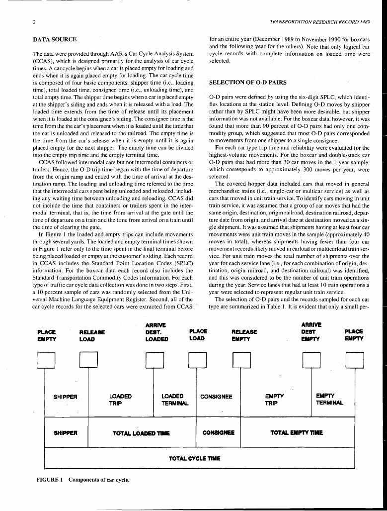
The data were provided through AAR's Car Cycle Analysis System (CCAS), which is designed primarily for the analysis of car cycle times. A car cycle begins when a car is placed empty for loading and ends when it is again placed empty for loading. The car cycle time is composed of four basic components: shipper time (i.e., loading time), total loaded time, consignee time (i.e., unloading time), and total empty time. The shipper time begins when a car is placed empty at the shipper's siding and ends when it is released with a load. The loaded time extends from the time of release until its placement when it is loaded at the consignee's siding. The consignee time is the time from the the car's placement when it is loaded until the time that the car is unloaded and released to the railroad. The empty time is the time from the car's release when it is empty until it is again placed empty for the next shipper. The empty time can be divided into the empty trip time and the empty terminal time.

CCAS followed intermodal cars but not intermodal containers or trailers. Hence, the 0-D trip time began with the time of departure from the origin ramp and ended with the time of arrival at the des­tination ramp. The loading and unloading time referred to the time that the intermodal cars spent being·unloaded and reloaded, includ­ing any waiting time between unloading and reloading. CCAS did not include the time that containers or trailers spent in the inter­modal terminal, that is, the time from arrival at the gate until the time of departure on a train and the time from arrival on a train until the time of clearing the gate.

In Figure 1 the loaded and empty trips can include movements through several yards. The loaded and empty terminal times shown in Figure 1 refer only to the time spent in the final terminal before being placed loaded or empty at the customer's siding. Each record in CCAS includes the Standard Point Location Codes (SPLC) information. For the boxcar data each record also includes the Standard Transportation Commodity Codes information. For each type of traffic car cycle data collection was done in two steps. First, a 10 percent sample of cars was randomly selected from the Uni­versal Machine Language Equipment Register. Second, all of the car cycle records for the selected cars were extracted from CCAS

TRANSPORTATION RESEARCH RECORD 1489

for an entire year (December 1989 to November 1990 for boxcars and the following year for the others). Note that only logical car cycle records with complete information on loaded time were selected.

SELECTION OF 0-D PAIRS

0-D pairs were defined by using the six-digit SP_LC, which identi­fies locations at the station level. Defining 0-D moves by shipper rather than by SPLC might have been more desirable, but shipper information was not available. For the boxcar data, however, it was found that more than 90 percent of 0-D pairs had only one com­modity group, which suggested that most 0-D pairs corresponded to movements from one shipper to a single consignee.

For each car type trip time and reliability were evaluated for the highest-volume movements. For the boxcar and double-stack car 0-D pairs that had more than 30 car moves in the 1-year sample, which corresponds to approximately 300 moves. per year, were selected.

The covered hopper data included cars that moved in general merchandise trains (i.e., single-car or multicar service) as well as cars that moved in unit train service. To identify cars moving in unit train service, it was assumed that a group of car moves that had the same origin, destination, origin railroad, destination railroad, depar­ture date from origin, and arrival date at destination moved as a sin­gle shipment. It was assumed that shipments having at least four car movements were unit train moves in the sample (approximately 40 moves in total), whereas shipments having fewer than four car movement records likely moved in carload or multicarload train ser­vice. For unit train moves the total number of shipments over the year for each service lane (i.e., for each combination of origin, des­tination, origin railroad, and destination railroad) was identified, and this was considered to be the number of unit train operations during the year. Service lanes that had at least 10 train operations a year were selected to represent regular unit train service.

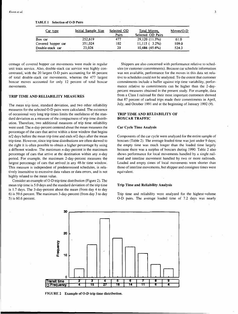
The selection of 0-D pairs and the records sampled for each car type are summarized in Table 1. It is evident that only a small per-

PLACE EMPTY

RELEASE LOAD

ARRIVE DEST. LOADED

PLACE LOAD

RF•FASE EMPTY

ARRIVE DEST EllPTY

Pl.ACE EMPTY

SHIPPER

SHIPPER

LOADED TRIP

LOADED TERMINAL

TOTAL LOADED T1IE

CONSIGNEE

CONSIGtEE

EMPTY TRIP

EMPTY TERMINAL

TOTAL EMPTY TIME

TOTAL CYCLE 1111E

FIGURE 1 Components of car cycle.

Kwon etal.

TABLE 1 Selection ofO-D Pairs

Car type Initial Sample Size

Box car Covered hopper car Double-stack car

252,619 351,024 23,026

centage of covered hopper car movements were made in regular unit train service. Also, double-stack car service was highly con­centrated," with the 20 largest 0-D pairs accounting for 46 percent of total double-stack car movements, whereas the 477 largest boxcar moves accounted for only 12 percent of total boxcar movements.

TRIP TIME AND RELIABILITY MEASURES

The mean trip time, standard deviation, and two other reliability measures for the selected 0-D pairs were calculated. The existence of occasional very long trip times limits the usefulness of the stan­dard deviation as a rrieasure of the compactness of trip time distrib­ution. Therefore, two additional measures of trip time reliability were used. The n-day-percent centered about the mean measures the percentage of the cars that arrive within a time window that begins n/2 days before the mean trip time and ends n/2 days after the mean trip time. However, since trip time distributions are often skewed to the right it is often possible to obtain a higher percentage by using a different window. The maximum n-day-percent is the maximum percentage of cars that arrive at the destination within any n-day period. For example, the maximum 2-day-percent measures the largest percentage of cars that arrived.in any 48-hr time window. This measure is independent of predetermined schedules, is rela­tively insensitive to excessive data values or data errors, and is not highly related to the mean value.

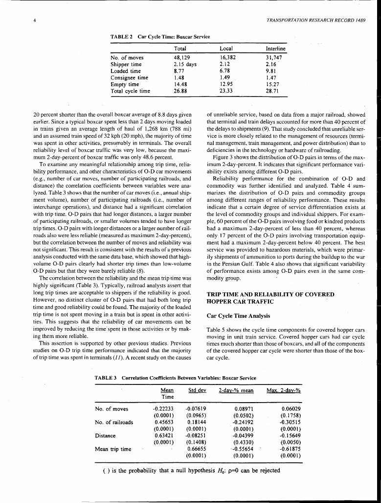
Consider an example of 0-D trip time distribution (Figure 2). The mean trip time is 5.0 days and the standard deviation of the trip time is 1.7 days. The 3-day-percent about the mean (from day 4 to day 6) is 59.6 percent. The maximum 3-day-percent (from day 3 to day 5) is 60.6 percent.

20

()' c CD ;::,

l ,.

10

Selected OD Pairs 477 102 20

Total Moves. Selected OD Pairs

29,120 (11.5%) 11,115 ( 3.2%) 10,486 (45.6%)

Moves/0-D

61.0 109.0 524.3

3

Shippers are also concerned with performance relative to sched­ules (or customer commitments). Because car schedule information was not available, performance for the moves in this data set rela­tive to schedules could not be analyzed. To the extent that customer commitments include a buffer against trip time variability, perfor­mance relative to commitments can be higher than the 2-day­percent measures obtained in the present study. For example, data from a Class I railroad for their most important customers showed that 87 percent of carload trips made their commitments in April, July, and October 1991 and at the beginning of January 1992 (9).

TRIP TIME AND RELIABILITY OF B'oxCAR TRAFFIC

Car Cycle Time Analysis

Components of the car cycle were analyzed for the entire sample of boxcars (Table 2). The average loaded time was just under 9 days; the empty time was much longer than the loaded time largely because there was a surplus of boxcars during 1990. Table 2 also shows performance for local movements handled by a single rail­road and interline movement handled by two or more railroads. Loaded and empty times of local movements were shorter than those of interline movements, but shipper and consignee times were equivalent.

Trip Time and Reliability Analysis

Trip time and reliability were analyzed for the highest-volume 0-D pairs. The average loaded time of 7.2 days was nearly

3 I ;, I 14 !Transit time I 15

5 6 18

FIGURE 2 Example of 0-D trip time distribution.

4 TRANSPORTATION RESEARCH RECORD 1489

TABLE2 Car Cycle Time: Boxcar Service

Total

No. of moves 48, 129 Shipper time 2.15 days Loaded time 8.77 Consignee time l.48 Empty time 14.48 Total cycle time 26.88

20 percent shorter than the overall boxcar average of 8.8 days given earlier. Since a typical boxcar spent less than 2 days moving loaded in trains given an average length of haul of 1,268 km (788 mi) and an assumed train speed of 32 kph (20 mph), the majority of time was spent in other activities, presumably in terminals. The overall reliability level of boxcar traffic was very low, because the maxi­mum 2-day-percent of boxcar traffic was only 48.6 percent.

To examine any meaningful relationship among trip time, relia­bility performance, and other characteristics of 0-D car movements (e.g., number of car moves, number of participating railroads, and distance) the correlation coefficients between variables were ana­lyzed. Table 3 shows that the number of car moves (i.e., annual ship­ment volume), number of participating railroads (i.e., number of interchange operations), and distance had a significant correlation with trip time. 0-D pairs that had longer distances, a larger number of participating railroads, or smaller volumes tended to have longer trip times. 0-D pairs with longer distances or a larger number of rail­roads also were less reliable (measured as maximum 2-day-percent), but the correlation between the number of moves and reliability was not significant This result is consistent with the results of a previous analysis conducted with the same data base, which showed that high­volume 0-D pairs clearly had shorter trip times than low-volume 0-D pairs but that they were barely reliable (8).

The correlation between the reliability and the mean trip time was highly significant (Table 3). Typically, railroad analysts assert that long trip times are acceptable to shippers if the reliability is good. However, no distinct cluster of 0-D pairs that had both long trip time and good reliability could be found. The majority of the loaded trip time is not spent moving in a train but is spent in other activi­ties. This suggests that the reliability of car movements can be improved by reducing the time.spent in those activities or by mak­ing them more reliable.

This assertion is supported by other previous studies. Previous studies on 0-D trip time performance indicated that the majority of trip time was spent in terminals (11). A recent study on the causes

Local Interline

16,382 31, 747 2.12 2.16 6.78 9.81 l.49 l.47 12.95 15.27 23.33 28.71

of unreliable service, based on data from a major railroad, showed that terminal and train delays accounted for more than 40 percent of the delays to shipments (9). That study concluded that unreliable ser­vice is more closely related to the management of resources (termi­nal management, train management, and power distribution) than to deficiencies in the technology or hardware of railroading.

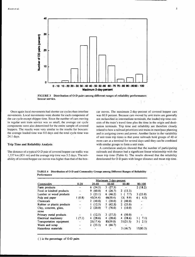
Figure 3 shows the distribution of 0-D pairs in terms of the max­imum 2-day-percent. It indicates that significant performance vari­ability exists among different 0-D pairs.

Reliability performance for the combination of 0-D and commodity was further identified and analyzed. Table 4 sum­marizes the distribution of 0-D pairs and commodity groups among different ranges of reliability performance. These results indicate that a certain degree of service differentiation exists at the level of commodity groups and individual shippers. For exam­ple, 60 percent of the 0-D pairs involving food or kindred products had a maximum 2-day-percent of less than 40 percent, whereas only 17 percent of the 0-D pairs involving transportation ·equip­ment had a maximum 2-day-percent below 40 percent. The best service was provided to hazardous materials, which were primar­ily shipments of ammunition to ports during the buildup to the war in the Persian Gulf. Table 4.also shows that significant variability of performance exists ·among 0-D pairs even in the same com­modity group.

TRIP TIME AND RELIABILITY OF COVERED HOPPER CAR TRAFFIC

Car Cycle Time Analysis

Table 5 shows the cycle time components for covered hopper cars moving in unit train service. Covered hopper cars had car cycle times much shorter than those of boxcars, and all of the components of the covered hopper car cycle were shorter than those of the box­car cycle.

TABLE 3 Correlation Coefficients Between Variables: Boxcar Service

Mean Std dev 2-da:r:-% mean Max. 2-da~-% Time

No. of moves -0.22233 -0.07619 0.08971 0.06029 (0.0001) (0.0965) (0.0502) (0.1758)

No. of railroads 0.45653 0.18144 -0.24192 -0.30515 (0.0001) (0.0001) (0.0001) (0.0001)

Distance 0.63421 -0.08251 -0.04399 -0.15649 (0.0001) (0.1408) (0.4330) (0.0050)

Mean trip time 0.66655 -0.55654 -0.61875 (0.0001) . (0.0001) (0.0001)

( ) is the probability that a null hypothesis H0 : p=O can be rejected

Kwon eta/.

I 30

-t! l 20 c 0 '?;

~ § 10 z

5

0-10 10-20 20-30 30.40 40.50 so-eo eo-70 70-80 ao-eoeo-100 Maximum 2-<tay-percent

FIGURE 3 Distribution of 0-D pairs among different ranges of reliability performance: boxcar service.

Once again local movements had shorter car cycles than interline movements. Local movements were shorter for each component of the car cycle except shipper time. Since the number of cars moving in regular unit train service was so small, the average car cycle components were also determined for the entire sample of covered hoppers. The results were very similar to the results for boxcars: the average loaded time was 9.0 days and the total cycle time was 24.l days.

Trip Time and Reliability Analysis

The distance of a typical 0-D pair of covered hopper car traffic was 1,337 km (831 mi) and the average trip time was 5.2 days. The reli­ability of covered hopper car moves was higher than that of the box-

car moves. The maximum 2-day-percent of covered hopper cars was 60.9 percent. Because cars moved by unit trains are generally not reclassified in intermediate terminals, the loaded trip time con­sists of the train's travel time plus the time in the origin and desti­nation terminals. Trip time and reliability are therefore closely related to how a railroad prioritizes unit trains in meet/pass planning and in assigning crews and power. Another factor in the variability of unit train trip times is that some railroads hold groups of. 40 or more cars at a terminal for several days until they can be combined with similar groups to form a unit train.

A correlation analysis showed that the number of participating railroads and distance had a significant linear relationship with the mean trip time (Table 6). The results showed that the reliability deteriorated for 0-D pairs with longer distance and mean trip time.

TABLE4 Distribution of 0-D and Commodity Groups among Different Ranges of Reliability Performance

Maximum 2-da:z::-~ercent Commodi~ 0-20 20-40 40-60 60-80 80-100 Fann products 6 (54.5) 3 (27.3) 2 (18.2) Food or kindred products 9 (60.0) 4 (26.7) 2 (13.3) Lumber or wood products 3 (23. l) 6 (46.2) l ( 7.7) 3 (23.0) Pulp and paper l (0.8) 45(34.4) 66(50.4) 13( 9.9) 6 ( 4.5) Chemicals 2 (40.0) 1 (20.0) 2 (40.0) Rubber or plastic products l (12.5) 5 (62.S) 2 (25.0) Clay, concrete, glass, 2 (20.0) 7 (70.0) 1 (10.0) stone Primary metal products (12.5) 3 (37.5) 4 (50.0) Electrical machinery 1 (7.1) 4 (28.6) 4 (28.6) 4 (28.6) 1 ( 7.1) Transportation equipment 25(17.4) 85(59.0) 31(21.5) 3 ( 2.1) Waste and scrap 2 (33.3) 4 (66.7) Hazardous materials 3 (16.7) 15(83.3)

( ) is the percentage of 0-D pairs

6 TRANSPORTATION RESEARCH RECORD 1489

TABLE 5 Car Cycle Time: Covered Hopper Car Service

No. of moves Shipper time Loaded time Consignee time Empty time Total cycle time

Total

6,799 1.92 days 5.33 . 1.27 6.76 15.27

The correlations between the number of car moves or the number of railroads and reliability were not significant. The correlation between the reliability and the mean trip time was again highly sig­nificant. In fact, covered hopper car service had an even stronger linear relationship between the reliability and the mean 'trip time (p = -0.77 versus -0.62 for the boxcar service).

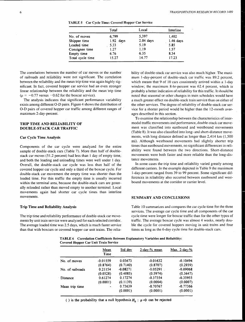
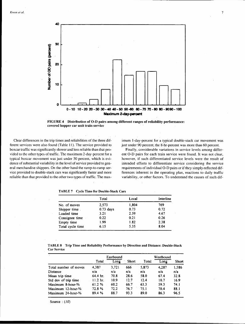
The analysis indicates that significant performance variability exists among different 0-D pairs. Figure 4 shows the distribution of 0-D pairs of covered hopper car traffic among different ranges of · maximum 2-day-percent.

TRIP TIME AND RELIABILITY OF DOUBLE-STACK CAR TRAFFIC

Car Cycle Time Analysis

Components of the car cycle were analyzed · for the entire sample of double-stack cars (Table 7). More than half of double­stack car moves (5 I .2 percent) had less than 1 day of empty time; and both the loading and unloading times were wen under I day. Overall, the double-stack car cycle was less than half of the covered hopper car cycle and only a third of the boxcar cycle. For double-stack car movement the empty time was shorter than the loaded time. For this traffic the empty time is usually incurred within the terminal area, because the double-stack cars are gener­ally reloaded rather than moved empty to another terminal. Local movements again had shorter car cycle times than interline movements.

Trip Time and Reliability Analysis

The trip time and reliability performance of double-stack car move­ments by unit train service were analyzed for each selected corridor. The average loaded time was 2.5 days, which is much faster service than that with boxcars or covered hopper car unit trains. The relia-

Local

5,397 2.04 days 5.19 1.19 6.35 14.77

Interline

1,402 1.46 days 5.85 1.57 8.34 17.23

bility of double-stack car service was also much higher. The maxi­mum I-day-percent of double-stack car traffic was 89 .2 percent, which means that 9 of 10 cars consistently arrived within a I-day window; the maximum 8-hr-percent was 62.4 percent, which is probably a better indication of reliability for this traffic. It should be noted that seasonal or other changes in train schedules would have a much greater effect on double-stack train service than on either of the other services. The degree of reliability of double-stack car ser­vice for a shorter period would be higher than the I 2-month aver­ages described in this section.

To examine the relationship between the characteristics of inter­modal traffic movements and performance, double-stack car move­ment was classified into eastbound and westbound movements (Table 8). It was also classified into long- and short-distance move­ments, with long distance defined as longer than 2,4I4 km (1,500 mi). Although westbound movements had slightly shorter trip times than eastbound movements, no significant differences in reli­ability were found between the two directions. Short-distance movements were both faster and more reliable than the long-dis­tance movements.

In some cases the trip time and reliability varied greatly among different carriers. In the example depicted in Table 9 the maximum I-day-percent ranged from 39 to 99 percent. Some significant dif­ferences in reliability also occurred between eastbound and west­bound movements at the corridor or carrier level.

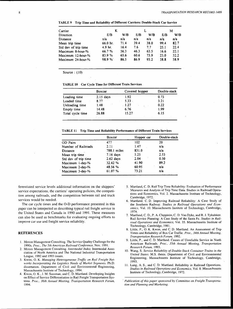
SUMMARY AND CONCLUSIONS

Table I 0 summarizes and compares the car cycle time for the three services. The average car cycle time and all components of the car cycle time were longer for boxcar traffic than for the other types of traffic. The average boxcar cycle was almost 4 weeks, nearly dou­ble the cycle for covered hoppers moving in unit trains and four times as long as the 6-day cycle time for double-stack cars.

TABLE 6 Correlation Coefficients Between Explanatory Variables and Reliability: Covered Hopper Car Unit Train Service

Mean Std dev 2-day-% mean Max. 2-day-% Time

No. of moves -0.01559 0.03673 -0.01632 -0.10494 (0.8764) (0.7140) (0.8707) (0.2939)

No. of railroads 0.21154 -0.08271 -0.05291 -0.09068 (0.0328) (0.4085) (0.5974) (0.3647)

· Distance 0.61274 0.17274 -0.37354 -0.35955 (0.0001) (0.1139) (0.0004) (0.0007)

Mean trip time 0.73639 -0.70767 -0.77366 (0.0001) (0.0001) (0.0001)

( ) is the probability that a null hypothesis H0 : p==O can be rejected

Kwon et al. 7

I so

(!

l 20

8 'S

.! § 10 z

0-10 10-20 20-30 30-40 40.50 50-80 80-70 70-80 80-9090-100 Maximum 2-day-percant

FIGURE 4 Distribution of 0-D pairs among different ranges of reliability performance: covered hopper car unit train service

Clear differences in the trip times and reliabilities of the three dif­ferent services were also found (Table 11). The service provided to boxcar traffic was significantly slower and less reliable than that pro­vided to the other types of traffic. The maximum 2-day-percent for a typical boxcar movement was just under 50 percent, which is evi­dence of substantial variability in the level of service provided to gen­eral merchandise shippers. On the other hand the ramp-to-ramp ser­vice provided to double-stack cars was significantly faster and more reliable than that provided to the other two types of traffic. The max-

imum 1-day-percent for a typical double-stack car movement was just under 90 percent; the 8.,.hr-percent was more than 60 percent.

Finally, considerable variations in service levels among differ­ent 0-D pairs for each train service were found. It was not clear, however, if such differentiated service levels were the result of intended efforts to differentiate service considering the service requirements of individual 0-D pairs or if they simply-reflected dif­ferences inherent in the operating plan, reactions to daily traffic variability, or other factors. To understand the causes of such dif-

TABLE 7 Cycle Time for Double-Stack Cars

Total Local Interline

No. of moves 2,573 1,804 769 Shipper time 0.73 days 0.73 0.72 Loaded time 3.21 2.59 4.67 Consignee time 0.22 0.21 0.26 Empty time 1.99 1.82 2.38 Total cycle time 6.15 5.35. 8.04

TABLES Trip Time and Reliability Performance by Direction and Distance: Double-Stack Car Service

Eastbound Westbound Total Lona Short Total Lon~ Short

Total number of moves 4,387 3,721 666 5,873 4,287 1,586 Distance n/a n/a n/a n/a n/a n/a Mean trip time 64.4 hr. 70.8 28.6 58.0 67.4 32.8 Std dev of trip time 11.2 hr. 10.9 12:7 12.4 10.7 16.9 Maximum 8-hour-% 61.2 % 60.2 66.7 63.3 59.3 74.1 Maximum 12-hour-% 72.8 % 72.2 76.7 75.1 70.4 88.1 Maximum 24-hour-% 89.4 % 88.7 93.3 89.0 86.3 96.5

Source : ( J 0)

8 TRANSPORTATION RESEARCH RECORD 1489

TABLE 9 Trip Time and Reliability of l)ifferent Carriers: Double-Stack Car Service

Carrier K L M Direction EIB WIB E/B WIB E/B W/B Distance n/a n/a n/a n/a n/a n/a Mean trip time 66.0 hr. 71.4 39.4 38.0 99.4 82.7 Std dev of trip time 4.9 hr. 16.4 7.6 7.7 25. l 22.4 Maximum 8-hour-% 66.7 % 56.3 46.3 63.5 16.6 22.l Maximum 12-hour-% 83.9 % 65.6 60.6 73.9 23.0 32.2 Maximum 24-hour-% 98.9 %" 86.5 86.9 93.2 38.8 58.9

Source : ( 10)

TABLE 10 Car Cycle Time for Different Train Services

Boxcar Covered hopper Double-stack

Loading time 2.15 days 1.92 0.73 Loaded time 8.77 5.33 . 3.21 Unloading time 1.48 1.27 0.22 Empty time 14.48 6.76 1.99 Total cycle time 26.88 15.27 6.15

TABLE 11 Trip Time and Reliability Performance of Different Train Services

Boxcar Hopper car Double-stack

OD Pairs 477 102 20 Number of Railroads 2.11 1.47 n/a Distance 788.l miles 831.0 n/a Mean trip time 7.16 days Std dev of trip time 2.62 days Maximum 1-day-% 32.42 % Maximum 2-day-% 48.56 % Maximum 3-day-% 61.07 %

ferentiated service levels additional information on the shippers' service expectations, the carriers' operating policies, the competi­tion among railroads, and the competition between rail and truck services would be needed.

The car cycle times and the 0-D performance presented in this paper can be interpreted as describing typical rail freight service in the United States and Canada in I 990 and 1991. These measures can also be used as benchmarks for evaluating ongoing efforts to improve car use and freight service reliability.

REFERENCES

I. Mercer Management Consulting. The Service Quality Challenge for the 1990s. Proc., The 5th American Railroad Conference, Nov. 1991.

2. Mercer Management Consulting. Intermodal Index_. Intermodal Asso­ciation of North America and The National Industrial Transportation League, 1992 and 1993 issues.

3. Kwon, 0. K. Managing Heterogeneous Traffic on Rail Freight Net­works Incorporating the Logistics Needs of Market Segments. Ph.D. dissertation. Department of Civil and Environmental Engineering, Massachusetts Institute of Technology, 1994.

4. Kwon, 0. K., J.M. Sussman, and C. D. Martland. Developing Insights on Effect of Service Differentiation in Rail Freight Transportation Sys­tems. Proc., 36th Annual Meeting, Transportation Research Forum, 1994.

5.25 2.53 2.04 0.50 41.90 89.2 60.95 n/a 73.21 n/a

5. Martland, C. D. Rail Trip Time Reliability: Evaluation of Performance Measures and Analysis of Trip Time Data. Studies in Railroad Opera­tions and Economics, Vol. 2. Massachusetts Institute of Technology, Cambridge, 1972.

6. Martland, C. D. Improving Railroad Reliability: A Case Study of the Southern Railway. Studies in Railroad Operations and Econ­omics, Vol. 10. Massachusetts Institute of Technology, Cambridge, 1974.

7. Martland, C. D., P.A. Clappison, C. D. Van Dyke, and R. J. Tykulsker. Rail Service Planning: A Case Study of the Santa Fe. Studies in Rail­road Operations and Economics, Vol. 35. Massachusetts Institute of Technology, Cambridge, 1981.

8. Little, P., 0. K. Kwon, and C. D. Martland. An Assessment of Trip Times and Reliability of Box Car Traffic. Proc., 34th Annual Meeting, Transportation Research Forum, 1992.

9. Little, P., and C. D. Martland. Causes of Unreliable Service in North American Railroads. Proc., 35th Annual Meeting, Transportation Research Forum, 1993.

IO. Wang, S. Service Reliability of Double-Stack Container Trains in the United States. M.S. thesis. Department of Civil and Environmental Engineering, Massachusetts Institute of Technology, Cambridge, 1993.

11. Lang, A. S., and C. D. Martland. Reliability in Railroad Operations. Studies in Railroad Operations and Economics, Vol. 8. Massachusetts Institute of Technology, Cambridge, 1972.

· Publication of this paper sponsored by Committee on Freight Transporta­tion and Planning and Marketing.

TRANSPORTATION RESEARCH RECORD 1489 9

Modeling Single-Line Train Operations

A. HIGGINS, L. FERREiRA, AND E. KOZAN

Scheduling of trains on a single line involves the use of train priorities for the resolution of conflicts. First, a mathematical programming model is described. The model schedules trains over a single line of track when the priority of each train in a conflict depends on an estimate of the remaining crossing and overtaking delay. This priority is used in a branch-and-bound procedure to allow the determination of optimal solutions quickly. This is demonstrated with the use of an example. Rail operations over a single-line track require the existence of a set of sid­ings at which trains can cross or overtake each other. Investment deci­sions on upgrading the numbers and locations of these sidings can have a significant impact on both customer service and rail profitability. Sid­ings located at insufficient positions may lead to high operating costs and congestion. Second, a model to determine the optimal position of a set of sidings on a single-track rail corridor is described. The sidings are positioned to minimize the total delay and train operating costs of a given cyclic train schedule. The key feature of the model is the allowance of nonconstant train _velocities and nonuniform departure times.

This paper deals with two problems of single-line train scheduling, namely, the on-line scheduling of trains over a single-line track with multiple sidings and the optimum location of the sidings with respect to a given schedule. Part! deals with the optimum dis­patching of trains on a single line of track. Trains can be dispatched from either end or from intermediate points on the track. When two trains approach each other on a single line one of them must take the siding for the safe operation of the system. Determining which train takes the siding is done by taking into account such factors as train priority, distance, lateness, and train operating costs. It is com­mon practice for train operators to set a fixed timetable through which conflicts are resolved. A train dispatcher in a control center will act in the event of unforseen events. Because these events can cause delays to trains the dispatcher needs to continually alter the given timetable and resolve new conflicts. This is usually performed manually under strict time constraints so that the number of alter­natives that can be assessed is very limited.

The operator's experience and knowledge of local conditions will continue to be used. Train dispatching decisions, which to a certain extent involve human as well as technical factors, will require human intervention to resolve problems. However, with the avail­ability of such an optimization model, the operator is able to quickly update a schedu_le as unplanned events occur. The new optimal schedule offered by the model may not be fully implementable for practical reasons. However, the gap between the optimum and the practically feasible schedule can readily be assessed. The penalty for not being able to implement the optimum schedule in terms of operating cost and travel time reliability can be evaluated against the practical factors that prevent implementation of the optimum schedule.

A. Higgins and E. Kozan, School of Mathematics, Queensland University of Technology, P.O. Box 2434, QLD 4001, Australia. L. Ferreira, School of Civil Engineering, Queensland University of Technology, P.O. Box 2434, QLD 400 I, Australia.

With the on-line train scheduling problem the determination of the priority of a train at a particular point on the journey involves the consideration of the initial priority, current lateness of the train, and a lower-bound estimate of possible further conflict delay. Exploiting such a lower bound in a model will act as a look-ahead function and will allow optimum schedules to be located quickly.

A second major use of the model relates to the planning of rail­road operations. Such planning can be conveniently divided into two components, namely, short- to medium-term train planning and railroad infrastructure planning associated with train operations. The model can be used to evaluate the implications of changes to a timetable in terms of changed train departures, additional trains, and changes in train speeds. The optimum scheduling algorithm can be used as a simulator of proposed changes. Finally, the model can be used for long-range planning of railroad operations. In Australia, two main infrastructure planning issues are under investigation, namely, the upgrading of main line track to allow higher speeds and heavier axle loads and the need to extend sidings to allow for longer trains. The scheduling optimization model can be used to evaluate both of these investment strategies. The impact on the schedule of extending some sidings and not others can be assessed by using the model to simulate the effects of the proposed changes on future schedules. The removal of sidings has a cost in terms of flexibility and feasibility of schedules.

Part II deals with the development of a model for estimating the optimum positions of sidings on a single line of track. With high capital costs a rail line must be designed as economically as possi­ble, and at the same time it must have enough capacity to accom­modate the forecast demand. Planning for a rail line involves deter­mining the number of sidings required, the length of each siding, its position, and the vertical and horizontal alignments for the line.

When determining the positions of sidings several variables must be considered. The sidings must be placed in order to minimize train delays and total train operating costs. If too many sidings are planned for the initial capital costs will outweigh the long-term ben­efits and there will be wasted capacity.

PART I: OPTIMUM TRAIN SCHEDULES

Past Research

Research involving the scheduling of trains on a single line of track is extensive, and the following highlights the major developments.

Kraft (1) developed a dispatching rule giving the optimal time advantage for a particular train based on train priority, track running times, and the delay penalties of each train. A similar method dis­cussed by Sauder and Westerman (2) was implemented as a Deci­sion Support System in a railway division of the United States. Those models, which assume fixed train speeds, produce train plans that minimize the weighted total travel times.

10

Kraay et al. (3) were the first to look at the idea of determining the cross-overtake plan and velocity profile to pace trains to con­serve fuel while keeping the lateness of the trains to a minimum. Formulated constraints similar to those of Kraay et al. (3) were used in an interactive Decision Support System (SCAN) by Jovanovic and Harker ( 4) to develop reliable train schedules by using current schedules. Mills et al. (5) formulated a discrete network-type model by discretizing the departure and arrival time variables of this for­mulation.

Model Formulation

Assumptions and Inputs

The foliowing assumptions are made with regard to the model in this section:

• The track is divided into segments that are separated by sid­ings.

• Crossing and overtaking can occur at any siding or double-line track segments.

• Trains can follow each other on a track segment with a mini­mum headway.

• For double-line track sections it is assumed that one lane will be allocated for inbound trains and one lane will be allocated for outbound trains. Usually, signal points will be set up this way.

• Scheduled stops are permitted at any intermediate siding for any train.

The model will require various pieces of information as inputs to the model. The specific information is as follows:

• An unresolved train plan to make available the number of over­take and cross interferences for each train.

• The initial priorities of each train. These are determined by several· factors such as the type of train, customer contract agree­ments, and train load.

• The upper and lower velocity limits for each train (which are dependent on the physical characteristics of the track segment and the train).

• Segment lengths and the identifiqttion of single- and double­line track segments.

• The times of any scheduled train stops. These stops may include those for loading and unloading, refueling, and crew changes.

Definition of Variables

The set of trains is denoted by I= {I, 2, ... , m, m + 1, ... n} for which inbound trains are from 1 to m and outbound trains are from m + 1 ton. The variables used in the model are listed and described in this section.

where P, is equal to a set of single-line tracks and P 2 is equal to a set of double-line tracks. The integer decision variables for deter­mining which train traverses a section first (and which also deter­mines the position of conflict resolution) are given by the fol­lowing:

TRANSPORTATION RESEARCH RECORD 1489

{

I if inbound train i ::; m traverses track segment p E P 1

A;1p = before inbound train}::; m 0 otherwise

{

1 if inbound train i::; m traverses track segment p E P 1

B;1p = before outbound train j > m 0 otherwise

{

1 if outbound train i > m traverses track segment p E P 1

cijp = before outbound train}> m 0 otherwise

The arrival and departure time decision variables are as follows:

X~q = arrival time of train i E I at station q E Q, X~q = departure time of train i E I from station q E Q, Xb; = departure time of train i E I from its origin station, and Xb; = arrival time of train i E I at its destination station.

The input parameters are defined as follows:

hp= minimum headway between two trains on segmentp E Pi. dP = length of segment p E P, Y~; = planned departure time of train i E I from origin station, YJ; = planned arrival time of train i E I at destination station, y_j, = minimum allowable velocity of train i E I on segment

pEP, Vj,= maximum achievable average velocity of train i E I on

segment p E P,

W; = initial priority of train i E I (highest for passenger trains), and

S~ = scheduled stop time for train i E I at station q E Q.

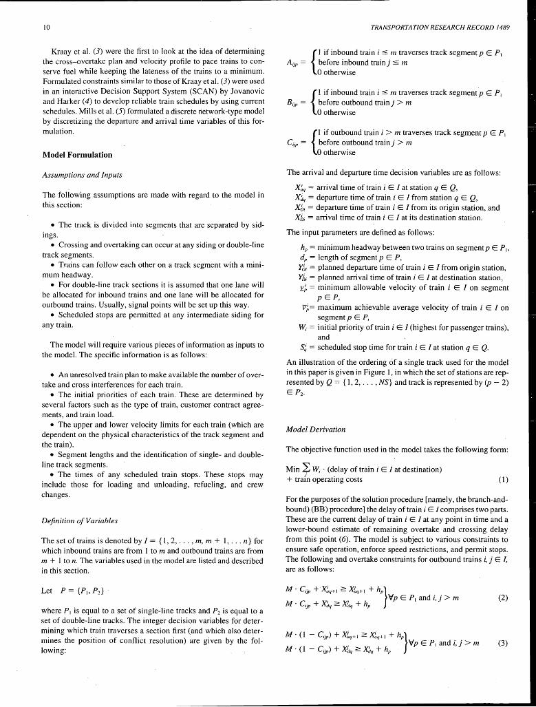
An illustration of the ordering of a single track used for the model in this paper is given in Figure 1, in which the set of stations are rep­resented by Q = { 1, 2, ... , NS} and track is represented by (p - 2) E Pz.

Model Derivation

The objective function used in the model takes the following form:

Min~ W; · (delay of train i E I at destination) + train operating costs (1)

For the purposes of the solution procedure [namely, the branch-and­bound) (BB) procedure] the delay of train i EI comprises two parts. These are the current delay of train i E I at any point in time and a lower-bound estimate of remaining overtake and crossing delay from this point (6). The model is subject to various constraints to ensure safe operation, enforce speed restrictions, and permit stops. The following and overtake constraints for outbound trains i, j E /, are as follows:

(2)

(3)

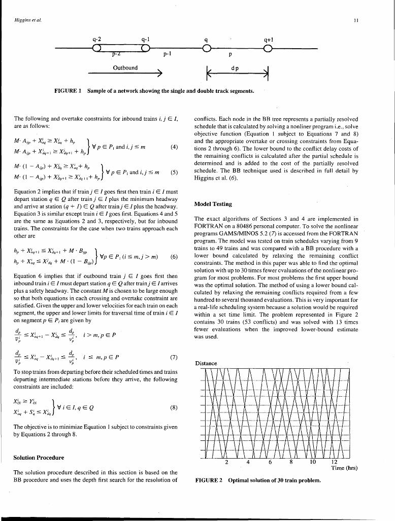
Higgins et al. 11

q-2 q-1 q q+l

() () 0 0 p-2 p-1 p

Outbound ) ~

dp

~ FIGURE 1 Sample of a network showing the single and double track segments.

The following and overtake constraints for inbound trains i, j E /, are as follows:

(4)

(5)

Equation 2 implies that if train) E I goes first then train i EI must depart station q E Q after train j E I plus the minimum headway and arrive at station (q + J)·E Q after train) E 1 plus the headway. Equation 3 is similar except train i E I goes first. Equations 4 and 5 are the same as Equations 2 and 3, respectively, but for inbound trains. The constraints for the case when two trains approach each other are

(6)

Equation 6 implies that if outbound train j E I goes first then inbound train i EI must depart station q E Q after train) EI arrives plus a safety headway. The constant Mis chosen to be large enough so that both equations in each crossing and overtake constraint are satisfied. Given the upper and lower velocities for each train on each segment, the upper and lower limits for ti-aversal time of train i E I on segment p E P1 are given by

dP <Xi . dP -i - aq+ I - Xdq :::;; ---:- , i > 111, P E P VP V~

dP < Xi - X; < dP - . - aq dq+ I - . ' i :::;; m, p E p v~ ~

(7)

To stop trains from departing before their scheduled times and trains departing intermediate stations before they arrive, the following constraints are included:

(8)

The objective is to minimize Equation I subject to constraints given by Equations 2 through 8.

Solution Procedure

The solution procedure described in this section is based on the BB procedure and uses the depth first search for the resolution of

conflicts. Each node in the BB tree represents a partially resolved schedule that is calculated by solving a nonliner program i.e., solve objective function (Equation 1 subject to Equations 7 and 8) and the appropriate overtake or crossing constraints from Equa­tions 2 through 6). The lower bound to the conflict delay costs of the remaining conflicts is calculated after the partial schedule is determined and is added to the cost of the partially resolved schedule. The BB technique used is described in full detail by Higgins et al. (6).

Model Testing

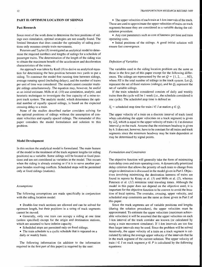
The exact algorithms of Sections 3 and 4 are implemented in FORTRAN on a 80486 personal computer. To solve the nonlinear programs GAMS/MINOS 5.2 (7) is accessed from the FORTRAN program. The model was tested on train schedules varying from 9 trains to 49 trains and was compared with a BB procedure with a lower bound calculated by relaxing the remaining conflict constraints. The method in this paper was able to find the·optimal solution with up to 30 times fewer evaluations of the nonlinear pro­gram for most problems. For most problems the first upper bound was the optimal solution. The method of using a lower bound cal­culated by relaxing the remaining conflicts required from a few hundred to several thousand evaluations. This is very important for a real-life scheduling system because a solution would be required within a set time limit. The problem represented in Figure 2 contains 30 trains (53 conflicts) and was solved with 13 times fewer evaluations when the improved lower-bound estimate was used.

Distance

4 6 8 10 12 Time (hrs)

FIGURE 2 Optimal solution of 30 train problem.

12

PART II: OPTIMUM LOCATION OF SIDINGS

Past Research

Since most of the work done to determine the best positions of sid­ings uses simulation, optimal strategies are not usually found. The limited literature that does consider the optimality of siding posi­tions only assumes simple train movements.

Petersen and Taylor (8) investigated an analytical model to deter­mine the required numbers and lengths of sidings for a schedule of passenger trains. The determination of the length of the siding was to obtain the maximum benefit of the acceleration and deceleration characteristics of the trains.

An approach was taken by Kraft (9) to derive an analytical equa­tion for determining the best position between two yards to put a siding. To construct the model free running time between sidings, average running speed (including delays), and the number of trains per unit of time was considered. The model cannot consider multi­ple sidings simultaneously. The equation may, however, be useful as an initial estimate. Mills et al. (10) use simulation, analytic, and heuristic techniques to investigate the line capacity of a mine-to­port track system. The analytic model, which determines the opti­mal number of equally spaced sidings, is based on the expected crossing delay to a train.

None of the studies described earlier considers solving for the optimal positions of sidings without the assumption of con­stant velocities and equally spaced sidings. The remainder of this paper considers the model formulation and solution to this problem.

Model Development

In this section the analytical model is formulated. The main feature of the model is the treatment of the track segment lengths (or siding positions) as a variable. Some sidings will be located at fixed posi­tions and are not considered as variables in the model. This occurs when the siding is already existing or if it is to serve another pur­pose besides resolving conflicts. Scheduled stops will be permitted only at fixed sidings (stations).

Assumptions

The following assumptions are made specifically in conjunction with the siding location model:

• Double-line track sections are allowed and can be solved for optimum length, but their positions in a string of track segments cannot be moved.

• Generally, only one train can occupy a siding at one time (unless specified) except for the origin and destination stations, which are assumed to have infinite capacity.

• Scheduled stops are permitted only on fixed sidings. • The train schedule is a cyclic schedule that is repeated on a daily or weekly basis.

The following information (in addition to the information required in the first part of this paper) is required by the user:

TRANSPORTATION RESEARCH RECORD 1489

• The upper velocities of each train at 1-km intervals of the track. These are usedto approximate the upper velocities of trains on track segments because they are considered as a variable during the cal­culation procedure.

• Any cost parameters such as cost of lateness per time and train operating costs.

• Initial positions of the sidings. A good initial solution will ensure fast convergence.

Definition of Variables

The variables used in the siding location problem are the same as those in the first part of this paper except for the following differ­ences. The sidings are represented by the set Q = { 1, 2, ... , NS}, where NS is the total number of sidings in the track system. Let Q 1

represent the set of fixed stations (sidings), and let Q2 represent the set of variable sidings.

If the train schedule considered consists of daily and weekly trains then the cycle will be 1 week (i.e., the schedule considered is one cycle). The scheduled stop time is defined as

S~ = scheduled stop time for train i"E I at station q E Q1

The upper velocity of a train on a discrete interval of track (used when calculating the upper velocities on a track segment) is given by veli, which is equal to the upper velocity of train i E I at distance interval g on the track. Assume that the minimum headway is given by h. It does not, however, have to be constant for all trains and track segments since the minimum headway may be train dependent or may be determined by signal points.

Formulation and Constraints

The objective function will generally take the form of minimizing train delay costs and train operating costs. A dynamically prioritized delay criterion that allows the priority of each train to change from origin to destination is discussed in the model given in Part I. Objec­tives involving minimizing the destination lateness of trains are found in reports by Kraay et al. (3) and Mills et al. (5), whereas Petersen et al. (l J) minimize total traveling times. Although the model in this paper does not depend on the objective used, it is important for the objective function to be convex to avoid the loca­tion of local optima. The overtake, crossing, upper velocity, and scheduled stop constraints are the same as those given in Part I of this paper.

Since the track segments are of variable positions and lengths (during the solution procedure), the upper velocities must be approximated. To estimate the upper velocities (maximum achiev­able velocities) it will be assumed that the upper velocities on each 1-km interval of the track corridor are known (or calculated by using a train movement simulator). If 1-km intervals are too fine then larger intervals may be used. Since the problem will be solved iteratively, the upper velocity of a train on a track segment is cal­culated by taking the average upper velocity of the intervals that lie in the track segment of the current solution. The upper velocity of train i E I on track segment p E P is calculated by the following equations:

Higgins et al.

dh

I;;i~ g =di

v~=-----(dh - di)+ 1 (9)

where di is equal to the integer part of ( 'f d,) + 1, and dh is equal to the integer part of ct. d,) k= I

The expected arrival times at intermediate sidings are also depen­dent on the positions of sidings and are calculated by first deter­mining the planned velocities on the track segments. The planned velocities are calculated as follows:

RA;=----L 1. 8 vel;

where RA; is the ratio of the fastest journey time to the expected journey time, and

where PV/, is the planned velocity of train i E I on track segment p E P. From the planned velocity the expected departures from each of the intermediate stations are calculated by using Equation 10. The expected arrival times will be the same as the expected depar­ture times unless there are scheduled stops.

. . q~I dk . . I . b d Yriq = Ya; + L --. , tram 1 E Is out oun

k=I PVk

. . ~ dk . . /' .: b d Yriq = Yo; + L --. , tram 1 E IS m oun k=q PVk

(10)

where TRP is the number of track segments on the rail corridor. The fastest times that the trains travel from origin to destination are assumed to not be affected by the siding positions, so the expected · arrivals and departures at these sidings do not change. The last con­straint is to ensure that the sum of the length of the track segments is equal to the length of the entire track corridor, that is

i-1

Ldk = TLEN;, i E Q, k=I

(11)

where TLEN; is the length of the track system from the origin to the fixed siding i E Q1•

Solving the Model

In this section a decomposition procedure is presented to obtain a solution to the formulation presented earlier. Solving the problem as formulated can be difficult because of the requirement that three sets of variables be solved (track segment lengths, arrival and depar­ture times, and binary conflict resolution variables). The binary con­flict resolution variables are solved by a BB type of procedure (or a heuristic procedure) and require the sidings to be at fixed positions. The problem must be decomposed so that solutions can be obtained for the three sets of variables. ·

The decomposition procedure proposed here is different from the Generalised Benders Decomposition (GBD) by Geofferon (12). The GBD partitions the model via the set of continuous variables

13

and the set of integer variables. A more efficient way would be to partition the problem so that the structure of the problem could be exploited. This will allow a more efficient means of solving the sub­problems to be used. The model here will be decomposed into two submodels: one that is solved for track segment lengths and arrival and departure times and the other that is solved for the optimal train schedule given the track segment lengths. The process will iterate between the two subproblems until there is no more improvement. This type of decomposition procedure is popular when solving com­plicated routing and scheduling problems. When one set of vari­ables is fixed the problem can sometimes be reduced to a well­known form that can be easily solved by common procedures or heuristics. Two good examples are found in papers by Koskosidis et al. (13), which looks at the soft time window constraints for the vehicle routing problem, and Sklar et al. (14), which considers the aircraft scheduling problem.

The complete model for this paper can be stated by Equation 12:

Min Z = J (dk 'Vk, X~q 'Vi, q, X~q 'Vi, q, Au" B;jp Cu" 'Vi, j, p) (12)

which is subject to the constraints in Equations 2 through 11 and wheref(·) represents the nonlinear (or linear) objective function of the variables defined in the first part of this paper. The model is decomposed to form Models Z1 and Z2• The Model Z1, which is rep­resented by Equation 13, is solved to obtain the optimum track seg­ment lengths subject to fixed conflict resolution variables Au"' B;jp. and Cu" (i.e., fixed schedule). Model Z2 is solved to obtain the opti­mum schedule subject to fixed track segment lengths (i.e., normal train scheduling problem). Each model is solved by using the out­put from the other model as initial values.

(13)

which is subject to the constraints in Equations 7 through 11, and

Min Zi = f(X~q 'Vi, q, x:,q 'Vi, q, Au" Bu" Cu" 'Vi, j, p) (14)

which is subject to the constraints in Equations 2 through 9 and 11. The upper velocities of Model Z1 will be those of the latest solu­

tion of model Z2• This is reasonable, since to have the upper veloc­ities as a function of track segment lengths dk (which is variable in Model Z1) would require nonlinear constraints. This may cause the solution to Model Z1 to be slightly inaccurate for the first couple of iterations if there is a large change in siding positions. The re­sults generated in the next section have indicated little effect on the convergence.

The following variables will be defined for the decomposition algorithm to resemble the current stage of solution.

d£ = length of track segment k E P after the tth iteration using - model Z,,

x~~ I = departure time of train i E I from station q E Q after the tth iteration using model z"

X~~1 = arrival time of train i E I at station q E Q after the tth iteration using model Z1,

Bij"} conflict resolution decision variables after the tth iteration A,· '~" of model Zi,

C;jp

14

X~~2 = departure time of train i E I from station q E Q after the tth iteration using model Z2,

x~:/ = arrival time of train i E I at station q E Q after the tth iteration using model Z2, and

v~1 = upper velocity of train i E I on segment p E P for the tth iteration.

The expected departure times are calculated by using Equation 10, and these constraints will be linear since the planned velocities are constant. This is because the upper velocities from Model Zz are used in the current iteration of Model Z1• The initial track segment lengths dZ can be estimated by simulation techniques or by a sim­ple inspection to see where the conflicts occur. Another method is to just assume equal track segment lengths for the initial estimates. If the purpose is to upgrade an existing track corridor, then the cur­rent positions of some existing sidings may be used for the initial estimate.

The optimum siding positions are calculated by the following decomposition procedure:

1. Given initial values dZ 'Vk solve the Model Z2 to obtain X~~;2

X~~/ BijP, A)jp• and C)jp 'Vi, j, p. Solving Model Zz is exactly the same as solving the normal train scheduling problem (3,6). Lett equal 1.

2. Given Bij1,, Aijp, and Cijp solve the nonlinear program Z1 ford£, x:i~. 1 and XW. This part is not a computational burden, but the objec­tive function is more complex because dI is variable. The form of this model makes it suitable for solution by using a simplicial decomposition procedure (I 5 ).

3. Let t equal t + 1. Solve the problem Z2 given dr 1 for X~~2, x~:/, Bij,,, Aij,,, and Cijp by using X~~ 1 , Xj;~ 1 , Bij; 1

, Aij; 1, and q; 1

as initial values. The procedure terminates when the conflict resolution strategy does not change from iteration t - 1 to t. It is. a major computa-tional burden to solve for the integer vari­ables by a BB procedure. It is required for the initial solution of

TRANSPORTATION RESEARCH RECORD 1489

Step 1, but if only a couple of conflict resolutions change as the positions of the sidings converge, then a much more efficient method of updating the conflict resolution strategy is necessary. A heuristic for this is described in a paper by Higgins et al. (16). Go to Step 2.

Model Testing

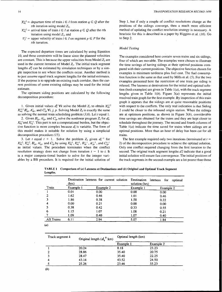
The examples considered here contain seven trains and six sidings, four of which are movable. The examples were chosen to illustrate the time savings of having sidings at their optimal positions com­pared with their current positions. The objective function chosen for examples is minimum tardiness plus fuel cost. The fuel consump­tion function is the same as that used by Mills et al. (5). For the two examples presented here the restriction of one train per siding is relaxed. The lateness at destinations for the initial and optimal solu­tion (both examples) are given in Table 1 (a), with the track segment lengths given in Table l(b). Figure 3(a) represents the initial resolved train graph for the first example. By inspection of this train graph it appears that the sidings are at quite reasonable positions with respect to the conflicts. The only real indication is that Siding 2 could be closer to the inbound origin station. When the sidings are at optimum positions, as shown in Figure 3(b), considerable time savings are obtained for the trains and they are kept closer to schedule throughout the journey. The second and fourth columns of Table l(a) indicate the time saved for trains ·when sidings are at optimal positions. More than an hour of delay has been cut for all trains.

The first example required only two iterations (terminated at t =

2) of the decomposition procedure to achieve the optimal solution. Only one conflict required changing from the first iteration to the second. The original track segment lengths dZ indicate that a good initial solution will ensure fast convergence. The initial positions of the track segments in the second example are a lot poorer than those

TABLE 1 Comparison of(a) Lateness at Destinations and (b) Original and Optimal Track Segment Lengths.

Destination lateness for current (hrs)

Train ExamEle 1 ExamEle 2 1 0.01 0.00 2 1.62 0.46 3 1.86 0.38 4 0.00 0.21 5 0.38 0.42 6 l.15 1.07 7 1.09 0.40 All Trains 6.11 2.94

(a)

Track segment k Original length (dk 0 km)

1 2 3 4 5

(b)

20.24 28.86 28.47 43.14 25.26'

solution Destination lateness for optimal solution (hrs) ExamEle 1 0.00 1.01 1.58 0.00 0.33 1.08 1.07 5.07

Optimal length (km)

Example 1 8.18 35.40 35.40 43.52 23.46

ExamEle 2 0.00 0.46 0.22 0.00 0.55 0.21 0.40 1.84

· ExamEle 2 23.23 20.75 22.25 24.50 55.23

Higgins et al. 15

Distance Distance

16 18 4 6 8 10 12 14 16 18 a Time (hrs) b Time (hrs)

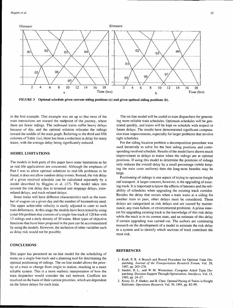
FIGURE 3 Optimal schedule given current siding positions (a) and given optimal siding positions (b).

in the first example. This example was set up so that most of the train interactions are toward the midpoint of the journey, where there are fewer sidings. The outbound trains suffer heavy delays because of this, and the optimal solution relocates the sidings toward the middle of the train graph. Referring to the third and fifth columns of Table l(a), there has been a reduction in delay for many trains, with the average delay being significantly reduced.

MODEL LIMIT A TIO NS

The models in both parts of this paper have some limitations as far as real-life applications are concerned. Although the emphasis of Part I was to allow optimal solutions to real-life problems to be found, it does not allow random delay events. Instead, the risk delay of a given resolved schedule can be calculated separately by a model described by Higgins et al. (17). The model takes into account the risk delay due_ to terminal and stoppage delays, train­related delays, and track-related delays.

Some trains will have different characteristics such as the num­ber of wagons on a given day and the number of locomotives used. The upper achievable velocity is easily adjusted to cater to such train differences. At this stage the models have been tested by using a real-life problem that consists of a single-line track of 120 km with 13 sidings and a daily density of 30 trains. Most types of objective functions that have been proposed in the past can be accommodated by using the models. However, the inclusion of other variables such as delay risk would not be possible.

CONCLUSIONS

This paper has presented an on-line model for the scheduling of trains on a single-line track and a planning tool for determining the optimal positioning of sidings. The on-line model allows the prior­ity of a train to change from origin to station, resulting in a more reliable system. This is a more realistic interpretation of how the train dispatcher would consider the rail network. Conflicts are resolved on the basis of their current priorities, which are dependent on the future delays for each train.

The on-line model will be useful to train dispatchers for generat­ing more reliable train schedules. Optimum schedules will be gen­erated quickly, and trains will be kept on schedule with respect to future delays. The results have demonstrated significant computa­tion time improvements, especially for larger problems that involve tight schedules.

For the siding location problem a decomposition procedure was used iteratively to solve for the best siding positions and corre­sponding reso)ved schedule. Results of the model have shown much improvement in delays to trains when the sidings are at optimal positions. If using this model to determine the positions of sidings only reduces the overall delay by a small percentage (while keep­ing the train costs uniform) then the long-term benefits may be large.

Positioning of sidings is one aspect of trying to optimize freight rail transport. A larger concern, however, is the upgrading of exist­ing track. It is important to know the effects oflateness and the reli­ability of schedules when upgrading the existing track corridor. Besides the delay that occurs when a train waits at a siding for another train to pass, other delays must be considered. These delays are categorized as risk delays and are caused by mainte­nance, any train failure, or environmental problems. A prime inter­est for upgrading existing track is the knowledge of this risk delay while the track is in its current state, and an estimate of this delay if certain upgrading was carried out. The authors are continuing research on the development of a model to estimate the risk delay to a system and to identify which sections of track contribute the most risk.

REFERENCES

1. Kraft, E. R. A Branch and Bound Procedure for Optimal Train Dis­patching. Journal of the Transportation Research Forum, Vol. 28, 1987' pp. 263-276.

2. Sauder, R. L., and W. M. Westerman. Computer Aided Train Dis­patching: Decision Support Through Optimisation. Interfaces, Vol. 13, 1983, pp. 24-27.

3. Kraay, D., P. Harker, and B. Chen. Optimal Pacing of Trains in Freight Railroads. Operations Research, Vol. 39, 1991, pp. 82-99.

16

4. Jovanovic, D., and P. Harker. Tactical Scheduling of Rail Operations: The SCAN I System. Transportation Science, Vol. 25, 1991, pp. 46-64.

5. Mills, R. G., S. E. Perkins, and P. J. Pudney. Dynamic Rescheduling of Long Haul Trains for Improved Timekeeping and Energy. Asia-Pacific Journal Operational Research, Vol. 8, 1991, pp." 146-165.

6. Higgins, A., E. Kozan, and L. Ferreira. An Improved Exact Solution Procedure for the Online Scheduling of Trains. Physical Infrastructure Research Report 36-94. Queensland University of Technology, Bris­bane, Australia, 1995.

7. Brooks, A., D. Kendrick, and A. Meeraus. GAMS: A User's Guide. Sci­entific Press, 1988.

8. Petersen, E. R., and A. J. Taylor. Design of a Single-Track Rail Line for High Speed Trains. Transportation Research A, Vol. 21, .1987, pp. 47-57.

9. Kraft, E. R. Analytical Models for Rail Line Capacity Analysis. Trans­portation Research Forum Proceedings, Vol. 23, 1983, pp. 461-471.

10. Mills, G., S. Perkins, and D. Sier. Capacity Planning for a Railway Cor­ridor. Proc., 12th National Conference of the Australian Society of Operations Research, 1983, pp. 470-487.

11. Petersen, E. R., A. J. Taylor, and C. D. Martland. An Introduction to Computer Assisted Train Dispatching. Journal of Advanced Trans­portation, Vol. 20, 1986, pp. 63-72.

TRANSPORTATION RESEARCH RECORD 1489

12. Geofferon, A. M. Generalised Benders Decomposition. Journal of Optimisation Theory and Applications, Vol. 10, 1972, pp. 237-263.

13. Koskosidis, Y. A., W. B. Powell, and M. M. Solomon. An Optimisation-Based Heuristic for Vehicle Routing and Scheduling with Soft Time Window Constraints. Transportation Science, Vol. 26, 1992, pp. 69-85.

14. Sklar, M. G., R. D. Armstrong, and S. Samn. Heuristics for Scheduling Aircraft and Crew During Airlift Operations. Transportation Science, Vol. 24, 1990, pp. 63-76.

15. Hohenbalken, B. V. Simplicial Decomposition in Non-Linear Pro­gramming Algorithms. Mathematical Programming, Vol. 13, 1974, pp. 49-68.

16. Higgins, A., E. Kozan, and L. Ferreira. Development of a Model to Optimise the Position of Crossing and Overtaking Loops on a Single Line Railway. Physical Infrastructure Research Report 16-94. Queens­land University of Technology, Brisbane, Australia, 1994.

17. Higgins, A., L. Ferreira, and E. Kozan. Modelling Delay Risks Associ­ated with Train Schedules. Transportation Planning and Technology, in press.

Publication of this paper sponsored by Committee on Electrification and Train Control Systems for Guided Ground Transportation Systems.

TRANSPORTATION RESEARCH RECORD 1489 17

Evaluation of Railway Subgrade Problems

D. Lr AND E. T. SELIG

The major causes contributing to railway subgrade problems are explained. Repeated dynamic loading, fine-grained soils, and excessive moisture content are indicated to be the major causes. The characteris­tics of different subgrade problems are discussed. Progressive shear failure, excessive plastic deformation, and subgrade attrition with mud pumping are the major problems for most railway subgrades under repeated traffic loading. The practical approaches for evaluation of sub­grade are discussed. To identify potential problem subgrade sites, the recommended approaches include the use of the available soil, geo­logic, and hydrologic information; visual inspection; study of track maintenance history; and analysis of track geometry car measurements. To assess subgrade conditions for a site known to have track foundation problems, the recommended approaches include the field subsurface inspection, laboratory tests, cone penetration test, and track stiffness test. For each of these approaches its application to the railway sub grade is analyzed and discussed.

Subgrade plays an important role in maintaining satisfactory per­formance of railway track under repeated traffic loads. Its role becomes even more critical when freight cars with heavier axle loads are introduced. In the past, the role of subgrade as the track foundation was not recognized adequately. Little effort was given to understanding the characteristics of subgrade soils under repeated traffic loading and environmental action. This situation has survived for a long time largely because a subgrade defect was often temporarily compensated for by repeatedly adding more ballast under ties or by frequent track maintenance. Thus, a lack of under­standing of the causes of or correcting the causes of subgrade prob­lems is then compensated for by higher track maintenance costs.

The objectives of this paper are to explain the causes and char­acteristics of subgrade problems and to discuss practical approaches for identifying and assessing them. The emphasis is on the existing soil subgrade or low-fill subgrade under repeated traffic loading.

CAUSESOFSUBGRADEPROBLEMS

Under unfavorable conditions various types of subgrad_e problems, as will be described later, can commence, develop, and lead to fail­ure or repeated railway track maintenance. The major causes that may contribute to the development of subgrade problems can be categorized into three groups: load factor, soil factor, and environ­mental factor (soil moisture and soil temperature). Often, however, a subgrade problem is a result of these factors acting together.

Load Factor

The load factor is the external factor that may cause a subgrade pr~blem. There are two types of loads: material self-weights and repeated dynamic loading. The first type of load can be a major fac-

Department of Civil and Environmental Engineering, University of Massa­chusetts, Amherst, Mass. 01003. (Current Address, D. Li: Transportation Technology Center, P.O. Box 11130, Pueblo, Colo. 81001.)

tor that may cause consolidation settlement or massive shear failure for a high embankment not properly designed or constructed. For a subgrade, however, the load factor of greatest concern is from repeated traffic loading.

Two features characterize the repeated traffic loading. One is the magnitude of the individual dynamic wheel load. The other is its number of repetitions. The subgrade behaves quite differently under a single static loading than under repeated traffic loading, even though the magnitudes of individual axle loads may be the same. For example, the subgrade, particularly subgrades of fine-grained soils such as silt and clay, will exhibit lower strengths under repeated loadings than under a single loading. Many track subgrade problems are associated with repeated loads. Therefore, it is neces­sary to take into account both the maximum magnitude of each indi­vidual load and the number of repetitions when considering the influence of load factor on subgrade performance.

Another important feature regarding the load factor that should be determined is the combined influence of all levels of repeated dynamic wheel loads. For a track sub grade the influence of repeated dynamic wheel loads smaller than the maximum can also be signif­icant. A simple example is that the subgrade settlement accumu­lated under smaller magnitudes of wheel loads with large numbers of repeated applications may be significantly larger than that gen­erated under a single application of a larger dynamic wheel loading. For detailed discussions and considerations of dynamic wheel load and repeated load applications, readers are referred to the work by Li (1), Li and Selig (2), and Raymond and Cai (3).

Soil Factor

A problem subgrade will not generally consist of coarse-grained soils (gravel and sand) but most likely will be fine-grained soils (silt and clay) because of the lower strength and permeability of the lat­ter materials. In general, the finer the soil or the greater the plastic­ity characteristics of the soil, the poorer the anticipated performance of this material as a railway track subgrade.

The influence of soil type on the subgrade performance is closely related to its moisture content and its susceptibility to the effects of moisture change. Most soils would have no problem acting as the subgrade if they could maintain a low enough moisture content. A major reason why subgrade problems are most commonly associ­ated with fine-grained soils is that the fine-grained soils are most susceptible to decreasing in strength and stiffness with increasing water content and do not drain well. On the other hand, the perfor­mance properties of most coarse-grained soils are less significantly influenced by the presence of water, and such soils can drain well so that they usually have low moisture contents.

Soil Moisture

Almost every subgrade problem can be attributed to the high mois­ture content in the fine-grained soil subgrade. The presence of water

18

in the subgrade can reduce the strength and stiffness of subgrade soils dramatically. If a subgrade maintains low enough moisture content throughout the year and if it is assumed that the ballast and subballast layers are properly graded and sufficiently thick, the subgrade should not be the cause of the need for excessive main­tenance.

A subgrade may become wet or saturated by the infiltration of water from the surface or from groundwater. According to experi­ence gained from work on highways ( 4) the major factor influenc­ing the moisture content of the subgrade is the groundwater if the water table is within approximately 6.1 m (20 ft) of the surface. However, for a subgrade in which the water table is greater than 6.1 m deep, the moisture content in the upper part of the subgrade is determined primarily by seasonal variation caused by rainfall, dry­ing conditions, and soil suction.

The duration of water contact with a subgrade soil may make a large difference in the resulting strength of the soil. A clay sub grade exposed to the air with occasional rain showers and dry periods may stay strong, whereas a subgrade covered by ballast and subballast (which cuts off evaporation) may get weak. The ballast and subbal­last allow water to penetrate, but they do not allow it to evaporate. As a result a subgrade that is not free-draining invariably can be saturated.

Soil Temperature

Soil temperature is of concern when it causes cycles of freezing and thawing. Under certain combinations of temperature, soil suction, soil permeability, and availability of water, ice lenses will form when the soil freezes, causing ground heave. When the soil thaws again excess water from the ice lens will cause weakening of the soil.

CHARACTERISTICS OF SUBGRADE PROBLEMS

Subgrade problems can be divided into three groups in terms of their major causes. The first group includes those problems primar­ily caused by repeated traffic loading. The second group includes those problems primarily caused by the weight of the track struc­ture, subgrade, and train. The third group includes those problems primarily caused by the environmental factors such as freezing soil temperature and changing soil moisture content. In general, the traf­fic load-induced subgrade problems occur at shaUower depths in the subgrade. The environmental subgrade problems also occur at shal­lower depths or occur at the surfaces of subgrade slopes. The weight-induced subgrade problems caused by the track structure, subgrade, and train, on the other hand, involve massive movement of the subgrade soils and are generally more deep-seated in nature.

Table I summarizes the subgrade problems, their causes, and their features that were categorized. The first four types are primar­ily caused by repeated traffic loading. The second two types are those mainly caused by the weight of the train, track, and subgrade. The last four types are those related to environmental factors. The following provides a detailed discussion of the first three types of subgrade problems, that is, those major problems for an existing low-fill subgrade under repeated traffic loading.

Progressive Shear Failure

Progressive shear failure is the plastic flow of the soil caused by overstressing at the subgrade surface by the repeated loading. The

TRANSPORTATION RESEARCH RECORD 1489

subgrade soil gradually squeezes outward and upward following the path of least resistance. This type of failure is illustrated in Figure 1 (5) and has been observed in both revenue service tracks and the FAST test track in the United States. This is primarily a problem with fine-grained soils, particularly those with a high clay content. Such soils soften as their moisture content increases and reduce in strength because of remolding and the development of increased pore water pressure from repeated loading.

As shown in Figure 1 heave of material at the track side is matched by a corresponding depression beneath the track. This depression is reflected at the surface as a depression in the track sub­structure, which is corrected by the addition of ballast beneath the ties. The addition of more ballast results in an increase in ballast depth and a corresponding reduction in soil stress at the subgrade level, which tends to improve sub grade stability. However, the depression traps water, which tends to cancel the potential improve­ment. Therefore, only adding more ballast without correcting the distorted subgrade surface configuration to provide drainage will not correct the stability problem caused by the progressive shear failure.

Excessive Plastic Deformation

·Although progressive shear failure is accompanied by progressive shear deformation in the subgrade, excessive plastic deformation is classified here as a separate type of subgrade problem. It includes not only the vertical component of progressive shear deformation but also the vertical deformation caused by progressive compaction and consolidation of subgrade soils under repeated traffic loads.

The development of cumulative plastic deformation in the sub­grade is a function of the repeated loading. The plastic deformation produced by a single axle load is essentially negligible under nor­mal conditions. However, the plastic deformation in the subgrade may accumulate to such a significant level with repeated load appli­cations that it can severely affect the performance of the track. Moreover, the development of plastic deformation is usually nonuniform along and across the track. Hence, excessive plastic deformation can lead to unacceptable track geometry change.

The development of excessive plastic deformation is more rapid for a newly constructed subgrade and for a cohesive soil subgrade with access to water. In the latter case, with the same mechanism as that for the progressive shear failure, when a depression at the sub­grade surface occurs, it collects water, causing an increased soften­ing of the subgrade near the depression. With repeated loading the clay squeezes out and the underlying clay in tum softens; thus, the depression deepens and the ridges of soft subgrade material collect around the pocket, which forms a larger water-filled pocket.

To offset the loss of track elevation caused by the excessive plas­tic deformation in the subgrade, more ballast material generally must be added to the track, which results in an increased depth of ballast material. When ballast continues to replace the subgrade soil and as it is repeatedly added under the ties, a severe manifestation of accumulated subgrade plastic deformation, termed baUast pocket, can form. Figures 2(a) and 2(b) illustrate examples of a bal­last pocket across and along the track. As discussed earlier, although adding more ballast increases the ballast depth, this cannot com­pletely solve the problem of excessive plastic deformation devel­opment since the ballast pocket traps water, which in tum leads to softening of the subgrade soils. Furthermore, the ballast may become contaminated with the subgrade soil particles, thereby degrading the characteristics of the ballast or the granular material.

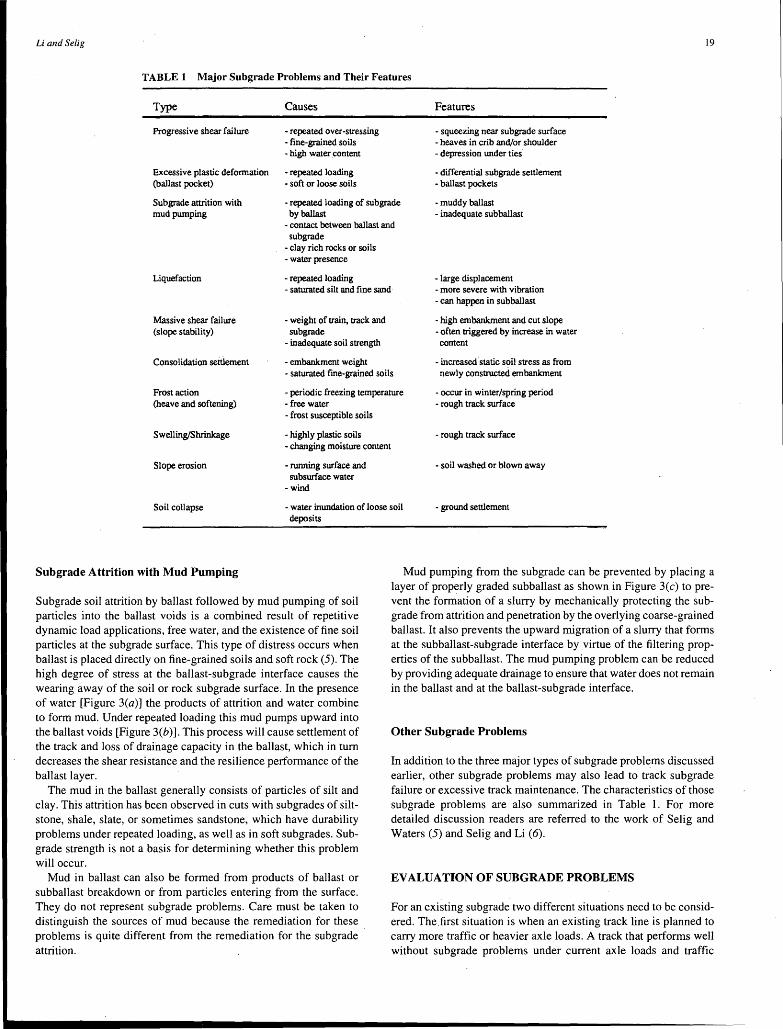
Li and Selig 19

TABLE 1 Major Subgrade Problems and Their Features

Type

Progressive shear failure

Excessive plastic deformation (ballast pocket)

Causes

- repeated over-stressing - fine-grained soils - high water content

- repeated loading - soft or loose soils

Features

- squeezing near subgrade surface - heaves in crib and/or shoulder - depression under ties

- differential subgrade settlement - ballast pockets

Subgrade attrition with mud pumping

- repeated loading of subgrade by ballast

- muddy ballast - inadequate subballast

- contact between ballast and subgrade

- clay rich rocks or soils - water presence

Liquefaction - repeated loading - large displacement - saturated silt and fine sand - more severe with vibration

Massive shear failure (slope stability)

Consolidation settlement

- weight of train, track and subgrade

- inadequate soil strength

- embankment weight

- can happen in subballast

- high embankment and cut slope - often triggered by increase in water content

- saturated fine-grained soils - increased static soil stress as from newly constructed embankment

Frost action - periodic freezing temperature - occur in winter/spring period (heave and softening)

Swelling/Shrinkage

Slope erosion

-free water - frost susceptible soils

- highly plastic soils - changing moisture content

- running surface and subsurface water

-wind

- rough track surface

- rough track surface

- soil washed or blown away

Soil collapse - water inundation of loose soil deposits

- ground settlement

Subgrade Attrition with Mud Pumping

Subgrade soil attrition by ballast followed by mud pumping of soil particles into the ballast voids is a combined result of repetitive dynamic load applications, free water, and the existence of fine soil particles at the subgrade surface. This type of distress occurs when ballast is placed directly on fine-grained soils and soft rock (5). The high degree of stress at the ballast-subgrade interface causes the wearing away of the soil or rock subgrade surface. In the presence of water [Figure 3(a)] the products of attrition and water combine to form mud. Under repeated loading this mud pumps upward into the ballast voids [Figure 3(b)]. This process will cause settlement of the track and loss of drainage capacity in the ballast, which in tum decreases the shear resistance and the resilience performance of the ballast layer.

The mud in the ballast generally consists of particles of silt and clay. This attrition has been observed in cuts with subgrades of silt­stone, shale, slate, or sometimes sandstone, which have durability problems under repeated loading, as well as in soft subgrades. Sub­grade strength is not a basis for determining whether this problem will occur.

Mud in ballast can also be formed from products of ballast or subballast breakdown or from particles entering from the surface. They do not represent subgrade problems. Care must be taken to distinguish the sources of mud because the remediation for these _ problems is quite different from the remediation for the subgrade attrition.

Mud pumping from the subgrade can be prevented by placing a layer of properly graded subballast as shown in Figure 3(c) to pre­vent the formation of a slurry by mechanically protecting the sub­grade from attrition and penetration by the overlying coarse-grained ballast. It also prevents the upward migration of a slurry that forms at the subballast-subgrade interface by virtue of the filtering prop­erties of the subballast. The mud pumping problem can be reduced by providing adequate drainage to ensure that water does not remain in the ballast and at the ballast-subgrade interface.

Other Subgrade Problems

In addition to the three major types of subgrade problems discussed earlier, other subgrade problems may also lead to track subgrade failure or excessive track maintenance. The characteristics of those subgrade problems are also summarized in Table 1. For more detailed discussion readers are referred to the work of Selig and Waters (5) and Selig and Li (6).

EVALUATION OF SUBGRADE PROBLEMS

For an existing subgrade two different situations need to be consid­ered. The.first situation is when an existing track line is planned to carry more traffic or heavier axle loads. A track that performs well without subgrade problems under current axle loads and traffic

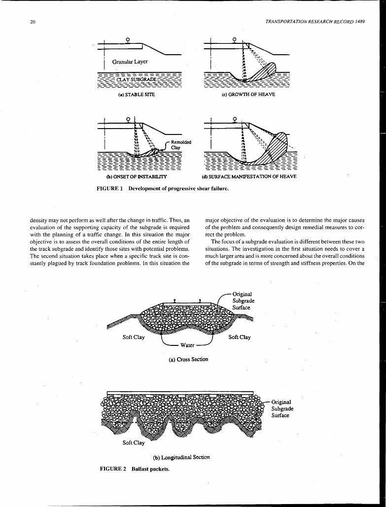
20

Granular Layer

(a) STABLE SITE

Re molded Qay

----· [~~~~~~~~~~~~~~-

(b) ONSET OF INST ABILITY

TRANSPORTATION RESEARCH RECORD 1489

---------------=----------~~~~ - - - - -~~~~~~=-=-==-=-==-~~~~~~

(c) GROWTII OF HEAVE

----. ..%"""""~_...ii!!!"'":~-=--=--=-~ ~~~£~~-::-=:-=:-=:-::~-=-~~~

(d) SURFACE MANIFESTATION OF HEAVE

FIGURE 1 Development of progressive shear failure.

density may not perform as well after the change in traffic. Thus, an evaluation of the supporting capacity of the subgrade is required with the planning of a traffic change. In this situation the major objective is to assess the overall conditions of the entire length of the track subgrade and identify those sites with potential problems. The second situation takes place when a specific track site is con­stantly plagued by track foundation problems. In this situation the

Soft Clay

major objective of the evaluation is to determine the major causes of the problem and consequently design remedial measures to cor­rect the problem.

The focus of a subgrade evaluation is different between these two situations. The investigation in the first situation needs to cover a much larger area and is more concerned about the overall conditions of the subgrade in terms of strength and stiffness properties. On the

Soft Clay

(a) Cross Section

Soft Clay

(b) Longitudinal Section

FIG URE 2 Ballast pockets.

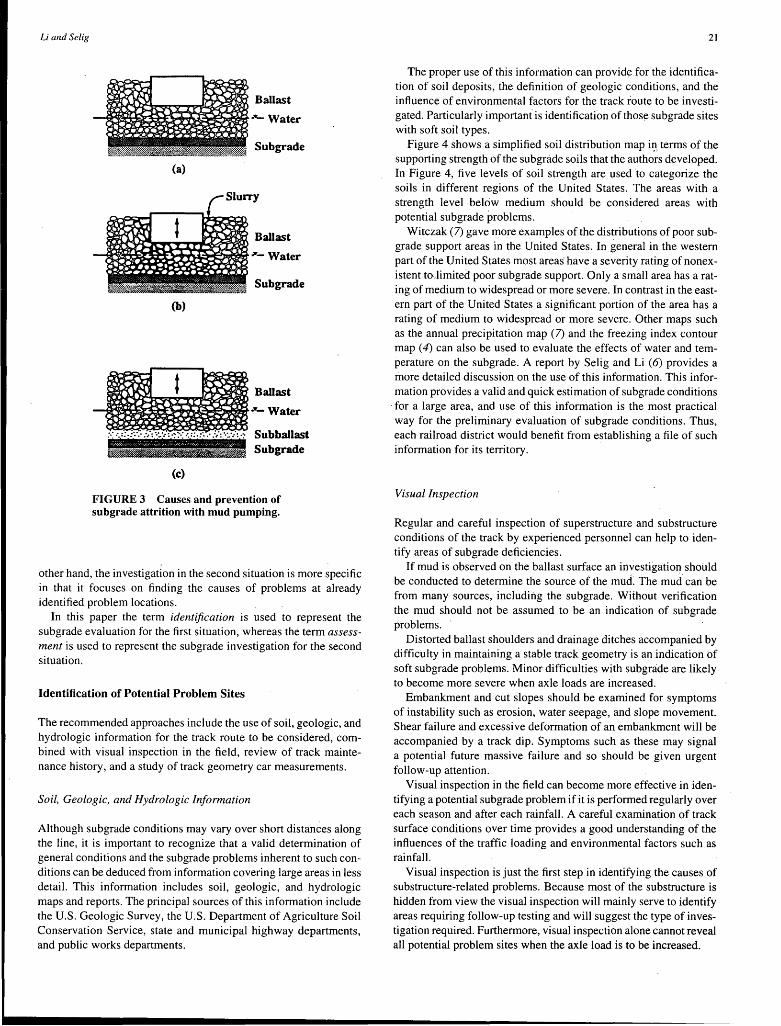
Li and Selig

(a)

(b)

(c)

FIGURE 3 Causes and prevention of subgrade attrition with mud pumping.

other hand, the investigation in the second situation is more specific in that it focuses on finding the causes of problems at already identified problem locations.

In this paper the term identification is used to represent the subgrade evaluation for the first situation, whereas the term assess­ment is used to represent the subgrade investigation for the second situation.

Identification of Potential Problem Sites

The recommended approaches include the use of soil, geologic, and hydrologic information for the track route to be considered, com­bined with visual inspection in the field, review of track mainte­nance history, and a study of track geometry car measurements.

Soil, Geologic, and Hydrologic Information

Although subgrade conditions may vary over short distances along the line, it is important to recognize that a valid determination of general conditions and the subgrade problems inherent to such con­ditions can be deduced from information covering large areas in less detail. This information includes soil, geologic, and hydrologic maps and reports. The principal sources of this information include the U.S. Geologic Survey, the U.S. Department of Agriculture Soil Conservation Service, state and municipal highway departments, and public works departments.

21

The proper use of this information can provide for the identifica­tion of soil deposits, the definition of geologic conditions, and the influence of environmental factors for the track route to be investi­gated. Particularly important. is identificatfon of thos~ subgrade sites with soft soil types.

Figure 4 shows a simplified soil distribution map i~, terms of the supporting strength of the sub grade soils that the authors developed. In Figure 4, five levels of soil strength are used to categorize the soils in different regions of the United States. The areas with a strength level below medium should be considered areas with potential subgrade problems.

Witczak (7) gave more examples of the distributions of poor sub­grade support areas in the United States. In general in the western part of the United States most areas· have a severity rating of nonex­istent to.limited poor subgrade support. Only a small area has a rat­ing of medium to widespread or more severe. In contrast in the east­ern part of the United States a significant portion of the area has a rating of medium to widespread or more severe. Other maps such as the annual precipitation map (7) and the freezing index contour map ( 4) can also be used to evaluate the effects of water and tem­perature on the subgrade. A report by Selig and Li (6) provides a more detailed discussion on the use of this information. This infor­mation provides a valid and quick estimation of subgrade conditions

· for a large area, and use of this information is the most practical way for the preliminary evaluation of subgrade conditions. Thus, each railroad district would benefit from establishing a file of such information for its territory.

Visual Inspection

Regular and careful inspection of superstructure and substructure conditions of the track by experienced personnel can help to iden­tify areas of subgrade deficiencies.

If mud is observed on the ballast surface an investigation should be conducted to determine the source of the mud~ The mud can be from many sources, including the subgrade. Without verification the mud should not be assumed to be an indication of subgrade problems.

Distorted ballast shoulders and drainage ditches accompanied by difficulty in maintaining a stable track geometry is an indication of soft subgrade problems. Minor difficulties with subgrade are likely to become more severe when axle loads are increased.

Embankment and cut slopes should be examined for symptoms of instability such as erosion, water seepage, and slope movement. Shear failure and excessive deformation of an embankment will be accompanied by a track dip. Symptoms such as these may signal a potential future massive failure and so should be given urgent follow-up attention.

Visual inspection in the field can become more effective in iden­tifying a potential subgrade problem if it is performed regularly over each season and after each rainfall. A careful examination of track surface conditions over time provides a good understanding of the influences of the traffic loading and environmental factors such as rainfall.

Visual inspection is just the first step in identifying the causes of substructure-related problems. Because most of the substructure is hidden from view the visual inspection will mainly serve to identify areas requiring follow-up testing and will suggest the type of inves­tigation required. Furthermore, visual inspection alone cannot reveal all potential problem sites when the axle load is to be increased.

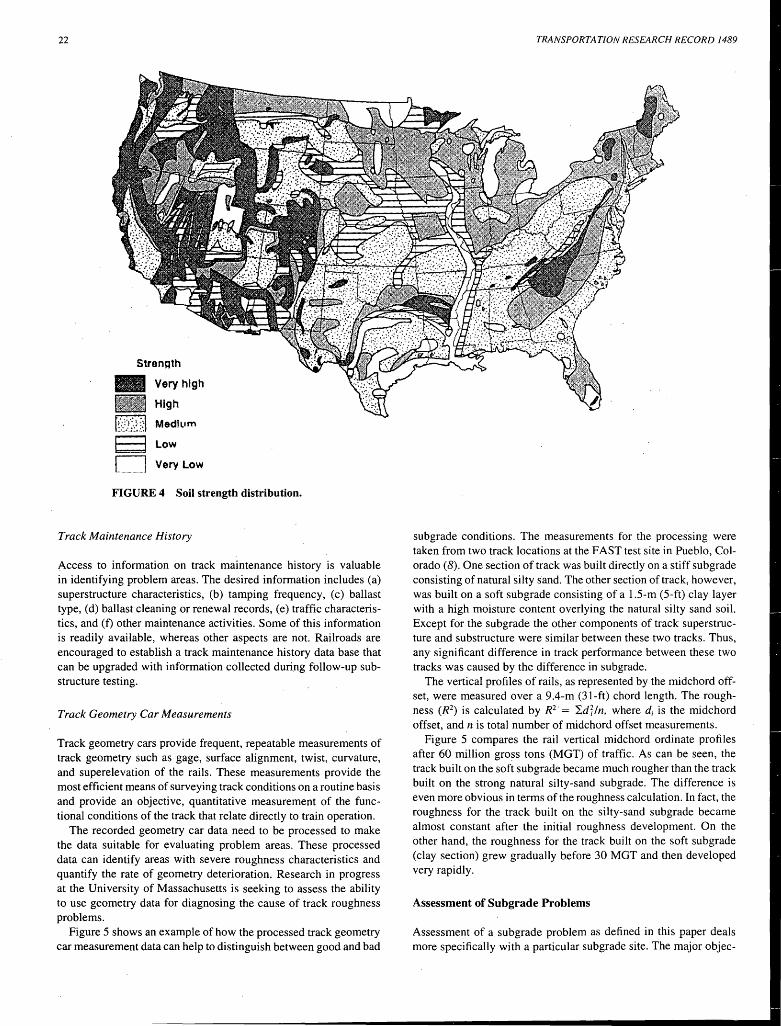
22

Strength

- Veryhlgh

High

kD\~Jd MediL•m

a low

L .......... u.J Very LOW

FIGURE 4 Soil strength distribution.

Track Maintenance History

Access to information on track maintenance history is valuable in identifying problem areas. The desired information includes (a) superstructure characteristics, (b) tamping frequency, ( c) ballast type, (d) ballast cleaning or renewal records, (e) traffic characteris­tics, and (f) other maintenance activities. Some of this information is readily available, whereas other aspects are not. Railroads are encouraged to establish a track maintenance history data base that can be upgraded with information collected during follow-up sub­structure testing.

Track Geometry Car Measurements

Track geometry cars provide frequent, repeatable measurements of track geometry such as gage, surface alignment, twist, curvature, and superelevation of the rails. These measurements provide the most efficient means of surveying track conditions on a routine basis and provide an objective, quantitative measurement of the func­tional conditions of the track that relate directly to train operation.

The recorded geometry car data need to be processed to make the data suitable for evaluating problem areas. These processed data can identify areas with severe roughness characteristics and quantify the rate of geometry deterioration. Research in progress at the University of Massachusetts is seeking to assess the ability to use geometry data for diagnosing the cause of track roughness problems.

Figure 5 shows an example of how the processed track geometry car measurement data can help to distinguish between good and bad

TRANSPORTATION RESEARCH RECORD 1489

subgrade conditions. The measurements for the processing were taken from two track locations at the FAST test site in Pueblo, Col­orado ( 8). One section of track was built directly on a stiff sub grade consisting of natural silty s·and. The other section of track, however, was built on a soft subgrade consisting of a 1.5-m (5-ft) clay layer with a high moisture content overlying the natural silty sand soil. Except for the subgrade the other components of track superstruc­ture and substructure were similar between these two tracks. Thus, any significant difference in track performance between these two tracks was caused by the difference in subgrade.

The vertical profiles of rails, as represented by the midchord off­set, were measured over a 9 .4-m (31-ft) chord length. The rough­ness (R2

) is calculated by R2 · = ""i..d71n, where d; is the midchord offset, and n is total number of midchord offset measurements.

Figure 5 compares the rail vertical midchord ordinate profiles after 60 million gross tons (MGT) of traffic. As can be seen, the track built on the soft subgrade became much rougher than the track built on the strong natural silty-sand subgrade. The difference is even more obvious in terms of the roughness calculation. In fact, the roughness for the track built on the silty-sand subgrade became almost constant after the initial roughness development. On the other hand, the roughness for the track built on the soft subgrade (clay section) grew gradually before 30 MGT and then developed very rapidly.

Assessment of Subgrade Problems

Assessment of a subgrade problem as defined in this paper deals more specifically with a particular subgrade site. The major objec-

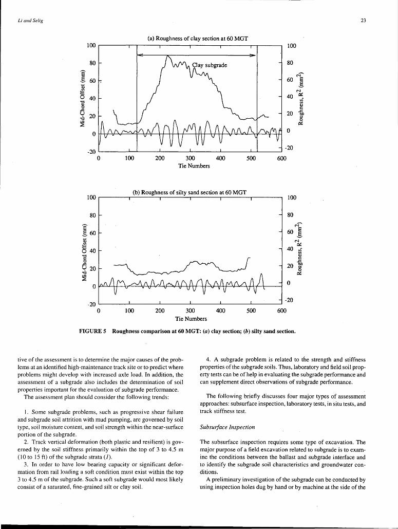
Li and Selig 23

(a) Roughness of clay section at 60 MGT 100 100

80 80

I N-

60 - 60 l ~ ell N :::::

40 ~ 0 40 rn 'E ell

0 0 c: .c fo u 20 20 .0 5 ~ ~

0 0

-20 -20

0 100 200 300 400 500 600 Tie Numbers

(b) Roughness of silty sand section at 60 MGT 100 .--~~~-r-~~~---..--~~~...-~~~---...~~~~...-~~~--. 100

.... 0

80

.t: 0 40 'E 0

a 20 .0 ~

80

60

40

20

0

-20 -20 .___~~~--~~~~'--~~~_._~~~__..~~~~_._~~~--'

0 100 200 300 400 500 600

N-e g

N ~ rn <ll Cl) c: .c bl)

5 ~

Tie Numbers

FIGURES Roughness comparison at 60 MGT: (a) clay section; (b) silty sand section.

tive of the assessment is to determine the major causes of the prob­lems at an identified high-maintenance track site or to predict where problems might develop with increased axle load. In addition, the assessment of a subgrade also includes the determination of soil properties important for the evaluation of subgrade performance.

The assessment plan should consider the following trends:

1. Some subgrade problems, such as progressive shear failure and subgrade soil attrition with mud pumping, are governed by soil type, soil moisture content, and soil strength within the near-surface portion of the subgrade.

2. Track vertical deformation (both plastic and resilient) is gov­erned by the soil stiffness primarily within the top of 3 to 4.5 m (10 to 15 ft) of the sub grade strata (1).

3. In order to have low bearing capacity or significant defor­mation from rail loading a soft condition must exist within the top 3 to 4.5 m of the subgrade. Such a soft subgrade would most likely consist of a saturated, fine-grained silt or clay soil.

4. A subgrade problem is related to the strength and stiffness properties of the sub grade soils. Thus, laboratory and field soil prop­erty tests can be of help in evaluating the sub grade performance and can supplement direct observations of subgrade performance.

The following briefly discusses four major types of assessment approaches: subsurface inspection, laboratory tests, in situ tests, and track stiffness test.

Subsurface Inspection

The subsurface inspection requires some type of excavation. The major purpose of a field excavation related to subgrade is to exam­ine the conditions between the ballast and subgrade interface and to identify the subgrade soil characteristics and groundwater con-ditions. ·

A preliminary investigation of the subgrade can be conducted by using inspection holes dug by hand or by machine at the side of the

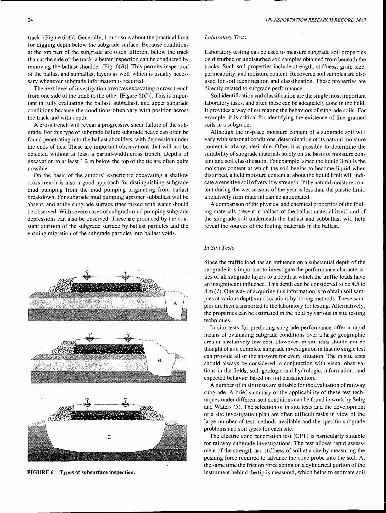
24

track [(Figure 6(A)]. Generally, 1 m or so is about the practical limit for digging depth below the subgrade surface. Because conditions at the top part of the subgrade are often different below the track than at the side of the track, a better inspection can be conducted by removing the ballast shoulder [Fig. 6(B)]. This permits inspection of the ballast and subballast layers as well, which is usually neces­sary whenever subgrade information is required.

The next level of investigation involves excavating a cross trench from one side of the track to the other [Figure 6(C)]. This is impor­tant in fully evaluating the ballast, subballast, and upper subgrade conditions because the conditions often vary with position across the track and with depth.

A cross trench will reveal a progressive shear failure of the sub­grade. For this type of subgrade failure subgrade heave can often be found penetrating into the ballast shoulders, with depression under the ends of ties. These are important observations that will not be detected without at least a partial'-width cross trench. Depths of excavation to at least 1.2 m below the top of the tie are often quite possible.

On the basis of the authors' experience excavating a shallow cross trench is also a good approach for distinguishing subgrade mud pumping from the mud pumping originating from ballast breakdown. For subgrade mud pumping a proper subballast will be absent, and at the subgrade surface fines mixed with water should be observed. With severe cases of sub grade mud pumping sub grade depressions can also be observed. These are produced by the con­stant attrition of the subgrade surface by ballast particles and the ensuing migration of the subgrade particles into ballast voids.

... --~·-·----~--~ .... !: .- ··, .':' p

FiGURE 6 Types of subsurface inspection.

TRANSPORTATION RESEARCH RECORD 1489

. Laboratory Tests

Laboratory testing can be used to measure subgrade soil properties on disturbed or undisturbed soil samples obtained from beneath the tracks. Such soil properties include strength, stiffness, grain size, permeability, and moisture content. Recovered soil samples are also used for soil identification and classification. These properties are directly related to subgrade performance.

Soil identification and classification are the single most important laboratory tasks, and often these can be adequately done in the field. It provides a way of estimating the behaviors of subgrade soils. For example, it is critical for identifying the existence of fine-grained soils in a subgrade.

Although the in-place moisture content of a subgrade soil will vary with seasonal conditions, determination of its natural moisture content is always desirable. Often it is possible to determine the suitability of subgrade materials solely on the basis of moisture con­tent and soil classification. For example, since the liquid limit is the moisture content at which the soil begins to become liquid when disturbed, a field moisture content at about the liquid limit will indi­cate a sensitive soil of very low strength. If the natural moisture con­tent during the wet seasons of the year is less than the plastic limit, a relatively firm material can be anticipated.

A comparison of the physical and chemical properties of the foul­ing materials present in ballast, of the ballast material itself, and of the subgrade soil underneath the ballast and subballast will help reveal the sources of the fouling materials in the ballast.

In Situ Tests

Since the traffic load has an influence on a substantial depth of the subgrade it is important to investigate the performance characteris­tics of all subgrade layers to a depth at which the traffic loads have an insignificant influence. This depth can be considered to be 4.5 to 8 m (1). One way of acquiring this information is to obtain soil sam­ples at various depths and locations by boring methods. These sam­ples are then transported to the laboratory for testing. Alternatively, the properties can be estimated in the field by various in situ testing techniques.

In situ tests for predicting subgrade performance offer a rapid means of evaluating subgrade conditions over a large geographic area at a relatively low cost. However, in situ tests should not be thought of as a complete subgrade investigation in that no single test can provide all of the answers for every situation. The in situ tests should always be considered in conjunction with visual observa­tions in the fields, soil, geologic and hydrologic, information; and expected behavior based on soil classification.

A number of in situ tests are suitable for the evaluation of railway subgrade. A brief summary of the applicability of these test tech­niques under different soil conditions can be found in work by Selig and Waters (5). The selection of in situ tests and the development of a site investigation plan are often difficult tasks in view of the large number of test methods available and the specific subgrade problems and soil types for each site.

The electric cone penetration test (CPT) is particularly suitable for railway subgrade investigations. The test allows rapid assess­ment of the strength and stiffness of soil at a site by measuring the pushing force required to advance the cone probe into the soil. At the same time the friction force acting on a cylindrical portion of the instrument behind the tip is measured, which helps to estimate soil

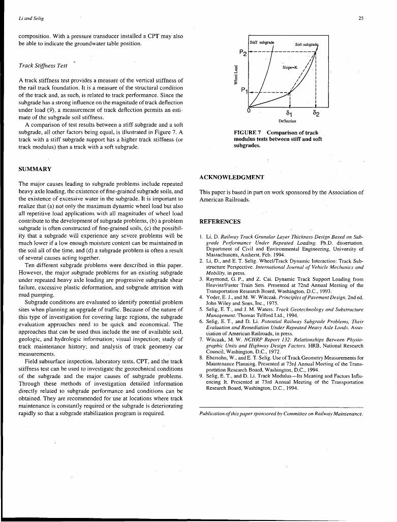
Li and Selig

composition. With a pressure transducer installed a CPT may also be able to indicate the groundwater table position.

Track Stiffness Test

A track stiffness test provides a measure of the vertical stiffness of the rail track foundation. It is a measure of the structural condition of the track and, as such, is related to track performance. Since the sub grade has a strong influence on the magnitude of track deflection under load (9), a measurement of track deflection permits an esti­mate of the subgrade soil stiffness.

A comparison of test results between a stiff subgrade and a soft subgrade, all other factors being equal, is illustrated in Figure 7. A track with a stiff sub grade support has a higher track stiffness (or track modulus) than a track with a soft subgrade.

SUMMARY

The major causes leading to subgrade problems include repeated heavy axle loading, the existence of fine-grained subgrade soils, and the existence of excessive water in the subgrade. It is important to realize that (a) not only the maximum dynamic wheel load but also all repetitive load applications with all magnitudes of wheel load contribute to the development of sub grade problems, (b) a problem subgrade is often constructed of fine-grained soils, (c) the possibil­ity that a subgrade will experience any severe problems will be much lower if a low enough moisture content can be maintained in the soil all of the time, and (d) a subgrade problem is often a result of several causes acting together.

Ten different subgrade problems .were described in this paper. However, the major subgrade problems for an existing subgrade under repeated heavy axle loading are progressive subgrade shear failure, excessive plastic deformation, and subgrade attrition with mud pumping.

Subgrade conditions are evaluated to identify potential problem sites when planning an upgrade of traffic. Because ofthe nature of tbis type of investigation for covering large regions, the subgrade evaluation approaches need to be quick and economical. The approaches that can be used thus include the use of available soil, geologic, and hydrologic information; visual inspection; study of track maintenance history; and analysis of track geometry car measurements.

Field subsurface inspection, laboratory tests, CPT, and the track stiffness test can be used to investigate the geotechnical conditions of the subgrade and the major causes of subgrade problems. Through these methods of investigation detailed information directly related to subgrade performance and conditions can be obtained. They are recommended for use at locations where track maintenance is constantly required or the subgrade is deteriorating rapidly so that a subgrade stabilization program is required.

Deflection

FIGURE 7 Comparison of track modulus tests between stiff and soft subgrades.

ACKNOWLEDGMENT

25

This paper is based in part on work sponsored by the Association of American Railroads.

REFERENCES

1. Li, D. Railway Track Granular Layer Thickness Design Based on Sub­grade Performance Under Repeated Loading. Ph.D. dissertation. Department of Civil and Environmental Engineering, University of Massachusetts, Amherst, Feb. 1994.

2. Li, D., and E. T. Selig. Wheelffrack Dynamic Interaction: Track Sub­structure Perspective. International Journal of Vehicle Mechanics and Mobility, in press.

3. Raymond, G. P., and Z. Cai. Dynamic Track Support Loading from Heavier/Faster Train Sets. Presented at 72nd Annual Meeting of the Transportation Research Board, Washington, D.C., 1993.

4. Yoder, E. J., and M. W. Witczak. Principles of Pavement Design, 2nd ed. John Wiley and Sons, Inc., 1975.

5. Selig, E. T:, and J.M. Waters. Track Geotechnology and Substructure Management.· Thomas Telford Ltd., 1994.

6 .. Selig, E. T., and D. Li. Potential. Railway Sub grade Problems, Their Evaluation and Remediation Under Repeated Heavy Axle Loads. Asso­ciation of American Railroads, in press.

7. Witczak, M. W. NCHRP Report 132: Relationships Between Physio­graphic Units and Highway Design Factors. HRB, National Research Council, Washington, D.C., 1972.

8. Ebersohn, W., and E.T. Selig. Use of Track Geometry Measurements for Maintenance Planning. Presented at 73rd Annual Meeting of the Trans­portation Research Board, Washington, D.C., 1994.

9. Selig, E. T., and D. Li. Track Modulus-Its Meaning and Factors Influ­encing It. Presented at 73rd Annual Meeting of the Transportation Research Board, Washington, D.C., 1994.

Publication of this paper sponsored by Committee on Railway Maintenance.

26 TRANSPORTATION RESEARCH RECORD 1489

Development of Nonconventional Tie and Track Structure Inspection Systems

ALLAN M. ZAREMBSKI AND WILLIAM T. McCARTHY

During the last decade research has focused on new and improved track inspection techniques to define the conditions of the track structure and its key components. Among the areas of focus for this research have been inspection of the strength or load-carrying ability of the track structure and inspection of the cross-ties and cross-tie/fastener systems. The results of two cooperative research and development programs in this area performed by Burlington Northern Railroad and Tiescan, Inc., a joint venture company consisting of ZETA-TECH Associates, Inc., Holland Company, and De Beer Applied Research Company, are pre­sented. The two research programs are as follows: the development and implementation of the Track Strength Analysis and Recording system, a hi-rail-based system for the measurement of track strength (gage strength under applied load) and track geometry, and the development and implementation of the Tiescan wood cross-tie inspection system, a continuous wood tie condition measurement system. In the case of both systems a research concept was taken and transformed into a prototype production inspection system. Both systems are currently undergoing final system shakedown and validation.

The concept of the measurement of the strength or load-carrying capacity of the track, and in particular the gage strength or gage restraint of the track, was originally introduced as part of the Asso­ciation of American Railroad's (AAR's) Track Strength Character­ization Program in the late 1970s (J). As part of that program a sys­tem for the continuous in-track measurement of track strength was first demonstrated by using a specially developed research vehicle dubbed the Decarotor (2,3). The Decarotor was developed· for use in evaluating the gage strength of the track and identifying weak points in the track. Tests with this system showed that under con­trolled loading conditions, that is, significant lateral and vertical loads applied to the railhead, the deflection of the track, and specif­ically, the gage widening under these loads, serves as a direct indi­cator of track gage strength. Furthermore, under properly defined levels of loading, this testing does not cause permanent damage to the track structure (2,3).

The success of the Decarotor tests led to the development of second- and third-generation test systems. The Volpe Transporta­tion Systems Center (VTSC) developed a gage-spreading split axle for measuring rail restraint (4). AAR followed with their Track Loading Vehicle (5,6.).

VTSC' s Gage Restraint Measurement System (GRMS) uses split axle technology coupled with an instrumented wheel set to apply and measure vertical and lateral loads on the railhead. This axle is mounted in a standard truck assembly on an open-top hopper car that operates in a train consisting of a locomotive, the hopper car, and an instrumentation/support car. An exception report is gener-

A. M. Zarembski, ZETA-TECH Associates, Inc., 900 Kings Highway North, Suite 208, Cherry Hill, N. J. 08034. W. T. McCarthy, Burlington Northern Railroad, 1900 Continental Plaza, 777 Main Street, Fort Worth, Tex. 76102.

ated onboard the car, and a tie renewal recommendation is made after the test. To date GRMS has more than 8,047 km (5,000 mi) of production testing, during which the system performed consistently and accurately (4).

AAR' s Track Loading Vehicle (TL V) was developed as a research platform to study the effects that dynamic track loads have on track and track components (5,6). Forces are measured by using an instrumented wheel set mounted in a load bogie under a rebuilt locomotive frame. The TL V is placed in consist with a locomotive and an instrumentation/support car.

These research and development activities by AAR and VTSC have shown that gage loading systems can be used to accurately measure the ability of track to resist gage widening forces. Gage strength measurements have been used to locate potential derail­ment conditions, assess fastener strength, and prioritize tie renewals. Recognizing these benefits, Burlington Northern Railroad (BN) commissioned the development of the Track Strength Analy­sis and Recording system (TSAR) from Tiescan, Inc., a consortium comprising of ZETA-TECH Associates, Inc., Holland, Inc., and De Beer Applied Research Company. This system was designed as a production track strength and track geometry measurement system mounted on a hi-rail vehicle to facilitate movement across the BN system.

DESCRIPTION OF TSAR

TSAR is composed of a test platform, a track loading axle, track geometry instrumentation, and an integrated software analysis and reporting system. The test platform is a three-axle, 18-kg (20-ton) truck equipped for highway and hi-rail travel (Figure 1). While on rail the vehicle has a gross weight of 22,679 kg (50,000 lbs) on two axles. The rear axle (split axle) provides propulsion and braking, applies up to 5,443 kg ( 12,000 lbs) of lateral load per rail and 6,803 kg (15,000 lbs) of vertical load per rail, and measures loaded gage (Figure 2). The vehicle measures both track geometry and gage strength while moving forward at speeds of up to 40 kph (25 mph) on track with curvatures of up to 12 degrees. Results are output on a chart recorder (Figure 3), which displays both track geometry and track strength (gage restraint or reserve) on exception reports, and data are also continuously stored onboard the vehicle.

Although most geometry and gage restraint testing to date has focused on heavy test vehicles with axle loadings comparable to those of heavy-axle-load freight equipment, hi-rail types of vehicles offer a degree of flexibility and ease of use that make them attrac­tive. By combining both sets of capabilities, track strength mea­surement and track geometry measurement, on a single vehicle, increased flexibility in testing and improved use of expensive resources have been achieved. Ownership and operating costs are

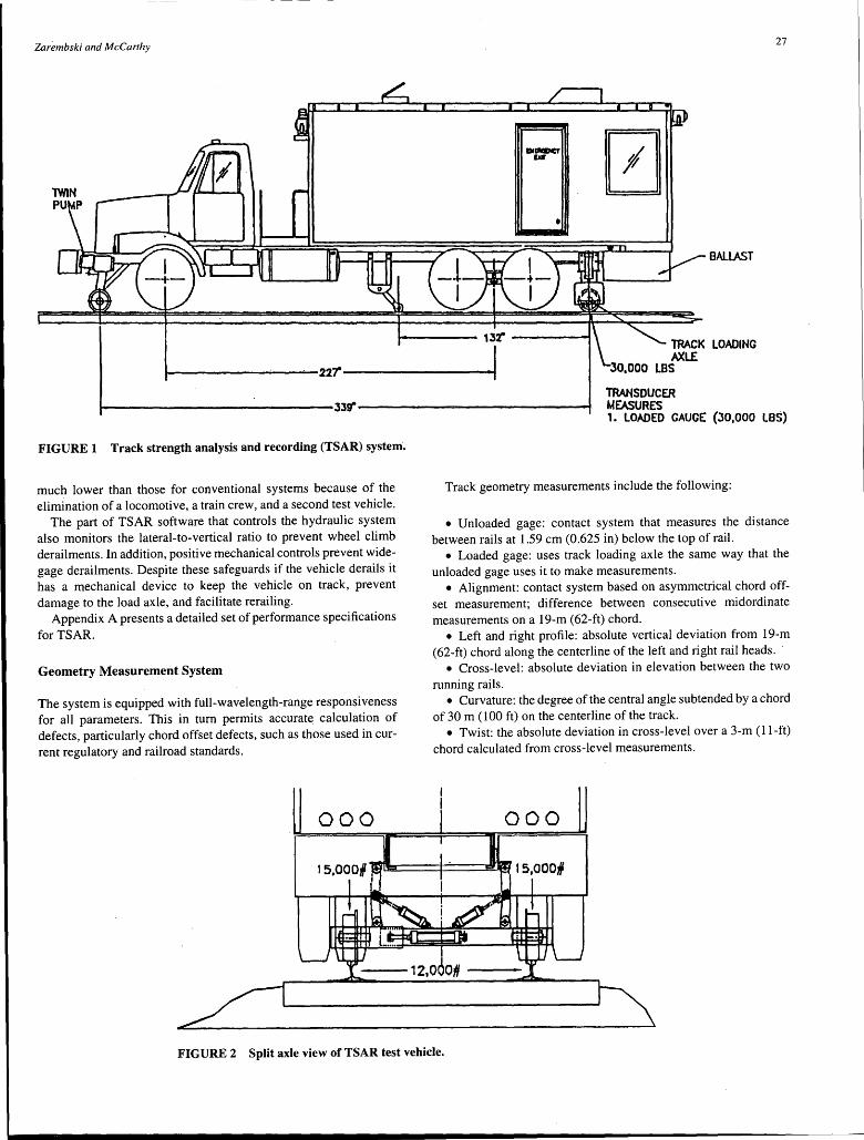
Zarembski and McCarthy 27

• BALLAST

..... ~~~-- 1Jr --~~~--i TRACK LOADING AXLE ---~~~~---~----22~~~~~----~--i·I 30,000 LBS

FIGURE 1 Track strength analysis and recording (TSAR) system.

much lower than those for conventional systems because of the elimination of a locomotive, a train crew, and a second test vehicle.

The part of TSAR software that controls the hydraulic system also monitors the lateral-to-vertical ratio to prevent wheel climb derailments. In addition, positive mechanical controls prevent wide­gage derailments. Despite these safeguards if the vehicle derails it has a mechanical device to keep the vehicle on track, prevent damage to the load axle, and facilitate rerailing.

Appendix A presents a detailed set of performance specifications for TSAR.

Geometry Measurement System

The system is equipped with full-wavelength-range responsiveness for all parameters. This in tum permits accurate calculation of defects, particularly chord offset defects, such as those used in cur­rent regulatory and railroad standards.

000

TRANSDUCER MEASURES 1. LOADED GAUGE (J0,000 LBS)

Track geometry measurements include the following:

• Unloaded gage: contact system that measures the distance between rails at 1.59 cm (0.625 in) below the top of rail.

• Loaded gage: uses track loading axle the same way that the unloaded gage uses it to make measurements.

• Alignment: contact system based on asymmetrical chord off­set measurement; difference between consecutive midordinate measurements on a 19-m (62-ft) chord.

• Left and right profile: absolute vertical deviation from 19-m (62-ft) chord along the centerline of the left and right rail heads.

• Cross-level: absolute deviation in elevation between the two running rails.

• Curvature: the degree of the central angle subtended by a chord of 30 m (100 ft) on the centerline of the track.

• Twist: the absolute deviation in cross-level over a 3-m (11-ft) chord calculated from cross-level measurements.

000

FIGURE 2 Split axle view of TSAR test vehicle.

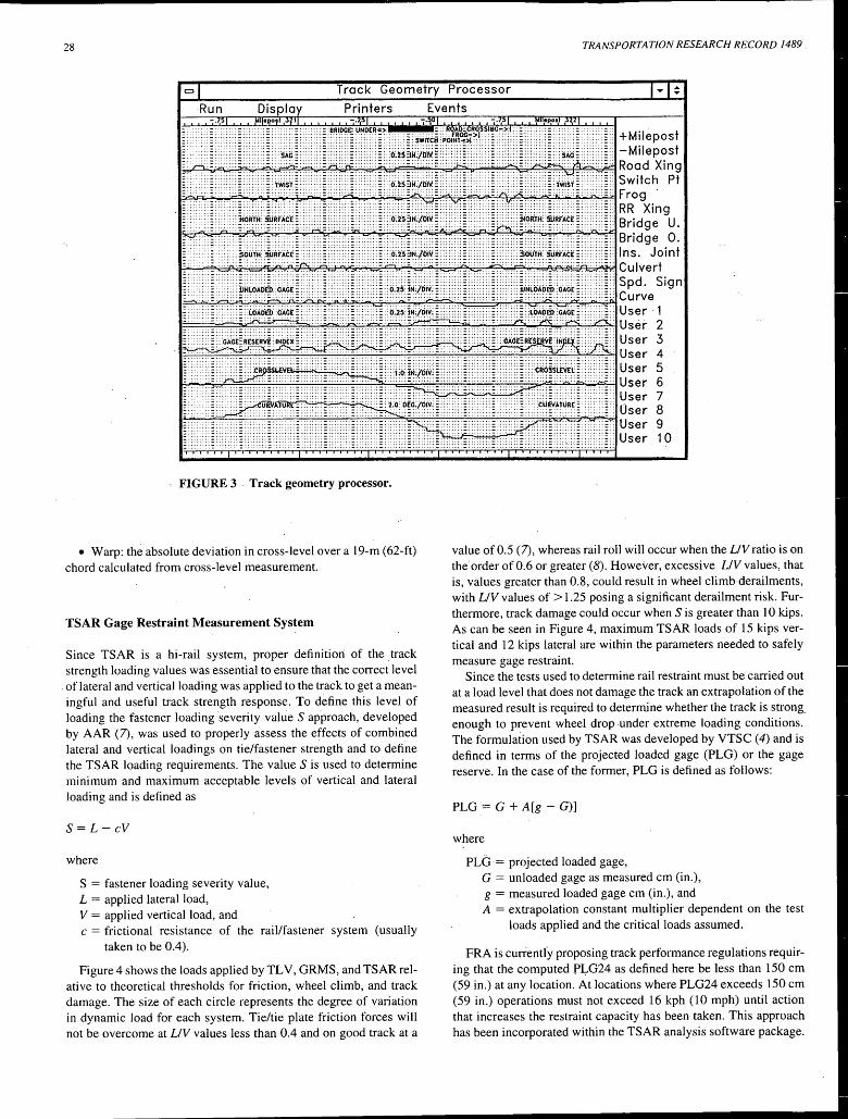
28 TRANSPORTATION RESEARCH RECORD 1489

Track Geometry Processor

Run Printers Events

..... ·- +Milepost -Milepost

ld~~~o.;,;.;..:.;.o.:.~::i::...:.c:::i.:.;.;.:..=~;.;.;.;,;:~~====:;.;..::.;.;,;:,~~====:::::::~~~;.:.:.t.:1~.;.:..=:::1 Road Xing .. ····-·· Switch Pt

... t::rn ~~09xin 9 l5'6~~~~~~~~~~~~.:.:.c::~~~~:;;;p~.:..:;;i.:.;~:.:.;,:;,;;:,;.;.;;,;;.=;,:;,:.o,~Bridge U.

Bridge 0. Ins. Joint

E;.;.;,;,;,;~~r.-:;:~~~~~P.:Y.~~:-g~:.c;.:..:~::::::r.~~~~~~~~t::#""1¥iCulvert Spd. Sign

i==.::.:..:.c;"-?.~~~.:..f=~~~~-J:>.;.:11~.:..<i>-i::::r.;.;~~~=====~~.:.:.:.:..:,:_::,;.;.;.;.;.:.-~~o.;;c:-:-;,;.cc..;.;~:.:.;;.A1Curve User ·1

1;::==:~~~~::::::;::;:::;.:.;.:.:.:.~~~~~~~~~~~~~~~:c:::s.~~user 2 User 3

1=c.'"'-'-'-'="'-'-~='-~.;.::..;..;..;..;.;.;.;~.;_;_;_.;.::..;..;..:.:..:..:..:~;.;...;.;.;.~;_;_;,;_~;.;...;.;.;.;..:;..;.;.;.;.;..;.;.~;.;...;.;.;.~.:.:..:..:..:~.:.:..:..:..:.:.:l:!.:.:..:..:..:~~~user 4

User 5 ~~~~:=:-:-:-:.:.:.:-=-:..:..:.:.:-:~~~.:..:.:.:-:-~~~==:,:.:.:.:.:..:..:.;:.:.:..:.:.:-:-~~~.:.:.:..:..::~,;.;.c;.;.;.:.;:;.;..;;;,>.~~user 6

User 7 _ - ··- Oser 8 •~~~_==::=::::-=-:-:~~~~.:.:.:..:..::~~~~~:g::.;.:.:.:.;.;..~~~~~~.:.:.:::;,~~;.=-:.;;,==-=:~User 9

_ . ··- .... _ .. <::=:: ..... :. ,,,:+H~::F:::: ·- ... -·· ..... _ ..... _ ...... ~:: User 10

FIGURE 3 . Track geometry processor.

• Warp: the absolute deviation in cross-level over a 19-m (62-ft) chord calculated from cross-level measurement.

TSAR Gage Restraint Measurement System

Since TSAR is a hi-rail system, proper definition of the track strength loading values was essential to ensure that the correct level

. of lateral and vertical loading was applied to the track to get a mean­ingful and useful track strength response. To define this level of loading the fastener loading severity value S approach, developed by AAR (7), was used to properly assess the effects of combined lateral and vertical loadings on tie/fastener strength and to define the TSAR loading requirements. The value S is used to determine minimum and maximum acceptable levels of vertical and lateral loading and is defined as

S = L - cV

where

S = fastener loading severity value, L = applied lateral load, V = applied vertical load, and c = frictional resistance of the rail/fastener system (usually

taken to be 0.4).

Figure 4 shows the loads applied by TLV, GRMS; and TSAR rel­ative to theoretical thresholds for friction, wheel climb, and track damage. The size of each circle represents the degree of variation in dynamic load for each system. Tie/tie plate friction forces will not be overcome at LIV values less than 0.4 and on good track at a

value of 0.5 (7), whereas rail roll will occur when the LIV ratio is on the· order of 0.6 or greater (8). However, excessive LIV values, that is, values greater than 0.8, could result in wheel climb derailments, with LIV values of > 1.25 posing a significant derailment risk. Fur­thermore, track damage could occur when Sis greater than 10 kips. As can be seen in Figure 4, maximum TSAR loads of 15 kips ver­tical and 12 kips lateral are within the parameters needed to safely measure gage restraint.

Since the tests used to determine rail restraint must be carried out at a load level that does not damage the track an extrapolation of the measured result is required to determine whether the track is strong_ enough to prevent wheel drop under extreme loading conditions. The formulation used by TSAR was developed by VTSC (4) and is defined in terms of the projected loaded gage (PLG) or the gage reserve. In the case of the former, PLG is defined as follows:

PLG = G + A [g - G)]

where

PLG · = projected loaded gage, G = unloaded gage as measured cm (in.), g = measured loaded gage cm (in.), and A = extrapolation constant multiplier dependent on the test

loads applied and the critical loads assumed.

FRA is currentiy proposing track performance regulations requir­ing that the computed PLG24 as defined here be less than 150 cm (59 in.) at any location. At locations where PLG24 exceeds 150 cm (59 in.) operations must not exceed 16 kph (10 mph) until action that increases the restraint capacity has been taken. This approach has been incorporated within the TSAR analysis software package.

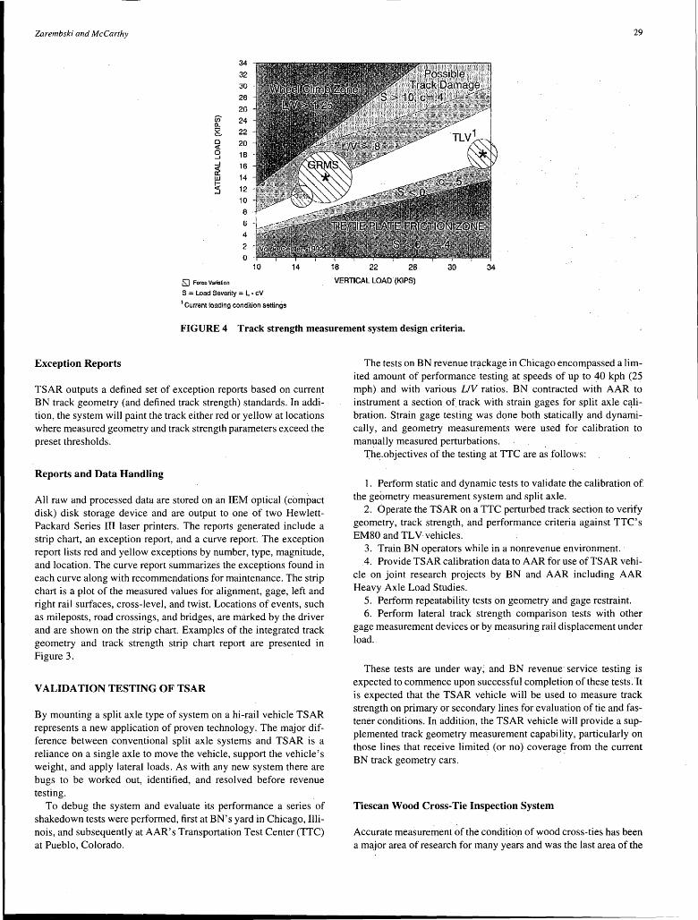
'Zarembski and McCarthy 29

34

32 30

28 -

20 (j} 24 -0... g 22 0 20 -<( 0 18 __J

__J 16 ~ w f4 t-=:5 12

10

8 6 -

4

2

0

ISJ Force Vori:tticn VERTICAL LOAD .(KIPS)

s ; Load Seventy "' L • cv 1 Current loading condillon settings

FIGURE 4 Track strength measurement system design criteria.

Exception Reports

TSAR outputs a defined set of exception reports based on current BN track geometry (and defined track strength) standards. In addi­tion, the system will paint the track either red or yellow at locations where measured geometry and track strength parameters exceed the preset thresholds.

Reports and Data Handling

All raw and processed data are stored on an IEM optical (compact disk) disk storage device and are output to one of two Hewlett­Packard Series III laser printers. The reports generated include a strip chart, an exception report, and a curve report: The exception report lists red and yellow exceptions by number, type, magnitude, and location. The curve report summarizes the exceptions found in each curve along with recommendations for maintenance. The strip chart is a plot of the measured values for alignment, gage, left and right rail surfaces, cross-level, and twist. Locations of events, such as mileposts, road crossings, and bridges, are marked by the driver and are shown on the strip chart. Examples of the integrated track geometry and track strength strip chart report are presented in Figure 3.

VALIDATION TESTING OF TSAR

By mounting a split axle type of system on a hi-rail vehicle TSAR represents a new application of proven technology. The major dif­ference between conventional split axle systems and TSAR is a reliance on a single axle to move the vehicle, support the vehicle's weight, and apply lateral loads. As with any new system there are bugs to be worked out, identified, and resolved before revenue testing.

To debug the system and evaluate its performance a series of shakedown tests were performed, first at BN's yard in Chicago, Illi­nois, and subsequently at AAR's Transportation Test Center (TTC) at Pueblo, Colorado.

The tests on BN revenue tr~ckage in Chicago encompassed a lim­ited amount of performance testing at speeds of up to 40 kph (25 mph) and with various LIV ratios. BN contracted with AAR to instrument a section of track with strain gages for split axle c~Ii­bration. Strain gage testing was done both statically and dynami­cally, and geometry measurements were used for calibration to manually measured perturbations.

The.objectives of the testing at TIC are as follows:

I. Perform static and dynamic tests to validate the calibration of the geometry measurement system and split axle.

2. Operate the TSAR on a TTC perturbed track section to verify geometry, track strength, and performance criteria against TTC's EM80 and TL V vehicles.

3. Train BN operators while in a nonrevenue environment. 4. Provide TSAR calibration data to AAR for use of TSAR vehi­

cle on joint research projects by BN and AAR including AAR Heavy Axle Load Studies.

5. Perform repeatability tests on geometry and gage restraint. 6. Perform lateral track strength comparison tests with other

gage measurement devices or by measuring rail displacement under load.

These tests are under way~ and BN revenue service testing is expected to commence upon successful completion of these tests. It is expected that the TSAR vehicle will be used to measure track strength on primary or secondary lines for evaluation of tie and fas­tener conditions. In addition, the TSAR vehicle will provide a sup­plemented track geometry measurement capability, particularly on those lines that receive limite<;l (or no) coverage from the current BN track geometry cars.

Tiescan Wood Cross-Tie Inspection System

Accurate measurement of the conditio.n of wood cross-ties has been a major area of research for many years and was the last area of the

------------------------------------------------------ - ------

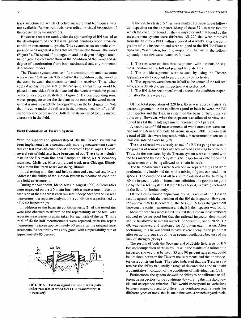
30

track structure for which effective measurement techniques were not available. Rather, railroads have relied on visual inspection of the cross-ties by tie inspectors.

However, recent research under the sponsorship of BN has led to the development of the Tiescan (patent pending) wood cross-tie condition measurement systein. This system relies on sonic com­pression and tangential waves that are transmitted through the wood (Figure 5). The speed of propagation and the degree of signal atten­uation give a direct indication of the condition of the wood and its degree of deterioration from both mechanical and environmental degradation modes.

The Tiescan system consists of a transmitter unit and a separate receiver unit that are used to measure the condition of the wood in the zone between the transmitter and the receiver. Thus, when applied across the rail seat of the cross-tie a transmitter would be placed on one side of the tie plate and the receiver would be placed on the other side, as illustrated in Figure 5. The corres'ponding sonic waves propagate under the tie plate in the zone of the wood mater­ial that is most susceptible to degradation in the tie (Figure 5). Note that this zone under the rail seat is the primary location of tie fail­ure for in-service cross-ties. Both rail seats are tested to fully inspect a cross-tie in the field.

Field Evaluation of Tiescan System

With the support and sponsorship of BN the Tiescan system has been implemented as a continuously moving measurement system that can test cross-tie condition at a speed of 3 kph (2 mph). To date, several sets of field tests have been carried out. These have included tests on the BN main line near Sandpoint, Idaho, a BN secondary main near McBride, Missouri, a yard track near Chicago, Illinois, and a main line track near Galesburg, Illinois.

·Initial testing with the hand-held system and a manual test fixture addressed the ability of the Tiescan system to measure tie condition in a field environment.

During the Sandpoint, Idaho, tests in August 1990, 220 cross-ties were inspected on the BN main line, with a measurement taken on each side of the tie across each rail seat. Independent of the Tiescan measurement, a separate analysis of tie condition was performed by a BN tie inspector (9).

In addition to the basic tie condition tests, 21 of the tested ties were also checked to determine the repeatability of the test, with separate measurements again taken for each side of the tie. Thus, a total of 42 tie half measurements were repeated, with the repeat measurements taken approximately 30 min after the original mea­surements. Repeatability was very good, with a repeatability rate of approximately 85 percent.

·T R

FIGURE 5 Tiescan signal and sonic wave path under rail seat of wood ties (T = transmitter; R = receiver).

TRANSPORTATION RESEARCH RECORD 1489

Of the 220 ties tested, 57 ties were marked for subsequent follow­up inspection (at the tie plant). Many of these 57 ties were ties for which the condition found by the tie inspector and that found by the measurement system were different. All 220 ties were removed from the field by a P811 within a period of 4 weeks after the com­pletion of this inspection and were shipped to the BN Tie Plant at Spokane, Washington, for follow-up study. As part of the follow­up study these ties were treated as follows:

1. The ties were cut into three segments, with the outside seg­ments containing the full rail seat and tie plate area.

2. The outside segments were retested by using the Tiescan apparatus with a couplant to ensure sonic connectivity.

3. The segments were then cut in half at the center of the rail seat area, and a detailed visual inspection was performed.

4. The BN tie inspector performed a second tie condition inspec­. ti on after the ties were cut.

Of the total population of 220 ties, there was approximately 82 percent agreement on tie condition (good or bad) between the BN tie inspector and the Tiescan system on the basis of field observa­tions only. However, when the inspector was allowed to view sec­tioned ties (at the plant) agreement increased to 93 percent.

A second set of field measurements of wood cross-ties were car­ried out on BN near McBride, Missouri, in April 1991. In these tests a total of 201 ties were inspected, with a measurement taken on at least one side of every tie (10).

The site selected was directly ahead of a BN tie gang that was in the process of removing ties already marked as having to come out. Thus, the ties measured by the Tiescan system were compared with the ties marked by the BN system's tie inspector as either requiring replacement or as being allowed to remain in track.

The tie measurements were taken on two separate sites and were . predominantly hardwood ties with a mixing of gum, oak, and other species. The conditions of all ties were evaluated in the field by a BN tie inspector, with an immediate definition of a good_or no good tie by the Tiescan system. Of the 201 ties tested, five were sectioned in the field for further study.

Of the ties evaluated approximately 90 percent of the Tiescan results agreed with the decision of the BN tie inspector. However, for approximately 8 percent of the ties (or 15 ties) disagreement between the sonic measurement and the BN tie inspector was found.

Most of these ties represented ties that the Tiescan measurements showed to be no good but that the railroad inspector determined should be allowed to remain in track. For example, one such tie, Tie 69, was removed and sectioned for follow-up examination. After sectioning, this tie was found to have severe decay to the point that after sectioning, one side of the tie segment collapsed because of the lack of strength (decay).

The results of both the Spokane and McBride field tests of BN ties and comparison of those results with the results of a railroad tie inspector showed that between 85 and 90 percent agreement could be obtained between the Tiescan measurements and the tie inspec­tor on a consistent basis. They also indicated that the Tiescan sys­tem has the ability to quantify a range of tie conditions and to obtain a quantitative indication of the conditions of individual ties (11).

Furthermore, the system showed the ability to be calibrated to dif­ferent tie inspectors (or tie conditions) by varying the threshold lev­els and acceptance criterion. This would correspond to variations between inspectors and to different tie condition requirements for different types of track, that is, main line versus branch or yard track.

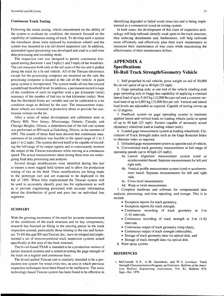
7-arembski and McCarthy

Continuous Track Testing

Following the initial testing, which concentrated on the ability of the system to evaluate tie condition, the research focused on the capability of continuous testing of track. To develop such a system the transducer shoes were replaced by transducer wheels and the system was mounted in a hi-rail drawn inspection cart. In addition, automated signal processing was developed and used in a real-time data processing and recording mode.

The inspection cart was designed to permit continuous low­speed testing (between 1 and 5 kph) ( 1 and 3 mph) of the wood ties. The cart measures both rails at the rail seats of the ties and is pulled along the track by a hi-rail vehicle. All of the Tiescan electronics except for the processing computer are mounted on the cart; the processing computer is located in the cab of the vehicle. A paint spray system is incorporated. The system marks all ties that exceed a predefined threshold level. In addition, a permanent record is kept of the condition of each tie together with a per kilometer (mile) summary of the number of bad ties in that kilometer (mile). Note that the threshold limits are variable and can be calibrated to a tie condition range as defined by the user. The measurement trans­ducer wheels are mounted in protective shoes to provide for con­tinuous contact on the tie.

After a series of initial development and calibration tests in Cherry Hill, New Jersey; Mississauga, Ontario, Canada; and Chicago Heights, Illinois, a shakedown test of the full cart system was performed on BN track at Galesburg, Illinois, in the summer of 1993. The results of those field tests showed that continuous mea­surement of tie condition was feasible in the speed range of 1 to 3 kph (1to2 mph). The system showed itself to be capable ofrecord­ing the full range of tie output signals and to continuously monitor the output of the Tiescan transducers while moving at a continuous speed. The actual measurements taken during these tests are under­going final data processing and analysis.

Several design modifications were identified during this test to ensure a more rugged field system and to allow for production testing of ties in the field. These modifications are being made to the prototype cart and are expected to be deployed in the fall of 1995. When fully implemented the Tiescan system will be used to accurately identify poor ties for replacement as well as to provide engineering personnel. with accurate information about the distribution of good and poor ties on individual line segments.

SUMMARY

With the growing awareness of the need for accurate measurement of the conditions of the track structure and its key components, research has focused on filling in the missing pieces in the track inspection arsenal, particularly those relating to the ties and fasten­ers. To fill this gap BN and Tiescan, Inc., have developed and imple­mented a set of nonconventional track inspection systems aimed specifically at this area of the track structure.

The hi-rail-based TSAR is intended to be a production version of earlier research systems and is aimed at testing the gage strength of the track on a regular and continuous basis.

The hi-rail-pulled Tiescan cart is similarly intended to be a pro­duction test system for wood cross-ties, an area in which previous inspection techniques have been found to be ineffective. The sonic . technology-based Tiescan system has been found to be effective in

31

identifying degraded or failed wood cross-ties and is being imple­mented as a commercial wood tie testing system.

In both cases, the development of this class of inspection tech­nology will help railroads identify weak spots in the track structure, thus reducing derailments and, furthermore, will help railroads more efficiently and effectively plan their track maintenance to minimize their maintenance of way costs while maximizing the effectiveness of their maintenance dollars.

APPENDIX A Specifications Hi-Rail Track Strength/Geometry Vehicle

1. Self-propelled hi-rail vehicle; gross weight on rail of 50,000 lbs on rail speed of up to 40 kph (25 mph).

2. Gage spreading axle; at one end of the vehicle (trailing end) gage spreading axle or buggy has capability of applying a constant lateral load ofup to 5,443 kg (12,000 lbs) per rail and a constant ver­tical load of up to 6,803 kg (15,000 lbs) per rail. Vertical and lateral load levels are adjustable as required. Capable of testing curves up to 12 degrees.

3. Feedback system on gage spreading system to maintain applied lateral and vertical loads on loading wheels (axle) at speed of up to 40 kph (25 mph). System capable of necessary actual (dynamic) wheel/rail load at loading wheel (axle).

4. Loaded gage measurement system at loading wheel/axle. Cal­culation of Track Strength Index such as the Gage Restraint Index or alternate index as required.

5. Unloaded gage measurement system at opposite end of vehicle. 6. Conventional track geometry measurements at full range of

operating speeds (up to 40 kph (25 mph)). 6a. Lateral alignment measurement system (cord or

accelerometer) based. Separate measurements for left and right rails.

6b. Vertical profile measurement system (cord or accelerom­eter) based. Separate measurements for left and right rails.

6c. Cross-level measurement. 6d. Warp or twist measurement.

7. Complete hardware and software for computerized data analysis, processing, real-time reporting, and storage. This is to include

• Exception reports for track geometry, • Exception reports for track strength, • Continuous recording of track geometry at 3-m

(1-ft) intervals, • Continuous recording of track strength at 3-m (1-ft)

intervals, • Continuous output of track geometry (strip chart), • Continuous output of track strength (selectable), • Storage of track geometry data via optical disk, and • Storage of track strength data via optical disk.

8. Paint spray system.

REFERENCES

1. McConnell, D. P., A. M. Zarembski, and W. S. Lovelace. Track Strength Characterization Program; an Overview. Bulletin of the Amer­ican Railway Engineering Association, Vol. 81, Bulletin 674, Sept.-Oct. 1979.

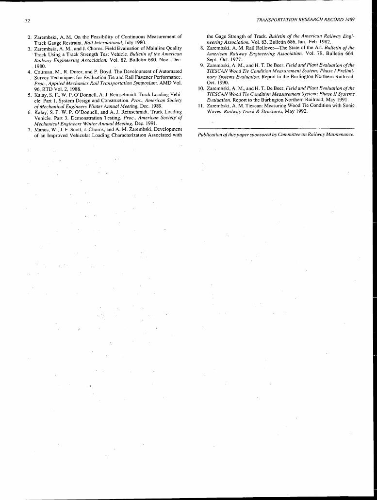
32

2. Zarembski, A. M. On the Feasibility of Continuous Measurement of Track Gauge Restraint. Rail International, July 1980.

3. Zarembski, A. M., and J. Choros. Field Evaluation of Mainline Quality · Track Using a Track Strength Test Vehicle. Bulletin of the American Railway Engineering Association, Vol. 82, Bulletin 680, Nov.-Dec.

. 1980. 4. Coltman, M., R. Dorer, and P. Boyd. The Development of Automated

Survey Techniques for Evaluation Tie and Rail Fastener Performance. Proc., Applied Mechanics Rail Transportation Symposium, AMD Vol. 96, RTD Vol. 2, 1988.

5. Kalay, S. F., W. P. O'Donnell, A. J. Reinschmidt. Track Loading Vehi­cle. Part 1. System Design and Construction. Proc., America_n Society of Mechanical Engineers Winter Annual Meeting, Dec. 1989.

6. Kalay; S. F. W. P. O'Donnell, and A. J. Reinschmidt. Track Loading Vehicle. Part 3. Demonstration Testing. Proc., American Society of Mechanical Engineers Winter Annual Meeting, Dec. 1991.

7. Manos, W., J. F. Scott, J. Choros, and A. M. Zarembski. Development of an Improved Vehicular Loading Characterization Associated with

TRANSPORTATION RESEARCH RECORD 1489

the Gage Strength of Track. Bulletin of the American Railway Engi­neering Association, Vol. 83, Bulletin 686, Jan.-Feb. 1982.

8. Zarembski, A. M. Rail Rollover-The State of the Art. Bulletin of the American Railway Engineering Association, Vol. 79, Bulletin 664, Sept.-Oct. 1977.

9. Zarembski, A. M., and H. T. De Beer. Field and Plant Evaluation of the TIESCAN Wood Tie Condition Measurement System; Phase I Prelimi­nary Systems Evaluation. Report to the Burlington Northern Railroad, Oct. 1990.

I 0. Zarembski, A. M., and H. T. De Beer. Field and Plant Evaluation of the TIESCAN Wood Tie Condition Measurement System; Phase II Systems Evaluation. Report to the Burlington Northern Railroad, May 1991.

11. Zarembski, A. M. Tiescan: Measuring Wood Tie Condition with Sonic Waves. Railway Track & Structures, May 1992.

Publication of this paper sponsored by Committee on Railway Maintenance.

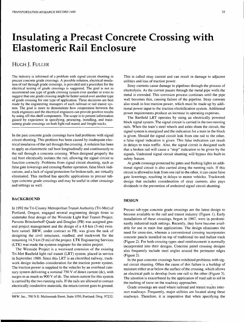
TRANSPORTATION RESEARCH RECORD 1489 33

Insulating a Precast Conc~ete Crossing with Elastomeric Rail Enclosure

HUGH J. FULLER

The industry is informed of a problem with signal circuit shunting in precast concrete grade crossings. A possible solution, electrical insula­tion of rail through grade crossings, is provided and a procedure for the electrical testing of grade crossings is suggested. The· goal is not to recommend one type of grade crossing system over another or even to suggest that one grade crossing might be better suited over another type of grade crossing for one type of application. These decisions are best made by the engineering managers of each railroad or rail transit sys­tem. The goal is more to demonstrate how cooperation between the track engineers and the electrical engineers can provide positive results by using off-the-shelf components. The scope is to present information gained by experience in specifying, procuring, installing, and main­taining grade crossings on both light rail transit and freight tracks.

In the past concrete grade crossings have had problems with signal circuit shunting. This problem has been caused by inadequate elec­trical insulation of the rail through the crossing. A solution has been to apply an elastomeric rail boot longitudinally and continuously to the rail through a concrete crossing. When designed properly the rail boot electrically isolates the rail, allowing the signal circuit to function correctly. Problems from signal circuit shunting, such as false gate lowerings and crossing flasher operation, false block indi­cations, and a lack of signal protection for broken rails, are virtually eliminated. This method has specific applications to precast tub­type concrete grade crossings and may be useful in other crossings and settings as well. ·

BACKGROUND

In 1992 the Tri-County Metropolitan Transit Authority (Tri-Met) of Portland, Oregon, engaged several engineering design firms to undertake final design of the Westside Light Rail Transit Project. Parsons Brinckerhoff Quade and Douglas (PB) was assigned gen­eral project management and the design of a 4.8-km (3-mi) twin­bore tunnel. BRW, under contract to PB, ·was given the task of designing the civil struc;tures, roadbed, and trackwork for the remaining 14.5 km (9 mi) of the. project. LTK Engineering Services (LTK) was made the systems enginyer for the entire project.

The Westside Project is a westward extension of the existing Tri-Met Banfield light rail transit (LRT) system, placed in service in September 1986. Since this LRT is an electrified railway, track­work design includes consideration for the traction power system. The traction power is supplied to the vehicles by an overhead cate­nary system delivering a nominal 750 V of direct current (de), with surges to as much as 900 V of de. The return current for this system is carried by the two running rails. If the rails are allowed to contact electrically conductive materials, the return current goes to ground.

BRW, Inc., 700 N.E. Multnomah Street, Suite 1050, Portland, Oreg. 97232.

This is called stray current and can result in damage to adjacent utilities and loss of traction power.

Stray currents cause damage to pipelines through the process of electrolysis. As the current passes through the metal pipe walls the metal is corroded. This corrosion process continues until the pipe wall becomes thin, causing failure of the pipeline. Stray currents also result in lost traction power, which must be made up by addi­tional power input to the traction electrification system. Additional power requirements produce an increase in operating expenses.

The Banfield LRT operates by using an electrically powered block signal system. The signal circuit is carried in the two running rails. When the train's steel wheels and axles shunt the circuit, the signal system is energized and the indication for a train in the block is given. Should the signal circuit leak from one rail to the other, a false signal indication is given. This false indication can result in delays to train traffic. Also, the signal circuit is designed such that a broken rail will cause a "stop" indication to be given by the signals. Undesired signal circuit shunting will bypass this built-in safety feature.

At grade crossings protected by gates and flashing lights an addi­tional signal circuit is also carried along the running rails. If this circuit is allowed to leak from one rail to the other, it can cause false gate lowerings, resulting in delays to motor vehicles. Trackwork design that includes consideration of stray currents also pays dividends in the prevention of undesired signal circuit shunting.

DESIGN

Precast tub-type concrete grade crossings are the latest design to become available to the rail .and transit industry (Figure 1). Early installations of these crossings, begun in 1967, were in predomi­nantly industrial track settings. Recently, they have become avail­able for use in main line applications. The design eliminates the need for cross-ties, whereas a conventional crossing incorporates concrete panels installed on top of traditional tie-and-ballast track (Figure 2). For both crossing types steel reinforcemeri.t is normally inc.9rporated into their designs. Concrete panel crossing designs also frequently include steel angles around the perimeter edges (Figure 2).

In the past concrete crossings have exhibited problems with sig­nal circuit shunting. Often the caus.e of this· failure is a buildup of moisture either at or below the surface of the crossing, which allows an electrical path to develop from one rail to the other (Figure 3). The situation is exacerbated by the application of rqad salt to aid in the· melting of snow on the roadway approaches.

Grade crossings are used where railroad and tran,sit tracks inter­sect roadways. Frequently, major utilities are located along these roadways. Therefore, it is imperative that when specifying the

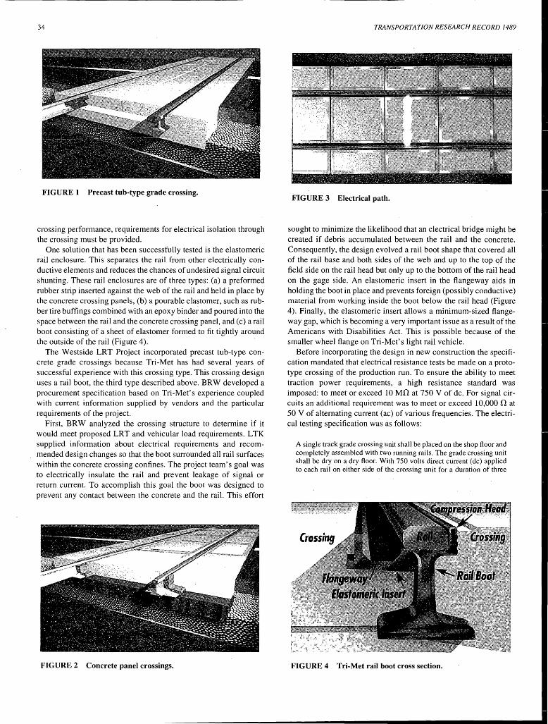
34

FIGURE 1 Precast tub-type grade crossing.

crossing performance, requirements for electrical isolation through the crossing must be provided.

One so'Jution that has been successfully tested is the elastomeric rail enclosure. This separates the rail from other electrically con­ductive elements and reduces the chances of undesired signal circuit shunting. These rail enclosures are of three types: (a) a preformed rubber strip inserted against the web of the rail and held in place by the concrete crossing panels, (b) a pourable elastomer, such as rub­ber tire buffings combined with an epoxy binder and poured into the space between the rail and the concrete crossing panel, and (c) a rail boot consisting of a sheet of elastomer formed to fit tightly around the outside of the rail (Figure 4).

The Westside LRT Project incorporated precast tub-type con­crete grade crossings because Tri-Met has had several years of successful experience with this crossing type. This crossing design uses a rail boot, the third type described above. BRW developed a procurement specification based on Tri-Met's experience coupled with current information supplied by vendors and the particular requirements of the project.

First, BRW analyzed the crossing structure to determine if it would meet proposed LRT and vehicular load requirements. LTK supplied information about electrical requirements and recom­mended design changes so that the boot surrounded all rail surfaces within the concrete crossing confines. The project team's goal was to electrically insulate the rail and prevent leakage of signal or return current. To accomplish this goal the boot was designed to prevent any contact between the concrete and the rail. This effort

FIGURE 2 Concrete panel crossings.

TRANSPORTATION RESEARCH RECORD 1489

FIGURE 3 Electrical path.

sought to minimize the likelihood that an electrical bridge might be created if debris accumulated between .the rail and the concrete. Consequently, the design evolved a rail boot shape that covered all of the rail base and both sides of the web and up to the top of the field side on the rail head but only up to the.bottom of the rail head on the gage side. An elastomeric insert in the ftangeway aids in holding the boot in place and prevents foreign (possibly conductive) material from working inside the boot below the rail head (Figure 4). Finally, the elastomeric insert allows a minimum-sized ftange­way gap, which is becoming a very important issue as a result of the Americans with Disabilities Act. This is possible because of the smaller wheel flange on Tri-Met's light rail vehicle.

Before incorporating the design in new construction the specifi­cation mandated that electrical resistance tests be made on a proto­type crossing of the production run. To ensure the ability to meet traction power requirements, a high resistance standard was imposed: to meet or exceed 10 MD at 750 V of de. For signal cir­cuits an additional requirement was to meet or exceed 10,000 n. at 50 V of alternating current (ac) of various frequencies. The electri­cal testing specification was as follows:

A single track grade crossing unit shall be placed on the shop floor and completely assembled with two running rails. The grade crossing unit shall be dry on a dry floor. With 750 volts direct current (de) applied to each rail on either side of the crossing unit for a duration of three

FIGURE 4 Tri-Met rail boot cross section.

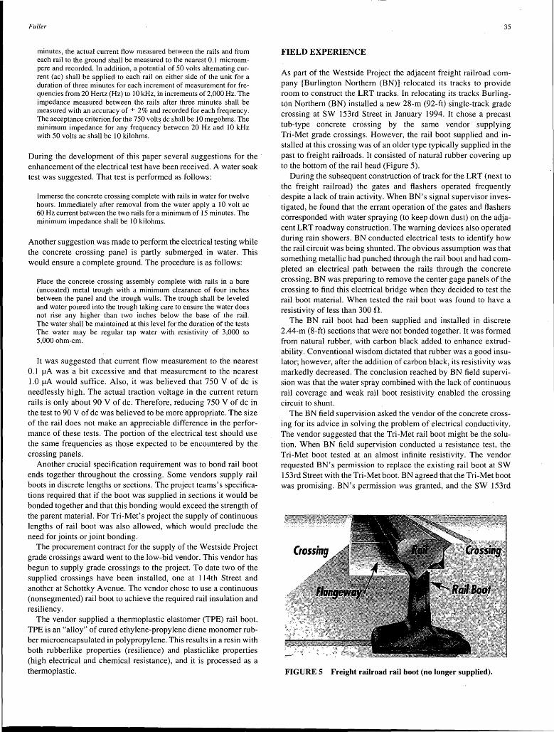
Fuller

minutes, the actual current flow measured between the rails and from each rail to the ground shall be measured to the nearest 0.1 microam­pere and recorded. In addition, a potential of 50 volts alternating cur­rent (ac) shall be applied to each rail on either side of the unit for a duration of three minutes for each increment of measurement for fre­quencies from 20 Hertz (Hz) to 10 kHz, in increments of 2,000 Hz. The impedance measured between the rails after three minutes shall be measured with an accuracy of:±: 2% and recorded for each frequency. The acceptance criterion for the 750 volts de shall be 10 megohms. The minimum impedance for any frequency between 20 Hz and IO kHz with 50 volts ac shall be 10 kilohms.

During the development of this paper several suggestions for the enhancement of the electrical test have been received. A water soak test was suggested. That test is performed as follows:

Immerse the concrete crossing complete with rails in water for twelve hours. Immediately after removal from the water apply a IO volt ac 60 Hz current between the two rails for a minimum of 15 minutes. The minimum impedance shall be 10 kilohms.

Another suggestion was made to perform the electrical testing while the concrete crossing panel is partly submerged in water. This would ensure a complete ground. The procedure is as follows:

Place the concrete crossing assembly complete with rails in a bare (uncoated) metal trough with a minimum clearance of four inches between the panel and the trough walls. The trough shall be leveled and water poured into the trough taking care to ensure the water does not rise any higher than two inches below the base of the rail. The water shall be maintained at this level for the duration of the tests The water may be regular tap water with resistivity of 3,000 to 5,000 ohm-cm.

It was suggested that current flow measurement to the nearest 0.1 µA was a bit excessive and that measurement to the nearest 1.0 µA would suffice. Also, it was believed that 750 V of de is needlessly high. The actual traction voltage in the current return rails is only about 90 V of de. Therefore, reducing 750 V of de in the test to 90 V of de was believed to be more appropriate. The size of the rail does not make an appreciable difference in the perfor­mance of these tests. The portion of the electrical test should use the same frequencies as those expected to be encountered by the crossing panels.

Another crucial specification requirement was to bond rail boot ends together throughout the crossing. Some vendors supply rail boots in discrete lengths or sections. The project teams's specifica­tions required that if the boot was supplied in sections it would be bonded together and that this bonding would exceed the strength of the parent material. For Tri-Met's project the supply of continuous lengths of rail boot was also allowed, which would preclude the need for joints or joint bonding.

The procurement contract for the supply of the Westside Project grade crossings award went to the low-bid vendor. This vendor has begun to supply grade crossings to the project. To date two of the supplied crossings have been installed, one at I 14th Street and another at Schottky A venue. The vendor chose to use a continuous (nonsegmented) rail boot to achieve the required rail insulation and resiliency.

The vendor supplied a thermoplastic elastomer (TPE) rail boot. TPE is an "alloy" of cured ethylene-propylene diene monomer rub­ber microencapsulated in polypropylene. This results in a resin with both rubberlike properties (resilience) and plasticlike properties (high electrical and chemical resistance), and it is processed as a thermoplastic.

35

FIELD EXPERIENCE

As part of the Westside Project the adjacent freight railroad com­pany [Burlington Northern (BN)] relocated its tracks to provide room to construct the LRT tracks. In relocating its tracks Burling­ton Northern (BN) installed a new 28-m (92-ft) single-track grade crossing at SW 153rd Street in January 1994. It chose a precast tub-type concrete crossing by the same vendor supplying Tri-Met grade crossings. However, the rail boot supplied and in­stalled at this crossing was of an older type typically supplied in the past to freight railroads. It consisted of natural rubber covering up to the bottom of the rail head (Figure 5).

During the subsequent construction of track for the LRT (next to the freight railroad) the gates and flashers operated frequently despite a lack of train activity. When BN' s signal supervisor inves­tigated, he found that the errant operation of the gates and flashers corresponded with water spraying (to keep down dust) on the adja­cent LRT roadway construction. The warning devices also operated during rain showers. BN conducted electrical tests to identify how the rail circuit was being shunted. The obvious assumption was that something metallic had punched through the rail boot and had com­pleted an electrical path between the rails through the concrete crossing. BN was preparing to remove the center gage panels of the crossing to find this electrical bridge when they decided to test the rail boot material. When tested the rail boot was found to have a resistivity of less than 300 n.

The BN rail boot had been supplied and installed in discrete 2.44-m (8-ft) sections that were not bonded together. It was formed from natural rubber, with carbon black added to enhance extrud­ability. Conventional wisdom dictated that rubber was a good insu­lator; however, after the addition of carbon black, its resistivity was markedly decreased. The conclusion reached by BN field supervi­sion was that the water spray combined with the lack of continuous rail coverage and weak rail boot resistivity enabled the crossing circuit to shunt.

The BN field supervision asked the vendor of the concrete cross­ing for its advice in solving the problem of electrical conductivity. The vendor suggested that the Tri-Met rail boot might be the solu­tion. When BN field supervision conducted a resistance test, the Tri-Met boot tested at an almost infinite resistivity. The vendor requested BN' s permission to replace the existing rail boot at SW 153rd Street with the Tri-Met boot. BN agreed that the Tri-Met boot was promising. BN's permission was granted, and the SW 153rd

FIGURE 5 Freight railroad rail boot (no longer supplied).

36

Street crossing was retrofitted with the Tri-Met rail boot and the associated elastomeric insert. The consequence of this retrofit is that BN has minimized false gate lowerings. Water truck spraying no longer activates the gates.

The vendor now supplies rubber boot and elastomeric insert meeting the Tri-Met specification as standard equipment on all its crossings.

CONCLUSION

Because of the design process for Tri-Met's Westside LRT Project, a superior form of rail insulation has been identified and applied to

TRANSPORTATION RESEARCH RECORD 1489

precast tub-type concrete grade crossings. This insulator is a con­tinuous rail boot comprising TPE, which isolates the rail from contact with the concrete crossing structure.

Cooperation between the electrical engineers and the track engineers resulted in a solution to a persistent problem. Elec­trical testing of the grade crossing track structure at the procurement stage resulted in a superior product. Actual field experience will determine how well the track engineers have performed their job.

Publication of this paper sponsored by Committee on Railroad Track Structure System Design.

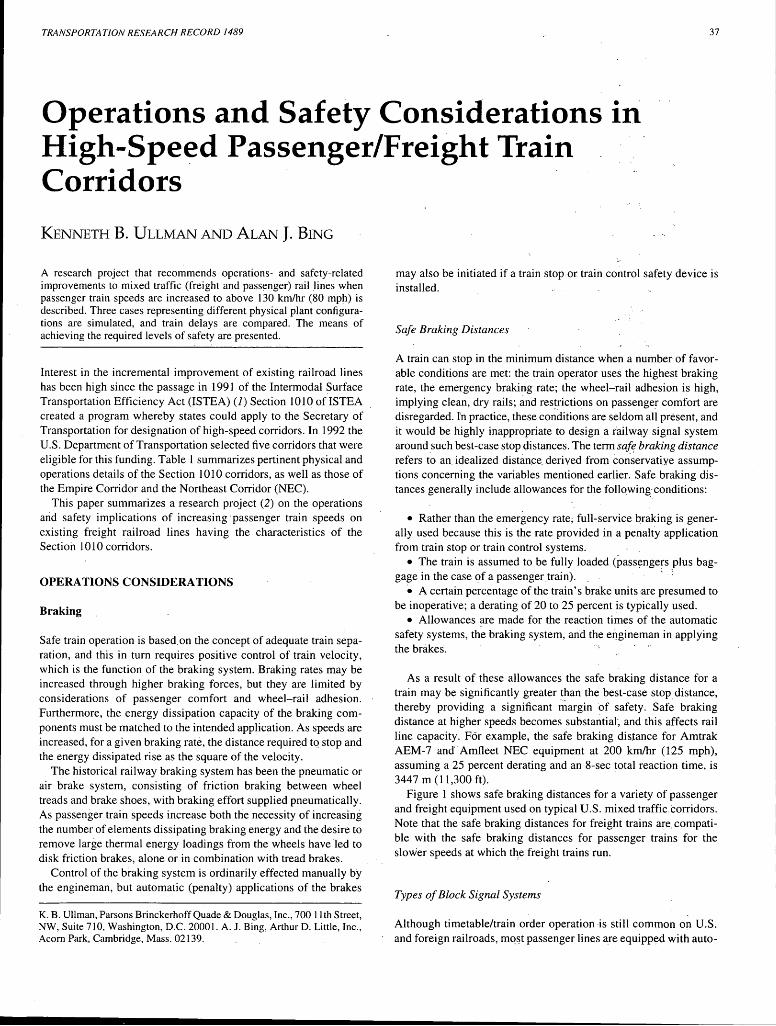
TRANSPORTATION RESEARCH RECORD 1489 37

Operations and Safety Considerations in High-Speed Passenger/Freight Train Corridors

KENNETH B. ULLMAN AND ALAN J. BING

A research project that recommends operations- and safety-related improvements to mixed traffic (freight and passenger) rail lines when passenger train speeds are increased to above 130 km/hr (80 mph) is described. Three cases representing different physical plant configura­tions are simulated, and train delays are compared. The means of achieving the required levels of safety are presented.

Interest in the incremental improvement of existing railroad lines has been high since the passage in 1991 of the Intermodal Surface Transportation Efficiency Act (ISTEA) ( 1) Section 1010 of IS TEA created a program whereby states could apply to the Secretary of Transportation for designation of high-speed corridors. In 1992 the U.S. Department of Transportation selected five corridors that were eligible for this funding. Table 1 summarizes pertinent physical and operations details of the Section 1010 corridors, as well as those of the Empire Corridor and the Northeast Corridor (NEC).

This paper summarizes a research project (2) on the operations arid safety implications of increasing passenger train speeds on existing freight railroad lines having the characteristics of the Section 1010 corridors.

OPERATIONS CONSIDERATIONS

Braking

Safe train operation is based. on the concept of adequate train sepa­ration, and this in turn requires positive control of train velocity, which is the function of the braking system. Braking rates may be increased through higher braking forces, but they are limited by considerations of passenger comfort and wheel-rail adhesion. Furthermore, the energy dissipation capacity of the braking com­ponents must be matched to the intended application. As speeds are increased, for a given braking rate, the distance required tQ stop and the energy dissipated rise as the square of the velocity.

The historical railway braking system has been the pneumatic or air brake system, consisting of friction braking between wheel treads and brake shoes, with braking effort supplied pneumatically. As passenger train speeds increase both the necessity of increasing the number of elements dissipating braking energy and the desire to remove large thermal energy loadings from the wheels have led to disk friction brakes, alone or in combination with tread brakes.

Control of the braking system is ordinarily effected manually by the engineman, but automatic (penalty) applications of the brakes

K. B. Ullman, Parsons Brinckerhoff Quade & Douglas, Inc., 700 11th Street, NW, Suite 710, Washington, D.C. 20001. A. J. Bing, Arthur D. Little, Inc., Acorn Park, Cambridge, Mass. 02139.

may also be initiated if a train stop or train control safety device is installed.

Safe Braking Distances

A train can stop in the minimum distance when a number· of favor­able conditions are met: the train operator uses the highest braking rate, the emergency braking rate; the wheel-rail adhesion is high, implying clean, dry rails; and res~rictions on passenger comfort are disregarded. In practice, these conditions are seldom all present, and it would be highly inappropriate to design a railway signal system around such best-case stop distances. The term saff! braking distance refers to an idealized distance. derived from conservatiye assump­tions concerning the variables mentioned earlier. Safe braking dis­tances generally include allowances for the following,-conditions:

• Rather than the emergency rate; full-service braking is gener­ally used because this is the rate provided in a penalty application from train stop or train control systems.

• The train is assumed to be fully loaded (passengers _plus bag-gage in the case ()fa passenger train). _ ·

e A certain percentage of the train's brake units are presumed to be inoperative; a derating of 20 to 25 percent is typically used.

• Allowances are made for the reaction times of the automatic safety systems, the braking system, and the en.gineman in applying the brakes.

As a result of these allowances the safe braking distance for a train may be significantly greater than the best-case stop distance, thereby providing a significant ~argin of safety. Saf~ braking distance at higher speeds becomes substantial, and this affects rail line capacity. For example, the safe braking distance for Amtrak AEM-7 and Amfteet NEC equipment at 200 km/hr (125 mph), assuming a 25 percent derating and an 8-sec total reaction time, is 3447 m (11,300 ft).

Figure 1 shows safe braking distances for a variety of passenger and freight equipment used on typical U.S. mixed traffic corridors. Note that the safe braking distances for freight trains are. compati­ble with the safe braking distances for passenger trains for the slower speeds at which the freight trains run.

Types of Block Signal Systems

Although timetable/train order operation is still common on U.S. and foreign railroads, mq~t passenger lines are equipped with auto-

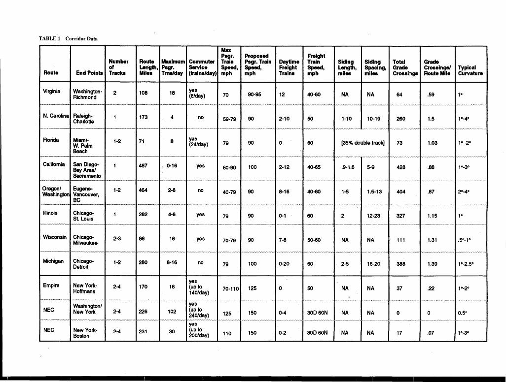
TABLE 1 Corridor Data

Number of

Route End Points Tracks

Virginia

N. Carolina

.. ,,.... ... ..,_~---

Florida

Washington­Richmond

Raleigh-Charlotte

y_. __ .,...,_,,,,.,.,.,,_,...,.,_,...,..

Miami-W. Palm Beach

Califomia San Diego­Bay Area/ Sacramento

Oregon/ Eugene-Washington Vancouver,

BC

Illinois Chicago­Sl Louis

Wisconsin Chicago-

Michigan

Empire

.,........,_,,,...,,....,.,,,,.,,'W.W-W•V..,,,..,,,.

NEC

Milwaukee

Chicago-Detroit

New York-Hoffmans

"\.-.w,<wM-•A.;,.,.,,,.,,,..........,_RYfMW,.,,...H'"'

Washington/ New York

2

_._._,,.,,.....,_....,_,w_. ... w_...,.,..,,....,

1-2

1-2

2-3

1-2

2-4

2-4

Max Pagr. Proposed

Route Maximum Commuter Train Pagr. Train ·Daytime Length, Pagr. Service Speed, Speed, Freight Miles Trne/day (trains/day) mph mph Traina

108 18

173 4

y,w,.,,,,..,.,..,. .. ,.,.,~,~·- .................... .,,.,., ... .,,.,.,,.,....,...,......,., ... , ......

71 8

487 0-16

464 2-8

282 4-8

86 16

280 8-16

170 1S

....... ,.,. ... ,.,.,,,..,,,,..Y,...,,.,...,,.,,.,.,,,,,

22S 102

yes (8/day)

no

yes (24/day)

yes

no

yes

yes

no

yes (up to 140/day)

•vww .. .,,,,..,,,,..,,.,w·,.,..,,,--.•,.,......,.,.,..,_,...,,.,,,

yes (up to 240/day)

70 90-95 12

59-79 90 2-10

, .... , .. ,.,.w,..,...,_.,,,...,,.,,,._,,.,,.,

79 90 0

60-90 100 2-12

40-79 90 8-1S

79 90 0-1

70-79 90 7-8

79 100 0-20

70-110 125 0

•v.·;v.-. .-,,,.,,,...,,,w,,.,,Aww•e.w

125 150 0-4

Freight Train Speed, mph

40-60

50

60

40-65

40-60

60

50-60

60

50

300 SON

Siding Length, miles

NA

1-10

Siding Total Grade Spacing, Grade Crossings/ Typical miles Crossings Route Mile Curvature

NA 64 .59

10-19 260 1.5

[35% double track) 73 1.03

.9-1.6 5-9 428 .88

1-5 1.5-13 404 .87

2 12-23 327 1.15

NA NA 111 1.31

2-5 1S-20 388 1.39

NA NA 37 .22

NA NA 0 0 0.5° __ .,_,,·--·•- •--·----··---"~"- v-N.W""-"--w·w--.w- ~·--·--- ""--"·w,,_.,, __ , __ ,,,__'""'"'""""'"""'""'-'-·'" ""'"~'''""'·'-"''""" '"'""'"""""'-"'"·M~---·~"'""[-••·''"""·""·'"'""''"'"-:'"-""·""" ___ '""'"""""'"""""l""'"''""""'"·'""'"•''°"'""""""'l""""""""""·""···•·"""""'""-':·"""'"'""""'"''""'"""'""'""'"""";·-"""""'·'"""""""'""""""""·"""'""''""l""''"""''""•·"'""""'"""··""""""""""""'I

NEC New York­Boston

2-4 231 30

yes (up to 200/day) 110 150 0-2 300 SON NA NA 17 .07

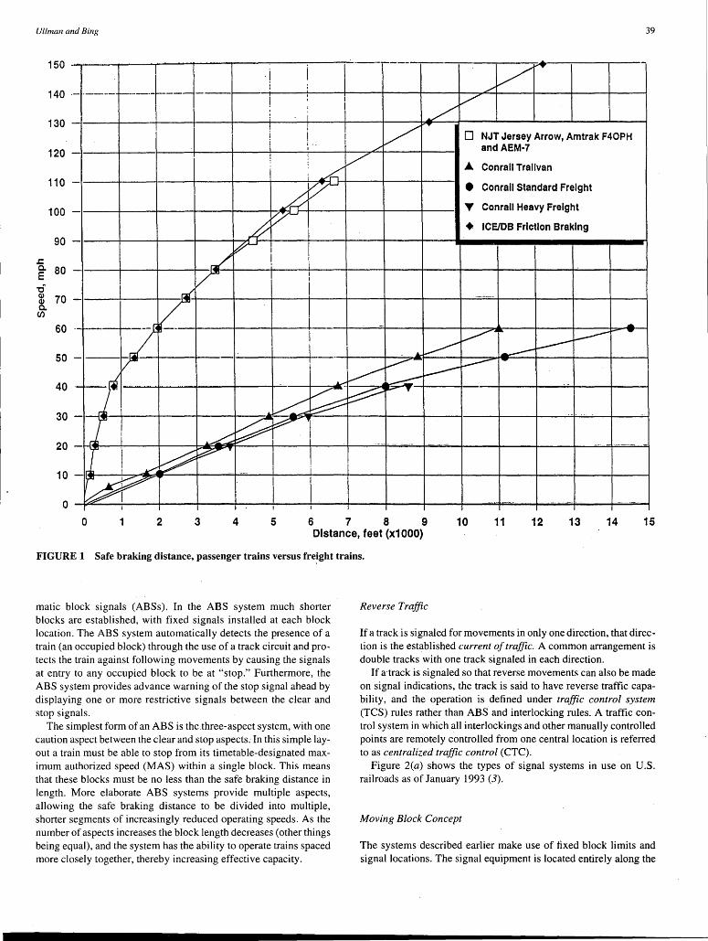
Ullman and Bing 39

150

140

130

---·----- . -I v ..-T

/ ·- ·---- ~--·--·- i------ : I / i \ ./ r l /~ I

0 I I NJT Jersey Arrow, Amtrak F40PH I·- I

/ and AEM·7 I

120 ! / :~ .A Conrail Trallvan

110

100

lv • Conrail Standard Freight

~ 'Y Conrail Heavy Freight V"'

90

.c: c. 80 E -0 <l> 70 Cl> c. (/')

60

50

40

30

20

10

0

# • ICE/DB Friction Braking

J ~

! I

i

/ I I

~ I -

=-r L I i -- -I ~-- ------

... .. _~ -----------_,--- --- -

~ -------1 . ~ ~ /'--~ - T

!~ ~ ---

I ~ ~1 .~ ~ i ·-- - .... -------

I l --

i ~ ~ T

I ~ ! ~

~ I I - --

i I I

0 2 3 4 5 6 7 8 9 10 11 12 13 14 15 Distance, feet (x1000)

FIGURE 1 Safe braking distance, passenger trains versus fre~ght trains.

matic block signals (ABSs). In the ABS system much shorter blocks are established, with fixed signals installed at each block location. The ABS system automatically detects the presence of a train (an occupied block) through the use of a track circuit and pro­tects the train against following movements by causing the signals at entry to any occupied block to be at "stop." Furthermore, the ABS system provides advance warning of the stop signal ahead by displaying one or more restrictive signals. between the clear and stop signals.

The simplest form of an ABS is the three-aspect system, with one caution aspect between the clear and stop aspects: In this simple lay­out a train must be able to stop from its timetable-designated max­imum authorized speed (MAS) within a single block. This means that these blocks must be no less than the safe braking distance in length. More elaborate ABS systems provide multiple aspects, allowing the safe braking distance to be divided into multiple, shorter segments of increasingly reduced operating speeds. As the number of aspects increases the block length decreases (other things being equal), and the system has the ability to operate trains spaced more closely together, thereby increasing effective capacity.

Reverse Traffic

If a track is signaled for movements in only one direction, that direc­tion is the established current of traffic. A common arrangement is double tracks with one track signaled in each direction.

If atrack is signaled so that reverse movements can also be made on signal indications, the track is said to have reverse traffic capa­bility, and the operation is defined under traffic control system (TCS) rules rather than ABS and interlocking rules. A traffic con­trol system in which all interlockings and other manually controlled points are remotely controlled from one central location is referred to as centralized traffic control (CTC).

Figure 2(a) shows the types of signal systems in use on U.S. railroads as of January 1993 (3).

Moving Block Concept

The systems described earlier make use of fixed block limits and signal locations. The signal equipment is located entirely along the

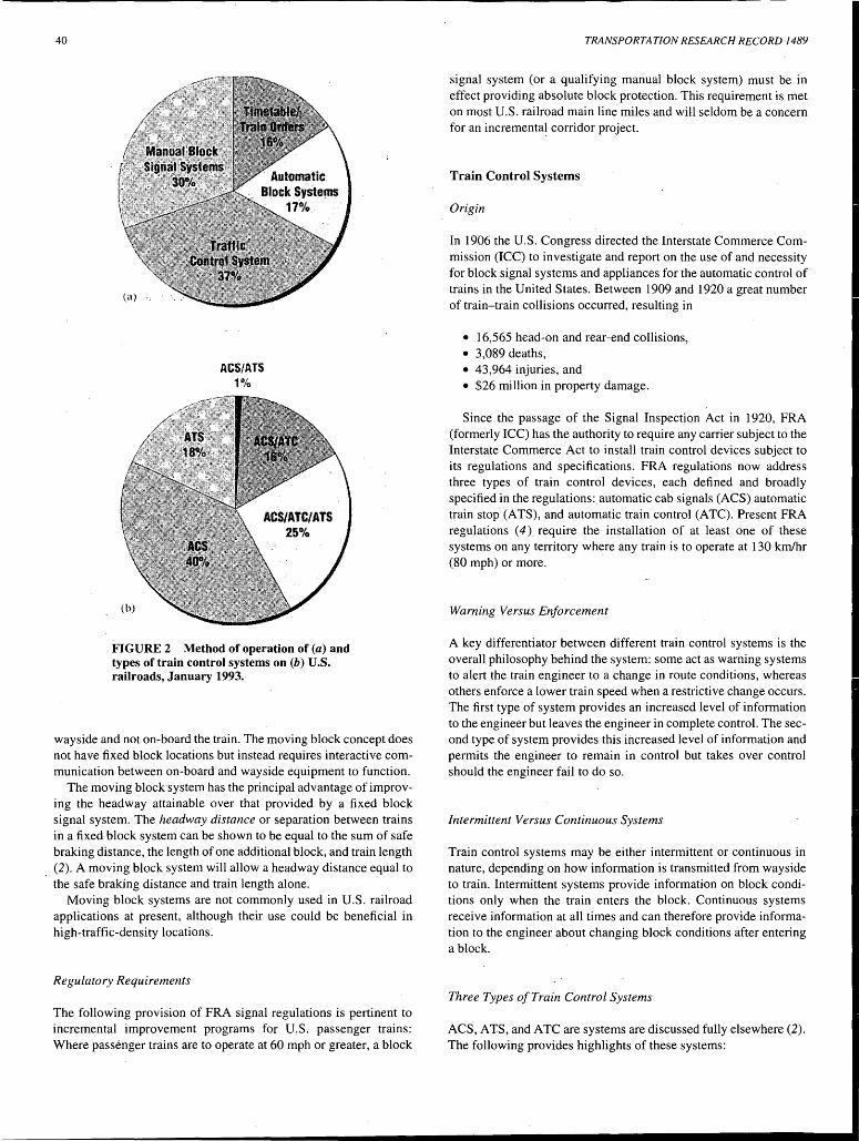
40

ACS/ATS 1%

FIGURE 2 Method of operation of (a) and types of train control systems on (b) U.S. railroads, January 1993.

wayside and not on-board the train. The moving block concept does not have fixed block locations but instead requires interactive com­munication between on-board and wayside equipment to function.

The moving blocksystem has the principal advantage of improv­ing the headway attainable over that provided by a fixed block signal system. The headway distance or separation between trains in a fixed block system can be shown to be equal to the sum of safe braking distance, the length of one additional block, and train length (2). A moving block system will allow a headway distance equal to the safe braking distance and train length alone.

Moving block systems are not commonly used in U.S. railroad applications at present, although their use could be beneficial in high-traffic-density locations.

Regulatory Requirements

The following provision of FRA signal regulations is pertinent to incremental improvement programs for U.S, passenger trains: Where passenger trains are to operate at 60 mph or greater, a block

TRANSPORTATION RESEARCH RECORD 1489

signal system (or a qualifying manual block system) must be in effect providing absolute block protection. This requirement is met on most U.S. railroad main line miles and will seldom be a concern for an incremental corridor project.

Train Control Systems

Origin

In 1906 the U.S. Congress directed the Interstate Commerce Com­mission (ICC) to investigate and report on the use of and necessity for block signal systems and appliances for the automatic control of trains in the United States. Between 1909 and 1920 a great number of train-train collisions occurred, resulting in

• 16,565 head-on and rear-end collisions, • 3,089 deaths, • 43,964 injuries, and • $26 million in property damage.

Since the passage of the Signal Inspection Act in 1920, FRA (formerly ICC) has the authority to require any carrier subject to the Interstate Commerce Act to install train control devices subject to its regulations and specifications. FRA regulations now address three types of train control devices, each defined and broadly specified in the regulations:_ automatic cab signals (ACS) automatic train stop. (A TS), and automatic train control (A TC). Present FRA regulations ( 4) require the installation of at least one of these systems on any territory wht:re any train is to operate at 130 km/hr (80 mph) or more.

Warning Versus Enforcement

A key differentiator between different train control systems is the overall philosophy behind the system: some act as warning systems to alert the train engineer to a change in route conditions, whereas others enforce a lower train speed when a restrictive change occurs. The first type of system provides an increased level of information to the engineer but leaves the engineer in complete control. The sec­ond type of system provides this increased level of information and permits the engineer to remain in control but takes over control should the engineer fail to do so.

Intermittent Versus Continuous Systems

Train control systems may be either intermittent or continuous in nature, depending on how information is transmitted from wayside to train. Intermittent systems provide information on block condi­tions only when the train enters the block. Continuous systems receive information at all times and can therefore provide informa­tion to the engineer about changing block conditions after entering a block.

Three Types of Train Control Systems

ACS, A TS, and A TC are systems are discussed fully elsewhere (2). The following provides highlights of these systems:

Ullman and Bing

• ACS Systems: ACS systems generally have from two to four aspects. If the train enters a restricted block the cab indicator dis­plays a restrictive indication and a whistle sounds. The engineer must depress an acknowledging lever or other device to silence the whistle, confirming his awareness of the condition. Note that the ACS system is open loop and does not interact with the train braking system. ·

• A TS Systems: ATS systems operate with the same wayside-to­train signals .(intermittent or continuous) as the ACS system, but A TS systems also have an interface with the train braking system. Entering a restricted block, a whistle sounds as for the ACS system and the engineer must again depress an acknowledging lever both to silence the audible indicator and to prevent an automatic application of the brakes. If the train receives a restrictive indication from the A TS system and the engineer does not take any action, a full-service brake application will occur after a delay not exceeding 8 sec.

• ATC (Speed Control) Systems: Full ATC systems are enforce­ment systems in that train speed is reduced directly by the system unless the train' s speed is similarly reduced under the control of the engineman. These systems operate with continuous coded track cir­cuits and also include an on-board speed generator. Train speed is continuously compared with the speed permitted by the relevant signal indication. Even operating under a·. nonrestrictive signal indication, the MAS for the train is enforced; that is, an overspeed condition will result in an audible indication and an automatic service brake application until the train speed is reduced to MAS (as determined by the setting of the on-board governor).

A TC speed enforcement ·applies to both passenger and freight vehicles equipped with A TC systems, and some freight lines oper­ate in this manner. Other freight carriers have petitioned for relief of the automatic full-service penalty applications from the A TC system, citing problems in train handling, particularly in undulating terrain. In response to these petitions FRA has permitted the re­moval of ATC systems from freight locomotives in some instances.

Present Application of Train Control Systems in the United States

Figure 2(b) summarizes the present application of train control systems in the United States as of January 1993 (3). A total of 15 750 track-km (9,843 track-mi), or 6.0 percent of the total U.S. rail network, is equipped with one or more train control systems.

ATC Systems

A number of systems of train control are being developed world­wide. These systems are based on advanced digital communications technology, but they are still in experimental stages and have not been approved for use as basic signal/train control systems in U.S. passenger corridors (2).

U.S. Incremental Corridor Track and Signal Configurations

Development of Hypothetical Corridors

The project described here analyzed hypothetical corridors repre­senting the Section 1010 corridors in the aggregate. From an exam-

41

ination of the corridors three typical cases seemed particularly appropriate for further analysis.

Case A: Single Track and Passing Sidings Many of the Section 1010 corridors have this structure, at least i.n part. Typical values evaluated were sidings of 2.4 km (1.5 mi) in length spaced every 32 km (20 mi), with operation under CTC rules. Hourly pas­senger trains [at a MAS of 145 km/hr (90 mph)] were projected to operate in each direction across the territory, in competition with light to moderate freight traffic of three daylight freight trains in each direction during the 14-hr daylight period. The freight trains were assumed to have MAS of 80 km/hr (50 mph).

Case B: Double-Track ABS System This fairly common arrangement consists of a full double track, with each track signaled for movements with the current of traffic. Interlockings are present every 24 km (15 mi), and these are configured so that trains may meet and pass at these points. Between interlockings, however, trains normally follow one another on the designated track. Passen­ger traffic was as for Case A, except at a MAS. of 175 km/hr (110 mph); base freight traffic was as for Case A.

Case C: Double-Track CTC This arrangement is not uncom­mon in highly used corridors, particularly if passenger service has always been a strong factor. Under the CTC scenario there is no current of traffic. Interlockings (simple universal crossovers) were assumed to be spaced every 16 km (10 mi); trains may pass on the links between interlockings. Passenger service is as outlined for Case A; however, MASs of 145, 175, 200, and 240 km/hr (90, 110, 125, and 150 mph) were considered. Base freight service was as for Case A.

Efficient Corridor Use

Corridor efficiency refers to the ability of a rail line to handle traf­fic smoothly, without undue delay. Efficiency depends on the way in which the rail line is constructed (infrastructure), the way in which it is used (operations), and the traffic requirements placed on it (demand). Dispatching controls railway operations; the present study assumed that it is done efficiently and equitably.

Headway and Capacity

Headway refers to the minimum interval, either in time or in dis­tance, between trains traveling in the same direction on a track. Safe braking distance assumes the worst-case location of trains in blocks, that is, closest together. Headway calculations must assume the opposite. This has the effect of adding an additional block length and the train length into the headway distance.

By using braking rates from the NEC example cited earlier, the addition of an additional block length, train length, and sight dis­tance to the 3447-m (11,300-ft) safe braking distance results in a headway distance of approximately 5490 m (18,000 ft). At 200 km/hr (125 mph) this means that 36 trains could pass a given point in a · 1-hr period; equivalently, a single track with unidirectional traffic has a theoretical capacity of 36 trains/hr and a theoretical

42

minimum headway of 99 sec with a perfectly uniform and opti­mized block layout. The use of more typical actual NEC block dis­tances (which accommodate freight operations as well) reduces this to a theoretical capacity of 28 trains/hr and 125-sec headways, but this still represents an idealized railroad.

Headway and capacity are reduced from the idealized theoreti­cal values by uneven block spacing and grade effects, trains of dif­ferent maximum speeds and lengths, civil speed restrictions (those not traffic or route dependent) present on the route, differences in train handling between enginemen, trains operating off schedule, and other random events. Capacity in the vicinity of even 20 trains/hr nevertheless provides for movement of a very large amount of traffic.

The presence of different train speeds greatly affects the practi­cal capacity of the line. In the example cited earlier, inserting a short express freight train operating at 95 km/hr (60 mph) into the traffic stream would reduce the throughput of the system from 28 trains/hr to 13 trains/hr, on a theoretical basis. If the freight train was 1525 m (5,000 ft) long rather than short, the capacity would drop to 11 trains/hr. The solution to these problems lies in scheduling slower freight trains out of passenger train hours or away from pas­senger trains where possible and in adding infrastructure to permit faster trains to overtake and pass slower trains.

Stringline Model

To demonstrate the impacts of freight train-passenger train interac­tion and to provide a tool for use during corridor development, a simplified, personal computer-based, manually dispatched rail operations model was developed and tested on the three hypotheti­cal corridofs. The simplified model is a link-and-node representa­tion of a raliway over which trains operate at assumed average speeds. The model output consists of stringline (time-distance) charts and delay statistics.

In the present study the average speed of the passenger train was taken as 80 percent of the stated MAS and the average speed of the freight train was taken as 70 percent of a 50-mph MAS, or 35 mph. The relatively low average speed chosen for freight trains is a con­servative assumption.

Passenger trains were assumed to operate hourly in each direc­tion across the approximately 500-km (310-mi) corridors. This level was chosen to illustrate peak service conditions on a typical corri­dor, but it may be insufficient if demand is heavy.

Three daylight freight trains scheduled in an irregular quasiran­dom manner were assumed to operate in each direction on the cor­ridor. All freight trains were assumed to be no longer than 1.5 mi.

Operating without interference, the freight trains would require 8 hr 49 min (8:49) to complete their run, and the passenger trains would require the following times: at a 90-mph MAS, 4:22; at a 110-mph MAS, 3:35; at a 125-mph MAS, 3:10; and at a 150-mph MAS, 2:39.

Train Interference-Case A: Single Track and Passing Sidings When all passenger trains (but no freights trains) are used in the simulation the resulting average passenger train delay was 21 min/train and ranged from 3 to 44 min. Such a large delay range is hard to handle. A schedule pad can be inserted to account for a rel­atively narrow band of delays, but a range this· wide indicates erratic performance at best. Under Case A conditions passenger train traf-

TRANSPORTATION RESEARCH RECORD 1489

fie alone produces significant interference, even with no freight train service being operated.

Figure 3 shows a stringline chart of the same passenger ti-afo traffic with only one freight train. The impacts are pronounced, as can be seen in Figure 3. Average passenger train delay increased by 85 percent, to 39 min, with a range of 3 to 143 min; five passenger trains were delayed in excess of 1 hr. The freight train was delayed 96 min. It is likely that different dispatching could improve the results for the train passenger at the expense of a delay for the freight train, but holding the freight train in one of the passing sidings means that a passing maneuver between opposing passenger trains now takes place over a 40-mi segment rather than a 20-mi segment, and. the transit time alone for such a link is 34 min. Other solutions are clearing the freight train off to an inter­mediate yard or switching siding, the use of more frequent sidirigs, the use of segments of double track to allow running meets, or expanding the complexity of the passing siding to allow for three~ train meets (additional tracks or crossovers to provide several pockets).

Train Interference-Case B: Double-Track ABS System Good train performance with all 28 passenger trains and 6 freight trains was achieved. The delay statistics are interesting:

Freight train delay Passenger train delay Total delay Freight train delay/train Passenger train delay/train Passenger train delay range Average delay/train

Minutes of Delay

90 mph 110 mph

463 177 640 77 6 6-15 19

491 145 636 82 5 3-16 19

Total train delay did not increase in going from the 90-mph case io the 110-mph case, showing the benefit of reduced transit time. Freight train delay has dropped from that in Case A, and passenger train delay is low and relatively uniform. Slight schedule adjust;.. ments to freight train departure times could reduce delays further. T~is is certainly an acceptable passenger train operation, and freight train performance may well be found to be acceptable in many instances. Freight train operations more intense than those tested are possible with this configuration.

Train Interference-Case C: Double-Track CTC System The same schedule of trains operated in Case B is operated in _Case C, with passenger train MASs of 90, 110, 125, and 150 mph, with the following results:

Minutes of Delay

90mph 110 mph 125 mph 150mph

Freight train delay 247 71 83 41 Passenger train delay 157 139 199 188 Total delay 404 210 282 229 Freight train delay/train 41 12 14 7 Freight train delay range 21-53 1-23 4-32 1-14 Passenger train delay/train 6 5 7 7 Passenger train delay range 5-17 3-17 6-13 5-17 Average delay/train 12 6 8 7

These results are much improved over those for Case B, with average total delay falling from 19 mins/train to as low as one-third

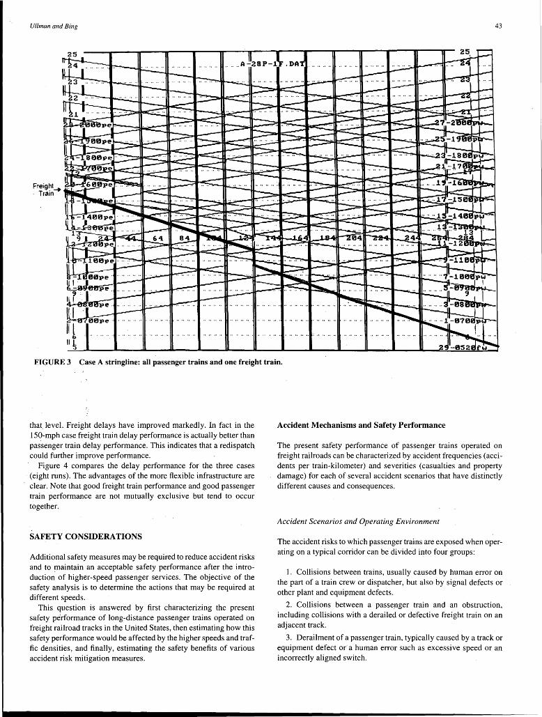
Ullman and Bing 43

FIGURE 3 Case A stringline: all passenger trains and one freight train.

that. level. Freight delays have improved markedly. In fact in the 150-mph case freight train delay performance is actually better than passenger train delay performance. This indicates that a redispatch could further improve performance.

Figure 4 compares the delay performance for the three cases (eight runs). The advantages of the more flexible infrastructure are clear. Note that good freight train performance and good passenger train performance are not mutually exclusive but tend to occur together.

SAFETY CONSIDERATIONS

Additional safety measures may be required to reduce accident risks and to !Uaintain an acceptable safety performance after the intro­duction of higher-speed passenger services. The objective of the safety analysis is to determine the actions that may be required at different speeds.

This question is answered by first characterizing the present safety performance of long-distance passenger trains operated on freight railroad tracks in the United States, then estimating how this safety performance would be affected by the higher speeds and traf­fic densities, and finally, estimating the safety benefits of various accident risk mitigation measures.

Accident Mechanisms and Safety Performance

The present safety performance of passenger trains operated on freight railroads can be characterized by accident frequencies (acci­dents per train-kilometer) and severities (casualties and property damage) for each of several accident scenarios that have distinctly different causes and consequences.

Accident Scenarios and Operating Environment

The accident risks to which passenger trains are exposed when oper­ating on a typical corridor can be divided into four groups:

1. Collisions between trains, usually caused by human error on the part of a train crew or dispatcher, but also by signal defects or other plant and equipment defects.

2. Collisions between a passe.nger train and an obstruction, including collisions with a derailed or defective freight train on an adjacent track.

3. Derailment of a passenger train, typically caused by a track or equipment defect or· a human error such as excessive speed or an incorrectly aligned switch.

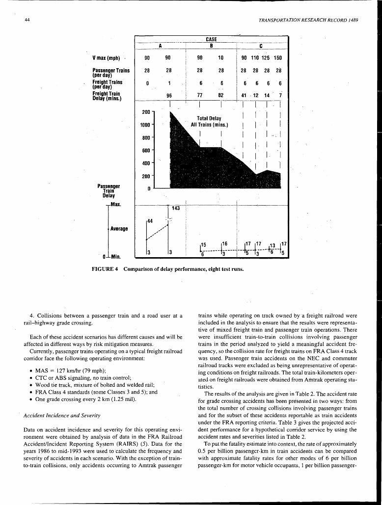
44 TRANSPORTATION RESEARCH RECORD 1489

CASE --·---·------··-··-----

A B c ---------·----;--------~----=------11

V max(mph) -

Passenger Trains (per day) Freight Trains (per day) Freight Train Delay (mlns.)

Passenger Train Delay

Max.

Average

0 Min.

90 90

28 28

0 i

96

200

1000

.800

600

. 400

200

0

143

90 10 90 110 125 150

28 28 28 28 28 28

6 6 6 6 6 ·5

77 82 41 12 14 7

I

Total Delay I All Trains (mins.) I

I I I I ·I·

I

FIGURE 4 Comparison of delay performance, eight test runs.

4. Collisions between a passenger train and a road user at a rail-highway grade crossing.

Each of these ;iccident scenarios has different causes and will be affected in different ways by risk mitigation measures.·

Currently, passenger trains operating on a typical freight railroad corridor face the following operating environment:

• MAS = 127 km/hr (79 mph); • CTC or ABS signaling, no train control; • Wood tie track, mixture of bolted and welded rail; • FRA Class 4 standards (some Classes 3 and 5); and • One grade crossing every 2 km (l.25 mil).

Accident Incidence and Severity

Data on accident incidence and severity for this operating envi­ronment were obtained by analysis of data in the FRA Railroad Accident/Incident Reporting System (RAIRS) (5). Data for the years 1986 to mid-1993 were used to ·calculate the frequency and severity of accidents in each scenario. With the exception of train­to-train collisions, only accidents occurring to Amtrak passenger

trains while operating on track owned by a freight railroad were included in the analysis to ensure that the results were representa­tive of mixed freight train and passenger train operations. There were insufficient train-to-train collisions involving passenger trains in the period analyzed to yield a meaningful accident fre­quency, so the collision rate for freight trains on FRA Class 4 track was used. Passenger train accidents on the NEC and commuter railroad tracks were excluded as being unrepresentative of operat­ing conditions on freight railroads. The total train-kilometers oper­ated on freight railroads were obtained from Amtrak operating sta­tistics.

The results.of the analysis are given in Table 2. The accident rate for grade crossing accidents has been presented in two ways: from the total number of crossing collisions involving passenger trains and for the subset of these accidents reportable as train accidents under the FRA reporting criteria. Table 3 gives the projected acci­dent performance for a hypothetical corridor service by using the accident rates and severities listed in Table 2.

To put the fatality estimate into context, the rate of approximately 0.5 per billion passenger-km in train accidents can be compared with approximate fatality rates for other modes of 6 per billion passenger-km for motor vehicle occupants, 1 per billion passenger-

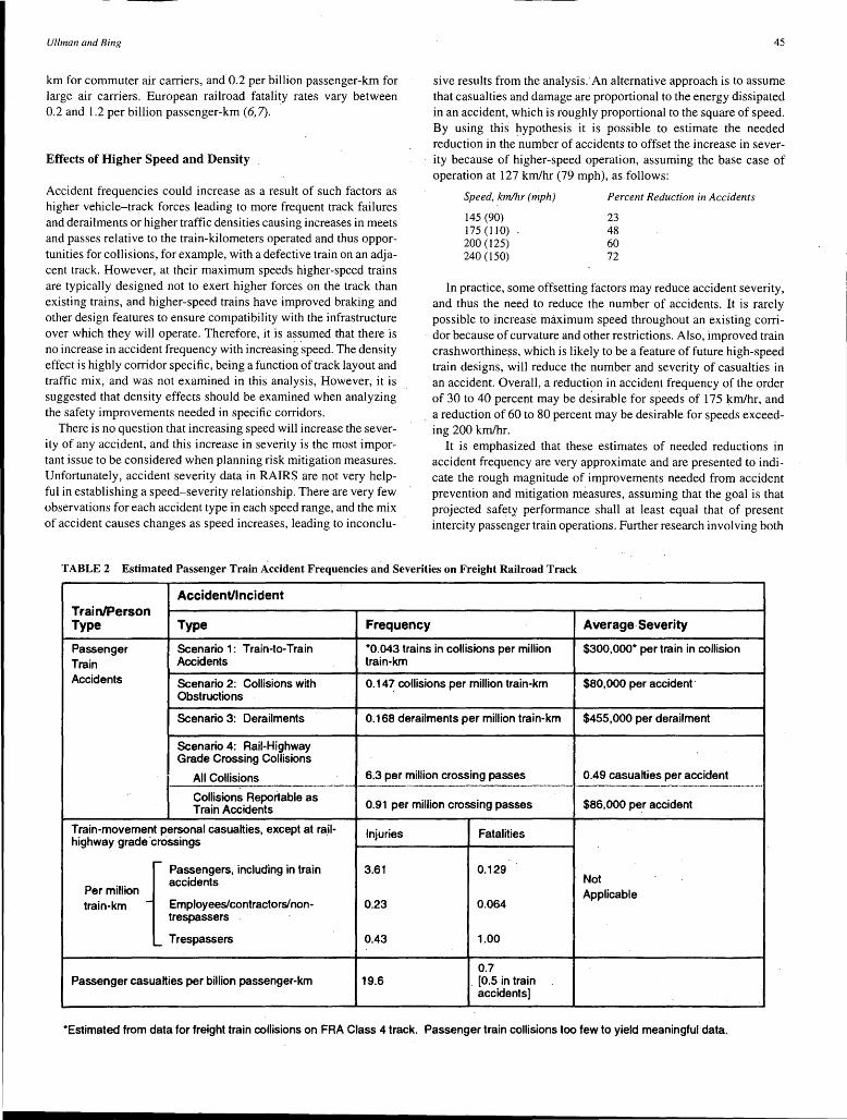
Ullman and Bing

km for commuter air carriers, and 0.2 per billion passenger-km for large air carriers. European railroad fatality rates vary between 0.2 and 1.2 per billion passenger-km ( 6, 7).

Effects of Higher Speed and Density

Accident frequencies could increase as a result of such factors as higher vehicle-track forces leading to more frequent track failures and derailments or higher traffic densities causing increases in meets and passes relative to the train-kilometers operated and thus oppor­tunities for collisions, for example, with a defective train on an adja­cent track. However, at their maximum speeds higher-speed trains are typically designed not to exert higher forces on the track than existing trains, and higher-speed trains have improved braking and other design features to ensure compatibility with the infrastructure over which they will operate. Therefore, it is assumed that there is no increase in accident frequency with increasing speed. The density effect is highly corridor specific, being a function of track layout and traffic mix, and was not examined in this analysis, However, it is suggested that density effects should be examined when analyzing the safety improvements needed in specific corridors.

There is no question that increasing speed will increase the sever­ity of any accident, and this increase in severity is the most impor­tant issue to be considered when planning risk mitigation measures. Unfortunately, accident severity data in RAIRS are not very help­ful in establishing a speed-severity relationship. There are very few observations for each accident type in each speed range, and the mix of accident causes changes as speed increases, leading to inconclu-

45

sive results from the analysis.· An alternative approach is to assume that casualties and damage are proportional to the energy dissipated in an accident, which is roughly proportional to the square of speed. By using this hypothesis it is possible to estimate the needed reduction in the number of accidents to offset the increase in sever­ity because of higher-speed operation, assuming the base case of operation at 127 km/hr (79 mph), as follows:

Speed, km/hr (mph)

145 (90) 175(110) 200 (125) 240 (150)

Percent Reduction in Accidents

23 48 60 72

In practice, some offsetting factors may reduce accident severity, and thus the need to reduce the number of accidents. It is rarely possible to increase maximum speed throughout an existing corri­dor because of curvature and other restrictions. Also, improved train crashworthiness, which is likely to be a feature of future high-speed train designs, will reduce the number and severity of casualties in an accident. Overall, a reduction in accident frequency of the order of 30 to 40 percent may be de.sirable for speeds of 175 km/hr, and a reduction of 60 to 80 percent may be desirable for speeds exceed­ing 200 km/hr.

It is emphasized that these estimates of needed reductions in accident frequency are very approximate and are presented to indi­cate the rough magnitude of improvements needed from accident prevention and mitigation measures, assuming that the goal is that projected saf~ty performance shall at least equal that of present intercity passenger train operations. Further research involving both

TABLE 2 Estimated Passenger Train Accident Frequencies and Severities on Freight Railroad Track

Accident/Incident Train/Person Type Type Frequency Average Severity

Passenger Scenario 1: Train-to-Train *0.043 trains in collisions per million $300,000* per train in collision Train Accidents train-km

Accidents Scenario 2: Collisions with 0.14~ collisions per million train-km $80,000 per accident· Obstructions

Scenario 3: Derailments 0.168 derailments per million train-km $455,000 per derailment ·

Scenario 4: Rail-Highway Grade Crossing Collisions

All Collisions 6.3 per million crossing passes 0.49 casualties per accident ... _. ___ -·--·- --- ----------·------·-....----Collisions Reportable as

0.91 per million crossing passes $86,000 per accident Train Accidents

Train-movement personal casualties, except at ra.il- Injuries Fatalities highway grade 'crossings

{ Passengers, including in train 3.61 0.129 accidents Not

Per million Applicable train-km Employees/contractors/non- 0.23 0.064

trespassers . · ·

Trespassers 0.43 1.00

0.7 Passenger casualties per billion passenger-km 19.6 . [0.5 in train

accidents]

*Estimated from data for freight train collisions on FRA Class 4 track. Passenger train collisions too few to yield meaningful data.

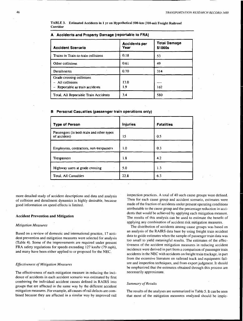
46 TRANSPORTATION RESEARCH RECORD 1489

TABLE 3. Estimated Accidents in 1 yr on Hypothetical 500-km (310-mi) Freight Railroad Corridor

A Accidents and Property Damage (reportable to FRA)

Accidents per Total Damage Accident Scenario Vear $1000s

Trains in Train-to-train co11isions 0.18 53

Other collision.~ 0.61 49

Derailments 0.70 314

Grade crossing collisions - All collisions 13.0 ----- Reportable as train accidents 1.9 162

Total, All Reportable Train Accidents 3.4 580

B Personal Casualties (passenger train operations only)

Type of Person

Passengers (in both train and other types of accident)

Employees, contractors, non-trespassers

Trespassers

Highway users at grade crossing

Total, All Casualties

more detailed study of accident descriptions and data and analysis of collision and derailment dynamics is highly desirable, because good information on speed effects is limited.

Accident Prevention and Mitigation

Mitigation Measures

Based on a review of domestic and international practice, 17 acci­dent prevention and mitigation measures were selected for analysis (Table 4). Some of the improvements are required under present FRA safety regulations for speeds exceeding 127 km/hr (79 mph), and many have been either applied to or proposed for the NEC.

Effectiveness of Mitigation Measures

The effectiveness of each mitigation measure in reducing the inci­dence of accidents in each accident scenario was estimated by first combining the individual accident causes defined in RAIRS into groups that are affected in the same way by the different accident mitigation measures. For example, all causes of rail defects are com­bined because they are affected in a similar way by improved rail

Injuries Fatalities

15 0.5

1.0 0.3

1.8 4.2

5.0 1.3

22.8 6.3

inspection practices. A total of 40 such cause groups were defined. Then for each cause group and accident scenario, estimates were made of the fraction of accidents under present operating conditions attributable to the cause group and the percentage reduction in acci­dents that would be achieved by applying each mitigation measure. The results of this analysis can be used to estimate the benefit of applying any combination of accident risk mitigation measures.

The distribution of accidents among cause groups was based on an analysis of the RAIRS data base by using freight train accident data to guide estimates when the sample of passenger train data was too small to yield meaningful results. The estimates of the effec­tiveness of the accident mitigation measures in reducing accident incidence were derived in part from a comparison of passenger train accidents in the NEC with accidents on freight train trackage, in part from the extensive literature on railroad track and equipment fail­ure and inspection techniques, and from expert judgment. It should be emphasized that the estimates obtained through this process are necessarily approximate.

Summary of Results

The results of the analyses are summarized in Table 5. It can be seen that most of the mitigation measures analyzed should be imple-

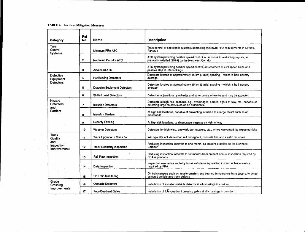
TABLE 4 Accident Mitigation Measures

Ref Category No. Name Description

Train Train control or cab signal system just meeting minimum FRA requirements in CFR49, Control 1 Minimum FRA ATC Part 236 Systems

2 Northeast Corridor A TC ATC system providing positive speed control in response to restricting signals, as presently installed (1994) on the Northeast Corridor

Advanced ATC ATC system providing positive speed control; enforcement of civil speed limits and

3 positive stop at interlockings

Defective Detectors located at approximately 15 km (9 mile) spacing -- which is half industry Equipment 4 Hot Bearing Detectors average

Detectors Detectors located at approximately 15 km (9 mile) spacing -- which is half industry

5 Dragging Equipment Detectors average

6 Shifted Load Detectors Detectors at junctions, yard exits and other points where hazard may be expected

Hazard Detectors at high-risk locations, e.g., overbridges, parallel rights-of-way, etc., capable of Detectors 7 Intrusion Detectors detecting large objects such as an automobile and Barriers At high risk locations, capable of preventing intrusion of a large object such as an

8 Intrusion Barriers automobile

9 Security Fencing At high risk locations, to discourage trespass on right of way

10 Weather Detectors Detectors for high wind, snowfall, earthquakes, etc., where warranted by expected risks

Track Track Upgrade to Class 6+ Will typically include welded rail throughout, concrete ties and elastic fasteners Quality 11

and Reducing inspection intervals to one month. as present practice on the Northeast Inspection 12 . Track Geometry Inspection Corridor Improvements

. Rail Flaw Inspection Reducing inspection intervals to six months from present annual inspection required by

13 FRA reoulations

Inspection over entire route by hi-rail vehicle or equivalent, instead of twice weekly 14 Daily Inspection required by FRA

On Train Monitoring On train sensors such as acce.lerometers and bearing temperature transducers, to detect

.15 selected vehicle and track defects

Grade Obstacle Detectors Crossing 16 Installation of a stalled-vehicle detector at all crossinos in corridor

Improvements Four.Quadrant Gates Installation of fo~r-quadrant crossing gates at all crossings in corridor 17

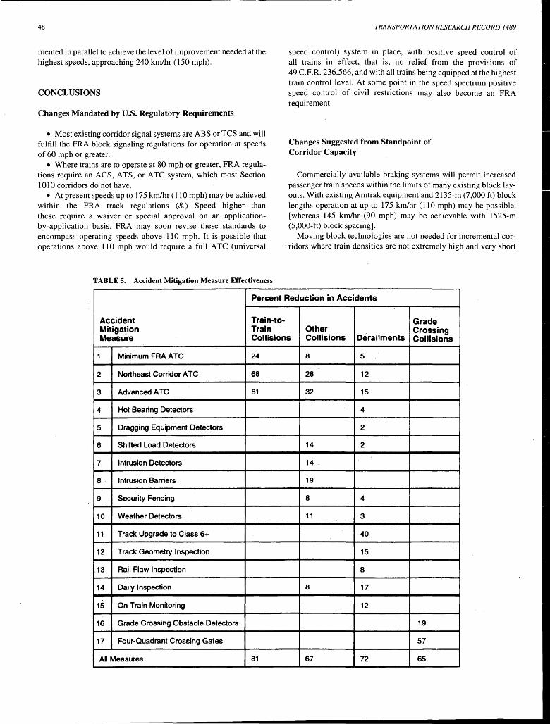
48

mented in parallel to achieve the level of improvement needed at the highest speeds, approaching 240 km/hr (150 mph).

CONCLUSIONS

Changes Mandated by U.S. Regulatory Requirements

• Most existing corridor signal systems are ABS or TCS and will fulfill the FRA block signaling regulations for operation at speeds of 60 mph or greater.

• Where trains are to operate at 80 mph or greater, FRA regula­tions require an ACS, ATS, or A TC system, which most Section 1010 corridors do not have.

• At present speeds up to 17 5 km/hr ( 110 mph) may be achieved within the FRA track regulations (8.) Speed higher than these require a waiver or special approval on an application­by-application basis. FRA may soon revise these standards to encompass operating speeds above 110 mph. It is possible that operations above 110 mph would require a full ATC (universal

TABLE 5. _Accident Mitigation Measure Effectiveness

TRANSPORTATION RESEARCH RECORD 1489

speed control) system in place, with positive speed control of all trains in effect, that is, no relief from the provisions of 49 C.F.R. 236.566, and with all trains being equipped at the highest train control level. At some point in the speed spectrum positive speed control of civil restrictions may also become an FRA requirement.

Changes Suggested from Standpoint of Corridor Capacity

Commercially available brakjng systems will permit increased passenger train speeds within the limits of many existing block lay­outs. With existing Amtrak equipment and 2135-m (7,000 ft) block lengths operation at up to 175 km/hr (110 mph) may be possible, [whereas 145 km/hr (90 mph) may be achievable with 1525-m (5,000-ft) block spacing].

Moving block technologies are not needed for incremental cor­. ridors where train densities are not extremely high and very short

Percent Reduction in Accidents

Accident Train-to- Grade Mitiga~ion Train Other Crossing Measure Collisions Collisions Derailments Collisions

1 Minimum FAA ATC 24 8 5

2 Northeast Corridor A TC 68 28 12

3 Advanced A TC 81 32 15

4 Hot Bearing Detectors 4

5 Dragging Equipment Detectors 2

6 Shifted Load Detectors 14 2

7 Intrusion Detectors 14

8 Intrusion Barriers 19

9 Security Fencing 8 4

10 Weather Detectors 11 3

11 Track Upgrade to Class 6+ 40

12 Track Geometry Inspection 15

.13 Rail Flaw Inspection 8

14 Daily Inspection 8 17

15 On Train Monitoring 12

16 Grade Crossing Obstacle Detectors 19

17 Four-Quadrant Crossing Gates 57

All Measures 81 67 72 65

Ullman and Bing

headways are not required. Currently available A TC systems are not yet capable enough for stand-alone use in incremental corri­dors.

Single-track corridors will face difficulties if passenger train and significant freight train operations must both operate during the same time periods. Although some service is obviously possible, there are limits to what can be achieved with such an infrastructure. There is also the potential for significant schedule unreliability, which could adversely affect the marketability of the service provided.

Detailed, site-specific studies must be performed to match the traffic requirements and the infrastructure proposed, with accept­able delays to freight and passenger train services as a constraint.

Additional· parallel running tracks, increased siding lengths, decreased siding spacings, more complex interlockings, and re­verse running capability are key infrastructure components to be considered.

Adjusting passenger and freight train schedules and establishing priority passenger (freight blackout) periods are key operating con­siderations to be considered.

Changes Suggested from Standpoint of Safety

The overall conclusion from the present study is that a large num­ber of accident risk mitigation measures may need to be imple­mented in parallel if present intercity rail safety performance is to be maintained with higher-speed operation on a freight railroad cor­ridor.· Key measures that deserve consideration, some of which would be required under present FRA regulations, are

• An A TC system having functional performance similar to that used or proposed in the NEC.

49

• Track improvement to FRA Class 6 or better, with enhanced inspection.

• Improved rail-highway grade crossing warning systems, new protection systems, and/crossing elimination where practical.

• Improved defect and hazard warning systems.

ACKNOWLEDGMENTS

The authors gratefully acknowledge the financial support and encouragement provided by the Volpe National Transportation Systems Center and FRA, which are sponsors of this study.

REFERENCES

1. Pub. L. 102-240 (Dec. 18, 1991), Intermodal Surface Transportation Efficiency Act of 1991 (ISTEA). 105 stat. 1914.

2. Ullman, K. B., and A. J. Bing. High Speed Passenger Trains in Freight Railroad Corridors: Operations and Safety Considerations. Report DOT­VNTSC-FRA-94-11. U.S. Department of Transportation, Nov. 1994.

3. Annual Report-Method of Train Operation as of January 1, 1993. FRA, U.S. Department of Transportation.

4. Rules, Standards, and Instructions Governing the Installation, Inspec­tion, Maintenance, and Repair of Signal and Train Control Systems, Devices, and Appliances. 49 C.F.R. 236.

5. Railroad Accident/Incident Reporting System (RA/RS) Database of Railroad Accidents, Incidents, and Grade Crossing Accidents, Jan. 1986-June 1993 inclusive. FRA, U.S. Department of Transportation.

6. National Safety Council. Accident Facts, 1992. 7. Bing, A. J., J. A. Harrison, et al. Safety of HSGGT Systems: Collision

Avoidance and Accident Survivability. Report DOT-FRA-ORD-93/04 (four volumes). FRA, U.S. Department of Transportation, March 1993.

8. Federal Track Safety Standards. 49 C.F.R. 213.57 et seq.

Publication of this paper sponsored by Committee on Guided Intercity Passenger Transportation.

50 TRANSPORTATION RESEARCH RECORD 1489

Evaluation of Selected Crashworthiness Strategies for Passenger Trains

D. TYRELL, K. SEVERSON~GREEN, AND B. MARQUIS

Interest in high-speed passenger rail has increased recently. The poten­tial for collisions at increased speeds has renewed concerns about the crashworthiness of passenger rail vehicles. Studies have been con­ducted to evaluate the effectiveness of alternative strategies for provid­ing for the crashworthiness of the vehicle ·Structures and interiors at increased collision speeds. Conventional practice has resulted in cars of essentially uniform longitudinal strength. This approach has been found to be effective for train-to-train collision speeds of up to 31 m/sec (70 mph). This uniform strength causes the structural crushing of the train to proceed uniformly through both the unoccupied and occupied areas of the train. The crash energy management approach results in varying longitudinal strength, with high strength in the occupied areas and lower strength in the unoccupied areas. This approach attempts to distribute the structural crushing throughout the train to the unoccupied areas to preserve the occupant volumes and to limit the decelerations of the cars. The crash energy management approach has been found to offer significant benefits for higher-speed collisions. The interior crash­worthiness analysis evaluated the influence of interior configuration and occupant restraint on fatalities resulting from occupant motions during a collision. For a sufficiently gentle train deceleration, compartmental­ization (a strategy for providing a "friendly" interior) can provide suf­ficient occupant protection to keep accepted injury criteria below the threshold values applied by the automotive industry. The use of seat belts and shoulder restraints reduces the likelihood of fatalities due to deceleration to near-certain survival for even the most severe collision conditions considered.

Interest in high-speed passenger rail, with speeds in excess of 56 m/sec (125 mph), has increased recently. The potential for collisions at increased speeds and collisions involving passenger vehicles and vehicles with substantially different structures has renewed concerns about the crashworthiness of passenger rail vehi­cles. Studies have been conducted to evaluate the effectiveness of alternative strategies for providing for the crashworthiness of the vehicle structures and interiors at increased collision speeds. This paper describes comparisons of strategies for ensuring the structural crashworthiness of passenger vehicles and describes comparisons of strategies for ensuring interior crashworthiness for the protection of occupants of the train during collisions.

BACKGROUND

Trains may collide with objects that are relatively small, such as an animal on the tracks, highway vehicles, maintenance-of-way equipment, or another train. Most of these collisions can only occur in the normal running direction of the train; however, impacts into

Structures and Dynamics Division, Office of Systems Engineering, Volpe National Transportation Systems Center, Research and Special Programs Administration, U.S. Department of Transportation, Kendall Square, Cambridge, Mass. 02142.

the side of the train can occur at grade crossings. Derailment can lead to the train rolling over, inducing high loads .into the sides of the cars and roof. Longitudinal collisions can occur at any speed up to the operating speed of the train. Highway vehicle collisions into the side of the train can occur at lower speeds.

In addition to the primary collision between the train and the impacted object, there is also a secondary collision between· the occupants and the interior. Causes of fatalities associated with' the primary collision include crushing of the occupant compartment, in which the occupants themselves are crushed, local penetration into the occupant compartment, in which an object intrudes into the occupant compartment and directly strikes an occupant, and occu­pant ejection from the occupant compartment, in which an occupant is thrown from the train and strikes some element on the wayside. Causes of fatalities associated with secondary collisions include excessive deceleration of the head or chest of the occupant and excessive forces imparted to the body, such as axial neck loads ..

In designing for crashworthiness the first objective is to preserve a minimum occupant volume for the occupants to ride out the collision. Preserving the occupant volume. is accomplished with structural strength; that is, if the occupant compartment is suffi­ciently strong, then there will be sufficient space.for the occupants to ride out the collision. The second objective is to limit the forces and decelerations imparted to the occupants to acceptable levels of human tolerance. Limiting the decelerations and forces is accom­plished through a combination of structural crashworthiness measures: allowing portions of the vehicle to be crushed in a pre­detep,nined manner, thereby limiting the decelerations of the vehi­cle; using interior crashworthiness measures, including occupant restraints, such as seat belts and shoulder harnesses; and applying strategies such as compartmentalization.

To evaluate the performance of a train in a particular collision, the collision mechanics of the train must be estimated or deter­mined, the likelihood of car-to-car override and lateral buckling of the train needs to be known, and the forces acting between cars and the crushing behavior of the cars must be developed. Once the behavior of the train has been determined, the interior performance can be evaluated. A detailed review of transportation crash worthi­ness practice and research and its applicability to passenger rail transportation is presented elsewhere (J).

STRUCTURAL CRASHWORTHINESS

Convi;,ntional practice has resulted in cars of uniform longitudinal strength. The crash energy management approach results in varying longitudinal strength throughout the train, with high strength in the occupied areas and lower strength in the unoccupied areas. This approach attempts to distribute the structural crushing through-

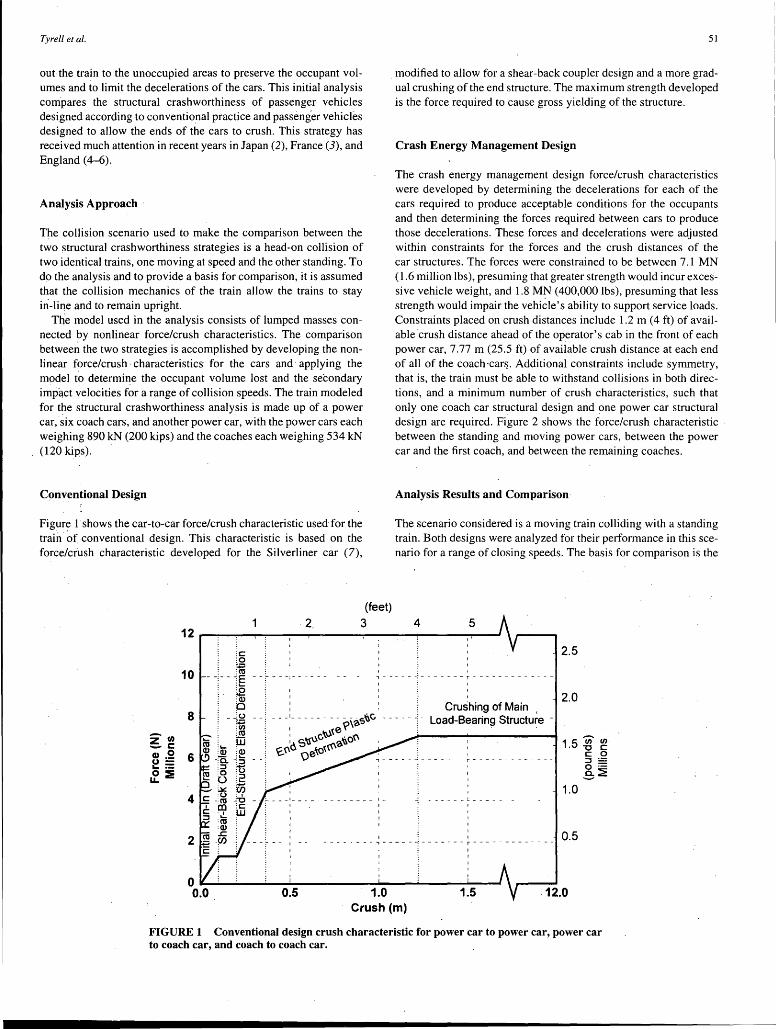
Tyrell et al.

out the train to the unoccupied areas to preserve the occupant vol­umes and to limit the decelerations of the cars. This initial analysis compares the structural crashworthiness of passenger vehicles designed according to conventional practice and passenger vehicles designed to allow the ends of the cars to crush. This strategy has received much attention in recent years in Japan (2), France (3), and England ( 4-6).

Analysis Approach

The collision scenario used to make the comparison between the two structural crashworthiness strategies is a head-on collision of two identical trains, one moving at speed and the other standing. To do the analysis and to provide a basis for comparison, it is assumed that the collision mechanics of the train allow the trains to stay in-line and to remain upright.

The model used in the analysis consists of lumped masses con­nected by nonlinear force/crush characteristics. The comparison between the two strategies is accomplished by developing the non­linear force/crush ·characteristics for the cars and· applying the model to determine the occupant volume lost and the secondary imp~ct velocities for a range of collision speeds. The train modeled for the structural crashworthiness analysis is made up of a power car, six coach cars, and another power car, with the power cars each weighing 890 kN (200 kips) and the coaches each weighing 534 kN (120 kips).

Cpnventional Design

Figur~ i -shows the car-to-car force/crush characteristic used for the train. of conventional design. This characteristic is based on the force/crush characteristic developed for the Silverliner car (7),

2. (feet)

3

51

modified to allow for a shear-back coupler design and a more grad­ual crushing of the end structure. The maximum strength developed is the force required to cause gross yielding of the structure.

Crash Energy Management Design

The crash energy management design force/crush characteristics were developed by determining the decelerations for each of the cars required to produce acceptable conditions for the occupants and then determining the forces required between cars to produce those decelerations. These forces and decelerations were adjusted within constraints for the forces and the crush distances of the car structures. The forces were constrained to be between 7. I MN (1.6 million lbs), presuming that greater strength would incur exces­sive vehicle weight, and 1.8 MN (400,000 lbs), presuming that less strength would impair the vehicle's ability to support service loads. Constraints placed on crush distances include 1.2 m (4 ft) of avail­able crush distance ahead of the operator's cab in the front of each power car, 7.77 m (25.5 ft) of available crush distance at each end of all of the coach ·cars. Additional constraints include symmetry, that is, the train must be able to withstand collisions in both direc­tions, and a minimum number of crush characteristics, such that only one coach car structural design and one power car structural design are required. Figure 2 shows the force/crush characteristic between the standing and moving power cars, between the power car and the first coach, and between the remaining coaches.

Analysis Results and Comparison

The scenario considered is a moving train colliding with a standing train. Both designs were analyzed for their performance in this sce­nario for a range of closing speeds. The basis for comparison is the

4 5 12 -----.---.-----.---.---.--~---.---.---.---.---.---.-----.---.---.---.--

10

8

z0 - c CD .2 6 "= .. ·-~ :E

4

2

~c

. ~ - -~- - -~

0 _ _:o

~ :m jii

I

., - - - - -I

I

- - - '- - - - - - - - - - -S~C - - - - -I e ~\'O : ~uc~~ ~o'(\

~'(\6~e\O~~~

--------I_ I

2.5

Crushing of Main . Load-Bearing Structure -

2.0

1.0 ______ !. _____ -

I

-- - - ~ - - - - - - - - - - - - ~ - - - - - - - - - - - - - 0.5

0 ._ __________ ....... ____ ___, ____ __. ______ ___, __ ___, ....... __ _,

0.0 0.5 1.0 Crush (m)

1.5 12.0

FIGURE 1 Conventional design crush characteristic for power car to power car, power car to coach car, and coach to coach car.

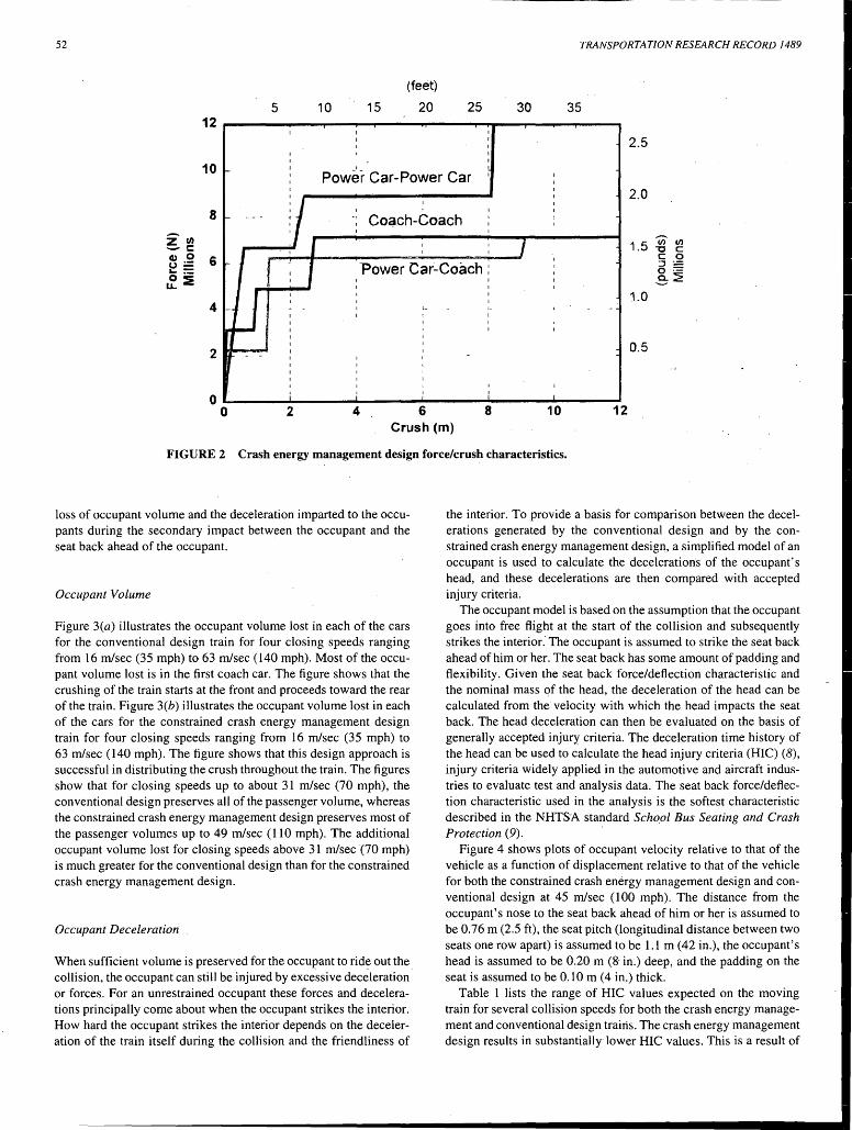
52

5 10 15 12

I I I

I I I I

(feet)

20 25

I I I I I I

TRANSPORTATION RESEARCH RECORD 1489

30 35

2.5

..... I Power Car-Power Car I I I I

10 I I I I 2.0 I I I I I I I I - - - - + -•. Coach-Coach ' I I I

8 I I , I I I I I I

I

1.5 ~ en "C c c 0 , ..... - Power Car-_Coach : I

I

j I

6 ::s 0 := .e 2 I I I I

I I I I

I I I

I I I

- I ,_ ·-4

1.0 I I I I

I I I - I I I

I I

I I

I I -I I I 2 0.5 I I I

I I I

I I I

I I I I I

0 : : : : I

0 2 4 6 Crush (m)

8 10 12

FIGURE 2 Crash energy management design force/crush characteristics.

loss of occupant volume and the deceleration imparted to the occu­pants during the secondary impact between the occupant and the seat back ahead of the occupant.

Occupant Volume

Figure 3(a) illustrates the occupant volume lost in each of the cars for the conventional design train for four closing speeds ranging from 16 m/sec (35 mph) to 63 m/sec (140 mph). Most of the occu­pant volume lost is in the first coach car. The figure shows that the crushing of the train starts at the front and proceeds toward the rear of the train. Figure 3(b) illustrates the occupant volume lost in each of the cars for the constrained crash energy management design train for four closing speeds ranging from 16 m/sec (35 mph) to 63 m/sec (140 mph). The figure shows that this design approach is successful in distributing the crush throughout the train. The figures show that for closing speeds up to about 31 m/sec (70 mph), the conventional design preserves all of the passenger volume, whereas the constrained crash energy management design preserves most of the passenger volumes up to 49 m/sec (110 mph). The additional occupant volume lost for closing speeds above 31 m/sec {70 mph) is much greater for the conventional design than for the constrained crash energy management design.

Occupant Deceleration

When sufficient volume is preserved for the occupant to ride out the collision, the occupant can still be injured by excessive deceleration or forces. For an unrestrained occupant these forces and decelera­tions principally come about when the occupant strikes the interior. How hard the occupant strikes the interior depends on the deceler­ation of the train itself during the collision and the friendliness of

the interior. To provide a basis for comparison between the decel­erations generated by the conventional design and by the con­strained crash energy management design, a simplified model of an occupant is used to calculate the decelerations of the occupant's head, and these decelerations are then compared with accepted injury criteria.

The occupant model is based on the assumption that the occupant goes into free flight at the start of the collision and subsequently strikes the interior. The occupant is assumed to strike the seat back ahead of him or her. The seat back has some amount of padding and flexibility. Given the seat back force/deflection characteristic and the nominal mass of the head, the deceleration of the head can be calculated from the velocity with which the head impacts the seat back. The head deceleration can then be evaluated on the basis of generally accepted injury criteria. The deceleration time history of the head can be used to calculate the head injury criteria (HIC) (8), injury criteria widely applied in the automotive and aircraft indus­tries to evaluate test and analysis data. The seat back force/deflec­tion characteristic used in the analysis is the softest characteristic described in the NHTSA standard Scho.ol Bus Seating and Crash Protection (9).

Figure 4 shows plots of occupant velocity relative to that of the vehicle as a function of displacement relative to that of the vehicle for both the constrained crash energy management design and con­ventional design at 45 m/sec (100 mph). The distance from the occupant's nose to the seat back ahead of him or her is assumed to be 0.76 m (2.5 ft), the seat pitch (longitudinal distance between two seats one row apart) is assumed to be 1.1 m (42 in.), the occupant's head is assumed to be 0.20 m (8- in.) deep, and the padding on the seat is assumed to be 0.10 m (4 in.) thick.

Table 1 lists the range of HIC values expected on the moving train for several collision speeds for both the crash energy manage­ment and conventional design trains. The crash energy management design results in substantially lower HIC values. This is a result of

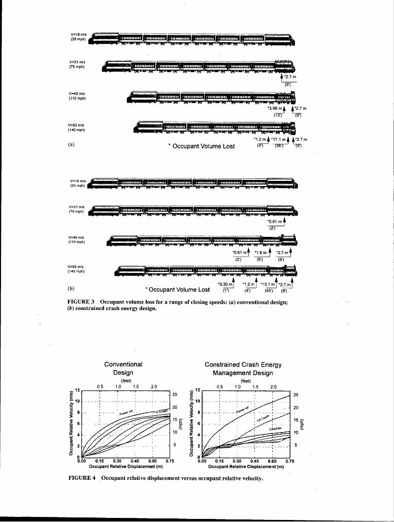
V=16m/s ,. -···· -(35 mph) J-- __ .

V=31 mis (70 mph)

V=49 mis (110 mph)

V=63 mis (140 mph)

(a)

,. · + *2.7m

(9')

*3.~ ~m

*Occupant Volume Lost ·1~·~~m

~~3

~;:~ •41iiiiill~1e~2~:~::,••~e!2~:!::,!•~e~2~:~::~. g••~e~2~:~::~1ee~2~:~::~•1ee~2!:~::~-i: :-:-·:· :i:t.'

V=49 mis (110mph)

V=63 mis (140 mph)

(b)

*0.61 m + (2')

,:- ---.:~-l22::2!eu2:::!tr22!::!&:2:::1:2:::trtt:a1tJl *0.61 mt ~ *2.7mt

(2') (6') (9')

,_. :ie2:::1zrnm::!&ut::::te2:::1J22~::t::m:31f: -=~~ *0.30 mt ·1~ •13d *2~

*Occupant Volume Lost (1') (4') (43') (9')

FIGURE 3 Occupant volume loss for a range of closing speeds: (a) conventional design; (b) constrained crash energy design.

0.5

0.15

Conventional Design

(feet) 1.0 1.5 2.0

0.30 0.45 0.60 Occupant Relative Displacement (m)

15 :2 a.. .s

10

5

0.75

Constrained Crash Energy Management Design

(feet)

~ 12 .--~~o-~5~---.1._o~--.1.5~~2~.o~----. ~ 25 ;10 ----­u .2 8 _____ :~--~ QI

~ 6 111 ii ir: 4 -... c 111 g. 2 u

~ 0.15 0.30 0.45 0.60

Occupant Relative Displacement (m)

20

5

0.75

FIGURE 4 _Occupant relative displacement versus occupant relative velocity.

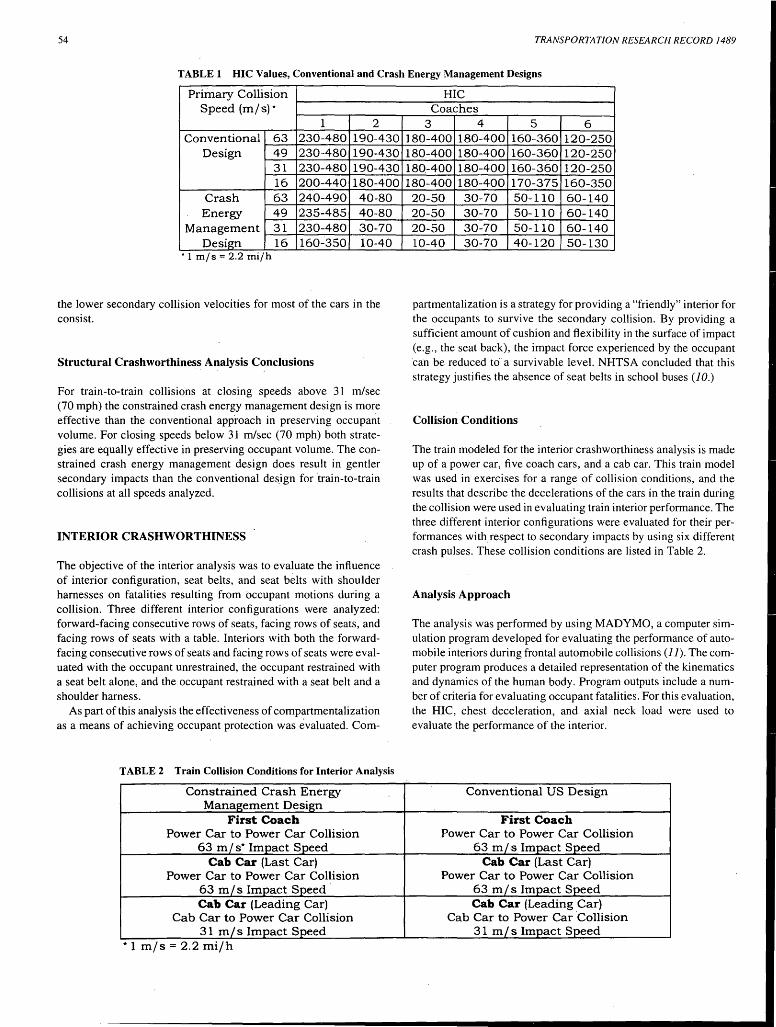
54 TRANSPORTATION RESEARCH RECORD 1489

TABLE 1 HIC Values, Conventional and Crash Energy Management Designs

Primary Collision Speed (m/s) •

HIC Coaches

1 2 3 4 5 6 Conventional 63 230-480 190-430 180-400 180-400 160-360 120-250

Design 49 230-480 190-430 180-400 180-400 160-360 120-250 31 230-480 190-430 180.-400 180-400 160-360 120-250 16 200-440 180-400 180-400 180-400 170-375 160-350

Crash 63 240-490 40-80 20-50 30-70 50-110 60-140 Energy 49 235-485 40-80

Management 31 230-480 30-70 Design 16 160-350 10-40

• 1 mis= 2.2 milh

the lower secondary collision velocities for most of the cars in the consist.

Structural Crashworthiness Analysis Conclusions

For train-to-train collisions at closing speeds above 31 m/sec (70 mph) the constrained crash energy management design is more effective than the conventional approach in preserving occupant volume. For closing speeds below 31 m/sec (70 mph) both strate­gies are equally effective in preserving occupant volume. The con­strained crash energy management design does result in gentler secondary impacts than the conventional des.ign for train-to-train collisions at all speeds analyzed.

INTERIOR CRASHWORTHINESS

The objective of the interior analysis was to evaluate the influence of interior configuration, seat belts, and seat belts with shoulder harnesses on fatalities resulting from occupant motions during a collision. Three different interior configurations were analyzed: forward-facing consecutive rows of seats, facing rows of seats, and facing rows of seats with a table. Interiors with both the forward­facing consecutive rows of seats and facing rows of seats were eval­uated with the occupant unrestrained, the occupant restrained with a seat belt alone, and the occupant restrained with a seat belt and a shoulder harness.

As part of this analysis the effectiveness of compartmentalization as a means of achieving occupant protection was evaluated. Com-

TABLE 2 Train Collision Conditions for Interior Analysis

Constrained Crash Energy Management Design

First Coach Power Car to Power Car Collision

63 mis* Impact Speed Cab Car (Last Car)

Power Car to Power Car Collision 63 mis Impact Speed Cab Car (Leading Car)

Cab Car to Power Car Collision 31 m/s Impact Speed

• 1 m/s = 2.2 mi/h

20-50 30-70 50-110 60-140 20-50 30-70 50-110 60-140 10-40 30-70 40-120 50-130

partmentalization is a strategy for providing a "friendly" interior for the occupants to survive the secondary collision. By providing a sufficient amount of cushion and flexibility in the surface of impact (e.g., the seat back), the impact force experienced by the occupant can be reduced to a survivable level. NHTSA concluded that this strategy justifies the absence of seat belts in school buses (10.)

Collision Conditions

The train modeled for the interior crashworthiness analysis is made up of a power car, five coach cars, and a cab car. This train model was used in exercises for a range of collision conditions, and the results that describe the decelerations of the cars in the train during the collision were used in evaluating train interior performance. The three different interior configurations were evaluated for their per­formances with respect to secondary impacts by using six different crash pulses. These collision conditions are listed in Table 2.

Analysis Approach

The analysis was performed by using MADYMO, a computer sim­ulation program developed for evaluating the performance of auto­mobile interiors during frontal automobile collisions (J J). The com­puter program produces a detailed representation of the kinematics and dynamics of the human body. Program outputs include a num­ber of criteria for evaluating occupant fatalities. For this evaluation, the HIC, chest deceleration, and axial neck load were used to evaluate the performance of the interior.

Conventional US Design

First Coach Power Car to Power Car Collision

63 mis Impact Speed Cab Car (Last Car)

Power Car to Power Car Collision 63 m/s Impact Speed Cab Car (Leading Car)

Cab Car to Power Car Collision 31 m/ s Impact Speed

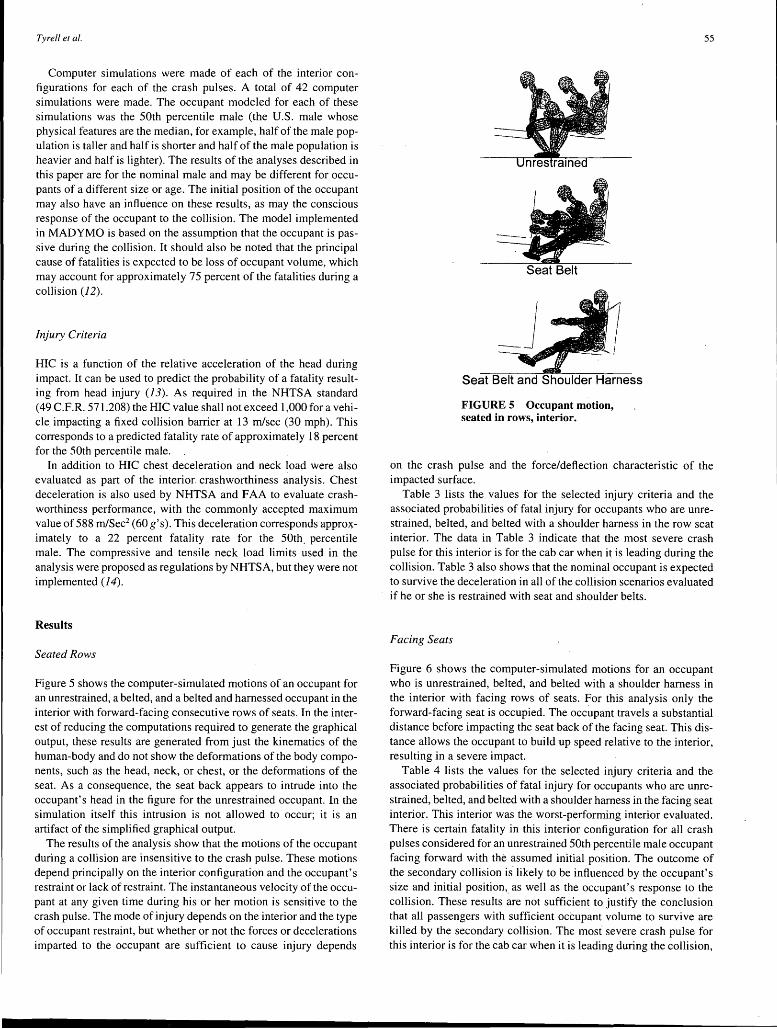
Tyrell et al.

Computer simulations were made of each of the interior con­figurations for each of the crash pulses. A total of 42 computer simulations were made. The occupant modeled for each of these simulations was the 50th percentile male (the U.S. male whose physical features are the median, for example, half of the male pop­ulation is taller and half is shorter and half of the male population is heavier and half is lighter). The results of the analyses described in this paper are for the nominal male and may be different for occu­pants of a different size or age. The initial position of the occupant may also have an influence on these results, as may the conscious response of the occupant to the collision. The model implemented in MADYMO is based on the assumption that the occupant is pas­sive during the collision. It should also be noted that the principal cause of fatalities is expected to be loss of occupant volume, which may account for approximately 75 percent of the fatalities during a collision (12).

Injury Criteria

HIC is a function of the relative acceleration of the head during impact. It can be used to predict the probability of a fatality result­ing from head injury (13). As required in the NHTSA standard ( 49 C.F.R. 571.208) the HIC value shall not exceed 1,000 for a vehi­cle impacting a fixed collision barrier at 13 m/sec (30 mph). This corresponds to a predicted fatality rate of approximately 18 percent for the 50th percentile male.

In addition to HIC chest deceleration and neck load were also evaluated as part of the interior crashworthiness analysis. Chest deceleration is also used by NHTSA and FAA to evaluate crash­worthiness performance, with the commonly accepted maximum value of 588 m/Sec2 (60 g's). This deceleration corresponds approx­imately to a 22 percent fatality rate for the 50th. percentile male. The compressive and tensile neck load limits used in the analysis were proposed as regulations by NHTSA, but they were not implemented (14).

Results

Seated Rows

Figure 5 shows the computer-simulated motions of an occupant for an unrestrained, a belted, and a belted and harnessed occupant in the interior with forward-facing consecutive rows of seats. In the inter­est of reducing the computations required to generate the graphical output, these results are generated from just the kinematics of the human-body and do not show the deformations of the body compo­nents, such as the head, neck, or chest, or the deformations of the seat. As a consequence, the seat back appears to intrude into the occupant's head in the figure for the unrestrained occupant. In the simulation itself this intrusion is not allowed to occur; it is an artifact of the simplified graphical output.

The results of the analysis show that the motions of the occupant during a collision are insensitive to the crash pulse. These motions depend principally on the interior configuration and the occupant's restraint or lack of restraint. The instantaneous velocity of the occu­pant at any given time during his or her motion is sensitive to the crash pulse. The mode of injury depends on the interior and the type of occupant restraint, but whether or not the forces or decelerations imparted to the occupant are sufficient to cause injury depends

Seat Belt and Shoulder Harness

FIGURE 5 Occupant motion, seated in rows, interior.

55

on the crash pulse and the force/deflection characteristic of the impacted surface.

Table 3 lists the values for the selected injury criteria and the associated probabilities of fatal injury for occupants who are unre­strained, belted, and belted with a shoulder harness in the row seat interior. The data in Table 3 indicate that the most severe crash pulse for this interior is for the cab car when it is leading during the collision. Table 3 also shows that the nominal occupant is expected to survive the deceleration in all of the collision scenarios evaluated if he or she is restrained with seat and shoulder belts.

Facing Seats

Figure 6 shows the computer-simulated motions for an occupant who is unrestrained, belted, and belted with a shoulder harness in the interior with facing rows of seats. For this analysis only the forward-facing seat is occupied. The occupant travels a substantial distance before impacting the seat back of the facing seat. This dis­tance allows the occupant to build up speed relative to the interior, resulting in a severe impact.

Table 4 lists the values for the selected injury criteria and the associated probabilities of fatal injury for occupants who are unre­strained, belted, and belted with a shoulder harness in the facing seat interior. This interior was the worst-performing interior evaluated. There is certain fatality in this interior configuration for all crash pulses considered for an unrestrained 50th percentile male occupant facing forward with the assumed initial position. The outcome of the secondary collision is. likely to be influenced by the occupant's size and initial position,_ as well as the occupant's response to the collision. These results are not sufficient to justify the conclusion that all passengers with sufficient occupant volume to survive are killed by the secondary collision. The most severe crash pulse for this interior is for the cab car when it is leading during the collision,

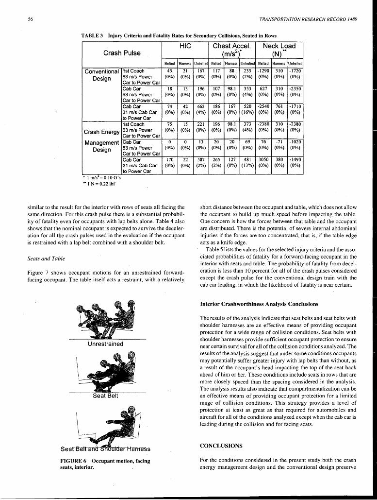
56 TRANSPORTATION RESEARCH RECORD 1489

TABLE 3 Injury Criteria and Fatality Rates for Secondary Collisions, Seated in Rows

Crash Pulse

Conventional Design

Crash Energy

Management Design

. ~ - , 1 mis -0.lOG s

** IN.= 0.22 !bf

1st Coach 63 mis Power Car to Power Car Cab Car 63 mis Power Car to Power Car Cab Car 31 mis Cab Car to Power Car 1st Coach 63 m/s Power Car to Power Car Cab Car 63 mis Power Car to Power Car Cab Car 31 mis Cab Car to Power Car

HIC

Belted Harness

45 21 (0%) (0%)

18 13 (0%) (0%)

74 42 (0%) (0%)

75 15 (0%) (0%)

0 0 (0%) (0%)

170 22 (0%) (0%)

similar to the result for the interior with rows of seats all facing the same direction. For this crash pulse there is a substantial probabil­ity of fatality even for occupants with lap belts alone. Table 4 also shows that the nominal occupant is expected to survive the deceler­ation for all the crash pulses used in the evaluation if the occupant is restrained with a lap belt combined with a shoulder belt.

Seats and Table

Figure 7 shows occupant motions for an unrestrained forward­facing occupant. The table itself acts a restraint, with a relatively

Unrestrained

Seat Belt

Sea

FIGURE 6 Occupant motion, facing seats, interior.

Chest Accel. Neck Load (m/s2f (N) **

Unbelted Belted Harness Unbelted Belted Harness Unbelted

167 117 88 235 -1290 310 -1720 (0%) (0%) (0%) (2%) (0%) (0%) (0%)

196 107 98.l 353 627 310 -2350 (0%) (0%) (0%) (4%) (0%) (0%) (0%)

662 186 167 520 -2540 761 -1710 (4%) (0%) (0%) {16%) (0%) (0%) (0%)

221 196 98.l 373 -2380 310 -2380 (0%) (0%) (0%) (4%) (0%) (0%) (0%)

13 20 20 69 76 -71 -1020 (0%) (0%) (0%) (0%) (0%) (0%) (0%)

587 265 127 481 3050 380 -1490 (2%) (2%) (0%) (13%) (0%) (0%) (0%)

short distance between the occupant and table, which does not allow the occupant to build up much speed before impacting the table. One concern is how the forces between that table and the occupant are distributed. There is the potential of severe internal abdominal injuries if the forces are too concentrated, that is, if the table edge acts as a knife edge.

Table 5 lists the values for the selected injury criteria and the asso­ciated probabilities of fatality for a forward-facing occupant in the interior with seats and table. The probability of fatality from decel­eration is less than I 0 percent for all of the crash pulses considered except the crash pulse for the conventional design train with the cab car leading, in which the likelihood of fatality is near certain.

Interior Crashworthiness Analysis Conclusions

The results of the analysis indicate that seat belts and seat belts with shoulder harnesses are an effective means of providing occupant protection for a wide range of collision conditions. Seat belts with shoulder harnesses provide sufficient occupant protection to ensure near certain survival for all of the collision conditions analyzed. The results of the analysis suggest that under some conditions occupants may potentially suffer greater injury with lap belts than without, as a result of the occupant's head impacting the top of the seat back ahead of him or her. These conditions include seats in rows that are more closely spaced than the spacing considered in the analysis. The analysis results also indicate that compartmentalization can be an effective means of providing occupant protection for a limited range of collision conditions. This strategy provides a level of protection at least as great as that required for automobiles and aircraft for all of the conditions analyzed except when the cab car is leading during the collision and for facing seats.

CONCLUSIONS

For the conditions considered in the present study both the crash energy management design and the conventional design preserve

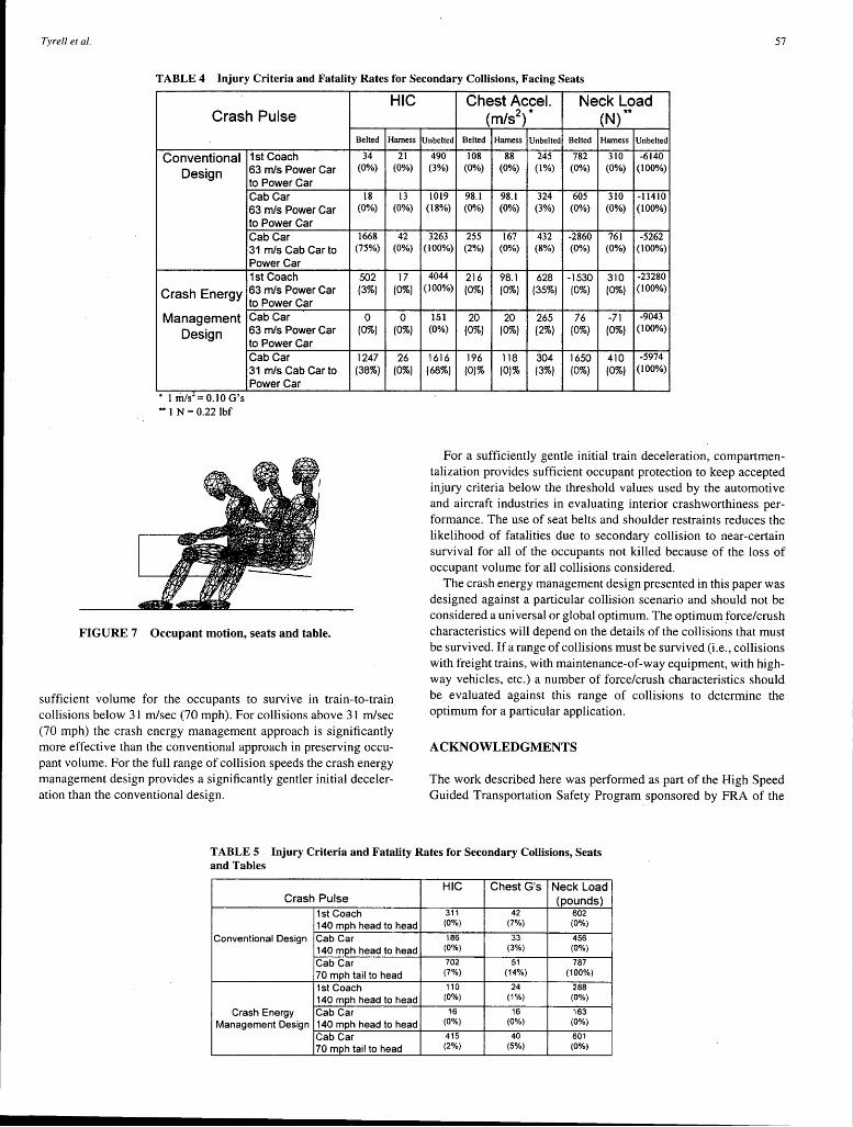
Tyrell et al. 57

TABLE 4 Injury Criteria and Fatality Rates for Secondary Collisions, Facing Seats

HIC Crash Pulse

Belted Harness

Conventional Design

Crash Energy

Management Design

. .~ -1 rills - 0.10 Gs -1 N=0.22 lbf

1st Coach 63 mis Power Car to Power Car Cab Car 63 mis Power Car to Power Car Cab Car 31 mis Cab Car to Power Car 1st Coach 63 mis Power Car to Power Car Cab Car 63 mis Power Car to Power Car Cab Car 31 mis Cab Car to Power Car

FIGURE 7 Occupant motion, seats and table.

34 (0%)

18 (0%)

1668 (75%)

502 (33)

0 (03)

1247 (383)

sufficient volume for the occupants to survive in train-to-train collisions below 31 m/sec (70 mph). For collisions above 31 m/sec (70 mph) the crash energy management approach is significantly more effective than the conventional approach in preserving occu­pant volume. For the full range of collision speeds the crash energy management design provides a significantly gentler initial deceler­ation than the conventional design.

21 (0%)

13 (0%)

42 (0%)

17 (03)

0 (03)

26 (03)

Chest Accel. Neck Load (m/s2)* (N) **

Unbelted Belted Harness Unbelted Belted Harness Unbelted

490 108 88 245 782 310 -6140 (3%) (0%) (0%) (1%) (0%) (0%) (100%)

1019 98.1 98.1 324 605 310 -11410 (18%) (0%) (0%) (3%) (0%) (0%) (100%)

3263 255 167 432 -2860 761 -5262 (100%) (2%) (0%) (8%) (0%) (0%) (100%)

4044 216 98.1 628 -1530 310 -23280 (100%) (03) (03) (353) (03) (03) (100%)

151 20 20 265 76 -71 -9043 (0%) (03) (03) (23) (03) (03) (100%)

1616 196 118 304 1650 410 -5974 (683) (0)3 (0)3 (33) (03) (03) (100%)

For a sufficiently gentle initial train deceleration, compartmen­talization provides sufficient occupant protection to keep accepted injury criteria below the threshold values used by the automotive and aircraft industries in evaluating interior ctashworthiness per­formance. The use of seat belts and shoulder restraints reduces the likelihood of fatalities due to secondary collision to near-certain survival for all of the occupants not killed because of the loss of occupant volume for all collisions considered.

The crash energy management design presented in this paper was designed against a particular collision scenario and should not be considered a universal or global optimum. The optimum force/crush characteristics will depend on the details of the collisions that must be survived. If a range of collisions must be survived (i.e., collisions with freight trains, with maintenance-of-way equipment, with high­way vehicles, etc.) a number of force/crush characteristics should be evaluated against this range of collisions to determine the optimum for a particular application.

ACKNOWLEDGMENTS

The work described here was performed as part of the High Speed Guided Transportation Safety Program. sponsored by FRA of the

TABLE 5 Injury Criteria and Fatality Rates for Secondary Collisions, Seats and Tables

HIC Chest G's Neck Load Crash Pulse (pounds)

1st Coach 311 42 602

140 mph head to head (0%) (7%) (0%)

Conventional Design Cab Car 186 33 456

140 mph head to head (0%) (3%) (0%)

Cab Car 702 51 787

70 mph tail to head (7%) (14%) (100%)

1st Coach 110 24 288

140 mph head to head (0%) (1%) (0%)

Crash Energy Cab Car 16 16 163

Management Design 140 mph head to head (0%) (0%) (0%)

Cab Car 415 40 601

70 mph tail to head (2%) (5%) (0%)

58

U.S. Department of Transportation. The authors thank Thomas Schultz, of the Office of Research and Development, and Thomas Peacock and Rolf Mowatt-Larssen, of the Office of Safety, for their assistance in developing the force/crush characteristic of the con­ventional design train and the constraints for the force/crush char­acteristics for the crash energy management design train. The authors also thank Tom Hollowell, of NHTSA's Safety Systems Engineering and Analysis Division, for the use of the MADYMO simulation program and John Guglielmi and Larry Simeone, of the Volpe Center's Crashworthiness Division, for their assistance in exercising MADYMO. Finally, the authors thank Herbert Wein­stock, of the Volpe Center's Structures and Dynamics Division, for the many helpful discussions on the modeling of dynamic systems.

REFERENCES

I. Galganski, R. A. Collision Avoidance and Accident Survivability, Vol. 3. Accident Survivability. Report DOT/FRNORD-93/02.III. FRA, U.S. Department of Transportation, March 1993.

2. Ohnishi, T., N. Kawakami, and A. Sano. Crashworthiness of Train. Proc., The International Conference on Speedup Technology for Railway and Maglev Vehicles, Vol. I, PS2-15. Japanese Society of Mechanical Engineers, Nov. 1993.

3. Lacote, F., L.-M. Cleon, H. Lagneau, M. Dannawi, E. Demonsant, and A. Wiart. Les Tolerances a la Collision Des Materials Ferroviaires. Revue Generate des Chemin de Fer. Gauthier-Villars, Nov. 1993

4. Scott, G. A. The Development of a Theoretical Technique for Rail Vehicle Structural Crashworthiness. Proc., Institute of Mechanical Engineers, Vol. 201, No. D2, 1987.

TRANSPORTATION RESEARCH RECORD 1489

5. Scholes, A. Railway Passenger Vehicle Design Loads and Structural Crashworthiness. Proc., Institute of Mechanical Engineers, Vol. 201, No. D3, 1987.

6. Scholes, A., and J. Lewis. Development of Crashworthiness for Rail­way Vehicle Structures. Proc., Institute of Mechanical Engineers, Vol. 207 Part F. Journal of Rail and Rapid Transit, 1993.

7. Romeo, D., and R. Cas·sidy. Interim Report on Assessment of Crash­worthiness of Existing Urban Rail Vehicles. Report DOT-TSC-681. Research and Speeial Programs Administration, U.S. Department of Transportation, April 1974.

8. Human Tolerance to Impact Conditions as Related to Motor Vehicle Design. SAE J885. Society of Automotive Engineers, July 1986.

9. School Bus Seating and Crash Protection. 49 C.F.R. 571, Ch. V (10-1-93 Edition), Standard No. 222.

10. Federal Motor Vehicle Safety Standards; School Bus Passenger Seating and Crash Protection; Termination of Rulemaking. Federal Register, Vol. 54, No. 54, March 22, 1989, p. 11765.

11. Lupker, H. A., P. J. A. De Coo, J. J. Neiboer, and J. Wismans. Advances in MADYMO Crash Simulations. Side Impact Occupant Protection Technologies. Publication SP-851. Society of Automotive Engineers International, Warrendale, Pa., 1991.

12. Reilly, M. J., R.H. Jines, and A. E. Tanner. Rail Safety/Equipment Crashworthiness, Vol. I. A Systems Analysis of Injury Minimization in Rail Systems. Report FRNORD-77173, I. FRA, U.S. Department of Transportation, July 1978.

13. Prasad, P., and H. Mertz. The Position of the U.S. Delegation to the ISO Working Group 6 on the Use of HIC in the Automotive Environment. SAE Paper 85-1246. Society of Automotive Engineers, 1985.

14. Pike, J. A. Automotive Safety: Anatomy, Injury, Testing and Regulation. Society of Automotive Engineers, 1990.

Publication of this paper sponsored by Committee on Guided Intercity Passenger Transportation.

TRANSPORTATION RESEARCH RECORD 1489 59

Strategic Environmental Assessment of European High-Speed Train Network

ANN DOM

To ensure the objectives of a sustainable transport policy the European Com.mission intends to apply strategic environmental assessment as an integral part of the decision-making process for transport infrastructure policies and for the trans-European networks in particular. An overview of the results of a study on the environmental impact of the European high-speed train (HST) network is provided. The study was conducted by the research and consulting group Mens en Ruimte on behalf of the Directorate-General of Transport of the European Commission. The aim of the study was (a) to make a strategic assessment of the environ­mental impact of the European HST network and (b) to compare this with the impact of the conventional modes oflong-distance transport of passengers (i.e., motorways, conventional rail, and aviation). The HST network studied corresponds to the master plan drafted by the European Commission. This plan has been drawn up with a view to the year 20 I 0 anq comprises the 12 member states, Austria, and Switzerland. In all, the network consists of ±9800 km of new lines able to cope with trains with speeds of up to 300 km/hr and ± 14 400 km of upgraded old lines to handle trains with speeds of 200 km/hr and more. Environment has been inteq)reted in the broadest sense. The themes that are considered in particl!lar are spatial impact (i.e., land use, barrier effects, impact on landscape and sensitive sites, and effects on the spatial organization of activities and on the urban environment), primary energy consumption, air pollution, noise pollution, and traffic safety. The evaluation of the influence of the HST network is performed by comparing scenarios with and without the HST network. The analysis relates to the year 20 I 0, with 1988 as the base year.

To ensure the objectives of a sustainable transport policy the European Commission intends to apply strategic environmental assessment as an integral part of the decision-making process for transport infrastructure policies, plans, and programs and for trans­European transport networks in particular (1). In the present paper an overview of the results of a study on the environmental impact of the European high-speed train (HST) network is provided. The study has been conducted by the research and consulting group Mens en Ruimte (M + R) on behalf of the Directorate-General of Transport of the European Commission (2). The main purpose is to assist the Commission in making its decisions concerning the construction of the network and the development of HSTs and to provide the basis for coordinating the efforts of the member states and for guiding their national planning.

NETWORKS AND SCENARIOS

In the present study a strategic and comparative assessment was made. The assessment was of the environmental effects of the Euro­pean HST network and the conventional modes that are used for the long-distance transport of passengers, that is, rail, road, and air transport, on networks that are in competition with the HST net-

Mens en Ruimte, Hallepoortlaan 33, B-1060 Brussels, Belgium.

work. The HST network studied corresponds to the master plan pro­posed by the Commission (Figure 1) (3). This plan has been drawn up with a view to the year 2010 and comprises the 12 member states, Austria, and Switzerland. In all the network consists of ±9800 km of new lines able to cope with trains with speeds of up to 300 km/hr and ± 14 400 km of upgraded old lines to handle trains with speeds of 200 km/hr and more. The classic rail way network ( ± 25 000 km) includes the existing interregional connections by classic trains with speeds ranging from 160 to 200 km/hr. The French TGV Sud-Est (Paris-Lyon), that is, the only high-speed line that was operational in 1988, is also included in this network ( 430 km). For road trans­port a network of main roads (mostly motorways) parallel to the HST lines has been selected (total length, ±31 450 km). For air transport a selection of 83 airports with regular intra-European commercial flights was made.

The analysis relates to the year 2010, with 1988 as the base year (the choice of 1988 was based on the availability of traffic data). The evaluation of the influence of the HST network was performed by comparing the scenarios with and without the HST network. The following scenarios were chosen:

• The 2010 Reference Scenario (2010 REF) corresponds to the situation in which no new HST lines are constructed and in which only the 1988 operational HST lines are included (i.e., Paris-Lyons).

• The 2010 High-Speed Train scenario (2010 HST) involves the complete realization of the HST network as it is proposed by the European Commission.

• The 2010 Forced Mobility scenario (2010 FM) has the same high mobility level as the 2010 HST scenario, but all traffic is achieved by using conventional traffic modes only.

TRAFFIC FLOWS

Traffic data and forecasts were derived from a study on traffic flows that was carried out by a consortium comprising INRETS (France) and INTRAPLAN (Germany) (4). That study analyzed the conse­quences of the completed network in terms of both traffic patterns and traffic growth distribution between the different modes operat­ing on the market.

Following the completion of the HST network in 2010 the long­distance transport of passengers on the selected networks will amount to almost 924 billion passenger-km (pkm) (Figure 2). A small part of this (26 billion pkm) is induced mobility, that is, traf­fic generated by the HST network itself. This newly generated traf­fic is an immediate result of the fact that with the HST network jour­neys over long distances will become more attractive. The HST network will also cause important shifts between modes: rail traffic

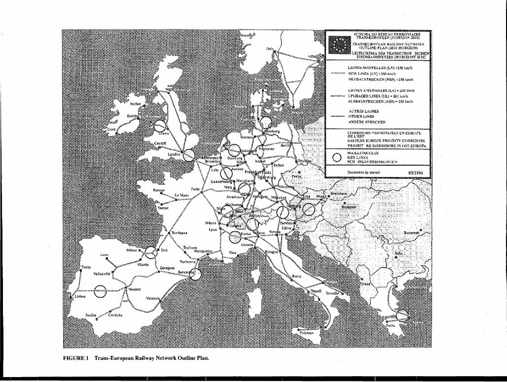
0

FIGURE 1 Trans-European Railway Network Outline Plan.

LmNC!i NOtJVEl.1...£$ (LN'j ;i.z50 km/h

NF:WUNfJ« (U\) >2Stl km/h

NIWBAl!STROCKEN (NBS) >251} km/h

LW~L'.S A:\tBNAGBJ£S (LA)"' ,Wil kmlh

t:PURADEO LINES (UL).;. ZOO km/h ACMMUSl'RECKEN (ABS)"" 1()0 km/h

AO'rRBS l..lGNES OTHERLJNES

ANDERE'. ~TllECKEN

COiUUl.lOt~S l'!tlOIU'li\JRl.S L;;N CU!Wl'E DEL'EST EASTERN EUROPE !'nl()RffV COR.RJDO!t.'! PRIOR!T RE KORRtOOfH; lN OST·EUROPA

MA.ILLO:'llS·Ct!:'.S l<£Y LJ;.(KS SCH SS!:;LV!tRUINOUN{;t;;-,;

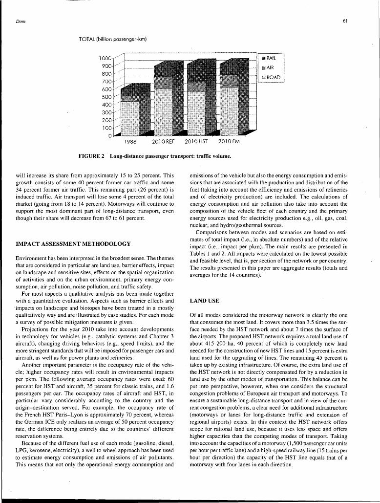
Dom

TOTAL (billion passenger-km)

l~~~f /·~--.. ---600·[/'

soo4·,,, 400{··

3001' 200·-·

100 Q.i--===

1988 2010 REF

61

·····················-·-·-·-····

-t1 MRAIL l ll~AIR ! i I j r~~R_O_A_~\

2010 HST 2010 FM

FIGURE 2 Long-distance passenger transport: traffic volume.

will increase its share from approximately 15 to 25 percent. This growth consists of some 40 percent former car traffic and some 34 percent former air traffic. This remaining part (26 percent) is induced traffic. Air transport will lose some 4 percent of the total market (going from 18 to 14 percent). Motorways will continue to support the most dominant part of long-distance transport, even though their share will decrease from 67 to 61 percent.

IMPACT ASSESSMENT METHODOLOGY

Environment has been interpreted in the broadest sense. The themes that are considered in particular are land use, barrier effects, impact on landscape and sensitive sites, effects on the spatial organization of activities and on the urban environment, primary energy con­sumption, air pollution, noise pollution, and traffic safety.

For most aspects a qualitative analysis has been made together with a quantitative evaluation. Aspects such as barrier effects and impacts on landscape and biotopes have been treated in a mostly qualitatively way and are illustrated by case studies. For each mode a surve)' of possible mitigation measures is given.

Projections for the year 2010 take into account developments in technology for vehicles (e.g., catalytic systems and Chapter 3 aircraft), changing driving behaviors (e.g., speed limits), and the more stringent standards that will be imposed for passenger cars and aircraft, as well as for power plants and refineries.

Another important parameter is the occupancy rate of the vehi­cle; higher occupancy rates will result in environmental impacts per pkm. The following average occupancy rates were used: 60 percent for HST and aircraft, 35 percent for classic trains, and 1.6 passengers per car. The occupancy rates of aircraft and HST, in particular vary considerably according to the country and the origin-destination served. For example, the occupancy rate of the French HST Paris-Lyon is approximately 70 percent, whereas the German ICE only realizes an average of 50 percent occupancy rate, the difference being entirely due to the countries' different reservation systems.

Because of the different fuel use of each mode (gasoline, diesel, LPG, kerosene, electricity), a well to wheel approach has been used to estimate energy consumption and emissions of air pollutants. This means that not only the operational energy consumption and

emissions of the vehicle but also the energy consumption and emis­sions that are associated with the production and distribution of the fuel (taking into account the efficiency and emissions of refineries and of electricity production) are included. The calculations of energy consumption and air pollution also take into account the composition of the vehicle fleet of each country and the primary energy sources used for electricity production e.g., oil, gas, coal, nuclear, and hydro/geothermal sources.

Comparisons between modes and scenarios are based on esti­mates of total impact (i.e., in absolute numbers) and of the relative impact (i.e., impact per pkm). The main results are presented in Tables 1 and 2. All impacts were calculated on the lowest possible and feasible level, that is, per section of the network or per country. The results presented in this paper are aggregate results (totals and averages for the 14 countries).

LAND USE

Of all modes considered the motorway network is clearly the one that consumes the most land. It covers more than 3.5 times the sur­face needed by the HST network and about 7 times the surface of the airports. The proposed HST network requires a total land use of about 415 200 ha, 40 percent of which is completely new land needed for the construction of new HST lines and 15 percent is extra land used for the upgrading of lines. The remaining 45 percent is taken up by existing infrastructure. Of course, the extra land use of the HST network is not directly compensated for by a reduction in land use by the other modes of transportation. This balance can be put into perspective, however, when one considers the structural congestion problems of European air transport and motorways. To ensure a sustainable long-distance transport and in view of the cur­rent congestion problems, a clear need for additional infrastructure (motorways or lanes for long-distance traffic and extension of regional airports) exists. In this context the HST network offers scope for rational land use, because it uses less space and offers higher capacities than the competing modes of transport. Taking into account the capacities of a motorway (1,500 passenger car units per hour per traffic lane) and a high-speed railway line (15 trains per hour per direction) the capacity of the HST line equals that of a motorway with four lanes in each direction.

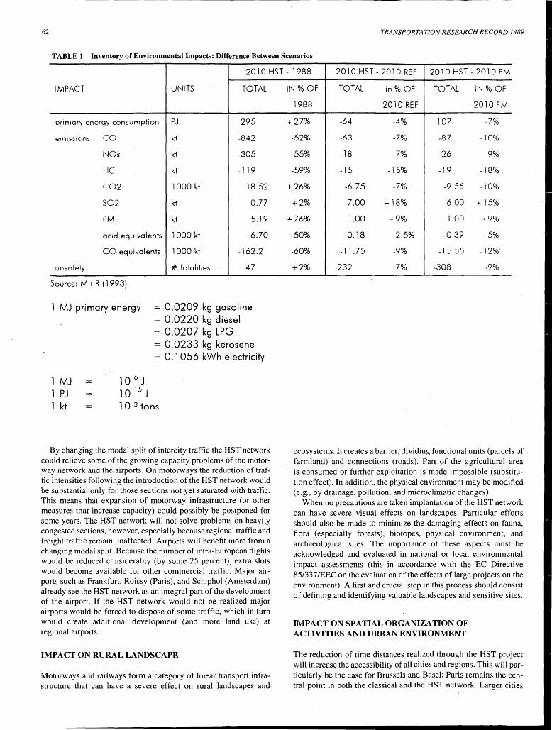
62 TRANSPORTATION RESEARCH RECORD 1489

TABLE 1 Inventory of Environmental Impacts: Difference Between Scenarios

2010 HST - 1988 2010 HST - 2010 REF 2010 HST - 2010 FM

IMPACT UNITS TOTAL

primary energy consumption PJ 295

emissions co kt -842

NOx kt -305

HC kt -119

C02 1000 kt 18.52

S02 kt 0.77

PM kt 5.19

acid equivalents 1000 kt -6.70

CO equivalents 1000 kt -162.2

unsafety # fatalities 47

Source: M + R ( 1993)

1 MJ primary energy = 0.0209 kg gasoline = 0.0220 kg diesel

1 MJ 1 PJ 1 kt

= 0.0207 kg LPG = 0.0233 kg kerosene = 0.1 056 kWh electricity

10 6 J 10 15 J 10 3 tons

By changing the modal split of intercity traffic the HST network could relieve some of the growing capacity problems of the motor­way network and the airports. On motorways the reduction of traf­fic intensities following the introduction of the HST network would be substantial only for those sections not yet saturated with traffic. This means that expansion of motorway infrastructure (or other measures that increase capacity) could possibly be postponed for some years. The HST network will not solve problems on heavily congested sections, however, especially because regional traffic and freight traffic remain unaffected. Airports will benefit more from a changing modal split. Because the number of intra-European flights would be reduced considerably (by some 25 percent), extra slots would become available for other commercial traffic. Major air­ports such as Frankfurt, Roissy (Paris), and Schiphol (Amsterdam) already see the HST network as an integral part of the development of the airport. If the HST network would not be realized major airports would be forced to dispose of some traffic, which in. turn would create additional development (and more land. use) at regional airports.

IMPACT ON RURAL LANDSCAPE

Motorways and railways form a category of linear transport infra­structure that can have a severe effect on rural landscapes and

IN%0F TOTAL in% OF TOTAL IN%0F

1988 2010 REF 2010 FM

+27% -64 -4% -107 -7%

-52% -63 -7% -87 -10%

-55% -18 -7% -26 -9%

-59% -15 -15% -19 -18%

+26% -6.75 -7% -9.56 -10%

+2% 7.00 + 18% 6.00 +15%

+76% 1.00 +9% 1.00 +9%

-50% -0.18 -2.5% -0.39 -5%

-60% -11.75 -9% -15.55 -12%

+2% -232 -7% -308 -9%

ecosystems. It creates a barrier; dividing functional units (parcels of farmland) and connections (roads). Part of the agricultural area is consumed or further exploitation is made impossible (substitu­tion effect). In addition, the physical environment may be modified (e.g., by drainage, pollution, and microclimatic changes).

When no precautions are taken implantation of the HST network can have severe visual effects on landscapes. Particular efforts should also be made to minimize the damaging effects on fauna, flora (especially forests), biotopes, physical environment, and archaeological sites. The importance of these aspects must be acknowledged and evaluated in national or local environmental impact assessments (this in accordance with the EC Directive 85/337 /EEC on the evaluation of the effects of large projects on the environment). A first and crucial step in this process should consist of defining and identifying valuable landscapes and sensitive sites.

IMPACT ON SPATIAL ORGANIZATION OF ACTIVITIES AND URBAN ENVIRONMENT

The reduction of time distances realized through the HST project will increase the accessibility of all cities and regions. This will par­ticularly be the case for Brussels and Basel; Paris remains the cen­tral point in both the classical and the HST network. Larger cities

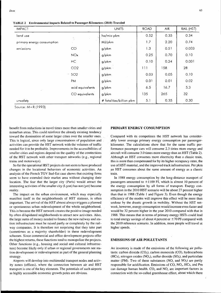
Dom 63

TABLE 2 Environmental Impacts Related to Passenger-Kilometers (2010) Traveled

IMPACT UNITS ROAD AIR RAIL (HST)

land use ha/mio pkm 0.52 0.35 0.34

primary energy consumption MJ/pkm 1.7 2.20 0.74

emissions co g/pkm l.3 0.51 0.003

NOx

HC

C02

S02

PM

acid equivalents

CO equivalents

unsafety

Source: M+ R (1993)

benefit from reductions in travel times more than smaller cities and nonurban areas. This could reinforce the already existing tendency toward the domination of some larger cities over the smaller ones. This is logical, since only large concentrations ·of population and activities can provide the HST network with the volumes of traffic needed for it to be profitable. Improvements in the accessibilities of smaller cities and regions depend on the quality of the confiectiOns of the HST network with other transport networks (e.g., regional trains and motorways). ·

So far the operational HST projects do not seem to have produced changes in the locational behaviors of economic activities. An analysis of the French TGV Sud-Est case shows that existing firms seem to have extended their market area without changing their location. The fear that the larger city (Paris) would attract the interesting activities of the smaller city (Lyon) has not (yet) become reality.

The impact on the urban environment, which may especially manifest itself in the neighborhoods of HST stations, is often important. The arrival of the HST almost always triggers a planned or spontaneous urban redevelopment of the whole neighborhood. This is because the HST network creates the positive image needed by often dilapidated ne_ighborhoods to attract new activities. Also, the large sums of money needed to finance the new railway and sta­tion infrastructure must be raised partly or completely by the rail­way companies. It is therefore not surprising that they take part (sometimes as a majority shareholder) in these redevelopment schemes. Since commercial and office development projects offer the highest returns, these functions tend to monopolize the projects. Other functions (e.g., housing and social and cultural infrastruc­ture) become likely only if urban or regional governments see sta­tion development or redevelopment as part of the general planning strategy.

Airports will develop into multimodal transport nodes and activ­ity zones (offices), where the connection between air and HST transport is one of the key elements. The potentials of such airports as highly accessible economic growth poles are obvious.

g/pkm 0.25 0.70 0.10

g/pkm 0.10 0.24 0.001

g/pkm 111 158 28

g/p_km 0.03 0.05 0.10

g/pkm 0.01 0.01 0.02

g/pkm 6.5 16.7 5.3

g/pkm 135 265 32

# fatalities/billion pkm 5.1 0.35 0.30

PRIMARY ENERGY CONSUMPTION

Compared with its competitors the HST network has consider­ably lower average primary energy consumption per passenger­kilometer. The calculations show that for the same traffic per­formance passenger cars will consume 2.3 tirri€s rriore energy and aircraft will consume 3.0 times more energy than an HST (Table 2). Although an HST consumes more electricity than a classic train, this is more than compe·nsated for by its higher occupancy rates, the use of HST material, and the improved track infrastructure. Per pkm _an HST consumes about the same amount of energy as a classic train.

In 1988 energy consumption by the long-distance transport of passengers amounted to ± 1109 PJ, which is almost 10 percent of the energy consumption by all forms of transport. Energy con­sumption in the 2010 HST scenario will be about 27 percent higher than that in 1988 (Table 1 and Figure 3). Even though the energy efficiency of the modes will improve this effect will be more than undone by the. drastic growth in mobility. Without the HST net­work, however, energy consumption would increase even faster and would be 32 percent higher in the year 2010 compared with that in 1988. This means that in terms of primary energy HSTs could lead to total energy savings of about 4 percent or ±70 PJ compared with the 2010 reference scenario. In addition, more people will travel at higher speeds.

EMISSIONS OF AIR POLLUTANTS.

An inventory is made of the emissions of the following air pollu­tants: carbon dioxide (C02), carbon monoxide (CO), hydrocarbons (HCs), nitrogen oxides (NQ_r), sulfur dioxide (S02), and particulate matter (PM). Two of these substances (NOx and S02) are partly responsible for acidification. Emissions of CO, NO.n HCs, and Pm can damage human health. C02 and NOx are important factors in connection with the so-called greenhouse effect, about which there

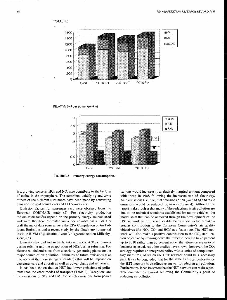
64

TOTAL (PJ)

1.988 2010 REF

RELATIVE (MJ per passenger-km}

2010 HST 2010 FM

TRANSPORTATION RESEARCH RECORD 1489

Blll RAIL

~AlR

BROAD

D:JROAD

~AIR

§!!RAIL

1988 2010 REF 2010 HST

FIGURE 3 Primary energy consumption.

is a growing concern. HCs and NO, also contribute to the buildup of ozone in the troposphere. The combined acidifying and toxic effects of the different substances have been made by converting emissions to acid equivalents and CO equivalents.

Emission factors for passenger cars were obtained from. the European CORINAIR study (5). For electricity production the emission factors depend on the primary energy sources used and· were therefore estimated on a per country basis. For air­craft the major data sources were the EPA Compilation of Air Pol­lutant Emissions and a recent study by the Dutch environmental institute RIVM (Rijksinstituut voor Volkgezondheid en Milienhy­giene) (6).

Emissions by road and air traffic take into account S02 emissions during refining and the evaporation of HCs during refueling. For electric rail the emissions from electricity-generating plants are the major source of air pollution. Estimates of future emissions take into account the more stringent standards that will be imposed on passenger cars and aircraft as well as power plants and refineries.

It has been shown that an HST has lower emissions of pollu­tants than the other modes of transport (Table 2). Exceptions are the emissions of S02 and PM, for which emissions from power

stations would increase by a relatively marginal amount compared with those in 1988 following the increased use of electricity. Acid emissions (i.e., the joint emissions of NOx and S02) and toxic emissions would be reduced, however (Figure 4). Although the report makes it clear that many of the reductions in air pollution are due to the technical standards established for motor vehicles, the modal shift that can be achieved through the development of the HST network in Europe will enable the transport sector to make a greater contribution to the European Community's air quality objectives (for N0.0 CO, and HCs) at a faster rate. The HST net­work will also make a positive contribution to the C02 stabiliza­tion objective by slowing down the forecast increase to 26 percent up to 2010 rather than 30 percent under the reference scenario of business as usual. As other studies have shown, however, the C02

strategy requires an integrated policy with a series of complemen­tary measures, of which the HST network could be a necessary part. It can be concluded that for the same transport performance the HST network is an effective answer to reducing air pollution. Furthermore, it can be stated that the HST network can make a pos­itive contribution toward achieving the Community's goals of reducing air pollution.

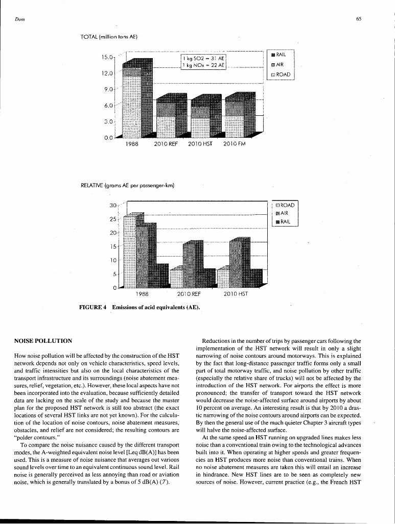
Dom 65

TOTAL (million tons AE}

l S.0

1 12.0

I 9.0f

1---- -----~~~-~-;;;:·;1-~;1----- ! [ RAO~AL D_-Jll:;

.. 1 kg NOx = 22 AE ................ ·-·-·-.. ----·

I 6.o·I

3.0

1988 2010 REF 2010 HST

RELATIVE (grams AE per passenger-km)

1988 2010 REF

2010 FM

2010 HST

EJROAD

!$!AIR

a RAIL

FIGURE 4 Emissions of acid equivalents (AE).

NOISE POLLUTION

How noise pollution will be affected by the construction of the HST network depends not only on vehicle characteristics, speed levels, and traffic intensities but also on the local characteristics of the transport infrastructure and its surroundings (noise abatement mea­sures, relief, vegetation, etc.). However, these local aspects have not been incorporated into the evaluation, because sufficiently detailed data are lacking on the scale of the study and because the master plan for the proposed HST network is still too abstract (the exact locations of several HST links are not yet known). For the calcula­tion of the location of noise contours, noise abatement measures, obstacles, and relief are not considered; the resulting contours are "polder contours."

To compare the noise nuisance caused by the different transport modes, the A-weighted equivalent noise level [Leq dB(A)] has been used. This is a measure of noise nuisance that averages out various sound levels over time to an equivalent continuous sound level. Rail noise is generally perceived as less annoying than road or aviation noise, which is generally translated by a bonus of 5 dB(A) (7).

Reductions in the number of trips by passenger cars following the implementation of the HST network will result in only a slight narrowing of noise contours around motorways. This is explained by the fact that long-distance passenger traffic forms only a small part of total motorway traffic, and noise pollution by other traffic (especially the relative share of trucks) will not be affected by the introduction of the HST network. For airports the effect is more pronounced; the transfer of transport toward the HST network would decrease the noise-affected surface around airports by about 10 percent on average. An interesting result is that by 20 I 0 a dras­tic narrowing of the noise contours around airports can be expected. By then the general use of the much quieter Chapter 3 aircraft types will halve the noise-affected surface.

At the same speed an HST running on upgraded lines makes less noise than a conventional train owing to the technological advances built into it. When operating at higher speeds and greater frequen­cies an HST produces more noise than. conventional trains. When no noise abatement measures are taken this will entail an increase in hindrance. New HST lines are to be seen as completely new sources of noise. However, current practice (e.g., the French HST

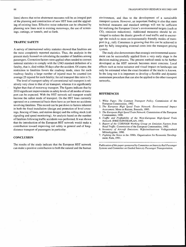
66

lines) shows that noise abatement measures will be an integral part of the planning and construction of new HST lines and the upgrad­ing of existing lines. Effective noise reduction can be obtained by planning new lines next to existing motorways, the use of screen­ings, cuttings, or tunnels, and so forth.

TRAFFIC SAFETY

A survey of international safety statistics showed that fatalities are the most completely reported statistics. Thus, the analysis in the present study focused on calculating the number of fatalities among passengers. Correction factors were applied when needed to convert national statistics to comply with the UNO standard definition of a fatality, that is, died within 30 days after the accident. Of course, the restriction to fatalities favors the roadway mode, since for each roadway fatality a large number of injured must be counted (on average 25 injured for each fatality; for rail transport this ratio is 3).

The level of transport safety of conventional rail transport is rel­atively very close to that of air transport, whereas it is significantly higher than that of motorway transport. The figures indicate that by 2010 significant improvements in safety levels of all modes of trans­port can be expected. With the HST network rail transport would become the safest mode of transport. On the HST lines currently operated on a commercial basis there have as yet been no accidents involving fatalities. This record can be put down to factors inherent in both the fixed installation (design and protection of level cross­ings, fencing of lines, and station design) and the rolling stock (cab signaling and speed monitoring). An analysis based on the number of fatalities following traffic accidents was performed. It was shown that the introduction of the European HST network would make a_ contribution toward improving rail safety in general and of long­distance transport of passengers in particular.

CONCLUSION

The results of the study indicate that the European HST network can make a positive contribution to both the natural and the human

TRANSPORTATION RESEARCH RECORD 1489

environment, and thus to the development of a sustainable transport system. However, an important finding is also that mere technical measures and standard settings will not be sufficient for realizing the European Union's environmental targets (such as C02 emission reductions). Additional measures should be en­visaged to reduce the drastic growth of road traffic and to encour­age the switch to more environmentally friendly modes of trans­port (e.g., rail). Consensus is growing that this can be achieved in part by fully integrating external costs into the transport pricing system.

The study also demonstrates that strategic environmental assess­ment can be successfully applied from a very early stage in the decision-making process. The present method needs to be further developed as the HST network becomes more concrete. Local effects such as noise nuisance and visual impact on landscape can only be estimated when the exact location of the tracks is known. In the long run it is important to develop a flexible and dynamic assessment procedure that can also be applied to the other transport networks.

REFERENCES

1. White Paper, The Common Transport Policy. Commission of the European Communities, 1992.

2. The European High Speed Train Network: Environmental Impact Assessment. Mens en Ruimte, Brussels, 1993.

3. The European High Speed Train Network. Commission of the European Communities, 1990.

4. Traffic and Profitability of the West-European High-Speed Train Network. INRETS/INTRAPLAN, 1993.

5. Report of the CORINAIR Working Group on Emission Factors from Road Traffic. Commission of the European Communities, 1992.

6. Inventory of Aircraft Emissions. Rijksinstituutvoor Volkgezonheid Milienhygiene, 1990.

7. Fighting the Noise in the I990s. Organization for Economic Develop­ment, Paris, 1991.

Publication of this paper sponsored by Committee on Intercity Rail Passenger Systems and Committee on Guided Intercity Passenger Transportation.

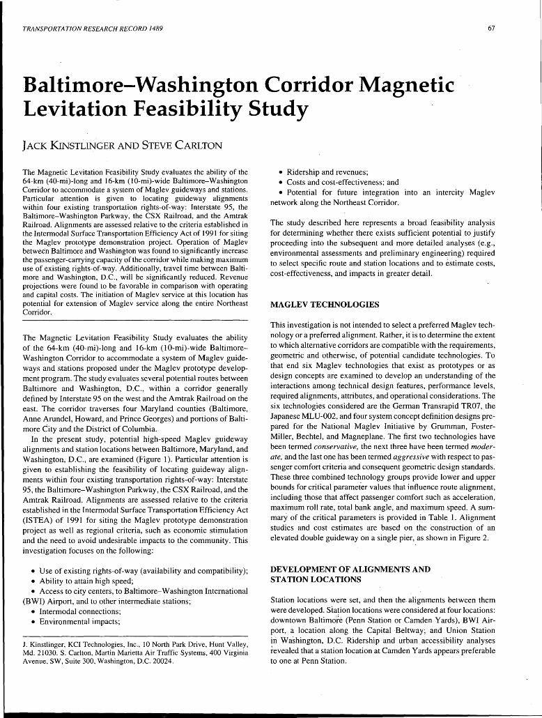
TRANSPORTATION RESEARCH RECORD 1489 67

Baltimore-Washington Corridor Magnetic Levitation Feasibility Study

JACK KINSTLINGER AND STEVE CARLTON

The Magnetic Levitation Feasibility Study evaluates the ability of the 64-km (40-mi)-long and 16-km (10-mi)-wide Baltimore-Washington Corridor to accommodate a system of Maglev guideways and stations. Particular attention is given to locating guideway alignments within four existing transportation rights-of-way: Interstate 95, the Baltimore-Washington Parkway, the CSX Railroad, and the Amtrak Railroad. Alignments are assessed relative to the criteria established in the Intermodal Surface Transportation Efficiency Act of 1991 for siting the Maglev prototype demonstration project. Operation of Maglev between Baltimore and Washington was found to significantly increase the passenger-carrying capacity of the corridor while making maximum use of existing rights-of-way. Additionally, travel time between Balti­more and Washington, D.C., will be significantly reduced. Revenue projections were found to be favorable in comparison with operating and capital costs. The initiation of Maglev service at this location has potential for extension of Maglev service along the entire Northeast Corridor.

The Magnetic Levitation Feasibility Study evaluates the ability of the 64-km ( 40-mi)-long and 16-km (10-mi)-wide Baltimore­Washington Corridor to accommodate a system of Maglev guide­ways and stations proposed under the Maglev prototype d~velop­ment program. The study evaluates several potential routes between Baltimore and Washington, D.C., within a corridor generally defined by Interstate 95 on the west and the Amtrak .Railroad on the east. The corridor traverses four Maryland counties (Baltimore, Anne Arundel, Howard, and Prince Georges) and portions of Balti­more City and the District of Columbia.

In the present study, potential high-speed Maglev guideway alignments and station locations between Baltimore, Maryland, and Washington, D.C., are examined (Figure I). Particular attention is given to establishing the feasibility of locating guideway align­ments within four existing transportation rights-of-way: Interstate 95, the Baltimore-Washington Parkway, the CSX Railroad, and the Amtrak Railroad. Alignments are assessed relative to the criteria established in the Intermodal Surface Transportation Efficiency Act (ISTEA) of 1991 for siting the Maglev prototype demonstration project as well as regional criteria, such as economic stimulation and the need to avoid undesirable impacts to the community. This investigation focuses on the following:

• Use of existing rights-of-way (availability and compatibility); • Ability to attain high speed; • Access to city centers, to Baltimore-Washington International

(BWI) Airport, and to other intermediate stations; • Intermodal connections; • Environmental impacts;

J. Kinstlinger, KCI Technologies, Inc., 10 North Park Drive, Hunt Valley, Md. 21030. S. Carlton, Martin Marietta Air Traffic Systems, 400 Virginia Avenue, SW, Suite 300, Washington, D.C. 20024.

• Ridership and revenues; • Costs and cost-effectiveness; and • Potential for future integration into an intercity Maglev

network along the Northeast Corridor.

The study described here represents a broad feasibility analysis for determining whether there exists sufficient potential to justify proceeding into the subsequent and more detailed analyses (e.g., environmental assessments and preliminary engineering) required to select specific route and station locations and to estimate costs, cost-effectiveness, and impacts in greater detail.

MAGLEV TECHNOLOGIES

This investigation is not intended to select a preferred Maglev tech­nology or a preferred alignment. Rather, it is to determine the extent to which alternative corridors are compatible with the requirements, geometric and otherwise, of potential candidate technologies. To that end six Maglev technologies that exist as prototypes or as design concepts are examined to develop an understanding of the interactions among technical design features, performance levels, required alignments, attributes, and operational considerations. The six technologies considered are the German Transrapid TR07, the Japanese MLU-002, and four system concept definition designs pre­pared for the National Maglev Initiative by Grumman, Foster­Miller, Bechtel, and Magneplane. The first two technologies have been termed conservative, the next three have been termed moder­ate, and the last one has been termed aggressive with respect to pas­senger comfort criteria and consequent geometric design standards. These three combined technology groups provide lower and upper bounds for critical parameter values that influence route alignment, including those that affect passenger comfort such as acceleration, maximum roll rate, total bank angle, and maximum speed. A sum­mary of the critical parameters is provided in Table 1. Alignment studies and cost estimates are based on the construction of an elevated double guideway on a single pier, as shown in Figure 2.

DEVELOPMENT OF ALIGNMENTS AND STATION LOCATIONS

Station locations were set, and then the. alignments between them were developed. Station locations were considered at four locations: downtown Baltimote (Penn Station or Camden Yards), BWI Air­port, a location along the Capital Beltway; and Union Station iri Washington, D.C. Ridership and urban accessibility analyses revealed that a station location at Camden Yards appears preferable to one at Penn s·tation.

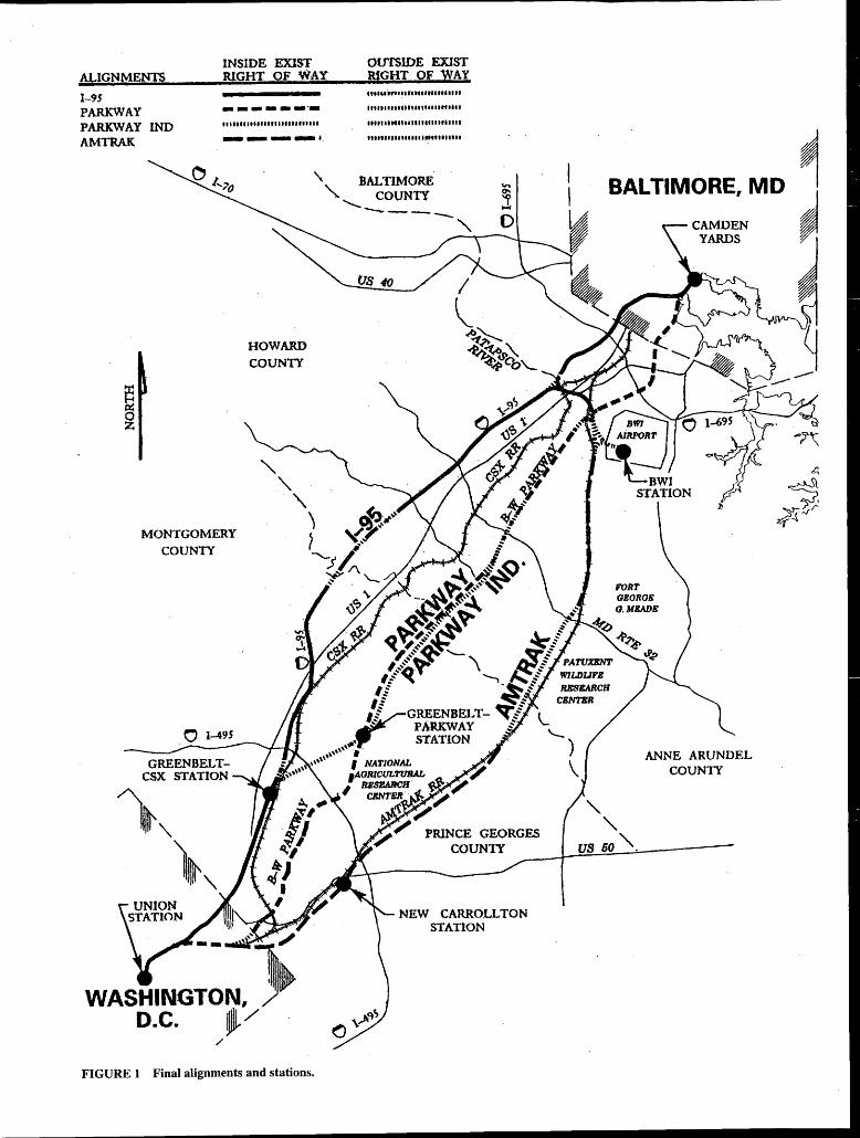
ALIGNMENTS

1-95 PARKWAY PARKWAY IND AMTRAK

INSIDE EXIST RIGHT OF WAY

------·-llltUfltlllltU Utlllfll 111 ----··

OlITSIDE EXIST RtGHT .OF WAY •tt•utn11tf1HIUHH•1111

...................... "'"' ltltlll"lltlltltHlllUllll

111n111u111111Uttttnnn

'\ BALTIMORE '-....'-..... COUNTY

~ 0 z.

MONTGOMERY COUNTY

HOWARD COUNTY

FIGURE 1 Final alignments and stations.

-...... __ ___ "

NEW CARROLLTON STATION

ANNE ARUNDEL CO UNIT

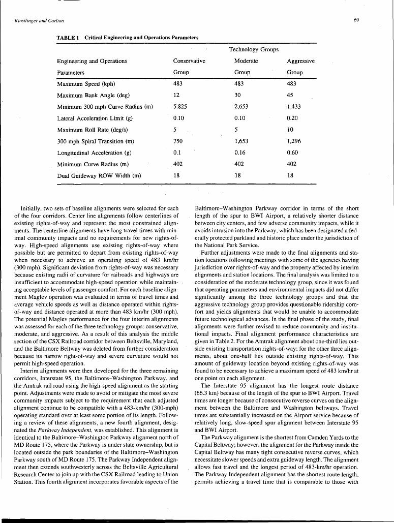
Kinstlinger and Carlton 69

TABLE 1 Critical Engineering and Operations Parameters

Technology Groups

Engineering and Operations Conservative Moderate Aggressive

Parameters

Maximum Speed (kph)

Maximum Bank Angle (deg)

Minimum 300 mph Curve Radius (m)

Lateral Acceleration Limit (g)

Maximwn Roll Rate (deg/s)

300 mph Spiral Transition (m)

Longitudinal Acceleration (g)

Minimum Curve Radius (m)

Dual Guideway ROW Width (m)

Group

483

12

5,825

0.10

5

750

0.1

402

18

Initially, two sets of baseline alignments were selected for each of the four corridors. Center line alignments follow centerlines of existing rights-of-way and represent the most constrained align­ments. The centerline alignments have long travel times with min­imal community impacts and no requirements for new rights-of­way. High-speed alignments use existing rights-of-way where possible but are permitted to depart from existing rights-of-way when necessary to achieve an operating speed of 483 km/hr (300 mph). Significant deviation from rights-of-way was necessary because existing radii of curvature for railroads and highways are insufficient to accommodate high-speed operation while maintain­ing acceptable levels of passenger comfort. For each baseline align­ment Maglev operation was evaluated in terms of travel times and average vehicle speeds as well as distance operated within rights­of-way and distance operated at more than 483 km/hr (300 mph). The potential Maglev performance for the four interim alignments was assessed for each of the three technology groups: conservative, moderate, and aggressive. As a result of this analysis the middle section of the CSX Railroad corridor between Beltsville, Maryland, and the Baltimore Beltway was deleted from further consideration because its narrow right-of-way and severe curvature would not permit high-speed operation.

Interim alignments were then developed for the three remaining corridors, Interstate 95, the Baltimore-Washington Parkway, and the Amtrak rail road using the high-speed alignment as the starting point. Adjustments were made to avoid or mitigate the most severe community impacts subject to the requirement that each adjusted alignment continue to be compatible with a 483-km/hr (300-mph) operating standard over at least some portion of its length. Follow­ing a review of these alignments, a new fourth alignment, desig­nated the Parkway Independent, was established. This alignment is identical to the Baltimore-Washington Parkway alignment north of MD Route 175, where the Parkway is under state ownership, but is located outside the park boundaries of the Baltimore-Washington Parkway south of MD Route 175. The Parkway Independent align­ment then extends southwesterly across the Beltsville Agricultural Research Center to join up with the CSX Railroad leading to Union Station. This fourth alignment incorporates favorable aspects of the

Group Group

483 483

30 45

2,653 1,433

0.10 0.20

5 10

1,653 1,296

0.16 0.60

402 402

18 18

Baltimore-Washington Parkway corridor in terms of the short length of the spur to BWI Airport, a relatively shorter distance between city centers, and few adverse community impacts, while it avoids intrusion into the Parkway, which has been designated a fed­erally protected parkland and historic place under the jurisdiction of the National Park Service.

Further adjustments were made to the final alignments and sta­tion locations following meetings with some of the agencies having jurisdiction over rights-of-way and the property affected by interim alignments and station locations. The final analysis was limited to a consideration of the moderate technology group, since it was found that operating parameters and environmental impacts did not differ significantly among the three technology groups and that the aggressive technology group provides questionable ridership com­fort and yields alignments that would be unable to accommodate future technological advances. In the final phase of the study, final alignments were further revised to reduce community and institu­tional impacts. Final alignment performance characteristics are given in Table 2. For the Amtrak alignment about one-third lies out­side existing transportation rights-of-way; for the other three align­ments, about one'"half lies outside existing rights-of-way. This amount of guideway location beyond existing rights-of-way was found to be necessary to achieve a maximum speed of 483 km/hr at one point on each alignment.

The Interstate 95 alignment has the longest route distance (66.3 km) because of the length of the spur to BWI Airport. Travel times are longer because of consecutive reverse curves on the align­ment between the Baltimore and Washington beltways. Travel times are substantially increased on the Airport service because of relatively long, slow-speed spur alignment between Interstate 95 and BWI Airport.

The Parkway alignment is the shortest from Camden Yards to the Capital Beltway; however, the alignment for the Parkway inside the Capital Beltway has many tight consecutive reverse curves, which necessitate slower speeds and extra guideway length. The alignment allows fast travel and the longest period of 483-km/hr operation. The Parkway Independent alignment has the shortest route length, permits achieving a travel time that is comparable to those with

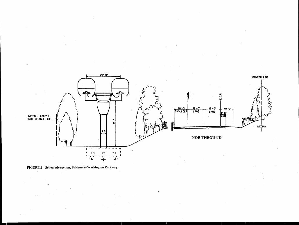
LIMITED - ACCESS _j RIGHT-OF-WAY LINE -,

I I

+•

~

4.5'

1----- ----,

I // II (\ I

' -1-, - - r r - ' -+ _J

~ ~~ :..\-

FIGURE 2 Schematic section, Baltimore-:-Washington Parkway.

CENTER LINE

10·-o· 12·-o· 12·-o· SHOULDER LANE LANE

MEDIAN I

NORTHBOUND

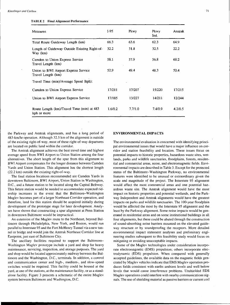
Kinstlinger and Carlton

TABLE2 Final Alignment Performance

Measures

Total Route Guideway Length (km)

Length of Guideway Outside Existing Right-of-Way (km)

Camden to Union Express Service Travel Length (km)

Union to BWI Airport Express Service Travel Length (km)

Travel Time (min)/ Average Speed (kph):

Camden to Union Express Service

Union to BWI Airport Express Service

Route Length (km)ffravel Time (min) at 483 kph or more

the Parkway and Amtrak alignments, and has a long period of 483-km/hr operation. Although 32.5 km of the alignment is outside of the existing right-of-way, most of these right-of-way departures are located on public land within the corridor.

The Amtrak alignment achieves the best travel time and highest average speed from BWI Airport to Union Station among the four alternatives. The short length of the spur from this alignment to BWI Airport compensates for the longer distance between Camden Yards and Union Station. This alignment has the shortest length (22.2 km) outside the existing right-of-way.

The final statiori locations recommended are Camden Yards in downtown Baltimore, BWI Airport, Union Station in Washington, D.C., and a future station to be located along the Capital Beltway. This future station would be needed to accommodate expected rid­ership increases in the event that the Baltimore-Washington Maglev becomes part of a larger Northeast Corridor operation, and therefore, land for this station should be acquired initially during development of the prototype stage for later development. Analy­ses have shown that constructing a spur alignment at Penn Station in downtown Baltimore would be impractical. ·

An extension of the Maglev route to the Northeast, beyond Bal­timore through Philadelphia, New York, and Boston, would run parallel to Interstate 95 and the Fort McHenry Tunnel via a new tun­nel or bridge and would join the Amtrak Northeast Corridor line at Eastpoint, just east of Baltimore City.

The ancillary facilities required to support the Baltimore­Washington Maglev .prototype include a yard and shop for heavy maintenance, servicing, inspection, and storage purposes. The yard and shop would be located approximately midway between the Bal­timore and the Washington, D.C., terminals. In addition, a control and communication center and high-, medium-, and slow-speed switches would be required. This facility could be housed at the yard, at one of the stations, at the maintenance facility, or as a stand­alone facility. Figure 3 presents a schematic of the entire Maglev system between Baltimore and Washington, D.C.

71

I-95 Pkwy Pkwy Amtrak Ind.

66.3 63.6 62.3 64.9

32.2 31.8 32.5 22.2

58.l 57.9 56.8 60.2

52.9 49.4 48.3 50.4

17 /211 17/207 151220 17/215

17/185 13/227 14/211 12/244

1.6/0.2 7.7/1.0 7.4/0.9 4.2/0.5

ENVIRONMENTAL IMPACTS

The environmental evaluation is.concerned with identifying princi­pal environmental issues that would have a major influence on cor­ridor and station feasibility and location. These issues focus on potential impacts to historic properties, hazardous waste sites, wet• lands, parks and wildlife sanctuaries, floodplains, forests, residen­tial and commercial areas, noise, and electromagnetic fields. Envi­ronmental impacts are described in Table 3. Except for the protected status of the Baltimore-Washington Parkway, no environmental features were identified to be unusual or extraordinary given the scale arid magnitude of the project. The Interstate 95 alignment Would affect the most commercial areas and one potential haz­ardous waste site. The Amtrak alignment would have the most impact on historic properties and potential wetlands, and the Park­way Independent and Amtrak alignments would have the greatest impacts on parks and wildlife sanctuaries. The 100-year floodplain would be affected the most by the Interstate 95 alignment and the least by the Parkway alignment. Some noise impacts would be gen­erated in residential areas and on some institutional buildings in all four alignments, but these could be abated through the construction of sound-absorbing noise barriers mounted on the elevated guide­way structure or by soundproofing the receptors. More detailed environmental impact statement analyses and preliminary engi­neering studies subsequent to this feasibility study would focus on mitigating or avoiding unacceptable impacts.

Some of the Maglev technologies under consideration incorpo­rate electromagnetic (EMS) propulsion; others incorporate elec­trodynamic (EDS) propulsion. When compared with generally accepted guidelines, the available data on the magnetic fields gen­erated by Maglev vehicles indicate that EMS Maglev operation pro­duces fields consistent with earths ambient levels and well below levels that would cause interference problems. Unshielded EDS Maglev operations could interfere with nearby communications sig­nals. The use of shielding material as passive barriers or current coil

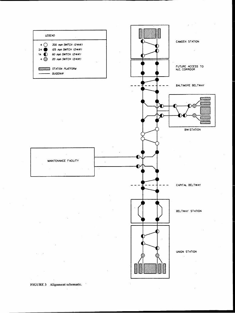
LEGEND

300 mp/I SWffCH <2-WAYJ

125 mp/I SWffCH £2-WAYJ

60 mp/I SWffCH t2-WAYJ

20 mp/I SWffCH f2:WAYJ

~ ST AT/ON PLATFORM

GUID£WAY

MArNTENANCE FACILITY

FIGURE 3 Alignment schematic.

1111

HllH

CAMDEN STATION

FUTURE ACCESS TO N.E. CORRIDOR

BALTIMORE BELTWAY

BWISTATION

CAPITAL BELTWAY

BELTWAY STATION

UNION STATION

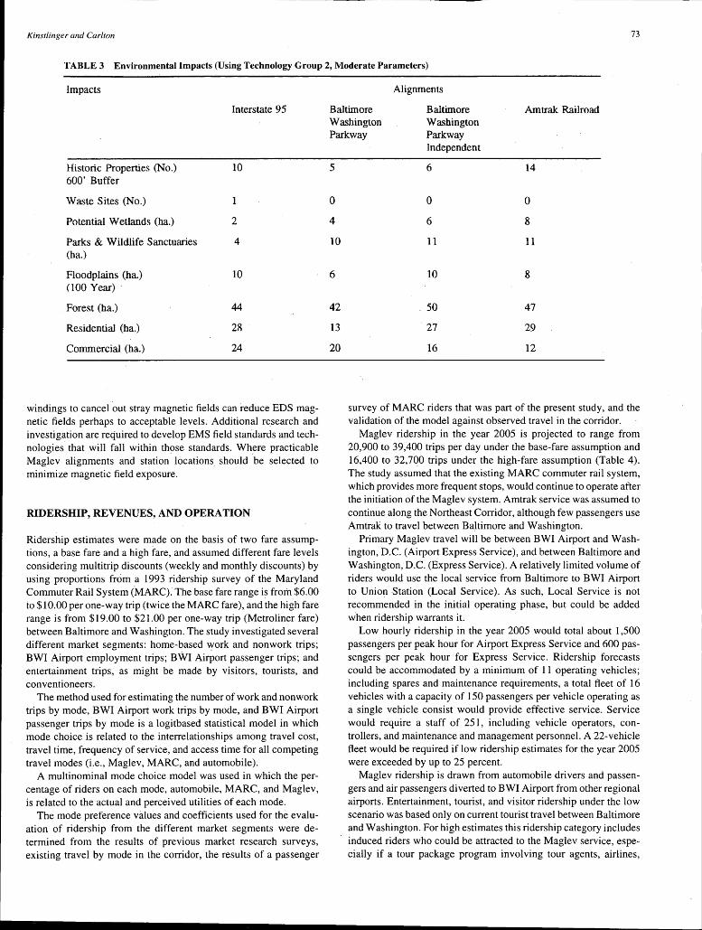
Kinstlinger and Carlton 73

TABLE3 Environmental Impacts (Using Technology Group 2, Moderate Parameters)

Impacts

Interstate 95

Historic Properties (No.) 10 600' Buffer

Waste Sites (No.)

Potential Wetlands (ha.) 2

Parks & Wildlife Sanctuaries 4 (ha.)

Floodplains (ha.) 10 (100 Year)

Forest (ha.) 44

Residential (ha.) 28

Commercial (ha.) 24

windings to cancel out stray magnetic fields can reduce EDS mag­netic fields perhaps to acceptable levels. Additional r~search and investigation are required to develop EMS field standards and tech­nologies that will fall within those standards. Where practicable Maglev alignments and station locations. should be selected to minimize magnetic field exposure.

RIDERSHIP, REVENUES, AND OPERATION

Ridership estimates were made on the basis of two fare assump­tions, a base fare and a high fare, and assumed different fare levels considering multitrip discounts (weekly and monthly discounts) by using proportions from a 1993 ridership survey of the Maryland Commuter Rail System (MARC). The base fare range is from $6.00 to $10.00 per one-way trip (twice the MARC fare), and the high fare range is from $19 .00 to $21.00 per one-way trip (Metro liner fare) between Baltimore and Washington. The study investigated several different market segments: home-based ~ork and nonwork trips; BWI Airport employment trips; BWI Airport passenger trips; and entertainment trips, as might be made by visitors, tourists, and conventioneers.

The method used for estimating the number of work and non work trips by mode, BWI Airport work trips by mode, and BWI Airport passenger trips by mode is a logitbased statistical model in which mode choice is related to the interrelationships among travel cost, travel time, frequency of service, and access time for all competing travel modes (i.e., Maglev, MARC, and automobile).

A multinominal mode choice model was used in which the per­centage of riders on each mode, automobile, MARC, and Maglev, is related to the actual and perceived utilities of each mode.

The mode preference values and coefficients used for the evalu­ation of ridership from the different market segments were de­termined from the results of previous market research surveys, existing travel by mode in the corridor, the results of a passenger

Alignments

Baltimore Baltimore Amtrak Railroad Washington Washington Parkway Parkway

5

0

4

10

6

42

13

20

Independent

6 14

0 0

6 8

11 11

10 8

50 47

27 29

16 12

survey of MARC riders that was part of the present study, and the validation of the model against observed travel in the corridor.

Maglev ridership in the year 2005 is projected to range from 20,900 to 39,400 trips per day under the base-fare assumption and 16,400 to 32,700 trips under the high-fare assumption (Table 4). The study assumed that the existing MARC commuter rail system, which provides more frequent stops, would continue to operate after the initiation of the Maglev system. Amtrak service was assumed to continue along the Northeast Corridor, although few passengers use Amtrak to travel between Baltimore and Washington.

Primary Maglev travel will be between BWI Airport and Wash­ington, D.C. (Airport Express Service), and between Baltimore and Washington, D.C. (Express Service). A relatively limited volume of riders would use the local service from Baltimore to BWI Airport to Union Station (Local Service). As such, Local Service is not recommended in the initial operating phase, but could be added when ridership warrants it.

Low hourly ridership in the year 2005 would total about 1,500 passengers per peak hour for Airport Express Service and 600 pas­sengers per peak hour for Express Service. Ridership forecasts could be accommodated by a minimum of 11 operating vehicles; including spares and maintenance requirements, a total fleet of 16 vehicles with a capacity of 150 passengers per vehicle operating as a single vehicle consist would provide effective service. Service would require a staff of 251, including vehicle operators, con­trollers, and maintenance and management personnel. A 22-vehicle fleet would be required if low ridership estimates for the year 2005 were exceeded by up to 25 percent.

Maglev ridership is drawn from automobile drivers and passen­gers and air passengers diverted to BWI Airport from other regional airports. Entertainment, tourist, and visitor ridership under the low scenario was based only on current tourist travel between Baltimore and Washington. For high estimates this ridership category includes induced riders who could be attracted to the Maglev service, espe­cially if a tour package program involving tour agents, airlines,

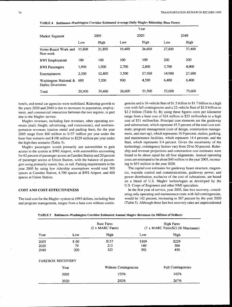
74 TRANSPORTATION RESEARCH RECORD 1489

TABLE 4 Baltimore-Washington Corridor Estimated Average Daily Maglev Ridership (Base Fares)

Market Segment 2005

·Low High

Home-Based Work and 15,800 21,800 Non-work

BWI Employment 100. 100

BWI Passengers 1,900 1,900

Entertainment 2,500 12,400

Washington National & 600 3,200 Dulles Diversions

Total 20,900 39,400

hotels, and rental car agencies were mobilized. Ridership growth to the years 2020 and 2040 is due to increases in population, employ­ment, and commercial interaction between the two regions, in part due to the Maglev service.

Maglev revenues, including fare revenues, other operating rev­enues (mail, freight, advertising, and concessions), and nontrans­portation revenues (station rental and parking fees), for the year 2005 range from $60 million to $157 million per year under the base-fare scenario and $108 million to $229 million per year under the high-fare scenario (Table 5).

Maglev passengers would primarily use automobiles to gain access to the system at BWI Airport, with automobiles accounting for 62 percent of passenger access at Camden Station and 20 percent of passenger access at Union Station, with the balance of passen­gers using primarily transit, bus, or rail. Parking requirements in the year 2005 by using low ridership assumptions would total 500 spaces at Camden Station, 4, 700 spaces at BWI Airport, and 400 spaces at Union Station.

COST AND COST-EFFECTIVENESS

The total cost for the Maglev system in 1993 dollars, including fleet and program management, ranges from a base cost without contin-

Year

2020 2040

Low High Low High

19,400 26,600 27,800 37,400

100 100 200 200

2,700 2,800 3,700 4,000

3,500 17,500 14,900 27,600

900 4,500 6,400 6,400

26,600 51,500 53,000 75,600

gencies and a 16-vehicle fleet of $1.5 billion to $1. 7 billion to a high cost with full contingencies and a 22-vehicle fleet of $2.0 billion to $2.2 billion (Table 6). By using these figures costs per kilometer range from a base cost of $24 million to $25 million/km to a high cost of $31 million/km. Principal cost elements are the guideway and substructure, which represent 45.5 percent of the total cost esti­mate; program management (cost of design, construction manage­ment, and start-up), which represents 16.9 percent; station, parking, and maintenance facilities, which represent 14.4 percent; and the fleet, which represents 9.4 percent. Given the uncertainty of the technology, contingency factors vary from 20 to 50 percent. Rider­ship and revenue projections and construction cost estimates were found to be about equal for all four alignments. Annual operating costs are estimated to be about $40 million in the year 2005, increas­ing to $53 million in the year 2020.

The capital cost estimates for guideway beam structure, magnet­ics, wayside control and communications; guideway power, and power distribution, exclusive of the cost of substations, are based on a blend of U.S. Maglev technologies as de~eloped by the U.S. Corps of Engineers and other NMI specialists. ·

In the first year of service, year 2005, fare box recovery, consid­ering only operating and maintenance costs with full contingencies, would be 142 percent, increasing to 267 percent by the year 2020 (Table 5). Although these fare box recovery rates are unprecedented

TABLE 5 Baltimore-Washington Corridor Estimated Annual Maglev Revenues (in Millions of Dollars)

Year Low

2005 $ 60 2020 79 2040 200

FAREBOX RECOVERY

Year

2005

2020

Base Fares (2 x MARC Fares)

High

$157 213 323

Without Contingencies

155%

292%

High Fares (7 x MARC Fares/$21.00 Maximum)

Low High

$109 $229 140 304 302 450

Full Contingencies

142%

267%

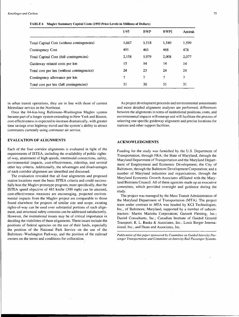
Kinstlinger and Carlton 75

TABLE 6 Maglev Summary Capital Costs (1993 Price Levels in Millions of Dollars)

Total Capital Cost (without contingencies)

Contingency Cost

Total Capital Cost (full contingencies)

Guideway related cost<; per km

Total cost per km (without contingencies)

Contingency allowance per km

Tptal cost per km (full contingencies)

in urban transit operations, they are in line with those of current Metroliner service in the Northeast.

Once the 64-km-long Baltimore-Washington Maglev system beca111e part of a longer system extending to New York and Boston, cost-effectiveness is expected to increase dramatically, with greater time savings over highway travel and the system's ability to attract commuters currently using commuter air service.

EVALUATION OF ALIGNMENTS

Each qf the four corridor alignments is evaluated in light of the requirements of IS TEA, including the availability of public rights­of-way, attainment of high speeds, intermodal connections, safety, envirorimental impacts, cost-effectiveness, ridership, and several other key criteria. Additionally, the advantages and disadvantages of each corridor alignment are identified and discussed.

The evaluation revealed that all four alignments and proposed station locations meet the basic ISTEA criteria and could success­fully host th~ Maglev prototype program, more specifically, that the ISTEA speed objective of 483 km/hr (300 mph) can be attained, cost-effectiveness measures are encouraging, projected environ­mental impacts from the Maglev project are comparable to those found elsewhere for projects of similar size and scope, existing rights-of-way can be used over substantial portions of each align­ment, and structural safety concerns can be addressed satisfactorily. However, the institutional issues may be of critical importance in deciding the viabilities of these alignments. These issues include the positions of federal agencies on the use of their lands, especially the position of the National Park Service on the use of the Baltimore-Washington Parkway, and the position of the railroad owners on the terms and conditions for collocation.

I-95 BWP BWPI Amtrak

1,667 1,518 1,540 1,599

491 461 468 478

2,158 1,979 2,008 2,077

15 14 14 14

24 23 24 24

7 7 7 7

31 30 31 31

As project development proceeds and environmental assessments and more detailed alignment analyses are performed, differences between the alignments in terms of institutional positions, costs, and environmental impacts will emerge and will facilitate the process of selecting one specific guideway alignment and precise locations for stations and other support facilities.

ACKNOWLEDGMENTS

Funding for the study was furnished by the U.S. Department of Transportation, through FRA; the State of Maryland, through the Maryland Department of Transportation and the Maryland Depart­ment of Employment and Economic Development; the City of Baltimore, through the Baltimore Development Corporation; and a number of Maryland industries and organizations, through the Maryland Economic Growth Associates affiliated with the Mary­land Business Council. All of these agencies made up an executive committee, which provided oversight and guidance during the study.

The project was managed by the Mass Transit Administration of the Maryland Department of Transportation (MT A). The project team under contract to MT A was headed by KCI Technologies, Inc., of Baltimore, Maryland, supported by a number of subcon­tractors: Martin Marietta Corporation; Gannett Fleming, Inc.; Daniel Consultants, Inc.; Canadian Institute of Guided Ground Transport; R. L. Banks & Associates, Inc.; Louis Berger Interna­tional, Inc.; and Dunn and Associates, Inc.

Publication of this paper sponsored by Committee on Guided Intercity Pas­senger Transportation and Committee on Intercity Rail Passenger Systems.