Tribological Studies on Scuffing Due to the Influence of

University of Illinois at Urbana-Champaign

Air Conditioning and Refrigeration Center A National Science Foundation/University Cooperative Research Center

Tribological Studies on Scuffing Due to the Influence of Carbon Dioxide

Used as a Refrigerant in Compressors

N. G. Demas, A. A. Polycarpou, and T. F. Conry

ACRC TR-222 December 2003

For additional information:

Air Conditioning and Refrigeration Center University of Illinois Mechanical & Industrial Engineering Dept. 1206 West Green Street Urbana, IL 61801 Prepared as part of ACRC Project #133 Tribological Studies on Scuffing Due to the Influence of CO2 Used as a Refrigerant in Compressors (217) 333-3115 A. A. Polycarpou and T. F. Conry, Principal Investigators

The Air Conditioning and Refrigeration Center was founded in 1988 with a grant from the estate of Richard W. Kritzer, the founder of Peerless of America Inc. A State of Illinois Technology Challenge Grant helped build the laboratory facilities. The ACRC receives continuing support from the Richard W. Kritzer Endowment and the National Science Foundation. The following organizations have also become sponsors of the Center. Alcan Aluminum Corporation Amana Refrigeration, Inc. Arçelik A. S. Behr GmbH and Co. Carrier Corporation Copeland Corporation Daikin Industries, Ltd. Delphi Harrison Thermal Systems Embraco S. A. General Motors Corporation Hill PHOENIX Honeywell, Inc. Hydro Aluminum Adrian, Inc. Ingersoll-Rand Company Lennox International, Inc. LG Electronics, Inc. Modine Manufacturing Co. Parker Hannifin Corporation Peerless of America, Inc. Samsung Electronics Co., Ltd. Sanyo Electric Co., Ltd. Tecumseh Products Company Trane Visteon Automotive Systems Wieland-Werke, AG Wolverine Tube, Inc. For additional information: Air Conditioning & Refrigeration Center Mechanical & Industrial Engineering Dept. University of Illinois 1206 West Green Street Urbana, IL 61801 217 333 3115

iii

Abstract

The refrigeration and air conditioning industry has expressed a great interest in the use of carbon dioxide

(CO2) as a refrigerant. CO2 is anticipated to replace HFC refrigerants, which are known to have a negative effect on

the environment. The reason behind the interest in CO2 is the fact that it is a natural refrigerant, thus

environmentally acceptable. Of course, such a replacement raises concerns regarding design criteria and

performance due to the different thermodynamic properties of CO2 and the very different range of pressures required

for the CO2 refrigeration cycle.

So far, work related to CO2 has been done from a thermodynamics point of view and researchers have

made significant progress developing automotive and portable air-conditioning systems that use the environmentally

friendly carbon dioxide as a refrigerant. The purpose of this work is to develop an understanding of how CO2 plays

a role from a tribology standpoint. More specifically, the goal of this work is to gain an understanding on how CO2

influences friction, lubrication, wear and scuffing of tribological pairs used in compressors.

Work in the area of tribology related to CO2 is very limited. Preliminary work by Cusano and coworkers

showed that consistent data for tests using CO2 could not be acquired nor could a satisfactory explanation be offered

for the inconsistency. Their results triggered the initiation of the work presented here. In this first attempt to

understand the tribological behavior of CO2 several problems were encountered. During this work we noted that its

behavior, unlike conventional refrigerants, could not always be predicted. We believe that this can be attributed to

the thermodynamic properties of CO2, which cannot be ignored when studying its tribological behavior.

Thermodynamic Properties such as miscibility are very important when tribological testing is performed. A limiting

factor with our tester was that it was not designed for CO2 testing, but for other conventional refrigerants and

therefore made previously developed testing protocols non-applicable with CO2. Through a different approach and

some modifications to our tester we were able to establish a protocol for testing under the presence of CO2. CO2

was then compared to R134a and the experimental results showed that it performs equally well.

iv

Table of Contents

Page

Abstract ......................................................................................................................... iii

List of Figures............................................................................................................... vi

List of Tables .............................................................................................................. viii

Chapter 1. Carbon Dioxide (CO2) .................................................................................1 1.1 Tribology of CO2 Compressors .....................................................................................................1 1.2 General Background Related to CO2 ............................................................................................1 1.3 CO2 Phase Diagram ........................................................................................................................2

1.3.1 Triple Point.............................................................................................................................................2 1.3.2 Critical Point...........................................................................................................................................2 1.3.3 CO2 as a Liquid ......................................................................................................................................3 1.3.4 CO2 as a Solid.........................................................................................................................................3

1.4 CO2 Used as Refrigerant ................................................................................................................3 1.5 Miscibility of Lubricants in CO2 .....................................................................................................5 1.6 Thesis Outline .................................................................................................................................6

Chapter 2. High Pressure Tribometer (HPT) and Experimental Tribological Testing............................................................................................................................7

2.1 Introduction .....................................................................................................................................7 2.2 Contact Geometry.........................................................................................................................10 2.3 Instrumentation .............................................................................................................................11

2.3.1 Load vs. Time.......................................................................................................................................13 2.3.2 Friction Coefficient vs. Time................................................................................................................13 2.3.3 Temperature vs. Time...........................................................................................................................13 2.3.4 Electrical Contact Resistance (ECR) vs. Time .....................................................................................13

2.4 Experimental Procedure and Conditions ...................................................................................15 2.5 Experimental Setups.....................................................................................................................16

2.5.1 Preliminary Type I, II and III Experiments ..........................................................................................16 2.5.2 Type I – Dry, Non-Lubricated under Presence of Refrigerant .............................................................17 2.5.3 Type II- Lubricated Using Spray of Refrigerant ..................................................................................18 2.5.4 Type III-Lubricated Using Spray of Lubricant and Refrigerant ...........................................................19 2.5.5 Type IV-Fully Submerged in PAG Lubricant ......................................................................................19 2.5.6 CO2/Lubricant Re-circulation Supply Setup.........................................................................................20 2.5.7 Type V-Direct Application of PAG Lubricant via Absorbing Medium ...............................................22

Chapter 3. Results and Discussion............................................................................24 3.1 Introduction ...................................................................................................................................24 3.2 Preliminary Experiments-Main findings .....................................................................................24

3.2.1 Cusano-Stokes Experiments (1999) .....................................................................................................24 3.2.2 Poziemski-Reifman Experiments (Summer 2001) ...............................................................................25

v

3.3 Type I-Dry, Non-Lubricated under Presence of Refrigerant .....................................................27 3.3.1 Effects of Temperature and Pressure....................................................................................................27 3.3.2 Comparison of CO2 with R134a and air ...............................................................................................32

3.4 Type IV-Fully Submerged in PAG Lubricant ..............................................................................35 3.5 Type V-Direct Application of PAG Lubricant via Absorbing Medium......................................38

3.5.1 Comparison of CO2 with R134a...........................................................................................................38 Chapter 4. Experimental Uncertainties and Techniques..........................................41

4.1 Experimental Techniques ............................................................................................................41 4.1.1 Load Selection for Type I-Dry, Non-Lubricated Tests.........................................................................41 4.1.2 Load Selection for Type V-Direct Application of PAG Lubricant.......................................................42

4.2 Pin Separation (HPT Low Load Capability) ................................................................................42 4.3 Examples of Erratic Behavior due to Software Issue................................................................43 4.4 Avoiding Condensation................................................................................................................44 4.5 Repeatability of Results ...............................................................................................................44

Chapter 5. Conclusions and Recommendations ......................................................46 5.1 Main Conclusions .........................................................................................................................46 5.2 Future Work ...................................................................................................................................46

Bibliography.................................................................................................................47

Appendix A...................................................................................................................48

vi

List of Figures

Page

Figure 1.1 - Phase Diagram for CO2 ..............................................................................................................................2 Figure 1.2 - CO2/R134a/R22 Comparison of Pressure Levels.......................................................................................4 Figure 1.3 - Typical Transcritical CO2 Cycle for Refrigeration ....................................................................................4 Figure 1.4 - Typical operating conditions for CO2 and R134a.......................................................................................5 Figure 1.5 - Miscibility Chart of Different Lubricants in CO2 (Seeton, 2000) ..............................................................6 Figure 2.1 - The High Pressure Tribometer ...................................................................................................................7 Figure 2.2 - Schematic of HPT Pressure Chamber and Lubricant Supply System ........................................................8 Figure 2.3 - The Four Main Sub-systems of the Tribometer .........................................................................................9 Figure 2.4 - Geometries of Contact (a) Pin-on-Disc, (b) Shoe-on-Disk ......................................................................10 Figure 2.5 - Setup for Spraying Nozzle and Specimen Holder....................................................................................11 Figure 2.6 - Typical Endurance Experiment................................................................................................................12 Figure 2.7 - Typical Scuffing Experiment ...................................................................................................................12 Figure 2.8 - Schematic of Electrical Contact Resistance Measuring Circuit ...............................................................14 Figure 2.9 – Typical Samples (a) Disk, (b) Pin and Shoe............................................................................................15 Figure 2.10 - Base Fixture ...........................................................................................................................................17 Figure 2.11 - Tribometer Chamber ..............................................................................................................................17 Figure 2.12 - Heating of the Pressure Vessel...............................................................................................................18 Figure 2.13 - Experimental Setup for CO2/Lubricant Supply System .........................................................................20 Figure 2.14 - Filters Used in the Re-circulation Setup (a) PEEK (b) Stainless Steel...................................................21 Figure 2.15 - Modified Fixture for New Lubricant/CO2 Supply System.....................................................................21 Figure 2.16 - Setup for Direct Application of Lubricant via Absorbing Medium .......................................................22 Figure 3.1 - Scuffing Pressure-Velocity Diagram for Al 390-T6 and 52100 Steel in R134a/PAG or CO2/PAG ........25 Figure 3.2 - Scuffing Pressure-Velocity Diagram for Al 390-T6 and 52100 Steel in CO2/POE .................................26 Figure 3.3 - CO2, 50 psi, 0°C.......................................................................................................................................28 Figure 3.4 - CO2, 50 psi, 60°C.....................................................................................................................................28 Figure 3.5 - CO2, 50 psi, 120°C...................................................................................................................................29 Figure 3.6 - CO2, 200 psi, 0°C.....................................................................................................................................30 Figure 3.7 - CO2, 200 psi, 60°C...................................................................................................................................30 Figure 3.8 - CO2, 200 psi, 120°C.................................................................................................................................31 Figure 3.9 - Friction Coefficients for Constant Load Tests for CO2 at Different Operating Conditions .....................31 Figure 3.10 - Contact Temperatures for Constant Load Tests for CO2 at Different Operating Conditions .................32 Figure 3.11 - CO2, 50 psi, 60°C...................................................................................................................................33 Figure 3.12 - R134a, 25 psi, 60°C ...............................................................................................................................33 Figure 3.13 - Air, 60°C ................................................................................................................................................34 Figure 3.14 - Wear Measurement for CO2, R134a and air, 50 psi, 60°C.....................................................................35 Figure 3.15 – Submerged Test in PAG lubricant in a CO2 Environment for a Time Duration of 10 minutes.............36 Figure 3.16 – Submerged Test in PAG lubricant in a CO2 Environment for a Time Duration of 20 minutes.............36 Figure 3.17 - Submerged Test in PAG Lubricant in a CO2 Environment for a Time Duration of 22 minutes ............37

vii

Figure 3.18 - Submerged Test in PAG Lubricant in a CO2 Environment for a Time Duration of 25 minutes ............37 Figure 3.19 - Microscope Image of Al390-T6 Disk: Sample C (t = 22 min)...............................................................38 Figure 3.20 - CO2, 200 psi, 120°C...............................................................................................................................39 Figure 3.21 - R134a, 25 psi, 120°C .............................................................................................................................39 Figure 3.22 - Wear Measurement for CO2 (200 psi, 120°C) and R134a (25 psi, 120°C) ............................................40 Figure 4.1 - Failure due to Increase in Load under Dry Conditions ............................................................................42 Figure 4.2 - Pin Separation as a Result of Low Load ..................................................................................................43 Figure 4.3 - Failure due to a Non-functioning Data Acquisition Board ......................................................................44 Figure A.1 - Temperature-Entropy Diagram for CO2 ..................................................................................................48 Figure A.2 - Temperature-Entropy Diagram for R134a ..............................................................................................48 Figure A.3 - Temperature-Entropy Diagram for R410a ..............................................................................................49

viii

List of Tables

Page

Table 1.1 - Characteristics of CO2 (Lorentzen, 1995) ...................................................................................................3 Table 3.1 experimental conditions and results obtained for CO2, R134a and air ........................................................35 Table A.1 - Properties of Carbon Dioxide (ASHRAE, 1969)......................................................................................49 Table A.2 - Properties of R12 (ASHRAE, 1969) ........................................................................................................50 Table A.3 - Composition Information for PARCO LUBRITE 2...............................................................................50

1

Chapter 1. Carbon Dioxide (CO2)

1.1 Tribology of CO2 Compressors Work in the area of tribology related to CO2 is very limited. Most of the work related to CO2 has focused

on the development of the main components for the required transcritical CO2 cycle such as the compressor and the

expansion device but always with a focus on the thermodynamic aspect. Most of this development is at a prototype

stage design and includes scroll compressors (Hagita et al., 2002), hermetic compressors (Suss, 2000), hermetic

swing compressors (Ohkawa, 2002), and piston-cylinder expansion devices (Baek et al., 2002). Researchers have

also focused on the aspect of lubrication in refrigeration compressors using CO2 (Johnson, 1998). Some aspects of

their work are related to tribology in the sense that they involve studies on lubrication of bearings in a scroll

compressor. However, material examination of surfaces in compressors that use CO2, comparative studies on

friction, wear, lubrication, scuffing or on the effects of the environmental conditions using different refrigerants is

absent from the open literature as of this date.

Preliminary work by Cusano and Stokes (1999) showed that testing with CO2 can be an intricate task.

Their preliminary results showed large variability in the scuffing load that could not be adequately explained. Such

task, dealing with a comparative study of refrigerants and their tribological performance, has not been undertaken

before which makes the work of tribology related to CO2 a building block of significant importance.

1.2 General Background Related to CO2 Carbon dioxide (CO2) was first recognized by Jan Baptista van Helmont (1580-1644) who detected it in the

products of both fermentation and charcoal burning. It occurs in the products of combustion of all carbonaceous

fuels and can be recovered from them in a variety of ways. It is present in the atmosphere in small quantities being

uniformly distributed over the earth's surface at a concentration of about 0.033% or 330 parts per million. Because

the concentration of CO2 in the atmosphere is very low, it is not practical to obtain the gas by extracting it from air.

Most commercial CO2 is recovered as a by-product of other processes, such as the production of ethanol by

fermentation and the manufacture of ammonia, from flue gases by absorption processes, and furnace operations.

Some CO2 is obtained from the combustion of coke or other carbon-containing fuels. CO2 is also a product of

animal metabolism and is important in the life cycles of both animals and plants. It finds uses in solid, liquid and

gaseous form in a variety of industrial applications such as welding, beverage carbonation and in fire extinguishers.

CO2 dissolves readily in many liquids. Under normal temperature and pressure conditions, CO2 gas

dissolves in an equal volume of water. The greater the pressure, the more CO2 a liquid can hold in solution, but

excess CO2 remains dissolved only as pressure is applied. When released, excess CO2 escapes in the effervescent

bubbling characteristics of uncapped soft drinks. CO2 is not very reactive at normal temperatures. It does however

form carbonic acid (H2CO3) in aqueous solutions, which is a weak and unstable acid that tends to revert to CO2 and

H2O. H2CO3 undergoes the typical reactions of a weak acid to form salts and esters. CO2 is very stable at normal

temperatures, but forms CO and O2 when heated above 1700°C.

CO2 can be reduced by several methods, the most common being its reaction with hydrogen. It can also be

reduced with hydrocarbons and carbon at elevated temperatures. CO2 will react with ammonia to form ammonium

carbonate, which is used as the first stage of urea manufacture. CO2 is a normal constituent of exhaled air but high

2

concentrations of the gas are hazardous. Five percent of CO2 by volume in air increases the breathing rate and

prolonged exposure to volumes greater than 5% can cause unconsciousness and/or death. Since carbon dioxide is

almost 53% heavier than air with a specific gravity of 1.53 at 21°C, it will settle to the bottom of a room or container

and displace air. In addition to being a component of the atmosphere, CO2 also dissolves in the water of the oceans.

The most important properties of carbon dioxide have been summarized in Table A.1 (ASHRAE, 1969) in the

Appendix.

1.3 CO2 Phase Diagram CO2 can exist in three states: gas, liquid and solid. At normal temperatures and pressures, CO2 is a colorless

gas. When compressed and cooled to the proper temperature, the gas turns into a liquid. The liquid in turn can be

converted into solid known as dry ice. The dry ice, on absorbing heat, returns to its natural gaseous state. There are

two interesting points one can observe on the phase diagram of CO2: the triple point and the critical point.

1.3.1 Triple Point The triple point is the point where CO2 can exist simultaneously in its three states as gas, liquid and solid.

The pressure and temperature that correspond to the triple point are 75.35 psi and -56.6°C (-69.88°F), respectively.

If the pressure is reduced from the triple point, the liquid flashes to solid and gas. If the temperature is reduced, the

liquid freezes. If the temperature is increased, the liquid boils, which generates gas. These phase changes can be

seen in Figure 1.1.

1.3.2 Critical Point Above the critical temperature point of 31.04°C (87.87°F) it is impossible to liquefy the gas by increasing

the pressure above the corresponding critical pressure of 1069.96 psi. This is evident in Figure 1.1 since the liquid-

gas line stops right at the critical point. At temperatures higher than this point there can no longer be two phases.

There is only a single phase, which is a very dense gas often called a supercritical fluid.

0.15

1.5

15

150

1500

15k

Pres

sure

(psi

)

Temperature (oC)

-40-120 -100 -80 -60 -20 0 20 40 60 80

CO2 Liquid

Triple Point:-56.6oC, 75.35 psi

CO2 Solid

Critical Point:31.04oC, 1069.96 psi

Solid+

Gas

Liquid+Gas

Solid+Liquid

CO2 Gas

0.15

1.5

15

150

1500

15k

Pres

sure

(psi

)

Temperature (oC)

-40-120 -100 -80 -60 -20 0 20 40 60 80

CO2 Liquid

Triple Point:-56.6oC, 75.35 psi

CO2 Solid

Critical Point:31.04oC, 1069.96 psi

Solid+

Gas

Liquid+Gas

Solid+Liquid

CO2 Gas

Figure 1.1 - Phase Diagram for CO2

3

1.3.3 CO2 as a Liquid CO2 is most commonly stored and transported as a liquid. CO2 does not exist in liquid form at atmospheric

pressure at any temperature. The pressure-temperature phase diagram of Figure 1.1 shows that liquid CO2 at 21°C

(70°F) requires a pressure of 441 psi. The lowest pressure at which liquid CO2 exists is at the triple point at 75.35

psi and that is the minimum pressure required in order to remain a liquid.

1.3.4 CO2 as a Solid The normal temperature of solid CO2 (dry ice) is -78.45°C (-109.21°F). At ambient temperature and

atmospheric pressure, the solid sublimes slowly, leaving no residue, as it changes directly back to gaseous form.

1.4 CO2 Used as Refrigerant In recent years, the refrigeration industry has shown a great deal of interest in the use of CO2 as a

refrigerant with the potential to replace commonly used refrigerants. CO2 is a proven viable refrigerant. It has been

used in the past as a refrigerant, but the high pressures at which CO2 systems have to be operated at and the low

critical temperature limited its use in refrigeration systems. However, recent advances in compressor designs and

prototype systems have demonstrated significant improvements in energy efficiency compared to R134a (Pettersen,

1997).

For nearly six decades, chlorofluorocarbon refrigerants (CFCs) have been used for as solvents, aerosol

propellants and refrigerants. CFCs are long-lived compounds which, when released, rise to the stratosphere where

they are decomposed by UV light and form free chlorine. The chlorine released reacts with the earth’s ozone.

Chlorine atoms in the stratosphere are very reactive and each one may destroy hundreds of thousands of molecules

of ozone before removed. Their harmful effect on the Earth's protective ozone layer was first published by Rowland

and Molina in 1974. Subsequently, the ozone hole over the Antarctic was discovered and heightened world

attention that led to the Montreal Protocol of 1989. Over the same period, it was discovered that CFCs also

contributed significantly to the world's greenhouse warming problem. The global warming potential (GWP) of the

CFC refrigerant R12 is 7100 times that of carbon dioxide over twenty years (Lorentzen, 1995). The GWP

represents how much a given mass of a chemical contributes to global warming over a given time period compared

to the same mass of carbon dioxide whose GWP is defined as 1.0. The response of the chemical industry was to

develop new synthetic refrigerants without the harmful chlorine atoms, which cause ozone depletion. These are

known as hydrofluorocarbons (HFCs), of which the best known is R134a. However, their high global warming

potential is also significant, though less than that of CFCs as it can be seen in Table 1.1.

Carbon dioxide on the other hand, has no ozone depleting potential and a negligible direct global warning

effect as seen on Table 1.1.

Table 1.1 - Characteristics of CO2 (Lorentzen, 1995)

Ozone Depleting Potential

Global Warming Potential (20 years integration time)

Critical Temperature (°C)

CO2 0 1 31.1 R134a 0 3100 101.2

R22 0.05 4100 96.1 R12 1.0 7100 112.0

4

CO2 is non-flammable, chemically inactive, nontoxic and inexpensive. Due to these properties, along with

the fact that it is a natural refrigerant and therefore environmentally acceptable, the refrigeration and air conditioning

industry has expressed a great interest in its use and is anticipated to replace HFC refrigerants. However, such a

replacement raises concerns regarding design criteria and performance and safety due to the different

thermodynamic properties of CO2 and the very different range of pressures required for the CO2 refrigeration cycle

for typical applications in refrigeration. The difference in the range of pressures between CO2, R134a and R22 can

be seen in Figure 1.2.

0

200

400

600

800

1000

1200

-40 -20 0 20 40 60

Temperature (oC)

Pre

ssur

e (p

si)

CO2

R22

R134a

Figure 1.2 - CO2/R134a/R22 Comparison of Pressure Levels

A typical transcritical cycle for CO2 is shown in Figure 1.3. Unlike R134a, the CO2 gas is compressed well

above the critical point and the heat rejection process takes place in the critical region.

1160psi

435psi

0

50

100

150

250

200

-50

-100-0.3-0.5 0.0 0.3 0.5 0.8 1.0 1.3 1.5 1.8

Entropy (KJ/Kg-K)

Tem

pera

ture

(o C)

Gas Cooler

Expansion

EvaporatorCompression

2000psi1450psi

1160psi

435psi

0

50

100

150

250

200

-50

-100-0.3-0.5 0.0 0.3 0.5 0.8 1.0 1.3 1.5 1.8

Entropy (KJ/Kg-K)

Tem

pera

ture

(o C)

Gas Cooler

Expansion

EvaporatorCompression

2000psi1450psi

Figure 1.3 - Typical Transcritical CO2 Cycle for Refrigeration

Typical operating conditions for CO2 and R134a are shown in Figure 1.4. Both are plotted on the same

graph for contrast. The discharge pressure with CO2 is extremely high and the critical temperature at 31°C (1070

psi) is very low. For single stage systems this requires transcritical-operating conditions with discharge pressures

5

greater than 1500 psi. Also, the pressure of CO2 is about 10 times that of R134a, so when designing CO2

compressors it is vital to solve the problems that arise by the need for higher loads of the sliding parts and the

differential pressures of the sealing parts (Hagita et al., 2002). Another major problem with CO2 is that its

thermodynamic cycle characteristics result in system coefficients of performance (COP) that are typically lower than

HFC vapor compression systems (Brown et al., 2002).

600

900

1200

1500

2100

1800

300

0150100 200 250 300 350 400 450 500 550

Enthalpy(KJ/Kg)

Pres

sure

(psi

)

CO2R134a Gas Cooler

Evaporator

Expansion Compression

600

900

1200

1500

2100

1800

300

0150100 200 250 300 350 400 450 500 550

Enthalpy(KJ/Kg)

Pres

sure

(psi

)

CO2R134a Gas Cooler

Evaporator

Expansion Compression

Figure 1.4 - Typical operating conditions for CO2 and R134a

So, at a glance it may seem that CO2 is in some ways inferior to other refrigerants. However, due to its

high volumetric capacity and the elimination of recovery and recycling equipment and the subsequent procedures,

carbon dioxide has received much attention for several applications.

1.5 Miscibility of Lubricants in CO2 The role of lubricants in refrigeration compressors is to reduce friction and prevent wear. Lubricant

chemistry, density, miscibility and solubility with CO2 are some very important parameters one would have to take

into consideration. A wide range of optimized lubricants is available for different refrigerants. Lubricant options

allow the selection of particular performance characteristics appropriate to the system. Therefore, the selection of a

lubricant for a CO2 compressor is of great importance since it can have a major impact on the performance and

reliability of the system. It has been suggested that lubrication of CO2 compressors is difficult due to the high

operating pressure of CO2. Solubility is also of particular interest, however, the major concern is miscibility of

different lubricants in CO2. A refrigerant and lubricant are described as miscible when they form one single liquid

phase. On the other hand solubility can be thought of as when the refrigerant contains a proportion of the lubricant

and vice-versa. An immiscible mixture of lubricant and refrigerant can still possess a degree of mutual solubility.

Modern synthetic lubricants can be designed to interact with refrigerants in specific ways. The most commonly

used lubricants with CO2 as far as experience or compatibility is concerned are polyol ester (POE), and polyalkylene

glycol (PAG) lubricants. In Figure 1.5 we can see a miscibility chart (Seeton, 2000) with these lubricants.

6

Immiscible

POE Miscible

MisciblePAO

PAG

M

AB

POE

30

20

10

0

-10

-20

-30

-40

Wt % Lubricant in CO2

0 10 20 30 40 50 60 70 80 90 100

Tem

pera

ture

(o C)

Immiscible

POE Miscible

MisciblePAO

PAG

M

AB

POE

30

20

10

0

-10

-20

-30

-40

Wt % Lubricant in CO2

0 10 20 30 40 50 60 70 80 90 100

Tem

pera

ture

(o C)

Figure 1.5 - Miscibility Chart of Different Lubricants in CO2 (Seeton, 2000)

POEs have wide market acceptance with HFC refrigerants. Applications include appliance, refrigeration

and air-conditioning. Ester chemistry allows the use of numerous alcohols and acids that can be combined to make

esters with desired properties (Randles, 1999). As a result, POE-based refrigeration lubricants with structures

designed to control miscibility and solubility and other properties have been developed. POEs have a high degree of

solubility and miscibility with CO2.

PAGs are polymers of alkylene glycols. Typically, they are polymers of ethylene oxide, propylene oxide,

butylenes oxide or copolymers of the above. The chemical structure of PAGs can also be varied to give desired

miscibility and solubility with the HFC refrigerants. This is often achieved by varying the ratios of ethylene oxide

and propylene oxide in the synthesis process (Matlock et al., 1999). Currently, PAG is the lubricant of choice in

most R-134a automobile A/C systems. In addition, they are good candidates for use in CO2 systems.

1.6 Thesis Outline In Chapter 2, the High Pressure Tribometer (HPT) used for the experimental tribological testing, and the

experimental setups for all the different types of tests performed in this work have been described. In Chapter 3, the

motivation for performing the different types of tests has been presented along with the results and discussion of our

tests. The main point of this chapter is the fact that a test protocol for testing under refrigerant environments was

established that led to different series of tests that make comparative studies possible and allow us to obtain

qualitative results about the behavior and performance of CO2 under numerous operating conditions. Chapter 4

contains experimental techniques and uncertainties about some of the types of tests that were performed. Due to

some inconsistencies in sample preparation some of the results did not exhibit repeatability. We offer some

criticism as well as an explanation to why we believe we have presented representative results from the series of

tests that were not repeatable. Finally in Chapter 5 some conclusions and recommendations have been presented.

Under the presence of PAG lubricant and the same environmental conditions, CO2 and R134a performed almost

identically. Furthermore, in the absence of lubricant, CO2 performed very similar to R134a.

7

Chapter 2. High Pressure Tribometer (HPT) and Experimental Tribological Testing

2.1 Introduction The High Pressure Tribometer (HPT) is an instrument used to run wear and friction tests using a lower

stationary sample in contact with an upper rotating sample. It accurately simulates the environmental conditions

found in a typical air conditioning compressor. A photograph of the HPT and a schematic of its pressure chamber

are shown in Figures 2.1 and 2.2, respectively.

Figure 2.1 - The High Pressure Tribometer

8

Figure 2.2 - Schematic of HPT Pressure Chamber and Lubricant Supply System

The HPT is capable of motion in two directions. The vertical or z-axis direction is used to access the

samples, seal the high-pressure chamber, and provide the loading on the test specimens. The rotary or theta-axis

direction controls the rotary motion of the upper sample. These displacements can be controlled manually via a

control panel or through a computer. The lower stationary sample is mounted on a transducer module that measures

the forces in the three orthogonal directions (Fx, Fy, Fz) and also the moment about the z-axis (Mz). The force Fz is

in the normal or z-direction and the forces Fx, Fy are perpendicular to the z-axis. The resultant of Fx and Fy is called

Fr, and is the friction force for generalized single point sliding. This positive value divided by the normal force Fz,

provides the coefficient of friction (AMTI, 1991).

The test chamber is contained in a special pressure/vacuum housing capable of testing from 0.2 torr to 250

psi. Using a combination of heating and cooling systems, chamber temperatures from -12°C to 121°C can be

attained. The desired temperature of the rotary contact specimen is obtained by pumping heat transfer fluid through

the spindle. The temperature of the fluid is controlled by an external unit, which is capable of maintaining constant

temperatures on the spindle from 30°C to 130°C. The chamber heaters consist of one 400-Watt cartridge heater in

the upper chamber and two 400-watt cartridge heaters in the lower chamber. A lead screw that is driven by a DC

servomotor through a harmonic drive supplies the normal contact load and unidirectional rotation. The specimen

9

mounting system has been designed to be general and consists of flat lower and upper surfaces with threaded holes

to accept any specimens or fixtures for specimens. During an actual test, the lower sample is brought into contact

with the upper sample using the motor driven lead screw located at the bottom of the unit. The maximum

recommended load for this machine is 1000 lbf, in addition to the maximum chamber pressure of 250 psi, which

corresponds to a 7000 lb force that is needed to keep the chamber closed. The maximum unidirectional rotation is

2000 rpm. The HPT is equipped with computer control of the axial load and the angular velocity of the spindle.

The computer control is achieved through control boards and a set of solid-state relays. The data acquisition card

the computer uses is manufactured by National Instruments and its model number is AT-MIO-16F-5. This card has

been discontinued since 1995. It was used since 1991 but was replaced in 2003 with a demo DAQ board that we

obtained from National Instruments. The corresponding software allows for complicated loading and sliding

velocity histories.

Figure 2.3 schematically depicts the four main subsystems that make up the tribometer. The first is the

mechanical portion, which was described earlier and that contains the pressure chamber, sample holders, load

sensors, position locators, temperature cartridge heaters for the upper and lower pressure chamber and the two drive

motors that provide the vertical and rotary motion. The second section is the power box. This system contains the

power amplifiers, power distribution system, fuses and relays. The chiller is used to maintain non-test portions of

the tribometer at 20°C, which is achieved by re-circulation of heat transfer fluid in a closed loop. The last section is

the control box, which contains the motor controls, amplifiers for load measurements, temperature controls and the

microprocessor.

SENSORS

- LOAD

- TEMPERATURE

HEATERS

SAMPLE HOLDERS

MOTORS (2)

TRIBOMETER MECHANICAL CONTROL BOX

POWER BOX

RECIRCULATORHEATING/COOLING

MOTHER BOA RD

(MICROPROCESSOR)

AMPLIFIERS

MOTOR CONTROL

CARDS

TEMPERATURE CARD

PANEL CONTROLS

DC POW ER

CONTROL WIRING

SENSORS/CONTROL

SENSORS

POW ER

POWER

POW ER WIRING

MOTOR POW ER SUPPLIES

DC POW ER SUPPLIES

MISC.- FUSE, RELA YS

CHILLER

SENSORS

- LOAD

- TEMPERATURE

HEATERS

SAMPLE HOLDERS

MOTORS (2)

TRIBOMETER MECHANICAL CONTROL BOX

POWER BOX

RECIRCULATORHEATING/COOLING

MOTHER BOA RD

(MICROPROCESSOR)

AMPLIFIERS

MOTOR CONTROL

CARDS

TEMPERATURE CARD

PANEL CONTROLS

DC POW ER

CONTROL WIRING

SENSORS/CONTROL

SENSORS

POW ER

POWER

POW ER WIRING

MOTOR POW ER SUPPLIES

DC POW ER SUPPLIES

MISC.- FUSE, RELA YS

CHILLER

Figure 2.3 - The Four Main Sub-systems of the Tribometer

10

2.2 Contact Geometry In this study, we use the pin-on-disc and the shoe-on-disk contact for the experimentation as shown in

Figure 2.4. In this type of geometry thermal expansion of the specimen and other parts of the test rig do not increase

any loading on the specimen (Yoon, 1999). In addition, the apparent area of contact does not change with time due

to wear. Another advantage of this system is the fact that the rotating disc is the upper specimen, most of the wear

debris falls at the base of the pins and the effect of debris accumulation from the experiment is eliminated.

Gray Cast IronDisc (Rotating)

Ø 6.35 mm Pin(Stationary)

Miniature Thermocouple

Contact Resistance Measurement

Spindle

Gray Cast IronDisc (Rotating)

Ø 6.35 mm Pin(Stationary)

Miniature Thermocouple


Spindle

(a)

52100 Steel Shoe(Stationary)


390 Al Disk(Rotating)

Spindle

52100 Steel Shoe(Stationary)


390 Al Disk(Rotating)

Spindle

(b)

Figure 2.4 - Geometries of Contact (a) Pin-on-Disc, (b) Shoe-on-Disk

A photograph of the setup of the pin (or shoe) holder is shown in Figure 2.5. The base fixture consists of

three pieces: the main base, an outer ring, and an O-ring (Buta-N) that serves as a seal in order to accommodate tests

submerged in lubricant. When the pin-on-disk geometry is used, a miniature thermocouple can be inserted below

the sliding surfaces to provide subsurface temperature measurements during testing as shown in Figure 2.4 (b). The

11

pins are inserted into a hole in the shoe, which, in turn, is supported in a socket as shown in Figure 2.5. An

important point in this holder that should be noted is that the pin holder is self-aligning so that motion during contact

is not restricted.

The specimen holder is electrically isolated by using a non-conductive material (Formica®) so that

electrical contact resistance measurements can be provided, as it will be described below. Finally, depending on the

type of test we can have a spraying nozzle or just a plug attached to the fixture. A small hole underneath the base

fixture allows refrigerant or a mixture of refrigerant/lubricant to flow through and be sprayed near the contact area.

Thermocouple


Nozzle Base Fixture

Specimen Holder

Thermocouple


Nozzle Base Fixture

Specimen Holder

Thermocouple


Nozzle Base Fixture

Specimen Holder

Figure 2.5 - Setup for Spraying Nozzle and Specimen Holder

2.3 Instrumentation The instrumentation of the HPT includes a real-time output for the axial and friction forces, frictional

torque, and the environmental temperature. The HPT is used to conduct scuffing experiments or simply run wear

tests. In general, there are two ways that scuffing tests can be conducted in the HPT. One way is an endurance test,

from which the time to failure is obtained for given constant load and velocity conditions. The other way is a step-

loading test, for which the load is progressively increased stepwise for a specified sliding velocity until failure

occurs. Figure 2.6 shows a typical endurance test, while Figure 2.7 shows a typical step-loading test. An endurance

test corresponding to short time durations so that scuffing is avoided serves as a wear test for which the coefficient

of friction can be obtained and wear can then be quantified by means of profilometry.

Scuffing can have various manifestations. The first obvious signs of scuffing are the increased audible

noise and vibration. In a controlled laboratory environment, scuffing can be detected by sharp transitions in friction,

contact resistance and near-contact temperature.

12

0 2.5 5 7.5 10 12.5 1505

101520

Load

(lbf)

0 2.5 5 7.5 10 12.5 150

1

2

3

µ r

0 2.5 5 7.5 10 12.5 150

100200300400

Tem

pera

ture

(o C)

0 2.5 5 7.5 10 12.5 1510

-4

100

104

EC

R(O

hms)

Time (min)

Figure 2.6 - Typical Endurance Experiment

0 2 4 6 8 10 12 14 160

50

100

150

Load

(lb

f)

0 2 4 6 8 10 12 14 160

0.2

0.4

µ r

0 2 4 6 8 10 12 14 160

100200300400

Tem

pera

ture

(o C)

0 2 4 6 8 10 12 14 1610

-210

-110

010

110

2

EC

R(O

hms)

Time (min)

Figure 2.7 - Typical Scuffing Experiment

The electrical contact resistance (ECR) between the test specimens provides indirect information about the

regime of lubrication, the formation of protective surface films and the extent of metal-to-metal contact. A

schematic of the ECR measuring circuit is given in Figure 2.8. The measurement range of the circuit used is 10-6 –

10+4 Ω. This sensitivity was achieved by the development of a special four-terminal measurement circuit, methods

for noise suppression and data processing software (Sheiretov, 1997). A large drop in the ECR is an indicator for

scuffing. So the ECR is an important tribological quantity.

13

The surface temperature is also a very important tribological quantity. Its direct measurement in sliding

interfaces is somewhat difficult. Due to experimental difficulties, the temperature in the vicinity of the sliding

interface is often estimated with the aid of thermal models and subsurface temperature measurements. In practical

situations, thermocouples are often employed to measure temperature.

2.3.1 Load vs. Time As we mentioned the load can be applied two ways, either as constant or as step. Figure 2.6 shows a

constant load of 17 lbf while Figure 2.7 shows an increase in load every 2 minutes until scuffing.

2.3.2 Friction Coefficient vs. Time The friction coefficient is a representation of the physical resistance to motion experienced by the pin in

contact with the disk. Initially, for approximately 2 minutes, in the step loading case of Figure 2.7 the friction

coefficient is erratic due to higher asperities. As these peaks are smoothened out the friction coefficient takes an

almost constant value. This process is also referred to as run-in time (Cavatorta, 1997). In the case of a scuffed

experiment like the one shown in Figure 2.7, the friction coefficient increases as the load increases until a maximum

value is reached most likely depending on the shear strength of the material at which point the material cannot be

loaded any further and the additional loading leads to scuffing. The friction coefficient can also increase with a

constant load like the endurance test shown in Figure 2.6. Such behavior is tribologically possible when two

identical materials are used. Once the oxides are removed, there is metal-to-metal contact and the coefficient of

friction increases tremendously.

2.3.3 Temperature vs. Time The temperature measured very close to the interface is also a good indicator of the contact severity. As we

can see from both the endurance test and the step-loading experiment in Figures 2.6 and 2.7, respectively, the

temperature increases as time progresses or as the load increases. During the experiment the temperature is

somewhat stable and has a slow rate of increase. However, when scuffing occurs the temperature increases

dramatically.

2.3.4 Electrical Contact Resistance (ECR) vs. Time The ECR indicates the type of contact at the interface. More specifically, if the samples are fully separated

by air or lubricant, the ECR is infinite. On the other hand, if the asperities experience significant contact the ECR

should be zero. If the ECR is in the range of 10-2 to 102 Ohms, two lubrication regimes exist. These are mixed and

boundary. An ECR of 10-2 Ohms means a lot of asperities are contacting while 102 Ohms means fewer asperities are

contacting. These numbers are empirical and only relevant to our system. In Figures 2.6 and 2.7, the contact

resistance is constant throughout the duration of the experiment. This means that there are several asperities in

contact. As the asperities are worn the ECR remains constant. As subsurface failure occurs, the protecting layers are

destroyed, leading to scuffing (Yoon, 1999). For the endurance test the value of the ECR is very low indicating

severe contact during the entire test. That is because there was no lubricant film between the contacting surfaces.

On the other hand, for the step-loading test, there was an initial lubricant film that was destroyed due to wear, and

the surface smoothened out leading to a drop in the ECR at the point of scuffing.

14

Figure 2.8 - Schematic of Electrical Contact Resistance Measuring Circuit

• !ii ~ -. •• , > -, " • > >

• -"

- " > ~

I " " 0 • :; " • • " " , ,"

~~ 0 c " , 0 ,~

0 0 0

" " ,

~4 " • ~ ,

, ,

• • • ~-~ • " " ! 0 ,

J

15

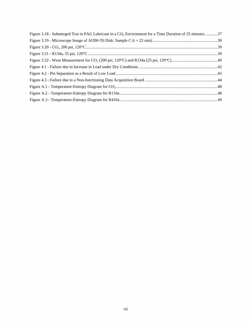
2.4 Experimental Procedure and Conditions The pin-on-disc or the shoe-on-disk geometry was used to carry out the experiments in the HPT. For the

pin-on-disk geometry both samples used were made of gray cast iron. For the shoe on disk geometry the shoes were

made out of 52100 Steel and the disks were Al 390-T6. Typical samples of a disk, pin and shoe are shown in

Figures 2.9 (a) and (b). The samples were prepared with the same machining process and had approximately the

same roughness. The roughness for both the cast iron pins and disks was between 300-500 nm. The roughness of

the Al disks was about 700 nm while the steel shoes were considered infinitely smooth. Some of the early

experiments were performed using pins that were polished. Even though we tried to be consistent in the polishing,

sometimes we noticed variation in the roughness. This may have influenced some of the early results, however, we

tried to repeat the tests several times to ensure repeatability and we have included results that we think are

representative.

All types of tests could be summarized into five categories depending on the experimental conditions.

These five types are described in later sections.

(a) (b)

Figure 2.9 – Typical Samples (a) Disk, (b) Pin and Shoe

Before initiating a test, the samples are pre-screened, optically and by contact profilometry, to ensure they

have minimal surface damage from scratches. Then, the samples are immersed in pools of acetone and

ultrasonically cleaned. They are rinsed with alcohol and dried using warm air. The samples are then placed in

sealed containers to prevent contamination.

The running conditions for the samples in the HPT may vary. Different rotation speed, initial load, step

load, environmental temperature and pressure have been used depending on the type of test. The different test

conditions are described under the sections that correspond to the different types of tests. After the tribological

testing the samples are again ultrasonically cleaned and used for wear quantification and surface topography

measurements

16

2.5 Experimental Setups Under this section five different types of tests are described in detail. These are: Type I-dry, non-lubricated

under the presence of refrigerant, Type II-lubricated using spray of refrigerant only, Type III-lubricated using spray

of refrigerant and lubricant, Type IV-fully submerged in PAG lubricant, and Type V-direct application of PAG

lubricant via an absorbing medium.

The preliminary work of Cusano and Stokes (Cusano 1999) included Type III experiments. This type of

test was developed by Cusano and has been used to accurately simulate the typical compressor conditions and test

the performance of several material interfaces under the presence of refrigerants such as R134a and R410a.

However, due to the difference in the thermodynamic properties, the Type III cannot be used with CO2 as a

refrigerant. That led to Type I and later on Type IV and V to avoid the complications that make the method of Type

III inapplicable.

2.5.1 Preliminary Type I, II and III Experiments There are two sets of preliminary tests. The first set was performed by Cusano and Stokes and the second

set was performed by Poziemski and Reifman. Since the latter preliminary results consist of all types of test, they

are described in detail in Sections 2.5.2 through 2.5.4 below.

In the experiments by Cusano and Stokes the weight of the CO2/PAG mixture was between 405gr and

420gr, approximately 0.05% of which was oil. This corresponds to 40 mg/min and it was determined by trial and

error since higher supply rates would result in no scuffing. Numerous experiments were performed and the test

conditions for Type III of test are as follows:

• Initial normal load and step loading: 10 lbf with 10 lbf/15 sec

• Rotation speeds: 1.86 m/s, 2.79 m/s, 3.72 m/s and 4.65 m/s

• Chamber temperature: 120°C

• Chamber pressures: 25 psi The step duration of 15 seconds is adequate because a steady state temperature is reached after approximately 10

seconds under starved lubrication conditions. When the CO2/PAG mixture was used the tests were occasionally

stopped before scuffing due to the depletion of the mixture in the pressure vessel. The pressure of 25 psi was used

with the assumption that when the two refrigerants are compared, the pressure will not affect the results. Most tests

focused in the use of CO2 since R134a has continuously been used in the past and a great deal of experience has

been obtained.

In the second set of preliminary tests that were performed by Poziemski and Reifman, a comparison

between three different types of tests was investigated. This comparative study included Type I, II and III in CO2

environment. Numerous experiments were performed and the test conditions for all types of test are as follows:


• Rotation speeds: 2.4 m/s and 4.65 m/s

• Chamber temperature: 75°C • Chamber pressures: 50 psi and 200 psi

17

2.5.2 Type I – Dry, Non-Lubricated under Presence of Refrigerant The dry, non-lubricated tests are the simplest from all other types of tests and the preparation process

requires very little time. For this type of test cast iron pins on cast iron disk samples were used. These basic

experiments simulate the worse case scenario in a compressor.

1. The samples are prepared as described above in Section 2.4. 2. A plug is inserted to the base fixture to prevent leaks and also to ensure that a good vacuum is created once

the chamber is closed. That is shown on Figure 2.10. 3. The prepared disk is placed onto the tribometer spindle and the sample pin is placed on the specimen

holder. Then the base fixture is carefully placed inside the chamber. One should ensure that it sits properly and that the ECR cables will not be in the way of the spindle once the chamber closes.

Figure 2.10 - Base Fixture Figure 2.11 - Tribometer Chamber

4. Once the fixture is secured in place and tightened using the screws, the chamber is raised until it is properly closed.

5. The refrigerant is connected to the external HPT port. 6. A vacuum is created using a pump that is connected to the tribometer 7. The chamber is then filled with refrigerant to the required pressure. 8. Then the pin is brought in contact with the disk with an initial load of 10 lbf. 9. Through the computer, the test is initiated.

The test conditions for this type of test are as follows:

• Initial normal load and step loading: 15 lbf with no step • Rotation speed: 1030 RPM (2.4 m/s)

• Temperature: 0°C, 60°C, 120°C

• Chamber pressures: 50 psi and 200 psi These conditions are selected is via numerous trials under a chosen environmental condition. It was decided that a

load of about 17 lbf is reasonable since the material and the given geometry don’t allow for a higher load. Any load

higher than 20 lbf would lead to immediate failure. Three different temperatures and two different pressures were

selected for comparison.

Plug

Base fixture

Chamber

18

2.5.3 Type II- Lubricated Using Spray of Refrigerant This type of test is more complicated and much more time consuming than Type I. Type II should provide

similar tribological performance as Type I and possibly better since the contact has a continuous flow of refrigerant.

The weight and pressures below refer to the case of CO2 and for other refrigerants would be significantly lower.

However, the methodology is the same no matter what refrigerant one uses.

The following steps are necessary before every test using spray of refrigerant only:

1. A pressure vessel is rinsed with a few drops of 2-propanol and the contents are driven out with compressed air. When empty it should approximately weigh 6500 gr.

2. The empty vessel is then immersed in an ice bath. 3. The vessel is connected to a greater cylinder containing the refrigerant and the fill-up process begins. 4. After fill-up, the weight of the pressure vessel should be around 8250 gr. That means the weight of the

refrigerant is 1750 gr. The pressure after fill up is around 800 psi. 5. The vessel is mounted on the HPT and connected to the inlet. 6. A heating blanket is attached to the vessel and the contents are heated at a voltage of 40% to 1520 psi as

seen in Figure 2.12 below. 7. It is recommended that no more than a voltage of 50% be used to reduce the risk of burning the fuse. To

achieve 1520 psi the heating process takes approximately forty minutes at 40%. The temperature of the contents at this pressure is approximately 70°C. At this point CO2 is entirely in its gaseous phase as seen in the phase diagram presented earlier in Figure 1.1.

8. A nozzle is inserted to the base fixture to spray the refrigerant during the test. 9. Follow steps 3 through 6 of Section 2.5.2. 10. The spindle is set to rotate and the refrigerant is sprayed to lubricate the surface. This is done

simultaneously ensuring that the pressure chamber gauge is kept under control so that the required pressure is not exceeded.

Figure 2.12 - Heating of the Pressure Vessel

11. Then the pin is brought in contact with the disk with an initial load of 10 lbf. 12. Through the computer, the test is initiated.

19


• Initial normal load and step loading: 15 lbf with no step

• Rotation speed: 1030 RPM (2.4 m/s) • Temperature: Typically 75°C

• Chamber pressures: 50 psi and 200 psi For this series of tests the shoe-on-disk geometry was used. Only a very limited amount of such tests was performed

to examine how they compare to the Type I- dry, non-lubricated test. However, this type is also very aggressive and

any load higher than 20 lbf would lead to immediate failure of the material for the shoe on disk geometry.

2.5.4 Type III-Lubricated Using Spray of Lubricant and Refrigerant This type of test is very similar to a Type II-Lubricated using spray of refrigerant only, with the exception

that a small amount of lubricant is added into the pressure vessel before the refrigerant. The motivation for this type

of test is that it simulates typical compressor conditions where a small amount of lubricant reaches the surface.

After step 1 in Section 2.5.3, 5 mg of lubricant is weighted and then added to the clean pressure vessel. The vessel is

placed into an ice bath and steps 3-12 are followed. For this series of tests the shoe-on-disk geometry was used.


• Initial normal load and step loading: 10 lbf with a step increase of 10 lbf/15 seconds

• Rotation speed: 1030 RPM (2.4 m/s) and 2000RPM (4.65 m/s)

• Temperature: 75°C

• Chamber pressures: 50 psi and 200 psi

2.5.5 Type IV-Fully Submerged in PAG Lubricant This test requires a lot of care due to several reasons that will be described below. It serves as an ideal

compressor case.

1. A plug is inserted to the base fixture as done previously in Section 2.5.2. 2. Then a tight fit of the glass around the base fixture is needed to ensure that no lubricant will leak out once

the glass is filled with lubricant. 3. The prepared sample disk is placed onto the tribometer spindle and the sample pin or shoe is placed on the

fixture. 4. The fixture is secured in place and tightened using the screws along with o-rings around the screws to

prevent leakage. 5. Using a funnel, the desired lubricant is carefully poured into the glass until the specimen holder is fully

covered and the pin or shoe, depending on the experiment, is completely submerged. 6. Then the chamber is raised until it is properly closed. 7. Follow steps 5-8 of Section 2.5.2. Note that when the vacuum check is initiated the oil starts bubbling.

Basically the air that was trapped inside the oil starts coming out. The vacuum check will be complete even though air bubbles will continue coming out of the oil.

8. Through the computer, the test is initiated.


• Initial normal load and step loading: 50 lbf with a step increase of 100 lbf/2.5 minutes

• Rotation speed: 1030 RPM (2.4 m/s) • Temperature: 90°C

• Chamber pressures: 200 psi

20

These conditions were also selected via several test trials. Even though these conditions are very aggressive there is

hardly any detectable wear on the disk. So, a lower load is not recommended. Different times were performed for

this type of tests to see the progressive wear pattern (Patel, 2000). However, no scuffing was attained with such

experiments.

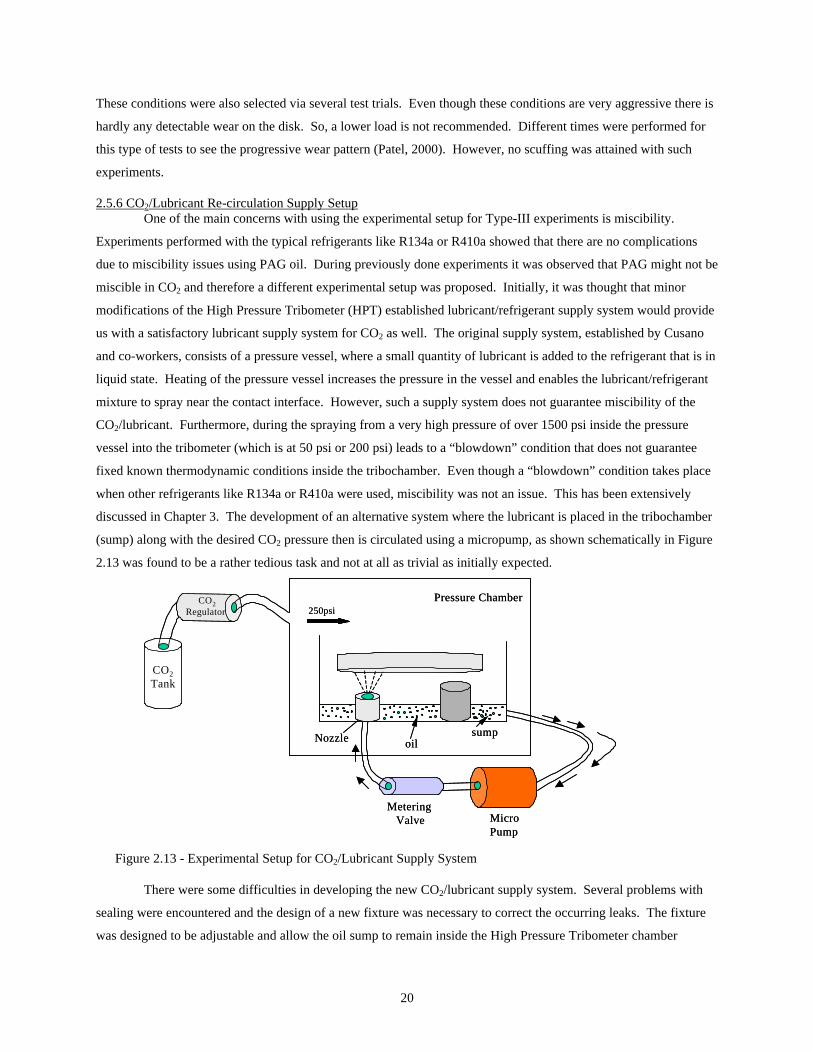
2.5.6 CO2/Lubricant Re-circulation Supply Setup One of the main concerns with using the experimental setup for Type-III experiments is miscibility.

Experiments performed with the typical refrigerants like R134a or R410a showed that there are no complications

due to miscibility issues using PAG oil. During previously done experiments it was observed that PAG might not be

miscible in CO2 and therefore a different experimental setup was proposed. Initially, it was thought that minor

modifications of the High Pressure Tribometer (HPT) established lubricant/refrigerant supply system would provide

us with a satisfactory lubricant supply system for CO2 as well. The original supply system, established by Cusano

and co-workers, consists of a pressure vessel, where a small quantity of lubricant is added to the refrigerant that is in

liquid state. Heating of the pressure vessel increases the pressure in the vessel and enables the lubricant/refrigerant

mixture to spray near the contact interface. However, such a supply system does not guarantee miscibility of the

CO2/lubricant. Furthermore, during the spraying from a very high pressure of over 1500 psi inside the pressure

vessel into the tribometer (which is at 50 psi or 200 psi) leads to a “blowdown” condition that does not guarantee

fixed known thermodynamic conditions inside the tribochamber. Even though a “blowdown” condition takes place

when other refrigerants like R134a or R410a were used, miscibility was not an issue. This has been extensively

discussed in Chapter 3. The development of an alternative system where the lubricant is placed in the tribochamber

(sump) along with the desired CO2 pressure then is circulated using a micropump, as shown schematically in Figure

2.13 was found to be a rather tedious task and not at all as trivial as initially expected.

sumpoilNozzle

CO2Tank

CO2Regulator 250psi

Pressure Chamber

MeteringValve Micro

Pump

sumpoilNozzle

CO2Tank

CO2Regulator 250psi

Pressure Chamber

MeteringValve Micro

Pump Figure 2.13 - Experimental Setup for CO2/Lubricant Supply System

There were some difficulties in developing the new CO2/lubricant supply system. Several problems with

sealing were encountered and the design of a new fixture was necessary to correct the occurring leaks. The fixture

was designed to be adjustable and allow the oil sump to remain inside the High Pressure Tribometer chamber

21

without leaking. Filter selection was another really important issue that had to be resolved. As the pin and disk

make contact, there is debris that can be potentially harmful for the pump so a 10-micron stainless steel filter

becomes necessary before the inlet of the gear pump. Two filters were used. Both of these filters were ordered from

Upchurch Scientific. The first one was made out of PEEK. This filter can draw solvent to within 2 mm of the

bottom of the solvent bottle. The maximum flow rate of the 10 mm filter is 100 ml/min. The part number for this

filter is A-438. The second filter was made out of 316 stainless steel. This filter can draw solvent to within 3.2 mm

of the bottom. The part number for this filter is A-550. In order to use, we simply press fit the Teflon tubing firmly

into the top holes.

(a) (b)

Figure 2.14 - Filters Used in the Re-circulation Setup (a) PEEK (b) Stainless Steel

Figure 2.15 - Modified Fixture for New Lubricant/CO2 Supply System

However, due to space limitations, as it can be seen in Figure 2.15, a longer pin holder had to be designed

to allow full submersion of the filter while the pin is not submerged as pointed out with a green arrow in the same

figure. In this figure we can also see a special adapter (red circle) for extending the nozzle above the level of the oil

so that it is not submerged when the filter is fully submerged.

Furthermore, many different adapters, connectors and pipes had to be selected to create a setup that would

be compatible with both the HPT and existing pumps. During this stage, two types of pumps were tested. These

were a piston pump and a gear pump. The piston pump was quickly eliminated even though it provides very small

flow rates because a continuous flow was needed. Experiments with the gear pump were attempted but the setup

still needed some refinements. The orifice size of the nozzle was also another issue that could not be resolved. That

creates a pressure built up in the outlet and along the lines of the pump that results in leakage through the pump.

Filter

22

This setup did not work because of the high pressure differential needed to pump the oil back into the

chamber as an atomized spray, so no results have been obtained.

2.5.7 Type V-Direct Application of PAG Lubricant via Absorbing Medium This type of experiment requires special care since there is no previous experience with the setup used.

This is perhaps the “ideal” experiment. The need for boundary and mixed lubrication with CO2 is fulfilled and

stable thermodynamic conditions are achieved. The following steps are needed:

1. We cut an absorbing medium with approximate diameter of 2.5 inches. This is a commercially available type of woven cloth with a medium density.

2. The medium is inserted inside a holder and tightened on the base fixture as shown in Figure 2.16 below. 3. We ensure that the height of the cloth is slightly higher than the specimen holder so that it will make

contact with the disk before the pin. However, it is important to ensure that the cloth does not exceed a certain height, as this will cause a lot of damage to the cloth once the disk starts rotating.

4. We measure approximately 50 mg of PAG lubricant in a beaker and with a syringe we apply the oil to the absorbing medium. This corresponds to 3 drops of lubricant using a regular syringe.

5. We follow steps 2 through 7 of Section 2.5.2. 6. Then we bring the absorbing medium in contact with the disk and allow the disk to rotate a couple of times

to get a lubricant film on the disk. 7. Then we bring the pin into contact with the disk with an initial load of 20 lbf.

Figure 2.16 - Setup for Direct Application of Lubricant via Absorbing Medium

8. Through the computer, the test is initiated. The test conditions for this type of test are as follows:


• Rotation speed: 1030 RPM (2.4 m/s)

• Temperature: 120°C

23

• Refrigerant: R134a, CO2

• Chamber pressures: 25 psi (R134a), 200 psi (CO2) Through trial and error it was realized that approximately 50 mg of oil is adequate to create a lubricant film. The

ECR was a useful indicator to realize that 50 mg is the amount needed since it places the contact in the mixed

boundary lubrication regime. If more oil is used, there is no detectable wear even with very high loads. The loading

conditions were also selected via numerous trials. Aggressive conditions are needed and the chosen 35 lbf/30 sec

increase seems to be satisfactory for the amount of oil used for this test. R134a was selected for the comparison.

24

Chapter 3. Results and Discussion

3.1 Introduction All of the 5 different types of tests were performed in order to better understand the behavior of CO2 and

how it compares with other refrigerants. Due to the thermodynamic complexities involved in Types II and III and

the discrepancies observed in some preliminary work during the Type III test, we tried to isolate some of the

thermodynamics, which initially led us to performing Type I and later on Type IV and V tests.

The Type III test was developed more than a decade ago by Cusano and has extensively been used in the

past to test the performance of numerous material interfaces under the presence of refrigerants such as R134a and

R410a. However, it was never used with CO2 as a refrigerant. As previously mentioned in Chapter 1, CO2 is

thermodynamically much different than the refrigerants above, for which a great deal of knowledge has been gained

by the continuous work with them. When involvement with CO2 was engaged it was not anticipated that it would be

much different and that the previously developed method for testing could be applied as well. Unfortunately, this

was not true. The existing method could not be applied to CO2 and the reason for that was immiscibility coupled

with the fact that under the conditions used for spraying in a Type III test, CO2 was in its gaseous state unlike the

other refrigerant which were in liquid state. In the preliminary work, the importance of miscibility was not realized

and numerous experiments were performed using the setup described in Section 2.5.4. These have been discussed

below.

After the basic Type I tests, the issue of miscibility had to be examined. The initial thought was to deliver

the oil in the surface separately while the chamber was in the presence of refrigerant. So a re-circulation setup was

proposed that would have the lubricant in a sump and then through a pump we would provide it to the surface while

the chamber was pressurized with refrigerant. After some effort it was realized that due to the high pressure

differentials needed to pump the oil back into the chamber as an atomized spray this setup cannot work. That led to

Type IV and V tests.

3.2 Preliminary Experiments-Main findings

3.2.1 Cusano-Stokes Experiments (1999) The scuffing resistance of R134a was compared to CO2 under the presence of PAG lubricant. Consistent

data could not be acquired for the tests conducted using a CO2/PAG mixture and a satisfactory explanation for the

inconsistency could not be offered. It was proposed that this inconsistency is due to lack of understanding of CO2 in

the system. However, it was noted that in spite of the scatter within the data, the results indicated that the CO2/PAG

mixture has better lubricative properties than the R134a/PAG mixture. During this work it was observed that the

friction during the progression of the tests utilizing the CO2/PAG mixture was lower than the tests using the

R134a/PAG mixture.

The curve for CO2 could not be fitted due to the large scatter as well as the high number of tests that did not

scuff before the CO2/PAG mixture ran out. On the other hand, the scuffing data for R134a/PAG mixture maintained

an approximate PV=constant relationship. As the sliding velocity increases, the scuffing pressure decreases.

Despite the scatter, a similar trend was ascertained from the CO2/PAG data. For the same velocity nearly all results

25

failed at pressures higher than the scuffing pressures using R134a. The results can be seen in Figure 3.1 where a

pressure-velocity diagram is presented for the two mixtures.

As we previously mentioned, immiscibility is the most probable reason that makes this method for testing

under the presence of CO2 inappropriate. After the filling process, CO2 exists inside the pressure vessel as liquid

and gas. So, initially the liquid CO2 is mixed with the lubricant but as the heating process takes place to raise the

pressure so that it can be sprayed, the liquid CO2 turns into gas and the lubricant remains on the bottom of the vessel.

A possible explanation to what follows is that when the valve is opened and the contents are sprayed, the

lubricant comes out all at once first, and then CO2 gas is continuously sprayed coming out of the nozzle as dry ice

that instantly turns again into gas since the chamber temperature is high.

Figure 3.1 - Scuffing Pressure-Velocity Diagram for Al 390-T6 and 52100 Steel in R134a/PAG or CO2/PAG

In the preliminary results by Cusano and Stokes it is almost evident that this is what takes place in the

results obtained for CO2 from the low coefficients of friction achieved. When the lubricant is initially sprayed onto

the surface it takes quite some time until scuffing and since the lubricant/refrigerant spray is not uniform during the

duration of the test like in the case of R134a but comes out all at once, the friction coefficient remains low.

3.2.2 Poziemski-Reifman Experiments (Summer 2001) During the preliminary work by Poziemski and Reifman, Type I, II and III were performed to further

investigate the previously observed scatter in the data by Cusano and Stokes. The methodology and the way this

experiments were carried was once again the same as the method utilized by Cusano and Stokes. For Type II and III

the refrigerant undergoes the same phase changes when heated and sprayed. From its initial two phase (liquid and

26

gas) it is heated at which point there is only gas and then sprayed becoming dry ice that quickly turns into gas due to

the high chamber temperature. So, these series of tests resulted in scatter for Type III as we could have expected for

the same reasons as previously explained in section 3.2.1. The thermodynamics are the same for the Type II tests as

well.

All three types of experiments (I, II, and III) were performed at 2 different speeds (2.4 m/s and 4.65 m/s)

and are depicted in a P-V diagram in Figure 3.2 below. Each point in the graph corresponds to a single experiment.

0

10

20

30

40

50

60

70

0 1 2 3 4 5

Sliding Velocity (m/s)

Ave

rag

e C

on

tact

Pre

ssu

re, P

(M

Pa)

2.4m/s 50psi Type(III) (4pts)

2.4m/s 50psi Type(II) (2pts)



2.4m/s 200psi Type(I) (2pts)



4.65m/s 200psi (TypeII) (3pts)

4.65m/s 200psi Type(I) (2pts)

Figure 3.2 - Scuffing Pressure-Velocity Diagram for Al 390-T6 and 52100 Steel in CO2/POE

The average contact pressure on the y-axis corresponds to the maximum normal load at which scuffing

occurred divided by the nominal contact area. If we closely examine Figure 3.2, we can observe that consistent data

occur only for Type I and II experiments. For 2.4 m/s, Type I (CO2 presence alone) and Type II (CO2 spray)

experiments produce very repeatable data points, where scuffing occurred at the pressures of about 3 MPa, and 13

MPa, respectively. On the other hand, for Type III experiments (CO2/POE spray) the results of three experiments

are not very repeatable with scuffing varying between 20-37 MPa. When the same experiments were repeated at the

higher speed of 4.65 m/s, the repeatability is once again seen for Type I and II experiments only. For Type III

experiments, the two experiments that were performed produce very different results.

So, Type III experiments exhibit large scatter, similar to the scatter reported by Cusano and Stokes using

CO2/PAG oil. From the experiments above we note that the performance of Type III is better than Type II, which,

in turn is better than Type I. The consistency of Type I experiments gave the motivation for the next experiments

described in Section 3.3.

27

3.3 Type I-Dry, Non-Lubricated under Presence of Refrigerant In order to avoid the aforementioned thermodynamic complexities, Type I experiments were conducted.

This is a very basic type of experiments that was performed in order to better understand the behavior of CO2 and

also compare its lubricative properties with previously used refrigerants. The cast iron pin-on-disk geometry was

used for these tests.

During this type of test, there is no phase change since the chamber pressure is constant at a known fixed

value. There are no thermodynamics involved during this type of test and the conditions (temperature and pressure)

are known at any give time. Nonetheless, a drawback with this type of test is that the absence of lubricant does not

allow for high loads and only very low loads can be sustained by the material interfaces used in this work. This is

the worse case scenario for compressors.

Numerous experiments of this type were performed. The early experiments were performed using pins that

were polished and in many instances there was variation in the roughness. This may have influenced some of the

early results, however, we tried to repeat the tests several times to ensure repeatability and we have included results

that we think are representative. First we studied the effects of temperature and pressure and then we compared CO2

with R134a and air.

3.3.1 Effects of Temperature and Pressure Three different temperatures namely 0°C, 60°C and 120°C selected as low, medium and high respectively,

while two different pressures, 50 psi and 200 psi, as low and high respectively were examined. For the case of 50

psi we can see the effect of temperature in our results. This can be seen in Figures 3.3 through 3.5 below. At 0°C,

the coefficient of friction is low taking values between 0.1 and 0.25 while the near-contact temperature also remains

low around 50°C. At 60°C, the coefficient of friction is higher than the 0°C case taking a value of about 0.5 while

the near-contact contact temperature is significantly higher this time with a value of about 200°C. For the case of

120°C, the friction coefficient is the highest from the other two cases taking a value of about 1 while the contact

temperature reaches 300°C.

So, for the case of the lower pressure of 50 psi the results seem to indicate that as temperature increases, the

coefficient of friction and the near-contact temperature both increase. That is what one could have expected at this

range of temperatures. For the case of 0°C it is possible that water due to condensation was acting as a lubricant

creating a film between the interacting surfaces. Condensation was visible before initiation and during the

experiment. However, for the case of 60°C and 120°C there was no condensation, and the results seem to follow the

expected trend.

28

0 1 2 3 4 5 6 7 8 9 1005

101520

Load

(lbf)

0 1 2 3 4 5 6 7 8 9 100

0.250.5

0.751

µ r

0 1 2 3 4 5 6 7 8 9 100

100200300400

Tem

pera

ture

(o C)

0 1 2 3 4 5 6 7 8 9 1010

-210

-110

010

110

2

EC

R(O

hms)

Time (min)

Figure 3.3 - CO2, 50 psi, 0°C

0 1 2 3 4 5 6 7 8 9 1005

101520

Load

(lbf)

0 1 2 3 4 5 6 7 8 9 100

0.250.5

0.751

µ r

0 1 2 3 4 5 6 7 8 9 100

100200300400

Tem

pera

ture

(o C)

0 1 2 3 4 5 6 7 8 9 1010

-210

-110

010

110

2

EC

R(O

hms)

Time (min)


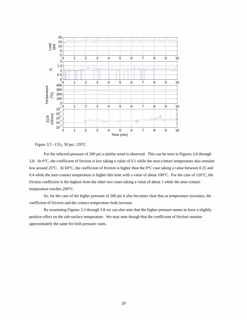
29

0 1 2 3 4 5 6 7 8 9 1005

101520

Load

(lbf)

0 1 2 3 4 5 6 7 8 9 100

0.51

1.52

µ r

0 1 2 3 4 5 6 7 8 9 100

100200300400

Tem

pera

ture

(o C)

0 1 2 3 4 5 6 7 8 9 1010

-210

-110

010

110

2

EC

R(O

hms)

Time (min)

Figure 3.5 - CO2, 50 psi, 120°C

For the selected pressure of 200 psi a similar trend is observed. This can be seen in Figures 3.6 through

3.8. At 0°C, the coefficient of friction is low taking a value of 0.1 while the near-contact temperature also remains

low around 25°C. At 60°C, the coefficient of friction is higher than the 0°C case taking a value between 0.25 and

0.4 while the near-contact temperature is higher this time with a value of about 100°C. For the case of 120°C, the

friction coefficient is the highest from the other two cases taking a value of about 1 while the near-contact

temperature reaches 200°C.

So, for the case of the higher pressure of 200 psi it also becomes clear that as temperature increases, the

coefficient of friction and the contact temperature both increase.

By examining Figures 3.3 through 3.8 we can also note that the higher pressure seems to have a slightly

positive effect on the sub-surface temperature. We may note though that the coefficient of friction remains

approximately the same for both pressure cases.

30

0 1 2 3 4 5 6 7 8 9 1005

101520

Load

(lbf)

0 1 2 3 4 5 6 7 8 9 100

0.250.5

0.751

µ r

0 1 2 3 4 5 6 7 8 9 100

255075

100

Tem

pera

ture

(o C)

0 1 2 3 4 5 6 7 8 9 1010

-210

-110

010

110

2

EC

R(O

hms)

Time (min)


0 1 2 3 4 5 6 7 8 9 1005

101520

Load

(lbf)

0 1 2 3 4 5 6 7 8 9 100

0.250.5

0.751

µ r

0 1 2 3 4 5 6 7 8 9 100

100200300400

Tem

pera

ture

(o C)

0 1 2 3 4 5 6 7 8 9 1010

-210

-110

010

110

2

EC

R(O

hms)

Time (min)

Figure 3.7 - CO2, 200 psi, 60°C

31

0 1 2 3 4 5 6 7 8 9 1005

101520

Load

(lbf)

0 1 2 3 4 5 6 7 8 9 100

0.51

1.52

µ r

0 1 2 3 4 5 6 7 8 9 100

100200300400

Tem

pera

ture

(o C)

0 1 2 3 4 5 6 7 8 9 1010

-210

-110

010

110

2

EC

R(O

hms)

Time (min)

Figure 3.8 - CO2, 200 psi, 120°C

0

0.2

0.4

0.6

0.8

1

1.2

0 60 120Chamber Temperature (oC)

Fric

tion

Coe

ffici

ent 50 psi

200 psi

Figure 3.9 - Friction Coefficients for Constant Load Tests for CO2 at Different Operating Conditions

32

0

50

100

150

200

250

300

350

0 60 120Chamber Temperature (oC)

Con

tact

Tem

pera

ture

(o C)

50 psi200 psi

Figure 3.10 - Contact Temperatures for Constant Load Tests for CO2 at Different Operating Conditions

Two experiments for each of the different conditions were performed. In general, the results were similar

and we believe we have included representative tests. However, one should keep in mind that it is possible that

some of these tests were performed using samples that were not identically prepared. Roughness variations are

likely to have occurred due to polishing and some disks may not have had the coating mentioned above.

The results for the different pressures and temperatures have been summarized in Figures 3.9 and 3.10.

3.3.2 Comparison of CO2 with R134a and air The test protocol developed more than a decade ago by Cusano and co-workers that has extensively been

used in the past to test the performance of numerous material interfaces under the presence of refrigerants such as

R134a was never used with CO2 as a refrigerant. As previously mentioned, CO2 is thermodynamically much

different than commonly used refrigerants. The existing method could not be applied to CO2 and the reason for that

was immiscibility of lubricant coupled with the fact that under the conditions used for spraying, CO2 was in its

gaseous state unlike the other refrigerants, which were in liquid state. In order to avoid the issue of immiscibility,

controlled experiments at constant loads in the presence of CO2, R134a and air were performed. CO2 was compared

with refrigerant R134a and air under Type-I, dry non-lubricated test. R134a was tested at 60°C and 25 psi the same

way CO2 was tested at 50 psi. Air was tested at ambient pressure and 60 °C. The results obtained for CO2 are

shown in Figure 3.11 while the results for R134a are shown in Figure 3.12. If we compare the two figures we will

see that the two refrigerants performed quiet similarly.

33

0 0.5 1 1.5 2 2.5 3 3.5 4 4.5 505

101520

Load

(lbf)

0 0.5 1 1.5 2 2.5 3 3.5 4 4.5 50

0.250.5

0.751

µ r

0 0.5 1 1.5 2 2.5 3 3.5 4 4.5 50

100200300400

Tem

pera

ture

(o C)

0 0.5 1 1.5 2 2.5 3 3.5 4 4.5 510

-5

100

105

EC

R(O

hms)

Time (min)

Figure 3.11 - CO2, 50 psi, 60°C

0 0.5 1 1.5 2 2.5 3 3.5 4 4.5 505

101520

Load

(lbf)

0 0.5 1 1.5 2 2.5 3 3.5 4 4.5 50

0.250.5

0.751

µ r

0 0.5 1 1.5 2 2.5 3 3.5 4 4.5 50

100200300400

Tem

pera

ture

(o C)

0 0.5 1 1.5 2 2.5 3 3.5 4 4.5 510

-5

100

105

EC

R(O

hms)

Time (min)

Figure 3.12 - R134a, 25 psi, 60°C

34

0 0.5 1 1.5 2 2.5 3 3.5 4 4.5 505

101520

Load

(lbf)

0 0.5 1 1.5 2 2.5 3 3.5 4 4.5 50

1

2

3

µ r

0 0.5 1 1.5 2 2.5 3 3.5 4 4.5 50

100200300400

Tem

pera

ture

(o C)

0 0.5 1 1.5 2 2.5 3 3.5 4 4.5 510

-5

100

105

EC

R(O

hms)

Time (min)

Figure 3.13 - Air, 60°C

The coefficient of friction in the case of CO2 with a value of 0.5 is very similar to the one exhibited under

the presence R134a. On the other hand, in the presence of air, the results are significantly different. The coefficient

of friction starts out high at a value of about 1 and continuously increases to a value of 2 at the end of the test of 5

minutes. This can be seen in Figure 3.13. We may also note is that the near-contact temperature in the case of CO2

is about the same as in the case of R134a taking a value of approximately 100°C. The contact temperature in the

presence of air was unstable and increased from an initial value of 200°C to 300°C at the end of the test. From these

experiments the positive effect of refrigerant can be seen.

Wear measurements for these experiments were taken. Theses are shown in Figure 3.14, for CO2, R134a

and air. They have been included in the same figure for direct comparison. As we can see the wear is higher in the

case of air where the wear depth is approximately 4 µm whereas for CO2 and R134a the wear depth is approximately

2µm. This is what one would have expected, since generally, wear increases with increasing coefficient of friction.

35

0 1 2 3 4 5 6 7 8 9 10-20

-10

0

-10

0

-10

0

10

Scan Length (mm)

Wea

r Dep

th ( µ

m)

CO2

R134a

Air

Wear Scar

Figure 3.14 - Wear Measurement for CO2, R134a and air, 50 psi, 60°C

Wear was also quantified in terms of the pins. The results for CO2, R134a and air are shown in Table 3.1.

The final weight of the pins tested in CO2 and R134a environments is similar whereas the final weight of the pin

tested in air decreased significantly.

A summary of the experimental conditions and the results obtained for CO2, R134a and air compared under

dry conditions is shown in Table 3.1.

Table 3.1 experimental conditions and results obtained for CO2, R134a and air

Refrigerant CO2 R134a Air Chamber Pressure ( psi) 50 25 14.5

Chamber Temperature (°C) 60 60 60 Load (lbf) 14 14 14

Linear Speed (m/s) 2.4 2.4 2.4 Before 1.407 1.408 1.407

Pin weight (g) After 1.395 1.393 1.330

Pin Wear (g) 0.012 0.015 0.077 Near-contact Temperature (°C) 90-130 100-150 200-300

0.5 0.5 1-2 Friction Coefficient

Constant Constant Increasing

3.4 Type IV-Fully Submerged in PAG Lubricant The issue of immiscibility was once again resolved by completely submerging the contacting surfaces in

lubricant and simply pressurizing the chamber with refrigerant. So, once again we had known fixed thermodynamic

conditions just like the Type I tests. That initiated Type IV experiments which are similar to Type I, but in the

presence of lubricant. These experiments simulate ideal compressor conditions. Under these conditions, the

36

coefficient of friction remains very low and there is no detectable wear on the disks after the experiments. Very

high loads and long time durations were needed in order to see minor wear or burnishing. The shoe-on-disk (Steel

52100 on Al 390-T6) geometry was used for these tests.

0 1 2 3 4 5 6 7 8 9 100

100

200

300

400

Load

(lbf)

0 1 2 3 4 5 6 7 8 9 100

0.05

0.1

0.15

0.2

µ r

0 1 2 3 4 5 6 7 8 9 100

30

60

90

120

Tem

pera

ture

(o C)

Time (min)

Figure 3.15 – Submerged Test in PAG lubricant in a CO2 Environment for a Time Duration of 10 minutes

0 2 4 6 8 10 12 14 16 18 200

250

500

750

1000

Load

(lbf)

0 2 4 6 8 10 12 14 16 18 200

0.05

0.1

0.15

0.2

µ r

0 2 4 6 8 10 12 14 16 18 200

30

60

90

120

Tem

pera

ture

(o C)

Time (min)

Figure 3.16 – Submerged Test in PAG lubricant in a CO2 Environment for a Time Duration of 20 minutes

37

0 2 4 6 8 10 12 14 16 18 20 220

250

500

750

1000

Load

(lbf)

0 2 4 6 8 10 12 14 16 18 20 220

0.05

0.1

0.15

0.2

µ r

0 2 4 6 8 10 12 14 16 18 20 220

30

60

90

120

Tem

pera

ture

(o C)

Time (min)

Figure 3.17 - Submerged Test in PAG Lubricant in a CO2 Environment for a Time Duration of 22 minutes

0 2 4 6 8 10 12 14 16 18 20 22 24 250

250

500

750

1000

Load

(lbf)

0 2 4 6 8 10 12 14 16 18 20 22 24 250

0.05

0.1

0.15

0.2

µ r

0 2 4 6 8 10 12 14 16 18 20 22 24 250

30

60

90

120

Tem

pera

ture

(o C)

Time (min)

Figure 3.18 - Submerged Test in PAG Lubricant in a CO2 Environment for a Time Duration of 25 minutes

It is our understanding that companies routinely perform tests under these conditions, where refrigerant is

usually provided near the contact under atmospheric conditions using a “bubbling” method.

38

Several fully submerged tests were performed using PAG oil and CO2. For each experiment, progressively

higher normal loads were imposed for selected time durations. The time durations for these tests were 10 minutes,

20 minutes, 22 minutes, and 25 minutes. The results can be seen below on Figures 3.15 through 3.18.

Due to the fact that the specimens were fully submerged in PAG oil, both the coefficient of friction and the

near-contact temperature have remained very low. These types of tests simulate ideal compressor conditions.

A microscope image for the sample tested for 22 minutes is shown in Figure 3.19. The image of this disk is

similar to the images of the scuffing experiments that were analyzed by (Pergande, 2003). There is no significant

wear and all disks after the tribological testing seem to undergo minute wear or burnishing.

Figure 3.19 - Microscope Image of Al390-T6 Disk: Sample C (t = 22 min)

No definite conclusions can be drawn from the series of the submerged tests. The reason for this is that

actual scuffing time cannot be obtained due to the idealistic conditions of the contact being submerged in lubricant.

3.5 Type V-Direct Application of PAG Lubricant via Absorbing Medium The idealistic case of Type IV tests led us to the development of Type V tests, which is the final type of

experiments presented in this work. The idea behind the development was still the same as before with Type III.

Resolve the issue of immiscibility, but create a more realistic environment for testing. The amount of oil had to be

reduced and reasonably high loads would have to provide us with scuffing results that could be quantified. That was

made possible by directly applying lubricant to the contact by means of an absorbing medium. Every time the disk

rotated the contact was lubricated and the lubrication was in the mixed boundary and mixed regime, which indicated

that there is a load, at which scuffing can occur. The cast iron pin-on-disk geometry was used for these tests.

3.5.1 Comparison of CO2 with R134a This is the most realistic case and we believe that the simplicity and the consistency in the results obtained

can provide us with qualitative results for a comparative study, and the results seem to support that. The effect of

using different refrigerant was examined once again but in the presence of PAG lubricant. CO2 was compared to

39

R134a. As we can see from Figures 3.20 and 3.21, scuffing occurred right at 8 minutes for both refrigerants under

the same conditions.

The friction is the same for both cases as well. It remained low taking a constant value of 0.1 for the

duration of the test until scuffing at which point it increased dramatically.

0 1 2 3 4 5 6 7 8 90

200400600800

Load

(lbf)

0 1 2 3 4 5 6 7 8 90

0.10.20.30.4

µ r

0 1 2 3 4 5 6 7 8 90

50100150200

Tem

pera

ture

(o C)

0 1 2 3 4 5 6 7 8 9Time (min)

EC

R(O

hms) 102

100

10-2

Figure 3.20 - CO2, 200 psi, 120°C

0 1 2 3 4 5 6 7 8 90

200400600800

Load

(lbf)

0 1 2 3 4 5 6 7 8 90

0.10.20.30.4

µ r

0 1 2 3 4 5 6 7 8 90

50100150200

Tem

pera

ture

(o C)

0 1 2 3 4 5 6 7 8 9

EC

R(O

hms)

Time (min)

102

10-2

100

Figure 3.21 - R134a, 25 psi, 120°C

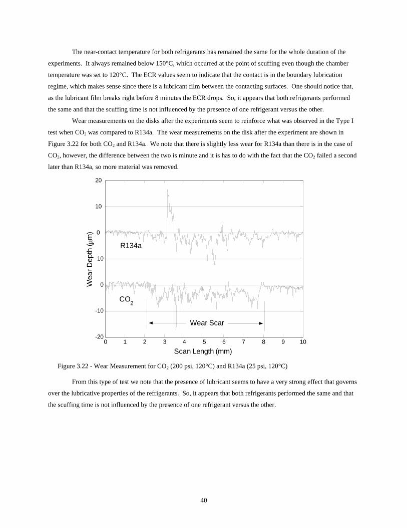
40

The near-contact temperature for both refrigerants has remained the same for the whole duration of the

experiments. It always remained below 150°C, which occurred at the point of scuffing even though the chamber

temperature was set to 120°C. The ECR values seem to indicate that the contact is in the boundary lubrication

regime, which makes sense since there is a lubricant film between the contacting surfaces. One should notice that,

as the lubricant film breaks right before 8 minutes the ECR drops. So, it appears that both refrigerants performed

the same and that the scuffing time is not influenced by the presence of one refrigerant versus the other.

Wear measurements on the disks after the experiments seem to reinforce what was observed in the Type I

test when CO2 was compared to R134a. The wear measurements on the disk after the experiment are shown in

Figure 3.22 for both CO2 and R134a. We note that there is slightly less wear for R134a than there is in the case of

CO2, however, the difference between the two is minute and it is has to do with the fact that the CO2 failed a second

later than R134a, so more material was removed.

0 1 2 3 4 5 6 7 8 9 10-20

-10

0

-10

0

10

20

Scan Length (mm)

Wea

r Dep

th ( µ

m)

CO2

R134a

Wear Scar

Figure 3.22 - Wear Measurement for CO2 (200 psi, 120°C) and R134a (25 psi, 120°C)

From this type of test we note that the presence of lubricant seems to have a very strong effect that governs

over the lubricative properties of the refrigerants. So, it appears that both refrigerants performed the same and that

the scuffing time is not influenced by the presence of one refrigerant versus the other.

41

Chapter 4. Experimental Uncertainties and Techniques

4.1 Experimental Techniques In this chapter, some of the problems encountered during this work have been summarized, which is

intended to serve as a guide for experimental testing and emphasizes the things one should be looking after or avoid

doing. Also some experimental techniques have been suggested to help making the experiments run smoothly while

avoiding complications.

Many times during the setup of a specific type of test, decisions have to be made as to what the load should

be for given environmental conditions so that the given geometry and the material could withstand the load. The

way the load was selected was by numerous trials under a selected environmental condition. An important factor

was also whether the load application should be constant or increased in a step-loading manner. If a standard wear

test is preferred, then a constant load is applied. A step-loading test allows us to test to failure (scuffing).

When no lubricant is present the decision of what the load should is difficult since it has been observed that

a material pair may scuff at very low loads. On the other hand, when lubricant is present, scuffing will only occur at

very high loads. During this work two different material interfaces were studied, Al 390-T6 and cast iron. The

shoe-on-disk geometry of Steel 52100 shoes on Al 390-T6 disks was used only under the Type IV-fully submerged

in PAG lubricant tests. However, a great deal of experience has been gained by working with the pin-on-disk

geometry of cast iron pins on cast iron disks through both lubricated and non-lubricated tests. Load selection for

these are discussed in the sub-sections below.

4.1.1 Load Selection for Type I-Dry, Non-Lubricated Tests Typically, under dry conditions, without the presence of lubricant, the load that can be sustained from the

pin-on-disk geometry using different materials is very low. The materials tested during this work as previously

mentioned were cast iron pins on cast iron disks, and Steel 52100 shoes on Al390-T6 disks. During this work it was

realized that failure can occur within a couple of minutes or in some cases seconds even with constant loads around

20lbf. Figure 4.1 shows a test done on cast iron pin-on-disk that had a thin lubrite coating of 5-10µm.

42

0 10 20 30 40 50 600

10203040

Load

(lbf)

0 10 20 30 40 50 600

0.250.5

0.751

µ r

0 10 20 30 40 50 600

200

400

600

Tem

pera

ture

(o C)

0 10 20 30 40 50 6010

-4

100

104

EC

R(O

hms)

Time (sec)

Figure 4.1 - Failure due to Increase in Load under Dry Conditions

As we can see, after the initial load of 20 lbf is applied, the temperature starts increasing dramatically.

After 15 seconds, the increase in the load to 35 lbf causes the material to fail as we see from the rapid increase in

friction and the very significant increase in temperature. Furthermore, the value of contact resistance being low

indicates that there is significant asperity contact. Notice that the value of the coefficient of friction does not

increase immediately after the step loading but approximately 10 seconds after the load increase. This is observed

quite often if the current step load is neither high enough to cause failure right away nor low enough to be sustained

for a longer period. Therefore, it was decided that for all the Type-I, dry experiments, non-lubricated tests under

presence of CO2 and R410a, a constant load of 17 lbf is adequate. Such tests can be viewed as screening tests to

assess the overall influence of a refrigerant on the tribological behavior of a specific interface.

4.1.2 Load Selection for Type V-Direct Application of PAG Lubricant In the previous section we showed how the load was selected for a non-lubricated test. Unlike that type of

test, which was done under a constant load, the direct application of lubricant test was done under a step load. The

problem in this case was that any slight excess of lubricant makes it almost impossible to result in scuffing even at

very high loads. Therefore, the parameter that was varied was the amount of oil. This was also something that was

determined through numerous trials. One would think that it is possible to go to very high loads close to the

machine’s capability and cause scuffing. However, that may not be true since as it was realized only 50 mg of oil

can be adequate to prevent scuffing and even excessive wear to loads up to 600 lbf. The amount of 50 mg is the

recommended amount in this case. That was applied with a syringe to a cloth as described in Section 2.5.7.

4.2 Pin Separation (HPT Low Load Capability) It was previously mentioned that a constant load of 17 lbf is adequate for the Type-I experiments. Part of

the reason why it was decided that such load is adequate was that loads higher than 17 lbf cause an almost immediate

43

failure. Another reason is that sometimes, when operating under low loads, usually around 10-15 lbf, pin separation

occurs at which the contact between the pin and the disk is lost and the test has to be stopped. This has been noticed

several times when operating at very low loads. An example is shown in Figure 4.2 where pin separation occurred

at approximately 3 minutes. One should keep in mind that operating at loads in this vicinity are very near the noise

levels of the machine, for it was designed to operate at loads at least one order of magnitude higher. Therefore, one

should avoid using loads less than 10 lbf.

0 0.5 1 1.5 2 2.5 3 3.5 4 4.5 505

101520

Load

(lbf)

0 0.5 1 1.5 2 2.5 3 3.5 4 4.5 50

0.250.5

0.751

µ r

0 0.5 1 1.5 2 2.5 3 3.5 4 4.5 50

50100150200

Tem

pera

ture

(o C)

0 0.5 1 1.5 2 2.5 3 3.5 4 4.5 510

-210

-110

010

110

2

EC

R(O

hms)

Time (min)

Figure 4.2 - Pin Separation as a Result of Low Load

4.3 Examples of Erratic Behavior due to Software Issue Sometimes peculiar behavior can be observed in the data as a result of the machine’s malfunction or by

some error in operation. The most common examples one can come across when operating the HPT are software

related.

In Figure 4.3 we observe an enormous increase in the contact load. Right when the contact is made the

machine received a wrong signal that loads the specimen with full capacity. That was encountered once when the

data acquisition card was malfunctioning and needed replacement. Even though the exact reason why that occurred

is not known, it is believed that it was due to the card connector being plugged in backwards. One may notice that

there are arrows on both the plug and the connector. The arrows should be aligned in order for the computer to

properly function and the correct signals to be transmitted between the computer and the HPT panel.

44

0 0.5 1 1.5 2 2.5 3 3.5 4 4.5 50

250500750

1000

Load

(lbf)

0 0.5 1 1.5 2 2.5 3 3.5 4 4.5 50

0.250.5

0.751

µ r

0 0.5 1 1.5 2 2.5 3 3.5 4 4.5 50

255075

100

Tem

pera

ture

(o C

)

0 0.5 1 1.5 2 2.5 3 3.5 4 4.5 510

-210

-110

010

110

2

EC

R(O

hms)

Time (sec)

Figure 4.3 - Failure due to a Non-functioning Data Acquisition Board

4.4 Avoiding Condensation Sometimes, one may wish to perform experiments at low temperatures. A common phenomenon that is

encountered when that is the case is condensation. If for example we set the re-circulator chiller unit to 0°C, as one

would have expected, condensation is evident in the fluid lines of the HPT as well as the spindle where the disk

sample is mounted as the water vapor in the air condenses. By cooling down the specimen this way one can

examine the effects of water in the contact. In order to avoid condensation, the chamber of the tribometer has to be

closed, heated up to 100°C, evacuated and then cooled down to 0°C. In our results, it appears that the water has a

positive effect, mostly in the temperature as it remains lower than in the case without the presence of water.

4.5 Repeatability of Results The main concern with the results presented in Section 3.3.1 where the effects of pressure and temperature

were examined was repeatability. Even though we tried to include representative data for all cases we feel it is

necessary to mention that several of these tests were repeated due to lack of repeatability. A possible explanation

for this is the inconsistency in the surface finish of the cast iron pins used for this series of tests. Theoretically that

should not have a significant effect, but is possible that the test is initiated differently and consequently progressed

differently giving variable results. Also, some of the gray cast iron disks used for tests had a PARCO Lubrite No.

2 coating of 5-10 µm. The composition of this coating can be seen in Table A.3 in the Appendix. One needs to also

keep in mind that the HPT was designed to operate at loads an order of magnitude higher. The pin is placed in a

self-aligning holder so that motion is not restricted, but in order for precise alignment the load has to be relatively

high, especially when the friction force is large. So, another possible explanation for variability is the low loads

used for this type of tests.

45

The results presented in Section 3.3.2 and 3.5 on the other hand were quite repeatable. Once again the

reason why in this case we were able to obtain repeatable results was probably the fact that the samples were

prepared in a more consistent way and also for the direct application of lubricant via absorbing medium the loads

used were significantly higher than before.

46

Chapter 5. Conclusions and Recommendations

5.1 Main Conclusions CO2 is thermodynamically much different than conventional refrigerants such as R134a. Thermodynamic

properties cannot be ignored when tribological testing is performed. The previously developed method by Cusano

and Stokes that has extensively been used in the past to test the performance of numerous material interfaces under

the presence of refrigerants such as R134a cannot be used with CO2 as a refrigerant due to immiscibility.

All of the 5 different types of tests presented in this research work were performed in order to better

understand the behavior of CO2 compared to other refrigerants. Due to the thermodynamic complexities involved in

Types II and III and the discrepancies observed in some preliminary work during the Type III test we tried to isolate

some of the thermodynamics, which initially led us to performing Type I and later on Type IV and V tests.

In this work we have presented a reliable way for testing under the presence of CO2. Even though there

was a limiting factor with our tester that was not designed for CO2 testing, but for other conventional refrigerants,

through a different approach and some modifications, we were able to establish a protocol for testing under the

presence of CO2. CO2 was then compared to R134a. The previously encountered issue of miscibility under the

setup developed by Cusano was overcome by supplying the lubricant separately from the refrigerant while the

environment was pressurized with refrigerant. We were able to establish thermodynamically stable tests and we also

test at extreme compressor conditions, both severe (dry) and ideal (fully submerged in lubricant). Furthermore, we

examined the more realistic case of lubrication in the boundary and mixed regime.

From the experimental results of this study it is concluded that under the presence of PAG lubricant and the

same environmental conditions, CO2 and R134a performed very similarly. Furthermore, in the absence of lubricant,

CO2 performed very similar to R134a. From the submerged tests no definite conclusions can be drawn since due the

idealistic condition scuffing was not observed. Finally, through this research work, the importance of the presence

of oil was realized.

5.2 Future Work Further investigation under higher pressures such as the ones encountered during transcritical operation for

CO2 is needed to compare it to R134a and it is proposed as future work.

In addition a more in depth study of parameters like the fluid retention index should be considered to get an

understanding on how scuffing progresses under the conditions examined in this research work.

47

Bibliography

AMTI (1991), “High Pressure Tribometer”, Advanced Mechanical Technologies

ASHRAE (1969), “Thermodynamic Properties of Refrigerants”

Baek, J., Groll, E.A., Lawless, P.B., “Development of a Piston-Cylinder Expansion Device for the Transcritical Carbon Dioxide Cycle”, 2002 International Compressor Engineering Conference, Purdue University, West Lafayette, IN

Brown, J.S., Yana-Motta, S.F., Domaski, P.A. (2002), “Comparative Analysis of an Automotive Air Conditioning Systems Operating with CO2 and R134a”, International Journal of Refrigeration, Vol. 25, pg. 19-32

Cavatorta, M.P. (1998), “Running-In and Scuffing in Aluminum/Steel Sliding Contacts”, Ph.D. Thesis, Politechnico di Torino

Cusano C., Stokes N. (1999), “Preliminary Results for the Scuffing Behavior of a CO2/PAG Mixture”, ACRC Report # 157

Davis, B., Sheiretov, T.K., Cusano, C., “Tribological Evaluation of Contents Lubricated by Oil-Refrigerant Mixtures”, 1992 International Compressor Engineering Conference, Purdue University, W. Lafayette, IN pp. 477-487

Drees, D., Fahl, J., Hinrichs, J., “Effects of CO2 on Lubricating Properties of Polyesters and Polyalkene Glycols”, Proceedings of the 13th International Colloquium Tribology, Lubricants, Materials and Lubrication Engineering, Technische Akademie Esslingen, January 15-17, 2002

Hagita, T., Makino, T., Horaguchi, N., Ukai, T. (2002), “Tribology in CO2 Scroll Compressors”, Mitsubishi Heavy Industries, Ltd., Technical Review Vol.39 No. 1

Hsinheng, L., Lilje, K.C., Watson, M.C., “Field and Laboratory Evaluations of Lubricants for CO2 Refrigeration”, 2002 International Compressor Engineering Conference, Purdue University, West Lafayette, IN

Jonsson, U. (1998), “Elastohydrodynamic Lubrication Rheology in Refrigeration Compressors”, Doctoral Thesis, Institutionen for Maskinteknik

Lorentzen, G. (1995), “The Use of Natural Refrigerants: A Complete Solution to the CFC/HCFC predicament”, International Journal of Refrigeration, Vol. 18, No. 3, pp 190-197

Ohkawa, T., Kumakura, E., Higashi, H., Sakitani, K., “Development of Hermetic Swing Compressors for CO2 Refrigerant”, Daikin Air Conditioning R&D Laboratory Ltd., 2002 International Compressor Engineering Conference, Purdue University, West Lafayette, IN

Matlock, P.L., Brown, W.L., Clinton, N.A. (1999) “Polyalkylene Glycols in Synthetic Lubricants and High Performance Functional Fluids”, (Rudnick, L.R., and Shubkin, R.L., ed.), Marcel Dekker, Inc., p159

Patel, J. J. (2000), “Investigation of the Scuffing Mechanism Under Starved Lubrication Conditions Using Macro, Meso, Micro and Nano Analytical Techniques”, M.S. Thesis, University of Illinois at Urbana-Champaign

Pergande, S. R., Polycarpou, A. A. (2003), “Nanomechanical Properties of Aluminum 390-T6 Rough Surfaces Undergoing Tribological Testing”

Pettersen, J., “Experimental Results of Carbon Dioxide in Compression Systems” AHRAE/NIST Refrigerants Conference-Refrigerants for the 21st Century, October 1997

Randles, S.J. (1999), “Esters in Synthetic Lubricants and High-Performance Functional Fluids”, (Rudnick, L.R., and Shubkin, R.L., ed.), Marcel Dekker, Inc., p63

Sheiretov, T. K., Yoon, H.K., Cusano, C. (1998), “Scuffing under Dry Sliding Conditions”. Part 1: Experimental Studies, STLE Tribology Transactions, Vol. 41 (4), pp. 435-446

Suss, J., “Low Capacity Hermetic Type Compressor for Transcritical CO2 Applications”, 2002 International Compressor Engineering Conference, Purdue University, West Lafayette, IN

Yoon, H.K. (1999), “Scuffing Under Starved Lubrication Conditions”, PhD. Thesis, University of Illinois at Urbana-Champaign

48

Appendix A

-0.60 -0.50 -0.40 -0.30 -0.20 -0.10 0.00-100

-50

0

50

100

150

200

250

300

-100

-50

-0

50

100

150

200

250

300

s [Btu/lbm-R]

T [°

F]

840 psia

490 psia

270 psia

130 psia

1500 psia

Figure A.1 - Temperature-Entropy Diagram for CO2

-0.05 -0.00 0.05 0.10 0.15 0.20 0.25 0.30 0.35 0.40-100

0

100

200

300

400

500

-100

-0

100

200

300

400

500

s [Btu/lbm-R]

T [°

F]

500 psia

300 psia

150 psia

70 psia

10 psia

Figure A.2 - Temperature-Entropy Diagram for R134a

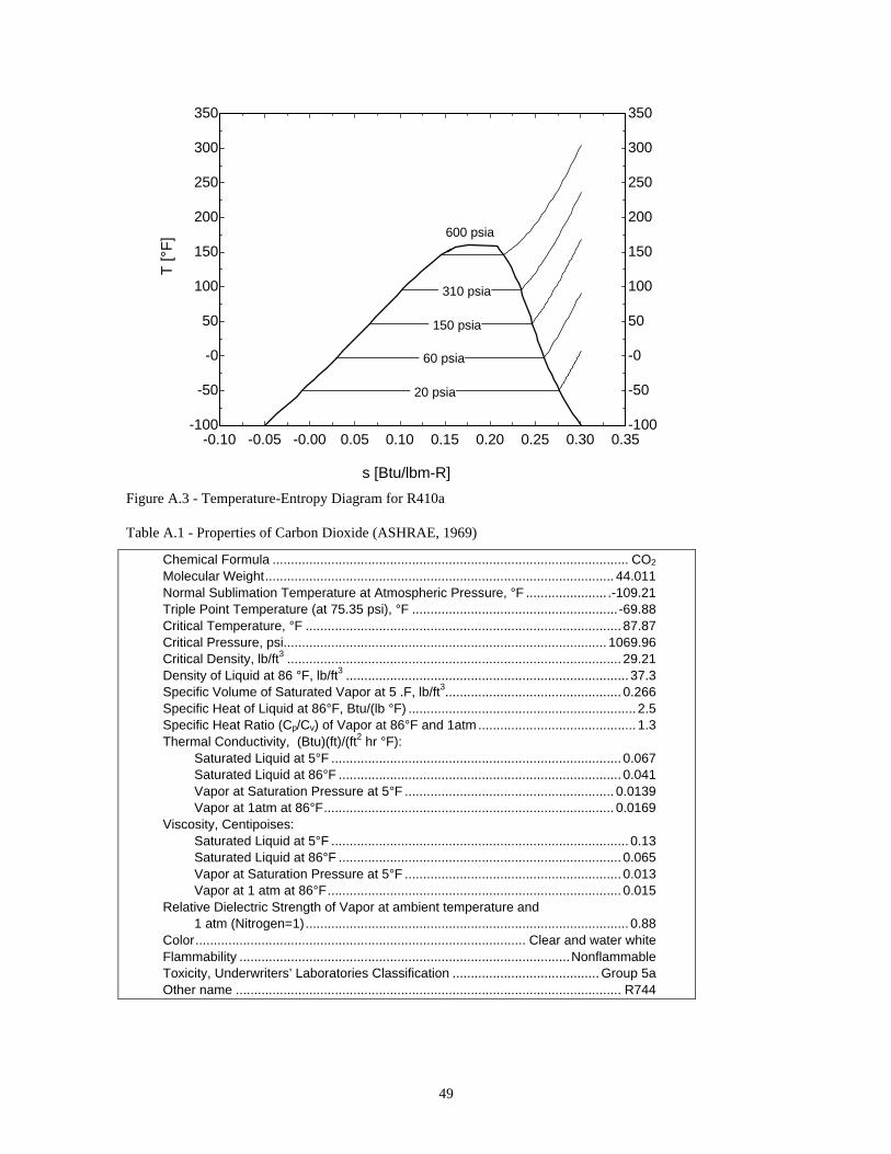
49

-0.10 -0.05 -0.00 0.05 0.10 0.15 0.20 0.25 0.30 0.35-100

-50

-0

50

100

150

200

250

300

350

-100

-50

-0

50

100

150

200

250

300

350

s [Btu/lbm-R]

T [°

F]

310 psia

150 psia

60 psia

20 psia

600 psia

Figure A.3 - Temperature-Entropy Diagram for R410a

Table A.1 - Properties of Carbon Dioxide (ASHRAE, 1969)

Chemical Formula ................................................................................................. CO2 Molecular Weight............................................................................................... 44.011 Normal Sublimation Temperature at Atmospheric Pressure, °F ...................... .-109.21 Triple Point Temperature (at 75.35 psi), °F ........................................................-69.88 Critical Temperature, °F ...................................................................................... 87.87 Critical Pressure, psi........................................................................................ 1069.96 Critical Density, lb/ft3 ........................................................................................... 29.21 Density of Liquid at 86 °F, lb/ft3 ............................................................................. 37.3 Specific Volume of Saturated Vapor at 5 .F, lb/ft3................................................ 0.266 Specific Heat of Liquid at 86°F, Btu/(lb °F) .............................................................. 2.5 Specific Heat Ratio (Cp/Cv) of Vapor at 86°F and 1atm........................................... 1.3 Thermal Conductivity, (Btu)(ft)/(ft2 hr °F): Saturated Liquid at 5°F ............................................................................... 0.067 Saturated Liquid at 86°F ............................................................................. 0.041 Vapor at Saturation Pressure at 5°F ......................................................... 0.0139 Vapor at 1atm at 86°F............................................................................... 0.0169 Viscosity, Centipoises: Saturated Liquid at 5°F ................................................................................. 0.13 Saturated Liquid at 86°F ............................................................................. 0.065 Vapor at Saturation Pressure at 5°F ........................................................... 0.013 Vapor at 1 atm at 86°F................................................................................ 0.015 Relative Dielectric Strength of Vapor at ambient temperature and 1 atm (Nitrogen=1)........................................................................................ 0.88 Color .......................................................................................... Clear and water white Flammability ..........................................................................................Nonflammable Toxicity, Underwriters’ Laboratories Classification ........................................ Group 5a Other name ......................................................................................................... R744

50

Table A.2 - Properties of R12 (ASHRAE, 1969)

Chemical Formula ............................................................................................. CCl2F2

Molecular Weight............................................................................................... 120.93 Boiling Temperature at Atmospheric Pressure, °F ...............................................-21.6 Freezing Temperature at Atmospheric Pressure, °F .............................................-252 Critical Temperature, °F ...................................................................................... 233.6 Critical Pressure, psi............................................................................................... 597 Critical Density, lb/ft3 ........................................................................................... 34.84 Density of Liquid at 86 °F, lb/ft3 ........................................................................... 80.67 Specific Volume of Saturated Vapor at 5 .F, lb/ft3................................................ 1.458 Specific Heat of Liquid at 86°F, Btu/(lb °F) .......................................................... 0.235 Specific Heat Ratio (Cp/Cv) of Vapor at 86°F and 1atm....................................... 1.139 Thermal Conductivity, (Btu)(ft)/(ft2 hr °F): Saturated Liquid at 5°F ............................................................................... 0.052 Saturated Liquid at 86°F ............................................................................. 0.040 Vapor at Saturation Pressure at 5°F ......................................................... 0.0047 Vapor at 1atm at 86°F............................................................................... 0.0059 Viscosity, Centipoises: Saturated Liquid at 5°F ............................................................................... 0.335 Saturated Liquid at 86°F ............................................................................. 0.254 Vapor at Saturation Pressure at 5°F ......................................................... 0.0108 Vapor at 1 atm at 86°F.............................................................................. 0.0127 Relative Dielectric Strength of Vapor at ambient temperature and 1 atm (Nitrogen=1).......................................................................................... 2.4 Color .......................................................................................... Clear and water white Odor ...............................................................................................Faint ethereal odor Flammability ..........................................................................................Nonflammable Toxicity, Underwriters’ Laboratories Classification .......................................... Group 6 Other name ........................................................................... Dichlorodifluoromethane

MATERIAL SAFETY DATA SHEET

1. CHEMICAL PRODUCT AND COMPANY INFORMATION Product Trade Name: PARCO LUBRITE 2

HENKEL CORPORATION, PARKER AMCHEM

32100 Stephenson Highway

Madison Height, MI 48071

Telephone number: (810) 583-9300

Emergency Number: (800) 424-9300

2. COMPOSITIOM INFORMATION

Table A.3 - Composition Information for PARCO LUBRITE 2

COMPONENT PERCENT

Phosphoric Acid 1-10 Nitric Acid 1-10

Nickel Nitrate <1 Manganese Dihydrogen Phosphate 20-40

Documents

Tribological Studies on Scuffing Due to the Influence of