Embed Size (px)
Citation preview

1
Tryphena Ow, An Examination of the Market Timing Ability of Mutual Funds using
Quarterly Trades
ACKNOWLEDGEMENTS
The journey to complete my thesis was both trying and fulfilling, I would not have
made it this far without the love and support from my family, lecturers and friends.
First and foremost, I would like to express my immense gratitude to my supervisor,
Professor Dominic Gasbarro. His tireless guidance, constructive suggestions and advice had
inspired me to strive for the best. Without his inexhaustible patience and guidance, this thesis
would not have been possible to accomplish. Under his abounding guidance, I have also
acquired new skills and insights, not only in academic studies but vigour in life.
Next, this valuable opportunity I have today, I owe to Professor Andrew Taggart. I am
very grateful to be awarded the Vice Chancellor’s SG50 Honours Scholarship. This award
has granted me a valuable opportunity to further my education abroad.
In addition, I would like to sincerely thank Mr Stephen Klomp for his hospitality and
kind guidance during my stay in Perth. I would also like to thank my lecturers, Dr Amy
Huang, Miss Thanesvary Subraamanniam and Miss Michelle Gander for their patience and
guidance throughout my units.
Last but not least, to my cherished family, I am deeply thankful and appreciative of
their boundless love, unwavering support and encouragement throughout this journey.

2
Tryphena Ow, An Examination of the Market Timing Ability of Mutual Funds using
Quarterly Trades
ABSTRACT
Past research primarily focus on evaluating market timing abilities using the returns
and stockholdings of mutual funds. We examine the market timing abilities of fund managers
using the trade proportions of mutual funds. These are statistically significant trade
proportions that encompass beta, sentiment beta and momentum. Trade proportions provide
insights on the direction that the fund manager was pursuing. Market and systemic risk
indicators are important for our study as they reflect the overall performance of the market
and the economy. We compare between the values of these indicators and the values of our
statistically significant trade proportions to evaluate if these values are highly correlated
during various market cycles. Using correlation and regression analysis, we examine the
relation between the trade proportions (dependent variable), the market and systemic risk
indicators (independent variables). We have also taken into consideration of certain
conditions that might affect the adjustments of these trade proportions and conducted some
preliminary and robust tests. In general, we expect that prior to a bull (bear) market, fund
managers will adjust their portfolios towards positive (negative) trade proportions.
Furthermore, majority of past studies had evaluated market timing abilities only during
recession periods therefore our study period between 1991 and 2012 has incorporated both
recession and boom periods to avoid biasness in results. However, similar to previous
findings, these trade proportions did not demonstrate superior market timing abilities.
Although no significant market timing abilities were exhibited, momentum trade proportions
displayed the most significant correlation and regression results. We observed an inverse
relationship between the positive momentum trade proportions and the momentum index.
This is consistent with fund managers having pursued a contrarian strategy.
3
Tryphena Ow, An Examination of the Market Timing Ability of Mutual Funds using
Quarterly Trades
CONTENTS
ACKNOWLEGDEMENTS 1
ABSTRACT 2
CONTENTS 3-7
FIGURES 8
GRAPHS 9
TABLES 10
1 INTRODUCTION 13-18
1.1 Introduction 13-18
2 LITERATURE REVIEW 19-60
2.1 Introduction 19
2.2 Overview of Literature 19-21
2.3 Characteristics of Mutual Funds 21-22
2.4 Mutual Fund Performance- Market Timing 22-23
2.4.1 Timing using Convex Relationship between Fund Returns and
Market Returns
23-25
2.4.2 Stationary Beta versus Non-Stationary Beta in Bull and Bear Markets 25-34
2.4.3 Evaluating Market Timing Abilities simultaneously with Security
Section Abilities
34-37
2.4.4 Free from Beta Estimates 37-39
2.4.5 Portfolio Performance Measures without Benchmarks 39-41
2.4.6 Volatility Timing 41-42
2.4.7 Downside of Returns Chasing Behaviour 43-44
2.4.8 Persistence in Fund Performance 44-46
2.4.9 Business Cycles and Predictability Skills 46-47
2.4.10 Stockholdings versus Trades 47-53
2.4.10.1 Market Timing Abilities 48-51
2.4.10.2 Stock Selection Abilities 51-54
2.4.11 Downside of Risk Shifting Behaviour 54-55

4
Tryphena Ow, An Examination of the Market Timing Ability of Mutual Funds using
Quarterly Trades
2.4.12 Successful Market Timing Abilities 56-57
2.5 Overview of Contrarian Strategies 57-58
2.5.1 Identifying Contrarian Strategies in Mutual Fund Trades 59
2.6 Conclusion of Literature Review and Motivation of Present Study 59-60
3 METHODOLOGY 61-79
3.1 Introduction 61
3.2 Overview of Methodology 61-63
3.3 Data Description 63
3.3.1 Bull and Bear Markets 63-64
3.3.2 Recession and Boom Periods 64-66
3.3.3 Four States of Bull and Bear Markets 66-68
3.4 Trades 68
3.4.1 Identifying Market Timing Trades 68
3.4.1.1 Formula for Identifying Market Timing Trades 68-69
3.4.2 Identifying Sentiment Beta Timing Trades 69
3.4.3 Identifying Momentum (Contrarian) Trades 69-70
3.5 Importance of Indices 70-71
3.5.1 Description of Indices 72-74
3.5.1.1 The S&P 500 Index 72
3.5.1.2 The Baker & Wurgler’s Sentiment Index 72
3.5.1.3 The S&P 500 Momentum Index 73
3.5.1.4 The S&P 500 Quality Index 73
3.5.1.5 The S&P 500 Growth Index 73-74
3.5.1.6 The S&P 500 Low Volatility Index 74
3.5.1.7 The S&P 500 High Beta Index 74
3.5.2 Systemic Risk Measures 74-77
3.5.2.1 Brief Description of Systemic Risk Measures (19 Elements) 75-77
3.6 Sources of Data and Availability 78
5
Tryphena Ow, An Examination of the Market Timing Ability of Mutual Funds using
Quarterly Trades
3.7 Trades’ Correlation with Indices 78-79
3.8 Conclusion of Methodology 79
4 RESULTS AND DISCUSSION 80-133
4.1 Introduction 80
4.2 Overview of Results and Discussion 80-83
4.2.1 Market Indicators 81
4.2.2 Systemic Risk Indicators 81-82
4.2.3 Overview of Analysis (Schematic Diagram) 82-83
4.3 Fund Quarters, Significant Fund Quarters and Proportions 83-85
4.3.1 Descriptive Statistics of Significant Fund Quarters and Proportions 86-87
4.4 Descriptive Statistics of Market and Systemic Risk Indicators 87-91
4.4.1 Descriptive Statistics (In Months) 87-90
4.4.2 Descriptive Statistics (In Quarters) 90-91
4.5 Performance of Market Indicators 92-99
4.6 Correlation Testing 99
4.6.1 Correlation Testing between Market Indicators (Main Market
Indicators and Sub-Market Indicators)
100-102
4.6.2 Correlation Testing between Systemic Risk Indicators 102
4.6.2.1 Brief Description of the Selected Systemic Risk Indicators 102-107
4.7 Final Selection of Market and Systemic Risk Indicators 107-109
4.8 Correlation and Regression Analysis between Trade Proportions
(DV) and Indicators (IV)
109-111
4.9 Overall Test for Correlation and Regression Analysis 111-117
4.10 Preliminary Test 117-129
4.10.1 Market Beta Trade Proportions 118-121
4.10.1.1 Market Index 118-119
4.10.1.2 Market “Return” Indicator 119-121
4.10.2 Sentiment Beta Trade Proportions 121-124
4.10.2.1 Sentiment Index 121-122

6
Tryphena Ow, An Examination of the Market Timing Ability of Mutual Funds using
Quarterly Trades
4.10.2.2 Sentiment “Return” Indicator 122-124
4.10.3 Momentum Trade Proportions 125-128
4.10.3.1 Momentum Index 125-127
4.10.3.2 Momentum “Return” Indicator 127-129
4.11 Summary Table of Significant Results based on Overall Analysis
and Preliminary Tests
130
4.12 Conclusion of Results and Discussion 131-133
5 ROBUST TESTING 134-164
5.1 Introduction 134
5.2 Overview of Robust Testing 134-137
5.3 Beta Trade Proportions and the Market “Return” Indicator 137-140
5.3.1 Test (1): Magnitude of Change 137-138
5.3.2 Test (2): Changes in Standard Deviation 138-139
5.3.3 Test (3): Changes in Signs 139
5.3.4 Test (4): Persistence in Index 139-140
5.4 Beta Trade Proportions and the Market Index 142-143
5.4.2 Test (4): Persistence in Index 142
5.5 Sentiment Beta and the Sentiment “Return” Indicator 143-146
5.5.1 Test (3): Changes in Signs 143
5.5.2 Test (4): Persistence in Index 144
5.6 Sentiment Beta and the Sentiment Index 146-147
5.6.1 Test (3): Changes in Signs 145-146
5.6.2 Test (4): Persistence in Index 146
5.7 Momentum Trade Proportions and the Momentum “Return”
Indicator
148-149
5.7.1 Test (4): Persistence in Index 148
5.8 Momentum Trade Proportions and the Momentum Index 149-151
5.8.1 Test (4): Persistence in Index 149
5.9 Multiple Regression Analysis 151-160

7
Tryphena Ow, An Examination of the Market Timing Ability of Mutual Funds using
Quarterly Trades
5.9.1 Market Beta 151-54
5.9.1.1 Positive Market Beta Proportions with the Market “Return”
Indicator
151-153
5.9.1.2 Positive Market Beta Proportions with the Market Index 153-154
5.8.2 Sentiment Beta 154-157
5.9.2.1 Positive Sentiment Beta Proportions with the Sentiment “Return”
Indicator
154-156
5.9.2.2 Positive Sentiment Beta Proportions with the Sentiment Index
Indicator
156-157
5.9.3 Momentum Trades 157-160
5.9.3.1 Positive Momentum Proportions with the Momentum “Return”
Indicator
157-159
5.9.3.2 Positive Momentum Proportions with the Momentum Index 159-160
5.10 Summary Table of Significant Results based on Robust and
Multiple Regression Tests
161
5.11 Conclusion of Robust Testing 162-164
6 CONCLUSION 165-79
6.1 Introduction 165
6.2 Overview of Conclusion 165-167
6.3 Significant Research Findings 167-168
6.4 Limitations of the Research 168
6.6 Areas of Future Research 169-170
6.6 Summary of Study 170-171
REFERENCES 169-179

8
Tryphena Ow, An Examination of the Market Timing Ability of Mutual Funds using
Quarterly Trades
FIGURES
Figure 1.1: Schematic Diagram: Overview of Methodology 18
Figure 2.1: The Characteristic Line of a Fund that Outguess the Market (Treynor
and Mazuy, 1966)
23
Figure 3.1: Schematic Diagram: Overview of Methodology
62
Figure 4.1: Trades, Market Indicators and Systemic Risk Indicators
83
Figure 4.2: Final Selection of Indicators for Analysis
108
Figure 4.3: Statistically Significant Trades and their Respective Indicators
109
Figure 5.1: Types of Robust Test Conducted
136

9
Tryphena Ow, An Examination of the Market Timing Ability of Mutual Funds using
Quarterly Trades
GRAPHS
Graph 4.1: Price Fluctuations of the Market Index, June 1991 to September 2012 92
Graph 4.2: Price Fluctuations of Market “Return” Indicator, July 1991 to
September 2012 93
Graph 4.3: Changes in the Sentiment Index Values, June 1991 to March 2011 95
Graph 4.4: Changes in the Values of the Sentiment “Return” Indicator, July 1991
to March 2011 96
Graph 4.5: Changes in the Momentum Index Values, September 2006 to
September 2012 97
Graph 4.6: Changes in the Values of the Momentum “Return” Indicator, October
2006 to September 2012
98

10
Tryphena Ow, An Examination of the Market Timing Ability of Mutual Funds using
Quarterly Trades
TABLES
Table 3.1: Bull and Bear Market Durations throughout the Trading Period
between July 1991 and October 2012
63
Table 3.2: Recession and Boom Durations throughout the Trading Period
between July 1991 and October 2012
65
Table 3.3: Data Sources, Availability and Types of Data
78
Table 4.1: Trades- Number of Fund Quarters, Significant Fund Quarters and
Proportions
85
Table 4.2: Descriptive Statistics of Statistically Significant Fund Quarters and
Proportions
86-87
Table 4.3: Descriptive Statistics of Market and Systemic Risk Indicators
(Presented in Months)
89-90
Table 4.4: Descriptive Statistics of Market and Systemic Risk Indicators
(Presented in Quarters)
91
Table 4.5: Correlation of Market Indicators: 73 Monthly and 25 Quarterly
Observations, September 2006 – September 2012
101-102
Table 4.6: Correlation between Systemic Risk Indicators: 247 Monthly
Observations and 83 Quarterly Observations, June 1991 to
December 2011
104-105
Table 4.7: Significant (at 0.01 Level) Results of Positive and Negative
Correlations between the Selected Systemic Risk Indicators: 83
Quarterly Observations, June 1991 to December 2011
106-107
Table 4.8: Overall Correlation and Regression between Trade Proportions and
Indicators
115-117
Table 4.9: Individual Correlation and Regression Analysis between Market
Beta Trades (Proportions) and the Market Index – June 1991 to
September 2012
118-119
Table 4.10: Individual Correlation and Regression Analysis between Market
Beta Trades (Proportions) and the Market “Return” Indicator – July
1991 to September 2012
120-121
Table 4.11: Individual Correlation and Regression Analysis between Sentiment
Beta Trades (Proportions) and the Sentiment Index– June 1991 to
March 2011
122

11
Tryphena Ow, An Examination of the Market Timing Ability of Mutual Funds using
Quarterly Trades
Table 4.12: Individual Correlation and Regression Analysis between Sentiment
Beta Trades (Proportions) and the Sentiment “Return” Indicator–
July 1991 to March 2011
124
Table 4.13: Individual Correlation and Regression Analysis between
Momentum Trades (Proportions) and the Momentum Index –
September 2006 to September 2012
127
Table 4.14: Individual Correlation and Regression Analysis between
Momentum Trades (Proportions) and the Momentum “Return”
Indicator – October 2006 to September 2012
129
Table 4.15: Significant Results based on Overall Analysis and Preliminary Tests
130
Table 5.1: Number of Quarters in relation to Market “Returns”- July 1991 to
September 2012
138
Table 5.2: Empirical Rule for Normally Distributed Data
139
Table 5.3: Robust Testing between Proportions of Beta Trades based and the
Market “Return” Indicator
141
Table 5.4: Robust Testing between Proportions of Beta Trades and the Market
Index
143
Table 5.5: Robust Testing between Proportions of Sentiment Beta Trades and
the Sentiment “Return” Indicator
145-146
Table 5.6: Robust Testing between Proportions of Sentiment Beta Trades and
Sentiment Index
147
Table 5.7: Robust Testing between Proportions of Momentum Trades and the
Momentum “Return” Indicator
149
Table 5.8: Robust Testing between Proportions of Momentum Trades and the
Momentum Index
150
Table 5.9: Robust Testing for Proportions of Beta Trades with the Market
“Return” Indicator and 11 Systemic Risk Indicator
152-153
Table 5.10: Robust Testing for Proportions of Beta Trades with the Market
Index and 11 Systemic Risk Indicator
154
Table 5.11: Robust Testing for Proportions of Sentiment Beta Trades with the
Sentiment “Return” Indicator and 11 Systemic Risk Indicator
155-156

12
Tryphena Ow, An Examination of the Market Timing Ability of Mutual Funds using
Quarterly Trades
Table 5.12: Robust Testing for Proportions of Sentiment Beta Trades with the
Sentiment Index and 11 Systemic Risk Indicator
157
Table 5.13: Robust Testing for Proportions of Momentum Trades with the
Momentum “Return” Indicator and 11 Systemic Risk Indicator
158-159
Table 5.14: Robust Testing for Proportions of Momentum Trades with the
Sentiment Index and 11 Systemic Risk Indicator
160
Table 5.15: Significant Results based on Robust and Multiple Regression Tests
161

13
Tryphena Ow, An Examination of the Market Timing Ability of Mutual Funds using
Quarterly Trades
CHAPTER 1
INTRODUCTION
1.1 Introduction
The performance measures for market timing abilities of fund managers has been a
predominant topic. Market timing is the ability of fund managers to tilt their portfolios in
accordance to the anticipated market trends to exploit returns. Common market trends are the
bullish and bearish markets. During bullish markets, fund managers can take advantage of the
market by buying high beta stocks and selling low beta stocks. In contrast, during bearish
markets, fund managers can take advantage of the market by buying low beta stocks and
selling high beta stocks.
In relation to predictability skills, fund managers can monitor the performance of the
market with the assistance of market indicators as they reflect the market movements. If the
index level of the S&P 500 market index consistently increases (decreases), we can anticipate
a bullish (bearish) market. However, market timing can also be a form of risk as the cost of
adjusting a portfolio may not be justified for the gains in return. Furthermore, portfolio tiling
may not necessarily suggest that fund managers are taking advantage of fluctuating
investment opportunities but a signal of ill motivated trades from mediocre abilities of fund
managers or agency issues (Huang, Sialm and Zhang, 2011). There is also a possibility of
mistiming which exposes funds to underperformance by selling (buying) stocks with high
(low) betas before a bullish (bearish) market period.
Early studies identified market timing abilities by evaluating the returns of mutual
funds. Treynor and Mazuy (1966) studied the returns of mutual funds on their historical
success of forecasting variations in the stock market. They reported that the fund returns and
the market returns had a convex relationship. Successful market timers would increase their

14
Tryphena Ow, An Examination of the Market Timing Ability of Mutual Funds using
Quarterly Trades
exposure to the market during bullish markets and decrease their exposure during bearish
markets. However, they did not consider how the systematic risk which is measured by beta
could vary in bullish and bearish markets. Subsequently, researchers incorporated the use of a
non-stationarity beta to evaluate market timing abilities of fund managers (Fabozzi and
Francis, 1979; Kim and Zumwalt, 1979; Miller and Gressis, 1980; Chen, 1982). A non-
stationary beta gives allowance for the increase in risk exposure. However, there were still no
significant evidence of market timing abilities.
Attention has been shifted to the evaluation of the performance of stockholdings and
trades to examine the predictive abilities of fund managers. Jiang, Yao and Yu (2007) found
positive market timing abilities when quarterly portfolio holdings were applied to a single
index model. However, Elton Gruber and Blake (2012) re-examined their study and argued
that using quarterly portfolio holdings may have resulted in an inaccurate conclusion of
market timing abilities as a vast number of trades were not captured in their analysis. In
addition, when monthly portfolio holdings were applied to a two index model, market timing
abilities were non-existence.
Comparing the use between stockholdings and trades, Chen, Jegadeesh and Wermers
(2000) reported that active stock trades represents a stronger opinion of a manager as
compared to a “passive” stockholding. Although no evidence of predictive abilities, Chen,
Jegadeesh and Wermers (2000) and Baker, Litov, Wachter and Wurgler (2010) found that
trade buys outperformed the trades they sell.
Using a different approach, researchers have also evaluated market timing abilities
simultaneously with stock selection abilities. Similar studies by Chang and Lewellen (1984)
and Chen and Stockum (1986) evaluated market timing and stock selection skills at the same
time using mutual fund returns. Chang and Lewellen (1984) proposed that there is a
15
Tryphena Ow, An Examination of the Market Timing Ability of Mutual Funds using
Quarterly Trades
possibility that fund managers might exploit returns by engaging in effective “macro” market
timing activities as well as careful “micro” security selection efforts. However, there were no
evidence of market timing abilities. Following the same method, Kacperczyk, Niewerburgh
and Veldkamp (2014) also evaluated market timing and stock selection abilities
simultaneously. However they took into consideration of the changing economic trends like
the boom and recession periods. They conditioned the state of the economy and developed a
new method where more weightage is given to a fund manager’s market timing success
during recession periods and stock picking success during boom periods. Studying mutual
fund holdings, they found market timing abilities in both recession and boom periods.
We contribute to the literature in several ways. First, we examine the market timing
abilities of fund managers by evaluating their statistically significant trade proportions that
encompass beta, sentiment beta and momentum. Second, we investigate if fund manager
adjust their portfolios between positive and negative trade proportions in accordance to the
various market cycles. Unlike past researchers, we study the proportions of these trades as
they provide insights on the direction that a fund manager was pursuing. We expect a higher
proportion of positive trades when the market is bullish or in an expansion phase. In contrast,
we expect a higher proportion of negative trades when the market is bearish or undergoing a
recession period. Third, we show that although momentum trade proportions had the least
number of quarter observations, they exhibited the most significant results from our
correlation and regression analyses. We observed that positive momentum trade proportions
exhibited an inverse relationship with the momentum index during bullish market periods.
Although results were inconsistent to our expectations, an inverse relationship suggests that
the fund manager may have pursed a contrarian strategy.
To identify trades that are engaged in market timing in any calendar quarter, we
conducted correlation and regression analyses between the trade proportions and their related

16
Tryphena Ow, An Examination of the Market Timing Ability of Mutual Funds using
Quarterly Trades
market indicators. We apply these measures to mutual fund trade proportions from 1991 to
2012. We conduct an overall correlation and regression test between the trade proportions
and their respective indicators to appreciate the general direction of their relationship. Next,
we consider how bullish and bearish markets will affect the adjustments of trade proportions.
We expect that during bullish market periods, the positive trade proportions would exhibit a
direct relationship with the market indicators. Similarly, during bearish market periods, we
expect negative trade proportions to exhibit a direct relationship with the market indicators.
Finally, various robust tests were also conducted to investigate if fund managers were
selective with the adjustments of their portfolio proportions based on market persistence,
turning points of the market and we study how big and small changes in the market returns
will affect their portfolio adjustment decisions.
We observe the following results from the correlation and regression analyses. Based
on the results of overall correlation and regression analysis, we observe that the positive
sentiment and positive momentum trade proportions exhibited significant results. However,
both trade proportions had an inverse relationship with their respective indicators. There were
no significant results from the beta trade proportions. Second, when bullish and bearish
market conditions are considered, the most number of significant results were exhibited from
the sentiment and momentum trade proportions. We observe an inverse relationship between
these trade proportions and their respective indicators. Third, based on the results from the
robust tests, the most number of significant results were also from the sentiment and
momentum trade proportions. Likewise, inverse relationships were exhibited between these
trade proportions and their respective indicators. Overall, despite momentum trade
proportions having the least number of quarter observations, they displayed the most number
of significant relationships. It is plausible that these fund managers have adopted a contrarian
strategy. Similar to previous findings, there we no evidence of market timing abilities.

17
Tryphena Ow, An Examination of the Market Timing Ability of Mutual Funds using
Quarterly Trades
We consider some limitations of the study. Although the use of quarterly data
observations provides more time allowance for fund managers to form market expectations
and make right decisions in portfolio adjustments, these observations may not be able to
capture sufficient information of fund managers with higher trading frequencies. It is also
possible that the total number of quarter observations might have affected our results.
Therefore, we suggest some areas of future research. We consider evaluating a longer time
period that incorporates all four recession periods in future studies as research have shown
that predictability skills are best displayed during recession periods. We also suggest
evaluating market timing and stock selection skills simultaneously with regards to the
changes in the economic conditions using the trade proportions of mutual funds.
This paper is organized in the following manner. In Section 2.0, we discuss the
literature review. In Section 3.0, we discuss the data and provide an overview of the
methodology. In Section 4.0, we discuss and present our findings. In Section 5.0, we conduct
various robust tests. In Section 6.0, we conclude our study. An overview of our study’s
methodology is provided (Refer to Figure 1.1).

18
Tryphena Ow, An Examination of the Market Timing Ability of Mutual Funds using
Quarterly Trades
Figure 1.1 Schematic Diagram: Overview of Methodology
The figure below illustrates the overview of our methodology. Trade betas that encompass beta,
sentiment beta and momentum are provided by Cullen et al. (2015). Quarterly data observations of
trade proportions are used for the analysis.
Indices
Trade Betas
(Proportions)
(1991-2012)
Trades associated with
Market Beta
Trades associated with
Sentiment Beta
Trades associated with
Momentum
S&P500 Market Index
Baker & Wurgler’s Sentiment Index
S&P 500 Momentum Index
S&P 500 Quality Index
S&P 500 Growth Index
S&P 500 Low Volatility Index
S&P 500 High Beta Index
Systemic risk
measures
Market Trends
-Bull and Bear Markets
-Recession and Boom Periods
-Further break down of Bull and Bear Markets
with the consideration of Volatility
Quarterly
Convert Data
Correlated
Check with
Daily
Monthly
Quarterly

19
Tryphena Ow, An Examination of the Market Timing Ability of Mutual Funds using
Quarterly Trades
CHAPTER 2
LITERATURE REVIEW
2.1 Introduction
This chapter describes the background and presents the literature review for this
study. In section 2.2, we discuss the background of our study and review the literature on the
key areas which are the market timing abilities of mutual funds managers, the evolution
performance measures which involves the use of stationarity and non-stationarity beta and the
examination of stockholdings and trades of mutual funds. We also identify the purpose of our
research and provide an overview of our methodology. Our sample comprises mainly of
statistically significant trade betas that encompass beta, sentiment beta and momentum of US
equity mutual funds over the period 1991 to 2012 and the data are provided by Cullen et al.
(2015).
2.2 Overview of Literature
Millions of people have invested in a once obscure financial instrument, the mutual
fund. Investors have constantly compared the advantages between active trading and passive
trading strategies of mutual funds. Over the years, the evaluation of mutual fund
performance has been vital to ensure optimal investment allocation as well as the
development of a mutual fund manager’s reward structure. Nevertheless, performance
measures have been consistently challenged and subsequently refined. Measures of a mutual
fund’s performance includes stock selection, market and industry timing abilities. Stock
selection and market timing abilities are the most popular measures of performance where
stock selection is the ability to select undervalued securities and market timing is the ability
to adjust security holdings to anticipate the movements of the market.

20
Tryphena Ow, An Examination of the Market Timing Ability of Mutual Funds using
Quarterly Trades
Determining the market timing abilities of mutual fund managers have been the focal
point of research. Managers with market timing abilities can attempt to exploit returns using
two common strategies. They can either move in and out of the market or conduct a tactical
asset allocation between low and high beta stocks using predictive methods by monitoring the
performance of indicators like the S&P 500 Market Index to detect any changes in the market
trends. The early stages of determining market timing abilities was derived using a quadratic
term in the capital asset pricing model (CAPM). Subsequently, researchers had focused on
the stationarity and non-stationarity of beta in the bull and bear market. The increase
(decrease) of a non-stationarity fund’s beta allows the fund’s equity holdings to rebalance in
the anticipation of the expected bull (bear) market.
In order to avoid these benchmark issues, recent studies have concentrated on mutual
fund holdings and mutual fund trades. The intuition is that a fund with successful market
timing skills will hold more stocks that possess high beta in bull markets and conversely hold
predominately lower beta in bear markets. Similarly, a fund will purchase high beta stocks
and sell low beta stocks when the market is expected to rise and purchase low beta stocks and
sell high beta stocks when the market is expected to fall.
We contribute to the literature in several ways. First, we examine market timing
abilities of fund managers by evaluating the statistically significant trades that encompass
beta, sentiment beta and momentum. Trade proportions are used as they provide insights on
the direction that the fund manager is pursuing. Second, we consider both upmarket and
downmarket periods in our study. Third, using a new approach, we investigate if fund
managers make technical adjustments to their portfolios according to different market trends
based on market indices. During the bullish periods, we expect a higher proportions of
positive trades in a fund’s portfolio. On the other hand, during bearish markets, we expect a
higher proportions of negative trades in a fund’s portfolio. Market timing is significant when
21
Tryphena Ow, An Examination of the Market Timing Ability of Mutual Funds using
Quarterly Trades
we observe a positive significant relationship between the market indices and the statistically
significant trade proportions.
This paper is organized in the following manner: in Section 2.0, we discuss the
literature of our research. Section 3.0, we provide and discuss the data and overview of the
methodology. In Section 4.0 we discuss the results of our research. Section 5.0, we conduct
various robust test. Finally in Section 5, we conclude the study and discuss about the
limitations of our study and suggest areas of future research.
2.3 Characteristics of Mutual Funds
Generally, in comparison to larger investment companies, individual investors lack of
substantial wealth to invest in large variety of stocks, bonds and securities. Consequently,
these individual investors turned into risk averse investors. Russell (2007) explained that
individual investors usually lack of professional knowledge and experience to make the best
decisions for their portfolios. Also, due to time management issues and complicated
paperwork, investors often struggle to keep up to their portfolios.
By offering diversification and simplicity for individual investors, mutual funds are a
good solution to these problems as they are a collection form of investments (Russell, 2007).
These funds are open-end investment companies and they pool funds of individual investors
offering them professional management by investing in a variety of securities or other assets
(Russell (2007); Bodie, Kane and Marcus (2014)). Instead of owning individual stocks or
bonds, mutual fund investors owns a portion of shares in a mutual fund and these shares
represent a portion of the holdings of the funds (Investopedia, 2016). The common types of
mutual funds are the money market funds, equity funds, bond funds, hedge funds and index
funds (Bodie, Kane and Marcus, 2014).

22
Tryphena Ow, An Examination of the Market Timing Ability of Mutual Funds using
Quarterly Trades
Commonly used by sophisticated investors due to their numerous advantages, mutual
funds are also well known for their professional management of money (Investopedia, 2016).
As investors may lack time or expertise to manage their own portfolio, these funds offer
convenience and cost efficiency as they allow investors to have an inexpensive way to make
and monitor their investments (Investopedia, 2016). Bodie, Kane and Marcus (2004)
explained that as mutual funds includes a wide range of securities, this reduces portfolio risk
as any loss in a particular security can be minimised by the gains of others (Investopedia,
2016).
Mutual funds also offer lower transaction costs as they are usually purchased and sold
in large volumes of securities in bulk (Bodie, Kane and Marcus, 2004). Compared to
individual investors, these large scale investors are usually given a discounted trading cost.
Additionally, mutual funds are valuable for their liquidity advantages. Although they are a
collective form of investments, they allow shares to be converted into cash at any point of
time of request like an individual stock (Bodie, Kane and Marcus, 2004).
2.4 Mutual Fund Performance – Market Timing
In our study, market timing is the ability of a fund manager to adjust his or her
portfolio composition between high volatile stock and low volatile stocks based on using
predictive methods such as technical indicators like the market index. The market index
reflects the overall performance of the market and suggesting periods of bullish or bearish
market trends.
Fund managers that possess market timing abilities can generate superior returns by
adjusting their portfolios in accordance to the anticipated market trend. During bullish
(bearish) market periods, fund manager can adjust their portfolios towards high (low) volatile

23
Tryphena Ow, An Examination of the Market Timing Ability of Mutual Funds using
Quarterly Trades
stocks. In other words, during bullish (bearish) periods, fund manager can exploit returns by
buying high (low) beta stocks and selling low (high) beta stocks.
2.4.1 Timing using Convex Relationship between Fund Returns and Market Returns
There has been an ongoing debate on the best performance measure for market timing
abilities of fund managers. Traditional performance measures like the Capital Asset Pricing
Model (CAPM) have reported that the relationship between the fund returns and market
returns are linear. Conversely, the study by Treynor and Mazuy (1966) showed that the
relationship between the fund returns and market returns are actually convex. Treynor and
Mazuy (1966) evaluated market timing abilities of mutual funds based on their historical
success in predicting major fluctuations in the stock market. They concluded that successful
market timers would increase their exposure to the market when a bullish period is
anticipated and reduce exposure to the market when a bearish period is anticipated. This
action causes the characteristic line of the portfolio to surpass the market as the portfolio
asset structure can be constantly adjusted (Figure 2.1).
Figure 2.1: The Characteristic Line of a Fund that Outguess the Market (Treynor and Mazuy,
1966)
Volatility
Volatility
Fund Returns
Market Returns
Characteristic Line

24
Tryphena Ow, An Examination of the Market Timing Ability of Mutual Funds using
Quarterly Trades
Using the basis of the CAPM, Eq. (1), Treynor and Mazuy (1966) developed a least
square regression technique performance focusing on the squared relation between fund
returns and market returns. A curvature line was identified by fitting in the characteristic line
data of 57 open-end mutual funds using their yearly data observations of returns during the
period between 1953 and 1963, Eq. (2):
𝑅𝑖𝑡 = 𝑅𝑓 + 𝛽𝑖(𝑅𝑚𝑡 − 𝑅𝑓𝑡) (1)
𝑅𝑖𝑡 − 𝑅𝑓𝑡 = 𝑎𝑖 + 𝛽𝑖(𝑅𝑚𝑡 − 𝑅𝑓𝑡) + 𝛾𝑖(𝑅𝑚 − 𝑅𝑓𝑡)2
+ ℯ𝑖𝑡 , (2)
where, 𝑅𝑖𝑡 denotes return on assets of the selected fund at time t, 𝑅𝑓𝑡 denotes risk free return
rate at time t, 𝑅𝑚𝑡 is the return on the market at time t, 𝑎𝑖 denotes a selectivity ability,
𝛾𝑖 denotes the parameter measuring the market timing performance, if 𝛾𝑖 > 0, it implies the
existence of a timing ability. The difference between the equation of the CAPM model and
the Treynor and Mazuy model is the addition of 𝛾𝑖(𝑅𝑚 − 𝑅𝑓𝑡)2 as this changes the linear
relationship between the fund returns and market returns into a quadratic equation.
Treynor and Mazuy used yearly data observations of returns as they believed that
even for smaller funds, the frequency of portfolio changes which will alter their fund’s
volatility will not happen more than once a year. However, only one out of 57 funds exhibited
a curve characteristic line. This suggest that on average, mutual funds were not successful at
outguessing the market. Treynor and Mazuy (1966) concluded that any excess returns
generated were not from the success of timing abilities but from the abilities of fund
managers in identifying under-priced industries and companies.
Supporting the study of Treynor and Mazuy (1966), Williamson (1972) stated that the
relationship between the fund returns and the market returns would be convex instead of
linear. Based on the characteristic line graph, when the line is curved upwards at the upper

25
Tryphena Ow, An Examination of the Market Timing Ability of Mutual Funds using
Quarterly Trades
right and lower left end, this suggest that mutual funds had performed well in bearish markets
and performed even better during bullish markets.
Williamson (1972) attempted to identify market timing abilities by reviewing the
available published data of 180 mutual funds during the period between 1961 and 1970.
However, similar to Treynor and Mazuy (1966), on average, no mutual funds were able to
outperform the market. Moreover, four out of 180 funds displayed significant unsuccessful
forecasting. Against expectations, these funds were more volatile during bearish market and
less volatile during bullish markets.
2.4.2 Stationary Beta versus Non-Stationary Beta in Bull and Bear Markets
Jensen (1968) believed that the performance of risky investment portfolios is the
ability of a portfolio manager to earn superior returns through successful predictions of future
security prices. These returns should be higher than the returns expected by the portfolio
manager for the level of risk associated with their portfolios. This belief is based on the
concept that on average, the riskier the asset is, the higher the returns will be. Portfolio
managers will be compensated for taking on additional risk. If the asset’s actual returns are
above the expected returns of the asset, a positive alpha is established.
On the contrary to earlier studies that evaluated forecasting abilities of portfolio
managers using relative performance measures, Jensen (1968) has provided an absolute
measure of performance. Absolute performance measure is a measure that is compared
against a certain standard. The Jensen’s equation determines the superior returns obtained
when deviated from the benchmark, Eq. (3):
𝛼𝑖 = [𝑒(𝑟𝑖𝑡) − 𝑟𝐹𝑡] − 𝛽𝑖(𝑒(𝑟𝑚𝑡) − 𝑟𝑓𝑡), (3)

26
Tryphena Ow, An Examination of the Market Timing Ability of Mutual Funds using
Quarterly Trades
where, 𝑟𝑖𝑡 denotes the return of fund 𝑖 at time t, 𝛼𝑖 denotes the abnormal returns of the fund
(an idea of forecasting abilities), 𝛽𝑖 denotes the systematic risk of the fund 𝑖, 𝑟𝑚𝑡 denotes the
return of the market at time t and 𝑟𝑓𝑡 denotes the risk free rate at time t. The value of alpha
could either positive or negative. Having a positive alpha would imply superior forecasting
abilities and in contrast, having a negative alpha would imply either poor selection choices or
the existence of high expenses.
Given that the predictability skills of a portfolio manager not only involves the skills
to predict price movements of individual securities and the general behaviour of future
security prices, the Jensen (1968) model also considers the abilities of a fund manager to
forecast the market behaviour. Henceforth, the Jensen (1968) model not only evaluates the
portfolio manager’s ability to predict how much a security or portfolio is expected to earn
given the level of systemic risk (measured by beta) but also measures the ability of a portfolio
manager to forecast the market’s behaviour. However, this is based on the assumption that
the portfolio manager tries to maintain the given level of risk in his or her portfolio.
Jensen (1968) investigated the existence of predictability skills by analysing 115 open
ended mutual funds using their yearly data observation of returns during the period between
1945 and 1964. Based on the results, on average, mutual funds were not able to predict
security prices to outguess the market henceforth underperforming buy and hold strategies.
They were also unsuccessful in their trading activities to recoup brokerage expenses. We
consider some limitations of this study. The assumption that the portfolio manager attempts
to maintain the same level of risk may have caused inaccurate results. As mutual funds are
being actively managed, it is reasonable to expect changes in the level of risk due to the
buying and selling decisions of portfolio managers.

27
Tryphena Ow, An Examination of the Market Timing Ability of Mutual Funds using
Quarterly Trades
Subsequently, there has been attention drawn to the stability of the systematic risk
measured by beta in bull and bear market conditions. The systematic risk of mutual funds in
different market conditions is an important factor in evaluating the market timing abilities of
a fund manager. If there is different beta for different market conditions, using a stationary
beta for the entire period can result in different conclusion of a fund manager’s abilities.
During market changes, when a stationary beta is used for the entire time period there is no
consideration for the additional risk exposure. If a fund manager correctly adjusts the fund’s
beta in an anticipation of a bull market, the beta in a bull market would be greater than the
estimation of beta for both bull and bear market period. One of the limitations from Jensen
(1968) study was the use a stationary beta for the entire period of the study as the fund
managers attempted to on average, maintain the given level of risk in their portfolio.
Taking into consideration a non-stationary beta, Fabozzi and Francis (1979)
investigated if the beta of mutual funds varies in bullish and bearish markets. A statistical
model was developed by Fabozzi and Francis (1979) to examine if the systemic risk of
mutual funds was altered during different market conditions. The monthly data observations
of returns of 85 mutual funds were tested between the period from 1965 and 1971. In order to
examine if the systematic risk (beta) are different in various market conditions, this equation
has taken into consideration of beta shifting, Eq. (3):
𝑅𝑖 = 𝐴1𝑖 + 𝐴2𝑖𝐷𝑡 + 𝛽1𝑖𝑅𝑚𝑡 + 𝛽2𝑖𝐷𝑡𝑅𝑚𝑡 + ℯ𝑖𝑡, (4)
where, 𝑅𝑖 denotes the excess returns of fund i, 𝑅𝑚𝑡 denotes the excess returns on the market
𝐷𝑡 denotes a dummy variable which is unity if the tth period is a bull market and zero
otherwise, The coefficients of the dummy variable, 𝐴2𝑖 and 𝐵2𝑖, measure the differential
effects of bull market conditions on the alpha, 𝐴1𝑖 and beta, 𝐵1𝑖 respectively and ℯ𝑖𝑡 is the

28
Tryphena Ow, An Examination of the Market Timing Ability of Mutual Funds using
Quarterly Trades
random error term. This equation allows the shifting of alpha and beta and is designed to
determine if the regression coefficients are significantly different in bull and bear markets.
Fabozzi and Francis (1979) reported that there were three definitions of bull and bear
markets for this study. First, defined by a well-established textbook (Cohen, Zingbarg and
Zeikel, 1973), certain months were designated as bull and bear markets in accordance to
market trends. Second, when market returns positive, the market is known to be bullish.
When market returns are negative, the market is known to be bearish. Third, without the
consideration of market trends, months with market returns higher (lower) than one half of
the standard deviation of market returns over the sample period are designated as bull (bear)
markets.
While betas of individual securities may be stable despite changes in market trends
like the bull and bear markets, Fabozzi and Francis (1979) argued that there is a possibility
for a non-stationary beta to occur even if the fund manager did not attempt to adjust the
portfolio risk. They considered how the individual securities’ betas may be intertemporally
unstable. Also, changes in the relative market value weights of individual securities will alter
the portfolio’s beta, which is the weighted average beta regardless if the betas of individual
securities were not altered. Therefore, a benchmark is created to determine if the number of
funds that shifted in beta were a result of a planned changed in risk exposure. For comparison
purpose, 85 random portfolios were created as benchmarks. Each stock of the 85 random
portfolios were given equal weightage.
Despite considering a non-stationary beta, results suggest that regardless of different
market conditions, on average, mutual funds did not respond differently. Similar to previous
studies, mutual fund managers were not able to outguess the market to earn higher risk-

29
Tryphena Ow, An Examination of the Market Timing Ability of Mutual Funds using
Quarterly Trades
adjusted returns for shareholders. Fund managers did not alter their fund’s beta to benefit
from the different market conditions.
Fabozzi and Francis (1979) revealed three reasons why fund managers were not
observed to increase their funds’ beta during bearish to bullish market periods or decrease
their funds’ beta during bullish to bearish periods. One, there were random beta coefficients
from a significant number of New York Stock Exchange (NYSE) stocks and the portfolio
managers might have overvalued or undervalued the beta. Two, there is a possibility that the
portfolio manager was unable to foresee changes in market conditions hence was unable to
shift the fund’s beta during bullish markets. Three, although fund managers may have
correctly anticipated the right change in direction of the market, the cost of altering a fund’s
beta may not be justifiable for the gains in return.
An extension to the Fabozzi and Francis (1979) study, Kim and Zumwalt (1979)
investigated if there were variations of returns of securities and portfolios in up (bull) and
down (bear) markets. This process has the effect of separating the total variation of the
security or portfolio returns into two components, variations when the market is up and
variations when the market is down. Kim and Zumwalt (1979) pointed out that although the
beta of mutual funds are not significantly different in up and down market periods, the
variations of returns of mutual funds may be different. If investors are presumed to be risk-
averse, they would expect to receive a premium for bearing additional risk from the “down”
market and expected to pay a premium for the returns they would receive from the “up”
market.
For the development of the study, two assumptions were employed. The first
assumption was that each security may react differently in up and down markets. If securities
do respond differently, beta coefficients may be determined for both up and down markets

30
Tryphena Ow, An Examination of the Market Timing Ability of Mutual Funds using
Quarterly Trades
and investigated for statistically significant differences. There were three measures to
determine what establishes an “up” or “down” market. An “up” market are months with rate
of returns on the market portfolios that exceed the 1) average market return, 2) the risk free
rate or 3) zero. Otherwise, the market is defined as a “down” market. The single index model
was modified to examine both up and down betas, Eq. (5):
𝑅𝑖𝑡 =∝𝑖+ 𝛽𝑖+𝑅𝑚𝑡
+ + 𝛽𝑖−𝑅𝑚𝑡
− + ℯ𝑖𝑡, (5)
where, 𝑅𝑖𝑡 denotes the excess return of fund i , ∝𝑖 denotes the actual return of fund i minus
the expected return of fund i, 𝑅𝑚𝑡 denotes the excess return on the market, ℯ𝑖𝑡 is the random
error term, 𝛽𝑖+is determined from the months when the returns comes from the “up” market
and 𝛽𝑖− is determined when the returns come from the “down” market. As the number of
securities in the portfolio increases, the unsystematic risk also known as firm-specific risk
would be diversified away. The variance of portfolio equation would be written as, Eq. (6):
𝜎𝑝2 = (𝛽𝑝
+)2𝜎𝑝2
𝑝+ + (𝛽𝑝−)2𝜎𝑝
2𝑝− , (6)
where, 𝜎𝑝2 is the variance of the portfolio. The formula is separated into (𝛽𝑝
+)2𝜎𝑝2
𝑝+ being the
variations from the bull market and (𝛽𝑝−)2𝜎𝑝
2𝑝− being the variations from the bear market.
The second assumption was that investors had a preference for greater up side
variation of returns and a preference for a smaller downside variation of returns. This
suggests that an investor has a preference that is positively related to the upside variations
and negatively related to the downside variations. Kim and Zumwalt (1979) believed that
investors require a risk premium on the downside portion of variation and a negative risk
premium on the upside portion of the variation. Expressed in Eq. (7):
𝐸(𝑅𝑝) = 𝑅𝑓 + 𝜆1 𝛽𝑝+ + 𝜆2 𝛽𝑝
− (7)

31
Tryphena Ow, An Examination of the Market Timing Ability of Mutual Funds using
Quarterly Trades
where, 𝜆1 𝛽𝑝+ denotes the negative coefficient and 𝜆2 𝛽𝑝
− denotes the positive coefficient. The
two beta model of equation 7 was tested to determine if the expected negative value for 𝜆1
and positive value for 𝜆2 was confirmed.
Kim and Zumwalt (1979) developed the two beta model to incorporate the responses
of beta during “up” and “down” market periods. The variations of returns in both market
periods were investigated using the monthly data observations of returns from a sample of
322 securities between the periods from 1962 to 1976. This model allows the separation of
the total systemic risk into two components, risk from upside variations markets which are
considered to be favourable and risk from bearish markets which are considered to be
unfavourable.
Results reflected that out of 322 securities, 34 exhibited significantly different up and
down market betas. In comparison to the Fabozzi and Francis (1979) study, more securities
displayed statistically significant differences between “up” market and “down” market betas
than would occur randomly. The signs of the regression coefficients were also correct and
statistically significant, suggesting that investors do receive a risk premium for tolerating
downside risk. Consistent to Kim and Zumwalt’s expectations, the negative premium was
associated to the beta of the “up” market. This suggests that the measurement of downside
variation of returns is more appropriate when measured by the “down” market beta rather
than the conventional single beta in the market model.
Miller and Gressis (1980) created a new measure based on the traditional CAPM
which allows and statistically estimates the extent of non-stationarity in the relationships
between the fund returns and market returns. This measure allows a precise estimation of
alpha and beta in the presence of non-stationarity beta. Miller and Gressis (1980) revealed
that if non-stationarity is significant in a risk return relationship but is ignored, this can result

32
Tryphena Ow, An Examination of the Market Timing Ability of Mutual Funds using
Quarterly Trades
in misleading information as the estimates of alphas and betas are calculated based on a
stationary beta which is the weighted averages of the actual values. When mutual funds are
actively managed, the level of systemic risk would fluctuate as a result of the buying and
selling decisions of their managers. Hence beta, the measure of systematic risk should not be
ignored as this might result in biased results. It is also reasonable to expect non-stationary
risk return relationships in some mutual funds as well-managed funds would take advantage
of the market by altering their betas in accordance to the general market movements.
Miller and Gressis’s (1980) approach is based on the traditional CAPM which allows
and statistically gauge the extent of non-stationarity in relationships between the returns of
funds and the returns from the market. In order to obtain a more precise estimate of beta and
alpha, time can be segmented into intervals during which the betas are stationary. A
partitioning algorithm and partition selection procedure is conducted on the sample of 28
mutual funds using the weekly data observations of returns between the periods from 1973 to
1974. Unlike previous researchers that evaluated the performance of mutual funds using
yearly or monthly data observations of returns (Jensen, 1986; Fabozzi and Francis, 1979;
Kim and Zumwalt, 1979), Miller and Gressis (1980) used weekly data observations of returns
as they believed that it is a more appropriate measure in detecting shifts between the risk and
returns of mutual funds.
The presence of a non-stationary beta would suggest either changes in the distribution
of risk in the economy or changes in the mutual fund portfolio composition. Investors are
interested in such changes as they attempt to take advantage of these deviations to earn
superior returns. Based on the results, only one out of 28 funds exhibited stationary betas and
the rest had betas that varied over the periods. Based on correlation and regression analysis
results of the information gathered from the partition regression, a mixture of results were
exhibited between the betas and the market returns. There were some evidence of weak

33
Tryphena Ow, An Examination of the Market Timing Ability of Mutual Funds using
Quarterly Trades
positive relationships and some weak negative relationships between the betas and market
returns. Similarly, there were also weak negative relationships and weak positive
relationships between the alphas and betas. However, there were no statistically significant
relationships of either type.
Following up on the studies that incorporated the use of non-stationary beta, Chen
(1982) re-examined the relationship between the risk and returns of mutual funds in in bull
and bear market conditions. Chen (1982) evaluates the study of Kim and Zumwalt (1979) as
their procedure of valuing “up” and “down” market betas may have led to in inaccurate
results in the risk analysis of “up” and “down” markets.
Chen (1982) revealed that the study by Kim and Zumwalt (1979) gave inconsistent
results due to multicollinearity issues which resulted in large sampling variances of estimates
of the “up” and “down” market betas. Also, the model did not take into consideration that the
beta coefficient would change over time. Chen (1982) used a time-varying beta coefficient
approach to resolve these issues. It is revealed that the two beta model used for the test of the
trade-off between the risk and returns in “up” and “down” market is constant regardless of a
stable or non-stable beta coefficient. The two beta model from the Kim and Zumwalt’s study
was modified to be, Eq. (8):
𝐸(𝑅𝑝𝑡) = 𝑅𝑓 + 𝛽𝑝+𝐸(𝑅𝑚𝑡 − 𝑅𝑓)
++ 𝛽𝑝
−𝐸(𝑅𝑚𝑡 − 𝑅𝑓)−
+ ℯ𝑖𝑡 (8)
where, 𝐸(𝑅𝑝𝑡) denotes the expected return of the portfolio, 𝑅𝑓 denotes the risk free rate of
interest, 𝛽𝑝+ denotes the bull market beta, 𝛽𝑝
− denotes the bear market beta and ℯ𝑖𝑡 denotes the
random error term.
The sample of 360 mutual funds’ monthly data observations of returns were tested
between the periods from 1965 to 1977. Similar to Kim and Zumwalt’s (1979) results, Chen

34
Tryphena Ow, An Examination of the Market Timing Ability of Mutual Funds using
Quarterly Trades
(1982) concluded that investors do require a premium for taking on risk from the downside
market and investors pay a premium for the returns they receive from the “up” market. The
results of the time varying beta approach method have supported the Kim and Zumwalt’s
findings that the breakdown of total systemic risk into risk due to upside deviation of returns
and risk due to the response of a bear market still appeared to be correct even with a non-
stationary beta. Irrespective of a stationary or non-stationary beta, investors do request
compensation for undertaking the risk from the variation of returns from the bear market
which was viewed as unfavourable and pay a premium for the upside variation of returns
which was viewed as favourable.
Both studies by Chen (1982) and Kim and Zumwalt (1979) revealed that an
appropriate measure of downside risk (bear market) would be the “down” market beta instead
of a stationary beta. It is not appropriate to consider the use of a stationary beta as a
measurement of the market as the market cycle changes over time. A stationary beta does not
give any allowance for the increase in risk exposure.
2.4.3 Evaluating Market Timing Abilities simultaneously with Security Selection
Abilities
Past research have investigated the market timing abilities of fund managers
individually. Using a different approach, Chang and Lewellen (1984) evaluated market
timing abilities of fund managers simultaneously with security selection abilities. They
believed that portfolio managers might be able to exploit returns by engaging in effective
“macro” market timing activities as well as cautious “micro” security selection efforts. That
is the ability to modify the total risk composition of their portfolios in the anticipation of the
general movements of the market. This study considers the fact that a non-stationary beta
would be a more appropriate measure of mutual fund performance. Based on the studies by
35
Tryphena Ow, An Examination of the Market Timing Ability of Mutual Funds using
Quarterly Trades
Fabozzi and Francis (1979), Kim and Zumwalt (1979), Miller and Gressis (1980) and Chen
(1982), they found some evidence that mutual fund portfolios do not have a constant risk
position over time. They also concluded that skills of market timing may well be a
measurement of a fund manager’s decision process.
Chang and Lewellen (1984) conducted a parametric statistical procedure that allowed
a joint test for the presence of either security selection or superior market timing skills in
managed portfolio to investigate the performance of 67 mutual funds using their monthly data
observations of returns between the periods from 1971 to 1979. Majority of research have
evaluated the performance of mutual funds based on the single market model equation, Eq.
(9):
𝑍𝑝(𝑡) − 𝑅(𝑡) = 𝑎𝑝 + 𝛽𝑝[𝑍𝑚(𝑡) − 𝑅(𝑡)] + 𝜖(𝑡), (9)
where, 𝑍𝑝(𝑡) denotes the observed rate of return on the portfolio p during the period, 𝑅(𝑡)
denotes the simultaneous rate of return on a riskless asset, 𝑍𝑚(𝑡) denotes the return on the
fully diversified “market” portfolio of all risky assets during t and 𝜖(𝑡) denotes the random
error term with it being a value of 0. 𝛽𝑝 is assumed to be stationary over time. When alpha
has a positive value, this indicates superior return performance based on security selection
efforts. However, this model only evaluates stock selection abilities and does not take into
consideration that the level of systemic risk (𝛽𝑝) might change over time.
The equation was later modified by Henriksson and Merton (1981) to a least square
regression which evaluates the stock selectivity and market timing abilities of mutual fund
abilities separately. It was also modified to capture an “up-market beta” and a “down-market
beta.” The modified equation was, Eq. (10):
𝑍𝑝(𝑡) − 𝑅(𝑡) = 𝛼∗ + 𝛽1∗𝑋1(𝑡) + 𝛽2
∗𝑋2(𝑡) + 𝜖𝑝∗ (𝑡), (10)
36
Tryphena Ow, An Examination of the Market Timing Ability of Mutual Funds using
Quarterly Trades
where, 𝑋1(𝑡) and 𝑋2(𝑡) =𝑍𝑚(𝑡) − 𝑅(𝑡), 𝛽1∗ denotes the “up-market beta” of a managed
portfolio and 𝛽2∗ denotes the “down market beta”. The contributions of returns have been
separated into two components, α represents the returns due to security selection ability and
𝛽 is used to measure the portfolio’s market-timing skill. When there is no existence of market
timing abilities, the value of beta would be zero.
While this was a joint test that considered both market timing and stock selection
abilities of fund managers, results suggest that on average, neither skilful market timing nor
clever security selection abilities were evident. Overall, mutual funds were unable to outguess
the market. It seemed that passive strategies still have an upper hand in mutual fund
investments.
Similar to Chang and Lewellen (1984), Chen and Stockum (986) also investigated the
market timing and stock selection abilities of fund managers simultaneously. Traditional
performance measures like the Sharpe ratio assumed that that the systematic risk level of a
fund is a fixed coefficient rather than a decision variable. However, this results in inaccurate
performance measures as the risk of the portfolio varies over time. Following which, studies
have incorporated the use of a non-stationary beta. However, they did not consider that the
mutual fund’s beta could also be non-stationary when fund managers are not engaged in
timing decisions (Fabozzi and Francis, 1979; Kim and Zumwalt, 1979; Miller and Gressis,
1980; Chen, 1982). Hence, the presence of a non-stationary beta does not necessary represent
the existence of market timing abilities.
Chen and Stockum (1986) presented a generalized varying parameter model to
examine the performance of mutual funds by allowing for both timing decisions of funds and
random behaviour of fund’s systematic risk levels. Although the generalized varying

37
Tryphena Ow, An Examination of the Market Timing Ability of Mutual Funds using
Quarterly Trades
parameter model is similar to the Treynor and Mazuy model, this model allows the beta of
mutual funds to be a decision variable instead of a fixed coefficient, Eq. (11):
𝑅𝑖𝑡 = 𝑎𝑖 + 𝑅𝑚𝛽− + 𝜆𝑖𝑅𝑚𝑖
2 + 𝜔𝑖𝑡 (11)
where, 𝜔𝑖𝑡 equals (𝜇𝑖𝑡 + 𝜖𝑖𝑡𝑅𝑚𝑡). 𝑅𝑖𝑡 denotes mutual fund i’s return at time t, 𝑅𝑚 denotes the
market return at time t, 𝜇𝑖𝑡 denotes random shock, β denotes target systemic risk, 𝑎𝑖 measures
the selectivity component and 𝜆𝑖𝑅𝑚𝑖2 measures changes due to market timing. A portfolio
beta might still be non-stationary even if fund managers are not actively managing their
portfolios by adjusting the portfolio beta in accordance to the market. This is because a
portfolio beta might respond differently to various market cycles.
Chen and Stockum (1986) examined 43 mutual funds using their quarterly data
observations of returns between the periods from 1975 to 1982. Unlike prior studies that used
monthly or yearly data observations of returns, Chen and Stockum (1986) stated that the use
of quarterly data observations gives fund managers an extended period of time to form
market expectations and adjust their portfolios accordingly. Throughout this sample period,
there were two bull and two bear market periods. By incorporating both cycles of the
markets, it will help to reduce biasness in this study.
Based on the results, 30% of funds showed selectivity, 19% were random betas and
14% showed significant but negative market timing performance. Although there were some
significant selectivity abilities, results suggest that similar to previous findings, mutual funds
did not reflect any market timing abilities regardless individually or as a group.
2.4.4 Free from Beta Estimates
On the contrary to prior research, Ferri, Oberhelman and Roenfeldt (1984) examined
the market timing abilities of mutual funds without the use of beta estimates. This method

38
Tryphena Ow, An Examination of the Market Timing Ability of Mutual Funds using
Quarterly Trades
focuses on the composition of assets in a fund’s portfolio and investigates alterations in the
composition prior to variations in the broad level of stock market prices. The main objective
of this method is to examine whether a fund manager’s decision to gradually increase or
decrease the fund’s commitment to common stocks. The expectations of fund managers are
reflected on the decisions that they made and simultaneously shifts the portfolio’s market-
related volatility.
A fund manager is successful at market timing when their decisions and expectations
are consistent with the later movements of the market. For instance, a fund manager who
anticipates a bearish market will lower the portfolio’s volatility by decreasing the percentage
of assets in a portfolio that are invested in stocks. Market timing skills are exhibited if the
later market is bearish. Likewise, successful market timing is exhibited when a fund manager
increases the portfolio assets invested in stocks in the expectations of an increase in market
prices and the later market is bullish.
Ferri, Oberhelman and Roenfeldt (1984) examined the quarterly changes in the
mutual fund’s stock holdings of 69 mutual funds between the periods from 1975 to 1980.
These types of mutual funds have aggressive management with a preference of being
completely invested by stocks. Therefore, any alterations in these funds are considered as an
attempt to forecast or time the market movements. Additionally, two subgroups of
stockholdings were also examined, those preceding extensive fluctuations in stock prices and
those when managerial reallocations of portfolios are not impacted by shareholder’s
contributions or withdrawal from funds.
Market timing abilities are evaluated by examining the increases and decreases in a
fund’s relative commitment to stocks measured by the ratio of net purchases or sales of
common stocks (NETPS) to total assets. If the NETPS has a positive value, the fund has
39
Tryphena Ow, An Examination of the Market Timing Ability of Mutual Funds using
Quarterly Trades
purchased more stock than it sold, increasing its exposure to market risk. A t test was
conducted to compare the mean levels of NETPS for a fund quarter before an increase in the
stock index with the mean NETPS for the fund quarter before a decrease in the stock index.
Ferri, Oberhelman and Roenfeldt (1984) hypothesized that the NETPS is classified as an
upmarket decision if the stock index increases during the subsequent months and the NETPS
is classified as downmarket decision if the stock index decreases during the subsequent
months. The null hypothesis is rejected if the average NETPS for the upmarket is
significantly larger than the average NETPS for the down market. However, the test of means
could be inaccurate as there is a possibility that a fund made merely a few large mistakes as
the test results are reliant on the extent of the deviations in stock holdings. Therefore, a
frequency test is also conducted as it only examines the direction of changes in stock
holdings prior to the movements in the stock index and eliminates the limitations of the test
of means. A correct decision can either be classified as a positive NETPS before a bullish
market or a negative NETPS before a bearish market.
Based on the results, although a few funds displayed some market timing abilities, on
average, there were no significant market timing abilities exhibited. In sum, although this
study offers an alternative way of examining market timing abilities which is a method that is
free from the estimates of beta, there were no new evidence that fund managers possess
market timing abilities.
2.4.5 Portfolio Performance Measures without Benchmarks
Past researchers have evaluated performance measures of mutual funds by comparing
the returns of managed portfolios to the returns of a benchmark portfolio. However, this
could be a bias measure of market timing abilities as results are dependent on the choice of
benchmark selected. Often, information regarding the portfolio composition of funds are not

40
Tryphena Ow, An Examination of the Market Timing Ability of Mutual Funds using
Quarterly Trades
utilised. Grinblatt and Titman (1993) believed that by making use of information about the
portfolio composition, the method of comparing returns to a benchmark portfolio can be
eliminated.
This method is adapted by the Event Study Measure where the performance of mutual
funds are evaluated by calculating the differences between the returns of assets during the
portfolio period known as “the event period” and returns of a later date known as “the
comparison period”. This is the belief that the assets held in a well-managed portfolio (event
period) would have higher returns compared to periods when assets are not included in any
portfolios (comparison period). This method uses later period returns compared to earlier
period returns as they have taken into account that some portfolio managers are likely to pick
their assets based on their past returns. However, this might be a bias assumption as it forces
the researcher to ignore assets that lacked returns in the comparison periods.
Grinblatt and Titman (1993) developed a new measure that is not subjected to
survivorship biases. It is based on the assumption that from the standpoint of uninformed
investors, the direction of expected asset returns is constant over time. This implies that the
portfolio holdings of an uninformed investor does not have any form of relationship with the
future returns. Unlike a well-informed manager who is able to predict when certain assets
will exhibit higher or lower than average returns, the direction of the expected asset returns
will vary over time. The manager can take advantage of these changing expected returns by
tilting his or her portfolio weights towards assets that have increased in expected returns and
tilt away from assets that have decreased in expected returns.
Grinblatt and Titman (1993) examined 155 mutual funds quarterly changes in
stockholdings from the period between 1974 and 1984. Concluding results showed that on
average, mutual fund portfolios exhibited positive abnormal investment performances and
41
Tryphena Ow, An Examination of the Market Timing Ability of Mutual Funds using
Quarterly Trades
that the strongest performance was computed from the aggressive growth category of funds
which earned significantly positive risk adjusted returns. In relation to the study by Ferri,
Oberhelman and Roenfeldt (1984), any movements in these funds are considered as an
attempt to forecast or time the market movements. Although no market timing abilities were
present, this article emphasized that superior performance can be predicted without the use of
a benchmark when portfolio holdings were examined.
2.4.6 Volatility Timing
Previous studies have examined the market timing abilities of mutual fund managers
exclusively by comparing the returns between their funds and the market (Treynor and
Mazuy, 1966; Jensen, 1968; Fabozzi and Francis, 1979; Kim and Zumwalt, 1979; Miller and
Gressis, 1980; Chen, 1982). The main theory behind these studies often investigate if fund
managers have taken advantage of superior information by adjusting their funds towards
more (less) volatile stocks in the anticipation of bull (bear).
Often, fund managers encounter difficulties in predicting market returns. Using a new
perspective, Busse (1999) investigated the funds’ ability to time market volatility. He
examined if funds change market exposure in relation to market volatility changes and
highlighted that volatility timing is a significant influence in the returns of mutual funds as it
leads to higher risk-adjusted returns.
Attention has been shifted to market volatility for two reason. First, unlike market
returns which are hard to predict, market volatility is predictable because it is persistent. High
volatility is usually followed by high volatility and low volatility is usually followed by low
volatility. Second, majority of performance measures are risk adjusted. These measures affect
the cash flows of funds and how funds manage risk has repercussions for manager
compensation. However, it is uncertain that a fund manager can increase risk adjusted

42
Tryphena Ow, An Examination of the Market Timing Ability of Mutual Funds using
Quarterly Trades
performance or investor utility by timing market volatility. Therefore, Busse (1999)
investigates if funds respond to changes in market volatility and how these strategies will
affect the performance of funds.
Busse (1999) motivated volatility timing in the perspective of a fund manager,
assuming that fund managers attempt to time market exposure in the best interest of the fund
shareholder. Busse (1999) analysed the daily data observation of returns of 230 domestic
equity funds between 1985 and 1995 with a daily single factor volatility timing model to
study how managers respond to publicly available information. This single factor volatility
timing model is modified from the four index model by adding in terms to capture the effects
of volatility timing. Unlike previous researchers that analysed monthly return data (Fabozzi
and Francis, 1979, Kim and Zumwalt, 1979; Chen 1982; Chang and Lewellen, 1984), the use
of daily returns’ data allows a more efficient estimate of time variations in systematic risk
considering that monthly returns’ data might not be able to capture the day to day activities of
active mutual funds.
A conditional analysis was conducted to provide detailed explanations of mutual fund
risk and the reasons for its changes. It also allows the evaluator to differentiate between
passive effects and the effects by public information usage. Furthermore, it also helps to
differentiate among active managers of different abilities and as such lead to better asset
allocation decisions.
Based on the results, Busse (1999) found a strong inverse relationship between the
funds’ systemic risk levels and conditional market volatility. When conditional market
volatility is higher than average, systemic risk levels are lower. When conditional market
volatility is high, funds that reduce systemic risk earned higher risk-adjusted returns. This
demonstrates that mutual funds have taken advantage of the superior information by

43
Tryphena Ow, An Examination of the Market Timing Ability of Mutual Funds using
Quarterly Trades
increasing their market exposure when there is low market volatility and decreasing their
market exposure when market volatility is high.
2.4.7 Downside of Returns Chasing Behaviour
Over the years, researchers have focused on exploiting mutual fund returns. A
contrasting article by Karceski (2002) developed an agency model to express that such return
chasing behaviour of fund managers will lead to beta being under-priced to the degree that is
predicted by the standard CAPM. Based on Karceski’s (2002) model, he revealed that the
goals of fund managers and the behaviour of return chasing fund managers will influence
fund management to adjust their portfolios towards high beta stocks. Based on the theory of
supply and demand, this will lead to a high demand of high beta stocks which lead to an
increase in prices and in turn lower the expected returns. The model is supported by three
verifiable facts. First, investors tend to buy funds that have recently displayed extraordinary
returns. Second, fund managers chase returns through time. During the transition period from
the bear to the bull market, there is a tendency of larger cash inflows into the equity mutual
fund industry. Third, during bullish market periods, high beta stocks outperforms low beta
stocks.
Karceski (2002) believed that active fund managers focus on outperforming peers
during the transition phase between bearish and bullish markets as returns are usually larger.
The rewards from the bullish market are usually higher than the rewards from the bearish
market as cash inflows are usually minimised after a “down” market. Mutual fund investors
would tilt their portfolios towards high beta stocks during an upward market in anticipation
that it will lead to a larger cash inflow as high beta stocks typically outperform in bull
markets. However, this return chasing behaviour by mutual fund managers will lead to

44
Tryphena Ow, An Examination of the Market Timing Ability of Mutual Funds using
Quarterly Trades
CAPM’s beta to be either under-priced or overpriced than the expected amount, resulting in a
reduction of beta risk premium in equilibrium. In an equilibrium world, the demand for high
beta stocks prior the bull market will push their price higher and expected returns lower.
Karceski (2002)’s model predict that these actions will cause expected returns to fall.
The model investigates the monthly holdings of mutual funds from the period between 1984
and 1996. Consistent to Karceski (2002) expectations, results reflected that fund investors
appeared to be inexperienced as they tend to increase their equity funds stake after the market
goes up and pick funds based on their past performance despite justified warnings by
disclaimers to the contrary. Based on the agency model created, the behaviour of mutual fund
managers chasing returns across funds cause them to tilt towards high beta stocks resulting in
a flatter security market line and as a result reduces the expected returns premium for high
beta stocks. The total stock portfolio was over weighted with aggressive growth funds (high
beta stocks) compared to income equity funds (low beta stocks).
Results reflected that equity mutual funds held a larger percentage of high beta stocks
compared to the overall equity market portfolio. Karceski (2002) predictions were right that
due to active fund managers tilting towards high beta stocks, this reduces the expected return
premium for high beta stocks and flattens the security market line. In some extreme cases,
this may lead to the returns of low beta stocks surpassing the equilibrium expected returns of
high beta stocks despite conventional risk measures such as beta or standard deviation and
performance in bear markets suggesting that high beta stocks should acquire a higher
expected return.
2.4.8 Persistence in Fund Performance
Bollen and Busse (2005) believed that superior information is built on the expectation
that some fund managers possess significant predictive abilities and if this ability persists, it

45
Tryphena Ow, An Examination of the Market Timing Ability of Mutual Funds using
Quarterly Trades
allows vigilant investors to predict future performance based on past results. Bollen and
Busse (2005) examined the persistence in mutual fund performance emphasizing on short
term periods.
There are two types of decision making strategies, stock selection and market timing.
Stock selection refers to predicting returns of individual stocks and market timing refers to
predicting relative returns of broad asset classes. Majority of past studies found no significant
evidence that fund managers were able to achieve abnormal returns over long periods
regardless pursuing a stock selection or market timing strategies.
Bollen and Busse (2005) examined if mutual fund performance persist over a
relatively short period of three months. They reported that fund performance exists for a
relatively short amount of time due to the mutual fund industry being competitive by nature
or to managerial turnover. Having short measurement periods provides a more accurate way
of identifying top performers. Daily fund returns are examined with quarterly measurement
periods as Bollen and Busse (2005) argued that monthly fund returns will not be an efficient
estimation. Previous studies that used mostly monthly data of returns found insignificant
evidence that fund managers were able to generate positive abnormal returns from stock
selection abilities or market timing abilities over a long period of time. Also, using quarterly
measurement periods controls for cash flows as it allows mutual fund factor loadings to
gradually alter.
The parameters of stock selection and market timing models were estimated and stock
selection and market timing abilities were examined using the four factor model and two
timing models. Bollen and Busse (2005) allowed the coexistence of both types of abilities in
their measurement as previous studies have focus on either one of this abilities individually
without taking into consideration that some fund managers are stock pickers whereas some

46
Tryphena Ow, An Examination of the Market Timing Ability of Mutual Funds using
Quarterly Trades
are market timers. By stereotyping them as one type of fund manager could result in
inaccurate results. There is a likelihood that fund managers may also switch strategies. They
studied the daily returns of 230 funds between 1985 and 1995. Funds are ranked every
quarter by their risk adjusted return measured over a three month period using market timing,
stock selection and mixed strategy models. Following which, the risk adjusted return of
deciles of funds over the subsequent three month period are measured.
While abnormal returns were reflected in the top decile of funds suggesting
persistence in mutual fund performance, Bollen and Busse (2005) argued that abnormal
returns cease to exist when funds are being evaluated over a longer time horizon. This reflects
that superior performance is short lived and only significant when they are evaluated
regularly. Taking into consideration of account transaction cost and taxes, superior returns
may be generated by passive strategies like the buy and hold strategy compared to a
performance chasing strategies even if short term performance is foreseeable.
2.4.9 Business Cycles and Predictability Skills
Avramov and Wermers (2006) reported that most investment profits are generated
from the predictability in manager skills. Based on prior research, most studies find that
passive strategies have consistently outperformed active strategies. However, an article
focusing on stock picking skills reported that active management achieved significant returns
when examined during recession periods in comparison to expansion periods (Moskowitz,
2000). This suggests that business cycle variables may be advantageous in identifying
actively managed mutual funds that outperform.
Avramov and Wermers (2006) designed optimal portfolios of no load, open-end US
domestic equity mutual funds in the presence of manager selectivity and benchmark timing
skills, mutual fund risk loadings and benchmark returns. They analysed both ex post out of

47
Tryphena Ow, An Examination of the Market Timing Ability of Mutual Funds using
Quarterly Trades
sample performance and ex ante investment opportunity set delivered by predictability based
strategies. When an investor does not have any predictability skills, he or she will invest in
index funds. In comparison, investors that believed in the possibility of predicting fund risk
loadings and benchmark returns will invest in actively managed funds.
Avramov and Wermers (2006) analysed the optimal portfolio of 1301 open-end, no
load US domestic equity mutual funds which include index funds, sector funds, actively
managed funds and exchange traded funds. These mutual funds’ monthly database was over
the sample period between 1975 and 2002. Results reflected that incorporating predictability
skills makes actively managed funds more attractive and these funds generated larger Sharpe
ratios. Out of sample optimal portfolios that did not incorporate any predictability skills
produced negative alphas. By incorporating manager’s skills in predictability into long term
strategies, these strategies had outperformed their Fama-French and momentum benchmarks
by 2% to 4% per year by timing industries over business cycle and additional 3% to 6% per
year by choosing funds that outperform the industry benchmarks.
Avramov and Wermers (2006) found that predictability in manager skills are the
leading basis of investment profitability. Active management adds significant values in their
investment and industries are important in locating outperforming mutual fund. Also,
investment strategies that incorporated predictability manager selectivity and benchmark
timing skills consistently outperform. Predictability skill strategies performed best during
recessions but are also good during expansion. These skills are able to identify the best
performing funds during both expansion and recessions. Overall, active management of
mutual funds adds on significant values.
2.4.10 Stockholdings versus Trades
48
Tryphena Ow, An Examination of the Market Timing Ability of Mutual Funds using
Quarterly Trades
Numerous of studies have concluded that on average, mutual funds are not able to
outguess the market. Actively managed funds have underperformed their benchmark
portfolios. Although there has been no significant evidence of successful fund possessing
market timing or stock selection abilities to surpass the market, investors have continued to
invest in actively managed funds in hopes of achieving abnormal returns. Articles have
shifted their attention on evaluating the performance of stockholdings and trades of mutual
funds. Majority of these studies have focused on evaluating stock selection abilities with the
use of stockholdings and trades. Regardless, we examine how stockholdings and trades will
result in different values of active trading strategies.
2.4.10.1 Market Timing Abilities
Early studies have evaluated the returns of mutual funds but find no significant
evidence of market timing abilities. Jiang, Yao and Yu (2007) reported that these return-
based test are exposed to “artificial timing” biasness. They proposed an alternative market
timing measurement using mutual fund holdings to investigate the active changes of fund
betas as these holdings are not subjected to artificial timing biasness.
Using holdings, Jiang, Yao and Yu (2007) estimated the beta of a fund as the
weighted average of the individual stocks’ betas from the portfolio holdings and directly
tested if the covariance between the fund betas at the initial holding period and the market
returns of the holding period is significant. In comparison to return based measures that relied
on ex post realised returns to estimate the adjustments of beta, these measurements based on
holdings used only ex ante information. Therefore, these measures do not suffer from any
biasness by subsequent trading activities in the course of a holding period or dynamic trading
effect. In addition these holding based measures have better statistical power.
49
Tryphena Ow, An Examination of the Market Timing Ability of Mutual Funds using
Quarterly Trades
Jiang, Yao and Yu (2007) evaluated 2,294 actively managed equity mutual funds by
applying both return-based test and holdings-based test from the period between 1980 and
2002 using a single index model. Monthly observation data of returns of mutual funds are
used for the return based test and quarterly holdings of mutual funds are used for the holdings
based test. Jiang, Yao and Yu (2007) reflected that the results from the return based measures
exhibited similar results from majority of the research that on average, mutual funds have
slightly negative but insignificant market timing abilities. Whereas the results reflected from
holdings based measure suggested that on average, mutual funds have positive timing
abilities.
Implementing the alternative market timing measurement, Jiang, Yao and Yu (2007)
conducted the holding based test using active changes of fund beta and results suggested that
mutual funds time the market through active trading. While linking several fund
characteristics and market timing performances, they discovered market timing funds are
typically funds with high industry concentration, particularly those with a tilt towards small
cap stocks and with large fund size. Additionally, they stated that fund managers adjust fund
betas in accordance to macroeconomic variables such as price to earnings ratios and total
dividend yield. When macroeconomic variables are controlled, average market timing
abilities still appeared to be positive. This suggest that fund managers are not only utilising
information from the publicly accessible macroeconomic information but also private
information to time the market.
Following up on the study by Jiang, Yao and Yu (2007), Elton, Gruber and Blake
(2012) re-examined the existence of market timing abilities with the use of monthly portfolio
holdings instead of quarterly portfolio holdings. Elton, Gruber and Blake (2012) believed that
the use of monthly holdings data will capture a vast number of trades that are missed by
quarterly holdings data and provide a better estimation of timing trades. Unlike, Jiang, Yao

50
Tryphena Ow, An Examination of the Market Timing Ability of Mutual Funds using
Quarterly Trades
and Yu that only investigated the market timing abilities of actively traded equities, Elton,
Gruber and Blake (2012) investigated a full range of securities like options, futures, preferred
stock, bonds and non-traded equity. They reported that these range of securities use
additional instruments to time and ignoring their presence will result in inaccurate results of
market timing decisions.
In the study by Jiang, Yao and Yu (2007) which found positive market timing
abilities, they estimated portfolio betas with the use of portfolio holdings and security betas
and investigated the effects of changing betas with a single index model. Elton, Gruber and
Blake (2012) investigated if similar results will be exhibited when a multi index model is
used. The multi index model recognises bonds as an individual vehicle for timing.
Furthermore, they also re-examined market timing abilities with the used the Fama-French
model both with unconditional and conditional betas and a model that studies the effect of
adjusting allocation across industries.
Elton, Gruber and Blake (2012) examined the monthly data of holdings between the
periods from 1994 to 2005. Based on the results, negative timing abilities were reflected.
Results from the Fama-French model suggest that timing decisions of fund managers led to a
decrease in performance regardless being measured using conditional or unconditional
sensitivities. Similarly, the sector allocation’s model also reflected negative timing measures.
Inconsistent to the results from the single index model, the results from the two index
model reflected a different conclusion. Elton, Gruber and Blake (2012) discovered that the
timing decisions of mutual funds did not result in superior returns. First, when the managers
change their exposure to the market, they do so by adjusting their exposure to small stocks or
higher growth stocks. Taking into account of this shifting procedure, timing results was
altered as such unlike the single index model which reflected positive timing abilities, the two

51
Tryphena Ow, An Examination of the Market Timing Ability of Mutual Funds using
Quarterly Trades
index model exhibited negative timing abilities. Second, Elton, Gruber and Blake (2012)
reported that a large number of trades have been neglected with the use of quarterly holdings.
Third, the use of a wider range of securities may have impacted the results and that the major
contribution of negative timing abilities were from high technology stocks. Although no
market timing abilities were exhibited, Elton, Gruber and Blake (2012) showed that with
monthly holdings, timing ability can be measured more precisely as compared to using
quarterly or yearly data which misses a large number of trades.
While Jiang, Yao and Yu (2007) concluded that positive timing abilities are
significant, the study by Elton, Gruber and Blake (2012) questioned the credibility of their
results. Jiang, Yao and Yu (2007) assumes that the beta on the market of all securities that are
not traded equity is zero, as a result non-traded equity, bonds, futures, options, preferred
stocks and mutual funds are treated as identical instruments with each of them having a beta
on the market of zero. Elton, Gruber and Blake (2012) reported that 18.5% of trades by an
average fund manager were not captured when market timing measures were applied to
quarterly data holdings. In addition, even though Jiang, Yao and Yu (2007) found market
timing abilities using a single-index model, these findings did not hold up when a two-index
model was used.
2.4.10.2 Stock Selection Abilities
Chen, Jegadeesh and Wermers (2000) studied the value of active mutual fund
management by evaluating the stockholdings and trades of mutual funds. By examining both
stockholdings and trades, it resolves the issue of whether a stock truly signifies superior
information in regards to the stock’s value. They presumed that active stock trades represents
a stronger opinion of a manager in comparison to a passive decision of holding an existing
position in a stock as stockholdings may be prompted by reasons in relation to non-

52
Tryphena Ow, An Examination of the Market Timing Ability of Mutual Funds using
Quarterly Trades
performance like transaction costs and capital gain taxes. Therefore, they expect any evidence
of stock selection abilities to exhibit from the examination of trades compared to holdings.
Chen, Jegadeesh and Wermers (2000) compared the returns from stock holdings and
trades by high turnover funds and the returns from stock holdings and trades by low turnover
funds of 2,424 mutual funds quarterly data from the period between 1975 and 1995 to study
the value of active mutual fund management.
Based on the results from the examination of stock holdings, Chen, Jegadeesh and
Wermers (2000) found no difference in the performance of stocks that are most widely held
by mutual funds and those that are least widely held. However, when examining mutual fund
trades, stocks buys significantly gave higher returns than stocks sold. They concluded that
examining trades would be a better choice for portfolio performance examining trades as it is
a more powerful metric to determine the existence of superior information.
Pinnuck (2003) examined the performance of Australian fund managers’ monthly
stock holdings as well as trades of mutual funds to investigate if they possess superior
information. Stockholdings allow a more accurate examination of performance as compared
to traditional performance measures that relied on the examination of mutual funds’ return.
The examination of mutual funds’ trades is motivated by the study of Chen, Jegadeesh and
Wermers (2000) as the study showed that trades of mutual funds are more likely to represent
a signal of private information compared to passive stockholdings.
Pinnuck (2003) evaluated the stockholdings and trades of 35 Australian active equity
fund managers using their monthly portfolio holdings data from the period between 1990 and
1997. Unlike previous studies that examine the performance of stocks held at calendar quarter
ends, Pinnuck (2003) examined month end portfolios as they argued that quarter end
portfolios may not fully represent a typical fund portfolio and in addition have reporting

53
Tryphena Ow, An Examination of the Market Timing Ability of Mutual Funds using
Quarterly Trades
biases. Taking into consideration of the study by Chen, Jegadeesh and Wermers (2000) which
argued that studying trades of mutual funds would be a more powerful metric to determine
the existence of superior information. Pinnuck (2003) also investigated on the performance of
the stocks a fund manager trades, specifically stocks buys and stocks sold.
Based on the results, stocks held by fund managers on average, realised abnormal
returns. The results from the evaluation of individual trades showed that stocks that are
purchased by fund managers achieve abnormal returns but stocks sold did not exhibit any
abnormal returns. This suggests that fund managers do not possess superior information with
regards to bad news.
Pinnuck (2003) concluded that overall fund managers have the ability to select stocks
that realised positive abnormal returns. However, there were some limitations of this study.
Due to a limited time period, results may be time period specific. Also due to a small sample
size, results may be sample specific too. Trades exhibiting abnormal returns may result from
the consequences of price pressure rather than fundamental information. Survivorship
biasness which is the tendency for mutual funds with poor performance to be dropped by
mutual fund managers may have some impact on the resulted abnormal returns.
Baker, Litov, Wachter and Wurgler (2010) developed an alternative method of
identifying trading skills. They studied the nature of stock picking abilities and constructed
measures of trading skills built on how stocks are traded and held by fund managers perform
at subsequent corporate earnings announcement. It is the ability to buy stocks that are about
to enjoy high returns prior to their upcoming quarterly earnings announcements and sell
stocks prior to the suffering of low returns upon that announcement. This method enables a
more powerful approach to detect skilled trading and attempts to differentiate between the
winners from losers based on their trading activities. They believed that this approach will be

54
Tryphena Ow, An Examination of the Market Timing Ability of Mutual Funds using
Quarterly Trades
more useful in detecting trading skills as it exploits segments of the returns at earning
announcements.
Baker et al. (2010) analysed the returns by fund holdings but focused mainly on the
trades of the funds measure mutual fund manager trading skills by using the sample of
quarterly data from several million funds from the period between 1980 and 2005. Results
show that the average fund buys performs better at future earnings announcements than
control stocks and that the fund sells perform worse. Mutual fund trades also forecasted
earnings surprises and this concludes that mutual fund managers are able to trade profitably
as they are able to predict earnings-related fundamentals. In sum, mutual fund trades have the
ability to forecast earnings fundamentals.
2.4.11 Downside of Risk Shifting Behaviour
Majority of the research focus on the benefits of risk shifting but Huang, Sialm and
Zhang (2011) aimed to fill the gaps of the performance consequences of risk shifting
behaviour. They reported that mutual funds alter their risk levels significantly over time and
that this risk shifting behaviour may be a result of ill motivated trades of unskilled or agency-
prone fund managers who trade for personal benefits to increase their personal compensation.
However, risk shifting can also be executed when a skilled fund manager trades to take
advantage of their stock selection and timing abilities.
Huang el at. (2011) investigated the performance consequences of risk shifting and
examined what stimulates this risk shifting behaviour. They reported that altering the risk
levels of mutual funds may not be harmful to investors for two reasons. First, as mutual funds
have the incentive to shift risk to take advantage of the competition for extra returns,
investors are not necessarily hurt by risk shifting. Second, risk shifting behaviour shows
one’s superior skill since it is associated to the activeness of the investment tactics of funds.

55
Tryphena Ow, An Examination of the Market Timing Ability of Mutual Funds using
Quarterly Trades
When active managers change their portfolio composition to take advantage of their stock
selection or timing abilities this will result in a change of risk exposure as an unintentional
consequence. However if risk shifting funds indeed excel better than other funds, then this
risk shifting behaviour profits the investors.
When risk shifting is motivated by agency related issues, superior performance of
funds would not be expected. Likewise, fund managers lacking of skills and abilities are more
likely to alter risk levels and therefore worst performance of funds would be expected.
However, if risk shifting is executed by a skilled managers taking advantage of their market
or stock selection abilities, superior performance from funds are expected.
In order to investigate the risk shifting behaviour of mutual funds, Huang el at. (2011)
used the quarterly holdings of the sample of 2,979 equity funds over the period between 1980
and 2009. They measured the risk shifting behaviour of mutual funds by proposing a holdings
based measure to investigate the difference between the volatility of a fund’s current holdings
and its past realised volatility.
Results exhibited that funds that change risk tend to subsequently perform worse than
funds that maintained a stable risk level. Huang et al. (2011) described three reasons for risk
shifting. First, funds can alter risk levels by switching between equity holdings and cash
holdings. Second, based on equity holdings, fund managers can alter risk by changing their
exposure to systematic risk. Fund managers can switch between high beta stocks and low
beta stocks. Third, funds can alter risk by changing their exposure to certain industries or by
deviating from their benchmarks. Based on these reasons, Huang et al. (2011) reported that
inferior performance of funds are mostly caused by fund increasing idiosyncratic risk
exposure whereas funds that alter their risk between equity and cash holdings and between
systematic risk levels did not exhibit much reductions in fund performance. In addition, risk

56
Tryphena Ow, An Examination of the Market Timing Ability of Mutual Funds using
Quarterly Trades
shifting can be costly for active mutual funds. Therefore, risk shifting does not necessarily
apply that skilled fund managers are taking advantage of changing investment opportunities.
Instead, risk shifting is more likely to be a signal of ill motivated trades either from inferior
ability of fund managers or agency issues.
2.4.12 Successful Market Timing Abilities
Kacperczyk, Nieuwerburgh and Veldkamp (2014) examined fund manager skills and
developed measures of market timing and stock picking. Similar to Chang and Lewellen
(1984) and Chen and Stockum (1986), they evaluated both market timing and stock selection
abilities simultaneously. Kacperczyk et al. (2014) proposed a new definition of fund
manager’s skill as the rational ability to pick stocks or time the market.
Past researchers find little market timing evidence as it is typically exhibited only in
recession periods. Therefore, unlike previous studies that isolate stock picking and market
timing abilities unconditional to the state of the economy, Kacperczyk et al. (2014) evaluated
market timing and stock selection abilities with regards to the changing of economic
conditions, taking into consideration for both booms and recession periods. They consider the
fact that the type of skills a fund manager exhibits might alter in accordance to the state of the
business cycles.
By conditioning the state of the economy, Kacperczyk et al. (2014) found surprising
results that managers have performed in both stock picking and market timing abilities. Those
who are stock picking during boom periods are also good at market timing during recessions.
Therefore, Kacperczyk et al. (2014) developed a new real time measure to detect a fund
manager’s skill where more weightage is given to a fund manager’s market timing success
during recession period and stock picking success during bloom period. This new measure
demonstrates persistence of up to one year and forecasts performance.
57
Tryphena Ow, An Examination of the Market Timing Ability of Mutual Funds using
Quarterly Trades
In order to determine the skills of fund managers, Kacperczyk et al. (2014)
constructed estimates of stock picking and market timing for each firm to determine if these
skills differ significantly over the business cycle. The sample is built upon several data sets
giving a final sample of 3,477 distinct mutual funds monthly holdings between the periods
from 1980 to 2001. Kacperczyk et al. (2014) tested for stock picking abilities in the top 25%
of funds in expansion periods and tested for market timing abilities on the same 25% of funds
in recession periods and found significant stock picking and market timing abilities. They
also selected top 25% of funds in terms of their market timing abilities during recession
periods and showed that the same 25% of funds had significant stock picking abilities in
boom periods too.
This study showed that managers readjust their skills as circumstances change,
changing the nature of activities depending on the business cycle. There were also evidence
that on average, the same fund managers are able to stock pick in boom period and market
timing in recession as well as pick stocks well in expansions and also time the market well in
recessions. These results suggest a new way to measure a manager’s ability by giving more
weightage of a fund’s market timing in recessions and giving more weightage of a fund’s
stock picking in booms. This new method displays more persistence than individually testing
either market timing or stock picking individually. These fund managers have also
outperformed passive benchmarking.
2.5 Overview of Contrarian Strategies
Contrarian strategies go against market trends by purchasing assets that perform
poorly in the past (prior losers) and sell assets that had performed well (prior winners) (Lo
and MacKinlay, 1990). Lo and Mackinlay (1990) reported that profitability of contrarian
strategies are influence by the overreacting market as it is a strategy that takes advantage of

58
Tryphena Ow, An Examination of the Market Timing Ability of Mutual Funds using
Quarterly Trades
the negative serial dependence in assets returns. A market overreacting is a situation whereby
investors overreact and drive up the prices of winners but eventually these winners became
losers. Likewise, investors drive down the pricing of loser by overreacting to the market but
eventually these losers became winners.
When “losers” are purchased and “winners” are sold, this will result in positive
expected profits as investors believed largely in a negative correlation that current winners
are likely to become future losers and current losers are likely to be future winners. Lo and
Mackinlay (1990) reported that over a long period, stocks tend to move in the same direction
but their speed may vary. An example would be the possibility that one stock could move in
an upwards direction while another stock could move in a downward direction during a
particular time frame. As a contrarian trader, he or she would sell the stock that moved in an
upwards direction and purchase the stock that moved in a downwards direction. If both stocks
return back to their mean, the contrarian would be able to profit from this action. Typically,
contrarian traders show signs of overconfidence and risk seeking behaviours (Menkhoff and
Schmidt, 2005).
Lo and Mackinlay (1990) examined if the profitability of contrarian investment
strategies can only arise due to a stock market overreacting. However, they concluded that an
overreacting market is the not the only source where a contrarian trader can profit. Contrarian
profits are also realised when some stocks are faster in reacting to information compared to
other stocks, or when the returns of some stocks lead the returns of others. An example given
by Lo and Mackinlay (1990) would be that if the price change of stock A leads to the price
change of stock B, a contrarian strategy may profit from subsequently buying stock B if stock
A increase and selling stock B when there is a decline in stock A. Lo and Mackinlay (1990)
concluded that a contrarian strategy profit does not only happen when a stock market

59
Tryphena Ow, An Examination of the Market Timing Ability of Mutual Funds using
Quarterly Trades
overreacts and there is a possibility that both over and under reaction might lead to
profitability.
2.5.1 Identifying Contrarian Strategies in Mutual Fund Trades
Cullen, Gasbarro, Zumwalt and Monroe (2009) used mutual fund holdings and their
associated trading activities to examine if mutual funds rebalanced their portfolio towards a
contrarian strategy. Actual trading activities of mutual funds can result in a change of mutual
fund’s risk level which will change their expected returns. Cullen et al. (2009) also examined
if the performance of a mutual fund that is following a contrarian strategy is differentially
affected by risk changes.
Using a regression analysis on actual mutual fund trades, they were able to identify
mangers which adopted the contrarian trading strategy. Their performance was examined
using simple excess returns and contrarian trades were found on average to achieve abnormal
returns. They used 2,829 funds quarterly stock holdings from the period between 1991 and
2005.
Results reflected that excess returns were present when they are aware of the risk of
the stocks they select and reflected that 15% of the funds demonstrated contrarian trading
behaviour. Mutual funds that titled towards contrarian strategy and purchase high risk stocks
did not improve in their performance. But mutual funds that titled towards contrarian strategy
and purchase wining and low risk stocks enhance their performance. Cullen et al. (2009)
concluded that contrarian strategies will benefit by buying high risk stocks and selling low
risk stocks.

60
Tryphena Ow, An Examination of the Market Timing Ability of Mutual Funds using
Quarterly Trades
2.6 Conclusion of Literature Review and Motivation of Present Study
Contemporary research tend to focus on stock holdings of mutual funds to assess the
performance of mutual funds rather than trades of these funds. Although, this approach
avoids criticisms on the appropriate benchmark selection it introduces problems associated
with holding periods, stock holdings and stock trading.
This research takes on a different approach to examine the market timing abilities of
mutual funds trades to examine how they make technical adjustments according to different
market trends. Unfortunately, the selection of holding periods is hampered by data
availability. Although monthly holding periods are available, the predominant data are
available on a quarterly basis. Hence, the present data will be examined using this holding
period. Also, this approach is in the favour of a recently developed method that allows each
fund to be statistically identified with preferential trades associated with beta, sentiment beta
and contrarian tiling.

61
Tryphena Ow, An Examination of the Market Timing Ability of Mutual Funds using
Quarterly Trades
CHAPTER 3
METHODOLOGY
3.1 Introduction
This chapter presents the dataset and the methodology for this study. We presume that
fund managers that possess market timing abilities will tilt their portfolio in accordance to the
anticipated market movement to generate superior returns. In the interest of determining if
our expectation is true, we require the holdings or the asset composition of mutual funds and
explore how these holdings change with respect to the anticipated market movements.
3.2 Overview of Methodology
Conducive to examining how these holdings change with respect to the market
movements, we require the statistically significant trades pursued by these funds. The
statistically significant trades enables us to study how mutual fund managers make careful
investment decisions to buy or sell their stocks during different anticipated market
movements. However, these trade movements may not necessarily occur due to forecasted
market movements but may occur randomly. Hence, we employ the method presented in
Cullen et al. (2015) with the associated results to identify statistically significant trades that
encompass beta, sentiment beta and momentum (contrarian) strategies.

62
Tryphena Ow, An Examination of the Market Timing Ability of Mutual Funds using
Quarterly Trades
Besides identifying the respective trades, it is important to analyse if these trades have
occurred prior to contemporaneously or post the relevant market movement. To facilitate
answering this question, we will examine market movements as revealed by the selected
indices. They are the S&P 500 Market Index, Baker and Wurgler’s Sentiment Index and S&P
500 Momentum Index. By understanding the trading movements of these indices, we are able
to determine if these statistically significant trades and their respective indices are moving in
the same direction as the anticipated market. In order to exploit returns, mutual fund
managers will be tilting their portfolios accordingly to various market trends which will be
reflected by the index values. The figure below (Refer to 3.1) presents the overview of our
methodology.
Figure 3.1 Schematic Diagram: Overview of Methodology
The figure below illustrates the overview of our methodology. Trade betas that encompass beta,
sentiment beta and momentum are provided by Cullen et al. (2015). Quarterly data observations of
trade proportions are used for the analysis.
Indices
Trade Betas
(Proportions)
(1991-2012)
Trades associated with
Market Beta
Trades associated with
Sentiment Beta
Trades associated with
Momentum
Systemic risk
measures
Market Trends
-Bull and Bear Markets
-Recession and Boom Periods
-Further break down of Bull and Bear Markets
with the consideration of Volatility
Quarterly
Correlated
Check with

63
Tryphena Ow, An Examination of the Market Timing Ability of Mutual Funds using
Quarterly Trades
3.3 Data Description
We obtain the statistically significant trade betas of US equity mutual funds from the
data provided by Cullen et al. (2015) for the period between July 1991 and October 2012.
The sample contains 62,676 fund quarters and 86 quarters. The trading period is characterised
by different market trends such as the bull and bear markets and recessions and booms
periods. In addition, the bull and bear market trends have been discovered to have a further
breakdown of four distinct states and it will be discussed in section 3.3.3.
3.3.1 Bull and Bear Markets
Table 3.1 reports the length and date specifications for each of the five periods during
our trading period. There might be some subjectivity on the start and end dates of bull and
bear market periods due to various sources. The trading period of our study is between July
1991 and October 2012.
Table 3.1: Bull and Bear Market Durations throughout the Trading Period between July 1991
and October 2012
Bull/Bear Start Date End Date Duration (Months)
Bull July 1991 January 2000 102
Bear January 2000 October 2002 33
S&P500 Market Index
Baker & Wurgler’s Sentiment Index
S&P 500 Momentum Index
S&P 500 Quality Index
S&P 500 Growth Index
S&P 500 Low Volatility Index
S&P 500 High Beta Index
Convert Data
Daily
Monthly
Quarterly
64
Tryphena Ow, An Examination of the Market Timing Ability of Mutual Funds using
Quarterly Trades
Bull October 2002 October 2007 62
Bear October 2007 March 2009 16
Bull March 2009 October 2012 42
Source: Logan (2014)
During our trading period, there were three bull market periods and two bear market
periods. The existence of these diametrically different markets allows us to examine our
conjecture.
Our research is based on the study of Logan (2014), the bull (bear) market is defined
as having a maximum (minimum) 20% rise (fall) in the measurement from the closing low
(high) of the previous bear (bull) market to the bull (bear) market’s closing high (low).
Another determinant of the bull (bear) market would be the index rising (falling) 20% off the
bear (bull) market low (high). Generally, bull markets last for a longer period compared to
the bear markets. However, bear markets have a more significant declines (Logan, 2014).
Logan (2014) reported that the bull market comes to an end when prices are no longer
increasing any further to surpass the current bull market high. In addition, the beginning of a
bear market is often hinted by the movements of traders as they would start shifting gear and
adjusting their trading strategies in tune with the bear markets.
In general, bear markets are often associated with recession periods (Logan, 2014).
The bear market that occurred between October 2007 and March 2009 was associated to the
drastic economic contraction. Logan (2014) reported that the recession period was so severe
that it was labelled as the Great Recession.
The bear market will come to an end when a long term trend reversal has taken place
as it indicates the beginning of a bull market. With the power of the bull market, the market
has the ability to revert back to a sustainable upward trend (Logan, 2014).

65
Tryphena Ow, An Examination of the Market Timing Ability of Mutual Funds using
Quarterly Trades
3.3.2 Recession and Boom Periods
As defined by the National Bureau of Economic Research (NBER), a recession period
occurs when the economic activity has a significant decline across the economy. This decline
usually last for a long duration, usually more than a few months. It is significantly reflective
in the real GDP. In contrast, a boom period occurs when the economic activity has
substantially increased across the economy. The boom and recession periods that occurred
during our trading period is presented in the table below (Refer to Table 3.2).
Table 3.2: Recession and Boom Durations throughout the Trading Period between July 1991
and October 2012
Recession/Boom Start Date End Date Duration (Months)
Boom March 1991
March 2001 107
Recession
March 2001 November 2001 8
Boom
November 2001 December 2007 73
Recession December 2007 June 2009 18
Boom
July 2009 July 2012 35
Source: Amadeo (2016)
The business cycle is constructed by expansions and contractions in the economy. The
bull and bear market periods are highly correlated to the economy as a bear market is
typically accompanied by an economic recession. Based on our trading periods, we are able
to identify similar time periods in both market trends.
During our trading period, the first boom period had occurred between July 1991 and
March 2001 (Logan, 2014; Amadeo, 2016). As stated by Logan (2014), boom periods are
typically linked to the bull market period. The market was trending upwards before the crash
of the Dotcom bubble. The Dotcom bubble was a crisis that befell due to a drastic increased

66
Tryphena Ow, An Examination of the Market Timing Ability of Mutual Funds using
Quarterly Trades
in the equity markets which were built up by investments in internet-based companies
(Investopedia, 2016). These markets eventually collapsed due to overconfidence and pure
speculation of investors and resulted in a recession that began in March 2001 and lasted till
November 2001 (Johnson and Karlsson, 2016; Amadeo, 2016). The September 11 attack was
also another contributing factor to the first bear market. This attack was a terrorist encounter
which led to market chaos due to panic selling (Investopedia, 2016).
Subsequent to the recession period, the second boom period began in November 2001
and lasted till December 2007 (Johnson and Karlsson, 2016). This boom period was linked to
the bull market that was falsely created by the initial profits of the subprime mortgage crisis
and the US housing bubble. As a result of the built up of the subprime mortgage crisis, the
collapse of US housing bubble and the global financial crisis (GFC) the market eventually
crashed leading to the next recession period which occurred between December 2007 and
June 2009 (Johnson and Karlsson, 2016; Investopedia, 2016). The subprime mortgage crisis
was the default of the sudden drastic increase in high risk mortgages which were packaged
with high interest rates. The subprime mortgage crisis was also related to the burst of the
housing bubble, where lenders offer home loans to individuals with low credit ratings. This
eventually started the global financial crisis where dozens of banks went bankrupt and it led
to huge losses in the economy (Investopedia, 2016).
The recovery of the global final crisis led to the current boom period which began in
June 2009 and it currently still ongoing (Johnson and Karlsson, 2016; Amadeo, 2016).
However for our analysis, we consider the last boom period to be between June 2009 and
October 2012.
3.3.3 Four States of Bull and Bear Markets

67
Tryphena Ow, An Examination of the Market Timing Ability of Mutual Funds using
Quarterly Trades
Past methodologies have identified business cycles into two distinct states, the bull
and bear markets. The bull market is a state where on average, the stock returns are higher. In
contrast, the bear market is a state where on average the stock returns are on lower.
Jiang and Fang (2015) suggested two other states in the business cycles. Besides
focusing on the average number of stock returns, the volatility factor in stock returns also
plays a key role in identifying states in the business cycles as stock returns have displayed
different characteristics in the volatility. Jiang and Fang (2015) used the Markov switching
model to identify all possible states in the business cycles which do not only consider the
mean in stock returns but also the volatility factor in the US stock market. This model allows
flexibility for measuring changes in the mean and volatility of stock returns and it is capable
of categorising states that defines high volatility and low volatility (Jiang and Fang, 2015).
Additionally, it determines the optimal number of states in the stock market by comparing
models with various number of states (Jiang and Fang, 2015). The data used for identifying
states in the business cycle was the S&P 500 stock returns.
From the results, four different states had been established. According to Jiang and
Fang (2015) the first state reflects that has very low average return and high volatility and
thus termed as the “extreme bear market” in the US stock market. The cause of this state is
highly related to stock market crashes. Based on our trading period (April 1991 to July 2012),
the “extreme bear market” had occurred during the global financial crisis between December
2007 and June 2009 (Investopedia, 2016).
The second state indicates a state with on average, negative returns and it is known as
the “general bear market” in the US stock market (Jiang and Fang, 2015). According to our
trading periods, the general bear market had occurred during the Dotcom bubble between
68
Tryphena Ow, An Examination of the Market Timing Ability of Mutual Funds using
Quarterly Trades
March 2001 and November 2001, which subsequently took place during the subprime crisis
between December 2007 and June 2009 (Investopedia, 2016).
As specified by Jiang and Fang (2015), the third and fourth state reveals states with on
average, high returns in which they are associated to the bull market. However these states
varies in the volatility factors as state three has a higher level of risk amount compared to
state four (Jiang and Fang, 2015). State three is titled as “the volatile bull market” whereas
state four is termed as the “steady bull market” (Jiang and Fang, 2015). Observing our trading
period, these states had occurred prior to the Dotcom bubble burst, during the built up of the
global financial crisis and the aftermath of the global financial crisis (Investopedia, 2016).
Jiang and Fang (2015) has enabled us to have a more precise classification of the bull and
bear market.
3.4 Trades
We have provided a brief exposition of the method presented by Cullen et al. (2015)
to identify trades that encompass beta, sentiment beta and momentum (contrarian) trading
strategies but recommend the Cullen et al. (2015) paper and Cullen, Gasbarro, Monroe and
Zumwalt (2009) for a more complete explanation. To facilitate the intuition of the method we
present the formula used to identify such trades in the subsequent sections.
3.4.1 Identifying Market Timing Trades
Cullen et al. (2015) calculated the market betas of each stock held by mutual funds
using their stock returns. The market betas are used to rank the stocks held by each mutual
funds. For each quarter, the beta ranked stocks are allocated to twenty equal value buckets
and the weighted average of each bucket is calculated. For the regression, the dependent
variable is the values of stocks in each bucket in a fund’s portfolio that are traded during a

69
Tryphena Ow, An Examination of the Market Timing Ability of Mutual Funds using
Quarterly Trades
quarter and the independent variable are the buckets’ betas. If trades are identified to be
related to the betas, they will exhibit positive (buy) or negative (sell) coefficient values.
3.4.1.1 Formula for Identifying Market Timing Trades
The equation below (Refer to the next page) is used to identify market timing trades.
The trade value is equivalent to the value of stocks in each bucket in a fund’s portfolio that
are traded during a quarter. Using the trade value we are able to identify the beta coefficients
of the bucket, Eq. (1):
𝑇𝑟𝑎𝑑𝑒𝑉𝑎𝑙𝑢𝑒𝑗 = 𝛼 + 𝛽𝐵𝑢𝑐𝑘𝑒𝑡_𝐵𝑒𝑡𝑎𝑗 + 𝜀𝑗, (1)
where,
𝑇𝑟𝑎𝑑𝑒𝑣𝑎𝑙𝑢𝑒𝑗 ≡ ∑ 𝑉𝑎𝑙𝑢𝑒𝑠𝑡𝑜𝑐𝑘𝑖𝑡𝑟𝑎𝑑𝑒𝑑;
𝑛
𝑡=1
𝐵𝑢𝑐𝑘𝑒𝑡𝐵𝑒𝑡𝑎𝑗≡ ∑(𝐵𝑒𝑡𝑎𝑖
𝑛
𝑡=1
×𝑉𝑎𝑙𝑢𝑒𝑠𝑡𝑜𝑐𝑘𝑖ℎ𝑒𝑙𝑑
∑ 𝑉𝑎𝑙𝑢𝑒𝑠𝑡𝑜𝑐𝑘𝑖ℎ𝑒𝑙𝑑𝑛𝑖=1
);
𝑉𝑎𝑙𝑢𝑒𝑠𝑡𝑜𝑐𝑘𝑖𝑡𝑟𝑎𝑑𝑒𝑑 = 𝑣𝑎𝑙𝑢𝑒 𝑜𝑓 𝑠𝑡𝑜𝑐𝑘 𝑖 𝑡𝑟𝑎𝑑𝑒𝑑 𝑑𝑢𝑟𝑖𝑛𝑔 𝑞𝑢𝑎𝑟𝑡𝑒𝑟 𝑡;
𝑉𝑎𝑙𝑢𝑒𝑠𝑡𝑜𝑐𝑘𝑖ℎ𝑒𝑙𝑑 = 𝑣𝑎𝑙𝑢𝑒 𝑜𝑓 𝑠𝑡𝑜𝑐𝑘 𝑖 ℎ𝑒𝑙𝑑 𝑎𝑡 𝑡ℎ𝑒 𝑠𝑡𝑎𝑟𝑡 𝑜𝑓 𝑞𝑢𝑎𝑟𝑡𝑒𝑟 𝑡;
𝐵𝑒𝑡𝑎𝑖 = 𝑀𝑎𝑟𝑘𝑒𝑡 𝐵𝑒𝑡𝑎 𝑜𝑓 𝑠𝑡𝑜𝑐𝑘 𝑖 𝑖𝑛 𝑞𝑢𝑎𝑟𝑡𝑒𝑟 𝑡 + 1; 𝑎𝑛𝑑
𝑛 = 𝑛𝑢𝑚𝑏𝑒𝑟 𝑜𝑓 𝑠𝑡𝑜𝑐𝑘𝑠 𝑖𝑛 𝑏𝑢𝑐𝑘𝑒𝑡 𝑗.
3.4.2 Identifying Sentiment Beta timing Trades
The same method is used to identify sentiment beta trades. However, instead of
calculating market betas, sentiment betas are calculated. If trades are identified to be related

70
Tryphena Ow, An Examination of the Market Timing Ability of Mutual Funds using
Quarterly Trades
to the sentiment betas, they will exhibit positive or negative coefficient values. Stocks that
exhibit positive sentiment betas are related to high sentiment and stocks that exhibit negative
sentiment betas are related to low sentiment.
3.4.3 Identifying Momentum (Contrarian) Trades
Unlike identifying market beta and sentiment beta that require market or sentiment
betas of each stock held by mutual funds using stock returns, identifying momentum
(contrarian) trades require the excess returns of each stock held by a fund over the quarter
prior to the start of each trading period, Eq.(2):
𝐵𝑢𝑐𝑘𝑒𝑡𝐵𝑒𝑡𝑎𝑗≡ ∑(𝑆𝑡𝑜𝑐𝑘 𝑝𝑟𝑖𝑜𝑟 𝑝𝑒𝑟𝑓𝑜𝑟𝑚𝑎𝑛𝑐𝑒𝑖
𝑛
𝑡=1
×𝑉𝑎𝑙𝑢𝑒𝑠𝑡𝑜𝑐𝑘𝑖ℎ𝑒𝑙𝑑
∑ 𝑉𝑎𝑙𝑢𝑒𝑠𝑡𝑜𝑐𝑘𝑖ℎ𝑒𝑙𝑑𝑛𝑖=1
); (2)
Excess returns are calculated by subtracting the value weighted market return from
the stock return. These returns are ranked and assigned to each fund’ stocks to “prior
performance buckets”. A regression analysis is conducted to determine the trading strategy
for each fund and to test the association between the proportions traded and stock prior
performance. A significant positive (negative) coefficient would reflect that the fund has
made momentum (contrarian) trades.
Momentum traders follow a strategy where they believe that when an investor’s
sentiment is low, the market is going towards a downwards trend. Momentum strategies
believes in the persistence of performance in securities and rebalance their portfolios towards
superior performing stocks. In contrast, contrarian traders follow a strategy whereby they
believe that when an investor’s sentiment is low, the market is going towards an upwards
trend and when an investor’s sentiment is high, the market is moving towards a declining
trend. They would rebalance their portfolio towards underperforming stocks. As such, these
traders buy low sentiment beta stocks when an investor’s sentiment is high and buy high

71
Tryphena Ow, An Examination of the Market Timing Ability of Mutual Funds using
Quarterly Trades
sentiment beta stocks when an investor’s sentiment is low. These traders believe in market
reversal and they are betting against the current market trend (Investopedia, 2016).
3.5 Importance of Indices
Having the ability to predict certain market trends may be advantageous to the mutual
fund managers to gain profits and adjust their portfolio strategies in their favour. Logan
(2014) revealed that as the market environment is greatly influenced by individual stocks,
stocks tend to move in the same direction as the index. Hence, by monitoring the broad
market movements this allows us to predict and determine the direction and the strength of
these market trends. We examine if fund managers made technical adjustments to their
portfolios in accordance to different market trends.
Based on our literature review, several indices were selected to explore if these trades
that are associated to beta, sentiment beta and contrarian tilting are correlated to certain
indices. Having monitor the value changes in the indices, we are able to analyse their changes
in accordance to the different market trends. This helps us to see if our trade betas have
similar trading activities as the indices.
There are different indices to represent different sections of the market. These indices
reflects changes in their value and we are able to examine if their increase and decrease in
values are correlated to certain market trends. (Logan, 2014). Having examine a wide range
of indices gives us a thorough, robust and non-biased examination. It is also very important to
select indices which are potential market trend predictors. This research is concentrated on
the US stock market as such the choices of indices that we have selected are the S&P500
Market Index, the Baker and Wurgler’s Sentiment Index, the S&P 500 Momentum Index
(Contrarian Index), the S&P500 Quality Index, the S&P500 Growth Index and the S&P500
Low Volatility Index, S&P High Beta Index.

72
Tryphena Ow, An Examination of the Market Timing Ability of Mutual Funds using
Quarterly Trades
Besides focusing on the selected market indices, we consider an article by Giglio,
Kelly and Pruitt (2016) that investigated how systemic risk and the financial markets affects
the economy. Systemic risk increases the risk in the real economy, by analysing measures of
systemic risk it can also be useful in predicting market trends. Giglio et al. (2016) examined
19 different measures of systematic risk and constructed a systemic risk index which was
successful in predicting future macroeconomic shocks.
3.5.1 Description of Indices
In general, most of our indices are selected from Standard and Poor (S&P) index
provider as it is globally recognised for its various benchmark indices.
3.5.1.1 The S&P 500 Index
The S&P 500 index is an indicator of the US stock market. It contains 500 of the
largest stocks in the US and it is regarded as the most reliable estimation of large-cap US
equities. It measures the performance of the overall market and it is a good benchmark for
determining the overall health of the US stock market. This index is important for our
research as we are studying trades that encompass market betas (Standard & Poor’s, 2016).
3.5.1.2 The Baker and Wurgler’s Sentiment Index
The Baker and Wurgler’s Sentiment index is a reflector of an investor’s sentiment
which is built on an investor’s sentiment survey (Bormann, 2013). Sentiment index is the
73
Tryphena Ow, An Examination of the Market Timing Ability of Mutual Funds using
Quarterly Trades
belief of investors about the future cash flows and risk of investment but it is not verified by
any facts. As an investor sentiment cannot be directly measured, it is considered by various
factors. These factors are the investors’ surveys, investors’ mood and retail investor trades.
Also, mutual fund flows, trading volumes, dividend premiums and macroeconomic
conditions. (Baker and Wurgler, 2007).
As sentiment reveals the strategies of market participants, it is an important concept in
market analysis. When a sentiment value increases too quickly, it is often viewed as a
contrary signal and this can help to identify potential market trends reversal. Typically,
market participants have the tendency to be excessively bullish at a market top and
exceedingly bearish at a market bottom (Logan, 2014).
3.5.1.3 The S&P 500 Momentum Index
The S&P 500 index is developed to measure the performance of securities in the S&P
500 universe that exhibit persistence in their relative performance (Standard & Poor’s, 2016).
Chen and Vincent (2016) revealed that the use of momentum predictors and
investment sentiment predictors are very important for evaluating an investor’s extreme
optimism and pessimism in forecasting the bear stock market. The investor sentiment index is
an important tool as it is a contrarian indicator for the bear and bull stock market (Chen and
Vincent 2016). Using a single predictor model, Chen and Vincent found that momentum
variables have produced substantial predictive coefficients. This reflects that investor may be
following a strategy whereby a bull (bear) market follows a high (low) value of the previous
market trend.

74
Tryphena Ow, An Examination of the Market Timing Ability of Mutual Funds using
Quarterly Trades
With the combination of market momentum, investor sentiment and economic
fundamentals such as the money supply, investors are more capable in achieving abnormal
returns. The market momentum index serves as a trend following indicator whereas the
investor sentiment index serves as a contrarian indicator (Chen and Vincent 2016).
3.5.1.4 The S&P 500 Quality Index
The S&P500 Quality index is an indicator of all high quality stocks and we used it to
monitor the stocks by their quality score. The quality score is tabulated based on return on
equity, accruals ratio and financial leverage ratio (Standard & Poor’s, 2016).
3.5.1.5 The S&P 500 Growth Index
The S&P Growth Index measures growth stocks. It is a good reflection of all growth
stocks based on three factors: sales growth, the ratio of earning change to price and
momentum. As growth stocks are measured based on momentum, this may be useful for
identifying market trends in our contrarian trade betas (Standard & Poor’s, 2016).
3.5.1.6 The S&P 500 Low Volatility Index
The S&P Low Volatility index is constructed to measure the performance of the least
volatile stocks amongst their respective benchmark index (Standard & Poor’s, 2016).
3.5.1.7 S&P 500 High Beta Index
The S&P 500 High Beta index measures the performance of 100 constituents in the
S&P 500 that are most sensitive to deviations in market returns. This index is designed for
investors that are creating a directional bet on current markets or commencing a bullish
strategy (Standard & Poor’s, 2016).
3.5.2 Systemic Risk Measures

75
Tryphena Ow, An Examination of the Market Timing Ability of Mutual Funds using
Quarterly Trades
Besides monitoring the market with the use of indices, a recent paper by Giglio, Kelly
and Pruitt (2016) analysed how the built up of systemic risk in the financial system affects the
real economic activity. Giglio et al. (2016) proposed using systematic risk measures to help
with the prediction of recession periods and developed a systemic risk index to signal future
macroeconomic shocks. Adrian and Brunnermeier (2011) stated that by monitoring the
increase in systemic risk, this can help to capture the potential spreading of financial distress
across institutions.
During a financial down turn, financial institutions have huge losses and this threatens
the entire financial system. This situation results in the rise of systemic risk which can impair
the financial system and create issues with the credit supply to the real economy.
As defined by Investopedia (2016), systemic risk is the likelihood that an event at the
company level could initiate severe instability or lead to the failure of the whole industry and
the economy. Systemic risk has made a huge contribution to the recent global financial crisis
which occurred from 2007 to 2009. For instance, an event at the company level would be
financial institutions like banks which are very large relative to their respective industries and
they represent a huge part of the economy. A good example would be the collapse of the
Lehman Brothers which generated problems for the financial system and eventually the
economy (Investopedia, 2016). By drawing the attention on these events, many hope that it
would serve as an early warning sign for future financial crisis based on their systemic risk
fluctuations.
Giglio et al. (2016) examined 19 proposed measures of systemic risk in the US. First,
they examined each individual risk measure to understand how much information capacity it
can provide about future macroeconomic shocks. Next, they considered the combination of
all measures to form a systematic risk index to enhance its forecasting power.
76
Tryphena Ow, An Examination of the Market Timing Ability of Mutual Funds using
Quarterly Trades
3.5.2.1 Brief Description of Systemic Risk Measures (19 Elements)
The Absorption ratio is useful in detecting market changes in the US stock market as
drawdowns are reflected by spikes in the absorption ratio. A high absorption ratio indicates
that the financial market is moderately compressed. This signifies that the market is more
crumbly as shocks spread quickly and broadly. A low absorption ratio indicates that the
market is less compacted and this implies that it is less vulnerable to shocks. The Delta
Absorption Ratio captures shifts in short-term absorption ratio relative to long-term
absorption ratio. The Delta Absorption Ratio also serves as an early signal of asset
depreciation and financial turbulence (Kritzman et al., 2010).
AIM is a measurement of systemic risk as it captures a weighted average of the stock
level illiquidity (Amihud, 2002). Chen, Chou and Yen (2015) reported that the illiquidity
measure proposed by Amihud (2002) had been successful in predicting recessions. Based on
NBER, recession periods have proven that liquidity tends to fall prior to recession and rises
after a recession period ends.
CoVar and ∆CoVar is the value at risk (VaR) of the whole financial system
conditional on institution that are in distress. ∆ CoVar is the difference between CoVar
conditional on distress of an institution and the CoVar condition on the normal state of the
institution. ∆ CoVar captures the marginal contribution of a specific institution to the overall
systematic risk. This measure allows us to gauge the risk spill overs from institutions to
institutions across the financial system (Adrian and Brunnermeier, 2011).
Acharya, Pedersen, Philippon and Richardson (2010) proposed the risk measurement,
MES which captures the shock exposure of each individual firm as compared to the total
system. Brownlees and Engle (2011) proposed MES-BE which employed dynamic volatility
models to estimate the components of MES.

77
Tryphena Ow, An Examination of the Market Timing Ability of Mutual Funds using
Quarterly Trades
CATFIN developed by Allen, Bali and Tang (2012) is a measurement of systematic
risk focusing on the increase in the collective level of bank risk exposure as it is significantly
useful in detecting economic declines. Having a high level of CATFIN indicates the
prediction of a decline in bank lending activities and it is correlated to the state of health of
banks, CDS spreads and financial ratio. Having a decline in bank lending activities is a good
signal that a recession period is approaching.
Giglio et al. (2016) proposed using Book Leverage and Market Leverage ratios. Book
Leverage is the ratio of debts over assets and Market Leverage is the ratio of debt over
market equity. These ratios are capable in capturing potential instability and shocks when
large intermediaries have more debt than equity.
Billio et al. (2012) proposed the Dynamic Causality Index (DCI) as this index aims to
determine the degree of how much a set of financial institutions are connected. Diebold and
Yilmaz (2009) proposed the international spill over measure. They have formulated and
examined precise measures of return spill overs and volatility spill overs. Giglio et al. (2016)
also constructed the volatility index which measures the volatility of financial institutions
which are computed by measuring the within-month standard deviation of daily returns.
Additionally, Giglio et al. (2016) proposed the size concentration index which captures
potential instability due to the threat of default of the largest firms.
Kritzman and Li (2010) considered Turbulence as a factor of measuring systemic risk
as financial turbulence is a situation where the asset prices are behaving differently compared
to their historical behaviour and extreme price movements are reflected. The TED Spread is
the difference between three-month LIBOR and three-month T-bill interest rates. Default
Yield Spread is the difference between yields on BAA and AAA corporate bonds.

78
Tryphena Ow, An Examination of the Market Timing Ability of Mutual Funds using
Quarterly Trades
Gilchrist and Zakrajsek (2012) proposed the GZ spread which is another measure of
credit spread created from individual unsecured corporate bonds, where the yield of each
bond is compared to the yield of a synthetic treasury bond with the same cash flows to obtain
an exact degree of its credit spread. The individual credit spreads are then averaged across all
maturities and all firms to obtain an index, GZ.
Finally, Giglio et al. (2016) accumulated all of the information of the systematic
measures with a factor model for the conditional quantiles of macroeconomic activity. There
were two ways of incorporating all the information of the systemic risk measures. First, using
the principal components quantile regression (PCQR), this two-step procedure first removes
principal components from the panel of systemic risk measures then uses these factors in a
predictive quantile regression. Second, using a partial quantile regression (PQR) which is an
adaption of the partial least squares to the quantile setting. However the PQR model is
preferred as it is a more accurate at predicting macroeconomic shocks.
3.6 Sources of Data and Availability
Due to a limited time frame, we were unable to get a complete range of data for
certain indices that met the requirements of our trading period. The table below (Refer to
Table 3.3) summarises our data collection.
Table 3.3 Data Sources, Availability and Types of Data
Index Source Data availability Daily/Monthly Data
S&P 500 Market
Index
Yahoo Finance 01/07/1991-
01/10/2012
Monthly
Baker and Wurgler’s
Sentiment Index
Jeffrey Wurgler’s
website
01/07/1991-
01/10/2012
Monthly
S&P 500 Low
Volatility Index
S&P Website 01/09/2006-
1/10/2012
Daily
S&P 500 Quality S&P Website 01/09/2006- Daily
79
Tryphena Ow, An Examination of the Market Timing Ability of Mutual Funds using
Quarterly Trades
Index 1/10/2012
S&P 500 Growth
Index
S&P Website 01/09/2006-
1/10/2012
Daily
S&P 500
Momentum Index
S&P Website 01/09/2006-
1/10/2012
Daily
S&P 500 High Beta
Index
S&P Website 01/09/2006-
1/10/2012
Daily
Systemic risk
measures (Giglio et
al.,2016)
Sethpruitt Website* 01/07/1991-
01/10/2012
Monthly
* Data can be download from www. Sethpruitt.net/GKPwebdata.zip.
3.7 Trades’ Correlation with Indices
We determine if the trades that encompass beta, sentiment beta and momentum
(contrarian) are correlated to the final selection of indicators. Using the software “Statistical
Packages for the Social Sciences” (SPSS), we develop a correlation matrix to understand if
the trades have a significantly positive correlation to their respective indices. We expect these
statistically significant trades to be moving in the same directions as their respective indices
during various market trends. In addition, a simple regression analysis was conducted to
evaluate if these statistically significant trades can be explained by the movements of their
related indices.
As the statistically significant trade betas are in the form of quarterly data
observations, it is necessary to convert all daily or monthly data of the indices into quarterly
data observations. The respective dates of the quarters in a year are as follows: 1st of January,
1st of April, 1st of July and lastly 1st of October.
3.8 Conclusion of Methodology
We believe that mutual fund managers with market timing abilities will tilt their
portfolio accordingly to the anticipated market movements in hopes of generating abnormal
returns. These market movements are caused by various market trends which influence the
80
Tryphena Ow, An Examination of the Market Timing Ability of Mutual Funds using
Quarterly Trades
market to be either trending upwards or downwards. We examine the trades of mutual funds
that encompass beta, sentiment beta and momentum to understand their trading movements.
However, these trading movements may occur out of pure randomness. In order to
determine if they are purchased and sold in the direction of the anticipated market movements
by mutual fund managers with market timing abilities, we address this issue with the help of
the relevant indices. These indices offered assistance in exploring the trading movements of
mutual funds as we would like to examine if these trades are moving in the same direction as
the indices during various market trends.
Studying how mutual funds trade in the anticipation of various market trends enable
us to have a better understanding of market timing abilities. Ultimately, investors seek to
have additional returns on top of their expected returns. If these trades have a significant
positive correlation with their respective indices, it can be concluded these trades are adjusted
in accordance to the overall market. The next chapter presents the results of the correlation
matrix and regression analysis.
CHAPTER 4
RESULTS AND DISCUSSION
4.1 Introduction
This chapter shows the analyses and results of our test. We conducted some
correlation and regression analyses between the statistically significant trades, the market and
systemic risk indicators. Trade proportions were used for the analysis as proportions provide
insights on the direction that the fund manager was pursuing. First, we run an overall
correlation and regression analysis without any specifications to get a general idea of the
relationship between these trade proportions and their respective indicators. Second, we

81
Tryphena Ow, An Examination of the Market Timing Ability of Mutual Funds using
Quarterly Trades
consider how bullish and bearish trends affects the adjustments of trade proportions. Third,
we examine if quarters with higher proportions of positive (negative) trade proportions
suggest a bullish (bearish) market. We find that the most number of significant results were
exhibited from the sentiment and momentum trade proportions. However, both sentiment
beta and momentum trade proportions exhibited an inverse relationship with their respective
indicators.
4.2 Overview of Results and Discussion
The focal point of our research is to examine if mutual fund managers possess market
timing abilities. Fund managers with successful market timing abilities can take advantage of
the market by adjust their portfolios in accordance to the anticipated market trend to exploit
returns. Common market trends are the bull and bear market trends and the recession and
boom market trends. In general, bear market periods are highly correlated to recession
periods (Logan, 2014). We observed similar periods between the bull and boom market
trends as well as the bear and recession market trends. Therefore, for analysis purpose, we
will be focusing on the bull and bear market trends. During a bull market, mutual fund
managers can take advantage of the market by tilting their portfolios towards positive trade
proportions. On the contrary, mutual fund managers can take advantage of the market by
tilting their portfolios towards negative trade proportions when bearish markets are
anticipated.
4.2.1 Market Indicators
Market indicators also known as market indices are important as they represent the
overall performance of the market thus tracking changes in the market over time. An index is
the total value produced by the combination of several stocks or investment vehicles. It is
expressed against a base value from a specific date. Indices are often used as benchmarks for

82
Tryphena Ow, An Examination of the Market Timing Ability of Mutual Funds using
Quarterly Trades
investors to gauge the state of the economy and achieve an overall perspective of the bull and
bear market periods. Two common indices are the S&P 500 Market Index and the Baker and
Wurgler’s Sentiment Index. The S&P 500 Market Index is an index of 500 stocks reflecting
the performance of US equities. The Baker and Wurgler’s Sentiment Index reveals the
strategies of market participants. This index is based on the beliefs of investors about future
cash flows and the risk of an investment. A sudden spike in sentiment values is often viewed
as contrary signal of market trend reversals.
4.2.2 Systemic Risk Indicators
Systemic risk indicators also known as systemic risk measures have been developed
to serve as a warning signal for upcoming recession periods. Systemic risk is the risk that an
event at the company level could cause the entire economy to collapse. It was a major
contributor of the global financial crisis that occurred in 2008. When there is an accumulation
of systemic risk in the financial division, this intensifies the risk in the economy (Giglio,
Kelly and Pruitt, 2016). Such increases are correlated to the increases in the left tail of the
economic activities.
Market and systemic risk indicators are important for our study as they reflect the
overall performance of the market and economy. We require these indicators to examine the
market timing abilities of the statistically significant trade proportions that encompass beta,
sentiment beta and momentum. During bull market period, the values of stocks and
investment vehicles are high, this contributes to an increase in the total index value. We
expect mutual fund managers to tilt their portfolios towards positive trade proportions to take
advantage of the bull market. On the contrary, during a bear market period, the values of
stocks and investment vehicles are low, this contributes to a decrease in the total index value.

83
Tryphena Ow, An Examination of the Market Timing Ability of Mutual Funds using
Quarterly Trades
We expect mutual fund managers to tilt their portfolios towards negative trade proportions to
take advantage of the bear market.
4.2.3 Overview of Analysis (Schematic Diagram)
Figure 4.1 provides a schematic diagram of how the analysis will proceed. As can be
observed, statistically identified trades will be examined in relation to market indicators and
systemic risk indicators. Notably trades pursued by fund managers will be examined from the
perspective of portfolio tilts based on beta, sentiment beta and momentum.
Figure 4.1: Trades, Market Indicators and Systemic Risk Indicators
The figure below illustrates the overall process of our research analysis. There are two different types of indicators used to
examine the market timing abilities of mutual fund managers based on the statistically significant trades: 1) Market
indicators 2) Systemic Risk indicators. Market indicators are indices that represent the overall performance of the US stock
market. Systemic risk indicators gauge the overall performance of the economy. *Indicators that are directly related to
the statistically significant trades that encompass beta, sentiment beta and momentum.
Trades
Market Indicators
Systemic Risk Indicators
*Market Index
Absorption Ratio
*Market “Return”
Delta Absorption Ratio
*Sentiment Index AIM
*Sentiment “Return”
CoVar
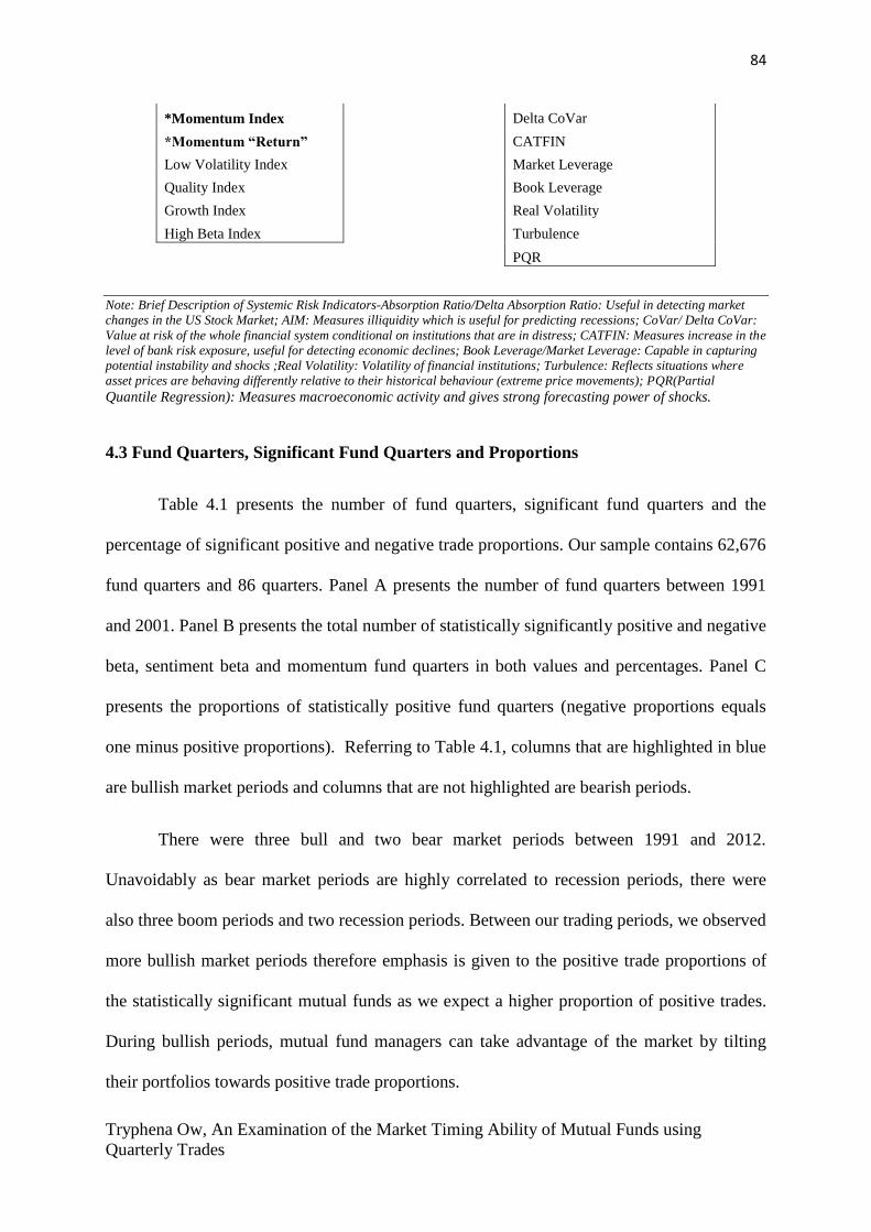
84
Tryphena Ow, An Examination of the Market Timing Ability of Mutual Funds using
Quarterly Trades
*Momentum Index Delta CoVar
*Momentum “Return”
CATFIN
Low Volatility Index
Market Leverage
Quality Index
Book Leverage
Growth Index
Real Volatility
High Beta Index
Turbulence
PQR
Note: Brief Description of Systemic Risk Indicators-Absorption Ratio/Delta Absorption Ratio: Useful in detecting market
changes in the US Stock Market; AIM: Measures illiquidity which is useful for predicting recessions; CoVar/ Delta CoVar:
Value at risk of the whole financial system conditional on institutions that are in distress; CATFIN: Measures increase in the
level of bank risk exposure, useful for detecting economic declines; Book Leverage/Market Leverage: Capable in capturing
potential instability and shocks ;Real Volatility: Volatility of financial institutions; Turbulence: Reflects situations where
asset prices are behaving differently relative to their historical behaviour (extreme price movements); PQR(Partial Quantile Regression): Measures macroeconomic activity and gives strong forecasting power of shocks.
4.3 Fund Quarters, Significant Fund Quarters and Proportions
Table 4.1 presents the number of fund quarters, significant fund quarters and the
percentage of significant positive and negative trade proportions. Our sample contains 62,676
fund quarters and 86 quarters. Panel A presents the number of fund quarters between 1991
and 2001. Panel B presents the total number of statistically significantly positive and negative
beta, sentiment beta and momentum fund quarters in both values and percentages. Panel C
presents the proportions of statistically positive fund quarters (negative proportions equals
one minus positive proportions). Referring to Table 4.1, columns that are highlighted in blue
are bullish market periods and columns that are not highlighted are bearish periods.
There were three bull and two bear market periods between 1991 and 2012.
Unavoidably as bear market periods are highly correlated to recession periods, there were
also three boom periods and two recession periods. Between our trading periods, we observed
more bullish market periods therefore emphasis is given to the positive trade proportions of
the statistically significant mutual funds as we expect a higher proportion of positive trades.
During bullish periods, mutual fund managers can take advantage of the market by tilting
their portfolios towards positive trade proportions.

85
Tryphena Ow, An Examination of the Market Timing Ability of Mutual Funds using
Quarterly Trades
To assist with the examination of market timing abilities, correlation and regression
tests will be conducted using the trade proportions of the statistically significant trades. Trade
beta proportions provide some insights on the behaviour of the mutual fund managers.
Quarters with a higher proportions of positive trades suggest a bullish market. In contrast,
quarters with a higher proportions of negative trades suggest a bearish market. Trade
proportions are calculated by dividing the number of positive trades over the total number of
positive and negative trades per quarter.
We observe from Panel A of Table 4.1 that fund quarters have substantially increased
over the years. Consistent to our expectations, as presented in Panel B of Table 4.1, there
were a higher number of significant positive beta and sentiment beta fund quarters exhibited
in each period. In contrast, we observe a higher number of significant negative momentum
fund quarters in each period. Similar to Panel B, Panel C of Table 4.1 exhibited a higher
proportion of statistically significant positive beta and sentiment beta fund quarters.
However, we observe a higher proportion of statistically significant negative momentum fund
quarters. Based on these observations, it is plausible that the mutual fund managers may have
chosen to pursue a contrarian strategy. Although we presumed that during bearish market
periods, there would be a higher proportion of negative fund quarters, we observe no
significant changes in the proportions of fund quarters between bullish and bearish periods.

86
Tryphena Ow, An Examination of the Market Timing Ability of Mutual Funds using Quarterly Trades
Table 4.1. Trades- Number of Fund Quarters, Significant Fund Quarters and Proportions
The number of observations of significant, non-significant fund quarters and proportions are provided below. We obtained the trade betas of US equity mutual funds from the data provided by
Cullen et al. (2015) for the period between June 1991 and September 2012. These fund quarters encompass beta, sentiment beta and momentum strategies and they are based on quarterly
data observations. Panel A presents the total number of fund quarters, Panel B presents the number of statistically significant positive and negative fund quarters and Panel C presents the
proportions of statistically significant positive fund quarters (one minus positive proportions equals negative proportions). The total number of fund quarters equals 62,676. Highlighted in
blue: Bull Market periods. Not highlighted: Bear Market Periods. Bear market periods are highly associated to Recession Periods.
1991 1992 1993 1994 1995 1996 1997 1998 1999 2000 2001 2002 2003 2004 2005 2006 2007 2008 2009 2010 2011 2012 1991-
2012
Panel A. Fund quarters
Total Fund Quarts 803 1,134 1,178 920 844 857 1,111 1,584 1,858 2,755 2,410 2,732 2,731 2,636 4,880 5,864 5,271 3,903 4,920 3,480 5,990 4,815 62,676
Panel B. Significant Fund quarters
Beta 13,836
Positive (Value) 119 145 112 91 86 65 118 177 281 521 415 388 387 316 464 584 445 365 1073 498 649 598 7,895
(%) 14.8 12.8 9.5 9.9 10.2 7.6 10.6 11.2 15.1 18.9 17.2 14.2 14.2 12.0 9.5 10.0 8.4 9.4 21.8 14.3 10.8 12.4 12.6
Negative (Value) 61 128 93 73 75 54 100 174 128 348 289 341 273 245 357 440 378 404 515 308 686 471 5,941
(%) 7.6 11.3 7.9 7.9 8.9 6.3 9.0 11.0 6.9 12.6 12.0 12.5 10.0 9.3 7.3 7.5 7.2 10.4 10.5 8.9 11.5 9.8 9.5
Sentiment Beta 10,810
Positive (Value) 117 158 146 98 64 94 171 202 259 529 440 395 364 316 515 599 429 335 679 237 159 6,306
(%) 14.6 13.9 12.4 10.7 7.6 11.0 15.4 12.8 13.9 19.2 18.3 14.5 13.3 12.0 10.6 10.2 8.1 8.6 13.8 6.8 2.7 10.1
Negative (Value) 55 123 103 70 104 84 97 125 171 403 274 356 258 241 328 417 376 341 324 183 71 4,504
(%) 6.8 10.8 8.7 7.6 12.3 9.8 8.7 7.9 9.2 14.6 11.4 13.0 9.4 9.1 6.7 7.1 7.1 8.7 6.6 5.3 1.2 7.2
Momentum 19,438
Positive (Value) 180 190 237 138 106 128 130 281 226 379 367 514 435 357 578 905 733 779 926 504 810 522 9,425
(%) 22.4 16.8 20.1 15.0 12.6 14.9 11.7 17.7 12.2 13.8 15.2 18.8 15.9 13.5 11.8 15.4 13.9 20.0 18.8 14.5 13.5 10.8 15.0
Negative (Value) 99 177 160 131 160 134 166 246 320 524 374 373 388 405 806 965 990 616 599 518 1040 822 10,013
(%) 12.3 15.6 13.6 14.2 19.0 15.6 14.9 15.5 17.2 19.0 15.5 13.7 14.2 15.4 16.5 16.5 18.8 15.8 12.2 14.9 17.4 17.1 16.0
Panel C. Statistically Significant Fund Quarters ( Proportions )
1991 1992 1993 1994 1995 1996 1997 1998 1999 2000 2001 2002 2003 2004 2005 2006 2007 2008 2009 2010 2011 2012
1991-
2012
Beta
Positive (%) 66.1 53.1 54.6 55.5 53.4 54.6 54.1 50.4 68.7 60.0 58.9 53.2 58.6 56.3 56.5 57.0 54.1 47.5 67.6 61.8 48.6 55.9 57.1
Sentiment
Positive (%) 68.0 56.2 58.6 58.3 38.1 52.8 63.8 61.8 60.2 56.8 61.6 52.6 58.5 56.7 61.1 59.0 53.3 49.6 67.7 56.4 69.1 58.3
Momentum
Positive (%) 64.5 51.8 59.7 51.3 39.8 48.9 43.9 53.3 41.4 42.0 49.5 57.9 52.9 46.9 41.8 48.4 42.5 55.8 60.7 49.3 43.8 38.8 48.4
Number of Fund Quarters, Significant Fund Quarters and Fund Quarters Proportions

87
Tryphena Ow, An Examination of the Market Timing Ability of Mutual Funds using
Quarterly Trades
4.3.1 Descriptive Statistics of Significant Fund Quarters and Proportions
Table 4.2 presents the descriptive statistics of the statistically significant fund quarters
and proportions. Panel A presents the descriptive statistics of positive and negative
statistically significant fund quarters. Panel B presents the descriptive statistics of positive
and negative fund quarter proportions. The mean and median values helps to determine if the
data are normally distributed or skewed. Skewed data occurs when the median and mean
values are significantly different.
We observe from Panel A of Table 4.2 that the mean and median values of the
statistically significant beta, sentiment beta and momentum fund quarters are not significantly
different. These implies that the fund quarters are normally distributed. Similarly, we observe
from Panel B that the proportions of fund quarters are normally distributed.
Table 4.2. Descriptive Statistics of Statistically Significant Fund Quarters and
Proportions
The descriptive statistics of statistically significant fund quarters and proportions are provided below. We
obtained the trade betas of US equity mutual funds from the data provided by Cullen et al. (2015) for the
period between June 1991 and September 2012. These fund quarters are based on quarterly data
observations. Panel A describes the statistically significant fund quarters of beta, sentiment beta and
momentum tilting. Panel B presents the proportions of beta, sentiment beta and momentum tilting fund
quarters. The total number of funds quarters equals 62,676.
Panel A: Significant Fund Quarters
Start Period End Period No. of Fund Quarters Mean Median
Beta Jun-91 Sep-12 13,836
Positive
7,895 359.0 376.0
Negative
5,941 270.0 281.0
Sentiment Beta Jun-91 Mar-11 10,810
Positive
6,306 300.3 259.0
Negative
4,504 214.5 183.0
Momentum Tilting Jun-91 Sep-12 19,438
Positive
9,425 428.4 373.0
Negative
10,013 455.1 381.0
(Panel B continues on next page)

88
Tryphena Ow, An Examination of the Market Timing Ability of Mutual Funds using
Quarterly Trades
Panel B. Proportion of Significant Fund quarters
Start Period End Period No. of Fund Quarters Mean Median
Beta Jun-91 Sep-12
Positive (%)
7,895 56.7 55.7
Negative (%)
5,941 43.3 44.3
Sentiment Jun-91 Mar-11
Positive (%) 6,306 58.1 58.5
Negative (%)
4,504 41.9 41.5
Momentum Jun-91 Sep-12
Positive (%)
9,425 49.3 49.1
Negative (%) 10,013 50.7 50.9
4.4 Descriptive Statistics of Market and Systemic Risk Indicators
4.4.1 Descriptive Statistics (In Months)
Table 4.3 and Table 4.4 presents the descriptive statistics of market and systemic risk
indicators we have considered for our analysis. We have considered 10 market indicators and
11 systemic risk indicators as they represent different components of the overall market and
the economy. Although the statistically significant trade betas are in calendar quarters, we
have presented the values of market and systemic risk indicators in both months (Table 4.3)
and quarters (Table 4.4) in order to examine if there are any substantial differences in their
mean and median values. This is to ensure that despite having a limited number of fund
quarter observations, results will not be affected.
Panel A of Table 4.3 and Table 4.4 presents the descriptive statistics of market
indicators that are related to the statistically significant trade proportions that encompass beta,
sentiment beta and momentum. Hereby known as “Main Market Indicators”, they are the
Market Index, Sentiment Index and Momentum Index. We have also constructed the “return”
indicators to avoid spurious issues. Typically market indices have constant increases or
decreases in their index values. Creating the “return” indicators allows us to standardise and

89
Tryphena Ow, An Examination of the Market Timing Ability of Mutual Funds using
Quarterly Trades
compare changes against the base values. “Returns” are calculated based on their respective
indices values in quarters, Eq. (1):
"Returns" = (𝐼𝑛𝑑𝑒𝑥 𝑉𝑎𝑙𝑢𝑒
𝑡1
𝐼𝑛𝑑𝑒𝑥 𝑉𝑎𝑙𝑢𝑒𝑡0− 1) ∗
360
4∗ 100 (1)
These indicators are the Market “Return”, Sentiment “Return” and Momentum “Return”
indicators. We expect “return” indicators to detect more changes in the index values.
Panel B of Table 4.3 and Table 4.4 presents the descriptive statistics of indicators that
are not directly related to the statistically significant trade proportions. However they provide
insights on the performance of other components of the market. Hereby known as “Sub-
Market Indicators”, they are the S&P Quality Index, S&P Growth Index, the S&P Low
Volatility Index and the S&P High Beta Index.
Panel C of Table 4.3 and Table 4.4 presents the descriptive statistics of systemic risk
indicators. These indicators help to predict macroeconomic outcomes. Recession indicators
are the Absorption ratio, Delta Absorption ratio, AIM and CATFIN. Indicators that signal
distress in financial institutions are CoVar, Delta CoVar and Real Volatility. Economic
instability or shocks indicators are the Book Leverage, Market Leverage and Real Volatility
and Partial Quantile Regression (PQR). Turbulence is an indicator that reflects shifts in asset
prices relative to their historical prices.
We observe from Panel A, Panel B and Panel C of Table 4.3, the momentum index,
the momentum “return” and the sub-market indicators have significantly lesser quarter
observations (over 70 quarters) compared to main market and systemic risk indicators (over
200 quarters). This was due to limited data availability as these indicators were recently
created in 2006.

90
Tryphena Ow, An Examination of the Market Timing Ability of Mutual Funds using
Quarterly Trades
Focusing on the mean and median values, we observe from Panel A of Table 4.3 that
all but the market “return”, sentiment “return” and momentum “return” indicators had similar
values. This suggests that the index values are normally distributed. As “return” indicators
measure changes in the index, skewed data is expected. Market “return”, sentiment “return”
and momentum “return” indicators have mean values that are lesser than the median, this
implies that “return” values are negatively skewed to the left. As these indicators measure
changes, it is reasonable to have skewed data as changes in the index values can range from
small to large values.
We observe from Panel B of Table 4.3 that all sub-market indicators have normally
distributed index values. We also observe from Panel C of Table 4.3 that all of the systemic
risk indicators have normally distributed values except for the Turbulence indicator with a
mean value significantly larger than the median. This suggest that the values of the
turbulence indicator is positively skewed to the right. As the turbulence indicator reflects
shifts in asset prices relative to their historical prices. It is likely to have skewed data as
changes could range from very small to very large changes.
Table 4.3. Descriptive Statistics of Market and Systemic Risk Indicators (Presented in
Months)
The descriptive statistics of the market and systemic risk indicators are provided below. For market
indicators, information is downloaded from Yahoo Finance, S&P website and Baker and Wurgler
website. For systemic risk indicators, information is downloaded from the Sethpruit website.
Quarterly data are presented in months. Panel A presents the descriptive statistics of the indices that
are directly related to the statistically significant trades also known as “Main Market Indicators”.
Panel B presents the descriptive statistics of the indices that are not directly related to the statistically
significant trades also known as “Sub-Market Indicators”. Panel C presents the descriptive statistics of
Systemic Risk Indicators.
Panel A: Main Market Indicators No. of Quarts Mean Median
Market Index (Jun 1991 - Sep 2012) 256 998.27 1103.00
Market “Return” (Jul 1991- Sep 2012) (% p.q) 255 7.21 12.18
Sentiment Index (Jun 1991 - Sep 2012) 256 0.30 0.26
Sentiment “Return” (Jul 1991- Sep 2012) 255 0.15 -0.15
Momentum Index (Sep 2006- Sep 2012) 73 377.29 391.99
Momentum “Return” (Oct 2006- Sep 2012) (%p.q) 72 1.48 6.44
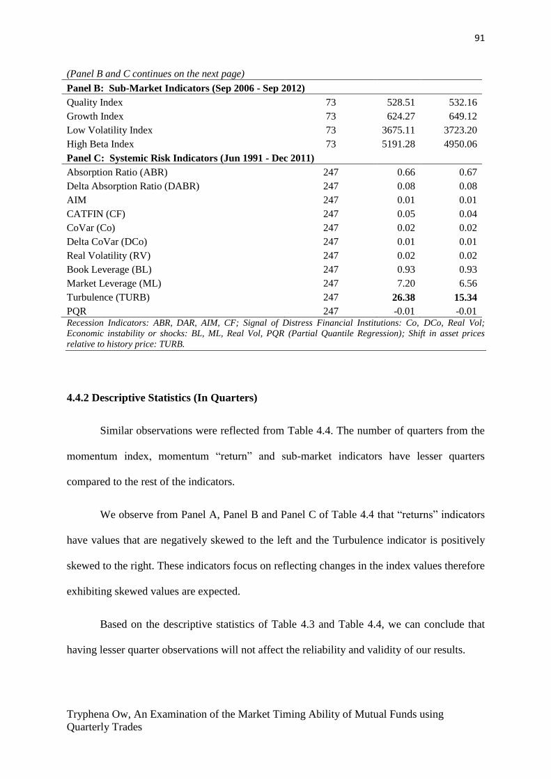
91
Tryphena Ow, An Examination of the Market Timing Ability of Mutual Funds using
Quarterly Trades
(Panel B and C continues on the next page)
Panel B: Sub-Market Indicators (Sep 2006 - Sep 2012)
Quality Index 73 528.51 532.16
Growth Index 73 624.27 649.12
Low Volatility Index 73 3675.11 3723.20
High Beta Index 73 5191.28 4950.06
Panel C: Systemic Risk Indicators (Jun 1991 - Dec 2011)
Absorption Ratio (ABR) 247 0.66 0.67
Delta Absorption Ratio (DABR) 247 0.08 0.08
AIM 247 0.01 0.01
CATFIN (CF) 247 0.05 0.04
CoVar (Co) 247 0.02 0.02
Delta CoVar (DCo) 247 0.01 0.01
Real Volatility (RV) 247 0.02 0.02
Book Leverage (BL) 247 0.93 0.93
Market Leverage (ML) 247 7.20 6.56
Turbulence (TURB) 247 26.38 15.34
PQR 247 -0.01 -0.01 Recession Indicators: ABR, DAR, AIM, CF; Signal of Distress Financial Institutions: Co, DCo, Real Vol;
Economic instability or shocks: BL, ML, Real Vol, PQR (Partial Quantile Regression); Shift in asset prices
relative to history price: TURB.
4.4.2 Descriptive Statistics (In Quarters)
Similar observations were reflected from Table 4.4. The number of quarters from the
momentum index, momentum “return” and sub-market indicators have lesser quarters
compared to the rest of the indicators.
We observe from Panel A, Panel B and Panel C of Table 4.4 that “returns” indicators
have values that are negatively skewed to the left and the Turbulence indicator is positively
skewed to the right. These indicators focus on reflecting changes in the index values therefore
exhibiting skewed values are expected.
Based on the descriptive statistics of Table 4.3 and Table 4.4, we can conclude that
having lesser quarter observations will not affect the reliability and validity of our results.

92
Tryphena Ow, An Examination of the Market Timing Ability of Mutual Funds using
Quarterly Trades
Table 4.4. Descriptive Statistics of Market and Systemic Risk Indicators (Presented in
Quarters)
The descriptive statistics of the market and systemic risk indicators are provided below. For market
indicators, information is downloaded from Yahoo Finance, S&P website and Baker and Wurgler
website. For systemic risk indicators, information is downloaded from the Sethpruit website.
Quarterly data are presented in quarters. Panel A presents the descriptive statistics of the indices that
are directly related to the statistically significant trades also known as “Main Market Indicators”.
Panel B presents the descriptive statistics of the indices that are not directly related to the statistically
significant trades also known as “Sub-Market Indicators”. Panel C presents the descriptive statistics of
Systemic Risk Indicators.
Panel A: Main Market Indicators No. of Quarts Mean Median
Market Index (Jun 1991 - Sep 2012) 86 995.19 1094.86
Market “Return” (Jul 1991- Sep 2012) (% p.q) 85 7.45 9.68
Sentiment Index (Jun 1991 - Sep 2012) 86 0.32 0.30
Sentiment “Return” (Jul 1991-Sep 2012) 85 0.65 -0.08
Momentum Index (Sep 2006 - Sep 2012) 25 374.98 391.14
Momentum “Return” (Oct 2006-Sep 2012) (%p.q) 24 4.85 9.73
Panel B: S&P Sub-Market Indicators (Period: Sep 2006 - Sep 2012)
Quality Index 25 524.97 537.90
Growth Index 25 620.65 642.17
Low Volatility Index 25 3662.86 3704.60
High Beta Index 25 5156.52 4850.51
Panel C: Systemic Risk Indicators (Jun 1991 - Dec 2011)
Absorption Ratio (ABR) 83 0.66 0.67
Delta Absorption Ratio (DABR) 83 0.08 0.09
AIM 83 0.01 0.01
CATFIN (CF) 83 0.05 0.04
CoVar (Co) 83 0.02 0.02
Delta CoVar (DCo) 83 0.01 0.01
Book Leverage (BL) 83 0.93 0.93
Market Leverage (ML) 83 7.20 6.46
Real Volatility (RV) 83 0.02 0.02
Turbulence (TURB) 83 28.73 14.54
PQR 83 -0.01 -0.01 Recession Indicators: ABR, DAR, AIM, CF; Signal of Distress Financial Institutions: Co, DCo, Real Vol;
Economic instability or shocks: BL, ML, Real Vol, PQR (Partial Quantile Regression); Shift in asset prices
relative to history price: TURB.

93
Tryphena Ow, An Examination of the Market Timing Ability of Mutual Funds using
Quarterly Trades
4.5 Performance of Market Indicators
Studying the performance of market indicators allows us to understand how the
market behaves during bullish and bearish markets. Between June 1991 and September 2012,
there were three bull and two bull market periods.
The three periods of bull markets are as follows, July 1991 to January 2000, October
2002 to October 2007 and March 2009 to October 2012. The two periods of bear markets are
as follows, January 2000 to October 2002 and October 2007 to March 2009.
Amadeo (2016) reported that bear periods are highly correlated to recession periods as
an economic decline usually leads to a widespread of falling securities prices. During bear
and recession periods, we expect to see plunges in the values of the main market indicators.
In contrast, during bull and boom periods, we expect to see increasing index values of the
main market indicators. Graph 4.1 to 4.6 reflects changes in index values during bull and bear
market periods.
Graph 4.1: Price fluctuations of the Market Index, June 1991 to September 2012
The graph below presents the values of the market index based on quarterly opening prices. The
market index is a reflector of 500 stocks in the US equity market. Index values are presented in
quarters.
0.00
200.00
400.00
600.00
800.00
1000.00
1200.00
1400.00
1600.00
1800.00
1/6
/19
91
1/1
2/1
99
11
/6/1
992
1/1
2/1
99
21
/6/1
993
1/1
2/1
99
31
/6/1
994
1/1
2/1
99
41
/6/1
995
1/1
2/1
99
51
/6/1
996
1/1
2/1
99
61
/6/1
997
1/1
2/1
99
71
/6/1
998
1/1
2/1
99
81
/6/1
999
1/1
2/1
99
91
/6/2
000
1/1
2/2
00
01
/6/2
001
1/1
2/2
00
11
/6/2
002
1/1
2/2
00
21
/6/2
003
1/1
2/2
00
31
/6/2
004
1/1
2/2
00
41
/6/2
005
1/1
2/2
00
51
/6/2
006
1/1
2/2
00
61
/6/2
007
1/1
2/2
00
71
/6/2
008
1/1
2/2
00
81
/6/2
009
1/1
2/2
00
91
/6/2
010
1/1
2/2
01
01
/6/2
011
1/1
2/2
01
11
/6/2
012
Market Index (Quarterly Observations)
Jun 1991- Sep 2012
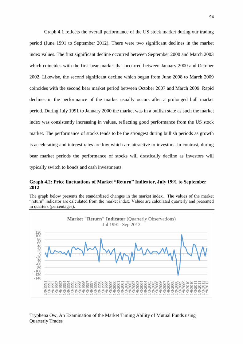
94
Tryphena Ow, An Examination of the Market Timing Ability of Mutual Funds using
Quarterly Trades
Graph 4.1 reflects the overall performance of the US stock market during our trading
period (June 1991 to September 2012). There were two significant declines in the market
index values. The first significant decline occurred between September 2000 and March 2003
which coincides with the first bear market that occurred between January 2000 and October
2002. Likewise, the second significant decline which began from June 2008 to March 2009
coincides with the second bear market period between October 2007 and March 2009. Rapid
declines in the performance of the market usually occurs after a prolonged bull market
period. During July 1991 to January 2000 the market was in a bullish state as such the market
index was consistently increasing in values, reflecting good performance from the US stock
market. The performance of stocks tends to be the strongest during bullish periods as growth
is accelerating and interest rates are low which are attractive to investors. In contrast, during
bear market periods the performance of stocks will drastically decline as investors will
typically switch to bonds and cash investments.
Graph 4.2: Price fluctuations of Market “Return” Indicator, July 1991 to September
2012
The graph below presents the standardized changes in the market index. The values of the market
“return” indicator are calculated from the market index. Values are calculated quarterly and presented
in quarters (percentages).
-140-120-100
-80-60-40-20
020406080
100120
1/9
/19
91
1/3
/19
92
1/9
/19
92
1/3
/19
93
1/9
/19
93
1/3
/19
94
1/9
/19
94
1/3
/19
95
1/9
/19
95
1/3
/19
96
1/9
/19
96
1/3
/19
97
1/9
/19
97
1/3
/19
98
1/9
/19
98
1/3
/19
99
1/9
/19
99
1/3
/20
00
1/9
/20
00
1/3
/20
01
1/9
/20
01
1/3
/20
02
1/9
/20
02
1/3
/20
03
1/9
/20
03
1/3
/20
04
1/9
/20
04
1/3
/20
05
1/9
/20
05
1/3
/20
06
1/9
/20
06
1/3
/20
07
1/9
/20
07
1/3
/20
08
1/9
/20
08
1/3
/20
09
1/9
/20
09
1/3
/20
10
1/9
/20
10
1/3
/20
11
1/9
/20
11
1/3
/20
12
1/9
/20
12
Market "Return" Indicator (Quarterly Observations)
Jul 1991- Sep 2012

95
Tryphena Ow, An Examination of the Market Timing Ability of Mutual Funds using
Quarterly Trades
Based on Graph 4.2, the market “return” indicator has fluctuated drastically during the
trading period. As the market index only reflects “surface” changes which has consecutive
positive values, the market “return” indicator is a better standard for reflecting specifically
how much changes there were in each quarter or how much has the index increased or
decreased in values. There was a significant decline in market returns between December
1997 and September 1998 followed by a significant increase in market returns between
September 1998 and December 1999. This could be a warning signal for an upcoming
bearish market. The first bear period occurred between January 2000 and October 2002.
When the market is bullish, it usually goes through a peak period and the economy is running
at full steam. Employment levels are at peak level with high GDP output and high inflation
levels. However, such economy progress will be stalled and contracted as wages and prices of
goods are inflexible to change. This will result in a market crash and involuntarily leads to a
bear market period.
The recovery of a bear period usually results in a sharp rise in market prices with an
accelerating growth rate. This is because the base values of opening prices usually drops to a
new low. Also to help with economy recovery, credit conditions are usually less strict to ease
monetary policies in order to create a healthy environment for rapid margin expansion and
profit growth.
Similarly, we observe a significant decline in market returns between March 2008 and
December 2008, followed by a drastic increase in market returns between December 2008
and December 2009 and another decline between December 2009 and September 2010. This
changes could be associated to the occurrence of the second bear market period that happened
between October 2007 and March 2009.
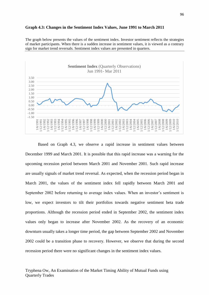
96
Tryphena Ow, An Examination of the Market Timing Ability of Mutual Funds using
Quarterly Trades
Graph 4.3: Changes in the Sentiment Index Values, June 1991 to March 2011
The graph below presents the values of the sentiment index. Investor sentiment reflects the strategies
of market participants. When there is a sudden increase in sentiment values, it is viewed as a contrary
sign for market trend reversals. Sentiment index values are presented in quarters.
Based on Graph 4.3, we observe a rapid increase in sentiment values between
December 1999 and March 2001. It is possible that this rapid increase was a warning for the
upcoming recession period between March 2001 and November 2001. Such rapid increase
are usually signals of market trend reversal. As expected, when the recession period began in
March 2001, the values of the sentiment index fell rapidly between March 2001 and
September 2002 before returning to average index values. When an investor’s sentiment is
low, we expect investors to tilt their portfolios towards negative sentiment beta trade
proportions. Although the recession period ended in September 2002, the sentiment index
values only began to increase after November 2002. As the recovery of an economic
downturn usually takes a longer time period, the gap between September 2002 and November
2002 could be a transition phase to recovery. However, we observe that during the second
recession period there were no significant changes in the sentiment index values.
-1.50
-1.00
-0.50
0.00
0.50
1.00
1.50
2.00
2.50
3.00
3.50
1/6
/19
91
1/1
2/1
99
1
1/6
/19
92
1/1
2/1
99
21
/6/1
993
1/1
2/1
99
31
/6/1
994
1/1
2/1
99
41
/6/1
995
1/1
2/1
99
5
1/6
/19
96
1/1
2/1
99
61
/6/1
997
1/1
2/1
99
7
1/6
/19
98
1/1
2/1
99
8
1/6
/19
99
1/1
2/1
99
9
1/6
/20
00
1/1
2/2
00
0
1/6
/20
01
1/1
2/2
00
11
/6/2
002
1/1
2/2
00
21
/6/2
003
1/1
2/2
00
31
/6/2
004
1/1
2/2
00
4
1/6
/20
05
1/1
2/2
00
51
/6/2
006
1/1
2/2
00
6
1/6
/20
07
1/1
2/2
00
7
1/6
/20
08
1/1
2/2
00
81
/6/2
009
1/1
2/2
00
9
1/6
/20
10
1/1
2/2
01
0
Sentiment Index (Quarterly Observations)
Jun 1991- Mar 2011

97
Tryphena Ow, An Examination of the Market Timing Ability of Mutual Funds using
Quarterly Trades
Graph 4.4: Changes in the values of the Sentiment “Return” Indicator, July 1991 to
March 2011
The graph below presents the standardized changes in the sentiment index. The values of the
sentiment “return” indicators are calculated from the sentiment index. Values are calculated quarterly
and presented in quarters.
Graph 4.4 presents the standardized changes of the sentiment index. Although the
sentiment index has frequent positive and negative index values, it is plausible that the
sentiment “return” would be a better reflector of sentiment changes. The sentiment index
specifically reflects the differences in the index values in each quarter.
Compared to the sentiment index (Graph 4.3), there were two distinct series of returns
fluctuations. We observe that between September 1998 and June 1999, the sentiment returns
had fallen drastically but increased significantly between June 1999 and December 1999.
Such changes could suggest an upcoming economy downturn. We observe that the sentiment
returns reverted to average values between December 1999 and June 2000. It is plausible that
this changes are related to the first recession period between March 2001 and November
2001.
We also observe that between September 1998 and June 1999, sentiment returns had
significantly increase before falling back to average return values between December 2008
and June 2009. This fluctuation of returns could also be associated with the second recession
-60.00
-40.00
-20.00
0.00
20.00
40.00
60.00
80.00
1/9
/19
91
1/3
/19
92
1/9
/1992
1/3
/19
93
1/9
/1993
1/3
/19
94
1/9
/19
94
1/3
/19
95
1/9
/19
95
1/3
/19
96
1/9
/19
96
1/3
/19
97
1/9
/19
97
1/3
/19
98
1/9
/19
98
1/3
/19
99
1/9
/19
99
1/3
/20
00
1/9
/20
00
1/3
/20
01
1/9
/20
01
1/3
/20
02
1/9
/20
02
1/3
/20
03
1/9
/20
03
1/3
/20
04
1/9
/20
04
1/3
/20
05
1/9
/20
05
1/3
/2006
1/9
/20
06
1/3
/2007
1/9
/20
07
1/3
/20
08
1/9
/20
08
1/3
/20
09
1/9
/20
09
1/3
/20
10
1/9
/20
10
1/3
/20
11
Sentiment "Return" Indicator (Quarterly Observations)
Jul 1991- Mar 2011
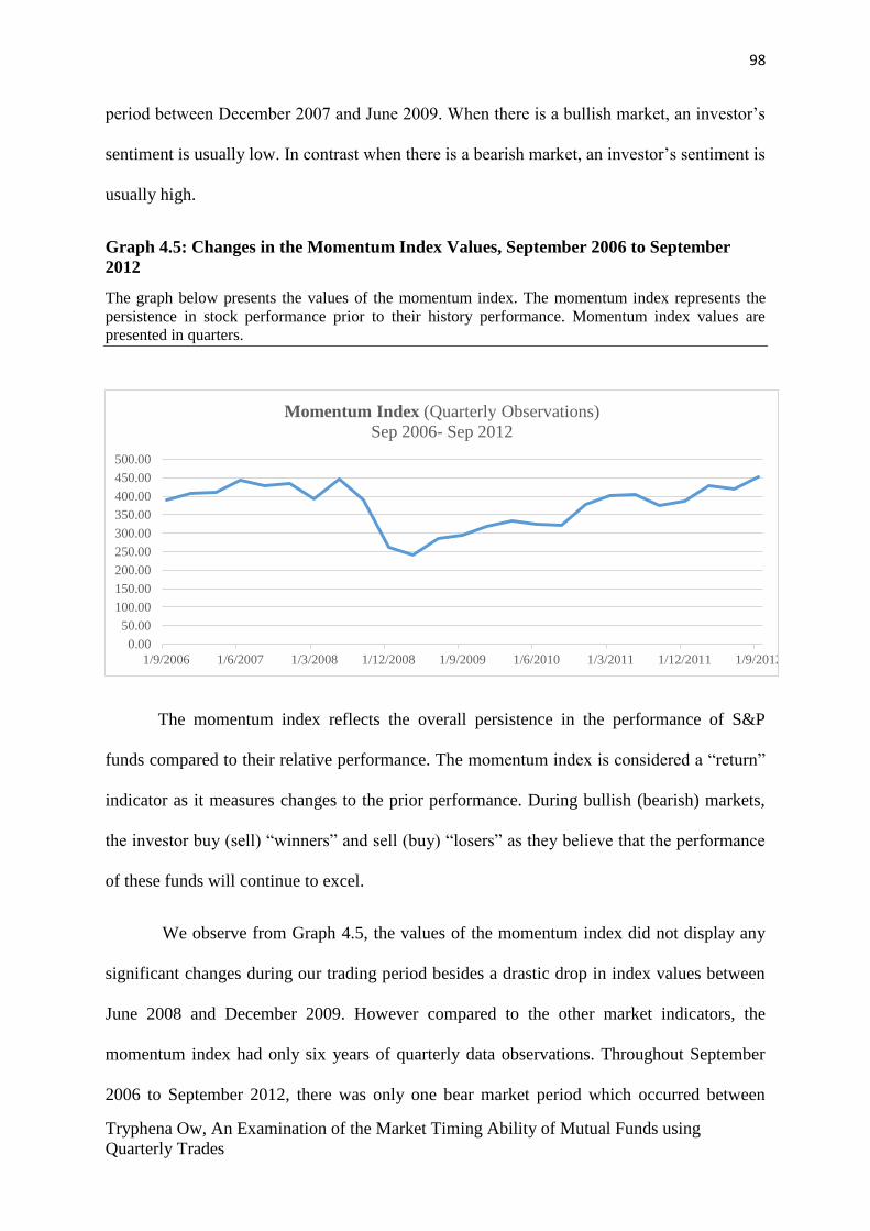
98
Tryphena Ow, An Examination of the Market Timing Ability of Mutual Funds using
Quarterly Trades
period between December 2007 and June 2009. When there is a bullish market, an investor’s
sentiment is usually low. In contrast when there is a bearish market, an investor’s sentiment is
usually high.
Graph 4.5: Changes in the Momentum Index Values, September 2006 to September
2012
The graph below presents the values of the momentum index. The momentum index represents the
persistence in stock performance prior to their history performance. Momentum index values are
presented in quarters.
The momentum index reflects the overall persistence in the performance of S&P
funds compared to their relative performance. The momentum index is considered a “return”
indicator as it measures changes to the prior performance. During bullish (bearish) markets,
the investor buy (sell) “winners” and sell (buy) “losers” as they believe that the performance
of these funds will continue to excel.
We observe from Graph 4.5, the values of the momentum index did not display any
significant changes during our trading period besides a drastic drop in index values between
June 2008 and December 2009. However compared to the other market indicators, the
momentum index had only six years of quarterly data observations. Throughout September
2006 to September 2012, there was only one bear market period which occurred between
0.00
50.00
100.00
150.00
200.00
250.00
300.00
350.00
400.00
450.00
500.00
1/9/2006 1/6/2007 1/3/2008 1/12/2008 1/9/2009 1/6/2010 1/3/2011 1/12/2011 1/9/2012
Momentum Index (Quarterly Observations)
Sep 2006- Sep 2012
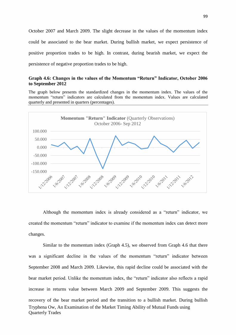
99
Tryphena Ow, An Examination of the Market Timing Ability of Mutual Funds using
Quarterly Trades
October 2007 and March 2009. The slight decrease in the values of the momentum index
could be associated to the bear market. During bullish market, we expect persistence of
positive proportion trades to be high. In contrast, during bearish market, we expect the
persistence of negative proportion trades to be high.
Graph 4.6: Changes in the values of the Momentum “Return” Indicator, October 2006
to September 2012
The graph below presents the standardized changes in the momentum index. The values of the
momentum “return” indicators are calculated from the momentum index. Values are calculated
quarterly and presented in quarters (percentages).
Although the momentum index is already considered as a “return” indicator, we
created the momentum “return” indicator to examine if the momentum index can detect more
changes.
Similar to the momentum index (Graph 4.5), we observed from Graph 4.6 that there
was a significant decline in the values of the momentum “return” indicator between
September 2008 and March 2009. Likewise, this rapid decline could be associated with the
bear market period. Unlike the momentum index, the “return” indicator also reflects a rapid
increase in returns value between March 2009 and September 2009. This suggests the
recovery of the bear market period and the transition to a bullish market. During bullish
-150.000
-100.000
-50.000
0.000
50.000
100.000
Momentum "Return" Indicator (Quarterly Observations)
October 2006- Sep 2012

100
Tryphena Ow, An Examination of the Market Timing Ability of Mutual Funds using
Quarterly Trades
market, we expect momentum “returns” to be high. In contrast, during bearish market, we
expect the “momentum” returns to be low.
4.6 Correlation Testing
Correlation testing is important for our study as it measures the degree to which two
variables move in relation to each other. The main variables in our study are the statistically
significant trade proportions (dependent variable) and the market and systemic risk indicators
(independent variables). There are three types of correlation analysis, Pearson Correlation,
Kendall Correlation and Spearman Correlation.
Based on Lee and Peters (2015), the Pearson correlation measures the degree of the
relationship between linear related variables and these variables are assumed to be normally
distributed. The Kendall correlation is a non-parametric test that measures the strength
between two variables and also test similarities in the ordering of data when it is ranked by
qualities. The Spearman correlation is also a non-parametric test that is used to measure the
degree of association between two variables. The difference between the Pearson correlation
and the Spearman correlation is that the Spearman Correlation measures non-linear
relationships and variables are measured on a scale that is at least ordinal. A high correlation
value ranges from ±0.5 to ±1.0, medium correlation ranges from ±0.3 to ±0.5 and a low
correlation ranges from ±0.1 to ±0.3. Having a positive (negative) high correlation value
implies that when one variable moves, the other variable moves in lockstep in the same
(opposite) direction. Also, the significant levels (p-values) of the correlation results are
important to determine if the correlation between the variables are not the results of chance or
random sampling error.
In this study, we will be using the Pearson correlation analysis as most of our data
observations are normally distributed.

101
Tryphena Ow, An Examination of the Market Timing Ability of Mutual Funds using
Quarterly Trades
4.6.1 Correlation Testing between Market Indicators (Main Market Indicators and
Sub-Market Indicators)
Considering a wide range of market indicators allow us to have a comprehensive
study of the market movements and they reflect bullish and bearish market trends. We study
the relationship between these indicators to determine if they are moving in the same
direction therefore reflecting similar market performances. If these market indicators are
highly correlated, we are able to conclude that they are moving in accordance during changes
in market trends. Emphasis is given to the main market indicators which are the Market
Index, Sentiment Index and Momentum Index as they are directly related to the statistically
significant trades that encompass beta, sentiment beta and momentum.
A correlation test would also be conducted between the main market indicators and
the sub-market indicators which are the Quality Index, Growth Index, Low Volatility Index,
and High Beta Index. This is to ensure that these indicators are all moving in accordance to
the market hence reflecting similar behaviour of market trends and performances.
Correlation analysis will not be conducted between the “return” indicators as they do
not reflect the overall performance of the market but reflect the quarterly period changes in
their respective indicators.
Table 4.5 presents the two correlation results, firstly between the main market
indicators and secondly between the main market indicators and sub-market indicators.
Results are presented in months and quarters to ensure that despite lesser number of fund
quarters, results will not be affected. Panel A presents the results of the correlation test
between the main market indicators in months. Panel B presents the results of the correlation
test between the main market and sub-market indicators in months. Panel C presents the
results of the correlation test between the main market indicators in quarters. Panel D
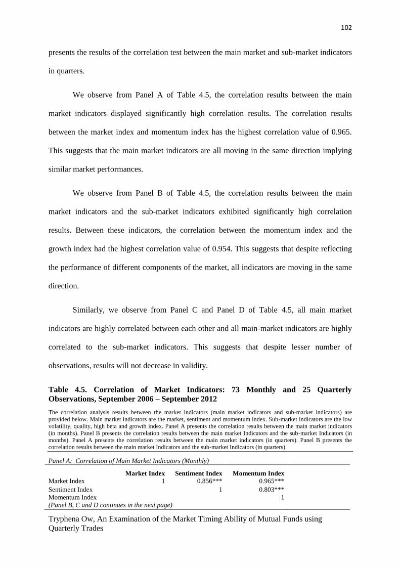
102
Tryphena Ow, An Examination of the Market Timing Ability of Mutual Funds using
Quarterly Trades
presents the results of the correlation test between the main market and sub-market indicators
in quarters.
We observe from Panel A of Table 4.5, the correlation results between the main
market indicators displayed significantly high correlation results. The correlation results
between the market index and momentum index has the highest correlation value of 0.965.
This suggests that the main market indicators are all moving in the same direction implying
similar market performances.
We observe from Panel B of Table 4.5, the correlation results between the main
market indicators and the sub-market indicators exhibited significantly high correlation
results. Between these indicators, the correlation between the momentum index and the
growth index had the highest correlation value of 0.954. This suggests that despite reflecting
the performance of different components of the market, all indicators are moving in the same
direction.
Similarly, we observe from Panel C and Panel D of Table 4.5, all main market
indicators are highly correlated between each other and all main-market indicators are highly
correlated to the sub-market indicators. This suggests that despite lesser number of
observations, results will not decrease in validity.
Table 4.5. Correlation of Market Indicators: 73 Monthly and 25 Quarterly
Observations, September 2006 – September 2012
The correlation analysis results between the market indicators (main market indicators and sub-market indicators) are
provided below. Main market indicators are the market, sentiment and momentum index. Sub-market indicators are the low
volatility, quality, high beta and growth index. Panel A presents the correlation results between the main market indicators
(in months). Panel B presents the correlation results between the main market Indicators and the sub-market Indicators (in
months). Panel A presents the correlation results between the main market indicators (in quarters). Panel B presents the
correlation results between the main market Indicators and the sub-market Indicators (in quarters).
Panel A: Correlation of Main Market Indicators (Monthly)
Market Index Sentiment Index Momentum Index
Market Index 1 0.856*** 0.965***
Sentiment Index
1 0.803***
Momentum Index
1
(Panel B, C and D continues in the next page)

103
Tryphena Ow, An Examination of the Market Timing Ability of Mutual Funds using
Quarterly Trades
Panel B: Correlation of Main Market Indices and Sub-Market Indicators (Monthly)
Low volatility Index Quality Index High Beta Index Growth Index
Market Index 0.883*** 0.848*** 0.894*** 0.917***
Sentiment Index 0.738*** 0.614*** 0.833*** 0.710***
Momentum Index 0.911*** 0.901*** 0.785*** 0.954***
Panel C: Correlation of Main Indicators (Quarterly)
Market Index Sentiment Index Momentum Index
Market Index 1 0.853*** 0.972***
Sentiment Index
1 0.799***
Momentum Index
1
Panel D: Correlation of Main Market Indicators and Sub-Market Indicators (Quarterly)
Low volatility Index Quality Index High Beta Index Growth Index
Market Index 0.893*** 0.858*** 0.883*** 0.92***
Sentiment Index 0.744*** 0.618*** 0.843*** 0.703***
Momentum Index 0.927*** 0.910*** 0.782*** 0.956***
*** Significant at the 0.01 level
** Significant at the 0.05 level
* Significant at the 0.10 level
4.6.2 Correlation Testing between Systemic Risk Indicators
We have considered all 19 systemic risk indicators and selected 11 indicators that are
most insightful in measuring risk in the real economy. Fluctuations in systemic risk signals
changes in the economy and impacts the probability of an economic downturn. Systemic risk
indicators are useful in reflecting recession market trends. When there are changes in the
values of these systemic risk indicators, it serves as a warning for upcoming economic
changes.
4.6.2.1 Brief Description of the Selected Systemic Risk Indicators
We have selected the Absorption ratio, Delta Absorption ratio, AIM, CoVar, Delta
CoVar, Book Leverage, Market Leverage, Real Volatility, CATFIN, Turbulence and the PQR
indicators.

104
Tryphena Ow, An Examination of the Market Timing Ability of Mutual Funds using
Quarterly Trades
Primary recession indicators are the Absorption ratio, Delta Absorption ratio, AIM
and the CATFIN. The Absorption ratio is useful in detecting US market changes. When there
is a high absorption ratio, it implies that the market is vulnerable. The Delta Absorption ratio
measures “changes”, it captures shifts in short term absorption ratio relative to the long term
absorption ratio. AIM reflects the illiquidity in an economy. It has been successful in
predicting recession as liquidity tends to fall before a recession. CATFIN reflects the level of
risk a bank is expose to, this ratio is very useful in detecting economic declines.
Indicators that monitor the performance of financial institutions are the CoVar, Delta
CoVar and Real Volatility indicators. CoVar is the value at risk of a distress financial
institution. Delta CoVar captures how much a particular institution has contributed to the
overall systemic risk. Real Volatility measures the volatility of financial institutions.
Primary economic instability indicators are the Book Leverage, Market Leverage and
the PQR indicators. Book and Market Leverage are useful in capturing instability and shocks.
The PQR indicator gives strong forecasting power of macroeconomic shocks in the economy.
Lastly, Turbulence ratio captures the shift in asset prices relative to their historical price.
When asset prices display extreme changes, this signals an economic downturn.
A correlation test was conducted between these 11 systemic risk indicators to identify
which indicators are highly and lowly correlated, in both positive and negative values.
Selecting these indicators gives us a broader understanding of how highly correlated or
negatively correlated trades can affect the trading movements of the statistically significant
trades.
Table 4.6 presents the results of the correlations analysis between 11 of the systemic
risk indicators in months and quarters. Panel A presents the results of the correlation analysis
in months. Panel B presents the results of the correlation analysis in quarters. Similar to the

105
Tryphena Ow, An Examination of the Market Timing Ability of Mutual Funds using
Quarterly Trades
correlation test between the market indicators, conducting the correlation test using monthly
and quarterly data observations ensures the validity of our results.
We observe from Panel A and Panel B of Table 4.6 that most of the systemic risk
indicators displayed high correlations values that are significant at the 0.01 level. Comparing
the results of Panel A and Panel B, we did not observe any significant differences in the
values of the correlation analysis. Therefore, having a lesser number of data observations will
not affect the reliability of our results.
Table 4.6. Correlation between Systemic Risk Indicators: 247 Monthly Observations
and 83 Quarterly Observations, June 1991 to December 2011 The results of the correlation analysis between the 11 of the systemic risk indicators are provided below. Panel A presents
the results of the correlation analysis between the 11 of the systemic risk Indicators (in months). Panel B presents the results
of the correlation analysis between the 11 of the systemic risk indicators (in quarters). Primary Recession Indicators: ABR,
DABR, AIM, CF; Signal of Distress Financial Institutions: Co, DCo, Real Vol; Economic instability or shocks: BL, ML,
PQR; Shift in asset prices relative to history price: TURB. The data covers the period between 1991 and 2011.
Panel A: Monthly Observations
ABR DABR AIM Co DCo BL ML RV TURB CF PQR
ABR 1 -0.40*** -0.20*** 0.78*** 0.81*** 0.30*** 0.45*** 0.46*** 0.29*** 0.44*** -0.32***
DABR
1 0.21*** -0.33*** -0.33*** -0.06 -0.08 0.06 -0.03 0.06 0.00
AIM
1 -0.10 -0.13** 0.00 -0.16** 0.03 -0.03 0.01 -0.02
Co
1 0.96*** 0.20*** 0.56*** 0.65*** 0.33*** 0.62*** -0.47***
DCo
1 0.12 0.66*** 0.57*** 0.29*** 0.55*** -0.37***
BL
1 0.06 0.16** 0.20*** 0.15** -0.21***
ML
1 0.42*** 0.31*** 0.48*** -0.30***
RV
1 0.72*** 0.31*** -0.71***
TURB
1 0.76*** -0.71***
CF
1 -0.64***
PQR
1
Panel B: Quarterly Observations
ABR DABR AIM Co DCo BL ML RV TURB CF PQR
ABR 1 -0.34*** -0.25*** 0.77*** 0.80*** 0.32*** 0.53*** 0.47*** 0.30*** 0.45*** -0.34***
DABR
1 0.26** -0.31*** -0.31*** -0.01 -0.08 0.09 0.00 0.07 -0.07
AIM
1 -0.15 -0.17 -0.01 -0.14 -0.03 -0.04 -0.03 0.03
Co
1 0.96*** 0.22** 0.57*** 0.60*** 0.26** 0.56*** -0.45***
DCo
1 0.15 0.67*** 0.52*** 0.21 0.56*** -0.37***
BL
1 0.06 0.19 0.20 0.21 -0.14
ML
1 0.39*** 0.23*** 0.46*** -0.28***
RV
1 0.79*** 0.84*** -0.62***
TURB
1 0.84*** -0.37***
CF
1 -0.52***
PQR 1

106
Tryphena Ow, An Examination of the Market Timing Ability of Mutual Funds using
Quarterly Trades
ABR: Absorption Ratio, DABR: Delta Absorption Ratio, Co: CoVar; Dco: Delta CoVar, BL: Book Leverage,
ML: Market Leverage, CF: CATFIN, TURB: Turbulence PQR: Partial Quantile Regression
*** Significant at the 0.01 level
** Significant at the 0.05 level
* Significant at the 0.10 level
In order to have an optimal analysis process, we are interested in correlation values of
indicators that that are significant at the 0.01 level and they being replaced by correlation
symbols and presented in Table 4.7, Panel A.
Panel A presents the level of correlation between the systemic risk indicators that
have exhibited correlation results that are significant at the 0.01 level and they are presented
in these symbols: 𝐶𝐻±, 𝐶𝑀± and 𝐶𝐿±. High correlation value is denoted by 𝐶𝐻±, Medium
correlation value is denoted by 𝐶𝑀±and Low correlation value is denoted by 𝐶𝐿±. A high
correlation value ranges from ±0.6-1.0, a medium correlation value ranges from ±0.3-0.6 and
a low correlation value ranges from ±0.1-0.3. Panel B presents the highest positive and
negative correlated values and the lowest positive and negative correlated values of the
systemic risk indicators (in bold).
We observe from Panel B of Table 4.7, the lowest negative correlation was between
the Absorption Ratio and AIM indicators with a correlation value of -0.25. The highest
negative correlation was between Real Volatility and PQR indicators with a correlation value
of -0.62. The lowest positive correlation was between Market Leverage and Turbulence
indicators with a correlation value of 0.23. The highest positive correlation was between
CoVar and Delta CoVar indicators with a correlation value of 0.96.
Between these indicators, the Absorption ratio and AIM are both recession indicators.
As the Absorption ratio and Delta Absorption ratio are similar measures of upcoming
recession periods, we have decided to select the Delta Absorption ratio for the final analysis

107
Tryphena Ow, An Examination of the Market Timing Ability of Mutual Funds using
Quarterly Trades
as the Delta Absorption ratio captures the changes between the short term and long term
absorption ratios therefore avoids spurious issues. Similarly as CoVar, Delta CoVar and Real
Volatility indicators tracks the performance of financial institutions, we have selected the
Delta CoVar indicator to avoid spurious issues as we expect Delta CoVar indicator reflects
the differences in CoVar conditional on a distress institution and a normal state of the
institution. The Market Leverage and PQR indicators are measures of economic instability.
We have selected the PQR indicator as it is the accumulated information of the systemic risk
measures. It is a better indicator as it gives a stronger forecasting power of macroeconomic
shocks.
Therefore, the final selection of systemic risk indicators are the Delta Absorption
Ratio, Delta CoVar, PQR and Turbulence indicators.
Table 4.7. Significant (at 0.01 Level) results of Positive and Negative Correlations
between the Selected Systemic Risk Indicators: 83 Quarterly Observations, June 1991 to
December 2011
The results of the correlation analysis between 11 of the systemic risk indicators that are significant at
the 0.01 level are provided below. Panel A presents the symbols of the level of correlation between 11
of the systemic risk Indicators based on quarterly data observations. 𝐶𝐻+: Positive High Correlation,
𝐶𝐻− : Negative High Correlation; 𝐶𝑀+ : Positive Medium Correlation, 𝐶𝑀− : Negative Medium
Correlation, 𝐶𝐿+ : Positive Low Correlation, 𝐶𝐿− : Negative Low Correlation
Panel B presents the values of highly positively correlated, highly negatively correlated, lowly
positively correlated and lowly negatively correlated results, all results are significant at the 0.01
level. Highest and lowest results are in bold.
Recession Indicators: ABR, DABR, AIM, CF; Signal of Distress Financial Institutions: Co, DCo,
RV; Economic instability or shocks: BL, ML, PQR; Shift in asset prices relative to history price:
TURB. The data cover the period 1991 – 2011.
Panel A: Level of Correlation
ABR DABR AIM Co DCo BL ML RV TURB CF PQR
ABR 1 𝐶𝐿− 𝐶𝐿− 𝐶𝐻+ 𝐶𝐻+ 𝐶𝑀+ 𝐶𝐻+ 𝐶𝑀+ 𝐶𝑀+ 𝐶𝑀+ 𝐶𝑀−
DABR
1 𝐶𝑀− 𝐶𝑀−
AIM
1
Co
1 𝐶𝐻+ 𝐶𝐻+ 𝐶𝐻+ 𝐶𝐻+ 𝐶𝑀−
DCo
1 𝐶𝐻+ 𝐶𝐻+ 𝐶𝐻+ 𝐶𝑀−
BL
1
(Table continues in the next page)

108
Tryphena Ow, An Examination of the Market Timing Ability of Mutual Funds using
Quarterly Trades
ML
1 𝐶𝑀+ 𝐶𝐿+ 𝐶𝑀+ 𝐶𝐿−
RV
1 𝐶𝐻+ 𝐶𝐻+ 𝐶𝐻−
TURB
1 𝐶𝐻+ 𝐶𝑀−
CF
1 𝐶𝐻−
PQR 1
Panel B:Values of All Highest and Lowest significant correlations at 0.01 Level (Best results in
Bold)
ABR DABR AIM Co DCo BL ML RV TURB CF PQR
ABR 1 -0.34 -0.25 0.77 0.80
0.53
DABR
1
AIM
1
Co
1 0.96 0.57 0.60 0.56
DCo
1 0.67 0.52 0.56
BL
1
ML
1
0.23 -0.28
RV
1 0.79 0.84 -0.62
TURB
1 0.84
CF
1 -0.52
PQR 1
ABR: Absorption Ratio, DABR: Delta Absorption Ratio, Co: CoVar; Dco: Delta CoVar; BL: Book Leverage,
ML: Market Leverage, CF: CATFIN, TURB: Turbulence PQR: Partial Quantile Regression
*** Significant at the 0.01 level
** Significant at the 0.05 level
* Significant at the 0.10 level
4.7 Final Selection of Market and Systemic Risk Indicators
The analyses have shown that we can parsimoniously reduce the number of indices
without loss of information while permitting an assessment of the trade preferences
undertaken by the fund managers. Based on the preceding analyses, we will retain six market
indicators and four systemic risk indicators. The figure below (Refer to Figure 4.2)
summarizes the approach.

109
Tryphena Ow, An Examination of the Market Timing Ability of Mutual Funds using
Quarterly Trades
Figure 4.2. Final selection of Indicators for Analysis
The figure below illustrates the final selection of indicators for our research analysis. There are two
types of indicators: 1) Market indicators 2) Systemic Risk indicators. There are six market indicators
and four systemic risk indicators for our analysis.
Trades
Market Indicators
Systemic Risk Indicators
Market Return
Delta Absorption Ratio
Market Index Delta CoVar
Sentiment Return Turbulence
Sentiment Index PQR
Momentum Return
Momentum Index
Delta Absorption Ratio: Useful in detecting market changes in the US Stock Market; Delta CoVar:
Value at risk of the whole financial system conditional on institutions that are in distress; Turbulence:
Reflects situations where asset prices are behaving differently relative to their historical behaviour
(extreme price movements); PQR (Partial Quantile Regression): Measures macroeconomic activity,
strong forecasting power of shocks.
The statistically significant trade proportions of beta, sentiment and momentum will
analysed using a two-step procedure, a correlation analysis and a regression analysis. These
trade proportions will be tested with their respective indicators (Refer to Figure 4.3).

110
Tryphena Ow, An Examination of the Market Timing Ability of Mutual Funds using
Quarterly Trades
Figure 4.3. Statistically Significant Trades and their Respective Indicators
The figure below illustrates the statistically significant trades and their respective indicators. Market
beta trades are related to the market “return” and market index indicators. Sentiment beta trades are
related to the sentiment index and the sentiment “return” indicator. Momentum trades are related to
the momentum index and the momentum “return” indicator. All statistically significant trades are
tested with the Systemic Risk indicators. Correlation and regression testing are based on positive and
negative trade proportions.
Trades
Market Beta Trades
Proportions
Sentiment Beta Trades
Proportions
Momentum Trades
Proportions
Market Return
Sentiment Return
Momentum Index
Market Index
Sentiment Index
Momentum Index
Systemic Risk Indicators
Systemic Risk Indicators
Systemic Risk Indicators
4.8 Correlation and Regression Analysis between Trade Proportions (DV) and
Indicators (IV)
Correlation and regression analyses will be conducted between the statistically
significant trade proportions and their respective indicators. Running a correlation and
regression test allows us to examine if these mutual fund managers were capable of adjusting
their portfolios according to the forecasted market trends by comparing them to market and
systemic indicators which reflects the performance of the market. A correlation test helps us
to understand the association between two variables. The variables for our research are the

111
Tryphena Ow, An Examination of the Market Timing Ability of Mutual Funds using
Quarterly Trades
trade proportions, the market and systemic risk indicators. The dependent variables are the
trade proportions and the independent variables are the related market and systemic risk
indicators.
A regression analysis develops an equation that allows the value of one variable to be
used to predict the other, ŷ= βₒ+β₁X1+εi. As we are running the regression analysis
individually for each type of trade proportion, a simple regression will be conducted. In this
study, the predictor variables (x) are the market and systemic risk indicators and the
outcomes (y) are the trade proportions (beta, sentiment beta and momentum). We are
interested to know if these statistically significant trades can be explained by the movements
and changes of the market and systemic risk indicators. The regression equation (ŷ= βₒ+β₁X1+
ε) where ε is the sampling error, X is the independent variable, βₒ is the intercept and β₁
represents an estimate of the change in the dependent variable corresponding to one unit
change in the independent variable. The significance of the beta coefficient plays an
important role. If the beta coefficient is not statistically significant, no statistical significance
can be explained or interpreted from that predictor. A significant beta can either be in a
positive or negative value. Having a positive (negative) beta implies that for every 1 unit
increase (decrease) in the x variable, the y variable will be increase (decrease) by the
unstandardized beta coefficient value. The adjusted R2 is also an important component in the
regression analysis as it represents if the model is a good predictor in the analysis.
Although correlation and regression testing are both very important for our study,
regression results tells us if the movements of the trade proportions by the mutual fund
managers can be explained by the changes in index values. Market timing abilities allows
mutual fund managers to take advantage of the market and tilt their portfolios accordingly.
Therefore, the values of the market and systemic risk indicators can provide some
information on the adjustments of trade proportions during different market trends. Although

112
Tryphena Ow, An Examination of the Market Timing Ability of Mutual Funds using
Quarterly Trades
the trade proportions may be correlated to the values of the indicators, it does explain if the
adjustment of trade proportions are influenced by the increases or decreases in the indicators’
values. A correlation analysis simply states the relationship and strength between trade
proportions and the values of these indicators without explaining the functional relationship.
However, a regression analysis provides a deeper understanding by explaining the slope and
intercepts of our variables.
4.9 Overall Test for Correlation and Regression Analysis
The first part of our analysis is to conduct an overall correlation and regression
analysis between our variables. The positive and negative trade proportions are our dependent
variables. The market and systemic risk indicators are our independent variables. This overall
analysis does not consider the possibility that the mutual fund managers may be selective of
positive or negative trade proportions based on different market trends or index behaviours.
This gives us a general idea of the relationship between statistically significant trade
proportions, the market and systemic risk indicators.
Table 4.8 presents the correlation and regression results between the statistically
significant trades, the market and systemic risk indicators. Positive trade proportions are
presented in Table 4.8. Emphasis is given to positive trade proportions as more bullish market
periods are observed during our trading period therefore we expect a higher proportion of
positive trade proportions. Trade proportions are preferred for the analysis as they provide
insights on the direction that the mutual fund manager is pursuing. Positive (negative) trade
proportions are calculated by dividing the number of positive (negative) trades over the total
number of positive and negative trades per quarter.
Panel A presents the results of the correlation and regression analysis between
positive trade proportions and their respective market indicators. Panel B presents the results

113
Tryphena Ow, An Examination of the Market Timing Ability of Mutual Funds using
Quarterly Trades
of the correlation and regression analysis between the positive trade proportions and the final
selection of systemic risk indicators.
The correlation results interpret if the trade proportions and their respective indicators
co vary and also describes the strength of their relationship. These information explains if the
trade proportions of mutual fund managers are moving in the same direction as the values of
the indicators. Having a high correlation value (±0.6 to ±1.0) implies that during periods
when the values of the indices have increased, mutual fund managers would tilt their
portfolios towards positive trade proportions. An increase in the index value suggests that the
market is performing well.
The regression results are based on the beta coefficient values, the significance of the
beta coefficient values and the adjusted R2 value (%). The positive and negative signs of the
beta coefficient tells us the direction of slope of the regression line. We are able to determine
for 1 unit of increase or decrease in values of the indicators, the trade proportions will move
in the same direction based on the beta coefficient. The beta coefficient is important as it
describes whether the slope of the line is positive or negative which explains the relationship
between our variables. The significant level of the beta coefficient is important too as it
interprets if the result is not a random occurrence. Lastly, the adjusted R2 value indicates how
reliable the model is to predict if the trade beta proportions are explained by the values of the
indicators. The higher the R2 value is, the better the model is as it has a better line of fit.
However adjusted R2 values are typically low in values. It is possible to have a negative R2
value if the model is too complex for the sample size. A negative R2 value can occur when
the model contains terms that are not beneficial in predicting the response or that the
independent variables have too little predictive values.
114
Tryphena Ow, An Examination of the Market Timing Ability of Mutual Funds using
Quarterly Trades
As we are dealing with simple regression analysis, the correlation values do not affect
the results of regression analyses. Multicollinearity occurs when two or more independent
variables in a multiple regression model are closely correlated to one another which will lead
to misleading results.
We observe from Panel A of Table 4.8 that despite positive proportion of momentum
trades having the least number of quarter observations, they exhibited the most significant
results. Positive momentum trade proportions have only 25 quarter observations compared to
the positive beta and sentiment beta trade proportions with over 80 quarter observations.
The positive momentum trade proportions are highly negatively correlated to the
momentum index with a value of -0.521, significant at the 0.01 level. This is an inverse
relationship which suggest the possibility that mutual fund managers may have pursued a
contrarian strategy. The beta coefficient between the positive momentum trade proportions
and the momentum index is -0.001, significant at the 0.01 level. Having a beta coefficient of -
0.001 implies that for every 1 unit decrease in the momentum index, the positive momentum
trade proportions will decrease by 0.001. The adjusted R2 value tells us that 24% of the
positive trade proportions can be explained by the momentum index.
The positive momentum trade proportions are also highly negatively correlated to the
momentum “return” indicator with a value of -0.445, significant at the 0.01 level. This
suggests that although the momentum “return” indicator was expected to display a better
correlation result as it measures standardized changes, the momentum index might be a better
alternative. A possible reason could be the result of a pseudo return, as the momentum index
is presumably a “return” indicator. The beta coefficient between the positive momentum
trade proportions and the momentum “return” indicator is -0.001, significant at the 0.05 level.
Having a beta coefficient of -0.001 implies that for every 1 unit decrease in the momentum

115
Tryphena Ow, An Examination of the Market Timing Ability of Mutual Funds using
Quarterly Trades
“return” indicator, the positive momentum trade proportions will decrease by 0.001. The
adjusted R2 value tells us that 16.2% of the positive trade proportions can be explained by the
momentum “return” indicator.
The positive sentiment beta trade proportions are highly negatively correlated to the
sentiment “return” indicator with a value of -0.238, significant at the 0.05 level. We expected
that when sentiment “returns” are high, there would be higher proportions of positive
sentiment trade proportions. However, results suggest an inverse relationship between these
variables. The beta coefficient between the positive sentiment trade proportions and the
sentiment “return” index is -0.003, significant at the 0.05 level. Having a beta coefficient of -
0.003 implies that for every 1 unit decrease in the momentum index, the positive momentum
trade proportions will decrease by 0.003. The adjusted R2 value tells us that 4.5% of the
positive sentiment trade proportions can be explained by the sentiment “return” indicator.
We observe from Panel B of Table 4.8, positive beta trade proportions are moderately
negatively correlated to the Delta Absorption ratio indicator with a value of -0.310,
significant at the 0.01 level. This suggests an inverse relationship between the positive beta
trade proportions and the Delta Absorption ratio. We expect a higher proportion of negative
beta trades when the Absorption ratio is high as it signals an upcoming recession period.
Similar to the Delta Absorption ratio, when “changes” are high, we expect a higher
proportion of negative beta trade proportions. The beta coefficient between the positive
sentiment trade proportions and the sentiment “return” index is -0.184, however is not
significant. The adjusted R2 value tells us that 8.5% of the positive beta trade proportions can
be explained by the Delta Absorption ratio.
Similarly, the positive sentiment beta trade proportions are lowly negatively
correlated to the Delta Absorption ratio with a value of -0.262 significant at the 0.05 level.
116
Tryphena Ow, An Examination of the Market Timing Ability of Mutual Funds using
Quarterly Trades
This suggests an inverse relationship between the positive beta trade proportions and the
Delta Absorption ratio. When “changes” are high, we expect a higher proportion of negative
sentiment beta trades. The beta coefficient between the positive sentiment trade proportions
and the Delta Absorption ratio is -0.300, however is not significant. The adjusted R2 value
tells us that 5.7% of the positive sentiment beta trade proportions can be explained by the
Delta Absorption indicator.
The positive momentum trade proportions are lowly negatively correlated to the Delta
CoVar indicator with a value of -0.231 significant at the 0.05 level. This suggests an inverse
relationship between the positive momentum trade proportions and the Delta CoVar
indicator. The beta coefficient between the positive momentum trade proportions and the
Delta CoVar indicator is -1.448, however is not significant. The adjusted R2 value tells us that
4.2% of the positive momentum trade proportions can be explained by the Delta CoVar
indicator.
We also observe that although the positive momentum trade proportions were not
significantly correlated to the PQR indicator, the beta coefficient between the positive
momentum trade proportions and the PQR indicator was 0.051, significant at the 0.05 level
with an adjusted R2 value of -1.0%.
Table 4.8. Overall Correlation and Regression between Trade proportions and
Indicators
The results of the correlation and regression analysis between the positive trade proportions and respective
indicators are presented below. Panel A: Results of positive trade proportions of beta, sentiment beta and
momentum trades and their respective market indicators. Panel B: Results of positive trade proportions of
beta, sentiment beta and momentum trades and systemic risk indicators. Results of negative trade
correlations are the opposite of positive trade correlations. Correlation and simple regression test are
conducted individually.
Regression testing (ŷ= βₒ+β₁X1+εi): X variables are the market and systemic risk indicators and y variables
are the trade proportions of beta, sentiment beta and momentum trades.
Two regression equations for positive beta trade proportions: positive market beta proportions= βₒ + β₁ (Market Index) +εi; positive market beta proportions= βₒ + β₁ (Market “Return”) +εi.

117
Tryphena Ow, An Examination of the Market Timing Ability of Mutual Funds using
Quarterly Trades
Two regression equations for positive sentiment beta trade proportions: positive sentiment beta
proportions= βₒ + β₁ (Sentiment Index) +εi; positive sentiment beta proportions= βₒ + β₁ (Sentiment “Return”) +εi.
Two regression equations for positive momentum trade proportions: positive momentum trade
proportions= βₒ + β₁ (Momentum Index) +εi.; positive momentum beta proportions= βₒ + β₁ (Momentum “Return”) +εi.
Period (Market Indictors): Beta proportions and Market Index (Jun 1991-Sep 2012), Beta proportions and
Market “Return: Indicator (Jul 1991- Sep 2012), Sentiment Beta proportions and Sentiment Index (Jun
1991 to March 2011), Sentiment Beta proportions and Sentiment “Return” (Jul 1991 to March 2011),
Momentum proportions and Momentum Index (Sep 2006 to Sep 2012), Momentum proportions and
Momentum “Return” (Oct 2006 to Sep 2012).
Period (Systemic Risk Indicators): Beta proportions and Systemic Risk Indicator (Jun 1991- Dec 2011),
Sentiment beta proportions and Systemic Risk Indicator (Jun 1991- Mar 2011), Momentum proportions
and Systemic Risk Indicators (Sep 2006 –Dec 2011).
Panel A: Market Indicators and Positive Trade Proportions
Trades No. of Quarts Index Correlation Regression
β Sig Adj R² (%)
Beta
Positive 85 Market Index 0.190 ~0.000 0.864 -1.2
85 Market Return 0.162 0.001 0.138 1.5
Sentiment
Positive 80 Sentiment Index -0.029 -0.005 0.799 1.2
79 Sentiment Return -0.238** -0.003 0.034 4.5
Momentum
Positive 25 Momentum Index -0.521*** -0.001 0.008 24.0
Momentum Return -0.445** -0.001 0.029 16.2
Panel B: Systemic Risk Indicators and Positive Trades Proportions Trades No. of Quarts Index Correlation Regression
β Sig Adj R²(%)
Beta
Positive 83 Delta ABR -0.310*** -0.184 0.409 8.5
Delta Co -0.124 0.345 0.965 0.3
Turbulence -0.180 0.000 0.614 2.0
PQR 0.062 -0.963 0.653 -0.8
Sentiment
Positive 83 Delta ABR -0.262** -0.300 0.279 5.7
Delta Co -0.166 -0.384 0.698 1.5
Turbulence -0.117 -~0.000 0.976 0.1
PQR 0.006 -0.955 0.720 -1.3
Momentum
Positive 83 Delta ABR -0.033 -0.118 0.626 -1.1
Delta Co -0.231** -1.448 0.864 4.2
Turbulence 0.085 0.000 0.420 -0.5
PQR 0.051 0.543 0.021 -1.0
ABR: Absorption Ratio, Co: Covariance, TURB: Turbulence, PQR: Partial Quantile Regression

118
Tryphena Ow, An Examination of the Market Timing Ability of Mutual Funds using
Quarterly Trades
*** Significant at the 0.01 level
** Significant at the 0.05 level
* Significant at the 0.10 level
4.10 Preliminary Test
Preliminary testing is essential as we consider alternative conditions that might affect
the trading movements of the statistically significant trades. This tests gives us a profound
examination of the existence of market timing abilities.
The first test examines the market timing abilities of mutual fund managers during
bullish and bearish market periods. During a bullish (bearish) market period, we expect
mutual fund managers with market timing abilities to adjust their portfolios towards positive
(negative) trade proportions to take advantage of the market. We compare the portfolio
adjustments of the statistically significant trades with the values of their respective indicators.
The second test examines the market timing abilities of fund managers based on the
proportions of their statistically significant trades. We expect that during periods with higher
proportion of positive (negative) trades, managers have anticipated an upcoming bull market
period therefore shifted their portfolios towards positive (negative) trade proportions. We
compare the portfolio adjustments of the statistically significant trades with the values of
their respective indicators.
119
Tryphena Ow, An Examination of the Market Timing Ability of Mutual Funds using
Quarterly Trades
4.10.1 Market Beta Trade Proportions
4.10.1.1 Market Index
Table 4.9 presents the correlation and regression analysis between the positive and
negative beta trade proportions and the market index. Panel A presents the results between
the positive beta trade proportions and Panel B presents the results between the negative beta
trade proportions.
We observe from Panel A and B of Table 4.9 that the proportion of positive beta
trades are higher than the proportions of negative beta trades. This is consistent to our
expectations that due to more bullish periods between 1991 and 2012, we would expect a
higher proportion of positive beta trades.
We observe from Panel A that there were no significant correlation or regression
results from both tests. However, we observe from Panel B of Table 4.9 that the analysis
between the negative proportions of trade betas and the market index during bearish market
periods exhibited a reasonably high percentage of adjusted R2 value. Although there were no
significant correlation or regression results, the negative beta trade proportions are negatively
correlated to the market index. This suggest an inverse relationship. Likewise, although the
beta coefficient is not significant, the adjusted R2 of this model was 26.6%. This suggests that
26.6% of the negative beta trade proportions can be explained by the market index.
Table 4.9. Individual Correlation and Regression Analysis between Market Beta Trades
(Proportions) and the Market Index – June 1991 to September 2012
The different types of test based on the trade proportions are illustrated below. There are two types of
test: Market trend- Bull and Bear Market; Proportions of trades- Higher proportions in positive beta
trades and higher proportions of negative beta trades. Panel A presents the results of the correlation
and regression analysis between the positive beta trade proportions and the Market Index. Panel B
presents the results of the correlation and regression analysis between the negative trade proportions
and the Market Index. All regression analysis are conducted individually. Regression equation: (ŷ=

120
Tryphena Ow, An Examination of the Market Timing Ability of Mutual Funds using
Quarterly Trades
βₒ+β₁X1+εi); Dependent Variables: Positive and Negative Beta Trade Proportions; Independent
Variable: Market Index
Panel A: Market Index and Positive Beta Trades
Types of Test No. of Quarts Correlation Regression
β Sig Adj R²(%)
Market Trend
Bull Period 75 0.08 ~0.000 0.905 -2.1
Proportions
Higher prop of Positive Beta per
quart. 60 0.01 ~0.000 0.946 -2.5
Panel B: Market Index and Negative Beta Trades
Types of Test No. of Quarts Correlation Regression
β Sig Adj R²(%)
Market Trend
Bear Period 17 -0.129 0.000 0.285 26.6
Proportions
Higher prop of Negative Beta per
quart. 24 -0.059 -~0.000 0.797 -3.8
*** Significant at the 0.01 level
** Significant at the 0.05 level
* Significant at the 0.10 level
4.10.1.2 Market “Return” Indicator
Table 4.10 presents the correlation and regression analysis between the positive and
negative trade beta proportions and the market “return” indicator. Panel A presents the results
between the positive beta trade proportions and Panel B presents the results between the
negative beta trade proportions.
Similar to Table 4.9, we observe from Panel A and B of Table 4.10 that the
proportions of positive beta trades are higher than the proportions of negative beta trades.
This is consistent to our expectations that due to more bullish periods, we would expect a
higher number of positive beta trade proportions.

121
Tryphena Ow, An Examination of the Market Timing Ability of Mutual Funds using
Quarterly Trades
As the “returns” indicators avoids spurious issues, we expected more significant
results from the market “return” indicator however the only significant correlation and
regression results exhibited was between the negative beta trade proportions and the market
“return” indicator. Previously, Panel B of Table 4.9 suggests that during bearish markets, the
negative beta trade proportions were negatively correlated to the market index but however
the correlation value was not significant. Consistent results were reflected from Panel B of
Table 4.10 that between the negative beta trade proportions and the market “return” indicator,
we observe an inverse relationship with a high correlation value of -0.549 and it is significant
at the 0.05 level.
We also observed that the beta coefficient between the negative beta trade proportions
and the market “return” indicator is -0.002 and it is significant at the 0.05 level. Having a beta
coefficient of -0.002 implies that for every 1 unit decrease in the market “return” indicator,
the negative beta trade proportions will decrease by 0.002.The adjusted R2 value tells us that
26.6% of the negative beta trade proportions can be explained by the market “return”
indicator during bearish market periods.
Table 4.10. Individual Correlation and Regression Analysis between Market Beta
Trades (Proportions) and the Market “Return” Indicator – July 1991 to September
2012
The different types of test based on the trade proportions are illustrated below. There are two types of
test: Market trend- Bull and Bear Market; Proportions of trades- Higher proportions in positive beta
trades and higher proportions in negative beta trades. Panel A presents results of the correlation and
regression analysis between the positive beta trade proportions and the Market “Return” indicator.
Panel B presents the results of the correlation and regression analysis between the negative trade
proportions and the Market “Return” indictor. All regression analysis are conducted individually.
Regression equation: (ŷ= βₒ+β₁X1+εi); Dependent Variables: Positive and Negative Beta Trade
Proportions; Independent Variable: Market “Return” Indicator
Panel A: Market “Return” Indicator and Positive Beta Trades
Types of Test No. of Quarts Correlation Regression
β Sig Adj R²(%)
Market Trend
Bull Period 75 0.019 ~0.000 0.905 -2.1
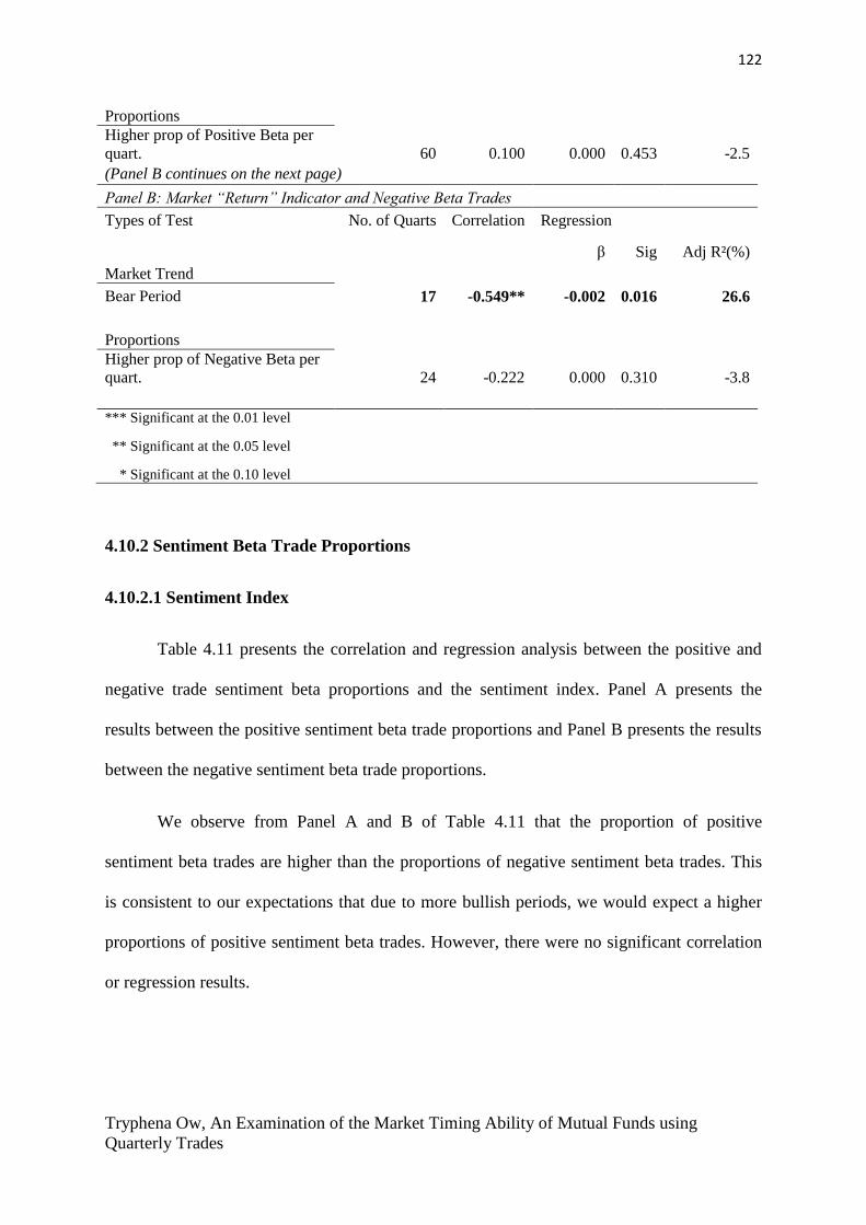
122
Tryphena Ow, An Examination of the Market Timing Ability of Mutual Funds using
Quarterly Trades
Proportions
Higher prop of Positive Beta per
quart. 60 0.100 0.000 0.453 -2.5
(Panel B continues on the next page)
Panel B: Market “Return” Indicator and Negative Beta Trades
Types of Test No. of Quarts Correlation Regression
β Sig Adj R²(%)
Market Trend
Bear Period 17 -0.549** -0.002 0.016 26.6
Proportions
Higher prop of Negative Beta per
quart. 24 -0.222 0.000 0.310 -3.8
*** Significant at the 0.01 level
** Significant at the 0.05 level
* Significant at the 0.10 level
4.10.2 Sentiment Beta Trade Proportions
4.10.2.1 Sentiment Index
Table 4.11 presents the correlation and regression analysis between the positive and
negative trade sentiment beta proportions and the sentiment index. Panel A presents the
results between the positive sentiment beta trade proportions and Panel B presents the results
between the negative sentiment beta trade proportions.
We observe from Panel A and B of Table 4.11 that the proportion of positive
sentiment beta trades are higher than the proportions of negative sentiment beta trades. This
is consistent to our expectations that due to more bullish periods, we would expect a higher
proportions of positive sentiment beta trades. However, there were no significant correlation
or regression results.

123
Tryphena Ow, An Examination of the Market Timing Ability of Mutual Funds using
Quarterly Trades
Table 4.11. Individual Correlation and Regression Analysis between Sentiment Beta Trades
(Proportions) and the Sentiment Index– June 1991 to March 2011
The different types of test based on the trade proportions are illustrated below. There are two types of
test: Market trend- Bull and Bear Market; Proportions of trades- Higher proportions in positive
sentiment beta trades and higher proportions in negative sentiment beta trades. Panel A presents the
results of the correlation and regression analysis between the positive sentiment beta trade proportions
and the Sentiment Index. Panel B presents the results of the correlation and regression analysis
between the negative sentiment beta trade proportions and the Sentiment Index. All regression
analysis are conducted individually. Regression equation: (ŷ= βₒ+β₁X1+εi); Dependent Variables:
Positive and Negative Trade Proportions; Independent Variable: Sentiment Index
Panel A: Sentiment Index and Positive Sentiment Beta Trades
Types of Test No. of Quarts Correlation Regression
β Sig Adj R²(%)
Market Trend
Bull Period 70 -0.051 -0.012 0.672 -1.2
Proportions
Higher prop of Positive Sen Beta
per quart. 55 0.03 0.004 0.827 -1.8
Panel B: Sentiment Index and Negative Sentiment Beta Trades
Types of Test No. of Quarts Correlation Regression
β Sig Adj R²(%)
Market Trend
Bear Period 17 -0.139 -0.013 0.594 -4.6
Proportions
Higher prop of Negative Sen Beta
per quart. 25 -0.197 -0.018 0.346 -0.3
*** Significant at the 0.01 level
** Significant at the 0.05 level
* Significant at the 0.10 level
4.10.2.2 Sentiment “Return” Indicator
Table 4.12 presents the correlation and regression analysis between the positive and
negative sentiment beta trade proportions and the sentiment “return” indicator. Panel A

124
Tryphena Ow, An Examination of the Market Timing Ability of Mutual Funds using
Quarterly Trades
presents the results between the positive sentiment beta trade proportions and Panel B
presents the results between the negative sentiment beta trade proportions.
Similar to Table 4.11, we observe from Panel A and B of Table 4.12 that the
proportions of positive sentiment beta trades are higher than the proportions of negative
sentiment beta trades. This is consistent to our expectations that due to more bullish periods,
we would expect a higher proportion of positive sentiment beta trades.
The results from Table 4.12 are consistent to our expectations that “return” indicators
would reflect more significant results as they capture standardized changes in each quarter
period. We observe from Panel A of Table 4.12 that the positive sentiment beta proportions
are lowly negatively correlated to the sentiment “return” indicator during bullish periods.
Although we expect that during bullish markets, there would be a higher proportion of
positive sentiment beta trades due to higher returns, results suggest an inverse relationship.
The correlation value was -0.299 with a significant level of 0.05. The beta coefficient
between the positive sentiment beta trade proportions and the sentiment “return” indicator is -
0.003 and it is significant at the 0.05 level. Having a beta coefficient of -0.003 implies that
for every 1 unit decrease in the sentiment “return” indicator, the positive sentiment beta trade
proportions will decrease by 0.003.The adjusted R2 value tells us that 7.6% of the positive
sentiment beta trade proportions can be explained by the sentiment “return” indicator during
bullish market periods.
We observe from Panel B of Table 4.12 that there is a highly positive correlation
between the negative sentiment trade proportions and the sentiment “return” indicator when
there is a higher proportion of negative sentiment trade proportions. This is consistent to our
expectations that during periods with higher proportion of negative sentiment trade
proportions, fund managers have anticipated a bearish market therefore shifted their

125
Tryphena Ow, An Examination of the Market Timing Ability of Mutual Funds using
Quarterly Trades
portfolios towards negative sentiment trade proportions. When the sentiment index reflects
poor market performance, there implies lower sentiment “returns”, therefore we expect fund
managers to tilt towards negative sentiment beta trade proportions. The correlation between
the negative sentiment beta trade proportions and the sentiment “return” indicator exhibited a
high correlation value of 0.698 and it is significant at the 0.01 level. The beta coefficient
between the negative sentiment beta trade proportions and the sentiment “return” indicator is
0.003 but however is not significant. The adjusted R2 value tells us that 46.5 % of the
negative sentiment beta trade proportions can be explained by the sentiment “return”
indicator.
Table 4.12. Individual Correlation and Regression Analysis between Sentiment Beta Trades
(Proportions) and the Sentiment “Return” Indicator– Jul 1991 to March 2011
The different types of test based on the trade proportions are illustrated below. There are two
types of test: Market trend- Bull and Bear Market; Proportions of trades- Higher proportions in
positive sentiment beta trades and higher proportions in negative sentiment beta trades. Panel A
presents the results of the correlation and regression analysis between the positive sentiment beta
trade proportions and the Sentiment “Return” Indicator. Panel B presents the results of the correlation
and regression analysis between the negative sentiment beta trade proportions and the Sentiment
“Return” Indicator. All regression analysis are conducted individually. Regression equation: (ŷ=
βₒ+β₁X1+εi); Dependent Variables: Positive and Negative Trade Proportions; Independent Variable:
Sentiment “Return” Indicator
Panel A: Sentiment “Return” Indicator and Positive Sentiment Beta Trades
Types of Test No. of Quarts Correlation Regression
β Sig Adj R²(%)
Market Trend
Bull Period 69 -0.299** -0.003 0.013 7.6
Proportions
Higher prop of Positive Sen Beta
per quart. 54 0.123 0.001 0.377 -0.4
Panel B: Sentiment “Return” Indicator and Negative Sentiment Beta Trades
Types of Test No. of Quarts Correlation Regression
β Sig Adj R²(%)
Market Trend
Bear Period 17 -0.264 -0.003 0.305 0.8
Proportions
Higher prop of Negative Sen Beta 25 0.698*** 0.003 0.000 46.5

126
Tryphena Ow, An Examination of the Market Timing Ability of Mutual Funds using
Quarterly Trades
per quart.
*** Significant at the 0.01 level
** Significant at the 0.05 level
* Significant at the 0.10 level
4.10.3 Momentum Trade Proportions
4.10.3.1 Momentum Index
Table 4.13 presents the correlation and regression analysis between the positive and
negative momentum trade proportions and the momentum index. Panel A presents the results
between the positive momentum trade proportions and Panel B presents the results between
the negative momentum trade proportions.
We observe from Panel A and B of Table 4.13 that the proportions of positive
momentum trades are lower than the proportions of negative momentum trades. This is
inconsistent to our expectations that due to more bullish periods, we would expect a higher
proportion of positive momentum trades. We consider how these mutual fund managers may
have pursued a contrarian strategy as mutual fund managers would buy funds that were past
“losers” and sell funds that were past “winners” based on their relative performance.
We observe from Panel A of Table 4.13 that the positive momentum trade proportions
are highly negatively correlated to the momentum index during bullish periods. Although we
expect that during bullish markets, there would be a higher proportion of positive momentum
trades due to the persistence in past “winners”, results suggest an inverse relationship. The
correlation value was -0.521 with a significant level of 0.01. The beta coefficient between the
positive momentum trade proportions and the momentum index is – 0.001 and it is significant
at the 0.01 level. Having a beta coefficient of -0.001 implies that for every 1 unit decrease in
the momentum index, the positive momentum trade proportions will decrease by 0.001.The

127
Tryphena Ow, An Examination of the Market Timing Ability of Mutual Funds using
Quarterly Trades
adjusted R2 value tells us that 24.0% of the positive momentum trade proportions can be
explained by the momentum index during bullish market periods.
From Panel A of Table 4.13, we observe that there is a highly negative correlation
between the positive momentum trade proportions and the momentum index when there is a
higher proportion of positive momentum trades. This is inconsistent to our expectations that
during periods with higher positive momentum trade proportions, fund managers have
anticipated a bullish market therefore shifted their portfolios towards positive momentum
trade proportions. When the values of the indicators are reflecting good market performance,
this implies a higher persistence on positive momentum trades, therefore a higher proportion
of positive momentum trades. The correlation between the positive momentum trade
proportions and the momentum index exhibited a high correlation value of 0.638 and it is
significant at the 0.05 level. The beta coefficient between the positive momentum trade
proportions and the momentum index is -0.001 and it is significant at the 0.05 level. Having a
beta coefficient of -0.001 implies that for every 1 unit decrease in the momentum index, the
positive momentum trade proportions will decrease by 0.001. The adjusted R2 value tells us
that 35.5 % of the positive momentum trade proportions can be explained by the momentum
index.
We also observe from Panel B of Table 4.13 that there is a high positive correlation
between the negative momentum trade proportions and the momentum index when there is a
higher proportion of negative momentum trades. This is consistent to our expectations that
during periods with higher negative momentum trade proportions, fund managers have
anticipated a bearish market therefore shifted their portfolios towards negative momentum
trade proportions. However, the correlation value, 0.546 was not significant. The beta
coefficient between the negative momentum trade proportions and the momentum index is
0.001 and it is significant at the 0.10 level. Having a beta coefficient of 0.001 implies that for
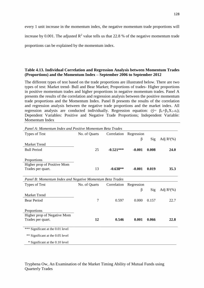
128
Tryphena Ow, An Examination of the Market Timing Ability of Mutual Funds using
Quarterly Trades
every 1 unit increase in the momentum index, the negative momentum trade proportions will
increase by 0.001. The adjusted R2 value tells us that 22.8 % of the negative momentum trade
proportions can be explained by the momentum index.
Table 4.13. Individual Correlation and Regression Analysis between Momentum Trades
(Proportions) and the Momentum Index – September 2006 to September 2012
The different types of test based on the trade proportions are illustrated below. There are two
types of test: Market trend- Bull and Bear Market; Proportions of trades- Higher proportions
in positive momentum trades and higher proportions in negative momentum trades. Panel A
presents the results of the correlation and regression analysis between the positive momentum
trade proportions and the Momentum Index. Panel B presents the results of the correlation
and regression analysis between the negative trade proportions and the market index. All
regression analysis are conducted individually. Regression equation: (ŷ= βₒ+β₁X1+εi);
Dependent Variables: Positive and Negative Trade Proportions; Independent Variable:
Momentum Index
Panel A: Momentum Index and Positive Momentum Beta Trades
Types of Test No. of Quarts Correlation Regression
β Sig Adj R²(%)
Market Trend
Bull Period 25 -0.521*** -0.001 0.008 24.0
Proportions
Higher prop of Positive Mom
Trades per quart. 13 -0.638** -0.001 0.019 35.3
Panel B: Momentum Index and Negative Momentum Beta Trades
Types of Test No. of Quarts Correlation Regression
β Sig Adj R²(%)
Market Trend
Bear Period 7 0.597 0.000 0.157 22.7
Proportions
Higher prop of Negative Mom
Trades per quart. 12 0.546 0.001 0.066 22.8
*** Significant at the 0.01 level
** Significant at the 0.05 level
* Significant at the 0.10 level

129
Tryphena Ow, An Examination of the Market Timing Ability of Mutual Funds using
Quarterly Trades
4.10.3.2 Momentum “Return” Indicator
Table 4.14 presents the correlation and regression analysis between the positive and
negative momentum trade proportions and the momentum “return” indicator. Panel A
presents the results between the positive momentum trade proportions and Panel B presents
the results between the negative momentum trade proportions.
Similar to Table 4.13, we observe from Panel A and B of Table 4.14 that the
proportion of positive momentum trades are lower than the proportion of negative momentum
trades. This is inconsistent to our expectations that due to more bullish periods, we would
expect a higher proportion of positive momentum trades. Although we expect the “return”
indicator to exhibit more significant results based on Table 4.14, the momentum index had
more significant correlation results. This reason may be cause by a pseudo return as the
momentum index is already considered as “return” indicator.
We observe from Panel B of Table 4.14 that the negative momentum trade
proportions are highly positively correlated to the momentum “return” indicator during
bearish periods. This is consistent to our expectations that during bearish periods, there would
be a higher proportion of negative momentum trades as the “returns” would be low. The
correlation value was -0.841 with a significant level of 0.01. The beta coefficient between the
negative momentum trade proportions and the momentum “return” indicator is 0.001 and it is
significant at the 0.05 level. Having a beta coefficient of 0.001 implies that for every 1 unit
increase in the momentum “return” indicator, the positive momentum beta proportions will
increase by 0.001.The adjusted R2 value tells us that 65.0% of the negative momentum trade
proportions can be explained by the momentum “return” indicator. However, the credibility
of these results are questionable as there were only 7 quarters.

130
Tryphena Ow, An Examination of the Market Timing Ability of Mutual Funds using
Quarterly Trades
Table 4.14. Individual Correlation and Regression Analysis between Momentum Trades
(Proportions) and the Momentum “Return” Indicator – October 2006 to September 2012
The different types of test based on the trade proportions are illustrated below. There are two
types of test: Market trend- Bull and Bear Market; Proportions of trades- Higher proportions in
positive momentum trades and higher proportions in negative momentum trades. Panel A
presents the results of the correlation and regression analysis between the positive momentum
trade proportions and the Momentum “Return” Indicator. Panel B presents the results of the
correlation and regression analysis between the negative trade proportions and the market index.
All regression analysis are conducted individually. Regression equation: (ŷ= βₒ+β₁X1+εi);
Dependent Variables: Positive and Negative Trade Proportions; Independent Variable:
Momentum “Return” Indicator
Panel A: Momentum “Return” Indicator and Positive Momentum Beta Trades
Types of Test No. of Quarts Correlation Regression
β Sig Adj R²(%)
Market Trend
Bull Period 20 -0.238 -0.001 0.313 0.4
Proportions
Higher prop of Positive
Mom Trades per quart. 13 -0.454 -0.001 0.119 13.4
Panel B: Momentum “Return” Indicator and Negative Momentum Beta Trades
Types of Test No. of Quarts Correlation Regression
β Sig Adj R²(%)
Market Trend
Bear Period 7 0.841** 0.001 0.018 65.0
Proportions
Higher prop of Negative
Mom Trades per quart. 11 -0.011 ~-0.000 0.974 -11.1 *** Significant at the 0.01 level
** Significant at the 0.05 level
* Significant at the 0.10 level
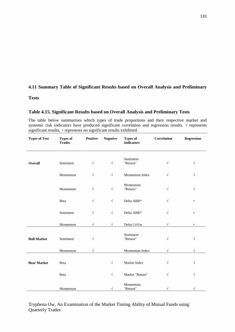
131
Tryphena Ow, An Examination of the Market Timing Ability of Mutual Funds using
Quarterly Trades
4.11 Summary Table of Significant Results based on Overall Analysis and Preliminary
Tests
Table 4.15. Significant Results based on Overall Analysis and Preliminary Tests
The table below summarises which types of trade proportions and their respective market and
systemic risk indicators have produced significant correlation and regression results. √ represents
significant results, × represents no significant results exhibited.
Types of Test
Types of
Trades
Positive Negative Types of
Indicators
Correlation Regression
Overall Sentiment √ √
Sentiment
"Return" √ √
Momentum √ √ Momentum Index √ √
Momentum √ √
Momentum
"Return" √ √
Beta √ √ Delta ABR* √ ×
Sentiment √ √ Delta ABR* √ ×
Momentum √ √ Delta CoVar √ ×
Bull Market Sentiment √
Sentiment
"Return" √ √
Momentum √ Momentum Index √ √
Bear Market Beta
√ Market Index √ √
Beta
√ Market "Return" √ √
Momentum √
Momentum
"Return" √ √

132
Tryphena Ow, An Examination of the Market Timing Ability of Mutual Funds using
Quarterly Trades
Higher Pos Prop. Momentum √
Momentum Index √ √
Higher Neg
Prop. Sentiment
√
Sentiment
"Return" √ √
Momentum √ Momentum Index √ √
* ABR: Absorption Ratio
4.12 Conclusion of Results and Discussion
By examining the proportions of statistically significant trades that encompass beta,
sentiment beta and momentum, we identify fund managers that adjust their portfolios
between positive and negative trade proportions in accordance to the market performance.
We refer this portfolio tilting action as the ability to time to the market. We evaluate trade
proportions as they provide insights on the direction that the mutual fund manager is
pursuing. Typically, when the market is performing well, we expect more positive trade
proportions in each quarter. In contrast, when the market is performing poorly, we expect
more negative trade proportions in each quarter.
Market and systemic risk indicators are important for our study as they reflect the
performance of the market and the economy. Market indicators are very important as they
reflect bearish and bullish market periods. Based on the index values, mutual fund managers
can shift their portfolios accordingly to take advantage of the market. We also created
“return” indicators to measure standardize changes in the index values in each quarter, this
helps to prevent spurious issues. After the recent global financial crisis, systemic risk
indicators were created to detect upcoming recession periods. We examined if these
statistically significant trades proportions have a direct relationship with these index values
during different market trends.

133
Tryphena Ow, An Examination of the Market Timing Ability of Mutual Funds using
Quarterly Trades
We conducted an overall correlation and regression analysis to investigate in general,
if there were any significant relationship between the statistically significant trade
proportions and their respective indicators. Beta trade proportions were examined with the
values of the market index, market “return” indicator and the systemic risk indicators.
Sentiment beta trade proportions were examined with the values of the sentiment index,
sentiment “return” indicator and the systemic risk indicators. Momentum trade proportions
were examined with the values of the momentum index, momentum “return” indicator and
the systemic risk indicators.
Our results showed that only positive sentiment trade proportions and positive
momentum trade proportions displayed significant correlation and regression results between
their respective indicators. However, these positive trade proportions exhibited an inverse
relationship. This suggests the possibility of a contrarian strategy.
Preliminary tests were also conducted with the consideration of bullish and bearish
market trends as well as periods with higher proportions of positive or negative trade
proportions. These test are conducted to investigate if mutual fund managers are selective in
adjusting their portfolios based on certain conditions.
For bullish market trends, we observe significant correlation and regression results
between the positive sentiment trade proportions and the sentiment “return” indicator.
However, an inverse relationship was exhibited. The positive momentum trade proportions
also displayed significant correlation and regression results when evaluated against the
momentum index. Similarly, an inverse relationship was exhibited. For bearish market
trends, the negative beta exhibited significant correlation and regression results when
compared to the market index and the market “return” indicator. These results suggest an
134
Tryphena Ow, An Examination of the Market Timing Ability of Mutual Funds using
Quarterly Trades
inverse relationship. Results were also significant between negative momentum trade
proportions and the momentum “return” indicator with a positively high correlation value.
For periods with higher proportions of positive proportion trades, we expect that fund
managers had anticipated a bullish market therefore shifted their portfolios towards positive
trades. However, there was only one significant results between the positive momentum trade
proportion and the momentum index however, it was an inverse relationship. For the periods
with higher proportions of negative proportion trades, we expect that fund managers had
anticipated a bearish market therefore shifted their portfolios towards negative trades. The
analysis between the negative sentiment trade proportions and the sentiment “return”
indicator displayed a significant correlation and regression results with a high positive
correlation value. Although the analysis between the negative momentum trade proportions
and the momentum index displayed a high correlation value, it is not significant.
Based on these analyses, we observe mostly inverse relationship patterns between
these trade proportions and their respective indicators variables. However, beta trade
proportions did not reflect any substantial correlation or regression results. Similarly, the
results between the trade proportions and the systemic risk indicators were not constructive.
Some possible reasons could be that the variations of the dependent variables, statistically
significant trade proportions and the independent variables, market and systemic risk
indicators were not very high. We also consider how using statistically significant trade
proportions might have affected our results. Lastly, using proportions might lead to herding
behaviour providing inaccurate analyses.
We consider the possibility that these mutual fund managers were unable to select
turning points of bullish and bearish market periods. Therefore, we proceed to conduct robust

135
Tryphena Ow, An Examination of the Market Timing Ability of Mutual Funds using
Quarterly Trades
testing to identify if these managers are capable of identifying large or small market shocks
and market persistence.
CHAPTER 5
ROBUST TESTING
5.1 Introduction
This chapter shows the analyses and results of my robust tests. We conducted various
robust test; Magnitude of Change, Changes in Standard Deviation, Changes in Signs and
Persistence. We also conducted a multiple regression analysis to simultaneously test all
independent variables in our analysis to examine if one or more variables will affect the
predictability value of our dependent variable. Similar to the results of the preliminary tests,
sentiment beta and momentum trade proportions exhibited the most number of significant
results. However, both sentiment beta and momentum trade proportions exhibited an inverse
relationship with their respective indicators.
5.2 Overview of Robust Testing
In the previous chapter, we conducted an overall correlation and regression analysis
between the statistically significant trade proportions, market and systemic risk indicators. An
overall test does not take into consideration that these mutual fund managers may be selective

136
Tryphena Ow, An Examination of the Market Timing Ability of Mutual Funds using
Quarterly Trades
in adjusting their portfolios according to different situations of the market. This analysis
provides some general insights on the possibility of any form of direct or inverse relationship
between these statistically significant trade proportions, the market and systemic risk
indicators.
After conducting an overall analysis, we ran some preliminary tests between these
statistically trade proportions and their respective indicators. First, we consider if mutual fund
managers are capable of predicting bullish and bearish market trends. Second we examine if
there were any form of relationship between positive (negative) trade proportions and their
respective indicators when we isolated periods with higher proportions of positive (negative)
trade proportions. We expect that periods with high proportions of positive (negative) trades
are influence by good (poor) market performance which are reflected by the values of the
indicators. Based on the results, we observe an inverse relationships between positive
momentum trade proportions the momentum index. It is plausible that these mutual fund
managers are pursuing a contrarian strategy. We investigate further by conducting a few
robust tests between the trade proportions and their respective market indicators.
Robust testing is essential as it subjects the constructs to rigorous statistical testing,
thus ensuring the reliability of the results obtained. It is possible that fund managers may not
be able to isolate turning points in the market’s economic or financial behaviour but identify
or be sensitized to large market shocks, market persistence. We have considered four types of
robust test; Magnitude of change, Changes in Standard Deviation, Changes in Sign and
Persistence. We will examine these in turn.
Figure 5.1 provides a schematic diagram on the types of robust tests that we have
considered. The diagram presents which type of robust test will be conducted on the related
statistically significant trade proportions that encompass beta, sentiment beta and momentum.

137
Tryphena Ow, An Examination of the Market Timing Ability of Mutual Funds using
Quarterly Trades
Figure 5.1: Types of Robust Test Conducted
The figure below illustrates the overall process of robust testing. There are four types of robust tests.
(1) Magnitude of Change (2) Changes in Standard Deviation (3) Changes in Signs (4) Persistence.
Test (1) and (2) are mainly for “return” indicators. Beta trade proportions: Test (1), (2), (3) and (4);
Sentiment beta trade proportions: Test (3) and (4); Momentum trade proportions: Test (4)
Robust Test
Magnitude of
Change
(1)
Changes in
Standard Deviations
(2)
Changes in Signs
(3)
Persistence
(4)
Beta Trade
proportions
Beta Trade
Proportions
Beta Trade
proportions
Beta Trade
proportions
Market “Return”
Indicator
Market “Return”
Indicator
Market “Return”
Indicator
Market “Return”
Indicator
Sentiment beta
proportions
Sentiment beta
proportions

138
Tryphena Ow, An Examination of the Market Timing Ability of Mutual Funds using
Quarterly Trades
-Sentiment
“Return” indicator
-Sentiment
“Return” Indicator
-Sentiment Index
-Sentiment Index
Momentum
Proportions
-Momentum
“Return” Indicator
-Momentum Index
While these statistically significant trades proportions that encompass beta, sentiment
beta and momentum are directly related to the market index, sentiment index and momentum
index, emphasis is given to the market “return”, sentiment “return” and momentum “return”
indicators. We expect more significant results to be exhibited from these “return: indicators
as they are constructed to detect standardized changes in the index values against the base
values and this avoids spurious issues.
5.3 Beta Trade Proportions and the Market “Return” Indicator
5.3.1 Test (1): Magnitude of Change
The magnitude of change test allows us to identify if mutual fund managers had
successful trade-offs. We examine if they are capable of selecting either large or small
changes based on the market “returns” to adjust their portfolios to take advantage of the
market. Big changes are market returns that are above 5%, 10%, 15%, 20%, 25% and 30%
and small changes are market returns that are lower than -5%, -10%, -15%, -20%, -25% and -
30%.

139
Tryphena Ow, An Examination of the Market Timing Ability of Mutual Funds using
Quarterly Trades
Table 5.1 presents the number of quarter observations based on their returns. This
provides some understanding on the direction that these mutual fund managers were
pursuing. We expect that during periods with higher returns, mutual fund managers will be
tilting their portfolios towards positive beta trade proportions. Similarly we expect that during
periods with lower returns, mutual fund managers will be tilting their portfolios towards
negative beta trade proportions. High returns are related to bullish market periods and low
returns are related to bearish market periods.
Table 5.1. Number of quarters in relation to Market “Returns”- July 1991 to September
2012
Column 2 presents the number of quarters that have market return above 5%, 10%, 15%. 20%. 25%
and 30%. Column 4 presents the number of quarters that have market returns less than -5%, -10%, -
15%, -20%, -25% and -30%.
Returns Above No. of Quarts Returns Below No. if Quarts Total No. of Quarts
30% 19 -30% 12 31
25% 22 -25% 13 35
20% 30 -20% 13 43
15% 38 -15% 15 53
10% 41 -10% 22 63
5% 53 -5% 23 76
We observe from Table 5.1 that between 1991 and 2012, most market “returns” were
more than 5%. There were 53 quarter observations that reflected market returns that were
above 5%. However, 5% change may not be significant enough to detect the market timing
abilities of the mutual fund managers.
Logan (2014) reported that that a bull market period occurs when the index is rising
20% off the bear market low and a bear market period occurs when the index is falling 20%
off the bull market. Therefore, we expect mutual fund managers to display market timing
abilities during quarters with returns higher than 20% and returns lower than -20%.

140
Tryphena Ow, An Examination of the Market Timing Ability of Mutual Funds using
Quarterly Trades
5.3.2 Test (2): Changes in standard deviation
Similar to the test of magnitude of changes, we evaluate how confident fund managers
are in picking changes. We examine market returns that are above the mean plus half a
standard deviation and market returns that are below the mean minus half a standard
deviation. We expect mutual fund managers to tilt their portfolios towards positive beta trade
proportions when returns are above the mean plus half a standard deviation and we expect
mutual fund managers to tilt their portfolios towards negative beta trade proportions when
returns are below the mean plus half a standard deviation. There is a 38% chance that the
mutual fund managers will select positive trade proportions when returns are above the mean
and a 38% chance that the mutual fund managers will select negative trade proportions when
returns are below the mean.
Table 5.2. Empirical Rule for Normally Distributed Data
Distance from mean Values within distance
𝜇 ± 0.5𝜎 38%
𝜇 ± 1𝜎 68%
𝜇 ± 2𝜎 95%
𝜇 ± 3𝜎 99.7%
Source: Black et al. (2016)
5.3.3 Test (3): Changes in Signs
We examine if mutual fund managers are capable of selecting turning points in the
values of the market “return” indicator. We expect successful market timers to tilt their
portfolios towards positive trade proportions when market “returns” transit from negative to
positive value from the previous quarter. This could be a signal of a bull market period.
Similarly, we expect successful market timers to tilt their portfolios towards negative trade
141
Tryphena Ow, An Examination of the Market Timing Ability of Mutual Funds using
Quarterly Trades
proportions when market “returns” transit from positive to negative values from the previous
quarter. This could be a signal of a bear market period.
5.3.4 Test (4): Persistence in Index
We examine if mutual fund managers exhibit market timing abilities based on market
persistence. We expect mutual fund managers to tilt their portfolios towards positive beta
trade proportions when the market “returns” displays consecutive increases in values.
Similarly, we expect mutual fund managers to tilt their portfolios towards negative beta trade
proportions when the market “returns” displays consecutive decreases in values. Market
persistence is similar to momentum strategies with the belief that past “winners” are still
“winners” and past “losers” are still “losers”. We also observed the market “return” indicator
has exhibited more than three quarters of consecutive decreases in “returns”.
Table 5.3 presents the correlation and regression results of the robust test that we have
conducted between the proportions of negative, positive beta trades and the market “return”
indicator. Panel A presents the results from the magnitude of change test. Panel B presents
the results from the changes in standard deviation test. Panel C presents the results from the
changes in signs test. Panel D presents the results from the market persistence test.
We observe from Panel A (Magnitude of Changes) and Panel B (Changes in Standard
Deviation) of Table 5.3 that there were no significant correlation or regression results.
From Panel C (Changes in Signs) of Table 5.3, we observe significant results
between the negative beta trade proportions and the market “return” indicator. Although there
were no significant correlations, the correlation value of -0.346 suggests an inverse
relationship. This is inconsistent to our expectations that mutual fund managers will tilt their
portfolios towards negative trade proportions when the “return” values transit from a positive
“return” to a negative “return”, a possible signal of a bearish market. The beta coefficient

142
Tryphena Ow, An Examination of the Market Timing Ability of Mutual Funds using
Quarterly Trades
between the negative beta trade proportions and the market “return” index is -0.001,
significant at the 0.10 level. Having a beta coefficient of -0.001 implies that for every 1 unit
decrease in the market “return” indicator, the negative beta trade proportions will decrease by
0.001. The adjusted R2 value tells us that 8.6% of the negative beta trade proportions can be
explained by the market “return” indicator.
We observe from Panel D (Persistence) of Table 5.3 that the negative beta trade
proportions exhibited significant regression results when the market displayed consecutive
decreases in “returns”. Although there were no significant correlation results, the value -
0.274 suggests an inverse relationship. The beta coefficient between the negative beta trade
proportions and the market “return” index is -0.001, significant at the 0.10 level. Having a
beta coefficient of -0.001 implies that for every 1 unit decrease in the market “return”
indicator, the negative beta trade proportions will decrease by 0.001. The adjusted R2 value
tells us that 5.5% of the negative beta trade proportions can be explained by the market
“return” indicator.
Table 5.3. Robust Testing between Proportions of Beta Trades based and the Market “Return” Indicator
The different types of test conducted between the positive and negative proportion of trade betas and the market
“return” indicator are illustrated below. There are four types of robust test: Magnitude of change based on
market “returns”; Changes in standard deviation of market “returns”- Market “return” > Mean+0.5SD and
Market “return” < Mean-0.5SD; Changes in sign based on the positive or negative index value per quarter;
Persistence in positive or negative signs of values in the index per quarter. Panel A presents the correlation and
regression results of the magnitude of changes test. Panel B presents the correlation and regression results of the
changes in standard deviation test. Panel C presents the correlation and regression results of the changes in signs
test. Panel D presents the correlation and regression results of the persistence test. There were only three or
more consecutive decrease in the values of the market “return” indicator, there were no three or more
consecutive increases. Simple regression analysis are conducted. (ŷ=βₒ+β₁X1+εi). DV: positive or negative trade
proportions; IV: Market “Return” Indicator.
Types of Test No. of Quarts Correlation Regression
β Sig Adj R²(%)
Panel A: Magnitude of Change (Jul 1991 - Sep 2012)
Market Return > 30% 15 -0.192 -0.001 0.494 -3.7
Market Return < -30% 9 -0.455 -0.002 0.219 9.3
Market Return > 25% 22 -0.241 -0.001 0.281 1.1
Market Return < -25% 10 -0.427 -0.002 0.218 8.0
Market Return >20% 29 -0.125 -0.001 0.520 -2.1
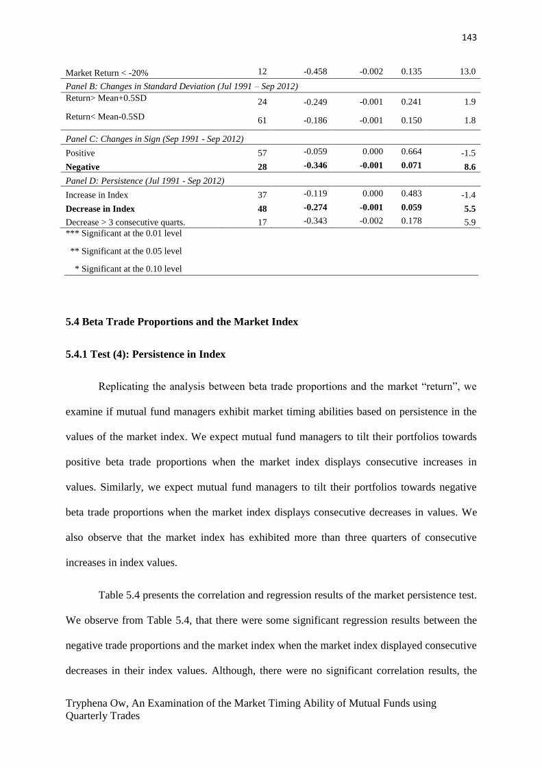
143
Tryphena Ow, An Examination of the Market Timing Ability of Mutual Funds using
Quarterly Trades
Market Return < -20% 12 -0.458 -0.002 0.135 13.0
Panel B: Changes in Standard Deviation (Jul 1991 – Sep 2012)
Return> Mean+0.5SD 24 -0.249 -0.001 0.241 1.9
Return< Mean-0.5SD 61 -0.186 -0.001 0.150 1.8
Panel C: Changes in Sign (Sep 1991 - Sep 2012)
Positive 57 -0.059 0.000 0.664 -1.5
Negative 28 -0.346 -0.001 0.071 8.6
Panel D: Persistence (Jul 1991 - Sep 2012)
Increase in Index 37 -0.119 0.000 0.483 -1.4
Decrease in Index 48 -0.274 -0.001 0.059 5.5
Decrease > 3 consecutive quarts. 17 -0.343 -0.002 0.178 5.9
*** Significant at the 0.01 level
** Significant at the 0.05 level
* Significant at the 0.10 level
5.4 Beta Trade Proportions and the Market Index
5.4.1 Test (4): Persistence in Index
Replicating the analysis between beta trade proportions and the market “return”, we
examine if mutual fund managers exhibit market timing abilities based on persistence in the
values of the market index. We expect mutual fund managers to tilt their portfolios towards
positive beta trade proportions when the market index displays consecutive increases in
values. Similarly, we expect mutual fund managers to tilt their portfolios towards negative
beta trade proportions when the market index displays consecutive decreases in values. We
also observe that the market index has exhibited more than three quarters of consecutive
increases in index values.
Table 5.4 presents the correlation and regression results of the market persistence test.
We observe from Table 5.4, that there were some significant regression results between the
negative trade proportions and the market index when the market index displayed consecutive
decreases in their index values. Although, there were no significant correlation results, the
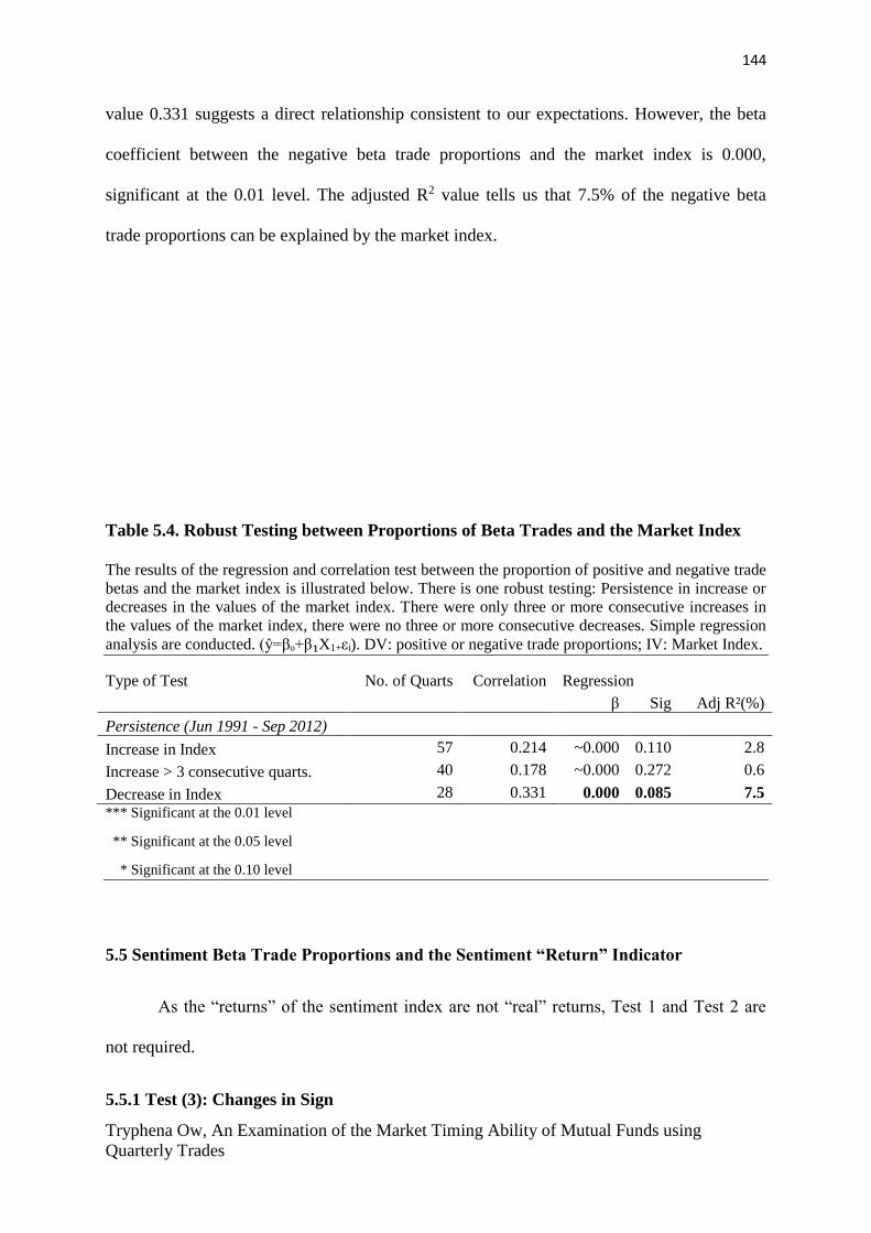
144
Tryphena Ow, An Examination of the Market Timing Ability of Mutual Funds using
Quarterly Trades
value 0.331 suggests a direct relationship consistent to our expectations. However, the beta
coefficient between the negative beta trade proportions and the market index is 0.000,
significant at the 0.01 level. The adjusted R2 value tells us that 7.5% of the negative beta
trade proportions can be explained by the market index.
Table 5.4. Robust Testing between Proportions of Beta Trades and the Market Index
The results of the regression and correlation test between the proportion of positive and negative trade
betas and the market index is illustrated below. There is one robust testing: Persistence in increase or
decreases in the values of the market index. There were only three or more consecutive increases in
the values of the market index, there were no three or more consecutive decreases. Simple regression
analysis are conducted. (ŷ=βₒ+β₁X1+εi). DV: positive or negative trade proportions; IV: Market Index.
Type of Test No. of Quarts Correlation Regression
β Sig Adj R²(%)
Persistence (Jun 1991 - Sep 2012) Increase in Index 57 0.214 ~0.000 0.110 2.8
Increase > 3 consecutive quarts. 40 0.178 ~0.000 0.272 0.6
Decrease in Index 28 0.331 0.000 0.085 7.5
*** Significant at the 0.01 level
** Significant at the 0.05 level
* Significant at the 0.10 level
5.5 Sentiment Beta Trade Proportions and the Sentiment “Return” Indicator
As the “returns” of the sentiment index are not “real” returns, Test 1 and Test 2 are
not required.
5.5.1 Test (3): Changes in Sign

145
Tryphena Ow, An Examination of the Market Timing Ability of Mutual Funds using
Quarterly Trades
We examine if mutual fund managers are capable of selecting turning points in the
values of the sentiment “return” indicator. We expect successful market timers to tilt their
portfolios towards positive sentiment beta trade proportions when sentiment “returns” transit
from negative to a positive value from the previous quarter. It is plausible that the investor’s
sentiment has increased when the market is performing well. Similarly, we expect successful
market timers to tilt their portfolios towards negative sentiment trade proportions when
sentiment “returns” transit from positive to negative values from the previous quarter. It is
likely that the investor’s sentiment has decreased when the market is performing poorly.
5.5.2 Test (4): Persistence in Index
We examine if mutual fund managers exhibit market timing abilities based on
sentiment persistence. We expect mutual fund managers to tilt their portfolios towards
positive sentiment beta trade proportions when the sentiment “returns” displays consecutive
increases in values. When returns are “high”, it suggest that an investor’s sentiment is high.
An investor’s sentiment is usually high when the market is performing well. Similarly, we
expect mutual fund managers to tilt their portfolios towards negative sentiment beta trade
proportions when the sentiment “returns” displays consecutive decreases in values. When
“returns” are low, it suggest that an investor’s sentiment is low. An investor’s sentiment is
usually low when the market is performing badly. We also observed the sentiment “return”
indicator has exhibited more than three quarters of consecutive decreases in “returns”.
Table 5.5 presents the correlation and regression results of the robust test that we have
conducted between the proportions of negative, positive sentiment beta trades and the
sentiment “return” indicator. Panel A presents the results from the changes in signs test. Panel
B presents the results from the market persistence test.

146
Tryphena Ow, An Examination of the Market Timing Ability of Mutual Funds using
Quarterly Trades
We observe from Panel A (Changes in Signs) of Table 5.5 that there were some
significant results between the positive sentiment beta trade proportions and the sentiment
“return” indicator. The correlation value of -0.428 is significant at the 0.01 level, this
suggests an inverse relationship. This result is inconsistent to our expectations that mutual
fund managers will tilt their portfolios towards positive trade proportions when the “return”
values transit from a positive “return” to a negative “return”, a possible signal of a bullish
market. The beta coefficient between the sentiment beta trade proportions and the sentiment
“return” index is -0.005, significant at the 0.01 level. Having a beta coefficient of -0.005
implies that for every 1 unit decrease in the sentiment “return” indicator, the positive
sentiment beta trade proportions will decrease by 0.005. The adjusted R2 value tells us that
16.1% of the positive sentiment beta trade proportions can be explained by the sentiment
“return” indicator.
We observe from Panel D (Persistence) of Table 5.5 that the positive sentiment beta
trade proportions exhibited some significant regression results when the sentiment index
displayed consecutive increase in “returns”. The correlation value of -0.423 significant at the
0.05 level suggests an inverse relationship. This is inconsistent to our expectations that
mutual fund managers will tilt their portfolios towards positive trade proportions when the
“return” values consecutively increase in each quarter which suggest that the market is
performing well. The beta coefficient between the sentiment beta trade proportions and the
sentiment “return” index is -0.005, significant at the 0.05 level. Having a beta coefficient of -
0.005 implies that for every 1 unit decrease in the sentiment “return” indicator, the positive
sentiment beta trade proportions will decrease by 0.005. The adjusted R2 value tells us that
15.4% of the positive sentiment beta trade proportions can be explained by the sentiment
“return” indicator.
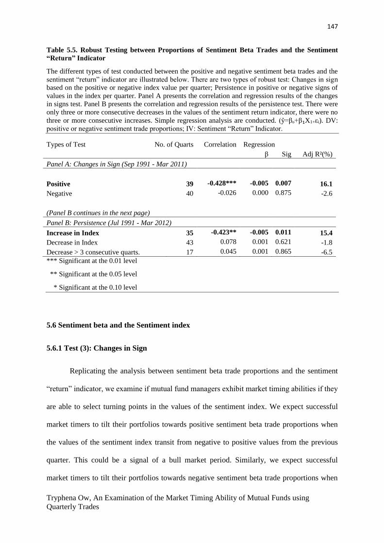
147
Tryphena Ow, An Examination of the Market Timing Ability of Mutual Funds using
Quarterly Trades
Table 5.5. Robust Testing between Proportions of Sentiment Beta Trades and the Sentiment
“Return” Indicator
The different types of test conducted between the positive and negative sentiment beta trades and the
sentiment “return” indicator are illustrated below. There are two types of robust test: Changes in sign
based on the positive or negative index value per quarter; Persistence in positive or negative signs of
values in the index per quarter. Panel A presents the correlation and regression results of the changes
in signs test. Panel B presents the correlation and regression results of the persistence test. There were
only three or more consecutive decreases in the values of the sentiment return indicator, there were no
three or more consecutive increases. Simple regression analysis are conducted. (ŷ=βₒ+β₁X1+εi). DV:
positive or negative sentiment trade proportions; IV: Sentiment “Return” Indicator.
Types of Test No. of Quarts Correlation Regression
β Sig Adj R²(%)
Panel A: Changes in Sign (Sep 1991 - Mar 2011)
Positive 39 -0.428*** -0.005 0.007 16.1
Negative 40 -0.026 0.000 0.875 -2.6
(Panel B continues in the next page)
Panel B: Persistence (Jul 1991 - Mar 2012)
Increase in Index 35 -0.423** -0.005 0.011 15.4
Decrease in Index 43 0.078 0.001 0.621 -1.8
Decrease > 3 consecutive quarts. 17 0.045 0.001 0.865 -6.5
*** Significant at the 0.01 level
** Significant at the 0.05 level
* Significant at the 0.10 level
5.6 Sentiment beta and the Sentiment index
5.6.1 Test (3): Changes in Sign
Replicating the analysis between sentiment beta trade proportions and the sentiment
“return” indicator, we examine if mutual fund managers exhibit market timing abilities if they
are able to select turning points in the values of the sentiment index. We expect successful
market timers to tilt their portfolios towards positive sentiment beta trade proportions when
the values of the sentiment index transit from negative to positive values from the previous
quarter. This could be a signal of a bull market period. Similarly, we expect successful
market timers to tilt their portfolios towards negative sentiment beta trade proportions when

148
Tryphena Ow, An Examination of the Market Timing Ability of Mutual Funds using
Quarterly Trades
the values of the sentiment index transit from positive to negative values from the previous
quarter. This could be a signal of a bear market period. Sentiment values are usually high
during a bullish market period and low during a bearish market period.
5.6.2 Test (4): Persistence in Index
Similarly, we replicate the analysis between sentiment beta trade proportions and the
sentiment “return” indicator, we examine if mutual fund managers exhibit market timing
abilities based on sentiment persistence. We expect mutual fund managers to tilt their
portfolios towards positive sentiment beta trade proportions when the sentiment index
displays consecutive increases in values. When an investor’ sentiment is high, this suggest
that the market is performing well. Similarly, we expect mutual fund managers to tilt their
portfolios towards negative sentiment beta trade proportions when the sentiment index
displays consecutive decreases in values. When an investor’ sentiment is low, this suggest
that the market is performing poorly. We also observe that the sentiment index has exhibited
more than three quarters of consecutive increases as well as decreases in their index values.
Table 5.6 presents the correlation and regression results of the robust test that we have
conducted between the proportions of negative, positive sentiment beta trades and the
sentiment index. Panel A presents the results from the changes in signs test. Panel B presents
the results from the sentiment persistence test. However, there were significant correlation or
regression results.
Table 5.6. Robust Testing between Proportions of Sentiment Beta Trades and Sentiment
Index
The different types of test conducted between the positive and negative proportion of sentiment beta
trades and the Sentiment index are illustrated below. There are two types of robust test: Changes in
sign based on the positive and negative values of the sentiment index per quarter; Persistence in
positive and negative signs of values in the index per quarter. Panel A presents the correlation and
regression results of changes in signs test. Panel B presents the correlation and regression results of
persistence test. All regression analysis are conducted individually. There were three or more
consecutive increases and decreases in the values of the sentiment index. Simple regression analysis
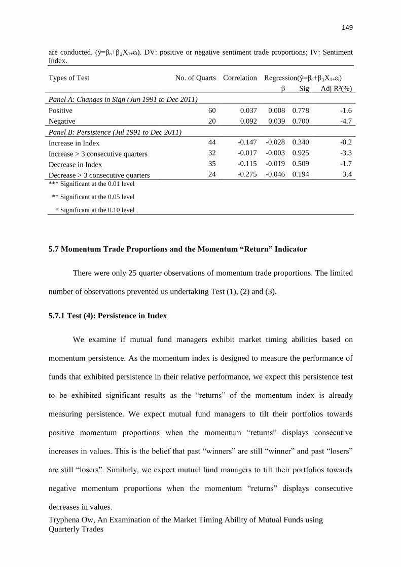
149
Tryphena Ow, An Examination of the Market Timing Ability of Mutual Funds using
Quarterly Trades
are conducted. (ŷ=βₒ+β₁X1+εi). DV: positive or negative sentiment trade proportions; IV: Sentiment
Index.
Types of Test No. of Quarts Correlation Regression(ŷ=βₒ+β₁X1+εi)
β Sig Adj R²(%)
Panel A: Changes in Sign (Jun 1991 to Dec 2011)
Positive 60 0.037 0.008 0.778 -1.6
Negative 20 0.092 0.039 0.700 -4.7
Panel B: Persistence (Jul 1991 to Dec 2011)
Increase in Index 44 -0.147 -0.028 0.340 -0.2
Increase > 3 consecutive quarters 32 -0.017 -0.003 0.925 -3.3
Decrease in Index 35 -0.115 -0.019 0.509 -1.7
Decrease > 3 consecutive quarters 24 -0.275 -0.046 0.194 3.4
*** Significant at the 0.01 level
** Significant at the 0.05 level
* Significant at the 0.10 level
5.7 Momentum Trade Proportions and the Momentum “Return” Indicator
There were only 25 quarter observations of momentum trade proportions. The limited
number of observations prevented us undertaking Test (1), (2) and (3).
5.7.1 Test (4): Persistence in Index
We examine if mutual fund managers exhibit market timing abilities based on
momentum persistence. As the momentum index is designed to measure the performance of
funds that exhibited persistence in their relative performance, we expect this persistence test
to be exhibited significant results as the “returns” of the momentum index is already
measuring persistence. We expect mutual fund managers to tilt their portfolios towards
positive momentum proportions when the momentum “returns” displays consecutive
increases in values. This is the belief that past “winners” are still “winner” and past “losers”
are still “losers”. Similarly, we expect mutual fund managers to tilt their portfolios towards
negative momentum proportions when the momentum “returns” displays consecutive
decreases in values.

150
Tryphena Ow, An Examination of the Market Timing Ability of Mutual Funds using
Quarterly Trades
Table 5.7 presents the correlation and regression results of the persistence robust test
that we have conducted between the proportions of negative, positive momentum trades and
the momentum “return” indicator. We observe from Table 5.7 that despite no significant
correlation results between the negative momentum proportions and the momentum “return”
indicator when the momentum indicator displayed consecutive decreases in “returns”. The
correlation value, 0.571 suggests a direct relationship which is consistent to our expectations.
The beta coefficient between the negative beta trade proportions and the momentum “return”
index is 0.001, significant at the 0.10 level. Having a beta coefficient of 0.001 implies that for
every 1 unit increase in the momentum “return” indicator, the negative momentum trade
proportions will increase by 0.001. The adjusted R2 value tells us that 25.8% of the negative
beta trade proportions can be explained by the momentum “return” indicator.
Table 5.7. Robust Testing between Proportions of Momentum Trades and the
Momentum “Return” Indicator
The robust test between the positive and negative proportions of trades and the momentum “return”
indicator are illustrated below. Table 5.7 presents the correlation and regression results of the
persistence test. There were no consecutive increases or decrease in momentum return indicator.
Simple regression analysis are conducted. (ŷ=βₒ+β₁X1+εi). DV: positive or negative momentum trade
proportions; IV: Momentum “Return” Indicator.
Types of Test No. of Quarts Correlation Regression
β Sig Adj R²(%)
Panel D: Persistence (Oct 2006 - Sep 2006)
Increase in Index 11 0.028 0.000 0.934 -11.0
Decrease in Index 12 0.571 0.001 0.053 25.8 *** Significant at the 0.01 level
** Significant at the 0.05 level
* Significant at the 0.10 level
5.8 Momentum Trade Proportions and the Momentum Index
5.8.1 Test (4): Persistence in Index
Replicating the analysis between momentum trade proportions and the momentum
“return” indicator, we examine if mutual fund managers exhibit market timing abilities based

151
Tryphena Ow, An Examination of the Market Timing Ability of Mutual Funds using
Quarterly Trades
on persistence in the values of the momentum index. We expect mutual fund managers to tilt
their portfolios towards positive momentum proportions when the momentum index displays
consecutive increases in values. Similarly, we expect mutual fund managers to tilt their
portfolios towards negative momentum proportions when the momentum index displays
consecutive decreases in values.
Table 5.8 presents the correlation and regression results of the persistence robust test
that we have conducted between the proportions of negative, positive momentum trades and
the momentum index. We observe from Table 5.8 that the positive momentum trade
proportions exhibited some significant regression results when the values of the momentum
index displayed consecutive increases in values. The correlation value of -0.552, significant
at the 0.05 level suggests an inverse relationship. Inconsistent to our expectations that mutual
fund managers will tilt their portfolios towards positive momentum trade proportions when
the index values consecutively increase in each quarter which suggest that the persistence
level is high implying that the market is performing well. The beta coefficient between the
momentum trade proportions and the momentum index is -0.001, significant at the 0.05 level.
Having a beta coefficient of -0.001 implies that for every 1 unit decrease in the momentum
index, the positive momentum trade proportions will decrease by 0.001. The adjusted R2
value tells us that 25.1% of the positive momentum trade proportions can be explained by the
momentum index.
Although the results from Table 5.8, suggest the possibility of a contrarian strategy,
based on the results of Table 5.7, there were no inverse relationships between the momentum
trade proportions and the momentum “return” indicator. However, results may be misleading
as the momentum index is already considered as a “return” indicator. Having a “return” on
“return” analysis may lead to inconsistent results due to pseudo returns.

152
Tryphena Ow, An Examination of the Market Timing Ability of Mutual Funds using
Quarterly Trades
Table 5.8. Robust Testing between Proportions of Momentum Trades and the
Momentum Index
The robust test between the positive and negative proportions of trades and the momentum index are
illustrated below. Table 7 presents the correlation and regression results of the persistence test. There
were no consecutive increases or decrease in momentum return indicator. Simple regression analysis
are conducted. (ŷ=βₒ+β₁X1+εi). DV: Positive or negative momentum trade proportions; IV:
Momentum Index.
Types of Test No. of Quarts Correlation Regression (ŷ= βₒ+β₁X1+εi)
β Sig Adj R²(%)
Persistence (Sep 2006 - Sep 2012)
Increase in Index 15 -0.552** -0.001 0.033 25.1
Decrease in Index 9 -0.286 0.000 0.456 -5.0
*** Significant at the 0.01 level
** Significant at the 0.05 level
* Significant at the 0.10 level
5.9 Multiple Regression Analysis
In the previous chapter, we conducted simple regression analysis between the trade
proportions and their respective market and systemic indicators. However to our dismay, we
did not find any exceptional results. We considered an alternative analysis by conducting a
multiple regression analysis.
We consider how two or more independent variables will affect the predictability
value of the dependent variable. For example, we examine how the market index as well as
how each individual component of the systemic risk indicator will simultaneously affect the
regression results when run in a multiple regression model, unlike the simple regression
model which concentrates on how the market index or the Absorption ratio influences the
trade proportions of the market beta individually.
The multiple regression analysis is conducted using the stepwise method. Stepwise
linear regression is the best option as it regresses multiple independent variables while
concurrently removing variables that are not important. Multiple regression analysis are

153
Tryphena Ow, An Examination of the Market Timing Ability of Mutual Funds using
Quarterly Trades
conducted on a step by step basis, each time excluding variables have the weakest correlation
leaving the best independent variable that best explain the distribution.
5.9.1 Market Beta
5.9.1.1 Positive Market Beta Proportions with the Market “Return” Indicator
The dependent variable of this multiple regression model is the positive proportions of
beta trades. The independent variables of this multiple regression model are the market
“return” indicator, and 11 of the systemic risk indicators. They are the Absorption Ratio,
Delta Absorption Ratio, AIM, CoVar, Delta CoVar, Book Leverage, Market Leverage, Real
Volatility, Turbulence, CATFIN and PQR indicators.
We have presented the stepwise regression results of positive beta proportions as the
results of the negative beta proportions are the same but in opposite signs. The emphasize is
on the positive beta trade proportions as there are more bullish market periods than bearish
market periods. We expect a higher proportion of positive beta trades.
We observe from Table 5.9 that the only variable that was included in the model was
the Delta Absorption Ratio. This implies that the Delta Absorption Ratio was the single best
predictor. With the predictor “Delta Absorption Ratio”, 8.1% of the variance was accounted
for. Based on the beta coefficient, Eq. (1):
𝑃𝑜𝑠𝑖𝑡𝑖𝑣𝑒 𝐵𝑒𝑡𝑎 𝑇𝑟𝑎𝑑𝑒 𝑝𝑟𝑜𝑝𝑜𝑟𝑡𝑖𝑜𝑛𝑠 = 𝛽0 − 0.514 (𝐷𝐴𝐵𝑅) + 𝜀 (1)
The Tolerance value is based on the collinearity diagnostics. Multicollinearity occurs when
independent variables in a multiple regression model are closely correlated to each other
resulting in misleading results when a researcher is attempting to determine how well each
individual independent variable can predict the dependent variable in the regression model.

154
Tryphena Ow, An Examination of the Market Timing Ability of Mutual Funds using
Quarterly Trades
When the tolerance value is lesser than 0.10, this indicates multicollinearity. In this case,
multicollinearity is not an issue.
Table 5.9. Robust Testing for Proportions of Beta Trades with Market “Return”
Indicator and 11 Systemic Risk Indicator
The stepwise multiple regression analysis conducted between the positive proportions of beta trades
(dependent variable) and the market “return” and 11 systemic risk indicators (independent variables)
are illustrated below. The 11 systemic risk indicators are the ABR, DABR, AIM, Co, DCo, BL, ML,
RV, Turb, CF and PQR. Multiple regression equation: (ŷ= βₒ+β₁X1+ β2X2+……….+ εi). There 12
independent variables in this analysis.
Positive Beta Proportions (85 quarters)
Included Excluded β Sig Adj R²(%) Tolerance
Market “Return”
x
ABR
x
DABR x
-0.514 0.005 8.1 1
AIM
x
Co
x
(Table continues in the next page)
DCo
x
BL
x
ML
x
RV
x
Turb
x
CF
x
PQR
x
ABR: Absorption Ratio; DABR: Delta Absorption Ratio; Co: CoVar; DCo: Delta CoVar; BL: Book
Leverage; ML: Market Leverage; CF: CATFIN; TURB: Turbulence; PQR: Partial Quantile
Regression
5.9.1.2 Positive Market Beta Proportions with Market Index
The dependent variable of this multiple regression model is the positive proportions of
beta trades. The independent variables of this multiple regression model are the market index
and similarly 11 of the systemic risk indicators.
Similarly, we have presented the stepwise regression results of positive beta
proportions as the results of the negative beta proportions are the same but in opposite signs.
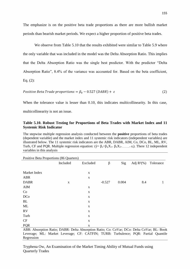
155
Tryphena Ow, An Examination of the Market Timing Ability of Mutual Funds using
Quarterly Trades
The emphasize is on the positive beta trade proportions as there are more bullish market
periods than bearish market periods. We expect a higher proportion of positive beta trades.
We observe from Table 5.10 that the results exhibited were similar to Table 5.9 where
the only variable that was included in the model was the Delta Absorption Ratio. This implies
that the Delta Absorption Ratio was the single best predictor. With the predictor “Delta
Absorption Ratio”, 8.4% of the variance was accounted for. Based on the beta coefficient,
Eq. (2):
𝑃𝑜𝑠𝑖𝑡𝑖𝑣𝑒 𝐵𝑒𝑡𝑎 𝑇𝑟𝑎𝑑𝑒 𝑝𝑟𝑜𝑝𝑜𝑟𝑡𝑖𝑜𝑛𝑠 = 𝛽0 − 0.527 (𝐷𝐴𝐵𝑅) + 𝜀 (2)
When the tolerance value is lesser than 0.10, this indicates multicollinearity. In this case,
multicollinearity is not an issue.
Table 5.10. Robust Testing for Proportions of Beta Trades with Market Index and 11
Systemic Risk Indicator
The stepwise multiple regression analysis conducted between the positive proportions of beta trades
(dependent variable) and the market index and 11 systemic risk indicators (independent variables) are
illustrated below. The 11 systemic risk indicators are the ABR, DABR, AIM, Co, DCo, BL, ML, RV,
Turb, CF and PQR. Multiple regression equation: (ŷ= βₒ+β₁X1+ β2X2+……….+ εi). There 12 independent
variables in this analysis
Positive Beta Proportions (86 Quarters)
Included Excluded β Sig Adj R²(%) Tolerance
Market Index
x
ABR
x
DABR x
-0.527 0.004 8.4 1
AIM
x
Co
x
DCo
x
BL
x
ML
x
RV
x
Turb
x
CF
x
PQR
x
ABR: Absorption Ratio; DABR: Delta Absorption Ratio; Co: CoVar; DCo: Delta CoVar; BL: Book
Leverage; ML: Market Leverage; CF: CATFIN; TURB: Turbulence; PQR: Partial Quantile
Regression
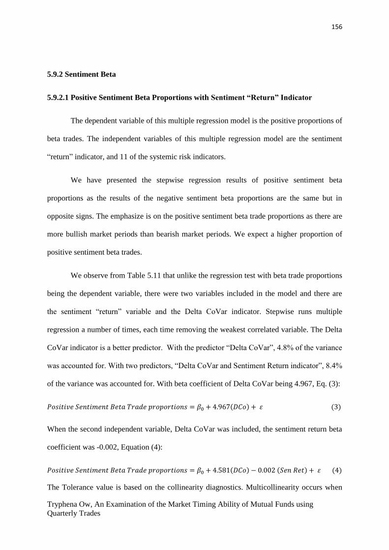
156
Tryphena Ow, An Examination of the Market Timing Ability of Mutual Funds using
Quarterly Trades
5.9.2 Sentiment Beta
5.9.2.1 Positive Sentiment Beta Proportions with Sentiment “Return” Indicator
The dependent variable of this multiple regression model is the positive proportions of
beta trades. The independent variables of this multiple regression model are the sentiment
“return” indicator, and 11 of the systemic risk indicators.
We have presented the stepwise regression results of positive sentiment beta
proportions as the results of the negative sentiment beta proportions are the same but in
opposite signs. The emphasize is on the positive sentiment beta trade proportions as there are
more bullish market periods than bearish market periods. We expect a higher proportion of
positive sentiment beta trades.
We observe from Table 5.11 that unlike the regression test with beta trade proportions
being the dependent variable, there were two variables included in the model and there are
the sentiment “return” variable and the Delta CoVar indicator. Stepwise runs multiple
regression a number of times, each time removing the weakest correlated variable. The Delta
CoVar indicator is a better predictor. With the predictor “Delta CoVar”, 4.8% of the variance
was accounted for. With two predictors, “Delta CoVar and Sentiment Return indicator”, 8.4%
of the variance was accounted for. With beta coefficient of Delta CoVar being 4.967, Eq. (3):
𝑃𝑜𝑠𝑖𝑡𝑖𝑣𝑒 𝑆𝑒𝑛𝑡𝑖𝑚𝑒𝑛𝑡 𝐵𝑒𝑡𝑎 𝑇𝑟𝑎𝑑𝑒 𝑝𝑟𝑜𝑝𝑜𝑟𝑡𝑖𝑜𝑛𝑠 = 𝛽0 + 4.967(𝐷𝐶𝑜) + 𝜀 (3)
When the second independent variable, Delta CoVar was included, the sentiment return beta
coefficient was -0.002, Equation (4):
𝑃𝑜𝑠𝑖𝑡𝑖𝑣𝑒 𝑆𝑒𝑛𝑡𝑖𝑚𝑒𝑛𝑡 𝐵𝑒𝑡𝑎 𝑇𝑟𝑎𝑑𝑒 𝑝𝑟𝑜𝑝𝑜𝑟𝑡𝑖𝑜𝑛𝑠 = 𝛽0 + 4.581(𝐷𝐶𝑜) − 0.002 (𝑆𝑒𝑛 𝑅𝑒𝑡) + 𝜀 (4)
The Tolerance value is based on the collinearity diagnostics. Multicollinearity occurs when
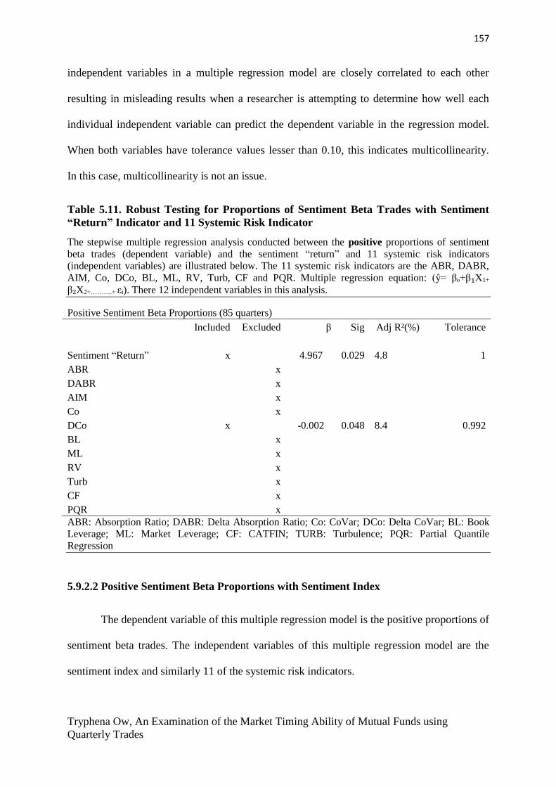
157
Tryphena Ow, An Examination of the Market Timing Ability of Mutual Funds using
Quarterly Trades
independent variables in a multiple regression model are closely correlated to each other
resulting in misleading results when a researcher is attempting to determine how well each
individual independent variable can predict the dependent variable in the regression model.
When both variables have tolerance values lesser than 0.10, this indicates multicollinearity.
In this case, multicollinearity is not an issue.
Table 5.11. Robust Testing for Proportions of Sentiment Beta Trades with Sentiment
“Return” Indicator and 11 Systemic Risk Indicator
The stepwise multiple regression analysis conducted between the positive proportions of sentiment
beta trades (dependent variable) and the sentiment “return” and 11 systemic risk indicators
(independent variables) are illustrated below. The 11 systemic risk indicators are the ABR, DABR,
AIM, Co, DCo, BL, ML, RV, Turb, CF and PQR. Multiple regression equation: (ŷ= βₒ+β₁X1+
β2X2+……….+ εi). There 12 independent variables in this analysis.
Positive Sentiment Beta Proportions (85 quarters)
Included Excluded β Sig Adj R²(%) Tolerance
Sentiment “Return” x
4.967 0.029 4.8 1
ABR
x
DABR
x
AIM
x
Co
x
DCo x
-0.002 0.048 8.4 0.992
BL
x
ML
x
RV
x
Turb
x
CF
x
PQR
x
ABR: Absorption Ratio; DABR: Delta Absorption Ratio; Co: CoVar; DCo: Delta CoVar; BL: Book
Leverage; ML: Market Leverage; CF: CATFIN; TURB: Turbulence; PQR: Partial Quantile
Regression
5.9.2.2 Positive Sentiment Beta Proportions with Sentiment Index
The dependent variable of this multiple regression model is the positive proportions of
sentiment beta trades. The independent variables of this multiple regression model are the
sentiment index and similarly 11 of the systemic risk indicators.

158
Tryphena Ow, An Examination of the Market Timing Ability of Mutual Funds using
Quarterly Trades
Similarly, we have presented the stepwise regression results of positive sentiment beta
proportions as the results of the negative sentiment beta proportions are the same but in
opposite signs. The emphasize is on the positive sentiment beta trade proportions as there are
more bullish market periods than bearish market periods. We expect a higher proportion of
positive sentiment beta trades.
We observe from Table 5.12 that unlike sentiment “return” indicator analysis in Table
5.11, the only variable that was included in the model was the Delta Absorption Ratio. This
implies that the Delta Absorption Ratio was the single best predictor for both beta and
sentiment trade proportions. With the predictor “Delta Absorption Ratio”, 8.4% of the
variance was accounted for. With -0.507 beta coefficient, Eq. (5):
𝑃𝑜𝑠𝑖𝑡𝑖𝑣𝑒 𝑆𝑒𝑛𝑡𝑖𝑚𝑒𝑛𝑡 𝑇𝑟𝑎𝑑𝑒 𝑝𝑟𝑜𝑝𝑜𝑟𝑡𝑖𝑜𝑛𝑠 = 𝛽0 − 0.507(𝐷𝐴𝐵𝑅) + 𝜀 (5)
When the tolerance value is lesser than 0.10, this indicates multicollinearity. In this case,
multicollinearity is not an issue.
Table 5.12. Robust Testing for Proportions of Sentiment Beta Trades with Sentiment
Index and 11 Systemic Risk Indicator
The stepwise multiple regression analysis conducted between the positive proportions of sentiment
beta trades (dependent variable) and the sentiment index and 11 systemic risk indicators (independent
variables) are illustrated below. The 11 systemic risk indicators are the ABR, DABR, AIM, Co, DCo,
BL, ML, RV, Turb, CF and PQR. Multiple regression equation: (ŷ= βₒ+β₁X1+ β2X2+……….+ εi). There
12 independent variables in this analysis
Positive Sentiment Beta Proportions (86 Quarters)
Included Excluded β Sig Adj R²(%) Tolerance
Sentiment Index
x
ABR
x
DABR x
-0.507 0.019 5.7 1
AIM
x
Co
x
DCo
x
BL
x
ML
x
RV
x
Turb
x

159
Tryphena Ow, An Examination of the Market Timing Ability of Mutual Funds using
Quarterly Trades
CF
x
PQR
x
ABR: Absorption Ratio; DABR: Delta Absorption Ratio; Co: CoVar; DCo: Delta CoVar; BL: Book
Leverage; ML: Market Leverage; CF: CATFIN; TURB: Turbulence; PQR: Partial Quantile
Regression
5.9.3 Momentum Trades
5.9.3.1 Positive Momentum Proportions with the Momentum “Return” Indicator
The dependent variable of this multiple regression model is the positive proportions of
momentum trades. The independent variables of this multiple regression model are the
momentum “return” indicator and similarly 11 of the systemic risk indicators.
We have presented the stepwise regression results of positive momentum proportions
as the results of the negative momentum proportions are the same but in opposite signs.
Although we observe from previous analysis that the number of quarters of negative
momentum trade proportions are higher, positive momentum trade proportions are presented
to stay consistent.
Based on Table 5.13, we observe that the only variable that was included in the model
was the CoVar indicator. This implies that the CoVar indicator was the single best predictor
for positive momentum trade proportions. With the predictor “CoVar”, 24.1 % of the
variance was accounted for. Based on the beta coefficient, Equation (6):
𝑃𝑜𝑠𝑖𝑡𝑖𝑣𝑒 𝑀𝑜𝑚𝑒𝑛𝑡𝑢𝑚 𝑇𝑟𝑎𝑑𝑒 𝑝𝑟𝑜𝑝𝑜𝑟𝑡𝑖𝑜𝑛𝑠 = 𝛽0 − 4.294(𝐶𝑜) + 𝜀 (6)
When the tolerance value is lesser than 0.10, this indicates multicollinearity. In this case,
multicollinearity is not an issue.
Table 5.13. Robust Testing for Proportions of Momentum Trades with Momentum
“Return” Indicator and 11 Systemic Risk Indicator
The stepwise multiple regression analysis conducted between the positive proportions of momentum
trades (dependent variable) and the momentum “return” indicator and 11 systemic risk indicators

160
Tryphena Ow, An Examination of the Market Timing Ability of Mutual Funds using
Quarterly Trades
(independent variables) are illustrated below. The 11 systemic risk indicators are the ABR, DABR,
AIM, Co, DCo, BL, ML, RV, Turb, CF and PQR. Multiple regression equation: (ŷ= βₒ+β₁X1+
β2X2+……….+ εi). There 12 independent variables in this analysis
Positive Momentum Proportions (24 Quarters)
Included Excluded β Sig Adj R²(%) Tolerance
Momentum “Return”
x
ABR
x
DABR
x
AIM
x
Co x
-4.294 0.009 24.1 1
DCo
x
BL
x
ML
x
RV
x
Turb
x
CF
x
PQR
x
ABR: Absorption Ratio; DABR: Delta Absorption Ratio; Co: CoVar; DCo: Delta CoVar; BL: Book
Leverage; ML: Market Leverage; CF: CATFIN; TURB: Turbulence; PQR: Partial Quantile
Regression
5.9.3.2 Positive Momentum Proportions with Momentum Index
The dependent variable of this multiple regression model is the positive proportions of
momentum trades. The independent variables of this multiple regression model are the
momentum index and similarly 11 of the systemic risk indicators.
Similarly, we have presented the stepwise regression results of positive momentum
proportions as the results of the negative momentum proportions are the same but in opposite
signs. Although we observe from previous analysis that the number of quarters of negative
momentum trade proportions are higher, positive momentum trade proportions are reflected
to keep consistency in presentation.
We observe from Table 5.14, we observe that similar to the momentum “return”
indicator, the only variable that was included in the model was the CoVar indicator. This
161
Tryphena Ow, An Examination of the Market Timing Ability of Mutual Funds using
Quarterly Trades
implies that the CoVar indicator was the single best predictor for negative momentum trade
proportions. With the predictor “CoVar”, 24.8 % of the variance was accounted for. Based on
the beta coefficient, Equation (7):
𝑃𝑜𝑠𝑖𝑡𝑖𝑣𝑒 𝑀𝑜𝑚𝑒𝑛𝑡𝑢𝑚 𝑇𝑟𝑎𝑑𝑒 𝑝𝑟𝑜𝑝𝑜𝑟𝑡𝑖𝑜𝑛𝑠 = 𝛽0 − 4.252(𝐶𝑜) + 𝜀 (7)
When the tolerance value is lesser than 0.10, this indicates multicollinearity. In this case,
multicollinearity is not an issue.
Table 5.14. Robust Testing for Proportions of Momentum Trades with Momentum
Index and 11 Systemic Risk Indicator
The stepwise multiple regression analysis conducted between the positive proportions of momentum
trades (dependent variable) and the momentum index and 11 systemic risk indicators (independent
variables) are illustrated below. The 11 systemic risk indicators are the ABR, DABR, AIM, Co, DCo,
BL, ML, RV, Turb, CF and PQR. Multiple regression equation: (ŷ= βₒ+β₁X1+ β2X2+……….+ εi). There
12 independent variables in this analysis
Negative Momentum Proportions (25 Quarters)
Included Excluded β Sig Adj R²(%) Tolerance
Momentum Index
x
ABR
x
DABR
x
AIM
x
Co x
-4.252 0.007 24.8 1
DCo
x
BL
x
ML
x
RV
x
Turb
x
CF
x
PQR
x
ABR: Absorption Ratio; DABR: Delta Absorption Ratio; Co: CoVar; DCo: Delta CoVar; BL: Book
Leverage; ML: Market Leverage; CF: CATFIN; TURB: Turbulence; PQR: Partial Quantile
Regression
162
Tryphena Ow, An Examination of the Market Timing Ability of Mutual Funds using
Quarterly Trades
5.10 Summary Table of Significant Results based on Robust and Multiple Regression
Tests
Table 5.15. Significant Results based on Robust and Multiple Regression tests
The table below summarises the significant results of the robust and multiple regression test. Panel A
presents the significant results of the robust test. Panel B represents the significant results of the
multiple regression test. √ represents significant results, × represents no significant results exhibited.

163
Tryphena Ow, An Examination of the Market Timing Ability of Mutual Funds using
Quarterly Trades
5.11 Conclusion of Robust Testing
This chapter focus on market timing abilities of mutual fund managers through
various robust tests. Robust tests are conducted between the statistically significant trade
proportions that encompass beta, sentiment beta and momentum and their respective market
Panel A: Robust Test
Types of Test Types of
Trades
Positive Negative Types of
Indicators
Correlation Regression
Changes in Signs Beta √ Market "Ret" × √
Sentiment Beta √ Sentiment "Ret" √ √
Persistence Beta √ Market "Ret" × √
Beta √ Market Index × √
Sentiment Beta √ Sentiment "Ret" √ √
Momentum √ Momentum "Ret" × √
Momentum √ Momentum Index √ √
Panel B: Multiple Regression
Types of Trade
(DV)
Types of
Indicators (IV)
No. of
Excluded Var
No. of Included
Var
Included
Var(s)
Adjusted
R²(%)
Beta Market "Ret" 11 Systemic Risk 11 1 DABR 8.1
Market Index 11 Systemic Risk 11 1 DABR 8.4
Sentiment Beta Sentiment "Ret" 11 Systemic Risk 10 2 Sen "Ret"; Dco 4.8; 8.4
Sentiment Index 11 Systemic Risk 11 1 DABR 5.7
Momentum Momentum "Ret" 11 Systemic Risk 11 1 Co 24.1
Momentum Index 11 Systemic Risk 11 1 Co 24.8
Var: Variables; DV: Dependent Var; IV: Independent Var; DABR: Delta Absorption Ratio; Dco: Delta CoVar; Co: CoVar

164
Tryphena Ow, An Examination of the Market Timing Ability of Mutual Funds using
Quarterly Trades
indicators. The adjustments of positive and negative trade proportions are dependent on the
forecast of the market. In the previous chapter, we examine the abilities of fund managers to
isolate turning points in the market’s economic and financial behaviour. Our results showed
that the sentiment and momentum trade proportions exhibited an inverse relationship with
their respective indicators. We investigate further on the significant relationship between
these variables by conducting various robust tests.
We consider several conditions that might influence the changes in the values of these
market indicators. These indicators reflect the performance of the market henceforth fund
managers can take advantage of the market by adjusting their portfolio accordingly. There are
four types of robust test, magnitude of changes, changes in standard deviation, change in
signs and market persistence.
The “magnitude of change” and the “changes in standard deviation” tests focus on the
“returns” of the market index. These test are conducted between the beta trade proportions
and the market “return” indicator. The “magnitude of change” test attempts to identify fund
managers that are capable of selecting big or small changes based on the market “returns”.
This test is conducted between the beta trade proportions and the market “return” indicator.
Similarly, the “changes in standard deviation” test attempts to identify fund managers that are
capable of selecting changes based on returns that 38% (half a standard deviation) above the
mean or 38% (half a standard deviation) below the mean. This test identifies how confident a
fund manager is at selecting changes. However, our results did not exhibit any significant
results between the beta trade proportions and the market “return” indicator.
The “changes in signs” test focus on the ability of mutual funds to select turning
points of the index based on the values of the indicators. When the values of the indicators
transit from positive (negative) to negative (positive) values, this could be a signal that

165
Tryphena Ow, An Examination of the Market Timing Ability of Mutual Funds using
Quarterly Trades
market conditions are changing suggesting an upcoming bear (bull) market. We expect
mutual fund managers to adjust their portfolios towards negative (positive) trade proportions.
However, this test can only be conducted on indicators that are free from spurious issues.
We conducted the “changes in signs” test between these trade proportions and their
respective indicators: beta trade proportions and the market “return” indicator; the sentiment
beta trade proportions and the sentiment “return” indicator; the sentiment beta trade
proportions and the sentiment index. The only significant correlation and regression results
was exhibited between the positive sentiment beta trade proportions and the sentiment
“return” indicator. Results suggest an inverse relationship between these variables.
The “persistence” test identifies fund managers that adjust their portfolios according
to the persistence in index values. We examine how “persistence” of the values of the market
indicators and their respective trade proportions. Significant correlation and regression results
were present between the positive sentiment trade proportions and the sentiment “return”
indicator. Similar to the “changes in signs” test, results suggest an inverse relationship.
Significant correlation and regression results were also present between the positive
momentum trade proportions and the momentum index. Consistent to our findings, results
also suggest an inverse relationship.
Similar to previous findings, it is plausible based on the results of the correlation and
regression analysis that fund managers might have undertaken a contrarian strategy as most
correlation results reflected an inverse relationship between the trade proportions and the
market indicators. As these results were not consistent to our expectations, we investigate
further by conducting a multiple regression analysis.
Previously, simple regression analyses were conducted, concentrating on how one
independent variable (market indicators, “return” indicators and systemic risk indicators)

166
Tryphena Ow, An Examination of the Market Timing Ability of Mutual Funds using
Quarterly Trades
might affect the dependent variable (trade proportions). By conducting a multiple regression
analysis, we consider how two or more independent variables, be it market or systemic risk
indicators might simultaneously affect the predictability value of the statistically significant
trade proportions. Although there were some significant regression results, the multiple
regression test did not reflect any new evidence on the existence of market timing abilities of
these statistically significant trade proportions.
Overall, based on these results, there were insufficient evidence to substantiate that
fund managers possess market timing abilities based on examination of their statistically
significant trade proportions. However, consistent results were displayed from the analyses
between the sentiment trade proportions, the momentum trade proportions and their
respective indicators. Both sentiment and momentum trade proportions exhibited an inverse
relationship with their respective indicators. Furthermore, contrary to our expectations,
despite momentum trade proportions having the least number of quarter observations, these
trade proportions produced the most number of significant results. Interestingly, we did not
find any significant results from the beta trade proportions. In the next chapter, we conclude
the findings, discuss the limitations of this study and also discuss suggestions for future
research.
CHAPTER 6
CONCLUSION
6.1 Introduction

167
Tryphena Ow, An Examination of the Market Timing Ability of Mutual Funds using
Quarterly Trades
This chapter concludes our thesis. In this chapter, we provide an overview of our
study, identify the limitations and offer suggestions for future research.
6.2 Overview of Conclusion
The performance measures for market timing abilities of mutual fund managers have
been evolving over the years. In our study, we define market timing as the ability of fund
managers to adjust their portfolios in accordance to the anticipated market trends to take
advantage of the market. Common market trends are the bull, bear, recession and boom
periods.
Majority of the performance measures studied the returns and stockholdings of mutual
funds but on average, found no significant market timing abilities. Using a different
approach, Chen, Jegadeesh and Wermers (2000) evaluated market timing abilities using
mutual funds trades and argued that active stock trades represent a stronger opinion of a
manager as compared to “passive” stock holdings.
Similar to the study of Chen et al. (2000), we evaluated the market timing abilities of
fund managers using mutual fund trades. We obtained the statistically significant trade betas
of US equity mutual funds from the data provided by Cullen et al. (2015). There were 62,676
fund quarters and 86 quarters. These statistically significant trades encompass beta, sentiment
beta and momentum. Using a new approach, we evaluated these trades using proportions as
they provide some insights on the direction that the fund manager is pursuing in each quarter.
When the market is anticipated to be bullish or in expansion, we expect a higher proportion
of positive trades. When the market is anticipated to be bearish or undergoing a recession
period, we expect a higher proportion of negative trades. The act of adjusting between
positive and negative trade proportions in accordance to bullish and bearish markets is similar
to the study by Jiang, Yao and Yu (2007) which stated that a fund manager with market
168
Tryphena Ow, An Examination of the Market Timing Ability of Mutual Funds using
Quarterly Trades
timing abilities would increase and decrease beta exposure according to macroeconomic
variables. Although risk shifting can be done when a skilled fun manager takes advantage of
their market timing abilities, Huang, Sialm and Zhang (2011) explained that risk shifting
could also be a signal of ill motivated trades either from inferior ability of fund managers or
agency issues.
Previously, Avamov and Wermers (2006) found that predictability skills are best
performed during recession periods but also present in expansion periods. Likewise for our
study, we have considered both “up” and “down” market trends. Our period of study was
between 1991 and 2012. There were three bull market periods and two bear market periods.
There were also three expansion periods and two recession periods. There were similar
numbers of “up” market trends and “down” market trends as bear market periods are highly
associated to recession periods. Therefore, our trade proportions were tested during volatile
conditions.
Market and systemic risk indicators are important for our study as they reflect the
performance of the market. Market indicators signal periods of upcoming bullish and bearish
markets. Systemic risk indicators reflect the performance of the economy. After the recession
global financial crisis, systemic risk indicators were created to signal upcoming recession
periods. We considered how bullish and bearish market periods will influence the
adjustments of positive or negative trade proportions. We also conducted various robust tests
that identify if fund managers were capable of picking small or big changes, how confident
they are at picking changes, picking turning points of the market and how market persistence
affects their trading decisions. We conducted a series of correlation and regression tests
between these statistically significant trade proportions (dependent variable) and their
respective market and systemic risk indicators (independent variables). We observed if these
variables co vary and if so exhibit a direct or inverse relationship.

169
Tryphena Ow, An Examination of the Market Timing Ability of Mutual Funds using
Quarterly Trades
6.3 Significant Research Findings
We observed from the results of the correlation and regression analysis, momentum
trade proportions displayed the most number of significant results despite having the least
number of quarters. However, results were inconsistent to our expectations that during bullish
periods, fund managers will adjust their portfolios towards positive trade proportions. Instead,
results suggest that these fund managers have adjusted their portfolios towards negative trade
proportions during bullish market periods. It is likely that these mutual fund managers were
pursuing a contrarian strategy. Lo and Mackinaly (1990) discussed that contrarian strategies
are strategies that go against market trends by purchasing assets that were past “losers” and
selling assets that were past “winners”. Cullen, Gasbarro, Zumwalt and Monroe (2009)
examined the trading activities of mutual funds to determine if they had adjusted their
portfolios towards stocks that were recent “winners” (momentum strategy) or recent “losers”
(contrarian strategy). They reported that a contrarian strategy is said to be profitable when the
market overreacts as fund managers that followed a momentum strategy will cause the prices
of “winners” to rapidly increase and eventually these “winners” will become losers.
It is plausible that market timing abilities were exhibited from these statistically
significant trade proportions when fund managers pursued a contrarian strategy. Our results
also suggest long term persistence in the market timing abilities of mutual funds. Previously,
Bollen and Busse (2005) studied the daily returns of 230 mutual funds between 1985 and
1995 and concluded that market timing abilities were only significant when evaluated in a
short term period but cease to exist when funds are evaluated over a longer time horizon.
6.4 Limitations of the Research
Our study focused on evaluating the market timing abilities of fund managers using
quarterly observations of the statistically significant trade proportions. Using quarterly data

170
Tryphena Ow, An Examination of the Market Timing Ability of Mutual Funds using
Quarterly Trades
observations give fund managers more time allowance to form market expectations and
adjust their portfolios accordingly. However, it also imposed some limitations on this study.
As mutual fund managers may have higher trading frequencies, quarterly data observations
may not be able to capture sufficient information. We considered how daily, monthly or
weekly data will reflect the frequent trading activities of mutual funds.
We considered how the number of quarters might affect the results of our analysis. In
this study, there were 86 quarters available for our analysis. Although momentum trade
proportions displayed significant results with only 25 quarters, it is plausible that the
correlation and regression results between the beta and sentiment beta trade proportions and
their respective indicators were affected by the number of quarters. Furthermore, we observed
from the robust tests that there were less than 30 observations of quarters.
It is also possible that the use of only statistically significant trade proportions have
affected the results of our study. In this case, we used 5% significance level to select trades in
a specific direction. It would be useful to examine whether different significance levels result
in different findings. However, the use of ratios of may mitigate any differences.
We also considered if the use of trade proportions have biased our analysis process as
proportions are affected by the level of statistical significance. The lower the significance
level is, the more number of trades which will impact the proportions of positive and negative
trades. Proportions might be also be disadvantage due to a small denominator arising when
we increase the statistical significance.
6.5 Areas of Future Research
Former studies focused on evaluating market timing abilities in recession periods
only. On the other hand, similar to Avamov and Wemers (2006), we have considered both
recession and expansion periods in our analysis. During the study of Avamov and Wemers

171
Tryphena Ow, An Examination of the Market Timing Ability of Mutual Funds using
Quarterly Trades
(2006) which was between 1975 and 2002, there were two recession periods. Similarly
between 1991 and 2012, there were also two recession periods. We considered how future
research may examine market timing abilities based on a longer time period which includes
all four recession periods and expansion periods.
Future research might also consider evaluating the market timing abilities of trade
proportions based on daily, weekly or monthly data observations to capture higher trading
frequencies of trading activities. Elton, Gruber and Blake (2012) reported that 18.5% of
trades by an average fund manager were not detected when market timing measures were
applied to quarterly data holdings. Additionally, this study was based on 5% statistically
significant trade proportions, future research might consider using 1% or 10% statistical
significance as the proportion analysis may reveal different results. For example, using 10%
(1%) significance level will increase (decrease) the number of significant trades.
Majority of the research evaluated market timing abilities of mutual fund managers
without considering the existence of stock selection abilities. Unlike majority of the research,
Chang and Lewellen (1984) believed that fund managers might exploit returns by engaging in
effective “macro” market timing activities along with cautious “micro” stock selection
efforts. They examined the monthly returns of 67 mutual funds and evaluated market timing
abilities of mutual funds while simultaneously evaluating stock selection abilities in mutual
funds. However, there were no evidence of market timing abilities. An additional study by
Chen and Stockum (1986) also investigated mutual fund’s selectivity and timing skills
simultaneously using the quarterly returns of 43 funds. Although stock selection ability was
present, there were still no market timing skills exhibited.
Using a different approach the study by Kacperczyk, Nieuwerburgh and Veldkamp
(2014) found market timing abilities while simultaneously investigating the stock selection

172
Tryphena Ow, An Examination of the Market Timing Ability of Mutual Funds using
Quarterly Trades
abilities of mutual fund managers using equity mutual fund holdings. Their methodology
focused on skills of managers by giving more weightage of a fund’s market timing more in
recession periods and stock picking in booms. Future research may examine the trade
proportions of mutual funds instead of fund holdings, similarly by giving more weightage of
a fund’s market timing more in recession periods and stock picking in booms. Giving
considerations that the skills of fund managers might alter accordingly to different business
cycles.
We have also considered the study by Jiang and Fang (2015) that suggested two other
states in the business cycles besides the bull and bear markets. Based on the volatility factor
in stock returns, business cycles have been broken down into the “extreme bear market”, “the
general bear market”, “the volatile bull market” and the “steady bull market”. However, we
were unable to pursue this area of research as there were insufficient data to permit this
partitioning. Future research might consider incorporating all four states of the business cycle
in their studies.
6.6 Summary of Study
Using a new approach, our study focused on evaluating market timing abilities using
trade proportions. Trade proportions give us some insights on the direction that the fund
manager was pursuing. Our trading period between the year 1991 and 2012 had three bullish
markets and two bearish markets. We developed a method that studies how the values of the
market and systemic risk indicators which reflect different market trends might influence a
fund manager to adjust his or her portfolios. Using correlation and regression analysis, we
examined the relationships between these variables.
We found the most significant results between momentum trade proportions and the
momentum indicators. It is probable that these fund managers have undertaken a contrarian
173
Tryphena Ow, An Examination of the Market Timing Ability of Mutual Funds using
Quarterly Trades
strategy as their positive momentum trade proportions had an inverse relationship with the
momentum index during bullish market periods. However, results were only significant from
the momentum trade proportions. Therefore, we are unable to conclude that fund managers
possess market timing abilities. Further research employing our approach with a longer
examination period, with an associated increase in observations, will provide supplementary
evidence on market timing abilities.
REFERENCES
Acharya, V. V., Pedersen, L. H., Philippon, T., & Richardson, M. P. (2010).
Measuring systemic risk. Unpublished Working Paper. New York University
Adrian, T., & Brunnermeier, M. K. (2011). CoVaR (No. w17454). National Bureau of
Economic Research.

174
Tryphena Ow, An Examination of the Market Timing Ability of Mutual Funds using
Quarterly Trades
Allen, L., Bali, T. G., & Tang, Y. (2012). Does systemic risk in the financial sector
predict future economic downturns?. Review of Financial Studies, 25(10), 3000-3036.
Amadeo, K. (2016). The History of Recessions in the United States. Retrieved from:
https://www.thebalance.com/what-is-a-recession-3306019
Amihud, Y. (2002). Illiquidity and stock returns: cross-section and time-series effects.
Journal of Financial Markets, 5(1), 31-56.
Avramov, D., & Wermers, R. (2006). Investing in mutual funds when returns are
predictable. Journal of Financial Economics, 81(2), 339-377.
Baker, M., & Wurgler, J. (2007). Investor sentiment in the stock market. The Journal
of Economic Perspectives, 21(2), 129-151.
Baker, M., Litov, L., Wachter, J. A., & Wurgler, J. (2010). Can mutual fund managers
pick stocks? Evidence from their trades prior to earnings announcements. Journal of
Financial and Quantitative Analysis, 45(5), 1111.
Barnes, R. (2016). The Fuel That Fed The Subprime Meltdown. Retrieved from:
http://www.investopedia.com/articles/07/subprime-
overview.asp?ad=dirN&qo=investopediaSiteSearch&qsrc=0&o=40186
Beattie, A. (2016). Market Crashes: The Dotcom Crash. Retrieved from:
http://www.investopedia.com/features/crashes/crashes8.asp?ad=dirN&qo=investopediaSiteSe
arch&qsrc=0&o=40186
Billio, M., Getmansky, M., Lo, A. W., & Pelizzon, L. (2012). Econometric measures
of connectedness and systemic risk in the finance and insurance sectors. Journal of Financial
Economics, 104(3), 535-559.

175
Tryphena Ow, An Examination of the Market Timing Ability of Mutual Funds using
Quarterly Trades
Black, K., Asafu-Adjaye, J., Burke, P., Khan, N., King, G., Perera, N., Papadimos A.,
Sherwood C., Wasimi S & Verma R. (2016). Australasian Business Statistics. John Wiley
and Sons, Ltd.
Bollen, N. P., & Busse, J. A. (2005). Short-term persistence in mutual fund
performance. Review of Financial Studies, 18(2), 569-597.
Bormann, S. K. (2013). Sentiment indices on financial markets: What do they
measure?. Kiel Institute for the World Economy, Economics Discussion Paper, 58, 2013.
Brownlees, C. T., Engle, R. F., & Kelly, B. T. (2011). A practical guide to volatility
forecasting through calm and storm. Journal of Risk, 14(2), 1-22.
Busse, J. A. (1999). Volatility timing in mutual funds: Evidence from daily returns.
Review of Financial Studies, 12(5), 1009-1041.
Chang, E. C., & Lewellen, W. G. (1984). Market timing and mutual fund investment
performance. Journal of Business, 57-72.
Chen, C. R., & Stockum, S. (1986). Selectivity, market timing, and random beta
behavior of mutual funds: A generalized model. Journal of Financial Research, 9(1), 87-96.
Chen, S. N. (1982). An examination of risk-return relationship in bull and bear
markets using time-varying betas. Journal of Financial and Quantitative Analysis, 17(02),
265-286.
Chen, H. L., Jegadeesh, N., & Wermers, R. (2000). The value of active mutual fund
management: An examination of the stockholdings and trades of fund managers. Journal of
Financial and Quantitative Analysis, 35(03), 343-368.
Chen, S. S., Chou, Y. H., & Yen, C. Y. (2016). Predicting US recessions with stock
market illiquidity. The BE Journal of Macroeconomics, 16(1), 93-123.

176
Tryphena Ow, An Examination of the Market Timing Ability of Mutual Funds using
Quarterly Trades
Chen, Y. T., & Vincent, K. (2016). The Role of Momentum, Sentiment, and
Economic Fundamentals in Forecasting Bear Stock Market. Journal of Forecasting, 35(6),
504-527
Cohen, J. B., Zinbarg, E. D., & Zeikel, A. (1973). Investment Analysis and Portfolio
Management (Revised Edition ed.): RD Irwin Co.
Cullen, G., Gasbarro, D., Monroe, G. S., & Zumwalt, J. K. (2009). Systematic Risk
and the Performance of Mutual Funds Pursuing Momentum and Contrarian Trades. In 22nd
Australasian Finance and Banking Conference.
Cullen, G., Gasbarro, D., Monroe, G. S., & Zumwalt, J. K. (2010t). Investor sentiment
and the performance of mutual funds pursuing momentum and contrarian trading strategies.
In 23rd Australasian Finance and Banking Conference.
Dan, B. (2014). A Review of Past Recessions. Retrieved from:
http://www.investopedia.com/articles/economics/08/past-recessions.asp
Davis, M. (2011). How September 11 Affected The U.S. Stock Market. Retrieved
from: http://www.investopedia.com/financial-edge/0911/how-september-11-affected-the-u.s.-
stock-market.aspx
Diebold, F. X., & Yilmaz, K. (2009). Measuring financial asset return and volatility
spillovers, with application to global equity markets. The Economic Journal, 119(534), 158-
171.
Elton, E. J., Gruber, M. J., & Blake, C. R. (2012). An examination of mutual fund
timing ability using monthly holdings data. Review of Finance, 16(3), 619-645.
Fabozzi, F. J., & Francis, J. C. (1979). Mutual fund systematic risk for bull and bear
markets: an empirical examination. The Journal of Finance, 34(5), 1243-1250.

177
Tryphena Ow, An Examination of the Market Timing Ability of Mutual Funds using
Quarterly Trades
Ferri, M. G., Oberhelman, H. D., & Roenfeldt, R. L. (1984). Market timing and
mutual fund portfolio composition. Journal of Financial Research, 7(2), 143-150.
Giglio, S., Kelly, B., & Pruitt, S. (2016). Systemic risk and the macroeconomy: An
empirical evaluation. Journal of Financial Economics, 119(3), 457-471.
Gilchrist, S., & Zakrajšek, E. (2012). Credit spreads and business cycle fluctuations.
The American Economic Review, 102(4), 1692-1720.
Grinblatt, M., & Titman, S. (1989). Mutual fund performance: An analysis of
quarterly portfolio holdings. Journal of Business, 393-416.
Grinblatt, M., & Titman, S. (1993). Performance measurement without benchmarks:
An examination of mutual fund returns. Journal of Business, 47-68.
Henrikson, R., & Merton, R. (1981). On market timing and investment
performance. Journal of Finance, 33, 1051-1099.
Huang, J., Sialm, C., & Zhang, H. (2011). Risk shifting and mutual fund performance.
Review of Financial Studies, 24(8), 2575-2616.
Investopedia (2016). Standard & Poor's 500 Index - S&P 500. Retrieved from
http://www.investopedia.com/terms/s/sp500.asp
Investopedia (2016). Chicago Board Options Exchange – CBOE. Retrieved from
http://www.investopedia.com/terms/c/cboe.asp
Investopedia (2016). Industrial Production Index – IPI. Retrieved from
http://www.investopedia.com/terms/i/ipi.asp
Investopedia (2016). VIX - CBOE Volatility Index. Retrieved from
http://www.investopedia.com/terms/v/vix.asp
178
Tryphena Ow, An Examination of the Market Timing Ability of Mutual Funds using
Quarterly Trades
Jensen, M. C. (1968). The performance of mutual funds in the period 1945–1964. The
Journal of Finance, 23(2), 389-416.
Jiang, Y., & Fang, X. (2015). Bull, bear or any other states in US stock market?.
Economic Modelling, 44, 54-58.
Jiang, G. J., Yao, T., & Yu, T. (2007). Do mutual funds time the market? Evidence
from portfolio holdings. Journal of Financial Economics, 86(3), 724-758.
Johnsson, E., & Karlsson, J. (2016). Performance of hedge fund strategies in bull and
bear markets. (Bachelor Thesis). University of Gothenburg.
Kacperczyk, M., NIEUWERBURGH, S. V., & Veldkamp, L. (2014). Time‐Varying
Fund Manager Skill. The Journal of Finance, 69(4), 1455-1484.
Karceski, J. (2002). Returns-chasing behavior, mutual funds, and beta's death. Journal
of Financial and Quantitative analysis, 37(04), 559-594.
Kim, M. K., & Zumwalt, J. K. (1979). An analysis of risk in bull and bear markets.
Journal of Financial and Quantitative analysis, 14(05), 1015-1025.
Kritzman, M., Li, Y., Page, S., & Rigobon, R. (2010). Principal components as a
measure of systemic risk. Working Paper, Revere Street.
Lo, A. W., & MacKinlay, A. C. (1990). When are contrarian profits due to stock
market overreaction?. Review of Financial Studies, 3(2), 175-205.
Logan, T. (2014). Profiting from Market Trends: Simple Tools and Techniques for
Mastering Trend Analysis. John Wiley & Sons.
Menkhoff*, L., & Schmidt, U. (2005). The use of trading strategies by fund
managers: some first survey evidence. Applied Economics, 37(15), 1719-1730.
179
Tryphena Ow, An Examination of the Market Timing Ability of Mutual Funds using
Quarterly Trades
Miller, T. W., & Gressis, N. (1980). Nonstationarity and evaluation of mutual fund
performance. Journal of Financial and Quantitative Analysis, 15(03), 639-654.
Mitchell, C. (2016). Can Perpetual Contrarians Profit As Traders. Retrieved from:
http://www.investopedia.com/articles/trading/10/profit-as-a-perpetual-contrarian.asp
Moskowitz, T. J. (2000). Discussion. The Journal of Finance, 55(4), 1695-1703.
Pinnuck, M. (2003). An examination of the performance of the trades and stock
holdings of fund managers: Further evidence. Journal of Financial and Quantitative
Analysis, 38(04), 811-828.
Prather, L. J., Middleton, K. L., & Cusack, A. J. (2001). Are N+ 1 heads better than
one? The timing and selectivity of Australian-managed investment funds. Pacific-Basin
Finance Journal, 9(4), 379-400.
Russell, R. (2007). An introduction to mutual funds worldwide. John Wiley & Sons.
Standard & Poor’s. (2016). S&P Dow Jones Indices: Index Methodology. Retrieved
from: https://us.spindices.com/documents/methodologies/methodology-sp-us-indices.pdf
Standard & Poor’s. (2016). S&P Dow Jones Indices: Contrarian Opportunities Index
Methodology. Retrieved from:
https://www.djindexes.com/mdsidx/downloads/meth_info/Dow_Jones_US_Contrarian_Oppo
rtunities_Index_Methodology.pdf
Standard & Poor’s. (2016). S&P Dow Jones Indices: Quality Indices Methodology.
Retrieved from: http://www.spindices.com/documents/methodologies/methodology-sp-
quality-indices.pdf

180
Tryphena Ow, An Examination of the Market Timing Ability of Mutual Funds using
Quarterly Trades
Standard & Poor’s. (2016). S&P Dow Jones Indices: Low Volatility Index
Methodology. Retrieved from:
http://us.spindices.com/documents/methodologies/methodology-sp-low-volatility-indices.pdf
Standard & Poor’s. (2016). S&P Dow Jones Indices: Growth Index Methodology.
Retrieved from: http://au.spindices.com/indices/equity/sp-500-growth
Standard & Poor’s. (2016). S&P Dow Jones Indices: Dividend Points Index
Methodology. Retrieved from: https://au.spindices.com/indices/equity/sp-500-dividend-
points-index-annual
StockCharts (2016). Volatility Index (VIX). Retrieved from
http://stockcharts.com/school/doku.php?id=chart_school:technical_indicators:volatility_inde
x
The National Bureau of Economic Research. (2016). US Business Cycles Expansions
and Contractions. Retrieved from: http://www.nber.org/cycles.html
Treynor, J., & Mazuy, K. (1966). Can mutual funds outguess the market. Harvard
business review, 44(4), 131-136.
Wermers, R. (2000). Mutual fund performance: An empirical decomposition into
stock‐picking talent, style, transactions costs, and expenses. The Journal of Finance, 55(4),
1655-1703.
Williamson, J. P. (1972). Measurement and forecasting of mutual fund performance:
choosing an investment strategy. Financial Analysts Journal, 28(6), 78-84.


![The Salvation Army NZ, Fiji, Tonga & Samoa Women’s Ministriesfile_field:type]/a6_wm... · Claudia Procula Joanna Tryphena Tryphosa Persis Mary Lydia lois Phoebe Priscilla Eunice](https://img.pdfslide.net/doc/110x75/5e031d2cd9e2ea2f2041d260/the-salvation-army-nz-fiji-tonga-samoa-womenas-ministries-filefieldtypea6wm.jpg)