TutorialandManualforGeostatisticalAnalyseswith … theRpackagegeorob ... and A is a matrix that is used to model geometrically ... (Hofer and Papritz,

Tutorial and Manual for Geostatistical Analyses with

the R package georob

Andreas Papritz

January 26, 2018

Contents

1 Summary 3

2 Introduction 32.1 Model . . . . . . . . . . . . . . . . . . . . . . . . . . . . . . . . . . . . . . 32.2 Estimation . . . . . . . . . . . . . . . . . . . . . . . . . . . . . . . . . . . . 42.3 Prediction . . . . . . . . . . . . . . . . . . . . . . . . . . . . . . . . . . . . 52.4 Functionality . . . . . . . . . . . . . . . . . . . . . . . . . . . . . . . . . . 5

3 Model-based Gaussian analysis of zinc, data set meuse 73.1 Exploratory analysis . . . . . . . . . . . . . . . . . . . . . . . . . . . . . . 73.2 Fitting a spatial linear model by Gaussian (RE)ML . . . . . . . . . . . . . 133.3 Computing Kriging predictions . . . . . . . . . . . . . . . . . . . . . . . . 20

3.3.1 Lognormal point Kriging . . . . . . . . . . . . . . . . . . . . . . . . 203.3.2 Lognormal block Kriging . . . . . . . . . . . . . . . . . . . . . . . . 22

4 Robust analysis of coalash data 264.1 Exploratory analysis . . . . . . . . . . . . . . . . . . . . . . . . . . . . . . 264.2 Fitting a spatial linear model robust REML . . . . . . . . . . . . . . . . . 324.3 Computing robust Kriging predictions . . . . . . . . . . . . . . . . . . . . 43

4.3.1 Point Kriging . . . . . . . . . . . . . . . . . . . . . . . . . . . . . . 434.3.2 Block Kriging . . . . . . . . . . . . . . . . . . . . . . . . . . . . . . 45

5 Details about parameter estimation 495.1 Implemented variogram models . . . . . . . . . . . . . . . . . . . . . . . . 495.2 Estimating parameters of power function variogram . . . . . . . . . . . . . 495.3 Estimating parameters of geometrically anisotropic variograms . . . . . . . 495.4 Estimating variance of micro-scale variation . . . . . . . . . . . . . . . . . 505.5 Estimating variance parameters by Gaussian (RE)ML . . . . . . . . . . . . 505.6 Constraining estimates of variogram parameters . . . . . . . . . . . . . . . 515.7 Computing robust initial estimates of parameters for robust REML . . . . 515.8 Estimating parameters of “nested” variogram models . . . . . . . . . . . . 525.9 Controlling georob() by the function control.georob() . . . . . . . . . . 52

5.9.1 Gaussian (RE)ML estimation . . . . . . . . . . . . . . . . . . . . . 525.9.2 Robust REML estimation . . . . . . . . . . . . . . . . . . . . . . . 53

1

5.9.3 Approximation of covariances of fixed and random effects and residuals 535.9.4 Transformations of variogram parameters for (RE)ML estimation . 545.9.5 Miscellaneous arguments of control.georob() . . . . . . . . . . . 54

5.10 Parallelized computations . . . . . . . . . . . . . . . . . . . . . . . . . . . 55

6 Details about Kriging 576.1 Functionality of predict.georob() . . . . . . . . . . . . . . . . . . . . . . 57

6.1.1 Prediction targets . . . . . . . . . . . . . . . . . . . . . . . . . . . . 576.1.2 Further control . . . . . . . . . . . . . . . . . . . . . . . . . . . . . 576.1.3 Block Kriging . . . . . . . . . . . . . . . . . . . . . . . . . . . . . . 596.1.4 Parallelized computations . . . . . . . . . . . . . . . . . . . . . . . 59

6.2 Lognormal Kriging . . . . . . . . . . . . . . . . . . . . . . . . . . . . . . . 596.2.1 Back-transformation of point Kriging predictions of a log-

transformed response . . . . . . . . . . . . . . . . . . . . . . . . . . 606.2.2 Back-transformation of block Kriging predictions of a log-

transformed response . . . . . . . . . . . . . . . . . . . . . . . . . . 606.2.3 Back-transformation and averaging of point Kriging predictions of

a log-transformed response . . . . . . . . . . . . . . . . . . . . . . . 61

7 Building models and assessing fitted models 637.1 Model building . . . . . . . . . . . . . . . . . . . . . . . . . . . . . . . . . 637.2 Assessing fitted models . . . . . . . . . . . . . . . . . . . . . . . . . . . . . 64

7.2.1 Model diagnostics . . . . . . . . . . . . . . . . . . . . . . . . . . . . 647.2.2 Log-likelihood profiles . . . . . . . . . . . . . . . . . . . . . . . . . 64

7.3 Cross-validation . . . . . . . . . . . . . . . . . . . . . . . . . . . . . . . . . 657.3.1 Computing cross-validation predictions . . . . . . . . . . . . . . . . 657.3.2 Criteria for assessing (cross-)validation prediction errors . . . . . . 66

2

1 Summary

georob is a package for model-based Gaussian and robust analyses of geostatistical data.The software of the package performs two main tasks:

• It fits a linear model with spatially correlated errors to geostatistical data that arepossibly contaminated by outliers. The coefficients of the linear model (so-calledexternal-drift) and the parameters of the variogram model are estimated by robustor Gaussian (restricted) maximum likelihood ([RE]ML).

• It computes from a fitted model object customary and robust external drift pointand block Kriging predictions.

Kunsch et al. (2011) and Kunsch et al. (in prep.) explain the theoretical foundations ofthe robust approach, and Diggle and Ribeiro (2007) is a good reference for model-basedGaussian geostatistical analyses.

This document provides a practical introduction to model-based Gaussian and robustanalyses of geostatistical data. It contains a short summary of the modelling approach,illustrates the use of the software with two examples and explains in some depth selectedaspects of (i) (robust) parameter estimation (ii) computing predictions by (robust) Krigingand (iii) model building.

2 Introduction

This section presents briefly

• the modelling assumptions and model parametrization,

• sketches how model parameters are estimated robustly and how robust Krigingpredictions are computed, and

• summarizes the main functionality of the package.

Further information on selected aspects can be found in sections 5 and 6.

2.1 Model

We use the following model for the data yi = y(si):

Y (si) = Z(si) + εi = x(si)Tβ +B(si) + εi, (1)

where si denotes a data location, Z(si) = x(si)Tβ+B(si) is the so-called signal, x(si)

Tβ

is the external drift, {B(s)} is an unobserved stationary or intrinsic Gaussian randomfield with zero mean, and εi is an i.i.d error from a possibly long-tailed distribution withscale parameter τ (τ 2 is usually called nugget effect). In vector form the model is writtenas

Y = Xβ + B + ε, (2)

where X is the model matrix with the rows x(si)T.

3

The (generalized) covariance matrix of the vector of spatial Gaussian random effects B

is denoted by

E[BBT] = Γθ = σ2nI + σ2V α = σ2

Z V α,ξ = σ2Z ((1− ξ) I + ξ V α), (3)

where σ2n is the variance of seemingly uncorrelated micro-scale variation in B(s) that

cannot be resolved with the chosen sampling design, σ2 is the variance of the capturedauto-correlated variation in B(s), σ2

Z = σ2n+σ2 is the signal variance, and ξ = σ2/σ2

Z . Toestimate both σ2

n and τ 2 (and not only their sum), one needs replicated measurements forsome of the si.We define V α to be the matrix with elements

(V α)ij = γ0 − γ(|A (si − sj)|), (4)

where the constant γ0 is chosen large enough so that V α is positive definite, γ(·) is a validstationary or intrinsic variogram, and A is a matrix that is used to model geometricallyanisotropic auto-correlation (see section 5.3).

Two remarks are in order:

1. Clearly, the (generalized) covariance matrix of the observations Y is given by

Cov[Y ,Y T] = τ 2I + Γθ. (5)

2. Depending on the context, the term “variogram parameters” denotes sometimes allparameters of a geometrically anisotropic variogram model, but in places only theparameters of an isotropic variogram model, i.e. σ2, . . . , α, . . . and f1, . . . , ζ aredenoted by the term “anisotropy parameters”. In the sequel θ is used to denote allvariogram and anisotropy parameters except the nugget effect τ 2.

2.2 Estimation

The unobserved spatial random effects B at the data locations si and the model pa-rameters β, τ 2 and θT = (σ2, σ2

n, α, . . . , f1, f2, ω, φ, ζ) are unknown and are estimated ingeorob either by Gaussian or robust restricted maximum likelihood (REML) or Gaussianmaximum likelihood (ML). Here . . . denote further parameters of the variogram such asthe smoothness parameter of the Whittle-Matern model.

In brief, the robust REML method is based on the insight that for given θ and τ 2 the Krig-ing predictions (= BLUP) of B and the generalized least squares (GLS = ML) estimatesof β can be obtained simultaneously by maximizing

−∑

i

(yi − x(si)

Tβ − B(si)

τ

)2

−BTΓ−1θ B

with respect to B and β, e.g. Harville (1977).Hence, the BLUP of B, ML estimates of β, θ and τ 2 are obtained by maximizing

− log(det(τ 2I + Γθ))−∑

i

(yi − x(si)

Tβ − B(si)

τ

)2

−BTΓ−1θ B (6)

jointly with respect to B, β, θ and τ 2 or by solving the respective estimating equations.

The estimating equations can then by robustified by

4

• replacing the standardized errors, say εi/τ , by a bounded or re-descending ψ-function, ψc(εi/τ), of them (e.g. Maronna et al., 2006, chap. 2) and by

• introducing suitable bias correction terms for Fisher consistency at the Gaussianmodel,

see Kunsch et al. (2011) for details. The robustified estimating equations are solvednumerically by a combination of iterated re-weighted least squares (IRWLS) to estimateB and β for given θ and τ 2 and non-linear root finding by the function nleqslv() ofthe R package nleqslv to get θ and τ 2. The robustness of the procedure is controlledby the tuning parameter c of the ψc-function. For c ≥ 1000 the algorithm computesGaussian (RE)ML estimates and customary plug-in Kriging predictions. Instead of solvingthe Gaussian (RE)ML estimating equations, our software then maximizes the Gaussian(restricted) log-likelihood using nlminb() or optim().

georob uses variogram models implemented in the R package RandomFields (seeRMmodel()). For most variogram parameters, closed-form expressions of ∂γ/∂θiare used in the computations. However, for the parameter ν of the models"RMbessel", "RMmatern" and "RMwhittle" ∂γ/∂ν is evaluated numerically by the func-tion numericDeriv(), and this results in an increase in computing time when ν is esti-mated.

2.3 Prediction

Robust plug-in external drift point Kriging predictions can be computed for an unsampledlocation s0 from the covariates x(s0), the estimated parameters β, θ and the predictedrandom effects B by

Y (s0) = Z(s0) = x(s0)Tβ + γT

θ(s0)Γ

−1

θB, (7)

where Γθis the estimated (generalized) covariance matrix of B and γ

θ(s0) is the vector

with the estimated (generalized) covariances between B and B(s0). Kriging variances canbe computed as well, based on approximated covariances of B and β (see Kunsch et al.,2011, and appendices of Nussbaum et al., 2012, 2014, for details).The package georob provides in addition software for computing robust external drift blockKriging predictions. The required integrals of the (generalized) covariance function arecomputed by functions of the R package constrainedKriging (Hofer and Papritz, 2011).

2.4 Functionality

For the time being, the functionality of georob is limited to robust geostatistical analysesof single response variables. No software is currently available for robust multivariategeostatistical analyses. georob offers functions for:

1. Robustly fitting a spatial linear model to data that are possibly contaminatedby independent errors from a long-tailed distribution by robust REML (see func-tions georob() — which also fits such models efficiently by Gaussian (RE)ML —profilelogLik() and control.georob()).

2. Extracting estimated model components (see residuals.georob(),rstandard.georob(), ranef.georob()).

5

3. Robustly estimating sample variograms and for fitting variogram model functionsto them (see sample.variogram() and fit.variogram.model()).

4. Model building by forward and backward selection of covariates for the externaldrift (see waldtest.georob(), step.georob(), add1.georob(), drop1.georob(),extractAIC.georob(), logLik.georob(), deviance.georob()). For a robust fit,the log-likelihood is not defined. The function then computes the (restricted)log-likelihood of an equivalent Gaussian model with heteroscedastic nugget (seedeviance.georob() for details).

5. Assessing the goodness-of-fit and predictive power of the model by K-fold cross-validation (see cv.georob() and validate.predictions()).

6. Computing robust external drift point and block Kriging predictions (seepredict.georob(), control.predict.georob()).

7. Unbiased back-transformation of both point and block Kriging predictions of log-transformed data to the original scale of the measurements (see lgnpp()).

6

3 Model-based Gaussian analysis of zinc, data set

meuse

The package sp provides this data set. According to the help page, it “gives locations andtopsoil heavy metal concentrations, along with a number of soil and landscape variable atthe observation locations, collected in a flood plain of the river Meuse, near the village ofStein (NL)”.

> data(meuse, package="sp")

> levels(meuse$ffreq) <- paste("ffreq", levels(meuse$ffreq), sep="")

> levels(meuse$soil) <- paste("soil", levels(meuse$soil), sep="")

> str(meuse)

'data.frame': 155 obs. of 14 variables:

$ x : num 181072 181025 181165 181298 181307 ...

$ y : num 333611 333558 333537 333484 333330 ...

$ cadmium: num 11.7 8.6 6.5 2.6 2.8 3 3.2 2.8 2.4 1.6 ...

$ copper : num 85 81 68 81 48 61 31 29 37 24 ...

$ lead : num 299 277 199 116 117 137 132 150 133 80 ...

$ zinc : num 1022 1141 640 257 269 ...

$ elev : num 7.91 6.98 7.8 7.66 7.48 ...

$ dist : num 0.00136 0.01222 0.10303 0.19009 0.27709 ...

$ om : num 13.6 14 13 8 8.7 7.8 9.2 9.5 10.6 6.3 ...

$ ffreq : Factor w/ 3 levels "ffreq1","ffreq2",..: 1 1 1 1 1 1 1 1 1 1 ...

$ soil : Factor w/ 3 levels "soil1","soil2",..: 1 1 1 2 2 2 2 1 1 2 ...

$ lime : Factor w/ 2 levels "0","1": 2 2 2 1 1 1 1 1 1 1 ...

$ landuse: Factor w/ 15 levels "Aa","Ab","Ag",..: 4 4 4 11 4 11 4 2 2 15 ...

$ dist.m : num 50 30 150 270 380 470 240 120 240 420 ...

Bivand et al. (2013) use the data to illustrate geostatistical analyses by the package gstat(Pebesma, 2004). We analyse here the data on zinc in the topsoil (Figure 1).

3.1 Exploratory analysis

Zinc concentration [mg/kg]

113 - 500

500 - 1000

1000 - 1500

1500 - 1839

0 250 500 750 1000 m

Figure 1 : Meuse data set: zinc concentration at 155 locations in floodplain of river Meuse near

Stein (NL) shown in Google Earth™.

Figure 1 suggests that zinc concentration depends on distance to the river. We checkgraphically whether the two factors ffreq (frequency of flooding) and soil (type) alsoinfluence zinc:

7

> library(lattice)

> palette(trellis.par.get("superpose.symbol")$col)

> plot(zinc~dist, meuse, pch=as.integer(ffreq), col=soil)

> legend("topright", col=c(rep(1, nlevels(meuse$ffreq)), 1:nlevels(meuse$soil)),

+ pch=c(1:nlevels(meuse$ffreq), rep(1, nlevels(meuse$soil))), bty="n",

+ legend=c(levels(meuse$ffreq), levels(meuse$soil)))

0.0 0.2 0.4 0.6 0.8

500

1000

1500

dist

zinc

ffreq1ffreq2ffreq3soil1soil2soil3

Figure 2 : Dependence of zinc concentration on distance to river, frequency of flooding (ffreq)

and soil type.

zinc depends non-linearly on dist and seems in addition to depend on ffreq (largerconcentration at more often flooded sites). Furthermore, the scatter of zinc for given dis-tance increases with decreasing distance (= increasing zinc concentration, heteroscedasticvariation). We use log(zinc) to stabilize the variance:

> xyplot(log(zinc)~dist | ffreq, meuse, groups=soil, panel=function(x, y, ...){

+ panel.xyplot(x, y, ...)

+ panel.loess(x, y, ...)

+ }, auto.key=TRUE)

8

dist

log(

zinc

)

5.0

5.5

6.0

6.5

7.0

7.5

0.0 0.2 0.4 0.6 0.8

ffreq1

0.0 0.2 0.4 0.6 0.8

ffreq2

0.0 0.2 0.4 0.6 0.8

ffreq3

soil1soil2soil3

Figure 3 : Dependence of zinc on distance to river, frequency of flooding (ffreq) and soil

type.

The relation log(zinc)~dist is still non-linear, hence we transform dist by√

:

> xyplot(log(zinc)~sqrt(dist) | ffreq, meuse, groups=soil, panel=function(x, y, ...){

+ panel.xyplot(x, y, ...)

+ panel.loess(x, y, ...)

+ panel.lmline(x, y, lty="dashed", ...)

+ }, auto.key=TRUE)

sqrt(dist)

log(

zinc

)

5.0

5.5

6.0

6.5

7.0

7.5

0.0 0.2 0.4 0.6 0.8

ffreq1

0.0 0.2 0.4 0.6 0.8

ffreq2

0.0 0.2 0.4 0.6 0.8

ffreq3

soil1soil2soil3

Figure 4 : Dependence of zinc concentration on distance to river, frequency of flooding (ffreq)

and soil type.

which approximately linearizes the relation.

9

The slopes of the regression lines log(zinc)~sqrt(dist) are about the same for all levelsof ffreq. But the intercept of ffreq1 differs from the intercepts of the other levels. Hence,as an initial drift model we use

> r.lm <- lm(log(zinc)~sqrt(dist)+ffreq, meuse)

> summary(r.lm)

Call:

lm(formula = log(zinc) ~ sqrt(dist) + ffreq, data = meuse)

Residuals:

Min 1Q Median 3Q Max

-0.8559 -0.3084 -0.0304 0.2957 1.3465

Coefficients:

Estimate Std. Error t value Pr(>|t|)

(Intercept) 7.0299 0.0714 98.44 < 2e-16 ***

sqrt(dist) -2.2660 0.1559 -14.54 < 2e-16 ***

ffreqffreq2 -0.3605 0.0786 -4.58 9.5e-06 ***

ffreqffreq3 -0.3167 0.0982 -3.23 0.0015 **

---

Signif. codes: 0 '***' 0.001 '**' 0.01 '*' 0.05 '.' 0.1 ' ' 1

Residual standard error: 0.407 on 151 degrees of freedom

Multiple R-squared: 0.689, Adjusted R-squared: 0.683

F-statistic: 111 on 3 and 151 DF, p-value: <2e-16

The residual diagnostic plots

> op <- par(mfrow=c(2, 2)); plot(r.lm); par(op)

4.5 5.0 5.5 6.0 6.5 7.0

−1.

00.

01.

0

Fitted values

Res

idua

ls

Residuals vs Fitted

76

69157

−2 −1 0 1 2

−2

01

23

4

Theoretical Quantiles

Sta

ndar

dize

d re

sidu

als

Normal Q−Q

76

15769

4.5 5.0 5.5 6.0 6.5 7.0

0.0

0.5

1.0

1.5

Fitted values

Sta

ndar

dize

d re

sidu

als

Scale−Location76

157 69

0.00 0.02 0.04 0.06

−2

01

23

4

Leverage

Sta

ndar

dize

d re

sidu

als

Cook's distance

Residuals vs Leverage

76

157

148

10

Figure 5 : Residual diagnostic plots for linear drift model log(zinc)~sqrt(dist)+ffreq.

do not show violations of modelling assumptions.

Next, we compute the sample variogram of the residuals for the 4 directions N-S, NE-SW,E-W, SE-NW by the methods-of-moments estimator:

> library(georob)

> plot(sample.variogram(residuals(r.lm), locations=meuse[, c("x","y")],

+ lag.dist.def=100, max.lag=2000, xy.angle.def=c(0, 22.5, 67.5, 112.5, 157.5, 180),

+ estimator="matheron"), type="l",

+ main="sample variogram of residuals log(zinc)~sqrt(dist)+ffreq")

0 500 1000 1500 2000

0.0

0.1

0.2

0.3

0.4

0.5

sample variogram of residuals log(zinc)~sqrt(dist)+ffreq

lag distance

sem

ivar

ianc

e

xy.angle: (−22.5,22.5]xy.angle: (22.5,67.5]xy.angle: (67.5,112]xy.angle: (112,158]

Figure 6 : Direction-dependent sample variogram of regression residuals of

log(zinc)~sqrt(dist)+ffreq.

The residuals appear to be spatially dependent. For the short lags there is no cleardependence on direction, hence, we assume that auto-correlation is isotropic.To complete the exploratory modelling exercise, we compute the direction-indepdendentsample variogram and fit a spherical variogram model by weighted non-linear least squares(using Cressie’s weights)

> library(georob)

> plot(r.sv <- sample.variogram(residuals(r.lm), locations=meuse[, c("x","y")],

+ lag.dist.def=100, max.lag=2000,

+ estimator="matheron"), type="l",

+ main="sample variogram of residuals log(zinc)~sqrt(dist)+ffreq")

> lines(r.sv.spher <- fit.variogram.model(r.sv, variogram.mode="RMspheric",

+ param=c(variance=0.1, nugget=0.05, scale=1000), method="BFGS"))

11

0 500 1000 1500 2000

0.00

0.05

0.10

0.15

0.20

sample variogram of residuals log(zinc)~sqrt(dist)+ffreq

lag distance

sem

ivar

ianc

e

Figure 7 : Sample variogram of regression residuals of log(zinc)~sqrt(dist)+ffreq along with

fitted spherical variogram function.

and output the fitted variogram parameters

> summary(r.sv.spher)

Call:fit.variogram.model(sv = r.sv, variogram.model = "RMspheric",

param = c(variance = 0.1, nugget = 0.05, scale = 1000), method = "BFGS")

Convergence in 81 function and 19 Jacobian/gradient evaluations

Residual Sum of Squares: 78.945

Residuals (epsilon):


-0.03342 -0.01342 -0.00374 0.00768 0.02932

Variogram: RMspheric

Estimate Lower Upper

variance 0.1128 0.1036 0.12

snugget(fixed) 0.0000 NA NA

nugget 0.0577 0.0490 0.07

scale 844.2956 767.1606 929.19

12

3.2 Fitting a spatial linear model by Gaussian (RE)ML

We fit the model that we developed in the exploratory analysis now by Gaussian REML:

> r.georob.m0.spher.reml <- georob(log(zinc)~sqrt(dist)+ffreq, meuse, locations=~x+y,

+ variogram.model="RMspheric", param=c(variance=0.1, nugget=0.05, scale=1000),

+ tuning.psi=1000)

> summary(r.georob.m0.spher.reml)

Call:georob(formula = log(zinc) ~ sqrt(dist) + ffreq, data = meuse,

locations = ~x + y, variogram.model = "RMspheric", param = c(variance = 0.1,

nugget = 0.05, scale = 1000), tuning.psi = 1000)

Tuning constant: 1000


Estimating equations (gradient)

eta scale

Gradient : -6.5980e-03 -1.1617e-01

Maximized restricted log-likelihood: -54.584

Predicted latent variable (B):


-0.6422 -0.3020 -0.0158 0.1799 0.6099



-0.62747 -0.11035 -0.00102 0.10224 0.59397

Standardized residuals:


-3.60760 -0.60304 -0.00571 0.58372 3.49971

Gaussian REML estimates



variance 0.1349 0.0677 0.27


nugget 0.0551 0.0327 0.09

scale 876.5812 746.9212 1028.75

Fixed effects coefficients:


(Intercept) 7.0889 0.1391 50.96 < 2e-16 ***

sqrt(dist) -2.1319 0.2590 -8.23 8.1e-14 ***

ffreqffreq2 -0.5268 0.0689 -7.64 2.3e-12 ***

ffreqffreq3 -0.5383 0.1040 -5.17 7.2e-07 ***

---

Signif. codes: 0 '***' 0.001 '**' 0.01 '*' 0.05 '.' 0.1 ' ' 1

13

Residual standard error (sqrt(nugget)): 0.235

Robustness weights:

All 155 weights are ~= 1.

The diagnostics at the begin of the summary output suggest that maximization of therestricted log-likelihood by nlminb() was successful. Nevertheless, before we interpretethe output, we compute the profile log-likelihood for the range to see whether the maxi-mization has found the global maximum:

> r.prfl.m0.spher.reml.scale <- profilelogLik(r.georob.m0.spher.reml,

+ values=data.frame(scale=seq(500, 5000, by=50)))

> plot(loglik~scale, r.prfl.m0.spher.reml.scale, type="l")

> abline(v=coef(r.georob.m0.spher.reml, "variogram")["scale"], lty="dashed")

> abline(h=r.georob.m0.spher.reml$loglik - 0.5*qchisq(0.95, 1), lty="dotted")

1000 2000 3000 4000 5000

−58

−57

−56

−55

scale

logl

ik

Figure 8 : Restricted profile log-likelihood for range parameter (scale) of spherical variogram

(vertical line: estimate of scale returned by georob(); intersection of horizontal line with profile

defines a 95% confidence region for scale based on likelihood ratio test).

Although the restricted log-likelihood is multimodal — which is often observed for vari-ogram models with compact support — we were lucky to find the global maximum becausethe initial values of the variogram parameters were close to the REML estimates. Esti-mates of scale (range of variogram) and variance (partial sill) are correlated, nuggetand scale less so:

> op <- par(mfrow=c(1,2), cex=0.66)

> plot(variance~scale, r.prfl.m0.spher.reml.scale, ylim=c(0, max(variance)), type="l")

> plot(nugget~scale, r.prfl.m0.spher.reml.scale, ylim=c(0, max(nugget)), type="l")

> par(op)

14

1000 2000 3000 4000 5000

0.0

0.1

0.2

0.3

0.4

0.5

0.6

scale

varia

nce

1000 2000 3000 4000 5000

0.00

0.01

0.02

0.03

0.04

0.05

0.06

scale

nugg

et

Figure 9 : Estimates of variance (partial sill) and nugget as a function of the estimate of the

range (scale) of the variogram.

We now study the summary output in detail: The estimated variogram parameters arereported along with 95% confidence intervals that are computed based on the asympoticnormal distribution of (RE)ML estimates from the observed Fisher information.The dependence of log(zinc) on sqrt(dist) is highly significant, as is the dependenceon ffreq:

> waldtest(r.georob.m0.spher.reml, .~.-ffreq)

Wald test

Model 1: log(zinc) ~ sqrt(dist) + ffreq

Model 2: log(zinc) ~ sqrt(dist)

Res.Df Df F Pr(>F)

1 151

2 153 -2 31.2 4.6e-12 ***

---

Signif. codes: 0 '***' 0.001 '**' 0.01 '*' 0.05 '.' 0.1 ' ' 1

We can test equality of all pairs of intercepts by functions of the package multcomp

> library(multcomp)

> summary(glht(r.georob.m0.spher.reml,

+ linfct = mcp(ffreq = c("ffreq1 - ffreq2 = 0", "ffreq1 - ffreq3 = 0",

+ "ffreq2 - ffreq3 = 0"))))

Simultaneous Tests for General Linear Hypotheses

Multiple Comparisons of Means: User-defined Contrasts

Fit: georob(formula = log(zinc) ~ sqrt(dist) + ffreq, data = meuse,

locations = ~x + y, variogram.model = "RMspheric", param = c(variance = 0.1,

nugget = 0.05, scale = 1000), tuning.psi = 1000)

Linear Hypotheses:

Estimate Std. Error z value Pr(>|z|)

15

ffreq1 - ffreq2 == 0 0.5268 0.0689 7.64 <1e-06 ***

ffreq1 - ffreq3 == 0 0.5383 0.1040 5.17 <1e-06 ***

ffreq2 - ffreq3 == 0 0.0115 0.0960 0.12 0.99

---

Signif. codes: 0 '***' 0.001 '**' 0.01 '*' 0.05 '.' 0.1 ' ' 1

(Adjusted p values reported -- single-step method)

As suspected only the intercept of ffreq1 differs from the others. Adding the interactionsqrt(dist):ffreq does not improve the model:

> waldtest(r.georob.m0.spher.reml, .~.+sqrt(dist):ffreq)

Wald test


Model 2: log(zinc) ~ sqrt(dist) + ffreq + sqrt(dist):ffreq

Res.Df Df F Pr(>F)

1 151

2 149 2 0.68 0.51

nor does adding soil:

> waldtest(r.georob.m0.spher.reml, .~.+soil)

Wald test


Model 2: log(zinc) ~ sqrt(dist) + ffreq + soil

Res.Df Df F Pr(>F)

1 151

2 149 2 2.27 0.11

Drift models may also be build by stepwise covariate selection based on AIC, either keepingthe variogram parameters fixed (default)

> step(r.georob.m0.spher.reml, scope=log(zinc)~ffreq*sqrt(dist)+soil)

Start: AIC=106.91

log(zinc) ~ sqrt(dist) + ffreq

Df AIC Converged

<none> 107

+ soil 2 107 1

+ ffreq:sqrt(dist) 2 110 1

- ffreq 2 166 1

- sqrt(dist) 1 178 1



(Intercept) sqrt(dist) ffreqffreq2 ffreqffreq3

7.094 -2.146 -0.526 -0.537


variance(fixed) snugget(fixed) nugget(fixed) scale(fixed)

0.123 0.000 0.056 872.400

16

or re-estimating them afresh for each evaluated model

> step(r.georob.m0.spher.reml, scope=log(zinc)~ffreq*sqrt(dist)+soil,

+ fixed.add1.drop1=FALSE)

Start: AIC=112.91

log(zinc) ~ sqrt(dist) + ffreq

Df AIC Converged

<none> 113 1

+ soil 2 113 1

+ ffreq:sqrt(dist) 2 116 1

- sqrt(dist) 1 144 1

- ffreq 2 158 1




7.094 -2.146 -0.526 -0.537


variance snugget(fixed) nugget scale

0.123 0.000 0.056 872.400

which selects the same model. Note that stepwise covariate selection by step.georob(),add1.georob() and drop1.georob() requires the non-restricted log-likelihood. Beforeevaluating candidate models, the initial model is therefore re-fitted by ML, which can bedone by

> r.georob.m0.spher.ml <- update(r.georob.m0.spher.reml,

+ control=control.georob(ml.method="ML"))

> extractAIC(r.georob.m0.spher.reml, REML=TRUE)

[1] 7.00 123.17

> extractAIC(r.georob.m0.spher.ml)

[1] 7.00 112.91

> r.georob.m0.spher.ml




7.094 -2.146 -0.526 -0.537



0.123 0.000 0.056 872.400

17

Models can be also compared by cross-validation

> r.cv.m0.spher.reml <- cv(r.georob.m0.spher.reml, seed=3245, lgn=TRUE)

> r.georob.m1.spher.reml <- update(r.georob.m0.spher.reml, .~.-ffreq)

> r.cv.m1.spher.reml <- cv(r.georob.m1.spher.reml, seed=3245, lgn=TRUE)

> summary(r.cv.m0.spher.reml)

Statistics of cross-validation prediction errors

me mede rmse made qne msse medsse crps

0.0126 -0.0128 0.3501 0.3017 0.3161 0.8697 0.2561 0.1944

Statistics of back-transformed cross-validation prediction errors

me mede rmse made qne msse medsse

-7.172 -23.516 191.051 110.502 123.549 0.958 0.201

> summary(r.cv.m1.spher.reml)



0.0435 0.0340 0.4272 0.3824 0.3941 0.9982 0.3778 0.2352

Statistics of back-transformed cross-validation prediction errors


20.05 -25.02 221.19 129.42 139.00 1.52 0.27

Note that the argument lng=TRUE has the effect that the cross-validation predictions of alog-transformed response are transformed back to the original scale of the measurements.

> op <- par(mfrow=c(3,2))

> plot(r.cv.m1.spher.reml, "sc")

> plot(r.cv.m0.spher.reml, "sc", add=TRUE, col=2)

> abline(0, 1, lty="dotted")

> legend("topleft", pch=1, col=1:2, bty="n",

+ legend=c("log(zinc)~sqrt(dist)", "log(zinc)~sqrt(dist)+ffreq"))

> plot(r.cv.m1.spher.reml, "lgn.sc"); plot(r.cv.m0.spher.reml, "lgn.sc", add=TRUE, col=2)


> plot(r.cv.m1.spher.reml, "hist.pit")

> plot(r.cv.m0.spher.reml, "hist.pit", col=2)

> plot(r.cv.m1.spher.reml, "ecdf.pit")

> plot(r.cv.m0.spher.reml, "ecdf.pit", add=TRUE, col=2)


> plot(r.cv.m1.spher.reml, "bs")

> plot(r.cv.m0.spher.reml, add=TRUE, "bs", col=2)

> par(op)

18

4.5 5.0 5.5 6.0 6.5 7.0

5.0

5.5

6.0

6.5

7.0

7.5

data vs. predictions

predictions

data

log(zinc)~sqrt(dist)log(zinc)~sqrt(dist)+ffreq

200 400 600 800 1000 1200

500

1000

1500

data vs. back−transformed predictions

back−transformed predictions

data

histogram PIT−values

PIT

dens

ity

0.0 0.2 0.4 0.6 0.8 1.0

0.0

0.2

0.4

0.6

0.8

1.0

1.2

histogram PIT−values

PIT

dens

ity

0.0 0.2 0.4 0.6 0.8 1.0

0.0

0.5

1.0

1.5

0.0 0.2 0.4 0.6 0.8 1.0

0.0

0.2

0.4

0.6

0.8

1.0

ecdf PIT−values

PIT

prob

abili

ty

5.0 5.5 6.0 6.5 7.0 7.5

0.00

0.05

0.10

0.15

Brier score vs. cutoff

cutoff

Brie

r sc

ore

Figure 10 : Diagnostic plots of cross-validation predictions of REML fits of models

log(zinc)~sqrt(dist) (blue) and log(zinc)~sqrt(dist)+ffreq (magenta).

The simpler model gives less precise predictions (larger rmse, Brier score and thereforealso larger continuous ranked probability score crps), but it models prediction uncertaintybetter (PIT closer to uniform distribution, see section 7.3 and Gneiting et al., 2007).We finish modelling by plotting residual diagnostics of the modelr.georob.m0.spher.reml and comparing the estimated variogram with the MLestimate and the model fitted previously to the sample variogram of ordinary leastsquares (OLS) residuals:

> op <- par(mfrow=c(2,2), cex=0.66)

> plot(r.georob.m0.spher.reml, "ta"); abline(h=0, lty="dotted")

> plot(r.georob.m0.spher.reml, "qq.res"); abline(0, 1, lty="dotted")

> plot(r.georob.m0.spher.reml, "qq.ranef"); abline(0, 1, lty="dotted")

> plot(r.georob.m0.spher.reml, lag.dist.def=100, max.lag=2000)

> lines(r.georob.m0.spher.ml, col=2); lines(r.sv.spher, col=3)

> par(op)

19

4.5 5.0 5.5 6.0 6.5 7.0−1.

0−

0.5

0.0

0.5

1.0

Residuals vs. Fitted

Fitted values

Res

idua

ls

76157

44

−2 −1 0 1 2

−3

−2

−1

01

23

Normal Q−Q residuals

Theoretial quantiles

Sta

ndar

dize

d re

sidu

als

75

6976

−2 −1 0 1 2

−2

−1

01

2

Normal Q−Q random effects


Sta

ndar

dize

d ra

ndom

effe

cts

0 500 1000 1500 2000

0.00

0.05

0.10

0.15

0.20

0.25

lag distance

sem

ivar

ianc

e

Figure 11 : Residual diagnostic plots of model log(zinc)~sqrt(dist)+ffreq and spherical

variogram estimated by REML (blue), ML (magenta) and fit to sample variogram (darkgreen).

As expected REML estimates larger range and partial sill parameters. The diagnosticsplots do not reveal serious violations of modelling assumptions.

3.3 Computing Kriging predictions

3.3.1 Lognormal point Kriging

The data set meuse.grid (provided also by package sp) contains the covariates

> data(meuse.grid)

> levels(meuse.grid$ffreq) <- paste("ffreq", levels(meuse.grid$ffreq), sep="")

> levels(meuse.grid$soil) <- paste("soil", levels(meuse.grid$soil), sep="")

> coordinates(meuse.grid) <- ~x+y

> gridded(meuse.grid) <- TRUE

for computing Kriging predictions of log(zinc) and transforming them back to the orig-inal scale of the measurements by

> r.pk <- predict(r.georob.m0.spher.reml, newdata=meuse.grid,

+ control=control.predict.georob(extended.output=TRUE))

> r.pk <- lgnpp(r.pk)

> str(r.pk)

20

Formal class 'SpatialPixelsDataFrame' [package "sp"] with 7 slots

..@ data :'data.frame': 3103 obs. of 12 variables:

.. ..$ pred : num [1:3103] 7.05 7.06 6.8 6.57 7.07 ...

.. ..$ se : num [1:3103] 0.277 0.248 0.252 0.259 0.212 ...

.. ..$ lower : num [1:3103] 6.51 6.57 6.3 6.06 6.65 ...

.. ..$ upper : num [1:3103] 7.59 7.54 7.29 7.07 7.48 ...

.. ..$ trend : num [1:3103] 7.09 7.09 6.85 6.64 7.09 ...

.. ..$ var.pred : num [1:3103] 0.0779 0.0899 0.0822 0.0757 0.1027 ...

.. ..$ cov.pred.target: num [1:3103] 0.0681 0.0818 0.0768 0.0717 0.0963 ...

.. ..$ var.target : num [1:3103] 0.135 0.135 0.135 0.135 0.135 ...

.. ..$ lgn.pred : num [1:3103] 1189 1188 921 732 1191 ...

.. ..$ lgn.se : num [1:3103] 373 335 269 224 288 ...

.. ..$ lgn.lower : num [1:3103] 672 715 547 427 773 ...

.. ..$ lgn.upper : num [1:3103] 1987 1887 1469 1182 1777 ...

.. ..- attr(*, "variogram.object")=List of 1

.. .. ..$ :List of 9

.. .. .. ..$ variogram.model: chr "RMspheric"

.. .. .. ..$ param : Named num [1:4] 0.1349 0 0.0551 876.5812

.. .. .. .. ..- attr(*, "names")= chr [1:4] "variance" "snugget" "nugget" ""..

.. .. .. ..$ fit.param : Named logi [1:4] TRUE FALSE TRUE TRUE

.. .. .. .. ..- attr(*, "names")= chr [1:4] "variance" "snugget" "nugget" ""..

.. .. .. ..$ isotropic : logi TRUE

.. .. .. ..$ aniso : Named num [1:5] 1 1 90 90 0

.. .. .. .. ..- attr(*, "names")= chr [1:5] "f1" "f2" "omega" "phi" ...

.. .. .. ..$ fit.aniso : Named logi [1:5] FALSE FALSE FALSE FALSE FALSE

.. .. .. .. ..- attr(*, "names")= chr [1:5] "f1" "f2" "omega" "phi" ...

.. .. .. ..$ sincos :List of 6

.. .. .. .. ..$ co: num 6.12e-17

.. .. .. .. ..$ so: num 1

.. .. .. .. ..$ cp: num 6.12e-17

.. .. .. .. ..$ sp: num 1

.. .. .. .. ..$ cz: num 1

.. .. .. .. ..$ sz: num 0

.. .. .. ..$ rotmat : num [1:2, 1:2] 1.00 -6.12e-17 6.12e-17 1.00

.. .. .. ..$ sclmat : Named num [1:2] 1 1

.. .. .. .. ..- attr(*, "names")= chr [1:2] "" "f1"

.. ..- attr(*, "type")= chr "signal"

..@ coords.nrs : num(0)

..@ grid :Formal class 'GridTopology' [package "sp"] with 3 slots

.. .. ..@ cellcentre.offset: Named num [1:2] 178460 329620

.. .. .. ..- attr(*, "names")= chr [1:2] "x" "y"

.. .. ..@ cellsize : Named num [1:2] 40 40

.. .. .. ..- attr(*, "names")= chr [1:2] "x" "y"

.. .. ..@ cells.dim : Named int [1:2] 78 104

.. .. .. ..- attr(*, "names")= chr [1:2] "x" "y"

..@ grid.index : int [1:3103] 69 146 147 148 223 224 225 226 300 301 ...

..@ coords : num [1:3103, 1:2] 181180 181140 181180 181220 181100 ...

.. ..- attr(*, "dimnames")=List of 2

.. .. ..$ : chr [1:3103] "1" "2" "3" "4" ...

.. .. ..$ : chr [1:2] "x" "y"

..@ bbox : num [1:2, 1:2] 178440 329600 181560 333760


.. .. ..$ : chr [1:2] "x" "y"

.. .. ..$ : chr [1:2] "min" "max"

..@ proj4string:Formal class 'CRS' [package "sp"] with 1 slot

.. .. ..@ projargs: chr NA

Note that

21

• meuse.grid was converted to a SpatialPixelsDataFrame object prior to Kriging.

• The argument control=control.predict.georob(extended.output=TRUE) ofpredict.georob() has the effect that all items required for the back-transformationare computed.

• The variables lgn.xxx in r.pk contain the back-transformed prediction items.

Finally, the function spplot() (package sp) allows to easily plot prediction results:

> brks <- c(25, 50, 75, 100, 150, 200, seq(500, 3500,by=500))

> pred <- spplot(r.pk, zcol="lgn.pred", at=brks, main="prediction")

> lwr <- spplot(r.pk, zcol="lgn.lower", at=brks, main="lower bound 95% PI")

> upr <- spplot(r.pk, zcol="lgn.upper", at=brks, main="upper bound 95% PI")

> plot(pred, position=c(0, 0, 1/3, 1), more=TRUE)

> plot(lwr, position=c(1/3, 0, 2/3, 1), more=TRUE)

> plot(upr, position=c(2/3, 0, 1, 1), more=FALSE)

prediction

500

1000

1500

2000

2500

3000

3500

lower bound 95% PI

500

1000

1500

2000

2500

3000

3500

upper bound 95% PI

500

1000

1500

2000

2500

3000

3500

Figure 12 : Lognormal point Kriging prediction of zinc (left: prediction; middle and right: lower

and upper bounds of pointwise 95% prediction intervals).

3.3.2 Lognormal block Kriging

If newdata is a SpatialPolygonsDataFrame then predict.georob() computes blockKriging predictions. We illustrate this here with the SpatialPolygonsDataFrame

meuse.blocks that is provided by the package constrainedKriging:

> data(meuse.blocks, package="constrainedKriging")

> str(meuse.blocks, max=2)

Formal class 'SpatialPolygonsDataFrame' [package "sp"] with 5 slots

..@ data :'data.frame': 259 obs. of 2 variables:

..@ polygons :List of 259

..@ plotOrder : int [1:259] 177 179 180 178 188 182 181 92 51 201 ...

..@ bbox : num [1:2, 1:2] 178438 329598 181562 333762



meuse.blocks contains dist as only covariate for the blocks, therefore, we use the modellog(zinc)~sqrt(dist) for computing the block Kriging predictions of log(zinc):

22

> r.bk <- predict(r.georob.m1.spher.reml, newdata=meuse.blocks,

+ control=control.predict.georob(extended.output=TRUE, pwidth=25, pheight=25, mmax=25))

and transform the predictions back by the approximately unbiased back-transformationproposed by Cressie (2006) (see section 16):

> r.bk <- lgnpp(r.bk, newdata=meuse.grid)

Note the following points:

• pwidth and pheight are the dimensions of the pixels used for efficiently comput-ing “block-block-” and “point-block- averages” of the covariance function, see sec-tion 6.1.3).

• mmax controls parallelization when computing Kriging predictions, see section 6.1.4.

• newdata is used to pass point support covariates to lgnpp(), from which the spatialcovariances of the covariates, needed for the back-transformation, are computed,(see equation 16 and Cressie, 2006, appendix C).

We display the prediction results again by spplot():

> brks <- c(25, 50, 75, 100, 150, 200, seq(500, 3500,by=500))

> pred <- spplot(r.bk, zcol="lgn.pred", at=brks, main="prediction")

> lwr <- spplot(r.bk, zcol="lgn.lower", at=brks, main="lower bound 95% PI")

> upr <- spplot(r.bk, zcol="lgn.upper", at=brks, main="upper bound 95% PI")

> plot(pred, position=c(0, 0, 1/3, 1), more=TRUE)

> plot(lwr, position=c(1/3, 0, 2/3, 1), more=TRUE)

> plot(upr, position=c(2/3, 0, 1, 1), more=FALSE)

prediction

500

1000

1500

2000

2500

3000

3500

lower bound 95% PI

500

1000

1500

2000

2500

3000

3500

upper bound 95% PI

500

1000

1500

2000

2500

3000

3500

Figure 13 : Lognormal block Kriging prediction of zinc computed under the assumption of

permanence of log-normality (left: prediction; middle and right: lower and upper bounds of

pointwise 95% prediction intervals).

The assumption that both point values and block means follow log-normal laws — whichstrictly cannot hold — does not much impair the efficiency of the back-transformation aslong as the blocks are small (Cressie, 2006; Hofer et al., 2013). However, for larger blocks,one should use the optimal predictor obtained by averaging back-transtransformed point

predictions. lgnpp() allows to compute this as well. We illustrate this here by predictingthe spatial mean over two larger square blocks:

23

> ## define blocks

> tmp <- data.frame(x=c(179100, 179900), y=c(330200, 331000))

> blks <- SpatialPolygons(sapply(1:nrow(tmp), function(i, x){

+ Polygons(list(Polygon(t(x[,i] + 400*t(cbind(c(-1, 1, 1, -1, -1), c(-1, -1, 1, 1, -1)))),

+ hole=FALSE)), ID=paste("block", i, sep=""))}, x=t(tmp)))

> ## compute spatial mean of sqrt(dist) for blocks

> ind <- over(as(meuse.grid, "SpatialPoints"), blks)

> tmp <- tapply(sqrt(meuse.grid$dist), ind, mean)

> names(tmp) <- paste("block", 1:length(tmp), sep="")

> ## create SpatialPolygonsDataFrame

> blks <- SpatialPolygonsDataFrame(blks, data=data.frame(dist=tmp^2))

> ## and plot

> plot(as(meuse.grid, "SpatialPoints"), axes=TRUE)

> plot(geometry(blks), add=TRUE, col=2)

178500 179500 180500 181500

3300

0033

1000

3320

0033

3000

Figure 14 : Point prediction grid and position of 2 target blocks for computing optimal log-

normal block predictor.

We first compute block-Kriging predictions of log(zinc) and back-transform them asbefore under the permanence of log-normality assumption:

> r.blks <- predict(r.georob.m1.spher.reml, newdata=blks,

+ control=control.predict.georob(extended.output=TRUE, pwidth=800, pheight=800))

> r.blks <- lgnpp(r.blks, newdata=meuse.grid)

Note that we set pwidth and pheight equal to the dimension of the blocks. This is bestfor rectangular blocks because the blocks are then represented by a single pixel, whichreduces computations.Next we use lgnpp() for computing the optimal log-normal block predictions. As weneed the full covariance matrix of the point prediction errors for this we must re-compute the points predictions of log(zinc) with the additional control argumentfull.covmat=TRUE:

> t.pk <- predict(r.georob.m0.spher.reml, newdata=as.data.frame(meuse.grid),

+ control=control.predict.georob(extended.output=TRUE, full.covmat=TRUE))

> str(t.pk)

24

List of 5

$ pred :'data.frame': 3103 obs. of 10 variables:

..$ x : num [1:3103] 181180 181140 181180 181220 181100 ...

..$ y : num [1:3103] 333740 333700 333700 333700 333660 ...

..$ pred : num [1:3103] 7.05 7.06 6.8 6.57 7.07 ...

..$ se : num [1:3103] 0.277 0.248 0.252 0.259 0.212 ...

..$ lower : num [1:3103] 6.51 6.57 6.3 6.06 6.65 ...

..$ upper : num [1:3103] 7.59 7.54 7.29 7.07 7.48 ...

..$ trend : num [1:3103] 7.09 7.09 6.85 6.64 7.09 ...

..$ var.pred : num [1:3103] 0.0779 0.0899 0.0822 0.0757 0.1027 ...

..$ cov.pred.target: num [1:3103] 0.0681 0.0818 0.0768 0.0717 0.0963 ...

..$ var.target : num [1:3103] 0.135 0.135 0.135 0.135 0.135 ...

..- attr(*, "variogram.model")= chr "RMspheric"

..- attr(*, "param")= Named num [1:4] 0.1349 0 0.0551 876.5812

.. ..- attr(*, "names")= chr [1:4] "variance" "snugget" "nugget" "scale"

..- attr(*, "psi.func")= chr "logistic"

..- attr(*, "tuning.psi")= num 1000

..- attr(*, "type")= chr "signal"

$ mse.pred : num [1:3103, 1:3103] 0.0766 0.0565 0.0606 0.0583 0.0373 ...

$ var.pred : num [1:3103, 1:3103] 0.0779 0.0833 0.0794 0.0748 0.0878 ...

$ cov.pred.target: num [1:3103, 1:3103] 0.0681 0.0736 0.0714 0.0684 0.0781 ...

$ var.target : num [1:3103, 1:3103] 0.135 0.122 0.126 0.122 0.109 ...

The predictions are now stored in the list component pred, and list components mse.pred,var.pred, var.target and cov.pred.target store the covariance matrices of predictionerrors, predictions, prediction targets and the covariances between predictions and targets.Then we back-transform the predictions and average them separately for the two blocks:

> ## index defining to which block the points predictions belong

> ind <- over(geometry(meuse.grid), geometry(blks))

> ind <- tapply(1:nrow(meuse.grid), factor(ind), function(x) x)

> ## select point predictions in block and predict block average

> tmp <- t(sapply(ind, function(i, x){

+ x$pred <- x$pred[i,]

+ x$mse.pred <- x$mse.pred[i,i]

+ x$var.pred <- x$var.pred[i,i]

+ x$cov.pred.target <- x$cov.pred.target[i,i]

+ x$var.target <- x$var.target[i,i]

+ res <- lgnpp(x, is.block=TRUE)

+ res

+ }, x=t.pk))

> colnames(tmp) <- c("opt.pred", "opt.se")

> r.blks <- cbind( r.blks, tmp)

> r.blks@data[, c("lgn.pred", "opt.pred", "lgn.se", "opt.se")]

lgn.pred opt.pred lgn.se opt.se

block1 295.40 330.10 18.771 17.671

block2 191.67 190.69 12.082 12.480

Both the predictions and the prediction standard errors differ somewhat for block1. Basedon the Cressie’s simulation study, we prefer the optimal prediction results.

25

4 Robust analysis of coalash data

This data set reports measurements of ash content [% mass] in a coal seam in Pennsylvania(Gomez and Hazen, 1970). A subset of the data was analysed by Cressie (1993, section 2.2)to illustrate techniques for robust exploratory analysis of geostatistical data and for robustestimation of the sample variogram.

4.1 Exploratory analysis

The subset of the data analyzed by Cressie is available from the R package gstat (Pebesma,2004) as data frame coalash:

> data(coalash, package="gstat")

> summary(coalash)

x y coalash

Min. : 1.00 Min. : 1.0 Min. : 7.00

1st Qu.: 5.00 1st Qu.: 8.0 1st Qu.: 8.96

Median : 7.00 Median :13.0 Median : 9.79

Mean : 7.53 Mean :12.9 Mean : 9.78

3rd Qu.:10.00 3rd Qu.:18.0 3rd Qu.:10.57

Max. :16.00 Max. :23.0 Max. :17.61

The coordinates are given as column and row numbers, the spacing between columns androws is 2 500 ft. We display the spatial distribution of ash content by a “bubble plot” ofthe centred data:

> plot(y~x, coalash, cex=sqrt(abs(coalash - median(coalash))),

+ col=c("blue", NA, "red")[sign(coalash - median(coalash))+2], asp=1,

+ main="coalash - median(coalash)", ylab="northing", xlab="easting")

> points(y~x, coalash, subset=c(15, 50, 63, 73, 88, 111), pch=4); grid()

> legend("topleft", pch=1, col=c("blue", "red"), legend=c("< 0", "> 0"), bty="n")

26

5 10 15

05

1015

2025

coalash − median(coalash)

easting

nort

hing

< 0> 0

Figure 15 : “Bubble plot”of coalash data centred by median (area of symbols ∝moduli of centred

data; ×: observation identified by Cressie as outlier).

Ash content tends to decrease from west to east and is about constant along the north-south direction:

27


> with(coalash, scatter.smooth(x, coalash, main="coalash ~ x"))

> with(coalash, scatter.smooth(y, coalash, main="coalash ~ y"))

> par(op)

5 10 15

810

1214

1618

coalash ~ x

x

coal

ash

5 10 15 20

810

1214

1618

coalash ~ y

yco

alas

h

Figure 16 : Coalash data plotted vs easting and northing.

There is a distinct outlier at position (5,6), other observations do not clearly stand outfrom the marginal distribution:

> qqnorm(coalash$coalash)

−3 −2 −1 0 1 2 3

810

1214

1618

Normal Q−Q Plot


Sam

ple

Qua

ntile

s

Figure 17 : Normal QQ plot of coalash data.

Cressie identified the observations at locations (7,3), (8,6), (6,8), (3,13) and (5,19) aslocal outliers (marked by × in Figure 15) and the observations of row 2 as “pocket ofnon-stationarity”. One could add to this list the observation at location (12,23), which isclearly larger than the values at adjacent locations.

To further explore the data we fit a linear function of the coordinates as drift to the databy a robust MM-estimator:

> library(robustbase)

> r.lmrob <- lmrob(coalash~x+y, coalash)

> summary(r.lmrob)

28

Call:

lmrob(formula = coalash ~ x + y, data = coalash)

\--> method = "MM"

Residuals:


-2.2644 -0.6438 0.0181 0.6498 7.4702

Coefficients:


(Intercept) 11.036445 0.190651 57.89 < 2e-16 ***

x -0.178235 0.021721 -8.21 2.5e-14 ***

y -0.000917 0.012692 -0.07 0.94

---

Signif. codes: 0 '***' 0.001 '**' 0.01 '*' 0.05 '.' 0.1 ' ' 1

Robust residual standard error: 0.952

Multiple R-squared: 0.281, Adjusted R-squared: 0.274

Convergence in 9 IRWLS iterations

Robustness weights:

observation 50 is an outlier with |weight| = 0 ( < 0.00048);

18 weights are ~= 1. The remaining 189 ones are summarized as

Min. 1st Qu. Median Mean 3rd Qu. Max.

0.160 0.882 0.954 0.901 0.984 0.999

Algorithmic parameters:

tuning.chi bb tuning.psi refine.tol

1.55e+00 5.00e-01 4.69e+00 1.00e-07

rel.tol solve.tol eps.outlier eps.x

1.00e-07 1.00e-07 4.81e-04 4.18e-11

warn.limit.reject warn.limit.meanrw

5.00e-01 5.00e-01

nResample max.it best.r.s k.fast.s k.max

500 50 2 1 200

maxit.scale trace.lev mts compute.rd fast.s.large.n

200 0 1000 0 2000

psi subsampling cov

"bisquare" "nonsingular" ".vcov.avar1"

compute.outlier.stats

"SM"

seed : int(0)

and check the fitted model by residual diagnostic plots:


> plot(r.lmrob, which=c(1:2, 4:5))

> par(op)

29

0.5 1.0 1.5 2.0 2.5

−2

02

46

8

Robust Distances

Rob

ust S

tand

ardi

zed

resi

dual

sStandardized residuals vs. Robust Distances

50

11173

−3 −2 −1 0 1 2 3

−2

02

46


Res

idua

ls

Normal Q−Q vs. Residuals50

11173

8.5 9.0 9.5 10.0

−2

02

46

Fitted Values

Res

idua

ls

Residuals vs. Fitted Values50

11173

8.5 9.0 9.5 10.0

0.0

1.0

2.0

Fitted Values

Sqr

t of a

bs(R

esid

uals

)

Sqrt of abs(Residuals) vs. Fitted Values50

11173

Figure 18 : Residual diagnostic plots for robust fit of the linear drift model for coalash data.

Observations (5,6), (8,6) and (6,8) (Indices: 50, 111, 73) are labelled as outliers. Theirrobustness weights,

wi =ψc(ri/se(ri))

ri/se(ri),

— ri are the regression residuals and se(ri) denote their standard errors — are equal to≈ 0, 0.16 and 0.26, respectively.

Next, we compute the isotropic sample variogram of the lmrob residuals by various (ro-bust) estimators (e.g. Lark, 2000):

> library(georob)

> plot(sample.variogram(residuals(r.lmrob), locations=coalash[, c("x","y")],

+ lag.dist.def=1, max.lag=10, estimator="matheron"), pch=1, col="black",

+ main="sample variogram of residuals coalash~x+y")


+ lag.dist.def=1, estimator="qn"), pch=2, col="blue", add=TRUE)


+ lag.dist.def=1, estimator="ch"), pch=3, col="cyan", add=TRUE)


+ lag.dist.def=1, estimator="mad"), pch=4, col="orange", add=TRUE)

> legend("bottomright", pch=1:4, col=c("black", "blue", "cyan", "orange"),

+ legend=paste(c("method-of-moments", "Qn", "Cressie-Hawkins", "MAD"),

+ "estimator"), bty="n")

30

0 2 4 6 8

0.0

0.2

0.4

0.6

0.8

1.0

1.2

1.4

sample variogram of residuals coalash~x+y

lag distance

sem

ivar

ianc

e

method−of−moments estimatorQn estimatorCressie−Hawkins estimatorMAD estimator

Figure 19 : (Non-)robustly estimated isotropic sample variogram of robust regression residuals

of coalash data.

Spatial dependence of the residuals is very weak, the outliers clearly distort the method-of-moment estimate, but the various robust estimates hardly differ.

To check whether drift removal accounted for directional effects we compute the samplevariogram separately for the N-S and W-E directions (only Qn-estimator):

> r.sv <- sample.variogram(residuals(r.lmrob), locations=coalash[, c("x","y")],

+ lag.dist.def=1, max.lag=10, xy.angle.def=c(-0.1, 0.1, 89.9, 90.1),

+ estimator="qn")

> plot(gamma~lag.dist, r.sv, subset=lag.x < 1.e-6, xlim=c(0, 10), ylim=c(0, 1.4),

+ pch=1, col="blue",

+ main="directional sample variogram of residuals (Qn-estimator)")

> points(gamma~lag.dist, r.sv, subset=lag.y < 1.e-6, pch=3, col="orange")

> legend("bottomright", pch=c(1, 3), col=c("blue", "orange"),

+ legend=c("N-S direction", "W-E direction"), bty="n")

31

0 2 4 6 8 10

0.0

0.2

0.4

0.6

0.8

1.0

1.2

1.4

directional sample variogram of residuals (Qn−estimator)

lag.dist

gam

ma

N−S directionW−E direction

Figure 20 : Direction-dependent sample variogram of robust regression residuals of coalash data

(Qn-estimate).

There is no indication that residual auto-correlation depends on direction.

4.2 Fitting a spatial linear model robust REML

Based on the results of the exploratory analysis, we fit a model with a linear drift inthe coordinates and an isotropic exponential variogram to the data by robust REML. Bydefault, georob() uses a scaled and shifted “logistic” ψc-function

ψc(x) = tanh(x/c)

with a tuning constant c = 2 for robust REML, but the popular Huber function and aredescending ψ-function based on the t-distribution are also implemented (see section 5.9):

> r.georob.m0.exp.c2 <- georob(coalash~x+y, coalash, locations=~x+y,

+ variogram.model="RMexp", param=c(variance=0.1, nugget=0.9, scale=1))

> summary(r.georob.m0.exp.c2)

Call:georob(formula = coalash ~ x + y, data = coalash, locations = ~x +

y, variogram.model = "RMexp", param = c(variance = 0.1, nugget = 0.9,

scale = 1))

Tuning constant: 2



variance nugget scale

Gradient : 7.7015e-06 9.7204e-07 1.3504e-05

32



-0.7757 -0.1906 -0.0242 0.2585 0.8967



-2.241 -0.598 -0.056 0.463 6.851



-2.591 -0.690 -0.065 0.543 7.867

Robust REML estimates

Variogram: RMexp

Estimate

variance 0.34

snugget(fixed) 0.00

nugget 0.83

scale 4.75



(Intercept) 10.5118 0.5784 18.17 <2e-16 ***

x -0.1615 0.0499 -3.24 0.0014 **

y 0.0316 0.0345 0.92 0.3609

---

Signif. codes: 0 '***' 0.001 '**' 0.01 '*' 0.05 '.' 0.1 ' ' 1


Robustness weights:

17 weights are ~= 1. The remaining 191 ones are summarized as

Min. 1st Qu. Median Mean 3rd Qu. Max.

0.266 0.913 0.964 0.933 0.991 0.999

The diagnostics at the begin of the summary output report that nleqslv() found the rootsof the estimating equations of the variogram parameters (reported numbers are functionvalues evaluated at the root). The criteria controlling convergence of the root-findingalgorithm can be controlled by the arguments of control.nleqslv(), see section 5.9.

The drift coefficients confirm that there is no clear change of ash content along the N-Sdirection. A quadratic drift function does not fit the data any better:

> waldtest(update(r.georob.m0.exp.c2, .~.+I(x^2)+I(y^2)+I(x*y)), r.georob.m0.exp.c2)

Wald test

Model 1: coalash ~ x + y + I(x^2) + I(y^2) + I(x * y)

Model 2: coalash ~ x + y

Res.Df Df F Pr(>F)

1 202

2 205 -3 0.1 0.96

We simplify the drift model by dropping y:

33

> r.georob.m1.exp.c2 <- update(r.georob.m0.exp.c2, .~.-y)

> r.georob.m1.exp.c2

Tuning constant: 2


(Intercept) x

10.949 -0.163

Variogram: RMexp


0.241 0.000 0.802 1.706

and plot the robust REML estimate of the variogram along with a robust estimate of thesample variogram of the robust REML regression residuals:

> plot(r.georob.m1.exp.c2, lag.dist.def=1, max.lag=10, estimator="qn", col="blue")

0 2 4 6 8

0.0

0.2

0.4

0.6

0.8

1.0

lag distance

sem

ivar

ianc

e

Figure 21 : Robust REML estimate of exponential variogram).

As already seen before, residual auto-correlation is weak.

Next, we check the fit of the model by residual diagnostic plots:


> plot(r.georob.m1.exp.c2, what="ta")

> plot(r.georob.m1.exp.c2, what="sl")

> plot(r.georob.m1.exp.c2, what="qq.res"); abline(0, 1, lty="dotted")

> plot(r.georob.m1.exp.c2, what="qq.ranef"); abline(0, 1, lty="dotted")

> par(op)

34

8.5 9.0 9.5 10.0 10.5

−2

02

46

Residuals vs. Fitted

Fitted values

Res

idua

ls50

11173

8.5 9.0 9.5 10.0 10.5

0.0

0.5

1.0

1.5

2.0

2.5

Scale−Location

Fitted values

Sqr

t of a

bs(R

esid

uals

)

50

11188

−3 −2 −1 0 1 2 3

−2

02

46

8

Normal Q−Q residuals


Sta

ndar

dize

d re

sidu

als

50

11188

−3 −2 −1 0 1 2 3

−2

−1

01

2

Normal Q−Q random effects


Sta

ndar

dize

d ra

ndom

effe

cts

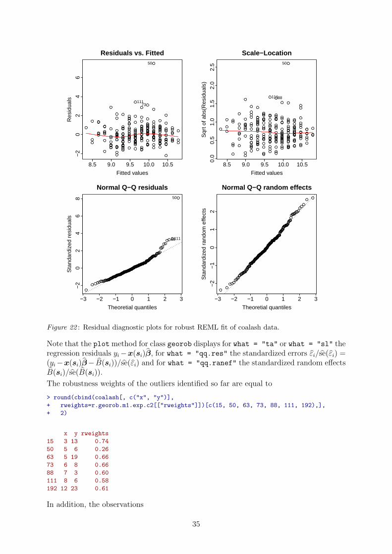
Figure 22 : Residual diagnostic plots for robust REML fit of coalash data.

Note that the plotmethod for class georob displays for what = "ta" or what = "sl" theregression residuals yi−x(si)β, for what = "qq.res" the standardized errors εi/se(εi) =(yi−x(si)β− B(si))/se(εi) and for what = "qq.ranef" the standardized random effectsB(si)/se(B(si)).

The robustness weights of the outliers identified so far are equal to

> round(cbind(coalash[, c("x", "y")],

+ rweights=r.georob.m1.exp.c2[["rweights"]])[c(15, 50, 63, 73, 88, 111, 192),],

+ 2)

x y rweights

15 3 13 0.74

50 5 6 0.26

63 5 19 0.66

73 6 8 0.66

88 7 3 0.60

111 8 6 0.58

192 12 23 0.61

In addition, the observations

35

> sel <- r.georob.m1.exp.c2[["rweights"]] <= 0.8 &

+ !1:nrow(coalash) %in% c(15, 50, 63, 73, 88, 111, 192)

> round(cbind(coalash[, c("x", "y")],

+ rweights=r.georob.m1.exp.c2[["rweights"]])[sel,],

+ 2)

x y rweights

20 3 8 0.70

157 10 14 0.73

171 11 10 0.72

173 11 12 0.80

have weights ≤ 0.8. All these outliers are marked in Figure 23 by ×:

> plot(y~x, coalash, cex=sqrt(abs(residuals(r.georob.m1.exp.c2))),

+ col=c("blue", NA, "red")[sign(residuals(r.georob.m1.exp.c2))+2], asp=1,

+ main="estimated errors robust REML", xlab="northing", ylab="easting")

> points(y~x, coalash, subset=r.georob.m1.exp.c2[["rweights"]]<=0.8, pch=4); grid()

> legend("topleft", pch=1, col=c("blue", "red"), legend=c("< 0", "> 0"), bty="n")

5 10 15

05

1015

2025

estimated errors robust REML

northing

east

ing

< 0> 0

Figure 23 : “Bubble plot” of independent errors ε estimated by robust REML (area of symbols

∝ moduli of residuals; ×: observation with robustness weights wi ≤ 0.8).

Comparison with Figure 15 reveals that the 5 additional mild outliers were visible in thisplot as well, but were not identified by Cressie’s exploratory analysis.

36

For comparison, we fit the same model by Gaussian REML by setting the tuning constantof the ψc-function c ≥ 1000:

> r.georob.m1.exp.c1000 <- update(r.georob.m1.exp.c2, tuning.psi=1000)

> summary(r.georob.m1.exp.c1000)

Call:georob(formula = coalash ~ x, data = coalash, locations = ~x +

y, variogram.model = "RMexp", param = c(variance = 0.1, nugget = 0.9,

scale = 1), tuning.psi = 1000)




eta scale

Gradient : -1.2256e-02 2.3135e-02

Maximized restricted log-likelihood: -319.51



-0.6332 -0.1703 -0.0198 0.1814 1.3713



-2.121 -0.612 -0.107 0.405 6.068



-2.284 -0.658 -0.115 0.434 6.500

Gaussian REML estimates

Variogram: RMexp


variance 0.2675 0.0745 0.96


nugget 1.0225 0.7151 1.46

scale 1.9067 0.3017 12.05



(Intercept) 10.9848 0.3218 34.1 < 2e-16 ***

x -0.1629 0.0371 -4.4 1.8e-05 ***

---

Signif. codes: 0 '***' 0.001 '**' 0.01 '*' 0.05 '.' 0.1 ' ' 1


Robustness weights:

All 208 weights are ~= 1.

37

and compare the Gaussian and robust REML estimates of the variogram:

> plot(r.georob.m1.exp.c1000, lag.dist.def=1, max.lag=10, estimator="matheron")

> plot(r.georob.m1.exp.c2, lag.dist.def=1, max.lag=10, estimator="qn", add = TRUE,

+ col="blue")

> plot(update(r.georob.m1.exp.c2, subset=-50), lag.dist.def=1, max.lag=10, estimator="qn",

+ add = TRUE, col="orange")

> legend("bottomright", lt=1, col=c("black","blue", "orange"),

+ legend =c("Gaussian REML", "robust REML", "Gaussian REML without outlier (5,6)" ), bty="n")

0 2 4 6 8

0.0

0.2

0.4

0.6

0.8

1.0

1.2

1.4

lag distance

sem

ivar

ianc

e

Gaussian REMLrobust REMLGaussian REML without outlier (5,6)

Figure 24 : Gaussian and robust REML estimate of exponential variogram.

The outliers inflate mostly the nugget effect (by ≈ 20 %) and less so the signal varianceand range parameter (by ≈ 10 %). When we eliminate the severest outlier at (5,6) thenthe Gaussian and robust REML estimates of the variogram hardly differ.

Gaussian REML masks the estimated independent errors (εi) somewhat at the cost ofinflated estimates of random effects (B(si)):

> op <- par(mfrow=c(1,2), cex=5/6)

> plot(residuals(r.georob.m1.exp.c2), residuals(r.georob.m1.exp.c1000),

+ asp = 1, main=expression(paste("Gaussian vs robust ", widehat(epsilon))),

+ xlab=expression(paste("robust ", widehat(epsilon))),

+ ylab=expression(paste("Gaussian ", widehat(epsilon))))


> plot(ranef(r.georob.m1.exp.c2), ranef(r.georob.m1.exp.c1000),

+ asp = 1, main=expression(paste("Gaussian vs robust ", italic(widehat(B)))),

+ xlab=expression(paste("robust ", italic(widehat(B)))),

+ ylab=expression(paste("Gaussian ", italic(widehat(B)))))


38

−2 0 2 4 6

−2

02

46

Gaussian vs robust ε

robust ε

Gau

ssia

n ε

−1.0 −0.5 0.0 0.5 1.0

−0.

50.

00.

51.

0

Gaussian vs robust B

robust B

Gau

ssia

n B

Figure 25 : Comparison of estimated errors εi and random effects B(si) for Gaussian and robust

REML fit of coalash data.

We compare the Gaussian and robust REML fit by 10-fold cross-validation:

> r.cv.georob.m1.exp.c2 <- cv(r.georob.m1.exp.c2, seed=1)


Warning message:

In cv.georob(r.georob.m1.exp.c2, seed = 1, ) :

lack of covergence for 1 cross-validation sets

The robustfied estimating equations could not be solved for one cross-valiation subset.This may happen if the initial guesses of the variogram parameters are too far awayfrom the root (see section 5.7). Sometimes it helps then to suppress the computation ofrobust guesses of the variogram parameters and to use the robust parameter estimatescomputed from the whole data set as initial values (see argument initial.param ofcontrol.georob() and section 5.7):

> r.cv.georob.m1.exp.c2 <- cv(r.georob.m1.exp.c2, seed=1,

+ control=control.georob(initial.param=FALSE))


By default, cv.georob() partitions the data set into 10 geographically compact subsetsof adjacent locations (see argument method of cv.georob() and section 7.3):

> plot(y~x, r.cv.georob.m1.exp.c2$pred, asp=1, col=subset, pch=as.integer(subset))

39

5 10 15

05

1015

2025

x

y

Figure 26 : Default method for defining cross-validation subsets by kmeans() using argument

method="block" of cv.georob().

We compute now summary statistics of the (standardized) cross-validation predictionerrors for the two model fits (see section 7.3):

> summary(r.cv.georob.m1.exp.c1000, se=TRUE)



-0.00619 -0.09188 1.13358 1.05789 0.99910 1.08170 0.38084

se 0.12310 0.12965 0.11588 0.07763 0.05409 0.34814 0.06354

crps

0.60090

se 0.04566

> summary(r.cv.georob.m1.exp.c2, se=TRUE)



0.0441 -0.0659 1.1260 1.0427 0.9819 1.2392 0.4568 0.5920

se 0.1127 0.1235 0.1167 0.0693 0.0554 0.3318 0.0704 0.0471

40

The statistics of cross-validation errors are marginally better for the robust fit.

For robust REML, the standard errors of the cross-validation errors are likely too small.This is due to the fact that for the time being, the Kriging variance of the response Yis approximated by adding the estimated nugget τ 2 to the Kriging variance of the signalZ. This approximation likely underestimates the mean squared prediction error of theresponse if the errors come from a long-tailed distribution. Hence, the summary statisticsof the standardized prediction errors (msse, medsse) should be interpreted with caution.The same is true for the continuous-ranked probability score (crps), which is computedunder the assumption that the predictive distribution of Y is Gaussian even if the errorscome from a long-tailed distribution. This cannot strictly hold.

For illustration, we nevertheless show here some diagnostics plots of criteria of the cross-validation prediction errors that further depend on the predictive distributions of theresponse:

> op <- par(mfrow=c(3, 2))

> plot(r.cv.georob.m1.exp.c2, type="ta", col="blue")

> plot(r.cv.georob.m1.exp.c1000, type="ta", col="orange", add=TRUE)

> abline(h=0, lty="dotted")

> legend("topleft", pch=1, col=c("orange", "blue"), legend=c("Gaussian", "robust"), bty="n")

> plot(r.cv.georob.m1.exp.c2, type="qq", col="blue")

> plot(r.cv.georob.m1.exp.c1000, type="qq", col="orange", add=TRUE)


> legend("topleft", lty=1, col=c("orange", "blue"), legend=c("Gaussian", "robust"), bty="n")

> plot(r.cv.georob.m1.exp.c2, type="ecdf.pit", col="blue", do.points=FALSE)

> plot(r.cv.georob.m1.exp.c1000, type="ecdf.pit", col="orange", add=TRUE, do.points=FALSE)


> legend("topleft", lty=1, col=c("orange", "blue"), legend=c("Gaussian", "robust"), bty="n")

> plot(r.cv.georob.m1.exp.c2, type="bs", col="blue")

> plot(r.cv.georob.m1.exp.c1000, type="bs", col="orange", add=TRUE)

> legend("topright", lty=1, col=c("orange", "blue"), legend=c("Gaussian", "robust"), bty="n")

> plot(r.cv.georob.m1.exp.c1000, type="mc", main="Gaussian REML")

> plot(r.cv.georob.m1.exp.c2, type="mc", main="robust REML")

> par(op)

41

8.5 9.0 9.5 10.0 10.5 11.0

−2

02

46

Tukey−Anscombe plot

predictions

stan

dard

ized

pre

dict

ion

erro

rsGaussianrobust

−3 −2 −1 0 1 2 3

−2

02

46

normal−QQ−plot of standardized prediction errors

quantile N(0,1)

quan

tiles

of s

tand

ardi

zed

pred

ictio

n er

rors

Gaussianrobust

0.0 0.2 0.4 0.6 0.8 1.0

0.0

0.2

0.4

0.6

0.8

1.0

ecdf PIT−values

PIT

prob

abili

ty

Gaussianrobust

8 10 12 14 16 18

0.00

0.05

0.10

0.15

0.20

Brier score vs. cutoff

cutoff

Brie

r sc

ore

Gaussianrobust

8 10 12 14 16 18

0.0

0.2

0.4

0.6

0.8

1.0

Gaussian REML

data or predicitons

prob

abili

ty

−0.

04−

0.02

0.00

0.02

empirical cdf Gmean predictive cdf F

F − G

8 10 12 14 16 18

0.0

0.2

0.4

0.6

0.8

1.0

robust REML

data or predicitons

prob

abili

ty

−0.

02−

0.01

0.00

0.01

0.02empirical cdf G

mean predictive cdf F

F − G

Figure 27 : Diagnostic plots of the standardized cross-validation errors, the probability integral

transform (PIT), the Brier score and of the predictive distributions for Gaussian and robust

REML.

In general, the diagnostics are slightly better for robust than for Gaussian REML: Theempirical distribution of the probability integral transform (PIT) is closer to a uniform

42

distribution, the Brier score (BS) is smaller and the average predictive distribution F iscloser to the empirical distribution of the data G (see section 7.3 and Gneiting et al.,2007, for more details about the interpretation of these plots).

4.3 Computing robust Kriging predictions

4.3.1 Point Kriging

For point Kriging we must first generate a fine-meshed grid of predictions points(optionally with the covariates for the drift) that is passed as argument newdata

to predict.georob(). newdata can be an customary data.frame, an object ofclass SpatialPointsDataFrame, SpatialPixelsDataFrame or SpatialGridDataFrame

or SpatialPoints, SpatialPixels or SpatialGrid, all provided by the package sp. Ifnewdata is a SpatialPoints, SpatialPixels or a SpatialGrid object then the driftmodel may only use the coordinates as covariates (universal Kriging), as we do it here.

> coalash.grid <- expand.grid(x=seq(-1, 17, by=0.2),

+ y=seq( -1, 24, by=0.2))

> coordinates( coalash.grid) <- ~x+y # convert to SpatialPoints

> gridded( coalash.grid) <- TRUE # convert to SpatialPixels

> fullgrid( coalash.grid) <- TRUE # convert to SpatialGrid

> str(coalash.grid, max=2)

Formal class 'SpatialGrid' [package "sp"] with 3 slots

..@ grid :Formal class 'GridTopology' [package "sp"] with 3 slots

..@ bbox : num [1:2, 1:2] -1.1 -1.1 17.1 24.1



Computing (robust) plug-in Kriging predictions is then straightforward:

> r.pk.m1.exp.c2 <- predict(r.georob.m1.exp.c2, newdata=coalash.grid)

> r.pk.m1.exp.c1000 <- predict(r.georob.m1.exp.c1000, newdata=coalash.grid)

and plotting the results by the function spplot() of the package sp as well:

> pred.rob <- spplot(r.pk.m1.exp.c2, "pred", at=seq(8, 12, by=0.25),

+ main="robust Kriging prediction", scales=list(draw=TRUE))

> pred.gauss <- spplot(r.pk.m1.exp.c1000, "pred", at=seq(8, 12, by=0.25),

+ main="Gaussian Kriging prediction", scales=list(draw=TRUE))

> se.rob <- spplot(r.pk.m1.exp.c2, "se", at=seq(0.35, 0.65, by=0.025),

+ main="standard error robust Kriging", scales=list(draw=TRUE))

> se.gauss <- spplot(r.pk.m1.exp.c1000, "se", at=seq(0.35, 0.65, by=0.025),

+ main="standard error Gaussian Kriging", scales=list(draw=TRUE))

> plot(pred.rob, pos=c(0, 0.5, 0.5, 1), more=TRUE)

> plot(pred.gauss, pos=c(0.5, 0.5, 1, 1), more=TRUE)

> plot(se.rob, pos=c(0, 0, 0.5, 0.5), more=TRUE)

> plot(se.gauss, pos=c(0.5, 0, 1, 0.5), more=FALSE)

43

robust Kriging prediction

0

5

10

15

20

0 5 10 15

8.0

8.5

9.0

9.5

10.0

10.5

11.0

11.5

12.0

Gaussian Kriging prediction

0

5

10

15

20

0 5 10 15

8.0

8.5

9.0

9.5

10.0

10.5

11.0

11.5

12.0

standard error robust Kriging

0

5

10

15

20

0 5 10 15

0.35

0.40

0.45

0.50

0.55

0.60

0.65

standard error Gaussian Kriging

0

5

10

15

20

0 5 10 15

0.35

0.40

0.45

0.50

0.55

0.60

0.65

Figure 28 : Robust (left) and Gaussian (right) point Kriging predictions (top) and Kriging

standard errors (bottom).

By default, predict.georob() predicts the signal Z(s), but predictions of the response

Y (s) or estimates of model terms and trend (drift) can be computed as well (see argu-ment type of predict.georob() and section 6.1.1). Apart from Kriging predictions andstandard errors, bounds (lower, upper) of point-wise 95%-prediction intervals (plug-in)are computed for assumed Gaussian predictive distributions.

The Kriging predictions visibly differ around the outlier at (5,6) and the Kriging stan-dard errors are larger for Gaussian Kriging because the outliers inflated the non-robustlyestimated sill of the variogram (Figure 24). To see the effects of outliers more clearly, weplot the relative difference of Gaussian and robust Kriging predictions and the ratio ofthe respective Kriging variances:

> library(lattice)

> # rel. difference of predictions

> r.pk.m1.exp.c2$reldiff.pred <- (r.pk.m1.exp.c1000$pred -

44

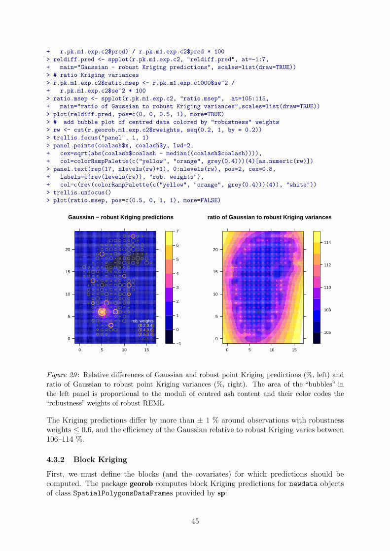
+ r.pk.m1.exp.c2$pred) / r.pk.m1.exp.c2$pred * 100

> reldiff.pred <- spplot(r.pk.m1.exp.c2, "reldiff.pred", at=-1:7,

+ main="Gaussian - robust Kriging predictions", scales=list(draw=TRUE))

> # ratio Kriging variances

> r.pk.m1.exp.c2$ratio.msep <- r.pk.m1.exp.c1000$se^2 /

+ r.pk.m1.exp.c2$se^2 * 100

> ratio.msep <- spplot(r.pk.m1.exp.c2, "ratio.msep", at=105:115,

+ main="ratio of Gaussian to robust Kriging variances",scales=list(draw=TRUE))

> plot(reldiff.pred, pos=c(0, 0, 0.5, 1), more=TRUE)

> # add bubble plot of centred data colored by "robustness" weights

> rw <- cut(r.georob.m1.exp.c2$rweights, seq(0.2, 1, by = 0.2))

> trellis.focus("panel", 1, 1)

> panel.points(coalash$x, coalash$y, lwd=2,

+ cex=sqrt(abs(coalash$coalash - median((coalash$coalash)))),

+ col=colorRampPalette(c("yellow", "orange", grey(0.4)))(4)[as.numeric(rw)])

> panel.text(rep(17, nlevels(rw)+1), 0:nlevels(rw), pos=2, cex=0.8,

+ labels=c(rev(levels(rw)), "rob. weights"),

+ col=c(rev(colorRampPalette(c("yellow", "orange", grey(0.4)))(4)), "white"))

> trellis.unfocus()

> plot(ratio.msep, pos=c(0.5, 0, 1, 1), more=FALSE)

Gaussian − robust Kriging predictions

0

5

10

15

20

0 5 10 15

−1

0

1

2

3

4

5

6

7

(0.8,1](0.6,0.8](0.4,0.6](0.2,0.4]

rob. weights

ratio of Gaussian to robust Kriging variances

0

5

10

15

20

0 5 10 15

106

108

110

112

114

Figure 29 : Relative differences of Gaussian and robust point Kriging predictions (%, left) and

ratio of Gaussian to robust point Kriging variances (%, right). The area of the “bubbles” in

the left panel is proportional to the moduli of centred ash content and their color codes the

“robustness” weights of robust REML.

The Kriging predictions differ by more than ± 1 % around observations with robustnessweights ≤ 0.6, and the efficiency of the Gaussian relative to robust Kriging varies between106–114 %.

4.3.2 Block Kriging

First, we must define the blocks (and the covariates) for which predictions should becomputed. The package georob computes block Kriging predictions for newdata objectsof class SpatialPolygonsDataFrames provided by sp:

45

> tmp <- expand.grid(x = seq(2.5, 16.5, by=4), y=seq(2, 22, by=4))

> rownames(tmp) <- paste("block", rownames(tmp), sep="")

> # create SpatialPolygonsDataFrame

> coalash.polygons <- sapply(1:nrow(tmp), function(i, x){

+ Polygons(list(Polygon(

+ t(x[,i] + t(cbind(c(-2, 2, 2, -2, -2), c(-2, -2, 2, 2, -2)))),

+ hole=FALSE)), ID=paste("block", i, sep=""))},

+ x=t(tmp))

> coalash.polygons <- SpatialPolygonsDataFrame(SpatialPolygons(coalash.polygons),

+ data = tmp)

> summary(coalash.polygons)

Object of class SpatialPolygonsDataFrame

Coordinates:

min max

x 0.5 16.5

y 0.0 24.0

Is projected: NA

proj4string : [NA]

Data attributes:

x y

Min. : 2.5 Min. : 2

1st Qu.: 5.5 1st Qu.: 6

Median : 8.5 Median :12

Mean : 8.5 Mean :12

3rd Qu.:11.5 3rd Qu.:18

Max. :14.5 Max. :22

> plot(coalash.polygons, col="grey", axes=TRUE); points(y~x, coalash)

0 5 10 15

05

1015

2025

Figure 30 : Geometry of blocks for which Kriging predictions are computed (dots are data

locations).

46

Note that coordinates of the block centres are the covariates for the drift model of theblock means. Block-block- and point-block-means of the semi-variance are computed bypredict.georob() efficiently by functions of the R packages constrainedKriging andspatialCovariance (see section 6.1 and Hofer and Papritz, 2011; Clifford, 2005):

> r.bk.m1.exp.c2 <- predict(r.georob.m1.exp.c2, newdata=coalash.polygons,

+ control=control.predict.georob(pwidth=4, pheight=4, full.covmat=TRUE))

> r.bk.m1.exp.c1000 <- predict(r.georob.m1.exp.c1000, newdata=coalash.polygons,

+ control=control.predict.georob(pwidth=4, pheight=4, full.covmat=TRUE))

Since the blocks are squares of constant size, choosing a square “integration pixel” of thesame dimension (arguments pwidth, pheight of control.predict.georob()) allows tocompute the required mean semi-variances most efficiently (see Hofer and Papritz, 2011,for details). The third argument full.covmat=TRUE of control.predict.georob() hasthe effect that the full covariance matrix of the predictions errors of the block means iscomputed (and stored as list component mse.pred in r.bk.m1.exp.c2):

> str(r.bk.m1.exp.c2, max=2)

List of 2

$ pred :Formal class 'SpatialPolygonsDataFrame' [package "sp"] with 5 slots

$ mse.pred: num [1:24, 1:24] 0.08216 0.01212 -0.00303 -0.01803 0.02881 ...

We can compute from these covariances the Kriging variances of the spatial means overgroups of block, in particular of the spatial mean over the whole domain:

> c(pred=mean(r.bk.m1.exp.c2$pred$pred),

+ se=sqrt(sum(r.bk.m1.exp.c2$mse.pred))/24)

pred se

9.558919 0.087422

which is of course the same as predicting the mean over the whole domain by blockKriging:

> coalash.domain <- rbind(c(0.5,0), c(16.5,0), c(16.5,24), c(0.5,24), c(0.5,0))

> coalash.domain <- SpatialPolygonsDataFrame(

+ SpatialPolygons(list(Polygons(list(Polygon(coalash.domain)), ID= "domain"))),

+ data=data.frame(x=8.5,y=12,row.names="domain"))

> slot(predict(r.georob.m1.exp.c2, newdata=coalash.domain,

+ control=control.predict.georob(pwidth=16, pheight=24)), "data")

pred se lower upper

domain 9.5589 0.087422 9.3876 9.7303

We conclude this section by graphs of the robust and Gaussian block Kriging predictions:

> pred.rob <- spplot(r.bk.m1.exp.c2$pred, "pred", at=seq(8, 11, by=0.25),

+ main="robust Kriging prediction", scales=list(draw=TRUE))

> pred.gauss <- spplot(r.bk.m1.exp.c1000$pred, "pred", at=seq(8, 11, by=0.25),

+ main="Gaussian Kriging prediction", scales=list(draw=TRUE))

> se.rob <- spplot(r.bk.m1.exp.c2$pred, "se", at=seq(0.15, 0.45, by=0.025),

+ main="standard error robust Kriging", scales=list(draw=TRUE))

> se.gauss <- spplot(r.bk.m1.exp.c1000$pred, "se", at=seq(0.15, 0.45, by=0.025),

+ main="standard error Gaussian Kriging", scales=list(draw=TRUE))

> plot(pred.rob, pos=c(0, 0.5, 0.5, 1), more=TRUE)

> plot(pred.gauss, pos=c(0.5, 0.5, 1, 1), more=TRUE)

> plot(se.rob, pos=c(0, 0, 0.5, 0.5), more=TRUE)

> plot(se.gauss, pos=c(0.5, 0, 1, 0.5), more=FALSE)

47

robust Kriging prediction

5

10

15

20

5 10 15

8.0

8.5

9.0

9.5

10.0

10.5

11.0

Gaussian Kriging prediction

5

10

15

20

5 10 15

8.0

8.5

9.0

9.5

10.0

10.5

11.0

standard error robust Kriging

5

10

15

20

5 10 15

0.15

0.20

0.25

0.30

0.35

0.40

0.45

standard error Gaussian Kriging

5

10

15

20

5 10 15

0.15

0.20

0.25

0.30

0.35

0.40

0.45

Figure 31 : Robust (left) and Gaussian (right) block Kriging predictions (top) and Kriging

standard errors (bottom).

The outlier at (5,6) also affects the the prediction of the block means and robust blockKriging is again more efficient than Gaussian block Kriging.

48

5 Details about parameter estimation

5.1 Implemented variogram models

Currently, estimation of the parameters of the following models is implemented (see ar-gument variogram.model of georob()):"RMaskey", "RMbessel", "RMcauchy", "RMcircular", "RMcubic", "RMdagum","RMdampedcos", "RMdewijsian", "RMexp" (default), "RMfbm", "RMgauss","RMgencauchy", "RMgenfbm", "RMgengneiting", "RMgneiting", "RMlgd", "RMmatern","RMpenta", "RMqexp", "RMspheric", "RMstable", "RMwave", "RMwhittle".

Some of these models have in addition to variance, snugget, nugget and scale furtherparameters. Initial values of these parameters (param) and fitting flags (fit.param)must be passed to georob() by the same names as used by the functions RM...() ofthe package RandomFields (see RMmodel()). Use the function param.names() to listadditional parameters of a given variogram.model.

The arguments fit.param and fit.aniso are used to control what variogram andanisotropy parameters are estimated and which are kept at the constant initial values.The functions default.fit.param() and default.fit.aniso() set reasonable defaultvalues for these arguments. Note, as an aside, that the function default.aniso() sets(default) values of the anisotropy parameters for an isotropic variogram.

5.2 Estimating parameters of power function variogram

The intrinsic variogram model RMfbm is over-parametrized when both the variance

(plus possibly snugget) and the scale are estimated. Therefore, to estimate theparameters of this model, scale must be kept fixed at an arbitrary value by usingfit.param = default.fit.param(scale = FALSE).

5.3 Estimating parameters of geometrically anisotropic vari-ograms

Subsection 2.1 describes how covariances are modelled in general. Here we describe indetail how geometrically anisotropic variogram are parametrized:

The matrix A = A(α, f1, f2;ω, φ, ζ) (see equation 4) maps an arbitrary point on anellipsoidal surface with constant (generalized) covariance in IR3, centred on the origin,and having lengths of semi-principal axes, p1, p2, p3, equal to |p1| = α, |p2| = f1 α and|p3| = f2 α, 0 < f2 ≤ f1 ≤ 1, respectively, onto the surface of the unit ball centred on theorigin. The orientation of the ellipsoid is defined by the three angles ω, φ and ζ:

ω is the azimuth of p1 (= angle between north and the projection of p1 onto the x-y-plane,measured from north to south positive clockwise in degrees),

φ is 90 degrees minus the altitude of p1 (= angle between the zenith and p1, measuredfrom zenith to nadir positive clockwise in degrees), and

ζ is the angle between p2 and the direction of the line, say y′, defined by the intersectionbetween the x-y-plane and the plane orthogonal to p1 running through the origin(ζ is measured from y′ positive counter-clockwise in degrees).

49

The transformation matrix is given by

A =

1/α 0 00 1/(f1 α) 00 0 1/(f2 α)

(C1,C2,C3) (8)

where

CT1 = (sinω sinφ,− cosω cos ζ − sinω cosφ sin ζ, cosω sin ζ − sinω cosφ cos ζ)

CT2 = (cosω sinφ, sinω cos ζ − cosω cosφ sin ζ,− sinω sin ζ − cosω cosφ cos ζ)

CT3 = (cosφ, sinφ sin ζ, sinφ cos ζ) (9)

To model geometrically anisotropic variograms in IR2 one has to set φ = 90 and f2 = 1, andfor f1 = f2 = 1 one obtains the model for isotropic auto-correlation with range parameterα. Note that for isotropic auto-correlation the software processes data for which d mayexceed 3.

Some additional remarks might be helpful:

• The first semi-principal axis points into the direction with the farthest reachingauto-correlation, which is described by the range parameter scale (α).

• The ranges in the direction of the second and third semi-principal axes are given byf1α and f2α, with 0 < f2 ≤ f1 ≤ 1.

• The default values for aniso (f1 = 1, f2 = 1) define an isotropic variogram model.

• Valid ranges for the angles characterizing the orientation of the semi-variance ellip-soid are (in degrees): ω [0, 180], φ [0, 180], ζ [-90, 90].

5.4 Estimating variance of micro-scale variation

Simultaneous estimation of the variance of the micro-scale variation (snugget, σ2n), which

appears seemingly as spatially uncorrelated with a given sampling design, and of the vari-ance (nugget, τ 2) of the independent errors requires that for some locations si replicatedobservations are available. Locations less or equal than zero.dist apart are therebyconsidered as being coincident (see control.georob()).

5.5 Estimating variance parameters by Gaussian (RE)ML

Unlike robust REML, where robustified estimating equations are solved for the varianceparameters nugget (τ 2), variance (σ2), and possibly snugget (σ2

n), for Gaussian (RE)MLthe variances can be re-parametrized to

• the signal variance σ2Z = σ2 + σ2

n,

• the inverse relative nugget η = σ2Z/τ

2 and

• the relative auto-correlated signal variance ξ = σ2/σ2Z .

georob() maximizes then a (restricted) profile log-likelihood that depends only on η, ξ,α, . . . , and σ2

Z is estimated by an explicit expression that depends on these parameters(e.g. Diggle and Ribeiro, 2007, p. 113). This is usually more efficient than maximizingthe (restricted) log-likelihood with respect to the original variance parameters τ 2, σ2

n andσ2. georob() chooses the parametrization automatically, but the user can control it bythe argument reparam of the function control.georob().

50

5.6 Constraining estimates of variogram parameters

Parameters of variogram models can vary only within certain bounds (see param.bounds()and RMmodel() for allowed ranges). georob() uses three mechanisms to constrain param-eter estimates to permissible ranges:

1. Parameter transformations : By default, all variance (variance, snugget, nugget),the range scale and the anisotropy parameters f1 and f2 are log-transformed beforesolving the estimating equations or maximizing the restricted log-likelihood andthis warrants that the estimates are always positive (see control.georob() andsection 5.9.4 for detailed explanations how to control parameter transformations).

2. Checking permissible ranges : The additional parameters of the variogram modelssuch as the smoothness parameter ν of the Whittle-Matern model are forced to stayin the permissible ranges by signalling an error to nleqslv(), nlminb() or optim()if the current trial values are invalid. These functions then graciously update thetrial values of the parameters and carry their task on. However, it is clear that sucha procedure likely gets stuck at a point on the boundary of the parameter space andis therefore just a workaround for avoiding runtime errors due to invalid parametervalues.

3. Exploiting the functionality of nlminb() and optim(): If a spatial model is fittednon-robustly, then the arguments lower, upper (and method of optim()) canbe used to constrain the parameters (see control.optim() how to pass them tooptim()). For optim() one has to use the arguments method = "L-BFGS-B",lower = l, upper = u, where l and u are numeric vectors with the lowerand upper bounds of the transformed parameters in the order as they appear inc(variance, snugget, nugget, scale, ...)[fit.param], aniso[fit.aniso]),where ... are additional parameters of isotropic variogram models (useparam.names(variogram.model) to display the names and the order of theadditional parameters for variogram.model).

5.7 Computing robust initial estimates of parameters for robustREML

To solve the robustified estimating equations for B and β the following initial estimatesare used:

• B = 0, if this turns out to be infeasible, initial values can be passed to georob()

by the argument bhat of control.georob().

• β is either estimated robustly by the function lmrob(), rq() or non-robustly bylm() (see argument initial.fixef of control.georob()).

Finding the roots of the robustified estimating equations of the variogram and anisotropyparameters is more sensitive to a good choice of initial values than maximizing the Gaus-sian (restricted) log-likelihood with respect to the same parameters. If the initial valuesfor param and aniso are not sufficiently close to the roots of the system of nonlinearequations, then nleqslv() may fail to find them. Setting initial.param = TRUE allowsone to find initial values that are often sufficiently close to the roots so that nleqslv()converges. This is achieved by:

51

1. Initial values of the regression parameters are computed by lmrob() irrespective ofthe choice for initial.fixef (see control.georob()).

2. Observations with“robustness weights”of the lmrob fit, satisfying ψc(εi/τ)/(εi/τ) ≤min.rweight, are discarded (see control.georob()).

3. The model is fit to the pruned data set by Gaussian REML using optim() ornlminb().

4. The resulting estimates of the variogram parameters (param, aniso) are used asinitial estimates for the subsequent robust fit of the model by nleqslv().

Note that for step 3 above, initial values of param (and possibly aniso) must be providedto georob().

5.8 Estimating parameters of “nested” variogram models

As a further option, georob() allows to estimate parameters of so-called “nested” vari-ogram models. For this one assumes that the signal process Z(s) is the sum of severalindependent auto-correlated Gaussian processes Bk(s)

B(s) =K∑

k=1

Bk(s), (10)

each characterized by a parametric variogram function with parameters (σ2Z,k, θk), see

equation 3. Initial values for nested variogram models are passed to georob() by theargument variogram.object, which must be a list of length K. The kth component ofvariogram.object is itself a list with the mandatory components variogram.model andparam and the optional components fit.param, aniso and fit.aniso. Note that sensibledefaults are used if the optional components are missing. Note further that nugget andsnugget may be specified for all k model strctures but these variances are summed-upand assigned to the first model structure (k = 1) and all nugget and snugget are set tozero for k > 1.

5.9 Controlling georob() by the function control.georob()

All control and tuning parameters except the robustness tuning constant c of the ψc-function (argument tuning.psi of georob()) are set by the arguments of the functioncontrol.georob(), which generates a list that is passed by the control argument togeorob(). This section describes in some detail how to control georob() by the variousarguments of control.georob().

5.9.1 Gaussian (RE)ML estimation

Gaussian (RE)ML estimates are computed provided tuning.psi ≥ 1000. Use the ar-gument ml.method to select either "ML" or "REML" (default) and the argument reparamto control whether the re-parametrized (default TRUE) or the original variogram param-eters are estimated (see section 5.5). The function used to maximize the (restricted)log-likelihood is chosen by the argument maximizer (default "nlminb"). Use the argu-ment nlminb along with the function control.nlminb() (or the argument optim along

52

with control.optim() to pass arguments to nlminb() (or optim()), in particular theargument rel.tol, which controls convergence. The argument hessian controls whetherconfidence intervals of variogram parameters are computed from the observed Fisher infor-mation based on the asymptotic normal distribution of (RE)ML estimates (default TRUE,see summary.georob()).

5.9.2 Robust REML estimation

The argument psi.func selects the ψc-function for robust REML. Apart from a shiftedand scaled logistic CDF

ψc(x) = tanh(x/c)

("logistic", default), the Huber ("huber") or a re-descending ψc-function based on thet-distribution ("t.dist")

ψc(x) =c2 x

c2 + x2

can be used.The argument initial.fixef chooses the function for computing (robust) initial es-timates of β. Possible choices are "lmrob" (default) "rq" and "lm". Use the argu-ment lmrob along with the function lmrob.control() (or the argument rq along withthe function control.rq() to pass arguments to lmrob() (or rq()). The argumentinitial.param controls whether robust initial estimates of the variogram parameters arecomputed (default TRUE, see section 5.7).For given variogram parameters, the estimating equations for β and B are solved byiterated re-weighted least squares (IRWLS). The argument irwls.maxiter sets the max-imum number of iterations (default 50), and the argument irwls.ftol controls conver-gence: Convergence is assumed if the largest absolute function value at the current rootis less than irwls.ftol (default 10−5). The current estimates β and B are then pluggedinto the estimating equations for θ and τ 2 that are solved in turn by nleqslv(). Usethe argument nleqslv along with the function control.nleqslv() to pass arguments tonleqslv(), in particular ftol, which controls convergence for root finding.

5.9.3 Approximation of covariances of fixed and random effects and residuals

The robustified estimating equations of robust REML depend on the covariances ofB. These covariances (and the covariances of B − B, β, ε, ε + B) are approxi-mated by expressions that in turn depend on the variances of ε, ψc(ε/τ) and the ex-pectation of ψ′

c(ε/τ) (= ∂/∂εψc(ε/τ)). The arguments error.family.estimation,error.family.cov.effects and error.family.cov.residuals of control.georob()control what parametric distribution for ε is used to compute the variances of ε, ψc(ε/τ)and the expectation of ψ′

c(ε/τ) when

• solving the estimating equations (error.family.estimation),

• computing the covariances of β, B and B − B (error.family.cov.effects) and

• computing the covariances of ε = Y − Xβ − B and ε + B = Y − Xβ

(error.family.cov.residuals).

53

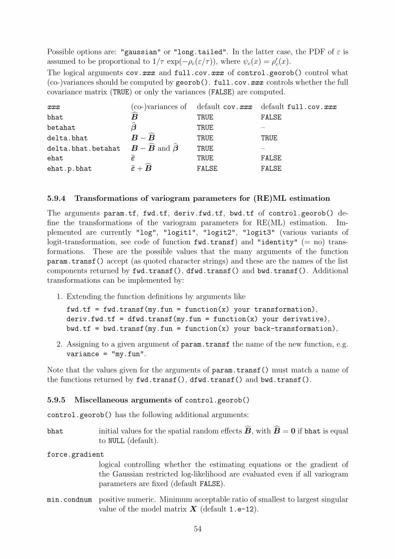
Possible options are: "gaussian" or "long.tailed". In the latter case, the PDF of ε isassumed to be proportional to 1/τ exp(−ρc(ε/τ)), where ψc(x) = ρ′c(x).

The logical arguments cov.xxx and full.cov.xxx of control.georob() control what(co-)variances should be computed by georob(). full.cov.xxx controls whether the fullcovariance matrix (TRUE) or only the variances (FALSE) are computed.

xxx (co-)variances of default cov.xxx default full.cov.xxx

bhat B TRUE FALSE

betahat β TRUE –

delta.bhat B − B TRUE TRUE

delta.bhat.betahat B − B and β TRUE –ehat ε TRUE FALSE

ehat.p.bhat ε+ B FALSE FALSE

5.9.4 Transformations of variogram parameters for (RE)ML estimation

The arguments param.tf, fwd.tf, deriv.fwd.tf, bwd.tf of control.georob() de-fine the transformations of the variogram parameters for RE(ML) estimation. Im-plemented are currently "log", "logit1", "logit2", "logit3" (various variants oflogit-transformation, see code of function fwd.transf) and "identity" (= no) trans-formations. These are the possible values that the many arguments of the functionparam.transf() accept (as quoted character strings) and these are the names of the listcomponents returned by fwd.transf(), dfwd.transf() and bwd.transf(). Additionaltransformations can be implemented by:

1. Extending the function definitions by arguments like

fwd.tf = fwd.transf(my.fun = function(x) your transformation),deriv.fwd.tf = dfwd.transf(my.fun = function(x) your derivative),bwd.tf = bwd.transf(my.fun = function(x) your back-transformation),

2. Assigning to a given argument of param.transf the name of the new function, e.g.variance = "my.fun".

Note that the values given for the arguments of param.transf() must match a name ofthe functions returned by fwd.transf(), dfwd.transf() and bwd.transf().

5.9.5 Miscellaneous arguments of control.georob()

control.georob() has the following additional arguments:

bhat initial values for the spatial random effects B, with B = 0 if bhat is equalto NULL (default).

force.gradient

logical controlling whether the estimating equations or the gradient ofthe Gaussian restricted log-likelihood are evaluated even if all variogramparameters are fixed (default FALSE).

min.condnum positive numeric. Minimum acceptable ratio of smallest to largest singularvalue of the model matrix X (default 1.e-12).

54

zero.dist positive numeric equal to the maximum distance, separating two samplinglocations that are still considered as being coincident.

Note that georob() can fit models with rank-deficient model matrices. It uses then theMoore-Penrose inverse of the matrix XV −1

α,ξX to compute the projection matrices Aα

and P α (see Kunsch et al., in prep.).

5.10 Parallelized computations

Parallelized computations shorten computing time for large data sets (n > 1000).georob() and other functions of the package therefore use on non-windows OS the func-tion mclapply() (forking, package parallel) and on windows OS the functions parLapply(socket cluster, package parallel) as well as sfLapply() (socket cluster, package snowfall)for parallelized computations. The following tasks may be executed in parallel:

1. Simultaneously fitting multiple models by functions cv.georob(),profilelogLik() (section 7.2), add1.georob(), drop1.georob() andstep.georob() (section 7.1);

2. computing Kriging predictions by predict.georob() (section 6.1);

3. matrix multiplication by function pmm();

4. computing the (generalized) covariance matrix Γθ of the data by the (non-exported)function f.aux.gcr().

For tasks 1 and 2 the functions have an argument ncores to control how many cores shouldbe used for parallel computations. For tasks 3 and 4 one can use the argument pcmp

of control.georob() along with the function pcmp.control() to control parallelizedcomputations. The function pcmp.control() has the following arguments:

pmm.ncores number (integer, default 1) of cores used for parallelized matrix multipli-cation.

gcr.ncores number (integer, default 1) of cores used for parallelized computation of(generalized) covariance matrix.

max.ncores allowed maximum number of cores (integer, default all cores of a machine)used for parallelized computations.

f number (integer, default 2) of tasks assigned to each core in parallelizedcomputations.

sfstop logical controlling whether the SNOW socket cluster is stopped after eachparallelized computations on windows OS (default FALSE).

allow.recursive

logical controlling whether nested parallelized computation should be al-lowed (default TRUE).

55

Generating child processes requires itself resources and increasing the number of cores fortasks 3 and 4 does not always result in reduced computing time. A sensible default forthe number of cores for tasks 3 and 4 is likely 2. max.ncores controls how many childprocesses are generated in total. This can be used to prevent that child processes generatethemselves children which may result in too many child processes.

Note, however, that very substantial reductions in computing time results when one usesthe OpenBLAS library instead of the reference BLAS library that ships with R, seehttp://www.openblas.net/ and R FAQ for your OS. With OpenBLAS no gains areobtained by using more than one core for matrix multiplication, and one should thereforeuse the default argument pmm.ncores = 1 for control.pcmp().

56

http://www.openblas.net/

6 Details about Kriging

6.1 Functionality of predict.georob()

The predict method of class georob computes customary or robust external drift pointor block plug-in Kriging predictions (see equation 7). Data about the prediction targetsare passed as argument newdata to predict.georob(), where newdata can be either anordinary data frame, a SpatialPoints-, SpatialPixels-, SpatialGrid or a SpatialPolygons-

DataFrame, a SpatialPoints, SpatialPixels or a SpatialGrid object, all the latter providedby the package sp. If newdata is a SpatialPoints, SpatialPixels or a SpatialGrid ob-ject then the drift model may only use the coordinates as covariates (universal Kriging). Ifnewdata is a SpatialPolygonsDataFrame then block Kriging predictions are computed,otherwise point Kriging predictions.

6.1.1 Prediction targets

The argument type controls what quantities predict.georob() computes (given here fora target point s, but the same quantities are also computed for a block):

• "signal": the “signal”Z(s) = x(s)Tβ +B(s) of the process (default),

• "response": the observations Y (s) = Z(s) + ε(s),

• "trend": the external drift x(s)Tβ,

• "terms": the model terms. The argument terms can then be used to select theterms (default all terms) and se.fit controls whether standard errors of the termsare computed (default TRUE).

6.1.2 Further control

Use the argument control along with the function control.predict.georob() to fur-ther control what predict.georob() actually does:

Covariance matrices The argument full.covmat of control.predict.georob()

controls whether the full covariance matrices of prediction errors, fitted trend, etc. arecomputed (TRUE) or only the vector with their variances (FALSE, default).

Computing auxiliary items for log-normal Kriging Use the argumentextended.output = TRUE of control.predict.georob() to compute all quantities re-quired for the (approximately) unbiased back-transformation of Kriging predictions of log-transformed data to the original scale of the measurements by lgnpp() (see section 6.2).In more detail, the following items are computed:

• trend: the fitted values, x(s)Tβ,

• var.pred: the variances of the Kriging predictions, Varθ[Y (s)] or Varθ[Z(s)],

• cov.pred.target: the covariances between the predictions and the prediction tar-gets, Covθ[Y (s), Y (s)] or Covθ[Z(s), Z(s)],

• var.target: the variances of the prediction targets Varθ[Y (s)] or Varθ[Z(s)].

57

Note that the component var.pred is also present if type is equal to "trend", irrespectiveof the choice for extended.output. This component contains then the variances of thefitted values.

Contents and structure of returned object Depending on the values passed totype, full.covmat and extended.output, predict.georob() returns the following ob-ject:

1. If type is equal to "terms" then a vector, a matrix, or a list with prediction resultsalong with bounds and standard errors, see predict.lm().

2. If type is not equal to "terms" and full.covmat is FALSE thenthe result is an object of the same class as newdata (data frame,SpatialPointsDataFrame, SpatialPixelsDataFrame SpatialGridDataFrame,SpatialPolygonsDataFrame). The data frame or the data slot of theSpatialxxx DataFrame objects have the following components:

• the coordinates of the prediction points (only present if newdata is a dataframe).

• pred: the Kriging predictions (or fitted values).

• se: the root mean squared prediction errors (Kriging standard errors).

• lower, upper: the limits of tolerance/confidence intervals (the confidence levelis set by the argument signif) of predict.georob()),

• trend, var.pred, cov.pred.target, var.target: only present ifextended.output is TRUE, see above.

3. If type is not equal to "terms" and full.covmat is TRUE then predict.georob()

returns a list with the following components:

• pred: a data frame or a Spatialxxx DataFrame object as described above forfull.covmat = FALSE.

• mse.pred: the full covariance matrix of the prediction errors, Y (s)− Y (s) orZ(s)− Z(s) see above.

• var.pred: the full covariance matrix of the Kriging predictions, see above.

• cov.pred.target: the full covariance matrix of the predictions and the pre-diction targets, see above.

• var.target: the full covariance matrix of the prediction targets, see above.

58

PX5 PX13PX9PX1

PX6 PX14PX10PX2

PX7 PX15PX11PX3

PX8 PX16PX12PX4

B4

B3

B2 B1

B2

~

B3

~

B1

~

B4

~

Figure 32 : Approximation of four blocks B1, . . . , B4 by a group of 16 pixels PX1 . . . , PX16. The

original geometry of blocks with the grid of the pixels is shown on the left and the approximation

on the right.

6.1.3 Block Kriging

georob.predict() uses functions of the package constrainedKriging (Hofer and Papritz,2011) for efficiently computing the required integrals of the covariance function. The targetblocks are approximated for this by sets of rectangular pixels arranged on a regular lattice(Figure 32). The integrals can then be computed very efficiently because the PDF of thedistance between two points, that are uniformly distributed in two rectangles on a regularlattice, can be computed by closed-form expressions (Clifford, 2005). Also the PDF of thedistance between a fixed point and a point uniformly distributed in a rectangle is availablein closed form (Hofer and Papritz, 2011). Hence, for a two-dimensional study region, only1-dimensional integrals of the covariance function must be evaluated numerically insteadof 2- and 4-dimensional integrals (see Hofer and Papritz, 2011, for details).

The arguments pwidth and pheight of control.predict.georob() define the dimensionof the pixel used for the approximation of the blocks, and napp defines how many rep-etitions of the approximation by randomly placed grid of pixels should be averaged (seehelp page of the function preCKrige of package constrainedKriging for more details).

For the time being constrainedKriging does not integrate the following (generalized)covariances : RMaskey, RMdagum, RMdewijsian, RMfbm and RMgenfbm. Hence, these modelscannot be used for block Kriging.

6.1.4 Parallelized computations

predict.georob() computes its results in parallel. The parallelization is controlled bythe arguments mmax and ncores of control.predict.georob() (and pcmp along withthe function control.pcmp(), see section 5.10): If there are m items to compute, thetask is split into ceiling(m/mmax) sub-tasks that are then distributed to ncores CPUs.Evidently, ncores = 1 suppresses parallel execution. By default, the function uses allavailable CPUs as returned by detectCores(). Note that if full.covmat is TRUE mmax

must exceed m (and parallel execution is not possible).

6.2 Lognormal Kriging

The function lgnpp() back-transforms point or block Kriging predictions of a log-transformed response variable computed by predict.georob(). Alternatively, the

59

function averages log-normal point Kriging predictions for a block and approxi-mates the mean squared prediction error of the block mean. The items re-quired for the back-transformation are computed by predict.georob() if the argu-ment control = control.georob.predict(extended.output = TRUE) is used, see sec-tion 6.1.

lgnpp() then performs the following three tasks:

6.2.1 Back-transformation of point Kriging predictions of a log-transformedresponse

The usual, marginally unbiased back-transformation for log-normal point Kriging is used:

U(s) = exp(Z(s) + 1/2(Varθ[Z(s)]− Varθ[Z(s)])), (11)

Covθ[U(si)− U(si), U(sj)− U(sj)] = µθ(si)µθ(sj){ exp(Covθ[Z(si), Z(sj)])−2 exp(Covθ[Z(si), Z(sj)]) + exp(Covθ[Z(si), Z(sj)])}, (12)

where Z and U denote the log- and back-transformed predictions of the signal, and

µθ(s) ≈ exp(x(s)Tβ + 1/2Varθ[Z(s)]). (13)

The expressions for the required covariance terms can be found in the Appendices of Nuss-baum et al. (2012, 2014). Instead of the signal Z(s), predictions of the log-transformedresponse Y (s) or the estimated trend x(s)Tβ of the log-transformed data can be back-transformed. The above transformations are used if the object passed as first argumentto lgnpp() contains point Kriging predictions and if the argument is.block = FALSE

and the argument all.pred is missing.

6.2.2 Back-transformation of block Kriging predictions of a log-transformedresponse

Block Kriging predictions of a log-transformed response variable are back-transformed bythe approximately unbiased transformation proposed by Cressie (2006, Appendix C)

U(A) = exp(Z(A) + 1/2{Varθ[Z(s)] + βTM (A)β − Varθ[Z(A)]}), (14)

Eθ[{U(A)− U(A))2] = µθ(A)2{ exp(Varθ[Z(A)])

−2 exp(Covθ[Z(A), Z(A)]) + exp(Varθ[Z(A)])} (15)

where Z(A) and U(A) are the log- and back-transformed predictions of the block meanU(A), respectively, M (A) is the spatial covariance matrix of the covariates

M (A) = 1/|A|∫

A(x(s)− x(A))(x(s)− x(A))T ds (16)

within the block A, where

x(A) = 1/|A|∫

Ax(s) ds (17)

and

60

µθ(A) ≈ exp(x(A)Tβ + 1/2Varθ[Z(A)]). (18)

This back-transformation is based on the assumption that both the point data U(s) andthe block means U(A) follow log-normal laws, which strictly cannot hold. But for smallblocks the assumption works well as the bias and the loss of efficiency caused by thisassumption are small (Cressie, 2006; Hofer et al., 2013).

The above formulae are used by lgnpp() if object contains block Kriging predictionsin the form of a SpatialPolygonsDataFrame. To approximate M (A), one needs thecovariates on a fine grid for the whole study domain in which the blocks lie. The covariatesare passed to lgnpp() as argument newdata, where newdata can be any spatial data frameaccepted by predict.georob. For evaluating M (A) the geometry of the blocks is takenfrom the polygons slot of the SpatialPolygonsDataFrame passed as object to lgnpp().

6.2.3 Back-transformation and averaging of point Kriging predictions of alog-transformed response

lgnpp() allows as a further option to back-transform and average point Kriging predic-tions passed as object to the function (optimal log-normal block Kriging, see Cressie,2006). One then assumes that the predictions in object refer to points that lie in a single

block. Hence, one uses the approximation

U(A) ≈ 1

K

∑

si∈A

U(si) (19)

to predict the block mean U(A), where K is the number of points in A. The mean squarederror of prediction can be approximated by

Eθ[{U(A)− U(A)}2] ≈ 1

K2

∑

si∈A

∑

sj∈A

Covθ[U(si)− U(si), U(sj)− U(sj)]. (20)

In most instances, the evaluation of the above double sum is not feasible because a largenumber of points is used to discretize the block A. lgnpp() then uses the followingapproximations to compute the mean squared error (see Nussbaum et al., 2012, 2014,Appendices):

• Point prediction results are passed as object to lgnpp() only for a random sample

of points in A (of size k), for which the evaluation of the above double sum is feasible.

• The prediction results for the complete set of points within the block are passed asargument all.pred to lgnpp. These results are used to compute U(A).

• The mean squared error is then approximated by

Eθ[{U(A)− U(A)}2] ≈ 1

K2

∑

si∈A

Eθ[{U(si)− U(si)}2]

+K − 1

Kk(k − 1)

∑

si∈sample

∑

sj∈sample,sj 6=si

Covθ[U(si)− U(si), U(sj)− U(sj)]. (21)

61

The first term of the RHS (and U(A)) can be computed from the pointKriging results contained in all.pred, and the double sum is evalu-ated from the full covariance matrices of the predictions and the respec-tive targets, passed to lgnpp() as object (one has to use the argumentscontrol=control.predict.georob(full.covmat=TRUE) for predict.georob()

when computing the point Kriging predictions stored in object).

• If the prediction results are not available for the complete set of points in A thenall.pred may be equal to K. The block mean is then approximated by

U(A) ≈ 1

k

∑

si∈sample

U(si) (22)

and the first term of the RHS of the expression for the mean squared error by

1

kK

∑

si∈sample

Eθ[{U(si)− U(si)}2]. (23)

• By drawing samples repeatedly and passing the related Kriging results as object tolgnpp(), one can reduce the error of the approximation of the mean squared error.

62

7 Building models and assessing fitted models

7.1 Model building

Wald tests The waldtest method for class georob can be used to test hypothesesabout the fixed effects of a model. Note that this function uses conditional F - or χ2-tests (Pinheiro and Bates, 2000, section 2.4.2), i.e. it fixes the variogram parametersat the values of the more general model of each comparison (see help page of functionwaldtest() of package lmtest for details).

Besides waldtest.georob() the functions of the package multcomp can be used to testgeneral linear hypotheses about the fixed effects of the model.

Log-likelihood and AIC The deviance method for class georob returns for Gaussian(RE)ML fits the residual deviance

(Y − Xβ)T(τ 2I + Γθ)−1(Y − Xβ),

and the logLik and extractAICmethods extract for class georob the respective goodness-of-fit criteria, depending on the argument REML either for ML (default) or REML.

For a robust REML fit the deviance is not defined because there is no robustified log-likelihood. deviance.georob() then computes (with a warning) the residual deviance ofan equivalent Gaussian model with heteroscedastic nugget effect τ 2/w, where w are the“robustness weights”

wi = ψc(εi/τ)/(εi/τ).

For robust REML, logLik() and extractAIC() return the respective criteria also for theequivalent Gaussian model with heteroscedastic nugget effect.

Stepwise selection of covariates The add1 and drop1 methods for class georob

compute all the single terms that can be added or dropped from the model according totheir scope argument. By default, the variogram parameters are kept fixed at the valuesfitted for object. Use the argument fixed = FALSE if the variogram parameters shouldbe re-estimate afresh for each evaluated term. Then either the variogram parametersin object$initial.objects (use.fitted.param = FALSE) or the fitted parameters ofobject (use.fitted.param = TRUE) are used as initial values.

The step method for class georob1 allows even finer control whether the variogram pa-rameters are kept fixed or re-estimated when evaluating single terms. Two argument ofstep.georob() control the behaviour:

fixed.add1.drop1

logical controlling whether the variogram parameters are not ad-justed when adding or dropping model terms by add1.georob() anddrop1.georob() (default TRUE).

fixed.step logical controlling whether the variogram parameters are not adjustedafter having called add1.georob() and drop1.georob() in a cycle ofstep.georob() (default TRUE). For fixed.step = FALSE the parametersare estimated afresh for the new model that was chosen in the previouscycle.

1The package georob provides a generic step function and re-defines the function step() of thepackage stats as default method.

63

Of course, model building based on AIC is only sound for Gaussian (RE)ML as there is nolog-likelihood for robust REML. For robust REML fits add1.georob(), drop1.georob()and step.georob() use AIC values evaluated for an equivalent Gaussian model withheteroscedastic nugget effect, see above, and it is currently not known whether this is avalid approach for model building.

A last remark: Use the argument ncores to let add1.georob() and drop1.georob()

evaluate single terms in parallel.

7.2 Assessing fitted models

7.2.1 Model diagnostics

The methods required for residual diagnostics (fitted, residuals, rstandard, ranef)work for objects of class georob (either as default or specific georob method).

Note that the are two kind of residuals: residuals.georob() extracts either the esti-mated independent errors ε(s) or the sum of the latter quantities and the spatial randomeffects B(s) (regression residuals). rstandard.georob() does the same but standard-izes the residuals to unit variance. ranef.georob() extracts B(s) with the option tostandardize them as well (by argument standard).

Diagnostics plots are created by the plot method for class georob: Depending on thevalue of the argument type the following plots are created:

• "variogram": the estimated variogram (default),

• "covariance": the estimated covariance function,

• "correlation": the estimated correlation function,

• "scale-location": square root of absolute regression residuals plotted againstfitted values (Scale-Location plot),

• "ta": regression residuals plotted against fitted values (Tukey-Anscombe plot),

• "qq.res": normal QQ plot of standardized errors ε,

• "qq.ranef": normal QQ plot of standardized random effects B.

7.2.2 Log-likelihood profiles

The function profilelogLik() computes for an array of fixed values of variogram param-eters the profile log-likelihood by maximizing the (restricted) log-likelihood with respectto the remaining variogram parameters, the fixed and random effects. Of course, themaximized profile log-likelihood values are meaningful only for Gaussian (RE)ML fits(for robust fits the calculated values refer to the equivalent Gaussian model with het-eroscedastic nugget effect, see above). Use the argument ncores to fit multiple models inparallel.

profilelogLik() uses the function update to re-estimated the model with partly fixedvariogram parameters. Therefore, any argument accepted by georob() (except data) canbe changed when fitting the model. Some of them (e.g. verbose) are explicit argumentsof profilelogLik, but also the remaining ones can be passed by ... to the function.

64

profilelogLik() returns its results as a data frame. Customary graphics functions canbe used for display of log-likelihood profiles and dependence of estimated parameters oneach other.

7.3 Cross-validation

7.3.1 Computing cross-validation predictions

The function cv.georob() assesses the goodness-of-fit of a spatial linear model by K-foldcross-validation. In more detail, the model is fitted K times by robust (or Gaussian)(RE)ML, excluding each time 1/Kth of the data. The fitted models are used to computerobust (or customary) external Kriging predictions for the omitted observations. If theresponse variable is log-transformed then the Kriging predictions can be optionally trans-formed back to the original scale of the measurements. Use the argument lgn = TRUE forthis.Practitioners in geostatistics commonly cross-validate a fitted model without re-estimatingthe model parameters with the reduced data sets. This is clearly an unsound practice(Hastie et al., 2009, section 7.10). Therefore, the argument re.estimate should alwaysbe set to TRUE. The alternative is provided only for historic reasons. The argumentreturn.fit and reduced.output control whether results of the model fit are returnedby cv.georob().

By default, cv.georob() fits the models in parallel to the cross-validation sets. Use theargument ncores to control parallelized computations.

Defining the cross-validation subsets The argument method controls how the dataset is partitioned into the K subsets: For method = "block" (default) the functionkmeans() is used to form geographically compact subsets of data locations and formethod = "random" simple random sampling is used to form the subsets. In analogyto the block bootstrap in time series analysis (Kunsch, 1989), the first method shouldbe preferred for model assessment, while the latter might be more informative for as-sessing prediction precision. Instead of using method (along with the argument seed) toform the subsets, the argument sets can be used to pass the definition of a partition tocv.georob().Irrespective of the method used to define the subsets, coincident sampling lo-cations are assigned to the same subset, except when one uses the argumentduplicate.in.same.set = FALSE.

Further control When the external drift model contains factors it may happen thatobservations are missing for some factor levels in some of the subsets. The argumentmfl.action controls what then happens: For mfl.action = "stop" cv.georob() stopswith an error message. For mfl.action = "offset" the effect of the respective factor(estimated with all the data) is treated as an offset term and cv.georob() estimatesonly the remaining terms of the external drift model.

cv.georob() uses the function update() to re-estimated the model with the subsets.Therefore, any argument accepted by georob() except data can be changed when re-fitting the model. Some of them (e.g. formula, subset, etc.) are explicit arguments ofcv.georob(), but also the remaining ones can be passed by ... to the function.

65

Sometimes, the estimated variograms differ considerably between the cross-validation sub-sets. Using common initial values for estimating the model is then numerically inefficient.Therefore, the arguments param and aniso accept in addition to vectors of initial var-iogram parameters matrices with K rows of initial values. The ith row of the matrixthen contains the initial variogram parameters that are used to fit the model to the ithcross-validation subset.

7.3.2 Criteria for assessing (cross-)validation prediction errors

The function validate.predictions() computes the items required to evaluate (andplot) the diagnostic criteria proposed by Gneiting et al. (2007) for assessing the calibrationand the sharpness of probabilistic predictions of (cross-)validation data. To this aim,validate.predictions() uses the assumption that the prediction errors Y (s) − Y (s)follow normal distributions with zero mean and standard deviations equal to the Krigingstandard errors. This assumption is an approximation if the errors ε come from a long-tailed distribution. Furthermore, for the time being, the Kriging variance of the responseY is approximated by adding the estimated nugget τ 2 to the Kriging variance of the signalZ. This approximation likely underestimates the mean squared prediction error of theresponse if the errors come from a long-tailed distribution. Hence, for robust Kriging, thestandard errors of the (cross-)validation errors are likely too small.

Notwithstanding these difficulties and imperfections, validate.predictions() computes

• the probability integral transform (PIT),

PITi = Fi(yi), (24)

where Fi(yi) denotes the (plug-in) predictive CDF evaluated at yi, the value of theith (cross-)validation datum,

• the average predictive CDF

Fn(y) = 1/nn∑

i=1

Fi(y), (25)

where n is the number of (cross-)validation observations and the Fi are evaluatedat N quantiles equal to the set of distinct yi (or a subset of size N of them),

• the Brier Score

BS(y) = 1/nn∑

i=1

(Fi(y)− I(yi ≤ y))2 , (26)

where I(x) is the indicator function for the event x, and the Brier score is againevaluated at the unique values of the (cross-)validation observations (or a subset ofsize N of them),

• the averaged continuous ranked probability score, CRPS, a strictly proper scoringcriterion to rank predictions, which is related to the Brier score by

CRPS =∫ ∞

−∞BS(y) dy. (27)

66

Gneiting et al. (2007) proposed the following plots to validate probabilistic predictions:

• A histogram (or a plot of the empirical CDF) of the PIT values. For ideal predictions,with observed coverages of prediction intervals matching nominal coverages, the PITvalues have an uniform distribution.

• Plots of Fn(y) and of the empirical CDF of the data, say Gn(y), and of their dif-ference, Fn(y) − Gn(y) vs. y. The forecasts are said to be marginally calibrated ifFn(y) and Gn(y) match.

• A plot of BS(y) vs. y. Probabilistic predictions are said to be sharp if the areaunder this curve, which equals CRPS, is minimized.

The plot() method for class cv.georob allows to create these plots, along with scatter-plots of observations and predictions, Tukey-Anscombe and normal QQ plots of the stan-dardized prediction errors, and summary.cv.georob() computes the mean and dispersionstatistics of the (standardized) (cross-)validation prediction errors.

References

Bivand, R. S., Pebesma, E. J., and Gomez-Rubio, V. (2013). Applied Spatial Data Analysis

with R. Springer, New York, second edition.

Clifford, D. (2005). Computation of spatial covariance matrices. Journal of Computational

and Graphical Statistics , 14(1), 155–167.

Cressie, N. (2006). Block kriging for lognormal spatial processes. Mathematical Geology ,38(4), 413–443.

Cressie, N. A. C. (1993). Statistics for Spatial Data. John Wiley & Sons, New York,revised edition.

Diggle, P. J. and Ribeiro, Jr., P. J. (2007). Model-based Geostatistics . Springer, NewYork.

Gneiting, T., Balabdaoui, F., and Raftery, A. E. (2007). Probabilistic forecasts, calibrationand sharpness. Journal of the Royal Statistical Society Series B , 69(2), 243–268.

Gomez, M. and Hazen, K. (1970). Evaluating sulfur and ash distribution in coalseams by statistical response surface regression analysis. Report of investigations7377, United States Department of the Interior, Bureau of Mines, [Washington, D.C.].http://hdl.handle.net/2027/mdp.39015078532879.

Harville, D. A. (1977). Maximum likelihood approaches to variance component estimationand to related problems. Journal of the American Statistical Association, 72, 320–340.

Hastie, T., Tibshirani, R., and Friedman, J. (2009). The Elements of Statistical Learning;

Data Mining, Inference and Prediction. Springer, New York, second edition.

Hofer, C. and Papritz, A. (2011). constrainedKriging: An R-package for customary,constrained and covariance-matching constrained point or block kriging. Computers &

Geosciences , 37(10), 1562–1569.

67

Hofer, C., Borer, F., Bono, R., Kayser, A., and Papritz, A. (2013). Predicting topsoil heavymetal content of parcels of land: An empirical validation of customary and constrainedlognormal block kriging and conditional simulations. Geoderma, 193–194, 200–212.

Kunsch, H. R. (1989). The jackknife and the bootstrap for general stationary observations.The Annals of Statistics , 17(3), 1217–1241.

Kunsch, H. R., Papritz, A., Schwierz, C., and Stahel, W. A. (2011). Robust estimation ofthe external drift and the variogram of spatial data. Proceedings of the ISI 58th WorldStatistics Congress of the International Statistical Institute.

Kunsch, H. R., Papritz, A., Schwierz, C., and Stahel, W. A. (in prep.). Robust geostatis-tics.

Lark, R. M. (2000). A comparison of some robust estimators of the variogram for use insoil survey. European Journal of Soil Science, 51, 137–157.

Maronna, R. A., Martin, R. D., and Yohai, V. J. (2006). Robust Statistics Theory and

Methods . John Wiley & Sons, Chichester.

Nussbaum, M., Papritz, A., Baltensweiler, A., and Walthert, L. (2012). Organic carbonstocks of swiss forest soils. Final report, Institute of Terrestrial Ecosystems, ETH Zurichand Swiss Federal Institute for Forest, Snow and Landscape Research (WSL), Zurichand Birmensdorf. http://e-collection.library.ethz.ch/eserv/eth:6027/eth-6027-01.pdf.

Nussbaum, M., Papritz, A., Baltensweiler, A., and Walthert, L. (2014). Estimating soilorganic carbon stocks of swiss forest soils by robust external-drift kriging. Geoscientific

Model Development , 7(3), 1197–1210.

Pebesma, E. J. (2004). Multivariable geostatistics in S: the gstat package. Computers &

Geosciences , 30, 683–691.

Pinheiro, J. C. and Bates, D. M. (2000). Mixed-Effects Models in S and S-PLUS . SpringerVerlag.

68

Documents

TutorialandManualforGeostatisticalAnalyseswith … theRpackagegeorob ... and A is a matrix that is used to model geometrically ... (Hofer and Papritz,