Ultrasound Elasticity Imaging · Young ’s Modulus ( kPa ) Ductal fibroadenoma Infiltrative ductal cancer with fibrous tissue predominating. Fibroadenomas of glandular origin Infiltrative

1

1

UltrasoundElasticity Imaging

Stanislav (Stas) [email protected]

Department of Biomedical Engineering

2

Outline

• Introduction

• Mechanical properties of tissue

• Approaches in elasticity imaging

• Elasticity imaging systems

• Applications

• Challenges, advantages and limitations

• Future developments

3

NotationsX=(x1,x2,x3)=(x,y,z) – coordinate systemU=(u1,u2,u3) – displacement vectorεij – strain tensor i=1,2,3σij – stress tensor j=1,2,3

δij – Kronecker delta(1 for i=j, 0 otherwise)

Einstein summation convention –summation is implied over the repeated index,for example:

ρ – density (kg/m3)

ν – Poisson’s ratioE – Young’s modulusλ, µ – Lame coefficientsG – shear modulusK – bulk modulusη – shear viscosityξ – bulk viscosity

ct – shear wave speedcl – longitudinal wave speed

332211

3

1

aaaaai

iiii ++==∑=

∑=

=3

1iijiiji baba

313212111

3

1111 bababababaj

iiiii ++==→= ∑

=

323222121

3

1222 bababababaj

iiiii ++==→= ∑

=

333232131

3

1333 bababababaj

iiiii ++==→= ∑

=

ρµλ

ρµ 2

,+== lt cc

4

Elasticity Imaging – Goal

Remote

non-invasive (or adjunct to invasive)

imaging (or sensing) of

mechanical properties of

tissue forclinical applications

2

5

Elasticity Imaging – Glance at History

Wilson and Robinson, 1982Dickinson and Hill, 1982

Krouskop, (Le)vinson, 1987

Lerner and Parker, 1988

Hippocrates, circa 460-377 B.C.

DeJong et al, 1990

Eisensher et al, 1983

Plewes et al, 1995

Meunier and Bertrand, 1989Adler et al, 1989

Tissue Elasticity Ultrasound M RI Other methods

Krouskop et al, 1998

Parker et al, 1990

Oestreicher, 1951

Pereira et al, 1990

Fung, 1981

Sarvazyan et al, 1975

Chenevert et al, 1998

Fowlkes et al, 1995Muthupillai et al, 1995


Ophir et al, 1991Sarvazyan and Skovoroda, 1991

Avalanche of papers

Biomechanics(muscle, skin, ...)

Many papers

Yamakoshi et al, 1988

Duck, 1990

Erkamp et al, 1998

Tristam et al, 1986

Fowlkes et al, 1992


Frizzell et al, 1976 Thompson et al, 1981

Frank et al, 1948

6

Mechanical Properties of Tissue(i.e., Why Bother)

Elasticity (e.g., bulk and shear moduli)

Viscosity (e.g., bulk and shear viscosities)

Nonlinearity (e.g., strain hardening)

Other (e.g., anisotropy, pseudoelasticity)

7

Elasticity

Hippocrates

Changes in tissue elasticity are related to pathological changes

… Such swellings as are soft, free from pain, and yield to the finger, ...and are less dangerous than the others.... then, as are painful, hard, and large, indicate danger of speedy death;but such as are soft, free of pain, and yield when pressed with the finger,are more chronic than these.

THE BOOK OF PROGNOSTICS, Hippocrates, 400 B.C.

It is the business of the physician to know, in the first place, things similarand things dissimilar; … which are to be seen, touched, and heard; whichare to be perceived in the sight, and the touch, and the hearing, … whichare to be known by all the means we know other things.

ON THE SURGERY, Hippocrates, 400 B.C.

Hippocrates, 400 B.C.

8

Which Elastic Moduli?

=Poisson’s ratio (ν)Bulk modulus (K)

=Shear modulus (µ=G)Young’s modulus (E)

Most soft tissues are incompressible, i.e.,deformation produces no volume change

ρρGK

cG

c lt32+

=<= KG << 0→K

G

2

1→ν

3

9

Relations between various elastic constants

GµG

KΚννEE

Gµµλλ

K, GE, νλ, µCommon Pair

Constant

)21)(1( ννν

−+E

GK 32−

)(

)23(

µλµλµ

++

)1(2 ν+E

GK

KG

+3

9

( )µλµ

µλλ

+−=

+ 25.0

)(2

µλ 32+

)21(3 ν−E

GK

GK

26

23

+−

)1(2 ν+E

Elasticity10

Human sense of touch – what do we feel?


Semi-infinite elastic mediumK – bulk modulusµ – shear modulus

Rigid circular die

F

R

W

µRW

K

GK

G

RWGFK

G 8

31

180

1

→

++=

→

−

F1

x1

x2

x3

01 3µε=F

Static deformation of(nearly) incompressible material is

primarily determined byshear or Young’s modulus (!!!),and boundary conditions (?!?)

Incompressible material

11

• Sample preparation

• Deformation method– Static– Oscillatory (low frequency)

• Preconditioning of the tissue

• Load – Displacement measurements

• Strain – Stress calculations

• Elastic modulus evaluation

How to (Directly) MeasureTissue Elasticity

Semi-infinite elastic medium

Rigidcircular

dieF

R

W

µRWF 8=

F

x1

x2

x3

113µε=F

F

x1

x2

x3

12

Direct Elasticity Measurements

Scale

Load – Displacement Tests

Scale

Scale

Rotational stage

Tissue

Erkamp et al, 1998

2-DPositioning

System

15

10 200

30

Strain (%)

Stre

ss(k

Pa)

4

13

Direct Elasticity Measurements

Artann Laboratories, NJwww.artannlabs.com

F0 (force)

Tissue sampleH0

Rigid support plane

Deformation piston

Fi

Hi

Artann Laboratories, NJXie et al. 2004

14

Wellman P.S., Howe R.D., Dalton E., Kern K.A., “Breast TissueStiffness in Compression is Correlated to Histological Diagnosis,”Harvard BioRobotics Laboratory, Technical Report, 1999

Nava A., Mazza E., Haefner O., and Bajka M.“ Experimental Observation and Modeling ofPreconditioning in Soft Biological Tissues,” inProceedings of Medical SimulationInternational Symposium, 2004 Cambridge.

Samani A., Bishop J., Luginbuhl C. and Plewes D.B.,“ Measuring the elastic modulus of ex vivo small tissue samples,”Physics in Medicine and Biology, 48, pp.2183-2198, 2003.

Krouskop T.A., Wheeler T.M., Kallel F., Garra B.S., Hall T.J.,"The elastic moduli of breast and prostate tissues undercompression,“ Ultrasonic Imaging, 20:260-274, 1998.

15Breast Tissue Elasticity and Pathology

8.0-12.02.0-3.01.5-2.51.0-1.50.5-1.5Young’s

Modulus(kPa)

Ductalfibroadenoma

Infiltrative ductal cancerwith fibrous tissue

predominating.

Fibroadenomas ofglandular origin

Infiltrative ductalcancer with alveolar

tissue predominating.

Normalgland

Breast TissueType

Skovoroda et al., 1995, Biophysics, 40(6):1359-1364.

Krouskop et al., 1998, Ultrasonic Imaging, 20:260-274.

16

Wellman et al., 1999, Harvard BioRobotics Laboratory Technical Report.

Samani et al., 2003, Physics in Medicine and Biology, 48:2183-2198.

Breast Tissue Elasticity and Pathology

5

17

McDonald, 1974

Alessandri et al., 1995

Ozolanta et al., 1998

Intengan et al., 1998

Marque et al., 1999

Fung, 1993

For normal physiological conditions of longitudinaltension and distending blood pressure, below 200 mmHg.

M-mode echocardiography in different age groups.

Represents values for various ages (0-80 y.o.) andatherosclerosis conditions in right and left arteries.

Equilibrated at intraluminal pressure of 45 mmHg,media thickness and lumen diameter were measured inthe applied 3 -140 mmHg intraluminal pressure range.

Range includes measurements for normal vsspontaneously hypertensive animals.

Bending experiments were used to impose variousstrains on different layers of tested blood vessels.

300-940980-1,4201,100-3,5001,230-5,500

183-582

1,060-4,110

100-1,500

700-1,600

434.7

447112

24869

human, in vitroThoracic aortaAbdominal aortaIliac arteryFemoral artery

Ascending aorta

Coronary artery

rat, in vitromesenteric small arteries

aortic wall

porcine, in vitrothoracic aorta

intima-medial layeradventitia layer

ascending aortaintima-medial layeradventitia layer

descending aortaintima-medial layeradventitia layer

Artery

ReferenceCommentsE, kPaType of soft tissue

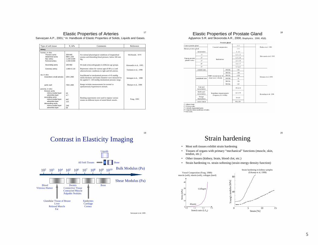
Elastic Properties of ArteriesSarvazyan A.P., 2001,” In: Handbook of Elastic Properties of Solids, Liquids and Gases.

18Elastic Properties of Prostate GlandAglyamov S.R. and Skovoroda A.R., 2000, Biophysics, 2000, 45(6).

19

Contrast in Elasticity Imaging

102 105104103 106 107 108 109 1010

Shear Modulus (Pa)Bone

All Soft Tissues

EpidermisCartilageCornea

DermisConnective TissueContracted MusclePalpable Nodules

Glandular Tissue of BreastLiver

Relaxed MuscleFat

Bone

Liquids

Bulk Modulus (Pa)

BloodVitreous Humor


20

Strain hardening

Elastin

Collagen

Stretch ratio (L/L0)1.0 1.1 1.2 1.3

0

10

20

40

30

Stre

ss(k

Pa)

Vessel Composition (Fung, 1988):muscle (soft), elastin (soft), collagen (hard)

Strain hardening in kidney samples(Erkamp et al, 1998)

0 5 10 15

40

80

Strain [%]

You

ng's

mod

ulus

[kPa

]

• Most soft tissues exhibit strain hardening

• Tissues of organs with primary “ mechanical” functions (muscle, skin,tendon, etc.)

• Other tissues (kidney, brain, blood clot, etc.)

• Strain hardening vs. strain softening (strain energy density function)

6

21

Wellman et al., 1999

Strain hardening22

Strain hardening

Krouskop et al, 1998Ophir et al., 2001

This and other graphs as well as other literaturedata suggest that tissuestrain hardening (or nonlinearity in stress-strain relations) can be used for

tissue analysis including composition, differentiation, etc.

23

Anisotropy• Arterial wall: orthotropic material – 9 constants

two orthogonal planes of symmetry• Muscle: transversely isotropic – 5 constants

axis of symmetry• Isotropic – 2 constants

0 5 10 15 200

4

8

12

16

Strain (% )

Str

ess(

kPa)

Alongfibers

Acrossfibers

24

Viscosity

Time

Constant Deformation

Stress RelaxationStre

ssD

efor

mat

ion

Time

Def

orm

atio

nL

oad Constant Load

Creep

Creep Stress Relaxation

• Shear viscosity: shear waves

• Bulk viscosity: longitudinal ultrasound waves

• Viscoelastic models:Maxwell, Voigt, Kelvin, KVFD, etc.

• Is there a characteristic time?

0 30 60 90

4

8

12

Time(min)

Forc

e(N

)

Cornea

7

25

ViscosityS

tres

s

Strain

Loading Cycles

Elongation

Load

1st cycle

5th

>10th cycle

• Hysteresis loops:independent of the rate of loading (most soft tissues)

• Pseudoelastic material:elastic after preconditioning (with hysteresis)

26

Mechanical Properties of Tissue:References

• Duck, F.A. Physical properties of tissues. Academic press; New York, 1990

• Fung YC. Biomechanics – mechanical properties of living tissues. Springer-Verlag; New York, 1981

• Krouskop TA, Wheeler TM, Kallel F, Garra BS, Hall TJ, “The elastic moduliof breast and prostate tissues under compression,” Ultrasonic Imaging vol. 20pp. 260-274, 1998

• Aglyamov SR, Skovoroda AR, “Mechanical properties of soft biologicaltissues,” Biophysics, Pergamon, 45(6):1103-1111, 2000.

• Sarvazyan AP, “Elastic properties of soft tissues,” In: Handbook of ElasticProperties of Solids, Liquids and Gases, Volume III, Chapter 5, 107-127, eds.Levy, Bass and Stern, Academic Press, 2001

• Other text books and archival publications

27

Phantoms for Elasticity Imaging• Tissue-mimicking phantoms

– Gelatin gels

– Agar-agar and gelatin mixtures

– Rubber (plastisol, silicone)materials

– PVA (poly-vinyl alcohol)

– Polyacrilamyde gels

• Tissue-containing phantoms

– Gelatin gels

– Agar-agar and gelatin gels

– Polyacrilamyde gels

Hall et al., 1997Other papers

• Gelatin and Gelatin/Agar-agar

– Easy to prepare

– E ~ Cn, C – concentration, n=[1-2]

– Short shelf life

– Additives are possible

• Plastisol

– Time-stable phantoms

– Requires excessive heating duringpreparation

• PVA

– Freeze-thaw cycles to varyelasticity

– Time-stable

28

• PVA (poly-vinyl alcohol) tissue-mimicking phantom

• Background:8% PVA solution1% silica (40µm diameter)1 freeze/thaw cycle

• Inclusion:10% PVA solution2% silica particles3 freeze/thaw cycles

• Imaging:SONIX RP imaging system(Ultrasonix, Inc.)5-7 MHz, 40 mm linear probe

• Deformationsmanual0.3%

Phantoms for Elasticity Imaging: Preparation

Park et al., 2007

50mm

50mm

50mm

10mm

8

29

Phantoms for Elasticity Imaging:References

• Madsen EL, Frank GR, Krouskop TA, Varghese T, Kallel F, Ophir J,“Tissue-mimicking oil-in-gelatin dispersions for use in heterogeneouselastography phantoms,” Ultrasonic Imaging vol. 25 pp. 17-38, 2003

• Madsen EL, Hobson MA, Frank GR, Shi H, Jiang J, Hall TJ, Varghese T,Doyley MM, Weaver JB, “ Anthropomorphic breast phantoms for testingelastography systems,” Ultrasound Med Biol. vol. 32 pp. 857-874, 2006

• Hall TJ, Bilgen M, Insana MF, Krouskop TA, “Phantom materials forelastography,” IEEE Trans. UFFC, vol. 44 pp. 1355-1365, 1997

• Surry KJM, Austin HJB, Fenster A, Peters TM, “Poly(vinly alcohol) cryogelphantoms for use in ultrasound and MR imaging,” Phys. Med. Biol., vol. 49pp. 5529-5546, 2004


• Where to buyATS Laboratories, Inc. (http://www.atslabs.com/)

30

Elasticity Imaging using ...?

Computerized Tomography:spatial distribution of the absorption (density)

MRI:proton spin density and relaxation time constants

Ultrasound Imaging:variation in acoustical impedance(bulk modulus and density)

Optical Imaging:refraction index

31

Elasticity Imaging – Approaches

Static (strain-based, or reconstructive)imaging internal motion under static deformation

Dynamic (wave-based)imaging shear wave propagation

Mechanical (stress-based, also reconstructive)measuring tissue response at the surface

32

How … Static Elasticity Imaging?

Har

d

Sof

t

Displacement Strain

Ra

nge

9

33

How … Static Elasticity Imaging?

• Capture data during deformation

• Estimate displacements

• Compute strain tensor

• Reconstruct mechanical properties

34

Elasticity Imaging – Main Components

• Capture data duringexternally or internally applied

tissue motion or deformation

• Evaluate tissue response(displacement, strain, stress)

• Reconstruct elastic modulus based ontheory of elasticity

Theory of elasticity is common part inall approaches in Elasticity Imaging

35

• Strain

• Stress

• Constitutive relationships

• Equations of equilibrium

Theory of Elasticity(Static Approach)

011

0

L L

Lε −=

L0

L=L0+∆L

FF

S

S0

∂∂

∂∂+

∂∂

+∂∂=

j

k

i

k

i

j

j

iij x

u

x

u

x

u

x

u

2

1ε

11

F

Sσ =

1111 εσ E= E – Young’s modulus ijijiiij µεδλεσ 2+=

333231

232221

131211

εεεεεεεεε

333231

232221

131211

σσσσσσσσσ

11

1

0x

σ∂ =∂

0=+∂∂

∑ ii j

ij fx

σ

General (3-D) case

36

Equations of Equilibrium

0)2())(())(())((

0))(()2())(())((

0))(())(()2())((

33

3

33

2

2

3

23

1

1

3

13

3

2

2

1

1

3

22

3

3

2

32

2

22

1

1

2

13

3

2

2

1

1

2

11

3

3

1

31

2

2

1

21

1

13

3

2

2

1

1

1

=+∂∂

∂∂+

∂∂+

∂∂

∂∂+

∂∂+

∂∂

∂∂+

∂∂+

∂∂+

∂∂

∂∂

=+∂∂+

∂∂

∂∂+

∂∂

∂∂+

∂∂+

∂∂

∂∂+

∂∂+

∂∂+

∂∂

∂∂

=+∂∂+

∂∂

∂∂+

∂∂+

∂∂

∂∂+

∂∂

∂∂+

∂∂+

∂∂+

∂∂

∂∂

fx

u

xx

u

x

u

xx

u

x

u

xx

u

x

u

x

u

x

fx

u

x

u

xx

u

xx

u

x

u

xx

u

x

u

x

u

x

fx

u

x

u

xx

u

x

u

xx

u

xx

u

x

u

x

u

x

µµµλ

µµµλ

µµµλ

Examples (incompressible material)

Small deformations of linear, isotropic (i.e., Hookean) material

F1

x1

x2

x3

01 3µε=FSemi-infinite elastic medium

Rigidcircular

dieF

R

W

µRWF 8=

10

37

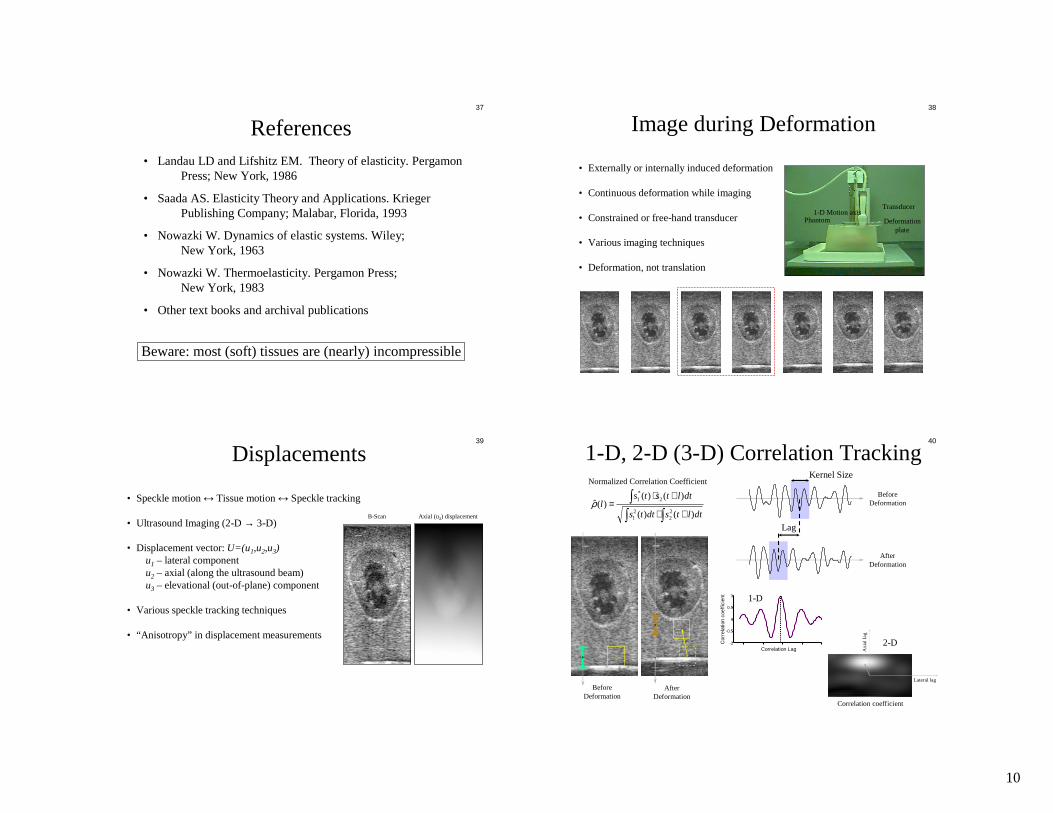
References• Landau LD and Lifshitz EM. Theory of elasticity. Pergamon

Press; New York, 1986

• Saada AS. Elasticity Theory and Applications. KriegerPublishing Company; Malabar, Florida, 1993

• Nowazki W. Dynamics of elastic systems. Wiley;New York, 1963

• Nowazki W. Thermoelasticity. Pergamon Press;New York, 1983


Beware: most (soft) tissues are (nearly) incompressible

38

Image during Deformation

Transducer

Phantom1-D Motion axis

Deformationplate

• Externally or internally induced deformation

• Continuous deformation while imaging

• Constrained or free-hand transducer

• Various imaging techniques

• Deformation, not translation

39

Displacements

B-Scan Axial (u2) displacement

• Speckle motion↔ Tissue motion↔ Speckle tracking

• Ultrasound Imaging (2-D → 3-D)

• Displacement vector: U=(u1,u2,u3)u1 – lateral componentu2 – axial (along the ultrasound beam)u3 – elevational (out-of-plane) component

• Various speckle tracking techniques

• “Anisotropy” in displacement measurements

40

1-D, 2-D (3-D) Correlation Tracking

AfterDeformation

Kernel Size

Lag

BeforeDeformation

AfterDeformation

BeforeDeformation

Correlation Lag

-0.5

-1

0

0.5

1

Cor

rela

tion

coef

ficie

nt

Lateral lag

Axi

alla

g

Correlation coefficient

Normalized Correlation Coefficient

1-D

2-D

∫∫∫

+⋅

+⋅=

dtltsdtts

dtltstsl

)()(

)()()(ˆ

22

21

2*1ρ

11

41

Strains• Displacement vector → Strain tensor

• Displacement derivatives

• Six (3-D) or three (2-D)independent components

• Sources of error

• Improvement and Optimization

• Effect of strain hardening, anisotropy, etc.

Axial (u2) displacement Normal axial (ε22) strain

∂∂

∂∂+

∂∂

+∂∂=

j

k

i

k

i

j

j

iij x

u

x

u

x

u

x

u

2

1ε

333231

232221

131211

εεεεεεεεε

42

Static or ReconstructiveUltrasound Elasticity Imaging

B-Scan

Deform and image

Displacements

Track internal motion

Strains

Evaluate deformations

Elasticity

ReconstructYoung’s or shearelastic modulus

43

Deformation vs. rotation and translationtranslation – no information about tissue elasticityrotation – no information about tissue elasticity and speckle tracking difficultiesdeformation – consider “ anisotropy” in displacement measurements (example 1)

Volumetric deformation vs. 1-D or 2-D US imagingdeformation – control the deformation state (i.e., plane strain) if possible

Deformation vs. temporal and spatial samplingcontrol deformation rate and/or frame rate and spatial sampling

Deformation vs. distribution and symmetries of elasticityspatial symmetries (if any) must be considered to assist

displacement estimationimaging of strain and interpretation (example 1 and 2)elasticity reconstruction (example 1 and 2)

Deformation: Challenges44

Strain Imaging: ChallengesSources of error in strain images

ultrasound imaging system (electronic SNR, etc.)interpolationstrain induced decorrelationother sources (out-of-plane motion, peak hopping, etc.)

Optimal SNR and CNR in strain imagesshort-time correlation, companding, temporal stretching, strain filter, etc.adaptive strain imaging for large deformations, multi-compression, etc.

Anisotropy in displacement measurementsincompressibility processingother approaches (phase sensitive interpolation, grid slopes, etc.)

Effect of tissue strain hardening on strain imagesutilize as independent parameter of tissue differentiation

12

45

Correlation Lag

-0.5

-1

0

0.5

1C

orre

latio

ncoe

ffici

en

t

Truedisplacement

False PeakJitter

A fundamental limit on delay estimation

Walker and Trahey, 1995

( )

−

+

+≥ 1

11

1

122

32

223230 SNRBBTf ρπ

στ

SNR – root mean squared signal-to-noise ratioρ – correlation coefficientστ – root mean squared time delay estimate error

f0 – center frequencyT – the observation timeB – fractional bandwidth

time↔ distance(via sound velocity)

46

Walker and Trahey, 1995

A fundamental limit on delay estimation

47

Cor

rela

tion

Coe

ffic

ient

Correlation Lag

-0.5

-1

0

0.5

1 RFComplex

0

Cor

rela

tion

Phas

e

BasebandAnalytic

ππππ

π/2π/2π/2π/2

−−−−π/2π/2π/2π/2

−−−−ππππCorrelation Lag

Interpolation Error

O’Donnell et al, 1993Lubinski et al, 1999

Some other approaches are discussed in:Cespedes et al, 1995Cohn et al, 1997Pesavento et al, 1999Geiman et al, 2000

Two-step approach(computationally efficient)

• Correlation peak position ofcomplex baseband signal

• Phase zero-crossing ofanalytic signal correlation

48

Strain Decorrelation

No strainDisplacement error ~ 1 / Kernel Size(Kernel size↔ Observation time ↔Window size)

Strain decorrelationReduce kernel size

Filter correlation functionsSpatial resolution vs. error

Strain � Decorrelation � Displacement Error � Strain Error

T = 1.3 µsec

T = 0.35 µsec (with filter)True strain

40 50 600

1

2

3

4

Time (µsec)

Stra

in(%

)

ρF(t0, t0 +τ)^

τ

tρ(t0, t0 +τ)^

ρ(t0+ ξ1 , t0 + ξ1 +τ)^

ρ(t0- ξ1 , t0 - ξ1 +τ)^

h(t)

Filtered CorrelationCoefficient FunctionCorrelation Filter

Correlation CoefficientFunctions

Σ

t

τ

ττ h(-ξ1)

h(+ξ1)h(0)

Lubinski et al, 1999

13

49

Time Delay Estimation andInterpolation Techniques

Time Delay EstimationDoppler-based techniquesOptical FlowNormalized CovarianceNormalized Cross-correlationHybrid-sign CorrelationPolarity-coincidence CorrelationCross-correlationSum of Squared Differences (SSD)Sum of Absolute Differences (SAD)Mutual InformationMany, many other algorithms

Lubinski et al, 1999

InterpolationParabolicPhase zero crossingCosineSplineGrid slopesAutocorrelation

50Kernel size vs. resolution and SNR

Liu et al., 2003

Resolution

Kernel 0.86 mm

Kernel 0.43 mm

SNR

Formula for optimal kernel size:B – bandwidths – strainf0 – center frequency

Varghese et al., 1998

• Correlation window is longer than pulse length:the axial resolution of elasticity imaging isdetermined by the correlation window.

• Correlation window decreases to pulse length andbelow: spatial resolution is ultimately limited bythe bandwidth of the ultrasonic imaging system.

51

Elasticity Imaging – Approaches

Static (strain-based, or reconstructive)imaging internal motion under static deformation

Dynamic (wave-based)imaging shear wave propagation

Mechanical (stress-based, also reconstructive)measuring tissue response at the surface

52

• Strain

• Stress

• Constitutive relationships

• Equations of motion

Theory of Elasticity(Dynamic Approach)

011

0

L L

Lε −=

L0

L=L0+∆L

FF

S

S0

∂∂

∂∂+

∂∂

+∂∂=

j

k

i

k

i

j

j

iij x

u

x

u

x

u

x

u

2

1ε

11

F

Sσ =

1111 εσ E= E – Young’s modulus

333231

232221

131211

εεεεεεεεε

333231

232221

131211

σσσσσσσσσ

211 1

21

u

x t

σ ρ∂ ∂=∂ ∂

General (3-D) case

2

2

i j ii

i j

uf

x t

σρ

∂ ∂+ =∂ ∂∑

22i j i i i ji jii

i ji j t t

εεξ δσ λ δ ηε µε= +∂∂ ++

∂ ∂

14

53

Example: plane waves• Infinite homogeneous (λ,µ=const) elastic medium (i.e., ignore bulk and shear

viscosities), no body forces (fi=0)

• Assume that u1=u1(x1,t), u2=u2(x1,t), and u3=u3(x1,t)

23

2

3

3

33

2

2

3

23

1

1

3

13

3

2

2

1

1

3

22

2

2

3

3

2

32

2

22

1

1

2

13

3

2

2

1

1

2

21

2

1

3

3

1

31

2

2

1

21

1

13

3

2

2

1

1

1

)2())(())(())((

))(()2())(())((

))(())(()2())((

t

u

x

u

xx

u

x

u

xx

u

x

u

xx

u

x

u

x

u

x

t

u

x

u

x

u

xx

u

xx

u

x

u

xx

u

x

u

x

u

x

t

u

x

u

x

u

xx

u

x

u

xx

u

xx

u

x

u

x

u

x

∂∂=

∂∂

∂∂+

∂∂+

∂∂

∂∂+

∂∂+

∂∂

∂∂+

∂∂+

∂∂+

∂∂

∂∂

∂∂=

∂∂+

∂∂

∂∂+

∂∂

∂∂+

∂∂+

∂∂

∂∂+

∂∂+

∂∂+

∂∂

∂∂

∂∂=

∂∂+

∂∂

∂∂+

∂∂+

∂∂

∂∂+

∂∂

∂∂+

∂∂+

∂∂+

∂∂

∂∂

ρµµµλ

ρµµµλ

ρµµµλ

( )ρ

µλρµλ 2cwhere0

102 l2

12

221

12

21

2

21

12 +==

∂∂−

∂∂→=

∂∂−

∂∂+

t

u

cx

u

t

u

x

u

l

ρµρµ ==

∂∂

−∂

∂→=

∂∂

−∂

∂t2

)3(22

221

)3(22

2

)3(22

21

)3(22

cwhere01

0t

u

cx

u

t

u

x

u

t

Longitudinal wave(ultrasound)

Shear wave

54

Catheline, Fink et al. 1999Laboratoire Ondes et Acoustique, Francehttp://www.loa.espci.fr/

Transient ElastographyThe displacement vector is not always orthogonal to the propagation vector:

finite medium, finite size vibratorshear wave is not purely transverse

Transmit low frequency shear wavesmechanical vibration parallel to ultrasound beam

x

z

y

Imagearea

55

Transient ElastographyImage shear waves and measure its velocity using ultrafast imaging and motion tracking

Activeelements

Transmitbeamprofile

Transmitwave front

75m

m

250 beams

Time needed to acquire 1 frame:

lbeam c

Rt

⋅≥ 2

ms25256mm/µm5.1

mm752# ≈⋅⋅=⋅= beamstt beamframe

ConventionalImaging

UltrafastImaging

µs100mm/µm5.1

mm752 ≈⋅== beamframe tt

56

Transient ElastographyEvaluate shear modulus from shear wave velocity

Isotropic, homogeneous, elastic medium

Shear wave propagation equation

Local inversion algorithm

( ) ( ) uut

u rrrrrr

∆+∇∇+=∂∂ µµλρ .

2

2

shearcompression

zy,x,i,2

2

=∆=∂∂

ii u

t

u µρ

( ) ( ) ( ) ( )∑=

−

∂

∂+∂

∂∂

∂=N

ns z

tzxu

x

tzxu

t

tzxu

NzxV

1

1

2

2

2

2

2

2 ,,,,,,1,

15

57

Transient Elastography

-20 0

10

20

30

40

5020

Ultrasound Image

1

2

3

4

5

10

20

30

40

50

-20 0 20

Shear velocity map

m/sBercoff et al. 2003

58

Acoustic Radiation Force Imaging

Nightingale, Trahey et al.Duke University

Dire

ctio

nof

Wav

eP

ropa

gatio

n

1. Focused Acoustic RadiationForce generates localized,impulsive (<0.1 ms) tissueexcitation

2. Track tissue response withsame ultrasonic transducer usedfor force generation

3. Repeat in multiple locationsthroughout 2D FOV

4. Generate images of relativetissue response within theregion of excitation(displacement after forceremoval, recovery time, etc) toassess structural informationabout tissue

RadiationForce

c

IF taα2=

Transducer

59

Bercoff et al. 2004

Shear WaveImaging

60

Bercoff et al. 2004

SupersonicShear Wave Imaging

16

61

Elasticity Imaging Systems(Static / Dynamic)

• Siemens/Acuson Antares

• Hitachi Imaging System

• Sonic RP by UltrasonixMedical, Inc.

• Volcano Therapeutics IVUSImaging

• Winprobe Research Platform

• Other systems

• Supersonic Imaging, Inc.

• Siemens

• Echosens

• Other systems

62

Siemens Sonoline Elegra and Acuson Antares systems

eSie Touch elasticity imaging• Provides additional qualitative information bydemonstrating the typical internal characteristicspattern of three cysts.

eSie Touch elasticity imaging• Improves border delineation of this biopsy-proveninvasive ductal carcinoma. Live dual imagingprovides real time comparison of elastogram tostandard 2D imaging.

www.siemens.com

63

Hall et al, 2006www.engr.wisc.edu/bme/faculty/hall_timothy.htmlwww.medphysics.wisc.edu/medphys_docs/people/hall/hall.html

Fibroadenoma:changing contrastequal lesion size ratio

IDC:constant contrastlarge lesion size ratio

64

Hall, Zhu et al, 2003

17

65

Regner et al. 2006

Lesion size comparison technique

Benign fibroadenoma

WR - size ratios for widthAR - size ratios for area

A, B, C, D, E – five observers

66

Regner et al. 2006

Lesion size comparison techniqueInvasive ductal carcinoma



67

Regner et al. 2006


Benign fat necrosis



Potential problems: for some lesions it is difficult to distinguish from thesurrounding breast tissue on B-mode images.

68

Regner et al. 2006


18

69Hitachi HI Vision 8500/900systems

Nonscirrhous type invasive ductal carcinoma in 29-year-oldwoman

Fibroadenoma with in 39-year-old woman

Itoh et al. 2006

70

Nightingale, Trahey et al.

ARFI image of an in-vivo breast lesion (an infected lymph node) showing differences in displacementand recovery response of different tissues to radiation force excitation

Acoustic Radiation Force Imaging:Breast

In vivo Breast Lymph Node (Reactive, Benign)

Lateral Position (mm)

Dep

th(m

m)

B-mode Max. Disp. (~5µm)

Typical Lymph Node Histology

Reproduced from Wheater’s FunctionalHistology, 4th Ed.

Nightingale et al.; Trahey et al.Duke University

In Vivo Breast LesionsIDAC

B-modeARFI Displacement

(~6.5 µm)

Fibroadenoma

B-modeARFI Displacement

(~1.8 µm)

IDAC Fat Necrosis

Lateral Position (mm) Lateral Position (mm)

Lateral Position (mm)Lateral Position (mm)

B-modeCombined

ARFI ImageB-mode

ARFI Displacement(~5.1 µm)

Nightingale et al.; Trahey et al.

19

73Supersonic Imagine:Elasticity Imaging of Breast

74

Gray-scale transrectalultrasonography

T2-weighted image Dynamic contrast-enhanced image

Color Doppler ultrasonography

Histopathology

Sumura et al., 2007

Elasticity Imaging of Prostate cancerReal-time

elastography

75

Ruhr Center of Competence for Medical EngineeringBochum, Germany (http://www.hf.ruhr-uni-bochum.de)

Real-time (30 fps) Strain Imaging of Prostate:Digital System, 7.5 MHz

76

Varghese et al. 2002

Elastography of Thermal Lesions in the Liverafter RF Ablation

20

77Monitoring liver stiffness after RF ablation

Bharat et al., 2005

normal liverliver with a lesionafter RF ablation

Canine liver tissue in vitro

Ex Vivo RF Liver AblationBefore RF Ablation After RF Ablation


Staging of Liver Fibrosis with Radiation Force


Key clinical question is degree to which liver fibrosis has occurredBiopsy? Imaging?

Quantitative measure of liver stiffness is neededSWEI: new shear wave speed estimation approach

eliminates 2nd order differentiation

80

Fibroscan

http://www.echosens.com

21

81

Non-invasive staging of liver fibrosis

Friedrich-Rust et al. 2007

A. Real-time elastography; B. Aspartate transaminase-to-platelet ratio index; C. Elasticity- laboratory combination values

82

SuperSonic Imagine:

ShearWave Elastography

Deffieux at al. 2007

In vivo assessment of Young’s modulus in a healthy volunteer

83

Ulrasonix Sonix RPImaging System

www.ultrasonix.com

84

Winprobe Elasticity Imaging System(FPGA-based solution)

www.winprobe.com

-1%

-2%

-1%

-2%

22

85

Characterizing lesions - Palpograms

Cespedes, De Korte et al./Ultrasound in Med. & Biol., Vol. 26, No. 3, pp. 385–396, 2000

86

de Korte, Mastik and van der SteenErasmus Medical Center, Rotterdamhttp://www.eur.nl/fgg/thorax/elasto/

0 20 40 60 80 100 12040

60

80

100

120

140

Frame no.

Intr

a-co

rona

rypr

ess

ure

[mm

Hg]

In vivo acquisition scheme

Strain [%]

1.0

0.0

Eur Heart J 23(5): 405-413 (2002)

87

de Korte, Mastik and van der SteenErasmus Medical Center, Rotterdamhttp://www.eur.nl/fgg/thorax/elasto/

3 Dimensional Elastography:feasibility in a human coronary

88

Vascular Strain Imaging usingArterial Pressure Equalization

Kim et al, Weitzel et alUniversity of Michiganhttp://bul.eecs.umich.edu/

MAP

Strain(%)

Pres

sure

(m

mH

g)40

80

120 } Pulse Pressure

}

23

89

Vascular Strain Imaging usingArterial Pressure Equalization

Kim et al, Weitzel et alUniversity of Michiganhttp://bul.eecs.umich.edu/

90Clinical Data: 5 healthy, 5 diseased arteries

Kim et al, Weitzel et al

healthy diseased

6

12

0

Stra

in (

%)

Stra

in (

%)

30

60

0

healthy diseased

Stra

in R

ate

(Hz)

0.5

1.5

0

1.0

Stra

in R

ate

(Hz)

4

8

0

Phy

siol

ogic

Pre

ssur

eP

ress

ure

Equ

aliz

atio

n

91

CardiacStrain and Strain Rate

Imaging

• Cross-correlation methodhigh sensitivityhigh accuracy2-D or 2.5-Dcomputationally intensive

• Gradient velocity methodfast1-D (axial)aliasing

• Real-time implementation isrequired

D’hooge et al. 2000

92

Different parametric imaging in 3-/4D display, all from a normal subject. Left to right: The red-blue display of tissue velocity, the colored bands of tissuetracking and the yellow-blue display of strain rate. In tissue velocity, lighter color represents higher velocities, showing clearly the velocity gradient from base toapex both in systole and diastole. In tissue tracking, each color represents an interval of 2 mm displacement, as shown by the legend. This means that redrepresents 2 – 4 mm displacement, increasing to magenta showing >14 mm at the base. Strain rate shows shortening in yellow to red, lengthening in blue, darkercolor represents more deformation. Some inhomogeneity is visible due to noise and dropouts. Top to bottom: Bull's eye display both in systole and diastole (excepttissue tracking), M-mode array from all six walls with apex on top and base at the bottom with ECG and a 3D surface reconstruction, velocity and strain rate insystole and diastole. The bull's eye projection shows all of the surface, but the area is distorted; the apex is progressively diminished, while the base is over-represented, the 3D figure shows a representation of the true area, but has to be rotated to see all of the surface. Reconstruction is done from three separate cine-loops, synchronized by means of ECG. The ECG at the left is inverted, but is from the same patient, as may be seen by the end of the cycle, where there is noise inthe ECG signal. The aortic annulus and location of the imaging planes are added for orientation. Støylen, 2003

Cardiac Strain and Strain Rate Imaging

24

93

Deep Vein Thrombosis (DVT) andPulmonary Embolism (PE)

94

Softer ↔ Harder-0.10-0.55

Triplex Ultrasound: Grayscale, Doppler, Elasticity

•• SpragueSprague--DawleyDawley rats (300 g)rats (300 g)

•• Surgically induced clots in IVCSurgically induced clots in IVC

•• Imaging studies clots atImaging studies clots at22--day (acute)day (acute)66--day (subday (sub--acute)acute)99--day (chronic)day (chronic)

•• SiemensSiemens SonolineSonoline ElegraElegra99--13 MHz center frequency13 MHz center frequency

•• 22--D correlation and strain imagingD correlation and strain imaging

Emelianov, Rubin et al, 2000 and 2002

95

Xie et al 2004

Nor

mal

ized

Str

ain

Age (day)2 4 6 8 10 12

0

0.5

1

1.5

2

2.5First Set of Experiments

(learning set, 10 rats)

Second Set of Experiments(4 rats)

• Fitting of data from the first set ofexperiments

ε=e(aD+b)

ε – normalized strainD – age of the clot (day)

• Can first data set predict the age of theclot in the second set of experiments ?

Can elasticityimaging age

DVT ?

True age (day)

Estim

ated

age

(da

y)

2 4 6 8 10 122

4

6

8

10

12

Estimation error:± 0.8 day

96

Elasticity Imaging to Age DVT

Rubin et al., 2006

-60 % -6 %

11m

m

17 mm

Chronic DVT

22m

m

-20 % 0 %

Acute DVT

Strain magnitude Ultrasound backscatter

25

97

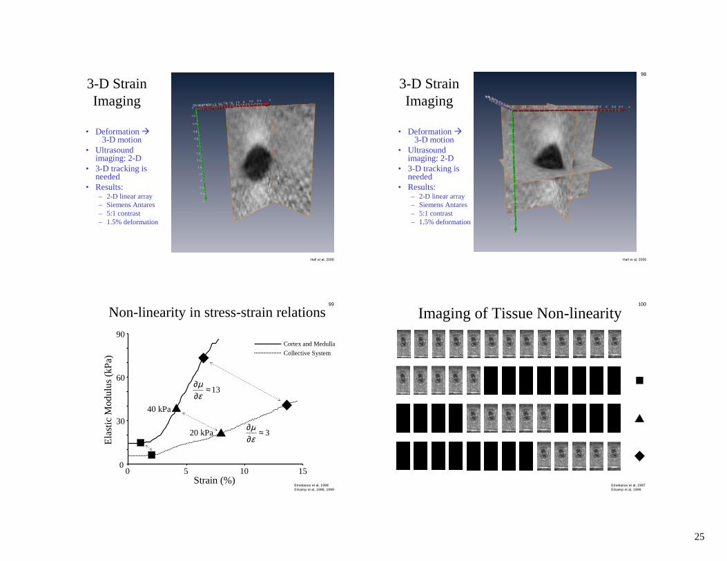
3-D StrainImaging

Hall et al, 2006

• Deformation �3-D motion

• Ultrasoundimaging: 2-D

• 3-D tracking isneeded

• Results:– 2-D linear array– Siemens Antares– 5:1 contrast– 1.5% deformation

98

3-D StrainImaging

Hall et al, 2006

• Deformation �3-D motion

• Ultrasoundimaging: 2-D

• 3-D tracking isneeded

• Results:– 2-D linear array– Siemens Antares– 5:1 contrast– 1.5% deformation

99

0 5 10 150

30

60

90

Strain (%)

Ela

stic

Mod

ulus

( kP

a)

Cortex and Medulla

Collective System

Non-linearity in stress-strain relations

13≈∂∂εµ

3≈∂∂εµ

40 kPa

20 kPa

Emelianov et al, 1998Erkamp et al, 1998, 1999

100

Imaging of Tissue Non-linearity

Emelianov et al, 1997Erkamp et al, 1999

26

101

0 10 20 300

1

2

3

4

5

6

Strain(%)

You

ng’s

Mod

ulus

(E/E

0)

0 4 8 120

10

20

30

40

50

60

Strain (%)

You

ng’s

Mod

ulus

(kP

a)Remote (i.e., Elasticity Imaging) Direct (i.e., tissue sample)

Emelianov et al, 1997; Erkamp et al, 1998

102

ViscoelasticityImaging

Strain ↔ Elasticity Creep ↔ Viscosity

103

T1(x)

s tra

in

time

strain image sequence

)))(/exp(1()()(),( 110 xxxx Ttktk ∆−−×+=∆ εεε

x

)(0 xε)()( 10 xx εε +

0 t∆ t∆2 tN∆

Retardance Time Imaging, T1

Gelatin phantomwith inclusionhaving twice thecollagen density

Michael F. Insana et al. University of Illinoisat Urbana-Champaignhttp://ultrasonics.bioen.uiuc.edu

104

In Vivo Patient Studies

Fib

road

enom

a

3

4

5

6

7

820

40

60

80

100

T1:1

-2

0

2

4

6

8

10(sec)10mm T1StrainSonogram

T1:4

0

0

00

2

4

6

8

10

4

6

8

20

40

60

T1StrainSonogram10mm

(sec)

IDC

Two patients with 1-cm, non-palpable lesions detected mammographically. With theretardance time image, malignant and benign lesions can be differentiated because ofdifferences in the collagen ultrastructure between the two lesion types.

Sridhar M, Liu J, Insana MF, “ Elasticity imaging of polymeric media,” ASME J Biomechan Eng (in press)Insana MF, Pellot-Barakat C, Sridhar M, Lindfors K, “ Viscoelastic imaging of breast tumor microenvironment with ultrasound,”

J Mammary Gland Biol Neoplasia. 9: 393-404, 2004Insana MF, “ Elasticity imaging,” In: Wiley Encyclopedia of Biomedical Engineering, M Akay, ed., ISBN: 0-471-24967-X, Hoboken: John

Wiley & Sons, Inc., 2006

27

105

Acknowledgements

All who contributed to

the field of Elasticity Imaging and

to this presentation

Documents

Ultrasound Elasticity Imaging · Young ’s Modulus ( kPa ) Ductal fibroadenoma Infiltrative ductal cancer with fibrous tissue predominating. Fibroadenomas of glandular origin Infiltrative