Uncertainties in the Resistance Prediction of Underwater ... Meeting Proceedings/RTO... · Uncertainties in the Resistance Prediction of Underwater Vehicles ... Uncertainties in the

RTO-MP-AVT-147 58 - 1

Uncertainties in the Resistance Prediction of Underwater Vehicles

Joseph J. Gorski, Michael P. Ebert and Lawrence P. Mulvihill Naval Surface Warfare Center, Carderock Division

9500 MacArthur Boulevard West Bethesda, MD, 20817-5700, USA

[email protected]; [email protected]; [email protected]

ABSTRACT

The current effort demonstrates that accurate resistance predictions can be obtained using unstructured grids for solving the Reynolds Averages Navier-Stokes (RANS) equations, as compared to experimental data, for several unappended bodies of revolution with varying Reynolds numbers and length/diameter ratios including: 5, 8, 10 and 11. This was demonstrated for a variety of turbulence models and grids. Comparisons with skin friction, boundary layer, and resistance coefficients also demonstrates that just as accurate results could be achieved with unstructured grids as with structured grids. Issues associated with the prism layers needed for accurate predictions of the boundary layers, with unstructured grids, are also discussed. Uncertainty estimates were not obtained with the unstructured grids due to the complications associated with them and lack of an accepted method of performing an uncertainty analysis with them. However, results shown here for an unstructured code with structured grids also show that just as high accuracy and low levels of uncertainty can be obtained with an unstructured code as a structured .

1.0 INTRODUCTION

Resistance estimation is an important part of design for many types of vehicles. For marine vehicles the drag generated by a particular configuration is a dominant driver of the powering requirements of that configuration. The thrust of the propulsor must match the drag of the vehicle, including all appendages, for self propulsion. In fact, for early stage design resistance and powering are often the only hydrodynamic aspects considered in a ship design process and maneuvering and seakeeping aspects are determined after the basic design has been established.

Before 1874, ship performance was largely based on full-scale experience. It was then that Froude[1] had the insight to split ship resistance into wave making and frictional components and to treat these components independently. Wave making or pressure resistance was assumed to scale with the Froude number and frictional resistance scaled with the Reynolds number. Model scale ship tests can often be performed at the same Froude number as full scale ships, but not at the same Reynolds number. However, it was assumed that the frictional component of resistance could be estimated by the drag of a flat plat with an equivalent wetted surface area and this information could be used to obtain the full scale resistance of a ship. The assumptions themselves provide an excellent way to make the full scale resistance prediction manageable, but the approach is not without problems. A well established curve for estimating flat plate frictional resistance was not accepted before the efforts of Schoenherr [2] and the International Towing Tank Conference (ITTC) recommended a different line at their 1957 Conference [3]. The acceptance of the ITTC 1957 line was not

Gorski, J.J.; Ebert, M.P.; Mulvihill, L.P. (2007) Uncertainties in the Resistance Prediction of Underwater Vehicles. In Computational Uncertainty in Military Vehicle Design (pp. 58-1 – 58-18). Meeting Proceedings RTO-MP-AVT-147, Paper 58. Neuilly-sur-Seine, France: RTO. Available from: http://www.rto.nato.int.

UNCLASSIFIED/UNLIMITED


http://www.rto.nato.int/

mailto:[email protected]




58 - 2 RTO-MP-AVT-147

without considerable debate and was accepted at the 1957 conference only on an interim basis. The main reason it was accepted then was because it provided a convenient mathematical formulation for estimating the resistance as opposed to a highly accurate estimation of it. Various organizations have never accepted the ITTC formula and some still use the Schoenherr formula today. It was also recognized early that there can be dependence on the frictional resistance due to the shape, or form, of the geometry and a simple flat plate frictional estimate would be inadequate due to pressure gradient and surface curvature effects. In fact, the ITTC 1957 line contains an added component for form factor, on the order of 12% over the Schoenherr formula, at low Reynolds numbers. This is because the Schoenherr formula was based on flat plate data, but the ITTC 1957 line was based on a number of model scale data sets for relevant hull forms at that time. Today, many organizations using the Schoenherr or ITTC 1957 line for their estimations have an additional form factor built in based on experience and the particular hull form. Obtaining the pressure resistance is also problematic so when estimating full scale resistance, and subsequent powering, tow tank facilities add an extra correlation allowance to account for deficiencies in the modelling and anything else that might be going on at full scale. The correlation allowance can only be obtained after the ship has been built and evaluated at full scale. Despite these problems the approach has stood the test of time as variations of this method are still widely used today by many shipyards and testing facilities. When new or different hull forms are evaluated is when serious deficiencies in the procedure can be discovered and new approaches need to be considered.

The computer advances in the last decade have been a significant catalyst for improving our ability to predict fluid flow. The increased computer power has led to Reynolds Averaged Navier-Stokes (RANS) calculations becoming more routine. In 1996 ITTC [4] concluded that RANS codes had matured enough to be integrated into the design process for addressing issues associated with resistance and propulsion. RANS codes are being used in marine design by a variety of organizations including military applications, as demonstrated by Gorski and Coleman [5] for a submarine sail and by Gorski et al [6] for a naval combatant, where design decisions were based on the predicted resistance and flow field.

Despite the success of RANS computations, and the inherent limitations of the simpler Froude hypothesis for ship resistance, one could argue the simpler Froude approach is still more widely accepted and used than RANS. Some of it is obviously the longer time associated with getting solutions from RANS analysis. Some of it is also the lack of experience with RANS by the overall community as opposed to model testing. There are significant issues with performing accurate model scale tests including: how and where to “trip” models, facility biases, blockage effects, an inability to do tests for extreme conditions. However, over a century of effort has gone into developing better experiments and into developing the infrastructure and experienced personnel to perform these experiments. There have also been efforts to establish uncertainty estimates on the model scale tests, although they cannot account for facility bias. RANS, on the other hand, is relatively new and developing uncertainty estimates for RANS computations is in its infancy. Most uncertainty analysis for RANS predictions is based on grid resolution and for complicated problems, or at full scale, it is still nearly impossible to obtain grid independent solutions. Consequently, uncertainty workshops for RANS (e.g. Eça and Hoekstra [7]) are still largely addressing two-dimensional problems. Also, the approaches to grid uncertainty are often based on the Grid Convergence Index (GCI) approach of Roache [8], or variations of it, which rely on using similar structured grids for determining the uncertainty. Accepted uncertainty methods do not exist for complicated gridding approaches using overset or unstructured grids. Although there is anecdotal evidence that unstructured grids are less accurate than structured grids, it can be very difficult to generate good structured grids for complicated geometries such as shafts and struts (e.g. Gorski et al [9]) or waterjets (e.g. Ebert et al [10]) making unstructured grids of much interest to the current authors and the community in general. To be truly accepted the marine community needs to have confidence in the RANS predictions when no experimental data is available. This will be increasingly difficult with complicated geometries and the subsequently complicated gridding strategies used for such problems. A step




RTO-MP-AVT-147 58 - 3

to reaching this is both building up experience and making progress in defensible uncertainty estimates for the computations.

The current effort will evaluate unstructured and structured RANS solutions for axisymmetric bodies for which experimental data exists. Axisymmetric bodies were chosen to keep the problem manageable for the current effort. Unstructured grid calculations are performed with the RANS code TENASI [11] developed at the University of Tennessee at Chattanooga. Structured grid calculations are also performed with this code and the structured UNCLE code [12] developed at the Mississippi State University, which is somewhat similar to TENASI regarding numerics. The axisymmetric data of Huang et al [13] will be used as it provides both local skin friction and boundary layer velocity data. The Series 58 data of Gertler [14] will also be used as it provides total resistance over a range or Reynolds numbers for bodies of differing length/diameter ratios.

2.0 RANS CODES

Both structured and unstructured grids are used in this study with an emphasis on the unstructured flow solver TENASI developed at the University of Tennessee SimCenter at Chattanooga. This solver can handle multi-element unstructured grids as well as traditional point to point structured grids by treating them as unstructured grids defined almost entirely by hexahedral elements. A structured flow solver, UNCLE, is also used for comparison purposes for some of the calculations to evaluate differences in accuracy between fundamentally unstructured and structured flow solvers. Both codes use finite volume implicit schemes with high resolution fluxes based on Roe averaging. With the structured code, UNCLE, a cell centered approach is used with high order fluxes computed at cell faces leading to a conventional five point stencil about the cell center to obtain high accuracy. The unstructured solver is based on a node centered formulation. Higher order spatial accuracy is achieved using a linear or quadratic reconstruction of the dependent variables at the control volume faces and using these reconstructed values to evaluate the fluxes. Viscous terms are evaluated using a directional derivative based approach. The gradients required for the variable reconstruction are computed using an unweighted least squares approach while the gradients for the viscous terms are computed using a weighted least squares approach. A Newton subiteration procedure is used to solve the equations in time with only steady state solutions considered here. The linear system at each time step is solved using a Symmetric Gauss-Seidel algorithm. The details of the TENASI numerical algorithm are available in Sreenivas et al [11] and Hyams [15] and of the UNCLE solver are available in Taylor et al [16]. The turbulence models are loosely coupled in each code and a variety are available to choose from. Both codes are highly parallel and rely on MPI for communicating across multiple processes. The codes are not the same, but they are similar enough to be used for comparison and the authors have used them for a number of marine applications.

3.0 UNCERTAINTY ANALYSIS In this paper, estimation of the grid uncertainty is performed following the method of Wilson and Stern [17], which at its core uses Richardson extrapolation. The following equations define the grid uncertainty estimate:

[ ] REG dCU 112 +−= where,

( ) ( )11 −−= thpp rrC

( )121 −= pRE red

)ln()/1ln( rRp = ratio refinement grid =r




58 - 4 RTO-MP-AVT-147

accuracy oforder al theoretic=thp e21=S2-S1

R = e21/ e32 = convergence ratio

In these equations, C is referred to as the correction factor, p as the order of accuracy estimate of the solutions, which is theoretically 2 for a second order accurate scheme, and dRE is the Richardson extrapolation error. The quantity e21 is simply the difference in the solution, S, between grid 2 and grid 1. The convergence ratio and the grid refinement ratio are used to compute the order of accuracy estimate. Strictly speaking, the grid refinement ratio is defined as the ratio of grid spacing between two successive grids. For practical problems the grid refinement ratio is somewhat difficult to define due to the non-uniformity of the grids used in solving such problems. Studies found in the literature indicate that the use of global parameters, such as the overall number of grid points, to compute the grid refinement ratio can be used for geometrically similar grids that make appropriate consideration for the physics of the problem. The equations given above are valid only when the grid refinement ratio is constant for all successive grids. The order of accuracy estimate is then used to compute the Richardson extrapolation error. The correction factor is used in an attempt to correct for poor order of accuracy estimates, which can occur when one or more of the solutions is not in the asymptotic range. Again, refer to Wilson and Stern [17] for a detailed discussion of these equations and their origins. The next section illustrates the use of this grid uncertainty estimation method for resistance. An example of using it for local quantities, and some of the problems associated with it, is given in Ebert and Gorski [18].

4.0 BODY-1 RESULTS

There is a lack of local skin friction data at high Reynolds numbers for marine relevant configurations, but one such data set is that of Huang et al [13] for an axisymmetric body. The experimental data comes from tests performed in the Anechoic Flow Facility at the Naval Surface Warfare Center, Carderock Division, West Bethesda, Maryland. The effort focused on the effects of different afterbodies on unappended bodies of revolution, hence all the measurements were in the stern region at zero degrees angle of attack, and consisted of surface pressure coefficient, local skin friction obtained with a Preston tube, and boundary layer velocity profiles obtained with a “X” wire hot-wire anemometer. The total length of the body is 10.06 ft (3.066m), which when tested yielded a Reynolds number of 6.6 million based on body length. The diameter of the parallel middle body is 11.0 inches (27.94cm) for a length/diameter ratio of 10.97. A series of calculations are performed both on unstructured and structured grids for the configuration known as Body-1, which provides a stern region without flow separation. Computations consist of an unstructured baseline computation with TENASI, a fine unstructured grid computation with TENASI and structured grid calculations with both TENASI and UNCLE. 4.1 Unstructured Baseline Computations Grid generation is still very experience driven and is often more of an art than a science, particularly for complicated geometries. Because it is difficult to obtain grid independent solutions, grid generation is often a compromise between resolution and run time, both computational and wall clock. Areas where complicated flow physics are expected require many points since obtaining accurate numerical solutions with RANS codes is very dependent on the grid resolution. Although axisymmetric bodies at zero degrees angle of attack will not generate complicated vortices they do introduce the reality of properly resolving boundary layers. Unstructured grid generation provides simplification in the grid generation process over structured grids. However, for resolving boundary layers unstructured grids present their own issues. Fully unstructured tetrahedron grids have been problematic for obtaining accurate boundary layer predictions so many




RTO-MP-AVT-147 58 - 5

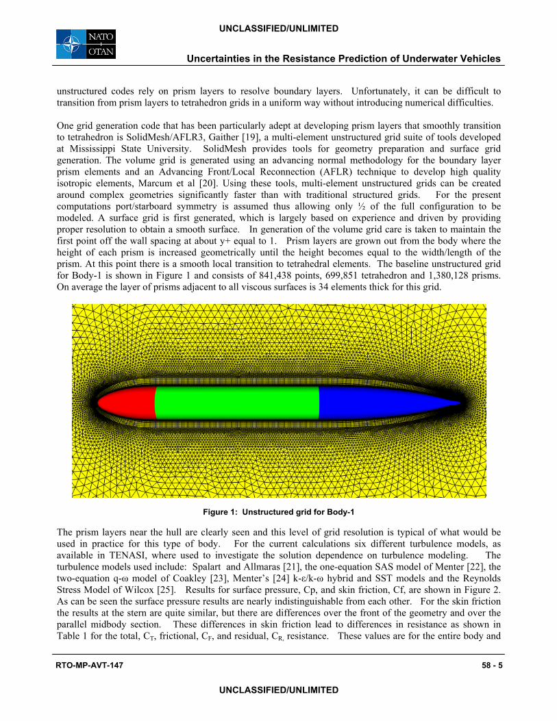
unstructured codes rely on prism layers to resolve boundary layers. Unfortunately, it can be difficult to transition from prism layers to tetrahedron grids in a uniform way without introducing numerical difficulties. One grid generation code that has been particularly adept at developing prism layers that smoothly transition to tetrahedron is SolidMesh/AFLR3, Gaither [19], a multi-element unstructured grid suite of tools developed at Mississippi State University. SolidMesh provides tools for geometry preparation and surface grid generation. The volume grid is generated using an advancing normal methodology for the boundary layer prism elements and an Advancing Front/Local Reconnection (AFLR) technique to develop high quality isotropic elements, Marcum et al [20]. Using these tools, multi-element unstructured grids can be created around complex geometries significantly faster than with traditional structured grids. For the present computations port/starboard symmetry is assumed thus allowing only ½ of the full configuration to be modeled. A surface grid is first generated, which is largely based on experience and driven by providing proper resolution to obtain a smooth surface. In generation of the volume grid care is taken to maintain the first point off the wall spacing at about y+ equal to 1. Prism layers are grown out from the body where the height of each prism is increased geometrically until the height becomes equal to the width/length of the prism. At this point there is a smooth local transition to tetrahedral elements. The baseline unstructured grid for Body-1 is shown in Figure 1 and consists of 841,438 points, 699,851 tetrahedron and 1,380,128 prisms. On average the layer of prisms adjacent to all viscous surfaces is 34 elements thick for this grid.

Figure 1: Unstructured grid for Body-1

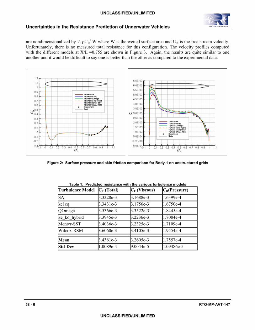
The prism layers near the hull are clearly seen and this level of grid resolution is typical of what would be used in practice for this type of body. For the current calculations six different turbulence models, as available in TENASI, where used to investigate the solution dependence on turbulence modeling. The turbulence models used include: Spalart and Allmaras [21], the one-equation SAS model of Menter [22], the two-equation q-ω model of Coakley [23], Menter’s [24] k-ε/k-ω hybrid and SST models and the Reynolds Stress Model of Wilcox [25]. Results for surface pressure, Cp, and skin friction, Cf, are shown in Figure 2. As can be seen the surface pressure results are nearly indistinguishable from each other. For the skin friction the results at the stern are quite similar, but there are differences over the front of the geometry and over the parallel midbody section. These differences in skin friction lead to differences in resistance as shown in Table 1 for the total, CT, frictional, CF, and residual, CR, resistance. These values are for the entire body and




58 - 6 RTO-MP-AVT-147

are nondimensionalized by ½ ρU∞2 W where W is the wetted surface area and U∞ is the free stream velocity.

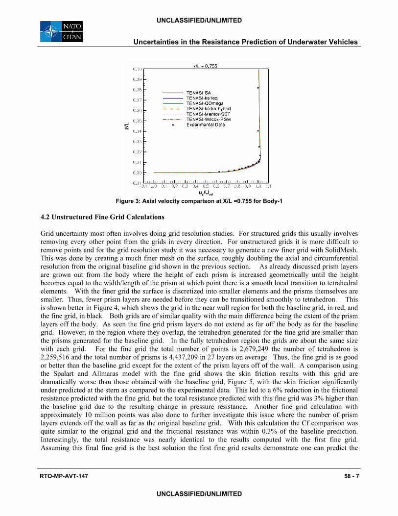
Unfortunately, there is no measured total resistance for this configuration. The velocity profiles computed with the different models at X/L =0.755 are shown in Figure 3. Again, the results are quite similar to one another and it would be difficult to say one is better than the other as compared to the experimental data.

Figure 2: Surface pressure and skin friction comparison for Body-1 on unstructured grids

Table 1: Predicted resistance with the various turbulence models

Turbulence Model CT (Total) CF (Viscous) CR(Pressure)

SA 3.3328e-3 3.1688e-3 1.6399e-4 ke1eq 3.3431e-3 3.1756e-3 1.6750e-4 QOmega 3.5366e-3 3.3522e-3 1.8445e-4 ke_ko_hybrid 3.3945e-3 3.2236e-3 1.7084e-4 Menter-SST 3.4036e-3 3.2325e-3 1.7109e-4 Wilcox-RSM 3.6060e-3 3.4105e-3 1.9554e-4

Mean 3.4361e-3 3.2605e-3 1.7557e-4 Std-Dev 1.0089e-4 9.0044e-5 1.09486e-5




RTO-MP-AVT-147 58 - 7

Figure 3: Axial velocity comparison at X/L =0.755 for Body-1

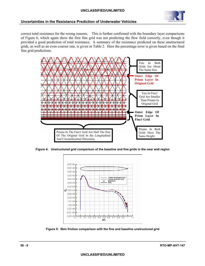
4.2 Unstructured Fine Grid Calculations Grid uncertainty most often involves doing grid resolution studies. For structured grids this usually involves removing every other point from the grids in every direction. For unstructured grids it is more difficult to remove points and for the grid resolution study it was necessary to generate a new finer grid with SolidMesh. This was done by creating a much finer mesh on the surface, roughly doubling the axial and circumferential resolution from the original baseline grid shown in the previous section. As already discussed prism layers are grown out from the body where the height of each prism is increased geometrically until the height becomes equal to the width/length of the prism at which point there is a smooth local transition to tetrahedral elements. With the finer grid the surface is discretized into smaller elements and the prisms themselves are smaller. Thus, fewer prism layers are needed before they can be transitioned smoothly to tetrahedron. This is shown better in Figure 4, which shows the grid in the near wall region for both the baseline grid, in red, and the fine grid, in black. Both grids are of similar quality with the main difference being the extent of the prism layers off the body. As seen the fine grid prism layers do not extend as far off the body as for the baseline grid. However, in the region where they overlap, the tetrahedron generated for the fine grid are smaller than the prisms generated for the baseline grid. In the fully tetrahedron region the grids are about the same size with each grid. For the fine grid the total number of points is 2,679,249 the number of tetrahedron is 2,259,516 and the total number of prisms is 4,437,209 in 27 layers on average. Thus, the fine grid is as good or better than the baseline grid except for the extent of the prism layers off of the wall. A comparison using the Spalart and Allmaras model with the fine grid shows the skin friction results with this grid are dramatically worse than those obtained with the baseline grid, Figure 5, with the skin friction significantly under predicted at the stern as compared to the experimental data. This led to a 6% reduction in the frictional resistance predicted with the fine grid, but the total resistance predicted with this fine grid was 3% higher than the baseline grid due to the resulting change in pressure resistance. Another fine grid calculation with approximately 10 million points was also done to further investigate this issue where the number of prism layers extends off the wall as far as the original baseline grid. With this calculation the Cf comparison was quite similar to the original grid and the frictional resistance was within 0.3% of the baseline prediction. Interestingly, the total resistance was nearly identical to the results computed with the first fine grid. Assuming this final fine grid is the best solution the first fine grid results demonstrate one can predict the




58 - 8 RTO-MP-AVT-147

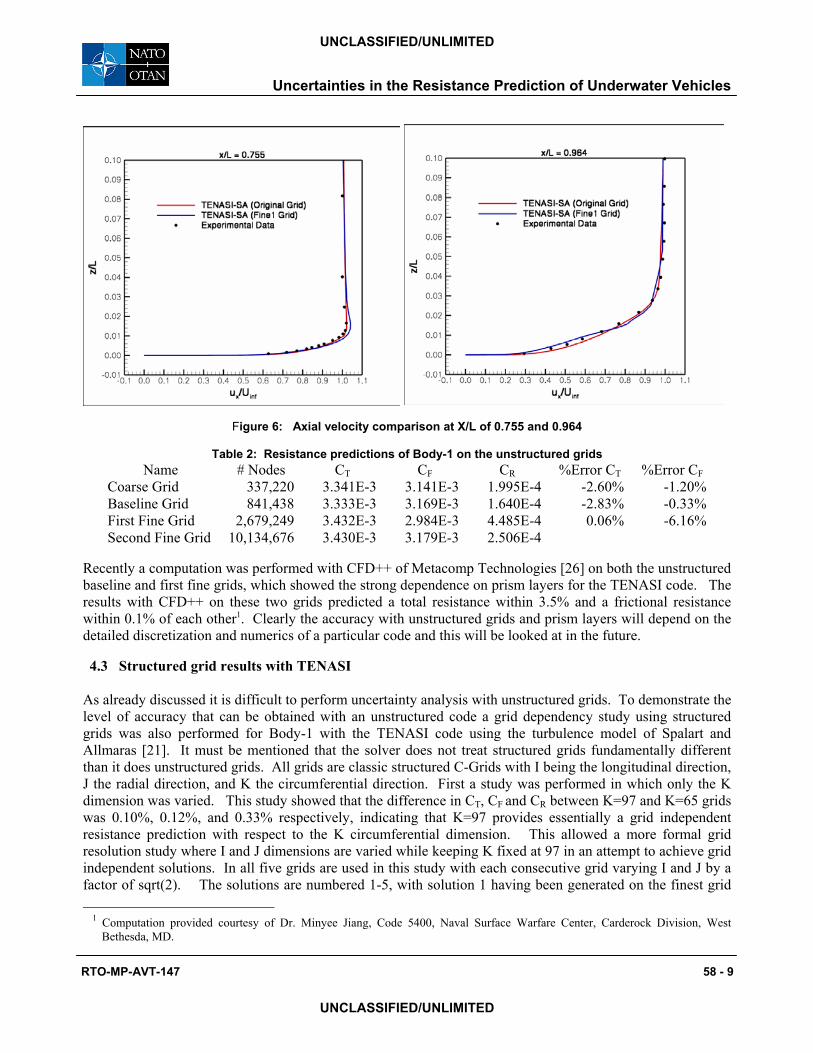
correct total resistance for the wrong reasons. This is further confirmed with the boundary layer comparisons of Figure 6, which again show the first fine grid was not predicting the flow field correctly, even though it provided a good prediction of total resistance. A summary of the resistance predicted on these unstructured grids, as well as an even coarser one, is given in Table 2. Here the percentage error is given based on the final fine grid predictions.

Figure 4: Unstructured grid comparison of the baseline and fine grids in the near wall region

Figure 5: Skin friction comparison with the fine and baseline unstructured grid

Outer Edge Of Prism Layer In Original Grid

Outer Edge Of Prism Layer In Fine1 Grid

Tets In Both Grids Are About The Same Size

Tets In Fine1 Grid Are Smaller Than Prisms In Original Grid

Prisms In Both Grids Have The Same Height

Prisms In The Fine1 Grid Are Half The Size Of The Original Grid In the Longitudinal And Circumferential Directions




RTO-MP-AVT-147 58 - 9

Figure 6: Axial velocity comparison at X/L of 0.755 and 0.964

Table 2: Resistance predictions of Body-1 on the unstructured grids Name # Nodes CT CF CR %Error CT %Error CF

Coarse Grid 337,220 3.341E-3 3.141E-3 1.995E-4 -2.60% -1.20%Baseline Grid 841,438 3.333E-3 3.169E-3 1.640E-4 -2.83% -0.33%First Fine Grid 2,679,249 3.432E-3 2.984E-3 4.485E-4 0.06% -6.16%Second Fine Grid 10,134,676 3.430E-3 3.179E-3 2.506E-4

Recently a computation was performed with CFD++ of Metacomp Technologies [26] on both the unstructured baseline and first fine grids, which showed the strong dependence on prism layers for the TENASI code. The results with CFD++ on these two grids predicted a total resistance within 3.5% and a frictional resistance within 0.1% of each other1. Clearly the accuracy with unstructured grids and prism layers will depend on the detailed discretization and numerics of a particular code and this will be looked at in the future. 4.3 Structured grid results with TENASI As already discussed it is difficult to perform uncertainty analysis with unstructured grids. To demonstrate the level of accuracy that can be obtained with an unstructured code a grid dependency study using structured grids was also performed for Body-1 with the TENASI code using the turbulence model of Spalart and Allmaras [21]. It must be mentioned that the solver does not treat structured grids fundamentally different than it does unstructured grids. All grids are classic structured C-Grids with I being the longitudinal direction, J the radial direction, and K the circumferential direction. First a study was performed in which only the K dimension was varied. This study showed that the difference in CT, CF and CR between K=97 and K=65 grids was 0.10%, 0.12%, and 0.33% respectively, indicating that K=97 provides essentially a grid independent resistance prediction with respect to the K circumferential dimension. This allowed a more formal grid resolution study where I and J dimensions are varied while keeping K fixed at 97 in an attempt to achieve grid independent solutions. In all five grids are used in this study with each consecutive grid varying I and J by a factor of sqrt(2). The solutions are numbered 1-5, with solution 1 having been generated on the finest grid

1 Computation provided courtesy of Dr. Minyee Jiang, Code 5400, Naval Surface Warfare Center, Carderock Division, West Bethesda, MD.




58 - 10 RTO-MP-AVT-147

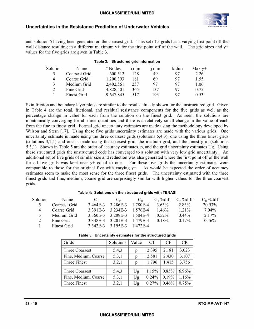
and solution 5 having been generated on the coarsest grid. This set of 5 grids has a varying first point off the wall distance resulting in a different maximum y+ for the first point off of the wall. The grid sizes and y+ values for the five grids are given in Table 3.

Table 3: Structured grid information

Skin friction and boundary layer plots are similar to the results already shown for the unstructured grid. Given in Table 4 are the total, frictional, and residual resistance components for the five grids as well as the percentage change in value for each from the solution on the finest grid. As seen, the solutions are montonically converging for all three quantities and there is a relatively small change in the value of each from the fine to finest grid. Formal grid uncertainty estimates are made using the methodology developed by Wilson and Stern [17]. Using these five grids uncertainty estimates are made with the various grids. One uncertainty estimate is made using the three coarsest grids (solutions 5,4,3), one using the three finest grids (solutions 3,2,1) and one is made using the coarsest grid, the medium grid, and the finest grid (solutions 5,3,1). Shown in Table 5 are the order of accuracy estimates, p, and the grid uncertainty estimates Ug. Using these structured grids the unstructured code has converged to a solution with very low grid uncertainty. An additional set of five grids of similar size and reduction was also generated where the first point off of the wall for all five grids was kept near y+ equal to one. For these five grids the uncertainty estimates were comparable to those for the original five with varying y+. As would be expected the order of accuracy estimates seem to make the most sense for the three finest grids. The uncertainty estimated with the three finest grids and fine, medium, coarse grid are surprisingly similar with higher values for the three coarsest grids.

Table 4: Solutions on the structured grids with TENASI

Solution Name CT CF CR CT %diff CF %diff CR %diff 5 Coarsest Grid 3.464E-3 3.286E-3 1.780E-4 3.63% 2.83% 20.93% 4 Coarse Grid 3.391E-3 3.234E-3 1.576E-4 1.46% 1.21% 7.04% 3 Medium Grid 3.360E-3 3.209E-3 1.504E-4 0.52% 0.44% 2.17% 2 Fine Grid 3.348E-3 3.201E-3 1.479E-4 0.18% 0.17% 0.46% 1 Finest Grid 3.342E-3 3.195E-3 1.472E-4

Table 5: Uncertainty estimates for the structured grids

Grids Solutions Value CT CF CR

Three Coarsest 5,4,3 p 2.395 2.181 3.023 Fine, Medium, Coarse 5,3,1 p 2.581 2.430 3.107 Three Finest 3,2,1 p 1.796 1.415 3.756

Three Coarsest 5,4,3 Ug 1.15% 0.85% 6.96% Fine, Medium, Coarse 5,3,1 Ug 0.24% 0.19% 1.16% Three Finest 3,2,1 Ug 0.27% 0.46% 0.75%

Solution Name # Nodes i dim j dim k dim Max y+ 5 Coarsest Grid 600,512 128 49 97 2.26 4 Coarse Grid 1,200,393 181 69 97 1.55 3 Medium Grid 2,402,561 257 97 97 1.06 2 Fine Grid 4,828,501 365 137 97 0.75 1 Finest Grid 9,647,845 517 193 97 0.53




RTO-MP-AVT-147 58 - 11

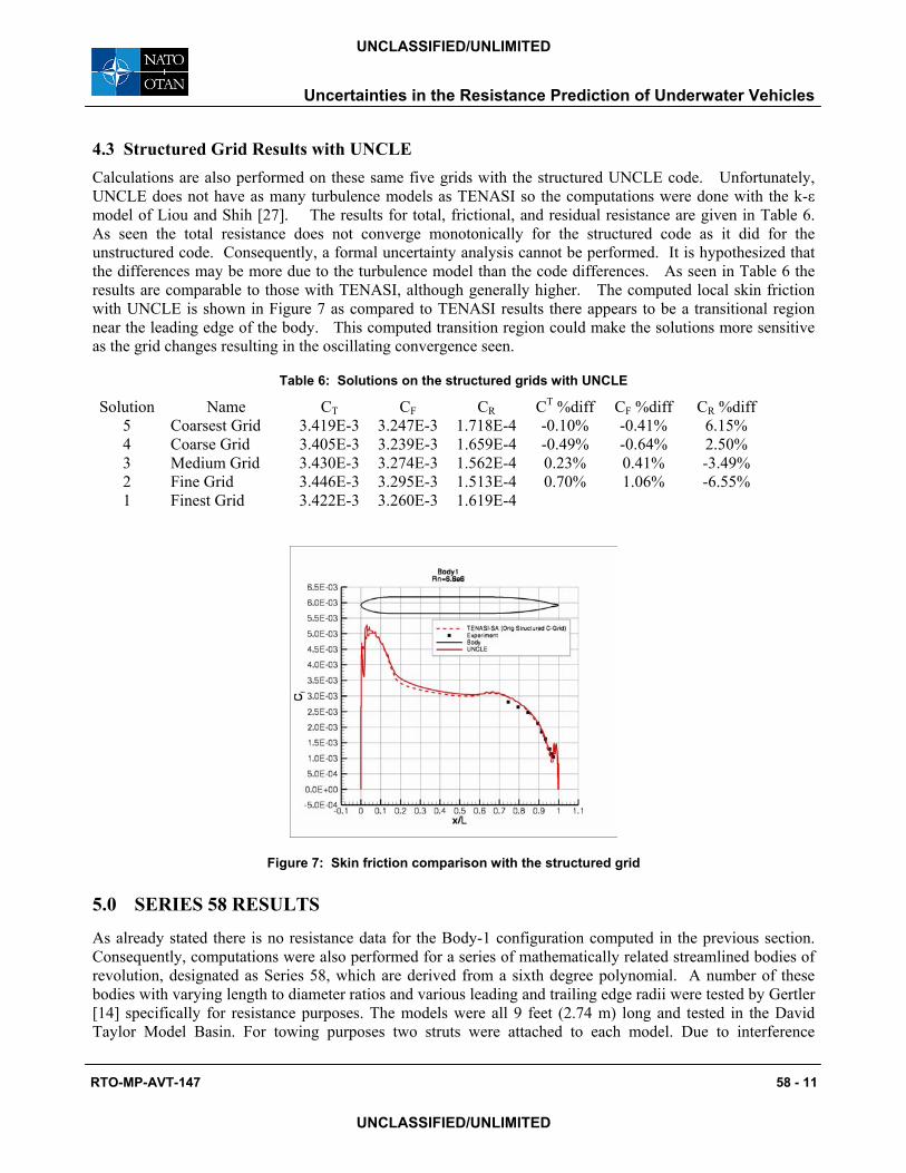
4.3 Structured Grid Results with UNCLE Calculations are also performed on these same five grids with the structured UNCLE code. Unfortunately, UNCLE does not have as many turbulence models as TENASI so the computations were done with the k-ε model of Liou and Shih [27]. The results for total, frictional, and residual resistance are given in Table 6. As seen the total resistance does not converge monotonically for the structured code as it did for the unstructured code. Consequently, a formal uncertainty analysis cannot be performed. It is hypothesized that the differences may be more due to the turbulence model than the code differences. As seen in Table 6 the results are comparable to those with TENASI, although generally higher. The computed local skin friction with UNCLE is shown in Figure 7 as compared to TENASI results there appears to be a transitional region near the leading edge of the body. This computed transition region could make the solutions more sensitive as the grid changes resulting in the oscillating convergence seen.

Table 6: Solutions on the structured grids with UNCLE

Solution Name CT CF CR CT %diff CF %diff CR %diff 5 Coarsest Grid 3.419E-3 3.247E-3 1.718E-4 -0.10% -0.41% 6.15% 4 Coarse Grid 3.405E-3 3.239E-3 1.659E-4 -0.49% -0.64% 2.50% 3 Medium Grid 3.430E-3 3.274E-3 1.562E-4 0.23% 0.41% -3.49% 2 Fine Grid 3.446E-3 3.295E-3 1.513E-4 0.70% 1.06% -6.55% 1 Finest Grid 3.422E-3 3.260E-3 1.619E-4

Figure 7: Skin friction comparison with the structured grid

5.0 SERIES 58 RESULTS

As already stated there is no resistance data for the Body-1 configuration computed in the previous section. Consequently, computations were also performed for a series of mathematically related streamlined bodies of revolution, designated as Series 58, which are derived from a sixth degree polynomial. A number of these bodies with varying length to diameter ratios and various leading and trailing edge radii were tested by Gertler [14] specifically for resistance purposes. The models were all 9 feet (2.74 m) long and tested in the David Taylor Model Basin. For towing purposes two struts were attached to each model. Due to interference




58 - 12 RTO-MP-AVT-147

between the models and the towing struts the measured resistance is higher than on the bare bodies themselves. Consequently, a pair of dummy struts, similar to the towing struts, were also constructed and mounted at ninety degrees to the original struts. Tests were conducted with and without the dummy struts with the difference giving an estimate of strut-interference effects. This strut-interference value can then be subtracted from the resistance obtained for the body of revolution with towing struts to obtain an estimate of the resistance of the body of revolution alone. Different values of strut interference coefficient are obtained for the different models, but it is assumed the value for each individual model is independent of Reynolds number. The experimental data as presented here has the strut-interference coefficient removed for comparison with the bare body calculations. The experimental measurements were conducted both with smooth models and with a 1/2 inch (1.27 cm) sand strip placed at X/L = 0.05 to better stimulate transition to turbulence. The models were towed at a depth of 9 feet (2.74m), which was thought to minimize free surface effects. Calculations are presented for a range of Reynolds numbers ranging from 2.0x106 to 25.0x106, based on body length, which covers the range over which the experiments were performed. No attempt is made to model transition in the calculations. The models computed are 4159, 4158, and 4155 corresponding to length to diameter ratios of 10, 8, and 5, respectively. 5.1 Unstructured grid results with TENASI The unstructured grids for these geometries are topologically similar to that of Body-1, shown in Figure 1, and the number of grid points for each are given in Table 7. Although Model 4155 has the largest wetted surface area, because the L/D ratio is the smallest it requires the fewest number of grid cells on the surface to properly define the surface with well behaved near equal sided cells. The larger L/D geometries need more cells on the surface, in order to avoid large aspect ratio cells, which in turn lead to more cells in general in the flow volume. Basically, the grids are generated using 41 nodes circumferentially for the half body with adjustments at the ends to adequately resolve the leading and trailing edge radii. For each Model the grid was generated so that at the highest Reynolds number the first point off of the wall would be at a maximum y+ value of approximately 1. This grid was then used for all of the lower Reynolds number calculations as well. Computations are performed with TENASI using three turbulence models: Spalart and Allmaras [21], the one-equation SAS model of Menter [22] and the two-equation q-ω model of Coakley [23].

Table 7: Unstructured grids used for Series 58 calculations

Model L/D # Points # Tetrahedron # Prisms

4159 10 944,109 796,235 1,548,1204158 8 851,196 662,424 1,415,3984155 5 522,969 434,004 858,326

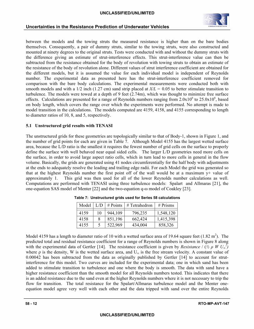
Model 4159 has a length to diameter ratio of 10 with a wetted surface area of 19.64 square feet (1.82 m2). The predicted total and residual resistance coefficient for a range of Reynolds numbers is shown in Figure 8 along with the experimental data of Gertler [14]. The resistance coefficient is given by Resistance / (½ ρ W U∞

2) where ρ is the density, W is the wetted surface area, and U∞ is the free stream velocity. A constant value of 0.00042 has been subtracted from the data as originally published by Gertler [14] to account for strut-interference for this model. Two curves are included for the experimental data; one in which sand has been added to stimulate transition to turbulence and one where the body is smooth. The data with sand have a higher resistance coefficient than the smooth model for all Reynolds numbers tested. This indicates that there is an added resistance due to the sand even at the higher Reynolds numbers where it is not necessary to trip the flow for transition. The total resistance for the Spalart/Allmaras turbulence model and the Menter one-equation model agree very well with each other and the data tripped with sand over the entire Reynolds




RTO-MP-AVT-147 58 - 13

number regime. The q-ω results tend to be high. The computed residual resistance largely lies between the experimental results with and without sand. In the experiment the residual resistance has been obtained by subtracting the frictional resistance, estimated with the Schoenherr formula, from the measured total resistance. Clearly the residual resistance is Reynolds number dependent at the lower Reynolds numbers and even at the highest Reynolds numbers the residual resistance is still varying.

Figure 8: Total and residual resistance for Model 4159

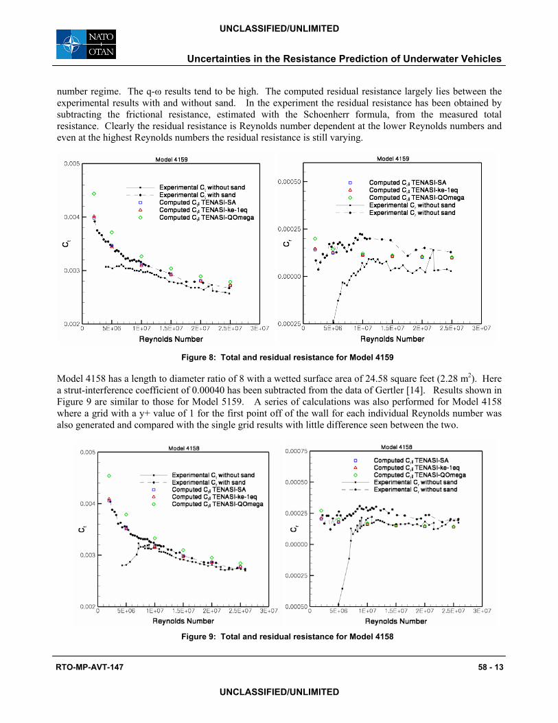
Model 4158 has a length to diameter ratio of 8 with a wetted surface area of 24.58 square feet (2.28 m2). Here a strut-interference coefficient of 0.00040 has been subtracted from the data of Gertler [14]. Results shown in Figure 9 are similar to those for Model 5159. A series of calculations was also performed for Model 4158 where a grid with a y+ value of 1 for the first point off of the wall for each individual Reynolds number was also generated and compared with the single grid results with little difference seen between the two.





58 - 14 RTO-MP-AVT-147

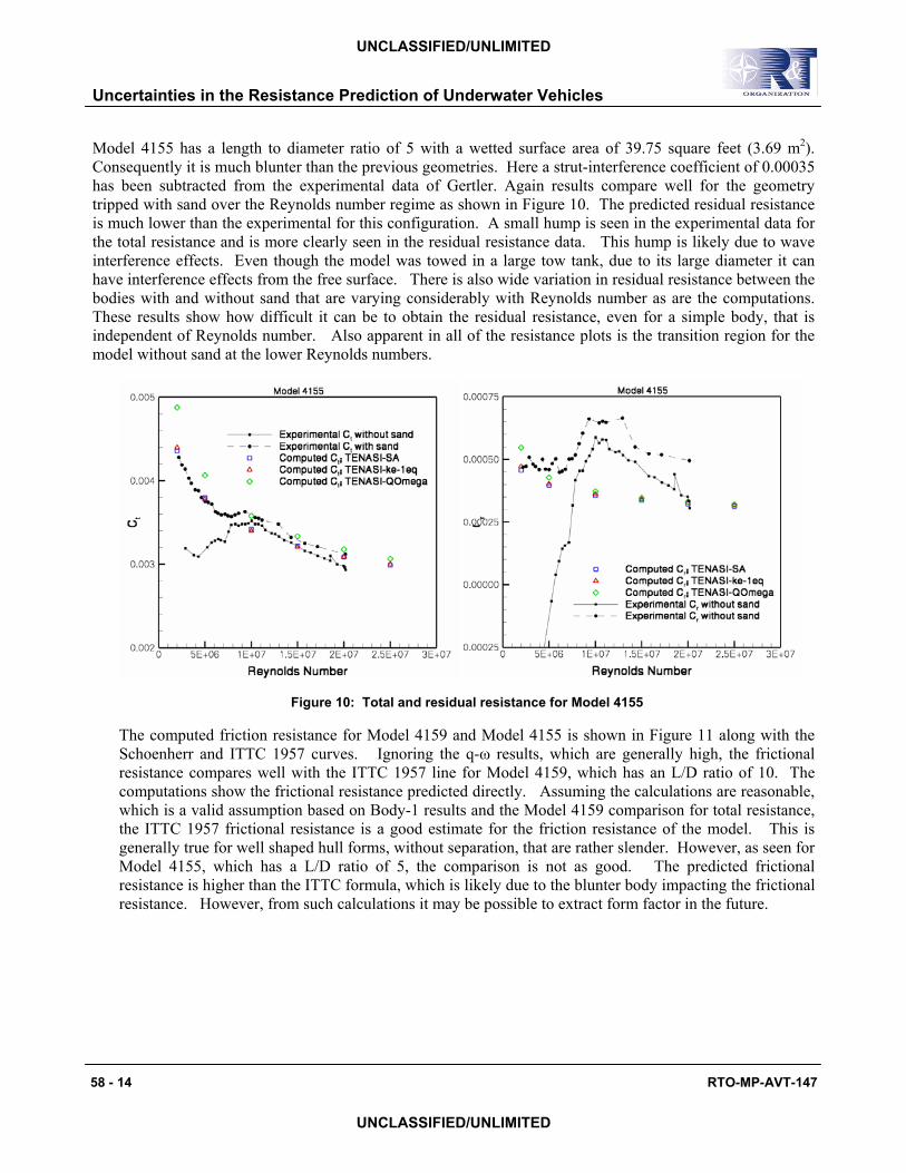
Model 4155 has a length to diameter ratio of 5 with a wetted surface area of 39.75 square feet (3.69 m2). Consequently it is much blunter than the previous geometries. Here a strut-interference coefficient of 0.00035 has been subtracted from the experimental data of Gertler. Again results compare well for the geometry tripped with sand over the Reynolds number regime as shown in Figure 10. The predicted residual resistance is much lower than the experimental for this configuration. A small hump is seen in the experimental data for the total resistance and is more clearly seen in the residual resistance data. This hump is likely due to wave interference effects. Even though the model was towed in a large tow tank, due to its large diameter it can have interference effects from the free surface. There is also wide variation in residual resistance between the bodies with and without sand that are varying considerably with Reynolds number as are the computations. These results show how difficult it can be to obtain the residual resistance, even for a simple body, that is independent of Reynolds number. Also apparent in all of the resistance plots is the transition region for the model without sand at the lower Reynolds numbers.


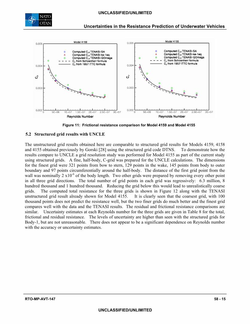
The computed friction resistance for Model 4159 and Model 4155 is shown in Figure 11 along with the Schoenherr and ITTC 1957 curves. Ignoring the q-ω results, which are generally high, the frictional resistance compares well with the ITTC 1957 line for Model 4159, which has an L/D ratio of 10. The computations show the frictional resistance predicted directly. Assuming the calculations are reasonable, which is a valid assumption based on Body-1 results and the Model 4159 comparison for total resistance, the ITTC 1957 frictional resistance is a good estimate for the friction resistance of the model. This is generally true for well shaped hull forms, without separation, that are rather slender. However, as seen for Model 4155, which has a L/D ratio of 5, the comparison is not as good. The predicted frictional resistance is higher than the ITTC formula, which is likely due to the blunter body impacting the frictional resistance. However, from such calculations it may be possible to extract form factor in the future.




RTO-MP-AVT-147 58 - 15

Figure 11: Frictional resistance comparison for Model 4159 and Model 4155

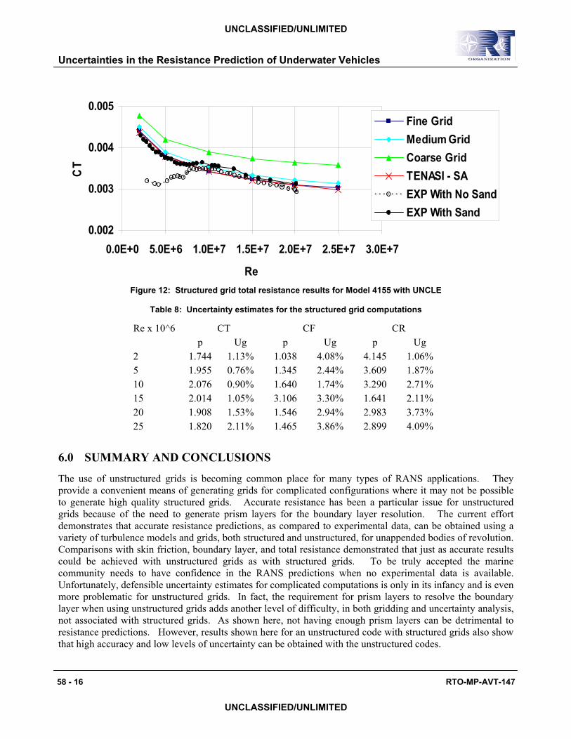
5.2 Structured grid results with UNCLE The unstructured grid results obtained here are comparable to structured grid results for Models 4159, 4158 and 4155 obtained previously by Gorski [28] using the structured grid code DTNS. To demonstrate how the results compare to UNCLE a grid resolution study was performed for Model 4155 as part of the current study using structured grids. A fine, half-body, C-grid was prepared for the UNCLE calculations. The dimensions for the finest grid were 321 points from bow to stern, 129 points in the wake, 145 points from body to outer boundary and 97 points circumferentially around the half-body. The distance of the first grid point from the wall was nominally 2 x10-6 of the body length. Two other grids were prepared by removing every other point in all three grid directions. The total number of grid points in each grid was regressively: 6.3 million, 8 hundred thousand and 1 hundred thousand. Reducing the grid below this would lead to unrealistically coarse grids. The computed total resistance for the three grids is shown in Figure 12 along with the TENASI unstructured grid result already shown for Model 4155. It is clearly seen that the coarsest grid, with 100 thousand points does not predict the resistance well, but the two finer grids do much better and the finest grid compares well with the data and the TENASI results. The residual and frictional resistance comparisons are similar. Uncertainty estimates at each Reynolds number for the three grids are given in Table 8 for the total, frictional and residual resistance. The levels of uncertainty are higher than seen with the structured grids for Body-1, but are not unreasonable. There does not appear to be a significant dependence on Reynolds number with the accuracy or uncertainty estimates.




58 - 16 RTO-MP-AVT-147

0.002

0.003

0.004

0.005

0.0E+0 5.0E+6 1.0E+7 1.5E+7 2.0E+7 2.5E+7 3.0E+7

Re

CT

Fine GridMedium GridCoarse GridTENASI - SAEXP With No SandEXP With Sand

Figure 12: Structured grid total resistance results for Model 4155 with UNCLE

Table 8: Uncertainty estimates for the structured grid computations

Re x 10^6 CT CF CR p Ug p Ug p Ug 2 1.744 1.13% 1.038 4.08% 4.145 1.06% 5 1.955 0.76% 1.345 2.44% 3.609 1.87% 10 2.076 0.90% 1.640 1.74% 3.290 2.71% 15 2.014 1.05% 3.106 3.30% 1.641 2.11% 20 1.908 1.53% 1.546 2.94% 2.983 3.73% 25 1.820 2.11% 1.465 3.86% 2.899 4.09%

6.0 SUMMARY AND CONCLUSIONS

The use of unstructured grids is becoming common place for many types of RANS applications. They provide a convenient means of generating grids for complicated configurations where it may not be possible to generate high quality structured grids. Accurate resistance has been a particular issue for unstructured grids because of the need to generate prism layers for the boundary layer resolution. The current effort demonstrates that accurate resistance predictions, as compared to experimental data, can be obtained using a variety of turbulence models and grids, both structured and unstructured, for unappended bodies of revolution. Comparisons with skin friction, boundary layer, and total resistance demonstrated that just as accurate results could be achieved with unstructured grids as with structured grids. To be truly accepted the marine community needs to have confidence in the RANS predictions when no experimental data is available. Unfortunately, defensible uncertainty estimates for complicated computations is only in its infancy and is even more problematic for unstructured grids. In fact, the requirement for prism layers to resolve the boundary layer when using unstructured grids adds another level of difficulty, in both gridding and uncertainty analysis, not associated with structured grids. As shown here, not having enough prism layers can be detrimental to resistance predictions. However, results shown here for an unstructured code with structured grids also show that high accuracy and low levels of uncertainty can be obtained with the unstructured codes.




RTO-MP-AVT-147 58 - 17

One great expectation for RANS codes is to compute the full scale performance of ships. Of course, before we can have confidence in full scale predictions we need to validate our prediction capability with model scale experiments. A significant experimental effort may be required to provide the necessary data, both of local and global quantities, for code and process validation. Many historic data sets are not reliable for CFD validation because of the poor data quality or insufficient documentation of the actual experimental conditions. Efforts in recent years have often attempted to acquire higher quality data specifically for CFD validation. However, skin friction data, which is very relevant to resistance, is particularly lacking. Additionally, the level of CFD validation today often encompasses only a few single point calculations rather than systematic evaluation of the ability to predict the measured flow physics over a range of conditions or increasingly complicated geometry variants. RANS is here to stay and will be used to address all types of problems on all types of grids in the future. The community needs to develop ways to both demonstrate the accuracy of the codes as well as to have confidence in the codes when no data exists. Developing methods for uncertainty analysis is a first step to developing this confidence, but the community has a long way to go before computations are as accepted as experiments.

7.0 REFERENCES

[1] Froude, W. M., “On Experiments with H.M.S. Greyhound,” Trans. INA, Vol. 15, pp. 36 – 73, 1874.

[2] Schoenherr, K.E., “Resistance of Flat Surfaces Moving Through a Fluid,” Transactions of the Society of Naval Architects, Vol. 40, 1932.

[3] Hadler, J. B., “Coefficients for International Towing Tank Conference 1957 Model-Ship Correlation Line,” The David Taylor Model Basin, Report 1185, April 1958.

[4] ITTC, “Report of the Resistance and Flow Committee,” Proc. 21st ITTC, Trondheim, Norway, 1996.

[5] Gorski, J. J. and Coleman, R. M., “Use of RANS Calculations in the Design of a Submarine Sail,” Proc. NATO RTO Applied Vehicle Technology Panel Spring 2002 Meeting, Paris, France, April 2002.

[6] Gorski, J. J., Haussling, H. J., Percival, A. S., Shaughnessy, J. J. and Buley, G. M., “The Use of a RANS Code in the Design and Analysis of a Naval Combatant,” Proc. 24th Symposium on Naval Hydrodynamics, Fukuoka, Japan, July 2002b.

[7] Eça, L. and Hoekstra, M., (editors), 2nd Workshop on CFD Uncertainty Analysis, Lisbon, October, 2006.

[8] Roache, P., Verification and Validation in Computational Science and Engineering, Hermosa Publishers, Albuquerque, NM, 1998.

[9] Gorski, J. J., Miller, R. W., and Coleman, R. M., “An Investigation of Propeller Inflow for Naval Surface Combatants,” Proc. 25th Symposium on Naval Hydrodynamics, St. John’s, Newfoundland, Canada, Aug. 2004.

[10] Ebert, M. P., Gorski, J. J., and Coleman, R. M., “Viscous Flow Calculations of Waterjet Propelled Ships,” Proc. 8th Int. Conf. on Numerical Ship Hydrodynamics, Busan, Korea, Sept., 2003.

[11] Sreenivas, K., Taylor, L.K., and Briley, W.R., “A Global Preconditioner for Viscous Flow Simulations at All Mach Numbers,” AIAA Paper 2006-3852, June 2006.




58 - 18 RTO-MP-AVT-147

[12] Taylor, L. K. and D. L. Whitfield, “Unsteady Three-Dimensional Incompressible Euler and Navier-Stokes Solver for Stationary and Dynamic Grids,” AIAA Paper No. 91-1650, June, 1991.

[13] Huang, T. T., N. Santelli, and G. Belt, “Stern Boundary-Layer Flow on Axisymmetric Bodies,” Proceedings of the 12th Symposium on Naval Hydrodynamics, Washington, D.C., June 1978.

[14] Gertler, M., “Resistance Experiments on a Systematic Series of Streamlined Bodies of Revolution - For Application to the Design of High-Speed Submarines,” The David Taylor Model Basin, Report C-297, April 1950.

[15] Hyams, D.G., “An Investigation of Parallel Implicit Solution Algorithms for Incompressible Flows on Unstructured Topologies,” Ph. D. Dissertation, Department of Mechanical Engineering, Mississippi State University, Mississippi State, MS, May 2000.

[16] Taylor, L. K., A. Arabshahi, and D. L. Whitfield, “Unsteady Three-Dimensional Incompressible Navier-Stokes Computations for a Prolate Spheroid Undergoing Time-Dependent Maneuvers,” AIAA Paper No. 95-0313, Jan. 1995.

[17] Wilson, R. and Stern, F., “Verification and Validation for RANS Simulation of a Naval Surface Combatant,” AIAA Paper 2002-0904, 2002.

[18] Ebert, M. P. and Gorski, J. J., “A Verification and Validation Procedure for Computational Fluid Dynamics Solutions,” NSWCCD – 50 – TR – 2001/0006, Feb., 2001.

[19] Gaither, A. J., “A Solid Modeling Topology Data Structure for General Grid Generation,” Master’s thesis, Mississippi State University, 1997.

[20] Marcum, D. L., and A. J. Gaither, “Mixed Element Type Unstructured Grid Generation for Viscous Flow Applications,” AIAA Paper No. 99-3252, June 1999.

[21] Spalart, P.R., and Allmaras, S.R., “A One-Equation Turbulence Model for Aerodynamic Flows,” AIAA Paper 1992-0439, January 1992.

[22] Menter, F.R., Kuntz, M., and Bender, R., “A Scale-Adaptive Simulation Model for Turbulent Flow Predictions,” AIAA Paper 2003-0767, January 2003.

[23] Coakley, T. J., “Turbulence Methods for the Compressible Navier-Stokes Equations,” AIAA Paper No. 83-1693, 1983.

[24] Menter, F.R., “Two-Equation Eddy Viscosity Turbulence Models for Engineering Applications,” AIAA Journal, Vol. 32, 1994, pp. 1598-1605.

[25] Wilcox, D.C., Turbulence Modeling for CFD, 2nd ed., KNI, Inc., Anaheim, California, 2000.

[26] Metacomp Technologies, http://www.metacomptech.com

[27] Liou, W., and Shih, T-H., “Transonic Turbulent Flow Predictions with New Two-Equation Turbulence Models,” NASA Contractor Report 198444, Jan. 1996.

[28] Gorski, J. J., “Drag Calculations of Unappended Bodies of Revolution,” CRDKNSWC/HD-1362-07, Naval Surface Warfare Center, Carderock Division, West Bethesda, MD, May 1988.



Documents

Uncertainties in the Resistance Prediction of Underwater ... Meeting Proceedings/RTO... · Uncertainties in the Resistance Prediction of Underwater Vehicles ... Uncertainties in the