INFORMATION BULLETIN

UNDERSTANDING DETECTION CAPABILITY: LoB, LoD AND LoQ IN THE CLINICAL LABORATORY.

OVERVIEW

HISTORY

Detection capability is a broad term that relates to measurement accuracy. It has not always been necessary to

assess the accuracy and precision in measuring clinical analytes. Historically, the clinical decision points for most

analytes have been at concentrations much higher than the analytical limitations of the methods. For example,

the lower performance limits of methods for sodium and glucose have always been far below concentrations

where clinical decisions are made. Detection capability becomes exceedingly important for analytes such as

troponin, PSA and hCG, where most individuals have very low concentrations and the detection limits of the

methods are near the clinical decision limits. It is important to characterize low-end method performance for

analytes such as these in order for manufacturers to be assured that quality test methods have been developed

and for laboratories to trust that accurate patient results will be reported. This bulletin provides an overview of

detection capability with specific examples of statistical methods to assess accuracy and precision. The statistics

described are meant to be established by the manufacturer during development of the assay, however, laboratories

may wish to verify these in their institution as they prepare to implement a new test method. Additionally, these

statistics have application in the verification of analytical measuring range for immunoassays.

Analytical sensitivity was used to describe the upper limit of test results expected when testing a sample

containing no analyte. This statistic has no practical application alone, since there is no analyte in the sample.

It is difficult to apply this statistic to anything other than the measuring system. Analytical sensitivity is described

as a concentration limit, above which the user expects the observed signal to be the result of analyte presence,

in other words, the level at which the measured value is reflective of true analyte and not simply noise in the

system. Analytical sensitivity is typically calculated by repeatedly testing a blank (sample containing no analyte)

and determining a limit either 2 or 3 standard deviations (SD) above the observed mean. The number of replicates,

whether 2 or 3 SD is appropriate, and other details have not been established by consensus.

Functional sensitivity is a term that refers to measurement accuracy with a stated imprecision. The concept was

first applied to thyroid-stimulating hormone (TSH) assay, where “generations” of TSH assays were defined by the

concentration of TSH that could be measured at ≤20% coefficient of variance (CV). A CV of ≤10% is considered the

desired level of imprecision for other analytes, such as troponin. While functional sensitivity is related in a more

practical sense to clinical sample testing, there is no consensus protocol for establishing this statistic.

LAB FORWARD

DEFINITIONS

The preferred terms used to describe the detection capability of a measurement system are Limit of Blank (LoB), Limit of Detection (LoD) and Limit of

Quantitation (LoQ).

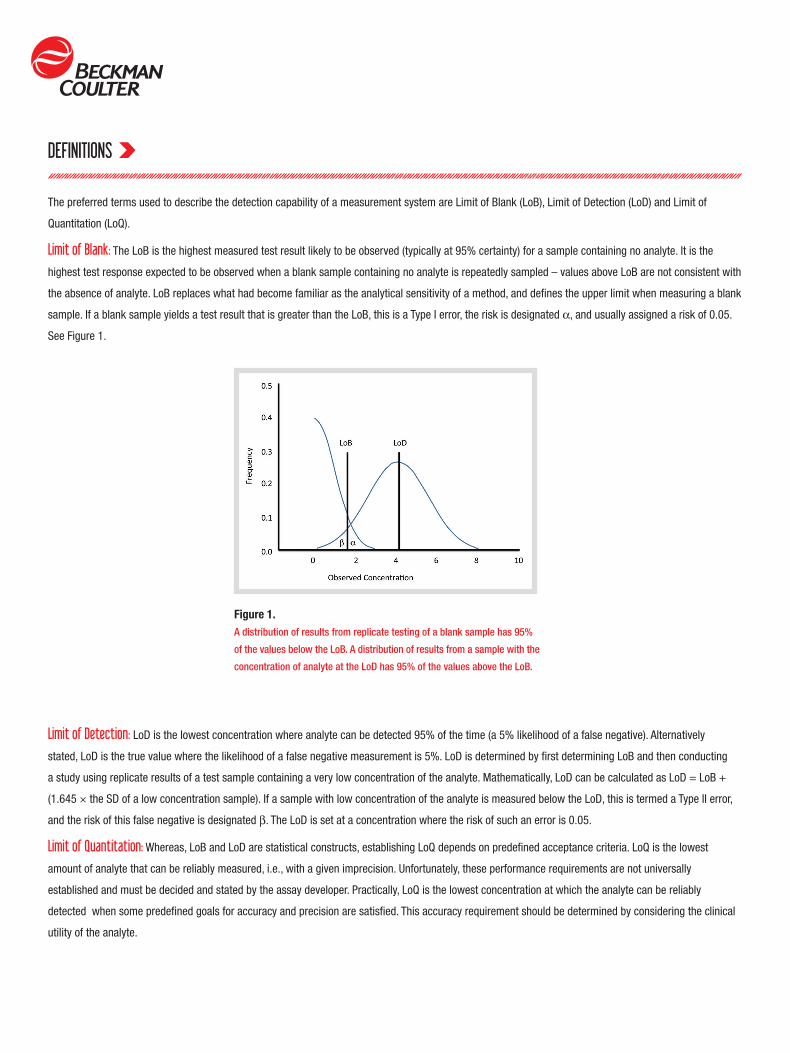
Limit of Blank: The LoB is the highest measured test result likely to be observed (typically at 95% certainty) for a sample containing no analyte. It is the

highest test response expected to be observed when a blank sample containing no analyte is repeatedly sampled – values above LoB are not consistent with

the absence of analyte. LoB replaces what had become familiar as the analytical sensitivity of a method, and defines the upper limit when measuring a blank

sample. If a blank sample yields a test result that is greater than the LoB, this is a Type I error, the risk is designated α, and usually assigned a risk of 0.05.

See Figure 1.

Limit of Detection: LoD is the lowest concentration where analyte can be detected 95% of the time (a 5% likelihood of a false negative). Alternatively

stated, LoD is the true value where the likelihood of a false negative measurement is 5%. LoD is determined by first determining LoB and then conducting

a study using replicate results of a test sample containing a very low concentration of the analyte. Mathematically, LoD can be calculated as LoD = LoB +

(1.645 × the SD of a low concentration sample). If a sample with low concentration of the analyte is measured below the LoD, this is termed a Type II error,

and the risk of this false negative is designated β. The LoD is set at a concentration where the risk of such an error is 0.05.

Limit of Quantitation: Whereas, LoB and LoD are statistical constructs, establishing LoQ depends on predefined acceptance criteria. LoQ is the lowest

amount of analyte that can be reliably measured, i.e., with a given imprecision. Unfortunately, these performance requirements are not universally

established and must be decided and stated by the assay developer. Practically, LoQ is the lowest concentration at which the analyte can be reliably

detected when some predefined goals for accuracy and precision are satisfied. This accuracy requirement should be determined by considering the clinical

utility of the analyte.

Figure 1.A distribution of results from replicate testing of a blank sample has 95%

of the values below the LoB. A distribution of results from a sample with the

concentration of analyte at the LoD has 95% of the values above the LoB.

SAMPLES TO CALCULATE LoB, LoD AND LoQ

PROTOCOLS TO CALCULATE LoB AND LoD

Blank Samples: Blank samples (containing no analyte) are used to establish the LoB. Ideally, the blank samples used should be natural, e.g., native serum,

and not an artificial matrix such as buffer. For therapeutic drugs, serum from an individual not medicated with the drug can be used. For endogenous

analytes, samples can be stripped, enzyme-treated, adsorbed with charcoal, antibody-precipitated, etc., to produce zero-analyte samples. The exact

minimum number of required blank replicate test results can be determined statistically, although four to five samples with 60 total replicates is usually

considered adequate.

Low-level Samples: Low-level samples are used to establish the LoD. The samples should be natural (e.g., native serum) as artificial or spiked samples may

behave differently in the measurement system. The number of samples and the concentrations depend on the protocol used (see below). Developers usually

have an initial estimate of the LoD. Sample concentrations should bracket this value.

Classical: The traditional approach for establishing LoB and LoD is based on the CLSI document EP17-A2. LoB is determined by repeatedly measuring the

blank sample using multiple reagent lots over multiple days. More rigorous testing could use multiple analyzers, with multiple calibrations, etc. The developer

must decide between parametric and nonparametric techniques, depending on the distribution of test results. If the test results have a normal distribution,

the mean and SD are determined and LoB can be calculated as:

LoB = Meanblank + cpSDblank

Because the SDblank is a biased estimate and not the true population SD, a correcting multiplier (cp) is used.

where cp is a multiplier to correct the SD estimate, B is the number of blank test results, and K is the number of blank samples. If the data is not normally

distributed, a nonparametric method should be used. A simple rank ordering method can be used to sort the data, then the ranked position of the 95th

percentile can be calculated:

Rank position = 0.5 + B(0.95)

For example, with 80 test results, the calculation is:

Rank position = 0.5 + 80(0.95) = 76.5

Because the resulting rank is not a whole integer, the results corresponding to the 76th and 77th ranked numbers are averaged to derive the LoD.

This protocol assumes the variability of the test method is nearly constant at concentrations near the LoD. At least four low level samples are needed for LoD

determination. These samples should be near the estimated LoD, typically one to five times the estimated LoB. The exact concentrations of the samples are

not important, because it is the SD that is used to calculate the LoD. LoD is derived from the calculated LoB and an expression of the determined SD of the

low level sample results.

LoD = LoB + cpSDlow level

where cp is the correcting multiplier, L is the total number of low level sample results, and J is the number of low level samples used.

PROTOCOLS TO CALCULATE LoB AND LoD

PROTOCOLS TO CALCULATE LoQ

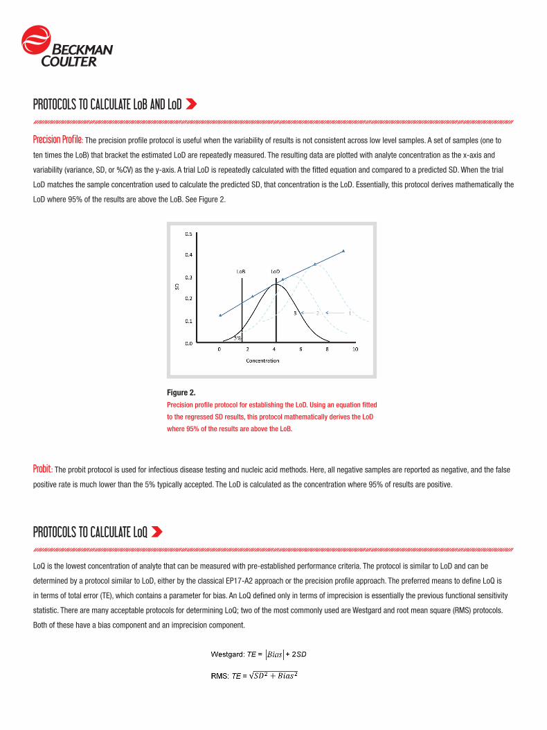
Precision Profile: The precision profile protocol is useful when the variability of results is not consistent across low level samples. A set of samples (one to

ten times the LoB) that bracket the estimated LoD are repeatedly measured. The resulting data are plotted with analyte concentration as the x-axis and

variability (variance, SD, or %CV) as the y-axis. A trial LoD is repeatedly calculated with the fitted equation and compared to a predicted SD. When the trial

LoD matches the sample concentration used to calculate the predicted SD, that concentration is the LoD. Essentially, this protocol derives mathematically the

LoD where 95% of the results are above the LoB. See Figure 2.

LoQ is the lowest concentration of analyte that can be measured with pre-established performance criteria. The protocol is similar to LoD and can be

determined by a protocol similar to LoD, either by the classical EP17-A2 approach or the precision profile approach. The preferred means to define LoQ is

in terms of total error (TE), which contains a parameter for bias. An LoQ defined only in terms of imprecision is essentially the previous functional sensitivity

statistic. There are many acceptable protocols for determining LoQ; two of the most commonly used are Westgard and root mean square (RMS) protocols.

Both of these have a bias component and an imprecision component.

Probit: The probit protocol is used for infectious disease testing and nucleic acid methods. Here, all negative samples are reported as negative, and the false

positive rate is much lower than the 5% typically accepted. The LoD is calculated as the concentration where 95% of results are positive.

Figure 2.Precision profile protocol for establishing the LoD. Using an equation fitted

to the regressed SD results, this protocol mathematically derives the LoD

where 95% of the results are above the LoB.

PROTOCOLS TO CALCULATE LoQ

There are several acceptable ways to estimate bias. Assigned standards are rarely available at the concentration of LoQ. Diluted or spiked samples are

acceptable, as long as the samples are commutable to actual patient samples. The design of the protocol can vary widely, but typically has replicates

sampled over multiple days using more than one analyzer, and more than one reagent lot. Multiple calibrations, etc., can be added to increase variability for

a more robust study design.

Similar to the LoD determination, a precision profile approach is typically used for LoQ. The main difference is the selection of low level samples, which must

have known concentrations. After all data has been collected, the LoQ is determined by the following steps.

1. Calculate the mean (x) and SD for each sample for all replicates within each reagent lot.

2. Caluclate the bias: Bias = x - R

where R is the known (assigned) value for the sample.

3. Calculate the TE for each sample.

4. Plot the known values for each sample on the x-axis and the calculated TEs on the y-axis.

5. Fit an equation to the resulting line (or simply use the plot) and determine the analyte concentration that corresponds to the pre-determined TE value.

This concentration is the LoQ. See Figure 3.

Figure 3.Precision profile (variant) protocol for establishing the LoQ. The LoQ is the sample

concentration that corresponds to the pre-determined Total Error.

LoB, LoD, LoQ AND LABORATORY REPORTING

SUMMARY

The laboratory must decide how to translate the LoB, LoD and LoQ into their patient reports. At a minimum, the report might provide:

A more elaborate reporting scheme might be:

(in these examples, the actual values for LoD and LoQ are stated)

LoB, LoD and LoQ are statistics that allow manufacturers to assess low level test performance of assays they develop. Additionally, laboratory directors can

compare test method performance to other manufacturers, as well as gain guidance for reporting test results. For further details on establishing and verifying

detection capability, consult CLSI document EP17-A2, published in June 2012.

RESULT REPORT< LoD “not detected”

LoB < result < LoQ “analyte detected”

≥ LoQ report the result

RESULT REPORT< LoD “not detected; result < LoD”

LoD ≤ result < LoQ report the result, “interpret result with caution due to higher assay imprecision”

≥ LoQ report the result

Beckman Coulter and the stylized logo are trademarks of Beckman Coulter, Inc. and are registered with the USPTO. For Beckman Coulter’s worldwide office locations and phone numbers, please visit www.beckmancoulter.com/contact IB-18039A B2013-14094 www.beckmancoulter.com © 2013 Beckman Coulter, Inc.