Unit 20 Analysis of Nominal Data - Charles Dennis Halecharlesdennishale.org/Evaluating-Education-and-Training-Services/... · Likert or Likert style scale ... information is deleted

Chapter 13 Statistical Foundations: Ordinal Data Analysis 406

Evaluating Education & Training Services: A Primer | Retrieved from CharlesDennisHale.org

Chapter 13 Statistical Foundations: Ordinal Data Analysis

I. Introduction

A. The Nature of Ordinal Data

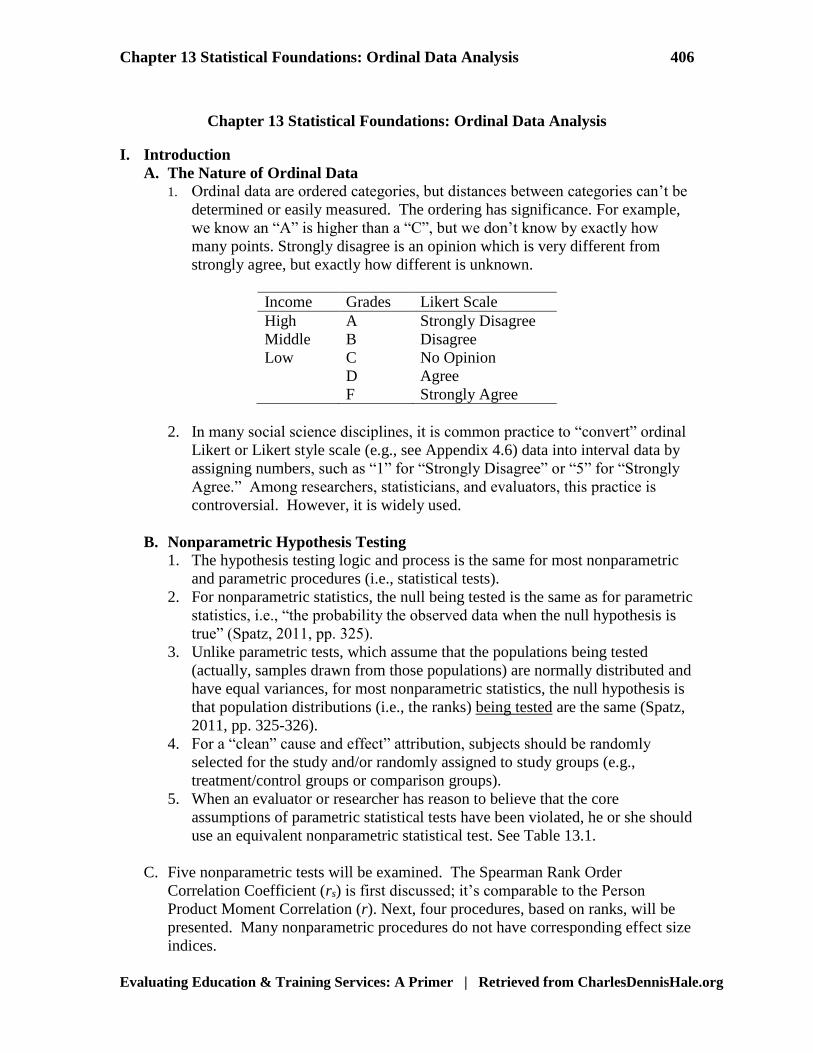
1. Ordinal data are ordered categories, but distances between categories can’t be

determined or easily measured. The ordering has significance. For example,

we know an “A” is higher than a “C”, but we don’t know by exactly how

many points. Strongly disagree is an opinion which is very different from

strongly agree, but exactly how different is unknown.

Income Grades Likert Scale

High A Strongly Disagree

Middle B Disagree

Low C No Opinion

D Agree

F Strongly Agree

2. In many social science disciplines, it is common practice to “convert” ordinal

Likert or Likert style scale (e.g., see Appendix 4.6) data into interval data by

assigning numbers, such as “1” for “Strongly Disagree” or “5” for “Strongly

Agree.” Among researchers, statisticians, and evaluators, this practice is

controversial. However, it is widely used.

B. Nonparametric Hypothesis Testing

1. The hypothesis testing logic and process is the same for most nonparametric

and parametric procedures (i.e., statistical tests).

2. For nonparametric statistics, the null being tested is the same as for parametric

statistics, i.e., “the probability the observed data when the null hypothesis is

true” (Spatz, 2011, pp. 325).

3. Unlike parametric tests, which assume that the populations being tested

(actually, samples drawn from those populations) are normally distributed and

have equal variances, for most nonparametric statistics, the null hypothesis is

that population distributions (i.e., the ranks) being tested are the same (Spatz,

2011, pp. 325-326).

4. For a “clean” cause and effect” attribution, subjects should be randomly

selected for the study and/or randomly assigned to study groups (e.g.,

treatment/control groups or comparison groups).

5. When an evaluator or researcher has reason to believe that the core

assumptions of parametric statistical tests have been violated, he or she should

use an equivalent nonparametric statistical test. See Table 13.1.

C. Five nonparametric tests will be examined. The Spearman Rank Order

Correlation Coefficient (rs) is first discussed; it’s comparable to the Person

Product Moment Correlation (r). Next, four procedures, based on ranks, will be

presented. Many nonparametric procedures do not have corresponding effect size

indices.



Table 13.1

Nonparametric Tests for Ordinal Data

Independent Variables Nonparametric Tests Parametric Tests

1, 2 Levels Wilcoxon Matched Pairs Dependent Samples t-test

1, 2 Levels Mann-Whitney U Test Independent Samples t-test

1, 3+ Levels Kruskal-Wallis 1 Way ANOVA 1 Way (Factor) AVOVA

2, 3+ Levels Friedman 2 Way ANOVA 1 Way Correlated ANOVA

II. Ordinal Data Analysis Statistical Tools

A. Spearman Rank Order Correlation Coefficient (rs)

1. The Spearman Rank Order procedure is applied when data are ordinal, i.e.,

ranked on a criterion, e.g., from least skillful to most skillful, poor to

excellent, etc. No “numbers” are used to represent the ordinal ranked

categories (Daniel, 1990, pp. 358-364). It is usually used when the number of

pairs is ≤ 20. Spatz (2011, pp. 342-345) discusses.

2. rs Characteristics:

a. Is a member of the Pearson family of procedures.

b. Ranges from -1.0 to +1.0

c. A high positive rs value indicates that the paired ranks are equal.

d. A high negative rs value indicates that the paired ranks are unequal.

e. A zero rs value indicates no relationship between the sets of ranks.

3. When the ranks are tied, i.e., two subjects are ranked equally, just average the

corresponding ranks.

a. Subjects “C” and “D” were ranked as equally skilled. In ranking these

two subjects, along with eight others, the places in the ranking (10-1)

would be averaged with the corresponding mean value assigned to both

“C” and “D”.

b. When the number of “ties” meet or exceed five and the number of subjects

exceeds ten, perform the PPMC procedure.

4. Case 13.1: Two senior trainers ranked 10 novice trainers by degree of

teaching skill, where 1 = the least skillful and 10 = the most skillful.

a. Computational Sequence

(1) Do the two senior trainers agree in their novice trainers ranking.

(2) State the hypothesis: Ho: rs = 0 or H1: rs ≠ 0

(3) Set alpha: ∂ = .05

(4) Select Test: Spearman Rank Order Correlation Coefficient

(5) Compute Test Statistic

(a) Construct Data Table

(b) Compute degrees of freedom (df = N) or 10, when N ≤ 16. When N

≥ 17. df = N-2.

(c) Substitute into Formula 13.1, The Spearman Rank Order

Correlation (Spatz, 2011, p. 343; Daniel, 1990, p. 359)



Table 13.2

Spearman Rank Order Case Data

Patient X’s Rank Y’s Rank D (x-y) D2

A 3 4 -1 1

B 2 1 1 1

C 5 6 -1 1

D 9 7 2 4

E 1 3 -2 4

F 10 10 0 0

G 8 9 -1 1

H 4 2 2 4

I 7 5 2 4

J 6 8 -2 4

N=10 ∑D = 0 ∑ D2 = 24

85.145.1)110(10

)24(61

)1(

61

22

2

NN

Drs

(6) Critical value = 0.648 at ∂ = .05 & df (or # of pairs) = 10 for a two-tail

test (Spatz, 2011, p. 404; Triola 1998, p. 725).

(7) Apply Decision Rules: Since rs = |.85| ≥ 0.648, we reject Ho: rs = 0, as

p < .05.

(8) There is a statistically significant relationship between the rankings.

The two senior trainers agreed on their rankings. We report rs = 0.85, p <

0.05.

(9) Effect Size Estimate: Applying Cohen’s (1988, pp. 79-80) effect size

criteria, since rs = |.85| indicates a large effect. We conclude that the

senior trainers strongly agreed in their ranking.

b. There is a “handy” Spearman rs critical value table at

<http://www.ace.upm.edu.my/~bas/5950/Spearman%20Rho%20Table.pdf

B. Wilcoxon Matched Pairs Signed Ranks “T” Test

1. The Wilcoxon Matched Pairs Test is the nonparametric equivalent to the

dependent samples t-test and is applied to ordinal data (Spatz, 2011, pp. 333-

338). Recall that there are three dependent designs: natural pairs (e.g. twins),

matched pairs, and repeated (before and after, like pretest and posttest).

Scores from the two groups must be logically paired.

2. The test statistic is “T.” The critical value is drawn from the critical values for

the Wilcoxon matched pairs signed rank T table. It is the differences that are



ranked not the values of the differences. The rank of “1” always goes to the

smallest difference.

3. A critical value table for the Wilcoxon Matched Pairs Sign Rank Test maybe

found at <http://facultyweb.berry.edu/vbissonnette/tables/wilcox_t.pdf>.

4. Computational Sequence (Case 13.2, Table 13.3)

a. For each pair of scores, find D, the difference between each pair.

Subtraction order is not important; we work with absolute value.

b. Rank each difference based on the absolute value of each. The rank of “1”

goes to the smallest difference; the rank of “2” goes to the next highest

difference and so on. Go from low to high, where the highest “D” has the

highest rank value.

(1) When one (1) “D” = zero (0.0), it is not assigned a rank; the

information is deleted from the computation; and N is reduced by one.

If two “D” values equal zero, then one is given a +1.5 ranking and the

second is given a -1.5 ranking. If three “D” values equal zero, then one

is dropped (reducing N by one) and the other two are assigned -1.5 and

+1.5 ranking.

(2) When “D” values are tied, the mean of the ranks which would have

been received is given to each of the tied ranks. See how pairs 5 and 6

are treated in Table 13.3.

c. To each value of D attach the sign of its difference, negative (-) or positive

(+) which is usually left off as it is understood. For Pair 1, D = -8, so the

value of its rank is negative. For Pair 3, D = 5, so its rank is positive.

d. Sum the positive and negative ranks separately. T is the absolute value of

the smaller of the two sums.

e. If the test statistic “T” is less than (<) the critical value “T”, the null

hypothesis is rejected. The same is true for the Mann-Whitney U Test.

f. Computation and Null Hypothesis Decision-Making

(1) Since the test statistic T = 11 is > the critical value T = 2, for a 2-tail

test where ∂ = 0.5, with 7 pairs (Spatz, 2011, p. 402; Triola 1998, p.

726), we retain the null hypothesis that there is no difference between

the rankings. We report T (7) = 11, p > 0.05.

(2) Remember that the dependent samples t-test could have been applied

to these Table 12.8 data but the decision was made to test the rankings

of the scores and not the scores themselves. In cases where there is

reason to believe that the populations are not normally distributed and

do not have equal score variances, one would use this test.

(3) The null hypothesis for the Wilcoxon Matched Pairs Test is that if the

populations are truly equal (i.e., there are no real differences), the

absolute values of the positive and negative sums will be equal and

any differences are due to sampling fluctuations.



Table 13.3

Wilcoxon Matched Pairs Test

Subject Variable A Variable B D Rank Signed Rank

1 18 26 -8 7 -7

2 16 19 -3 4 -4

3 25 20 5 5 5

4 25 24 1 1 1

5 24 22 2 1.5 1.5

6 23 21 2 1.5 1.5

7 25 18 7 6 6

Σ (+ ranks) = 15

Σ (- ranks) = -11

T = 11 (smallest absolute value)

5. Case 13.3: Eleven training assistants completed a teaching methods

workshop. Each was pre-tested before and post-tested after the workshop. A

Higher score on the tests indicates better teaching skills. When examining

dependent samples t-test assumptions, it was noted that the scores were not

normally distributed. So the scores were converted to ranks as found in Table

13.4.

a. Computational Sequence

(1) Did the workshop improve teaching skills? (2) d 0

(2) Ho: Population distributions are equal.

(3) H1: Population distributions are not equal.

(4) = 0.05 for a two-tail test

(5) Wilcoxon Matched Pairs Signed Ranks Test

(6) Compute the Test Statistic & Construct Data Table

Table 13.4

Teaching Workshop Case Data

Subject Pretest Posttest D Rank Signed Rank

A 10 14 -4 5 -5

B 11 19 -8 10 -9.5

C 9 13 -4 5 -5

D 11 12 -1 1 -1

E 14 22 -8 9 -9.5

F 6 11 -5 7 -7

G 13 17 -4 5 -5

H 12 18 -6 8 -8

I 19 19 0 Deleted Deleted

J 18 16 2 2 2

K 17 14 3 3 3



(a) Compute Number of Pairs N (#of pairs) - (# of deleted) or N = 10 (Subject I was deleted as there was no difference between pretest and posttest.)

(b) Compute the test statistic “T”

Σ (+ ranks) = 5

Σ (- ranks) = -50

T = 5 (smallest absolute value)

(c) Critical “T” Value: = 8 at ∂ = .05 in a 2-tail test with N = 10 pairs

(Spatz, 2011, p. 402; Triola 1998, p. 726)

(7) Apply Decision Rule: Since the test statistic of T = 5 is less than the

critical T value of T = 8, the null hypothesis is rejected.

(8) It appears that the workshop does improve teaching skills. We report T

(10) = 5, p < 0.05.

6. When the sample size is greater than 50, the T statistic is approximated using

the z-score and the SNC. Use Formula 13.2a, 13.2b and 13.2c (Spatz, 2011,

p. 337). First compute Formula13.2b and13.2c before Formula 13.2a.

a. Formula 13.2a Wilcoxon Matched Pairs Test N > 50

( ) T

T

T cz

Where: T = smaller sum of the signed ranks

c = 0.5, a correction factor

b. Formula 13.2b Wilcoxon Matched Pairs Test N > 50

( 1)

4T

N N

c. Formula 13.2c Wilcoxon Matched Pairs Test N > 50

( 1)(2 1)

24T

N N N

Where: N = number of pairs for N1 and N2.

d. Decision Rules

(1) For a 2-tail test, reject the null hypothesis (Ho) if the computed test

statistic “z” falls outside the interval -1.96 and +1.96 at ∂ = .05.




statistic “z” falls outside the interval -2.58 and +2.58 at ∂ = .01.

C. The Mann-Whitney U Test

1. The Mann-Whitney U Test is the nonparametric equivalent to the independent

samples t-test.

a. The Mann-Whitney test produces the U statistic which is based upon the U

distribution (Spatz, 2011, pp. 327-333). Distributions for small samples

(N1 ≤ 20 & N2 ≤ 20), the distribution’s shape depends on the sample size.

b. To detect errors, the two U value sums in the Mann-Whitney U Test

equals the product of (N1)(N2), i.e., (N1) multiplied by (N2).

c. In the Mann-Whitney U Test, it makes no difference whether the highest

or lowest score (should you have to rank scores) is given the rank of 1.

d. Most researchers using the Mann-Whitney test assume that the two

distributions has the same form (shape) but most likely differ in central

tendency.

(1) A significant “U” is typically attributed to a difference in central

tendency between the two groups; “U” actually compares

distributions.

(2) The smaller the U value, the more different the two groups are.

e. Ties between ranks are handled in the same manner as in the Wilcoxon

Matched Pairs Signed Ranks test. If the ties are in the same group, then the

U value is not affected. If there are several ties across both groups, the

correction suggested by Kirk (2008, p. 504) should be applied.

f. A Mann-Whitney U Test critical value table is located at

<http://www.alamo.edu/sac/media/puentes/Documentation/CriticalValues

U.pdf>.

2. Computational Process for Small Sample

a. Formula 13.3a The Mann-Whitney U Test Small Sample for R1 (Spatz,

2011, p. 327)

1 1

1 2 1

( 1)( )( )

2

N NU N N R

Where N1 = Number comprising group one

N2 = Number comprising group two

ΣR1 = sum of ranks for group one

b. Formula 13.3b The Mann-Whitney U Test Small Sample for R2 (Spatz,

2011, p. 328)

2 2

1 2 2

( 1)( )( )

2

N NU N N R

Where N1 = Number comprising group one

N2 = Number comprising group two

Σ R2 = Sum of ranks for group two



3. Case 13.4: Eleven freshmen students were collectively ranked by a team of

three professors as to their academic competence. Unknown to the professors,

some freshman had completed an academic competence course where they

were exposed to study habits, time management, academic culture, and

managing for productive academic relationships.

(a) Computational Sequence

(1) Does the freshman workshop improve academic competence? (2) d 0

(2) Ho: Population distributions are equal.

(3) H1: Population distributions are not equal.

(4) = 0.05 for a two-tail test

(5) Mann-Whitney U Test

(6) Compute the Test Statistic

(a) Construct Data Table:

Table 13.5

Academic Competence Case Data

Student Mean Ranking Take Course

A 4 N0

B 9 Yes

C 7 Yes

D 6 No

E 5 Yes

F 3 No

G 2 Yes

H 10 Yes

I 11 Yes

J 1 No

K 8 No

(b) Determine N’s: N1 = 5 (No, Course) N2 = 6 (Yes, Course)

(c) Compute the test statistic “U”

ΣR1 (yes) = 22

ΣR2 (no) = 44

U = 7 (smallest absolute value)

[1] Apply Formula 13.3a for the “No” group (R1)

1 1

1 2 1

( 1) 5(5 1)( )( ) (5)(6) 22

2 2

N NU N N R



30

30 22 45 22 232

U

[2] Apply Formula 13.3b for the “Yes” group (R2)

2 2

1 2 2

( 1) 6(6 1)( )( ) (5)(6) 44

2 2

N NU N N R

42

30 44 30 21 44 72

U

(d) Critical “U” Value: = 3 at ∂ = .05 in a 2-tail test at the intersection

of column N1 = 5 and row N2 = 6 in the Mann-Whitney Critical

Value Table (Spatz, 2011, p. 401). A critical value table (2-tail

test) is found at

<http://www.lesn.appstate.edu/olson/stat_directory/Statistical%20p

rocedures/Mann_Whitney%20U%20Test/Mann-

Whitney%20Table.pdf>

(7) Apply Decision Rule: Since the test statistic of U = 7 (the smaller of

R1 or R2) is greater than the critical U value of U = 3, the null

hypothesis is retained. (Remember, to reject H0, the critical U must be equal to

or less than the critical value shown in the table.)

(8) It appears that the workshop does not improve academic competency

as the distributions of the two groups are statistically equal. We report

U (5, 6) = 7, p > 0.05.

(9) Effect Size Estimation: Redfern (2011) offers the Probability of

Superiority (PS) as an effect size indices. Formula 13.3c is

1 2

7 70.233

5 6 30

UPS

n n

Redfern provides interpretive guidance. No effect means PS = 0.50.

The greater distance PS is from 0.50, the greater the effect. Unlike the

correlation coefficient, there aren’t qualitative labels to place on a PS

value, such as small medium or large. The interpretation must be

within the context of the study and/or the comparison of the study’s PS

to other similar studies. So, given the context of Case 13.4, it would

appear that the preparation course for the incoming freshman made a

positive difference, comparing the mean rank for the “No Course”

students ( 4.4X ) and the “Yes Course” students ( 7.3X ).

Remember, the smaller the U value, the more different the two groups

are.

4. When the sample size is greater than 21, in either N1 or N2, the U test statistic

is approximated using the z-test and the SNC. The Mann-Whitney U Test for

N1 or N2, > 21 (Spatz, 2011, pp. 330-332) is used. To use Formula 13.4a, you



must calculate Formula 13.3a and 13.3b to identify the smaller U value. Spatz

(2011, p. 331) provides a computational example.

a. Formula 13.4a (Spatz, 2011, p. 330).

( )

U

U

U cz

Where: U is the smaller of the two U values

“c” is a 0.05 correction factor

b. Formula 13.4b

1 2( )( )

2U

N N

c. Formula 13.4c

1 2 1 2( )( )( 1)

12U

N N N N

Where: U

= N= # of pairs for N1 and N2

d. Decision Rules (Spatz, 2011, p. 330)


statistic “z” ≥ |1.96| at ∂ = .05.


statistic “z” ≥ |2.58| at ∂ = .01.


statistic “z” ≥ 1.65 at ∂ = .05.


statistic “z” ≥ 2.33 at ∂ = .01.

E. Kruskal-Wallis One Way ANOVA

1. Introduction (Sprent & Smeeton, 2001, pp. 199-203)

a. Applies to one independent variable with 3 or more levels

b. Can be applied to ranked data (ordinal), means, or medians. Remember a

shift in mean or median reflects an additive treatment effect.

c. The null hypothesis (H0) is that the group or sample ranks, means, or

medians are from the same population, i.e., there are no differences.

d. The alternative hypothesis (H1) is that there is a difference among ranks,

means, or medians.

e. For ranks assign “1” to the lowest rank; “2” to the next lowest; etc. When

there are at least “5” ranks in each level, the Chi Square Critical Value

Table can be used to assess statistical significance (Lowry, 2011a). f. Degrees of Freedom (df): k-1, where k = 3 of samples or independent variable

levels; so, there would be 2 degrees of freedom.

g. Sprent & Smeeton (2001, pp. 199-2003) refer to the test statistic as “T,” so

shall we; however, many others (Daniel, 1990; Siegel, 1956) refer to the

test statistic as “H.”



h. The Kruskal-Wallis test can be an alternative to an unbalanced (different

subject numbers in independent variable levels) to a parametric One Way

ANOVA (Lowery, 2011a).

i. The Kruskal-Wallis test is an omnibus test in that it will identify whether

or not there are statistically significant differences between been rankings,

but will not tell us which pairs of ranks are different.

(1) A post hoc pair-wise comparison test (Dunn’s Test) is available; it’s

laborious and tedious to compute with a calculator, thus making

computational errors more likely. One might calculate a Mann-

Whitney U test for each pair-wise comparison with a Bonferroni

adjustment (see p. 487).

(2) In the absence of a statistical processing program (e.g., SAS or SPSS),

some rely on logical analysis by examining rank sums or rank means

or medians as in Table 13.6 or 13.7. Such conclusion drawing may

prove inaccurate.

(3) Effect size computation for the Kruskal-Wallis test is not straight

forward.

2. Kruskal-Wallis without Ties

a. Case 13.5: Trainees were assigned randomly to three separate training

methodologies: eLearning (A), Direct Instruction (B), and Self-study (C).

At the end of the training course a criterion referenced examination was

given, with a point scale ranging from “0” to “100.” The highest possible

score was 100 points.

b. Computation Sequence

(1) The null hypothesis (H0) is that there are no differences between the

rankings among the 3 groups. The alternative hypothesis (H1) is that

the ranks among the 3 groups differ.

(2) After ranking the data, Data Table 13.6 emerges.

(3) Apply the Kruskal-Wallis One Way ANOVA at ∂ = 0.05.

(4) Compute the test statistic, using Formula 13.5 (Sprent & Smeeton,

2001, pp. 199).

12 (12)(1458.50)

3( 1) 3(16 1) 64.346 51.11 13.236( 1) (16)(17)

kS

T NN N

2 2 2 2(81) (40) (15)

( ) 1458.506 5 5

ik i

i

sS

n

(5) Using the Chi-Square Critical value table (Spatz, 2011, p. 393), we

find the critical value to be 5.991, at 2 df (k-1=3-1=2) and alpha (∂) =

0.05. Since the test statistic T = 13.236 >5.991, we reject the null

hypothesis (H0) stating there is no differences between ranks, T (2) =

13.236, p < 0.05.



(6) By examining rank means (Table 13.6), training approach did appear

to influence score ranking, and by extension, trainee performance. But

without a post-hoc comparison test, we can’t be absolutely sure.

Table 13.6

Data Table

Score Rank Method

96 16 A

93 15 A

91 14 A

89 13 A

87 12 A

85 11 A

83 10 B

82 9 B

80 8 B

79 7 B

75 6 B

74 5 C

72 4 C

70 3 C

68 2 C

66 1 C

∑A=81 ∑B=40 ∑C=15

13.5A

X 8B

X 3C

X

3. Kruskal-Wallis with Ties

a. Case 13.6: A large multi-national corporation was conducting a “Train the

Trainer” workshop. Twenty trainees were randomly assigned to one of

three senior trainers. After the course, Trainees were assigned a sample

lesson and were ranked on instructional performance scale, using a 50

point scale (1, lowest to 50, highest), by the associate training manager. As

the training manager, you want to determine the most effective senior

trainer, A, B, or C.






(3) Apply the Kruskal-Wallis One Way ANOVA at ∂ = 0.05.


2001, pp. 201).

( 1)( ) (19)(2338.08 2205) (19)(133.08) 2528.52

3.8022870 2205 665 665

k

r

N S CT

S C

( 1)(2 1) 20(21)(41) 17,220

2,8706 6 6

r

N N NS



2 21( ) ( 1) (.25) 20(21) (.25) (20)(441) (.25)(88520) 2,2054

C N N

Table 13.7

Data Table

Score

Rank

Adjusted

Rank

Trainer

48 20 20 C

46 19 19 C

42 18 18 C

40 17 17 B

38 16 16 A

36a 15 14 C

36a 14 14 A

36a 13 14 B

35 12 12 C

32 11 11 B

31 10 10 A

30 9 9 C

28 8 8 A

27 7 7 B

26b 6 5.5 C

26b 5 5.5 A

25 4 4 B

23 3 3 A

22 2 2 B

20 1 1 B

∑A=56.5 ∑B=56 ∑C=97.5 ∑=210 a Give the mid-point of the three ranking as

the “adjusted rank.” b Give the average of the two ranks as the

“adjusted rank.”

(5) Using the Chi-Square Critical value table (Spatz, 2011, p. 393), we

find the critical value to be 5.991, at 2 df (k-1or 3-1=2) and alpha (∂) =

0.05. Since the test statistic T = 3.802 < 5.991, we retain the null

hypothesis (H0) stating there is no differences between ranks, T (2) =

3.802, p > 0.05.

(6) It appears the senior trainers are equally effective.

F. Friedman Two Way ANOVA for Related Samples

1. Introduction (Daniel, 1990; Sprent & Smeeton, 2001)

a. Friedman’s Two Way ANOVA is the nonparametric analogue to the 1

Way Correlated or Repeated ANOVA.

b. The rationale is that subject groups, called blocks, have the same median

and that any difference in block medians is due to the application of at

least one of the independent variables (AKA Treatments).

(1) The null hypothesis is0 1 2 3

:j

H x x x x .



(2) The null hypothesis is1 1 2 3:

jH x x x x .

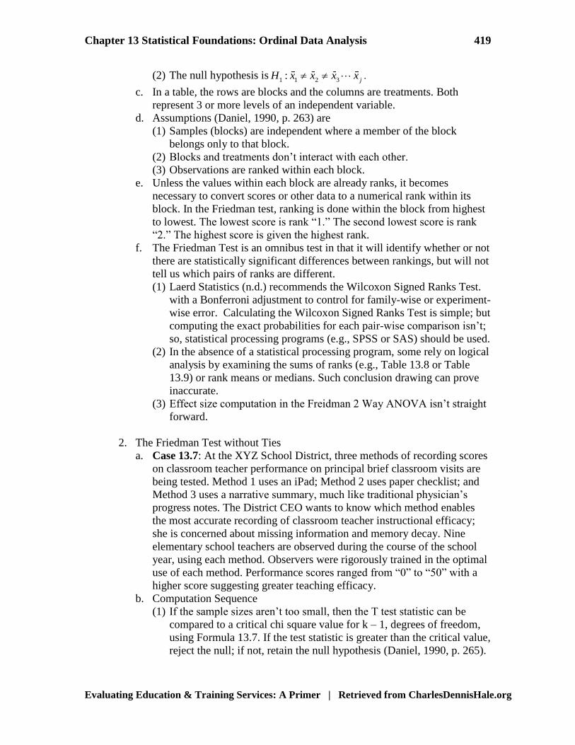
c. In a table, the rows are blocks and the columns are treatments. Both

represent 3 or more levels of an independent variable.

d. Assumptions (Daniel, 1990, p. 263) are

(1) Samples (blocks) are independent where a member of the block

belongs only to that block.

(2) Blocks and treatments don’t interact with each other.

(3) Observations are ranked within each block.

e. Unless the values within each block are already ranks, it becomes

necessary to convert scores or other data to a numerical rank within its

block. In the Friedman test, ranking is done within the block from highest

to lowest. The lowest score is rank “1.” The second lowest score is rank

“2.” The highest score is given the highest rank.

f. The Friedman Test is an omnibus test in that it will identify whether or not

there are statistically significant differences between rankings, but will not

tell us which pairs of ranks are different.

(1) Laerd Statistics (n.d.) recommends the Wilcoxon Signed Ranks Test.

with a Bonferroni adjustment to control for family-wise or experiment-

wise error. Calculating the Wilcoxon Signed Ranks Test is simple; but

computing the exact probabilities for each pair-wise comparison isn’t;

so, statistical processing programs (e.g., SPSS or SAS) should be used.

(2) In the absence of a statistical processing program, some rely on logical

analysis by examining the sums of ranks (e.g., Table 13.8 or Table

13.9) or rank means or medians. Such conclusion drawing can prove

inaccurate.

(3) Effect size computation in the Freidman 2 Way ANOVA isn’t straight

forward.

2. The Friedman Test without Ties

a. Case 13.7: At the XYZ School District, three methods of recording scores

on classroom teacher performance on principal brief classroom visits are

being tested. Method 1 uses an iPad; Method 2 uses paper checklist; and

Method 3 uses a narrative summary, much like traditional physician’s

progress notes. The District CEO wants to know which method enables

the most accurate recording of classroom teacher instructional efficacy;

she is concerned about missing information and memory decay. Nine

elementary school teachers are observed during the course of the school

year, using each method. Observers were rigorously trained in the optimal

use of each method. Performance scores ranged from “0” to “50” with a

higher score suggesting greater teaching efficacy.


(1) If the sample sizes aren’t too small, then the T test statistic can be

compared to a critical chi square value for k – 1, degrees of freedom,

using Formula 13.7. If the test statistic is greater than the critical value,

reject the null; if not, retain the null hypothesis (Daniel, 1990, p. 265).







(4) Apply Friedman Test at ∂ = 0.05.


2001, pp. 214).

(6) Using the Chi-Square Critical value table (Spatz, 2011, p. 393), when

using Formula 13.7, we find the critical value to be 5.991, at 2 df (k-

1or 3-1=2) and alpha (∂) = 0.05. Since the test statistic T = 2.89 <

5.991, we retain the null hypothesis (H0) stating there is no differences

between ranks, T (2) = 3.802, p > 0.05.

Table 13.8

Friedman Test without Ties Data Table

Teacher

Method 1 Method 2 Method 3

Score Rank Score Rank Score Rank

A 42 3 39 2 33 1

B 44 3 30 1 40 2

C 36 2 38 3 29 1

D 32 2 37 3 26 1

E 41 2 38 1 45 3

F 46 3 39 1 40 2

G 40 3 27 1 31 2

H 41 3 25 1 31 2

I 26 1 29 2 32 3

∑R1 = 22 ∑R2 = 15 ∑R3 = 17

Formula 13.7

2 2 2 2

12 12[(22) (15) (17) ]3 ( 1) (3)(9)(3 1)

( 1) (9)(3)(3 1)

i is

T b tbt t

(12)(998)

108 110.888 108 2.89108

Where: b = number of blocks (e.g., rated teachers)

t = number of treatments

3. The Freidman Test with Ties

a. Case 13.8: Same as Table 13.8; but with 2 additional teachers and

reordered ranks.








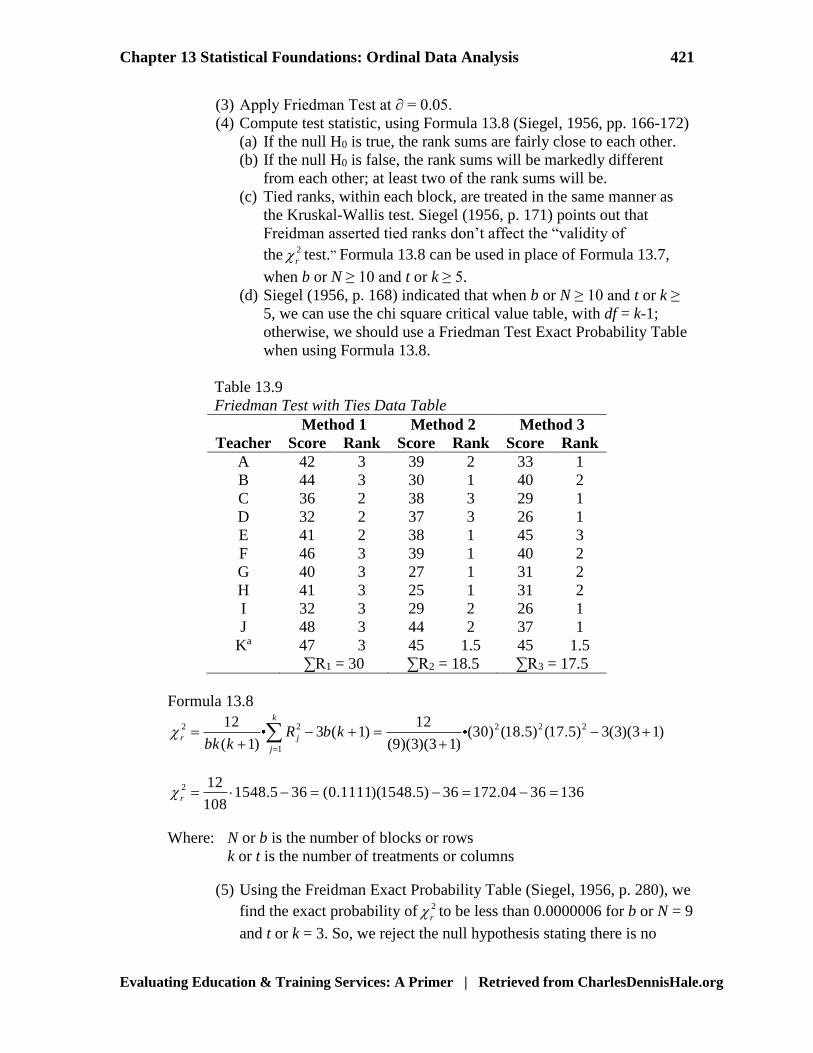
(3) Apply Friedman Test at ∂ = 0.05.

(4) Compute test statistic, using Formula 13.8 (Siegel, 1956, pp. 166-172)

(a) If the null H0 is true, the rank sums are fairly close to each other.

(b) If the null H0 is false, the rank sums will be markedly different

from each other; at least two of the rank sums will be.

(c) Tied ranks, within each block, are treated in the same manner as

the Kruskal-Wallis test. Siegel (1956, p. 171) points out that

Freidman asserted tied ranks don’t affect the “validity of

the 2

r test.” Formula 13.8 can be used in place of Formula 13.7,

when b or N ≥ 10 and t or k ≥ 5.

(d) Siegel (1956, p. 168) indicated that when b or N ≥ 10 and t or k ≥

5, we can use the chi square critical value table, with df = k-1;

otherwise, we should use a Friedman Test Exact Probability Table

when using Formula 13.8.

Table 13.9

Friedman Test with Ties Data Table

Teacher

Method 1 Method 2 Method 3

Score Rank Score Rank Score Rank

A 42 3 39 2 33 1

B 44 3 30 1 40 2

C 36 2 38 3 29 1

D 32 2 37 3 26 1

E 41 2 38 1 45 3

F 46 3 39 1 40 2

G 40 3 27 1 31 2

H 41 3 25 1 31 2

I 32 3 29 2 26 1

J 48 3 44 2 37 1

Ka 47 3 45 1.5 45 1.5

∑R1 = 30 ∑R2 = 18.5 ∑R3 = 17.5

Formula 13.8

2 2 2 2 2

1

12 123 ( 1) (30) (18.5) (17.5) 3(3)(3 1)

( 1) (9)(3)(3 1)

k

r j

j

R b kbk k

2 12

1548.5 36 (0.1111)(1548.5) 36 172.04 36 136108

r

Where: N or b is the number of blocks or rows

k or t is the number of treatments or columns

(5) Using the Freidman Exact Probability Table (Siegel, 1956, p. 280), we

find the exact probability of 2

r to be less than 0.0000006 for b or N = 9

and t or k = 3. So, we reject the null hypothesis stating there is no



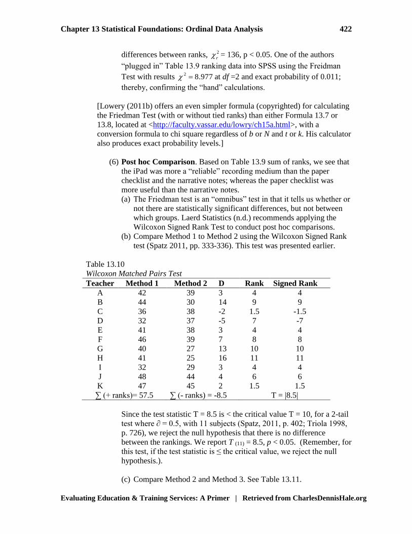
differences between ranks, 2

r = 136, p < 0.05. One of the authors

“plugged in” Table 13.9 ranking data into SPSS using the Freidman

Test with results 28.977 at df =2 and exact probability of 0.011;

thereby, confirming the “hand” calculations.

[Lowery (2011b) offers an even simpler formula (copyrighted) for calculating

the Friedman Test (with or without tied ranks) than either Formula 13.7 or

13.8, located at <http://faculty.vassar.edu/lowry/ch15a.html>, with a

conversion formula to chi square regardless of b or N and t or k. His calculator

also produces exact probability levels.]

(6) Post hoc Comparison. Based on Table 13.9 sum of ranks, we see that

the iPad was more a “reliable” recording medium than the paper

checklist and the narrative notes; whereas the paper checklist was

more useful than the narrative notes.

(a) The Friedman test is an “omnibus” test in that it tells us whether or

not there are statistically significant differences, but not between

which groups. Laerd Statistics (n.d.) recommends applying the

Wilcoxon Signed Rank Test to conduct post hoc comparisons.

(b) Compare Method 1 to Method 2 using the Wilcoxon Signed Rank

test (Spatz 2011, pp. 333-336). This test was presented earlier.

Table 13.10


Teacher Method 1 Method 2 D Rank Signed Rank

A 42 39 3 4 4

B 44 30 14 9 9

C 36 38 -2 1.5 -1.5

D 32 37 -5 7 -7

E 41 38 3 4 4

F 46 39 7 8 8

G 40 27 13 10 10

H 41 25 16 11 11

I 32 29 3 4 4

J 48 44 4 6 6

K 47 45 2 1.5 1.5

∑ (+ ranks)= 57.5 ∑ (- ranks) = -8.5 T = |8.5|

Since the test statistic T = 8.5 is < the critical value T = 10, for a 2-tail

test where ∂ = 0.5, with 11 subjects (Spatz, 2011, p. 402; Triola 1998,

p. 726), we reject the null hypothesis that there is no difference

between the rankings. We report T (11) = 8.5, p < 0.05. (Remember, for

this test, if the test statistic is ≤ the critical value, we reject the null

hypothesis.).

(c) Compare Method 2 and Method 3. See Table 13.11.

http://faculty.vassar.edu/lowry/ch15a.html



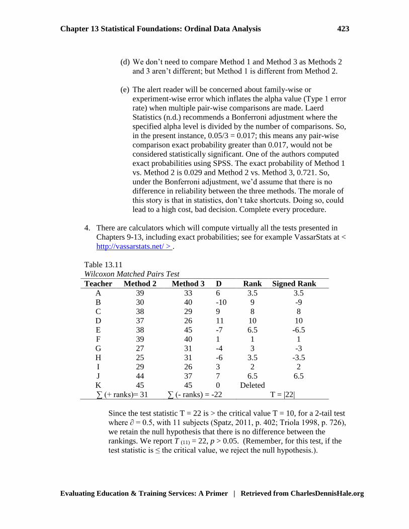
(d) We don’t need to compare Method 1 and Method 3 as Methods 2

and 3 aren’t different; but Method 1 is different from Method 2.

(e) The alert reader will be concerned about family-wise or

experiment-wise error which inflates the alpha value (Type 1 error

rate) when multiple pair-wise comparisons are made. Laerd

Statistics (n.d.) recommends a Bonferroni adjustment where the

specified alpha level is divided by the number of comparisons. So,

in the present instance, 0.05/3 = 0.017; this means any pair-wise

comparison exact probability greater than 0.017, would not be

considered statistically significant. One of the authors computed

exact probabilities using SPSS. The exact probability of Method 1

vs. Method 2 is 0.029 and Method 2 vs. Method 3, 0.721. So,

under the Bonferroni adjustment, we’d assume that there is no

difference in reliability between the three methods. The morale of

this story is that in statistics, don’t take shortcuts. Doing so, could

lead to a high cost, bad decision. Complete every procedure.

4. There are calculators which will compute virtually all the tests presented in

Chapters 9-13, including exact probabilities; see for example VassarStats at <

http://vassarstats.net/ > .

Table 13.11


Teacher Method 2 Method 3 D Rank Signed Rank

A 39 33 6 3.5 3.5

B 30 40 -10 9 -9

C 38 29 9 8 8

D 37 26 11 10 10

E 38 45 -7 6.5 -6.5

F 39 40 1 1 1

G 27 31 -4 3 -3

H 25 31 -6 3.5 -3.5

I 29 26 3 2 2

J 44 37 7 6.5 6.5

K 45 45 0 Deleted

∑ (+ ranks)= 31 ∑ (- ranks) = -22 T = |22|

Since the test statistic T = 22 is > the critical value T = 10, for a 2-tail test

where ∂ = 0.5, with 11 subjects (Spatz, 2011, p. 402; Triola 1998, p. 726),

we retain the null hypothesis that there is no difference between the

rankings. We report T (11) = 22, p > 0.05. (Remember, for this test, if the

test statistic is ≤ the critical value, we reject the null hypothesis.).

http://faculty.vassar.edu/lowry/VassarStats.html%3e

http://faculty.vassar.edu/lowry/VassarStats.html%3e



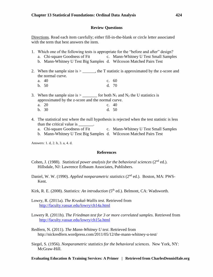
Review Questions

Directions. Read each item carefully; either fill-in-the-blank or circle letter associated

with the term that best answers the item.

1. Which one of the following tests is appropriate for the “before and after” design?

a. Chi-square Goodness of Fit c. Mann-Whitney U Test Small Samples

b. Mann-Whitney U Test Big Samples d. Wilcoxon Matched Pairs Test

2. When the sample size is > ______, the T statistic is approximated by the z-score and

the normal curve.

a. 40 c. 60

b. 50 d. 70

3. When the sample size is > _______ for both N1 and N2 the U statistics is

approximated by the z-score and the normal curve.

a. 20 c. 40

b. 30 d. 50

4. The statistical test where the null hypothesis is rejected when the test statistic is less

than the critical value is _______.

a. Chi-square Goodness of Fit c. Mann-Whitney U Test Small Samples

b. Mann-Whitney U Test Big Samples d. Wilcoxon Matched Pairs Test

Answers: 1. d, 2. b, 3. a, 4. d.

References

Cohen, J. (1988). Statistical power analysis for the behavioral sciences (2nd ed.).

Hillsdale, NJ: Lawrence Erlbaum Associates, Publishers.

Daniel, W. W. (1990). Applied nonparametric statistics (2nd ed.). Boston, MA: PWS-

Kent.

Kirk, R. E. (2008). Statistics: An introduction (5th ed.). Belmont, CA: Wadsworth.

Lowry, R. (2011a). The Kruskal-Wallis test. Retrieved from


Lowery R. (2011b). The Friedman test for 3 or more correlated samples. Retrieved from


Redfern, N. (2011). The Mann-Whitney U test. Retrieved from

http://nickredfern.wordpress.com/2011/05/12/the-mann-whitney-u-test/

Siegel, S. (1956). Nonparametric statistics for the behavioral sciences. New York, NY:

McGraw-Hill.





Spatz, C. (2011). Basic statistics: Tales of distributions (10th ed.). Belmont, CA:

Wadsworth.

Sprent, P. & Smeeton, N. C. (2001). Applied nonparametric statistical methods (3rd ed.).

New York, NY: Chapman & Hall/CRC

Triola, M. F. (1998). Elementary statistics (7th ed.) Reading, MA: Addison-Wesley.

Documents

Unit 20 Analysis of Nominal Data - Charles Dennis Halecharlesdennishale.org/Evaluating-Education-and-Training-Services/... · Likert or Likert style scale ... information is deleted