Urban Stormwater BMP Performance Monitoring - … · Urban Stormwater BMP Performance Monitoring ... National Stormwater Best Management Practices Database, ... Engineering Hydrology

Urban Stormwater BMP Performance Monitoring A Guidance Manual for Meeting the National Stormwater BMP Database Requirements

208 April 25, 2002

References American Society for Testing and Materials. 1995. Standard Guide for Selection of Weirs and Flumes for Open-Channel Flow Measurement of Water (D5640). American Society for Testing and Materials, West Conshohocken, PA. American Society for Testing and Materials. 1997. Standard Guide For Monitoring Sediment in Watersheds. ASTM D 6145-97. American Society for Testing and Materials. 2000. Standard Test Method for Determining Sediment Concentration in Water Samples. ASTM Designation D 3977-97, 395- 400. ASCE. 1999. National Stormwater Best Management Practices Database, Verision 1. American Society of Civil Engineers, Urban Water Resource Research Council, June. ASCE. 2000. Data Evaluation Report, Task 3.4. National Stormwater Best Management

Practices Database Project. June. Burton, A.G. and R. Pitt. 2001. Stomwater Effects Handbook: A Toolbox for Watershed

Managers, Scientists, and Engineers. Lewis Publishers, Boca Raton, FL. Caltrans. 1997. Guidance Manual: Stormwater Monitoring Protocols. Prepared by Larry

Walker and Associates and Woodward-Clyde Consultants. August 15. Caltrans. 2000. California Department of Transportation District 7 Litter Management

Pilot Study, Final Report, Caltrans Document No. CT-SW-RT-00-013, June 26.

Cave, K. A., and L.A. Roesner. 1994. Overview of Stormwater Monitoring Needs. Proceedings of the Engineering Foundation Conference on Stormwater Monitoring. August 7-12, Crested Butte, CO. Chow, V.T. 1954. The lognormal distribution and its engineering applications. Proc., American Society of Civil Engineers. 110, 607-628. Chow, V.T. 1959. Open-Channel Hydraulics. McGraw-Hill, New York, NY. Coffey, S.W., and M.D. Smolen. 1990. The Nonpoint Source Manager's Guide to Water Quality Monitoring - Draft. Developed under EPA Grant Number T-9010662. U.S. Environmental Protection Agency, Water Management Division, Region 7, Kansas City, MO. Cochran, W.G. 1963. Sampling Techniques. Second Edition. John Wiley and Sons, Inc.

New York, New York.


209 April 25, 2002

Driscoll, E., G. Palhegyi, E. Strecker, and P. Shelley. 1989. Analysis of Storm Event Characteristics for Selected Rainfall Gauges Throughout the United States. Draft Rep. Prepared for U.S. Environmental Protection Agency, Woodward-Clyde Consultants, Oakland, CA. Driscoll, E.D., P.E. Shelly, and E.W. Strecker. 1990. Pollutant Loadings and Impacts from

Stormwater Runoff, Volume III: Analytical Investigation and Research Report. Federal Highway Administration Final Report FHWA-RD-88-008, 160 p.

EPA. 1983. Results of the Nationwide Urban Runoff Program, volume I – Final Report.

U.S. Environmental Protection Agency, Water Planning Division, Washington D.C.

EPA. 1989. Analysis of Storm Event Characteristics for Selected Gages throughout the

United States. Environmental Protection Agency. Washington D.C. EPA. 1993a. Guidance Specifying Management Measures for Sources of Nonpoint

Pollution in Coastal Waters. EPA-840-B-93- 001c. U.S. Environmental Protection Agency, Office of Water, Washington D.C.

EPA. 1993b. Investigation of Inappropriate Entries into Storm Drainage Systems: A

User’s Guide. EPA-600-R-92-238. U.S. Environmental Protection Agency, Office of Research and Development, Washington D.C.

EPA, 1993c. Memo. Office of Water Policy and Technology. Guidance on Interpretation

and Implementation of Aquatic Life Metals Criteria, Washington, D.C. EPA. 1994a. Laboratory Data Validation: Functional Guidelines for Evaluating

Inorganics Analyses. U.S. Environmental Protection Agency, Data Review Workgroup, Washington, D.C.

EPA. 1994b. Laboratory Data Validation: Functional Guidelines for Evaluating

Organics Analyses. U.S. Environmental Protection Agency, Data Review Workgroup, Washington, D.C.

EPA. 1994c. Guidance for the Data Quality Objectives Process. EPA-QA/G-4. U.S.

Environmental Protection Agency. EPA. 1997. Monitoring Guidance for Determining the Effectiveness of Nonpoint Source

Controls. EPA 841-B-96-004. U.S. Environmental Protection Agency, Office of Water, Washington, D.C. September.

FHWA. 2000. Stormwater Best Management Practices in an Ultra-Urban Setting:

Selection and Monitoring. FHWA-EP-00-002. U.S. Department of Transportation. Federal Highway Administration. Washington, D.C., May.


210 April 25, 2002

FHWA. 2000. Guidance Manual for Monitoring Highway Runoff Water Quality.

Federal Highway Administration, U.S. Department of Transportation. Federal Highway Administration. Washington, D.C.

Fischer, H. B., List, J. E., KOH, R. C. Y., Imberger, J., and N.H. Brooks. 1979. Mixing in

Inland and Coastal Waters. Academic Press Inc., San Diego, CA. Gilbert, R.O. 1987. Statistical Methods for Environmental Pollution Monitoring. John

Wiley and Sons, Inc. New York, New York. Grant, D.M. and B.D. Dawson. 1997. ISCO Open Channel Flow Measurement Handbook. ISCO Environmental Division. Lincoln, NE. Gray, J.R., G.D. Glysson, and L.M. Turcios. 2000. Comparability and reliability of total suspended solids and suspended-sediment concentration data. U.S. Geological Survey Water-Resources Investigations Report 00-4191. U.S. Geological Survey. Green, D., T. Grizzard, and C. Randall. 1994. Monitoring of Wetlands, Wet Ponds, and Grassed Swales. In Proceedings of the Engineering Foundation Conference on Storm Water Monitoring. August 7-12, Crested Butte, CO. Gupta, R.S. 1989. Hydrology and Hydraulic Systems. Prentice Hall. NJ. Gwinn, W.R., and D.A. Parsons. 1976. Discharge Equations for HS, H and HL Flumes. Journal of the Hydraulics Division American Society of Civil Engineers, Vol. 102, No. HY1 pp. 73-89. Harremoes, P. 1988. Stochastic models for estimations of extreme pollution from urban runoff. Water Resource Bulletin, 22, 1017-1026. Harrison, D. 1994. Policy and Institutional Issues of NPDES Monitoring: Local Municipal Perspectives of Stormwater Monitoring. Proceedings of the Engineering Foundation Conference on Storm Water Monitoring. August 7-12, Crested Butte, CO.

James, W. 2001. http://131.104.80.10/webfiles/james/KeyModels.html.

Loftis, J.C., L.H. MacDonald, S. Streett, H.K. Iyer, and K. Bunte. 2001. Detecting Cumulative Watershed Effects: The Power of Pairing. In Review Journal of Hydrology.

Martin, E.H., and J.L. Smoot. 1986. Constituent-load changes in urban storm water runoff routed through a detention pond-wetland system in central Florida. Water Resources Investigation Report 85-4310. U.S. Geological Survey.

http://131.104.80.10/webfiles/james/KeyModels.html.


211 April 25, 2002

Martin, G.R., J.L. Smoot, and K.D. White. 1992. A Comparison of Surface-Grab and Cross Sectionally Integrated Stream-Water-Quality Sampling Methods. Water Environment Research. November/December 1992. Minton, G.R. 1998. Stormwater Treatment Northwest, Vol. 4, No. 3, August. National Urban Runoff Program. 1983. Final Report. U.S. Environmental Protection Agency Water Planning Division, Washington, D.C. Oswald, G.E., and R. Mattison. 1994. Protocols for Monitoring the Effectiveness of Structural Stormwater Treatment Devices. In Proceedings of the Engineering Foundation Conference on Storm Water Monitoring. August 7-12, Crested Butte, CO. Pitt, R. 1979. Demonstration of Nonpoint Pollution Abatement Through Improved Street

Cleaning Practices, EPA-600/2-79-161, U.S. Environmental Protection Agency, Cincinnati, Ohio.

Pitt, R. 2001. Personal Correspondence. Peer review meeting, August. Pitt, R. and K. Parmer. 1995. Quality Assurance Project Plan (QAPP) for EPA

Sponsored Study on Control of Stormwater Toxicants. Department of Civil and Environmental Engineering, University of Alabama at Birmingham.

Ponce, V.M. 1989. Engineering Hydrology Principles and Practices. Prentice Hall, Englewood Cliffs, NJ. Ruthven, D.M. 1971. "The Dispersion of a Decaying Effluent Discharged Continuously

into a Uniformly Flowing Stream," Water Research, 5(6) 343-352. Quigley, M.M, and E.W. Strecker. 2000. Protocols and methods for evaluating the performance of stormwater source controls. NATO Advanced Research Workshop on Source Control Measures for Stormwater Runoff, St. Marienthal, Ostritz, Germany. Saunders, T.G. 1983. Design of Networks for Monitoring Water Quality. Water

Resources Publications. December. Schueler, T.R. 1987. Controlling Urban Runoff: A Practical Manual for Planning and Designing Urban BMPs. Washington Metropolitan Water Resources Planning Board, Washington, D.C. Schueler, T. 1996. Irreducible Pollutant Concentrations Discharged from Urban BMPs. Watershed Protection Techniques, 1(3): 100-111. Watershed Protection Techniques 2(2): 361-363.


212 April 25, 2002

Schueler. 2000. National Pollutant Removal Performance Database: for Stormwater Treatment Practices, Second Edition. Center for Watershed Protection. June. Spitzer, DW (ed.) 1996. Flow Measurement Practical Guides for Measurement and Control. Instrument Society of America. NC. Strecker, E.W., J.M. Kersnar, E.D. Driscoll, and R.R. Horner. 1992. The use of wetlands for controlling storm water pollution. The Terrene Institiute, Washington, D.C. Strecker, E.W. 1994. Constituents and Methods for Assessing BMPs. In Proceedings of the Engineering Foundation Conference on Storm Water Monitoring. August 7- 12, Crested Butte, CO. Strecker, E.W., M.M. Quigley, B.R. Urbonas, J.E. Jones, and J.K. Clary. 2001. Determining Urban Storm Water BMP Effectiveness. Journal of Water Resources Planning and Management, 127 (3), 144-149. Stenstrom, M.K. and E.W. Strecker. 1993. Assessment of Storm Drain Sources of

Contaminants to Santa Monica Bay. Volume II. UCLA School of Engineering and Applied Science. UCLA ENG 93-63.

Stevens Water Resources Data Book. 1998. Leupold & Stevens, Inc. Beaverton, OR. Taylor, J.R. 1997. An Introduction to Error Analysis. University Science Books, Sausalito, CA. Urbonas, B.R. 1994. Parameters to Report with BMP Monitoring Data. In Proceedings of the Engineering Foundation Conference on Storm Water Monitoring. August 7-12, Crested Butte, CO. Urbonas, B., and Stahre, P., 1993. Stormwater: Best management practices and detention for water quality, drainage, and CSO management, Prentice Hall, Englewood Cliffs, NJ. USGS. 1980. National Handbook of Recommended Methods for Water-Data Acquisition.

U.S. Geological Survey. Reston, VA. USGS. 1985. Development and Testing of Highway Storm-Sewer Flow Measurement

and Recording System. Water-Resources Investigations Report 85- 4111. U.S. Geological Survey. Reston, VA.

USGS. 2001. A Synopsis of Technical Issues for Monitoring Sediment in Highway

and Urban Runoff. Open-File Report 00-497. U.S. Geological Survey, Northborough, MA.


213 April 25, 2002

Van Buren M.A., W.E. Watt, and J. Marsalek. 1997. Applications of the Log-normal and Normal Distributions to Stormwater Quality Parameters. Wat. Res., Vol. 31, No 1, pp. 95-104.

Waschbusch, R., and D. Owens. 1998. Comparison of Flow Estimation Methodologies in

Storm Sewers. United States Geological Survey, January 16. Watt, W.E., K.W. Lathem, C.R. Neill, T.L. Richards, and J. Rouselle, (Eds). 1989.

Hydrology of Floods in Canada: A Guide to Planning and Design. National Research Council Canada, Ottawa, Ontario.

WCC. 1993. Data from storm monitored between May 1991 and January 1993. Final

Data Rep. Woodward-Clyde Consultants. Prepared for Bureau of Environmental Services, City of Portland, Oregon; Portland, OR.

WCC. 1995. Stormwater Quality Monitoring Guidance Manual. Woodward-Clyde

Consultants. Prepared for Washington State Department of Ecology Water Quality Program. November.


214 April 25, 2002

INDEX

A

Accuracy, 52, 61, 62, 64, 65, 82, 92, 93, 94, 100, 106, 110, 120, 126, 129, 135, 136, 141, 144, 1

Achievable efficiency, 32, 34, 35, 37 Agriculture, 155, 159 Analysis,

of variance, 26, 41, 70, 72, 74, 145 sample, 119, 125 standards violations, 11

Analytical, 12, 13, 45, 46, 48, 76, 77, 79, 80, 81, 82, 121, 123, 125, 128, 129, 137, 142, 143, 144, 145, 146, 209

ASCE, 33, 48, 77, 137, 139, 147, 208, 1 Assumptions, 23, 24, 26, 29, 31 Atmospheric deposition, 63

B

Bias, 81, 109, 112, 126, 140 BMP

effectiveness, 12, 40, 45, 52, 68, 96, 156, 166, 167

efficiency, 2, 4, 8, 12, 14, 15, 16, 17, 18, 21, 32, 33, 34, 40, 61, 71

monitoring, 2, 4, 5, 6, 8, 18, 21, 37, 43, 46, 47, 48, 49, 52, 53, 55, 58, 61, 63, 70, 72, 77, 80, 83, 102, 111, 115, 122, 123, 124, 127, 132, 147, 156

non-structural, 149, 166 structural, 149, 161, 164, 166, 167,

170, 207 systems, 44 types, 13, 33, 164, 166

C

Calibration, 107, 118, 141 Central tendency, 41 Chi-square, 41 Clean Water Act, 4, 11 Climate, 16, 65, 148 Coefficient of variation, 22, 70, 71, 75,

76, 145

Completeness, 129, 137 Compliance, 6, 49, 51 Concentrations, 17, 18, 205, 211 Construction, 7, 100, 155, 159, 166, 170,

173, 176, 179, 181, 183, 187, 190, 192, 195

Cost, 6, 100, 167, 169, 173, 175, 178, 181, 183, 187, 189, 192, 195, 199

CZARA, 4, 5

D

Data, water quality, 22, 58, 69, 130, 149,

205 Data Logger, 83, 84, 85, 88 Data management, 45, 48 Data Quality Objectives, 129, 209 Design flow, 181 Detention Basin, 150, 169, 207 Dry weather flow, 18

E

Effectiveness, 6, 10, 209, 211, 212 Efficiency, 13, 15, 18, 20, 21, 24, 25, 28,

29, 30, 32, 33, 34, 35, 37, 38, 39 Efficiency Ratio (ER), 20, 21, 24, 31,

32, 33, 34, 35, 38, 39, 41 Effluent, 18, 20, 33, 34, 35, 36, 40, 211 EPA, 4, 5, 7, 11, 12, 22, 31, 48, 49, 50,

65, 66, 68, 70, 71, 74, 79, 81, 82, 113, 117, 128, 134, 135, 136, 137, 139, 144, 145, 147, 156, 159, 205, 208, 209, 211, 1

Erosion, 164, 166 Error, 28, 29, 126, 130, 212, 2, 5, 7 Evaluation, 2, 17, 37, 41, 51, 52, 67, 78,

122, 144, 145 Event mean concentration, 16, 17, 18,

21, 22, 23, 24, 36, 70, 72

F

FHWA, 77, 118, 119, 120, 209, 210 Field blanks, 133, 135 Field duplicate samples, 135


215 April 25, 2002

Field operations, 134 Filter, 150, 151, 178, 179, 181, 207 Flow Measurement, 90, 96, 99, 102, 208,

210, 212 Flow meter, 141

G

Geology, 64 Grass filter strip,181 Great Lakes, 64

H

Habitat, 6 Human Health, 50 Hydrodynamic device, 192 Hypothesis testing, 72, 145, 147

I

Implementation, 6, 139, 209 Infiltration Basin, 150, 151, 189, 190,

207 Inflow, 183 In-situ, 119, 121, 123 Irreducible concentration, 33

K

Kolmogorov-Smirnov, 41

L

Lakes, 64 Load, 10, 11, 18, 31

M

Management, 2, 3, 10, 15, 16, 18, 48, 65, 66, 137, 138, 146, 147, 208, 209, 212

Mean concentration, 21 Methods

Effluent Probability, 18, 20, 34, 40 Reference Watershed, 43 tracer dilution, 95

Model Non-Linear, 20, 40

Models, 20, 40, 87

Monitoring, 4, 5, 8, 9, 10, 11, 12, 14, 24, 43, 45, 46, 47, 49, 51, 53, 55, 56, 57, 59, 60, 61, 62, 68, 76, 83, 92, 102, 109, 114, 124, 139, 141, 146, 147, 148, 149, 157, 198, 199, 201, 203, 205, 208, 209, 210, 211, 212, 213

Monitoring station, 59, 60, 61, 62, 146, 198, 201, 205

N

National Stormwater BMP Database, 2, 147, 148, 149, 150, 155, 156, 157, 161, 164, 167, 170, 173, 176, 179, 181, 184, 187, 190, 192, 195, 199, 201, 203, 205

Nonpoint, 4, 114, 208, 209, 211 NURP, 12, 13, 77

O

Overland flow sampler, 119

P

Percent removal, 39 Pesticides, 17, 79 Ponds, 150, 173, 207, 210 Porous Pavement, 150, 152, 186, 187,

207

Q

Quality assurance and quality control, 129, 130, 131, 134, 135, 136, 137, 143, 144, 205

Quality assurance project plan, 211

R

Range, 99, 128, 157 Regression, 20, 21, 25, 27, 32 Regression of loads (ROL), 20, 21 Retention Pond, 150, 152, 172, 173, 207

S

Safety, 6, 131 Sample, 111, 113, 125, 132, 135, 136,

139, 146, 149, 205


216 April 25, 2002

composite, 112 grab, 111

Sampling, 13, 17, 58, 63, 77, 82, 96, 114, 115, 124, 125, 132, 149, 199, 205, 208, 211 automatic, 90, 102 manual, 90, 102, 124, 125 methods, 13, 77 sediment, 63

Sampling Methods, 132, 211 Sensor

ultrasonic depth, 102, 104 Sensors

electromagnetic, 107, 110 Soils, 189 Stage-flow relationships, 98 Statistic

mean, 11, 17, 18, 20, 21, 29, 157, 205 variability, 70

Storm event, 114 Stormwater quality, 7, 8, 51, 69, 145 Stream, 65, 211 Summation of loads, 21

Surface Water, 49

T

Test, 45, 147, 148, 149, 156, 157, 166, 208

Toxicity, 6, 16 Training, 134, 139 TSS, 16, 17, 24, 25, 27, 28, 29, 32, 33,

34, 35, 38, 43, 64, 79, 80, 82

V

Variability, 70 VOC, 112, 115, 117

W

Water Quality, 11, 36, 41, 49, 50, 51, 64, 138, 141, 152, 154, 172, 205

Wetland, ix, 150, 153, 154, 183, 184, 194, 195, 207

Wetland Basin, 150, 154, 194, 195, 207

A-1


April 25, 2002

APPENDIX A ERROR ANALYSIS

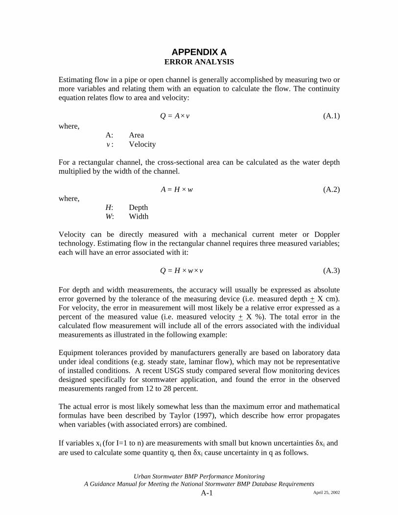
Estimating flow in a pipe or open channel is generally accomplished by measuring two or more variables and relating them with an equation to calculate the flow. The continuity equation relates flow to area and velocity:

vAQ ×= (A.1) where,

A: Area v : Velocity For a rectangular channel, the cross-sectional area can be calculated as the water depth multiplied by the width of the channel.

wHA ×= (A.2) where,

H: Depth W: Width

Velocity can be directly measured with a mechanical current meter or Doppler technology. Estimating flow in the rectangular channel requires three measured variables; each will have an error associated with it:

vwHQ ××= (A.3) For depth and width measurements, the accuracy will usually be expressed as absolute error governed by the tolerance of the measuring device (i.e. measured depth + X cm). For velocity, the error in measurement will most likely be a relative error expressed as a percent of the measured value (i.e. measured velocity + X %). The total error in the calculated flow measurement will include all of the errors associated with the individual measurements as illustrated in the following example: Equipment tolerances provided by manufacturers generally are based on laboratory data under ideal conditions (e.g. steady state, laminar flow), which may not be representative of installed conditions. A recent USGS study compared several flow monitoring devices designed specifically for stormwater application, and found the error in the observed measurements ranged from 12 to 28 percent. The actual error is most likely somewhat less than the maximum error and mathematical formulas have been described by Taylor (1997), which describe how error propagates when variables (with associated errors) are combined. If variables xi (for I=1 to n) are measurements with small but known uncertainties δxi and are used to calculate some quantity q, then δxi cause uncertainty in q as follows.

A-2


April 25, 2002

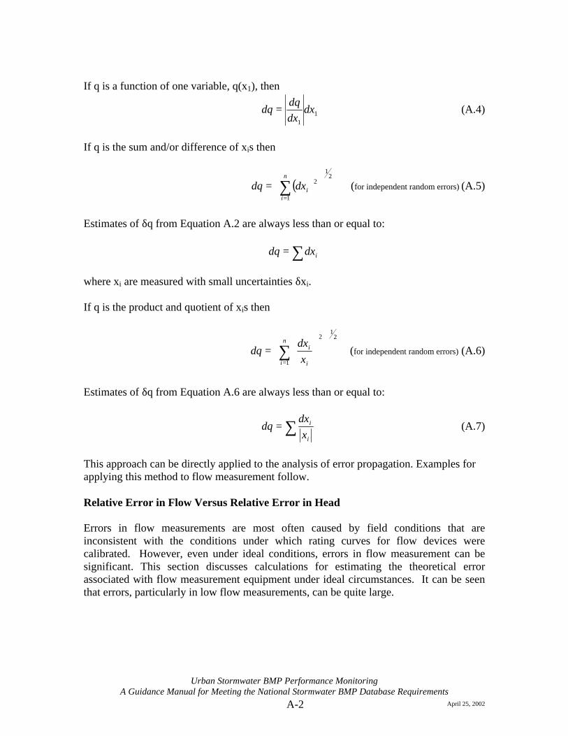
If q is a function of one variable, q(x1), then

11

xdxdq

q δδ = (A.4)

If q is the sum and/or difference of xis then

( )2

1

1

2

= ∑

=

n

iixq δδ (for independent random errors) (A.5)

Estimates of δq from Equation A.2 are always less than or equal to:

∑= ixq δδ

where xi are measured with small uncertainties δxi. If q is the product and quotient of xis then

21

1

2

= ∑

=

n

i i

i

xx

qδ

δ (for independent random errors) (A.6)

Estimates of δq from Equation A.6 are always less than or equal to:

∑=i

i

xx

qδ

δ (A.7)

This approach can be directly applied to the analysis of error propagation. Examples for applying this method to flow measurement follow. Relative Error in Flow Versus Relative Error in Head Errors in flow measurements are most often caused by field conditions that are inconsistent with the conditions under which rating curves for flow devices were calibrated. However, even under ideal conditions, errors in flow measurement can be significant. This section discusses calculations for estimating the theoretical error associated with flow measurement equipment under ideal circumstances. It can be seen that errors, particularly in low flow measurements, can be quite large.

A-3


April 25, 2002

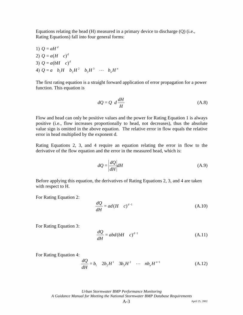
Equations relating the head (H) measured in a primary device to discharge (Q) (i.e., Rating Equations) fall into four general forms: 1) daHQ = 2) dcHaQ )( += 3) dcbHaQ )( += 4) n

n HbHbHbHbaQ +++++= L33

221

The first rating equation is a straight forward application of error propagation for a power function. This equation is

=

HH

dQQδ

δ (A.8)

Flow and head can only be positive values and the power for Rating Equation 1 is always positive (i.e., flow increases proportionally to head, not decreases), thus the absolute value sign is omitted in the above equation. The relative error in flow equals the relative error in head multiplied by the exponent d. Rating Equations 2, 3, and 4 require an equation relating the error in flow to the derivative of the flow equation and the error in the measured head, which is:

HdHdQ

Q δδ = (A.9)

Before applying this equation, the derivatives of Rating Equations 2, 3, and 4 are taken with respect to H. For Rating Equation 2:

1)( −+= dcHaddHdQ

(A.10)

For Rating Equation 3:

1)( −+= dcbHabddHdQ

(A.11)

For Rating Equation 4:

123

121 32 −++++= n

n HnbHbHbbdHdQ

L (A.12)

A-4


April 25, 2002

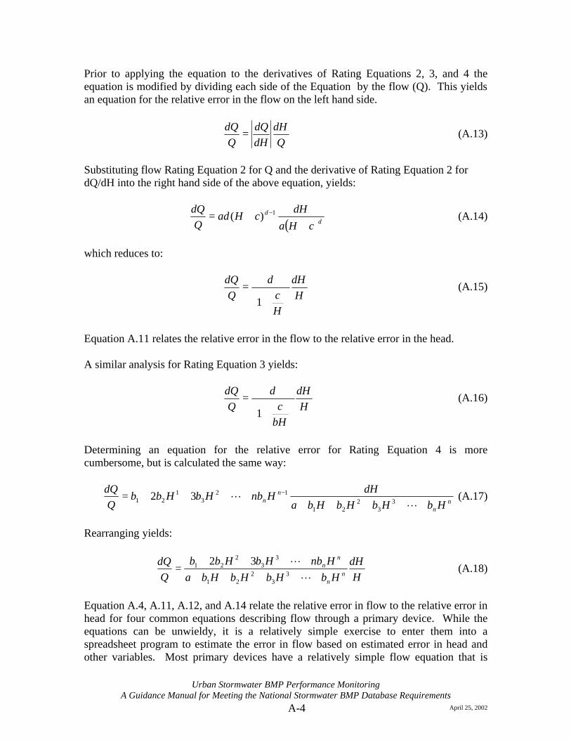
Prior to applying the equation to the derivatives of Rating Equations 2, 3, and 4 the equation is modified by dividing each side of the Equation by the flow (Q). This yields an equation for the relative error in the flow on the left hand side.

QH

dHdQ

QQ δδ

= (A.13)

Substituting flow Rating Equation 2 for Q and the derivative of Rating Equation 2 for dQ/dH into the right hand side of the above equation, yields:

( )dd

cHaH

cHadQQ

++= − δδ 1)( (A.14)

which reduces to:

HH

Hc

dQQ δδ

+

=1

(A.15)

Equation A.11 relates the relative error in the flow to the relative error in the head. A similar analysis for Rating Equation 3 yields:

HH

bHc

dQQ δδ

+

=1

(A.16)

Determining an equation for the relative error for Rating Equation 4 is more cumbersome, but is calculated the same way:

nn

nn HbHbHbHba

HHnbHbHbb

QQ

+++++++++= −

LL 3

32

21

123

121 32

δδ (A.17)

Rearranging yields:

HH

HbHbHbHbaHnbHbHbb

QQ

nn

nn δδ

+++++++++

=L

L3

32

21

33

221 32

(A.18)

Equation A.4, A.11, A.12, and A.14 relate the relative error in flow to the relative error in head for four common equations describing flow through a primary device. While the equations can be unwieldy, it is a relatively simple exercise to enter them into a spreadsheet program to estimate the error in flow based on estimated error in head and other variables. Most primary devices have a relatively simple flow equation that is

A-5


April 25, 2002

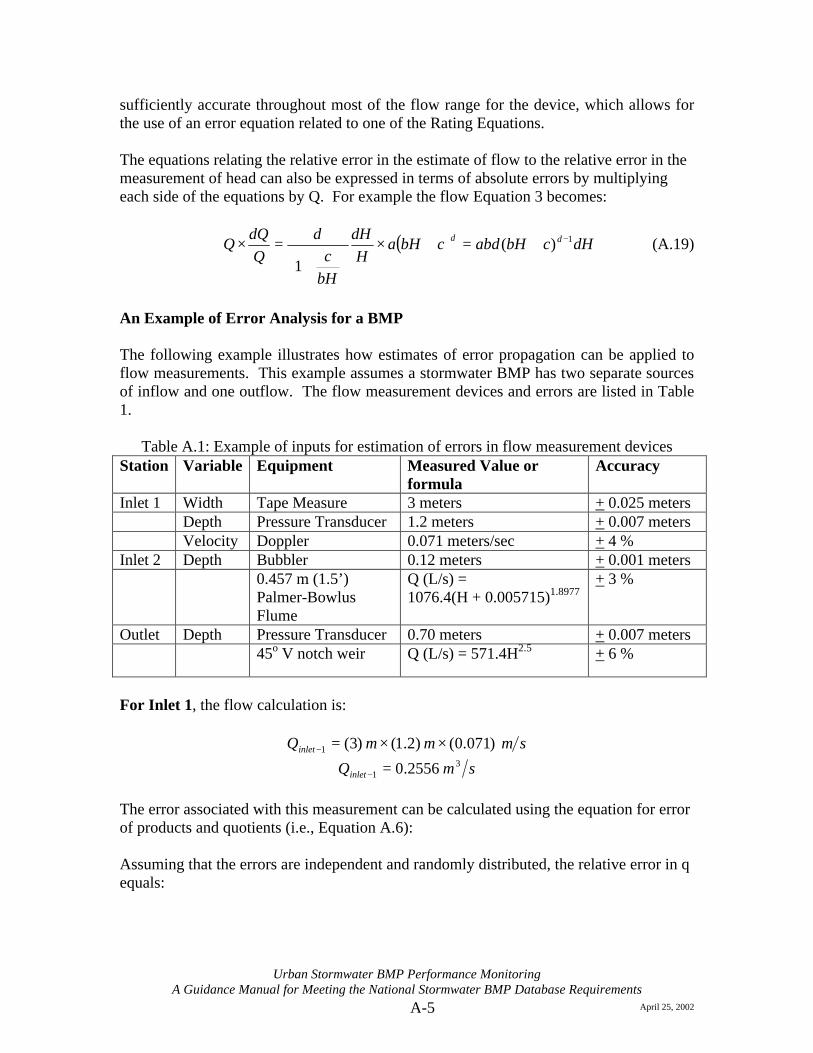
sufficiently accurate throughout most of the flow range for the device, which allows for the use of an error equation related to one of the Rating Equations. The equations relating the relative error in the estimate of flow to the relative error in the measurement of head can also be expressed in terms of absolute errors by multiplying each side of the equations by Q. For example the flow Equation 3 becomes:

( ) HcbHabdcbHaHH

bHc

dQQ

Q dd δδδ 1)(

1

−+=+×

+

=× (A.19)

An Example of Error Analysis for a BMP The following example illustrates how estimates of error propagation can be applied to flow measurements. This example assumes a stormwater BMP has two separate sources of inflow and one outflow. The flow measurement devices and errors are listed in Table 1.

Table A.1: Example of inputs for estimation of errors in flow measurement devices Station Variable Equipment Measured Value or

formula Accuracy

Inlet 1 Width Tape Measure 3 meters + 0.025 meters Depth Pressure Transducer 1.2 meters + 0.007 meters Velocity Doppler 0.071 meters/sec + 4 % Inlet 2 Depth Bubbler 0.12 meters + 0.001 meters 0.457 m (1.5’)

Palmer-Bowlus Flume

Q (L/s) = 1076.4(H + 0.005715)1.8977

+ 3 %

Outlet Depth Pressure Transducer 0.70 meters + 0.007 meters 45o V notch weir Q (L/s) = 571.4H2.5 + 6 %

For Inlet 1, the flow calculation is:

smmmQinlet )071.0( )2.1( )3(1 ××=−

smQinlet3

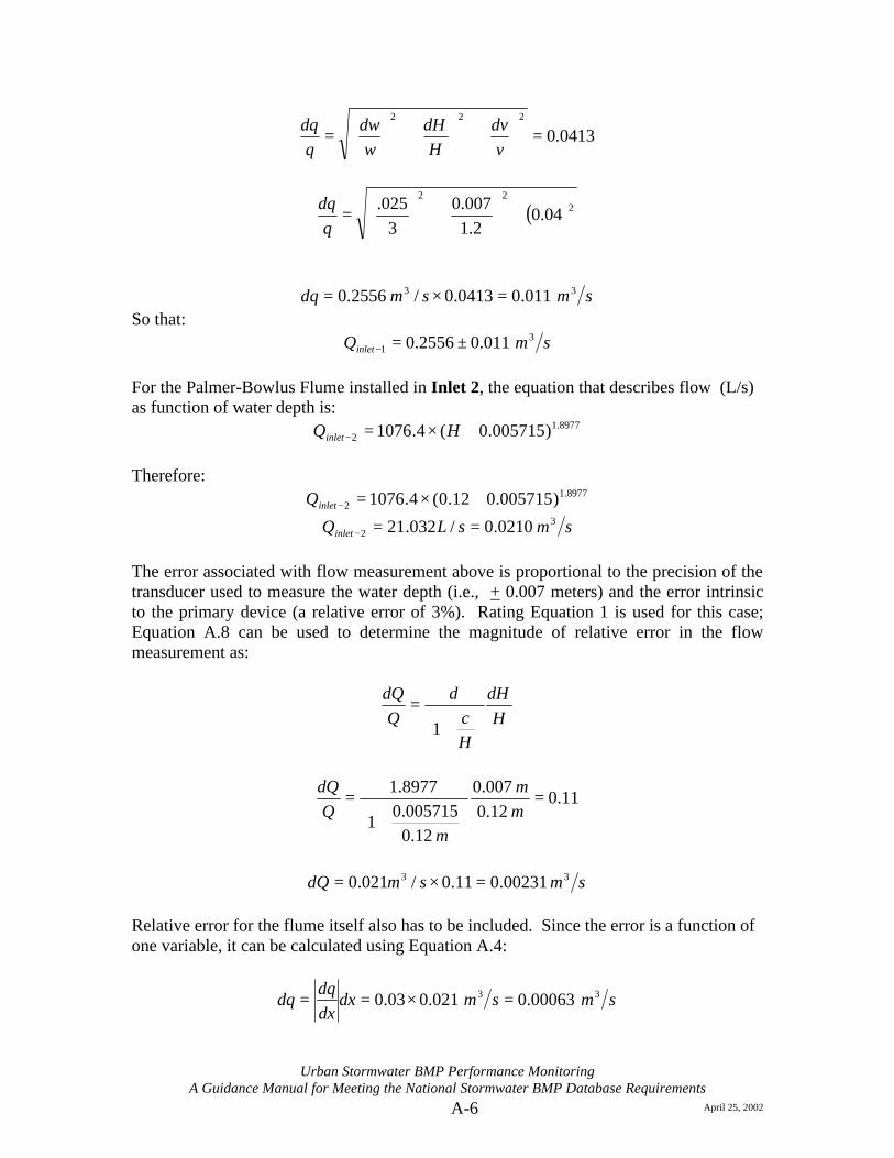
1 2556.0=− The error associated with this measurement can be calculated using the equation for error of products and quotients (i.e., Equation A.6): Assuming that the errors are independent and randomly distributed, the relative error in q equals:

A-6


April 25, 2002

0413.0222

=

+

+

=

vv

HH

ww

qq δδδδ

( )222

04.02.1

007.03

025.+

+

=

qqδ

smsmq 33 011.00413.0/ 2556.0 =×=δ So that:

smQinlet3

1 011.02556.0 ±=− For the Palmer-Bowlus Flume installed in Inlet 2, the equation that describes flow (L/s) as function of water depth is:

8977.12 )005715.0(4.1076 +×=− HQinlet

Therefore:

8977.12 )005715.012.0(4.1076 +×=−inletQ

smsLQinlet3

2 0210.0/032.21 ==− The error associated with flow measurement above is proportional to the precision of the transducer used to measure the water depth (i.e., + 0.007 meters) and the error intrinsic to the primary device (a relative error of 3%). Rating Equation 1 is used for this case; Equation A.8 can be used to determine the magnitude of relative error in the flow measurement as:

HH

Hc

dQQ δδ

+

=1

11.0 12.0 007.0

12.0005715.0

1

8977.1=

+

=mm

mQQδ

smsmQ 33 00231.011.0/021.0 =×=δ

Relative error for the flume itself also has to be included. Since the error is a function of one variable, it can be calculated using Equation A.4:

smsmxdxdq

q 33 00063.0 021.003.0 =×== δδ

A-7


April 25, 2002

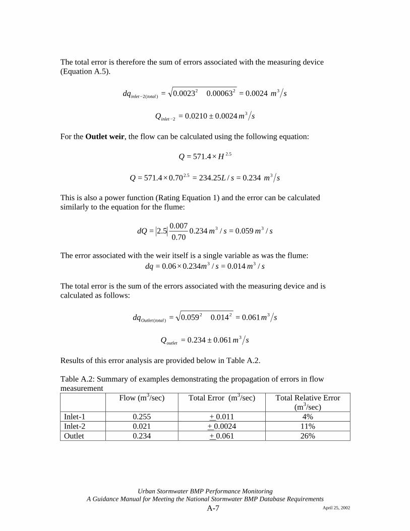
The total error is therefore the sum of errors associated with the measuring device (Equation A.5).

smq totalinlet322

)(2 0024.000063.00023.0 =+=−δ

smQinlet3

2 0024.00210.0 ±=− For the Outlet weir, the flow can be calculated using the following equation:

5.24.571 HQ ×=

smsLQ 35.2 234.0/25.23470.04.571 ==×= This is also a power function (Rating Equation 1) and the error can be calculated similarly to the equation for the flume:

smsmQ / 059.0/ 234.070.0

007.05.2 33 ==δ

The error associated with the weir itself is a single variable as was the flume:

smsmq / 014.0/234.006.0 33 =×=δ The total error is the sum of the errors associated with the measuring device and is calculated as follows:

smq totalOutlet322

)( 061.0014.0059.0 =+=δ

smQoutlet3 061.0234.0 ±=

Results of this error analysis are provided below in Table A.2. Table A.2: Summary of examples demonstrating the propagation of errors in flow measurement

Flow (m3/sec) Total Error (m3/sec) Total Relative Error (m3/sec)

Inlet-1 0.255 + 0.011 4% Inlet-2 0.021 + 0.0024 11% Outlet 0.234 + 0.061 26%

B-1

Urban Stormwater BMP Performance Monitoring

A Guidance Manual for Meeting the National Stormwater BMP Database Requirements April 25, 2002

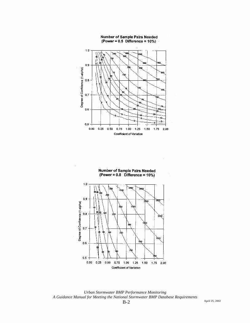
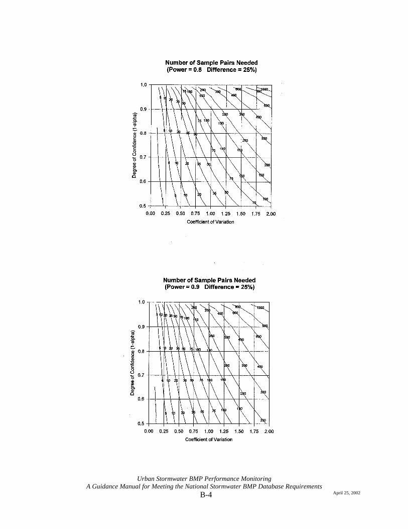
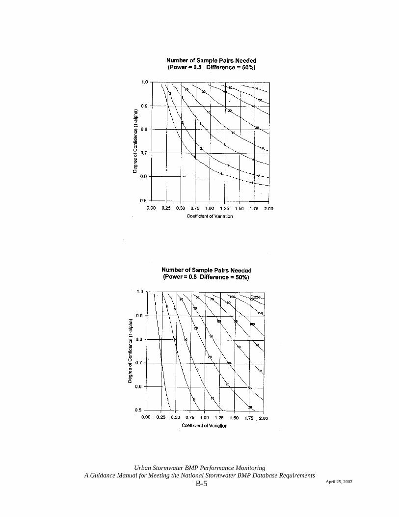
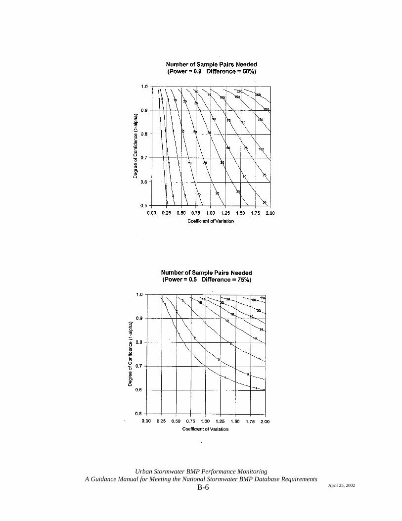
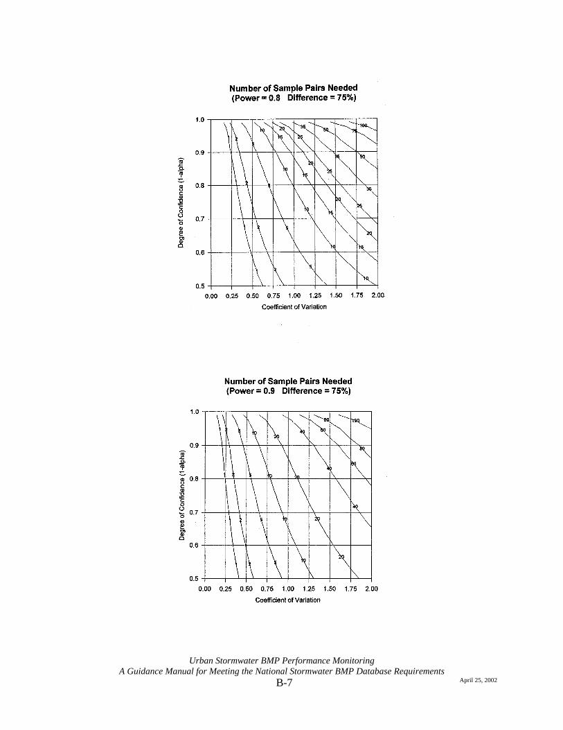
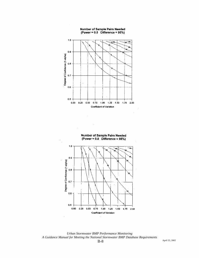
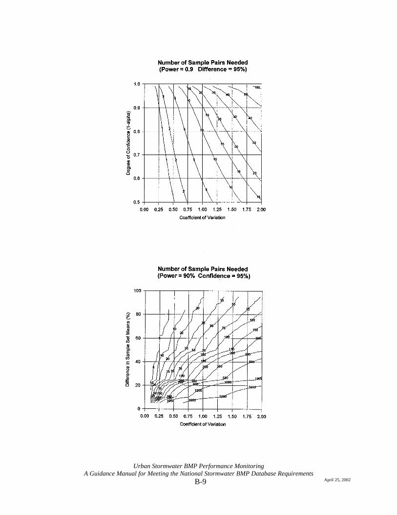
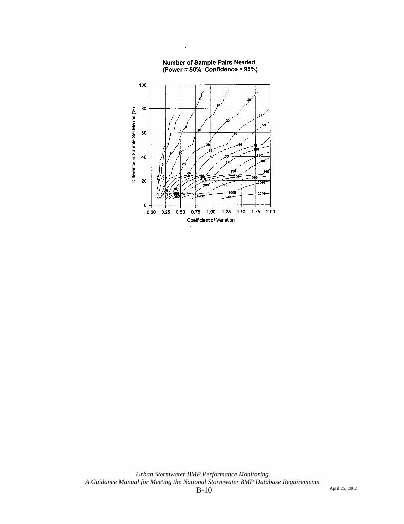
APPENDIX B NUMBER OF SAMPLES REQUIRED FOR VARIOUS POWERS, CONFIDENCE

INTERVALS, AND PERCENT DIFFERENCES The figures in this Appendix are from: R. Pitt and K. Parmer. Quality Assurance Project Plan (QAPP) for EPA Sponsored Study on Control of Stormwater Toxicants. Department of Civil and Environmental Engineering, University of Alabama at Birmingham. 1995.

B-2



B-3



B-4



B-5



B-6



B-7



B-8



B-9



B-10



C-1

Urban Stormwater BMP Performance Monitoring A Guidance Manual for Meeting the National Stormwater BMP Database Requirements April 25, 2002

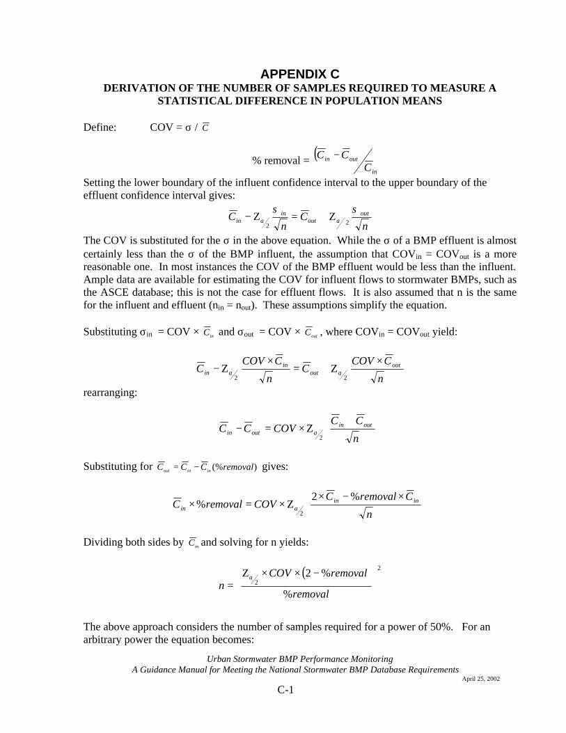
APPENDIX C DERIVATION OF THE NUMBER OF SAMPLES REQUIRED TO MEASURE A

STATISTICAL DIFFERENCE IN POPULATION MEANS

Define: COV = σ / C

% removal = ( )in

outin

CCC −

Setting the lower boundary of the influent confidence interval to the upper boundary of the effluent confidence interval gives:

nC

nC out

outin

in

σσαα 22

Ζ+=Ζ−

The COV is substituted for the σ in the above equation. While the σ of a BMP effluent is almost certainly less than the σ of the BMP influent, the assumption that COVin = COVout is a more reasonable one. In most instances the COV of the BMP effluent would be less than the influent. Ample data are available for estimating the COV for influent flows to stormwater BMPs, such as the ASCE database; this is not the case for effluent flows. It is also assumed that n is the same for the influent and effluent (nin = nout). These assumptions simplify the equation. Substituting σin = COV × inC and σout = COV × outC , where COVin = COVout yield:

n

CCOVC

n

CCOVC out

outin

in

×Ζ+=

×Ζ−

22αα

rearranging:

+Ζ×=−

n

CCCOVCC outin

outin2

α

Substituting for )(%removalCCC ininout −= gives:

×−×Ζ×=×

n

CremovalCCOVremovalC inin

in

%2%

2α

Dividing both sides by inC and solving for n yields:

( ) 2

2

%

%2

−××Ζ=

removal

removalCOVn

α

The above approach considers the number of samples required for a power of 50%. For an arbitrary power the equation becomes:

C-2

Urban Stormwater BMP Performance Monitoring A Guidance Manual for Meeting the National Stormwater BMP Database Requirements April 25, 2002

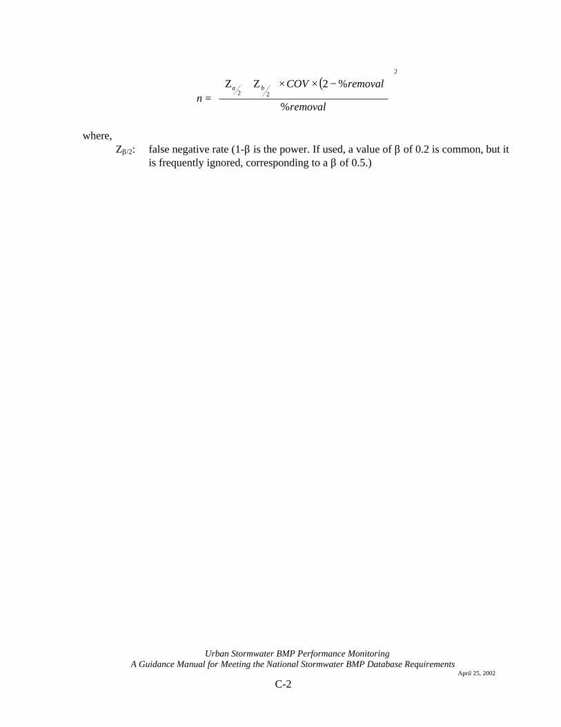
( )2

22

%

%2

−××

Ζ+Ζ

=removal

removalCOVn

βα

where, Zβ/2: false negative rate (1-β is the power. If used, a value of β of 0.2 is common, but it

is frequently ignored, corresponding to a β of 0.5.)

D-1


April 25, 2002

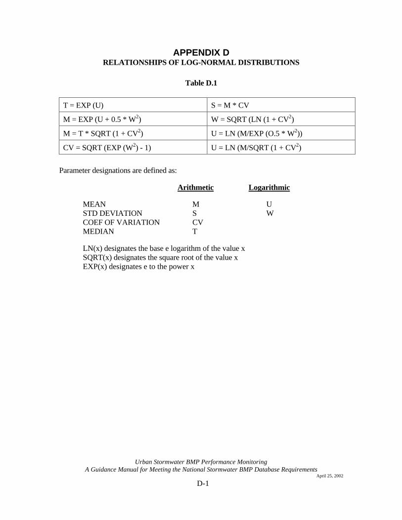
APPENDIX D RELATIONSHIPS OF LOG-NORMAL DISTRIBUTIONS

Table D.1

T = EXP (U) S = M * CV

M = EXP (U + 0.5 * W2) W = SQRT (LN (1 + CV2)

M = T * SQRT (1 + CV2) U = LN (M/EXP (O.5 * W2))

CV = SQRT (EXP (W2) - 1) U = LN (M/SQRT (1 + CV2)

Parameter designations are defined as:

Arithmetic Logarithmic

MEAN M U STD DEVIATION S W COEF OF VARIATION CV MEDIAN T

LN(x) designates the base e logarithm of the value x SQRT(x) designates the square root of the value x EXP(x) designates e to the power x

Documents

Urban Stormwater BMP Performance Monitoring - … · Urban Stormwater BMP Performance Monitoring ... National Stormwater Best Management Practices Database, ... Engineering Hydrology