Embed Size (px)
Citation preview
Optimization of BMP Selection for Distributed Stormwater
Treatment Networks
Clayton Christopher Hodges
Dissertation submitted to the faculty of the Virginia Polytechnic Institute and State
University in partial fulfillment of the requirements for the degree of
Doctor of Philosophy
In
Civil Engineering
Randel L. Dymond, Chair
Kathleen L. Hancock
Thomas J. Grizzard
David J. Sample
June 21, 2016
Blacksburg, Virginia
Keywords: Stormwater, best management practices (BMPs), selection optimization
Copyright © Clayton Christopher Hodges
Optimization of BMP Selection for Distributed Stormwater Treatment Networks
Clayton Christopher Hodges
ABSTRACT
Current site scale stormwater management designs typically include multiple
distributed stormwater best management practices (BMPs), necessary to meet regulatory
objectives for nutrient removal and groundwater recharge. Selection of the appropriate
BMPs for a particular site requires consideration of contributing drainage area
characteristics, such as soil type, area, and land cover. Other physical constraints such as
karst topography, areas of highly concentrated pollutant runoff, etc. as well as economics,
such as installation and operation and maintenance cost must be considered. Due to these
multiple competing selection criteria and regulatory requirements, selection of optimal
configurations of BMPs by manual iteration using conventional design tools is not
tenable, and the resulting sub-optimal solutions are often biased. This dissertation
addresses the need for an objective BMP selection optimization tool through definition of
an objective function, selection of an optimization algorithm based on defined selection
criteria, development of cost functions related to installation cost and operation and
maintenance cost, and ultimately creation and evaluation of a new software tool that
enables multi-objective user weighted selection of optimal BMP configurations.
A software tool is developed using the nutrient and pollutant removal logic found
in the Virginia Runoff Reduction Method (VRRM) spreadsheets. The resulting tool is
tested by a group of stormwater professionals from the Commonwealth of Virginia for
two case studies. Responses from case study participants indicate that use of the tool has
a significant impact on the current engineering design process for selection of stormwater
BMPs. They further indicate that resulting selection of stormwater BMPs through use of
the optimization tool is more objective than conventional methods of design, and allows
designers to spend more time evaluating solutions, rather than attempting to meet
regulatory objectives.

iii
DEDICATION
To my wife, Kacie, my sons, Elijah and Joel, and my parents, Allen and Peggy.
iv
ACKNOWLEDGEMENTS
The author would like to express gratitude to his advisor, Dr. Randel (Randy)
Dymond, for the opportunity to pursue a long time goal, and for his invaluable input on
this and other research. Adjusting back to an academic lifestyle after nearly two decades
working in industry was daunting, but Dr. Dymond’s guidance made it so much easier.
Dr. Dymond’s background in the software industry has proven invaluable over the course
of this dissertation in discussions concerning user interface, algorithmic selection, and
even nuances regarding the psychology of the learning process.
The author would also like to thank Dr. Hancock for her introduction and tutelage
in Geographic Information Systems (GIS). The skills that I have acquired from her
courses have given me new insight on manipulation of geographic data for scientific
study. Dr. Hancock also has a great ability to evaluate papers and determine issues with
context and gaps in coverage, even for articles that are somewhat out of her field of
expertise. Comments that I have received from Dr. Hancock on several papers have
aided me in modifying and improving my technical writing style.
Thanks is also given to Dr. Grizzard and Dr. Sample for serving on my
committee. I’ve had the opportunity to go to presentations with each several times over
the last couple of years. There have been many conversations regarding the current state
of the science behind stormwater BMP treatment technology. Both have a passion for
improving water quality for future generations.
The author would like to thank Kevin D. Young for his support through this
process. His guidance in review of articles, discussions regarding the theoretical aspects
of the topic, and friendship through this process has been invaluable.
The author especially wants to thank his wife and sons for making adjustments in
their lives and schedules to allow time for this pursuit. I want to thank my wife, sons,
and parents for their love and support through this process. I have missed soccer games,
track and cross country events, and weekend visits, and hope that I can repay their
patience with my own love and support in the future.
v
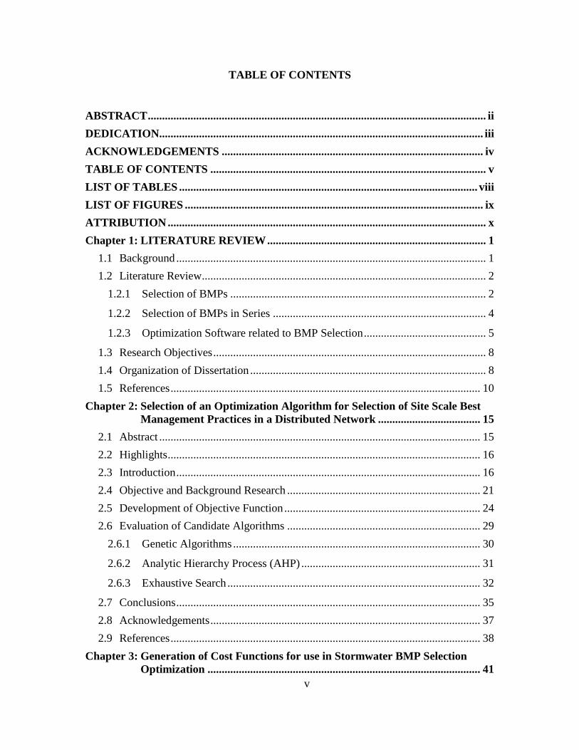
TABLE OF CONTENTS
ABSTRACT ....................................................................................................................... ii
DEDICATION.................................................................................................................. iii
ACKNOWLEDGEMENTS ............................................................................................ iv
TABLE OF CONTENTS ................................................................................................. v
LIST OF TABLES ......................................................................................................... viii
LIST OF FIGURES ......................................................................................................... ix
ATTRIBUTION ................................................................................................................ x
Chapter 1: LITERATURE REVIEW ............................................................................. 1
1.1 Background ............................................................................................................. 1
1.2 Literature Review.................................................................................................... 2
1.2.1 Selection of BMPs .......................................................................................... 2
1.2.2 Selection of BMPs in Series ........................................................................... 4
1.2.3 Optimization Software related to BMP Selection ........................................... 5
1.3 Research Objectives ................................................................................................ 8
1.4 Organization of Dissertation ................................................................................... 8
1.5 References ............................................................................................................. 10
Chapter 2: Selection of an Optimization Algorithm for Selection of Site Scale Best
Management Practices in a Distributed Network .................................... 15
2.1 Abstract ................................................................................................................. 15
2.2 Highlights .............................................................................................................. 16
2.3 Introduction ........................................................................................................... 16
2.4 Objective and Background Research .................................................................... 21
2.5 Development of Objective Function ..................................................................... 24
2.6 Evaluation of Candidate Algorithms .................................................................... 29
2.6.1 Genetic Algorithms ....................................................................................... 30
2.6.2 Analytic Hierarchy Process (AHP) ............................................................... 31
2.6.3 Exhaustive Search ......................................................................................... 32
2.7 Conclusions ........................................................................................................... 35
2.8 Acknowledgements ............................................................................................... 37
2.9 References ............................................................................................................. 38
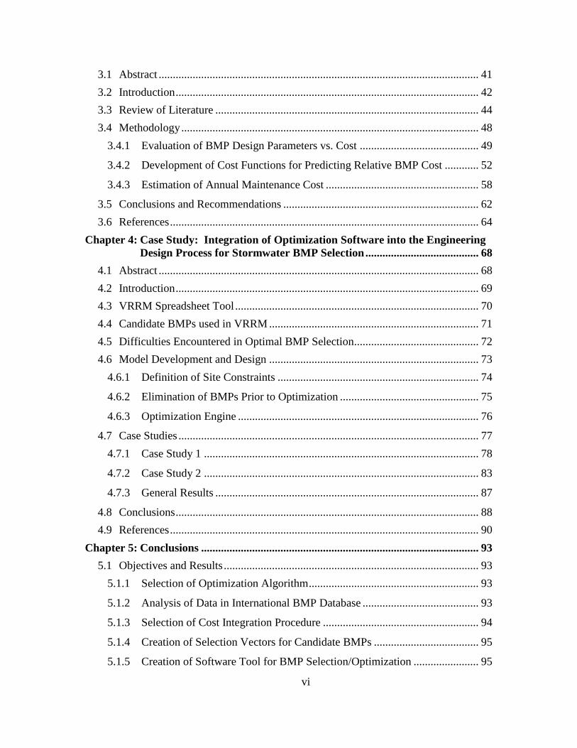
Chapter 3: Generation of Cost Functions for use in Stormwater BMP Selection
Optimization ................................................................................................ 41
vi
3.1 Abstract ................................................................................................................. 41
3.2 Introduction ........................................................................................................... 42
3.3 Review of Literature ............................................................................................. 44
3.4 Methodology ......................................................................................................... 48
3.4.1 Evaluation of BMP Design Parameters vs. Cost .......................................... 49
3.4.2 Development of Cost Functions for Predicting Relative BMP Cost ............ 52
3.4.3 Estimation of Annual Maintenance Cost ...................................................... 58
3.5 Conclusions and Recommendations ..................................................................... 62
3.6 References ............................................................................................................. 64
Chapter 4: Case Study: Integration of Optimization Software into the Engineering
Design Process for Stormwater BMP Selection ........................................ 68
4.1 Abstract ................................................................................................................. 68
4.2 Introduction ........................................................................................................... 69
4.3 VRRM Spreadsheet Tool ...................................................................................... 70
4.4 Candidate BMPs used in VRRM .......................................................................... 71
4.5 Difficulties Encountered in Optimal BMP Selection............................................ 72
4.6 Model Development and Design .......................................................................... 73
4.6.1 Definition of Site Constraints ....................................................................... 74
4.6.2 Elimination of BMPs Prior to Optimization ................................................. 75
4.6.3 Optimization Engine ..................................................................................... 76
4.7 Case Studies .......................................................................................................... 77
4.7.1 Case Study 1 ................................................................................................. 78
4.7.2 Case Study 2 ................................................................................................. 83
4.7.3 General Results ............................................................................................. 87
4.8 Conclusions ........................................................................................................... 88
4.9 References ............................................................................................................. 90
Chapter 5: Conclusions .................................................................................................. 93
5.1 Objectives and Results .......................................................................................... 93
5.1.1 Selection of Optimization Algorithm ............................................................ 93
5.1.2 Analysis of Data in International BMP Database ......................................... 93
5.1.3 Selection of Cost Integration Procedure ....................................................... 94
5.1.4 Creation of Selection Vectors for Candidate BMPs ..................................... 95
5.1.5 Creation of Software Tool for BMP Selection/Optimization ....................... 95
vii
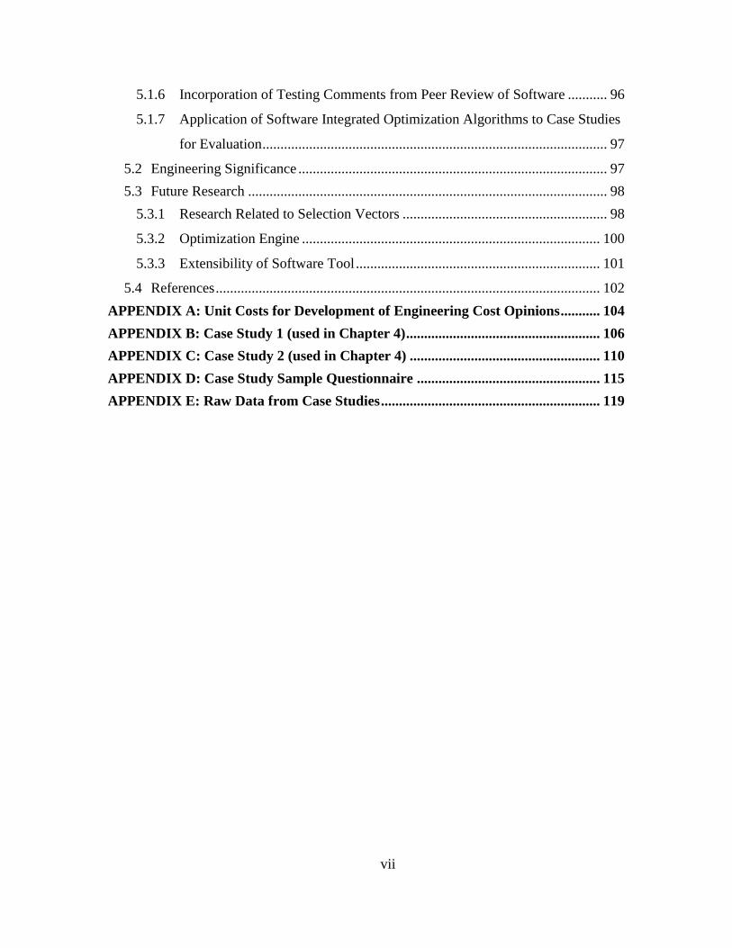
5.1.6 Incorporation of Testing Comments from Peer Review of Software ........... 96
5.1.7 Application of Software Integrated Optimization Algorithms to Case Studies
for Evaluation ................................................................................................ 97
5.2 Engineering Significance ...................................................................................... 97
5.3 Future Research .................................................................................................... 98
5.3.1 Research Related to Selection Vectors ......................................................... 98
5.3.2 Optimization Engine ................................................................................... 100
5.3.3 Extensibility of Software Tool .................................................................... 101
5.4 References ........................................................................................................... 102
APPENDIX A: Unit Costs for Development of Engineering Cost Opinions ........... 104
APPENDIX B: Case Study 1 (used in Chapter 4) ...................................................... 106
APPENDIX C: Case Study 2 (used in Chapter 4) ..................................................... 110
APPENDIX D: Case Study Sample Questionnaire ................................................... 115
APPENDIX E: Raw Data from Case Studies ............................................................. 119
viii
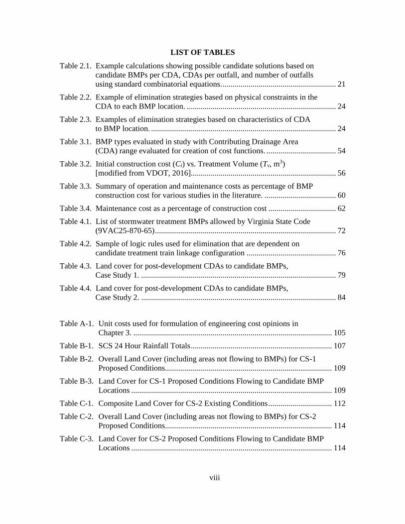
LIST OF TABLES
Table 2.1. Example calculations showing possible candidate solutions based on
candidate BMPs per CDA, CDAs per outfall, and number of outfalls
using standard combinatorial equations. ......................................................... 21
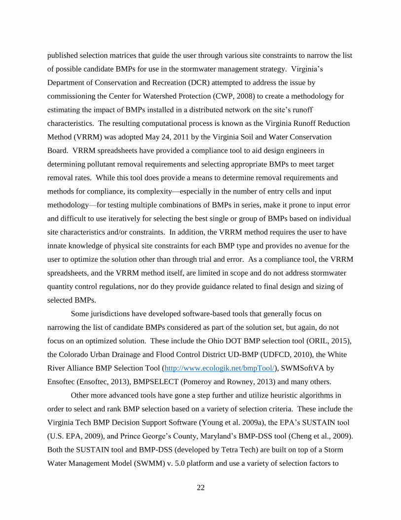
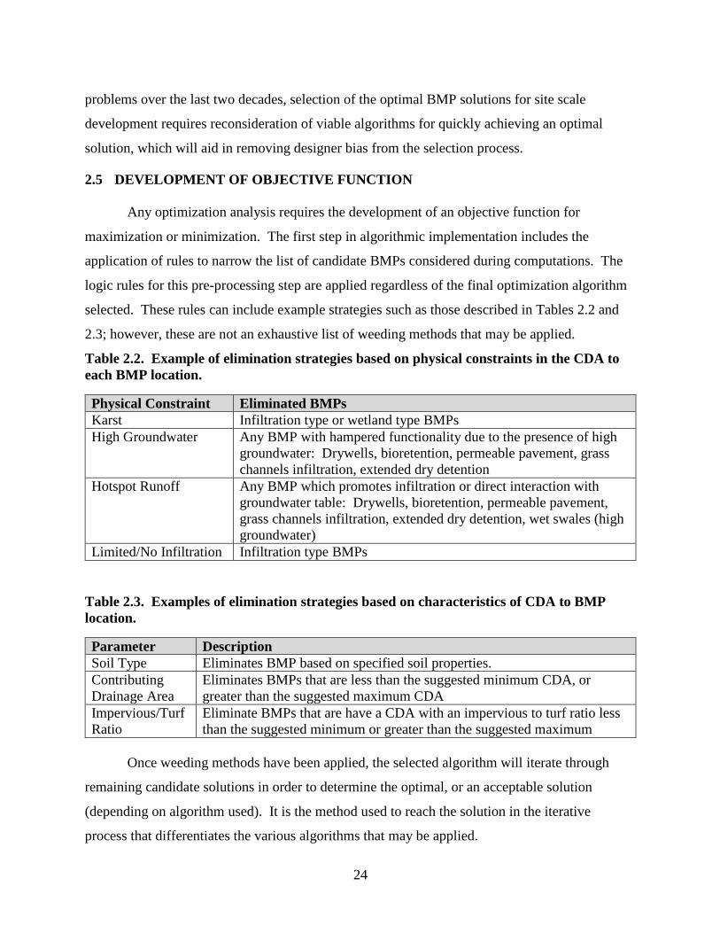
Table 2.2. Example of elimination strategies based on physical constraints in the
CDA to each BMP location. ........................................................................... 24
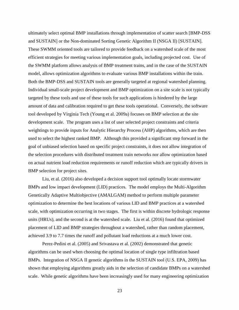
Table 2.3. Examples of elimination strategies based on characteristics of CDA
to BMP location. ............................................................................................. 24
Table 3.1. BMP types evaluated in study with Contributing Drainage Area
(CDA) range evaluated for creation of cost functions. ................................... 54
Table 3.2. Initial construction cost (Ci) vs. Treatment Volume (Tv, m3)
[modified from VDOT, 2016]......................................................................... 56
Table 3.3. Summary of operation and maintenance costs as percentage of BMP
construction cost for various studies in the literature. .................................... 60
Table 3.4. Maintenance cost as a percentage of construction cost .................................. 62
Table 4.1. List of stormwater treatment BMPs allowed by Virginia State Code
(9VAC25-870-65) ........................................................................................... 72
Table 4.2. Sample of logic rules used for elimination that are dependent on
candidate treatment train linkage configuration ............................................. 76
Table 4.3. Land cover for post-development CDAs to candidate BMPs,
Case Study 1. .................................................................................................. 79
Table 4.4. Land cover for post-development CDAs to candidate BMPs,
Case Study 2. .................................................................................................. 84
Table A-1. Unit costs used for formulation of engineering cost opinions in
Chapter 3. .................................................................................................... 105
Table B-1. SCS 24 Hour Rainfall Totals ....................................................................... 107
Table B-2. Overall Land Cover (including areas not flowing to BMPs) for CS-1
Proposed Conditions .................................................................................... 109
Table B-3. Land Cover for CS-1 Proposed Conditions Flowing to Candidate BMP
Locations ..................................................................................................... 109
Table C-1. Composite Land Cover for CS-2 Existing Conditions ................................ 112
Table C-2. Overall Land Cover (including areas not flowing to BMPs) for CS-2
Proposed Conditions .................................................................................... 114
Table C-3. Land Cover for CS-2 Proposed Conditions Flowing to Candidate BMP
Locations ..................................................................................................... 114
ix
LIST OF FIGURES
Figure 2.1. Schematic layout of treatment train demonstrating component input. .......... 18
Figure 2.2. Categorized classifications of non-proprietary stormwater BMPs ................ 20
Figure 2.3. Frequency and cumulative distribution of active projects (March 2016)
in the Commonwealth of Virginia from permit holder composite list,
data from (VDEQ, 2016). .............................................................................. 34
Figure 2.4. Semi-log plot depicting computational time to iterate through candidate
solutions for two test processors. .................................................................. 35
Figure 3.1. Construction cost vs. treatment volume. Resulting cost functions are in
grayscale behind hatched cost regions for each BMP group. ........................ 55
Figure 3.2. Linear functions fit through cost estimate points for Level 1 and 2
bioretention .................................................................................................... 57
Figure 3.3. Sensitivity of Bioretention Level 1 to fluctuations in estimated soil media
unit cost (85% - 115% of average unit cost used in estimates). .................... 58
Figure 4.1. Example of node and link input model integrated as part of BMP layout
functionality of tool. ...................................................................................... 74
Figure 4.2. Post-development CDAs to candidate BMP locations for Case Study 1. ..... 79
Figure 4.3. Frequency histograms indicating (a) usability (b) constraint
consideration, and (c) perception of improved design capabilities
for CS1. ......................................................................................................... 82
Figure 4.4. Post-development CDAs to candidate BMP locations for Case Study 2.
Arrows indicate direction of flow if BMPs are linked in a treatment train
configuration. ................................................................................................ 84
Figure 4.5. Frequency histograms indicating (a) usability (b) constraint
consideration, and (c) perception of improved design capabilities
for CS2. ......................................................................................................... 86
Figure B-1. CS-1 – Existing Conditions ....................................................................... 107
Figure B-2. CS-1 – Concept Layout with Potential BMP Locations ............................ 108
Figure C-1. CS-2 – Existing Conditions (Prior to Phase I Construction) ..................... 111
Figure C-2. CS-2 – Proposed Development Conditions with Preliminary
Locations of Stormwater BMPs ................................................................. 113
x
ATTRIBUTION
The contributions of authors of manuscripts included as major chapters in this
dissertation are listed below.
Clayton C. Hodges, P.E., PhD Candidate
The Charles E. Via, Jr. Department of Civil and Environmental Engineering
Virginia Polytechnic Institute and State University, Blacksburg, VA, 24061
Corresponding/Lead author of Chapters 2 – 4. Participated in development of research
design (objectives and hypothesis). Participated in the development of objective function
for algorithm integration, development of cost functions, coded the selection optimization
tool. Created all relevant figures, exhibits, and tables for inclusion in manuscripts for
submission to journals. Prepared research protocol (emails, case study problems,
questionnaires).
Randel L. Dymond, PhD, P.E., Associate Professor
The Charles E. Via, Jr. Department of Civil and Environmental Engineering
Virginia Polytechnic Institute and State University, Blacksburg, VA, 24061
Coauthor of Chapters 2 – 4. Participated in development of research design (objectives
and hypothesis). Reviewed procedures, data, selection methods. Assisted in software
testing. Provided review for all materials related to research protocol. Reviewed,
provided revisions, and contributions to journal manuscripts.
Kevin D. Young, P.E., Professor of Practice
The Charles E. Via, Jr. Department of Civil and Environmental Engineering
Virginia Polytechnic Institute and State University, Blacksburg, VA, 24061
Coauthor of Chapters 3 and 4. Contributed significantly to development of cost functions
in Chapter 3. Assisted in software testing. Assisted in implementing research protocol in
Chapter 4. Reviewed, provided revisions, and contributions to journal manuscripts.
1
Chapter 1: LITERATURE REVIEW
1.1 BACKGROUND
After enactment of the Clean Water Act (33 U.S.C §1251 et seq., 1972), the creation of
the National Pollutant Discharge Elimination System (NPDES) as administered by the United
States Environmental Protection Agency (USEPA) began a paradigm shift in stormwater
management as it relates to urban development projects. Conventional methods of stormwater
management, at the time, dealt primarily with peak flow and erosion control. Large surface
storage facilities that shaved peak flows and promoted gravitational settling of suspended solids
through extended detention of the treatment volume were the norm. Though the treatment
volume was detained, it was not reduced, which resulted in accelerated degradation of
downstream channels as development proceeded.
Amendments to the Clean Water Act (CWA) were enacted in 1977, 1981, and 1987 to
clarify the scope (Clarke, 2003) and applicability on a national level, with the Water Quality Act
of 1987 (CWA Section 319) becoming a cornerstone of today’s stormwater management
regulations. Roll-out of the regulations took place in two phases, with larger Phase I Municipal
Separate Storm Sewer Systems (MS4s) required to comply first, in the early 1990’s. Smaller
Phase II MS4s were required to comply with the new standards that placed limitations on
pollutant discharges in the early 2000’s. A new wave of stormwater best management practices
(BMPs) resulted from these new water quality discharge requirements, resulting in the
implementation of measures such as bioretention (rain gardens), sand filters, constructed
wetlands, and others, in an effort to reduce the impact of pollutant loads on the nation’s waters.
Later, research by Shuster et al. (2007), Li et al. (2009), Balascio and Lucas (2009), and
many others, focused on stormwater management through replication of a site’s predevelopment
hydrologic response. Burns et al. (2012) stated that focus should be placed on development of
sites using low impact development (LID) strategies. LID techniques integrated in development
focus on 1) minimization of disturbance, 2) limiting large connected impervious areas, and 3)
promoting runoff reduction through groundwater recharge or evapotranspiration, which
combined can have a huge impact on the quality of effluent from a developed site to a receiving
2
channel/stream. As described by Elliott and Trowsdale (2007), LID strategies have ushered in
the use of distributed small scale stormwater management BMPs throughout a developed site.
1.2 LITERATURE REVIEW
Below is an abbreviated literature review related to the major research components that
are part of this dissertation. More extensive background on each topic can be found in
comparable sections of Chapters 2-4.
1.2.1 Selection of BMPs
The USEPA first released a ‘National Menu of Best Management Practices (BMPs) for
Stormwater’ (USEPA, 2016) in October 2000, which forms the basis of BMP standards in most
states. The standards include non-structural BMPs such as minimization strategies, and
structural practices, such as permeable pavement, grassed swales, infiltration basins,
bioretention, etc. The resulting list of strategies provides many viable options to a stormwater
management designer for treating effluent prior to discharge from developed sites. Ellis et al.
(2004) note that there are many factors that must be considered during selection of BMPs,
including technical requirements, social benefits, costs, and environmental impacts.
Technical requirements in BMP selection includes choosing the appropriate BMP to meet
regulatory pollutant objectives. In some jurisdictions, a mandatory reduction in postdevelopment
runoff volume is also required. Physical constraints can include the properties of the
contributing drainage area (CDA), including size, land cover, slope, soil properties, (Young et
al., 2010), and subsurface properties such as karst, high groundwater, etc. Selection may also be
affected by a desire to add social incentives, such as the aesthetic benefits associated with some
BMPs. As with most components in urban development, the effect of cost during the BMP
selection process usually plays a major role in stormwater management. Due to the number of
available BMPs, competing selection strategies, and physical siting constraints, more efficient
strategies and tools are required to ensure that the most appropriate BMP(s) are selected after
weighing these criteria.
Initial attempts at guiding BMP selection can be found in government publications
including BMP specifications which defined individual BMP recommendations. Most states
include selection tables or matrices in their BMP design handbooks, including North Carolina
(NCDENR, 2007), Maryland (MDE, 2009), West Virginia (WVDEP, 2012), Virginia (VDEQ,
3
2013), and others. Later, there were attempts by university groups, government agencies, and
other third party sources to attempt to develop BMP selection tools to streamline the selection
and/or life cycle cost evaluation of specific BMP installations. Those addressing BMP selection
include the Ohio DOT BMP selection tool (ORIL, 2015), the Colorado Urban Drainage and
Flood Control District UD-BMP (UDFCD, 2010), the White River Alliance (WRA, 2016) BMP
Selection Tool, and several others. Most of these tools are simple web-based or spreadsheet
based tools that allow the user to indicate if various site features and/or constraints are present on
the project site. From this user input, many BMPs are eliminated from consideration, leaving the
user with a candidate list of BMPs that may be suitable for the project. Other tools also integrate
regulatory removal requirements into the selection strategy, and eliminate practices that cannot
meet the required removals. The net result from either strategy is the generation of a refined list
of candidate BMPs that are suitable for the site. At this point, it is the designer’s responsibility
to use their ‘best judgement’ in selecting the most appropriate BMPs for the site from this list.
Other efforts have focused not only on performance, but cost analysis related to BMP
selection. Some of these tools include BMP-REALCOST (UDFCD, 2010), the National
Cooperative Highway Research Program life cycle spreadsheets (Taylor et al. 2014), and the
WERF SELECT tool (Pomeroy and Rowney, 2013). BMP-REALCOST was developed as a
planning level tool that uses input to estimate how many single type BMP installations would be
necessary to treat a region, and from that prediction provide life cycle cost estimates for those
installations. The National Cooperative Highway Research Program [NCHRP] (Taylor et al.,
2014) attempts to address the issue of calculation of capital cost and life cycle cost associated
with retrofit of highway BMPs in its Report 792. The purpose of the report is to provide a
framework and tools for the user to perform cost analysis for particular BMP installations. The
database used for costs in the report is a consolidation of data from the International Stormwater
BMP Database (ISBMPD, 2014) and various other cost studies. The WERF SELECT model
(Pomeroy and Rowney, 2013) is also a regional planning tool that allows life cycle cost analysis
for a specified region. In addition to cost estimates, the WERF model also has built-in
functionality to estimate various water quality treatment parameters such as load reduction and
runoff reduction based on specified installations within the region.
The cost tools previously described use different methods to generate cost estimates for
BMP comparison. Capital (installation) costs are typically either estimated based on statistical
4
analysis of past installations, or through the integration of engineering cost opinions which take
into account more local unit costs for BMP components. WERF (2005) concluded that it is not
likely that computation of construction costs would benefit from a national cost database. This is
due to difficulties in standardizing reporting of costs, and the inability to take into account all of
the regional variations associated with costs. Despite this assertion, the International Stormwater
BMP Database (ISBMPD, 2014), does provide records regarding BMP performance and cost.
An analysis of ISBMPD (2014), however, yields only a small sample (145) of records that
indicate cost data of any kind, of which, only 49 records include initial construction cost, spread
over multiple BMP types. Lack of sample size and unknown consistency and variability related
to these entries make it difficult to rely on this data for accurate estimations of BMP installation
cost.
Initial construction cost may not be the most important cost factor in BMP selection,
since operating and maintenance (O&M) costs can also be significant. USEPA (1999) reported
O&M cost as a percentage of initial construction cost, based on a statistical analysis of the work
by Wiegand et al. (1986), Schueler (1987), SWRPC (1991), Livingston et al. (1997), and Brown
and Schueler (1997). Weiss et al. (2007) and King and Hagan (2011) support the estimation of
O&M costs as a percentage of initial construction costs. Others, such as Taylor et al. (2015) and
WERF (2005) attempt to estimate common maintenance activities and material and labor costs in
order to compute a net present values (NPV) cost associated with long term maintenance.
1.2.2 Selection of BMPs in Series
Increasing use of smaller distributed BMPs throughout development sites has resulted in
interconnection of these practices in many instances, which can allow for additional treatment in
downstream BMPs. Hathaway and Hunt (2010) discuss the use of wetland cells in series in
treating stormwater runoff. Villarreal et al. (2004) examine a series of stormwater treatment
cells at reducing runoff in an urban environment. Cascading treatment of stormwater runoff
requires a method of tracking pollutant and runoff reduction through each node. Pennsylvania
(PADEP, 2006), published equations for tracking effluent loads through BMPs installed in
parallel or in series. Hirschman et al. (2008) published a method known as the Runoff Reduction
Method (RRM), which was used in the development of the Virginia Runoff Reduction Method
spreadsheets (VDEQ, 2016), that enables the user to input and track pollutants and runoff
reduction through connected BMP configuration, also called ‘treatment trains’ (Wong et al.,
5
2006). Commercial software packages, such as SWMSoftVA (Ensoftec, 2013) have recently
been produced which integrate the runoff and pollutant tracking capability of the VRRM
Spreadsheets (VDEQ, 2016), with constraint input, which allows elimination of BMPs based on
physical constraints, while performing calculations to determine if regulatory thresholds have
been met.
Integration of treatment trains in computation methods for stormwater management has
allowed for additional effluent treatment prior to discharge from the site, but has also shed light
on several issues related to BMP treatment strategies. Work by Hathaway and Hunt (2010) was
performed to confirm that 1) treatment efficiencies are related to the event mean concentration
(EMC) of incoming runoff, and 2) secondary mechanical treatment becomes ineffective as the
EMC approaches an irreducible concentration value, which varies between pollutants. Published
methods of computation for most states ignore both of these items, opting instead to recommend
use of static removal efficiencies, and not address the irreducible concentration of pollutants.
The state of Delaware (DNREC, 2008) does address the issue of irreducible concentrations, and
has developed a simplified method of restricting additional mechanical treatment beyond this
level. DNREC (2008) lists the irreducible concentration of phosphorus as 0.11 mg/l, and that of
nitrogen as 1.2 mg/l, while work by Schueler and Holland (2000) indicates that irreducible
concentrations for total phosphorus are between 0.15 mg/L and 0.20 mg/L, for total nitrogen, 1.9
mg/L, and for total suspended solids, between 20 mg/L to 40 mg/L. Note that the irreducible
concentrations listed above are related to physical removal of further concentration from
stormwater runoff; however, additional removal beyond this irreducible concentration can be
achieved on a mass load basis through runoff reduction.
1.2.3 Optimization Software related to BMP Selection
Sections 1.2.1 and 1.2.2 discuss BMP selection tools that aid the user by decreasing the
number of viable BMP candidates through input of various constraints. Other more advanced
tools have gone a step further and integrate algorithms to automate the BMP selection process
based on a variety of criteria. These include the Virginia Tech BMP Decision Support Software
(Young et al. 2009), the SUSTAIN tool by EPA (U.S. EPA, 2011), Prince George’s County,
Maryland’s BMP-DSS tool (Cheng et al., 2009), and a multi-objective BMP siting tool by Liu et
al. (2016). Both the SUSTAIN tool and BMP-DSS are built on top of a Storm Water
Management Model (SWMM) v. 5.0 platform, are integrated into ESRI ArcMap 9.3, and use a
6
variety of selection factors to ultimately select optimal BMP installations through
implementation of scatter search [BMP-DSS and SUSTAIN] or the Non-Dominated Sorting
Genetic Algorithm II (NSGA II) [SUSTAIN]. BMP-DSS and SUSTAIN are tailored to be
regional watershed planning tools and are used to provide feedback on a watershed scale of the
most efficient strategies for meeting various implementation goals, including projected cost. Use
of the SWMM platform allows analysis of BMP treatment trains, and in the case of the
SUSTAIN model, allows optimization algorithms to evaluate various predefined BMP
configurations within the train. BMP-DSS, SUSTAIN, and the tool by Liu et al. are targeted at
regional watershed planning. Individual small-scale project development and BMP optimization
on a site scale is not targeted by these tools.
The decision support software tool developed by Virginia Tech (Young et al. 2009)
focuses on BMP selection at the site development scale. The program uses a list of user selected
project constraints and criteria weightings to provide inputs for Analytic Hierarchy Process
(AHP) algorithms, which are then used to select the highest ranked BMP. Although this decision
support software (DSS) provides a significant step forward in the goal of unbiased selection
based on specific project constraints, it does not allow integration of the selection procedures
with treatment train networks nor allow optimization based on actual load reduction or runoff
reduction requirements which are typically drivers in BMP selection for project sites.
1.2.3.1 Optimization Algorithms
Recently, there has been a surge of engineering optimization problems that have been
solved using genetic algorithms (GAs). These algorithms were first proposed by Holland (1975)
and operate using rules and techniques borrowed from the natural world. Many fall under a
category known as evolutionary algorithms in which the population is based on candidate
solutions, with each successive generation [hopefully] approaching the optimal solution based on
predefined fitness functions. This method uses principles such as genetic crossover, random
mutation of a portion of the population, and other techniques for ‘breeding’ new generations
closer to the optimal solution. There are also other genetic algorithms, such as firefly
optimization (Sayadi et al., 2010), ant colony optimization (Di Caro and Gambardella, 1999),
and others that have been successfully employed on past problems.
7
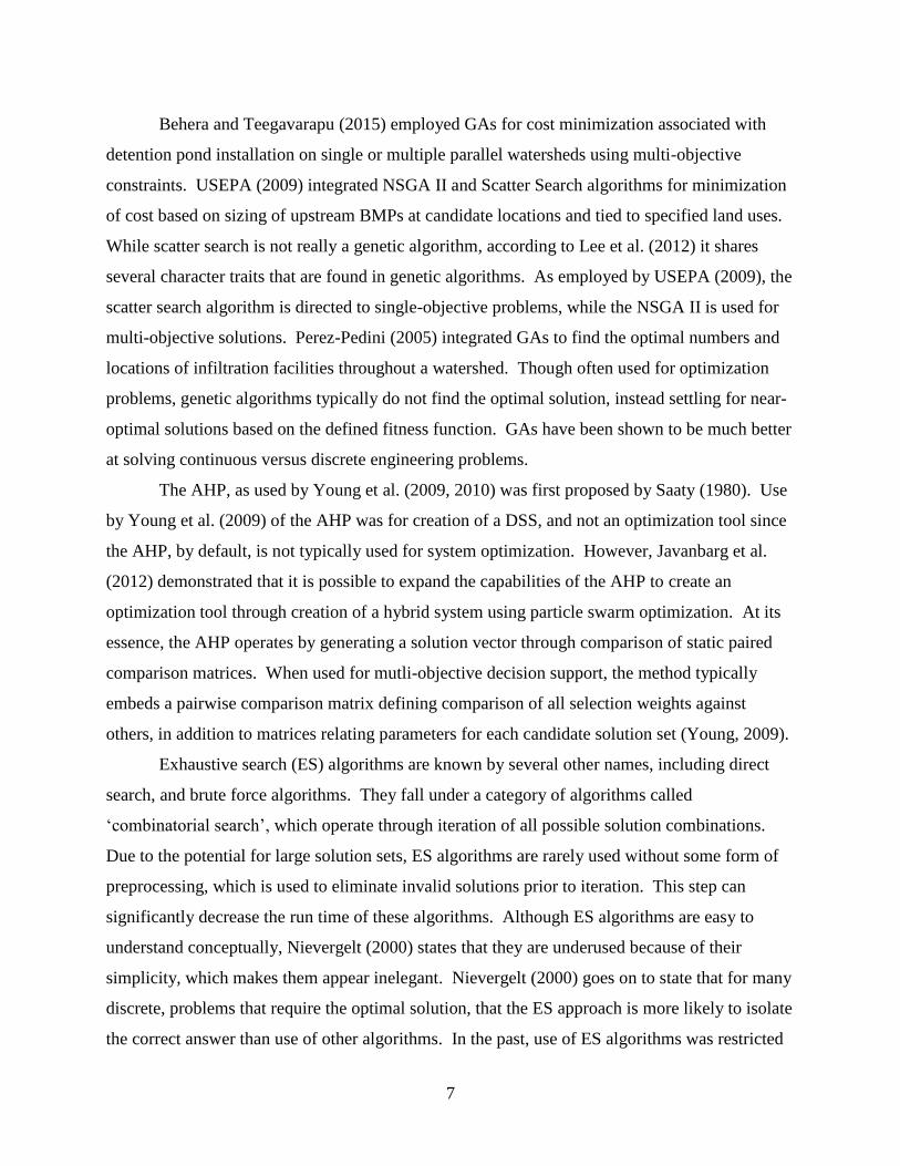
Behera and Teegavarapu (2015) employed GAs for cost minimization associated with
detention pond installation on single or multiple parallel watersheds using multi-objective
constraints. USEPA (2009) integrated NSGA II and Scatter Search algorithms for minimization
of cost based on sizing of upstream BMPs at candidate locations and tied to specified land uses.
While scatter search is not really a genetic algorithm, according to Lee et al. (2012) it shares
several character traits that are found in genetic algorithms. As employed by USEPA (2009), the
scatter search algorithm is directed to single-objective problems, while the NSGA II is used for
multi-objective solutions. Perez-Pedini (2005) integrated GAs to find the optimal numbers and
locations of infiltration facilities throughout a watershed. Though often used for optimization
problems, genetic algorithms typically do not find the optimal solution, instead settling for near-
optimal solutions based on the defined fitness function. GAs have been shown to be much better
at solving continuous versus discrete engineering problems.
The AHP, as used by Young et al. (2009, 2010) was first proposed by Saaty (1980). Use
by Young et al. (2009) of the AHP was for creation of a DSS, and not an optimization tool since
the AHP, by default, is not typically used for system optimization. However, Javanbarg et al.
(2012) demonstrated that it is possible to expand the capabilities of the AHP to create an
optimization tool through creation of a hybrid system using particle swarm optimization. At its
essence, the AHP operates by generating a solution vector through comparison of static paired
comparison matrices. When used for mutli-objective decision support, the method typically
embeds a pairwise comparison matrix defining comparison of all selection weights against
others, in addition to matrices relating parameters for each candidate solution set (Young, 2009).
Exhaustive search (ES) algorithms are known by several other names, including direct
search, and brute force algorithms. They fall under a category of algorithms called
‘combinatorial search’, which operate through iteration of all possible solution combinations.
Due to the potential for large solution sets, ES algorithms are rarely used without some form of
preprocessing, which is used to eliminate invalid solutions prior to iteration. This step can
significantly decrease the run time of these algorithms. Although ES algorithms are easy to
understand conceptually, Nievergelt (2000) states that they are underused because of their
simplicity, which makes them appear inelegant. Nievergelt (2000) goes on to state that for many
discrete, problems that require the optimal solution, that the ES approach is more likely to isolate
the correct answer than use of other algorithms. In the past, use of ES algorithms was restricted
8
due to long run-times associated with attempting all possible solutions; however, with the
integration of intelligent elimination strategies and faster processors, use of ES versus other
pseudo-optimal techniques is viable. Although ES is not used as frequently today since the
development of Quasi-Newton and genetic functions, in many non-linear (discrete) optimization
applications, ES performs as well—if not better—than more sophisticated algorithms (Lewis et.
al. 2000).
1.3 RESEARCH OBJECTIVES
The goal of this research is to develop a multiple criteria optimization algorithm that can
be used to facilitate BMP selection in distributed stormwater networks based on objective
evaluation of user ranked parameters and simultaneous analysis of required pollutant reduction
goals and site constraints. Specific objectives addressed by this research are the following:
1. Perform a literature review to determine the most effective computational algorithm for
multiple criterion BMP selection.
2. Download and review/analyze the most recent International BMP Database for
nutrient/pollutant removal efficiencies and cost data, as applicable, based on data records.
3. Conduct a literature review to compile and evaluate data and methods used in
computation of BMP cost evaluation.
4. Determine a normalization procedure that allows for unit cost comparison between
various BMP candidate installations.
5. Create BMP selection vectors for each BMP type. Each vector will consist of various
parameters related to BMP selection such as applicable drainage area, nutrient removal
efficiencies, ability to allow hotspot runoff, etc.
6. Integrate the selection algorithm in a user-friendly software tool that incorporates the
Virginia RRM spreadsheet treatment train methodology.
7. Incorporate testing comments by industry experts (VDOT, consultants, reviewers, etc.) to
refine software.
8. Apply integrated software optimization algorithms to various case study projects to
determine its effectiveness in BMP selection.
1.4 ORGANIZATION OF DISSERTATION
The remainder of this dissertation is organized as follows:
9
CHAPTER 2: Selection of an Optimization Algorithm for Selection of Site Scale Best
Management Practices in a Distributed Network
This paper describes the background of the problem and discusses the interconnectivity
of treatment trains. It explains the development of the objective function which will be
optimized using the selected algorithm. A literature review on likely candidate algorithms is
performed to determine the most viable candidate based on several selection criteria.
CHAPTER 3: Generation of Cost Functions for use in Stormwater BMP Selection
Optimization
This paper contains a literature review related to methods of computing construction cost
and operation and maintenance cost for stormwater management BMPs. After considering
several candidate methods for each, strategies are selected for development of cost functions. A
review for methods of cost comparison is conducted to determine the best independent variable
for inclusion in developed functions.
CHAPTER 4: Case Study: Integration of Optimization Software into the Engineering
Design Process for Stormwater BMP Selection
This paper describes the development of the final optimization software tool. The tool is
tested through development of two case study problems which are solved by volunteer
stormwater engineering professionals in Virginia. The study includes solution by a group using
the newly development selection optimization tool, and a second control group using the VRRM
spreadsheets. Responses from post-study questionnaires are analyzed to determine the effect of
the software tool on the engineering design process.
CHAPTER 5: Conclusions
Final commentary on the research objectives are discussed based on the results of the
research. Significance of the research to the engineering community is detailed and a discussion
of needed future work concludes this chapter.
10
1.5 REFERENCES
Balascio, C. and Lucas, W., 2009. “A survey of storm-water management water quality
regulations in four Mid-Atlantic States.” Journal of Environmental Management. 90:1, 1-
7.
Behera, P. and Teegavarapu, R. (2015). “Optimization of a Stormwater Quality Management
Pond System.” Water Resources Management, 29(4), 1083-1095.
Brown, W. and Schueler, T. (1997). The Economics of Storm Water BMPs in the Mid-Atlantic
Region. Center for Watershed Protection. Ellicott City, MD.
Burns, M., Fletcher, T., Walsh, C., Ladson, A., and Hatt, B. (2012). “Hydrologic shortcomings
of conventional urban stormwater management and opportunities for reform.” Landscape
and Urban Planning. 150(3), 230-240.
Cheng, M., Zhen, J., and Shoemaker, L. (2009). “BMP Decision Support System for Evaluating
Stormwater Management Alternatives”, Frontiers of Environmental Science and
Engineering. 3(4): 453-463.
Clarke, J. (2003). “Clean Water Act. Water: Science and Issues.”
<http://www.encyclopedia.com/doc/1G2-3409400062.html > (October 12, 2015).
Delaware Department of Natural Resources and Environmental Control (DNREC) (2008).
“Inland Bays Pollution Control Strategy.” <
http://www.dnrec.delaware.gov/swc/wa/Documents/IBPCSdocuments/IBPCStechdoc_05
1608.pdf > (April 8, 2016).
Di Caro, M., and Gambardella, L. (1999) “Ant Algorithms for Discrete Optimization.” Artificial
Life. 5, 137-172.
Elliott, A.H. and Trowsdale, S.A. (2007). “A review of models for low impact urban stormwater
drainage.” Environmental Modelling and Software, (22), 394-405.
Ellis, J., Deutsch, J., Mouchel, J., Scholes, L., Revitt, M. (2004). “Multicriteria decision
approaches to support sustainable drainage options for the treatment of highway and
urban runoff.” The Science of the Total Environment. 334, 251-260.
Ensoftec, (2013). SWMSoftVA, v 1.0. < https://www.ensoftec.com/ > (January 6, 2016).
Hathaway, J., and Hunt, W. (2010). “Evaluation of Storm-Water Wetlands in Series in Piedmont
North Carolina.” Journal of Environmental Engineering. 136(1), 140-146.
Hirschman, D., Collins, K., and Schueler, T. (2008). “Technical memorandum: the runoff
reduction method.” Center for Watershed Protection and the Chesapeake Stormwater
Network.
11
Holland, J.H. (1975). “Adaptation in Natural and Artificial Systems.” University of Michigan
Press.
International Stormwater BMP Database (ISBMPD) (2014). “International BMP Database.”
Version 12 30 2014, <http://www.bmpdatabase.org> (January 15, 2016).
Javanbarg, M., Scawthorn, C., Kiyono, J., and Shahbodaghkhan, B. (2012). “Fuzzy AHP-based
multicriteria decision making systems using particle swarm optimization.” Expert
Systems with Applications: An International Journal. 39(1), 960-966.
King, D. and Hagan, P. (2011). “Costs of Stormwater Management Practices in Maryland
Counties.” University of Maryland Center for Environmental Science. CBL 11-043.
Lee, J.G., Selakumar, A., Alvi, K., Riverson, J., Zhen, J., Shoemaker, L., and Lai, F. (2012). “A
watershed-scale design optimization model for stormwater best management practices.”
Environmental Modelling & Software, (37), 6-18.
Lewis, R.M., Torczon, V., and Trosset, M.W. (2000). “Direct Search Methods: Then and Now.”
Journal of Computational and Applied Mathematics. 124:191-207.
Li, H., Sharkey, L., Hunt, W., and Davis, A. (2009). “Mitigation of Impervious Surface
Hydrology Using Bioretention in North Carolina and Maryland.” Journal of Hydrologic
Engineering 14:4, 407-415.
Liu, Y., Cibin, R., Bralts, V., Chaubey, I., Bowling, L., and Engel, B. (2016). “Optimal selection
and placement of BMPs and LID practices with a rainfall-runoff model.” Environmental
Modelling & Software, (80), 281-296.
Livingston, E., Shaver, E., Skupien, J., and Horner, R. (1997). Operation, Maintenance and
Management of Storm Water Management Systems. Watershed Management Institute.
Ingleside, MD.
Maryland Department of the Environment (MDE) (2009). “2000 Maryland Stormwater Design
Manual”. Water Management Administration and Center for Watershed Protection, rev.
2009.
<http://www.mde.state.md.us/programs/water/stormwatermanagementprogram/maryland
stormwaterdesignmanual/Pages/Programs/WaterPrograms/SedimentandStormwater/stor
mwater_design/index.aspx> (September 25, 2015).
Nievergelt, J. (2000). “Exhaustive search, combinatorial optimization and enumeration:
Exploring the potential of raw computing power.” In Sofsem 2000: theory and practice of
informatics, 18-35. Springer Berlin Heidelberg.
North Carolina Department of Environmental and Natural Resources (NCDENR) (2007).
“Stormwater BMP Manual.” <http://portal.ncdenr.org/web/lr/bmp-manual> (September
25, 2015)
12
Ohio's Research Initiative for Locals (ORIL) (2015). “Stormwater BMP Selection Tool for Local
Roadways.”
<https://www.dot.state.oh.us/groups/oril/Documents/Projects/134990_ORIL7_BMPtool_
Final_Locked_0.xlsx.> (September 27, 2015)
Pennsylvania Department of Environmental Protection (PADEP) (2006). “Pennsylvania
stormwater best management practices manual.” <
http://www.elibrary.dep.state.pa.us/dsweb/View/Collection-8305 > (April 7, 2016).
Perez-Pedini, C., Limbrunner, J.F., and Vogel, R.M. (2005). “Optimal location of infiltration-
based best management practices for storm water management.” Journal of Water
Resources Planning and Management. 131(6), 441-448.
Pomeroy, C.A. and Rowney, A. C. (2013). “User’s Guide to the BMP SELECT Model.” Water
Environment Research Foundation. Alexandria, Virginia, SWC1R06c.
Saaty, T.L., 1980. “The Analytic Hierarchy Process.” McGraw-Hill, New York.
Sayadi, M., Ramezanian, R., and Ghaffari-Nasab, N. (2010). “A discrete firefly meta-heuristic
with local search for makespan minimization in permutation flow shop scheduling
problems.” International Journal of Industrial Engineering Computations. 2010(1-10).
Schueler, T. (1987). Controlling urban runoff: a practical manual for planning and designing
urban BMPs. Metropolitan Washington Council of Governments. Washington, DC.
Schueler, T., and Holland, H. (2000). “Article 65: Irreducible pollutant concentrations discharge
from stormwater practices.” The practice of watershed protection, The Center for
Watershed Protection, Ellicott City, MD, 377-380.
Shuster, W., Gehring, R., and Gerken, J. (2007). “Prospects for enhanced groundwater recharge
via infiltration of urban storm water runoff: A case study.” Journal of Soil and Water
Conservation. 62:3, 129-137.
Southeastern Wisconsin Regional Planning Commission (SWRPC) (1991). Costs of Urban
Nonpoint Source Water Pollution Control Measures. Waukesha, WI.
Taylor, S., Barrett, M., Leisenring, M., Sahu, S., Pankani, D., Poresky, A., Questad, A., Strecker,
E., Weinstein, N., and Venner, M. (2014). “Long-Term Performance and Life-Cycle
Costs of Stormwater Best Management Practices.” Transportation Research Board of the
National Academies, Washington, DC.
United States Environmental Protection Agency (USEPA) (1999). Preliminary data summary of
urban stormwater best management practices. EPA-821-R-99-012, Washington, D.C.
U.S. EPA, 2009. “SUSTAIN – A Framework for Placement of Best Management Practices in
Urban Watersheds to Protect Water Quality.” Publication No. EPA/600/R-09/095,
September 2009.

13
United States Environmental Protection Agency (USEPA) (2011). Enhanced Framework
(SUSTAIN) and Field Applications for Placement of BMPs in Urban Watersheds.
Publication No. EPA/600/R-11/144.
United States Environmental Protection Agency (USEPA) (2016). “National Menu of Best
Management Practices (BMPs) for Stormwater” < https://www.epa.gov/npdes/national-
menu-best-management-practices-bmps-stormwater#edu > (March 3, 2016).
Urban Drainage and Flood Control District (UDFCD) (2010). “Urban Storm Drainage Criteria
Manual Volume 3, Best Management Practices.” Water Resources Publications, LLC.
Denver, Colorado.
Villarreal, E., Semadeni-Davies, A., and Bengtsson, L. (2004). “Inner city stormwater control
using a combination of best management practices.” Ecological Engineering. 22(4-5),
279-298.
Virginia Department of Environmental Quality (VDEQ) (2013). Stormwater Management
Handbook, version 2.0, Draft. Commonwealth of Virginia, Richmond, Virginia.
Virginia Department of Environmental Quality (VDEQ) (2016). “Virginia Runoff Reduction
Method Spreadsheets.” Virginia Stormwater BMP Clearinghouse. <
http://www.vwrrc.vt.edu/swc/Virginia%20Runoff%20Reduction%20Method.html> (May
8, 2016).
Water Environment Research Foundation (WERF) (2005). Performance and Whole Life Costs
of Best Management Practices and Sustainable Urban Drainage Systems. Report # 01-
CTS-21T.
Weiss, P., Gulliver, J., and Erickson, A. (2007). "Cost and Pollutant Removal of Storm-Water
Treatment Practices." J. Water Resources Planning Management, 133:3(218), 218-229.
West Virginia Department of Environmental Protection (WVDEP) (2012). “West Virginia
Stormwater Management and Design Guidance Manual”.
<http://www.dep.wv.gov/WWE/Programs/stormwater/MS4/Pages/StormwaterManageme
ntDesignandGuidanceManual.aspx> (September 25, 2015).
White River Alliance (WRA) (2016). “Best Management Practice Selection Tool.” <
http://thewhiteriveralliance.org/resources/tools-for-professionals/planner-or-
engineer/best-management-practice-selection-tool/> (April 15, 2016)
Wiegand, C., Schueler, T., Shittenden, W., and Jellick, D. (1986). “Cost of Urban Runoff
Controls.” Proc., Urban Runoff Quality Impact and Quality Enhancement Technology.
Engineering Foundation Conference, Henniker, NH.
Wong, T., Fletcher, T., Duncan, H., and Jenkins, G. (2006). “Modelling urban stormwater
treatment—A unified approach” Ecological Engineering. 27(1), 58-70
<http://dx.doi.org/10.1016/j.ecoleng.2005.10.014.>

14
Young, K., Kibler, D., Benham, B., and Loganathan, G. (2009). “Application of the Analytical
Hierarchical Process for Improved Selection of Storm-Water BMPs.” Journal of Water
Resources Planning and Management, 135(4), 264-275.
Young, K., Younos, T., Dymond, R., Kibler, D., and Lee, D. (2010). “Application of the
Analytic Hierarchy Process for Selecting and Modeling Stormwater Best Management
Practices.” Journal of Contemporary Water Research & Education. 146(1), 50-63.
15
Chapter 2: Selection of an Optimization Algorithm for Selection of Site Scale
Best Management Practices in a Distributed Network
Hodges, C.C.1, Dymond, R.L.2
Status: This manuscript was submitted to Environmental Modelling & Software in April 2016
and is in review.
2.1 ABSTRACT
Typical site scale stormwater management projects include multiple distributed
stormwater best management practices (BMPs) to meet regulatory objectives for nutrient
removals and groundwater recharge. Selection of the optimal configuration of BMPs by iterating
through multiple candidate solutions has proven difficult for the design community. This study
focuses on selection of an algorithm for use in determination of optimal BMP configurations at a
site scale by meeting multi-criteria competing objectives. An objective function related to the
selection of BMPs in series is developed prior to evaluation of candidate solution algorithms.
Genetic algorithms (GAs), the Analytic Hierarchy Process (AHP), and exhaustive search (ES)
are evaluated to determine which, if any, are well suited to meet the objectives of this study. The
selected algorithm is implemented and tested over a range of candidate combinatorial solution
sets to determine stability and run times for typical hardware configurations in use by design
engineers.
1 Graduate Research Assistant, Via Department of Civil and Environmental Engineering,
Virginia Tech, 200 Patton Hall, Blacksburg, VA 24061 (e-mail: [email protected]) 2 Associate Professor, Via Department of Civil and Environmental Engineering, Virginia Tech,
200 Patton Hall, Blacksburg, VA 24061 (e-mail: [email protected])
16
2.2 HIGHLIGHTS
Development of objective function for tracking stormwater volume and pollutant loads
Selection of candidate algorithms that can be used to develop optimization tool
Evaluation of candidate algorithms based on defined optimization objectives
Keywords: Multi-objective optimization; stormwater; treatment trains
2.3 INTRODUCTION
The enactment of the Clean Water Act (33 U.S.C §1251 et seq., 1972) was spurred by a
growing nationwide ecologic awareness and resulted in prioritization of tracking and eliminating
pollution discharges to surface waters. At the outset, the National Pollutant Discharge
Elimination System (NPDES) focused primarily on establishing limits for point source industrial
and domestic discharges. However, amendments to the Clean Water Act (CWA) in 1977, 1981
and 1987 further defined the scope of the act (Clarke, 2003) through additional oversight of
stormwater discharges. The 1987 Water Quality Act (CWA Section 319) is the foundation of
many present day stormwater management regulations. Mandated regulatory compliance was
enacted in phases across the 1990s and 2000s, and proceeded based on population-defined
classifications, with Phase I (defined as serving populations of 100,000 or more) Municipal
Separate Storm Sewer Systems (MS4s) regulations enacted first. Phase II MS4s (populations
between 50,000 and 100,000, with lower thresholds depending on several designation criteria
such as discharge to impaired waters, population density, etc.) were required to meet pollutant
thresholds in the early 2000s.
Enactment of stormwater quality regulations has caused a paradigm shift in project level
stormwater management strategies. In the mid to late-20th century, stormwater strategy mostly
focused on reduction of sediment transport from disturbed land in construction zones, or flood
(peak flow rate) control to protect downstream areas. This early strategy resulted in design and
construction of large regional surface impoundment facilities that achieved limited pollution
reduction through gravitational settling and localized peak reduction. However, increases to
volume and temperature of post-construction runoff was largely unaddressed. Subsequent
research, such as studies by Shuster et al. (2007), Li et al. (2009), and Balascio and Lucas
(2009), and many others, have indicated that a distributed management approach which reduces
17
runoff by promoting groundwater recharge throughout a developed site, results in a solution
which more closely mimics predevelopment hydrologic response. This refined management
approach has resulted in the integration small scale low impact development (LID) strategies
(Elliott and Trowsdale, 2007) as well as development of smaller structural and non-structural
stormwater best management practices (BMPs) installed in series to achieve stormwater
discharge goals.
In response to pollution and sediment discharge thresholds mandated by the CWA, many
states including North Carolina (2007), Maryland (2009), West Virginia (2012), Pennsylvania
(2006) and Virginia (2013) have published design guidelines and pollution removal efficiencies
usually based on statistical analysis of limited studies found in the literature. Application of the
variable removal efficiencies of BMPs paired with individual installation restrictions due to site
and/or drainage area constraints can make it difficult to determine the optimal BMP for a specific
site design. The task becomes even more challenging for multiple BMPs, which may be
installed in series, creating a network of distributed BMPs, often referred to as a treatment train
(Figure 2.1). State agencies have adopted various techniques for computing and tracking both
groundwater recharge and nutrient load removals through treatment train practices. Although
computational methodologies vary between states, the general procedure involves computation
of a nutrient load and runoff (treatment) volume entering the facility, application of load and
runoff volume reduction credit due to treatment in the facility, and a subsequent discharge of
remaining effluent volume and nutrient load out of the facility (Figure 2.1).
18
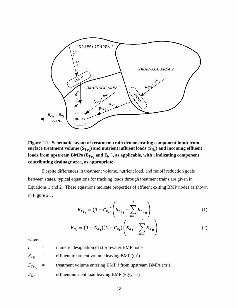
Figure 2.1. Schematic layout of treatment train demonstrating component input from
surface treatment volume (𝐒𝐓𝐕𝐢) and nutrient influent loads (𝐒𝐍𝐢
) and incoming effluent
loads from upstream BMPs (𝐄𝐓𝐕𝐢 and 𝐄𝐍𝐢
), as applicable, with 𝐢 indicating component
contributing drainage area, as appropriate.
Despite differences in treatment volume, nutrient load, and runoff reduction goals
between states, typical equations for tracking loads through treatment trains are given in
Equations 1 and 2. These equations indicate properties of effluent exiting BMP nodes as shown
in Figure 2.1.
𝑬𝑻𝑽𝒊= (𝟏 − 𝑪𝒗𝒊
) (𝑺𝑻𝑽𝒊+ ∑ 𝑬𝑻𝑽𝒖
𝒋
𝒖=𝟎
) (1)
𝑬𝑵𝒊= (𝟏 − 𝑪𝑵𝒊
)(𝟏 − 𝑪𝒗𝒊) (𝑺𝑵𝒊
+ ∑ 𝑬𝑵𝒖
𝒋
𝒖=𝟎
) (2)
where:
𝑖 = numeric designation of stormwater BMP node
𝐸𝑇𝑉𝑖 = effluent treatment volume leaving BMP (m3)
𝐸𝑇𝑉𝑢 = treatment volume entering BMP 𝑖 from upstream BMPs (m3)
𝐸𝑁𝑖 = effluent nutrient load leaving BMP (kg/year)
19
𝐸𝑁𝑢 = nutrient load entering BMP 𝑖 from upstream BMPs (kg/year)
𝐶𝑣𝑖 = credit ratio for reduced volume (static ratio or compute from infiltration rate)
𝐶𝑁𝑖 = credit ratio for nutrient load removals (typically nitrogen or phosphorus)
𝑆𝑇𝑉𝑖 = surface component treatment volume entering BMP (m3)
𝑆𝑁𝑖 = surface component nutrient load entering BMP (kg/year)
∑ 𝑆𝑇𝑉𝑢 = sum of upstream BMP effluent treatment volume entering BMP (m3)
∑ 𝑆𝑁𝑢 = sum of upstream BMP effluent nutrient load entering BMP (kg/year)
𝑗 = number of BMPs upstream from a BMP treatment node
Connectivity and preliminary locations of individual BMP nodes in a treatment train are
typically identified relatively early in the site design process. After logical locations for BMP
nodes are identified, the next step in the design process is compilation of characteristics related
to the contributing drainage area (CDA) of each BMP node. These characteristics include
parameters such as drainage area, land cover conditions, and soil conditions in addition to design
constraints such as the presence of karst features, high groundwater, limited infiltration, and
other constraints that may affect candidate BMP selection by the designer.
Available BMPs can generally be divided into two major categories: proprietary and non-
proprietary BMPs. Proprietary installations can often be the only viable means of treatment in
site re-developments and/or retrofits due to space limitations. Methods of treatment in
proprietary BMPs is through hydrodynamic separation of sediment particles in the runoff,
removal of sediment and pollutants through mechanical filtration, and several others. Non-
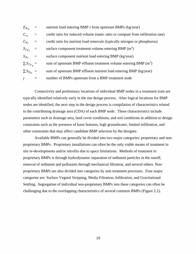
proprietary BMPs are also divided into categories by unit treatment processes. Four major
categories are: Surface Vegetal Stripping, Media Filtration, Infiltration, and Gravitational
Settling. Segregation of individual non-proprietary BMPs into these categories can often be
challenging due to the overlapping characteristics of several common BMPs (Figure 2.2).
20
Figure 2.2. Categorized classifications of non-proprietary stormwater BMPs
At a site scale, the designer’s goal is to reconcile the large number of candidate BMPs
and siting constraints previously discussed, through optimizing a host of competing selection
criteria for each specific project. These selection criteria may include minimization of
installation and maintenance costs, total suspended solids (TSS) load removals above required
reduction, and maximization of parameters such as groundwater recharge, aesthetics, and others,
as warranted by particular project goals. Although the design engineer may be able to rectify
these competing goals on sites where only one or two BMP locations are necessary, larger sites
may require multiple treatment trains consisting of several interconnected BMPs discharging to
multiple drainage outfalls. The number of possible combinations of BMPs can be computed
using standard combinatorial equations. Consider an example site that has ten viable candidate
BMP choices after consideration of physical site constraints (to simplify, it will be assumed that
all CDAs to BMP locations have ten candidates, although on actual projects this number will
likely vary). Table 2.1 summarizes the number of possible combinations to be considered by the
designer for a variety of treatment train scenarios.
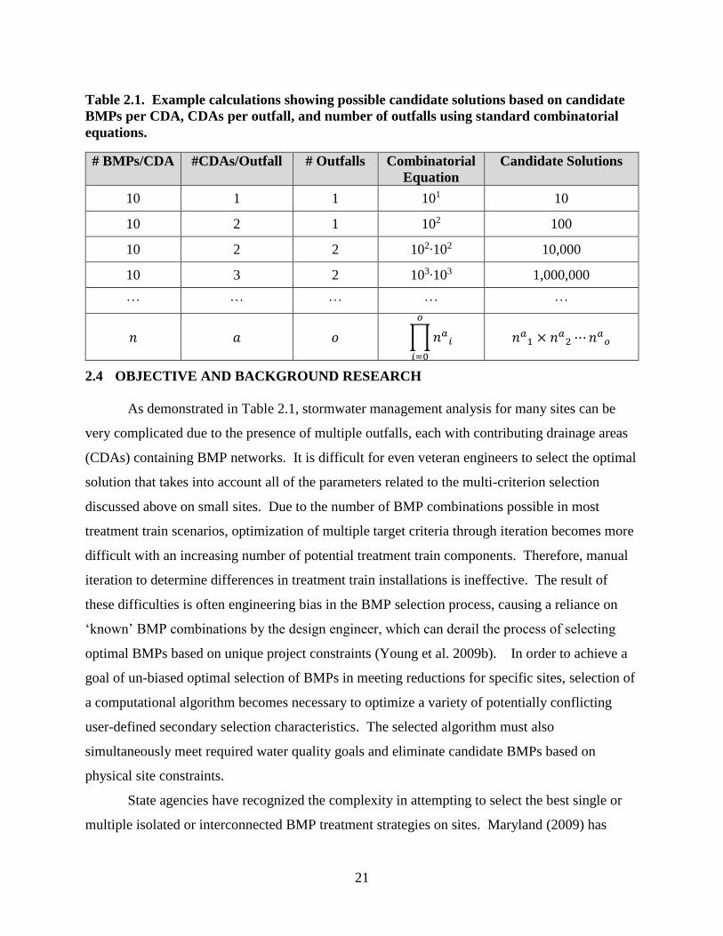
21
Table 2.1. Example calculations showing possible candidate solutions based on candidate
BMPs per CDA, CDAs per outfall, and number of outfalls using standard combinatorial
equations.
# BMPs/CDA #CDAs/Outfall # Outfalls Combinatorial
Equation
Candidate Solutions
10 1 1 101 10
10 2 1 102 100
10 2 2 102∙102 10,000
10 3 2 103∙103 1,000,000
… … … … …
𝑛 𝑎 𝑜 ∏ 𝑛𝑎𝑖
𝑜
𝑖=0
𝑛𝑎1 × 𝑛𝑎
2 ⋯ 𝑛𝑎𝑜
2.4 OBJECTIVE AND BACKGROUND RESEARCH
As demonstrated in Table 2.1, stormwater management analysis for many sites can be
very complicated due to the presence of multiple outfalls, each with contributing drainage areas
(CDAs) containing BMP networks. It is difficult for even veteran engineers to select the optimal
solution that takes into account all of the parameters related to the multi-criterion selection
discussed above on small sites. Due to the number of BMP combinations possible in most
treatment train scenarios, optimization of multiple target criteria through iteration becomes more
difficult with an increasing number of potential treatment train components. Therefore, manual
iteration to determine differences in treatment train installations is ineffective. The result of
these difficulties is often engineering bias in the BMP selection process, causing a reliance on
‘known’ BMP combinations by the design engineer, which can derail the process of selecting
optimal BMPs based on unique project constraints (Young et al. 2009b). In order to achieve a
goal of un-biased optimal selection of BMPs in meeting reductions for specific sites, selection of
a computational algorithm becomes necessary to optimize a variety of potentially conflicting
user-defined secondary selection characteristics. The selected algorithm must also
simultaneously meet required water quality goals and eliminate candidate BMPs based on
physical site constraints.
State agencies have recognized the complexity in attempting to select the best single or
multiple isolated or interconnected BMP treatment strategies on sites. Maryland (2009) has
22
published selection matrices that guide the user through various site constraints to narrow the list
of possible candidate BMPs for use in the stormwater management strategy. Virginia’s
Department of Conservation and Recreation (DCR) attempted to address the issue by
commissioning the Center for Watershed Protection (CWP, 2008) to create a methodology for
estimating the impact of BMPs installed in a distributed network on the site’s runoff
characteristics. The resulting computational process is known as the Virginia Runoff Reduction
Method (VRRM) was adopted May 24, 2011 by the Virginia Soil and Water Conservation
Board. VRRM spreadsheets have provided a compliance tool to aid design engineers in
determining pollutant removal requirements and selecting appropriate BMPs to meet target
removal rates. While this tool does provide a means to determine removal requirements and
methods for compliance, its complexity—especially in the number of entry cells and input
methodology—for testing multiple combinations of BMPs in series, make it prone to input error
and difficult to use iteratively for selecting the best single or group of BMPs based on individual
site characteristics and/or constraints. In addition, the VRRM method requires the user to have
innate knowledge of physical site constraints for each BMP type and provides no avenue for the
user to optimize the solution other than through trial and error. As a compliance tool, the VRRM
spreadsheets, and the VRRM method itself, are limited in scope and do not address stormwater
quantity control regulations, nor do they provide guidance related to final design and sizing of
selected BMPs.
Some jurisdictions have developed software-based tools that generally focus on
narrowing the list of candidate BMPs considered as part of the solution set, but again, do not
focus on an optimized solution. These include the Ohio DOT BMP selection tool (ORIL, 2015),
the Colorado Urban Drainage and Flood Control District UD-BMP (UDFCD, 2010), the White
River Alliance BMP Selection Tool (http://www.ecologik.net/bmpTool/), SWMSoftVA by
Ensoftec (Ensoftec, 2013), BMPSELECT (Pomeroy and Rowney, 2013) and many others.
Other more advanced tools have gone a step further and utilize heuristic algorithms in
order to select and rank BMP selection based on a variety of selection criteria. These include the
Virginia Tech BMP Decision Support Software (Young et al. 2009a), the EPA’s SUSTAIN tool
(U.S. EPA, 2009), and Prince George’s County, Maryland’s BMP-DSS tool (Cheng et al., 2009).
Both the SUSTAIN tool and BMP-DSS (developed by Tetra Tech) are built on top of a Storm
Water Management Model (SWMM) v. 5.0 platform and use a variety of selection factors to
23
ultimately select optimal BMP installations through implementation of scatter search [BMP-DSS
and SUSTAIN] or the Non-dominated Sorting Genetic Algorithm II (NSGA II) [SUSTAIN].
These SWMM oriented tools are tailored to provide feedback on a watershed scale of the most
efficient strategies for meeting various implementation goals, including projected cost. Use of
the SWMM platform allows analysis of BMP treatment trains, and in the case of the SUSTAIN
model, allows optimization algorithms to evaluate various BMP installations within the train.
Both the BMP-DSS and SUSTAIN tools are generally targeted at regional watershed planning.
Individual small-scale project development and BMP optimization on a site scale is not typically
targeted by these tools and use of these tools for such applications is hindered by the large
amount of data and calibration required to get these tools operational. Conversely, the software
tool developed by Virginia Tech (Young et al. 2009a) focuses on BMP selection at the site
development scale. The program uses a list of user selected project constraints and criteria
weightings to provide inputs for Analytic Hierarchy Process (AHP) algorithms, which are then
used to select the highest ranked BMP. Although this provided a significant step forward in the
goal of unbiased selection based on specific project constraints, it does not allow integration of
the selection procedures with distributed treatment train networks nor allow optimization based
on actual nutrient load reduction requirements or runoff reduction which are typically drivers in
BMP selection for project sites.
Liu, et al. (2016) also developed a decision support tool optimally locate stormwater
BMPs and low impact development (LID) practices. The model employs the Multi-Algorithm
Genetically Adaptive Multiobjective (AMALGAM) method to perform multiple parameter
optimization to determine the best locations of various LID and BMP practices at a watershed
scale, with optimization occurring in two stages. The first is within discrete hydrologic response
units (HRUs), and the second is at the watershed scale. Liu et al. (2016) found that optimized
placement of LID and BMP strategies throughout a watershed, rather than random placement,
achieved 3.9 to 7.7 times the runoff and pollutant load reductions at a much lower cost.
Perez-Pedini et al. (2005) and Srivastava et al. (2002) demonstrated that genetic
algorithms can be used when choosing the optimal location of single type infiltration based
BMPs. Integration of NSGA II genetic algorithms in the SUSTAIN tool (U.S. EPA, 2009) has
shown that employing algorithms greatly aids in the selection of candidate BMPs on a watershed
scale. While genetic algorithms have been increasingly used for many engineering optimization
24
problems over the last two decades, selection of the optimal BMP solutions for site scale
development requires reconsideration of viable algorithms for quickly achieving an optimal
solution, which will aid in removing designer bias from the selection process.
2.5 DEVELOPMENT OF OBJECTIVE FUNCTION
Any optimization analysis requires the development of an objective function for
maximization or minimization. The first step in algorithmic implementation includes the
application of rules to narrow the list of candidate BMPs considered during computations. The
logic rules for this pre-processing step are applied regardless of the final optimization algorithm
selected. These rules can include example strategies such as those described in Tables 2.2 and
2.3; however, these are not an exhaustive list of weeding methods that may be applied.
Table 2.2. Example of elimination strategies based on physical constraints in the CDA to
each BMP location.
Physical Constraint Eliminated BMPs
Karst Infiltration type or wetland type BMPs
High Groundwater Any BMP with hampered functionality due to the presence of high
groundwater: Drywells, bioretention, permeable pavement, grass
channels infiltration, extended dry detention
Hotspot Runoff Any BMP which promotes infiltration or direct interaction with
groundwater table: Drywells, bioretention, permeable pavement,
grass channels infiltration, extended dry detention, wet swales (high
groundwater)
Limited/No Infiltration Infiltration type BMPs
Table 2.3. Examples of elimination strategies based on characteristics of CDA to BMP
location.
Parameter Description
Soil Type Eliminates BMP based on specified soil properties.
Contributing
Drainage Area
Eliminates BMPs that are less than the suggested minimum CDA, or
greater than the suggested maximum CDA
Impervious/Turf
Ratio
Eliminate BMPs that are have a CDA with an impervious to turf ratio less
than the suggested minimum or greater than the suggested maximum
Once weeding methods have been applied, the selected algorithm will iterate through
remaining candidate solutions in order to determine the optimal, or an acceptable solution
(depending on algorithm used). It is the method used to reach the solution in the iterative
process that differentiates the various algorithms that may be applied.
25
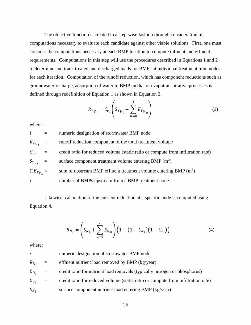
The objective function is created in a step-wise fashion through consideration of
computations necessary to evaluate each candidate against other viable solutions. First, one must
consider the computations necessary at each BMP location to compute influent and effluent
requirements. Computations in this step will use the procedures described in Equations 1 and 2
to determine and track treated and discharged loads for BMPs at individual treatment train nodes
for each iteration. Computation of the runoff reduction, which has component reductions such as
groundwater recharge, adsorption of water to BMP media, or evapotranspirative processes is
defined through redefinition of Equation 1 as shown in Equation 3.
𝑅𝑇𝑉𝑖= 𝐶𝑣𝑖
(𝑆𝑇𝑉𝑖+ ∑ 𝐸𝑇𝑉𝑢
𝑗
𝑢=0
) (3)
where:
𝑖 = numeric designation of stormwater BMP node
𝑅𝑇𝑉𝑖 = runoff reduction component of the total treatment volume
𝐶𝑣𝑖 = credit ratio for reduced volume (static ratio or compute from infiltration rate)
𝑆𝑇𝑉𝑖 = surface component treatment volume entering BMP (m3)
∑ 𝐸𝑇𝑉𝑢 = sum of upstream BMP effluent treatment volume entering BMP (m3)
𝑗 = number of BMPs upstream from a BMP treatment node
Likewise, calculation of the nutrient reduction at a specific node is computed using
Equation 4.
𝑅𝑁𝑖= (𝑆𝑁𝑖
+ ∑ 𝐸𝑁𝑢
𝑗
𝑢=0
) (1 − (1 − 𝐶𝑁𝑖)(1 − 𝐶𝑣𝑖
)) (4)
where:
𝑖 = numeric designation of stormwater BMP node
𝑅𝑁𝑖 = effluent nutrient load removed by BMP (kg/year)
𝐶𝑁𝑖 = credit ratio for nutrient load removals (typically nitrogen or phosphorus)
𝐶𝑣𝑖 = credit ratio for reduced volume (static ratio or compute from infiltration rate)
𝑆𝑁𝑖 = surface component nutrient load entering BMP (kg/year)
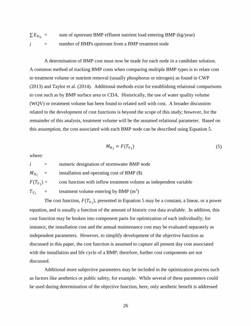
26
∑ 𝐸𝑁𝑢 = sum of upstream BMP effluent nutrient load entering BMP (kg/year)
𝑗 = number of BMPs upstream from a BMP treatment node
A determination of BMP cost must now be made for each node in a candidate solution.
A common method of tracking BMP costs when comparing multiple BMP types is to relate cost
to treatment volume or nutrient removal (usually phosphorus or nitrogen) as found in CWP
(2013) and Taylor et al. (2014). Additional methods exist for establishing relational comparisons
to cost such as by BMP surface area or CDA. Historically, the use of water quality volume
(WQV) or treatment volume has been found to related well with cost. A broader discussion
related to the development of cost functions is beyond the scope of this study; however, for the
remainder of this analysis, treatment volume will be the assumed relational parameter. Based on
this assumption, the cost associated with each BMP node can be described using Equation 5.
𝑀𝑁𝑖= 𝐹(𝑇𝑉𝑖
) (5)
where:
𝑖 = numeric designation of stormwater BMP node
𝑀𝑁𝑖 = installation and operating cost of BMP ($)
𝐹(𝑇𝑉𝑖) = cost function with inflow treatment volume as independent variable
𝑇𝑉𝑖 = treatment volume entering by BMP (m3)
The cost function, 𝐹(𝑇𝑉𝑖), presented in Equation 5 may be a constant, a linear, or a power
equation, and is usually a function of the amount of historic cost data available. In addition, this
cost function may be broken into component parts for optimization of each individually; for
instance, the installation cost and the annual maintenance cost may be evaluated separately as
independent parameters. However, to simplify development of the objective function as
discussed in this paper, the cost function is assumed to capture all present day cost associated
with the installation and life cycle of a BMP; therefore, further cost components are not
discussed.
Additional more subjective parameters may be included in the optimization process such
as factors like aesthetics or public safety, for example. While several of these parameters could
be used during determination of the objective function, here, only aesthetic benefit is addressed
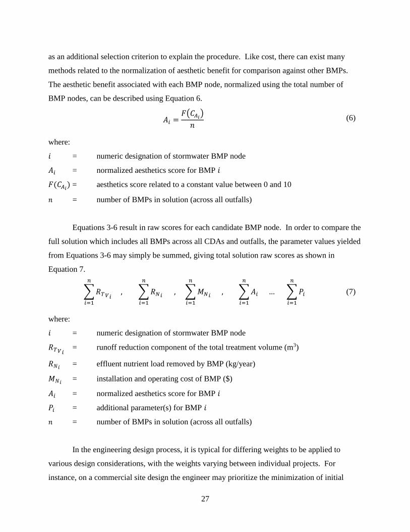
27
as an additional selection criterion to explain the procedure. Like cost, there can exist many
methods related to the normalization of aesthetic benefit for comparison against other BMPs.
The aesthetic benefit associated with each BMP node, normalized using the total number of
BMP nodes, can be described using Equation 6.
𝐴𝑖 =𝐹(𝐶𝐴𝑖
)
𝑛 (6)
where:
𝑖 = numeric designation of stormwater BMP node
𝐴𝑖 = normalized aesthetics score for BMP 𝑖
𝐹(𝐶𝐴𝑖) = aesthetics score related to a constant value between 0 and 10
𝑛 = number of BMPs in solution (across all outfalls)
Equations 3-6 result in raw scores for each candidate BMP node. In order to compare the
full solution which includes all BMPs across all CDAs and outfalls, the parameter values yielded
from Equations 3-6 may simply be summed, giving total solution raw scores as shown in
Equation 7.
∑ 𝑅𝑇𝑉𝑖 , ∑ 𝑅𝑁𝑖
𝑛
𝑖=1
, ∑ 𝑀𝑁𝑖 ,
𝑛
𝑖=1
𝑛
𝑖=1
∑ 𝐴𝑖
𝑛
𝑖=1
… ∑ 𝑃𝑖
𝑛
𝑖=1
(7)
where:
𝑖 = numeric designation of stormwater BMP node
𝑅𝑇𝑉𝑖 = runoff reduction component of the total treatment volume (m3)
𝑅𝑁𝑖 = effluent nutrient load removed by BMP (kg/year)
𝑀𝑁𝑖 = installation and operating cost of BMP ($)
𝐴𝑖 = normalized aesthetics score for BMP 𝑖
𝑃𝑖 = additional parameter(s) for BMP 𝑖
𝑛 = number of BMPs in solution (across all outfalls)
In the engineering design process, it is typical for differing weights to be applied to
various design considerations, with the weights varying between individual projects. For
instance, on a commercial site design the engineer may prioritize the minimization of initial
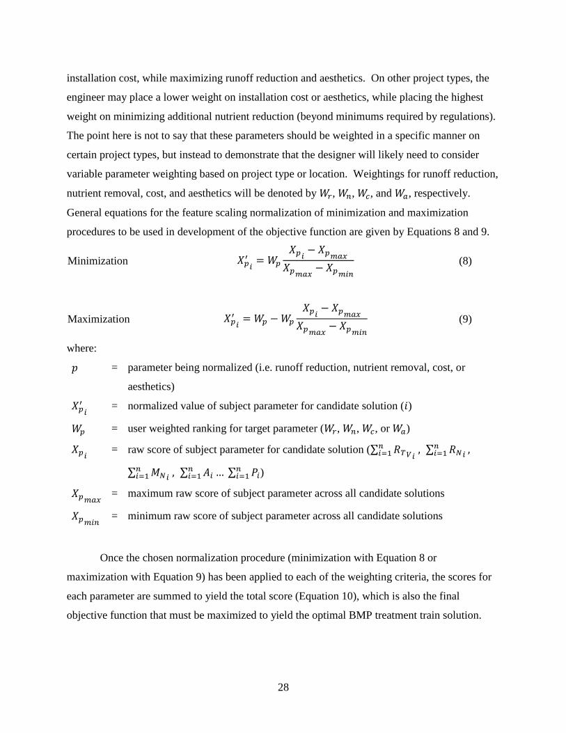
28
installation cost, while maximizing runoff reduction and aesthetics. On other project types, the
engineer may place a lower weight on installation cost or aesthetics, while placing the highest
weight on minimizing additional nutrient reduction (beyond minimums required by regulations).
The point here is not to say that these parameters should be weighted in a specific manner on
certain project types, but instead to demonstrate that the designer will likely need to consider
variable parameter weighting based on project type or location. Weightings for runoff reduction,
nutrient removal, cost, and aesthetics will be denoted by 𝑊𝑟, 𝑊𝑛, 𝑊𝑐, and 𝑊𝑎, respectively.
General equations for the feature scaling normalization of minimization and maximization
procedures to be used in development of the objective function are given by Equations 8 and 9.
Minimization 𝑋𝑝′
𝑖= 𝑊𝑝
𝑋𝑝𝑖− 𝑋𝑝𝑚𝑎𝑥
𝑋𝑝𝑚𝑎𝑥− 𝑋𝑝𝑚𝑖𝑛
(8)
Maximization 𝑋𝑝′
𝑖= 𝑊𝑝 − 𝑊𝑝
𝑋𝑝𝑖− 𝑋𝑝𝑚𝑎𝑥
𝑋𝑝𝑚𝑎𝑥− 𝑋𝑝𝑚𝑖𝑛
(9)
where:
𝑝 = parameter being normalized (i.e. runoff reduction, nutrient removal, cost, or
aesthetics)
𝑋𝑝′
𝑖 = normalized value of subject parameter for candidate solution (𝑖)
𝑊𝑝 = user weighted ranking for target parameter (𝑊𝑟, 𝑊𝑛, 𝑊𝑐, or 𝑊𝑎)
𝑋𝑝𝑖 = raw score of subject parameter for candidate solution (∑ 𝑅𝑇𝑉𝑖
, ∑ 𝑅𝑁𝑖𝑛𝑖=1 ,𝑛
𝑖=1
∑ 𝑀𝑁𝑖 , ∑ 𝐴𝑖
𝑛𝑖=1 … ∑ 𝑃𝑖
𝑛𝑖=1
𝑛𝑖=1 )
𝑋𝑝𝑚𝑎𝑥 = maximum raw score of subject parameter across all candidate solutions
𝑋𝑝𝑚𝑖𝑛 = minimum raw score of subject parameter across all candidate solutions
Once the chosen normalization procedure (minimization with Equation 8 or
maximization with Equation 9) has been applied to each of the weighting criteria, the scores for
each parameter are summed to yield the total score (Equation 10), which is also the final
objective function that must be maximized to yield the optimal BMP treatment train solution.
29
𝑍𝑖 = 𝑋𝑁′
𝑖+ 𝑋𝑅𝑅
′𝑖
+ 𝑋𝐶′
𝑖+ 𝑋𝐴
′𝑖
… 𝑋𝑝′
𝑖 (10)
where:
𝑋𝑁′
𝑖 = Normalized nutrient score for candidate solution (𝑖)
𝑋𝑅𝑅′
𝑖 = Normalized runoff reduction score for candidate solution (𝑖)
𝑋𝐶′
𝑖 = Normalized cost score for candidate solution (𝑖)
𝑋𝐴′
𝑖 = Normalized aesthetics score for candidate solution (𝑖)
𝑋𝑝′
𝑖 = Normalized additional parameter(s) score(s) for candidate solution (𝑖)
𝑍𝑖 = Total raw score for candidate solution (𝑖)
2.6 EVALUATION OF CANDIDATE ALGORITHMS
The optimization problem described above is a discrete nonlinear problem with finite
candidate solutions. In discrete optimization, finite solution combinations are evaluated to
determine the maximum (or minimum) value of the objective function. As described above, with
treatment train connectivity and related CDA geometry draining to each node being static for all
possible solutions, candidate solutions are evaluated by logically iterating through all possible
valid BMP combinations. Because each BMP node type being substituted is defined by discrete
values of runoff and nutrient reduction, all subsequent computations up to development of the
optimization objective function are necessarily discrete.
The selected algorithm to be used for solving this optimization problem, like the
objective function described herein, should meet several potentially conflicting requirements.
1. The algorithm must be able to consistently meet the objective of yielding an optimal
solution.
2. The algorithm must be readily understandable in order to be adopted by a wide array of
practitioners.
3. The algorithm must not be so computationally intensive that normal run times are
excessive.
4. The algorithm must achieve consistently repeatable results between multiple runs.
To achieve these goals, several candidate algorithms were evaluated for use in the
optimization problem based on their past use on problems related to BMP selection and their
ability to meet the criteria listed above.
30
2.6.1 Genetic Algorithms
Genetic algorithms (GA) have been increasingly used in the solution of engineering
optimization problems since proposed by Holland (1975) and brought into the mainstream by
Goldberg (1989). The premise behind GAs is that initial candidate solutions in any generation
(i.e. parents) cross-over with other candidate solutions (mates), generating children solutions (i.e.
offspring) that survive and have the ability to ‘breed’ the next generation based on ‘fitness’.
Additionally, mutations may occur which send computations down new evolutionary branches
that would not be otherwise investigated. Behera and Teegavarapu (2015) used GA based
algorithms to minimize cost associated with installation of detention ponds on single or multiple
parallel watersheds while meeting multi-objective stormwater quality and quantity constraints.
Their dynamic programming (DP) solution through discretization (a simplifying assumption)
was abandoned in favor of genetic algorithms since many of the design variables (e.g.
dimensions of ponds) have solution sets that operate across a continuous range. As described by
Behera and Teegavarapu, using the DP solution for their study would have one of two possible
effects: 1) use of coarse discretization in candidate pond dimensions would potentially yield
results that were not optimal, or 2) decreasing discretization steps would result in increasing
processor time to find the near optimal solution.
U.S. EPA’s (2009) SUSTAIN system attempts to minimize cost against BMP aggregate
sizes based on predefined BMP train options that are tied to upstream land use. The model has
two optimization modes which each use GAs for achieving near optimal solutions (Lee et al.,
2012). The first uses Scatter Search, as described by Lee et al. as sharing some similar
characteristics with GAs. The Scatter Search method is used to solve single-objective problems,
while the second method, NSGA II, is a GA that can be used to solve multi-objective problems.
U.S. EPA (2009) contains a full discussion of the theory behind the two algorithms used for the
SUSTAIN software. The software allows input of predefined BMP train scenarios based on land
use, and then iterates across a continuous range of size and treatment volume scenarios in order
to optimize cost at a watershed scale. Lee et al. (2012) describe two cost optimization functions
that can be chosen within the program, once of which is a cost minimization function providing
near optimal solutions, and the other, a formulation of a cost effectiveness curve.
Perez-Pedini et al. (2005) used GAs to determine the optimal number and location of
infiltration BMPs on a watershed scale. This study focused on the optimization of a single BMP
31
type (infiltration BMPs) throughout the watershed. Since the optimization function used for this
study operates in continuous space (unknown number of BMPs required to meet objective), GA
algorithms are used to find a near optimal solution. Perez-Pedini et al. (2005) discusses
restrictions that were implemented in the decision space to reduce computational time, which
seems to indicate excessive run times for at least some simulations.
As described above, GA solutions have been implemented across a wide range of
engineering problems related to stormwater analysis. Unfortunately, based on analysis of the
predefined algorithmic objectives for this study, implementation of a GA solution does not
appear practical. Behera and Teegavarapu (2015), U.S. EPA (2009) and Perez-Pedini et al.
(2005), discuss that GAs are well suited at finding near optimal solutions in a continuous search
space. The problem described in this study does not exist in a continuous space which would
make application of GAs difficult and hamper the ability to achieve a near-optimal solution that
is reasonably close to the absolute optimal solution. The inability to consistently produce an
optimal solution would also likely impede wide-scale adoption by design professionals. In
addition, GAs can exhibit excessive run times when searching for a near-optimal solution unless
modifications are found that can adjust the run-time as mentioned in Perez-Pedini et al. (2005).
As stated in U.S. EPA (2009), both algorithms used in SUSTAIN incorporate compromises that
result in a near optimal solution by solving across a partially continuous solution set defined by
ranges in sizes of BMPs. This approach is justified by stating that computation of a truly optimal
solution would be extremely time intensive, if at all possible. Excessive run times can be due to
an exponential increase based on input of a large candidate solution pool, or due to the GA
becoming so focused within local maxima (or minima) that genetic cross-over or mutation
cannot dislodge to force movement toward a global optimum.
2.6.2 Analytic Hierarchy Process (AHP)
The AHP is a multi-criteria decision support algorithm that has been used by many
researchers since it was originally proposed by Saaty (1980). Young (2009a, 2009b) integrated
the AHP into a BMP selection decision support tool, and Jato-Espino et al. (2014) integrated the
AHP algorithm in a multi-criteria decision tool to aid in the selection of the appropriate pervious
pavement type for specific projects based on user defined parameters. By default, the AHP is not
an optimization algorithm; however, Javanbarg et al. (2012) extended the abilities of the AHP
through integration of particle swarm optimization (PSO). This PSO extension allows the
32
maximization of the objective function, which pushes the AHP from a support tool to an
integrated optimization tool.
The AHP algorithm operates by deriving a solution vector from evaluation of paired
comparison matrices. For multi-decision optimization, there is typically a pairwise comparison
matrix defining a comparison in weights of selection criteria against all others. In addition, there
is a secondary set of comparison matrices relating distinct parameters for each candidate solution
set. In the case of Young (2009a, 2009b), the candidate matrices compared each candidate BMP
against others at single locations (a single BMP node). For the problem defined in this study, the
comparison matrices would need to describe the relative comparison of one full candidate
solution against another, which can be a single node, but is likely a multi-outfall, multi-node
train configuration. In order to perform these comparisons, static matrices are needed for each
candidate solution. Creation of the comparison matrices, however, requires computation of all
valid solutions prior to generating the pair-wise comparisons. Since all valid solutions must be
computed to create pairwise matrices, use of the AHP process is ultimately unnecessary, because
solution rankings can be computed directly using the candidate configurations in tandem with the
objective function. Therefore, the AHP procedure does not appear to be a good fit for the
optimization problem described in this study since it is tailored to finite decision support models
with a static candidate solution set.
2.6.3 Exhaustive Search
Exhaustive Search (ES) is known by several other names including combinatorial search
and brute force. Fundamentally, the method requires iteration through all possible valid
solutions of the objective function in order to find the optimal solution, although intelligence
functions can be added to logically decrease the candidate solution set. These adaptations
provide the key to addressing excessive run times, a common issue that can hamper use of this
algorithm on many optimization problems. Rao (2009), notes that exhaustive search is well-
suited for finding the optimal solution for an objective function that operates in a finite solution
space. Several key characteristics that sets the ES algorithm apart from the GA algorithms is that
given enough time, the ES algorithm will find the optimal solution, it is understandable, and run
times can be kept to minimal levels if enough pre-processing (weeding) takes place.
Although the validity of solutions produced by ES are above reproach since all solutions
are explored, Nievergelt (2000) states that in many academic circles, use of the ES algorithm is

33
considered ‘inelegant’. Nievergelt (2000) also explains that due to dramatic increases in
processing power that interest in the ES approach has been renewed and the technique has been
applied to ‘messy’ problems that are difficult to solve using more ‘elegant’ approaches, such as
with genetic algorithms. Use of an ES algorithm appears to be well adapted to maximizing the
objective function described in this study; however, prior to selection, the primary weakness
plaguing ES algorithms must be addressed—computational run times.
To definitively quantify run times, an ES algorithm using the Virginia Runoff Reduction
Method (VRRM) was implemented to iterate through BMP solutions over multiple outfalls and
multi-level treatment trains in order to validate the approximate time necessary for various levels
of computation. Since the algorithm is being applied at the site scale and not the watershed or
regional scale as with other studies such as U.S. EPA (2009) and Perez-Pedeni (2005), the total
number of combinatorial outcomes is expected to be less than 1,000,000, similar to scenario four
in Table 2.1, on projects with small land disturbances, which would likely keep runtimes to
manageable levels (1 second – 5 minutes). This expectation is based on analysis of
representative ranges in size of land disturbance projects in Virginia by computing representative
statistics for active Virginia Stormwater Management Permit (VSMP) holders (VDEQ, 2016)
across the Commonwealth of Virginia. Figure 2.3 provides a statistical distribution of the 5,187
active development projects in Virginia in March 2016. As shown in Figure 2.3, 95% of all
development projects within the Commonwealth are 30 hectares or less, with 75% being 6
hectares or less. Based on this data, it can be assumed that the majority of projects will have
limited numbers outfalls, CDAs, and treatment train configurations, and are likely to fall within
the combinatorial example ranges that are presented in Table 2.1, with few exceptions.
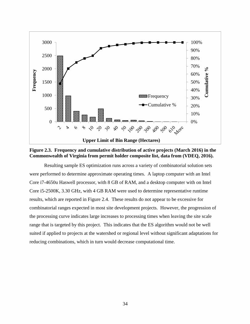
34
Figure 2.3. Frequency and cumulative distribution of active projects (March 2016) in the
Commonwealth of Virginia from permit holder composite list, data from (VDEQ, 2016).
Resulting sample ES optimization runs across a variety of combinatorial solution sets
were performed to determine approximate operating times. A laptop computer with an Intel
Core i7-4650u Haswell processor, with 8 GB of RAM, and a desktop computer with on Intel
Core i5-2500K, 3.30 GHz, with 4 GB RAM were used to determine representative runtime
results, which are reported in Figure 2.4. These results do not appear to be excessive for
combinatorial ranges expected in most site development projects. However, the progression of
the processing curve indicates large increases to processing times when leaving the site scale
range that is targeted by this project. This indicates that the ES algorithm would not be well
suited if applied to projects at the watershed or regional level without significant adaptations for
reducing combinations, which in turn would decrease computational time.
0%
10%
20%
30%
40%
50%
60%
70%
80%
90%
100%
0
500
1000
1500
2000
2500
3000
Cu
mu
lati
ve
%
Fre
qu
ency
Upper Limit of Bin Range (Hectares)
Frequency
Cumulative %
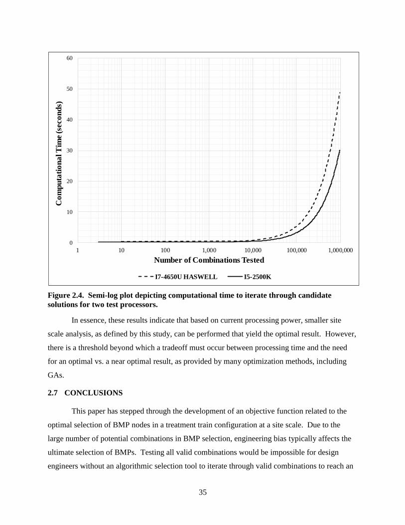
35
Figure 2.4. Semi-log plot depicting computational time to iterate through candidate
solutions for two test processors.
In essence, these results indicate that based on current processing power, smaller site
scale analysis, as defined by this study, can be performed that yield the optimal result. However,
there is a threshold beyond which a tradeoff must occur between processing time and the need
for an optimal vs. a near optimal result, as provided by many optimization methods, including
GAs.
2.7 CONCLUSIONS
This paper has stepped through the development of an objective function related to the
optimal selection of BMP nodes in a treatment train configuration at a site scale. Due to the
large number of potential combinations in BMP selection, engineering bias typically affects the
ultimate selection of BMPs. Testing all valid combinations would be impossible for design
engineers without an algorithmic selection tool to iterate through valid combinations to reach an
0
10
20
30
40
50
60
1 10 100 1,000 10,000 100,000 1,000,000
Co
mp
uta
tio
na
l T
ime (se
co
nd
s)
Number of Combinations Tested
I7-4650U HASWELL I5-2500K
36
optimal solution for many sites. Based on a review of the literature, three possible candidate
algorithms were considered for implementation in a tool used to optimally evaluate the objective
function defined in this study.
Of the three evaluated algorithms in this study, based on analysis of solution space, the
objective function, and defined algorithmic selection goals, the exhaustive search method is the
only candidate solution algorithm that meets all of the stated objectives. For discrete
optimization problems, ES algorithms will find the optimal solution, are easy to understand, and
results are identical between successive program runs since all valid solutions are evaluated.
Ultimately, processing speed is specific to computer hardware and is difficult to evaluate without
application of the ES algorithm to the objective function described by this study. However,
preprocessing by weeding illogical candidates, user defined constraints, and designer based
omission of illogical BMPs at each BMP node will reduce the possibility of an excessive
candidate solution set, and thus, run times. Tests using two computers that are representative of
those used by design engineers indicate similar processing times throughout the range of
combinatorial solutions tested. Those tests also indicate that the algorithm discussed in this
paper should only be applied to projects at a site scale due to the likelihood of dramatically
increased run times at a regional level. For watershed level or regional analysis, it is likely that
GAs or other non-optimal solutions, such as those methods proposed in Behera and Teegavarapu
(2015), Lee et al. (2012), Perez-Pedini et al. (2005), or Liu et al. (2016) would be necessary to
determine an acceptable non-optimal solution in order to reduce computational time.
The problem described in this study exists in a finite (discrete) search space and seeks to
find the optimal solution, which does not promote the use of GAs or similar algorithms that are
more effective for continuous solution sets. Though the AHP process has been applied to
decision support tools related to BMP selection in the past, its use of comparison matrices does
not promote rapid integration or viability for use for optimization of the objective function
described herein. It is believed that a tool developed using the ES algorithm for BMP selection
will be a tremendous benefit to the design community at large by providing and easy to
understand, reproducible, and rapid method for determining the optimal layout of BMPs in a
treatment train configuration.

37
2.8 ACKNOWLEDGEMENTS
Author contributions: C. Hodges and R. Dymond wrote the journal article, formulated
the objective function, and evaluated advantages/disadvantages of potential algorithms. C.
Hodges developed a computational model to evaluate the ES algorithm and computed run times
for various scenarios. Other contributions: Kevin D. Young, Virginia Tech provided peer
reviews of algorithm selection and evaluation of results, which was invaluable due to his
previous work in the field.
38
2.9 REFERENCES
Balascio, C. and Lucas, W. (2009). “A survey of storm-water management water quality
regulations in four Mid-Atlantic States.” Journal of Environmental Management. 90(1),
1-7.
Behera, P. and Teegavarapu, R. (2015). “Optimization of a Stormwater Quality Management
Pond System.” Water Resources Management. 29(4), 1083-1095.
Center for Watershed Protection (CWP) (2008). “Technical Memorandum: The Runoff
Reduction Method.”
<http://www.vwrrc.vt.edu/swc/documents/CWP_TechMemo_VRRM_20080418.>
(October 12, 2015)
Center for Watershed Protection (CWP) (2013). “Cost-Effectiveness Study of Urban Stormwater
BMPs in the James River Basin.” Ellicott City, MD.
<http://www.jamesriverassociation.org/what-we-do/JRA-Cost-effective-Full-Report-
June-update.pdf> (March 21, 2016)
Cheng, M.S., Zhen, J.X., Shoemaker, L. (2009). “BMP decision support system for evaluating
stormwater management alternatives.” Front. Environ. Sci. Eng. China, pp. 453–463.
Clarke, J. (2003). “Clean Water Act. Water: Science and Issues.”
<http://www.encyclopedia.com/doc/1G2-3409400062.html> (October 12, 2015)
Elliott, A.H. and Trowsdale, S.A. (2007). “A review of models for low impact urban stormwater
drainage.” Environmental Modelling and Software. (22), 394-405.
Ensoftec, (2013). SWMSoftVA, v 1.0. < https://www.ensoftec.com/ > (January 6, 2016).
Goldberg, D. E. (1989). “Genetic algorithms in search, optimization, and machine learning.”
Reading, MA: Addison-Wesley.
Holland, J.H. (1975). “Adaptation in Natural and Artificial Systems.” University of Michigan
Press.
Jato-Espino, D., Rodriguez-Hernandez, J. Andrés-Valeri, V., Ballester-Muñoz, F. (2014). “A
fuzzy stochastic multi-criteria model for the selection of urban pervious pavements.”
Expert systems with applications. 41(15), 6807. DOI: 10.1016/j.eswa.2014.05.008
Javanbarg, M., Scawthorn, C., Kiyono, J., and Shahbodaghkhan, B. (2012). “Fuzzy AHP-based
multicriteria decision making systems using particle swarm optimization.” Expert
Systems with Applications: An International Journal 39(1), 960-966.
Lee, J.G., Selakumar, A., Alvi, K., Riverson, J., Zhen, J., Shoemaker, L., and Lai, F. (2012). “A
watershed-scale design optimization model for stormwater best management practices.”
Environmental Modelling & Software. (37), 6-18.
39
Li, H., Sharkey, L., Hunt, W., and Davis, A. (2009). “Mitigation of Impervious Surface
Hydrology Using Bioretention in North Carolina and Maryland.” Journal of Hydrologic
Engineering. 14(4), 407-415.
Liu, Y., Cibin, R., Bralts, V., Chaubey, I., Bowling, L., and Engel, B. (2016). “Optimal selection
and placement of BMPs and LID practices with a rainfall-runoff model.” Environmental
Modelling & Software. (80), 281-296.
Maryland Department of the Environment Water Management Administration and Center for
Watershed Protection (2009). “2000 Maryland Stormwater Design Manual.”
<http://www.mde.state.md.us/programs/water/stormwatermanagementprogram/maryland
stormwaterdesignmanual/Pages/Programs/WaterPrograms/SedimentandStormwater/stor
mwater_design/index.aspx.> (September 25, 2015)
Nievergelt, J. (2000). “Exhaustive search, combinatorial optimization and enumeration:
Exploring the potential of raw computing power.” In Sofsem 2000: theory and practice of
informatics. 18-35. Springer Berlin Heidelberg.
North Carolina Department of Environmental and Natural Resources (NCDENR) (2007).
“Stormwater BMP Manual.” <http://portal.ncdenr.org/web/lr/bmp-manual.> (September
25, 2015).
Ohio's Research Initiative for Locals (ORIL) (2015). “Stormwater BMP Selection Tool for Local
Roadways.”
<https://www.dot.state.oh.us/groups/oril/Documents/Projects/134990_ORIL7_BMPtool_
Final_Locked_0.xlsx.> (September 27, 2015).
Pennsylvania Department of Environmental Protection (PADEP) (2006). “Pennsylvania
Stormwater BMP Manual.” Doc: 363-0300-002.
<http://www.elibrary.dep.state.pa.us/dsweb/Get/Document-68851/363-0300-002.pdf.>
(September 25, 2015).
Perez-Pedini, C., Limbrunner, J.F., and Vogel, R.M. (2005). “Optimal location of infiltration-
based best management practices for storm water management.” Journal of Water
Resources Planning and Management 131(6), 441-448.
Pomeroy, C.A. and Rowney, A. C. (2013). “User’s Guide to the BMP SELECT Model.” Water
Environment Research Foundation, Alexandria, Virginia, SWC1R06c.
Rao, Signgiresu (2009). “Engineering Optimization: Theory and Practice.” John Wiley & Sons,
p.256.
Saaty, T.L. (1980). “The Analytic Hierarchy Process.” McGraw-Hill, New York.
Shuster, W., Gehring, R., and Gerken, J. (2007). “Prospects for enhanced groundwater recharge
via infiltration of urban storm water runoff: A case study.” Journal of Soil and Water
Conservation. 62(3), 129-137.
40
Srivastava, P., Hamlett, J.M., Robillard, P.D. and Day, R.L. (2002). “Watershed optimization of
best management practices using AnnAGNPS and a genetic algorithm.” Water Resources
Research, 38(3).
Taylor, S., Barrett, M., Leisenring, M., Sahu, S., Pankani, D., Poresky, A., Questad, A., Strecker,
E., Weinstein, N., and Venner, M. (2014). “Long-Term Performance and Life-Cycle
Costs of Stormwater Best Management Practices.” Transportation Research Board of the
National Academies, Washington, DC.
Urban Drainage and Flood Control District (UDFCD) (2010). “Urban Storm Drainage Criteria
Manual Volume 3, Best Management Practices.” Water Resources Publications, LLC.
Denver, Colorado.
United States Environmental Protection Agency (2009). “SUSTAIN – A Framework for
Placement of Best Management Practices in Urban Watersheds to Protect Water
Quality.” Publication No. EPA/600/R-09/095. September 2009.
Virginia Department of Environmental Quality (VDEQ) (2013). “Virginia Stormwater
Management Handbook, 2nd Edition, Draft.”
<http://www.deq.virginia.gov/fileshare/wps/2013_SWM_Handbook/.> (September 25,
2015).
Virginia Department of Environmental Quality (VDEQ) (2016). “List of Active Construction
General Permits.”
<http://www.deq.virginia.gov/Portals/0/DEQ/Water/StormwaterManagement/2014_CGP
_ACTIVE_WEB.xlsx> (March 18, 2016).
West Virginia Department of Environmental Protection (WVDEP) (2012). “West Virginia
Stormwater Management and Design Guidance Manual.”
<http://www.dep.wv.gov/WWE/Programs/stormwater/MS4/Pages/StormwaterManageme
ntDesignandGuidanceManual.aspx.> (September 25, 2015).
Young, K. D., Younos, T., Dymond, R. L., and Kibler, D. F. (2009a). “Virginia’s Stormwater
Impact Evaluation: Developing an Optimization Tool for Improved Site Development,
Selection and Placement of Stormwater Runoff BMPs.” VWRRC SR44-2009, Virginia
Tech, Blacksburg, VA.
Young, K., Kibler, D., Benham, B., and Loganathan, G. (2009b). “Application of the Analytical
Hierarchical Process for Improved Selection of Storm-Water BMPs.” Journal of Water
Resources Planning and Management. 135(4), 264-275.
41
Chapter 3: Generation of Cost Functions for use in Stormwater BMP
Selection Optimization
Hodges, C.C.1, Dymond, R.L.2, Young, K.D.3
Status: This manuscript was submitted to ASCE Journal of Sustainable Water in the Built
Environment in May 2016 and is in review.
3.1 ABSTRACT
During selection of optimal series of stormwater BMPs for a development site, designers
must simultaneously consider multiple competing criteria for final selection, one of which is
typically cost. A review of previous studies related to capital and O&M costs for various
stormwater BMPs is conducted with the goal of developing a methodology for creating cost
functions for integration in a BMP selection optimization algorithm. Four methods for relating
cost to various BMP parameters are considered prior to selecting treatment volume as the best
alternative. The selected method is applied to a wide array of non-proprietary structural BMP
practices within the Commonwealth of Virginia to produce capital cost functions for all BMPs as
related to treatment volume. The selected method for estimation of maintenance cost is based on
a percentage of construction cost, with recommended values established from an analysis of
previous studies.
1 Graduate Research Assistant, Via Department of Civil and Environmental Engineering,
Virginia Tech, 200 Patton Hall, Blacksburg, VA 24061 (e-mail: [email protected]) 2 Associate Professor, Via Department of Civil and Environmental Engineering, Virginia Tech,
200 Patton Hall, Blacksburg, VA 24061 (e-mail: [email protected]) 3 Professor of Practice, Via Department of Civil and Environmental Engineering, Virginia Tech,
200 Patton Hall, Blacksburg, VA 24061 (e-mail: [email protected])
42
3.2 INTRODUCTION
During the middle to late 20th century, stormwater management related to site
development projects generally focused on prevention of flooding downstream, and to a more
limited extent, erosion control. Historically, flood control has been managed using
impoundments which temporarily store an excessive volume of runoff to release to the receiving
stream at a controlled rate. In addition to decreasing the peak runoff rate into receiving streams,
temporary impoundment promotes partial settling of the suspended sediment load within the
treatment volume. This method of management may be cost effective to implement on a site;
however, since it does not address higher runoff volumes generated by land development
activities, downstream degradation can occur which can cause regional economic and
environmental impacts.
After passage of the Clean Water Act (33 U.S.C §1251 et seq., 1972) and its
amendments, including the Water Quality Act (1987), the United States Environment Protection
Agency (USEPA) was tasked with oversight of the National Pollutant Discharge Elimination
System (NPDES) program and resulting permits in an effort to improve the quality of the
nation’s waters through the establishment of various allowable target thresholds of sediment,
nutrients, and environmental toxins. The 1990 NPDES Stormwater Permit program hinged on
redefinition of stormwater discharges from Municipal Separate Storm Sewer Systems (MS4s) as
point source discharges (USEPA, 2016), causing them to fall under the purview of the NPDES
permit program. Roll out of the NPDES stormwater permit program was phased, with permits
required first in 1990 by Phase I communities (populations exceeding 100,000), and later,
starting in 1999, by Phase II (USEPA, 2005) communities (populations between 50,000 and
100,000, with lower thresholds depending on several designation criteria such as discharge to
impaired waters, population density, etc.).
Integration of water quality requirements through the NPDES program resulted in a
paradigm shift in site scale stormwater management. It is now accepted that the most effective
way to reduce degradation in receiving streams is by mimicking predevelopment hydrologic
characteristics on the developed site. Because traditional stormwater impoundments are not
effective at replicating predevelopment hydrologic characteristics, stormwater runoff is now
commonly treated in relatively small scale stormwater BMPs distributed throughout the site in an
attempt to maximize volume, nutrient, and sediment load reductions. Often, these distributed
43
BMPs are interconnected to allow secondary and tertiary treatment, in networks colloquially
referred to as ‘treatment trains’. Treatment through these BMPs has benefits to receiving waters,
including, reduction in downstream erosion, nutrient and toxin loads to receiving streams
(Schueler and Youngk, 2015), and partial mitigation of thermal impacts caused by development
(Long and Dymond, 2013).
In practice, manual optimization when integrating treatment trains in the design process
can be difficult due to the need to simultaneously consider regulatory requirements against
competing physical site constraints (Young et al., 2011) and cost. This is compounded with
increasing site size and number of outfalls, where the number of viable solution combinations
can be in the thousands. Due to the inability to test every viable candidate train for
determination of the optimal solution, bias can creep into the design process. To maintain
objectivity in the selection process, software based optimization can be employed for optimal
treatment train selection. Past stormwater BMP optimization efforts on a regional or watershed
scale have maximized nutrient removal and/or volume reduction, while minimizing cost (Cheng
et al., 2006, USEPA, 2011). For land development projects, the regulatory requirements for
pollutant or volume load computation, as well as efficiencies related to discharge efficiencies are
typically established by state or local legislation, including a regulatory method for computation.
Therefore, inclusion of pollutant/nutrient loadings and removal efficiencies in the maximization
(load/volume reduction) portion of the selection algorithm must be employed based on local/state
standards without regard to efficacy.
Cost functions, however, are dynamic and based largely on market conditions, and unlike
regulatory pollutant removals, are not mandated values. Creation of functions for cost
minimization initially seems to be a relatively easy task; however, reliable estimates of
stormwater BMP costs are difficult to produce due to regional variation in labor and material
costs, inflation, seasonal variation in material costs, lack of consistency in design standards and
construction practices in historic BMP cost databases, the large variety of stormwater BMPs, and
many other factors. Although many states (North Carolina, 2007; Maryland, 2009; West
Virginia, 2012; Pennsylvania, 2006; Virginia, 2013) have defined specific efficiencies related to
pollutant, nutrient, and volume reductions to BMP types, few have provided specific guidance on
cost implications of the various practices, instead relying heavily on studies such as that by
USEPA (1999) to provide an indication of cost.
44
This study focuses on development of a standard methodology to provide expected
construction and maintenance cost functions, for integration in an optimization algorithm for
optimal selection of BMP treatment train components against competing alternatives. A
complete BMP cost is determined through compilation of various component costs. These can
include design costs, construction (capital) costs, operating and maintenance (O&M) costs, and
end of life disposal and replacement costs. Design costs are not considered for this study, as it is
assumed that the magnitude of design costs is similar between all BMP categories for a specific
site. Construction cost, though the focus of most engineering cost opinions, may not be the
primary cost consideration in the life cycle of treatment BMPs, since O&M costs are high for
many practices. Various studies have attempted to define construction and O&M costs as
described in later sections. Although disposal and end of life replacement costs rival initial
installation costs, there is little present data on the life expectancy of most BMPs, which hampers
integration of end of life costs in net present value (NPV) or annualized estimations of cost;
therefore, these costs are not included in this study.
3.3 REVIEW OF LITERATURE
USEPA (1999) was, at the time, a pivotal report on the state of the practice of BMP
technology. This report consolidated nutrient efficiency, runoff reduction, cost data, etc. related
to stormwater BMPs, which included the newer BMP implemented in Phase I communities over
the previous decade. The construction cost data summarized in the report was based on studies
by Brown and Schueler (1997) or SWRPC (1991). Construction cost functions provided for
BMPs investigated by USEPA (1999) are related to volume for storage type BMPs (detention,
retention, and infiltration) and surface treatment area for porous pavements, filter strips, and
grassed channels. Sand filters were separately correlated to the impervious component of the
contributing drainage area (CDA). USEPA (1999) was groundbreaking in providing direction
for creation of BMP cost estimates; however, the varying normalization parameters used for
developing construction cost functions between BMP categories hampers rapid comparison
between competing BMP types during selection. Annual maintenance cost, as reported by
USEPA (1999) was generally reported as a percentage of BMP construction cost, and based on a
consolidation of various studies by Wiegand et al. (1986), Schueler (1987), SWRPC (1991),
Livingston et al. (1997), and Brown and Schueler (1997).
45
Water Environment Research Foundation (WERF, 2005) produced a report summarizing
performance and whole life cost of stormwater BMPS. The study was undertaken in an effort to
overcome several deficiencies related to cost analysis of BMPs, including lack of historic cost
and operational data and little understanding of long-term liabilities associated with BMP
installations. Authors of the study noted significant regional discrepancies in cost and
maintenance between similar BMP types that were largely attributed to local perceptions or
regulations regarding aesthetics of installed practices. The WERF model evaluates various
installation and operational costs (capital, operating and maintenance (O&M), monitoring,
disposal, residual, and others) related to BMPs to determine a NPV whole life cost. WERF
(2005) noted several deficiencies with its developed methodology, including limited data
availability for generation of costs and the extreme sensitivity of whole life cost to the associated
maintenance cost component.
The authors of WERF (2005) noted that computation of installation costs would not
benefit from a national effort in compiling installation costs by BMP types. Instead, capital cost
functions should be generated locally based either on local installation cost data, or local
engineering cost opinions that effectively take into account regional variations in labor and
material costs. Capital cost functions generated by WERF (2005) are related to physical size of
the facility and vary by type, with ponding categories related to volume (m3),
infiltration/filtration beds related to area (m2), and linear practices such as grass swales related to
distance (m). Operation and maintenance costs in the study are defined as a percentage of the
capital construction cost, similar to USEPA (1999). The data and cost curves generated from
WERF (2005) are the basis for the cost analysis that is included in the WERF SELECT BMP
selection spreadsheet tool (WERF, 2013).
Weiss et al. (2007) performed an analysis of six types of stormwater BMPs to determine
both construction and O&M costs with the goal of developing a tool for comparison of
stormwater BMPS. The study defined the total present cost as capital cost plus the NPV of an
additional twenty years of O&M costs. Regional cost adjustment factors as published by the
USEPA (1999) were used to convert national cost data to a common basis. Weiss et al. (2007)
determined that data compared using the water quality volume (WQV) of BMPs produces less
scatter when plotted than that related to CDA. A review of current data at the time of the study
was performed in an attempt to statistically analyze O&M costs for various BMPs; however, no
46
historical O&M data was found for any of the BMP types. Due to the reported lack of historic
O&M cost data, Weiss et al. recommend estimating the costs as a percentage of construction
cost, and reference those reported in USEPA (1999) as well as reporting values from additional
studies in the literature (SWRPC,1991; Landphair et al., 2000; Caltrans, 2004; Moran and Hunt,
2004).
USEPA SUSTAIN (Shoemaker et al., 2009) was developed as a decision support tool to
aid planners in developing and optimizing regional stormwater management plans. Subsequent
updates have been performed, resulting in the most recent version, released June 2014 (USEPA,
2014). The software uses genetic algorithms to select locations and estimate costs by attempting
to simultaneously maximize pollutant and volume removal, while minimizing cost. The authors
note extreme sensitivity in model results to BMP cost data. Construction cost data used for
computations in SUSTAIN come from a variety of sources including wholesale retail costs, EPA
Stormwater Fact Sheets (932-F-99-001 to 048), the California Department of Transportation
(CALTRANS), Fairfax County, Virginia, BMP Fact sheets, Natural Resources Conservation
Service (NRCS) Cost Share Data, and several others. SUSTAIN (USEPA, 2014), relies heavily
on NRCS cost share data for development of cost curves, which the authors state is focused
primarily on agricultural or rural projects, with few costs based on urban applications.
The Minnesota Pollution Control Agency (MPCA, 2011) commissioned a report detailing
construction and maintenance costs for stormwater BMPs. Capital costs were consolidated from
actual construction cost data, converted to NPV 2010, and related to the treatment WQV of each
BMP. The treatment WQV, as defined in the report, is not a design volume based on
characteristics of the CDA and precipitation data. Instead, it is defined as the storage volume
below the overflow for some filtration/infiltration practices, eighteen inches over the surface area
for wetland type BMPs or the dead storage volume for extended detention facilities. Linear grass
swales were omitted from analysis due to insufficient data available to estimate an as-constructed
WQV.
Colorado State University, the Urban Watersheds Research Institute, and the Colorado
Urban Drainage Flood Control District have developed a spreadsheet tool, Best Management
Practices – Rational Estimation of Actual Likely Costs of Stormwater Treatment (BMP –
REALCOST) to aid in the estimation of construction costs of stormwater BMPs in the Denver
metropolitan area (Olson et al., 2013). As reported by Olson et al. (2013), the tool uses data
47
from engineering cost opinions created and statistically analyzed for creation of cost curves
related to various BMP categories. Resulting cost functions relate probable construction cost to
the contributing impervious area. The basis of the analysis was development of conceptual
designs of the various BMP types across the expected operational range (i.e., contributing
drainage areas, impervious cover, etc.) for each. The designers note that the developed curves
are “approximate and intended primarily for comparative purposes” (Olson et al., 2013).
Additionally, the authors warn that since the curves were developed across operational
contributing drainage area (CDA) ranges, and not nutrient/pollutant removal ranges, that each
cost function does not “in itself reveal the relative treatment costs per pound of pollutant
removed.”
The Center for Watershed Protection (CWP, 2013) prepared a study at the request of the
James River Foundation (JRF, Virginia) to evaluate cost-effectiveness of various urban
stormwater BMPs. The study defines cost-effectiveness in terms of annualized life cycle costs
per pound of pollutant removed. This study is novel in that it suggests normalization using
nutrient removal as a standard metric across all BMP categories, which addressed a shortcoming
in the study by Olson et al. (2013). Although the study did not focus on selection of BMPs, a
variation of the standard employed for comparing cost to nutrient removal appears well suited to
the task.
The International Stormwater BMP Database [ISBMPD] (2014) is a compendium of
studies related to BMP installation, performance, and cost. Started in 1996 as a joint project by
the American Society of Civil Engineers (ASCE) and USEPA, the project more recently added
new partners including WERF, the Federal Highway Administration (FHWA), the American
Public Works Association (APWA) and the Environmental and Water Resources Institute
(EWRI). Updated every several years, the 2014 version of the database holds 145 records
related to BMP cost. The data reported by ISBMPD (2014) related to cost is often inconsistent,
and contains incomplete records. For instance, of the 145 records related to cost, only 49 list the
initial construction cost, with only 9 of those records occurring after year 2000, around the time
Phase II MS4s began installation of water quality BMPs. With little information given by
ISBMPD (2014) related to construction and design specifications for BMPs, and the small
number of recent construction cost records overall, there is insufficient data related to
construction costs for the newer generation of stormwater BMPs to provide a statistically valid
48
sample for analysis in the determination of cost. In addition, ISBMPD (2014) has no records
related to the O&M costs of reported installations.
The National Cooperative Highway Research Program (NCHRP) published a 2014 report
(Taylor et al., 2014) aimed at aiding the designer in optimization of the stormwater BMP design
and maintenance, primarily for Department of Transportation (DOT) programs. To date, it is
one of the most comprehensive studies of the type, using not only data from past studies, but also
collecting cost and performance data directly from transportation programs in all states. The
study produced a report as well as spreadsheets for various BMP types to aid in computation of
whole life cycle costs. Like CWP (2013), costs between BMP types were related to removal of
various nutrients and pollutants, including E. Coli, fecal coliform, total copper, total lead, total
zinc, nitrate, total Kjeldahl nitrogen, total nitrogen, dissolved phosphorus, total phosphorus, and
total suspended solids. Construction cost data was developed using unit costs (RS Means
publications) along with estimated units of materials as input by the user. O&M cost estimates,
unlike most previous studies, do not correlate maintenance costs as a percentage of construction
cost, but instead uses results from statistical analysis of collected data regarding maintenance
hours (labor) and equipment and material cost from various DOT project studies. Taylor et al.
(2014) also expands on previous work by attempting to provide a whole life cycle cost
calculation by predicting full future replacement of BMPs based on likely life expectancy of
major BMP components. A shortcoming of the study, as related to new site development
projects, as explained in Taylor et al. (2014), is that the cost information is specifically tied to
retrofit of existing stormwater infrastructure on highway projects. The authors suggest that
designers using the developed spreadsheets on new projects would need to override supplied unit
cost data and local performance metrics prior to utilizing the tool.
3.4 METHODOLOGY
The goal of this project is to develop a consistent method for development of cost
functions for both construction and maintenance costs that may be used in a site scale BMP
selection optimization tool. Because the primary focus of the tool will be comparison between
BMP treatment train solutions, and not as a cost estimation tool, the absolute accuracy of the
determined cost is less important than a realistic relative cost between candidate solutions. A
review of the literature has indicated generalized guidance in the development of both
49
construction and maintenance cost functions. As indicated by Taylor et al. (2014), Olson et al.
(2013), Shoemaker et al. (2009), and WERF (2005), regional variations in initial construction
costs of stormwater BMPs should be addressed through the creation of cost functions either by
using historic local materials and labor data, or locally created engineering cost opinions. Most
studies found in the literature (USEPA, 1999; Weiss et al., 2007; MPCA, 2011; King and Hagan,
2011) define operating and maintenance cost as a percentage of initial installation cost.
Therefore, this study follows recommendations in the literature and bases initial construction
cost functions on locally based unit component costs for stormwater BMPs. O&M cost is
computed as a percentage of initial construction cost, as indicated by a review of the literature.
3.4.1 Evaluation of BMP Design Parameters vs. Cost
Attempts to provide objective relative cost comparisons between BMPs has resulted in a
variety of relational methods that can be used to estimate BMP construction and maintenance
costs. Past studies have indicated four distinct parameters typically relating construction and/or
maintenance costs of stormwater BMPs. These include costs related to:
Water quality volume (WQV)
Contributing Drainage Area (or impervious portion of CDA)
BMP size (length, area, or volume)
Nutrient or pollutant removal
Each of these parameters were evaluated for integration in cost functions to be used in an
algorithm for selection of the optimal layout of distributed stormwater BMPs at the site scale.
3.4.1.1 Water Quality Volume
WQV, is a standard metric that is commonly used to determine sizing for selected
stormwater BMPs. The volume is sometimes based on a rainfall depth over the impervious
portion of the CDA, but also can be based on a depth over the entire CDA with adjustments to
account for pervious portions of the drainage area. The most common method for computing
WQV is based on capturing and treating the rainfall represented as the 90th percentile of annual
events, as presented in Equation 1 (NYDEC, 2015).
𝑊𝑄𝑉 = 𝑃 × 𝑅𝑣 × 𝐴 (1)
50
where,
𝑊𝑄𝑉 = Water quality volume [m3]
𝑃 = Precipitation [m]; typically taken as the 90th percentile of annual storms
𝑅𝑣 = Runoff coefficient based on land use
𝐴 = Contributing drainage area (m2)
Although some states use a standard precipitation value statewide (ex. Virginia = 2.54
cm), other states publish isohyets of 90th percent rainfalls across the state (NYDEC, 2015) for the
precipitation parameter of the equation. The result related to BMP design is that both inter- and
intrastate designs in different regions are not based on comparable volumes. Although these
volumes may be different throughout a state, this should not affect use for cost normalization
because the sizing of the BMP is tied to the water quality volume; therefore, areas with lower
90th percentile precipitation depths will have smaller BMPs at proportionally lower costs than
areas with higher depths. When BMPs are arranged in a treatment train, a more complicated
scenario arises because downstream BMPs receive treatment volume inflow from two
components. The first is the direct surface inflow from the CDA of the BMP node (WQV as
calculated in Equation 1). The second is remaining effluent treatment volume from an upstream
node. The two components are combined into a BMP ‘treatment volume’ for sizing the BMP.
Because this combined treatment volume takes into account both contributing loads necessary
for design, it is considered a more relevant metric for development of BMP cost functions.
3.4.1.2 Contributing Drainage Area
The contributing drainage area of a BMP is easily defined. Delineation of component
land uses within the CDA (i.e. impervious, turf, forest, etc.) is also easily achieved. Previous
studies have indicated that resulting pollutant load is highly correlated with the impervious cover
in the CDA, resulting in the ‘Simple Method’ equation for pollutant load estimation (Schueler,
1987). The Simple Method has been widely accepted and is in use by many state level
environmental agencies (Virginia DEQ, Maryland Department of the Environment, New York
State Department of Environmental Conservation, etc.), which infers acceptance that land cover
within a CDA predominantly dictates pollutant load to discharge locations.
51
There is no doubt that land cover in the CDA directly affects the pollutant load, design
size, and ultimately cost of BMPs used to treat stormwater runoff. However, issues arise when
attempting to relate cost to the CDA for comparison of competing BMP treatment trains. Volume
reducing stormwater BMPs installed in treatment trains (such as bioretention, grass channels, dry
swales, etc.) only remove a portion of the treatment volume and pollutant load. The remaining
volume and load is discharged downstream to the next BMP node. Although the direct CDA
treatment volume contribution to a single BMP node remains constant between candidate
solutions, any volume or pollutant load contribution from upstream BMPs can change as various
upstream trial solutions are tested, due to BMPs varying pollutant and volume reduction
efficiencies. Without significant mathematical manipulation to take into account load reductions
from upstream treatment nodes, the addition of remaining upstream treatment volume at a
downstream node that is not tied to the direct surface inflow CDA of a BMP node makes
comparison of cost to CDA impractical for comparison of BMP treatment train solutions. Note
that this is not the case for single (non-train) BMP installations where the CDA remains constant
across all candidate solutions. However, even in these instances, Weiss et al. (2007) indicated
that significant scatter occurred when relating cost data to CDA, which implies that used of this
metric is, at best, inconsistent.
3.4.1.3 BMP Size
Relationships of cost to BMP size are normally broken into three potential categories,
including volume (m3), surface area (m2), or longitudinal distance (m). These relationships are
suitable for creating a database of individual BMP costs; however, the goal of this study is
selection of a procedure to be used for optimizing the selection of BMPs that are potentially in
treatment trains and spanning multiple outfalls. Since the selection algorithm will not fully
design candidate solutions (yielding length, width and depth geometry), there is no way to
generate an associated cost for comparison of candidate solutions. Based on this limitation, no
further consideration was given to this method of comparison.
3.4.1.4 Nutrient or Pollutant Removal
As described above, typically regulatory requirements are based on meeting required
removals of nutrients (typically phosphorus or nitrogen) or total suspended solids (TSS).
Meeting the regulatory objective at the lowest cost (if only required pollutant reduction and cost

52
are considered) is the goal of a design optimization. The common goal of a total computed load
reduction is shared across all site outfalls. Individual direct BMP node loads are typically
computed through use of the Simple method (Schueler, 1987) and based largely on impervious
fraction of the CDA. Indirect loads occur in BMP trains when effluent treatment volume from
an upstream node is directed to a downstream node. This influent volume is partially treated by
the upstream BMP and enters the downstream node with a diminished pollutant concentration.
Effluent pollutant concentrations from BMPs are often computed through application of
assigned removal efficiencies that have been statistically derived and enacted as regulatory
standards. Because the ultimate goal of stormwater BMPs is volume and pollutant (including
TSS and nutrients) reduction, it seems logical to tie cost to those parameters. However, the
interaction between the mass load removal (through volume reduction and BMP physical
treatment processes) and distribution of loading throughout a treatment train calls this into
question. Unlike single BMP installations, downstream nodes in a treatment train are subject to
both partially treated effluent from upstream practices, as well as direct inflows from the
adjacent CDA. The result is variable pollutant/nutrient loads entering downstream practices.
Because design standards are based on the incoming treatment volume regardless of
pollutant/nutrient concentration, and it is likely that the concentration is lower due to upstream
treatment, cost functions should not be tied to pollutant/nutrient loads or load removals.
3.4.2 Development of Cost Functions for Predicting Relative BMP Cost
Construction cost as defined in this study is similar to the ‘base construction cost’
parameter used in spreadsheets by Taylor et al. (2014) and does not include design fees, legal
fees, bidding, property acquisition and remediation, or contingencies. Typically, for engineering
design projects, BMP selection takes place after a contract is executed for design services;
therefore, those fees exist regardless of the selected BMP solution. This logic also holds true for
legal fees related to recording of maintenance covenants as well as recording of plats of
easement related to long term BMP operation. Costs associated with property acquisition varies
greatly between projects, even within the same economic region, due to fluctuations in cost
based on zoning, proximity to established commercial areas or attractions, etc. These costs can
have a large effect on overall BMP cost if additional land is necessary for the construction of the
selected design. However, when used in a selection algorithm comparing efficiencies and costs
between BMP categories, omission of this cost item should have little effect due to the nature of
53
the established operating ranges and rules related to comparison of the practices. For instance,
rooftop practices are only compared against other rooftop practices, which would have the same
land acquisition cost. Filtration/infiltration practices such as bioretention, dry swales, surface
sand filters, infiltration basins, etc. have similar footprints across their expected operating ranges;
therefore, land acquisition for comparison would be similar. The largest discrepancies would
occur when comparing smaller filtration/infiltration practices with the ponding category
(extended detention, wet ponds, or constructed wetlands); however, due to established non-
overlapping CDA operating ranges (maximum of 2.023 hectares CDA for filtration/infiltration
and minimum of 4.047 hectares CDA for ponding classification) comparisons between these
categories by the selection routines does not take place. This means that if a ponding practice is
required for the project, comparisons in a selection algorithm would only be between competing
ponding practices, which infers a comparable land acquisition cost since these practices have
similar operating footprints.
Statistical analysis of a large pool of as-built construction cost data for BMPs designed
using consistent designed standards would be the ideal method for developing cost functions.
Unfortunately, due to the lack of documented as-built costs at this time, development of these
cost estimates appears to be the best option (WERF, 2005). Opinions of probable cost were
created using methods similar to those found in Olson et al. (2013) and Taylor et al. (2014)
where unit costs for various construction items were generated as an opinion of likely cost. As
discussed above, cost functions will vary regionally, and should be generated using local cost
data accounting for those variations in material and labor costs. For this study, cost opinions
have been created using expected engineering unit costs for projects located in southwest
Virginia. Construction cost estimates were generated for multiple designs across the
recommended operating CDA ranges of each BMP. Impervious cover percentages were also
varied for each CDA, with cost estimates generated for each. The number of cost estimates
generated for statistical analysis varied between BMP types. Practices requiring 100%
impervious cover (e.g. rooftop practices) were evaluated using 50 automated cost estimates
based on varying CDA (rooftop) size. Practices that may have a large variation in CDA
impervious cover (i.e. bioretention, dry swales, etc.) were analyzed using up to 1000 estimates
for each.
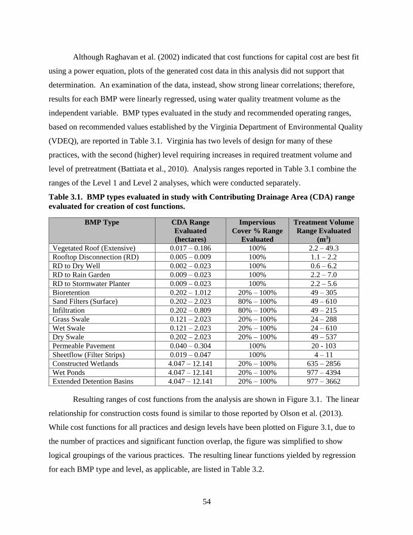
54
Although Raghavan et al. (2002) indicated that cost functions for capital cost are best fit
using a power equation, plots of the generated cost data in this analysis did not support that
determination. An examination of the data, instead, show strong linear correlations; therefore,
results for each BMP were linearly regressed, using water quality treatment volume as the
independent variable. BMP types evaluated in the study and recommended operating ranges,
based on recommended values established by the Virginia Department of Environmental Quality
(VDEQ), are reported in Table 3.1. Virginia has two levels of design for many of these
practices, with the second (higher) level requiring increases in required treatment volume and
level of pretreatment (Battiata et al., 2010). Analysis ranges reported in Table 3.1 combine the
ranges of the Level 1 and Level 2 analyses, which were conducted separately.
Table 3.1. BMP types evaluated in study with Contributing Drainage Area (CDA) range
evaluated for creation of cost functions.
BMP Type CDA Range
Evaluated
(hectares)
Impervious
Cover % Range
Evaluated
Treatment Volume
Range Evaluated
(m3)
Vegetated Roof (Extensive) 0.017 – 0.186 100% 2.2 – 49.3
Rooftop Disconnection (RD) 0.005 – 0.009 100% 1.1 – 2.2
RD to Dry Well 0.002 – 0.023 100% 0.6 – 6.2
RD to Rain Garden 0.009 – 0.023 100% 2.2 – 7.0
RD to Stormwater Planter 0.009 – 0.023 100% 2.2 – 5.6
Bioretention 0.202 – 1.012 20% – 100% 49 – 305
Sand Filters (Surface) 0.202 – 2.023 80% – 100% 49 – 610
Infiltration 0.202 – 0.809 80% – 100% 49 – 215
Grass Swale 0.121 – 2.023 20% – 100% 24 – 288
Wet Swale 0.121 – 2.023 20% – 100% 24 – 610
Dry Swale 0.202 – 2.023 20% – 100% 49 – 537
Permeable Pavement 0.040 – 0.304 100% 20 - 103
Sheetflow (Filter Strips) 0.019 – 0.047 100% 4 – 11
Constructed Wetlands 4.047 – 12.141 20% – 100% 635 – 2856
Wet Ponds 4.047 – 12.141 20% – 100% 977 – 4394
Extended Detention Basins 4.047 – 12.141 20% – 100% 977 – 3662
Resulting ranges of cost functions from the analysis are shown in Figure 3.1. The linear
relationship for construction costs found is similar to those reported by Olson et al. (2013).
While cost functions for all practices and design levels have been plotted on Figure 3.1, due to
the number of practices and significant function overlap, the figure was simplified to show
logical groupings of the various practices. The resulting linear functions yielded by regression
for each BMP type and level, as applicable, are listed in Table 3.2.
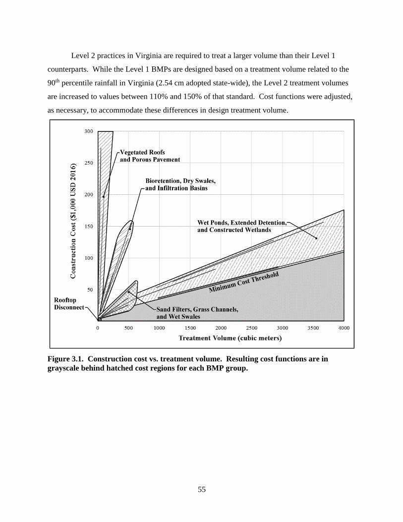
55
Level 2 practices in Virginia are required to treat a larger volume than their Level 1
counterparts. While the Level 1 BMPs are designed based on a treatment volume related to the
90th percentile rainfall in Virginia (2.54 cm adopted state-wide), the Level 2 treatment volumes
are increased to values between 110% and 150% of that standard. Cost functions were adjusted,
as necessary, to accommodate these differences in design treatment volume.
Figure 3.1. Construction cost vs. treatment volume. Resulting cost functions are in
grayscale behind hatched cost regions for each BMP group.
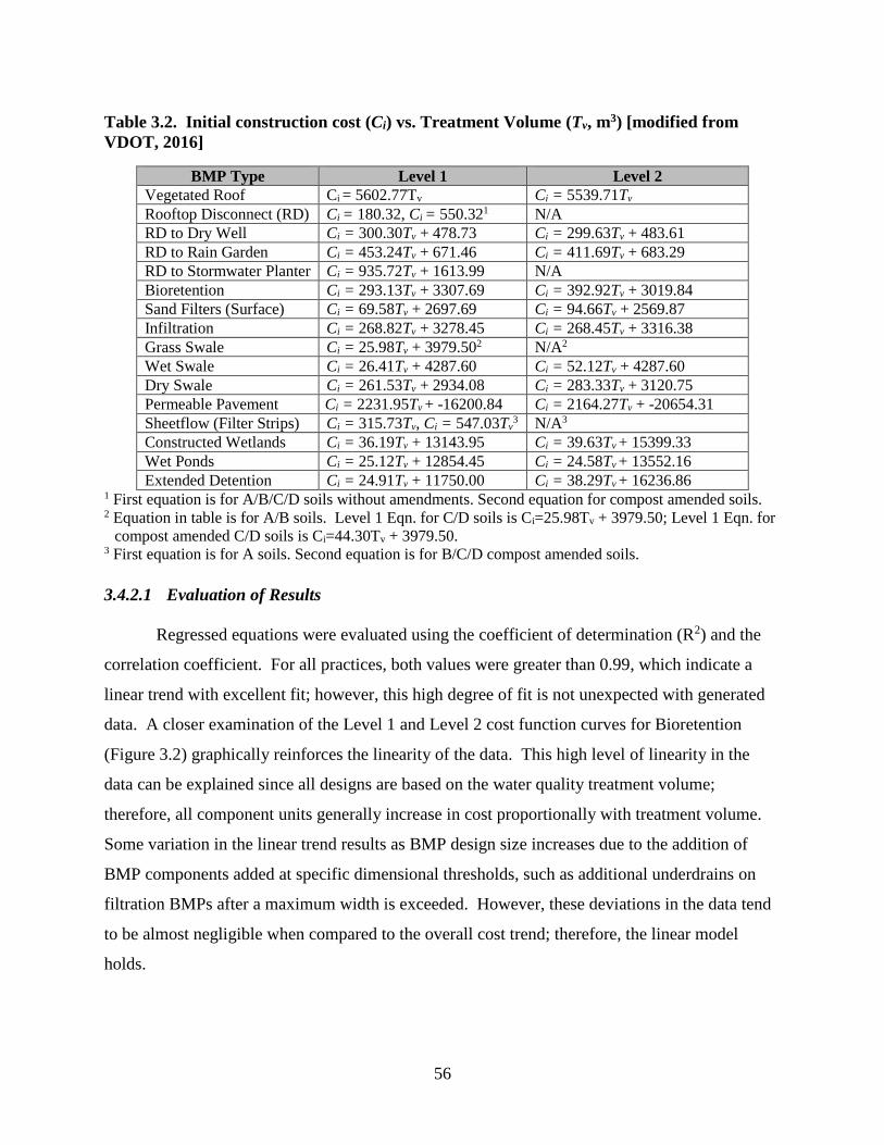
56
Table 3.2. Initial construction cost (Ci) vs. Treatment Volume (Tv, m3) [modified from
VDOT, 2016]
BMP Type Level 1 Level 2
Vegetated Roof Ci = 5602.77Tv Ci = 5539.71Tv
Rooftop Disconnect (RD) Ci = 180.32, Ci = 550.321 N/A
RD to Dry Well Ci = 300.30Tv + 478.73 Ci = 299.63Tv + 483.61
RD to Rain Garden Ci = 453.24Tv + 671.46 Ci = 411.69Tv + 683.29
RD to Stormwater Planter Ci = 935.72Tv + 1613.99 N/A
Bioretention Ci = 293.13Tv + 3307.69 Ci = 392.92Tv + 3019.84
Sand Filters (Surface) Ci = 69.58Tv + 2697.69 Ci = 94.66Tv + 2569.87
Infiltration Ci = 268.82Tv + 3278.45 Ci = 268.45Tv + 3316.38
Grass Swale Ci = 25.98Tv + 3979.502 N/A2
Wet Swale Ci = 26.41Tv + 4287.60 Ci = 52.12Tv + 4287.60
Dry Swale Ci = 261.53Tv + 2934.08 Ci = 283.33Tv + 3120.75
Permeable Pavement Ci = 2231.95Tv + -16200.84 Ci = 2164.27Tv + -20654.31
Sheetflow (Filter Strips) Ci = 315.73Tv, Ci = 547.03Tv3 N/A3
Constructed Wetlands Ci = 36.19Tv + 13143.95 Ci = 39.63Tv + 15399.33
Wet Ponds Ci = 25.12Tv + 12854.45 Ci = 24.58Tv + 13552.16
Extended Detention Ci = 24.91Tv + 11750.00 Ci = 38.29Tv + 16236.86 1 First equation is for A/B/C/D soils without amendments. Second equation for compost amended soils. 2 Equation in table is for A/B soils. Level 1 Eqn. for C/D soils is Ci=25.98Tv + 3979.50; Level 1 Eqn. for
compost amended C/D soils is Ci=44.30Tv + 3979.50. 3 First equation is for A soils. Second equation is for B/C/D compost amended soils.
3.4.2.1 Evaluation of Results
Regressed equations were evaluated using the coefficient of determination (R2) and the
correlation coefficient. For all practices, both values were greater than 0.99, which indicate a
linear trend with excellent fit; however, this high degree of fit is not unexpected with generated
data. A closer examination of the Level 1 and Level 2 cost function curves for Bioretention
(Figure 3.2) graphically reinforces the linearity of the data. This high level of linearity in the
data can be explained since all designs are based on the water quality treatment volume;
therefore, all component units generally increase in cost proportionally with treatment volume.
Some variation in the linear trend results as BMP design size increases due to the addition of
BMP components added at specific dimensional thresholds, such as additional underdrains on
filtration BMPs after a maximum width is exceeded. However, these deviations in the data tend
to be almost negligible when compared to the overall cost trend; therefore, the linear model
holds.
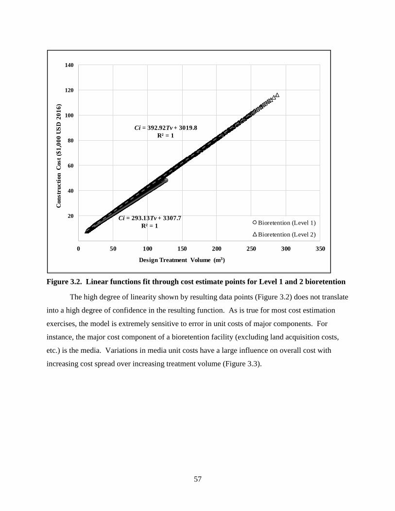
57
Figure 3.2. Linear functions fit through cost estimate points for Level 1 and 2 bioretention
The high degree of linearity shown by resulting data points (Figure 3.2) does not translate
into a high degree of confidence in the resulting function. As is true for most cost estimation
exercises, the model is extremely sensitive to error in unit costs of major components. For
instance, the major cost component of a bioretention facility (excluding land acquisition costs,
etc.) is the media. Variations in media unit costs have a large influence on overall cost with
increasing cost spread over increasing treatment volume (Figure 3.3).
Ci = 293.13Tv + 3307.7
R² = 1
Ci = 392.92Tv + 3019.8
R² = 1
20
40
60
80
100
120
140
0 50 100 150 200 250 300 350
Con
str
ucti
on
C
ost
($1
,00
0 U
SD
20
16
)
Design Treatment Volume (m3)
Bioretention (Level 1)
Bioretention (Level 2)
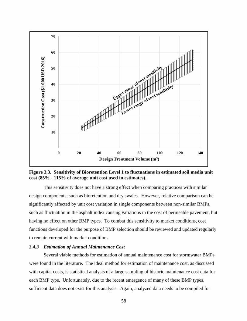
58
Figure 3.3. Sensitivity of Bioretention Level 1 to fluctuations in estimated soil media unit
cost (85% - 115% of average unit cost used in estimates).
This sensitivity does not have a strong effect when comparing practices with similar
design components, such as bioretention and dry swales. However, relative comparison can be
significantly affected by unit cost variation in single components between non-similar BMPs,
such as fluctuation in the asphalt index causing variations in the cost of permeable pavement, but
having no effect on other BMP types. To combat this sensitivity to market conditions, cost
functions developed for the purpose of BMP selection should be reviewed and updated regularly
to remain current with market conditions.
3.4.3 Estimation of Annual Maintenance Cost
Several viable methods for estimation of annual maintenance cost for stormwater BMPs
were found in the literature. The ideal method for estimation of maintenance cost, as discussed
with capital costs, is statistical analysis of a large sampling of historic maintenance cost data for
each BMP type. Unfortunately, due to the recent emergence of many of these BMP types,
sufficient data does not exist for this analysis. Again, analyzed data needs to be compiled for
10
20
30
40
50
60
70
0 20 40 60 80 100 120 140
Co
nstr
ucti
on
Co
st (
$1
,000 U
SD
20
16)
Design Treatment Volume (m3)
59
similarly designed practices, which often means that database consolidation at a national level
has limited merit due to regional variation between BMP design standards. To combat this
limitation, two other methods have been suggested in the literature.
The first is a more time intensive method that includes estimating tasks, materials, and
labor for ‘normal’ years and ‘extensive upkeep’ years, and averaging those costs. Conceptually,
this method is similar to that explained above for generation of opinions of expected costs.
Taylor et al. (2014) uses this method in the development of spreadsheets for estimating the whole
life cycle cost of various highway related stormwater BMP retrofits. WERF (2005) also
integrates this methodology in its analysis of O&M costs. WERF reported that factors, such as
proximity of closest disposal site, rather than labor, materials, and tasks at the BMP location
often have a larger effect on overall maintenance cost.
A second, more commonly used method found in the literature, is estimation of O&M
costs as a percentage of construction cost (USEPA, 1999; Weiss et al., 2007; MPCA, 2011; King
and Hagan, 2011). King and Hagan (2011) describe a general trend among O&M costs related to
construction cost where the O&M percentage cost for stormwater BMPs decreases with
increasing initial installation cost. Weiss et al. (2007) performed an updated analysis of O&M
costs for comparison to USEPA (1999). That data, in addition to values derived from component
costs computed from an analysis by King and Hagan (2011) and evaluation of BMPs using
Taylor et al. (2014) spreadsheets over those ranges found in Table 3.1, are shown in Table 3.3.
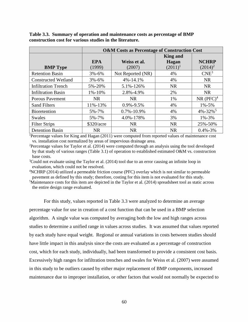
60
Table 3.3. Summary of operation and maintenance costs as percentage of BMP
construction cost for various studies in the literature.
O&M Costs as Percentage of Construction Cost
BMP Type
EPA
(1999) Weiss et al.
(2007)
King and
Hagan
(2011)1 NCHRP
(2014)2
Retention Basin 3%-6% Not Reported (NR) 4% CNE3
Constructed Wetland 3%-6% 4%-14.1% 4% NR
Infiltration Trench 5%-20% 5.1%-126% NR NR
Infiltration Basin 1%-10% 2.8%-4.9% 2% NR
Porous Pavement NR NR 1% NR (PFC)4
Sand Filters 11%-13% 0.9%-9.5% 4% 1%-5%
Bioretention 5%-7% 0.7%-10.9% 4% 4%-32%5
Swales 5%-7% 4.0%-178% 3% 1%-3%
Filter Strips $320/acre NR NR 25%-50%
Detention Basin NR NR NR 0.4%-3% 1Percentage values for King and Hagan (2011) were computed from reported values of maintenance cost
vs. installation cost normalized by areas of impervious drainage area. 2Percentage values for Taylor et al. (2014) were computed through an analysis using the tool developed
by that study of various ranges (Table 3.1) of operation to established estimated O&M vs. construction
base costs. 3Could not evaluate using the Taylor et al. (2014) tool due to an error causing an infinite loop in
evaluation, which could not be resolved. 4NCHRP (2014) utilized a permeable friction course (PFC) overlay which is not similar to permeable
pavement as defined by this study; therefore, costing for this item is not evaluated for this study. 5Maintenance costs for this item are depicted in the Taylor et al. (2014) spreadsheet tool as static across
the entire design range evaluated.
For this study, values reported in Table 3.3 were analyzed to determine an average
percentage value for use in creation of a cost function that can be used in a BMP selection
algorithm. A single value was computed by averaging both the low and high ranges across
studies to determine a unified range in values across studies. It was assumed that values reported
by each study have equal weight. Regional or annual variations in costs between studies should
have little impact in this analysis since the costs are evaluated as a percentage of construction
cost, which for each study, individually, had been transformed to provide a consistent cost basis.
Excessively high ranges for infiltration trenches and swales for Weiss et al. (2007) were assumed
in this study to be outliers caused by either major replacement of BMP components, increased
maintenance due to improper installation, or other factors that would not normally be expected to
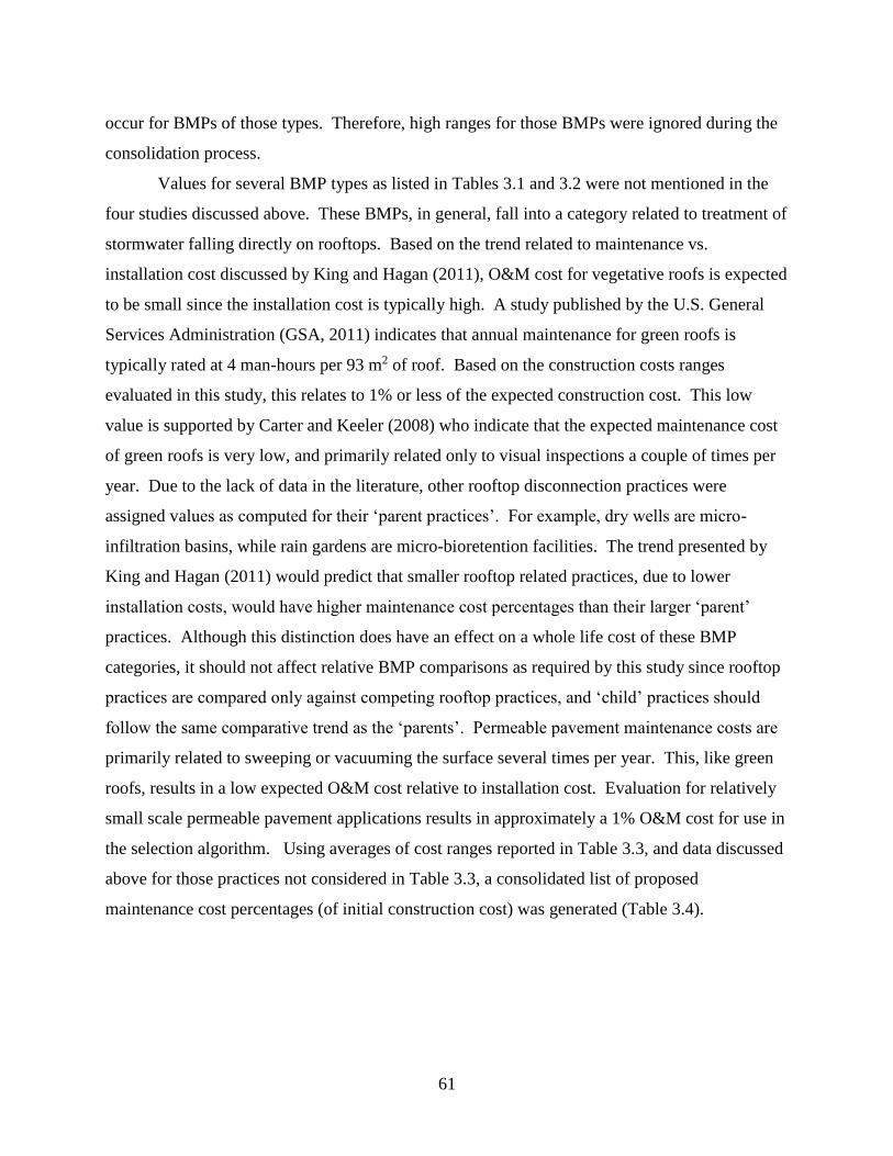
61
occur for BMPs of those types. Therefore, high ranges for those BMPs were ignored during the
consolidation process.
Values for several BMP types as listed in Tables 3.1 and 3.2 were not mentioned in the
four studies discussed above. These BMPs, in general, fall into a category related to treatment of
stormwater falling directly on rooftops. Based on the trend related to maintenance vs.
installation cost discussed by King and Hagan (2011), O&M cost for vegetative roofs is expected
to be small since the installation cost is typically high. A study published by the U.S. General
Services Administration (GSA, 2011) indicates that annual maintenance for green roofs is
typically rated at 4 man-hours per 93 m2 of roof. Based on the construction costs ranges
evaluated in this study, this relates to 1% or less of the expected construction cost. This low
value is supported by Carter and Keeler (2008) who indicate that the expected maintenance cost
of green roofs is very low, and primarily related only to visual inspections a couple of times per
year. Due to the lack of data in the literature, other rooftop disconnection practices were
assigned values as computed for their ‘parent practices’. For example, dry wells are micro-
infiltration basins, while rain gardens are micro-bioretention facilities. The trend presented by
King and Hagan (2011) would predict that smaller rooftop related practices, due to lower
installation costs, would have higher maintenance cost percentages than their larger ‘parent’
practices. Although this distinction does have an effect on a whole life cost of these BMP
categories, it should not affect relative BMP comparisons as required by this study since rooftop
practices are compared only against competing rooftop practices, and ‘child’ practices should
follow the same comparative trend as the ‘parents’. Permeable pavement maintenance costs are
primarily related to sweeping or vacuuming the surface several times per year. This, like green
roofs, results in a low expected O&M cost relative to installation cost. Evaluation for relatively
small scale permeable pavement applications results in approximately a 1% O&M cost for use in
the selection algorithm. Using averages of cost ranges reported in Table 3.3, and data discussed
above for those practices not considered in Table 3.3, a consolidated list of proposed
maintenance cost percentages (of initial construction cost) was generated (Table 3.4).
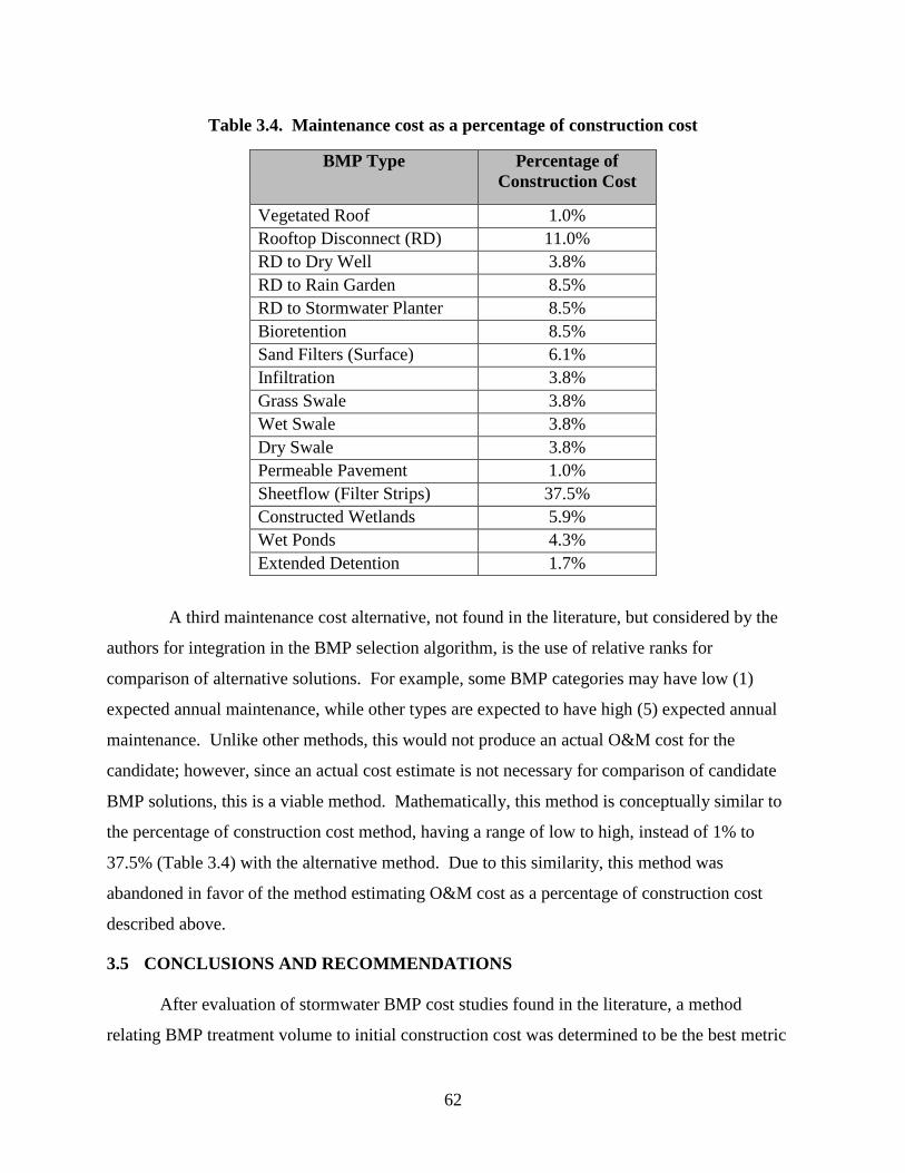
62
Table 3.4. Maintenance cost as a percentage of construction cost
BMP Type Percentage of
Construction Cost
Vegetated Roof 1.0%
Rooftop Disconnect (RD) 11.0%
RD to Dry Well 3.8%
RD to Rain Garden 8.5%
RD to Stormwater Planter 8.5%
Bioretention 8.5%
Sand Filters (Surface) 6.1%
Infiltration 3.8%
Grass Swale 3.8%
Wet Swale 3.8%
Dry Swale 3.8%
Permeable Pavement 1.0%
Sheetflow (Filter Strips) 37.5%
Constructed Wetlands 5.9%
Wet Ponds 4.3%
Extended Detention 1.7%
A third maintenance cost alternative, not found in the literature, but considered by the
authors for integration in the BMP selection algorithm, is the use of relative ranks for
comparison of alternative solutions. For example, some BMP categories may have low (1)
expected annual maintenance, while other types are expected to have high (5) expected annual
maintenance. Unlike other methods, this would not produce an actual O&M cost for the
candidate; however, since an actual cost estimate is not necessary for comparison of candidate
BMP solutions, this is a viable method. Mathematically, this method is conceptually similar to
the percentage of construction cost method, having a range of low to high, instead of 1% to
37.5% (Table 3.4) with the alternative method. Due to this similarity, this method was
abandoned in favor of the method estimating O&M cost as a percentage of construction cost
described above.
3.5 CONCLUSIONS AND RECOMMENDATIONS
After evaluation of stormwater BMP cost studies found in the literature, a method
relating BMP treatment volume to initial construction cost was determined to be the best metric
63
for use in an algorithm aimed at optimization of BMP selection in treatment trains. Treatment
volume, as defined in this article, includes the WQV as computed with Equation 1 and any
additional contributions arising as effluent from upstream BMPs. The methods outlined in this
paper for construction of cost estimates using a unit cost data approach were applied to BMP
types used in the Commonwealth of Virginia. Cost functions relating construction cost to
treatment volume that resulted from these data points were shown to have a high linear
correlation. Despite this high correlation of resulting functions, a sensitivity analysis was
performed to verify the expected high degree of sensitivity of the cost function data to
fluctuations in unit costs of BMP components. Use in a comparison algorithm limits the
sensitivity to unit cost variation since absolute cost is not as important as relative cost between
candidate solutions.
A review of O&M cost studies revealed several methods for computation of annual
maintenance cost for stormwater BMPs. Of these methods, the method that reports O&M cost as
a percentage of construction cost is the most prevalent. Summaries of maintenance cost ranges
from various studies were collected and analyzed to determine an average percent maintenance
cost for this study. Papers detailing these percent ranges contained little or no commentary
regarding data used to establish the published ranges, therefore, the efficacy of the data is
unknown. Several suspected outliers were omitted when computing average cost percentages for
final values reported in this study.
Resulting functions listed in Table 3.2 are applicable to BMPs designed and installed in
the Commonwealth of Virginia; however, the unit cost method for determining these functions
can be applied universally. Further, if used for cost estimation, functions listed in Table 3.2 were
specifically determined for the southwest Virginia region and should be adjusted for regional
variation if used in other areas of the state. However, when using for comparison and selection
between BMPs, which is the focus of this study, adjustment should not be necessary, since
comparative and not absolute cost is the determining factor. Percent values of O&M costs
(Table 3.4) should be applicable nationally, since data originally used to create ranges found in
various studies was adjusted to provide a consistent cost basis.
64
3.6 REFERENCES
Battiata, J., Collins, K., Hirschman, D., and Hoffmann, G. (2010). “The Runoff Reduction
Method.”, Journal of Contemporary Water Research & Education, 146, 11-21.
Brown, W. and Schueler, T. (1997). The Economics of Storm Water BMPs in the Mid-Atlantic
Region. Center for Watershed Protection. Ellicott City, MD.
California Department of Transportation (Caltrans) (2004). BMP retrofit pilot program—
Appendix C3. Final Report, Division of Environmental Analysis, Caltrans, Sacramento,
California.
Carter, T. and Keeler, A. (2008). “Life-cycle cost-benefit analysis of extensive vegetated roof
systems.” Journal of Environmental Management, 87(2008), pp. 350-363.
Center for Watershed Protection (CWP) (2013). “Cost-Effectiveness Study of Urban Stormwater
BMPs in the James River Basin.” Ellicott City, MD.
<http://www.jamesriverassociation.org/what-we-do/JRA-Cost-effective-Full-Report-
June-update.pdf> (March 21, 2016).
Cheng, M., Zhen, J., and Shoemaker, L. (2009). “BMP Decision Support System for Evaluating
Stormwater Management Alternatives”, Frontiers of Environmental Science and
Engineering. 3(4): 453-463.
International Stormwater BMP Database (ISBMPD) (2014). “International BMP Database.”
Version 12 30 2014, <http://www.bmpdatabase.org> (January 15, 2016).
King, D. and Hagan, P. (2011). “Costs of Stormwater Management Practices in Maryland
Counties.” University of Maryland Center for Environmental Science. CBL 11-043.
Landphair, H.C., McFalls, J.A., and Thompson, D. (2000). Design methods, selections, and
cost-effectiveness of stormwater quality structures. Texas Transportation Institute, Texas
A&M University System, College Station, Texas.
Livingston, E., Shaver, E., Skupien, J., and Horner, R. (1997). Operation, Maintenance and
Management of Storm Water Management Systems. Watershed Management Institute.
Ingleside, MD.
Long, Daniel L. and Randel L. Dymond (2013). “Thermal Pollution Mitigation in Cold Water
Stream Watersheds Using Bioretention.” Journal of the American Water Resources
Association (JAWRA) 50(4): 977-987. DOI: 10.1111/jawr.12152
Maryland Department of the Environment (MDE) (2009). “2000 Maryland Stormwater Design
Manual”. Water Management Administration and Center for Watershed Protection, rev.
2009.
<http://www.mde.state.md.us/programs/water/stormwatermanagementprogram/maryland
stormwaterdesignmanual/Pages/Programs/WaterPrograms/SedimentandStormwater/stor
mwater_design/index.aspx> (September 25, 2015).

65
Moran, A., and Hunt, B. (2004). BMP cost estimate study. North Carolina State University,
Raleigh, N.C.
Minnesota Pollution Control Agency (MPCA) (2011). “Best Management Practices
Construction Costs, Maintenance Costs, and Land Requirement.”
<https://www.pca.state.mn.us/sites/default/files/p-gen3-13x.pdf> (April 10, 2016).
New York Department of Environmental Conservation (2015). “New York State Stormwater
Management Design Manual.” <http://www.dec.ny.gov/chemical/29072.html> (April
18, 2016).
North Carolina Department of Environmental and Natural Resources (NCDENR) (2007).
“Stormwater BMP Manual.” <http://portal.ncdenr.org/web/lr/bmp-manual> (September
25, 2015)
Olson, C., Roesner, L., Urbonas, B., MacKenzie, K. (2013). BMP REALCOST Best
Management Practices – Rational Estimation of Actual Likely Costs of Stormwater
Treatment, A Spreadsheet Tool for Evaluating BMP Effectiveness and Life Cycle Costs,
User’s Manual and Documentation. Version 1.21.
Raghavan, R., Koustas, R., and Liao, S. (2002). “Cost Estimating for Best Management
Practices.” Proc., Linking Stormwater BMP Designs and Performance to Receiving
Water Impact Mitigation, ASCE, Reston, Va., 539-543. doi: 10.1061/40602(263)42
Shoemaker, L., Riverson, J., Alvi, K., Zhen, J., Paul, S., Rafi, T. (2009). “SUSTAIN—A
Framework for Placement of Best Management Practices in Urban Watersheds to Protect
Water Quality”. Cincinnati, OH: USEPA (U. S. Environmental Protection Agency)
National Risk Management Research Laboratory. EPA/600/R09/095.
Schueler, T. (1987). Controlling urban runoff: a practical manual for planning and designing
urban BMPs. Metropolitan Washington Council of Governments. Washington, DC.
Schueler, T. (1997). “Comparative Removal Capability of Urban BMPs: A Reanalysis.”
Watershed Protection Techniques. 1(2), 515-520.
Schueler, T. and Youngk, A. (2015). “Potential Benefits of Nutrient and Sediment Practices to
Reduce Toxic Contaminants in the Chesapeake Bay Watershed.” Chesapeake
Stormwater Network.
<http://www.chesapeakebay.net/documents/Final_Report_on_Urban_Toxic_Contaminan
ts.pdf.> (April 21, 2016).
Southeastern Wisconsin Regional Planning Commission (SWRPC) (1991). Costs of Urban
Nonpoint Source Water Pollution Control Measures. Waukesha, WI.
Taylor, S., Barrett, M., Leisenring, M., Sahu, S., Pankani, D., Poresky, A., Questad, A., Strecker,
E., Weinstein, N., and Venner, M. (2014). “Long-Term Performance and Life-Cycle
Costs of Stormwater Best Management Practices.” Transportation Research Board of the
National Academies, Washington, DC.
66
United States Environmental Protection Agency (USEPA) (1999). Preliminary data summary of
urban stormwater best management practices. EPA-821-R-99-012, Washington, D.C.
United States Environmental Protection Agency (USEPA) (2005). “Stormwater Phase II Final
Rule.” Office of Water Fact Sheet. Publication No. EPA 833-F-00-002.
United States Environmental Protection Agency (USEPA) (2011). Enhanced Framework
(SUSTAIN) and Field Applications for Placement of BMPs in Urban Watersheds.
Publication No. EPA/600/R-11/144.
United States Environmental Protection Agency (USEPA) (2016). “NPDES Stormwater Permit
Program.”< https://www3.epa.gov/region1/npdes/stormwater/ > (April 4, 2016).
United States Environmental Protection Agency (USEPA) (2014). “SUSTAIN Version 1.2”. <
https://www.epa.gov/water-research/system-urban-stormwater-treatment-and-analysis-
integration-sustain> (January 28, 2016).
United States General Services Agency (GSA) (2011). “The Benefits and Challenges of Green
Roofs on Public and Commercial Buildings.”
<http://www.gsa.gov/portal/mediaId/158783/fileName/The_Benefits_and_Challenges_of
_Green_Roofs_on_Public_and_Commercial_Buildings.action> (April 23, 2016)
Virginia Department of Environmental Quality (VDEQ) (2013a). Stormwater Management
Handbook, version 2.0, Draft. Commonwealth of Virginia, Richmond, Virginia.
Virginia Department of Conservation and Recreation (VDCR) (2013b). Virginia DCR
Stormwater Design Specification No. 9 Bioretention, Draft. Commonwealth of Virginia,
Richmond, Virginia.
Virginia Department of Transportation (VDOT) (2016). “VDOT Stormwater BMP Selection
Optimization Tool User Guide”. Virginia Center for Transportation Innovation and
Research. Charlottesville, VA.
Water Environment Research Foundation (WERF) (2005). Performance and Whole Life Costs
of Best Management Practices and Sustainable Urban Drainage Systems. Report # 01-
CTS-21T.
Water Environment Research Foundation (WERF) (2013). “BMP Select Model Version 2.0 and
User’s Guide”. Project #SWC1R06c. <
https://www.werf.org/a/ka/Search/ResearchProfile.aspx?ReportId=SWC1R06c >
(February 23, 2016).
Weiss, P., Gulliver, J., and Erickson, A. (2007). "Cost and Pollutant Removal of Storm-Water
Treatment Practices." J. Water Resources Planning Management, 133:3(218), 218-229.
West Virginia Department of Environmental Protection (2012). “West Virginia Stormwater
Management and Design Guidance Manual”.

67
<http://www.dep.wv.gov/WWE/Programs/stormwater/MS4/Pages/StormwaterManageme
ntDesignandGuidanceManual.aspx> (September 25, 2015).
Wiegand, C., Schueler, T., Shittenden, W., and Jellick, D. (1986). “Cost of Urban Runoff
Controls.” Proc., Urban Runoff Quality Impact and Quality Enhancement Technology.
Engineering Foundation Conference, Henniker, NH.
Young, K., Dymond, R., and Kibler, D. (2011). "Development of an Improved Approach for
Selecting Storm-Water Best Management Practices." J. Water Resour. Plann. Manage.,
10.1061/(ASCE)WR.1943-5452.0000110, 268-275.
68
Chapter 4: Case Study: Integration of Optimization Software into the
Engineering Design Process for Stormwater BMP Selection
Hodges, C.C.1, Dymond, R.L.2, Young, K.D.3
Status: This manuscript will be submitted for peer review and publication after completion of
the dissertation defense.
4.1 ABSTRACT
Low impact development (LID) strategies are being increasingly employed to provide for
a holistic treatment of stormwater runoff from developed sites. Designers are required to
simultaneously consider pollutant load reductions, physical site constraints, and selection
criteria, including cost when making selections. Due to the large number of constraints,
selection priorities, and best management practice (BMP) configurations, designers frequently
resort to choosing known solutions strategies that are excessive is reduction of pollutant loads
and costlier than an optimal configuration. This manuscript describes development of a software
model for optimal selection of stormwater treatment BMPs. A release version of the software is
developed incorporating the Virginia Runoff Reduction Method (VRRM) in development of the
objective function. Two case studies are developed and applied to a group of consulting
engineers to determine the effect that use of the selection optimization tool has on the
engineering design process. Results of the case study indicate that use of a selection
optimization algorithm for stormwater BMP selection significantly alters the engineering design
process by removing bias and allowing designers to spend more time evaluating solutions rather
than attempting to meet regulatory objectives.
1 Graduate Research Assistant, Via Department of Civil and Environmental Engineering,
Virginia Tech, 200 Patton Hall, Blacksburg, VA 24061 (e-mail: [email protected]) 2 Associate Professor, Via Department of Civil and Environmental Engineering, Virginia Tech,
200 Patton Hall, Blacksburg, VA 24061 (e-mail: [email protected]) 3 Professor of Practice, Via Department of Civil and Environmental Engineering, Virginia Tech,
200 Patton Hall, Blacksburg, VA 24061 (e-mail: [email protected])
69
4.2 INTRODUCTION
Increasing urbanization, and the resulting increase in impervious cover has led to a
degradation in the quality of the Nation’s waters (Dietz and Clausen, 2008). Impacts to surface
waters include increased volume, pollutant loads, temperature, and potential decreases to base
flow (Elliott and Trowsdale, 2007). Prior to enactment of the Clean Water Act (CWA, 1972)
stormwater management focused primarily on flood and erosion control. Recently, with
adoption of the CWA and its amendments, a paradigm shift has spurred state level regulations
that address additional stormwater runoff components, including volume and quality. This
development has resulted in less reliance on impounding/detention facilities and more on low
impact development (LID) strategies distributed throughout a development site. LID strategies
are employed with the goal of mimicking pre-development hydrologic response in post-
development sites (USEPA, 2000). Techniques employed by such practices can include both
non-structural strategies, such as disturbance minimization, and structural practices such as
bioretention, permeable pavement, grass swales, etc. (Dietz, 2007; Battiata et al., 2010).
Integration of these LID best management practices (BMPs) may have a higher implementation
cost than regional basins; however, they can be more cost effective on a long term pollutant
reduction and volume retention and abatement basis (Dietz, 2007; Montalto et al., 2007).
Despite cost concerns, in order to meet pollutant reduction mandates for discharges to surface
waters, most states have now published stormwater BMP manuals (NCDENR, 2007; MDE,
2009; West Virginia (WVDEP), 2012; VDEQ, 2013b; and others) that provide BMP types and
specifications which promote the use of LID strategies similar to practices described by the
United States Environmental Protection Agency (USEPA, 2000).
There has been increasing recognition that runoff volume reduction is necessary to
effectively reach pollutant reduction goals (Battiata et al., 2010). Battiata describes a compliance
strategy called the Runoff Reduction Method (RRM) (Hirschman et al., 2008) which uses a
three-tiered approach for treatment that sequentially addresses reduction goals through 1)
minimization measures, 2) runoff reduction measures, and, if necessary, 3) pollutant reduction
measures. Since it is uncommon for development projects to reach goals solely through
minimization strategies, engineers increasingly are tasked with providing designs and
computations employing runoff and pollutant reduction strategies. Attempting to provide the
necessary tools to aid design engineers in the compliance of both runoff and pollutant reduction
70
through BMPs, the Center for Watershed Protection (CWP), in cooperation with the Virginia
Department of Conservation and Recreation (VDCR) developed a Virginia RRM (VRRM)
spreadsheet tool (VDEQ, 2016a) based on the RRM methods first introduced by Hirschman et al.
(2008). Battiata et al. (2010) describe the RRM method as transferable to a wide array of state
and local stormwater planning operations, with the Commonwealth of Virginia being one of the
first states to employ this method.
Although LID strategies are becoming more common, engineers today are often using
design tools that are not specifically tailored for tracking runoff reduction (Dietz, 2007) and
nutrient removal. The need for new, more intelligent tools to aid engineers has become more
pressing due to distributed BMP designs, often linked to form a sequence of BMPs in series
called a ‘treatment train’ (Wong et al., 2006). Tracking pollutant and volume reductions through
treatment train components requires the ability to evaluate partially treated effluent entering a
downstream BMP from upstream BMP(s), in addition to untreated surface influent. This need
was addressed in Virginia through distribution of the VRRM spreadsheets (VDEQ, 2016a),
which were established to provide a tool that aids designers with application of the VRRM.
Though early tools have provided the ability to track pollutant and runoff reduction
through treatment trains, they do not identify the optimal BMP configuration. Most tools, such
as the VRRM spreadsheets, have simple interfaces that allow single configuration input and
testing, but are not targeted at yielding the optimized solution. Engineers, increasingly, need a
unified stormwater BMP selection tool that simultaneously considers siting constraints with user
specified selection criteria, while allowing rapid iteration through all valid BMP configurations.
The goal of this study is to create and implement a stormwater BMP selection tool that meets this
need. To quantify the effect that this tool has on the engineering design process, two BMP
selection case studies were presented to a group of stormwater design professionals in Virginia to
provide a comparison of solutions using the selection optimization tool versus the VRRM
spreadsheets (VDEQ, 2016a), as the control.
4.3 VRRM SPREADSHEET TOOL
The VRRM (VDEQ, 2016a) spreadsheets provide designers with a tool that allows
computation of required nutrient (phosphorus) reductions, and methods for inputting and
tracking pollutant loads and runoff reduction for single BMP or treatment train configurations.
71
Required phosphorus load reductions are computed for new or re-development projects based on
user input of pre-development and post-development land cover and drainage area data, as
applicable. ‘Drainage area tabs’ allow input and tracking of runoff reduction and phosphorus
removal based on total mass removal according to methods outlined in Hirschman et al. (2008).
Finally, the tool provides adjusted curve numbers, which Hirschman et al. (2008) describe as a
means to approximate the hydrologic impact of the BMP to downstream runoff. While the tool
is effective in providing support for design engineers for single BMP installations, applicability
for designs employing treatment trains becomes more cumbersome since it is not intended to
provide engineers with the ability to rapidly consider multiple BMP combinations.
The VRRM method and spreadsheets are limited in nature, and were designed as a
compliance tool for computing and meeting required nutrient reductions on development sites.
The method does not enable a full hydrologic analysis of the site for complying with required
quantity control in the developed state. It also provides no direction related to the design of the
selected BMPs, including required pretreatment measures, which must be performed by
engineers using other guidance documents.
4.4 CANDIDATE BMPS USED IN VRRM
Battiata et al. (2010) describes BMP runoff reduction and pollutant removal practices that
can be employed as part of the RRM. Battiata et al. further describes ranges of runoff reduction
and pollutant removal values for each BMP, with the lower value in the range representing the
median runoff/pollutant removal values based on a CWP literature review. These lower range
values are assigned the designation ‘Level 1’ treatment devices by Battiata et al. (2010).
Likewise, the upper value in the range is assigned the designation of ‘Level 2’ treatment device
based on the 75th percentile value resulting from the statistical analysis of studies from the
literature as analyzed by Battiata et al. (2010). Accounting for BMP treatment strategies that
employ a Level 1 and Level 2 designation, as applicable, and those that have a single ‘level’,
there are 37 unique non-proprietary BMP types that are currently employed as part of the VRRM
computational methodology (Table 4.1).
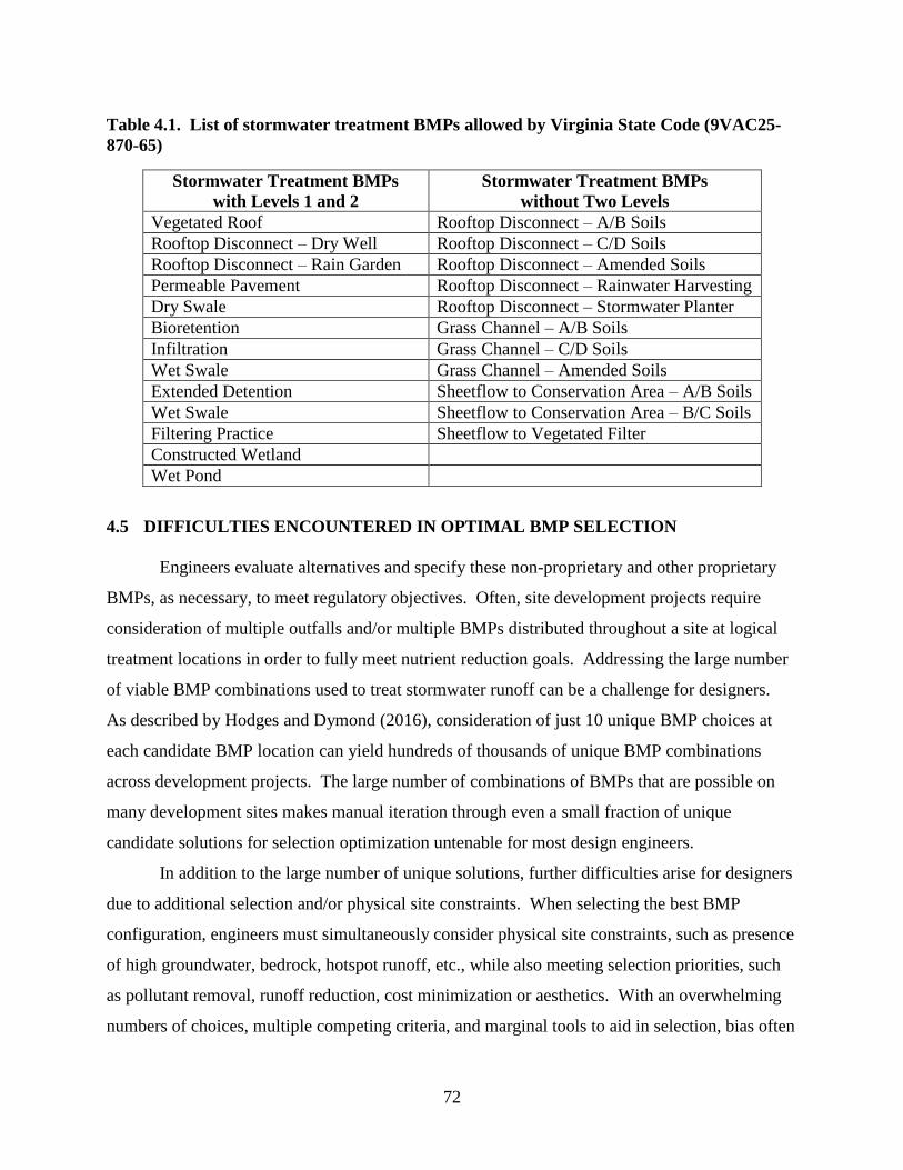
72
Table 4.1. List of stormwater treatment BMPs allowed by Virginia State Code (9VAC25-
870-65)
Stormwater Treatment BMPs
with Levels 1 and 2
Stormwater Treatment BMPs
without Two Levels
Vegetated Roof Rooftop Disconnect – A/B Soils
Rooftop Disconnect – Dry Well Rooftop Disconnect – C/D Soils
Rooftop Disconnect – Rain Garden Rooftop Disconnect – Amended Soils
Permeable Pavement Rooftop Disconnect – Rainwater Harvesting
Dry Swale Rooftop Disconnect – Stormwater Planter
Bioretention Grass Channel – A/B Soils
Infiltration Grass Channel – C/D Soils
Wet Swale Grass Channel – Amended Soils
Extended Detention Sheetflow to Conservation Area – A/B Soils
Wet Swale Sheetflow to Conservation Area – B/C Soils
Filtering Practice Sheetflow to Vegetated Filter
Constructed Wetland
Wet Pond
4.5 DIFFICULTIES ENCOUNTERED IN OPTIMAL BMP SELECTION
Engineers evaluate alternatives and specify these non-proprietary and other proprietary
BMPs, as necessary, to meet regulatory objectives. Often, site development projects require
consideration of multiple outfalls and/or multiple BMPs distributed throughout a site at logical
treatment locations in order to fully meet nutrient reduction goals. Addressing the large number
of viable BMP combinations used to treat stormwater runoff can be a challenge for designers.
As described by Hodges and Dymond (2016), consideration of just 10 unique BMP choices at
each candidate BMP location can yield hundreds of thousands of unique BMP combinations
across development projects. The large number of combinations of BMPs that are possible on
many development sites makes manual iteration through even a small fraction of unique
candidate solutions for selection optimization untenable for most design engineers.
In addition to the large number of unique solutions, further difficulties arise for designers
due to additional selection and/or physical site constraints. When selecting the best BMP
configuration, engineers must simultaneously consider physical site constraints, such as presence
of high groundwater, bedrock, hotspot runoff, etc., while also meeting selection priorities, such
as pollutant removal, runoff reduction, cost minimization or aesthetics. With an overwhelming
numbers of choices, multiple competing criteria, and marginal tools to aid in selection, bias often
73
creeps into the selection process. Jacob et al. (2007) describe how memory of past decisions can
cause designers to choose solutions similar to past designs regardless of applicability current
needs. Tools such as the VRRM spreadsheets (VDEQ, 2016a) only partially address the
difficulty associated with compliance computations for design of distributed BMP networks.
Although they do afford designers the ability to track volume and nutrient reduction through
BMP networks for candidate solutions, they do not allow for rapid iteration through potentially
thousands of viable solutions. The end result is that for complicated sites, to save time, designers
often steer to non-optimized conservative solutions which meet regulatory load reduction
objectives, but often provide excess pollutant removal at higher cost than the optimal solution.
In order to eliminate this selection bias, a multiple criteria optimization algorithm is required to
facilitate BMP selection in distributed stormwater networks based on objective evaluation of user
ranked parameters, consideration of site constraints, and simultaneous analysis of required
pollutant reduction goals.
4.6 MODEL DEVELOPMENT AND DESIGN
The optimization model was designed to operate as a standalone software tool with
relatively low data input requirements and processor overhead. This more streamlined design
was implemented in part to address an apparent disconnect between many software tools that are
developed to fill a niche need and require extensive datasets and user input for operation.
Typically, these systems are so data intensive that they cannot be considered for everyday use by
most engineering consultants. This software’s interface is presented to the user as a simple
tabbed interface, which allows rapid guided navigation by the user when developing solutions for
computing and meeting required phosphorus load reduction goals.
Treatment train input is similar to that found in many other hydrologic software products
(USACE, 2015) and generally implements the node and link graphical model, which allows the
user to add and link BMPs in a treatment train configuration, as required (Figure 4.1).
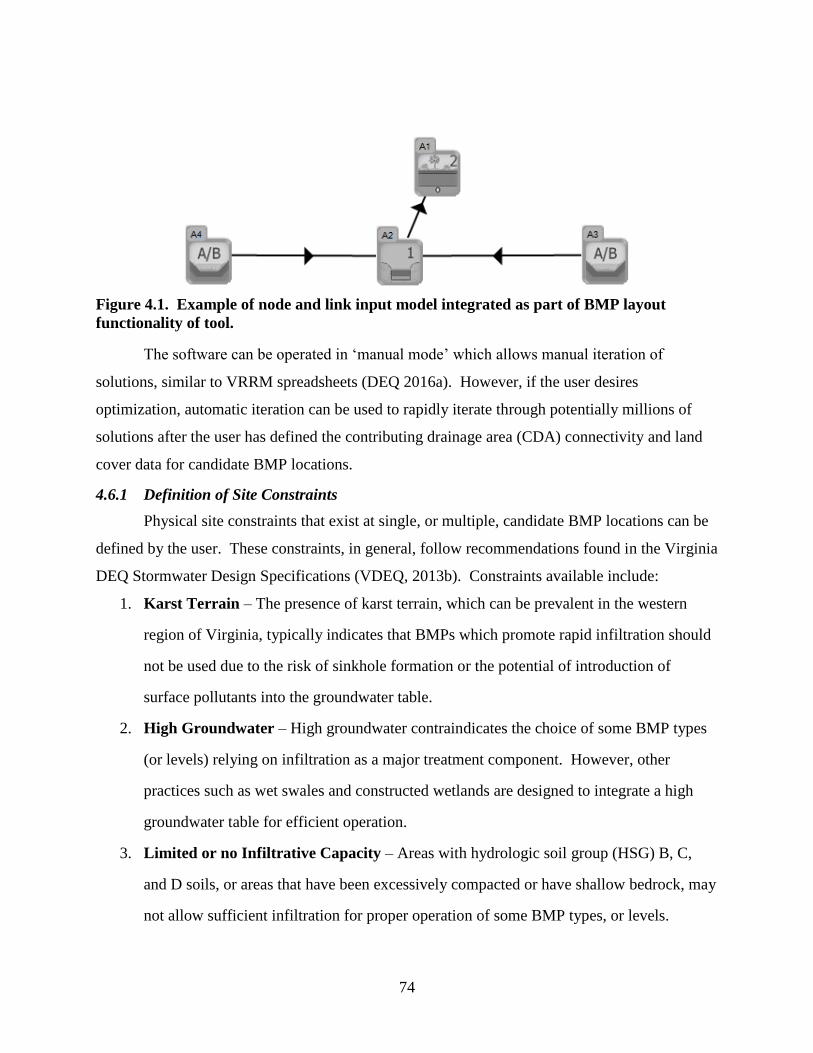
74
Figure 4.1. Example of node and link input model integrated as part of BMP layout
functionality of tool.
The software can be operated in ‘manual mode’ which allows manual iteration of
solutions, similar to VRRM spreadsheets (DEQ 2016a). However, if the user desires
optimization, automatic iteration can be used to rapidly iterate through potentially millions of
solutions after the user has defined the contributing drainage area (CDA) connectivity and land
cover data for candidate BMP locations.
4.6.1 Definition of Site Constraints
Physical site constraints that exist at single, or multiple, candidate BMP locations can be
defined by the user. These constraints, in general, follow recommendations found in the Virginia
DEQ Stormwater Design Specifications (VDEQ, 2013b). Constraints available include:
1. Karst Terrain – The presence of karst terrain, which can be prevalent in the western
region of Virginia, typically indicates that BMPs which promote rapid infiltration should
not be used due to the risk of sinkhole formation or the potential of introduction of
surface pollutants into the groundwater table.
2. High Groundwater – High groundwater contraindicates the choice of some BMP types
(or levels) relying on infiltration as a major treatment component. However, other
practices such as wet swales and constructed wetlands are designed to integrate a high
groundwater table for efficient operation.
3. Limited or no Infiltrative Capacity – Areas with hydrologic soil group (HSG) B, C,
and D soils, or areas that have been excessively compacted or have shallow bedrock, may
not allow sufficient infiltration for proper operation of some BMP types, or levels.
75
4. CDA Subject to Hotspot Runoff – Hotspot areas are those that exhibit higher than
normal concentrations of surface pollutants. Areas that are subject to hotspot runoff,
typically have parking or high traffic areas as part of the CDA which indicates the
presence of hydrocarbons or toxic metals in surface runoff. BMPs that promote rapid
infiltration or integrate a high water table are contraindicated in these areas.
5. Coastal Plain – Several BMPs are not recommended for use in the coastal plain area due
to the presence of high groundwater. Modifications to other BMPs, such as wet ponds,
are required when they are designed and implemented in these areas.
4.6.2 Elimination of BMPs Prior to Optimization
To reduce computational time during the optimization process, BMPs that cannot be used
due to physical site constraints, or other connectivity issues should be eliminated. These
strategies are not unique to this tool, and in fact form the basis of several other publications or
software tools that aid in the selection of BMPs. Maryland (MDE, 2009) provides matrices to
aid in BMP selection, but provides little guidance in computation of load reductions through
treatment trains. Selection tools addressing BMP selection include the Colorado Urban Drainage
and Flood Control District UD-BMP (UDFCD, 2010), Ohio DOT BMP selection tool (ORIL,
2015), the White River Alliance (WRA) BMP Selection Tool (WRA, 2016), BMPSELECT
(Pomeroy and Rowney, 2013) and several others. Most of these tools are simple web-based or
spreadsheet based tools that allow the user to indicate if various site features and/or constraints
are present on the project site. From this user input, many BMPs are eliminated from
consideration, leaving the user with a candidate list of BMPs that may be suitable for the project.
At this point, it is the designer’s responsibility to use ‘best judgement’ in selecting the
appropriate BMP for the site from the remaining list. Although these programs are useful in
eliminating candidates that do not meet project constraints, the programs do not rank the list of
candidate BMPs based on additional user input and cannot deal with large numbers of candidate
BMP combinations expected in treatment train configurations; therefore, the danger of bias in
selecting BMPs when using these tools still remains.
Depending on the number of outfalls and BMPs, elimination of a single BMP choice
could eliminate hundreds to thousands of candidate combinations. Hodges and Dymond (2016)
discuss several weeding techniques that have been implemented in the development of the
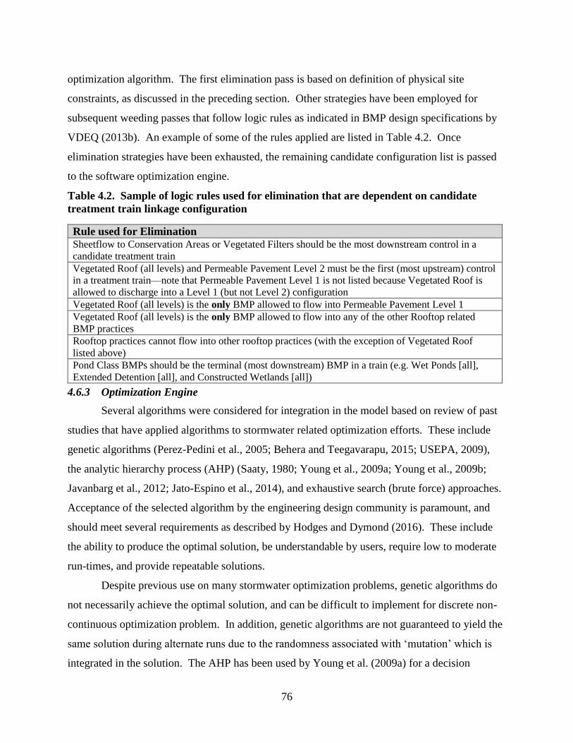
76
optimization algorithm. The first elimination pass is based on definition of physical site
constraints, as discussed in the preceding section. Other strategies have been employed for
subsequent weeding passes that follow logic rules as indicated in BMP design specifications by
VDEQ (2013b). An example of some of the rules applied are listed in Table 4.2. Once
elimination strategies have been exhausted, the remaining candidate configuration list is passed
to the software optimization engine.
Table 4.2. Sample of logic rules used for elimination that are dependent on candidate
treatment train linkage configuration
Rule used for Elimination Sheetflow to Conservation Areas or Vegetated Filters should be the most downstream control in a
candidate treatment train
Vegetated Roof (all levels) and Permeable Pavement Level 2 must be the first (most upstream) control
in a treatment train—note that Permeable Pavement Level 1 is not listed because Vegetated Roof is
allowed to discharge into a Level 1 (but not Level 2) configuration
Vegetated Roof (all levels) is the only BMP allowed to flow into Permeable Pavement Level 1
Vegetated Roof (all levels) is the only BMP allowed to flow into any of the other Rooftop related
BMP practices
Rooftop practices cannot flow into other rooftop practices (with the exception of Vegetated Roof
listed above)
Pond Class BMPs should be the terminal (most downstream) BMP in a train (e.g. Wet Ponds [all],
Extended Detention [all], and Constructed Wetlands [all])
4.6.3 Optimization Engine
Several algorithms were considered for integration in the model based on review of past
studies that have applied algorithms to stormwater related optimization efforts. These include
genetic algorithms (Perez-Pedini et al., 2005; Behera and Teegavarapu, 2015; USEPA, 2009),
the analytic hierarchy process (AHP) (Saaty, 1980; Young et al., 2009a; Young et al., 2009b;
Javanbarg et al., 2012; Jato-Espino et al., 2014), and exhaustive search (brute force) approaches.
Acceptance of the selected algorithm by the engineering design community is paramount, and
should meet several requirements as described by Hodges and Dymond (2016). These include
the ability to produce the optimal solution, be understandable by users, require low to moderate
run-times, and provide repeatable solutions.
Despite previous use on many stormwater optimization problems, genetic algorithms do
not necessarily achieve the optimal solution, and can be difficult to implement for discrete non-
continuous optimization problem. In addition, genetic algorithms are not guaranteed to yield the
same solution during alternate runs due to the randomness associated with ‘mutation’ which is
integrated in the solution. The AHP has been used by Young et al. (2009a) for a decision
77
support tool related to BMP selection; however, the AHP requires the generation of static
matrices for evaluation which would be dependent on each trial configuration of BMP solutions.
This requirement adds an additional step to the computational procedure beyond what is required
by the exhaustive search method, which would only act to reduce optimization speed.
Exhaustive search (ES) can be easily understood since at its essence, all possible solutions are
attempted through iteration, with the optimal candidate being selected from the final solution set.
After evaluating the ability of each of the algorithms to meet the four criteria listed above,
Hodges and Dymond (2016) concluded that an exhaustive search algorithm was the best choice
for meeting selection objectives.
Optimization is defined as the maximization or minimization of a model’s objective
function. The objective function for this study is based on maximization of a solution score
which has five major components. These selection criteria include minimization of excess
nutrient removal, minimization of installation cost, minimization of maintenance cost,
maximization of runoff reduction, and maximization of aesthetic benefit (if any). The nutrient
removal and runoff reduction functions used in model development is based on the VRRM;
although, development of an objective function derived from other standards can be developed
and applied. Full descriptions of the nutrient removal, runoff reduction, and aesthetics functions
are found in Hodges and Dymond (2016), while a complete discussion of the installation and
maintenance cost functions are found in Hodges et al. (2016). Solutions are optimized based on
user weights applied to each of the selection criteria listed above, in addition to physical site
constraints and CDA descriptive parameters.
Prioritization is based on a zero (0) to ten (10) scale, with a value of zero giving no
weight to the associated parameter, while a value of ten, conversely, yields the highest weight.
Prior to optimization, the user can modify these values, as desired, including setting parameter
weights to equivalent values. Final solution scores and configuration ranking are directly
dependent on this user weighting.
4.7 CASE STUDIES
The release version of the selection optimization tool was applied to two case studies at a
site scale to determine its impact on BMP selection by design engineers. A group of land
development/water resources engineers with at least one year of design experience were
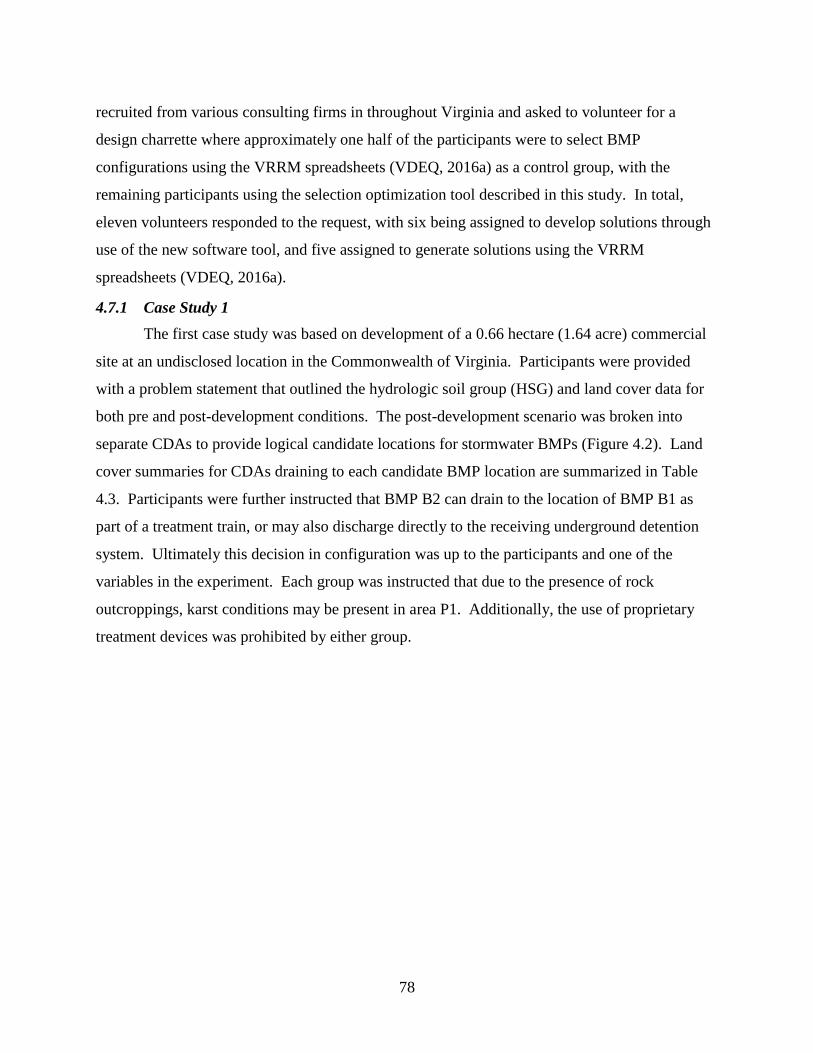
78
recruited from various consulting firms in throughout Virginia and asked to volunteer for a
design charrette where approximately one half of the participants were to select BMP
configurations using the VRRM spreadsheets (VDEQ, 2016a) as a control group, with the
remaining participants using the selection optimization tool described in this study. In total,
eleven volunteers responded to the request, with six being assigned to develop solutions through
use of the new software tool, and five assigned to generate solutions using the VRRM
spreadsheets (VDEQ, 2016a).
4.7.1 Case Study 1
The first case study was based on development of a 0.66 hectare (1.64 acre) commercial
site at an undisclosed location in the Commonwealth of Virginia. Participants were provided
with a problem statement that outlined the hydrologic soil group (HSG) and land cover data for
both pre and post-development conditions. The post-development scenario was broken into
separate CDAs to provide logical candidate locations for stormwater BMPs (Figure 4.2). Land
cover summaries for CDAs draining to each candidate BMP location are summarized in Table
4.3. Participants were further instructed that BMP B2 can drain to the location of BMP B1 as
part of a treatment train, or may also discharge directly to the receiving underground detention
system. Ultimately this decision in configuration was up to the participants and one of the
variables in the experiment. Each group was instructed that due to the presence of rock
outcroppings, karst conditions may be present in area P1. Additionally, the use of proprietary
treatment devices was prohibited by either group.
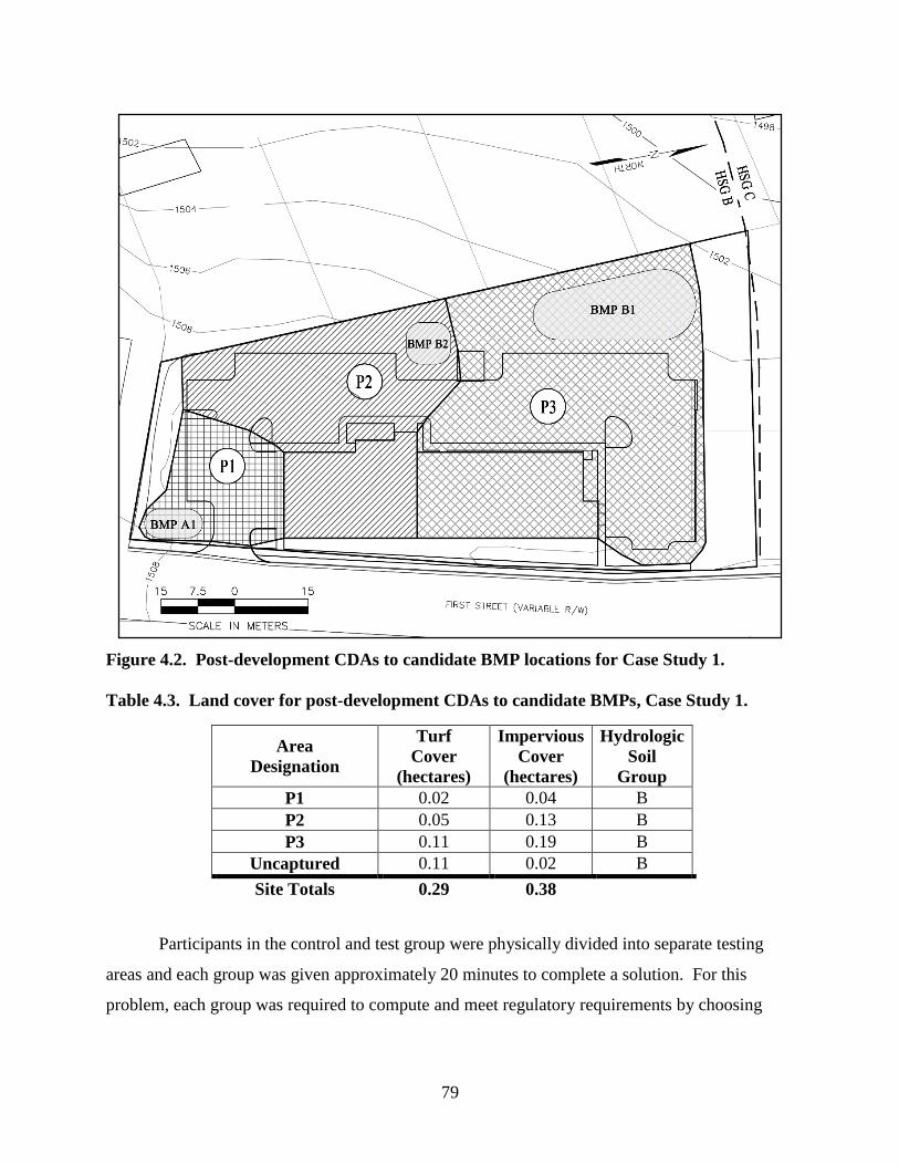
79
Figure 4.2. Post-development CDAs to candidate BMP locations for Case Study 1.
Table 4.3. Land cover for post-development CDAs to candidate BMPs, Case Study 1.
Area
Designation
Turf
Cover
(hectares)
Impervious
Cover
(hectares)
Hydrologic
Soil
Group
P1 0.02 0.04 B
P2 0.05 0.13 B
P3 0.11 0.19 B
Uncaptured 0.11 0.02 B
Site Totals 0.29 0.38
Participants in the control and test group were physically divided into separate testing
areas and each group was given approximately 20 minutes to complete a solution. For this
problem, each group was required to compute and meet regulatory requirements by choosing
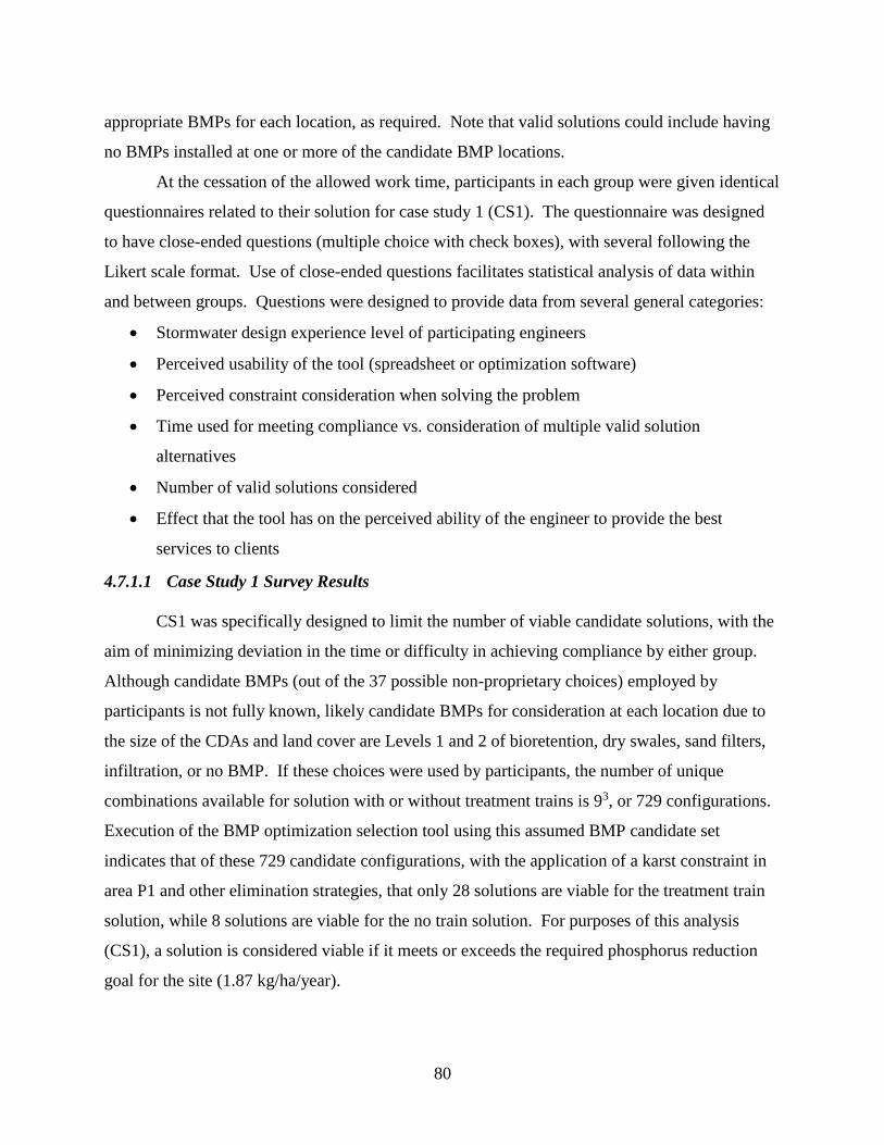
80
appropriate BMPs for each location, as required. Note that valid solutions could include having
no BMPs installed at one or more of the candidate BMP locations.
At the cessation of the allowed work time, participants in each group were given identical
questionnaires related to their solution for case study 1 (CS1). The questionnaire was designed
to have close-ended questions (multiple choice with check boxes), with several following the
Likert scale format. Use of close-ended questions facilitates statistical analysis of data within
and between groups. Questions were designed to provide data from several general categories:
Stormwater design experience level of participating engineers
Perceived usability of the tool (spreadsheet or optimization software)
Perceived constraint consideration when solving the problem
Time used for meeting compliance vs. consideration of multiple valid solution
alternatives
Number of valid solutions considered
Effect that the tool has on the perceived ability of the engineer to provide the best
services to clients
4.7.1.1 Case Study 1 Survey Results
CS1 was specifically designed to limit the number of viable candidate solutions, with the
aim of minimizing deviation in the time or difficulty in achieving compliance by either group.
Although candidate BMPs (out of the 37 possible non-proprietary choices) employed by
participants is not fully known, likely candidate BMPs for consideration at each location due to
the size of the CDAs and land cover are Levels 1 and 2 of bioretention, dry swales, sand filters,
infiltration, or no BMP. If these choices were used by participants, the number of unique
combinations available for solution with or without treatment trains is 93, or 729 configurations.
Execution of the BMP optimization selection tool using this assumed BMP candidate set
indicates that of these 729 candidate configurations, with the application of a karst constraint in
area P1 and other elimination strategies, that only 28 solutions are viable for the treatment train
solution, while 8 solutions are viable for the no train solution. For purposes of this analysis
(CS1), a solution is considered viable if it meets or exceeds the required phosphorus reduction
goal for the site (1.87 kg/ha/year).
81
4.7.1.1.1 Case Study 1 Qualitative Results
All participants obtained solutions that achieved compliance goals; however, there were
prominent differences between the two groups with regards to how the allotted time was used in
achieving solutions. Generally, the spreadsheet group initially implemented BMPs with known
high phosphorus reduction capabilities and then tested other viable candidates with lower
phosphorus removal efficiencies to obtain, first, a valid solution, and then a more site specific
solution, as time allowed. The software optimization group, instead, entered all viable CDA land
cover data and viewed the optimized solutions, spending more time on testing the treatment
train/no treatment train scenarios, or adjusting optimization ranks to determine differences in
optimization solutions when runoff reduction, nutrient removal, or cost parameters were given
higher weight. Although the software optimization group had never used the software
previously, the participants appeared to embrace the optimized results offered by the tool.
4.7.1.1.2 Case Study 1 Quantitative Results
Frequency analysis was performed on collected data from post solution questionnaires to
determine the percentage of respondents that fell within each response category. Median values
were also determined for each individual question to provide indication of central tendency.
Based on responses, all participants had greater than 2 years of experience in stormwater site
design, with the median value of both groups, as assessed both separately and combined, falling
in the ‘5 – 10 year’ range. Overall, the combined groups indicated that they had used the VRRM
spreadsheets (DEQ, 2016a) on ‘10 – 20’ projects; however, the software group had a median that
fell within the ‘5 – 10’ project range, while the control had slightly more experience, falling in
the ‘10 – 20’ project bin.
Participants were asked to assess the assigned tool’s usability related to several general
categories, including:
Data entry
Treatment train connectivity and visualization
Consideration of site constraints
Rapid iteration through additional treatment scenarios
Tool’s ability to reduce repetitive design tasks
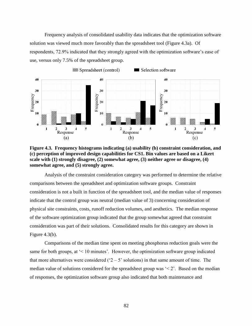
82
Frequency analysis of consolidated usability data indicates that the optimization software
solution was viewed much more favorably than the spreadsheet tool (Figure 4.3a). Of
respondents, 72.9% indicated that they strongly agreed with the optimization software’s ease of
use, versus only 7.5% of the spreadsheet group.
Figure 4.3. Frequency histograms indicating (a) usability (b) constraint consideration, and
(c) perception of improved design capabilities for CS1. Bin values are based on a Likert
scale with (1) strongly disagree, (2) somewhat agree, (3) neither agree or disagree, (4)
somewhat agree, and (5) strongly agree.
Analysis of the constraint consideration category was performed to determine the relative
comparisons between the spreadsheet and optimization software groups. Constraint
consideration is not a built in function of the spreadsheet tool, and the median value of responses
indicate that the control group was neutral (median value of 3) concerning consideration of
physical site constraints, costs, runoff reduction volumes, and aesthetics. The median response
of the software optimization group indicated that the group somewhat agreed that constraint
consideration was part of their solutions. Consolidated results for this category are shown in
Figure 4.3(b).
Comparisons of the median time spent on meeting phosphorus reduction goals were the
same for both groups, at ‘< 10 minutes’. However, the optimization software group indicated
that more alternatives were considered (‘2 – 5’ solutions) in that same amount of time. The
median value of solutions considered for the spreadsheet group was ‘< 2’. Based on the median
of responses, the optimization software group also indicated that both maintenance and
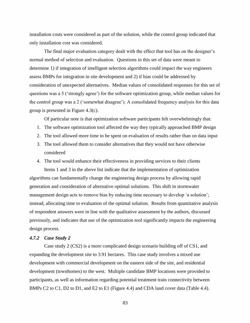
83
installation costs were considered as part of the solution, while the control group indicated that
only installation cost was considered.
The final major evaluation category dealt with the effect that tool has on the designer’s
normal method of selection and evaluation. Questions in this set of data were meant to
determine 1) if integration of intelligent selection algorithms could impact the way engineers
assess BMPs for integration in site development and 2) if bias could be addressed by
consideration of unexpected alternatives. Median values of consolidated responses for this set of
questions was a 5 (‘strongly agree’) for the software optimization group, while median values for
the control group was a 2 (‘somewhat disagree’). A consolidated frequency analysis for this data
group is presented in Figure 4.3(c).
Of particular note is that optimization software participants felt overwhelmingly that:
1. The software optimization tool affected the way they typically approached BMP design
2. The tool allowed more time to be spent on evaluation of results rather than on data input
3. The tool allowed them to consider alternatives that they would not have otherwise
considered
4. The tool would enhance their effectiveness in providing services to their clients
Items 1 and 3 in the above list indicate that the implementation of optimization
algorithms can fundamentally change the engineering design process by allowing rapid
generation and consideration of alternative optimal solutions. This shift in stormwater
management design acts to remove bias by reducing time necessary to develop ‘a solution’;
instead, allocating time to evaluation of the optimal solution. Results from quantitative analysis
of respondent answers were in line with the qualitative assessment by the authors, discussed
previously, and indicates that use of the optimization tool significantly impacts the engineering
design process.
4.7.2 Case Study 2
Case study 2 (CS2) is a more complicated design scenario building off of CS1, and
expanding the development site to 3.91 hectares. This case study involves a mixed use
development with commercial development on the eastern side of the site, and residential
development (townhomes) to the west. Multiple candidate BMP locations were provided to
participants, as well as information regarding potential treatment train connectivity between
BMPs C2 to C1, D2 to D1, and E2 to E1 (Figure 4.4) and CDA land cover data (Table 4.4).
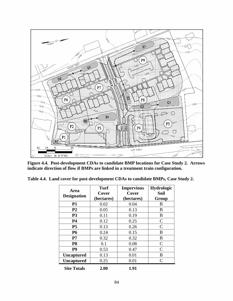
84
Figure 4.4. Post-development CDAs to candidate BMP locations for Case Study 2. Arrows
indicate direction of flow if BMPs are linked in a treatment train configuration.
Table 4.4. Land cover for post-development CDAs to candidate BMPs, Case Study 2.
Area
Designation
Turf
Cover
(hectares)
Impervious
Cover
(hectares)
Hydrologic
Soil
Group
P1 0.02 0.04 B
P2 0.05 0.13 B
P3 0.11 0.19 B
P4 0.12 0.25 C
P5 0.13 0.26 C
P6 0.24 0.15 B
P7 0.32 0.32 B
P8 0.1 0.08 C
P9 0.53 0.47 C
Uncaptured 0.13 0.01 B
Uncaptured 0.25 0.01 C
Site Totals 2.00 1.91
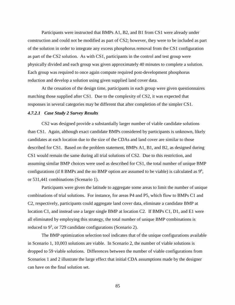
85
Participants were instructed that BMPs A1, B2, and B1 from CS1 were already under
construction and could not be modified as part of CS2; however, they were to be included as part
of the solution in order to integrate any excess phosphorus removal from the CS1 configuration
as part of the CS2 solution. As with CS1, participants in the control and test group were
physically divided and each group was given approximately 40 minutes to complete a solution.
Each group was required to once again compute required post-development phosphorus
reduction and develop a solution using given supplied land cover data.
At the cessation of the design time, participants in each group were given questionnaires
matching those supplied after CS1. Due to the complexity of CS2, it was expected that
responses in several categories may be different that after completion of the simpler CS1.
4.7.2.1 Case Study 2 Survey Results
CS2 was designed provide a substantially larger number of viable candidate solutions
than CS1. Again, although exact candidate BMPs considered by participants is unknown, likely
candidates at each location due to the size of the CDAs and land cover are similar to those
described for CS1. Based on the problem statement, BMPs A1, B1, and B2, as designed during
CS1 would remain the same during all trial solutions of CS2. Due to this restriction, and
assuming similar BMP choices were used as described for CS1, the total number of unique BMP
configurations (if 8 BMPs and the no BMP option are assumed to be viable) is calculated as 96,
or 531,441 combinations (Scenario 1).
Participants were given the latitude to aggregate some areas to limit the number of unique
combinations of trial solutions. For instance, for areas P4 and P5, which flow to BMPs C1 and
C2, respectively, participants could aggregate land cover data, eliminate a candidate BMP at
location C1, and instead use a larger single BMP at location C2. If BMPs C1, D1, and E1 were
all eliminated by employing this strategy, the total number of unique BMP combinations is
reduced to 93, or 729 candidate configurations (Scenario 2).
The BMP optimization selection tool indicates that of the unique configurations available
in Scenario 1, 10,003 solutions are viable. In Scenario 2, the number of viable solutions is
dropped to 59 viable solutions. Differences between the number of viable configurations from
Scenarios 1 and 2 illustrate the large effect that initial CDA assumptions made by the designer
can have on the final solution set.
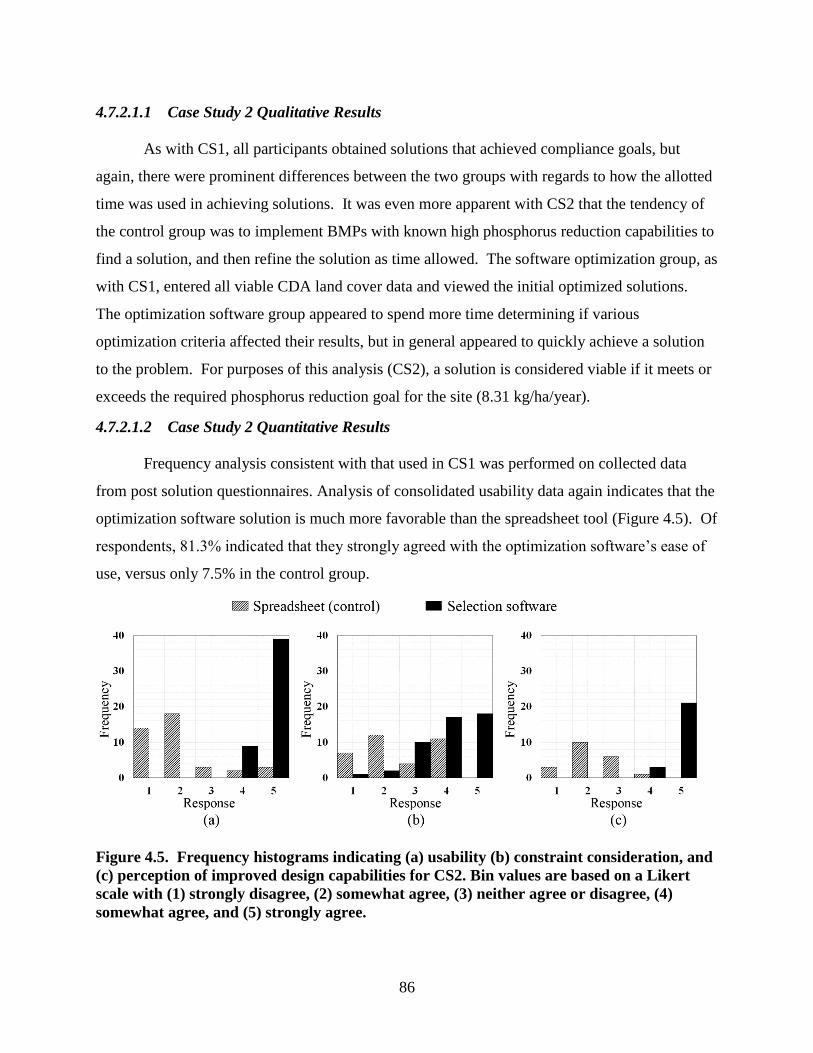
86
4.7.2.1.1 Case Study 2 Qualitative Results
As with CS1, all participants obtained solutions that achieved compliance goals, but
again, there were prominent differences between the two groups with regards to how the allotted
time was used in achieving solutions. It was even more apparent with CS2 that the tendency of
the control group was to implement BMPs with known high phosphorus reduction capabilities to
find a solution, and then refine the solution as time allowed. The software optimization group, as
with CS1, entered all viable CDA land cover data and viewed the initial optimized solutions.
The optimization software group appeared to spend more time determining if various
optimization criteria affected their results, but in general appeared to quickly achieve a solution
to the problem. For purposes of this analysis (CS2), a solution is considered viable if it meets or
exceeds the required phosphorus reduction goal for the site (8.31 kg/ha/year).
4.7.2.1.2 Case Study 2 Quantitative Results
Frequency analysis consistent with that used in CS1 was performed on collected data
from post solution questionnaires. Analysis of consolidated usability data again indicates that the
optimization software solution is much more favorable than the spreadsheet tool (Figure 4.5). Of
respondents, 81.3% indicated that they strongly agreed with the optimization software’s ease of
use, versus only 7.5% in the control group.
Figure 4.5. Frequency histograms indicating (a) usability (b) constraint consideration, and
(c) perception of improved design capabilities for CS2. Bin values are based on a Likert
scale with (1) strongly disagree, (2) somewhat agree, (3) neither agree or disagree, (4)
somewhat agree, and (5) strongly agree.
87
There were minor differences in the results from the questions concerning constraint
consideration in solutions between CS1 and CS2 [Figures 4.2(b) and 4.4(b)]. Although several
control participants strongly agreed that various constraints were considered during CS1, none
strongly agreed that any of the constraints were considered during CS2. This result may be due
to the time required for control participants to obtain a valid nutrient removal solution. It is
suspected from observation of the group that so much time was spent on achieving a valid
solution, that little time was available for consideration of site constraints. Results for the
software group were similar between CS2 and CS1; although, there were some marginal
improvements in the ‘strongly agree’ category for the CS2 solution.
Comparisons of the median time spent on meeting phosphorus reduction goals was ‘10 -
20 minutes’ for the control group, and “< 10 minutes” for the software group. Both groups
indicated that a similar number of alternatives were considered. However, due to the ambiguity
of the question, it is unknown if respondents believed this to mean full solutions, or
modifications to BMP types at individual locations. The perceived ability of the tool used by
each group to modify/improve the design process for engineers was similar to CS1. Median
values of consolidated responses for this set of questions was, again, a 5 (‘strongly agree’) for the
software optimization group, while median values for the control group was a 2 (‘somewhat
disagree’) [Figure 4.2(c)].
4.7.3 General Results
In general, quantitative results from CS1 and CS2 are similar. This implies that
complexity of design problem does not have a significant impact on comparison of the software
tool to the control group. Based on this result, it is inferred that improvements to the engineering
design process imparted through use of the software tool is scalable to designs of varying
magnitude. Overwhelmingly, respondents utilizing the software optimization tool believed that
use of the tool allowed consideration of alternatives that would not have otherwise been
considered, enhanced their efficiency in design, and most strikingly, affected the way that they
typically approach BMP design. Based on these case study results, it appears that the tool was
successful in reducing bias in stormwater BMP selection. Although the sample size of
volunteers for this study was not large enough to constitute a full representative sample for
extension to the full population of design engineers in the Commonwealth of Virginia, it is
88
believed that based on the consistency of responses that results are translatable to the larger
population.
4.8 CONCLUSIONS
Based on the prevalence of distributed LID techniques in stormwater designs, it is
imperative that tools are developed to assist designers in selecting the optimal BMP
configuration that takes into account constraints and selection criteria in an unbiased manner.
The goal of this study was to test an optimization algorithm that was developed by the authors
through implementation of a proof of concept model based on the VRRM nutrient and runoff
reduction tracking procedures that was evaluated by practicing engineers. Based on results of
CS1 and CS2, it is apparent that development of such tools can boost efficiency and help to
minimize bias from the BMP selection process. Although the model was well received by the
participants, as related to the evaluation of CS1 and CS2, there is future work that needs to be
performed to improve the functioning or expand the scope of the model.
For large sites with multiple outfalls and treatment train configurations, long run times
may be required to achieve an optimal solution. As discussed in Hodges and Dymond (2016),
based on Virginia Stormwater Management Permit (VSMP) data (VDEQ, 2016b), most projects
requiring water quality improvements are expected to have a relatively small number of outfalls
and treatment train components. However, for those that fall outside the range, run times can be
excessive, which complicates use by designers. One solution to combat excessive run times is
application of an intra-outfall optimization where a percentage of the overall load removal for the
site is distributed across outfalls based on the weighted percentage of generated post-
development load in each. Although this method would significantly decrease run times for
generation of results, it is unlikely to produce the optimal configuration of BMPs across outfalls.
This trade off, however, may be acceptable to designers due to time constraints and the large
number of combinatorial solutions.
This study has applied the VRRM with the regulatory runoff reduction and phosphorus
removal efficiencies as determined and published by DEQ (2013b). In addition, event mean
concentrations (EMCs), 90th percentile rainfalls, and all other data used by the method to
generate pollutant loads to BMPs are based on the regulatory standards in Virginia. It is
expected that these values and methods will vary over time as researchers continue to improve
89
the science related to surface water treatment through BMP practices. As these improvements
occur, adjustments will need to be made to the objective function which drives selection
optimization. While the objective function and elimination strategies in this study are based on
current regulations in the Commonwealth of Virginia, similar techniques can be applied based on
regulatory standards in other states.
The accepted removal efficiencies used by the VRRM are based on statistical analysis of
relatively few studies (Batiatta et al., 2010), by inconsistent methods, and with different
construction standards for many of the practices than those adopted by the Commonwealth of
Virginia. Extensive future work needs to be performed in a controlled manner to determine both
initial and long term operational efficiencies of these BMPs in order to refine selection. This
work should also include a determination of associated irreducible concentrations of pollutants
which make installation of downstream BMPs ineffective in removing additional pollutant load
from partially treated effluent (Schueler, 2000). Currently the methodology presented as the
RRM (Batiatta et al., 2010) does not account for irreducible concentrations after partial
treatment; although Hirschman et al. (2008) do discuss this phenomenon. If an accepted
standard based on a controlled experiment is defined as irreducible incoming EMC
concentration, the algorithm can be adjusted to make associated treatment recommendations to
the user.
90
4.9 REFERENCES
Battiata, J., Collins, K., Hirschman, D., and Hoffmann, G. (2010). “The Runoff Reduction
Method.”, Journal of Contemporary Water Research & Education, 146, 11-21.
Behera, P. and Teegavarapu, R. (2015). “Optimization of a Stormwater Quality Management
Pond System.” Water Resources Management. 29(4), 1083-1095.
Dietz, M. (2007). “Low Impact Development Practices: A review of current research and
recommendations for future directions.” Water, Air, and Soil Pollution. 186(1), 351-363.
Dietz, M. and Clausen, C. (2008). “Stormwater runoff and export changes with development in a
traditional and low impact subdivision.” Journal of Environmental Management. 87(4),
560-566. < http://dx.doi.org/10.1016/j.jenvman.2007.03.026>
Elliott, A. and Trowsdale, S. “A review of models for low impact urban stormwater drainage.”
Environmental Modelling & Software. 22(3), 394-405.
<http://dx.doi.org/10.1016/j.envsoft.2005.12.005>
Hirschman, D., Collins, K., and Schueler, T. (2008). “Technical memorandum: the runoff
reduction method.” Center for Watershed Protection and the Chesapeake Stormwater
Network.
Hodges, C. and Dymond, R. (2016). “Selection of an Optimization Algorithm for Selection of
Site Scale Best Management Practices in a Distributed Network.” Environmental
Modelling & Software. Under Review.
Hodges, C. Dymond, R., and Young, K. (2016). “Generation of Cost Functions for use in
Stormwater BMP Selection Optimization” ASCE Journal of Sustainable Water in the
Built Environment. Under Review.
Jacob, B., Gaultney, L., and Salvendy, G. (2007). “Strategies and biases in human decision-
making and their implications for expert systems.” Behaviour & Information Technology.
5(2), 119-140, doi: 10.1080/01449298608914505.
Jato-Espino, D., Rodriguez-Hernandez, J. Andrés-Valeri, V., Ballester-Muñoz, F. (2014). “A
fuzzy stochastic multi-criteria model for the selection of urban pervious pavements.”
Expert Systems with Applications: An International Journal, 41(15), 6807.
DOI: 10.1016/j.eswa.2014.05.008.
Javanbarg, M., Scawthorn, C., Kiyono, J., and Shahbodaghkhan, B. (2012). “Fuzzy AHP-based
multicriteria decision making systems using particle swarm optimization.” Expert
Systems with Applications: An International Journal 39:1, 960-966.
Maryland Department of the Environment (MDE) (2009). “2000 Maryland Stormwater Design
Manual”. Water Management Administration and Center for Watershed Protection, rev.
2009.
<http://www.mde.state.md.us/programs/water/stormwatermanagementprogram/maryland
91
stormwaterdesignmanual/Pages/Programs/WaterPrograms/SedimentandStormwater/stor
mwater_design/index.aspx> (September 25, 2015).
Montalto, F., Behr, C., Alfredo, K., Wolf, M., Arye, M., and Walsh, M. (2007). “Rapid
assessment of the cost-effectiveness of low impact development for CSO control.”
Landscape and Urban Planning. 82, 117-131.
North Carolina Department of Environmental and Natural Resources (NCDENR) (2007).
“Stormwater BMP Manual.” <http://portal.ncdenr.org/web/lr/bmp-manual> (September
25, 2015)
Ohio's Research Initiative for Locals (ORIL) (2015). “Stormwater BMP Selection Tool for Local
Roadways.”
<https://www.dot.state.oh.us/groups/oril/Documents/Projects/134990_ORIL7_BMPtool_
Final_Locked_0.xlsx.> (September 27, 2015)
Pennsylvania Department of Environmental Protection (PDEP) (2006). “Pennsylvania
Stormwater BMP Manual.” Doc: 363-0300-002.
<http://www.elibrary.dep.state.pa.us/dsweb/Get/Document-68851/363-0300-002.pdf.>
(September 25, 2015)
Perez-Pedini, C., Limbrunner, J., and Vogel, R. (2005). “Optimal location of infiltration-based
best management practices for storm water management.” Journal of Water Resources
Planning and Management. 131(6), 441-448.
Pomeroy, C.A. and Rowney, A. C. (2013). “User’s Guide to the BMP SELECT Model.” Water
Environment Research Foundation. Alexandria, Virginia, SWC1R06c.
Saaty, T.L. (1980). “The Analytic Hierarchy Process”. McGraw-Hill, New York.
Schueler, T. (2000). “Irreducible Pollutant Concentrations Discharged from Urban BMPs.” The
Practice of Watershed Protection. Center for Watershed Protection. Ellicott City, MD.
United States Army Corps of Engineers (USACE) (2015). “Hydrologic Modeling System, HEC-
HMS.” Version 4.1. <http://www.hec.usace.army.mil/software/hec-
hms/downloads.aspx> (May 21, 2016)
United States Environmental Protection Agency (USEPA) (2000). Low Impact Development
(LID): A Literature Review. EPA-841-B-00-005. Washington, DC.
United States Environmental Protection Agency (USEPA) (2009). “SUSTAIN – A Framework
for Placement of Best Management Practices in Urban Watersheds to Protect Water
Quality.” Publication No. EPA/600/R-09/095.
Urban Drainage and Flood Control District (UDFCD) (2010). “Urban Storm Drainage Criteria
Manual Volume 3, Best Management Practices.” Water Resources Publications, LLC.
Denver, Colorado.
92
Virginia Department of Environmental Quality (VDEQ) (2013a). Stormwater Management
Handbook, version 2.0, Draft. Commonwealth of Virginia, Richmond, Virginia.
Virginia Department of Environmental Quality (VDEQ) (2013b). “Virginia DEQ Stormwater
Design Specifications No. 1-15”. Version 2.0, Draft. Commonwealth of Virginia,
Richmond, Va.
Virginia Department of Environmental Quality (VDEQ) (2016a). “Virginia Runoff Reduction
Method Spreadsheets.” Virginia Stormwater BMP Clearinghouse. <
http://www.vwrrc.vt.edu/swc/Virginia%20Runoff%20Reduction%20Method.html> (May
8, 2016).
Virginia Department of Environmental Quality (VDEQ) (2016b). List of Active Construction
General Permits.
<http://www.deq.virginia.gov/Portals/0/DEQ/Water/StormwaterManagement/2014_CGP
_ACTIVE_WEB.xlsx> (March 18, 2016)
West Virginia Department of Environmental Protection (WVDEP) (2012). “West Virginia
Stormwater Management and Design Guidance Manual”.
<http://www.dep.wv.gov/WWE/Programs/stormwater/MS4/Pages/StormwaterManageme
ntDesignandGuidanceManual.aspx> (September 25, 2015).
White River Alliance (WRA) (2016). “Best Management Practice Selection Tool.” <
http://thewhiteriveralliance.org/resources/tools-for-professionals/planner-or-
engineer/best-management-practice-selection-tool/> (April 15, 2016)
Wong, T., Fletcher, T., Duncan, H., and Jenkins, G. (2006). “Modelling urban stormwater
treatment—A unified approach” Ecological Engineering. 27(1), 58-70
<http://dx.doi.org/10.1016/j.ecoleng.2005.10.014.>
Young, K. D., Younos, T., Dymond, R. L., and Kibler, D. F. (2009a). “Virginia’s Stormwater
Impact Evaluation: Developing an Optimization Tool for Improved Site Development,
Selection and Placement of Stormwater Runoff BMPs.” VWRRC SR44-2009, Virginia
Tech, Blacksburg, VA.
Young, K., Kibler, D., Benham, B., and Loganathan, G. (2009b). “Application of the Analytical
Hierarchical Process for Improved Selection of Storm-Water BMPs.” Journal of Water
Resources Planning and Management, 135(4), 264-275.
93
Chapter 5: Conclusions
Chapter 2 – 4 of this dissertation provide insight on the development of a multi-objective
selection optimization algorithm for optimal selection of stormwater BMPs. Following is a
summary of the major findings of each chapter and a discussion of the engineering significance
imparted by application of the methods described herein. Finally, the need and possible direction
of future research is discussed.
5.1 OBJECTIVES AND RESULTS
Additional information regarding assessment of the final completion of tasks or results
related to the objectives outlined in Chapter 1 are found below.
5.1.1 Selection of Optimization Algorithm
Chapter 2 outlines the development of an objective function aimed at the selection of
optimal BMPs in distributed networks. The function specifically mentions use of the VRRM
(Hirschman, 2008) method, but the strategy suggested would be applicable for other nutrient and
runoff reduction strategies, including the consideration of infiltration rates at each BMP location.
Results of a review of the literature indicated three primary algorithmic types that either have
been used historically, or were considered viable based on four stated algorithm selection
criteria. These were 1) genetic algorithms (Perez-Pedini et al., 2005; Behera and Teegavarapu,
2015; USEPA, 2009), 2) the AHP (Saaty, 1980; Young et al., 2009a; Young et al., 2009b;
Javanbarg et al., 2012; Jato-Espino et al., 2014), and 3) exhaustive search algorithms.
Consideration of characteristics of each resulted in selection of an exhaustive search algorithm
for continued development and application in this study. This result was due to the properties of
this particular algorithm, in that it is 1) easily understandable, 2) finds the optimal solution, 3) is
repeatable, and 4) has relatively low run-times for the expected solution size.
5.1.2 Analysis of Data in International BMP Database
The most recent version of the International Stormwater BMP Database [ISBMPD] was
evaluated to determine if removal efficiencies, cost, or other unknown data records were suitable
for statistical analysis and inclusion in the study. Performance summaries have been published
based on the ISBMPD (2014a) data for various pollutants (ISBMPD, 2014b). Application of the
objective function defined in Chapter 2 focused on total phosphorus as the targeted pollutant,
94
which is the pollutant/nutrient on which load based reductions are computed in the
Commonwealth of Virginia. Since case studies in Chapter 4 were to be targeted at stormwater
professionals practicing in the Commonwealth of Virginia, ultimately the decision was made not
to consider modification of regulatory removal efficiencies, and instead integrate those adopted
by the Commonwealth of Virginia. However, these efficiencies have been integrated in the
software in such a way that modification of the assigned efficiency per BMP category can be
modified, if required, by the user. Hirschman et al. (2008) admitted that many of the efficiencies
recommended for use with the RRM were best guesses by the author due to the relative scarcity
of available data, and would change once better data is available.
Cost data included in the study was discussed in Chapter 3. As described, though 145
data records in ISBMPD do contain cost data, the data is presented in an inconsistent format,
with insufficient supporting data or sample sizes per BMP category to consider statistical
analysis and inclusion for creation of construction cost functions in this study. In addition, no
data was found related to operation and maintenance cost, as discussed in Chapter 3.
5.1.3 Selection of Cost Integration Procedure
Chapter 3 outlines the selection of a cost integration procedure. A review of the literature
indicated that regional fluctuations in cost can best be captured if construction costs are based on
local engineering cost opinions (WERF, 2005). In addition, a literature review was conducted to
determine the best parameter to use as a comparison variable against construction cost. After
consideration, the variable chosen for implementation by this study is water quality treatment
volume. In order to determine regressed functions of cost versus water quality treatment volume
for each BMP type, a procedure for rapidly generating thousands of simulated BMP designs and
cost opinions for a range of BMP CDA impervious cover and size was implemented. Resulting
plots were regressed using linear functions relating initial construction cost to water quality
treatment volume for inclusion in the software tool (Chapter 4). Although the resulting functions
are specific to southwest Virginia, the tool selects BMPs by considering relative costs between
BMP configurations. It is expected that use of the selection tool in other geographic areas, such
as northern Virginia, or the eastern seaboard, with a higher cost of living would result in
increased construction costs across all BMP categories. If this is the case, relative comparisons
without modification of functions are valid. If instead, there are incremental increases across
only some BMP categories or component parts, new engineering cost opinions for those
95
geographic areas should be generated and updated in the selection vectors for each BMP
category.
A literature review of methods for estimated operating and maintenance (O&M) cost is
fully discussed in Chapter 3. After consideration of several methods of computation, the method
chosen for inclusion in this study is based on estimation of O&M costs is as a percentage of
initial construction cost. Values found in the literature were compiled and averaged, with several
new categories for BMPs not found elsewhere in the literature generated from sources of data
discussed in Chapter 3. As with construction cost, the user can update values in the BMP
selection vectors, as necessary, to account for fluctuations in costs over time. Software test
groups indicated that these methods of cost function development and integration were
understandable and suitable for integration into the tool.
5.1.4 Creation of Selection Vectors for Candidate BMPs
Selection vectors for candidate BMPs were created for each BMP type using parameters
taken from or extrapolated from VDEQ (2013b), as discussed in Chapter 1. In addition to
parameters related to removal efficiencies, applicability of BMPs based on constraints, and
applicability of BMPs based on characteristics of the contributing drainage area (CDA), values
related to aesthetic appeal and cost functions were also added to each vector. The
implementation of parameters in vectors allows modification by the user to account for 1)
variability in requirements across jurisdictions, 2) variability in application of subjective criteria
between consultants or localities, and 3) modification of constraint criteria or regulatory
efficiencies over time. Implementation of the vector based approach allows for rapid integration
of new future BMP categories. For instance, integration of new proprietary BMPs, as they are
approved, or addition of new sub-classifications of existing non-proprietary types, can be
implemented as additional vectors in the tool’s BMP selection decision matrix. Software test
groups indicated that the ability to modify the functioning of the selection and optimization
engine by the end user, as necessary, is a desirable quality of the software.
5.1.5 Creation of Software Tool for BMP Selection/Optimization
A software tool based on the algorithmic selection discussed in Chapter 2 and the
development of cost functions discussed in Chapter 3 was created, tested, refined, and
implemented as part of the case studies in Chapter 4. The software tool was based on the runoff
reduction method (RRM) as outlined by Hirschman et al. (2008) and Batiatta et al. (2010). The
96
tool incorporates selection vectors discussed in 5.1.4. Programming was performed in VB.net
with Microsoft Visual Studio 2010. Additional functions not directly related to the stormwater
BMP selection discussed in this dissertation were added to support stormwater designers in the
Commonwealth of Virginia including 1) built in mapping functionality to locate the longitude
and latitude of the project site, 2) built in shape files incorporating the 6th order HUCs for the
Commonwealth (VDCR, 2015), and 3) built in raster grids to allow integration of NOAA 24-
hour rainfall depths for the 1-, 2-, 5-, 10-, 25-, 50-, and 100-year storm events (NOAA, 2016).
The software tool was compared against the VRRM Spreadsheets (VDEQ, 2016) to
verify consistent results between both tools. Due to the graphical input of treatment trains using
the node and link system discussed in Chapter 4, configurations not possible in the VRRM
Spreadsheets (DEQ, 2016) can be designed with the developed tool; therefore, some test
configurations implemented by the software tool could not be verified in the spreadsheet.
However, in all cases where replication is possible, the software tool matches those solutions
found via direct input into the VRRM spreadsheets (VDEQ, 2016).
5.1.6 Incorporation of Testing Comments from Peer Review of Software
Testing of the software took place in 3 phases. First, the software interface was presented
to a group consisting of Virginia Department of Transportation (VDOT) hydraulic engineers,
Virginia Department of Environmental Quality (VDEQ) staff, and various expert consultants in
the field in a teleconference on September 29, 2015. Results from that meeting were integrated
in the graphical user interface (GUI) of the software tool and presented to a group of VDOT
hydraulic engineers on October 21, 2015 for further comment. Once all interface refinements
were integrated in the GUI, functions related to the VRRM computations, as well as initial
versions of the selection vectors (5.1.4) and optimization engine were integrated into the
software for alpha testing by a group of VDOT hydraulic engineers for the period of December
10, 2015 – December 31, 2015. Note that at this stage final cost functions had not been
developed for integration in the software tool.
The tool was further refined in early 2016 based on comments received during alpha
testing. A beta version of the software was prepared for deployment and testing, then presented
and distributed to a VDOT test group on March 4, 2016. The beta software was subsequently
distributed to a consultant test group on March 10, 2016 for additional testing involving a wider
range of project types. Comments from beta testing were required to be completed by March 31,
97
2016. Refinements to the software from beta testing were integrated, with a final release version
of the software tool compiled and presented for case study evaluation as discussed in Chapter 4,
and 5.1.7, below.
5.1.7 Application of Software Integrated Optimization Algorithms to Case Studies for
Evaluation
Application of the software to controlled case studies for evaluation against more
conventional methods of BMP selection is discussed in detail in Chapter 4. During testing
periods discussed in section 5.1.6, consultants and VDOT engineers subjected the software tool
to a wide array of linear, new, and re-development projects across the Commonwealth.
Although specifics of many of these evaluations are not known since they were not performed in
a controlled environment, any applicable comments generated from these isolated case studies by
individual testers were included in tool development. Based on review of comments from all
case study testing, it appears that bias related to the selection of stormwater BMPs has been
substantially decreased (see additional discussion in Chapter 4), in favor of objective selection.
5.2 ENGINEERING SIGNIFICANCE
Based on results of testing, it appears that integration of the tool has significant impacts
on the BMP selection process by improving design time efficiency, allowing selection of the
most cost effective (short or long term) solutions, and through fundamental impacts to the
engineering design process which acts to increase objectivity and decrease selection bias. As
discussed throughout this document, optimal BMP selection requires an ability to consider
multiple physical constraints, properties of the CDA, and selection criteria simultaneously,
across potentially thousands of candidate BMP configurations. Due to the inability to effectively
meet all of these competing objectives with today’s tools, engineers often resort to selection of
BMPs with which they are familiar and that they know will meet regulatory requirements. This
selection bias can often result in choosing sub-optimal solutions with larger footprints or
increased installation and/or operating and maintenance costs. While some consultants have
created procedures to improve their selections, the sheer number of iterations renders the goal of
finding the optimal solution untenable by manual calculations.
The tool described herein is significant, first due to targeting development at a site scale.
Several studies have been discussed in Chapters 2 and 4 aimed at BMP optimization on a
regional scale for watershed planning. Other tools, as discussed in Chapters 2 and 4 have been
98
aimed at BMP selection by elimination of candidates based on physical constraints. The
algorithm described in this dissertation has been developed to specifically address issues related
to selection bias in BMP selection and provide a means to provide multi-objective selection
optimization at a site scale. The impacts to consultancy, based on perceptions of the case study
group from Chapter 4, includes increased efficiency in design times, achieving optimal cost
effective solutions for clients, and consideration of solutions that would not have been
considered without employment of the tool. Also, based on results discussed in Chapter 4, use of
the tool imparts a significant shift in the use of design time by decreasing time used to input data
for the purpose of meeting nutrient load reduction requirements, and increasing the time spent on
consideration of the optimal or near-optimal solutions. Finally, the tool is effective in reducing
inefficiencies in design caused by designers with less experience, which will decrease training
time for new entrants into the field.
5.3 FUTURE RESEARCH
Design and implementation of distributed networked stormwater quality BMPs is still in
its infancy, and has not yet become a mature science. Although the objectives that were outlined
in the introduction have been achieved, there is still much research that needs to be performed.
Potential future research related to this topic has been consolidated into several categories below.
5.3.1 Research Related to Selection Vectors
5.3.1.1 Removal Efficiencies
The standard value of the EMC associated with phosphorus concentrations for
stormwater runoff on urban lands was 0.266 mg/L as first established by the Nationwide Urban
Runoff Program (NURP) (USEPA, 1983), and later refined by Smullen et al. (1999) through
statistical analysis of the NURP data and additional studies to be 0.26 mg/l, which has been
adopted by the Commonwealth of Virginia. Removal efficiencies embedded in the selection
optimization tool created as part of this dissertation are those accepted as the approved standards
in the Commonwealth of Virginia, as reported by Hirschman et al. (2008) and later by Battiata et
al. (2010). Due to the limited number of studies used by Hirshman et al. (2008) in developing
these values, the authors of the studies admit that the values will change over time as new, better,
information becomes available and that efficiencies presented are based on the authors best
judgement. Extensive future research needs to be performed to determine actual removal
99
efficiencies based on influent event mean concentrations (EMC) for both newly installed
practices, and aged installations. This research needs to be performed with scientific rigor in
order to provide consistent collection and cataloguing of data over time.
Smullen et al. (1999) also reported updated median EMC concentrations for a variety of
other pollutants, including total suspended solids (TSS), total Kjeldhal nitrogen, copper, lead,
and zinc. Future extensibility of the tool can include tracking and removal of other pollutants
through treatment trains; however, ongoing future work needs to be performed to determine
pollutant removal efficiencies of these additional pollutants prior to integration into the
optimization tool. Additional controlled studies need to be performed for multiple BMP
installations to enable statistical determination of removal efficiencies for each pollutant
category as related to incoming EMC.
Results by Hathaway and Hunt (2010) support the idea that pollutant removal efficiencies
are not static, but instead are related to incoming EMC. Current computational methods in most
states follow the static removal method, now known to be incorrect. Future work needs to be
performed to develop efficiency curves that predict removal rates based on incoming EMC.
5.3.1.1.1 Irreducible Concentrations
Based on past research, it has been proposed that as pollutant concentrations reach
moderate to low levels through treatment, that the concentrations approach a level at which they
cannot be reduced by further treatment. Hathaway and Hunt (2010) performed a study of
wetland cells installed in series to determine the effect of irreducible concentrations for
stormwater BMPs installed in treatment trains. Hathaway and Hunt (2010) concluded that
installation of similar type BMPs in trains does not result in similar performance for each BMP
node. Based on this conclusion, future research and modification of stage 3 of the RRM
(removal by physical processes) is necessary to prevent the method from over-predicting total
performance of the treatment train system.
5.3.1.2 Constraints
Several of the elimination strategies integrated in the tool deal with the size of the CDA,
or the breakdown of land uses in the CDA. VDEQ (2013b) recommends upper and lower limits
of CDA for many BMPs; however, due to the lack of consistent research performed on each type
of BMP, it is unknown if these limits have merit. In addition, VDEQ (2013b) recommends
100
additional limitations in using certain BMP types based on the presence of physical constraints
such as karst terrain, non-infiltrative soils, shallow groundwater, and hotspot runoff. Research
on integration of BMPs promoting groundwater recharge is required to improve adjustments to
BMP design in areas with karst topography, non-infiltrative soils, and shallow groundwater.
Physiography in the Commonwealth is not homogenous; however, the BMP design
specifications mandated for use throughout the state are uniform. As the science matures, there
may be other constraints that are found which have a bearing on the design and/or long term
maintenance of these BMPs. If so, additional constraints can be added to the BMP selection
vectors for incorporation into the optimization decision matrix.
5.3.1.3 Cost Functions
As described in Chapter 3, it is desirable to base cost functions from actual installation
and maintenance cost data from a statistically valid sample size of installations for each type of
BMP. Currently, sufficient data does not exist for implementation of these techniques; however,
this is expected to change over time. As more data becomes available for both installation and
O&M cost, the methodology defined by this dissertation using engineering cost opinions should
be reevaluated. Unit costs for the methods outlined in this study and integrated into engineering
cost opinions, will need to be updated frequently to maintain accurate relative cost functions
between BMP types. Regardless of the dataset used for development functions, the independent
variable used for linear regression should be water quality treatment volume, as discussed in
Chapter 3.
5.3.2 Optimization Engine
5.3.2.1 Additional Improvements to Logic Rules to Reduce Candidates
Additional more complex logic rules should be investigated to determine if
improvements can be made to operational speed. Although impacts to speed for small sites
would be negligible, it is believed that additional logic implementation could result in significant
speed improvements for larger sites.
5.3.2.2 Investigate Use of Multi-Threading to Increase Speed
Central processing units (CPUs) with multiple cores allow the ability for software to take
advantage of the architecture by running multiple parallel computational threads is each core.
This can have the advantage of significant boosts to speeds since the architecture is being used
101
more efficiently. To use multithreading, iterative loop structures must be split into groups based
on the number of desired threads, and are then evaluated separately, but in parallel. Integration
of multi-threading would require replacement of the recursive functions currently driving the
optimization engine; however, improvements to solution speeds on sites with larger numbers of
BMP nodes and/or outfalls could be significant.
5.3.3 Extensibility of Software Tool
5.3.3.1 Channel and Flood Protection
Currently, the optimization algorithms are focused on the water quality aspects of
stormwater management. However, the objective function discussed in Chapter 2, as shown,
allows the integration of future selection criteria, which could include channel and/or flood
protection rankings. The tool as presented to the case study group already integrates the adjusted
curve number functionality as described in VDEQ (2013a). Additional future hydraulic
functionality can be added to integrate ‘energy balance’ techniques (VDEQ, 2013a), or others, as
applicable per jurisdictional requirements, to allow optimization to consider both water quality
and quantity compliance.
5.3.3.2 Extensibility to other States/Jurisdictions
The selection optimization tool as described in Chapters 2-4 was created using the
Commonwealth of Virginia’s VRRM as to test implementation of the technique. However, the
methods described in Chapters 2-4 can be widely applied to other states through modifications of
the requisite components of the objective function, the selection vectors, and the elimination
logic criteria. Collins et al. (2009) report that Virginia currently integrates the RRM, Georgia is
integrating a modified version for coastal areas of the state, and Maryland, Delaware, and the
District of Columbia are working to integrate the concept of runoff reduction into new
handbooks. The methods described in this dissertation can easily be modified to provide a BMP
selection optimization tool for stormwater designers in other states similar to the tool used as a
case study platform, described in Chapter 4.
102
5.4 REFERENCES
Battiata, J., Collins, K., Hirshman, D., and Hoffmann, G. (2010). “The Runoff Reduction
Method.”, Journal of Contemporary Water Research & Education, 146, 11-21.
Behera, P. and Teegavarapu, R. (2015). “Optimization of a Stormwater Quality Management
Pond System.” Water Resources Management. 29(4), 1083-1095.
Collins, K., Hirschman, D., Hoffmann, G., and Schueler, T. (2009) “The Runoff Reduction
Method.” Proc. of World Environmental and Water Resources Congress pp. 1-12.
Hirschman, D., Collins, K., and Schueler, T. (2008). “Technical memorandum: the runoff
reduction method.” Center for Watershed Protection and the Chesapeake Stormwater
Network.
Jato-Espino, D., Rodriguez-Hernandez, J. Andrés-Valeri, V., Ballester-Muñoz, F. (2014). “A
fuzzy stochastic multi-criteria model for the selection of urban pervious pavements.”
Expert Systems with Applications: An International Journal, 41(15), 6807.
DOI: 10.1016/j.eswa.2014.05.008.
Javanbarg, M., Scawthorn, C., Kiyono, J., and Shahbodaghkhan, B. (2012). “Fuzzy AHP-based
multicriteria decision making systems using particle swarm optimization.” Expert
Systems with Applications: An International Journal 39:1, 960-966.
Hathaway, J., and Hunt, W. (2010). “Evaluation of Storm-Water Wetlands in Series in Piedmont
North Carolina.” Journal of Environmental Engineering. 136(1), 140-146.
International Stormwater BMP Database (ISBMPD) (2014a). “International BMP Database.”
Version 12 30 2014, <http://www.bmpdatabase.org> (January 15, 2016).
International Stormwater BMP Database (ISBMPD) (2014b). “International BMP Database
Pollutant Category Statistical Summary Report.” <
http://www.bmpdatabase.org/Docs/2014%20Water%20Quality%20Analysis%20Addend
um/BMP%20Database%20Categorical_StatisticalSummaryReport_December2014.pdf>
(January 15, 2016).
MapWinGIS. (2015). “MapWinGIS Open Source ActiveX Map Control.” Version 4.9.3.5. <
https://mapwingis.codeplex.com/> (September 18, 2015).
National Oceanic and Atmospheric Agency (NOAA) (2016). “NOAA Atlas 14 Precipitation
Frequency Estimates in GIS Compatible Format.” <
http://hdsc.nws.noaa.gov/hdsc/pfds/pfds_gis.html> (March 4, 2016)
Perez-Pedini, C., Limbrunner, J., and Vogel, R. (2005). “Optimal location of infiltration-based
best management practices for storm water management.” Journal of Water Resources
Planning and Management. 131(6), 441-448.
Saaty, T.L. (1980). “The Analytic Hierarchy Process”. McGraw-Hill, New York.

103
Schueler, T., and Holland, H. (2000). “Article 65: Irreducible pollutant concentrations discharge
from stormwater practices.” The practice of watershed protection, The Center for
Watershed Protection, Ellicott City, MD, 377-380.
Smullen, J. T., Shallcross, A. L., and Cave, K. A. (1999). “Updating the U.S. nationwide urban
runoff quality database,” Water Science Technology. 39(12), 9-16.
United States Environmental Protection Agency (USEPA) (2009). “SUSTAIN – A Framework
for Placement of Best Management Practices in Urban Watersheds to Protect Water
Quality.” Publication No. EPA/600/R-09/095.
Virginia Department of Conservation and Recreation (VDCR) (2015). “National Watershed
Boundary Dataset (NWDB) Product Downloads.” < http://www.dcr.virginia.gov/soil-
and-water/hu#nwbdprod> (September 26, 2015).
Virginia Department of Environmental Quality (VDEQ) (2013a). Stormwater Management
Handbook, version 2.0, Draft. Commonwealth of Virginia, Richmond, Virginia.
Virginia Department of Environmental Quality (VDEQ) (2013b). “Virginia DEQ Stormwater
Design Specifications No. 1-15”. Version 2.0, Draft. Commonwealth of Virginia,
Richmond, Va.
Virginia Department of Environmental Quality (VDEQ) (2016). “Virginia Runoff Reduction
Method Spreadsheets.” Virginia Stormwater BMP Clearinghouse. <
http://www.vwrrc.vt.edu/swc/Virginia%20Runoff%20Reduction%20Method.html> (May
8, 2016).
Young, K. D., Younos, T., Dymond, R. L., and Kibler, D. F. (2009a). “Virginia’s Stormwater
Impact Evaluation: Developing an Optimization Tool for Improved Site Development,
Selection and Placement of Stormwater Runoff BMPs.” VWRRC SR44-2009, Virginia
Tech, Blacksburg, VA.
Young, K., Kibler, D., Benham, B., and Loganathan, G. (2009b). “Application of the Analytical
Hierarchical Process for Improved Selection of Storm-Water BMPs.” Journal of Water
Resources Planning and Management, 135(4), 264-275.

104
APPENDIX A: Unit Costs for Development of Engineering Cost Opinions
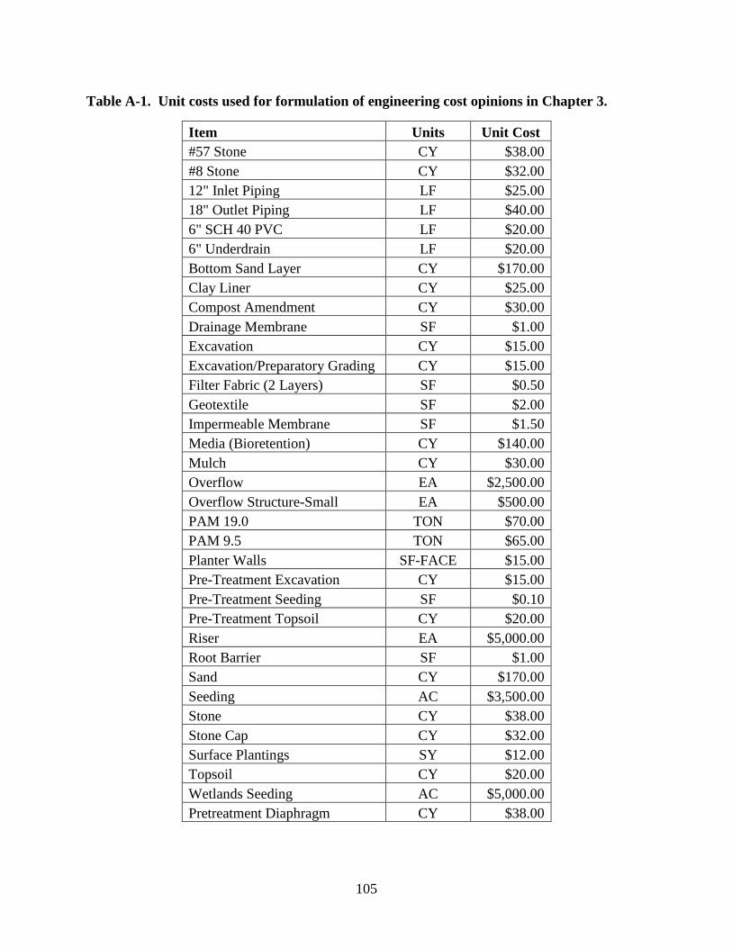
105
Table A-1. Unit costs used for formulation of engineering cost opinions in Chapter 3.
Item Units Unit Cost
#57 Stone CY $38.00
#8 Stone CY $32.00
12" Inlet Piping LF $25.00
18" Outlet Piping LF $40.00
6" SCH 40 PVC LF $20.00
6" Underdrain LF $20.00
Bottom Sand Layer CY $170.00
Clay Liner CY $25.00
Compost Amendment CY $30.00
Drainage Membrane SF $1.00
Excavation CY $15.00
Excavation/Preparatory Grading CY $15.00
Filter Fabric (2 Layers) SF $0.50
Geotextile SF $2.00
Impermeable Membrane SF $1.50
Media (Bioretention) CY $140.00
Mulch CY $30.00
Overflow EA $2,500.00
Overflow Structure-Small EA $500.00
PAM 19.0 TON $70.00
PAM 9.5 TON $65.00
Planter Walls SF-FACE $15.00
Pre-Treatment Excavation CY $15.00
Pre-Treatment Seeding SF $0.10
Pre-Treatment Topsoil CY $20.00
Riser EA $5,000.00
Root Barrier SF $1.00
Sand CY $170.00
Seeding AC $3,500.00
Stone CY $38.00
Stone Cap CY $32.00
Surface Plantings SY $12.00
Topsoil CY $20.00
Wetlands Seeding AC $5,000.00
Pretreatment Diaphragm CY $38.00

106
APPENDIX B: Case Study 1 (used in Chapter 4)

107
Case Study 1 – Small Scale Commercial Development
As part of a conceptual design package, you have been tasked with developing a preliminary
stormwater management plan for a development project located in Loddi, Virginia (fictional).
The parcel area totals 1.64 acres and fronts on First Street. It is expected that any quantity
control required to meet the erosion and channel protection discharge requirements will take
place in an underground detention facility; therefore, the goal for this conceptual design is to
meet stormwater quality compliance only, with additional quantity design being performed later,
during the final design process. The developer is attempting to acquire additional adjacent
acreage for an expanded Phase II, but has been unsuccessful in reaching agreements with the
owners of neighboring parcels at this time.
Table B-1.SCS 24 Hour Rainfall Totals
1 Year 2 Year 10 Year 100 Year 24 Hour Rainfall (in) 2.28 2.76 4.11 6.51
Existing Conditions
The site, totaling 1.64 acres (Figure B-1), is covered primarily with turf and a couple of sparse
trees. Phase I is entirely underlain by HSG B soils. Access into the site will be from First Street
to the east.
Figure B-1. CS-1 – Existing Conditions
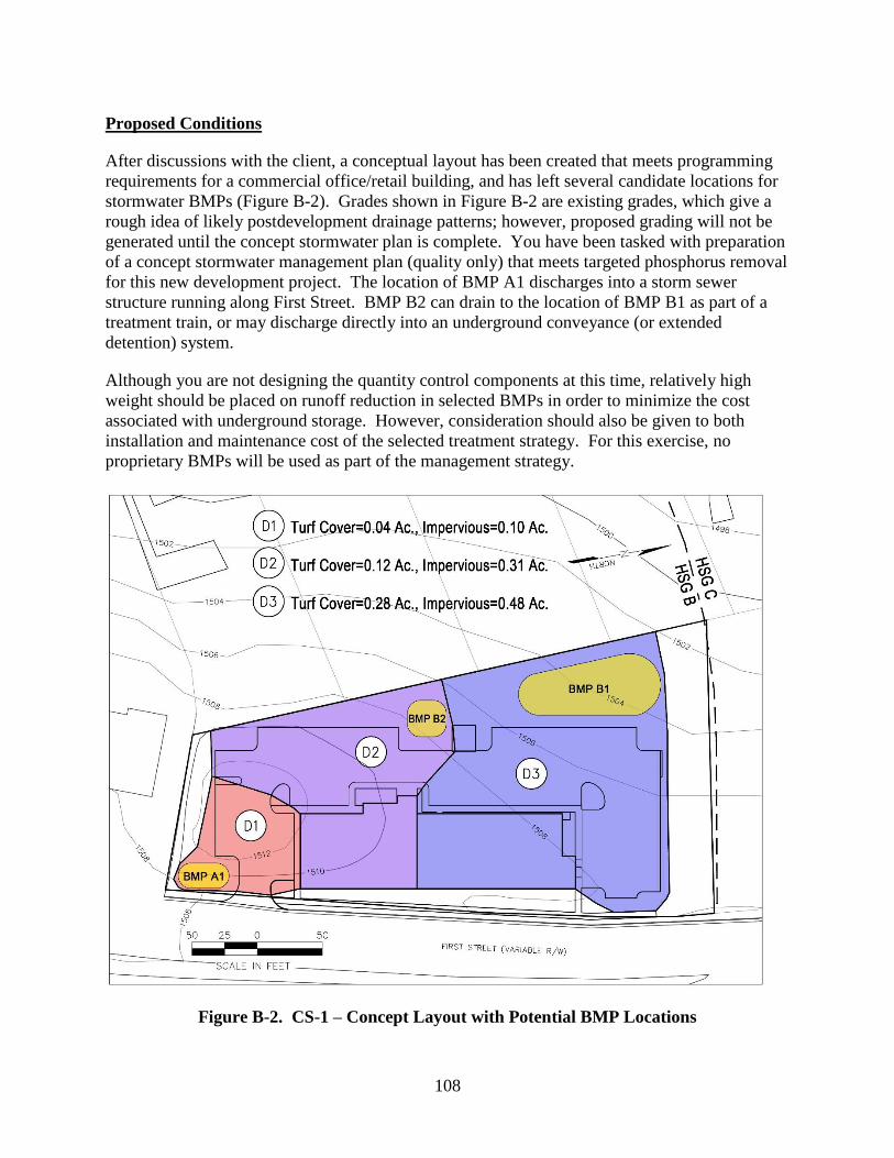
108
Proposed Conditions
After discussions with the client, a conceptual layout has been created that meets programming
requirements for a commercial office/retail building, and has left several candidate locations for
stormwater BMPs (Figure B-2). Grades shown in Figure B-2 are existing grades, which give a
rough idea of likely postdevelopment drainage patterns; however, proposed grading will not be
generated until the concept stormwater plan is complete. You have been tasked with preparation
of a concept stormwater management plan (quality only) that meets targeted phosphorus removal
for this new development project. The location of BMP A1 discharges into a storm sewer
structure running along First Street. BMP B2 can drain to the location of BMP B1 as part of a
treatment train, or may discharge directly into an underground conveyance (or extended
detention) system.
Although you are not designing the quantity control components at this time, relatively high
weight should be placed on runoff reduction in selected BMPs in order to minimize the cost
associated with underground storage. However, consideration should also be given to both
installation and maintenance cost of the selected treatment strategy. For this exercise, no
proprietary BMPs will be used as part of the management strategy.
Figure B-2. CS-1 – Concept Layout with Potential BMP Locations
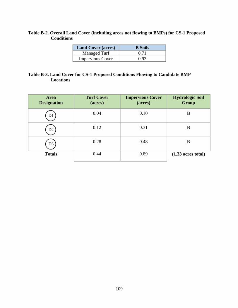
109
Table B-2. Overall Land Cover (including areas not flowing to BMPs) for CS-1 Proposed
Conditions
Land Cover (acres) B Soils
Managed Turf 0.71
Impervious Cover 0.93
Table B-3. Land Cover for CS-1 Proposed Conditions Flowing to Candidate BMP
Locations
Area
Designation
Turf Cover
(acres)
Impervious Cover
(acres)
Hydrologic Soil
Group
0.04 0.10 B
0.12 0.31 B
0.28 0.48 B
Totals 0.44 0.89 (1.33 acres total)
D1
D2
D3

110
APPENDIX C: Case Study 2 (used in Chapter 4)

111
Case Study 2 – Phase II – Mixed Use Development
During construction of Phase I, the developer is finally successful in obtaining additional
adjacent lots, and is ready to move forward with Phase II development. As part of the Phase II
conceptual design package, you have been tasked with developing a preliminary stormwater
management plan for the full build-out of the development, which will include the improvements
you have already designed for Phase I. The locality is requiring a reanalysis of the entire site
area (including Phase I) as a redevelopment scenario, assuming that existing conditions were
those prior to the start of construction on Phase I. Site characteristics for the entire
predevelopment parcel are shown in Figure C-1. It is assumed that virtually all of the 9.65 acres
will be disturbed during construction.
Existing Conditions
As seen in Figure C-1, there are several existing dwellings to the west and one existing small
commercial lot to the north that must be accounted for in the re-development stormwater quality
calculations. There are no forested areas within the boundary of the site. Land coverage data for
existing conditions is summarized in Table C-1.
Figure C-1. CS-2 – Existing Conditions (Prior to Phase I Construction)
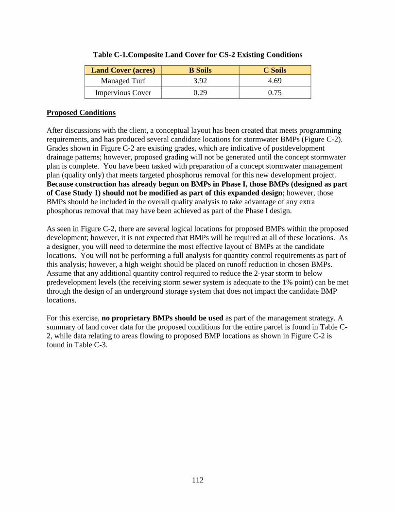
112
Table C-1.Composite Land Cover for CS-2 Existing Conditions
Land Cover (acres) B Soils C Soils
Managed Turf 3.92 4.69
Impervious Cover 0.29 0.75
Proposed Conditions
After discussions with the client, a conceptual layout has been created that meets programming
requirements, and has produced several candidate locations for stormwater BMPs (Figure C-2).
Grades shown in Figure C-2 are existing grades, which are indicative of postdevelopment
drainage patterns; however, proposed grading will not be generated until the concept stormwater
plan is complete. You have been tasked with preparation of a concept stormwater management
plan (quality only) that meets targeted phosphorus removal for this new development project.
Because construction has already begun on BMPs in Phase I, those BMPs (designed as part
of Case Study 1) should not be modified as part of this expanded design; however, those
BMPs should be included in the overall quality analysis to take advantage of any extra
phosphorus removal that may have been achieved as part of the Phase I design.
As seen in Figure C-2, there are several logical locations for proposed BMPs within the proposed
development; however, it is not expected that BMPs will be required at all of these locations. As
a designer, you will need to determine the most effective layout of BMPs at the candidate
locations. You will not be performing a full analysis for quantity control requirements as part of
this analysis; however, a high weight should be placed on runoff reduction in chosen BMPs.
Assume that any additional quantity control required to reduce the 2-year storm to below
predevelopment levels (the receiving storm sewer system is adequate to the 1% point) can be met
through the design of an underground storage system that does not impact the candidate BMP
locations.
For this exercise, no proprietary BMPs should be used as part of the management strategy. A
summary of land cover data for the proposed conditions for the entire parcel is found in Table C-
2, while data relating to areas flowing to proposed BMP locations as shown in Figure C-2 is
found in Table C-3.
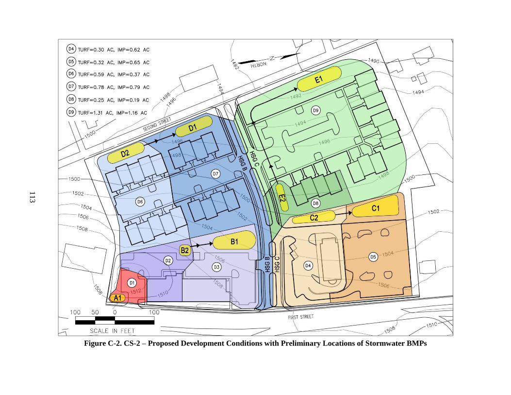
Figure C-2. CS-2 – Proposed Development Conditions with Preliminary Locations of Stormwater BMPs
113
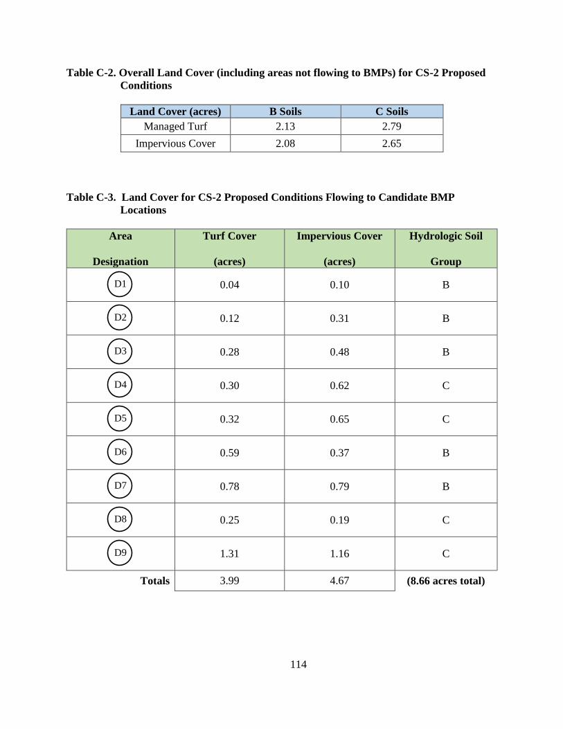
114
Table C-2. Overall Land Cover (including areas not flowing to BMPs) for CS-2 Proposed
Conditions
Land Cover (acres) B Soils C Soils
Managed Turf 2.13 2.79
Impervious Cover 2.08 2.65
Table C-3. Land Cover for CS-2 Proposed Conditions Flowing to Candidate BMP
Locations
Area
Designation
Turf Cover
(acres)
Impervious Cover
(acres)
Hydrologic Soil
Group
0.04 0.10 B
0.12 0.31 B
0.28 0.48 B
0.30 0.62 C
0.32 0.65 C
0.59 0.37 B
0.78 0.79 B
0.25 0.19 C
1.31 1.16 C
Totals 3.99 4.67 (8.66 acres total)
D1
D2
D3
D4
D5
D6
D7
D8
D9

115
APPENDIX D: Case Study Sample Questionnaire

116
Participant Questionnaire (common questions for either tool)
1. How many years of experience do you have performing stormwater computations
related to land development projects?
< 2 years
2 – 4 years
5 – 10 years
> 10 years
2. Approximate the number of projects for which you have used the VRRM spreadsheets
to determine water quality compliance?
< 4
5 - 10
10 - 20
> 20
3. Consider your use of the drainage area tab(s) on the tool you used today. Based on that
experience rate your level of agreement with the following items:
1 Strongly Disagree
2 Somewhat Disagree
3 Neither Agree or Disagree
4 Somewhat
Agree
5 Strongly
Agree
Data entry is easy Adding treatment train
connectivity is easy
Tool allows visualization
of treatment train
connectivity
Tool provides ability to
take into account
constraints at BMP
location
Changing entry to an
alternate BMP is easy
Iterating through multiple
treatment train test
solutions is easy and time
efficient

117
4. Consider your analysis for the case study today. Based on your analysis, rate your
level of agreement with whether or not you actively considered the following criteria
during development of your final solution(s):
1 Strongly Disagree
2 Somewhat Disagree
3 Neither Agree or Disagree
4 Somewhat
Agree
5 Strongly
Agree
Consideration of contributing
drainage area to BMP location
Consideration of physical site
constraints
BMP installation cost BMP maintenance cost Consideration of total volume
(runoff) reduction provided
Consideration of aesthetics
5. What percentage of your time today did you spend on manipulating entries in the
drainage area tab(s) to meet the phosphorus reduction goals?
< 10 minutes
10 – 20 minutes
21 – 30 minutes
31– 45 minutes
> 45 minutes
6. What percentage of your time today did you spend on evaluating results from solution
alternatives?
< 10 minutes
10 – 20 minutes
21 – 30 minutes
31– 45 minutes
> 45 minutes
7. How many alternative solutions were considered?
< 2
2 - 5
6 - 10
> 10

118
8. When developing alternate solutions, which cost factors were considered?
Installation cost
Maintenance cost
Both installation and maintenance cost
Cost was not considered
9. Consider your use of the assigned tool (spreadsheets or VT software today). Indicate
level of agreement with the following statements:
1
Strongly Disagree
2 Somewhat Disagree
3 Neither Agree or Disagree
4 Somewhat
Agree
5 Strongly
Agree
The assigned tool affected the
way I typically approach BMP
design
The tool enhanced my efficiency
in design by simplifying
repetitive tasks
The tool allows me to spend
more time on evaluation of
results rather than on input of
data
The tool allowed me to quickly
consider siting constraints
The tool allowed me to consider
alternatives that I would not
have otherwise considered
The tool allows me to take cost
into account when selecting the
best alternatives
The tool was easy to use The tool will enhance my
effectiveness in providing
services to my clients
The tool is visually appealing

119
APPENDIX E: Raw Data from Case Studies
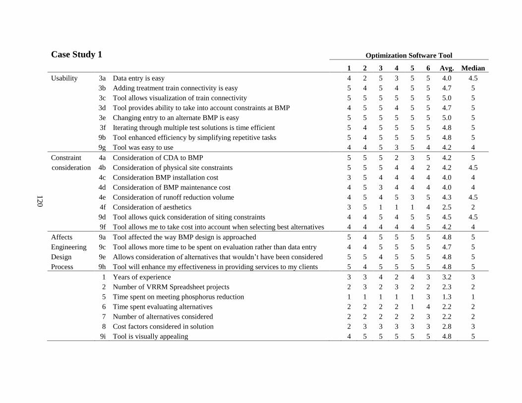
Case Study 1 Optimization Software Tool
1 2 3 4 5 6 Avg. Median
Usability 3a Data entry is easy 4 2 5 3 5 5 4.0 4.5
3b Adding treatment train connectivity is easy 5 4 5 4 5 5 4.7 5
3c Tool allows visualization of train connectivity 5 5 5 5 5 5 5.0 5
3d Tool provides ability to take into account constraints at BMP 4 5 5 4 5 5 4.7 5
3e Changing entry to an alternate BMP is easy 5 5 5 5 5 5 5.0 5
3f Iterating through multiple test solutions is time efficient 5 4 5 5 5 5 4.8 5
9b Tool enhanced efficiency by simplifying repetitive tasks 5 4 5 5 5 5 4.8 5
9g Tool was easy to use 4 4 5 3 5 4 4.2 4
Constraint 4a Consideration of CDA to BMP 5 5 5 2 3 5 4.2 5
consideration 4b Consideration of physical site constraints 5 5 5 4 4 2 4.2 4.5
4c Consideration BMP installation cost 3 5 4 4 4 4 4.0 4
4d Consideration of BMP maintenance cost 4 5 3 4 4 4 4.0 4
4e Consideration of runoff reduction volume 4 5 4 5 3 5 4.3 4.5
4f Consideration of aesthetics 3 5 1 1 1 4 2.5 2
9d Tool allows quick consideration of siting constraints 4 4 5 4 5 5 4.5 4.5
9f Tool allows me to take cost into account when selecting best alternatives 4 4 4 4 4 5 4.2 4
Affects 9a Tool affected the way BMP design is approached 5 4 5 5 5 5 4.8 5
Engineering 9c Tool allows more time to be spent on evaluation rather than data entry 4 4 5 5 5 5 4.7 5
Design 9e Allows consideration of alternatives that wouldn’t have been considered 5 5 4 5 5 5 4.8 5
Process 9h Tool will enhance my effectiveness in providing services to my clients 5 4 5 5 5 5 4.8 5
1 Years of experience 3 3 4 2 4 3 3.2 3
2 Number of VRRM Spreadsheet projects 2 3 2 3 2 2 2.3 2
5 Time spent on meeting phosphorus reduction 1 1 1 1 1 3 1.3 1
6 Time spent evaluating alternatives 2 2 2 2 1 4 2.2 2
7 Number of alternatives considered 2 2 2 2 2 3 2.2 2
8 Cost factors considered in solution 2 3 3 3 3 3 2.8 3
9i Tool is visually appealing 4 5 5 5 5 5 4.8 5
120

Case Study 1 VRRM Spreadsheets
1 2 3 4 5 Avg. Median
Usability 3a Data entry is easy 2 5 3 4 4 3.6 4
3b Adding treatment train connectivity is easy 4 4 3 4 4 3.8 4
3c Tool allows visualization of train connectivity 2 1 1 4 2 2 2
3d Tool provides ability to take into account constraints at BMP 1 1 1 2 2 1.4 1
3e Changing entry to an alternate BMP is easy 2 5 2 3 3 3 3
3f Iterating through multiple test solutions is time efficient 1 1 2 1 3 1.6 1
9b Tool enhanced efficiency by simplifying repetitive tasks 2 1 2 2 2 1.8 2
9g Tool was easy to use 4 5 3 4 3 3.8 4
Constraint 4a Consideration of CDA to BMP 5 5 2 4 3 3.8 4
consideration 4b Consideration of physical site constraints 4 5 4 4 4 4.2 4
4c Consideration BMP installation cost 3 4 4 1 2 2.8 3
4d Consideration of BMP maintenance cost 3 4 3 1 2 2.6 3
4e Consideration of runoff reduction volume 4 5 5 1 4 3.8 4
4f Consideration of aesthetics 3 5 4 1 3 3.2 3
9d Tool allows quick consideration of siting constraints 1 1 2 2 2 1.6 2
9f Tool allows me to take cost into account when selecting best alternatives 1 1 1 1 2 1.2 1
Affects 9a Tool affected the way BMP design is approached 2 5 4 3 4 3.6 4
Engineering 9c Tool allows more time to be spent on evaluation rather than data entry 1 1 2 2 3 1.8 2
Design 9e Allows consideration of alternatives that wouldn’t have been considered 1 1 1 2 1 1.2 1
Process 9h Tool will enhance my effectiveness in providing services to my clients 2 3 3 2 3 2.6 3
1 Years of experience 2 2 4 4 3 3 2.5
2 Number of VRRM Spreadsheet projects 2 4 3 3 3 3 3
5 Time spent on meeting phosphorus reduction 2 1 1 1 1 1.2 1
6 Time spent evaluating alternatives 1 2 1 1 1 1.2 1
7 Number of alternatives considered 2 1 2 2 2 1.8 2
8 Cost factors considered in solution 1 3 1 4 1 2 2
9i Tool is visually appealing 1 3 2 3 4 2.6 3
121
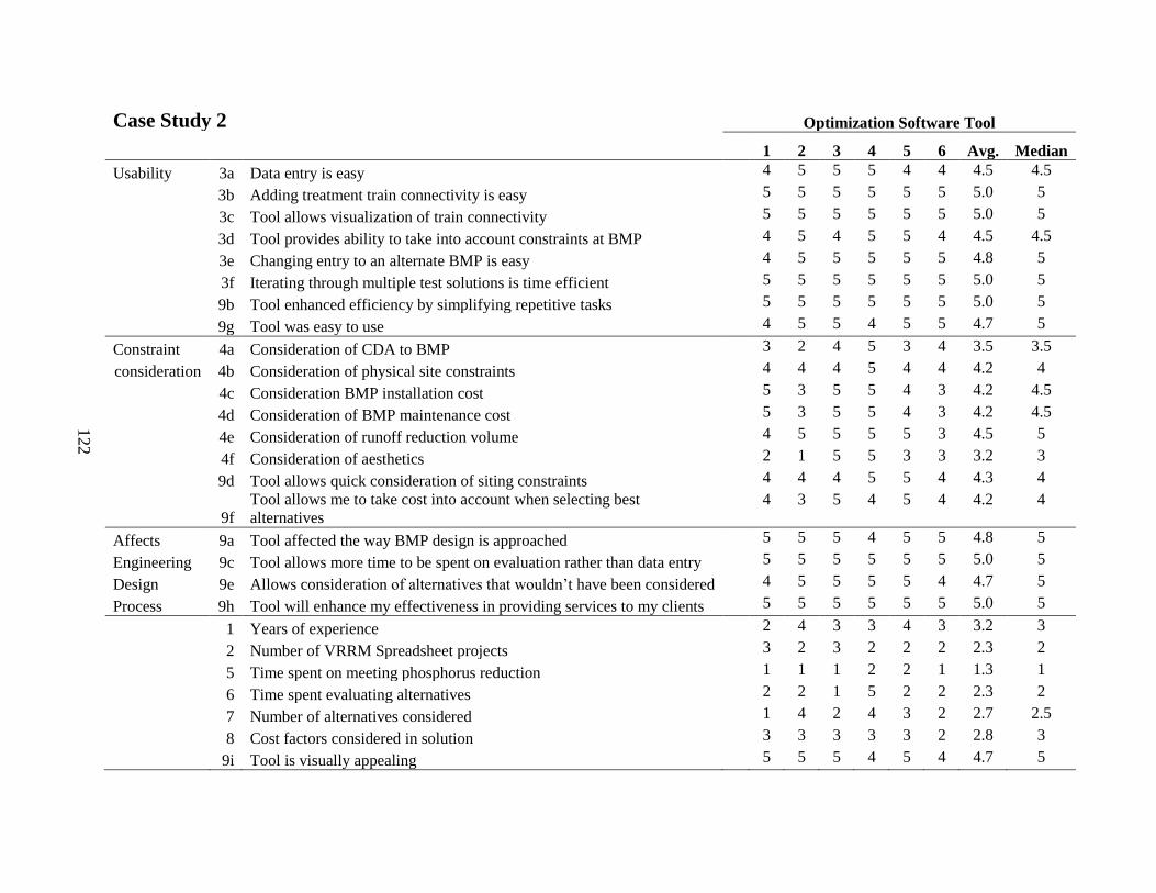
Case Study 2 Optimization Software Tool
1 2 3 4 5 6 Avg. Median
Usability 3a Data entry is easy 4 5 5 5 4 4 4.5 4.5
3b Adding treatment train connectivity is easy 5 5 5 5 5 5 5.0 5
3c Tool allows visualization of train connectivity 5 5 5 5 5 5 5.0 5
3d Tool provides ability to take into account constraints at BMP 4 5 4 5 5 4 4.5 4.5
3e Changing entry to an alternate BMP is easy 4 5 5 5 5 5 4.8 5
3f Iterating through multiple test solutions is time efficient 5 5 5 5 5 5 5.0 5
9b Tool enhanced efficiency by simplifying repetitive tasks 5 5 5 5 5 5 5.0 5
9g Tool was easy to use 4 5 5 4 5 5 4.7 5
Constraint 4a Consideration of CDA to BMP 3 2 4 5 3 4 3.5 3.5
consideration 4b Consideration of physical site constraints 4 4 4 5 4 4 4.2 4
4c Consideration BMP installation cost 5 3 5 5 4 3 4.2 4.5
4d Consideration of BMP maintenance cost 5 3 5 5 4 3 4.2 4.5
4e Consideration of runoff reduction volume 4 5 5 5 5 3 4.5 5
4f Consideration of aesthetics 2 1 5 5 3 3 3.2 3
9d Tool allows quick consideration of siting constraints 4 4 4 5 5 4 4.3 4
9f
Tool allows me to take cost into account when selecting best
alternatives
4 3 5 4 5 4 4.2 4
Affects 9a Tool affected the way BMP design is approached 5 5 5 4 5 5 4.8 5
Engineering 9c Tool allows more time to be spent on evaluation rather than data entry 5 5 5 5 5 5 5.0 5
Design 9e Allows consideration of alternatives that wouldn’t have been considered 4 5 5 5 5 4 4.7 5
Process 9h Tool will enhance my effectiveness in providing services to my clients 5 5 5 5 5 5 5.0 5
1 Years of experience 2 4 3 3 4 3 3.2 3
2 Number of VRRM Spreadsheet projects 3 2 3 2 2 2 2.3 2
5 Time spent on meeting phosphorus reduction 1 1 1 2 2 1 1.3 1
6 Time spent evaluating alternatives 2 2 1 5 2 2 2.3 2
7 Number of alternatives considered 1 4 2 4 3 2 2.7 2.5
8 Cost factors considered in solution 3 3 3 3 3 2 2.8 3
9i Tool is visually appealing 5 5 5 4 5 4 4.7 5
122

Case Study 2 VRRM Spreadsheets
1 2 3 4 5 Avg. Median
Usability 3a Data entry is easy 5 2 1 2 2 2.4 2
3b Adding treatment train connectivity is easy 4 2 4 3 2 3 3
3c Tool allows visualization of train connectivity 1 2 1 2 1 1.4 1
3d Tool provides ability to take into account constraints at BMP 1 2 1 2 1 1.4 1
3e Changing entry to an alternate BMP is easy 5 2 1 1 2 2.2 2
3f Iterating through multiple test solutions is time efficient 1 2 1 2 1 1.4 1
9b Tool enhanced efficiency by simplifying repetitive tasks 1 2 1 2 2 1.6 2
9g Tool was easy to use 5 3 2 3 2 3 3
Constraint 4a Consideration of CDA to BMP -- 4 4 2 4 3.5 4
consideration 4b Consideration of physical site constraints -- 4 4 2 4 3.5 4
4c Consideration BMP installation cost -- 2 2 3 4 2.75 2.5
4d Consideration of BMP maintenance cost -- 2 2 3 4 2.75 2.5
4e Consideration of runoff reduction volume -- 4 4 4 2 3.5 4
4f Consideration of aesthetics -- 2 2 3 3 2.5 2.5
9d Tool allows quick consideration of siting constraints 1 2 1 2 1 1.4 1
9f Tool allows me to take cost into account when selecting best alternatives 1 1 1 2 1 1.2 1
Affects 9a Tool affected the way BMP design is approached 3 2 2 4 2 2.6 2
Engineering 9c Tool allows more time to be spent on evaluation rather than data entry 3 2 1 2 2 2 2
Design 9e Allows consideration of alternatives that wouldn’t have been considered 1 2 3 2 2 2 2
Process 9h Tool will enhance my effectiveness in providing services to my clients 1 3 3 3 2 2.4 3
1 Years of experience 2 4 3 3 4 3.2 3
2 Number of VRRM Spreadsheet projects 4 3 2 3 3 3 3
5 Time spent on meeting phosphorus reduction 1 2 2 2 1 1.6 2
6 Time spent evaluating alternatives 4 1 2 3 2 2.4 2.5
7 Number of alternatives considered 2 3 2 4 2 2.6 2.5
8 Cost factors considered in solution 3 4 4 4 3 3.6 4
9i Tool is visually appealing 3 3 1 3 2 2.4 3
123