Urban Hydrology

7/30/2019 Urban Hydrology

http://slidepdf.com/reader/full/urbanhydrology 1/39

3-1

Figure 3-1. Example IDF curve.

3. URBAN HYDROLOGIC PROCEDURES

This section provides an overview of hydrologic methods and procedures commonly used inurban highway drainage design. Much of the information contained in this section wascondensed from Hydraulic Design Series 2, (HDS-2) Hydrology(6). The presentation here isintended to provide the reader with an introduction to the methods and procedures, their data

requirements, and their limitations. Most of these procedures can be applied using commonlyavailable computer programs. HDS-2 contains additional information and detail on the methodsdescribed.

3.1 Rainfall (Precipitation)

Rainfall, along with watershed characteristics, determines the flood flows upon which stormdrainage design is based. The following sections describe three representations of rainfallwhich can be used to derive flood flows: constant rainfall intensity, dynamic rainfall, andsynthetic rainfall events.

3.1.1 Constant Rainfall Intensity

Although rainfall intensity varies duringprecipitation events, many of theprocedures used to derive peak flow arebased on an assumed constant rainfallintensity. Intensity is defined as the rate of rainfall and is typically given in units of millimeters per hour (inches per hour).

Intensity-Duration-Frequency curves (IDF

curves) have been developed for many jurisdictions throughout the United Statesthrough frequency analysis of rainfall eventsfor thousands of rainfall gages. The IDFcurve provides a summary of a site's rainfallcharacteristics by relating storm durationand exceedence probability (frequency) torainfall intensity (assumed constant over theduration). Figure 3-1 illustrates an exampleIDF curve. To interpret an IDF curve, findthe rainfall duration along the X-axis, govertically up the graph until reaching the

proper return period, then go horizontally tothe left and read the intensity off of the Y-axis. Regional IDF curves are available inmost highway agency drainage manuals. If the IDF curves are not available, thedesigner needs to develop them on a project by project basis.



3-2

Figure 3-2. Example mass rainfall curve and corresponding hyetography.

3.1.2 Dynamic Rainfall (Hyetograph)

In any given storm, the instantaneous intensity is the slope of the mass rainfall curve at aparticular time. The mass rainfall curve is simply the cumulative precipitation which has fallenup to a specific time. For hydrologic analysis, it is desirable to divide the storm into convenienttime increments and to determine the average intensity over each of the selected periods.

These results are then plotted as rainfall hyetographs, an example of which is presented infigure 3-2. Hyetographs provide greater precision than a constant rainfall intensity by specifyingthe precipitation variability over time, and are used in conjunction with hydrographic (rather thanpeak flow) methods. Hyetographs allow for simulation of actual rainfall events which canprovide valuable information on the relative flood risks of different events and, perhaps,calibration of hydrographic models. Hyetographs of actual storms are often available from theNational Climatic Data Center, which is part of the National Oceanic and Atmospheric

Administration (NOAA).

3.

1.

3Sy

nt

he

tic

Ra

inf

all

Ev

en

ts

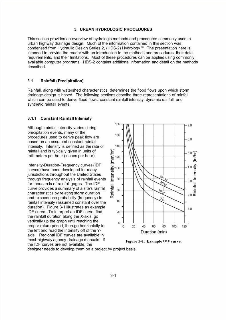
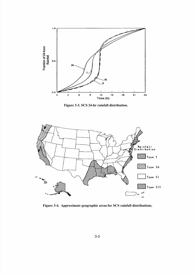
Drainage design is usually based on synthetic rather than actual rainfall events. The SCS 24-hour rainfall distributions are the most widely used synthetic hyetographs. These rainfalldistributions were developed by the U.S. Department of Agriculture, Soil Conservation Service(SCS) (13) which is now known as the Natural Resources Conservation Service (NRCS). TheSCS 24-hour distributions incorporate the intensity-duration relationship for the design returnperiod. This approach is based on the assumption that the maximum rainfall for any durationwithin the 24-hour duration should have the same return period. For example, a 10-year, 24-hour design storm would contain the 10-year rainfall depths for all durations up to 24 hour asderived from IDF curves. SCS developed four synthetic 24-hour rainfall distributions as shownin figure 3-3; approximate geographic boundaries for each storm distribution are shown in figure3-4.

HDS-2 provides a tabular listing of the SCS distributions, which are shown in figure 3-3. Although these distributions do not agree exactly with IDF curves for all locations in the regionfor which they are intended, the differences are within the accuracy limits of the rainfall depthsread from the Weather Bureau's Rainfall Frequency Atlases (6).



3-3

Figure 3-4. Approximate geographic areas for SCS rainfall distributions.

Figure 3-3. SCS 24-hr rainfall distribution.



3-4

Figure 3-5. Log Pearson Type III distribution analysis, Medina River,

Texas.

3.2 Determination of Peak Flow Rates

Peak flows are generally adequate for design and analysis of conveyance systems such asstorm drains or open channels. However, if the design or analysis must include flood routing(e.g., storage basins or complex conveyance networks), a flood hydrograph is required. Thissection discusses methods used to derive peak flows for both gaged and ungaged sites.

3.2.1 Stochastic Methods

Stochastic methods, or frequency analysis, can be used to evaluate peak flows where adequategaged streamflow data exist. Frequency distributions are used in the analysis of hydrologicdata and include the normal distribution, the log-normal distribution, the Gumbel extreme valuedistribution, and the log-Pearson Type III distribution. The log-Pearson Type III distribution is athree-parameter gamma distribution with a logarithmic transform of the independent variable. Itis widely used for flood analyses because the data quite frequently fit the assumed population.It is this flexibility that led the U.S. Water Resources Council to recommend its use as thestandard distribution for flood frequency studies by all U.S. Government agencies. Figure 3-5

presents an example of a log-Pearson Type III distribution frequency curve (6). Stochasticmethods are not commonly used in urban drainage design due to the lack of adequatestreamflow data. Consult HDS-2(6) for additional information on stochastic methods.



3-5

Weighted C j (Cx Ax )

Atotal

(3-2)

3.2.2 Rational Method

One of the most commonly used equations for the calculation of peak flow from small areas isthe Rational formula, given as:

where:

Q = Flow, m3/s (ft3/s)C = dimensionless runoff coefficientI = rainfall intensity, mm/hr (in/hr)

A = drainage area, hectares, ha (acres)Ku = units conversion factor equal to 360 (1.0 in English Units)

Assumptions inherent in the Rational formula are as follows (6):

• Peak flow occurs when the entire watershed is contributing to the flow.

• Rainfall intensity is the same over the entire drainage area.

• Rainfall intensity is uniform over a time duration equal to the time of concentration, tc. Thetime of concentration is the time required for water to travel from the hydraulically mostremote point of the basin to the point of interest.

• Frequency of the computed peak flow is the same as that of the rainfall intensity, i.e., the10-year rainfall intensity is assumed to produce the 10-year peak flow.

• Coefficient of runoff is the same for all storms of all recurrence probabilities.

Because of these inherent assumptions, the Rational formula should only be applied todrainage areas smaller than 80 ha (200 ac) (8).

3.2.2.1 Runoff Coefficient

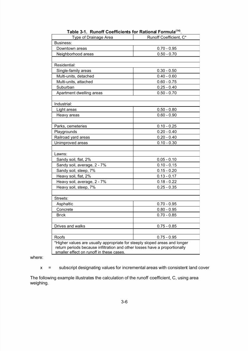
The runoff coefficient, C, in equation 3-1 is a function of the ground cover and a host of other hydrologic abstractions. It relates the estimated peak discharge to a theoretical maximum of 100 percent runoff. Typical values for C are given in table 3-1. If the basin contains varying

amounts of different land cover or other abstractions, a composite coefficient can be calculatedthrough areal weighing as follows (6):

Q CIAKu

(3-1)



3-6

Table 3-1. Runoff Coefficients for Rational Formula(14).

Type of Drainage Area Runoff Coefficient, C*

Business:

Downtown areas 0.70 - 0.95

Neighborhood areas 0.50 - 0.70

Residential:

Single-family areas 0.30 - 0.50

Multi-units, detached 0.40 - 0.60

Multi-units, attached 0.60 - 0.75

Suburban 0.25 - 0.40

Apartment dwelling areas 0.50 - 0.70

Industrial:

Light areas 0.50 - 0.80

Heavy areas 0.60 - 0.90

Parks, cemeteries 0.10 - 0.25

Playgrounds 0.20 - 0.40

Railroad yard areas 0.20 - 0.40

Unimproved areas 0.10 - 0.30

Lawns:

Sandy soil, flat, 2% 0.05 - 0.10

Sandy soil, average, 2 - 7% 0.10 - 0.15

Sandy soil, steep, 7% 0.15 - 0.20

Heavy soil, flat, 2% 0.13 - 0.17

Heavy soil, average, 2 - 7% 0.18 - 0.22

Heavy soil, steep, 7% 0.25 - 0.35

Streets:

Asphaltic 0.70 - 0.95

Concrete 0.80 - 0.95

Brick 0.70 - 0.85

Drives and walks 0.75 - 0.85

Roofs 0.75 - 0.95

*Higher values are usually appropriate for steeply sloped areas and longer

return periods because infiltration and other losses have a proportionallysmaller effect on runoff in these cases.

where:

x = subscript designating values for incremental areas with consistent land cover

The following example illustrates the calculation of the runoff coefficient, C, using areaweighing.



3-7

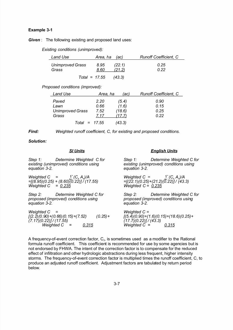
Example 3-1

Given : The following existing and proposed land uses:

Existing conditions (unimproved):

Land Use Area, ha (ac) Runoff Coefficient, C

Unimproved GrassGrass

8.95 (22.1)8.60 (21.2)

0.25 0.22

Total = 17.55 (43.3)

Proposed conditions (improved):

Land Use Area, ha (ac) Runoff Coefficient, C

Paved LawnUnimproved Grass

Grass

2.20 (5.4)0.66 (1.6)7.52 (18.6)

7.17 (17.7)

0.90 0.15 0.25

0.22

Total = 17.55 (43.3)

Find: Weighted runoff coefficient, C, for existing and proposed conditions.

Solution:

SI Units

Step 1: Determine Weighted C for existing (unimproved) conditions using equation 3-2.

Weighted C = 3 (C x A x )/A=[(8.95)(0.25) + (8.60)(0.22)] / (17.55)Weighted C = 0.235

Step 2: Determine Weighted C for proposed (improved) conditions using equation 3-2.

Weighted C =[(2.2)(0.90)+(0.66)(0.15)+(7.52) (0.25)+(7.17)(0.22)] / (17.55)

Weighted C = 0.315

English Units

Step 1: Determine Weighted C for existing (unimproved) conditions using equation 3-2.

Weighted C = 3 (C x A x )/A=[(22.1)(0.25)+(21.2)(0.22)] / (43.3)Weighted C = 0.235

Step 2: Determine Weighted C for proposed (improved) conditions using equation 3-2.

Weighted C =[(5.4)(0.90)+(1.6)(0.15)+(18.6)(0.25)+(17.7)(0.22)] / (43.3)Weighted C = 0.315

A frequency-of-event correction factor, Cf , is sometimes used as a modifier to the Rationalformula runoff coefficient. This coefficient is recommended for use by some agencies but isnot endorsed by FHWA. The intent of the correction factor is to compensate for the reducedeffect of infiltration and other hydrologic abstractions during less frequent, higher intensitystorms. The frequency-of-event correction factor is multiplied times the runoff coefficient, C, toproduce an adjusted runoff coefficient. Adjustment factors are tabulated by return periodbelow.



3-8

Tti Ku

I 0.4n L

S

0.6

(3-3)

Tr < 25 years Cf = 1.00Tr = 25 years Cf = 1.10Tr = 50 years Cf = 1.20Tr = 100 years Cf = 1.25

3.2.2.2 Rainfall Intensity

Rainfall intensity, duration, and frequency curves are necessary to use the Rational method.Regional IDF curves are available in most state highway agency manuals and are also availablefrom the National Oceanic and Atmospheric Administration (NOAA). Again, if the IDF curvesare not available, they need to be developed.

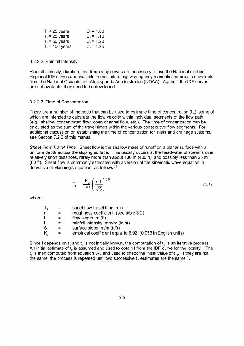
3.2.2.3 Time of Concentration

There are a number of methods that can be used to estimate time of concentration (tc), some of which are intended to calculate the flow velocity within individual segments of the flow path

(e.g., shallow concentrated flow, open channel flow, etc.). The time of concentration can becalculated as the sum of the travel times within the various consecutive flow segments. For additional discussion on establishing the time of concentration for inlets and drainage systems,see Section 7.2.2 of this manual.

Sheet Flow Travel Time. Sheet flow is the shallow mass of runoff on a planar surface with auniform depth across the sloping surface. This usually occurs at the headwater of streams over relatively short distances, rarely more than about 130 m (400 ft), and possibly less than 25 m(80 ft). Sheet flow is commonly estimated with a version of the kinematic wave equation, aderivative of Manning's equation, as follows (6):

where:

Tti = sheet flow travel time, minn = roughness coefficient. (see table 3-2)L = flow length, m (ft)I = rainfall intensity, mm/hr (in/hr)S = surface slope, m/m (ft/ft)Ku = empirical coefficient equal to 6.92 (0.933 in English units)

Since I depends on tc and tc is not initially known, the computation of tc is an iterative process. An initial estimate of tc is assumed and used to obtain I from the IDF curve for the locality. Thetc is then computed from equation 3-3 and used to check the initial value of t c. If they are notthe same, the process is repeated until two successive tc estimates are the same(6).



3-9

Table 3-2. Manning's Roughness Coefficient (n) for Overland Sheet Flow(6).

Surface Description n

Smooth asphalt 0.011

Smooth concrete 0.012

Ordinary concrete lining 0.013

Good wood 0.014

Brick with cement mortar 0.014

Vitrified clay 0.015

Cast iron 0.015

Corrugated metal pipe 0.024

Cement rubble surface 0.024

Fallow (no residue) 0.05

Cultivated soils

Residue cover # 20% 0.06

Residue cover > 20% 0.17

Range (natural) 0.13

Grass

Short grass prairie 0.15

Dense grasses 0.24

Bermuda grass 0.41

Woods*

Light underbrush 0.40

Dense underbrush 0.80

*When selecting n, consider cover to a height of about 30 mm. This isonly part of the plant cover that will obstruct sheet flow.



3-10

V

Ku k S

0.5

p (3-4)

V

Ku

nR 2/3 S 1/2 (3-5)

Tti L

60V(3-6)

Shallow Concentrated Flow Velocity. After short distances of at most 130 m (400 ft), sheet flowtends to concentrate in rills and then gullies of increasing proportions. Such flow is usually referredto as shallow concentrated flow. The velocity of such flow can be estimated using a relationshipbetween velocity and slope as follows (6):

where:

Ku = 1.0 (3.28 in English units)V = velocity, m/s (ft/s)k = intercept coefficient (table 3-3)Sp = slope, percent

Open Channel and Pipe Flow Velocity. Flow in gullies empties into channels or pipes. Openchannels are assumed to begin where either the blue stream line shows on USGS quadranglesheets or the channel is visible on aerial photographs. Cross-section geometry and roughness

should be obtained for all channel reaches in the watershed. Manning's equation can be used toestimate average flow velocities in pipes and open channels as follows:

where:

n = roughness coefficient (see table 3-4)V = velocity, m/s (ft/s)R = hydraulic radius (defined as the flow area divided by the wetted perimeter),

m (ft)S = slope, m/m (ft/ft)Ku = units conversion factor equal to 1 (1.49 in English units)

For a circular pipe flowing full, the hydraulic radius is one-fourth of the diameter. For a widerectangular channel (W > 10 d), the hydraulic radius is approximately equal to the depth. Thetravel time is then calculated as follows:

where:

Tti = travel time for segment i, minL = flow length for segment i, m (ft)V = velocity for segment i, m/s (ft/s)



3-11

Tt i Ku

I 0.4n L

S

0.6

Table 3-3. Intercept Coefficients for Velocity vs. Slope Relationship of Equation 3-4(6).

Land Cover/Flow Regime k

Forest with heavy ground litter; hay meadow (overland flow) 0.076

Trash fallow or minimum tillage cultivation; contour or strip

cropped; woodland (overland flow)

0.152

Short grass pasture (overland flow) 0.213

Cultivated straight row (overland flow) 0.274

Nearly bare and untilled (overland flow); alluvial fans in westernmountain regions

0.305

Grassed waterway (shallow concentrated flow) 0.457

Unpaved (shallow concentrated flow) 0.491

Paved area (shallow concentrated flow); small upland gullies 0.619

Example 3-2

Given: The following flow path characteristics:

Flow Segment Length (m) (ft) Slope (m/m)(ft/ft) Segment Description

1 (sheet flow)2 (shallow con.)3 (Flow inconduit)

68 22379 259

146 479

0.005 0.006 0.008

Bermuda grassGrassed waterway 380 mm (15 in ) concrete

pipe

Find: Time of concentration, t c , for the area.

Solution:

SI Units

Step 1. Calculate time of concentration for each segment using the 10 - year IDF curve.

Segment 1

Obtain Manning's n roughness coefficient from Table 3-2:n = 0.41

Determine the sheet flow travel time using equation 3-3:

S i

n c e I i sbeing sought and is also in the equation, an iterative approach must be used. From experience,estimate a time of concentration and read a rainfall intensity from the appropriate IDF curve. In thisexample, try a time of concentration of 30 minutes and read from the IDF curve in Figure 3-1 anintensity of 90 mm/hr. Now use equation 3-3 to see how good the 30 minute estimate was.



3-12

First, solve the equation in terms of I.

T t1 = [6.92/(I)0.4 ] [(0.41)(68)/(0.005)0.5 ] 0.6 = (249.8)/ I 0.4.

Insert 90 mm for I, one gets 41.3 min. Since 41.3 > the assumed 30 min, try the

intensity for 41 minutes from Figure 3-1 which is 72 mm/hr.

Using 72 mm, one gets 45.2 min. Repeat the process with 70 mm/hr for 45 min and a time of 45.7 min was found. This value is close to the 45.2 min.

Use 46 minutes for segment 1.

Segment 2

Obtain intercept coefficient, k, from table 3-3:k = 0.457 & Ku = 1.0

Determine the concentrated flow velocity from equation 3-4:V = Ku k S p

0.5 = (1.0)(0.457)(0.6)0.5 = 0.35 m/s

Determine the travel time from equation 3-6:T t2 = L/(60 V) = 79/[(60)(0.35)] = 3.7 min

Segment 3

Obtain Manning's n roughness coefficient from table 3-4:n = 0.011

Determine the pipe flow velocity from equation 3-5 assuming full flow for this exampleV = (1.0/0.011)(0.38/4)0.67 (0.008)0.5 = 1.7 m/s


Step 2. Determine the total travel time by summing the individual travel times:

t c = T t1 + T t2 + T t3 = 46.0 + 3.7 + 1.4 = 51.1 min; use 51 minutes

English Units

Step 1. Calculate time of concentration for each segment.

Segment 1

Obtain Manning's n roughness coefficient from Table 3-2:n = 0.41



3-13

Tt i Ku

I 0.4

n L

S

0.6

Determine the sheet Flow travel time using equation 3-3:

Since I is being sought and is also in the equation, an iterative approach must be used.From experience, estimate a time of concentration and read a rainfall intensity from theappropriate IDF curve. In this example, try a time of concentration of 30 minutes and read from the IDF curve in Figure 3-1 an intensity of 3.4 in/hr Now use equation 3-3 tosee how good the 30 minute estimate was.

First, solve the equation in terms of I.

T t1 = [0.933/(I)0.4 ] [(0.41)(223)/(0.005)0.5 ] 0.6 = (68.68)/ I 0.4.

Insert 3.4 in/hr for I, one gets 42.1 min. Since 42.1> the assumed 30 min, try theintensity for 42 minutes from Figure 3-1 which is 2.8 in/hr.

Using 2.8 in/hr., one gets 45.4 min. Repeat the process with 2.7 in/hr for 45 min and atime of 46.2 was found. This value is close to the 45.2 min.

Use 46 minutes for segment 1.

Segment 2

Obtain intercept coefficient, k, from table 3-3:k = 0.457 & Ku = 3.281

Determine the concentrated Flow velocity from equation 3-4:V = Ku k S p0.5 = (3.281) (0.457)(0.6)0.5 = 1.16 ft/s


Segment 3

Obtain Manning's n roughness coefficient from table 3-4:n = 0.011

Determine the pipe Flow velocity from equation 3-5 ( assuming full Flow)V = (1.49/0.011)(1.25/4)0.67 (0.008)0.5 = 5.58 ft/s


Step 2. Determine the total travel time by summing the individual travel times:

t c = T t1 + T t2 + T t3 = 46.0 + 3.7 + 1.4 = 51.1 min; use 51 minutes



3-14

Table 3-4. Values of Manning's Coefficient (n) for Channels and Pipes(15).

Conduit Material Manning's n*

Closed Conduits

Asbestos-cement pipe 0.011 0.015

Brick 0.013 - 0.017Cast iron pipe

Cement-lined and seal coated 0.011 - 0.015

Concrete (monolithic) 0.012 - 0.014

Concrete pipe 0.011 - 0.015

Corrugated-metal pipe - 13 mm by 64 mm (½ inch by 2 ½ inch) corrugations

Plain 0.022 - 0.026

Paved invert 0.018 - 0.022

Spun asphalt lines 0.011 - 0.015

Plastic pipe (smooth) 0.011 - 0.015

Vitrified clay

Pipes 0.011 - 0.015

Liner plates 0.013 - 0.017

Open Channels

Lined channels

Asphalt 0.013 - 0.017

Brick 0.012 - 0.018

Concrete 0.011 - 0.020

Rubble or riprap 0.020 - 0.035Vegetal 0.030 - 0.400

Excavated or dredged

Earth, straight and uniform 0.020 - 0.030

Earth, winding, fairly uniform 0.025 - 0.040

Rock 0.030 - 0.045

Unmaintained 0.050 - 0.140

Natural channels (minor streams, top width at flood stage <30 m (100 ft))

Fairly regular section 0.030 - 0.070

Irregular section with pools 0.040 - 0.100

*Lower values are usually for well-constructed and maintained (smoother) pipesand channels.



3-15

Example 3-3

Given: Land use conditions from example 3-1 and the following times of concentration:

Time of concentration

t c (min)

Weighted C

(from example 3-1)Existing condition (unimproved) 88 0.235

Proposed condition (improved) 66 0.315

Area = 17.55 ha (43.36 acres)

Find: The 10-year peak flow using the Rational Formula and the IDF Curve shown in figure 3-1.

Solution:SI Units

Step 1. Determine rainfall intensity, I, fromthe 10-year IDF curve for each time of concentration.

Rainfall intensity, I Existing condition (unimproved) 48 mm/hr

Proposed condition (improved)58 mm/hr

Step 2. Determine peak flow rate, Q.

Existing condition (unimproved):Q = CIA / Ku

= (0.235)(48)(17.55)/360 = 0.55 m3 /s

Proposed condition (improved):Q = CIA / Ku

= (0.315)(58)(17.55)/360 = 0.89 m3 /s

English Units

Step 1. Determine rainfall intensity, I, fromthe 10-year IDF curve for each time of concentration.

Rainfall intensity, I Existing condition (unimproved) 1.9in/hr

Proposed condition (improved) 2.3in/hr

Step 2. Determine peak flow rate, Q.

Existing condition (unimproved):Q = CIA / Ku

= (0.235)(1.9)(43.3)/1= 19.3 ft 3 /s

Proposed condition (improved):Q = CIA / Ku

= (0.315)(2.3)(43.3)/1= 31.4 ft 3 /s

Reference 6 contains additional information on the Rational method.



3-16

RQT a A b B c C d (3-7)

3.2.3 USGS Regression Equations

Regression equations are commonly used for estimating peak flows at ungaged sites or sites withlimited data. The United States Geological Survey (USGS) has developed and compiled regionalregression equations which are included in a computer program called the National FloodFrequency program (NFF). NFF allows quick and easy estimation of peak flows throughout the

United States(15)

. All the USGS regression equations were developed using dependent variablesin English units. Therefore, SI unit information is not provided for this section. Local equations maybe available which provide better correspondence to local hydrology than the regional equationsfound in NFF.

3.2.3.1 Rural Equations

The rural equations are based on watershed and climatic characteristics within specific regions of each state that can be obtained from topographic maps, rainfall reports, and atlases. Theseregression equations are generally of the following form:

where:

RQT = T-year rural peak flowa = regression constantb,c,d = regression coefficients

A,B,C = basin characteristics

Through a series of studies conducted by the USGS, State Highway, and other agencies, ruralequations have been developed for all states. These equations are presented in reference 15,

which has a companion software package to implement these equations. These equations shouldnot be used where dams and other hydrologic modifications have a significant effect on peak flows.Many other limitations are presented in reference 15.

3.2.3.2 Urban Equations

Rural peak flow can be converted to urban peak flows with the seven-parameter Nationwide Urbanregression equations developed by USGS. These equations are shown in table 3-5. (16) A three-parameter equation has also been developed, but the seven-parameter equation is implementedin NFF. The urban equations are based on urban runoff data from 269 basins in 56 cities and 31states. These equations have been thoroughly tested and proven to give reasonable estimatesof peak flows having recurrence intervals between 2 and 500 yrs. Subsequent testing at 78

additional sites in the southeastern United States verified the adequacy of the equations (16). Whilethese regression equations have been verified, errors may still be on the order of 35 to 50 percentwhen compared to field measurements.



3-17

Table 3-5. Nationwide Urban Equations Developed by USGS(17).

UQ2 = 2.35 As.41SL.17(RI2 + 3)2.04(ST + 8)-.65(13 - BDF)-.32IAs

.15RQ2.47 (3-8)


.11RQ5.54 (3-9)


.09RQ10.58 (3-10)

UQ25 = 2.78 As.31

SL.15

(RI2 + 3)1.76

(ST + 8)-.55

(13 - BDF)-.29

IAs.07

RQ25.60

(3-11)UQ50 = 2.67 As

.29SL.15(RI2 + 3)1.74(ST + 8)-.53(13 - BDF)-.28IAs.06RQ50.62 (3-12)


.06RQ100.63 (3-13)


.05RQ500.63 (3-14)

where:

UQT = Urban peak discharge for T-year recurrence interval, ft3/sAs = Contributing drainage area, sq miSL = Main channel slope (measured between points which are 10 and 85 percent

of main channel length upstream of site), ft/miRI2 = Rainfall intensity for 2-h, 2-year recurrence, in/hr ST = Basin storage (percentage of basin occupied by lakes, reservoirs, swamps,

and wetlands), percentBDF = Basin development factor (provides a measure of the hydraulic efficiency of

the basin - see description belowIA = Percentage of basin occupied by impervious surfacesRQT = T-year rural peak flow

The basin development factor (BDF) is a highly significant parameter in the urban equations andprovides a measure of the efficiency of the drainage basin and the extent of urbanization. It canbe determined from drainage maps and field inspection of the basin. The basin is first divided intoupper, middle, and lower thirds. Within each third of the basin, four characteristics must beevaluated and assigned a code of 0 or 1. The four characteristics are: channel improvements;channel lining (prevalence of impervious surface lining); storm drains or storm sewers; and curb

and gutter streets. With the curb and gutter characteristic, at least 50 percent of the partial basinmust be urbanized or improved with respect to an individual characteristic to be assigned a codeof 1. With four characteristics being evaluated for each third of the basin, complete developmentwould yield a BDF of 12. References 6 and 16 contain detail on calculating the BDF.

Example 3-4 (English Units only)

Given: The following site characteristics:

• Site is located in Tulsa, Oklahoma.• Drainage area is 3 sq mi.• Mean annual precipitation is 38 in.• Urban parameters as follows (see table 3-5 for parameter definition):

SL = 53 ft/mi RI2 = 2.2 in/hr (see U.S. Weather Technical Paper 40 [1961])ST = 5

BDF = 7 IA = 35



3-18

QD

(P 0.2SR)2

P 0.8SR

(3-15)

SR Ku

1000

CN

10 (3-16)

Find: The 2-year urban peak flow.

Solution:

Step 1: Calculate the rural peak flow from appropriate regional equation(6).

From reference 15, the rural regression equation for Tulsa, Oklahoma is

RQ2 = 0.368A.59P 1.84= 0.368(3).59(38)1.84 = 568 ft 3 /s

Step 2: Calculate the urban peak flow using equation 3-8.

UQ2 = 2.35 As.41SL.17(RI2 + 3)2.04(ST + 8)-.65(13 - BDF )-.32IAs

.15RQ2 .47

UQ2 = 2.35(3).41(53).17 (2.2+3)2.04(5+8)-.65 (13-7)-.32 (35).15 (568).47 = 747 ft 3 /s

3.2.4 SCS (NRCS) Peak Flow Method

The SCS (now known as NRCS) peak flow method calculates peak flow as a function of drainagebasin area, potential watershed storage, and the time of concentration. The graphical approachto this method can be found in TR-55. This rainfall-runoff relationship separates total rainfall intodirect runoff, retention, and initial abstraction to yield the following equation for rainfall runoff:

where:

QD = depth of direct runoff, mm (in)P = depth of 24 hour precipitation, mm (in). This information is available in most

highway agency drainage manuals by multiplying the 24 hour rainfall intensity by24 hours.

SR = retention, mm (in)

Empirical studies found that SR is related to soil type, land cover, and the antecedent moisturecondition of the basin. These are represented by the runoff curve number, CN, which is used toestimate SR with the following equation:



3-19

qu Ku x 10

C0 C1 logtc C2 [log(tc)]2

(3-18)

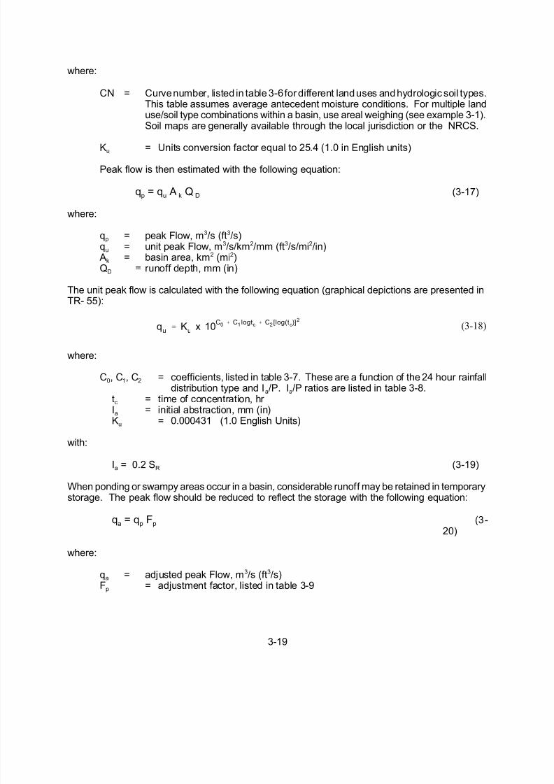
where:

CN = Curve number, listed in table 3-6 for different land uses and hydrologic soil types.This table assumes average antecedent moisture conditions. For multiple landuse/soil type combinations within a basin, use areal weighing (see example 3-1).Soil maps are generally available through the local jurisdiction or the NRCS.

Ku = Units conversion factor equal to 25.4 (1.0 in English units)

Peak flow is then estimated with the following equation:

qp = qu A k Q D (3-17)

where:

qp = peak Flow, m3/s (ft3/s)qu = unit peak Flow, m3/s/km2/mm (ft3/s/mi2/in)

Ak = basin area, km2 (mi2)Q

D

= runoff depth, mm (in)

The unit peak flow is calculated with the following equation (graphical depictions are presented inTR- 55):

where:

C0, C1, C2 = coefficients, listed in table 3-7. These are a function of the 24 hour rainfalldistribution type and Ia/P. Ia/P ratios are listed in table 3-8.

tc = time of concentration, hr

Ia = initial abstraction, mm (in)Ku = 0.000431 (1.0 English Units)

with:

Ia = 0.2 SR (3-19)

When ponding or swampy areas occur in a basin, considerable runoff may be retained in temporarystorage. The peak flow should be reduced to reflect the storage with the following equation:

qa = qp Fp (3-20)

where:

qa = adjusted peak Flow, m3/s (ft3/s)Fp = adjustment factor, listed in table 3-9



3-20

This method has a number of limitations which can have an impact on the accuracy of estimatedpeak flows:

C Basin should have fairly homogeneous CN valuesC CN should be 40 or greater C tc should be between 0.1 and 10 hr

C Ia/P should be between 0.1 and 0.5C Basin should have one main channel or branches with nearly equal times of concentrationC Neither channel nor reservoir routing can be incorporatedC Fp factor is applied only for ponds and swamps that are not in the t c Flow path

Example 3-5

Given: The following physical and hydrologic conditions.

• 3.3 sq km (1.27 mi 2 ) of fair condition open space and 2.8 sq km (1.08 mi 2 )of large lot residential • Negligible pond and swamp land • Hydrologic soil type C • Average antecedent moisture conditions• Time of concentration is 0.8 hr • 24-hour, type II rainfall distribution, 10-year rainfall of 150 mm (5.9 in)

Find: The 10-year peak flow using the SCS peak flow method.

Solution:

SI Units

Step 1: Calculate the composite curve number using table 3-6 and equation 3-2.

CN = 3 (CN x A x )/A = [3.3(79) + 2.8(77)]/(3.3 + 2.8) = 78

Step 2: Calculate the retention, SR , using equation 3-16.

SR = 25.4(1000/CN - 10) = 25.4 [(1000/78) - 10] = 72 mm

Step 3: Calculate the depth of direct runoff using equation 3-15.

QD = (P-0.2SR )2 / (P+0.8SR ) = [150 - 0.2(72)] 2 /[[150 + 0.8(72)] = 89 mm

Step 4: Determine I a /P from table 3-8.

I a /P = 0.10

Step 5: Determine coefficients from table 3-7.

C 0 = 2.55323 C 1 = -0.61512 C 2 = -0.16403



3-21

qu

(0.000431) (10C 0 C 1 log t c C 2 (log t c)

2

)

qu

(0.000431) (10[2.55323 (0.61512) log (0.8) (0.16403) [log (0.8)]2])

qu 0.176 m 3/ s/km 2/mm

qu

(1.0) (10C 0 C 1 log t c C 2 (log t c)

2

)

qu

(1.0) (10[2.55323 (0.61512) log (0.8) (0.16403) [log (0.8)]2])

Step 6: Calculate unit peak flow using equation 3-18.

Step 7: Calculate peak flow using equation 3-17.

q p = qu Ak QD = (0.176)(3.3 + 2.8)(89) = 96 m3 /s

English Units

Step 1: Calculate the composite curve number using table 3-6 and equation 3-2.

CN = 3 (CN x A x )/A = [1.27(79) + 1.08(77)]/(1.27 + 1.08) = 78

Step 2: Calculate the retention, SR , using equation 3-16.

SR = 1.0(1000/CN - 10) = 1.0[(1000/78) - 10] = 2.82 in

Step 3: Calculate the depth of direct runoff using equation 3-15.

QD = (P-0.2SR )2 / (P+0.8SR ) = [5.9 - 0.2(2.82)] 2 /[5.9 + 0.8(2.82)] = 3.49in

Step 4: Determine I a /P from equation I a = 0.2 SR .

I a = 0.2 (2.82) = 0.564

I a /P = 0.564/5.9 0.096 say 0.10

Step 5: Determine coefficients from table 3-7.

C 0 = 2.55323 C 1 = -0.61512 C 2 = -0.16403

Step 6: Calculate unit peak flow using equation 3-18.

qu = 409 ft 3 /s/mi 2 /in

Step 7: Calculate peak flow using equation 3-17.

q p = qu Ak QD = (409)(2.35)(3.49) = 3354 ft 3 /s



3-22

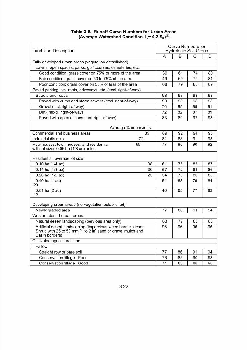
Table 3-6. Runoff Curve Numbers for Urban Areas(Average Watershed Condition, Ia= 0.2 SR)(6).

Land Use DescriptionCurve Numbers for

Hydrologic Soil Group

A B C D

Fully developed urban areas (vegetation established)Lawns, open spaces, parks, golf courses, cemeteries, etc.

Good condition; grass cover on 75% or more of the area 39 61 74 80

Fair condition; grass cover on 50 to 75% of the area 49 69 79 84

Poor condition; grass cover on 50% or less of the area 68 79 86 89

Paved parking lots, roofs, driveways, etc. (excl. right-of-way)

Streets and roads 98 98 98 98

Paved with curbs and storm sewers (excl. right-of-way) 98 98 98 98

Gravel (incl. right-of-way) 76 85 89 91

Dirt (inexcl. right-of-way) 72 82 87 89

Paved with open ditches (incl. right-of-way) 83 89 92 93

Average % impervious

Commercial and business areas 85 89 92 94 95

Industrial districts 72 81 88 91 93

Row houses, town houses, and residential 65with lot sizes 0.05 ha (1/8 ac) or less

77 85 90 92

Residential: average lot size

0.10 ha (1/4 ac) 38 61 75 83 87

0.14 ha (1/3 ac) 30 57 72 81 86

0.20 ha (1/2 ac) 25 54 70 80 85

0.40 ha (1 ac)

20

51 68 79 84

0.81 ha (2 ac)12

46 65 77 82

Developing urban areas (no vegetation established)

Newly graded area 77 86 91 94

Western desert urban areas:

Natural desert landscaping (pervious area only) 63 77 85 88

Artificial desert landscaping (impervious weed barrier, desertShrub with 25 to 50 mm [1 to 2 in] sand or gravel mulch andBasin borders)

96 96 96 96

Cultivated agricultural land

Fallow

Straight row or bare soil 77 86 91 94

Conservation tillage Poor 76 85 90 93

Conservation tillage Good 74 83 88 90



3-23

Table 3-7. Coefficients for SCS Peak Discharge Method (Equation 3-18)(6).

Rainfall Type Ia/P C0 C1 C2

I 0.10 2.30550 -0.51429 -0.11750

0.20 2.23537 -0.50387 -0.08929

0.25 2.18219 -0.48488 -0.06589

0.30 2.10624 -0.45695 -0.02835

0.35 2.00303 -0.40769 -0.01983

0.40 1.87733 -0.32274 0.05754

0.45 1.76312 -0.15644 0.00453

0.50 1.67889 -0.06930 0.0

IA 0.10 2.03250 -0.31583 -0.13748

0.20 1.91978 -0.28215 -0.070200.25 1.83842 -0.25543 -0.02597

0.30 1.72657 -0.19826 0.02633

0.50 1.63417 -0.09100 0.0

II 0.10 2.55323 -0.61512 -0.16403

0.30 2.46532 -0.62257 -0.11657

0.35 2.41896 -0.61594 -0.08820

0.40 2.36409 -0.59857 -0.05621

0.45 2.29238 -0.57005 -0.02281

0.50 2.20282 -0.51599 -0.01259

III 0.10 2.47317 -0.51848 -0.17083

0.30 2.39628 -0.51202 -0.13245

0.35 2.35477 -0.49735 -0.11985

0.40 2.30726 -0.46541 -0.11094

0.45 2.24876 -0.41314 -0.11508

0.50 2.17772 -0.36803 -0.09525



3-24

Table 3-8. Ia /P for Selected Rainfall Depths and Curve Numbers(6).Rainfall

mm (in)

Runoff Curve Number (CN)

40 45 50 55 60 65 70 75 80 85 90 95

10 0.39 * * * * * * * * * * * 0.27

20 0.79 * * * * * * * * * 0.45 0.28 0.13

30 1.18 * * * * * * * * 0.42 0.30 0.19 +40 1.57 * * * * * * * 0.42 0.32 0.22 0.14 +

50 1.97 * * * * * * 0.44 0.34 0.25 0.18 0.11 +

60 2.36 * * * * * 0.46 0.36 0.28 0.21 0.15 + +

70 2.76 * * * * 0.48 0.39 0.31 0.24 0.18 0.13 + +

80 3.15 * * * * 0.42 0.34 0.27 0.21 0.16 0.11 + +

90 3.54 * * * 0.46 0.38 0.30 0.24 0.19 0.14 0.10 + +

100 3.94 * * * 0.42 0.34 0.27 0.22 0.17 0.13 + + +

110 4.33 * * 0.46 0.38 0.31 0.25 0.20 0.15 0.12 + + +

120 4.72 * * 0.42 0.35 0.28 0.23 0.18 0.14 0.11 + + +

130 5.12 * 0.48 0.39 0.32 0.26 0.21 0.17 0.13 0.10 + + +

140 5.51 * 0.44 0.36 0.30 0.24 0.20 0.16 0.12 + + + +150 5.91 * 0.41 0.34 0.28 0.23 0.18 0.15 0.11 + + + +

160 6.30 0.48 0.39 0.32 0.26 0.21 0.17 0.14 0.11 + + + +

170 6.69 0.45 0.37 0.30 0.24 0.20 0.16 0.13 0.10 + + + +

180 7.09 0.42 0.34 0.28 0.23 0.19 0.15 0.12 + + + + +

190 7.48 0.40 0.33 0.27 0.22 0.18 0.14 0.11 + + + + +

200 7.87 0.38 0.31 0.25 0.21 0.17 0.14 0.11 + + + + +

210 8.27 0.36 0.30 0.24 0.20 0.16 0.13 0.10 + + + + +

220 8.66 0.35 0.28 0.23 0.19 0.15 0.12 0.10 + + + + +

230 9.06 0.33 0.27 0.22 0.18 0.15 0.12 + + + + + +

240 9.45 0.32 0.26 0.21 0.17 0.14 0.11 + + + + + +

250 9.84 0.30 0.25 0.20 0.17 0.14 0.11 + + + + + +

260 10.24 0.29 0.24 0.20 0.16 0.13 0.11 + + + + + +

270 10.63 0.28 0.23 0.19 0.15 0.13 0.10 + + + + + +

280 11.02 0.27 0.22 0.18 0.15 0.12 0.10 + + + + + +

290 11.42 0.26 0.21 0.18 0.14 0.12 + + + + + + +

300 11.81 0.25 0.21 0.17 0.14 0.11 + + + + + + +

310 12.20 0.25 0.20 0.16 0.13 0.11 + + + + + + +

320 12.60 0.24 0.19 0.16 0.13 0.11 + + + + + + +

330 12.99 0.23 0.19 0.15 0.13 0.10 + + + + + + +

340 13.39 0.22 0.18 0.15 0.12 0.10 + + + + + + +

350 13.78 0.22 0.18 0.15 0.12 0.10 + + + + + + +

360 14.17 0.21 0.17 0.14 0.12 + + + + + + + +

370 14.57 0.21 0.17 0.14 0.11 + + + + + + + +

380 14.96 0.20 0.16 0.13 0.11 + + + + + + + +

390 15.35 0.20 0.16 0.13 0.11 + + + + + + + +

400 15.75 0.19 0.16 0.13 0.10 + + + + + + + +

* signifies that Ia/P = 0.50 should be used + signifies that Ia/P = 0.10 should be used



3-25

Table 3-9. Adjustment Factor (Fp) for Pond and Swamp Areas that areSpread Throughout the Watershed.

Area of Pond or Swamp (%) Fp

0.0 1.00

0.2 0.971.0 0.87

3.0 0.75

5.0 0.72

3.3 Development of Design Hydrographs

This section discusses methods used to develop a design hydrograph. Hydrograph methods canbe computationally involved so computer programs such as HEC-1, TR-20, TR-55, and HYDRAINare almost exclusively used to generate runoff hydrographs. Hydrographic analysis is performedwhen flow routing is important such as in the design of stormwater detention, other water quality

facilities, and pump stations. They can also be used to evaluate flow routing through large stormdrainage systems to more precisely reflect flow peaking conditions in each segment of complexsystems. Reference 6 contains additional information on hydrographic methods.

3.3.1 Unit Hydrograph Methods

A unit hydrograph is defined as the direct runoff hydrograph resulting from a rainfall event that hasa specific temporal and spatial distribution and that lasts for a unit duration of time. The ordinatesof the unit hydrograph are such that the volume of direct runoff represented by the area under thehydrograph is equal to one millimeter of runoff from the drainage area(6). In the development of aunit hydrograph, there are several underlying assumptions made such as uniform rainfall intensity

and duration over the entire watershed. To minimize the effects of non-uniform intensity, a largestorm that encompasses the majority of the watershed should be employed. Additionally, stormmovement can effect the runoff characteristics of the watershed. Storms moving down a long andnarrow watersheds will produce a higher peak runoff rate and a longer time to peak. In order toovercome these limitations, unit hydrographs should be limited to drainage areas less than 2590km2 (1000 mi2)(6). Two synthetic unit hydrograph methods, Snyder’s and SCS’s, are discussed inthis chapter.

3.3.1.1 Snyder Synthetic Unit Hydrograph

This method, developed in 1938, has been used extensively by the Corps of Engineers andprovides a means of generating a synthetic unit hydrograph. In the Snyder method, empirically

defined terms and the physiographic characteristics of the drainage basin are used to determinea unit hydrograph. The key parameters which are explicitly calculated are the lag time, the unithydrograph duration, the peak discharge, and the hydrograph time widths of 50 percent and 75percent of the peak discharge. With these points, a characteristic unit hydrograph is sketched.The volume of this hydrograph is then checked to ensure it equals one millimeter of runoff. If itdoes not, it is adjusted accordingly. A typical Snyder hydrograph is shown in figure 3-6. In thefigure:



3-26

Figure 3-6. Snyder synthetic hydrograph definition.

TR = duration of unit excess rainfall, hr TL = lag time from the centroid of the unit rainfall excess to the

peakof the unit hydrograph, hr

tp = time to peak flow of hydrograph, hr W50, W75 = time width of unit hydrograph at discharge equal to 50 percent and

75percent, respectively, hr

tb = time duration of the unit hydrograph, hr

The Snyder Unit Hydrograph was developed for watersheds in the Appalachian highlands;however, the general method has been successfully applied throughout the country by appropriatemodification of empirical constants employed in the method (6). Additional information and anexample problem that describes the procedures for computing the Snyder Synthetic UnitHydrograph can be found in HDS 2(6).



3-27

3.3.1.2 SCS (NRCS) Tabular Hydrograph

The Soil Conservation Service (now known as the National Resources Conservation Service) hasdeveloped a tabular method which is used to estimate partial composite flood hydrographs at anypoint in a watershed. This method is generally applicable to small, nonhomogeneous areas whichmay be beyond the limitations of the Rational Method. It is applicable for estimating the effects of

land use change in a portion of the watershed as well as estimating the effects of proposedstructures(13).

The SCS Tabular Hydrograph method is based on a series of unit discharge hydrographsexpressed in cubic meters of discharge per second per square kilometer (cubic feet of dischargeper second per square mile) of watershed per millimeter (in) of runoff. A series of these unitdischarge hydrographs are provided in reference 13 for a range of subarea times of concentration(Tc) from 0.1 hr to 2 hours, and reach travel times (Tt) from 0 to 3 hours. Tables 3-10 and 3-11provides one such tabulation in SI and English units respectively.

The hydrograph ordinates for a specific time are determined by multiplying together the runoff depth, the subarea, and the tabular hydrograph unit discharge value for that time as determinedfrom the tables. See equation 3-21:

q = qt A QD (3-21)

where:

q = hydrograph ordinate for a specific time, m3/s (ft3/s)qt = tabular hydrograph unit discharge from appropriate table,

m3/s/km2/mm (ft3/s/mi2/in) A = sub-basin drainage area, km2 (mi2)QD = runoff depth, mm (in)

Chapter 5 of reference 13 provides a detailed description of the tabular hydrograph method. Indeveloping the tabular hydrograph, the watershed is divided into homogeneous subareas. Inputparameters required for the procedure include, (1) the 24-hour rainfall amount, mm (in), (2) anappropriate rainfall distribution (I, IA, II, or III), (3) the runoff curve number, CN, (4) the time of concentration, Tc, (5) the travel time, Tt, and (6) the drainage area, km2 (mi2) for each subarea. The24-hour rainfall amount, rainfall distribution, and the runoff curve number are used in equations 3-15 and 3-16 to determine the runoff depth in each subarea. The product of the runoff depth timesdrainage is multiplied times each tabular hydrograph value to determine the final hydrographordinate for a particular subarea. Subarea hydrographs are then added to determine the finalhydrograph at a particular point in the watershed. Example 3-6 provides an illustration of the useof the tabular hydrograph method.

Assumptions and limitations inherent in the tabular method are as follows:

• Total area should be less than 800 hectares (2000 acres). Typically, subareas are far smaller than this because the subareas should have fairly homogeneous land use.

• Travel time is less than or equal to 3 hours.• Time of concentration is less than or equal to 2 hours.• Drainage areas of individual subareas differ by less than a factor of five.



3-28

Example 3-6

Given: A watershed with three subareas. Subareas 1 and 2 both drain into subarea 3.Basin data for the three subareas are as follows:

Area (km2 ) (mi 2 ) t c (hr) T t (hr) CN

Subarea 1Subarea 2 Subarea 3

1.0 0.386 0.5 0.1932.4 0.927

0.5 0.5 0.5

------

0.20

75 65 70

A time of concentration, t c , of 0.5 hr, an IA/P value of 0.10, and a type II storm distribution areassumed for convenience in all three subareas. The travel time applies to the reach for thecorresponding area; therefore, the travel time in subarea 3 will apply to the tabular hydrographsrouted from subareas 1 and 2.

Find : The outlet hydrograph for a 150-mm (5.9 in) storm.

Solution:SI Units

Step 1: Calculate the retention for each of the subareas using equation (3-16).

SR = Ku (1000/CN - 10) with Ku = 25.4

Subarea 1. SR = 25.4 (1000/75 - 10) = 85 mmSubarea 2. SR = 25.4 (1000/65 - 10) = 137 mmSubarea 3. SR = 25.4 (1000/70 - 10) = 109 mm

Step 2: Calculate the depth of runoff for each of the subareas using equation (3-15).

QD = [P - 0.2 (SR )] 2

/ [P + 0.8 (SR )]

Subarea 1. QD = [150 - 0.2 (85)] 2 /[150 + 0.8 (85)] = 81 mmSubarea 2. QD = [150 - 0.2 (137)] 2 /[150 + 0.8 (137)] = 58 mmSubarea 3. QD = [150 - 0.2 (109)] 2 /[150 + 0.8 (109)] = 69 mm

Step 3: Calculate ordinate values using Equation 3-21 q = qt A Q

Multiply the appropriate tabular hydrograph values (qt ) from table 3-10 (SI Units) by thesubarea areas (A) and runoff depths (Q) and sum the values for each time to give thecomposite hydrograph at the end of subarea 3. For example, the hydrograph flow contributed from subarea 1 (t c = 0.5 hr, T t = 0.20 hr) at 12.0 hr is calculated as the product of the tabular value, the area, and the runoff depth, or 0.020 (1.0)(81) = 1.6 m 3 /s.

The following table lists the subarea and composite hydrographs. Please note that thisexample does not use every hydrograph time ordinate.



3-29

Flow at specified time (m3 /s)

11(hr)

12 (hr)

12.2 (hr)

12.4(hr)

12.5 (hr)

12.6 (hr)

12.8 (hr)

13(hr)

14(hr)

16 (hr)

20 (hr)

Subarea 1Subarea 2

Subarea 3

0.5 0.2

1.2

1.6 0.6

6.8

4.11.5

22.0

11.6 4.1

37.8

15.15.4

36.3

16.7 6.0

28.6

13.2 4.7

16.1

8.33.0

10.0

1.90.7

3.3

1.0 0.3

1.8

0.5 0.2

1.0 Total 1.9 9.0 27.6 53.5 56.8 51.3 34.0 21.3 5.9 3.1 1.7

English Units

Step 1: Calculate the retention for each of the subareas using equation (3-16).

SR = Ku (1000/CN - 10) with Ku =1.0

Subarea 1. SR = 1.0 (1000/75 - 10) = 3.33 inSubarea 2. SR = 1.0 (1000/65 - 10) = 5.38 in

Subarea 3. SR = 1.0 (1000/70 - 10) = 4.29 in

Step 2: Calculate the depth of runoff for each of the subareas using equation (3-15).

QD = [P - 0.2 (SR )] 2 / [P + 0.8 (SR )]

Subarea 1. QD = [5.9 - 0.2 (85)] 2 /[5.9 + 0.8 (85)] = 3.2 inSubarea 2. QD = [5.9 - 0.2 (137)] 2 /[5.9 + 0.8 (137)] = 2.28 inSubarea 3. QD = [5.9 - 0.2 (109)] 2 /[5.9 + 0.8 (109)] = 2.72 in

Step 3: Multiply the appropriate tabular hydrograph values from table 3-10 (English Units) by thesubarea areas and runoff depths and sum the values for each time to give the compositehydrograph at the end of subarea 3. For example, the hydrograph flow contributed from

subarea 1 (t c = 0.5 hr, T t = 0.20 hr) at 12.0 hr is calculated as the product of the tabular value, the area, and the runoff depth, or 47 (0.386) 3.2 = 58 ft 3 /s

The following table lists the subarea and composite hydrographs. Please note that thisexample does not use every hydrograph time ordinate.

Flow at specified time (ft 3 /s)

11(hr)

12 (hr)

12.2 (hr)

12.4(hr)

12.5 (hr)

12.6 (hr)

12.8 (hr)

13(hr)

14(hr)

16 (hr)

20 (hr)

Subarea 1Subarea 2

Subarea 3

17 6

43

58 21

238

14351

778

410 146

1337

536 191

1281

584210

1016

466 166

571

294105

354

65 23

119

3312

66

17 6

35

Total 66 317 972 1893 2008 1815 1203 753 207 111 58



3-30



3-31



3-32

qp Ku Ak QD

tp

(3-22)

tp

2

3tc (3-23)

qp Ku Ak QD

tc

(3-24)

3.3.1.3 SCS (NRCS) Synthetic Unit Hydrograph

The Soil Conservation Service (now known as the Natural Resources Conservation Service) hasdeveloped a synthetic unit hydrograph procedure that has been widely used in their conservationand flood control work. The unit hydrograph used by this method is based upon an analysis of alarge number of natural unit hydrographs from a broad cross section of geographic locations and

hydrologic regions. This method is easy to apply. The only parameters that need to be determinedare the peak discharge and the time to peak. A standard unit hydrograph is constructed usingthese two parameters.

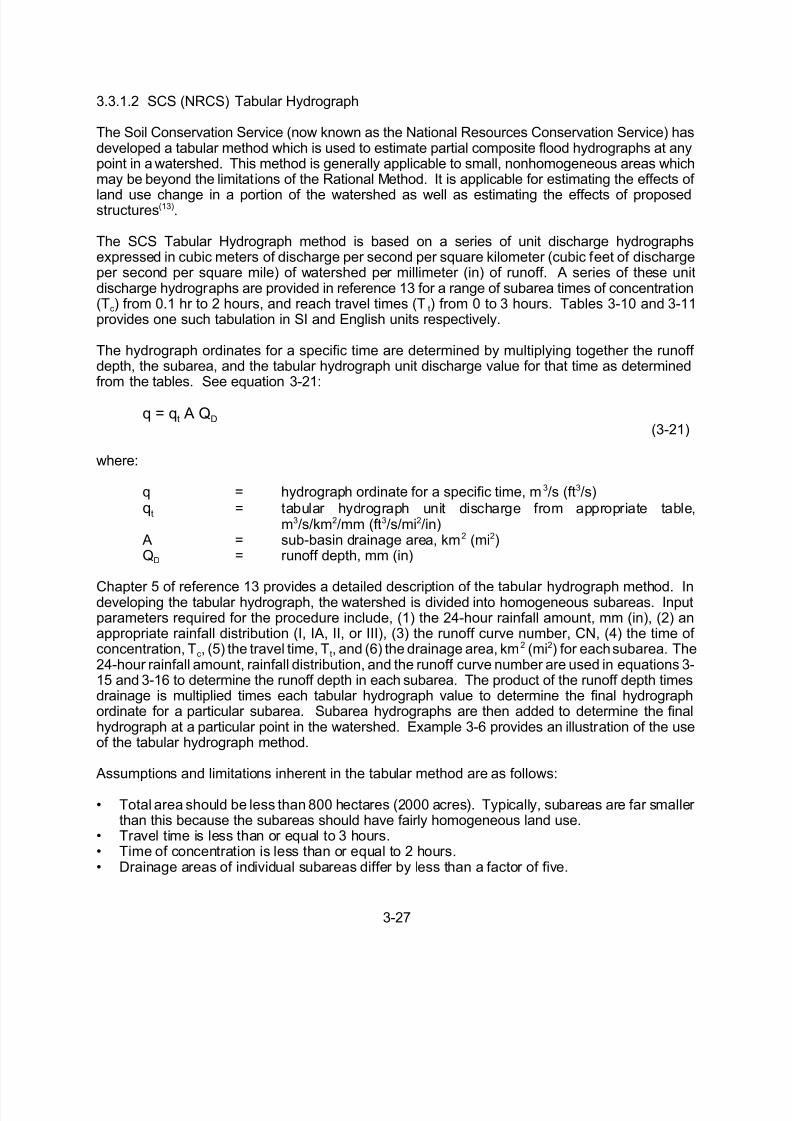
For the development of the SCS Unit Hydrograph, the curvilinear unit hydrograph is approximatedby a triangular unit hydrograph (UH) that has similar characteristics. Figure 3-7 shows acomparison of the two dimensionless unit hydrographs. Even though the time base of thetriangular UH is 8/3 of the time to peak and the time base of the curvilinear UH is five times thetime to peak, the area under the two UH types is the same.

The area under a hydrograph equals the volume of direct runoff QD which is one millimeter or oneinch for a unit hydrograph. The peak flow is calculated as follows:

where:

qp = peak Flow, m3/s (ft3/s) Ak = drainage area, km2 (mi2)QD = volume of direct runoff ( = 1 for unit hydrograph), mm (in)tp = time to peak, hr Ku = 2.083 (483.5 in English units)

The constant 2.083 reflects a unit hydrograph that has 3/8 of its area under the rising limb. For mountainous watersheds, the fraction could be expected to be greater than 3/8, and therefore theconstant may be near 2.6. For flat, swampy areas, the constant may be on the order of 1.3.

Appropriate changes in the English unit constant should also be made.

Time to peak, tp, can be expressed in terms of time of concentration, tc, as follows:

Expressing qp in terms of tc rather than tp yields:

where Ku = 3.125 (725.25 For English units)



3-33

q p

K c

Ak

QD

t c

3.125 (1.2) (1)

1.34 2.8 m 3/ s

q p

K u

Ak

QD

t c q p

K u

Ak

QD

t c

725.25 (0.463) (1.0)

1.34 250.59 ft 3/ s

Figure 3-7. Dimensionless curvilinear SCS synthetic unit hydrograph and equivalenttriangular hydrograph.

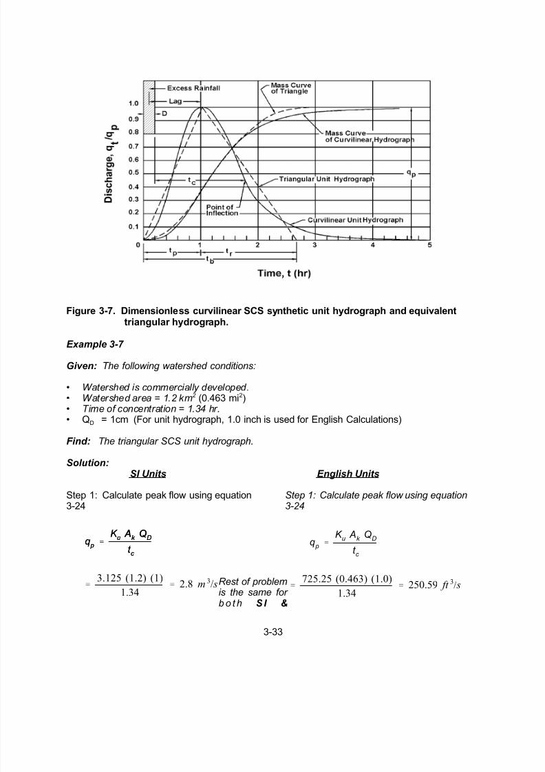
Example 3-7

Given: The following watershed conditions:

• Watershed is commercially developed.• Watershed area = 1.2 km2 (0.463 mi2)

• Time of concentration = 1.34 hr.• QD = 1cm (For unit hydrograph, 1.0 inch is used for English Calculations)

Find: The triangular SCS unit hydrograph.

Solution:SI Units

Step 1: Calculate peak flow using equation3-24

English Units

Step 1: Calculate peak flow using equation3-24

Rest of problemis the same for b o t h S I &



3-34

t p

2

3

t c

2

3

(1.34) 0.893 hr

t b

8

3(0.893) 2.38 hr

Figure 3-8. Example: The triangular unit hydrograph.

English Units

Step 2: Calculate time to peak using equation 3-23.

Step 3: Calculate time base of UH.Step 4: Draw resulting triangular UH (see figure 3-8).

Note: The curvilinear SCS UH is more commonly used and is incorporated into many computer

programs .



3-35

TL

KL

L0.62

M

SL 0.31 (13BDF)0.47 (3-25)

Table 3-11. USGS Dimensionless Hydrograph Coordinates.

Abscissa Ordinate Abscissa Ordinate

0.0 0.00 1.3 0.65

0.1 0.04 1.4 0.54

0.2 0.08 1.5 0.44

0.3 0.14 1.6 0.36

0.4 0.21 1.7 0.30

0.5 0.37 1.8 0.25

0.6 0.56 1.9 0.21

0.7 0.76 2.0 0.17

0.8 0.92 2.1 0.13

0.9 1.00 2.2 0.10

1.0 0.98 2.3 0.06

1.1 0.90 2.4 0.03

1.2 0.78 2.5 0.00

3.3.2 USGS Nationwide Urban Hydrograph

The USGS nationwide urban hydrograph method uses information developed by the USGS thatapproximates the shape and characteristics of hydrographs. Information required for using thismethod are: (1) dimensionless hydrograph ordinates; (2) time lag; and (3) peak flow. Table 3-11lists default values for the dimensionless hydrograph ordinates derived from the nationwide urbanhydrograph study. These values provide the shape of the dimensionless hydrograph(17).

Time lag is computed using the following relationship:

where:

TL = time lag, hr KL = 0.38 (0.85 in English units)LM = main channel length, km (mi)SL = main channel slope, m/km (ft/mi)BDF = basin development factor (see discussion in section 3.2.3)

The peak flow can be computed using one of the methods described in section 3-2. Applicationof this method proceeds by first multiplying the abscissae in table 3-11 by the time lag between thecentroid of the rainfall and the centroid of the runoff computed using equation 3-25. Then the

ordinates in table 3-11. are multiplied by the peak flow computed using an appropriate method.The resultant is the design hydrograph. The following example illustrates the design of ahydrograph using the USGS nationwide urban hydrograph method.

Example 3-8



3-36

TL KL L0.62

M SL 0.31 (13 BDF)0.47

0.38 (1.1)0.62 (3.6)0.31 (130)0.47

0.9hr

TL KL L0.62

M SL 0.31 (13 BDF)0.47

0.38 (0.9)0.62 (4.2)0.31 (136)0.47

0.57hr

TL KL L0.62

M SL 0.31 (13 BDF)0.47

0.85 (0.68)0.62 (19)0.31 (130)0.47

0.9hr

TL KL L0.62

M SL 0.31 (13 BDF)0.47

0.85 (0.56)0.62 (22)0.31 (136)0.47

0.57hr

Given: Site data from example 3-3 and supplementary data as follows:

Existing conditions (unimproved)

• 10 - year peak flow = 0.55 m3 /s (19.4 ft 3 /s)• LM = 1.1 km (0.68 mi)

• SL = 3.6 m/km (19 ft/mi)• BDF = 0

Proposed conditions (improved)

• 10 - year peak flow = 0.88 m3 /s (31.2 ft 3 /s)• LM = 0.9 km (0.56 mi)• SL = 4.2 m/km (22 ft/mi)• BDF = 6

Find: The ordinates of the USGS nationwide urban hydrograph as applied to the site.

Solution:

SI Units

Step 1: Calculate time lag with equation3-25

Existing conditions (unimproved )

Proposed conditions (improved)

English Units

Step 1: Calculate time lag with equation 3-25.

Existing conditions (unimproved):

Pr o

posed conditions (improved)

Step 2: Multiply lag time by abscissa and peak flow by ordinate in table 3-11 to form hydrographcoordinates as illustrated in the following tables:



3-37

SI Units

USGS Nationwide Urban Hydrograph for existing conditions (unimproved):

Time (hr) Flow (m3 /s) Time (hr) Flow (m3 /s)

(0.0)(0.89) = 0.00 (0.1)(0.89) = 0.09(0.2)(0.89) = 0.18 (0.3)(0.89) = 0.27 (0.4)(0.89) = 0.36 (0.5)(0.89) = 0.45 (0.6)(0.89) = 0.53(0.7)(0.89) = 0.62 (0.8)(0.89) = 0.71(0.9)(0.89) = 0.80 (1.0)(0.89) = 0.89

(1.1)(0.89) = 0.98 (1.2)(0.89) = 1.07

(0.00)(0.55) = 0.00 (0.04)(0.55) = 0.02 (0.08)(0.55) = 0.04(0.14)(0.55) = 0.08 (0.21)(0.55) = 0.12 (0.37)(0.55) = 0.20 (0.56)(0.55) = 0.31(0.76)(0.55) = 0.42 (0.92)(0.55) = 0.51(1.00)(0.55) = 0.55 (0.98)(0.55) = 0.54

(0.90)(0.55) = 0.50 (0.78)(0.55) = 0.43

(1.3)(0.89) = 1.16 (1.4)(0.89) = 1.25 (1.5)(0.89) = 1.34(1.6)(0.89) = 1.42 (1.7)(0.89) = 1.51(1.8)(0.89) = 1.60 (1.9)(0.89) = 1.69(2.0)(0.89) = 1.78 (2.1)(0.89) = 1.87 (2.2)(0.89) = 1.96 (2.3)(0.89) = 2.05

(2.4)(0.89) = 2.14(2.5)(0.89) = 2.23

(0.65)(0.55) = 0.36 (0.54)(0.55) = 0.30 (0.44)(0.55) = 0.24(0.36)(0.55) = 0.20 (0.30)(0.55) = 0.17 (0.25)(0.55) = 0.14(0.21)(0.55) = 0.12 (0.17)(0.55) = 0.09(0.13)(0.55) = 0.07 (0.10)(0.55) = 0.06 (0.06)(0.55) = 0.03

(0.03)(0.55) = 0.02 (0.00)(0.55) = 0.00

USGS Nationwide Urban Hydrograph for proposed conditions (improved):

Time (hr) Flow (m3 /s) Time (hr) Flow (m3 /s)

(0.0)(0.57) = 0.00 (0.1)(0.57) = 0.06 (0.2)(0.57) = 0.11

(0.3)(0.57) = 0.17 (0.4)(0.57) = 0.23(0.5)(0.57) = 0.29(0.6)(0.57) = 0.34(0.7)(0.57) = 0.40 (0.8)(0.57) = 0.46 (0.9)(0.57) = 0.51(1.0)(0.57) = 0.57 (1.1)(0.57) = 0.63(1.2)(0.57) = 0.68

(0.00)(0.88) = 0.00 (0.04)(0.88) = 0.04(0.08)(0.88) = 0.07

(0.14)(0.88) = 0.12 (0.21)(0.88) = 0.18 (0.37)(0.88) = 0.33(0.56)(0.88) = 0.49(0.76)(0.88) = 0.67 (0.92)(0.88) = 0.81(1.00)(0.88) = 0.88 (0.98)(0.88) = 0.86 (0.90)(0.88) = 0.79(0.78)(0.88) = 0.69

(1.3)(0.57) = 0.74(1.4)(0.57) = 0.80 (1.5)(0.57) = 0.86

(1.6)(0.57) = 0.91(1.7)(0.57) = 0.97 (1.8)(0.57) = 1.03(1.9)(0.57) = 1.08 (2.0)(0.57) = 1.14(2.1)(0.57) = 1.20 (2.2)(0.57) = 1.25 (2.3)(0.57) = 1.31(2.4)(0.57) = 1.37 (2.5)(0.57) = 1.43

(0.65)(0.88) = 0.57 (0.54)(0.88) = 0.48 (0.44)(0.88) = 0.39

(0.36)(0.88) = 0.32 (0.30)(0.88) = 0.26 (0.25)(0.88) = 0.22 (0.21)(0.88) = 0.18 (0.17)(0.88) = 0.15 (0.13)(0.88) = 0.11(0.10)(0.88) = 0.09(0.06)(0.88) = 0.05 (0.03)(0.88) = 0.03(0.00)(0.88) = 0.00

The final hydrographs are shown in figure 3-9.



3-38

English Units

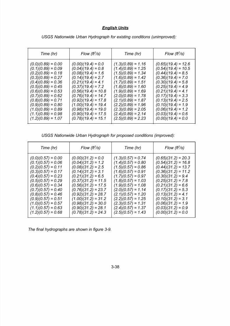
USGS Nationwide Urban Hydrograph for existing conditions (unimproved):

Time (hr) Flow (ft 3 /s) Time (hr) Flow (ft 3 /s)

(0.0)(0.89) = 0.00 (0.1)(0.89) = 0.09(0.2)(0.89) = 0.18 (0.3)(0.89) = 0.27 (0.4)(0.89) = 0.36 (0.5)(0.89) = 0.45 (0.6)(0.89) = 0.53(0.7)(0.89) = 0.62 (0.8)(0.89) = 0.71(0.9)(0.89) = 0.80 (1.0)(0.89) = 0.89

(1.1)(0.89) = 0.98 (1.2)(0.89) = 1.07

(0.00)(19.4) = 0.0 (0.04)(19.4) = 0.8 (0.08)(19.4) = 1.6 (0.14)(19.4) = 2.7 (0.21)(19.4) = 4.1(0.37)(19.4) = 7.2 (0.56)(19.4) = 10.8 (0.76)(19.4) = 14.7 (0.92)(19.4) = 17.8 (1.00)(19.4) = 19.4(0.98)(19.4) = 19.0

(0.90)(19.4) = 17.5 (0.78)(19.4) = 15.1

(1.3)(0.89) = 1.16 (1.4)(0.89) = 1.25 (1.5)(0.89) = 1.34(1.6)(0.89) = 1.42 (1.7)(0.89) = 1.51(1.8)(0.89) = 1.60 (1.9)(0.89) = 1.69(2.0)(0.89) = 1.78 (2.1)(0.89) = 1.87 (2.2)(0.89) = 1.96 (2.3)(0.89) = 2.05

(2.4)(0.89) = 2.14(2.5)(0.89) = 2.23

(0.65)(19.4) = 12.6 (0.54)(19.4) = 10.5 (0.44)(19.4) = 8.5 (0.36)(19.4) = 7.0 (0.30)(19.4) = 5.8 (0.25)(19.4) = 4.9(0.21)(19.4) = 4.1(0.17)(19.4) = 3.3(0.13)(19.4) = 2.5 (0.10)(19.4) = 1.9(0.06)(19.4) = 1.2

(0.03)(19.4) = 0.6 (0.00)(19.4) = 0.0

USGS Nationwide Urban Hydrograph for proposed conditions (improved):

Time (hr) Flow (ft 3 /s) Time (hr) Flow (ft 3 /s)

(0.0)(0.57) = 0.00 (0.1)(0.57) = 0.06 (0.2)(0.57) = 0.11

(0.3)(0.57) = 0.17 (0.4)(0.57) = 0.23(0.5)(0.57) = 0.29(0.6)(0.57) = 0.34(0.7)(0.57) = 0.40 (0.8)(0.57) = 0.46 (0.9)(0.57) = 0.51(1.0)(0.57) = 0.57 (1.1)(0.57) = 0.63(1.2)(0.57) = 0.68

(0.00)(31.2) = 0.0 (0.04)(31.2) = 1.2 (0.08)(31.2) = 2.5

(0.14)(31.2) = 3.1(0.21)(31.2) = 6.5 (0.37)(31.2) = 11.5 (0.56)(31.2) = 17.5 (0.76)(31.2) = 23.7 (0.92)(31.2) = 28.7 (1.00)(31.2) = 31.2 (0.98)(31.2) = 30.0 (0.90)(31.2) = 28.1(0.78)(31.2) = 24.3

(1.3)(0.57) = 0.74(1.4)(0.57) = 0.80 (1.5)(0.57) = 0.86

(1.6)(0.57) = 0.91(1.7)(0.57) = 0.97 (1.8)(0.57) = 1.03(1.9)(0.57) = 1.08 (2.0)(0.57) = 1.14(2.1)(0.57) = 1.20 (2.2)(0.57) = 1.25 (2.3)(0.57) = 1.31(2.4)(0.57) = 1.37 (2.5)(0.57) = 1.43

(0.65)(31.2) = 20.3(0.54)(31.2) = 16.8 (0.44)(31.2) = 13.7

(0.36)(31.2) = 11.2 (0.30)(31.2) = 9.4(0.25)(31.2) = 7.8 (0.21)(31.2) = 6.6 (0.17)(31.2) = 5.3(0.13)(31.2) = 4.1(0.10)(31.2) = 3.1(0.06)(31.2) = 1.9(0.03)(31.2) = 0.9(0.00)(31.2) = 0.0

The final hydrographs are shown in figure 3-9.



Figure 3-9. USGS Nationwide Urban Hydrograph for existing (unimproved) andproposed (improved) conditions.

Documents

Urban Hydrology