User Guide toThe Computational Morphometry Toolkit1

Release 1.20

Torsten Rohlfing

March 23, 2011

Neuroscience Program, SRI International, Menlo Park, CA2

Abstract

This guide is intended as a very brief introduction of the main tools in the Computational Mor-phometry Toolkit (CMTK), which is available in source code and as pre-compiled binaries fromhttp://www.nitrc.org/projects/cmtk/. The target audience of this document are CMTK users, who mightuse this document as a reference to the most common processing tasks, and prospective users, who mayfind this information useful to determine whether CMTK provides functionality that they can use. Wefocus in particular on a simplified workflow for deformation morphometry studies based on magneticresonance images: DICOM conversion, artifact correction, affine and nonlinear image registration, re-formatting, Jacobian determinant map generation, and statistical hypothesis testing.

1This document is licensed under the Creative Commons Attribution License Version 3.0.2Continued development and maintenance of CMTK is funded by the National Institute of Biomedical Imaging and Bioengi-

neering under Grant No. R01 EB008381.

Contents 2

Contents

1 Introduction 31.1 Coordinate Conventions . . . . . . . . . . . . . . . . . . . . . . . . . . . . . . . . . . . . . 31.2 Registration Terminology . . . . . . . . . . . . . . . . . . . . . . . . . . . . . . . . . . . . 51.3 Supported Image File Formats . . . . . . . . . . . . . . . . . . . . . . . . . . . . . . . . . 51.4 Toolkit-Global Command Line Options . . . . . . . . . . . . . . . . . . . . . . . . . . . . 6

2 Step-by-Step Morphometry 72.1 DICOM Image Stacker . . . . . . . . . . . . . . . . . . . . . . . . . . . . . . . . . . . . . 72.2 Interleaved Image Motion Artifact Correction . . . . . . . . . . . . . . . . . . . . . . . . . 82.3 MR Intensity Bias Field Correction . . . . . . . . . . . . . . . . . . . . . . . . . . . . . . . 82.4 Affine Image Registration . . . . . . . . . . . . . . . . . . . . . . . . . . . . . . . . . . . . 82.5 Nonrigid Image Registration . . . . . . . . . . . . . . . . . . . . . . . . . . . . . . . . . . 112.6 Reformating Registered Images . . . . . . . . . . . . . . . . . . . . . . . . . . . . . . . . 122.7 Jacobian Determinant Maps . . . . . . . . . . . . . . . . . . . . . . . . . . . . . . . . . . 132.8 Statistical Testing . . . . . . . . . . . . . . . . . . . . . . . . . . . . . . . . . . . . . . . . 132.9 Atlas-based Segmentation . . . . . . . . . . . . . . . . . . . . . . . . . . . . . . . . . . . 14

3 Atlas Construction 163.1 Averaging Pairwise Correspondences . . . . . . . . . . . . . . . . . . . . . . . . . . . . . . 163.2 Iterative Shape Averaging . . . . . . . . . . . . . . . . . . . . . . . . . . . . . . . . . . . . 163.3 Groupwise Population Registration . . . . . . . . . . . . . . . . . . . . . . . . . . . . . . . 16

4 More Gory Details 184.1 Registration Options for Image Pre-Processing . . . . . . . . . . . . . . . . . . . . . . . . 184.2 GPU-Accelerated Tools . . . . . . . . . . . . . . . . . . . . . . . . . . . . . . . . . . . . . 18

Index 22

3

1 Introduction

The Computational Morphometry Toolkit, or short CMTK, is a set of software tools that perform vari-ous types of processing and analysis on three-dimensional (3D) image data. CMTK is available both insource code (licensed under the GNU GPL3) and as pre-compiled binaries from http://www.nitrc.org/projects/cmtk/ .

CMTK is primarily a collection of command line tools, which make the toolkit ideally suited for unattendedbatch processing of large amounts of data. In addition, CMTK’s back-end libraries, which are shared by allcommand line tools, can be used as a relatively lightweight, yet powerful, platform for implementation ofnew image processing algorithms.

LATEX source for this User Guide, including all figures, can be checked out from the CMTK Subversionrepository via

svn co https://nitrc.org/svn/cmtk/trunk/doc/UserGuideCMTK/

1.1 Coordinate Conventions

For medical image data, CMTK uses an anatomy-based coordinate system, which we refer to as “RAS” coor-dinates. This means that the x direction of the coordinate space increases towards the anatomical “Right,” they direction increases towards the anatomical “Anterior,” and the z direction increases towards the anatomical“Superior.” The coordinate space origin, (0,0,0), thus coincides with the “Left-Posterior-Inferior” corner ofthe image volume.

All images that are read into one of CMTK’s tools are first reoriented to fit this coordinate system. Thismeans that the storage order of image pixels in memory is such that the fastest-varying of the three pixelindexes corresponds to the “Left”–”Right” anatomical direction, the second fastest to the “Posterior”–”Anterior” direction, and the slowest varying to the “Inferior”–”Superior” direction. Consequently, thefirst pixel in memory is the one that is the Left-Posterior-Inferior-most pixel anatomically.

For image file formats that define subject orientation based on direction vectors within an anatomy-basedcoordinate space, which is the majority of modern formats, CMTK determines the nearest anatomical ori-entation of the image within ±45 degrees around each rotation axis.

As a matter of policy, all of CMTK’s tools that write an output image file based on some input image filecan be expected to write the output image in the same pixel order and orientation as the input, so long as theoutput file format supports this. An example where this is not the case is when a file is read in NIFTI formatwith RAS pixel order, but written in Analyze 7.5 format, which does not support RAS order. In this case,the output would be written in LAS order as the closest matching orientation.

To confirm that images are read and written correctly, and to diagnose problems related to image orientation,CMTK comes with a very simple triplanar image viewer (see screen shot in Fig. 1), adequately named“triplanar .” The coordinates shown in this viewer for any image are exactly the coordinates that allCMTK tools use. Note that for the triplanar viewer to be available, CMTK must be built with support forthe Qt toolkit1 (version 4.3.0 or higher), and the “BUILD_GUI ” build option must be enabled.

1http://qt.nokia.com

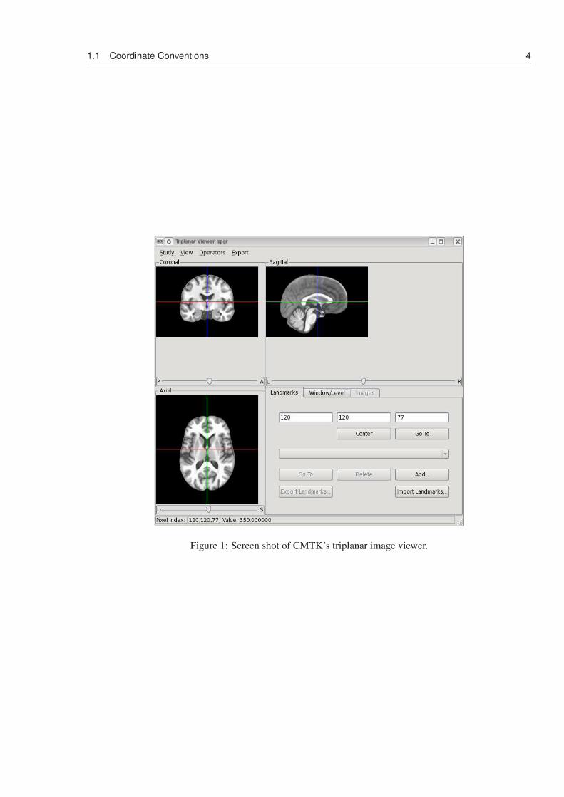
1.1 Coordinate Conventions 4

Figure 1: Screen shot of CMTK’s triplanar image viewer.

1.2 Registration Terminology 5

1.2 Registration Terminology

Since one of the primary strengths of CMTK is its selection of powerful and well-tested registration tools,we shall first clarify some important registration terminology. In pairwise registration, throughout this guideas well as in all tools and source code, we shall refer to one image as the reference and the other as thefloating image. Others may refer to these as the fixed and the moving image, respectively. By definition,all coordinate transformations computed by CMTK are functions that map from the space of the reference(fixed) image to the space of the floating (moving) image. As a result, when reformatting one image tomatch the other, it is the floating image by default that will be transformed to match the reference image.

Note that when we speak about transforming coordinates of features, such as landmarks or the nodes in amesh, then the coordinates of the reference image will be transformed to match the floating image.

1.3 Supported Image File Formats

CMTK supports a wide range of image file formats, both for import and export. When reading an image fileinto CMTK, its type is detected automatically. Note that in order to correctly identify the format of imageswith separate header and data files, it is necessary to provide CMTK with the path to the header file, not thedata file.

Whether a particular file can be read into CMTK can easily be tested using CMTK’s describe tool.For example, to test (and describe) the content of an Analyze 7.52 header/image pair, example.hdr andexample.img , one would run the following command:

describe example.hdr

When writing files, CMTK determines the desired file format based on the suffix of the output path. Thefollowing suffixes are supported:

nii Single-file NIfTI-1 image3.

img NIfTI image with detached header. Header file will be written with suffix .hdr

nrrd Single-file Nrrd4.

nhdr Nrrd with detached header. The data file will be written with .raw suffix.

hdr Analyze 7.5 detached header. The data file will be written with suffix img .

Note that both Analyze and NIfTI header/data file pairs use the suffixes .hdr and .img . For historic reasons,using .hdr as the output file suffix will always invoke Analyze export, whereas the .img suffix will invokeNIfTI export. Both formats need to be read using the .hdr file, however.

Note also that, by default, all data files are written with gzip compression. Because CMTK contains abundled zlib library, this is true even when the gzip tool itself is not installed. This behavior can bedisabled by defining the CMTK_WRITE_UNCOMPRESSED environment variable. On a Unix/Linux system usingthe csh shell, this would be achieved via

2http://eeg.sourceforge.net/ANALYZE75.pdf3http://nifti.nimh.nih.gov/nifti-1/4http://teem.sourceforge.net/nrrd/

1.4 Toolkit-Global Command Line Options 6

Option Function--help Write a summary of the tool command line options to standard

output.--wiki Write the command line option summary in MediaWiki markup

(this is convenient for creating a web-based command line de-scription collection.

--version Write the CMTK version to standard output.--verbose-level <n> Level of verbosity, where “<n> ” is an integer number from 0 to 9.

Default is 0 for essentially quiet operation. Higher levels producemore detailed status output for debugging.

--echo Write a copy of the entire command line to standard output. Thisis useful for debugging scripts, i.e., when it is unclear whether thetool is really invoked with the intended options and arguments.

--threads <n> Set maximum number of parallel threads to “<n> ” for the POSIXThreads and OpenMP parallelization models. This does not affectthe number of parallel jobs when using Grand Central Dispatchon MacOS-X, which determines the number of parallel tasks atsystem level.

Table 1: Command line options supported by all CMTK command line tools.

export CMTK_WRITE_UNCOMPRESSED=1

where only the definition of the variable is relevant, and its value is ignored. Thus, to re-enable compressedwriting, rather than setting the variable to “0” for example, use

unset CMTK_WRITE_UNCOMPRESSED

or its appropriate equivalent inside your favorite shell.

1.4 Toolkit-Global Command Line Options

All command line tools in CMTK support a set of options that control the global behaviour of the toolkit.These are summarized in Table 1. In addition, a number of tools also supports the “--xml ” option, whichprints a command line description in XML format for use of the tools as plugins in 3D Slicer5.

5http://www.slicer.org

7

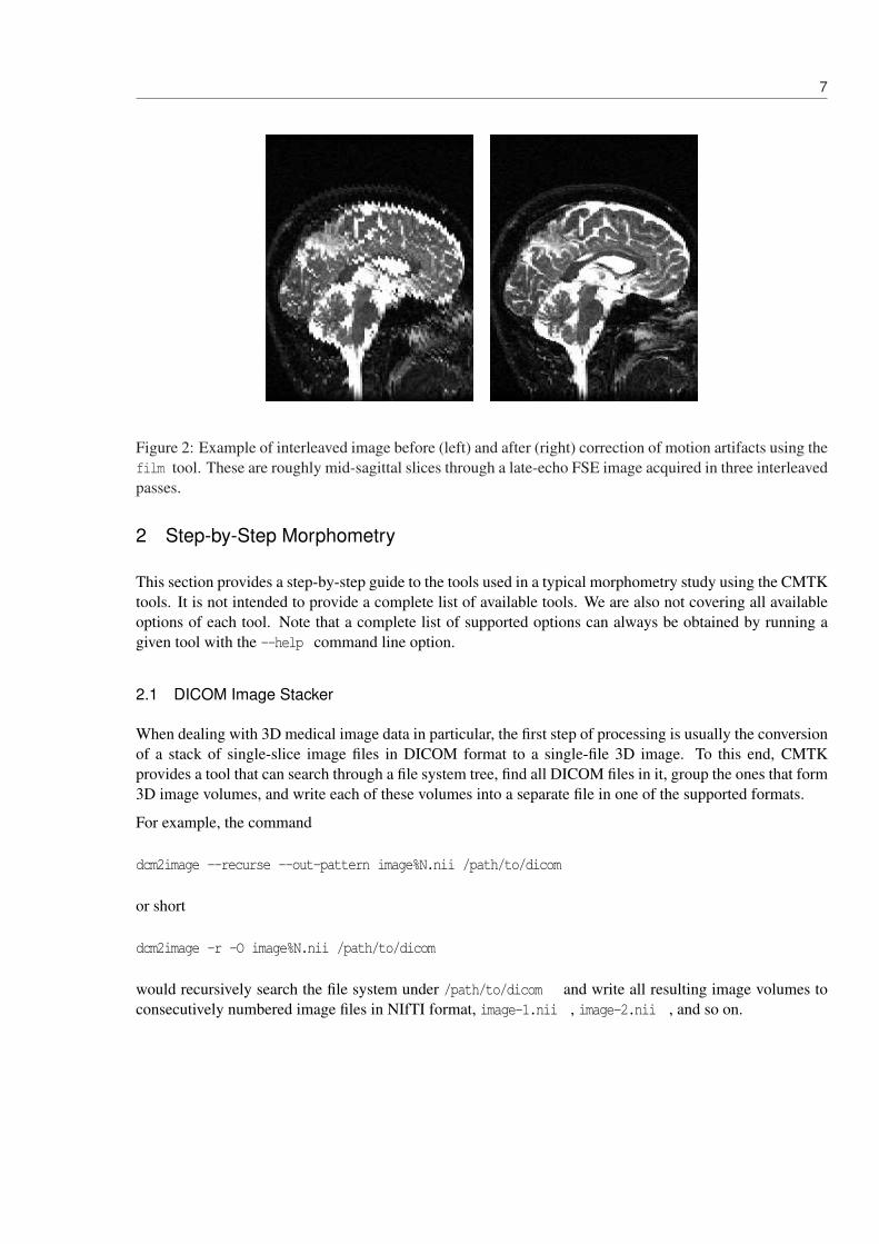
Figure 2: Example of interleaved image before (left) and after (right) correction of motion artifacts using thefilm tool. These are roughly mid-sagittal slices through a late-echo FSE image acquired in three interleavedpasses.

2 Step-by-Step Morphometry

This section provides a step-by-step guide to the tools used in a typical morphometry study using the CMTKtools. It is not intended to provide a complete list of available tools. We are also not covering all availableoptions of each tool. Note that a complete list of supported options can always be obtained by running agiven tool with the --help command line option.

2.1 DICOM Image Stacker

When dealing with 3D medical image data in particular, the first step of processing is usually the conversionof a stack of single-slice image files in DICOM format to a single-file 3D image. To this end, CMTKprovides a tool that can search through a file system tree, find all DICOM files in it, group the ones that form3D image volumes, and write each of these volumes into a separate file in one of the supported formats.

For example, the command

dcm2image --recurse --out-pattern image%N.nii /path/to/dicom

or short

dcm2image -r -O image%N.nii /path/to/dicom

would recursively search the file system under /path/to/dicom and write all resulting image volumes toconsecutively numbered image files in NIfTI format, image-1.nii , image-2.nii , and so on.

2.2 Interleaved Image Motion Artifact Correction 8

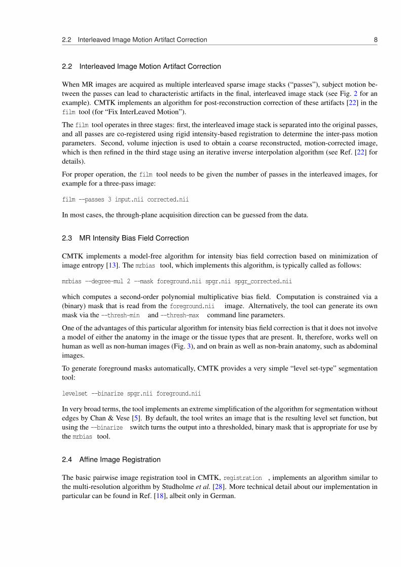
2.2 Interleaved Image Motion Artifact Correction

When MR images are acquired as multiple interleaved sparse image stacks (“passes”), subject motion be-tween the passes can lead to characteristic artifacts in the final, interleaved image stack (see Fig. 2 for anexample). CMTK implements an algorithm for post-reconstruction correction of these artifacts [22] in thefilm tool (for “Fix InterLeaved Motion”).

The film tool operates in three stages: first, the interleaved image stack is separated into the original passes,and all passes are co-registered using rigid intensity-based registration to determine the inter-pass motionparameters. Second, volume injection is used to obtain a coarse reconstructed, motion-corrected image,which is then refined in the third stage using an iterative inverse interpolation algorithm (see Ref. [22] fordetails).

For proper operation, the film tool needs to be given the number of passes in the interleaved images, forexample for a three-pass image:

film --passes 3 input.nii corrected.nii

In most cases, the through-plane acquisition direction can be guessed from the data.

2.3 MR Intensity Bias Field Correction

CMTK implements a model-free algorithm for intensity bias field correction based on minimization ofimage entropy [13]. The mrbias tool, which implements this algorithm, is typically called as follows:

mrbias --degree-mul 2 --mask foreground.nii spgr.nii spgr_corrected.nii

which computes a second-order polynomial multiplicative bias field. Computation is constrained via a(binary) mask that is read from the foreground.nii image. Alternatively, the tool can generate its ownmask via the --thresh-min and --thresh-max command line parameters.

One of the advantages of this particular algorithm for intensity bias field correction is that it does not involvea model of either the anatomy in the image or the tissue types that are present. It, therefore, works well onhuman as well as non-human images (Fig. 3), and on brain as well as non-brain anatomy, such as abdominalimages.

To generate foreground masks automatically, CMTK provides a very simple “level set-type” segmentationtool:

levelset --binarize spgr.nii foreground.nii

In very broad terms, the tool implements an extreme simplification of the algorithm for segmentation withoutedges by Chan & Vese [5]. By default, the tool writes an image that is the resulting level set function, butusing the --binarize switch turns the output into a thresholded, binary mask that is appropriate for use bythe mrbias tool.

2.4 Affine Image Registration

The basic pairwise image registration tool in CMTK, registration , implements an algorithm similar tothe multi-resolution algorithm by Studholme et al. [28]. More technical detail about our implementation inparticular can be found in Ref. [18], albeit only in German.

2.4 Affine Image Registration 9

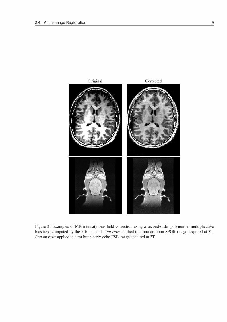
Original Corrected

Figure 3: Examples of MR intensity bias field correction using a second-order polynomial multiplicativebias field computed by the mrbias tool. Top row: applied to a human brain SPGR image acquired at 3T.Bottom row: applied to a rat brain early-echo FSE image acquired at 3T.

2.4 Affine Image Registration 10

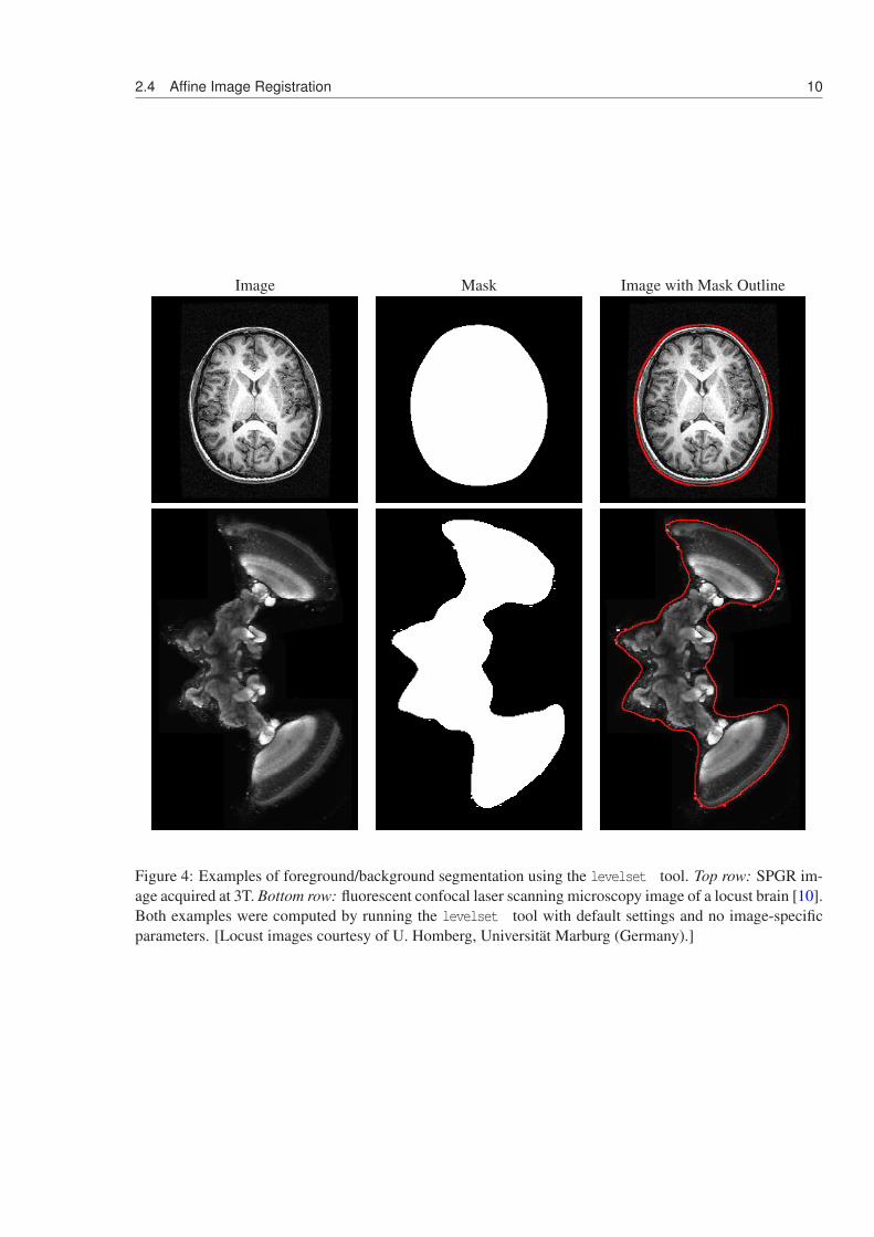
Image Mask Image with Mask Outline

Figure 4: Examples of foreground/background segmentation using the levelset tool. Top row: SPGR im-age acquired at 3T. Bottom row: fluorescent confocal laser scanning microscopy image of a locust brain [10].Both examples were computed by running the levelset tool with default settings and no image-specificparameters. [Locust images courtesy of U. Homberg, Universitat Marburg (Germany).]

2.5 Nonrigid Image Registration 11

In order to compute an affine registration between two images, the registration tool can be run as follows:

registration --initxlate --dofs 6,9 --auto-multi-levels 4 \-o affine.xform ref.nii flt.nii

This performs a registration of the floating image, flt.nii , to the reference image, ref.nii , where alloptimization and image resampling parameters are automatically determined for a 4-level multi-resolutionprocedure.

At each resolution level, the registration first optimizes 6 degrees of freedom (DOF), i.e., translation androtation of a 3D rigid transformation. Afterwards, 9 DOFs are optimized, i.e., three anisotropic scale factorsin addition to the translational and rotational parameters. Supported DOF numbers are: 0 (no registration,for testing), 3 (translation only), 6 (rigid: translation, rotation), 7 (similarity: translation, rotation, globalscale), 9 (translation, rotation, anisotropic scale), and 12 (full affine: translation, rotation, scale, and shears).

By default, registration uses the normalized mutual information [29] image similarity measure. Other avail-able similarity measures are: standard mutual information [14, 31] (--mi ), mean squared difference (--msd ),normalized cross-correlation (--ncc ), and correlation ratio [17] (--cr )

In the above example, the registration transformation is initialized (via --initxlate ) by translat-ing the floating image’s center to that of the reference image. For more complex initializations, themake_initial_affine tool can be used, which supports centers of mass, principal axes [1], and imageorientation vectors (e.g., as provided by the original DICOM data).

For example, in order to first initialize a transformation using principal axes and then use the result as theinitial transformation for intensity-based refinement, one would use the following sequence of commands:

make_initial_xform --principal-axes ref.nii flt.nii initial.xformregistration --initial initial.xform --dofs 6,9 --auto-multi-level 4 \

-o affine.xform ref.nii flt.nii

2.5 Nonrigid Image Registration

Pairwise nonrigid image registration in CMTK implements an algorithm introduced by Rueckert et al. [25],which uses as its transformation model multi-resolution free-form deformations based on cubic spline in-terpolation between sparse, uniformly distributed control points. Our particular implementation, which usesSMP parallelism to take advantage of multi-CPU systems, was described in Ref. [21].

A very simple nonrigid registration using a 40 mm control point grid, registering floating image flt.nii toreference image ref.nii based on an affine transformation affine.xform can be run as follows:

warp -o ffd40.xform --grid-spacing 40 --initial affine.xform ref.nii flt.nii

Typically, however, one would want to run a more sophisticated multi-level deformation, say with three re-finements (each reducing the grid spacing by 1/2 for a final spacing of 5 mm), and constrain the deformationusing grid bending energy:

warp -o ffd5.xform --grid-spacing 40 --refine 3 --energy-weight 1e-1 \--initial affine.xform ref.nii flt.nii

2.6 Reformating Registered Images 12

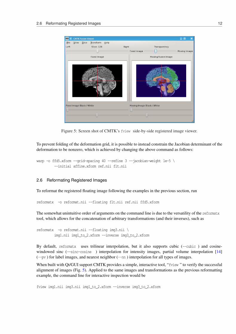
Figure 5: Screen shot of CMTK’s fview side-by-side registered image viewer.

To prevent folding of the deformation grid, it is possible to instead constrain the Jacobian determinant of thedeformation to be nonzero, which is achieved by changing the above command as follows:

warp -o ffd5.xform --grid-spacing 40 --refine 3 --jacobian-weight 1e-5 \--initial affine.xform ref.nii flt.nii

2.6 Reformating Registered Images

To reformat the registered floating image following the examples in the previous section, run

reformatx -o reformat.nii --floating flt.nii ref.nii ffd5.xform

The somewhat unintuitive order of arguments on the command line is due to the versatility of the reformatxtool, which allows for the concatenation of arbitrary transformations (and their inverses), such as

reformatx -o reformat.nii --floating img3.nii \img1.nii img1_to_2.xform --inverse img3_to_2.xform

By default, reformatx uses trilinear interpolation, but it also supports cubic (--cubic ) and cosine-windowed sinc (--sinc-cosine ) interpolation for intensity images, partial volume interpolation [14](--pv ) for label images, and nearest neighbor (--nn ) interpolation for all types of images.

When built with Qt/GUI support CMTK provides a simple, interactive tool, “fview ” to verify the successfulalignment of images (Fig. 5). Applied to the same images and transformations as the previous reformattingexample, the command line for interactive inspection would be

fview img1.nii img3.nii img1_to_2.xform --inverse img3_to_2.xform

2.7 Jacobian Determinant Maps 13

In general, fview is called with at least two parameters, the fixed and the moving image. These are followedby a sequence of transformations, each of which can be inverted by preceding it with “--inverse ”. Theeffective transformation applied to the moving image is the concatenation of the entire sequence.

The fview tool has a simple, intuitive user interface, which presents a side-by-side display of fixed andreformatted moving image, with variable transparent overlay of the fixed onto the moving image. Sliceorientation (axial, sagittal, coronal) and slice location can be adjusted, as can be interpolation kernel (lin-ear, cubic, sinc, nearest neighbour, partial volumes) and image color maps and window/level settings. Inaddition, the tool can selectively disable the nonrigid components of applied transformations and only applytheir global affine parts.

2.7 Jacobian Determinant Maps

Jacobian determinant maps, which are a staple ingredient of deformation-based morphometry studies [2],can also be computed using the reformatx tool. In the simplest case, we may want to compute the Ja-cobian determinant map for a transformation time1_to_time2.xform between two images, say imagestime1.nii and time1.nii acquired from the same subject at two time points. The command to computethe appropriate Jacobian determinant map, jacobian.nii , is then

reformatx -o jacobian.nii time1.nii --jacobian time1_to_time2.xform

More interestingly, say we want to compare these Jacobian maps from multiple subjects, all in the space ofa common atlas coordinate system. Then, instead of computing each map first in each subject’s coordinatesystem and then reformatting these maps into atlas space, we can directly compute the maps in atlas spaceby concatenation of transformations:

reformatx -o jacobian.nii atlas.nii \atlas_to_time1.xform --jacobian time1_to_time2.xform

Here, every sample coordinate in atlas space is first mapped to subject time 1 space viaatlas_to_time1.xform . For the resulting location, the Jacobian determinant of the longitudinal trans-formation, time1_to_time2.xform , is then computed.

Because the nonrigid transformations computed by the warp tool are generated via continuously differen-tiable B-spline basis functions, we can compute the Jacobian analytically at any location in the domain ofthe transformation, which means that the direct computation of Jacobians into atlas space does indeed avoidone interpolation of the Jacobian determinant map.

Note that the reformatx tool allows an arbitrary number of transformations to be listed both before and afterthe --jacobian switch, and any transformation can additionally be inverted by prefixing it with --inverse(affine transformations are inverted explicitly, whereas nonrigid transformations are inverted numerically).

2.8 Statistical Testing

For group comparisons of, for example, Jacobian determinant maps between different subject groups, thettest tool computes different types of t-tests (all two-tailed) and statistics. In the simplest case, two popu-lations A and B of maps can be tested against one another as follows:

2.9 Atlas-based Segmentation 14

ttest -o pvalues.nii --tstats-file tstats.nii \jacobianA1.nii jacobianA2.nii -- jacobianB1.nii jacobianB2.nii

This computes a pixel-wise two-tailed unpaired t-test between the two lists of images separated with “-- ”on the command line. The resulting p-values image is then written to pvalues.nii , and the t-statistics arealso written to tstats.nii .

To compute a two-tailed paired t-test, make sure that there are an equal number of images before andafter the “-- ” separator and that corresponding images in both groups are in the same order, then add the--paired option and run

ttest -o pvalues.nii --tstats-file tstats.nii --paired \jacobianA1.nii jacobianA2.nii -- jacobianB1.nii jacobianB2.nii

Invoking ttest with only a single group of images (without “-- ” anywhere in the image list), will computea single-sample t-test, that is, a test for significant differences from zero:

ttest -o pvalues.nii --tstats-file tstats.nii jacobianA1.nii jacobianA2.nii

2.9 Atlas-based Segmentation

Atlas-based segmentation uses correspondence between a previously segmented image (the atlas) and anew, unsegmented image to create a segmentation of the latter [16]. This relatively simple idea can easilybe implemented using CMTK’s registration , warp , and reformatx tools. For convenience, however,CMTK also provides an integrated atlas-based segmentation tool, which can be run as follows:

asegment input_image.nii atlas_image.nii atlas_labels.nii output_labels.nii

Here, it is assumed that input_image.nii is a new, unsegmented image, for example an MR scan of a newsubject, atlas_image.nii is the intensity image of the atlas, and atlas_labels.nii is the label image ofthe atlas, i.e., the segmentation corresponding to the atlas intensity image. The tool will then register the atlasto the new image, reformat that atlas label map onto it, and write the result to the file output_labels.nii .

The standard atlas of CMTK is the SRI24 atlas [23, 24], which comprises several different channels ofMR image information, as well as scalar diffusion measures, tissue probability maps, and segmentationmaps. If CMTK is configured and built with SRI24 support (by setting the CMTK_ROOT_PATH_SRI24 CMakevariable), then a simplified segmentation tool, asegment_sri24 , which uses the SRI24 atlas is also built.

This tool, by default, registers a given image to the SPGR channel of the SRI24 atlas. It then createsand writes a segmentation map based on the “tzo116plus” label map, which derived from the “automaticanatomic labelling” (AAL) parcellation map by Tzourio-Mazoyer et al. [30]. This is achieved simply byrunning

asegment_sri24 input_image.nii output_segmentation.nii

Different atlas channels can be used for registration, selected using the --registration-channel com-mand line option: “spgr ” for T1-weighted SPGR, which is the default,“early-fse ” for early-echo (protondensity-weighted) FSE , “late-fse ” for late-echo (T2-weighted) FSE, and “fa ” for DTI-derived fractionalanisotropy.

2.9 Atlas-based Segmentation 15

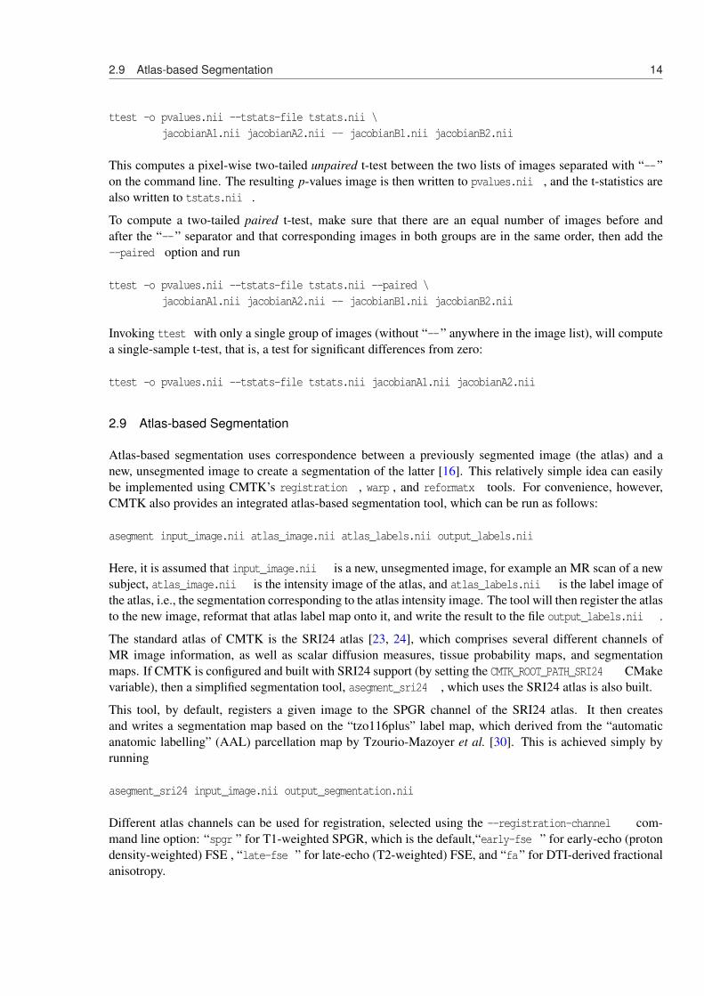
Figure 6: Integration of asegment sri24 tool into 3D Slicer, and result of segmentation using the“tzo116plus ” label map.

Likewise, different label maps are available for the output, selected by the --label-map command lineoption: “tzo116plus ” for the extended Tzourio-Mazoyer map, “lpba40 ” for a segmentation based on the40-subject LONI Probabilistic Brain Atlas [27] (LPBA40), and “tissue ” for a maximum-likelihood three-tissue (CSF, WM, GM) segmentation.

The integration of a complete atlas-based segmentation workflow with a pre-defined atlas is particularlyconvenient when using CMTK’s tools from within the 3D Slicer software. Fig. 6 shows an example ofthe Slicer-generated user interface for the asegment_sri24 tool, as well as the result of an atlas-basedsegmentation using the “tzo116plus ” label map.

16

3 Atlas Construction

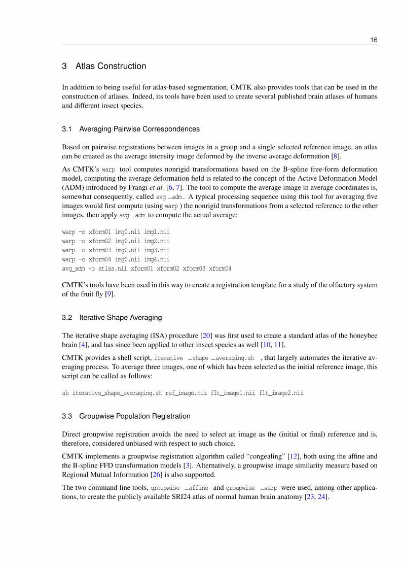
In addition to being useful for atlas-based segmentation, CMTK also provides tools that can be used in theconstruction of atlases. Indeed, its tools have been used to create several published brain atlases of humansand different insect species.

3.1 Averaging Pairwise Correspondences

Based on pairwise registrations between images in a group and a single selected reference image, an atlascan be created as the average intensity image deformed by the inverse average deformation [8].

As CMTK’s warp tool computes nonrigid transformations based on the B-spline free-form deformationmodel, computing the average deformation field is related to the concept of the Active Deformation Model(ADM) introduced by Frangi et al. [6, 7]. The tool to compute the average image in average coordinates is,somewhat consequently, called avg adm . A typical processing sequence using this tool for averaging fiveimages would first compute (using warp ) the nonrigid transformations from a selected reference to the otherimages, then apply avg adm to compute the actual average:

warp -o xform01 img0.nii img1.niiwarp -o xform02 img0.nii img2.niiwarp -o xform03 img0.nii img3.niiwarp -o xform04 img0.nii img4.niiavg_adm -o atlas.nii xform01 xform02 xform03 xform04

CMTK’s tools have been used in this way to create a registration template for a study of the olfactory systemof the fruit fly [9].

3.2 Iterative Shape Averaging

The iterative shape averaging (ISA) procedure [20] was first used to create a standard atlas of the honeybeebrain [4], and has since been applied to other insect species as well [10, 11].

CMTK provides a shell script, iterative shape averaging.sh , that largely automates the iterative av-eraging process. To average three images, one of which has been selected as the initial reference image, thisscript can be called as follows:

sh iterative_shape_averaging.sh ref_image.nii flt_image1.nii flt_image2.nii

3.3 Groupwise Population Registration

Direct groupwise registration avoids the need to select an image as the (initial or final) reference and is,therefore, considered unbiased with respect to such choice.

CMTK implements a groupwise registration algorithm called “congealing” [12], both using the affine andthe B-spline FFD transformation models [3]. Alternatively, a groupwise image similarity measure based onRegional Mutual Information [26] is also supported.

The two command line tools, groupwise affine and groupwise warp were used, among other applica-tions, to create the publicly available SRI24 atlas of normal human brain anatomy [23, 24].

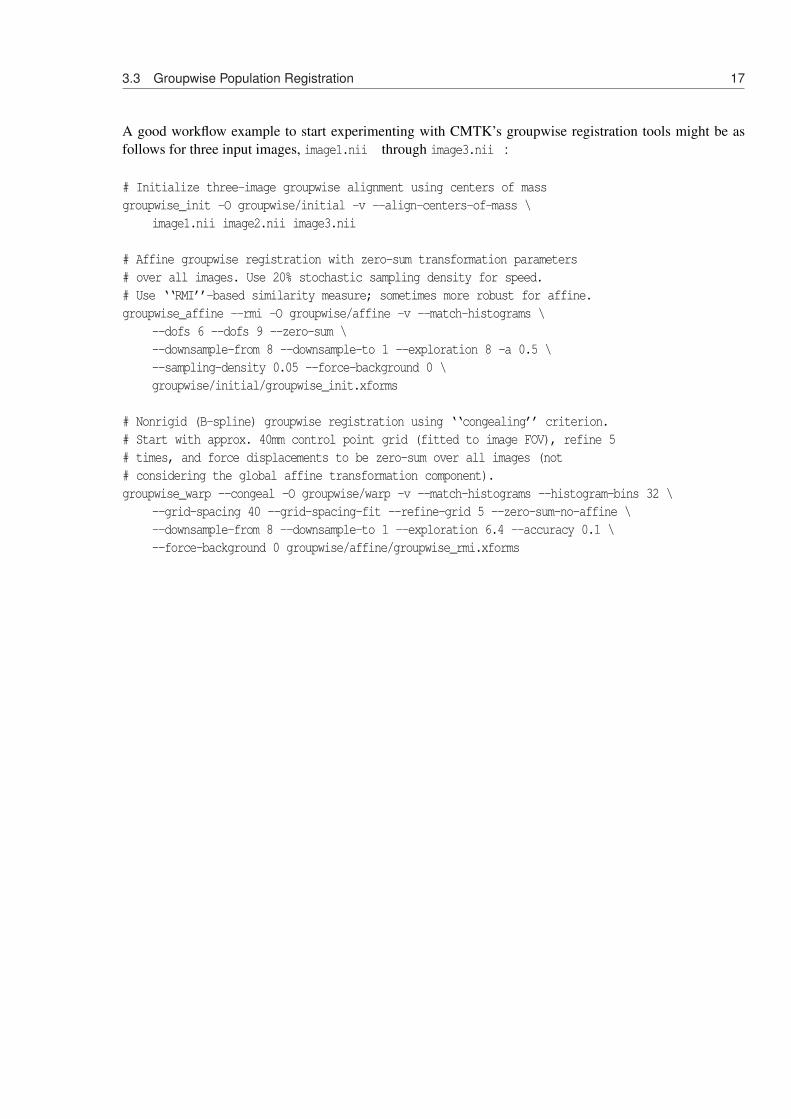
3.3 Groupwise Population Registration 17

A good workflow example to start experimenting with CMTK’s groupwise registration tools might be asfollows for three input images, image1.nii through image3.nii :

# Initialize three-image groupwise alignment using centers of massgroupwise_init -O groupwise/initial -v --align-centers-of-mass \

image1.nii image2.nii image3.nii

# Affine groupwise registration with zero-sum transformation parameters# over all images. Use 20% stochastic sampling density for speed.# Use ‘‘RMI’’-based similarity measure; sometimes more robust for affine.groupwise_affine --rmi -O groupwise/affine -v --match-histograms \

--dofs 6 --dofs 9 --zero-sum \--downsample-from 8 --downsample-to 1 --exploration 8 -a 0.5 \--sampling-density 0.05 --force-background 0 \groupwise/initial/groupwise_init.xforms

# Nonrigid (B-spline) groupwise registration using ‘‘congealing’’ criterion.# Start with approx. 40mm control point grid (fitted to image FOV), refine 5# times, and force displacements to be zero-sum over all images (not# considering the global affine transformation component).groupwise_warp --congeal -O groupwise/warp -v --match-histograms --histogram-bins 32 \

--grid-spacing 40 --grid-spacing-fit --refine-grid 5 --zero-sum-no-affine \--downsample-from 8 --downsample-to 1 --exploration 6.4 --accuracy 0.1 \--force-background 0 groupwise/affine/groupwise_rmi.xforms

18

4 More Gory Details

4.1 Registration Options for Image Pre-Processing

Both the affine and nonrigid pairwise image registration, registration and warp , support a number of pre-processing operations that can be applied to the reference and floating image on-the-fly, prior to registration.The most commonly used of these are:

• Data Class: For each image, the “class” of the image data can be defined. This can be “grey,” “binary,”or “label.” Typically, both images should have data in the same class. When the data class is set to“label,” the registration algorithm uses nearest neighbour instead of trilinear interpolation, and thenumbers of histogram bin are set to the number of labels in each image rather than being adjustedbased on the intensity range and number of pixels.

• Thresholding: Upper and lower thresholds can be defined to truncate the image intensities.

• Cropping: Images can be cropped, based on either image index ranges or image coordinate ranges.The registration tool implements a volume clipping algorithm [19] that considerably speeds upregistration of cropped images. Cropping can also improve registration accuracy and robustness byexcluding non-informative areas of the images.

• Histogram Pruning: For a given number of histogram bins (128 is typically a good value), this op-eration truncates the intensity range of the image such that both the lowest and the highest histogrambin receive 1/NumberOfBins of the total number of image samples. This is quite effective to preventdegeneration of histograms by extreme image intensities due to noise.

Histogram Matching: Using the --match-histograms option, the intensities of the floating image can berescaled to match the distribution of the reference image. This is a common pre-processing operator toallow, for example, registration of inter-subject images using the mean squared differences metric.

Setting value outside FOV: A default value for data outside the floating image FOV can be defined usingthe --force-outside-value option. This artificially increases the overlapping image region that can beconsidered for registration, which may help increase registration robustness.

4.2 GPU-Accelerated Tools

Starting with the 1.4 release series, CMTK is adding support for accelerating computations using general-purpose graphics processing units (GPGPU). As of release 1.4.2, GPU support is available for level setsegmentation, , MR bias field correction, and image symmetry plane computation.

For the time being, GPU support is limited to the nVidia CUDA programming model, but OpenCL may besupported in future releases. The command line tools that provide CUDA support are distinguished fromtheir CPU-only counterparts by the suffix “ cuda ” such that the GPU-analog for the mrbias tool would bemrbias cuda . We chose to separate CPU and GPU tools so that both could be built jointly on a system withGPU hardware and drivers, but the CPU tools could still be used on a system without these capabilities.

Note that while every effort is made to keep the command line syntax and semantics identical for CPU andGPU tools, this is not always fully possible.

References 19

Acknowledgments

Much of the effort required to get CMTK ready for release as open source software was performed byMike Hasak at SRI. Calvin R. Maurer, Jr., wrote the original implementation of his linear-time algorithmfor the Euclidean distance transform [15], which cmtk::UniformDistanceMap is based on, and kindlyagreed to distribution of this derived code under the GPL. Likewise, Daniel Russakoff kindly agreed to GPLlicensing of code he wrote for entropy computation based on covariance matrices, as he used it in his workon Regional Mutual Information [26]. Greg Jefferis provided numerous bug reports and fixes, includingmuch of the details required to get CMTK compiled and working on the MacOS platform.

References

[1] N. M. Alpert, J. F. Bradshaw, D. Kennedy, and J. A. Correia. “The principal axes transformation – amethod for image registration.” Journal of Nuclear Medicine, 31(10):1717–1722, 1990. 2.4

[2] J. Ashburner, C. Hutton, R. Frackowiak, I. Johnsrude, C. Price, and K. Friston. “Identifying globalanatomical differences: Deformation-based morphometry.” Human Brain Mapping, 6(5–6):348–357,1998. http://dx.doi.org/10.1002/(SICI)1097-0193(1998)6:5/6<348::AID-HBM4>3.0.CO;2-P . 2.7

[3] S. K. Balci, P. Golland, M. Shenton, and W. M. Wells. “Free-form B-spline deformation model forgroupwise registration.” In “MICCAI 2007 Workshop Statistical Registration: Pair-wise and Group-wise Alignment and Atlas Formation,” pp. 23–30. 2007. 3.3

[4] R. Brandt, T. Rohlfing, J. Rybak, S. Krofczik, A. Maye, M. Westerhoff, H.-C. Hege, and R. Men-zel. “Three-dimensional average-shape atlas of the honeybee brain and its applications.” Journalof Comparative Neurology, 492(1):1–19, 2005. http://dx.doi.org/10.1002/cne.20644 . PMID16175557. 3.2

[5] T. F. Chan and L. A. Vese. “Active contours without edges.” IEEE Transactions on Image Processing,10(2):266–277, 2001. http://dx.doi.org/S1057-7149(01)00819-3 . 2.3

[6] A. F. Frangi, D. Rueckert, J. A. Schnabel, and W. J. Niessen. “Automatic 3D ASM construction viaatlas-based landmarking and volumetric elastic registration.” In M. F. Insana and R. M. Leahy (eds.),“Information Processing in Medical Imaging: 17th International Conference, IPMI 2001, Davis, CA,USA, June 18-22, 2001, Proceedings,” vol. 2082 of Lecture Notes in Computer Science, pp. 78–91.Springer-Verlag, Berlin/Heidelberg, 2001. 3.1

[7] A. F. Frangi, D. Rueckert, J. A. Schnabel, and W. J. Niessen. “Automatic construction of multiple-object three-dimensional statistical shape models: application to cardiac modeling.” IEEE Transac-tions on Medical Imaging, 21(9):1151–1166, 2002. 3.1

[8] A. Guimond, J. Meunier, and J.-P. Thirion. “Average brain models: A convergence study.” ComputerVision and Image Understanding, 77(2):192–210, 2000. http://dx.doi.org/10.1006/cviu.1999.0815 . 3.1

[9] G. S. Jefferis, C. J. Potter, A. M. Chan, E. C. Marin, T. Rohlfing, C. R. Maurer, Jr., and L. Luo. “Com-prehensive maps of Drosophila higher olfactory centers: Spatially segregated fruit and pheromonerepresentation.” Cell, 128(6):1187–1203, 2007. PMID 17382886, PMC 1885945. 3.1

References 20

[10] A. E. Kurylas, T. Rohlfing, S. Krofczik, A. Jenett, and U. Homberg. “Standardized atlas of the brainof the desert locust, schistocerca gregaria.” Cell and Tissue Research, 333(1):125–145, 2008. http://dx.doi.org/10.1007/s00441-008-0620-x . PMID 18504618. 4, 3.2

[11] P. Kvello, B. B. Løfaldli, J. Rybak, R. Menzel, and H. Mustaparta. “Digital, three-dimensional averageshaped atlas of the heliothis virescens brain with integrated gustatory and olfactory neurons.” Frontiersin Systems Neuroscience, 3, 2009. http://dx.doi.org/10.3389/neuro.06/014.2009 . 3.2

[12] E. G. Learned-Miller. “Data driven image models through continuous joint alignment.” IEEE Trans-actions on Pattern Analysis and Machine Intelligence, 28(2):236–250, 2006. http://dx.doi.org/10.1109/TPAMI.2006.34 . 3.3

[13] B. Likar, M. A. Viergever, and F. Pernus. “Retrospective correction of MR intensity inhomogeneityby information minimization.” IEEE Transactions on Medical Imaging, 20(12):1398–1410, 2001.http://dx.doi.org/10.1109/42.974934 . 2.3

[14] F. Maes, A. Collignon, D. Vandermeulen, G. Marchal, and P. Suetens. “Multimodality image registra-tion by maximisation of mutual information.” IEEE Transactions on Medical Imaging, 16(2):187–198,1997. 2.4, 2.6

[15] C. R. Maurer, Jr., R. Qi, and V. Raghavan. “A linear time algorithm for computing exact Euclideandistance transforms of binary images in arbitrary dimensions.” IEEE Transactions on Pattern Analysisand Machine Intelligence, 25(2):265–270, 2003. 4.2

[16] M. I. Miller, G. E. Christensen, Y. Amit, and U. Grenander. “Mathematical textbook of deformableneuroanatomies.” Proceedings of the National Academy of Sciences of the U.S.A., 90(24):11944–11948, 1993. 2.9

[17] A. Roche, G. Malandain, X. Pennec, and N. Ayache. “The correlation ratio as a new similarity measurefor multimodal image registration.” In W. M. Wells, III., A. C. F. Colchester, and S. Delp (eds.),“Medical Image Computing and Computer-Assisted Intervention - MICCAI’98, First InternationalConference, Cambridge, MA, USA, October 11-13, 1998, Proceedings,” vol. 1496 of Lecture Notes inComputer Science, pp. 1115–1124. Springer-Verlag, 1998. 2.4

[18] T. Rohlfing. Multimodale Datenfusion fur die bildgesteuerte Neurochirurgie und Strahlentherapie.Ph.D. thesis, Technische Universitat Berlin, 2000. 2.4

[19] T. Rohlfing. “Incremental method for computing the intersection of discretely sampled m-dimensionalimages with n-dimensional boundaries.” In M. Sonka and J. M. Fitzpatrick (eds.), “Medical Imaging:Image Processing,” vol. 5032 of Proceedings of SPIE, pp. 1346–1354. 2003. http://dx.doi.org/10.1117/12.483556 . 4.1

[20] T. Rohlfing, R. Brandt, C. R. Maurer, Jr., and R. Menzel. “Bee brains, B-splines and computationaldemocracy: Generating an average shape atlas.” In L. Staib (ed.), “IEEE Workshop on MathematicalMethods in Biomedical Image Analysis,” pp. 187–194. IEEE Computer Society, Los Alamitos, CA,Kauai, HI, 2001. ISBN 0-7695-1336-0. http://dx.doi.org/10.1109/MMBIA.2001.991733 . 3.2

[21] T. Rohlfing and C. R. Maurer, Jr. “Nonrigid image registration in shared-memory multiprocessor envi-ronments with application to brains, breasts, and bees.” IEEE Transactions on Information Technologyin Biomedicine, 7(1):16–25, 2003. PMID 12670015. 2.5

References 21

[22] T. Rohlfing, M. H. Rademacher, and A. Pfefferbaum. “Volume reconstruction using inverse interpola-tion: application to interleaved image motion correction.” In D. Metaxas, L. Axel, G. Fichtinger, andG. Szekely (eds.), “Medical Image Computing and Computer-Assisted Intervention — MICCAI 2008.11th International Conference, New York, NY, USA, September 6-10, 2008, Proceedings, Part I,” vol.5241 of Lecture Notes in Computer Science, pp. 798–806. Springer-Verlag, Berlin/Heidelberg, 2008.http://dx.doi.org/10.1007/978-3-540-85988-8_95 . PMID 18979819, PMC 2646840. 2.2

[23] T. Rohlfing, N. M. Zahr, E. V. Sullivan, and A. Pfefferbaum. “The SRI24 multi-channel brain atlas:Construction and applications.” In J. M. Reinhardt and J. P. W. Pluim (eds.), “Medical Imaging 2008:Image Processing,” vol. 6914 of Proceedings of SPIE, p. 691409. Bellingham, WA, 2008. http://dx.doi.org/10.1117/12.770441 . PMID 19183706, PMC 2633114. 2.9, 3.3

[24] T. Rohlfing, N. M. Zahr, E. V. Sullivan, and A. Pfefferbaum. “The SRI24 multichannel atlas of normaladult human brain structure.” Human Brain Mapping, 31(5):798–819, 2010. http://dx.doi.org/10.1002/hbm.20906 . PMID 20017133. 2.9, 3.3

[25] D. Rueckert, L. I. Sonoda, C. Hayes, D. L. G. Hill, M. O. Leach, and D. J. Hawkes. “Nonrigidregistration using free-form deformations: Application to breast MR images.” IEEE Transactions onMedical Imaging, 18(8):712–721, 1999. 2.5

[26] D. B. Russakoff, C. Tomasi, T. Rohlfing, and C. R. Maurer, Jr. “Image similarity using mutual in-formation of regions.” In “Computer Vision - ECCV 2004: 8th European Conference on ComputerVision, Prague, Czech Republic, May 11-14, 2004. Proceedings, Part III,” vol. 3023 of Lecture Notesin Computer Science, pp. 596–607. Springer-Verlag, Berlin/Heidelberg, 2004. 3.3, 4.2

[27] D. W. Shattuck, M. Mirza, V. Adisetiyo, C. Hojatkashani, G. Salamon, K. L. Narr, R. A. Poldrack,R. M. Bilder, and A. W. Toga. “Construction of a 3D probabilistic atlas of human cortical struc-tures.” NeuroImage, 39(3):1064–1080, 2008. http://dx.doi.org/10.1016/j.neuroimage.2007.09.031 . 2.9

[28] C. Studholme, D. L. G. Hill, and D. J. Hawkes. “Automated three-dimensional registration of magneticresonance and positron emission tomography brain images by multiresolution optimization of voxelsimilarity measures.” Medical Physics, 24(1):25–35, 1997. 2.4

[29] C. Studholme, D. L. G. Hill, and D. J. Hawkes. “An overlap invariant entropy measure of 3D med-ical image alignment.” Pattern Recognition, 32(1):71–86, 1999. http://dx.doi.org/10.1016/S0031-3203(98)00091-0 . 2.4

[30] N. Tzourio-Mazoyer, B. Landeau, D. Papathanassiou, F. Crivello, O. Etard, N. Delcroix, B. Mazoyer,and M. Joliot. “Automated anatomical labeling of activations in SPM using a macroscopic anatomicalparcellation of the MNI MRI single-subject brain.” NeuroImage, 15(1):273–289, 2002. http://dx.doi.org/10.1006/nimg.2001.0978 . 2.9

[31] W. M. Wells, P. A. Viola, H. Atsumi, S. Nakajima, and R. Kikinis. “Multi-modal volume registrationby maximization of mutual information.” Medical Image Analysis, 1(1):35–51, 1996. http://dx.doi.org/10.1016/S1361-8415(01)80004-9 . 2.4

Index

3D Slicer software, 6, 15

Artifactsintensity bias field, 8motion, 8

AtlasAAL template, 14construction, 16LPBA40, 15SRI24, 14, 16

CMTKlicensing, 3

CMTK Toolsasegment , 14avg adm , 16dcm2image , 7film , 8groupwise warp , 16groupwise affine , 16make initial affine , 11mrbias , 8reformatx , 12registration , 8, 18ttest , 13warp , 11, 16, 18

Coordinate system, 3

degrees of freedom, 11DICOM, 7

GPU, 18CUDA, 18OpenCL, 18

GUIaligned image pair viewer, 12triplanar image viewer, 3

Imagefixed, 5floating, 5interleaved MR, 8moving, 5reference, 5

Jacobiandeterminant maps, 13

registration constraint, 12

Registrationaffine, 11groupwise, 16nonrigid, 11pairwise, 5, 8principal axes, 11terminology, 5

Segmentationatlas-based, 14level set, 8, 18